“Cramming” Before the Exam:

Estimating the Causal Effect of Exam Preparatory

Programs in a Non-randomized Study

Ming-sen Wang

Department of Economics

University of Arizona∗†

May 04, 2012

FIRST DRAFT: January 12, 2012

Abstract

In this empirical paper, I estimate the impact of attending exam preparatory pro-

grams, in particular “cram schools,” on students’ academic performance. I measure

the outcome by admission to a public high school and an “elite” high school. Fo-

cusing on the problem that students are not randomly assigned to “cram schools,”

I approach the issue using propensity score matching and a Bayesian simultaneous-

equations model. Using data from a survey of Taiwanese junior high school students

in the Taiwan Youth Project, I find evidence that there is an insignificantly negative

∗I am indebted for continuous guidance of Ronald Oaxaca and helpful comments and suggestions

from Katherine Barnes, Price Fishback, Keisuke Hirano, and Tiemen Woutersen. I have benefited from

discussions with Mario Samano-Sanchez, Sandeep Shetty, and Ju-Chun Yen. All the remaining errors

are of my own. E-mail: mswang@email.arizona.edu; the latest version of the paper can be found at:

http://www.u.arizona.edu/∼mswang.†Data analyzed in this paper were collected by the research project Taiwan Youth Project sponsored

by the Academia Sinica ( AS-93-TP-C01). This research project was carried out by Institute of Sociology,

Academia Sinica, and directed by Chin-Chun Yi. The Center for Survey Research of Academia Sinica

is responsible for the data distribution. The authors appreciate the assistance in providing data by the

institutes and individuals aforementioned. The views expressed herein are the authors’ own.

1

sorting into exam preparatory programs and attending an exam preparatory program

improves a student’s possibility of being admitted to a public high school or an “elite”

high school. Both approaches indicate similar positive treatment effects.

1 Introduction

In many East Asian countries, such as Taiwan and Japan, attendance of the so-called “cram

school” is prevalent. A “cram school” is a type of shadow education that is aimed at

improving a student’s exam writing skills. Attending “cram school” imposes additional

burdens on a student and her family. It puts additional stress on a student since it requires

time and effort. It puts financial loads on parents because sending a child to a program for

a month can cost more than tuition fees for a semester in a public school.

Given the prevalence and important role of exam preparatory programs in the education

system, it is surprising that there are few rigorous evaluations. One problem is that students

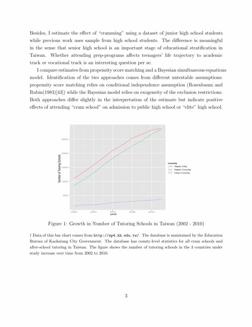
often self-select into these prep-programs.(Jackson(2012)[33]) As shown in Figure (1), the

number of “cram schools” in Taiwan grows steadily. However, there has never been a rigorous

proof that attending exam prep-program indeed improves students placement of high school.

In a seminal paper, Stevenson and Baker (1992)[47] point out possible factors that foster

“cram schools”: (1) the use of a centrally administered examination, (2) the use of “con-

test rules” instead of “sponsorship rules”, and (3) tight linkages between the outcomes of

educational allocation in elementary and secondary schooling and future educational oppor-

tunities. Taiwanese society has all these factors. Graduates of an “elite” university in Taiwan

have significant advantages in the labor market (Lin (1983) [36])1. A student’s performance

in the Joint High-school Entrance Exam and the Joint College Entrance Exam is strongly

linked to future opportunities. It causes a prevalence of “cram schools” in Taiwan and makes

Taiwan an ideal candidate to study.

The paper distinguishes itself from previous work in two ways (See Stevenson and Baker

(1992)[47] and Lin et al.(2006)[37]). Firstly,while other literatures define exam performances

as outcome, I focus on admission to public high school and “elite” high school as outcome of

interest to avoid selection issue related to taking the Joint Entrance Exam. Since Taiwan has

undergone a significant education reform lately as we will discuss in the next section, focusing

on admission circumvents complication of modeling and necessity of exclusion restrictions.

1Notice this result can hardly be interpreted as causal since the research does not control for the selectionthat the graduates of an“elite” university in Taiwan is productive to begin with.

2

Besides, I estimate the effect of “cramming” using a dataset of junior high school students

while previous work uses sample from high school students. The difference is meaningful

in the sense that senior high school is an important stage of educational stratification in

Taiwan. Whether attending prep-programs affects teenagers’ life trajectory to academic

track or vocational track is an interesting question per se.

I compare estimates from propensity score matching and a Bayesian simultaneous-equations

model. Identification of the two approaches comes from different untestable assumptions:

propensity score matching relies on conditional independence assumption (Rosenbaum and

Rubin(1983)[43]) while the Bayesian model relies on exogeneity of the exclusion restrictions.

Both approaches differ slightly in the interpretation of the estimate but indicate positive

effects of attending “cram school” on admission to public high school or “elite” high school.

year

Numb

er of

Tutor

ing S

choo

ls

500

1000

1500

2000

2500

2002 2004 2006 2008 2010

county

Taipei City

Taipei County

Yilan County

Figure 1: Growth in Number of Tutoring Schools in Taiwan (2002 - 2010)

† Data of this bar chart comes from http://ap4.kh.edu.tw/. The database is maintained by the Education

Bureau of Kaohsiung City Government. The database has county-level statistics for all cram schools and

after-school tutoring in Taiwan. The figure shows the number of tutoring schools in the 3 countries under

study increase over time from 2002 to 2010.

3

1.1 Institutional Backgrounds

In 1987, Taiwan ended the martial law that has been in effect since 1949. Along with the

freer and more opener political atmosphere, many civil groups started to request reforms

in the education system. One of the most significant changes was to replace the old Joint

Exam System with the new Multi-Opportunities System. In the old system, every junior

high graduate had to attend the Joint High-school Entrance Exam that took place in the

summer after the graduation. Students were ranked based on their exam grades. The ranking

determined their priorities to choose an academic high school or a vocational high school.

Their performance on the Joint High-school Entrance Exam determined their high school.

The Exam decided the educational stratification.

In 2001, the Ministry of Education officially executed the new Multi-Opportunities Sys-

tem. The main idea of the new system is to separate admissions from exams. Two joint

exams, the Basic Scholastic Ability Test and the Joint High-school Entrance Exam, are held

in a school year to provide students one more chance. Under the new system, students

can be admitted to high schools through multiple channels, such as (1) the Joint Entrance

Exam, (2) the Special Admission Quotas for Recommended Students, and (3) Other Chan-

nels without Entrance Exam Grades. Even though using grades of the Joint Entrance Exam

as outcome provides a universal measurement, it involves complication to handle selection

to take the Exam. Defining admission as outcome very much simplifies the modeling.

1.2 Literature Review

Human capital investment has been a research focus ever since Becker(1962)[7]’s first rigorous

treatment on the topic. A large literature is dedicated to estimating the returns of the

formal schooling.(See Ashenfelter and Krueger (1994)[6]; Card (1995)[11]; Card(2001)[12];

Belzil(2007)[10]) Regan et al.(2007)[41], on the other hand, focuses on the optimal level of

stopping schooling instead of estimating the rate of returns.

On the other hand, if a prep-program does not directly increase human capital and it

only affects a student’s exam performance, the program can be considered as a way to reduce

high school costs. It is of particular interest to investigate whether “cram school” increases

the likelihood of being admitted to public high school. Admission to an “elite” high school

increases the likelihood of being admitted to a better public university2. Again, tuition fees

2Since Taiwanese government subsidizes higher education heavily, public universities in general are rankedas better universities.

4

in a public university are significantly lower than in a private university. Lower tuition fees

affect a student’s decision of stopping schooling.

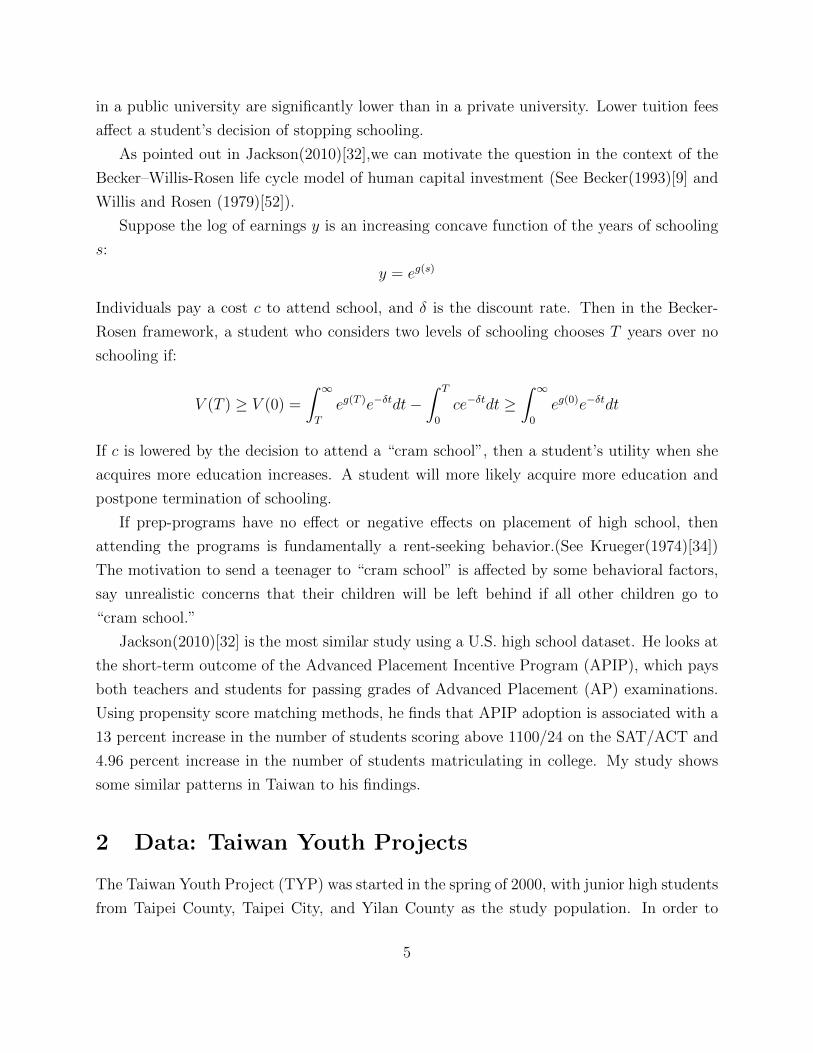
As pointed out in Jackson(2010)[32],we can motivate the question in the context of the

Becker–Willis-Rosen life cycle model of human capital investment (See Becker(1993)[9] and

Willis and Rosen (1979)[52]).

Suppose the log of earnings y is an increasing concave function of the years of schooling

s:

y = eg(s)

Individuals pay a cost c to attend school, and δ is the discount rate. Then in the Becker-

Rosen framework, a student who considers two levels of schooling chooses T years over no

schooling if:

V (T ) ≥ V (0) =

∫ ∞T

eg(T )e−δtdt−∫ T

0

ce−δtdt ≥∫ ∞0

eg(0)e−δtdt

If c is lowered by the decision to attend a “cram school”, then a student’s utility when she

acquires more education increases. A student will more likely acquire more education and

postpone termination of schooling.

If prep-programs have no effect or negative effects on placement of high school, then

attending the programs is fundamentally a rent-seeking behavior.(See Krueger(1974)[34])

The motivation to send a teenager to “cram school” is affected by some behavioral factors,

say unrealistic concerns that their children will be left behind if all other children go to

“cram school.”

Jackson(2010)[32] is the most similar study using a U.S. high school dataset. He looks at

the short-term outcome of the Advanced Placement Incentive Program (APIP), which pays

both teachers and students for passing grades of Advanced Placement (AP) examinations.

Using propensity score matching methods, he finds that APIP adoption is associated with a

13 percent increase in the number of students scoring above 1100/24 on the SAT/ACT and

4.96 percent increase in the number of students matriculating in college. My study shows

some similar patterns in Taiwan to his findings.

2 Data: Taiwan Youth Projects

The Taiwan Youth Project (TYP) was started in the spring of 2000, with junior high students

from Taipei County, Taipei City, and Yilan County as the study population. In order to

5

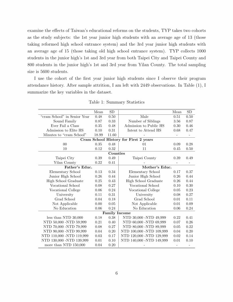
examine the effects of Taiwan’s educational reforms on the students, TYP takes two cohorts

as the study subjects: the 1st year junior high students with an average age of 13 (those

taking reformed high school entrance system) and the 3rd year junior high students with

an average age of 15 (those taking old high school entrance system). TYP collects 1000

students in the junior high’s 1st and 3rd year from both Taipei City and Taipei County and

800 students in the junior high’s 1st and 3rd year from Yilan County. The total sampling

size is 5600 students.

I use the cohort of the first year junior high students since I observe their program

attendance history. After sample attrition, I am left with 2449 observations. In Table (1), I

summarize the key variables in the dataset.

Table 1: Summary Statistics

Mean SD Mean SD“cram School” in Senior Year 0.48 0.50 Male 0.51 0.50

Sound Family 0.87 0.33 Number of Siblings 3.56 0.87Ever Fail a Class 0.35 0.48 Admission to Public HS 0.30 0.46

Admission to Elite HS 0.10 0.31 Intent to Attend HS 0.68 0.47Minutes to “cram School” 18.99 11.60 - - -

Cram School History for First 2 years00 0.35 0.48 01 0.09 0.2810 0.12 0.32 11 0.45 0.50

CountiesTaipei City 0.39 0.49 Taipei County 0.39 0.49

Yilan County 0.22 0.41 - - -Father’s Educ. Mother’s Educ.

Elementary School 0.13 0.34 Elementary School 0.17 0.37Junior High School 0.26 0.44 Junior High School 0.26 0.44

High School Graduate 0.25 0.43 High School Graduate 0.26 0.44Vocational School 0.08 0.27 Vocational School 0.10 0.30Vocational College 0.06 0.24 Vocational College 0.05 0.23

University 0.11 0.31 University 0.08 0.27Grad School 0.04 0.18 Grad School 0.01 0.11

Not Applicable 0.00 0.05 Not Applicable 0.01 0.09No Education 0.06 0.24 No Education 0.06 0.24

Family Incomeless than NTD 30,000 0.18 0.38 NTD 30,000 -NTD 49,999 0.22 0.41

NTD 50,000 -NTD 59,999 0.21 0.40 NTD 60,000 -NTD 69,999 0.07 0.26NTD 70,000 -NTD 79,999 0.08 0.27 NTD 80,000 -NTD 89,999 0.05 0.22NTD 90,000 -NTD 99,999 0.04 0.20 NTD 100,000 -NTD 109,999 0.04 0.20

NTD 110,000 -NTD 119,999 0.03 0.17 NTD 120,000 -NTD 129,999 0.02 0.14NTD 130,000 -NTD 139,999 0.01 0.10 NTD 140,000 -NTD 149,999 0.01 0.10

more than NTD 150,000 0.04 0.20 - - -

6

3 Propensity Score Matching

I approach the question firstly by propensity score matching. I define the treatment as

attending an exam prep-program in the senior year because attending “cram school” in that

year has the strongest linkage to placement of high school. Because in the data we only

observe realized outcome of the treatment group, the propensity score matching approach is

to construct a counterfactual outcome for each treated unit based on the propensity score.

Identification of propensity score matching relies on conditional independence assumption

(Rosenbaum and Rubin(1983)[43]):

Ti ⊥ Yi(1), Yi(0)|Xi

where Yi(1) and Yi(0) denote potential outcomes given treatment.

Conditional on observable characteristics, potential outcomes are independent of treat-

ment. In our context, I assume attending “cram school” is independent of the potential

admission outcomes given attending “cram school” or not after controlling for the observed

family background and students’ performance in school. It requires a strong but empirically

untestable assumption on the mechanism that there is no unobserved characteristics that

affect both outcome and exam prep-program attendance. Hence, it is important to select

covariates so that the conditional independence assumption is likely to hold. In addition to

standard covariates in education literatures, I proxy for ability by whether a student ever

fails a class and for motivation by whether she intends to attend high school.

Given the richness of covariates I adopt propensity score approach. Rosenbaum and

Rubin(1983)[43] shows that conditioning on the full covariates is equivalent to conditioning

on the propensity score, which is the coarsest balancing score. I non-parametrically estimate

the propensity score by series logit regression. By 10-fold cross-validation, the first-order

series yields the smallest predicted error. I present the estimates in the propensity score in

Table(2).

3.1 Overlap Condition

An important issue that often hampers the propensity score matching approach is lack of

overlap in the covariate distributions. Figure (2) shows the histogram of the estimated

propensity scores of both treatment and control groups. Even though the treatment group is

concentrated more to higher value of propensity score and the control group is concentrated

7

Table 2: Estimated Propensity Score

Estimate Std. Error z value Pr(>|z|)(Intercept) -4.1436 1.1167 -3.71 0.0002

Male -0.0747 0.1129 -0.66 0.5081Num of Siblings -0.1443 0.0694 -2.08 0.0376Sound Family 0.4229 0.1806 2.34 0.0192

Attendance Histories11 3.3385 0.1450 23.02 0.000010 0.4082 0.1914 2.13 0.032901 2.8512 0.1986 14.36 0.0000

Fail a Class (Proxy for Ability) 0.5430 0.1269 4.28 0.0000Intention to HS (Proxy for Motivation) 0.3859 0.1249 3.09 0.0020

Father’s Educ. YesMother’s Educ. YesFather’s Occ. YesMother’s Occ. Yes

School FE YesFamily Income Level Yes

more to the lower value, both share a common support. An implication of the figure is that

we should use a small number of matches to avoid too much smoothing and extrapolation.

3.2 Results

The benchmark result of propensity score matching is presented in Table(3). I compares

different matching approaches. In 1-nearest-neighbor matching, the counterfactual out-

come is constructed based on the shortest distance in the control group to the treated.

10-nearest-neighbor-matching, instead, matches the closest 10 units. By using more com-

parison units, the precision of the estimate increases at the cost of larger bias. The trade-off

between 1-nearest-neighbor and 10-nearest-neighbor is well-known variance-bias trade-off in

non-parametric literatures. On the other hand, caliper matching uses all the control units

within the predefined caliper but drops the treated units that have no matches. The problem

with caliper matching is that the choice of caliper is arbitrary to the researcher’s judgment

and that dropping unmatched units alters the interpretation of the estimate. Instead of the

average treatment effect on the treated (ATT), the estimate of caliper matching should be

interpreted as conditional treatment effect on the treated given the matched subset (CATT).

All the estimates for ATT are significantly positive, ranging from 15% to 18% improvement

in chances of admission to public high school and from 3% to 5% improvement in chances of

admission to “elite” high school. In words, the students who attended “cram school” would

8

0

1

0

1

2

3

4

0

1

2

3

4

0.0 0.2 0.4 0.6 0.8 1.0propensity score

dens

ity

Figure 2: Histograms of Estimated Propensity Scores

have lost 15% to 18% chances of being admitted to public high school and 3% to 5% chances

of being admitted to “elite” high school if she had not attended “cram school.”

Since I am interested in estimating ATT, I can apply the covariate balancing strategy

proposed by Rubin (2006)[45] given overlap in covariate distributions is a concern. The idea

is to select a more balanced subsample before estimating the ATT. The procedure works as

follows:

1. Order the treated units by an estimated propensity score

2. Match without replacement by decreasing value of the estimated propensity score to

select corresponding control units. This leads to a balanced sample with sample size

2×N1.

3. Redo an analysis, say propensity score matching, on the balanced sample. Con

An advantage of the approach is that the interpretation of the estimate is not affected by

trimming control units as long as we are interested in ATT.

I report the result in Table(4). Consistent with the previous results, attending an exam

prep-program improves a student’s chance of being admitted to public high school by signif-

icantly 15% to 18% and to “elite” high school by 2% to 5%.

9

Table 3: Propensity Score Matching: Full Sample

Outcome Est. A-I S.E.† Num. Matched1-Nearest-Neighbor

Public High School 0.157∗∗∗ 0.035 1199Elite High School 0.029 0.022 1199

10-Nearest-NeighborPublic High School 0.145∗∗∗ 0.030 1199Elite High School 0.030 0.020 1199

Caliper δ = 0.001Public High School 0.180∗∗∗ 0.011 457Elite High School 0.045∗∗∗ 0.007 457

† The standard errors are calculated based on Abadie and Imbens(2006)[1].

Table 4: Propensity Score Matching: Rubin Subsample

Outcome Est. A-I S.E. Num. Matched1-Nearest-Neighbor

Public High School 0.190∗∗∗ 0.049 1199Elite High School 0.050 0.036 1199

10-Nearest-NeighborPublic High School 0.187∗∗∗ 0.041 1199Elite High School 0.053∗ 0.031 1199

Caliper δ = 0.001Public High School 0.172∗∗∗ 0.013 376Elite High School 0.024∗∗∗ 0.009 376

10

Table (5) shows the estimates of ATT using the subsample of students who intends to

attend high school. The sample gets rid of observations that are interested in professional

training or termination of schooling. This is the first attempt to deal with ability sorting

issue. Students better at academics would like to attend high school; therefore, they are more

likely to go to “cram school.” The estimated effect may be exaggerated. On the other hand,

if students who go to “cram school” are those who would like to attend high school but do not

have comparative advantage in academic, then we would expect the estimate to be downward

biased. Again, the estimator relies on the assumption that the conditional independence

assumption holds within the subsample even though some may doubt its validity on the full

sample.

Since the estimate only exploits a subsample, the interpretation of estimates is again

changed from ATT to CATT: treatment effect on the treated given students who would like

to go to high school. All estimates show slightly larger effects but still consistent with the

previous estimates.

Table 5: Propensity Score Matching: Intention-to-HS Subsample

Outcome Est. A-I S.E. Num. Matched1-Nearest-Neighbor

Public High School 0.218∗∗ 0.061 931Elite High School 0.096∗∗ 0.046 931

10-Nearest-NeighborPublic High School 0.236∗∗∗ 0.050 931Elite High School 0.102∗∗ 0.040 931

Caliper δ = 0.001Public High School 0.176∗∗∗ 0.013 224Elite High School 0.068∗∗∗ 0.010 224

4 Bayesian Simultaneous Equations Model

As mentioned briefly in the last section, some may be concerned about the validity of condi-

tional independence assumption since students may select to attending “cram school” based

on their motivation and ability. In this section, I set up a Bayesian simultaneous equations

model that attempts to take possible selection into account.

The model assumes latent potential outcomes Y ∗i (0) and Y ∗i (1) as a linear function of

family characteristics, Xi, treatment (“cram school” attendance), Ti, and an unobserved

random shock ε1i.

11

In addition, I assume that the treatment effect is constant over population

Y ∗i (1)− Y ∗i (0) = τ, ∀i

and that the unobservable characteristics for each individual are the same whether she gets

treatment or not. The constant treatment effect assumption is somehow unrealistic and

restrictive. It may still be a good approximation. As noted in Angrist(2001)[2], in practice,

more general estimation strategies allowing heterogeneous treatment effect often lead to

similar average treatment effect. The assumption allows me to extrapolate the treatment

effect on those whose decision is affected by the exclusion restriction to the whole population.

I, in turn, express the latent potential outcomes as:

Y ∗i (1) = τ +Xiβ1 + ε1i

Y ∗i (0) = Xiβ1 + ε1i

The observed outcome becomes:

Y ∗i = Yi(0) + Ti[Yi(1)− Yi(0)] (1)

= τTi +Xiβ1 + ε1i (2)

I observe Yi = 1 if Y ∗i > 0; Yi = 0 otherwise.

In order to accommodate the selection problem, I follow the standard strategy of Heckman

(1979)[30] to assume a household makes their optimal decision whether to send their children

to an exam preparatory program. A household sends their children to a “cram school” if

the utility is greater than a certain threshold. Therefore, I can interpret T ∗i as the latent

normalized utility:

T ∗i = γzi +Xiβ2 + ε2i (3)

I observe Ti = 1 if T ∗i > 0; Ti = 0 otherwise.

The argument implies: given we know Y ∗i and T ∗i , and I can solve for the simultaneous

equations model, the estimate for τ is an estimate for the average treatment effect. Identi-

fication of the model boils down to whether I can solve the simultaneous equations. I will

discuss the issue in Section (4.2).

12

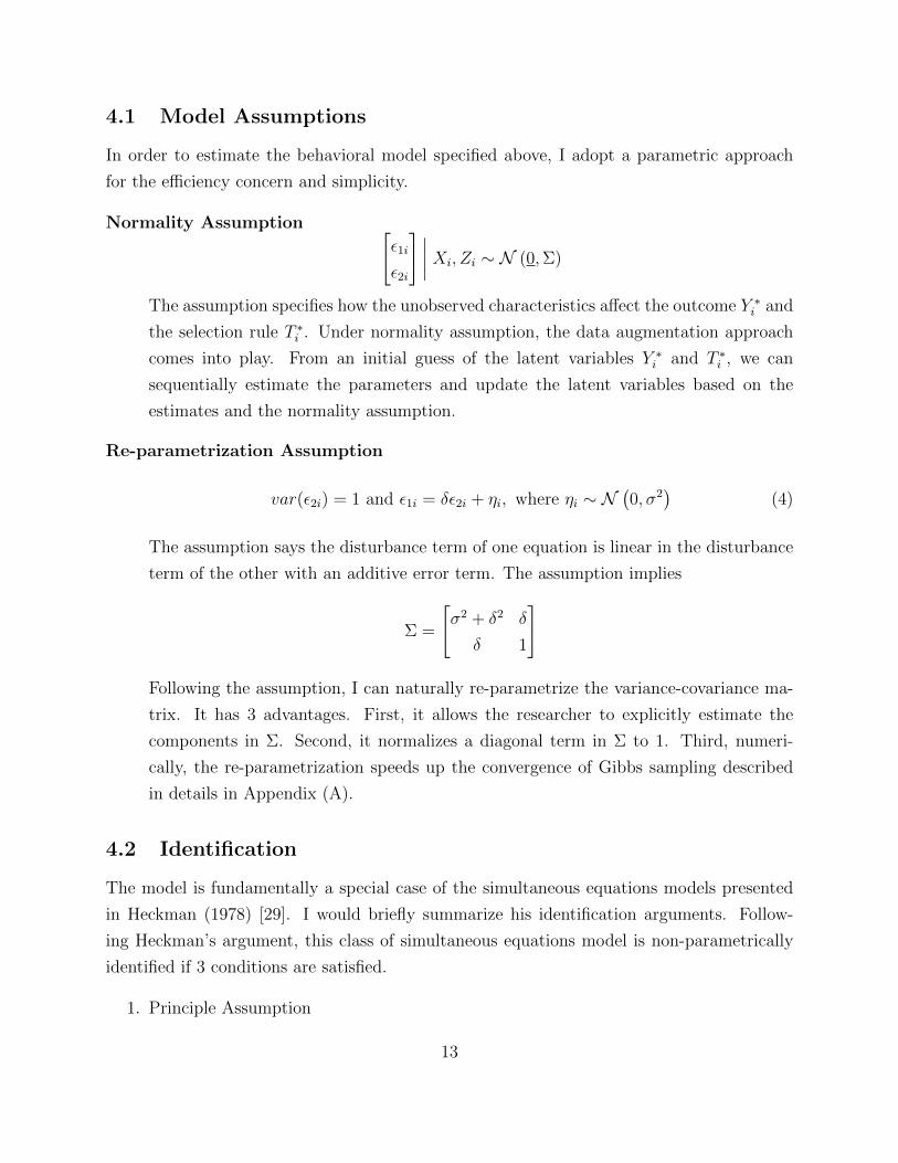
4.1 Model Assumptions

In order to estimate the behavioral model specified above, I adopt a parametric approach

for the efficiency concern and simplicity.

Normality Assumption [ε1i

ε2i

] ∣∣∣∣ Xi, Zi ∼ N (0,Σ)

The assumption specifies how the unobserved characteristics affect the outcome Y ∗i and

the selection rule T ∗i . Under normality assumption, the data augmentation approach

comes into play. From an initial guess of the latent variables Y ∗i and T ∗i , we can

sequentially estimate the parameters and update the latent variables based on the

estimates and the normality assumption.

Re-parametrization Assumption

var(ε2i) = 1 and ε1i = δε2i + ηi, where ηi ∼ N(0, σ2

)(4)

The assumption says the disturbance term of one equation is linear in the disturbance

term of the other with an additive error term. The assumption implies

Σ =

[σ2 + δ2 δ

δ 1

]

Following the assumption, I can naturally re-parametrize the variance-covariance ma-

trix. It has 3 advantages. First, it allows the researcher to explicitly estimate the

components in Σ. Second, it normalizes a diagonal term in Σ to 1. Third, numeri-

cally, the re-parametrization speeds up the convergence of Gibbs sampling described

in details in Appendix (A).

4.2 Identification

The model is fundamentally a special case of the simultaneous equations models presented

in Heckman (1978) [29]. I would briefly summarize his identification arguments. Follow-

ing Heckman’s argument, this class of simultaneous equations model is non-parametrically

identified if 3 conditions are satisfied.

1. Principle Assumption

13

The principle assumption requires that the endogenous variable xi does not enter both

equations. It is a sufficient and necessary condition for the class of simultaneous equa-

tions models to be well-defined. It guarantees we can uniquely solve each parameter

from the equations. My model trivially satisfies the assumption.

2. Normalization of Variance

Given the selection equation has an interpretation as utility, the utility is invariant

to different scaling. The coefficients in the equations are identified up to a constant.

I can normalize a diagonal term of the variance-covariance matrix. I adopt a re-

parametrization approach presented in Section (4.1).

3. Exclusion Restrictions3

Even though I can purely rely on nonlinearity of normality assumption for identifica-

tion, lacking in exclusion restrictions in simultaneous equations models usually hampers

robustness of the estimates.(Manski(1989) [39]) On the other hand, a natural exclusion

restriction is often difficult to find.

Since selection to “cram school” can be interpreted as demand for “cram school,” it

is natural to look for a cost shifter. I follow the insight of Card(1995)[11] to exploit

the geographic variation. The idea is to use the distance between one’s school to

“cram school” to be the exogenous variation. The cost of attending a “cram school”

is composed of the time cost of transportation, the tuition fees, and the time cost the

teenagers spend in the class. As the traveling time to “cram school” increases, the

cost of attending “cram school” rises. Meanwhile, the traveling time does not affect

students’ performance in the admission procedure. It satisfies the exogeneity condition

for an ideal exclusion restriction.

Since I only observe how long it takes the attendants to go to a “cram school” in

the dataset, I estimate a censored regression of commuting time to “cram school” of

the attendants against their family characteristics. I impute the missing commuting

time of the non-attendants using the linear fitted values from the censored regression

estimates. The imputation is valid because students go to school in their school district

in junior high school. Without the rights to driver’s license, junior high students rely

on public transportation, walking, biking, or their parents for mobility. The exam

prep-programs are localized in the school districts. If teenagers with similar family

3I am indebted to Sandeep Shetty for the idea of the exclusion restriction.

14

backgrounds live in a similar neighborhood within the school district, the imputation

based on the fitted value of the censored regression will provide a good approximation

for the missing commuting time for the non-attendants.

4.3 Reference Prior

To complete the Bayesian models, standard normal-gamma conjugate priors are imposed on

the parameters ([24]).

β1 ∼MVN (β01 , σ

2β1I)

τ ∼ N (τ0, σ2τ )

β2 ∼MVN (β02 , σ

2β2I)

δ ∼ N (δ0, σ2δ )

σ2 ∼ IG(a, b)

This is a commonly used proper reference prior, which is an approximation to standard

improper reference prior.(See Christensen(2011)[18]) The parameters on the means of the

normal distributions, β01 , β0

2 , τ , are set to 0. The choice of prior parameters is philosophically

consistent with Zellner (2007) [5] in the sense that all variation is considered random or

nonsystematic unless shown otherwise. I set σ2β, σ2

α, and σ2γ to 106 and set the shape and

scale parameters of the inverse-gamma distribution to 10−3. It gives the inverse gamma

distribution an ε-ε form, which has concentrated density at 0+ and has a long tail. The choice

of theses parameter values are standard. The reference prior corresponding to the standard

frequentist MLE or least squared methods are well-known in the Bayesian literatures, such

as Chib(1992)[15] and Christensen(2011)[18].

4.4 The Results

In Table (6), I present the empirical results estimated by the Bayesian simultaneous equations

model. The first panel shows the results when the outcome is defined as admission to a

public high school. In order to compare the result with the propensity score matching result,

I calculate the average partial effect given treated, P (Y = 1|X, T = 1). Consistent with the

matching estimates, the estimated effect is about 14% increase in the probability of being

admitted to public high school. It also indicates an insignificant negative selection into “cram

school.”

15

The second panel shows the results when the outcome is defined as admission to an “elite”

high school. Conditional on participating in a prep-program, the partial effect of attending

“cram school” increases the chances of being admitted to an “elite” high school by around

6.6%. The estimate is also consistent with matching results. Sorting to “cram school” in

this case is also insignificantly negative.

Table 6: Empirical Results of the Key Variables

Post. Mean Post. SD APE† Post. Mean Post. SD APERegressor Public HS Elite HS

Cram School 1.128∗∗ 0.523 0.107 0.820∗∗∗ 0.208 0.084Minutes to Cram School -0.050∗∗∗ 0.004 - -0.046∗∗∗ 0.004 -

σ2 8.230 1.776 - 2.377 0.470 -δ 0.289 0.327 - -0.153 0.284 -

† The average partial effect of “cram school” is defined conditional on “cram school” attendance when “cramschool” attendance switches from 0 to 1.

∆P̂ (Y = 1|X, T = 1) ≈ 1

N

∑i

φ(Xβ̂)β̂j∆xj

Figure (3) shows the Markov chains and the histograms of the posterior distributions

of treatment effect parameters. The posterior distributions are of standard shape for the

normal-inverse-gamma model. Since both of them are unimodal and symmetric, the 90%

confidence set are simply represented by the 5% and 95% posterior quantiles. I present the

full empirical results in the Appendix.

4.5 Robustness Check

A possible concern about the empirical results may be: Is the result robust in absence of

the Bayesian model? In this section, I implement a standard bivariate Probit model and

compare the results with the Bayesian approach.

Table (7) shows the empirical results using standard bivariate Probit model. Notice that

compared with the Bayesian model developed in the previous section, Probit model imposes

an additional constraint of equal variances. The results indicate that “cram school” raises

students’ chances of being admitted to public high school by 18.8% while it increases their

chances of being admitted to “elite” high school by 3.3%. Both specifications also indicate

slightly negative sorting into “cram school.”

16

0.0

0.2

0.4

0.6

0.8

0 1 2 3

Histogram: Public High School

Cram School

dens

ity

0.0

0.5

1.0

1.5

2.0

2.5

200 400 600 800 1000

Markov Chain: Public High School

Iterations

Cra

m S

choo

l

0.0

0.2

0.4

0.6

0.8

0 1 2

Histogram: Elite High School

Cram School

dens

ity

0.0

0.5

1.0

1.5

2.0

200 400 600 800 1000

Markov Chain: Elite High School

Iterations

Cra

m S

choo

l

Figure 3: Posterior Distributions

† The Markov chains plot every 5 draws of the simulated chains.

Table 7: Robustness Check: Bivariate Probit Model

Post. Mean Post. SD APE† Post. Mean Post. SD APERegressor Public HS Elite HS

Cram School 0.730∗ 0.366 0.220 1.035∗∗ 0.316 0.065Minutes to Cram School -0.051∗∗ 0.005 - -0.047∗∗ 0.005 -

ρ -0.083 0.211 - -0.368∗ 0.205 -

17

4.6 Individual Decision Problem

An advantage of applying Bayesian methods to program evaluation is that it allows the

researchers to think of the problem as a decision problem. (Dehejia(2005)[21]) Imagine a

student wonder whether she should attend “cram school” given her performance in school

and family background. She may be concerned about the uncertainty of the model esti-

mates. The researcher can help her out by exploiting the Bayesian model. The decision

problem for a student to decide whether to enroll in an exam prep-program is associated

with the outcome. It is important to embody the uncertainty of the outcomes from the

model by allowing for parameter uncertainty. The predictive posterior distribution of the

Bayesian model constructs a distribution of outcome based on the posterior distribution of

the parameters.

I simulate the predictive posterior distribution in the following way: for each individual i

in the cohort of interest, say group of family income less than NTD30,000 per month, living

in Taipei City, and having failed a class. Given the covariates Xi as observed, I set T̃ 1i = 1

to simulate for the treated and T̃ 0i = 0 to simulate for the control. Using the stored draws

from the posterior distributions {τ (j), α(j), σ2(j)}5000j=1 , I draw for Y ∗1i |{T̃i, Xi} ∼ N (τ (j) +

Xiα(j), σ2(j)) and Y ∗0i |{T̃i, Xi} ∼ N (Xiα

(j), σ2(j)). Finally, I obtain predicted outcome by

Y 1i = 1(Y ∗1i > 0) and Y 0

i = 1(Y ∗0i > 0).

In Table (8), I show the average predicted probability of being admitted to a public high

school given different levels of family income and whether she has failed a course. I define

low income as earning less than NTD30,000 per month, median income as NTD 50,000 -

NTD 59,999 per month, and high school as earning more than 150,000 per month. The

result shows that the likelihood of being admitted to a public high school is significantly

higher for students from higher income families. Among students who have failed a class, or

less able in academia, the predicted improvement in probability by going to “cram school” is

larger for higher income students than lower income students. However, we do not observe

the same pattern among students who have never failed a class.

Comparing students who fail a class with those who have never failed one, the predicted

effect is also significantly higher for the students who are more able. The effect of “cram

school” for less motivated or less able children is smaller than for motivated and able students.

This suggests that parents should think twice before sending their children who are not

interested in studying to a “cram school” to ”force” them to academic track. The effect may

not outweigh the costs of time, tuition fees, and unnecessary additional pressure.

18

Table 8: Mean and Variance of Predicted Probability of being Admitted to Public HS

Treated Control Treated - ControlCohorts Pred. Prob. S.D. Pred. Prob. S.D. Pred. Diff. S.D. Num. Obs.

Taipei CityLow Income; Fail 0.170 0.376 0.095 0.293 0.075 0.455 111

Median Income; Fail 0.176 0.381 0.099 0.298 0.077 0.466 122High Income; Fail 0.302 0.459 0.189 0.391 0.114 0.575 25

Low Income; Never Fail 0.594 0.491 0.448 0.497 0.146 0.663 36Median Income; Never Fail 0.683 0.465 0.542 0.498 0.141 0.651 69

High Income; Never Fail 0.728 0.445 0.593 0.491 0.134 0.633 26Taipei County

Low Income; Fail 0.110 0.313 0.056 0.230 0.054 0.375 142Median Income; Fail 0.136 0.342 0.070 0.256 0.065 0.415 127

High Income; Fail 0.119 0.324 0.059 0.236 0.060 0.392 20Low Income; Never Fail 0.516 0.500 0.371 0.483 0.145 0.662 46

Median Income; Never Fail 0.534 0.499 0.389 0.487 0.145 0.664 73High Income; Never Fail 0.599 0.490 0.455 0.498 0.145 0.669 9

Yilan CountyLow Income; Fail 0.148 0.355 0.081 0.273 0.067 0.430 90

Median Income; Fail 0.175 0.380 0.098 0.297 0.077 0.464 81High Income; Fail 0.179 0.383 0.103 0.304 0.076 0.467 11

Low Income; Never Fail 0.579 0.494 0.433 0.495 0.146 0.656 18Median Income; Never Fail 0.677 0.468 0.541 0.498 0.136 0.643 36

High Income; Never Fail 0.608 0.488 0.458 0.498 0.150 0.674 5

19

5 Discussions

Exam preparatory programs are prevalent in many East Asian countries because of the

usage of a centrally administered exam system to allocate scarce educational resources.

However, because attendants to these programs may be highly self-selected, there is a lack

of rigorous study on evaluation of the programs. The research question of whether an exam

prep-program increases likelihood of being admitted to a public high school or an “elite”

high school can be motivated by Rosen-Willis life cycle model of human capital investment.

Investment in exam preparatory programs can be considered as a current investment to

decrease future educational costs. We expect “cram school” increases propensity of admission

to a public high school or an “elite” high school.

The paper provides two alternative empirical approaches to evaluate the effectiveness

of “cram schools.” Identification of propensity score matching approach relies on uncon-

foundedness assumption, which states: given the observed characteristics, attending “cram

school” is independent of potential placements. If unconfoundedness assumption holds, then

the average treatment effect on the treated can be obtained by matching each treated unit

with a control unit with the shortest distance in propensity score. The result suggests that

“cram school” increases chances to be admitted to public high school by 16% to 20% and to

“elite” high school by 4% to 7%.

Alternatively, I set up a Bayesian simultaneous equations model that specifies the selec-

tion rule. Identification of the model relies on exogeneity of exclusion restriction. I assume

commuting time from school to “cram school” is relevant to students’ attendance decision and

exogenous to their high school placement. Imposing the constant treatment effect assump-

tion, I can extrapolate the effect of the ”compliers,” who are discouraged from participating

a program due to longer commuting time, to the population of interest. I find evidence that

average partial effect given treated is around 11% in chances of being admitted to a public

high school and 8.4% to an “elite” high school. The result also indicates the correlation of

the unobservable characteristics that affect both selection and outcome is not significantly

different from 0.

The paper adds an important policy perspective to the ongoing debate of educational

reform in Taiwan. The findings suggest that “cram schools” pass the test of the market.

Attending “cram school,” indeed, improves students’ chances to be admitted to a public

high school and an “elite” high school. Even though the Taiwanese policy makers consider

“cram schools” as an unnecessary sources of pressure, these programs will continue to play

an significant role in Taiwanese teenagers’ life without a fundamental change in the centrally

20

administered admission system and the belief of ”elitism.” Whenever there is a demand for

“elite” high school, the market will persist.

References

[1] Alberto Abadie and Guido Imbens. Large sample properties of matching estimators for average treat-

ment effects. Econometrica, 74(1):235–267, 2006.

[2] Joshua D. Angrist. Estimation of limited dependent variable models with dummy endogenous regres-

sors: Simple strategies for empirical practice. Journal of Business & Economic Statistics, 19(1):2–16,

2001. ArticleType: research-article / Full publication date: Jan., 2001 / Copyright c© 2001 American

Statistical Association.

[3] Joshua D. Angrist and Alan Krueger. Empirical strategies in labor economics. In Orley Ashenfelter

and David Card, editors, Handbook of Labor Economics, volume 3. Elsevier Science B.V., 1999.

[4] Zellner Arnold. Bayesian analysis in econometrics. Journal of Econometrics, 37(1):27–50, 1988. doi:

10.1016/0304-4076(88)90072-3.

[5] Zellner Arnold. Philosophy and objectives of econometrics. Journal of Econometrics, 136(2):331–339,

2007. doi: 10.1016/j.jeconom.2005.11.001.

[6] Orley Ashenfelter and Alan Krueger. Estimates of the economic return to schooling from a new sample

of twins. The American Economic Review, 84(5):1157–1173, 1994. ArticleType: research-article / Full

publication date: Dec., 1994 / Copyright c© 1994 American Economic Association.

[7] Gary S. Becker. Investment in human capital: A theoretical analysis. Journal of Political Economy,

70(5):9–49, 1962.

[8] Gary S. Becker. A theory of the allocation of time. The Economic Journal, 75(299), 1965.

[9] Gary S. Becker. Human capital a theoretical and empirical analysis, with special reference to education.

University of Chicago Press, 1993.

[10] Christian Belzil. The return to schooling in structural dynamic models: a survey. European Economic

Review, 51(5):1059–1105, 2007. doi: DOI: 10.1016/j.euroecorev.2007.01.008.

[11] David Card. Using geographic variation in college proximity to estimate the return to schooling. In

Aspects of Labor Market Behaviour: Essays in Honour of John Vanderkamp. Toronto: University of

Toronto Press, 1995.

[12] David Card. Estimating the return to schooling: Progress on some persistent econometric problems.

Econometrica, 69(5):1127–1160, 2001. ArticleType: research-article / Full publication date: Sep., 2001

/ Copyright c© 2001 The Econometric Society.

[13] G. Casella. Empirical bayes gibbs sampling. Biostatistics, 2(4):485–500, 2001.

[14] George Casella and Edward I. George. Explaining the gibbs sampler. The American Statistician,

46(3):167–174, 1992. ArticleType: research-article / Full publication date: Aug., 1992 / Copyright c©1992 American Statistical Association.

21

[15] Siddhartha Chib. Bayes inference in the tobit censored regression model. Journal of Econometrics,

51(1-2):79–99, 1992. doi: 10.1016/0304-4076(92)90030-U.

[16] Siddhartha Chib and Edward Greenberg. Markov chain monte carlo simulation methods in econometrics.

Econometric Theory, 12(3):409–431, 1996. ArticleType: research-article / Full publication date: Aug.,

1996 / Copyright c© 1996 Cambridge University Press.

[17] Siddhartha Chib and Edward Greenberg. Analysis of multivariate probit models. Biometrika, 85(2):347–

361, 1998.

[18] Ronald Christensen. Bayesian ideas and data analysis : an introduction for scientists and statisticians.

CRC Press, Boca Raton, FL, 2011.

[19] Mary Kathryn Cowles and Bradley P. Carlin. Markov chain monte carlo convergence diagnostics: A

comparative review. Journal of the American Statistical Association, 91(434):883–904, 1996. Article-

Type: research-article / Full publication date: Jun., 1996 / Copyright c© 1996 American Statistical

Association.

[20] Rajeev H. Dehejia. Was there a riverside miracle? a hierarchical framework for evaluating programs

with grouped data. Journal of Business & Economic Statistics, 21(1):1–11, 2003. ArticleType: research-

article / Full publication date: Jan., 2003 / Copyright c© 2003 American Statistical Association.

[21] Rajeev H. Dehejia. Program evaluation as a decision problem. Journal of Econometrics, 125(1):141–173,

2005.

[22] B. Efron and R. Tibshirani. Bootstrap methods for standard errors, confidence intervals, and other

measures of statistical accuracy. Statistical Science, 1(1):54–75, 1986. ArticleType: research-article /

Full publication date: Feb., 1986 / Copyright c© 1986 Institute of Mathematical Statistics.

[23] Andrew Gelman. A bayesian formulation of exploratory data analysis and goodness-of-fit testing*.

International Statistical Review, 71(2):369–382, 2003.

[24] Andrew Gelman. Bayesian data analysis. Chapman & Hall/CRC, Boca Raton, Fla., 2004.

[25] Andrew Gelman and Donald B. Rubin. Inference from iterative simulation using multiple sequences.

Statistical Science, 7(4):457–472, 1992. ArticleType: research-article / Full publication date: Nov., 1992

/ Copyright c© 1992 Institute of Mathematical Statistics.

[26] John Geweke, Gautam Gowrisankaran, and Robert J. Town. Bayesian inference for hospital quality in

a selection model. Econometrica, 71(4):1215–1238, 2003.

[27] J. Heckman and V. Joseph Hotz. Choosing among nonexperimental methods for estimating the impact

of social programs: The case of manpower training. Journal of the American Statistical Association,

84(408):862–874, 1989.

[28] James Heckman. Varieties of selection bias. The American Economic Review, 80(2):313–318, 1990.

ArticleType: research-article / Issue Title: Papers and Proceedings of the Hundred and Second Annual

Meeting of the American Economic Association / Full publication date: May, 1990 / Copyright c© 1990

American Economic Association.

22

[29] James J. Heckman. Dummy endogenous variables in a simultaneous equation system. Econometrica:

Journal of the Econometric Society, 46(4):931–959, 1978.

[30] James J. Heckman. Sample selection bias as a specification error. Econometrica, 47(1):153–161, 1979.

ArticleType: research-article / Full publication date: Jan., 1979 / Copyright c© 1979 The Econometric

Society.

[31] Guido W. Imbens and Joshua D. Angrist. Identification and estimation of local average treatment

effects. Econometrica, 62(2):467–475, 1994. ArticleType: research-article / Full publication date: Mar.,

1994 / Copyright c© 1994 The Econometric Society.

[32] Kirabo Jackson. A little now for a lot later: A look at a texas advanced placement incentive program.

The Journal of Human Resources, 45(3):591–639, 2010.

[33] Kirabo Jackson. Do college-prep programs improve long-term outcomes? NBER Working Paper No.

15722, 2012.

[34] Anne O. Krueger. The political economy of the rent-seeking society. The American Economic Review,

64(3):pp. 291–303, 1974.

[35] Kai Li. Bayesian inference in a simultaneous equation model with limited dependent variables. Journal

of Econometrics, 85(2):387–400, 1998. doi: 10.1016/S0304-4076(97)00106-1.

[36] C. Lin. The republic of china (taiwan). In R. M. Thomas and T. W. Postlethwaite, editors, Schooling

in East Asia: Forces of Change, pages 104–35. Pergamon, New York, 1983.

[37] Da-Sen Lin and Yi-Fen Chen. Cram school attendance and college entrance exam scores of senior high

school students in taiwan. Bulletin of Educational Research, 52(4):35 – 70, 2006.

[38] D. V. Lindley and A. F. M. Smith. Bayes estimates for the linear model. Journal of the Royal Statistical

Society. Series B (Methodological), 34(1):1–41, 1972. ArticleType: research-article / Full publication

date: 1972 / Copyright c© 1972 Royal Statistical Society.

[39] Charles F. Manski. Anatomy of the selection problem. The Journal of Human Resources, 24(3):343–360,

1989. ArticleType: research-article / Full publication date: Summer, 1989 / Copyright c© 1989 The

Board of Regents of the University of Wisconsin System.

[40] Andrew D. Martin, Kevin M. Quinn, and Jong Hee Park. MCMCpack: Markov chain monte carlo in

R. Journal of Statistical Software, 42(9):22, 2011.

[41] Tracy L. Regan, Ronald L. Oaxaca, and Galen Burghardt. A human capital model of the effets of

ability and family background on optimal schooling levels. Economic Inquiry, 45(4):712–738, 2007.

[42] Maria L. Rizzo. Statistical computing with R. Chapman & Hall/CRC, Boca Raton, 2008.

[43] Paul R. Rosenbaum and Donald B. Rubin. The central role of the propensity score in observational

studies for causal effects. Biometrika, 70(1):41–55, 1983. 10.1093/biomet/70.1.41.

[44] Peter E. Rossi, Greg M. Allenby, and Robert E. McCulloch. Bayesian statistics and marketing, 2005.

[45] Donald B. Rubin. Matched sampling for causal effects. Cambridge University Press, Cambridge; New

York, 2006.

23

[46] A. F. M. Smith and G. O. Roberts. Bayesian computation via the gibbs sampler and related markov

chain monte carlo methods. Journal of the Royal Statistical Society. Series B (Methodological), 55(1):3–

23, 1993. ArticleType: research-article / Full publication date: 1993 / Copyright c© 1993 Royal Statis-

tical Society.

[47] David Lee Stevenson and David P. Baker. Shadow education and allocation in formal schooling: Tran-

sition to university in japan. American Journal of Sociology, 97(6):1639–1657, 1992. ArticleType:

research-article / Full publication date: May, 1992 / Copyright c© 1992 The University of Chicago

Press.

[48] Martin A. Tanner and Wing Hung Wong. The calculation of posterior distributions by data augmen-

tation. Journal of the American Statistical Association, 82(398):528–540, 1987. ArticleType: research-

article / Full publication date: Jun., 1987 / Copyright c© 1987 American Statistical Association.

[49] R Development Core Team. R: A language and environment for statistical computing, 2011.

[50] Francis Vella. Estimating models with sample selection bias: A survey. The Journal of Human Re-

sources, 33(1):127–169, 1998. ArticleType: research-article / Full publication date: Winter, 1998 /

Copyright c© 1998 The Board of Regents of the University of Wisconsin System.

[51] Greg C. G. Wei and Martin A. Tanner. A monte carlo implementation of the em algorithm and the poor

man’s data augmentation algorithms. Journal of the American Statistical Association, 85(411):699–704,

1990. ArticleType: research-article / Full publication date: Sep., 1990 / Copyright c© 1990 American

Statistical Association.

[52] Robert J. Willis and Sherwin Rosen. Education and self-selection. The Journal of Political Economy,

87(5):S7–S36, 1979.

[53] Arnold Zellner. Bayesian econometrics. Econometrica, 53(2):253–269, 1985. ArticleType: research-

article / Full publication date: Mar., 1985 / Copyright c© 1985 The Econometric Society.

[54] Arnold Zellner and Tomohiro Ando. A direct monte carlo approach for bayesian analysis of

the seemingly unrelated regression model. Journal of Econometrics, 159(1):33–45, 2010. doi:

10.1016/j.jeconom.2010.04.005.

[55] Arnold Zellner and Peter E. Rossi. Bayesian analysis of dichotomous quantal response models. Journal

of Econometrics, 25(3):365–393, 1984. doi: 10.1016/0304-4076(84)90007-1.

24

A Gibbs Sampling Algorithm

The posterior distributions of the parameters of the Bayesian selection models are obtained through Gibbs

Sampling procedure. The Gibbs sampling is a Markov chain Monte Carlo simulation techniques. (Dehejia

(2003)[20]) The algorithm allows me to simulate random variables from a distribution indirectly without

having to calculate its density. A good introductory survey of this method is Casella and George (1992)[14].

The basic idea of Gibbs Sampling is that, by sequentially sampling from the conditional distribution of each

parameter on the remaining parameters, the simulated draws would converge in distribution to a stationary

distribution that is the joint distribution of interest under some regularity conditions. Given the conjugate

priors, all conditional distributions have closed forms. It simplifies the algorithm to sequential drawings from

the following conditionals after I complete the data augmentation steps.

The steps of the Gibbs sampler are as follows4:

Step 1

T ∗i |Ti = 1 ∼ tN[0,∞)

(γzi +Xiβ2 +

δ

σ2 + δ2(Y ∗i − β −Xiβ1),

σ2

σ2 + δ2

)T ∗i |Ti = 0 ∼ tN(−∞,0]

(γzi +Xiβ2 +

δ

σ2 + δ2(Y ∗i −Xiβ1),

σ2

σ2 + δ2

)where tN denotes truncated normal distribution.

Step 2

Y ∗i |Yi = 1 ∼ tN(0,∞)

(τTi +Xiβ1 + δ(T ∗i − γzi −Xiβ2), σ2

)Y ∗i |Yi = 0 ∼ tN(−∞,0)

(τTi +Xiβ1 + δ(T ∗i − γzi −Xiβ2), σ2

)Step 1 and Step 2 are often called ”data augmentation” steps by the seminal work in Tanner and

Wong (1987)[48]. Intuitively, given I observe Ti and the normality assumption on the disturbances, I

can ”observe” the latent variables T ∗i . In addition, given the fixed censored point assumption and the

normality assumption, I can impute the missing values of Y ∗i by drawing from the truncated normal

distribution.

The above argument leads to an algorithm of successive substitution to solve for a fixed point. Nat-

urally, the Gibbs sampling algorithm is ideally applicable.

Step 3

σ2 ∼ IG

(a+

N

2, b+

1

2

[N∑i=1

ε21i − 2δ

N∑i=1

ε1iε2i + δ2N∑i=1

ε22i

])where I denote ε1i = Y ∗i − τ −Xiβ1 and ε2i = T ∗i − γzi −Xiβ2

Step 4

δ ∼ N

(δ0σ

2 + σ2δ

∑Ni=1 ε1iε2i

σ2 + σ2δ

∑Ni=1 ε

22i

,σ2δσ

2

σ2 + σ2δ

∑Ni=1 ε

22i

)4Notice that I suppress the conditionals for simplicity of notations.

25

Step 5 β, α, γ are simulated by Bayesian Regressions:

Notice that I can rearrange Equation (2) and (3):

T ∗i −δ

σ2 + δ2(Y ∗i − τTi −Xiβ1) = γzi +Xiβ2 + ξ2i, where ξ2i ∼ N (0,

σ2

σ2 + δ2)

and

Y ∗i − δ(T ∗i − γzi −Xiβ2) = τTi +Xiβ1 + ξ1i, where ξ1i ∼ N (0, σ2)

To simulate the conditional requires 2 steps. Firstly, notice that the joint normality assumption

immediately leads to [Y ∗iT ∗i

]∼ N

([τTi +Xiβ1

γzi +Xiβ2

],

[σ2 + δ2 δ

δ 1

])By the property of joint normal distribution, I have

E[Y ∗i |T ∗i ] = τTi +Xiβ1 + δ(T ∗i − γzi −Xiβ2)

var[Y ∗i |T ∗i ] = σ2

Now, we can estimate β and α using standard Bayesian regression, which is a special case of Lindley

and Smith (1974)[38]:

Y ∗i − δ(T ∗i − γzi −Xiβ2) = τTi +Xiβ + η1i, where η1i ∼ N (0, σ2)

Secondly, we observe that

E[T ∗i |Y ∗i ] = γzi +Xiβ2 +δ

σ2 + δ2(y∗i − τTi −Xiβ1)

var[T ∗i |Y ∗i ] =σ2

σ2 + δ2

Again, I can estimate γ by standard Bayesian regression5:

T ∗i −δ

σ2 + δ2(Y ∗i − τTi −Xiβ1) = γzi +Xiβ2 + η2i, where η2i ∼ N (0,

σ2

σ2 + δ2)

5In the previous literatures, such as Li (1998)[35], these 2 steps are usually completed by Zellner’s seem-ingly unrelated regressions in one step. Even though these 2 approaches are theoretically equivalent, SURmodel requires computation of the inverse of a sparse matrix of high dimensionality. The approximationerror in the computer routines is likely to slow down the convergence of the chains or even bias the estimates.Considering I do not intend to run a more complex model, such as a multilevel model, the 2-step methodcan be more suitable.

26

B Full Empirical Results

In this section, I report the full empirical results. I obtain all the results by simulating 55000 draws and

discarding the first 5000 draws as the burn-in period. It is a standard procedure in Bayesian estimation to

minimize the impact of the choice of initial points on the simulated posterior distribution. Since I use the

standard normal-gamma model, the posterior distributions are all unimodal so that the 90% high-propensity

confidence set can be easily obtained by looking at 5% and 95% quantiles. I also report the probability that

a parameter is greater than 0 for one-sided significance test. In addition, shrinkage factors are computed

using Gelman-Rubin convergence diagnostics (Cowles (1996)[19] and Gelman et al.(1992)[25]) by simulating

4 parallel chains with initial points disperse around the original initial points. All shrinkage factors in

all specifications are stabilized around 1 implying the convergence of the Markov chains to the stationary

distribution. I do not report the shrinkage factors in the table.

27

Table 9: Bayesian Model: Public High School

Mean SD 5% 25% 50% 75% 95% P(x>0)Equation 1: Public HS

Cram School 1.128 0.523 0.281 0.784 1.120 1.465 2.018 0.985Cram before 0.449 0.322 -0.068 0.230 0.441 0.660 0.984 0.923

male -0.166 0.176 -0.465 -0.281 -0.159 -0.048 0.117 0.167Num. Siblings -0.449 0.132 -0.676 -0.532 -0.442 -0.358 -0.246 0.000

Intention to HS 1.515 0.244 1.136 1.349 1.504 1.665 1.927 1.000less than NTD 30,000 -1.411 0.337 -1.961 -1.637 -1.407 -1.183 -0.864 0.000

NTD 30,000 -NTD 49,999 -0.893 0.316 -1.405 -1.108 -0.891 -0.678 -0.376 0.002NTD 50,000 -NTD 59,999 -1.155 0.327 -1.695 -1.372 -1.150 -0.934 -0.627 0.000NTD 60,000 -NTD 69,999 -0.590 0.390 -1.234 -0.849 -0.585 -0.336 0.042 0.067NTD 70,000 -NTD 79,999 -1.005 0.390 -1.653 -1.270 -0.999 -0.732 -0.371 0.004NTD 80,000 -NTD 89,999 -0.080 0.448 -0.818 -0.380 -0.073 0.217 0.650 0.430NTD 90,000 -NTD 99,999 -0.089 0.438 -0.792 -0.390 -0.097 0.198 0.642 0.411

NTD 100,000 -NTD 109,999 -0.516 0.472 -1.288 -0.836 -0.516 -0.189 0.257 0.141NTD 110,000 -NTD 119,999 -0.748 0.502 -1.560 -1.088 -0.753 -0.409 0.083 0.068NTD 120,000 -NTD 129,999 -1.009 0.580 -1.966 -1.395 -1.011 -0.622 -0.048 0.042NTD 130,000 -NTD 139,999 -0.437 0.682 -1.567 -0.898 -0.440 0.025 0.674 0.262NTD 140,000 -NTD 149,999 0.630 0.760 -0.628 0.112 0.639 1.147 1.886 0.799

more than NTD 150,000 -0.960 0.468 -1.729 -1.269 -0.960 -0.652 -0.199 0.021Sound family -0.055 0.270 -0.506 -0.229 -0.057 0.125 0.388 0.419Fail a subject 3.509 0.372 2.942 3.254 3.484 3.746 4.146 1.000

School FE YesParents’ Educ. YesParents’ Occ. Yes

Equation 2: Cram SchoolCommuting time -0.050 0.004 -0.057 -0.053 -0.050 -0.047 -0.044 0.000

Cram before 1.510 0.065 1.406 1.466 1.508 1.552 1.618 1.000male -0.084 0.061 -0.183 -0.124 -0.084 -0.043 0.017 0.085

Num. Siblings -0.107 0.037 -0.168 -0.132 -0.107 -0.082 -0.046 0.003Intention to HS 0.290 0.068 0.178 0.244 0.289 0.336 0.399 1.000

less than NTD 30,000 0.125 0.220 -0.240 -0.018 0.121 0.269 0.491 0.717NTD 30,000 -NTD 49,999 0.119 0.218 -0.235 -0.027 0.118 0.261 0.482 0.711NTD 50,000 -NTD 59,999 0.140 0.221 -0.220 -0.010 0.137 0.287 0.512 0.736NTD 60,000 -NTD 69,999 0.097 0.237 -0.293 -0.065 0.100 0.253 0.495 0.657NTD 70,000 -NTD 79,999 0.048 0.235 -0.331 -0.106 0.046 0.204 0.446 0.574NTD 80,000 -NTD 89,999 -0.042 0.251 -0.459 -0.208 -0.045 0.123 0.378 0.425NTD 90,000 -NTD 99,999 0.441 0.251 0.026 0.271 0.441 0.611 0.860 0.959

NTD 100,000 -NTD 109,999 -0.109 0.261 -0.534 -0.285 -0.113 0.067 0.321 0.335NTD 110,000 -NTD 119,999 0.007 0.278 -0.447 -0.178 0.004 0.191 0.475 0.505NTD 120,000 -NTD 129,999 0.229 0.319 -0.293 0.012 0.222 0.442 0.768 0.762NTD 130,000 -NTD 139,999 0.005 0.363 -0.596 -0.242 0.005 0.251 0.597 0.506NTD 140,000 -NTD 149,999 -0.235 0.412 -0.904 -0.512 -0.238 0.042 0.447 0.281

more than NTD 150,000 0.127 0.266 -0.309 -0.051 0.124 0.303 0.572 0.686Sound family 0.080 0.100 -0.084 0.012 0.079 0.147 0.245 0.791Fail a subject 0.299 0.071 0.181 0.252 0.300 0.346 0.417 1.000

School FE YesParents’ Educ. YesParents’ Occ. Yes

σ2 8.230 1.776 5.794 6.938 8.006 9.264 11.527 1.000δ 0.289 0.327 -0.261 0.089 0.290 0.506 0.818 0.819

28

Table 10: Bayesian Model: “elite” High School

Mean SD 5% 25% 50% 75% 95% P(x>0)Equation 1: Elite HS

Cram School 0.820 0.208 0.485 0.677 0.819 0.955 1.172 1.000Cram before -0.094 0.269 -0.525 -0.278 -0.100 0.093 0.349 0.366

male -0.056 0.142 -0.289 -0.149 -0.052 0.040 0.167 0.356Num. Siblings -0.320 0.092 -0.480 -0.377 -0.315 -0.258 -0.180 0.000

Intention to HS 0.469 0.189 0.164 0.343 0.464 0.594 0.781 0.993less than NTD 30,000 -1.320 0.334 -1.874 -1.545 -1.324 -1.093 -0.777 0.000

NTD 30,000 -NTD 49,999 -0.838 0.300 -1.333 -1.040 -0.837 -0.632 -0.349 0.002NTD 50,000 -NTD 59,999 -0.824 0.297 -1.317 -1.020 -0.825 -0.628 -0.335 0.004NTD 60,000 -NTD 69,999 -0.366 0.342 -0.930 -0.588 -0.370 -0.143 0.193 0.139NTD 70,000 -NTD 79,999 -0.938 0.347 -1.513 -1.169 -0.934 -0.705 -0.358 0.003NTD 80,000 -NTD 89,999 -0.783 0.391 -1.428 -1.048 -0.776 -0.522 -0.148 0.020NTD 90,000 -NTD 99,999 -0.274 0.365 -0.871 -0.523 -0.278 -0.030 0.327 0.229

NTD 100,000 -NTD 109,999 -0.380 0.404 -1.049 -0.654 -0.367 -0.108 0.283 0.171NTD 110,000 -NTD 119,999 -0.980 0.436 -1.704 -1.274 -0.978 -0.679 -0.264 0.012NTD 120,000 -NTD 129,999 -0.848 0.493 -1.684 -1.170 -0.849 -0.514 -0.042 0.041NTD 130,000 -NTD 139,999 0.197 0.553 -0.720 -0.171 0.193 0.562 1.118 0.643NTD 140,000 -NTD 149,999 -0.703 0.640 -1.738 -1.121 -0.700 -0.277 0.326 0.140

more than NTD 150,000 -0.605 0.381 -1.236 -0.859 -0.600 -0.348 0.026 0.056Sound family -0.336 0.227 -0.711 -0.491 -0.336 -0.182 0.037 0.070Fail a subject 1.984 0.222 1.629 1.834 1.981 2.126 2.344 1.000

School FE YesParents’ Educ. YesParents’ Occ. Yes

Equation 2: Cram SchoolCommuting time -0.046 0.004 -0.053 -0.049 -0.046 -0.043 -0.038 0.000

Cram before 1.509 0.069 1.395 1.462 1.509 1.556 1.623 1.000male -0.034 0.066 -0.142 -0.078 -0.034 0.010 0.075 0.304

Num. Siblings -0.079 0.040 -0.146 -0.106 -0.079 -0.051 -0.012 0.027Intention to HS 0.319 0.074 0.199 0.270 0.320 0.369 0.438 1.000

less than NTD 30,000 0.192 0.228 -0.178 0.037 0.187 0.346 0.568 0.799NTD 30,000 -NTD 49,999 0.133 0.228 -0.239 -0.022 0.129 0.287 0.513 0.724NTD 50,000 -NTD 59,999 0.169 0.229 -0.208 0.012 0.167 0.322 0.553 0.769NTD 60,000 -NTD 69,999 0.234 0.252 -0.170 0.068 0.231 0.398 0.659 0.826NTD 70,000 -NTD 79,999 0.031 0.245 -0.367 -0.141 0.034 0.197 0.435 0.553NTD 80,000 -NTD 89,999 -0.004 0.263 -0.436 -0.177 -0.007 0.177 0.426 0.487NTD 90,000 -NTD 99,999 0.403 0.268 -0.037 0.218 0.405 0.579 0.848 0.935

NTD 100,000 -NTD 109,999 -0.144 0.270 -0.586 -0.329 -0.143 0.041 0.299 0.302NTD 110,000 -NTD 119,999 0.245 0.294 -0.236 0.050 0.245 0.441 0.734 0.800NTD 120,000 -NTD 129,999 0.413 0.343 -0.149 0.177 0.416 0.641 0.978 0.885NTD 130,000 -NTD 139,999 0.105 0.375 -0.507 -0.151 0.100 0.359 0.717 0.606NTD 140,000 -NTD 149,999 -0.081 0.424 -0.788 -0.368 -0.071 0.207 0.592 0.430

more than NTD 150,000 0.136 0.268 -0.304 -0.046 0.134 0.315 0.579 0.691Sound family 0.090 0.107 -0.084 0.018 0.090 0.162 0.270 0.798Fail a subject 0.327 0.078 0.199 0.277 0.327 0.378 0.453 1.000

School FE YesParents’ Educ. YesParents’ Occ. Yes

σ2 2.377 0.470 1.676 2.073 2.331 2.630 3.219 1.000δ -0.153 0.284 -0.628 -0.344 -0.156 0.037 0.323 0.292

29

Table 11: Bivariate Probit Model: Public High School

Variable Coefficient Std. Err. Coefficient Std. Err.Equation 1 : Public HS Equation 2 : Cram School

Cram School 0.730∗ 0.366 - -Commuting time - - -0.051∗∗ 0.005Cram before 0.021 0.196 1.494∗∗ 0.082Male 0.016 0.060 -0.080 0.079Num. Siblings -0.043 0.049 -0.103∗∗ 0.029less than NTD 30,000 -0.761 0.524 -0.072 0.311NTD 30,000 -NTD 49,999 -0.560 0.538 -0.076 0.289NTD 50,000 -NTD 59,999 -0.663 0.539 -0.062 0.288NTD 60,000 -NTD 69,999 -0.503 0.556 -0.106 0.307NTD 70,000 -NTD 79,999 -0.641 0.535 -0.152 0.332NTD 80,000 -NTD 89,999 -0.286 0.539 -0.252 0.335NTD 90,000 -NTD 99,999 -0.313 0.575 0.249 0.307NTD 100,000 -NTD 109,999 -0.475 0.511 -0.306 0.325NTD 110,000 -NTD 119,999 -0.585 0.546 -0.174 0.327NTD 120,000 -NTD 129,999 -0.793 0.572 0.034 0.327NTD 130,000 -NTD 139,999 -0.514 0.600 -0.201 0.424NTD 140,000 -NTD 149,999 0.397 0.655 -0.450 0.405more than NTD 150,000 -0.639 0.549 -0.075 0.345Sound family 0.128 0.094 0.062 0.094Intention to HS 0.617∗∗ 0.079 0.295∗∗ 0.073Fail a subject 1.288∗∗ 0.092 0.303∗∗ 0.090School FE YesParents’ Educ. YesParents’ Occ. Yesρ -0.083 0.211

30

Table 12: Bivariate Probit Model: “elite” High School

Variable Coefficient Std. Err. Coefficient Std. Err.Equation 1 : Elite HS Equation 2 : Cram School

Cram School 1.035∗∗ 0.316 - -Commuting time - - -0.047∗∗ 0.005Cram before -0.251 0.172 1.486∗∗ 0.087Male 0.039 0.075 -0.043 0.084Num. Siblings -0.077 0.065 -0.080∗∗ 0.030less than NTD 30,000 -2.339∗∗ 0.474 0.466 0.402NTD 30,000 -NTD 49,999 -2.076∗∗ 0.480 0.417 0.378NTD 50,000 -NTD 59,999 -2.041∗∗ 0.473 0.448 0.371NTD 60,000 -NTD 69,999 -1.774∗∗ 0.436 0.501 0.411NTD 70,000 -NTD 79,999 -2.125∗∗ 0.443 0.304 0.413NTD 80,000 -NTD 89,999 -2.074∗∗ 0.477 0.267 0.412NTD 90,000 -NTD 99,999 -1.670∗∗ 0.481 0.677† 0.376NTD 100,000 -NTD 109,999 -1.789∗∗ 0.439 0.122 0.395NTD 110,000 -NTD 119,999 -2.298∗∗ 0.499 0.551 0.432NTD 120,000 -NTD 129,999 -2.200∗∗ 0.535 0.710† 0.422NTD 130,000 -NTD 139,999 -1.365∗∗ 0.506 0.402 0.513NTD 140,000 -NTD 149,999 -2.253∗∗ 0.643 0.187 0.499more than 150,000 -1.886∗∗ 0.490 0.398 0.392Sound family -0.104 0.127 0.058 0.110Intention to HS 0.426∗∗ 0.138 0.317∗∗ 0.074Fail a subject 1.391∗∗ 0.154 0.319∗∗ 0.101School FE YesParents’ Educ. YesParents’ Occ. Yesρ -0.368† 0.205

31