Cramer-Rao Bounds for Joint RSS/DoA-Based Primary-User Localization in Cognitive Radio Networks

IEEE TRANSACTIONS ON WIRELESS COMMUNICATIONS, VOL. 12, NO. 3, MARCH 2013 1363

Cramer-Rao Bounds for Joint RSS/DoA-BasedPrimary-User Localization in

Cognitive Radio NetworksJun Wang, Student Member, IEEE, Jianshu Chen, Student Member, IEEE, and Danijela Cabric, Member, IEEE

Abstract—Knowledge about the location of licensed primary-users (PU) could enable several key features in cognitive radio(CR) networks including improved spatio-temporal sensing, in-telligent location-aware routing, as well as aiding spectrum policyenforcement. In this paper we consider the achievable accuracyof PU localization algorithms that jointly utilize received-signal-strength (RSS) and direction-of-arrival (DoA) measurements byevaluating the Cramer-Rao Bound (CRB). Previous works evalu-ate the CRB for RSS-only and DoA-only localization algorithmsseparately and assume DoA estimation error variance is a fixedconstant or rather independent of RSS. We derive the CRBfor joint RSS/DoA-based PU localization algorithms based onthe mathematical model of DoA estimation error variance asa function of RSS, for a given CR placement. The bound iscompared with practical localization algorithms and the impactof several key parameters, such as number of nodes, number ofantennas and samples, channel shadowing variance and correla-tion distance, on the achievable accuracy are thoroughly analyzedand discussed. We also derive the closed-form asymptotic CRBfor uniform random CR placement, and perform theoretical andnumerical studies on the required number of CRs such that theasymptotic CRB tightly approximates the numerical integrationof the CRB for a given placement.

Index Terms—Cognitive radio, localization, Cramer-Raobounds.

I. INTRODUCTION

COGNITIVE Radio (CR) is a promising approach toefficiently utilize the scarce RF spectrum resources [1].

In this paradigm, knowledge about spectrum occupancy intime, frequency, and space that is both accurate and timelyis crucial in allowing CR networks to opportunistically usethe spectrum and avoid interference to a primary user (PU)[2]. In particular, information about PU location could enableseveral key capabilities in CR networks including improvedspatio-temporal sensing, intelligent location-aware routing, aswell as aiding spectrum policy enforcement [3].

The PU localization problem in CR networks is in gen-eral different from localization in other applications such asWireless Sensor Networks (WSN) [4] and Global PositioningSystem (GPS) [5], due to the following two features. First, aPU does not cooperate or communicate with CRs since theyare opportunistic users of the PU spectrum band. Therefore,

Manuscript received July 2, 2012; revised October 9 and November 29,2012; accepted December 14, 2012. The associate editor coordinating thereview of this paper and approving it for publication was C. Tellambura.

The authors are with the Department of Electrical Engineering, Universityof California, Los Angeles, CA, 90095, USA (e-mail: {eejwang, jshchen,danijela}@ee.ucla.edu).

This work is supported by the National Science Foundation under GrantNo.1117600.

Digital Object Identifier 10.1109/TWC.2013.012513.120966

very limited knowledge about PU signaling, such as transmitpower or modulation scheme, is available to CRs. As a result,passive localization techniques should be applied. Second,since CRs need to detect and localize PUs in the wholecoverage area at a very low signal-to-noise ratio (SNR),in order to avoid interference to the primary network, therequired number of CRs is relatively large and cooperationamong CRs is necessary.

A. Related Work

Prior research on passive localization can be categorizedinto three classes based on the types of measurements sharedamong sensors to obtain location estimates [4]. Received-signal-strength (RSS) based algorithms use measured receivedpower from the PU to provide coarse-grained estimates ata low hardware and computational cost. Time-difference-of-arrival (TDoA) based algorithms obtain location estimatesfrom time differences among multiple receptions of the trans-mitted signal. They are not suitable for CR applicationssince TDoA-based algorithms require perfect synchronizationamong CRs. Direction-of-arrival (DoA) based algorithms usetarget DoA estimates observed at different receivers to obtainlocation estimates. The DoA estimates can be obtained fromeither multiple antenna arrays, directional antennas or virtualarrays formed by cooperative CRs. Therefore, RSS and DoA-based algorithms are the proper choices for the PU localizationproblem.

Passive localization based on RSS and/or DoA measure-ments has been well-studied in both WSN and CR litera-ture, in terms of algorithm design and evaluation. RSS-basedalgorithms include range-based and range-free techniques, adetailed survey can be found in [6]. Popular DoA fusionalgorithms include Maximum Likelihood (ML) [7], Stansfieldalgorithm [8] and Linear Least Square (LLS), each of whichprovides different tradeoff between accuracy and complexity.Algorithms that jointly utilize RSS and DoA informationare also proposed. For example, weighted versions of thepopular DoA fusion algorithms are shown to improve thelocalization accuracy [7]. The weights are typically estimatederror variances of individual DoA measurements, that areobtained from instant RSS [9]. Bayesian approaches, such asKalman filtering and particle filtering, can also be used to fuseRSS and/or DoA measurements [10].

In this paper, we focus on characterizing the achievableperformance of joint RSS/DoA-based localization algorithmsby means of the Cramer-Rao Bound (CRB), which providesa lower bound on the estimation accuracy of any unbiasedestimator using either or both RSS and DoA. The CRB for

1536-1276/13$31.00 c© 2013 IEEE

1364 IEEE TRANSACTIONS ON WIRELESS COMMUNICATIONS, VOL. 12, NO. 3, MARCH 2013

RSS-only localization is studied in [4] and [11] assuming inde-pendent and correlated shadowing channel, respectively. TheDoA-only CRB is discussed in several papers [4], [12]–[15],however they all assume the DoA estimates from different CRsare subject to i.i.d. Gaussian errors with zero mean and fixedvariance. Since the DoA estimation error variance dependson instant RSS and other system parameters (e.g. number ofantennas and samples, array orientation error) [9], assumingit’s constant makes the derived bounds less accurate. Recently,the mathematical model of DoA estimation error is used in[16]–[18] to calculate DoA estimation error variance for somespecific system settings, such as node density and placement,using fixed value of RSS for all CRs. The variance values arethen plugged into the existing DoA-only CRB to evaluate thelocalization performance. This approach does not include thesystem parameters in the mathematical model of DoA errorvariance and channel parameters in RSS, thus the CRB is lesscomprehensive.

B. Contributions

Since the DoA estimation accuracy strongly depends onRSS, and practical algorithms show that using both RSS andDoA estimates provides better localization accuracy than usingDoA alone, the CRB for joint RSS/DoA-based localization ismore capable to characterize the positioning ability of the CRnetwork. Along this direction, this paper has the followingcontributions:

1) Derivation of the CRB for joint RSS/DoA-based passivelocalization considering the interdependency betweenRSS and DoA, for a given CR placement. The CRBis derived for both optimal DoA estimation algorithm,with error given by the CRB of DoA estimation errorvariance, and MUSIC algorithm. Therefore, the derivedCRB provides both ultimate achievable accuracy andthe accuracy achieved by a practical DoA estimationalgorithm.

2) Derivation of closed-form asymptotic joint RSS/DoA-based CRB for uniform random CR placement withi.i.d shadowing. The asymptotic RSS-only CRB forsuch case is also derived as a byproduct. We alsoprovide theoretical and numerical studies on the requirednumber of CRs that ensures the asymptotic CRB tightlyapproaches the numerical integration of the CRB for agiven placement.

3) Study of the impact of various system, channel and arrayparameters on the localization accuracy, theoreticallyand via simulation. The considered parameters includenumber of CRs, CR placement, shadowing variance,correlation distance, number of antennas, number ofsamples and array orientation error. The study providesinsights and guidelines for practical system design ofPU localization in CR network.

4) Comparison of the derived CRBs with practical RSS-only, DoA-only and joint RSS/DoA localization algo-rithms. We study the robustness of practical algorithmsto major system parameters, and reveal the potentialimprovements of practical localization system and al-gorithm design.

The rest of the paper is organized as follows. The systemmodel is introduced in Section II. The joint CRB derivationfor a fixed CR placement is presented in Section III. Theasymptotic joint CRB derivation for uniform CR placement isshown in Section IV. Numerical results evaluating impacts ofvarious parameters on the joint CRB are discussed in SectionV. Finally, the paper is concluded in Section VI.

II. SYSTEM MODEL

Assume N CRs cooperate to localize a single PU. 2-dimensional locations of the PU and the nth CR are denotedas �P = [xP , yP ]

T and �n = [xn, yn]T , respectively. All

locations are static in the observation period, and CR locationsare known. Available measurements at CRs are RSS andDoA. RSS measurement at the nth CR is modeled as ψn �PT

c010−sn/10

dγnWatt, where PT is the PU transmit power, c0 is

the (constant) average multiplicative gain at reference distance,dn = ‖�n−�P ‖ is the distance between the nth CR and PU, γis the path loss exponent, and 10−sn/10 is a random variablethat reflects shadowing. The RSS is normally expressed indBm using the transformation φn = 10 log10(1000ψn), theresult is given as

φn = 10 log10(1000PT c0)−10γ log10 dn−sn � φn−sn. (1)

Denote collection of RSS measurements from all CRs asφ = [φ1, φ2, . . . , φN ]T . The conditional distribution of φ (fora given �P ) is φ ∼ N (φ,Ωs), where φ = [φ1, φ2, . . . , φN ]T ,and Ωs is the covariance matrix of the collections of the shad-owing variables s = [s1, s2, . . . , sN ]T given by {Ωs}mn =σ2se

−‖�m−�n‖/Xc , where Xc is the correlation distance withinwhich the shadowing effects among nodes are correlated.

The DoA of the PU at the nth CR is given as θn �arctan( yP−yn

xP−xn) � ∠(�P , �n). CRs perform array signal pro-

cessing techniques, such as MUSIC [19] or ESPRIT [20],to obtain DoA estimates. The estimated DoA is commonlymodeled as θn � θn + vn [9], where vn ∼ N (0, σ2

n) andσ2n is the DoA estimation error variance. We denote θ =

[θ1, θ2, . . . , θN ] as collections of DoA measurements of allCRs at the fusion center. We consider two different modelingsof the DoA estimation error variance, using CRB and MUSICalgorithm, respectively. The CRB of DoA estimation errorvariance for unbiased DoA estimators using arbitrary arrayresponse is presented in [9, Sec. IV, Eqn. 4.1], the result forUniform Linear Array (ULA) is given by [17, Sec. III-B, Eqn.20]

σ2n,CRB =

1

(κ cos θn)2

6

NsNa(N2a − 1)ρn

, (2)

where κ is a constant determined by the signal wavelengthand array spacing, Ns is the number of samples, Na is thenumber of antennas, θn is the array orientation with respectto the incoming DoA defined as θn � θn − θn, where θnis the orientation of the nth ULA, and ρn is the signal-to-noise (SNR) ratio given by ρn = ψn/PM , where PM is themeasurement noise power. Using the definition of SNR wecan simplify (2) as

σ2n,CRB =

6PMκ2NsNa(N2

a − 1)

1

ψn

1

cos2 θn

= βfCRB(φn)1

cos2 θn. (3)

WANG et al.: CRAMER-RAO BOUNDS FOR JOINT RSS/DOA-BASED PRIMARY-USER LOCALIZATION IN COGNITIVE RADIO NETWORKS 1365

where β � 6PM

κ2NsNa(N2a−1) and fCRB(φn) � 1

ψn. The DoA

estimates from MUSIC are, asymptotically in the sample size,unbiased and Gaussian distributed with error variance givenby [9, Sec. III-B, Eqn. 3.11]. The estimation error varianceusing ULA is given by [17, Sec. III-B, Eqn. 21]

σ2n,MU =

1

(κ cos θn)2

6

NsNa(N2a − 1)ρn

(1 +1

Naρn)

= βfMU (φn)1

cos2 θn. (4)

where fMU (φn) � ψn+(PM/Na)ψ2n

. Note that both (3) and (4)

depend on RSS and PU location (used in calculation of θn).The PU localization problem uses RSS and DoA measure-

ments to obtain PU location estimate �P � [xp, yp]T . The

Root-Mean-Square-Error (RMSE) of the location estimates

is given by RMSE �√E

[‖�P − �P ‖2

]. A brief table

of notations used in the paper is given in Table I. Notethat we assume narrowband signals from far-field transmitterspropagated via a single-path channel, thus DoA measurementand fusion are possible and practical. In the narrowband far-field scenario, RSS readings from each antenna are the sameand they cannot be used to obtain DoA estimates. In suchcase, array processing techniques, such as MUSIC, use phaseinformation from the array to obtain DoA estimates, and theRSS determines the statistical DoA estimation quality as canbe seen from (3) and (4). For the case when the transmitteris in near-filed or the wireless channel has significant multi-path, DoA measurement is not reliable and the CRB derivationshould start from the raw measurement data of the antennaarrays [16], [21] which is beyond the scope of this work.

III. JOINT CRBS FOR FIXED CR PLACEMENT

In this section we derive the joint CRB and the correspond-ing bound on RMSE for a fixed CR placement, for DoAestimates obtained from both optimal estimator and MUSICalgorithm. We also derive the CRB and RMSE for RSS-only localization as a byproduct. Using RSS and DoA asmeasurements, the covariance matrix of unbiased estimationof PU locations �P is lower-bounded by the CRB

Ω�P

� E

[(�P − E

[�P

])(�P − E

[�P

])T]≥ F−1, (5)

where F is the 2 × 2 Fisher Information Matrix (FIM) givenby

F = −Eθ,φ

[∂2

∂�2Plog p(θ, φ|�P )

]. (6)

Therefore the RMSE is bounded by RMSE ≥√{F−1}11 + {F−1}22, where {X}ij denotes the ijth

element of matrix X. Using the standard decomposition ofconditional probability p(θ, φ|�P ) = p(θ|φ, �P )p(φ|�P ), theFIM is decomposed as

F =

{−E

θ,φ

[∂2

∂�2Plog p(θ|φ, �P )

]}+

{−E

φ

[∂2

∂�2Plog p(φ|�P )

]}� F

θ|φ + Fφ. (7)

Note that Fφ is the FIM for using only RSS to localize the

PU, therefore its inverse bounds the localization accuracy ofalgorithms that only use RSS readings. In the rest of thesection, we first derive the RSS-only FIM F

φ. We then presentthe results for the joint FIM F by deriving F

θ|φ for optimalDoA estimator and MUSIC algorithm, respectively.

A. RSS-only CRB

To derive the RSS-only FIM Fφ, we first explicitly express

the logarithm of the PDF of φ

log p(φ|�P ) = − log[(2π)N/2(detΩs)

1/2]

−1

2(φ− φ)TΩ−1

s (φ− φ). (8)

The RSS-only FIM Fφ is then given by

Fφ =

1

2E

φ

[∂2

∂�2P(φ− φ)TΩ−1

s (φ− φ)

](9)

The elements of Fφ are derived as

{Fφ

}11

=∂(φ− φ)T

∂xPΩ−1

s∂(φ− φ)

∂xP= εγ2ΔxTD−2Ω−1

s D−2Δx{Fφ

}22

=∂(φ− φ)T

∂yPΩ−1

s∂(φ− φ)

∂yP= εγ2ΔyTD−2Ω−1

s D−2Δy{Fφ

}12

={

Fφ

}21

=∂(φ− φ)T

∂xPΩ−1

s∂(φ− φ)

∂yP= εγ2ΔxTD−2Ω−1

s D−2Δy, (10)

where ε = 100/(log 10)2, and vectors and matrices are definedas D � diag(d1, d2, . . . , dN ), Δx � [Δx1,Δx2, . . . ,ΔxN ]T ,Δy � [Δy1,Δy2, . . . ,ΔyN ]T , and Δxn = xP − xn andΔyn = yP − yn. Detailed derivations are provided in Ap-pendix A. To obtain a compact expression of F

φ, let’s defineL = [Δx,Δy]T and Λ = 1

εγ2 D2ΩsD2. Therefore, it is

straightforward to verify that the FIM and RMSE of RSS-only PU localization are given by

Fφ = LΛ−1LT

RMSER,F ≥√{F−1

φ}11 + {F−1

φ}22, (11)

where the subscript R,F stands for RSS-only bound for fixedplacement.

B. Joint CRB using Optimal DoA Estimator

In this subsection we derive the joint CRB with DoAestimations given by the optimal estimator, using the DoAerror variance given by σ2

n,CRB . To derive the conditional FIMof DoA given RSS F

θ|φ, we first explicitly express logarithm

of the conditional PDF p(θ|φ, �P ) as


TABLE ISUMMARY OF VARIABLES USED IN THIS PAPER

Symbol Meaning Typical Value

N , n number of CRs, index of CRs 10-100, –R, R0 radius of: PU coverage area, guard region 150m, 5m

�n = [xn, yn]T 2-dimensional coordinate of the nth CR Uniform�P = [xP , yP ]T 2-dimensional coordinate of the PU [0,0]�P = [xP , yP ]T Estimated 2-dimensional coordinate of the PU –dn, Δxn, Δyn distance from the nth CR to the PU, distance on x-axis, distance on y-axis –PT , PM , ρn PU transmit power, measurement noise power, received SNR 20dBm, -80dBm, 10dB

c0, γ channel multiplicative gain at reference distance, path-loss exponent 1, 5sn, σ2s , Xc shadowing variable, its variance, correlation distance –, 6dB, 15mΩ

�P, Ωs Covariance matrix of: the PU location estimates, shadowing variables –, –

ψn, φn, φn RSS measurement: in Watt, in dBm, mean in dBm –, –, –θn, θn incoming DoA and its estimate –, –

θn, θn, θT ULA orientation, orientation error and its distribution parameter –, –, π/3Ns, Na, κ ULA parameters: number of samples, number of antennas, array constant 50, 2, π/2

σ2n,CRB , σ2n,MU DoA error variance of the nth CR given by: CRB, MUSIC algorithm –, –Fφ

, Fθ|φ, F FIM for: RSS-only, DoA given RSS, joint RSS/DoA scenarios –, –, –

α, β, ε supporting constants: α � c0PT eσ2s/(2ε)

β, β � 6PM

κ2NsNa(N2a−1)

, ε � 100(log 10)2

3.2e12, 8.1e-14,18.86

δ0, η deviation distance and corresponding probability used in Theorem 1 and 2 –, 0.15s, φ, θ vector form of: shadowing variables, RSS in dBm, DoA estimates –, –, –

log p(θ|φ, �P ) = log

⎧⎨⎩N∏

n=1

1√2πσ2

n,CRB

exp

[− (θn − θn)

2

2σ2n,CRB

]⎫⎬⎭=

N∑n=1

{log(cos θn)− 1

2log

[2πβfCRB(φn)

]− cos2 θn(θn − θn)

2

2βfCRB(φn)

}. (12)

Then Fθ|φ is given by

Fθ|φ =

N∑n=1

{Eθ,φ

[∂2gn

∂�2P

]− E

θ,φ

[∂2hn

∂�2P

]}(13)

where gn � cos2 ˜θn(θn−θn)22βfCRB(φn)

and hn � log(cos θn). Theelements of F

θ|φ are derived as

{Fθ|φ

}11

=N∑n=1

Δy2nd4n

{α cos2 θn

dγn+ 2 tan2 θn

}{

Fθ|φ

}22

=N∑n=1

Δx2nd4n

{α cos2 θn

dγn+ 2 tan2 θn

}{

Fθ|φ

}12

= −N∑n=1

ΔxnΔynd4n

{α cos2 θn

dγn+ 2 tan2 θn

}.(14)

and{

Fθ|φ

}21

={

Fθ|φ

}12

, where α � c0PT eσ2s/(2ε)/β.

Detailed derivations are provided in Appendix A. To ob-tain a compact expression of F

θ|φ, let’s define P =

[Δy,−Δx]T and Γ = diag(γ1, γ2, . . . , γN ), where γn =1d4n

{α cos2 ˜θn

dγn+ 2 tan2 θn

}. Then it is straightforward to ver-

ify that Fθ|φ = PΓPT . Therefore, the joint FIM and the

corresponding RMSE are given by

FJ,F,C = PΓPT + LΛ−1LT

RMSEJ,F,C ≥√{F−1

J,F,C}11 + {F−1J,F,C}22

(15)

where the subscript J, F, C represents joint CRB for fixedplacement using CRB of DoA estimation error variance.

C. Joint CRB using MUSIC Algorithm

In this section we derive the joint CRB with DoA estima-tions given by the MUSIC algorithm, using the error variancegiven by σ2

n,MU . The conditional FIM of DoA given RSS

Fθ|φ is derived by replacing fCRB(φn) in (12) with fMU (φn)

given by (4). Applying the results in Appendix A, we obtainFθ|φ = PΔPT , where Δ = diag(δ1, δ2, . . . , δN ) and

δn =1

d4n

{cos2 θnβ

[c0PT e

σ2s/(2ε)

dγn− PMNa

+P 2M

N2a

Eφ

(1

ψn + PM

Na

)]+ 2 tan2 θn

}. (16)

Since the RSS-only FIM is independent of DoA estimationalgorithm, the joint FIM and the corresponding RMSE usingMUSIC algorithm are given by

FJ,F,M = PΔPT + LΛ−1LT

RMSEJ,F,M ≥√{F−1

J,F,M}11 + {F−1J,F,M}22, (17)

where the subscript J, F,M represents joint CRB for fixedplacement using MUSIC error variance. Note that the abovecalculations are based on a particular fixed node placement.If the nodes are randomly placed within the area according tosome distribution, say uniform distribution, integrating RMSEexpressions in (11), (15) and (17) for 2N times over all nodecoordinates gives the theoretical average performance bound.

IV. ASYMPTOTIC JOINT CRB FOR UNIFORM RANDOM CRPLACEMENT

The bounds on RMSE derived in Section III are useful toevaluate the achievable localization performance for a givenCR placement. Numerical integration or ensemble averaging


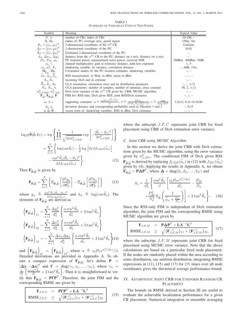
Fig. 1. Illustration of the PU-centric circular model of CR placement.

need to be performed to get the average accuracy for randomCR placements. In this section we characterize the achievablelocalization accuracy for the most common random placement,i.e. the uniform random placement, by deriving the closed-form asymptotic CRB for such case, assuming i.i.d. shadowingand optimal DoA estimator. We also provide theoretical anal-ysis on the required number of CRs as a function of systemparameters to make the asymptotic bound tight.

We assume the CRs that can hear the PU form a circlewith radius R and are uniformly placed in the area, as shownin Fig.1. The CRs are placed independently within the area,which indicates independency among all θn’s, all dn’s, andpairs of θn and dn. For this scenario, the distribution of θn isgiven by θn ∼ U [0, 2π), and the distribution of dn is derivedas

pdn(r) =

⎧⎨⎩2r

(R2 −R20), R0 ≤ r ≤ R (18a)

0, otherwise, (18b)

where R0 is a guard distance to avoid overlap between CRsand PU. Detailed derivation of pdn(r) is shown in AppendixB. We further assume the array orientation error is distributedas θn = θn − θn ∼ U(−θT , θT ), which means the arrayorientation is uniformly distributed around the incoming DoAwith parameter θT .

A. Asymptotic RSS-only CRB

For the RSS-only FIM Fφ with i.i.d. shadowing, we first

rewrite it from (10) as

1

NFφ =

εγ2

σ2sN

N∑n=1

d−2n

[cos θnsin θn

][cos θn, sin θn], (19)

in which we use the fact that [Δxn,Δyn] =[dn cos θn, dn sin θn]. From (19) we observe that 1

N Fφ

can be interpreted as the ensemble average of a function ofrandom variables dn and θn, with statistical mean given by

1

NE

[Fφ

]=εγ2

2σ2s

Edn [d−2n ]I2 =

εγ2 log(R/R0)

σ2s (R

2 −R20)

I2

� fφ(R, γ, σ

2s)I2, (20)

where we obtain the first equality from (19)based on the i.i.d. distribution of dn and θn, andEθn

{[cos θn, sin θn]

T [cos θn, sin θn]}

= 12 I2, where I2

is a 2 × 2 identity matrix. The deviation probability of the

ensemble average 1N F

φ from the statistical mean 1N E

[Fφ

]is given by the following theorem.

Theorem 1: (Deviation Probability of RSS-only FIM) Forany δ0 > 0, we have

Pr

{∥∥∥∥ 1

NFφ − 1

NE

[Fφ

]∥∥∥∥F

> δ0

}<

2ε2γ4

σ4sδ

20N

[1

2R2R20

− log2(R/R0)

(R2 −R20)

2

], (21)

where ‖·‖ represents Frobenius matrix norm.The proof of the theorem is based on Chebyshev’s in-

equality for random matrix, and all details are provided inAppendix C. The intuition from Theorem 1 is that we canwell-approximate 1

N Fφ with 1

N E

[Fφ

]when N is large

enough. In order for the deviation probability to be smallerthan a pre-defined threshold η ∈ (0, 1), we need to bound theright-hand-side of (21) by η. The required number of CRs isthen bounded by

N ≥ 2ε2γ4

σ4sδ

20η

[1

2R2R20

− log2(R/R0)

(R2 −R20)

2

]. (22)

Applying the approximation, the RMSE of RSS-only algo-rithms for uniform random CR placement is given by

RMSER,U ≥(

2

Nfφ(R, γ, σ

2s)

)1/2

, (23)

where the subscript R,U represents RSS-only CRB for uni-form placement.

B. Asymptotic Joint CRB

We apply similar procedure in Sec. IV-A to derive theasymptotic joint CRB from F = F

φ + Fθ|φ. We first rewrite

Fθ|φ from (14) as

1

NFθ|φ =

1

N

N∑n=1

{[αd−(γ+2)

n cos2 θn + 2d−2n tan2 θn

]×

[sin θn

− cos θn

][sin θn,− cos θn]

}. (24)

From (24) we observe that 1N F

θ|φ can be interpreted as theensemble average of a function of random variables dn, θnand θn, with statistical mean given by

1

NE

[Fθ|φ

]=

1

(R2 −R20)

[2 log(R/R0)

(tan θTθT

− 1

)− α

2γ(R−γ −R−γ

0 )

(sin 2θT2θT

+ 1

)]I2,

= fθ|φ(R, γ, σ

2s , θT , β)I2. (25)

The deviation probability of the ensemble average 1N F from

the statistical mean 1N E [F] = 1

N E

[Fφ

]+ 1

N E

[Fθ|φ

]is

given by the following theorem.Theorem 2: (Deviation Probability of Joint FIM) For any

δ0 > 0, the deviation probability of the joint FIM is given by(26) at the top of the page, where fn � αd

−(γ+2)n cos2 θn +


Pr

{∥∥∥∥ 1

NF − 1

NE [F]

∥∥∥∥F

> δ0

}<

1

Nδ20

{ε2γ4

σ4sR

2R20

+ E[f2n

]− 1

2

[E [fn] +

2εγ2 log(R/R0)

σ2s(R

2 −R20)

]2}(26)

E[f2n

]=

4 tan5 θT5θTR2R2

0

× 2F1

(5

2, 1,

7

2,− tan2 θT

)−

2α(R−(γ+2) −R

−(γ+2)0

)(γ + 2)(R2 −R2

0)

(2− sin 2θT

θT

)

−α2 (sin 4θT + 8 sin 2θT + 36θT )

[R−2(γ+1) −R

−2(γ+1)0

]32θT (γ + 1)(R2 −R2

0)(27)

N ≥ 1

ηδ20

{ε2γ4

σ4sR

2R20

+ E[f2n

]− 1

2

[E [fn] +

2εγ2 log(R/R0)

σ2s(R

2 −R20)

]2}(28)

RMSEJ,U,C ≥⎧⎨⎩ 2

N[fφ(R, γ, σ

2s) + f

θ|φ(R, γ, σ2s , θT , β)

]⎫⎬⎭

1/2

(29)

2d−2n tan2 θn, E [fn] = 2f

θ|φ(R, γ, σ2s , θT , β), E

[f2n

]is given

by (27), and 2F1(x) is the hypergeometric function.The proof of the theorem is provided in Appendix C. The

intuition from Theorem 2 is that we can well-approximate1N F with 1

N E [F] when N is large enough. In order for thedeviation probability to be smaller than η, we need to boundthe right-hand-side of (26) by η. The required number of CRsis then bounded by (28). Applying the approximation, the jointFIM and the corresponding RMSE are given by FJ,U,C =

N[fφ(R, γ, σ

2s) + f

θ|φ(R, γ, σ2s , θT , β)

]I2 and (29), where

the subscript J, U,C represents joint CRB for uniform place-ment using CRB of DoA estimation error variance. Note thatdifferent from the RMSE expression (15) which is conditionedon a fixed CR placement, the result in (29) provides asymptoticclosed-form expression of RMSE for uniform CR placement.Since the Chebyshev’s inequality is not a very tight bound onthe derivation probability, the results we obtained may overes-timate the required number of CRs. Although similar analysiscan be performed based on more accurate mathematical tools,such as central limit theorem (approximate the random matrixas Gaussian distributed) or Chernoff bound (Chernoff boundrequires existence of moment generating function, whereasChebyshev’s inequality only requires existence of the firstand second-order moments) [22], the results obtained by theChebyshev’s inequality are more general in that they do notassume any distribution of the random matrix. Therefore,(22) and (28) mainly serve to provide insights of impact ofsystem parameters on the required number of CRs to makethe asymptotic bounds accurate.

V. NUMERICAL RESULTS

In this section we present numerical results to verify the de-rived CRBs and study the achievable localization performancefor different node density, channel conditions and array param-eters. We compare the derived bounds with the joint CRB withconstant RSS derived in Eqn (6) of [17] to show the theoreticaladvantage of the new bound. Performance of practical localiza-tion algorithms is also included to investigate how close theCRBs can be achieved. A numerical study on the accuracy

of the asymptotic CRBs derived in Section IV is presentedat the end of the section, highlighting the conditions whenthe asymptotic CRBs tightly approximate the exact bounds.We start by a brief introduction of the considered localizationalgorithms. (The Matlab code used for simulations is availableat http://cores.ee.ucla.edu/index.php?title=Publications)

A. Practical Localization Algorithms

We have selected two cooperative localization algorithms,one for RSS-only localization and the other one for jointRSS/DoA localization. For the RSS-only case, WeightedCentroid Localization (WCL) is a range-free algorithm thatprovides low-complexity and coarse-grained location esti-mates. In this technique, PU location is approximated as theweighted average of all secondary user positions within itstransmission range, where the weights are proportional toRSS of each CR. The WCL location estimate is given by�P,WCL =

∑Nn=1 ψn�n/

∑Nn=1 ψn. WCL based on other

weighting scheme also exists. For example, number of de-tections for each sensor, given a fixed total number of targettransmissions, can be used as weighting [23]. WCL doesnot require knowledge of PU transmit power and channelconditions, and is robust to shadowing variance, compared torange-based algorithms such as Lateration [6].

For the joint RSS/DoA case, weighted Stansfield algorithmis shown to outperform other DoA fusion algorithms, such asmaximum likelihood algorithm solved by iteration methodsand linear least square algorithm [24]. The weights for eachDoA are their estimated error variances, which are functionsof RSS. The weighted Stansfield location estimate is given by�P,St = (AT

StW−1ASt)−1ATStW

−1bSt, where

ASt =

⎡⎢⎣ sin(θ1) − cos(θ1)...

...sin(θN ) − cos(θN )

⎤⎥⎦ ,

bSt =

⎡⎢⎣ x1 sin(θ1)− y1 cos(θ1)...

xN sin(θN )− yN cos(θN )

⎤⎥⎦ (30)


and the weighting matrix is defined as W = diag[σ21 , . . . , σ

2N ],

where σ2n is obtained by replacing true DoA θn with estimated

DoA θn in (3) or (4).

B. Simulation Settings

We summarize the basic parameter settings in our simula-tions as follows. The CRs are uniformly placed in a circle ofradius R = 150m and protective region R0 = 5m, centeredaround the PU with location �P = [0, 0]T for simplicityand without loss of generality. The PU transmit power PT is20dBm (100mW) which is the typical radiation power of IEEE802.11b/g wireless LAN transmitters for 20MHz channels inISM bands. The measurement noise power PM is −80dBm(10pW) which is a moderate estimate of noise introducedin the DoA estimation process, compare to the −100dBm(0.1pW) thermal noise power of the 802.11 WLAN channel.The path-loss exponent and shadowing standard deviationare γ = 5 and σs = 6dB respectively. The power andchannel settings result in an averaged and minimum receivedSNR of 10dB and −10dB, respectively. Each CR is equippedwith an ULA with Na = 2 antennas, and uses Ns = 50samples for each localization period. The array orientationerror with regard to the incoming DoA is assumed to followuniform distribution given by θn ∼ U(−π/3, π/3). We use theparameter π/3 for the orientation error since the maximumorientation error is π/2 which gives infinite error varianceas can be verified through (3) or (4), thus π/3 is a practicalvalue. Each data point in the figures is obtained from averagesof 1000 CR placements (with random array orientation) and2000 realization of RSS/DoA measurements if applicable. Inthe following subsections, we use these settings unless statedotherwise.

C. Impact of Number of CRs

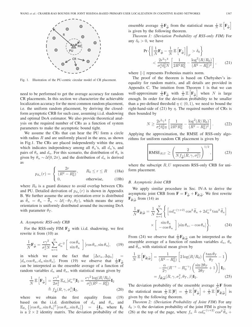
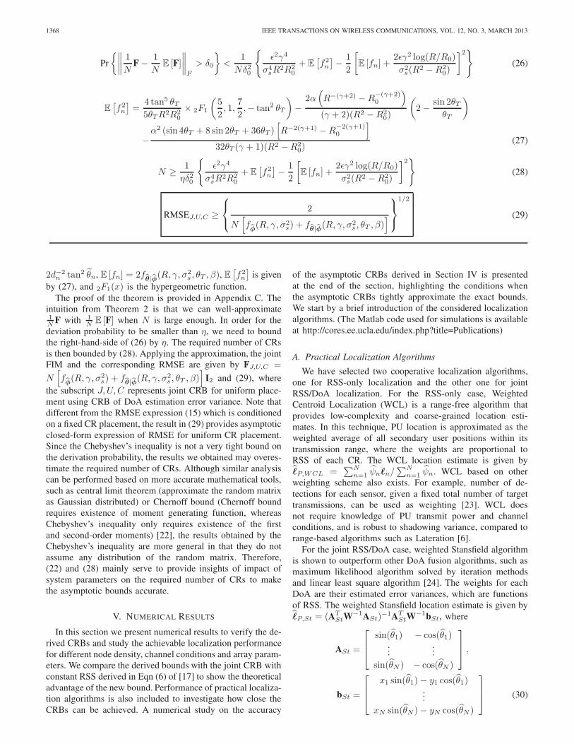
We first study the impact of node density on the localizationaccuracy. The results for the RSS-only CRB (11) and WCLalgorithm are presented in Fig.2. It is observed that addingmore CRs provides steady performance improvement for bothRSS-only CRB and WCL algorithm, and the WCL algorithmhas a constant RMSE gap of about 10m for sufficiently largenumber of CRs, say 40, compared with the RSS-only CRB.The reason for the gap is that WCL assumes no knowledge ofthe channel conditions, such as path-loss exponent, shadowingvariance and correlation distance, while the CRB uses all theabove information. The results for the derived joint CRB usingoptimal DoA estimators (15), the Stansfield algorithm withoutweighting (i.e. set the weighting matrix W in Sec. V-A toidentity matrix), and the weighted Stansfield algorithm arepresented in Fig.3. The localization accuracy of the joint CRBand the weighted Stansfield algorithm vary from 0.1 metersto 5 meters, compared with the accuracy range of 5 to 35meters for RSS-only CRB and WCL in Fig.2, and 6 to 19meters for Stansfield algorithm without weighting, indicatingthat using both RSS and DoA measurements provides muchbetter accuracy than using only RSS or DoA. The predictedaccuracy by the joint CRB is achievable by the weightedStansfield algorithm, for large number of CRs.

10 20 30 40 50 60 70 80 90 1000

5

10

15

20

25

30

35

40

Number of Nodes

RM

SE

(m

)

WCLRSS−CRB

Fig. 2. Results for RMSE of RSS-only CRB and WCL algorithm withvarying number of CRs in an uncorrelated shadowing environment (σs =6dB), with uniform random placement in a circle with R = 150m.

10 20 30 40 50 60 70 80 90 1000

2

4

6

8

10

12

14

16

18

20

Number of Nodes

RM

SE

(m

)

StanW−StanJoint−CRB

Fig. 3. Results for RMSE of the joint CRB, Stansfield algorithm andweighted Stansfield algorithm with varying number of CRs in an uncorrelatedshadowing environment (σs = 6dB), with uniform random placement in acircle with R = 150m.

D. Impact of Channel Conditions

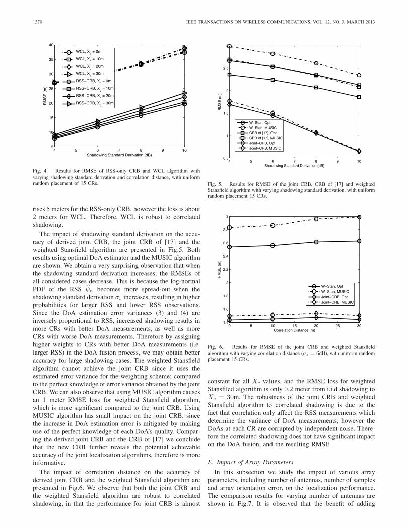
We study the impact of channel conditions including shad-owing variance and correlation distance on the localization ac-curacy. The considered values of shadowing standard deviationvary from 4 to 10dB, and the typical correlation distance formobile communication is shown to be within 30 meters [25].The results for the RSS-only CRB and the WCL algorithmsare shown in Fig.4. It is observed that increasing shadowingstandard derivation causes a linear increase in the RMSE, inthat a 2dB increase of shadowing standard derivation resultsin 4 meters accuracy loss for both RSS-only CRB and theWCL algorithm. The performance loss caused by correlatedshadowing is more significant for the RSS-only CRB thanWCL. For example, when the correlation distance increasesfrom 0 meter to 30 meters under 10dB shadowing, the RMSE


4 5 6 7 8 9 105

10

15

20

25

30

35

40

Shadowing Standard Derivation (dB)

RM

SE

(m

)

WCL, Xc = 0m

WCL, Xc = 10m

WCL, Xc = 20m

WCL, Xc = 30m

RSS−CRB, Xc = 0m

RSS−CRB, Xc = 10m

RSS−CRB, Xc = 20m

RSS−CRB, Xc = 30m

Fig. 4. Results for RMSE of RSS-only CRB and WCL algorithm withvarying shadowing standard derivation and correlation distance, with uniformrandom placement of 15 CRs.

rises 5 meters for the RSS-only CRB, however the loss is about2 meters for WCL. Therefore, WCL is robust to correlatedshadowing.

The impact of shadowing standard derivation on the accu-racy of derived joint CRB, the joint CRB of [17] and theweighted Stansfield algorithm are presented in Fig.5. Bothresults using optimal DoA estimator and the MUSIC algorithmare shown. We obtain a very surprising observation that whenthe shadowing standard derivation increases, the RMSEs ofall considered cases decrease. This is because the log-normalPDF of the RSS ψn becomes more spread-out when theshadowing standard derivation σs increases, resulting in higherprobabilities for larger RSS and lower RSS observations.Since the DoA estimation error variances (3) and (4) areinversely proportional to RSS, increased shadowing results inmore CRs with better DoA measurements, as well as moreCRs with worse DoA measurements. Therefore by assigninghigher weights to CRs with better DoA measurements (i.e.larger RSS) in the DoA fusion process, we may obtain betteraccuracy for large shadowing cases. The weighted Stansfieldalgorithm cannot achieve the joint CRB since it uses theestimated error variance for the weighting scheme; comparedto the perfect knowledge of error variance obtained by the jointCRB. We can also observe that using MUSIC algorithm causesan 1 meter RMSE loss for weighted Stansfield algorithm,which is more significant compared to the joint CRB. UsingMUSIC algorithm has small impact on the joint CRB, sincethe increase in DoA estimation error is mitigated by makinguse of the perfect knowledge of each DoA’s quality. Compar-ing the derived joint CRB and the CRB of [17] we concludethat the new CRB further reveals the potential achievableaccuracy of the joint localization algorithms, therefore is moreinformative.

The impact of correlation distance on the accuracy ofderived joint CRB and the weighted Stansfield algorithm arepresented in Fig.6. We observe that both the joint CRB andthe weighted Stansfield algorithm are robust to correlatedshadowing, in that the performance for joint CRB is almost

4 5 6 7 8 9 100.5

1

1.5

2

2.5

3

Shadowing Standard Derivation (dB)

RM

SE

(m

)

W−Stan, OptW−Stan, MUSICCRB of [17], OptCRB of [17], MUSICJoint−CRB, OptJoint−CRB, MUSIC

Fig. 5. Results for RMSE of the joint CRB, CRB of [17] and weightedStansfield algorithm with varying shadowing standard derivation, with uniformrandom placement 15 CRs.

0 5 10 15 20 25 301.4

1.6

1.8

2

2.2

2.4

2.6

2.8

3

Correlation Distance (m)

RM

SE

(m

)

W−Stan, OptW−Stan, MUSICJoint−CRB, OptJoint−CRB, MUSIC

Fig. 6. Results for RMSE of the joint CRB and weighted Stansfieldalgorithm with varying correlation distance (σs = 6dB), with uniform randomplacement 15 CRs.

constant for all Xc values, and the RMSE loss for weightedStansfiled algorithm is only 0.2 meter from i.i.d shadowing toXc = 30m. The robustness of the joint CRB and weightedStansfield algorithm to correlated shadowing is due to thefact that correlation only affect the RSS measurements whichdetermine the variance of DoA measurements; however theDoAs at each CR are corrupted by independent noise. There-fore the correlated shadowing does not have significant impacton the DoA fusion, and the resulting RMSE.

E. Impact of Array Parameters

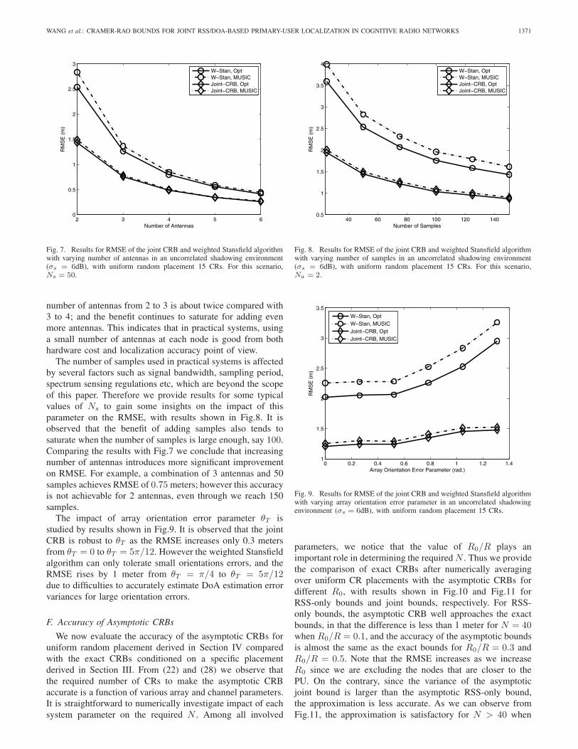
In this subsection we study the impact of various arrayparameters, including number of antennas, number of samplesand array orientation error, on the localization performance.The comparison results for varying number of antennas areshown in Fig.7. It is observed that the benefit of adding


2 3 4 5 60

0.5

1

1.5

2

2.5

3

Number of Antennas

RM

SE

(m

)


Fig. 7. Results for RMSE of the joint CRB and weighted Stansfield algorithmwith varying number of antennas in an uncorrelated shadowing environment(σs = 6dB), with uniform random placement 15 CRs. For this scenario,Ns = 50.

number of antennas from 2 to 3 is about twice compared with3 to 4; and the benefit continues to saturate for adding evenmore antennas. This indicates that in practical systems, usinga small number of antennas at each node is good from bothhardware cost and localization accuracy point of view.

The number of samples used in practical systems is affectedby several factors such as signal bandwidth, sampling period,spectrum sensing regulations etc, which are beyond the scopeof this paper. Therefore we provide results for some typicalvalues of Ns to gain some insights on the impact of thisparameter on the RMSE, with results shown in Fig.8. It isobserved that the benefit of adding samples also tends tosaturate when the number of samples is large enough, say 100.Comparing the results with Fig.7 we conclude that increasingnumber of antennas introduces more significant improvementon RMSE. For example, a combination of 3 antennas and 50samples achieves RMSE of 0.75 meters; however this accuracyis not achievable for 2 antennas, even through we reach 150samples.

The impact of array orientation error parameter θT isstudied by results shown in Fig.9. It is observed that the jointCRB is robust to θT as the RMSE increases only 0.3 metersfrom θT = 0 to θT = 5π/12. However the weighted Stansfieldalgorithm can only tolerate small orientations errors, and theRMSE rises by 1 meter from θT = π/4 to θT = 5π/12due to difficulties to accurately estimate DoA estimation errorvariances for large orientation errors.

F. Accuracy of Asymptotic CRBs

We now evaluate the accuracy of the asymptotic CRBs foruniform random placement derived in Section IV comparedwith the exact CRBs conditioned on a specific placementderived in Section III. From (22) and (28) we observe thatthe required number of CRs to make the asymptotic CRBaccurate is a function of various array and channel parameters.It is straightforward to numerically investigate impact of eachsystem parameter on the required N . Among all involved

40 60 80 100 120 1400.5

1

1.5

2

2.5

3

3.5

4

Number of Samples

RM

SE

(m

)


Fig. 8. Results for RMSE of the joint CRB and weighted Stansfield algorithmwith varying number of samples in an uncorrelated shadowing environment(σs = 6dB), with uniform random placement 15 CRs. For this scenario,Na = 2.

0 0.2 0.4 0.6 0.8 1 1.2 1.41

1.5

2

2.5

3

3.5

Array Orientation Error Parameter (rad.)

RM

SE

(m

)


Fig. 9. Results for RMSE of the joint CRB and weighted Stansfield algorithmwith varying array orientation error parameter in an uncorrelated shadowingenvironment (σs = 6dB), with uniform random placement 15 CRs.

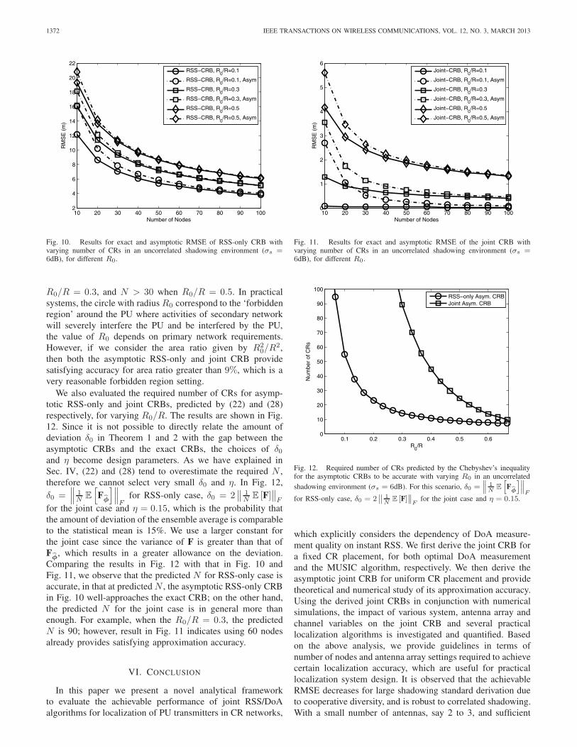
parameters, we notice that the value of R0/R plays animportant role in determining the requiredN . Thus we providethe comparison of exact CRBs after numerically averagingover uniform CR placements with the asymptotic CRBs fordifferent R0, with results shown in Fig.10 and Fig.11 forRSS-only bounds and joint bounds, respectively. For RSS-only bounds, the asymptotic CRB well approaches the exactbounds, in that the difference is less than 1 meter for N = 40when R0/R = 0.1, and the accuracy of the asymptotic boundsis almost the same as the exact bounds for R0/R = 0.3 andR0/R = 0.5. Note that the RMSE increases as we increaseR0 since we are excluding the nodes that are closer to thePU. On the contrary, since the variance of the asymptoticjoint bound is larger than the asymptotic RSS-only bound,the approximation is less accurate. As we can observe fromFig.11, the approximation is satisfactory for N > 40 when


10 20 30 40 50 60 70 80 90 1002

4

6

8

10

12

14

16

18

20

22

Number of Nodes

RM

SE

(m

)

RSS−CRB, R

0/R=0.1

RSS−CRB, R0/R=0.1, Asym

RSS−CRB, R0/R=0.3


RSS−CRB, R0/R=0.5


Fig. 10. Results for exact and asymptotic RMSE of RSS-only CRB withvarying number of CRs in an uncorrelated shadowing environment (σs =6dB), for different R0.

R0/R = 0.3, and N > 30 when R0/R = 0.5. In practicalsystems, the circle with radius R0 correspond to the ‘forbiddenregion’ around the PU where activities of secondary networkwill severely interfere the PU and be interfered by the PU,the value of R0 depends on primary network requirements.However, if we consider the area ratio given by R2

0/R2,

then both the asymptotic RSS-only and joint CRB providesatisfying accuracy for area ratio greater than 9%, which is avery reasonable forbidden region setting.

We also evaluated the required number of CRs for asymp-totic RSS-only and joint CRBs, predicted by (22) and (28)respectively, for varying R0/R. The results are shown in Fig.12. Since it is not possible to directly relate the amount ofdeviation δ0 in Theorem 1 and 2 with the gap between theasymptotic CRBs and the exact CRBs, the choices of δ0and η become design parameters. As we have explained inSec. IV, (22) and (28) tend to overestimate the required N ,therefore we cannot select very small δ0 and η. In Fig. 12,δ0 =

∥∥∥ 1N E

[Fφ

]∥∥∥F

for RSS-only case, δ0 = 2∥∥ 1N E [F]

∥∥F

for the joint case and η = 0.15, which is the probability thatthe amount of deviation of the ensemble average is comparableto the statistical mean is 15%. We use a larger constant forthe joint case since the variance of F is greater than that ofFφ, which results in a greater allowance on the deviation.

Comparing the results in Fig. 12 with that in Fig. 10 andFig. 11, we observe that the predicted N for RSS-only case isaccurate, in that at predictedN , the asymptotic RSS-only CRBin Fig. 10 well-approaches the exact CRB; on the other hand,the predicted N for the joint case is in general more thanenough. For example, when the R0/R = 0.3, the predictedN is 90; however, result in Fig. 11 indicates using 60 nodesalready provides satisfying approximation accuracy.

VI. CONCLUSION

In this paper we present a novel analytical frameworkto evaluate the achievable performance of joint RSS/DoAalgorithms for localization of PU transmitters in CR networks,

10 20 30 40 50 60 70 80 90 1000

1

2

3

4

5

6

Number of Nodes

RM

SE

(m

)

Joint−CRB, R

0/R=0.1

Joint−CRB, R0/R=0.1, Asym

Joint−CRB, R0/R=0.3


Joint−CRB, R0/R=0.5


Fig. 11. Results for exact and asymptotic RMSE of the joint CRB withvarying number of CRs in an uncorrelated shadowing environment (σs =6dB), for different R0.

0.1 0.2 0.3 0.4 0.5 0.60

10

20

30

40

50

60

70

80

90

100

R0/R

Num

ber

of C

Rs

RSS−only Asym. CRBJoint Asym. CRB

Fig. 12. Required number of CRs predicted by the Chebyshev’s inequalityfor the asymptotic CRBs to be accurate with varying R0 in an uncorrelatedshadowing environment (σs = 6dB). For this scenario, δ0 =

∥∥∥ 1N

E

[Fφ

]∥∥∥F

for RSS-only case, δ0 = 2∥∥ 1N

E [F]∥∥F

for the joint case and η = 0.15.

which explicitly considers the dependency of DoA measure-ment quality on instant RSS. We first derive the joint CRB fora fixed CR placement, for both optimal DoA measurementand the MUSIC algorithm, respectively. We then derive theasymptotic joint CRB for uniform CR placement and providetheoretical and numerical study of its approximation accuracy.Using the derived joint CRBs in conjunction with numericalsimulations, the impact of various system, antenna array andchannel variables on the joint CRB and several practicallocalization algorithms is investigated and quantified. Basedon the above analysis, we provide guidelines in terms ofnumber of nodes and antenna array settings required to achievecertain localization accuracy, which are useful for practicallocalization system design. It is observed that the achievableRMSE decreases for large shadowing standard derivation dueto cooperative diversity, and is robust to correlated shadowing.With a small number of antennas, say 2 to 3, and sufficient


∂2gn∂x2P

= − Δyn

βf(φn)d4n

{[Δxn sin(2θn) + Δyn cos(2θn)

](θn − θn)

2

+2[Δxn cos

2 θn −Δyn sin(2θn)](θn − θn)−Δyn cos

2 θn

}(34)

Eθ,φ

[∂2gn∂x2P

]= E

φ

{Eθ|φ

[∂2gn∂x2P

]}=

Δy2n cos2 θn

βd4nE

φ

[1

f(φn)

]−

Δyn

[Δxn sin(2θn) + Δyn cos(2θn)

]d4n cos

2 θn(35)

Eθ,φ

[∂2gn∂y2P

]=

Δx2n cos2 θn

βd4nE

φ

[1

f(φn)

]−

Δxn

[Δxn cos(2θn)−Δyn sin(2θn)

]d4n cos

2 θn(36)

Eθ,φ

[∂2gn

∂xP∂yP

]= −ΔxnΔyn cos

2 θnβd4n

Eφ

[1

f(φn)

]+

[ΔxnΔyn cos(2θn) +

12 (Δx

2n −Δy2n) sin(2θn)

]d4n cos

2 θn(37)

number of samples, jointly using RSS and DoA measurementsreduces the RMSE by 90% compared with using only RSS.CRB derivations for other more practical but also complexmodels of channel variation, node placement and measurementnoise [26] will be considered in our future work.

APPENDIX ADERIVATION OF F

φ AND Fθ|φ

In this appendix we provide detailed derivations to obtainelements of F

φ and Fθ|φ. For F

φ, starting from (9), eachelement in F

φ is given as{Fφ

}11

= Eφ

[∂(φ− φ)T

∂xPΩ−1

s∂(φ− φ)

∂xP

+(φ− φ)Ω−1s∂2(φ− φ)

∂x2P

](31)

{Fφ

}22

= Eφ

[∂(φ− φ)T

∂yPΩ−1

s∂(φ− φ)

∂yP

+(φ− φ)Ω−1s∂2(φ− φ)

∂y2P

](32)

{Fφ

}12

= Eφ

[∂(φ− φ)T

∂xPΩ−1

s∂(φ− φ)

∂yP

+(φ− φ)Ω−1s∂2(φ− φ)

∂xP∂yP

](33)

and{

Fφ

}21

={

Fφ

}12

, where elements for all vectors of

derivatives are given by ∂(φn−φn)∂xP

= 10γlog 10

Δxn

d2n, ∂(

φn−φn)∂yP

=

10γlog 10

Δynd2n

, ∂2(φn−φn)∂x2

P= 10γ

log 10Δy2n−Δx2

n

d4n, ∂2(φn−φn)

∂y2P=

10γlog 10

Δx2n−Δy2nd4n

, ∂2(φn−φn)∂xP ∂xP

= − 20γlog 10

ΔxnΔynd4n

. Applying theexpectation in (31-33) with the derivatives results in (10).

For Fθ|φ, starting from (13), the second order derivatives of

gn over xP is given by (34) at the top of the page. Note thathere we use the general form f(φn) to represent the functionof RSS in the DoA estimation error variance, instead of usingspecific functions such as fCRB(φn) or fMU (φn). Thereforethe results in this appendix can be applied to derivation of F

θ|φ

of both assuming optimal DoA estimation or using MUSICalgorithm. When we take expectations of (34), we apply thefollowing property of taking expectation of a function f(x, y)of two random variables X and Y with known joint PDFp(x, y): EX,Y [f(x, y)] = EY

{EX|Y [f(x, y)]

}, and get (35).

Applying similar procedure to ∂2gn∂xP ∂yP

and ∂2gn∂y2P

, we obtain

(36) and (37). Now we consider different f(φn) given byCRB or MUSIC, which results in (38a) and (38b) at thetop of the next page, where the expectation in (38b) is anexpectation of inverse of shifted log-normal variable, whichis not directly obtainable and need to be calculated throughnumerical methods.

The expectations of second order derivatives of hn over thePU coordinates are given by

Eθ,φ

[∂2hn∂x2P

]= − Δyn

d4n cos2 θn

[Δyn +Δxn sin(2θn)

]Eθ,φ

[∂2hn∂y2P

]= − Δxn

d4n cos2 θn

[Δxn −Δyn sin(2θn)

]Eθ,φ

[∂2hn

∂xP∂yP

]=

1

d4n cos2 θn

[ΔxnΔyn

+1

2(Δx2n −Δy2n) sin(2θn)

]. (39)

Summation of corresponding elements in (35), (36), (37) and(39) with some simplification will give us the elements ofsub-FIM F

θ|φ.

APPENDIX BDERIVATION OF THE DISTRIBUTION OF dn

In this appendix we derive the distribution of dn for uniformrandom CR placement in the ring-area specified by radius R0

and R. In such case, the CR coordinates �n = [xn, yn]T has

the following PDF fxn,yn(x, y)

fxn,yn(x, y) =

⎧⎨⎩1

π(R2 −R20), R2

0 ≤ x2 + y2 ≤ R2(40a)

0, otherwise. (40b)

The relationship between fxn,yn(x, y) and fdn,θn(r, θ), thePDF of dn and θn, is given by fxn,yn(x, y)dxdy =


Eφ

[1

f(φn)

]=

⎧⎪⎪⎪⎨⎪⎪⎪⎩c0PT e

σ2s/(2ε)

dγn, CRB, (38a)

c0PT eσ2s/(2ε)

dγn− PMNa

+P 2M

N2a

Eφ

[1

ψn + PM

Na

], MUSIC, (38b)

fdn,θn(r, θ)drdθ. Therefore we have

fdn,θn(r, θ) = fxn,yn(x, y)

∣∣∣∣dxdydrdθ

∣∣∣∣ = fxn,yn(x, y)

∣∣∣∣∂(x, y)∂(r, θ)

∣∣∣∣= fxn,yn(x, y)r, (41)

where |·| denotes matrix determinant and the third equalityis obtained by the transformations xn = dn cos θn and yn =dn sin θn (i.e. x = r cos θ and y = r sin θ). Given that θn ∼U(0, 2π) and it is independent to dn, Substituting (40a) and(40b) into (41) and some simple manipulations generate (18a)and (18b).

APPENDIX CPROOF OF THEOREM 1 AND 2

We start by introducing the Chebyshev’s inequality forrandom matrix, which will be the tool for the following proof.

Theorem 3: (Chebyshev’s Inequality for Random Matrix)Suppose X is a random matrix with mean E [X] and its secondorder moments exist. Then for any δ > 0, we have

Pr {‖X − E [X]‖ > δ} <E

[‖X − E [X]‖2

]δ2

, (42)

where ‖·‖ denotes any matrix norm.Proof: From the Markov’s inequality which states that

if X is a nonnegative random variable, and E [X ] is itsmean, then for any δ > 0, we have Pr{X > δ} < E[X]

δ .Therefore, for scalar random variable ‖X − E [X]‖2, we have

Pr{‖X − E [X]‖2 > δ2

}<

E[‖X−E[X]‖2]δ2 . Taking square root

of the expression on the left-hand-side finishes the proof.To prove Theorem 1, we observe from the Chebyshev’s

inequality that we need to compute E

[‖X − E [X]‖2F

]for

X = 1N F

φ, where the Frobenius norm is given by ‖ X ‖F=√Tr(XTX). As a result, we need to evaluate the following

expression

E

{Tr

[(1

NFφ − 1

NE

[Fφ

])T (1

NFφ − 1

NE

[Fφ

])]}

=1

N2Tr

{E

[(Fφ − E

[Fφ

])T (Fφ − E

[Fφ

])]}.(43)

The covariance of Fφ appeared in the right-hand-side of (43)

can be derived from (19) as

E

[(Fφ − E

[Fφ

])T (Fφ − E

[Fφ

])]=ε2γ4N

σ4s

[1

2R2R20

− log2(R/R0)

(R2 −R20)

2

]I2. (44)

From (43) and (44) we obtain that

E

[∥∥∥∥ 1

NF

φ − 1

NE

[F

φ

]∥∥∥∥2

F

]=

2ε2γ4

σ4sN

[1

2R2R20

− log2(R/R0)

(R2 −R20)

2

].

(45)

The application of Theorem 3 on∥∥∥ 1N F

φ − 1N E

[Fφ

]∥∥∥F

withresult of (45) proves Theorem 1.

To prove Theorem 2, we observe from the Chebyshev’sinequality that we need to compute E

[‖X − E [X]‖2F

]for X =

1N F, which requires evaluation of the following expression

E

{Tr

[(1

NF − 1

NE [F]

)T (1

NF − 1

NE [F]

)]}=

1

N2Tr

{E

[(F − E [F])T (F − E [F])

]}. (46)

The covariance of F = Fφ + F

θ|φ appeared on the right-hand-side of (46) can be derived as (47) at the top of thepage, where fn, E [fn] and E

[f2n

]are defined in Theorem 2.

We skip the derivations to obtain (47) which include tediousmanipulations of (19) and (24). From (46) and (47) we obtain(48). The application of Theorem 3 on

∥∥ 1N F − 1

N E [F]∥∥F

with result of (48) proves Theorem 2.

REFERENCES

[1] J. Mitola and G. Maguire, “Cognitive radio: making software radiosmore personal,” IEEE Personal Commun., vol. 6, no. 4, pp. 13–18, Aug.1999.

[2] S. Haykin, “Cognitive radio: brain-empowered wireless communica-tions,” IEEE J. Sel. Areas Commun., vol. 23, no. 2, pp. 201–220, Feb.2005.

[3] H. Celebi and H. Arslan, “Utilization of location information in cogni-tive wireless networks,” IEEE Wireless Commun. Mag., vol. 14, no. 4,pp. 6–13, Aug. 2007.

[4] N. Patwari, J. Ash, S. Kyperountas, A. Hero, R. Moses, and N. Cor-real, “Locating the nodes: cooperative localization in wireless sensornetworks,” IEEE Signal Process. Mag., vol. 22, no. 4, pp. 54–69, July2005.

[5] E. Kaplan and C. Hegarty, Understanding GPS: Principles and Appli-cations. Artech House, 2005.

[6] J. Wang, P. Urriza, Y. Han, and D. Cabric, “Weighted centroid local-ization algorithm: theoretical analysis and distributed implementation,”IEEE Trans. Wireless Commun., vol. 10, no. 10, pp. 3403–3413, Oct.2011.

[7] M. Gavish and A. Weiss, “Performance analysis of bearing-only targetlocation algorithms,” IEEE Trans. Aerosp. Electron. Syst., vol. 28, no. 3,pp. 817–828, July 1992.

[8] R. Stansfield, “Statistical theory of d.f. fixing,” J. Inst. Electr. Eng.,vol. 94, no. 15, pp. 762–770, Mar. 1947.

[9] P. Stoica and N. Arye, “Music, maximum likelihood, and Cramer-Raobound,” IEEE Trans. Acoust., Speech, Signal Process., vol. 37, no. 5,pp. 720–741, May 1989.

[10] V. Savic, A. Athalye, M. Bolic, and P. Djuric, “Particle filtering forindoor RFID tag tracking,” in Proc. 2011 IEEE Statistical SignalProcess. Workshop, pp. 193–196.

[11] N. Patwari and P. Agrawal, “Effects of correlated shadowing: connectiv-ity, localization, and RF tomography,” in Proc. 2008 ACM/IEEE IPSN,pp. 82–93.


E

[(F − E [F])T (F − E [F])

]= N

{ε2γ4

2σ4sR

2R20

+1

2E[f2n

]− 1

4

[E [fn] +

2εγ2 log(R/R0)

σ2s (R

2 −R20)

]2 }I2, (47)

E

[∥∥∥∥ 1

NF − 1

NE [F]

∥∥∥∥2

F

]=

1

N

{ε2γ4

σ4sR

2R20

+ E[f2n

]− 1

2

[E [fn] +

2εγ2 log(R/R0)

σ2s (R

2 −R20)

]2}. (48)

[12] F. Gustafsson and F. Gunnarsson, “Mobile positioning using wirelessnetworks: possibilities and fundamental limitations based on availablewireless network measurements,” IEEE Signal Process. Mag., vol. 22,no. 4, pp. 41–53, July 2005.

[13] J. Ash and R. Moses, “On the relative and absolute positioning errors inself-localization systems,” IEEE Trans. Signal Process., vol. 56, no. 11,pp. 5668–5679, Nov. 2008.

[14] C. Seow and S. Tan, “Non-line-of-sight localization in multipath envi-ronments,” IEEE Trans. Mobile Comput., vol. 7, no. 5, pp. 647–660,May 2008.

[15] R. Vaghefi, M. Gholami, and E. Strom, “Bearing-only target localizationwith uncertainties in observer position,” in Proc. 2010 IEEE PIMRC,pp. 238–242.

[16] Y. Fu and Z. Tian, “Cramer-Rao bounds for hybrid TOA/DOA-basedlocation estimation in sensor networks,” IEEE Signal Process. Lett.,vol. 16, no. 8, pp. 655–658, Aug. 2009.

[17] F. Penna and D. Cabric, “Bounds and tradeoffs for cooperative DOA-only localization of primary users,” in Proc. 2011 IEEE GLOBECOM,pp. 1–5.

[18] Y. Qi, H. Kobayashi, and H. Suda, “Analysis of wireless geolocation in anon-line-of-sight environment,” IEEE Trans. Wireless Commun., vol. 5,no. 3, pp. 672–681, Mar. 2006.

[19] R. Schmidt, “Multiple emitter location and signal parameter estimation,”IEEE Trans. Antennas Propag., vol. 34, no. 3, pp. 276–280, Mar. 1986.

[20] R. Roy and T. Kailath, “Esprit-estimation of signal parameters viarotational invariance techniques,” IEEE Trans. Acoust., Speech, SignalProcess., vol. 37, no. 7, pp. 984–995, July 1989.

[21] Y. Shen and M. Win, “On the accuracy of localization systems usingwideband antenna arrays,” IEEE Trans. Commun., vol. 58, no. 1, pp.270–280, Jan. 2010.

[22] J. G. Proakis, Digital Communications. McGraw-Hill, 2001.[23] A. Athalye, V. Savic, M. Bolic, and P. Djuric, “A radio frequency

identification system for accurate indoor localization,” in Proc. 2011IEEE ICASSP, pp. 1777–1780.

[24] J. Wang and D. Cabric, “A cooperative DOA-based algorithm forlocalization of multiple primary-users in cognitive radio networks,” inProc. 2012 IEEE GLOBECOM.

[25] P. Taaghol and R. Tafazolli, “Correlation model for shadow fading inland-mobile satellite systems,” Electron. Lett., vol. 33, no. 15, pp. 1287–1289, July 1997.

[26] C. Whitehouse, “Understanding the prediction gap in multi-hop local-ization,” Ph.D. thesis, 2006.

Jun Wang (S’09) received his B.E. degree in Elec-tronic Information Engineering from Beijing Univer-sity of Technology and MPhil degree in ElectricalEngineering from City University of Hong Kong, in2006 and 2009, respectively. In 2009, he joined theElectrical Engineering Department of the Universityof California Los Angeles as a Ph.D. student, ad-vised by Prof. Danijela Cabric. His research interestincludes acquisition and utilization of primary-userlocation information and various issues related tospectrum sensing in cognitive radio networks.

Jianshu Chen (S’10) received his B.S. and M.S.degrees in Electronic Engineering from Harbin In-stitute of Technology in 2005 and Tsinghua Uni-versity in 2009, respectively. He is currently work-ing towards the Ph.D. degree in the Departmentof Electrical Engineering, University of California,Los Angeles (UCLA). Since 2009, he has been amember of the Adaptive Systems Laboratory (ASL)at UCLA. His research interests include statisticalsignal processing, adaptive networks, and distributedoptimization.

Danijela Cabric received the Dipl. Ing. degree fromthe University of Belgrade, Serbia, in 1998, andthe M.Sc. degree in electrical engineering from theUniversity of California, Los Angeles, in 2001. Shereceived her Ph.D. degree in electrical engineer-ing from the University of California, Berkeley, in2007, where she was a member of the BerkeleyWireless Research Center. In 2008, she joined thefaculty of the Electrical Engineering Departmentat the University of California, Los Angeles as anAssistant Professor. Her research interests include

novel radio architecture, signal processing, and networking techniques toimplement spectrum sensing functionality in cognitive radios. Dr. Cabricreceived the Samueli Fellowship in 2008, the Okawa Foundation ResearchGrant in 2009, and the National Science Foundation Faculty Early CareerDevelopment Award in 2012.

Documents

Cramer-Rao Bounds for Joint RSS/DoA-Based Primary-User Localization in Cognitive Radio Networks