Embed Size (px)
Citation preview

NASA CR-137,917
APPLICATION OF THE ADAPTIVE-WALL CONCEPT
TO THREE-DIMENSIONAL LOW-SPEED WIND TUNNELS
By J.. C. Erickson, Jr.
September 1976
Distribution of this report is provided in the interest of information ,exchange. Responsibility for the contents resides
in the author or organization that prepared it.
I(NASA-CR-137917) APPLICATION OF THE N76-32200 ADAPTIVE-WALL CONCEPT TO THREE-DIMENSIONAL LOU-SPEED WIND TUNNELS (Calspan Corp.,iBuffalo, N.Y.) 77 p HC $5.00 CSCL 14B
-3/09 Unclas 01589.
Prepared under Contract No. NAS2-8777 by Calspan Corporation Buffalo, New York
for
AMES RESEARCH CENTER
NATIONAL AERONAUTICS AND SPACE ADMINISTRATION
rIO 7-7 t\
https://ntrs.nasa.gov/search.jsp?R=19760025112 2018-06-29T18:56:38+00:00Z

1.Report No. 2. Government Accssiorn No. 3. Retipent's Catatog No.
NASA CR-137 917 4. Title and Subtitle 5.Report DateSeptember 1976
Application of the Adaptive-Wall Concept to 6.Performing Organization Code
Three-Dimensional Low-Speed Wind Tunnels
7. Author(s) 8. Performing Organization Report No.
J.C. Erickson, Jr. RK-5717-A-1 10. Work Unit No.
9. Performing Organization Name and Address
Calspan Corporation 11. Contract or Grant No.
P.O. Box 235 NAS2-8777 Buffalo, New York 14221 13. T}pu of Fe-rq and Period co:ered
12. Sponsoring Agency Name and Addrtss Contractor Report National Aeronautics and Space Administration1 Cod...
por.,,i, Aency CodeAmes Research Center S14.
Moffett Field, California 94035 15. SpLmmntary Notes
16. Absttact
Interference-free flows about a'model in a wind tunnel exist when certain functional relationships are satisfied among disturbance velocity components at a measurement control surface located within the tunnel near, or at, the walls. These functional relationships are derived for three-dimensional subcritical 'flow fields in which no propulsion-system efflux intersects the control surface !until far downstream. Three methods for evaluating the functional relationships have been developed. The first of these, the original multipole expansion (MPE) procedure, is based on a series of point singularities which satisfy the governing Prandtl-Glauert equation. The second, the modified MPE, provides an improved representation of finite-span wings and thereby extends the range of validity of the original MPE to larger ratios of span-to-control-surface-width. The third method is more general and is based on source distributions over the control surface.. Several numerical examples are presented to help establish the range of validity of these evaluation methods. An accuracy-assessment procedure, which combines the original MPE procedure with classical wall-correction theory, has been developed to estimate the degree of interference at the model if the functional relationships are not satisfied exactly. Several numerical examples of this procedure are presented for representative wings and bodies.
.7. Key Words (Suggested by Author(s)) 18. Distribution Statement
Self-Correcting Wind Tunnels Adaptive-Wall Wind Tunnels V/STOL Wind Tunnels Wind Tunnel Wall Interference
19. Sxurity Ocs'if. (of this reportl 20. Sccurity Classif. (of tis page) 21. No. of Pao-= 22. Price'
Unclassified Unclassified 75
For zieby the N.tionafTechnical Int' ct Ss-vice, Splna.",z:J, V:rsi-.a 22151
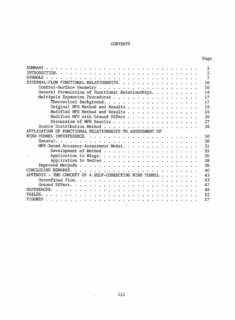
CONTENTS
Page
SUMMARY ."....................... ......... 1 INTRODUCTION................ ........................... 2 SYMBOLS ................. ............................ 7 EXTERNAL-FLOW FUNCTIONAL RELATIONSHIPS. . ........... ......... 10
Control-Surface Geometry .......... ..................... 10 General Formulation of Functional Relationships... . ...... 14 Multipole Expansion Procedures ...... ........... ...... 17
Theoretical Background....... .................... ... 17 Original MPE Method and Results ..... ............... ... 19 Modified MPE Method and Results ..... ............... ... 24 Modified MPE with Ground Effect .... ........... ..... 26 Discussion of MPE Results ...... ................. .... 27
Source Distribution Method ....... .................... ... 28 APPLICATION OF FUNCTIONAL RELATIONSHIPS TO ASSESSMENT OF WIND-TUNNEL INTERFERENCE.......... ..................... ... 30
General............ .............................. . 30 MPE-Based Accuracy-Assessment Model.... ........ . .. ...... 31
Development of Method ....... .................... ... 31 Application to Wings.... ......................... 35 Application to Bodies ........ . ................... 38
Improved Methods ...... ......................... .. 39 CONCLUDING REMARKS .......... .......................... .... 40 APPENDIX - THE CONCEPT OF A SELF-CORRECTING WIND TUNNEL ............. 43
Unconfined Flow.......... .......................... ... 43 Ground Effect.......... ...................... ..... 47
REFERENCES................ ................ .......... 48 TABLES............. ................................. ... 52 FIGURES ............. ...................... ......... 57
iii
APPLICATION OF THE ADAPTIVE-WALL CONCEPT
TO THREE-DIMENSIONAL LOW-SPEED WIND TUNNELS
By J. C. Erickson, Jr. Calspan Corporation
SUMMARY
Interference-free flows about a model in a wind tunnel exist when certain
functional relationships are satisfied among disturbance velocity components at a measurement control surface located within the tunnel near, or at, the walls.
These functional relationships are derived for three-dimensional subcritical flow fields in which no propulsion-system efflux intersects the control surface until far downstream. Three methods for evaluating the functional relation
ships have been developed. The first of these, the original multipole expansion (MPE) procedure, is based on a series of point singularities which satisfy the governing Prandtl-Glauert equation. The second, the modified MPE, provides
an improved representation of finite-span wings and thereby extends the range of validity of the original MPE to larger ratios of span-to-control-surface
width. The third method is'more general and is based on source distributions
over the control surface. Several numerical examples are presented to help establish the range of validity of these evaluation methods.
An accuracy-assessment procedure, which combines the original MPH pro
cedure with classical wall-correction theory, has been developed to estimate
the degree of interference at the model if the functional relationships are not satisfied exactly. Several numerical examples of this procedure are pre
*ented for representative wings and bodies.
INTRODUCTION
The flow fields about helicopters and other V/STOL aircraft are highly
complex and are difficult both to simulate in a wind tunnel and to predict
analytically. Many V/STOL designs incorporate integrated lift and propulsion
systems that are characterized by a high-energy efflux which is deflected
downward at a large angle to the direction of flight in order to generate lift
at low flight speeds. Flight speeds of these vehicles range from hover, or
near hover, through transition to cruise flight, so that the disturbance
velocities introduced by the yehicles, including their propulsion systems, are
comparable to, or even greater than, the flight velocity over an important
operating range. Thus, in wind-tunnel testing of V/STOL aircraft, the
presence of the tunnel boundaries causes larger interference effects than
exist for comparably-sized conventional aircraft with their relatively smaller
flow disturbance velocities. The necessity for large wind-tunnel models is
indicated to minimize scaling effects, which are not well understood, and to
facilitate modeling the propulsion systems, especially those with high disk
loadings such as fans and jets. These considerations, in part, have led to
the requirements for even larger testing facilities (ref. 1).
The concept of wind-tunnel-boundary corrections in solid-wall and open
jet tunnels for conventional aircraft configurations in subsonic, subcritical
flight generally has proved adequate. This results principally because the
aircraft generates only small disturbances in the flow, including a trailing
vortex system due to lift which does-not deflect significantly from the direction
of flight. These vehicles and the wall boundary conditions then can be repre
sented analytically by linearized aerodynamic theory with all its powerful
techniques and connotations, e.g., superposition. Therefore, boundary-induced
corrections to the incident flow can be interpreted in terms of corrections to
the measured aerodynamic characteristics of the vehicle, making use of the
extensive knowledge of the general aerodynamic behavior of this class of con-
The idea of corrections becomes less viable for conventionalfigurations.
aircraft configurations in ventilated tunnels, especially as the flight speed
2

becomes transonic with larger flow disturbances, loss of superposition, un
certainty in the form of the wall boundary conditions, and flow fields that
cannot be predicted accurately.
The concept of tunnel-boundary corrections for helicopters and V/STOL
aircraft also rests on a less than satisfactory basis. The propulsion-system
efflux often interacts strongly with the rest of the aircraft and generates a
highly-deflected trailing-vortex system which may also interact with the tunnel
boundaries. Also, as mentioned above, the flow disturbance velocities intro
duced by the vehicle may be comparable to, or greater than, the flight velocity
at low speeds near hover and during transition. Therefore, these vehicles
cannot be represented adequately by linearized aerodynamic models and so
superposition is no longer valid. As a result, the unconfined-flow aerodynamic
characteristics are not well understood and cannot be predicted as well as for
conventional aircraft. Therefore, even if tunnel-boundary-induced velocity
disturbances to the incident flow can be estimated accurately, their inter
pretation in terms of the measured aerodynamic characteristics may not be
possible. Finally, the basic nature of the flow in the tunnel may bear no
relationship whatsoever to the flow field in free flight, as shown first by
Rae (ref. 2). That is, there may be a flow breakdown consisting of a recir
culation of the propulsion-system efflux upstream and around the tunnel walls.
Flow breakdown occurs in a given tunnel, for a given vehicle configuration,
below some minimum tunnel speed (refs. 2-8). In view of these considerations,
tunnel-boundary effects and corrections for them are not in a fully satis
factory state for helicopter and V/STOL testing.
The difficulties in wind-tunnel testing of V/STOL configurations have
motivated considerable research in recent years. These efforts have followed
three rather broad lines. First has been the development of theoretical
methods for calculating boundary-induced interference-velocity distributions
within the test section. These methods are in the spirit of classical tunnel
boundary-correction theory and are based on simplified analytical representa
tions of various tunnel-wall and vehicle configurations including the propulsion
system efflux. Some of the principal contributions to this line of development
3

have been by Heyson (refs. 9-12), Lo, Binion and Kraft (refs. 13-17), and
Joppa (ref. 18). Second are the experimental investigations which have examined
the nature of the interference on representative models and on the nature of
the flow within the test section. These investigations (refs. 2-8) discovered
the existence of flow breakdown and have examined the conditions for its
occurrence. Finally, the third area of research on tunnel-boundary effects is
an outgrowth of the theoretical calculation of interference-velocity distri
butions. This research is aimed at the development of test-section geometrical
configurations which minimize the interference velocities and/or make them
more nearly uniform over the complete extent of typical models, so that cor
rections can be made for any residual wall effects .(refs. 13-15, 19-20). The
validity of these test-section configurations relies on the ability to repre
sent analytically the vehicle, its propulsion system, and the characteristics
of flow through ventilated walls. Consequently, the results of these studies
serve principally as guides to the objective of low-interference tunnels.
Thus, they have been augmented by experimental investigations with similar
objectives (refs. 21-28). Notable among these latter investigations are those
of Kroeger and Martin (refs. 21-22) and of Bernstein and Joppa (refs. 27-28)
because they introduce active control of the flow in the tunnel by applying
blowing and suction through ventilated tunnel walls. Their wall-control
requirements are determined from computations of the flow field near the walls
by means of a theoretical representation of the geometrical configuration to
be tested. Therefore, their method can be only as good as their ability to
predict this model flow field accurately. Hence, for complicated V/STOL
models over a large portion of their flight envelope, this can be an important
limitation.
The approaches just described hold promise for developing V/STOL test
section configuratiQns with low levels of boundary interference. Nevertheless,
each tunnel design is tied closely to a specific vehicle configuration and
size, so that generalization is difficult. Even more important, there is no
way, other than to test the same model in a larger (and therefore, supposedly
interference-free) tunnel, to verify that the boundary interference actually
has been eliminated. A further, -and significant, conceptual step which removes
4

some of these restrictions is the self-correcting, or adaptive-wall, wind
tunnel proposed by Sears Cref. 29). The self-correcting tunnel concept, which
is described more fully in the Appendix, also uses active control of the flow
at the tunnel walls. In addition, however, measurements of flow disturbance
quantities at a suitable control surface within the tunnel are combined, in
iterative fashion, with the evaluation of appropriate functional relation
ships. Satisfaction of the functional relationships by the measured flow
disturbance quantities assures that the flow about the model is interference
free.
Application of the adaptive-wall concept to transonic wind tunnels is
being pursued actively by several groups at this time, see references 29 to 36.
In particular, an experimental demonstration of the fully implemented concept,
as applied to a two-dimensional transonic tunnel, is being carried out in the
Calspan One-Foot Wind Tunnel. In this tunnel, active wall control is achieved
by segmenting the plenum surrounding the porous walls, and controlling the flow
through the walls by applying suction or pressure to the plenum segments.
Important progress to date on this work is reported in references 29 to 31.
For low speeds as well, the ultimate embodiment of the adaptive-wall
concept would have the capability to guarantee an interference-free flow in
the test section for any V/STOL configuration and attitude with respect to the
free stream. Thus, the concept incorporates the following considerations.
Unconfined flow about an arbitrary V/STOL configuration certainly cannot be
calculated with sufficient accuracy that wind-tunnel testing can be eliminated.
On the other hand, the boundaries of a wind tunnel can cause so much inter
ference with the flow about a model that the test results may be in question,
especially at very low free-stream speeds. Although the flow field in the
vicinity of the model cannot be predicted analytically, the flow field ex
ternal to the control surface is represented by a well-posed boundary-value
problem that is within the capability of existing analytical and computational
techniques. Therefore, by combining theory and experiment in a way that uses
each to its best advantage, the self-correcting wind tunnel offers the prospect
of simulation of free-flight conditions in the flow about the model.
5

The adaptive-wall wind tunnel concept can also be applied to testing in
existing conventional tunnels without provisions for flow control by the
walls. In this application, measurements still would be made at a suitable
control surface in the tunnel, and the unconfined-flow functional relation
ships would be evaluated for each test, just as described. If the functional
relationships were found to be satisfied to within some specified accuracy,
the test could be considered effectively unconfined by the walls so that the
data could be considered interference free. If, on the other hand, the
functional relationships were not satisfied to the specified accuracy, the
data would contain interference effects. Carrying this idea a step further,
the self-correcting concept could even provide a basis for improved techniques
for computing wall-interference corrections, when such corrections are meaningful.
We thus see that by means of measurements and evaluations of functional
relationships, the basic self-correcting tunnel concept can be used to establish
criteria for the accuracy of tests without wall control. Irrespective of
which mode of operation is selected, i.e., elimination of interference or
evaluation of the degree of interference present, many of the theoretical and
measurement techniques which must be investigated are identical. Therefore,
the initial research reported here is applicable either to the development of
a complete self-correcting V/STOL tunnel or to the use of measurements and
functional relationships as an indication of interference-free conditions in
existing tunnels.
In the next section, the functional relationships that must be satisfied
in wall-interference-free flow are established for conventional three-dimensional
models, for which no propulsion-system efflux intersects the measurement control
surface until far downstream. Evaluation of the functional relationships for
conventional models by means of two techniques, namely multipole expansion
(MPE) procedures and a source distribution method, are described along with
typical results for models both in and out of ground effect. The question of
assessing the accuracy required in satisfying the unconfined-flow functional
relationships, as far as the interference on the wind-tunnel model is concerned,
is discussed in the following section. A procedure for such an accuracy
6

assessment is developed using conventional tunnel-interference theory together with flow measurements and use of the MPE technique for evaluating the
functional relationships. Several examples are given which show permissible amounts of departure from the exact evaluation of the functional relationships. Finally, conclusions are given for this first step in the investigation of the
self-correcting wind tunnel concept for V/STOL testing.
SYMBOLS
/R aspect ratio, 4b. /451
a half-width of control surface (see figure 1)
b half-height of control surface (see figure 1)
bb half-length of body
bh semispan of horseshoe vortex in modified multipole expansion
b, semispan of wing
Co drag coefficient, Fo/!
CL lift coefficient, F/,4
C0 pressure coefficient, -p/&
C1 source strength in accuracy-assessment method (see equation (47))
C2 infinitesimal-span horseshoe vortex strength in accuracy-assessment
method (see equation (48))
C3 doublet strength in accuracy-assessment method (see equation (49))
wing chord in two-dimensional- flow (see figure 16)
D function defined in Table I
F drag force
FL lift force
c
7

3 functions defined in Table I
- control-surface location in two-dimensional flow (see figure 16)
1,4",hI
height of model above ground (see figures 12 and 13)
J number of terms in multipole expansion
H,. freestream Mach number
Ni coefficient of I term in multipole expansion of v,. (see equation (31))
n coordinate normal to control surface (see figure 1)
p static pressure disturbance
9 freestream dynamic pressure, /Ow ,0 /2
distance from origin to point on control-surface cross section
(see figure 1)
R function defined in Table I
r distance from control surface to field point (see equation (23))
g control surface at which flow disturbance measurements are made
(see figures 1, 15 and 16)
5 -reference area of model
T function of diameter-to-length ratio of Rankine solid, given
T = T (+T- T) ' implicitly by
t coordinate tangential to control surface (see figure 1)
UI freestream velocity
normal, tangential components of velocity induced by $h multipole
singularity of unit strength (see equations (39) and (40))
J X, V, j components of velocity induced by j multipole singularity
of unit strength (see Table I)
V model volume
t;,,7v4 normal, tangential components of disturbance velocity
zr,,v~ z, , components of disturbance velocity
8

X coefficient of ith term in multipole expansion of zrz -" (see equation (28))
xq, basic coordinate system (see figure 1)
X, offset of center of model from origin
Y, coordinate of control-surface cross section
q~ functions defined in Table I
a_ model angle of attack
a effective model angle of attack due to parabolic-arc camber
fT, of horseshoe vortex in modified multipole expansion-strength
(see equation (41))
A( ),Aiwall-interference correction to quantity ( ) based on V.. boundary conditions
i9 polar angle of point on control-surface cross section (see figure l)
9 eccentric angle of point on elliptical control-surface cross
section (see equation (7))
&c polar angle of corner of rectangular control-surface cross section
(see equation (9))
4 freestream density
0 strength of source distribution on control surface
V diameter-to-length ratio of Rankine solid
acceleration potential
S disturbance velocity potential
idealized disturbance velocity potential of model in unconfined flow
4' interference disturbance velocity potential induced by tunnel boundaries
angle between n and axes for control surface (see figure 1)
9

c
Subscripts:
calculated by evaluation of functional relationships
II index of term in multipole expansion
Mt measured at control surface
w0 free stream
EXTERNAL-FLOW FUNCTIONAL RELATIONSHIPS
Control-Surface Geometry
The functional relationships which must be satisfied among the measured
flow disturbance quantities in order for unconfined-flow conditions to exist
-in a flow will be discussed with respect to figure 1. This figure describes
a flow with free stream speed U. in the --direction about a body located
near the origin of a rectangular Z , , coordinate system. We are con
cerned principally with the flow field external to the control surface S which
encldses the body. Only part of the control surface is shown in figure 1
because it is assumed to extend infinitely far upstream and downstream with a
uniform cross section. The question of the effect of truncating the control
surface to a finite length is an important one, which must be considered
ultimately. Answering this question requires a more detailed consideration of
the flow field within the tunnel than has'been considered here.
We assume that the cross section of the control surface can be expressed
= parametrically in terms of the angle & by v YCO) and 3 = z () '. The
angle C is measured conveniently from the, -axis, as shown in figure 1,
because the Z- plane is the plane of symmetry for most'aircraft configura
tions in longitudinal flight. We assume further that the control surface is
symmetrical about the Z-; and Z-V planes with width 2a and height 2b as
shown. The coordinate t tangent to the control surface is a curvilinear
10
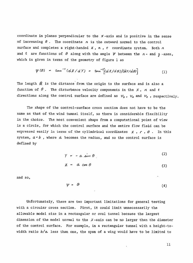
coordinate in planes perpendicular to the Z-axis and is positive in the sense
of increasing B . The coordinate n is the outward normal to the control
surface and completes a right-handed Z , n , t coordinate system. Both a
and t are functions of 0 along with the angle V between the n- and . -axes,
which is given in terms of the geometry of figure 1 as
3lrW) = o-' (~Ldcy) = o.-'cd/d)CcLy/da] (1)
The length 02 is the distance from the origin to the surface and is also a
function of 0 . The disturbance velocity components in the X, a and t
directions along the control surface are defined as 24, v and 4t , respectively.
The shape of the control-surface cross section does not have to be the
same as that of the wind tunnel itself, so there is considerable flexibility
in the choice. The most convenient shape from a computational point of view
is a circle, for which the control surface and the entire flow field can be
expressed easily in terms of the cylindrical coordinates Z , r , 0 . In this
system, a =b , where a becomes the radius, and so the control surface is
defined by
Y = -(2)
Z 0- 0coo (3)
and so,
?'V 98(4)
Unfortunately, there are two important limitations for general testing
with a circular cross section. First, it could limit unnecessarily the
allowable model size in a rectangular or oval tunnel because the largest
dimension of the model normal to the x-axis can be no larger than the diameter
of the control surface. For example, in a rectangular tunnel with a height-to
width ratio b/. less than one, the span of a wing would have to be limited to
11
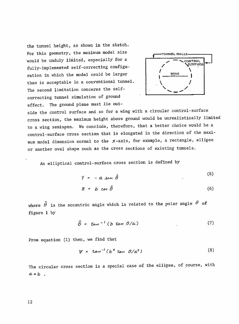
the tunnel height, as shown in the sketch.
--TUNNELWALLSFor this geometry, the maximum model size
would be unduly limited, especially for a r -CONTROL
/ \atgrcEfully-implemented self-correcting configu-__WINGration in which the model could be larger
than is acceptable in a conventional tunnel. . /
-The second limitation concerns the self-
correcting tunnel simulation of ground
effect. The ground plane must lie out
side the Control surface and so for a wing with a circular control-surface
cross section, the maximum height above ground would be unrealistically limited
to a wing semispan. We conclude, therefore, that a better choice would be a
control-surface cross section that is elongated in the direction of the maxi
%-axis, for example, a rectangle, ellipsemum model dimension normal to the
or another oval shape such as the cross sections of existing tunnels.
An elliptical control-surface cross section is defined by
(5)Y
(6)=b C" 0
where 6 is the eccentric angle which is related to the polar angle 0 of
figure I by
(7)& =&0-)
From equation (1) then, we find that
'= t.. 0/ab)'ra (8)
case of the ellipse, of course, withThe circular cross section is a special
a=b
12
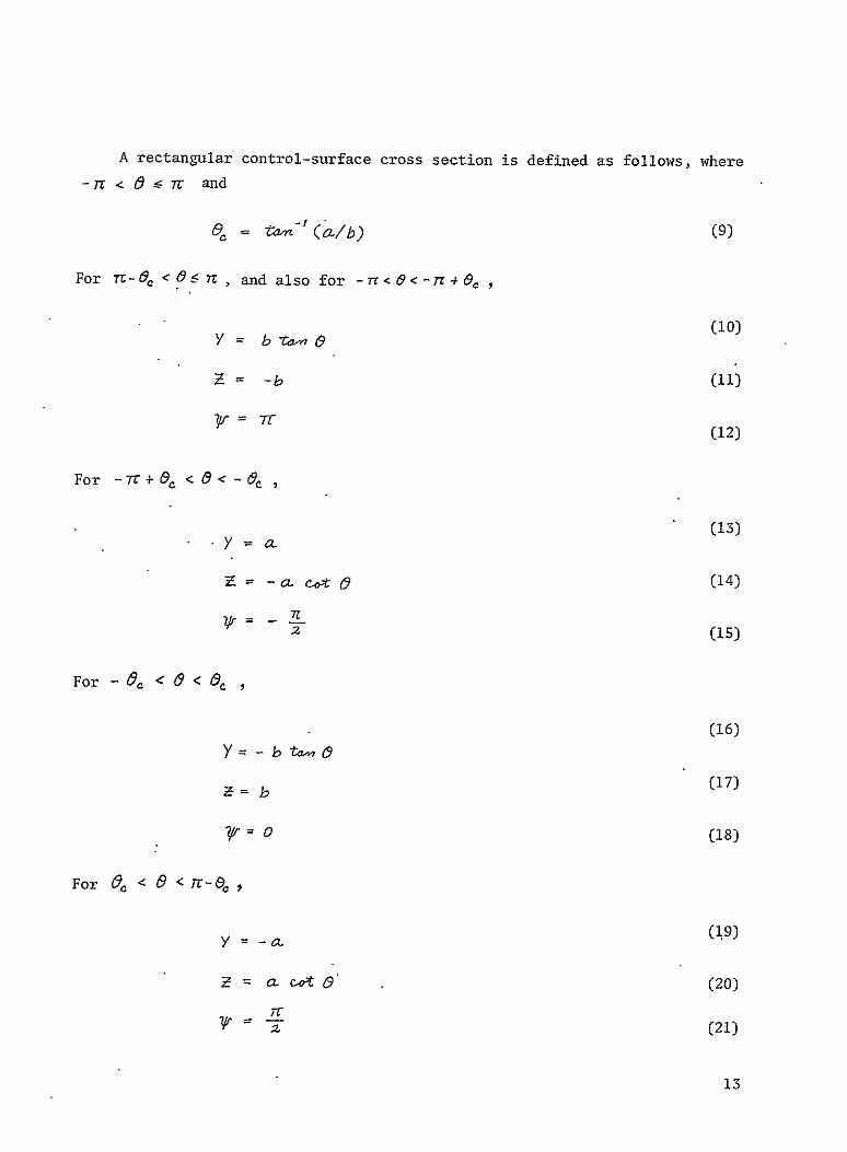
A rectangular control-surface cross section is defined as follows, where
-n < 0 7 and
&'n' b) (9)
For Tm-6 0 <c0 i5 , and also for -7T<&<-774L9.
S= -b (ii)
(12)
For -jT+G, <0'-&c
(13)
-ECLCtL (14)
7Z
For-&, 3 ,
(16)Y= - b t~4
(17)
0o (18)
For 8a < L9 <wr-&0 ,
y -a. (9)
= ac "t 0 (20)
TC7' (21)
13

Separate subroutines implementing cross sections of both elliptical and
In all the applicationsrectangular shape have been developed and checked.
described below, however, only elliptical cross sections have been considered.
General Formulation of Functional Relationships
The two-dimensional functional relationships can be formulated, in the
absence of propulsion-system efflux exiting through the control surface, in
terms of either source or vortex distributions along the control surface.
Both formulations are equivalent and for unconfined flow lead to the direct
integral relationships between the disturbance velocity components normal and
In twotangential to the control surface that are given in the Appendix.
dimensional flow about a body in ground effect, the alternative formulations
are equivalent as well, but lead in each case to different pairs of equations,
one of which is an integral equation and the other an integral evaluation
once the integral equation has been solved.
Similarly, the three-dimensional unconfined-flow functional relationships,
in the absence of the efflux intersecting the control surface, can be formu
lated in several ways. If we assume that incompressible, inviscid flow is a
suitable approximation for the region external to the control surface, the
most familiar formulation is found by considering a source distribution 6r(ZC)
over the entire control surface Y5 , whereupon the disturbance velocity
potential 0 can be written at a general field point ( X, , ), following
Hess and Smith (refs. 37-39) as
C(X: 6') 1(8'., C6'- cl')0' (22) ~r
where the primes denote the variables of integration and
r 144 Y(69)][+ (0)J (23)
14

The velocity components can be found by differentiating equation (22) with
respect to the appropriate coordinate directions. If this is done in the X,
n , t system and the appropriate limits are taken, we have on the control
surface, 2Wr
74~~~x(ZI) JJ [V) (LL) 020d~x6 69'_o' 0' d.aect
L,6 I:i(24)
a~~.= -2nro-zXo)ff (xOD)_k-U-- L(O)MC,(OtV'dO'6
2(25)
rY((0V7t ('- aoNzZ' .CO
0) C&O(19)] (&'-%r)d8'dz'
_t ot V=Y(&) (26)
The integrals in equations (24) and (26) must be evaluated in the Cauchy
principal value sense.
If the normal velocity component .r is assumed to be known on the control
surface from measurements, equation (25) is an integral equation of the second
kind and represents the classical Neumann problem of potential theory. General
numerical techniques have been developed, principally by Hess and Smith
(refs. 37-39), to solve equation (25) for arbitrary three-dimensional configu
rations. Once this equation has been solved for r , equations (24) and (26)
can be evaluated to get the other components for comparison with their
measured values. As an alternative to evaluating equation (26) for 14 , how
ever, we note that once 2rz has been evaluated from equation (24), the
potential ' can be found on the control surface by integration, namely
Jcr, 0) 0 ) d. 4 (27)
In establishing equation (27), we have made use of the fact that 4 must vanish
at infinity upstream for the flow about a three-dimensional configuration of
15
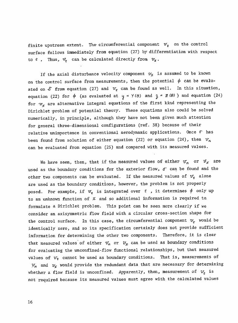
finite upstream extent. The'circumferential component -Y* on the control
surface follows immediately from equation (27) by differentiation with respect
to t Thus, 'tt can be calculated directly from 2r,.
If the axial disturbance velocity component VZ is assumed to be known
on the control surface from measurements, then the potential j can be evalu
ated on -S'from equation (27) and -Vt can be found as well. In this situation,
equation (22) for 4 (as evaluated at V = Y(&) and . = Z (e)) and equation (24)
for -r, are alternative integral equations of the first kind representing the
Dirichlet vroblem of potential theory. These equations also could be solved
numerically, in principle, although they have not been given much attention
for general three-dimensional configurations (ref. 38) because of their
relative unimportance in conventional aerodynamic applications. Once a has
been found from solution of either equation (22) or equation (24), then -V.
can be evaluated from equation (25) and compared with its measured values.
We have seen, then, that if the measured values of either v., or 7, are
used as the boundary conditions for the exterior flow, 6- can be found and the
other two components can be evaluated. If the measured values of Trt alone
are used as the boundary conditions, however, the problem is not properly
posed. For example, if V4 is integrated over t , it determines 0 only up
to an unknown function of % and so additional information is required to.
formulate a Dirichlet problem. This point can be seen more clearly if we
consider an axisymmetric flow field with a circular cross-section shape for
the control surface. In this case, the circumferential component V. would be
identically zero, and so its specification certainly does not provide sufficient
information for determining the other two components. Therefore, it is clear
that measured values of either 1r, or -U can be used as boundary conditions
for evaluating the unconfined-flow functional relationships, but that measured
values of Vtr cannot be used as boundary conditions. That is, measurements of
y. and wr would provide the redundant data that are necessary for determining
whether a flow field is unconfined. Apparently, then, measurement of -Yt is
not required because its measured values must agree with the calculated values
16

if the measured and calculated values of V, and Vz agree. Nevertheless, its
retention provides an additional indication of the degree of satisfaction of
the unconfined-flow conditions.
Multipole Expansion Procedures
Theoretical Background.- As an alternative to a full solution of
equations (24) to (26), a multipole expansion (MPE) procedure has been de
veloped along the lines that we have found so useful in two dimensions (refs.
30 and 31). The MPE is based upon fundamental solutions of Laplace's equation
and so there is no need to consider equations (22) to (26) directly. The
prod9dure, to be 4escribed fully below, basically consists of fitting one com
ponent of the measured velocity data in a series expansion of the fundamental
solutions. The coefficients of the series are then used to evaluate series
expansions for the corresponding unconfined-flow distributions of the other two
velocity components. We have found in our two-dimensional investigation that
the MPE technique has several advantages.
The principal advantage of the MPE procedure is that the calculations are
straightforward and the associated computer program is very efficient. In our
two-dimensional numerical simulations (ref. 30) of a self-correcting wind
tunnel, for example, the least-squares fit technique led to errors between the
fit and the individual data points that were far smaller than any errors
expected from experimental measurement inaccuracies. These simulations were
carried out for two different airfoil-section shapes and for several values of
the ratio of chord-to-control-surface-height. Furthermore, the MPE approach
can be adapted readily, by means of alternative subroutines in the computer
program, to any control-surface cross-sectional shape. Another advantage that
we have found useful in our two-dimensional experiments (ref. 31) is that the
MPE provides a straightforward analytic continuation from one control surface
location to another. We have found it convenient in the two-dimensional ex
periments to measure each of the two velocity components at a different
distance from the airfoil. The MPH handles this geometrical situation directly,
17

whereas an integral equation formulation, as in equations (24) or (25), would
have'to be generalized and solution would become more complicated. Finally,
the MPE tan be used, in conjunction with conventional wall-correction theory,
to assess the accuracy of the flow about the model if the functional relation
ships are not satisfied exactly.
The MPE development has been carried out for linearized compressible
flows. The Prandtl-Glauert equation has been assumed to be a valid approxi
mation-in the flow region external to the control surface. This formulation '
reduces-to-the incompressible flow case when /3 = (I- /w) goes to one,
where M. is the free-stream Mach number. The origin of-the MPE will be
assumed to coincide with the origin of the Z , , . coordinate system in
figure 1.
In a typical application of the self-correcting tunnel concept, either in
a wind tunnel or in a numerical simulation of a tunnel, measurements of the
disturbance velocity components, say v% , vz,. and tr would be made at a
number of locations on the control surface. For this discussion, we will con
sider all three components, although Ir.. is really unnecessary as discussed
above. The first step in the MPE technique is to fit either vY, or Vn. by
a series expansion in the appropriate component of fundamental singularity
solutions of the Prandtl-Glauert equation. If vx. is taken as the boundary
condition on the external flow, a least-squares fit is carried out of the form
o;J i o 13x (28)
where is the velocity component induced in the z-direction by the .h
singularity. Once the coefficients X are found from the least-squares fit,
the values of the other two components, 1r, r--,] and vt= [7], say, that
correspond to z, if the flow is unconfined, can be evaluated by
3
(29)(XO) = 0 ; 3)
18

J
where % and % are the velocity components induced in then-and th
t-directions, respectively, by the 4 singularity. These calculated values are then compared with the measured values V,, and Jt.v. If they agree the flow is unconfined, but if they do not agree, the differences are a measure
of the interference present.
Alternatively, % can be fit in a series of the form
3 0;13)(31)
whereupon Vx, [2r,,] and zv [t] are given by
S
;t(x, 60) /V (z a1.(,6 (33)C ~ p t1 3
and r and zr, must be compared with v,. and Vt. respectively.
The choice of functions in the MPH series is somewhat arbitrary. Any combination of point singularities or spatial distributions of singularities
may be used, so long as they satisfy the Prandtl-Glauert equation, are linearly independent, and are fully contained within the control surface. We have developed two separate MPE methods, which will be discussed in turn. The first
is based on point singularities and is called the original MPE, while the second,
the modified MPE, is tailored specifically for wings.
Original MPH Method and Results.- In this MPH method, we followed our
two-dimensional procedure to use a systematically defined set of point singularities that are generated from three of the basic singularities used in conventional wind-tunnel-wall correction analyses (ref. 40). These latter
19

singularities are the source, the velocity potential of which (called P, here for later convenience) is given by
4%=(- 4 (34)
the so-called infinitesimal-span horseshoe vortex representing the component
of the lift force in the j-direction, the potential of which (#,o, say) is
given by
10 [ 2 - C35)
and the infinitesimal-span horseshoe vortex representing the -component of
the lift, the potential of which ( 0., say) is given by
S-) + (36)
These three singularities can,be derived by considering a source singularity
(to, say) which satisfies the Prandtl-Glauert equation for the acceleration
potential q , namely
__ (37)
If k is differentiated with respect to _Z to find , which is then inte
grated according to the relationship which holds in steady flow between the
acceleration potential and the velocity potential, namely
WI (38)
we obtain Similarly, differentiation of 4t-with respect to and inte
gration according to equation (38) yield 1,,while differentiation with respect
to and the subsequent integration yield 95z
20

The basic set .of singularities that we have chosen, Ithen, consists of the
three singularities in equations (34) to (36) plus all of their linearly in
dependent first and second derivatives. The resulting fifteen MPE singu
larities for general, nonsymmetrical flow cases are assumed to be located at
the origin. They are presented in Table I as the velocity components
and in, the X-, V-and - directions, respectively. The -and
components can be resolved into the'y- and t-components 't and by
reference to figure 1, namely
r(Z,O; 13) - ' 0(6; t.)- )- (Z, 56) C04 P(O) (39)
The terms in the series are arranged so that the first nine terms are those
for flow configurations which are symmetrical about the Z- - plane; i..e., those
'for which % are and an6., and even functions of is odd
finction of The remaining six terms extend the analysis to general three
dimensional configurations and are those for which , and are odd
functions of I while TY. is an even function of . Therefore, symmetrical
and general configurations are, considered using "J = 9 and 15, respectively
A computer program implementing .the original MPE procedure has been.
written incorporating the subroutine for elliptical control-surface cross
sections. Preliminary checks of the program were carried out based on indi
vidual singularities-and hand calculations. A more thorough checkout has been
carried out using evaluations of the unconfined flow fields of typical wing
and body representations. -For wings; short computer programs have been
- written to evaluate the unconfined flow field at control surfaces enclosing
wings with elliptical and constant spanwise loadings. A lifting-line repre
sentation consisting of finite-span horseshoe vortices has been constructed for
this purpose following the guidelines of Hough (ref. 41). Another short pro
gram was written to evaluate the unconfined flow field at control surfaces
enclosing Rankine solids (ref. 42), which are used to represent typical body
shapes. -The results for the unconfined-flow distributions of the axial and
normal velocity components calculated with these programs are referred to as
"exact" values in.the discussion which follows, and are denoted by Vr . and
4., respectively.
21

Both circular control-surface cross sections with h/a, = 1.0 and elliptical
cross sections with b/- = 0.5 have been examined in these check cases and the
results generall-y are comparable. We will discuss here some typical results
for symmetrical configurations in incompressible flow. The nine-tem symmet
rical MPE has been used to obtain these results, but a spot check with the
general 15-term MPE shows that they are equivalent.
With the original program, wings with the ratios 6./a of span-to-control-
The results are similar for bothsurface-width of 0.25 and 0.5 were examined. =
constant and elliptical spanwise loadings. For the larger (b/i 0.5),
b/. = 0.5, the axial and normal disturbanceelliptically-loaded wing with
velocity components at the control surface, nondimensionalized in terms of 1M
the aspect ratio )R and the lift coefficient CL , are presented in figures 2
Since .lZr, andand 3, respectively,*as functions of & for two values of x/& .
v., are symmetrical about 5 = 0, results in'the cross-section plane of the
lifting line ( %/a = 0.0) are given on the right-hand sides of the figures,
while results one half-width downstream (Z/ = 1.0) are given on the left
hand sides. As can be seen from'the figures, the MPE fits to 7 zm and to V,.
are in considerable error and so lead to errors in the corresponding calculated
distributions rz, [v] and 2r, Lx.]. In the case of the smaller wing
(b /. = 0.25), on the other hand, the results are not presented because the
MPE fits as well as the calculated distributions ?rA= [zm]and ?, [vx jare
indistinguishable from the exact distributions to the scale of figures 2 and 3.
With the original program, Rankine solids with a diameter-to-length ratio
T of 0.2 also were'considered at zero angle of attack for a circular control-
Three different values of the ratio of body-length-tosurface cross section.
For thecontrol-surface-width kb/a were treated, namely 0.2, 0.5 and 1.0.
smallest body (bta = 0.2), the errors between 7z, , zm and their MPE fits,
and between r,, 7,/, and the calculated values jr., m] and ['zjj,v'n are
very small, roughly comparable to the agreement for wings with bw/a- = 0.25.
For the body with b/ = 0.5, the errors are significantly larger, roughly of
the same magnitude as for the wings with b./a, = 0.5 in figures 2 and 3. The
results for the axial and normal disturbance velocities, nondimensionalized by
22
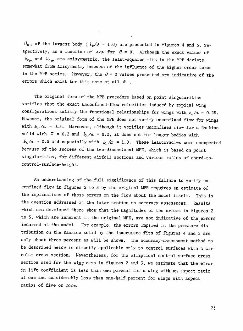
=U., of the largest body C bb/la 1.0) are presented in figures 4 and 5, re
spectively, as a function of Z/, for 6 = 0. Although the exact values of 2Y,. and 2 ,m are axisymmetric, the least-squares fits in the MPE deviate somewhat from axisymmetry because of the influence of the higher-order terms
in the MPE series. However, the 0 = 0 values presented are indicative of the
errors which exist for this case at all B
The original form of the MPE procedure based on point singularities
verifies that the exact unconfined-flow velocities induced by typical wing
configurations satisfy the functional relationships for wings with 464 /cz = 0.25. However, the original form of .the MPE does not verify unconfined flow for wings with bhlo/ = 0.5. Moreover, although it verifies unconfined flow for a Rankine
solid with V = 0.2 and 6/a = 0.2, it does not for longer bodies with
Lb la= 0.5 and especially with b./a. = 1.0. These inaccuracies were unexpected
because of the success of the two-dimensional MPE, which is based on point
singularities, for different airfoil sections and various ratios of chord-to
control-surface-height.
An understanding of the full significance of this failure to verify unconfined flow in figures 2 to S by the original MPE requires an estimate of
the implications of these errors on the flow about the model itself. This is the question addressed in the later section on accuracy assessment. Results
which are developed there show that the magnitudes of the errors in figures 2 to 5, which are inherent in the original MPE, are not indicative of the errors
incurred at the model. For example, the errors implied in the pressure dis
tribution on the Rankine solid by the inaccurate fits of figures 4 and 5 are only about three percent as will be shown. The accuracy-assessment method to
be described below is directly applicable only to control surfaces with a circular cross section. Nevertheless, for the elliptical control-surface cross
section used for the wing case in figures 2 and 3, we estimate that the error
in lift coefficient is less than one percent for a wing with an aspect ratio
of one and considerably less than one-half percent for wings with aspect
ratios of five or more.
23

Modified MPH Method and Results.- Although the accuracy-assessment results
indicate that the errors in the flow about the model are not as large as the
errors in the original MPH fits themselves, it is still important to eliminate
these inherent errors as far as possible. Consequently, a modified form of
the MPE analysis has been developed in order to extend the size of the wings
(b,/a.) which can be treated with high accuracy. No attention has been given
to extending the range of body lengths (Lb/a) which can be treated accurately
although the same principles should be applicable in that case as well.
The modified MPB has been carried out for symmetrical configurations only;
i.e., J = 9 is considered as the limit in the MPH. As mentioned earlier, the
choice of singularities in the MPE is somewhat arbitrary. Therefore, in order
to extend the MPE technique to larger h./1a values, we have replaced the in
finitesimal-span horseshoe vortex with lift in the i-direction (i.e., term 2
in Table I) by a finite-span horseshoe vortex similarly oriented. The semi
span bV of the horseshoe vortex is arbitrary, but for all examples to date,
we have chosen b. = f3' ,/2. This value matches exactly (ref. 43) the first
two terms in a multipole expansion of the velocity potential for an elliptically
loaded lifting-line representation of a wing. The strength r.of the horseshoe vortex is given by
The check cases for the modified MPE computer program have all considered
the unconfined flow about elliptically-loaded wings located within an elliptical
= control surface with b/. 0.$. The first example is for b,/o = 0.5; i.e.,
the case treated by the original MPE and presented in figures 2 and 3. The
fit and calculated values using the modified form of the MPH are indistinguishable
from the exact distributions in figures 2 and 3 so are not presented there ex
plicitly. The modified MPE thus verifies very accurately that this flow field
is unconfined and so represents a significant improvement over the original
form.
24
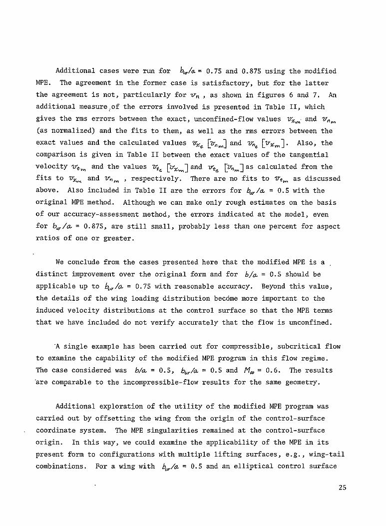
Additional cases were run for 4,/a= 0.75 and 0.875 using the modified
MPE. The agreement in the former case is satisfactory, but for the latter
the agreement is not, particularly for -v,, as shown in figures 6 and 7. An
additional measure 'of the errors involved is presented in Table II, which
gives the rms errors between the exact, unconfined-flow values lr. and in
(as normalized) and the fits to them, as well as the rms errors between the
exact values and the calculated values V. [wa,] and % [zrz.]. Also, the
comparison is given in Table II between the exact values of the tangential velocity -v-f,and the values 7= [Zr] and v B',m]as calculated from the
fits to s, and ir,m , respectively. There are no fits to Vt, as discussed
above. Also included in Table II are the errors for b4/ = 0.5 with the
original MPE method. Although we can make only rough estimates on the basis
of our accuracy-assessment method, the errors indicated at the model, even
for b,/o = 0.875, are still small, probably less than one percent for aspect
ratios of one or greater.
We conclude from the cases presented here that the modified MPE is a =distinct improvement over the original form and for b/a 0.5 should be
applicable up to 1,/o. = 0.75 with reasonable accuracy. Beyond this value,
the details of the wing loading distribution become more important to the
induced velocity distributions at the control surface so that the MPE terms
that we have included do not verify accurately that the flow is unconfined.
*Asingle example has been carried out for compressible, subcritical flow
to examine the capability of the modified MPE program in this flow regime.
The case considered was b/a. = 0.5, b,/a = 0.5 and 14 = 0.6. The results
are comparable to the incompressible-flow results for the same geometry.
Additional exploration of the utility of the modified MPE program was
carried out by offsetting the wing from the origin of the control-surface
coordinate system. The MPE singularities remained at the control-surface
origin. In this way, we could examine the applicability of the MPE in its
present form to configurations with multiple lifting surfaces, e.g., wing-tail
combinations. For a wing with b/a = 0.5 and an elliptical control surface
25
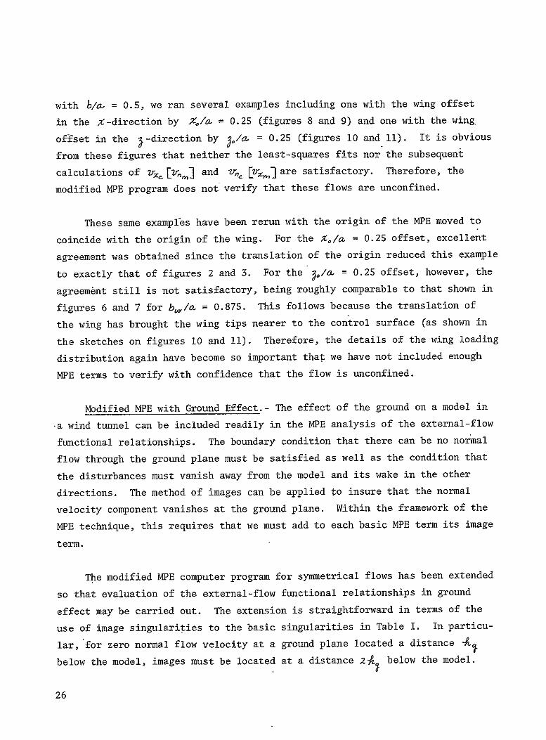
with biw = 0.5, we ran several examples including one with the wing offset
in the X-direction by Zfo. = 0.25 (figures 8 and 9) and one with the wing
= offset in the 3 -direction by o/a- 0.25 (figures 10 and 11). It is obvious
from these figures that neither the least-squares fits nor the subsequent
calculations of V., [rj and v- [Vt] are satisfactory. Therefore, the
modified MPE program does not verify that these flows are unconfined.
These same examples have been rerun with the origin of the MPE moved to
coincide with the origin of the wing. For the 9.o, = 0.25 offset, excellent
agreement was obtained since the translation of the origin reduced this example
to exactly that of figures 2 and 3. For the lo/ = 0.25 offset, however, the
agreement still is not satisfactory, being roughly comparable to that shown in
= figures 6 and 7 for bhla 0.875. This follows because the translation of
the wing has brought the wing tips nearer to the control surface (as shown in
the sketches on figures 10 and 11). Therefore, the details of the wing loading
distribution again have become so important that we have not included enough
MPE terms to verify with confidence that the flow is unconfined.
Modified MPE with Ground Effect.- The effect of the ground on a model in
,awind tunnel can be included readily in the MPH analysis of the external-flow
functional relationships. The boundary condition that there can be no normal
flow through the ground plane must be satisfied as well as the condition that
the disturbances must vanish away from the model and its wake in the other
directions. The method of images can be applied to insure that the normal
velocity component vanishes at the ground plane. Within the framework of the
MPE technique, this requires that we must add to each basic MPE term its image
term.
The modified MPE computer program for symmetrical flows has been extended
so that evaluation of the external-flow functional relationships in ground
effect may be carried out. The extension is straightforward in terms of the
use of image singularities to the basic singularities in Table I. In particu
lar,'for zero normal flow velocity at a ground plane located a distance -A
below the model, images must be located at a distance 2A below the model.
26
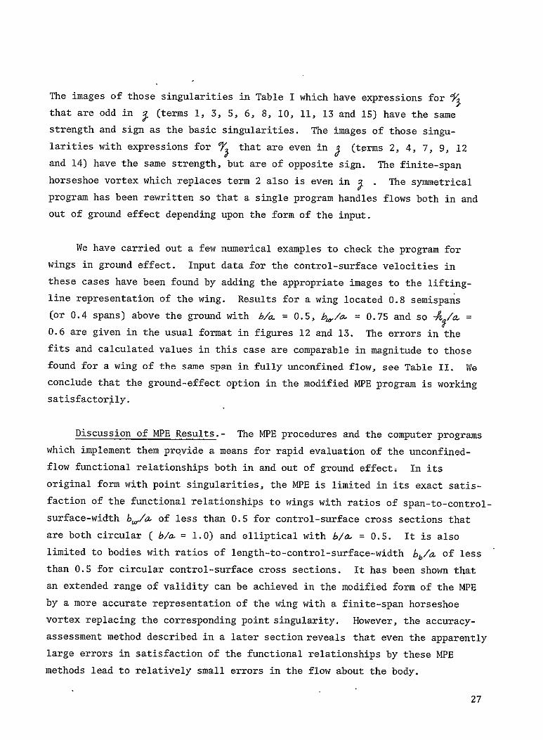
The images of those singularities in Table I which have expressions for
that are odd in i (terms 1, 3, 5, 6, 8, 10, 11, 13 and 15) have the same
strength and sign as the basic singularities. The images of those singu
larities with expressions for 7 that are even in j Cterms 2, 4, 7, 9, 12
and 14) have the same strength, but are of opposite sign. The finite-span
horseshoe vortex which replaces term 2 also is even in 5 . The symmetrical
program has been rewritten so that a single program handles flows both in and
out of ground effect depending upon the form of the input.
We have carried out a few numerical examples to check the program for
wings in ground effect. Input data for the control-surface velocities in
these cases have been found by adding the appropriate images to the lifting
line representation of the wing. Results for a wing located 0.8 semispans
(or 0.4 spans) above the ground with b/. = 0.5, bh/a = 0.75 and so -A a,=
0.6 are given in the usual format in figures 12 and 13. The errors in the
fits and calculated values in this case are comparable in magnitude to those
found for a wing of the same span in fully unconfined flow, see Table II. We
conclude that the ground-effect option in the modified MPH program is working
satisfactorily.
Discussion of MPH Results.- The MPH procedures and the computer programs
which implement them provide a means for rapid evaluation of the unconfined
flow functional relationships both in and out of ground effect. In its
original form with point singularities, the MPB is limited in its exact satis
faction of the functional relationships to wings with ratios of span-to-control
surface-width bh/o of less than 0.5 for control-surface cross sections that
are both circular ( b/a. = 1.0) and elliptical with b/. = 0.5. It is also
limited to bodies with ratios of length-to-control-surface-width kb/ of less
than 0.5 for circular control-surface cross sections. It has been shown that
an extended range of validity can be achieved in the modified form of the MPH
by a more accurate representation of the wing with a finite-span horseshoe
vortex replacing the corresponding point singularity. However, the accuracy
assessment method described in a later section reveals that even the apparently
large errors in satisfaction of the functional relationships by these MPE
methods lead to relatively small errors in the flow about the body.
27
Thus, we conclude that the form of the MPH should be tailored to the
specific model being tested for most accurate evaluation of the unconfined
flow functional relationships in an experimental situation. This is contrary
to our two-dimensional experience where a single MPE based on point singu
larities had broad applicability in theoretical studies. However, recent exz
perience in our two-dimensional experiments has revealed another weakness of
In particular, it appears that the errors between the least-squaresthe MPE.
fit and the measured data points are no longer negligible in experimental
If this is the case, these errors williterations toward unconfined flow.
reduce the accuracy of the entire self-correcting wind tunnel system. A more
thorough assessment of the implications of these errors is underway in two
dimensions.
Consequently, we believe that a more general, less configuration-tailored
method for evaluating the functional relationships is desirable. This is
necessary especially when large deformations of the trailing vortex system
occur and definitely will be required in extension of the analysis to include
the propulsion-system efflux when it exits through the control surface into
the external flow in the vicinity of the model. The development of a singu
larity distribution method, such as a source distribution or vortex lattice
procedure would provide such a general method for evaluating the functional
To this end, development of a source distribution method wasrelationships.
begun and is described next.
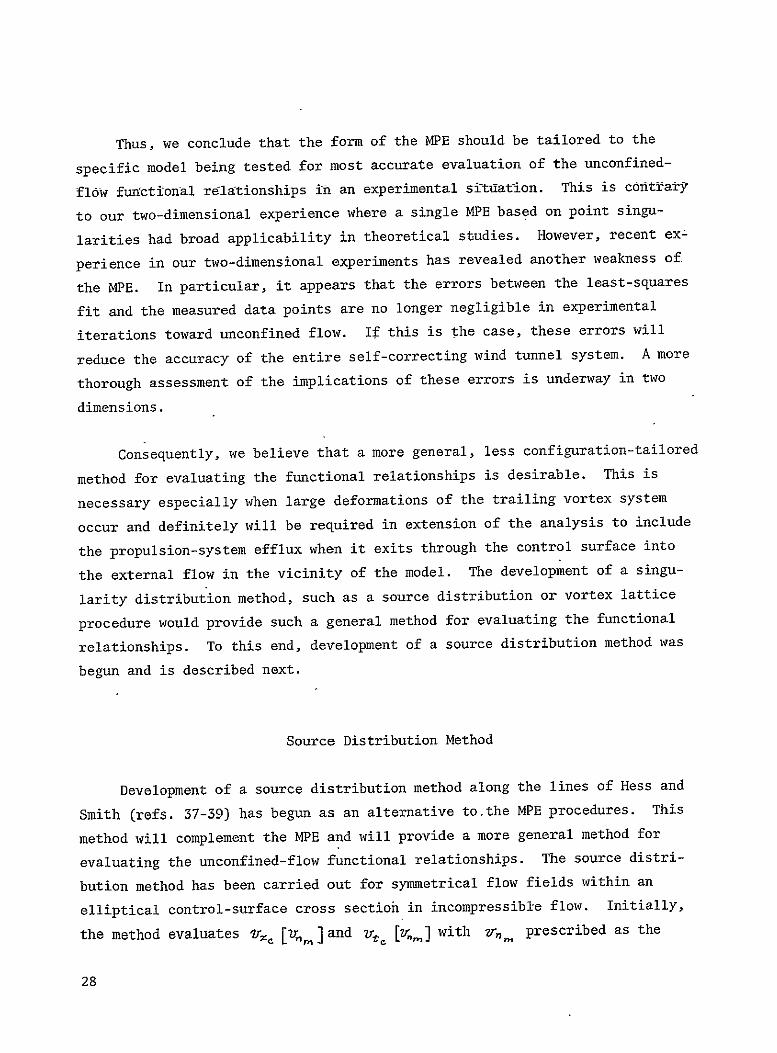
Source Distribution Method
Development of a source distribution method along the lines of Hess and
Smith (refs. 37-39) has begun as an alternative tothe MPH procedures. This
method will complement the MPE and will provide a more general method for
The source distrievaluating the unconfined-flow functional relationships.
bution method has been carried out for symmetrical flow fields within an
elliptical control-surface cross sectioh in incompressible flow. Initially,
the method evaluates Iz, [zm ]and v, R.,,] with r, prescribed as the
28
boundary condition on the control surface for nonlifting bodies. Generaliza
tions to Vx. as the boundary condition, to lifting bodies, and to compressible
flow would be the next steps in the development.
The computer program implementing the source distribution method is a
straightforward application of references 37-39 to a control surface with
elliptical cross section. The principal difference concerns the normal flow
boundary condition which is no longer dependent on the control surface shape,
but rather is a set of normal velocity measurements. In the program, the
normal velocity component ?r,, is read in over a range of & values for each
of several different z values. A cubic spline interpolation procedure is
used, first in 9 at a constant % , and then in % at constant & , to obtain
1r,. at the centroid of each elemental source panel. These interpolated values
are then the boundary conditions for determining the elemental source strengths.
Similar interpolations are made in 1r, and lftm to facilitate their comparison
with z [2r,.] and 't,[VZm]. A direct solution of the resulting set of
linear algebraic equations is used to determine the source strengths, whereupon
the desired output quantities, e.g., v [zr] and r 0,], are evaluated.
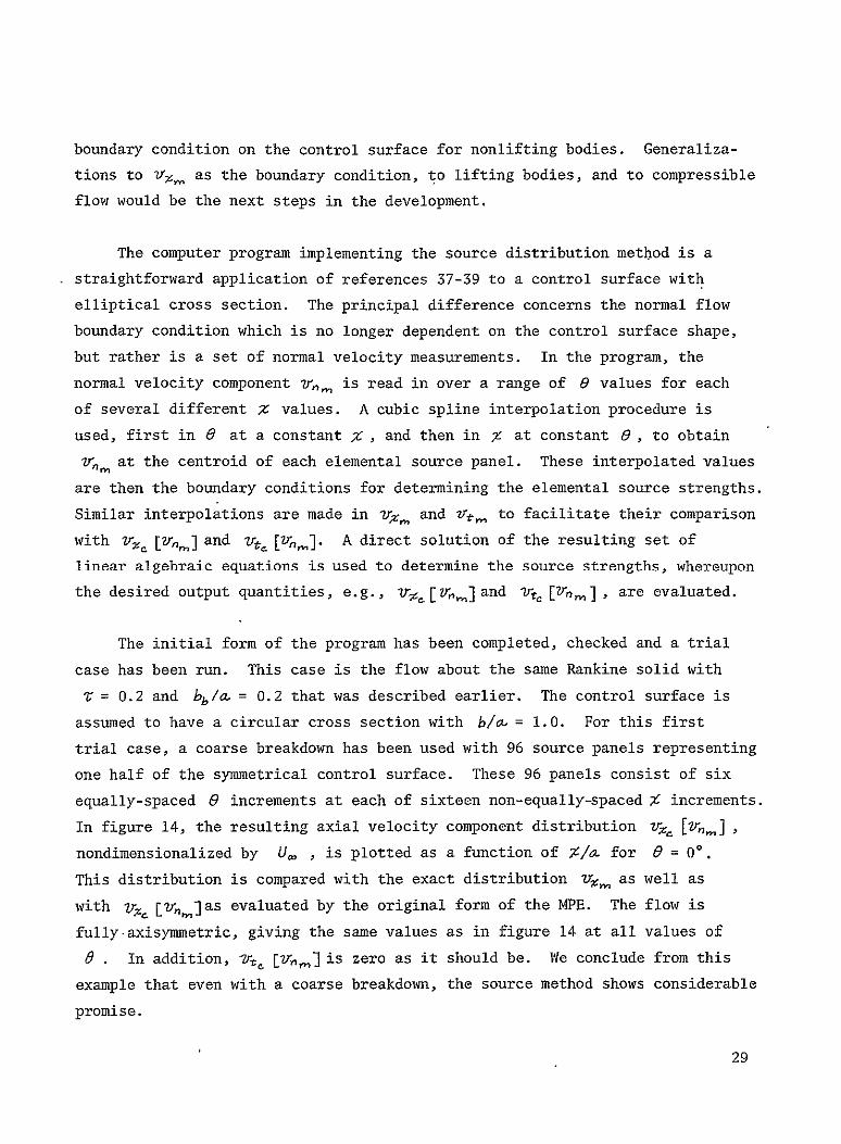
The initial form of the program has been completed, checked and a trial
case has been run. This case is the flow about the same Rankine solid with
V = 0.2 and bb/a = 0.2 that was described earlier. The control surface is =assumed to have a circular cross section with b/- 1.0. For this first
trial case, a coarse breakdown has been used with 96 source panels representing
one half of the symmetrical control surface. These 96 panels consist of six
equally-spaced e increments at each of sixteen non-equally-spaced X increments.
In figure 14, the resulting axial velocity component distribution lr Ezr[,h,]
nondimensionalized by U , is plotted as a function of %/, for 9 = 00.
This distribution is compared with the exact distribution Vrxm as well as
with 7vx, [V,']as evaluated by the original form of the MPE. The flow is
fully.axisymmetric, giving the same values as in figure 14 at all values of
9 . In addition, rt [v,.] is zero as it should be. We conclude from this
example that even with a coarse breakdown, the source method shows considerable
promise.
29

The source distribution program can be made very efficient for routine
usage after all the required generalizations are made. Once the source panel
geometry is decided upon for a given control-surface cross section (b/l), the
matrix of the normal velocity induction can be set up and inverted once and
for all (assuming that the inversion can be carried out accurately) and stored
on tape. Then each time the functional relationships for unconfined flow must
be evaluated, it would be a matter only of reading in and interpolating in the
7Xm' qrn- and Irt. data, of evaluating the source strengths from the measured
v., by use of the inverse matrix, and then evaluating 74.[r;, ]and v [v,1.
Therefore, the source distribution method is also potentially an efficient method
for verifying that a given wind tunnel flow is unconfined.
APPLICATION OF FUNCTIONAL RELATIONSHIPS TO ASSESSMENT OF WIND-TUNNEL INTERFERENCE
General
The question naturally arises-as to how accurately the unconfined-flow
functional relationships must be satisfied for the flow about the model to be
This becomes of paramount importanceinterference free in a practical sense.
in application of the concept to testing in existing conventional Wind tunnels.
For answers to this question, the flow within the tunnel must be considered as
well as the flow exterior to the control surface.
This requires that the flow within the tunnel be modeled theoretically.
Obviously, the more accurate the representation of this internal flow, the
better the accuracy question can be answered. Thus, for the type of wind
tunnel models considered in the previous section, a singularity distribution
However, a first estimate of the inaccuracyrepresentation would be desirable.
involved in failure to satisfy exactly the unconfined-flow functional relation
ships can be found by the simplified method described below. Before pre
senting this method, it should be remarked that the accuracy question must be
30
addressed ultimately experimentally. We have found this to be the case in our
two-dimensional transonic self-correcting wind tunnel (ref. 31).
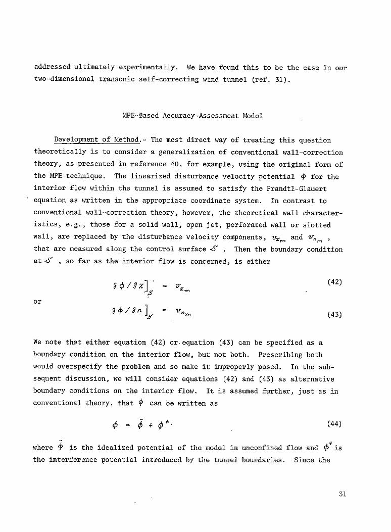
MPE-Based Accuracy-Assessment Model
Development of Method.- The most direct way of treating this question
theoretically is to consider a generalization of conventional wall-correction
theory, as presented in reference 40, for example, using the original form of
the MPE technique. The linearized disturbance velocity potential 4 for the
interior flow within the tunnel is assumed to satisfy the Prandtl-Glauert
equation as written in the appropriate coordinate system. In contrast to
conventional wall-correction theory, however, the theoretical wall character
istics, e.g., those for a solid wall, open jet, perforated wall or slotted
wall, are replaced by the disturbance velocity components, vzr and 2,, ,
that are measured along the control surface <V . Then the boundary condition
at-6" , so far as the interior flow is concerned, is either
a /8z]s" = V'Z , (42)
or 4/On] I=nm (43)
We note that either equation (42) or.equation (43) can be specified as a
boundary condition on the interior flow, but not both. Prescribing both
would overspecify the problem and so make it improperly posed. In the sub
sequent discussion, we will consider equations (42) and (43) as alternative
boundary conditions on the interior flow. It is assumed further, just as in
conventional theory, that 4 can be written as
4 0*- (44)
where ' is the idealized potential of the model in unconfined flow and O is
the interference potential introduced by the tunnel boundaries. Since the
31

is assumed to satisfy the Prandtl-Glauert equation,idealized potential
also must satisfy it.
The analysis will be carried through first for the 14,! boundary condition,
equation (42)', which becomes, using equation (44),
a~/8]v - a#vxL.(45)
At this point, we continue to follow conventional correction theory by ex-
This is in terms of the basic singularities of reference
40. pressing
equivalent in our PE terminology, to writing
Oi/Z]¢ J; C: (46)
are determined by geometrical and measured characwhere the coefficients C
For example, the terms for J = 3 teristics of the model being tested.
are considered for symmetrical configurations and are,
generally (ref. 40)
respectively; the source whose strength is proportional to the measured drag
(wake blockage), namely
(47)a'U.CO15
-T, is the reference area of the model; where CD is the drag coefficient and
the b-directed infinitesimal-span.horseshoe vortex, whose strength is pro
portional to the measured lift (lift interference), namely
C L /3 (48)
and the upstream-directed doublet, whose strength is proportional to the model
volume V (solid blockage), namely
(49)
32

In our generalization of classical correction theory, we also expand Irz
in the MPE fit by equation (28). Then combining equations (28), (45) and (46),
we have as the boundary condition on the interference potential.
80*lz''= J1 (i-C. ) (50)
We note at this point that the conventional open-jet boundary condition, namely
34'/6Z] = 0, is the same as equation (42) with vz,= 0, so that 0* for an
open jet would satisfy equation (50) with X = 0 for all
The correction procedure thus would proceed as follows. The experiment
would be run and all appropriate quantities would be measured, both on the
model (CL , CD ) and at the control surface (v7). From the measured data,
the )X and C* would be determined. Then results of conventional open-jet
correction theory would be used directly to determine interference velocities
at the model, with C replaced by CJ-X'
Alternatively, if v,, is measured at , instead of vXr , a similar
analysis can be carried out. In this case, the , , boundary condition, equation (43), becomes
-Oln Ot5rn0 (51)
We again express P in terms of conventional correction theory, namely
J n c' I (52)
where the C are still given in equations (47) to (49) for J = 3. The MPE
expansion fit in equation (31) then can be combined with equations (51) and
(52) to give
*J
8- (53)
33
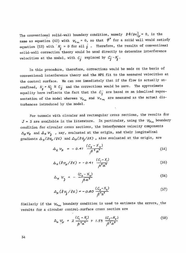
= dc/,nd3 0, is theThe conventional solid-wall boundary condition, namely
* for a solid wall would satisfysame as equation (43) with r,. = 0, so that
. Therefore, the results of conventionalequation (53) with N = 0 for all I
solid-wall correction theory would be used directly to determine interference
replaced by C -IVvelocities at the model, with r II Y V
In this procedure, therefore, corrections would be made on the basis of
conventional interference theory and the MPE fit to the measured velocities at
the control surface. We can see immediately that if the flow is actually un
confined, X = Ni Cj and the corrections would be zero. The approximate1
are based on an idealized repreequality here reflects the fact that the C
and v., are measured as the actual dissentation of the model whereas ire.
turbances introduced by the model.
For tunnels with circular and rectangular cross sections, the results for
J = 3 are available in the literature. In particular, using the 7Y, boundary
condition for circular cross sections, the interference velocity components
say, evaluated at the origin, and their longitudinalA tz and A% 2r, ,
gradients A(dirz,/8Z) and Z(y, also evaluated at the origin, are
A 0.41 (C9 -x z /9/ 3- L3 (54)
A~(Ov-/ZX) = - (.C 4J (55)
(56)(Ca- XA()
(57)488/0z -O.a0 (C9- X2)2
Similarly if the -v,. boundary condition is used to estimate the errors, the
results for a circular control-surface cross section are
AnAc1 -I) (c,-,v3 ) (58)
3/3%/
34
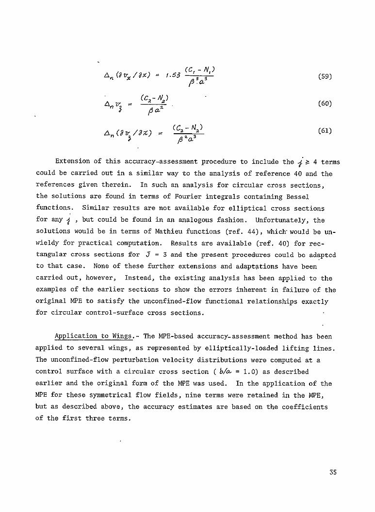
(C,-A/,) An(3tr~/ax) = /.53 (C N (59)
Sa
a(c2 2) (60)
A,(9zrq(- N,) (61)
Extension of this accuracy-assessment procedure to include the 4 terms
could be carried out in a similar way to the analysis of reference 40 and the
references given therein. In such an analysis for circular cross sections,
the solutions are found in terms of Fourier integrals containing Bessel
functions. Similar results are not available for elliptical cross sections
for any , but could be found in an analogous fashion. Unfortunately, the
solutions would be in terms of Mathieu functions (ref. 44), which"would be un
wieldy for practical computation. Results are available (ref. 40) for rec
tangular cross sections for 5 = 3 and the present procedures could be adapted
to that case. None of these further extensions and adaptations have been
carried out, however, Instead, the existing analysis has been applied to the
examples of the earlier sections to show the errors inherent in failure of the
original MPE to satisfy the unconfined-flow functional relationships exactly
for circular control-surface cross sections.
Application to Wings.- The MPE-based accuracy-assessment method has been
applied to several wings, as represented by elliptically-loaded lifting lines.
The unconfined-flow perturbation velocity distributions were computed at a
control surface with a circular cross section ( b/a- = 1.0) as described
earlier and the original form of the MPE was used. In the application of the
MPE for these symmetrical flow fields, nine terms were retained in the MPE,
but as described above, the accuracy estimates are based on the coefficients
of the first three terms.
35

In this lifting-line representation of the wings, C, and C3 are zero
N. have beenidentically and from the MPE fit to the data, X, , X 3 , N, and
calculated to be zero. Therefore, the interference velocity components in
duced at the origin (midspan of the lifting line) are, from equations (54) to
(61), the upwash A v, and its gradient in the %-direction A(9 /X). For
elliptically-loaded, flat, untwisted wings with an ideal lift-curve slope of
2Tr, the lift coefficient is given by (ref. 45)
(62)CL
Alternatively, from equation (48),.we have
2 TZ,R CZ (63)
'C, b-1S
where the definition of the aspect ratio has been used. The expressions for
the -component of the interference velocity can be related to an angle of
attack error 4a, and an effective angle of attack error AM, due to a
parabolic-are camber effect, by
XAXa (Ca- XZ) (64)
)bAr X;2b',(Cz-X (65)
2U R A / 5 U 0 "R
for the vr. boundary condition, and by
.~ (66)Ana-, C2
bar. b6/ (C - N (67)
1AM 2U0fr An (ardi-v =x 3 (67)a
for the ?t,, boundary condition. If Acc and Am. are positive, they imply
that the effective angle of attack of the model in the tunnel is larger than
C. is requiredthe geometric angle of attack. Thus a negative increment in
36

to interpret the measured data correctly. This increment is given by
equation (62) as
2 7r )RAx a )(0A 4 =- - (68)
2+/3
Combining equations (63) to (68), we obtain expressions for the errors based
on jr.. and v,. , respectively, as
ACL[] -3 k -) (69)
C-
The errors that are implied in the lift coefficient by failure of the
original MPE to satisfy the functional relationships exactly have been evaluated
by equations (69) and (70) for some incompressible flow cases. They are the
errors inherent in the original form of the MPE for a given b./. The wings
treated have aspect ratios R of 1, 5 and 10 and ratios of span-to-control
surface-width b/a of 0.2, 0.4, 0.6 and 0.8. The results are presented in
Table III. As can be seen, the errors are less than 1% in all cases. Also,
there is a difference in sign as well as magnitude between the errors based
on -e. and those based on zr,,. This provides an additional indication of
the errors inherent in the original form of the MPE. Overall, the errors are
so small that the effect at the model is negligible and so the inherent failure
to satisfy the functional relationships exactly using the MPE is not important
for the geometrical range considered.
The advantages offered by the self-correcting wind tunnel can be seen
quantitatively as follows. For the most severe geometry in Table III, namely
AR = 1 and bh/eI = 0.8, the error in a solid-wall wind tunnel of circular
cross section would be AC,/C = -0.299; i.e., an error of about thirty per
cent. If the walls of the tunnel can be adjusted so that the t, , distribution
37

is within ±10% of'the unconfined-flow values, then (1- >) will be approxi
about three percent.mately ±0.1 and so AC,/4 will be only about ±0.03; i.e.,
Application to Bodies.- The MPE-based accuracy-assessment method also has
been applied to several axisymmetric bodies at zero angle of attack as repre
sented by Rankine solids of diameter-to-length ratio V of 0.2. The uncon
fined-flow distributions were computed at a control surface with a circular
cross section (b/a = 1.0) as described earlier and the original form of the
MPE was used. As for the wings, nine terms in the MPE were used and the
accuracy estimates were based on the first three.
For the Rankine solids, C, and C. are zero identically and from the MPB
fit to the data, X, X2 , N, and N, have been calculated to be zero. More
over, since the gradients of the axial velocity in the z-direction are inde
pendent of C. , X3 and N3 , then the only nonzero interference velocity com
ponents induced at the origin (center of the body) from equations (54) to (61)
are the axial components Air,. If Avx is positive, it implies that the
than the freestream velocity.effective axial velocity at the model is larger
Consequently, a negative increment in pressure coefficient C, is required to
interpret the measured data correctly. This increment is related to A Vx by
- - -I (71)
which becomes, neglecting higher-order terms,
Ag -2A(t /U) (72)
Cr
For Rankine solids, the volume is given by
(73)V =zmb5T
where T is a function of the diameter-to-length ratio V given implicitly by
T = v (r+ z'- T)"/ . Combining equations (49), (54), (58), (72) and (73)
gives
38

AXCO o.41 (b,/a) 3 'T t Q- 73 (74)
CP / 3
Ac 1.55(b/a) T2
Cr
The errors that are implied in the pressure coefficients on a Rankine
solid by the inherent failure of the original MPE to satisfy the unconfined
flow functional relationships exactly have been evaluated using equations (74)
and (75). The Rankine solids considered have u = 0.2 (and so T = 0.191928)
and lengths bb/a = 0.2, 0.5 and 1.0. The results for incompressible flow are
given in Table IV. The errors here are larger than they are for the wing cases
in the previous section, reaching nearly three percent for b./a = 1.0. There
is a difference in sign as well as magnitude here, too. Nevertheless, the
effect of the inherent failure of the MPE to satisfy the unconfined-flow
functional relationships exactly has a relatively small effect except for the
largest body size considered here. Clearly, a modified MPE for treating bodies
of this size could be developed, as was the modified MPE for treating wings.
Improved Methods
The simplified method based on the original MPE and classical correction
theory has proved useful in assessing the accuracy of the flow about the model
for control surfaces with circular cross sections. As seen from the examples,
however, the inaccuracies in the MPE fit sometimes give indicated errors of
opposite signs depending on whether the axial or normal component of the dis
turbance velocity is used as the boundary condition. Thus, the method seems
best suited only for making rough estimates of the errors introduced by wall
interference but is not suitable for actual data correction purposes. Ex
tension to other cross-section shapes could be made and it also might be
possible to extend the analysis to make use of the modified MPE where the point
singularity representing the lift is replaced by a horseshoe vortex of finite
span.
39

The real requirement for assessing the accuracy in the flows about models,
however, is for a better representation of the interior flow within the test
section. This need could be served best, probably, by combining a lifting
surface representation of wing-fuselage models with a source distribution method
of representing the control surface. The source distribution method developed
above for evaluating the functional relationships in the exterior flow could
be adapted for use in the interior flow. Such a model would provide more
accurate assessments of the errors at models when the functional relationships
are not satisfied exactly. Moreover, the assessments could be used further to
provide corrections to the data. In this way, the measured values of the dis
turbance velocity components at the control surface would be used as the boundary
conditions on the interior flow instead of assumed wall characteristics. Use
of measured data is especially important for ventilated test sections because
it has been shown recently by several investigators, for example Vidal and
Rae (ref. 46), that the conventional wall boundary conditions for these test
sections (as used in reference 40, for example), are not representative of the
actual wall behavior. Therefore, use of the measurements with an accurate
interior flow representation could eliminate the present uncertainty in calcu
lating wall-interference corrections, especially in ventilated test-sections.
CONCLUDING REMARKS
This study on the application of the adaptive-wall, or self-correcting,
wind tunnel concept to testing in fully subsonic, three-dimensional flows has
led to the following concluding remarks.
1. The control surface at which flow disturbances are measured generally
should have a height-to-width ratio less than one for greatest applicability
both in and out of ground effect. Elliptical and rectangular shapes are
suitable choices for the control-surface cross section, which need not have
the same shape as that of the tunnel. Formulation of the unconfined-flow
40
functional relationships shows that the axial disturbance velocity component
and the component normal to the control surface are sufficient for the re
dundant measurements. The remaining orthogonal component tangential to the
control surface cannot be used because it is not independent of-the axial
component.
2. The original multipole expansion (MPE) procedure based on point
singularities in three dimensions does not evaluate the functional relation
ships accurately over as wide a range of model-to-control-surface-size as does
its two-dimensional counterpart. Modifications to the MPE by replacing
selected point singularities with singularity distributions can tailor the
MPE procedure to particular model configurations. For wings, the modified
MPE developed here is accurate over a significantly larger range of span-to
control-surface-width. A different approach based on a distribution of source
panels representing the control surface offers promise of an accurate,
efficient, and less configuration-oriented way of evaluating the functional
relationships
3. A procedure for estimating the interference at the model when the
functional relationships are not satisfied exactly has been developed for
circular control surfaces. It uses the disturbance velocity measurements, the
MPE evaluation and classical wall-correction theory. .Applications of this
procedure show that for a given magnitude of error in satisfaction of the
functional relationships, the magnitude of the interference at the model is
much less. Therefore, achievement of a given accuracy in the approach to
interference-free flow at the model imposes a less severe requirement on the
accuracy in the satisfaction of the functional relationships.
4. Development of a suitable representation of the propulsion-system
efflux outside the control surface is the next important step required to
apply the concept to V/STOL testing. Development of more accurate simulations
of the flow within the control surface is a necessary step for applications to
existing tunnels. These simulations would permit development of improved
41
correction procedures, especially for ventilated tunnels for which the wall
boundary conditions are not well founded. Finally, development of experi
mental procedures, particularly the meashrement techniques, should be carried
out for use in both existing and future tunnels.
42

APPENDIX
THE CONCEPT OF A SELF-CORRECTING WIND TUNNEL
Unconfined Flow
An ideal to strive toward would be a V/STOL tunnel that would always
adjust itself to eliminate the constraining effects of its boundaries, for any
configuration tested at any Angle of attack and/or sideslip, for any deflection
angle of the propulsion-system efflux, and at any flight speed from hover
through transition to cruise. This ideal tunnel could be approached if it were
possible to sense departures from unconfined-flow conditions in the working
section and to modify the tunnel geometry accordingly, until the readings of
appropriate sensors tonfirm that an unconfined-flow pattern exists in the
working section, whereupon test data would be read and recorded. It seems
clear that this could be done, in principle, by changing the shape of the
tunnel boundary, for unconfined-flow conditions could always be achieved by
adjusting the walls to the configuration of the stream surfaces of unconfined
flow past the given model. Another possibility would be to change the effec
tive shape of the tunnel boundary by appropriate distributions of tunnel-wall
porosity and plenum pressure behind the walls.- In either case, the possibility
of providing active control of the flow by wall adjustments leads us to the
concept of a self-correcting, or adaptive-wall, wind tunnel (ref. 29).
The essential basis of the scheme envisioned is that unconfined-flow con
ditions in the working section can be determined by means of the readings of
suitably placed sensors within the airstream. Let figure 15(a) represent a
V/STOL configuration in an unbounded stream of given velocity U . Let the
space surrounding this vehicle consist of an interior region, I, and an
exterior region, II, where the boundary Z between I and II is an imaginary
one, located near the proposed wind-tunnel boundary but having no effect on
43
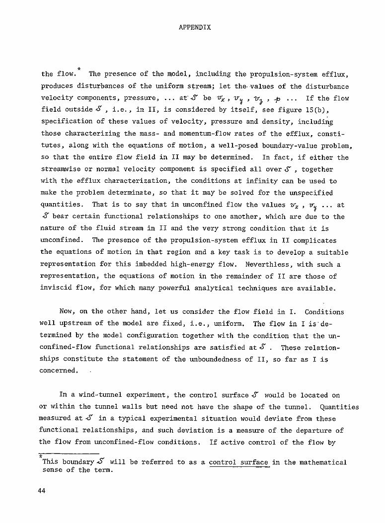
APPENDIX
the flow. The presence of the model, including the propulsion-system efflux,
produces disturbances of the uniform stream; let the-values of the disturbance
velocity components, pressure, ... at-J5 be Vzr , v- , r., _p ... If the flow
field outside S , i.e., in II, is considered by itself, see figure 15(b),
specification of these values of velocity, pressure and density, including
those characterizing the mass- and momentum-flow rates of the efflux, consti
tutes, along with the equations of motion, a well-posed boundary-value problem,
so that the entire flow field in II may be determined. In fact, if either the
streamwise or normal velocity component is specified all over-S , together
with the efflux characterization, the conditions at infinity can be used to
make the problem determinate, so that it may be solved for the unspecified
quantities. That is to say that in unconfined flow the values ?vz , ? ... at
J3 bear certain functional relationships to one another, which are due to the
nature of the fluid stream in II and the very strong condition that it is
unconfined. The presence of the propulsion-system efflux in II complicates
the equations of motion in that region and a key task is to develop a suitable
representation for this imbedded high-energy flow. Neverthless, with such a
representation, the equations of motion in the remainder of II are those of
inviscid flow, for which many powerful analytical techniques are available.
Now, on the other hand, let us consider the flow field in I. Conditions
well upstream of the model are fixed, i.e., uniform. The flow in I is'de
termined by the model configuration together with the condition that the un
confined-flow functional relationships are satisfied at J . These relation
ships constitute the statement of the unboundedness of II, so far as I is
concerned.
In a wind-tunnel experiment, the control surface 5' would be located on
or within the tunnel walls but need not have the shape of the tunnel. Quantities
measured atc5Y in a typical experimental situation would deviate from these
functional relationships, and such deviation is a measure of the departure of
the flow from unconfined-flow conditions. If active control of the flow by
This boundary 5 will be referred to as a control surface in the mathematical sense of the term.
44

APPENDIX
the walls is available, the flow can be adjusted until the existence of free
flight conditions within the tunnel is signalled by the fact that the proper
functional relationships exist among the quantities measured at -8'.
The principle involved here may be illustrated by a simple example:
suppose the flow field is one of linearized, two-dimensional, compressible,
irrotational flow about an arbitrary body without propulsion-system efflux
(figure 16). Under these conditions the Prandtl-Glauert equation is applicable.
If, in two dimensions, we locate the ends of the control surface S infinitely
far upstream and downstream, -8 becomes two infinite lines, here located at
I is the region j f < A and II is the entireregion 131>- .
The upper and lower parts of II can be considered independently of one another.
If z(Z, ) and vz(X,.) are the disturbance velocity components at any
point in the flow field, then the flow will be unconfined in I if the following
equations, which are equivalent (see reference 30, for example), are satisfied
along the two branches of <5 ; namely
= ir (,±4) dzr (Z,+A 1f (76)
%(,, ±-)= ± ff= t' (77)
To achieve interference-free flow in I, zr and 5j are measured alongz
the control surfaces, say by means of the static pressure and flow inclination.
Then, active wall control of the flow is applied until equations (76) and (77)
are found to be satisfied to a suitable degree of accuracy on the control
surfaces at =±A . The flow conditions in I are then unconfined.
The logic of the self-correcting wind tunnel scheme is contained in the
flow chart of figure 17. Basically, the scheme is an iterative one as shown.
First, a flow field is set up and the disturbance velocity components, Wz,,
and V., say, are measured along the control surfaces. The functional re
lationships in II are then evaluated to determine those distributions along Sf
45
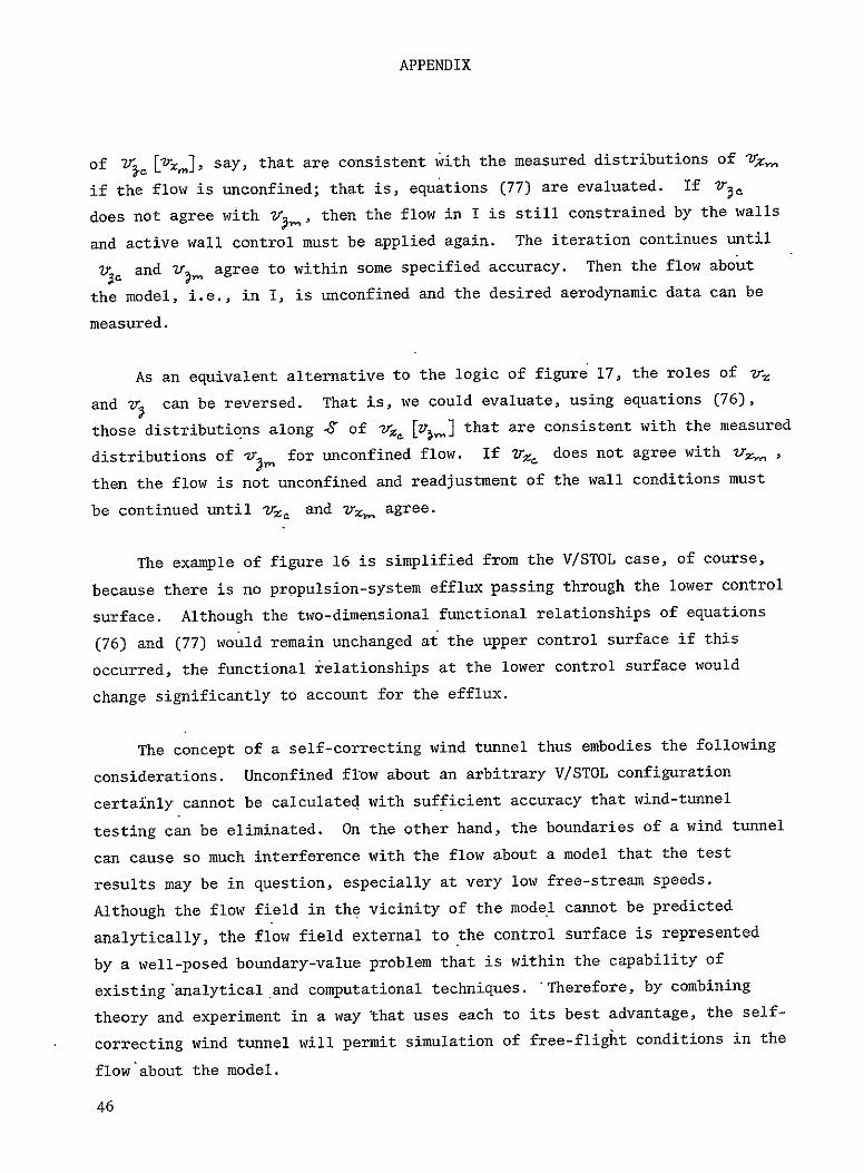
APPENDIX
of 5 [ Zr], say, that are consistent with the measured distributions of %cm
if the flow is unconfined; that is, equations (77) are evaluated. If ,
does not agree with 71,, then the flow in I is still constrained by the walls
and active wall control must be applied again. The iteration continues until
z2r and i, agree to within some specified accuracy. Then the flow about
the model, i.e., in I, is unconfined and the desired aerodynamic data can be
measured.
As an equivalent alternative to the logic of figure 17, the roles of zr,
and , can be reversed. That is, we could evaluate, using equations (76),
those distributions along 3fof -v [v] that are consistent with the measured
distributions of V,. for unconfined flow. If ?rz, does not agree with -&r,
then the flow is not unconfined and readjustment of the wall conditions must
be continued until tz, and trz. agree.
The example of figure 16 is simplified from the V/STOL case, of course,
because there is no propulsion-system efflux passing through the lower control
surface. Although the two-dimensional functional relationships of equations
(76) and (77) would remain unchanged at the upper control surface if this
occurred, the functional relationships at the lower control surface would
change significantly to account for the efflux.
The concept of a self-correcting wind tunnel thus embodies the following
Unconfined flow about an arbitrary V/STOL configurationconsiderations.
certainly cannot be calculated with sufficient accuracy that wind-tunnel
testing can be eliminated. On the other hand, the boundaries of a wind tunnel
can cause so much interference with the flow about a model that the test
results may be in question, especially at very low free-stream speeds.
Although the flow field in the vicinity of the model cannot be predicted
analytically, the flow field external to the control surface is represented
by a well-posed boundary-value problem that is within the capability of
existing'analytical and computational techniques. 'Therefore, by combining
theory and experiment in a way that uses each to its best advantage, the self
correcting wind tunnel will permit simulation of free-flight conditions in the
flow about the model.
46

APPENDIX
Ground tffect
The same basic principles would hold if it were desired to determine the
effect of the ground on a wind-tunnel model in a self-correcting wind tunnel.
In fully unconfined flow, the flow disturbance quantities must vanish at an
infinite distance in all directions from the model and its trailing vortex
wake. In the presence of the ground, however, the disturbances must vanish
far away from the model and its wake in all directions except below the model
where the flow velocity normal to the ground must be zero everywhere along the
ground plane. For ground simulation in a self-correcting wind tunnel, the
control surface must be entirely above the desired ground-plane location.
Then the external~flow functional relationships in ground effect can be derived
in a similar fashion to those for fully unconfined flow providing that the
normal-flow boundary condition is applied at the ground location.
47

REFERENCES
1. Mort, K.W.; Kelly, M.W.; and Hickey, D.H.: The Rationale and Design Features for the 40-by 80-/80-by 120-Foot Wind Tunnel. Paper No. 9 AGARD Conference Proceedings No. 174 on Windtunnel Design and Testing Techniques (London, England), 6-8 Oct. 1975.
2. Rae, W.H., Jr.: Limits on Minimum Speed V/STOL Wind-Tunnel Tests. Journal of Aircraft, vol. 4, no. 3, May-June 1967, pp. 249-254.
3. Rae, W.H., Jr.; and Shindo, S.: Comments on V/STOL Wind Tunnel Data at Low Forward Speeds. Proceedings Third Calspan/AVLABS Symposium on Aerodynamics of Rotary Wing .and V/STOL Aircraft, vol. II, Buffalo, N.Y., June 1969.
4. Rae, W.H., Jr.; and Shindo, S.: An Experimental Investigation of Wind Tunnel Wall Corrections and Test Limits for V/STOL Vehicles. University of Washington, Department of Aeronautics and Astronautics Report 73-2, July 12, 1973, AD764255.
S. Lazzeroni, F.A.; and Cary, L.W.: Problems Associated with Wind Tunnel Tests of High Disk Loading Systems at Low Forward Speeds. Proceedings Third Calspan/AVLABS Symposium on Aerodynamics of Rotary Wing and V/STOL Aircraft, vol. II, Buffalo, N.Y., June 1969.
6. Tyler, R.A.; and Williamson, R.G.: Experience with the NRC 10 Ft. x 20 Ft. V/STOL Propulsion Tunnel - Some Practical Aspects of V/STOL Engine Model Testing. Canadian Aeronautics and Space Journal, vol. 18, no. 9, Sept. 1972, pp. 191-199.
7. -Wickens, R.; South, P.; et al: Experimental Developments in V/STOL Wind Tunnel Testing at the National Aeronautical Establishment. Canadian Aeronautics and Space Journal, vol. 19, no. 4, April 1973, pp. 145-154.
8. Cull, M.J.: V/STOL Wind Tunnel Model Testing: An Experimental Assessment of Flow Breakdown Using a Multiple Fan Model. Paper No. 43, AGARD
Conference Proceedings No. 174 on Windtunnel Design and Testing Techniques (London, England), 6-8 Oct. 1975.
9. Heyson, H.H.: Jet-Boundary Corrections for Lifting Rotors Centered in Rectangular Wind Tunnels. NASA TR R-71, 1960.
10. Heyson, H.H.: Linearized Theory of Wind-Tunnel Jet-Boundary Corrections and Ground Effect for VTOL-STOL Aircraft. NASA TR R-124, 1962.
11. Heyson, H.H.: The Flow Throughout a Wind Tunnel Containing a Rotor with a Sharply Deflected Wake. Proceedings Third Calspan/AVLABS Symposium on Aerodynamics of Rotary Wing and V/STOL Aircraft, vol. II, Buffalo, N.Y., June 1969.
48

12. Heyson, H.H.: General Theory of Wall Interference for Static Stability Tests in Closed Rectangular Sections and in Ground Effect. NASA TR R-364, 1971.
13. Lo, C.F.; and Binion, T.W., Jr.: A V/STOL Wind-Tunnel Wall Interference Study. Journal of Aircraft, vol. 7, no. 1, Jan.-Feb. 1970, pp. 51-57.
14. Lo. C.F.: Wind-Tunnel Boundary Interference on a V/STOL Model. Journal of Aircraft, vol. 8, no. 3, March 1971, pp. 162-167.
15. Lo, C.F.: Test Section for a V/STOL Wind Tunnel.' Journal of Aircraft, vol. 7, no. 4, July-Aug. 1970, pp. 380-382.
16. Kraft, E.M.; and Lo, C.F.: A General Solution for Lift Interference in Rectangular Ventilated Wind Tunnels. AIAA Paper No. 73-209, Jan. 1973.
17. Kraft, E.M.: Analytical Study of Ventilated Wind Tunnel Boundary Interference on V/STOL Models Including Wake Curvature and Decay Effects. Air Force AEDC-TR-74-51, Nov. 1974.
18. Joppa, R.G.: Wind Tunnel Interference Factors for High-Lift Wings in Closed Wind Tunnels. NASA-CR-2191, Feb. 1973.
19. Heyson, H.H.: Theoretical Study of the Use of Variable Geometry in the Design of Minimal-Correction V/STOL Wind Tunnels. NASA TR-R-318, 1969.
20. Wright, R.H.: Test Sections for Small Theoretical Wind-Tunnel-Boundary Interference on V/STOL Models. NASA TR R-286, 1968.
21. Kroeger, R.A.; and Martin, W.A.: The Streamline Matching Technique for V/STOL Wind Tunnel Corrections. AIAA Paper No. 67-183, Jan. 1967.
22. Kroeger, R.A.: Wind Tunnel Design for Testing V/STOL Aircraft in Transition Flight. Air Force, AEDC TR-72-119, Sept. 1972.
23. Binion, T.W., Jr.: An Investigation of Several Slotted Wind Tunnel Wall Configurations with a High Disc Loading V/STOL Model. Air Force AEDC TR-71-77, 1971.
24. Binion, T.W., Jr.: An Experimental Study of Several Wind Tunnel Wall Configurations Using Two V/STOL Model Configurations. Report No. AEDC-TR-75-36, Arnold Engineering Development Center, July 1975.
25. Grunwald, K.J.: Experimental Investigation of the Use of Slotted Test-Section Walls to Reduce Wall Interference for High-Lift-Model Testing. NASA TN D-6292, 1971.
26. Parker, A.G.: Use of Slotted Walls to Reduce Wind-Tunnel Boundary Corrections in Subsonic Flow. AIAA Journal, vol. 12, no. 12, Dec. 1974, pp. 1771-1772.
49

27. Bernstein, S.; and Joppa, R.G.: Development of Minimum Correction Wind Tunnels. J. Aircraft, vol. 12, no. 4, April 1976, pp. 243-247.
28. Bernstein, S.; and Joppa, R.G.: Reduction of Wind Tunnel Wall Interference by Controlled Wall Flow. NASA-CR-2654, March 1976.
29. Sears, W.R.: Self-Correcting Wind Tunnels. (The Sixteenth Lanchester Memorial Lecture). The Aeronautical Journal, vol. 78, no. 758/759, Feb./March 1974, pp. 80-89; also Calspan Reports Nos. RK-5070-A-2, July 1973 and RK-5070-A-4, Oct. 1975.
30. Erickson, J.C., Jr.; and Nenni, J.P.: A Numerical Demonstration of the Establishment of Unconfined-Flow Conditions in a Self-Correcting Wind Tunnel. Calspan Report No. RK-5070-A-l, Nov. 1973.
31. Vidal, R.J.; Erickson, J.C., Jr.; and Catlin, P.A.: Experiments with a Self-Correcting Wind Tunnel. Paper No. 11, AGARD Conference Proceedings No. 174 on Windtunnel Design and Testing Techniques (London, England), 6-8 Oct. 1975.
32. Ferri, A; and Baronti, P.: A Method for Transonic Wind Tunnel Corrections. AIAA J., vol. 11, no. 1, Jan. 1973, pp. 63-66.
33. Weeks, T.M.: Reduction of Transonic Slotted Wall Interference by Means of Slat Contouring. Report No. AFFDL-TR-74-139, Air Force 'Flight Dynamics Laboratory, March 1975.
34. Goodyer, M.J.: A Low Speed Self Streamlining Wind Tunnel. Paper No. 13, AGARD Conference Proceedings No. 174 on Windtunnel Design and Testing Techniques (London, England), 6-8 Oct. 1975.
35. Goodyer, M.J.: The Self Streamlining Wind Tunnel. NASA-TM-X-72699, Aug. 1975.
36. Chevallier, J.P.: Soufflerie Transsonique a Parois Auto-Adaptables. Paper No. 12, AGARD Conference Proceedings No. 174 on Windtunnel Design and Testing Techniques (London, England), 6-8 Oct. 1975.
37. Hess, J.L.; and Smith, A.M.O.: Calculation of Non-Lifting Potential Flow About Arbitrary Three-Dimensional Bodies. Douglas Aircraft Report No. E.S. 40622, 15 March 1962.
38. Hess, J.L.; and Smith, A.M.O.: Calculation of Potential Flow About Arbitrary Bodies. Progress in Aeronautical Sciences, vol. 8, 1967, pp. 1-138, Pergamon Press.
39. Hess, J.L.: Review of Integral-Equation Techniques for Solving Potential-Flow Problems with Emphasis on the Surface-Source Method. Computer Methods in Applied Mechanics and Engineering, vol. 5, 1975, pp. 145-196.
50

40. Pindzola, M.; and Lo. C.F.: Boundary Interference at Subsonic Speedsin Wind Tunnels with Ventilated Walls. AEDC Report No. AEDC-TR-69-47, May 1969.
41. Hough, G.R.: Remarks on Vortex-Lattice Methods. Journal of Aircraft, vol. 10, no. 5, May 1973, pp. 314-317.
42. Milne-Thomson, L.M.: Theoretical Hydrodynamics. Fifth Edition, The Macmillan Company, 1968.
43. Durand, W.F., Editor: Aerodynamic Theory, vol. II, pp. 143-146, Dover Publications, Inc., New York, 1963.
44. Lotz, I.: Corrections of Downwash in Wind Tunnels of Circular and Elliptic Sections. NACA TM No. 801, July 1936.
45. Sears, W.R.: Small Perturbation Theory. Vol. 6 of High Speed Aerodynamics and Jet Propulsion, General Theory of High Speed Aerodynamics, Section C, W.R. Sears, ed., Princeton U. Press (Princeton), 1954, pp. 69-71.
46. Vidal, R.J.; and Rae, W.J.: On the Wall Boundary Condition for Wind Tunnels with Ventilated Test Sections. Submitted for publication.
Sl

U,
TABLE I
MULTIPOLE VELOCITY COMPONENTS - ORIGINAL FORM OF MPE
13xO;) tlz,&/3 13 (z,;g "' (X,O&;P1) A (9'~d)
X, -(3) DDA () e6z 13 (A
.13, D, D;4(
-~~~~~ 1 5'3Z1;S=t~,;3) YO,) ~3(z,O0;g/)
L9
tjAl,6
13) (9;
x&
/-3t)~ /3~
4D
( , A
A2
13.,)
AZHy-_
4D
13&1)
A_______
(Z, 0; 13) =
Ds (X (;13 Axw-'
+~
(XD R)
± /33Z4
.
e.
13) j (Z, 0; /3) 153 (, ) (3 , 0 1 A)
0;cx (X,-z~61; /3e;)13t,(Z, ; 13) '(Z,~B- 3 i0B71 3)

TABLE I (Continued)
MULTIPOLE VELOCITY COMPONENTS - ORIGINAL FORM OF MPE
61,;41)- D4 r.(X (9 /31 1 X ( 3' 9 13
'J /3aX ) 143 R /3,eV cz (,
4e) A/ CX 1333o5-=- -k CxDR) I/ (%1'46Zi; /s1) G;A) B -
Aa9D' t' CZR) + 2D7 8D 7
135 Xp '~(613oX(,4 D;2,56)2-l
A~A;2
13 z 2D3
- x Cz eke 13( 9;zf;4;3)1S~6~ 1 13 LJ'(Z&1 1) -; D : 7 13 D s
0._16 (,&13) 13zff3(3 - ,(ZD, R) y (;/) ( X; 9G,46) D5 ,
- 3z
4D5
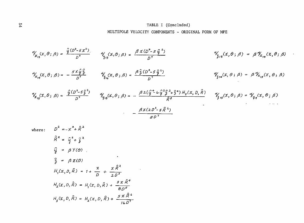
TABLE I (Concluded)
MULTIPOLE VELOCITY COMPONENTS - ORIGINAL FORM OF MPE
%4(Z1&
0~z,; 1)
-
(%
X,)-_
pzq49a;4)
2'
z v7 U /9,
P
=h 13 1(Z 19;)
where : D = %=+1?
80'
9= =
2~
whre,:
fl y(&)
,Sz09) XD
= ,
;z
x,,)+
R^ 92 2
4/
,
887
Z D7
D,/zD,,? L 3 z
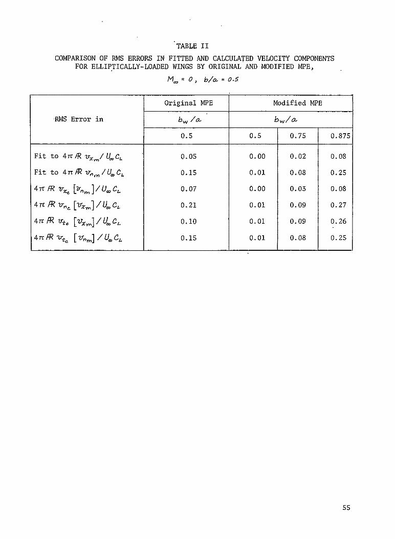
TABLE II
COMPARISON OF RMS ERRORS IN FITTED AND CALCULATED VELOCITY COMPONENTS FOR ELLIPTICALLY-LOADED WINGS BY ORIGINAL AND MODIFIED MPE,
mt = 0, b/o= 0.5
-RMS Error in
Fit to 4 TrR -v/t,/ C1
Fit to 4n/R v,, /UJ C1
47R 'r., [.]/u4c
4Trh v. [-v,]/U 0C,
4 rr ut, [u,] /U. CL
4 TrR . [zv, ]/u.
Original MPE
b w /0-
0.5
0.05
0.15
0.07
0.21
0.10
0.1S
0.5
0.00
0.01
0.00
0.01
0.01
0.01
Modified MPE
b,10,
0.75 0.875
0.02 0.08
0.08 0.25
0.03 0.08
0.09 0.27
0.09 0.26
0.08 0.25
55
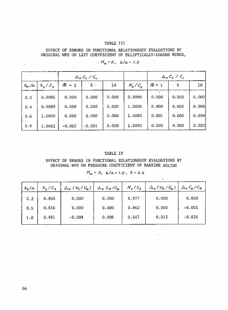
TABLE III
EFFECT OF ERRORS IN FUNCTIONAL RELATIONSHIP EVALUATIONS BY ORIGINAL MPE ON LIFT COEFFICIENT OF ELLIPTICALLY-LOADED WINGS,
.M, =O, b/a.= 1.0
R =N/C2b, lo. X2 /C 2 A=i 5. 10 1 5 10
0.2 0.9986 0.000 0.000 0.000 0.9986 0.000 0.000 0.000
0.4 0.9989 0.000 0.000 0.000 1.0006 0.000 0.000 0.000
0.6 1.0009 0.000 0.000 0.000 1.0080 0.001 0.000 0.000
0.8 1.0062 -0.002 -0.001 0.000 1.0285 0.009 0.003 0.002
TABLE IV
EFFECT OF ERRORS IN FUNCTIONAL RELATIONSHIP EVALUATIONS BY
ORIGINAL MPE ON PRESSURE COEFFICIENT OF RANKINE SOLIDS
M = 0, b/a = 0=.1.o0, z
bb /a. X 3 /C3 A%(zrx/U&) Azc-P/Co /9,/C 3 A~Qx/ 0 AC/C
0.2 0.965 0.000 0.000 0.977 0.000 0.000
0.S 0.816 0.000 0.000 0.862 0.000 -0.001
1.0 0.481 -0.004 0.008 0.547 0.013 -0.026
56
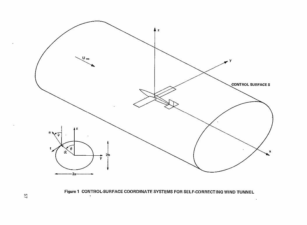
A z 0
COTOSURFACES
nv tz
,- ---- 2a ---I'-
Figure 1 CONTROL-SURFACE COORDINATE SYSTEMS FOR SELF-CORRECTING WIND TUNNEL
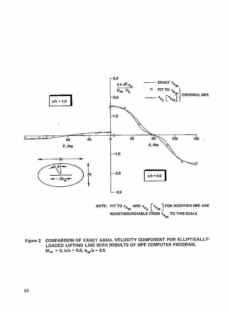
3.0
4 VR EXACTvx
U L0Trv m ORIGINAL MPE
Odeg0, dog
-t
-2.0
-3.0
NOTE: FIT TOVxm AND Vxc [Vnm] FOR MODIFIED MPE ARE
INDISTINGUISHABLE FROM TO THIS SCALE
Figure 2 COMPARISON OF EXACT AXIAL VELOCITY COMPONENT FOR ELLIPTICALLY-
LOADED LIFTING LINE WITH RESULTS OF MPE COMPUTER PROGRAM, Moo = 0, b/a = 0.5, bw/a = 0.5
58

3.0 EXACT Vnm,
4r-Rv 0 FITTO nm
-U_LtitLJ
C
2.00Ln $ORIGINAL MPE
180, 135 90 415
• " 2a
-3.0
NOTE: FIT TO Vnm AND vnc Vxm] FOR MODIFIED MPE ARE
INDISTINGUISHABLE FROM vnm TO THIS SCALE
Figure 3 COMPARISON OF EXACT NORMAL VELOCITY COMPONENT FOR ELLIPTICALLY-LOADED LIFTING LINE WITH RESULTS OF MPE COMPUTER PROGRAM, M o = 0, b/a = 0.5, bw/a = 0.5
59

-15 x 10 3
IEXACT Vxm
lOx a FIT TO Vxm
-5x 10⁻³
-3 -2 2 3
01
--5 x 10'3
Figure 4 COMPARISON OF EXACT AXIAL VELOCITY COMPONENT FOR RANKINE SOLID WITH RESULTS OF ORIGINIAL MPE COMPUTER PROGRAM, Mc,=O, b/a = 1.0, bb/a = 1.0,T= 0.2, e = 0
60

30 xl0Y EXACT v
03 FIT TO vn mm
91 VnclL[Vxmm
-5 x 10'3
/ / Vn/Uo
/
/0ITI
-4 -3 -2 -1 0 1 4 3-.. .. 4
/
/ /
x 10-3-10
Figure 5 COMPARISON OF EXACT NORMAL VELOCITY COMPONENT FOR RANKINE SOLID WITH RESULTS OF ORIGINAL MPE COMPUTER PROGRAM, Mo = 0, b/a = T0, bb/a = 1.0, T = 0.2, E = 0
61

4.0
-3.x47rA.i-47rA V
-2.0
- 0,,
\x
--0
EXACT Vxm -FITTO vxm
Vx.[Vn
-1.0
180I 1k 0
0, deg
45 0 d5 15135 0, deg
- 18180
--2.0 I/co
3.0
--4.0
Figure 6 COMPARISON OF EXACT AXIAL VELOCITY COMPONENT FOR ELLIPTICALLY-LOADED LIFTING LINE WITH RESULTS OF MODIFIED MPE COMPUTER PROGRAM, M. = 0, b/a = 0.5, bw/a = 0.875
62

5.0
0o ., EXACT
° -4.0 0 FIT TO vnm
4rA v l- nm Um CL
-3.0
-2.0
-1.0 I
I 0I/ I
180 135 045 45 135 180 0,deg / 9,deg
-1.0
I I
I - 3.
- 4.0
k I\ I
- 5.0
Figure 7 COMPARISON OF EXACT NORMAL VELOCITY COMPONENT FOR ELLIPTICALLY-LOADED LIFTING LINE WITH RESULTS OF MODIFIED MPE COMPUTER PROGRAM, M m = 0, b/a = 0.5, bw/a = 0.875
63

34- EXACT Vxm 4rV 0 -FITTOv
2.0 CL x [vam
90 4510 5900 135 1 0
,deg 0,d: -1I.0 "-"
-- 2.0 0
-- 3.0
Figure 8 COMPARISON OF EXACT AXIAL VELOCITY COMPONENT FOR ELLIPTICALLY-LOADED LIFTING LINE WITH RESULTS OF MODIFIED MPE COMPUTER PROGRAM,
IFTING LINE OFFSET FROM MPE ORIGIN BY xo/a = 0.25, M.= 0, b/a = 0.5,
N/a = 0.5
64
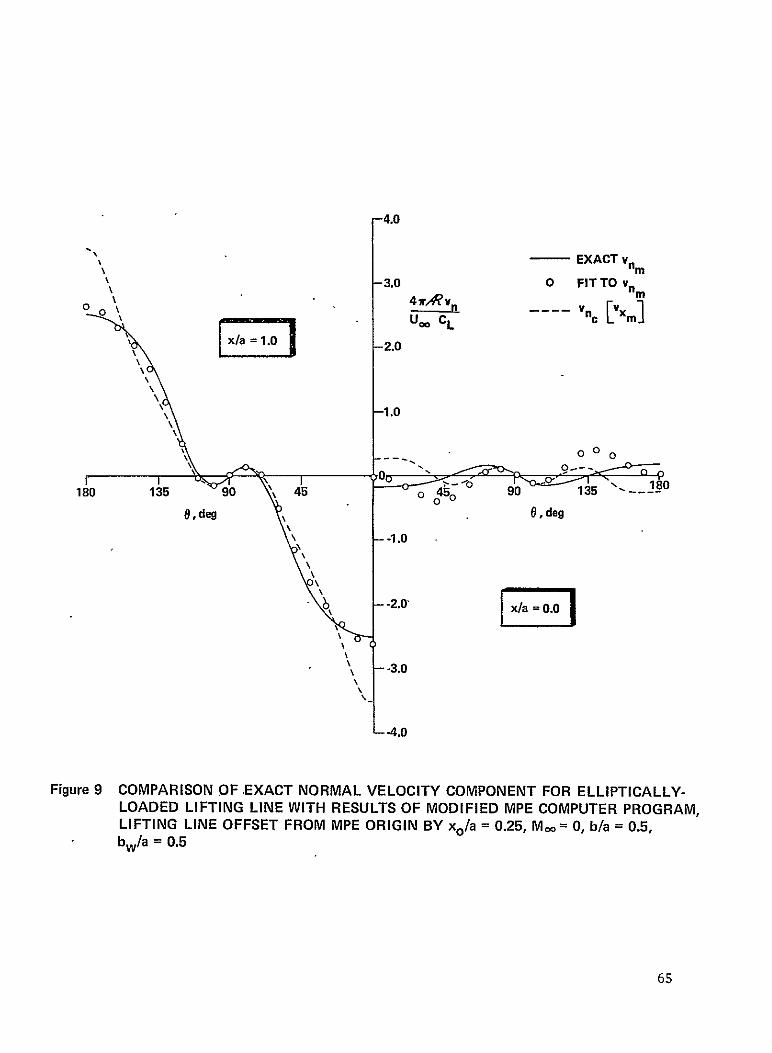
4.0
\ EXACT Vnm
-3.0 0 FIT TO vn,0 o\ - .n n .
Ix~a=1.OI2.0 l \\ ,.-1.0
___ . o 00
45 45 ~ 1180 135 90 \ 0o 40 90U 8, deg 0\, deg
• \\\\\\--1.0
• - ~-2.0' x/ = O
\S \ - -3.0
--4.0
Figure 9 COMPARISON OF EXACT NORMAL VELOCITY COMPONENT FOR ELLIPTICALLY-LOADED LIFTING LINE WITH RESULTS OF MODIFIED MPE COMPUTER PROGRAM,
=LIFTING LINE OFFSET FROM MPE ORIGIN BY xo/a = 0.25, M.& 0, b/a = 0.5, bw/a = 0.5
65

.0
0 - EXACT Vxm
4.0 0 FIT TO vx
---- Xm4 .... Vxc Enm]
x -3c.0 vx
L 3.0 \
00
.2.0
-1.0 0
\
0 ----T 45 0 45135 180
6 ,deg 0,deg-0 , , ' '
-1.00
-c-----2a-
--3.0
Figure 10 COMPARISON OF EXACT AXIAL VELOCITY COMPONENT FOR ELLIPTICALLY-
LOADED LIFTING LINE WITH RESULTS OF MODIFIED MPE COMPUTER PROGRAM, =LIFTING LINE OFFSET FROM MPE ORIGIN BY zo/a 0.25, M= 0, b/a = 0.5,
bw/a = 0.5
66

3.0 - EXACT vnm
10 4 vn 0 FIT TO vnmU 0mCL Vn [ ,o , -2.90.. 1 18E 9
\ -1.0 \
0 0
\/a0 , 0.5 180 135 90 0450 90 13586
8, dog -4. 6, deg
\0
--1.0 1
LITN IEOFE FO \zP --RGNB3.01" z .5 ~ /a 0.5
t 2b \w
--!0
--5.0
Figure 11 COMPARISON OF EXACT NORMAL VELOCITY COMPONENT FOR ELLIPTICALLY-LOADED LIFTING LINE WITH RESULTS OF MODIFIED MPE COMPUTER PROGRAM, LIFTING LINE OFFSET FROM MPE ORIGIN BY zo/a = 0.25, M.o = 0, b/a = 0.5, bw/a = 0.5
67

3.0. EXACT vxm
r- y0 FIT TO Vxm
Uo 2.0 c ln]1CL
-1.0
- 0
45 45 135 180180 135 0
0, deg0 ,deg
-- 2.04 2 2 "
2b -3.0
h\
yy7yyyy/ y77yyyy 7,7y7y77 -4.0
- 5.0
Figure 12 COMPARISON OF EXACT AXIAL VELOCITY COMPONENT FOR ELLIPTICALLY-LOADED LIFTING LINE IN GROUND EFFECT WITH RESULTS OF MODIFIED
= MPE COMPUTER PROGRAM, M. = 0, b/a = 0.5, bw/a = 0.75, hg/bw 0.8
68

-3.0- EXACT Vnm 4 ,v 0 FIT TOyn
Um C,_-2.0 0
. .- o [Vx ]MI
\I 1.0I 0
II
00
180 135 90 45 0 45 90 135 180
0, deg IO,deg ~---1.0
-'-2.0
-- 3.0-a 2b- -2
,///.x777, -- 4.0
Figure 13 COMPARISON OF EXACT NORMAL VELOCITY COMPONENT FOR ELLIPTICALLY-LOADED LIFTING LINE IN GROUND.EFFECT WITH RESULTS OF MODIFIED MPE
0 7 5 COMPUTER PROGRAM, M00. = 0, b/a = 0.5, bw/a = . , hg/bw = 0.8
69
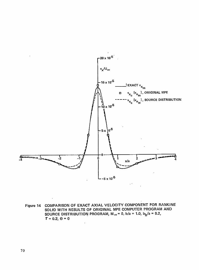
4
vx/Uoo
15 x 105
____I EXACT Vxm
1\o] VXC [Vnm], ORIGINAL MPE
.. Vxc [Vnm ], SOURCE DISTRIBUTION ,-lx 10'5
-5 x10⁻⁵
3 _3 --2 -- ,o x/a4-4I/\
--5 X 10'5
Figure 14 COMPARISON OF EXACT AXIAL VELOCITY COMPONENT FOR RANKINE
SOLID WITH RESULTS OF ORIGINAL MIPE COMPUTER PROGRAM AND = 1-0, bb/a = 0.2,SOURCE DISTRIBUTION PROGRAM, M.o= 0, b/a
7T= 0.2, E= 0
70

SURFACE S
t
(a) VEHICLE IN FLIGHT
Figure 15 DEFINITION OF INTERIOR (I) AND EXTERIOR (I) REGIONS IN UNCONFINED FLOW ABOUT A VTOL CONFIGURATION
71

SURFACE S
U00
(b) FLOW IN REGIONIT
Figure 15 (Continued) DEFINITION OF INTERIOR (I) AND EXTERIOR (II) REGIONS IN
UNCONFINED FLOW ABOUT A VTOL CONFIGURATION
72

SURFACES z
h
V
U0 v
h
"3T SURFACE S
Figure 16 UNCONFINED TWO-DIMENSIONAL FLOW ABOUT AN AIRFOIL

ADJUST: FLOWAT CONTROL MEASURE DISTURBANCE VELOCITIES
MODEL ATTITUDE TIVE USE OF WALLS AT CONTROL SURFACEIvzm vxm COMPUTE: OUTER FLOW FIELD
AND DETERMINE vzc
AT CQNTROL SURFACEo'm vz°
MEASURE:' MODEL FORCES. MOMENTS, PRESSURES, ETC.
Figure 17 SELF-CORRECTING WIND TUNNEL SCHEME