Embed Size (px)
Citation preview
CPU Scheduling
Operating Systems: Internals and Design Principles, 6/E
William StallingsOperating System Concept : Silberschatz, Galvin and Gagne
Dave BremerOtago Polytechnic, N.Z.
©2008, Prentice Hall
Dr. Sunny Jeong & Mr. M.H. Park
CPU Scheduling
• Basic Concepts
• Scheduling Criteria
• Scheduling Algorithms
• Thread Scheduling
• Multiple-Processor Scheduling
• Algorithm Evaluation
Objectives
• To introduce CPU scheduling, which is the basis for multiprogrammed operating systems
• To describe various CPU-scheduling algorithms
• To discuss evaluation criteria for selecting a CPU-scheduling algorithm for a particular system
Basic Concepts
• Maximum CPU utilization obtained with multiprogramming
• CPU–I/O Burst Cycle – Process execution consists of a cycle of CPU execution and I/O wait
• CPU burst distribution
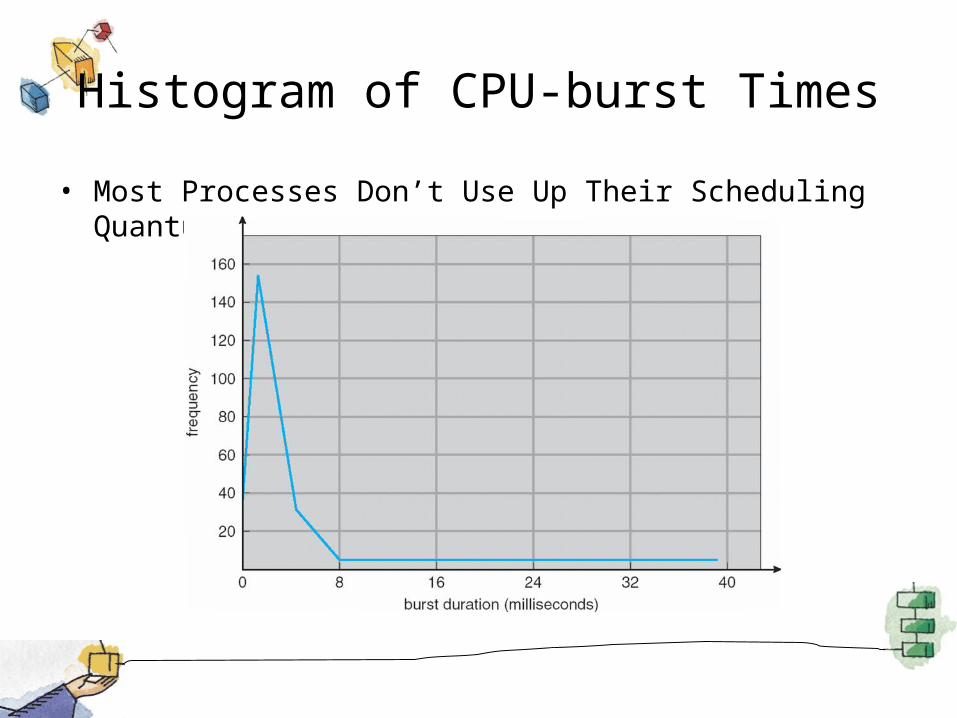
Histogram of CPU-burst Times
• Most Processes Don’t Use Up Their Scheduling Quantum!
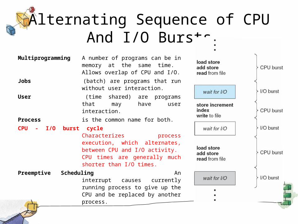
Alternating Sequence of CPU And I/O Bursts
Multiprogramming A number of programs can be in memory at the same time. Allows overlap of CPU and I/O.
Jobs (batch) are programs that run without user interaction.
User (time shared) are programs that may have user interaction.
Process is the common name for both.
CPU - I/O burst cycle Characterizes process execution, which alternates, between CPU and I/O activity. CPU times are generally much shorter than I/O times.
Preemptive Scheduling An interrupt causes currently running process to give up the CPU and be replaced by another process.
CPU Scheduler
• Selects from among the processes in memory that are ready to execute, and allocates the CPU to one of them
• CPU scheduling decisions may take place when a process:1. Switches from running to waiting state
2. Switches from running to ready state
3. Switches from waiting to ready
4. Terminates
• Scheduling under 1 and 4 is nonpreemptive
• All other scheduling is preemptive
Dispatcher
• Dispatcher module gives control of the CPU to the process selected by the short-term scheduler; this involves:– switching context– switching to user mode– jumping to the proper location in the user program to
restart that program
• Dispatch latency – time it takes for the dispatcher to stop one process and start another running
Scheduling Criteria
• CPU utilization – keep the CPU as busy as possible
• Throughput – # of processes that complete their execution per time unit
• Turnaround time – amount of time to execute a particular process
• Waiting time – amount of time a process has been waiting in the ready queue
• Response time – amount of time it takes from when a request was submitted until the first response is produced, not output (for time-sharing environment)
Scheduling Algorithm Optimization Criteria
• Max CPU utilization
• Max throughput
• Min turnaround time
• Min waiting time
• Min response time
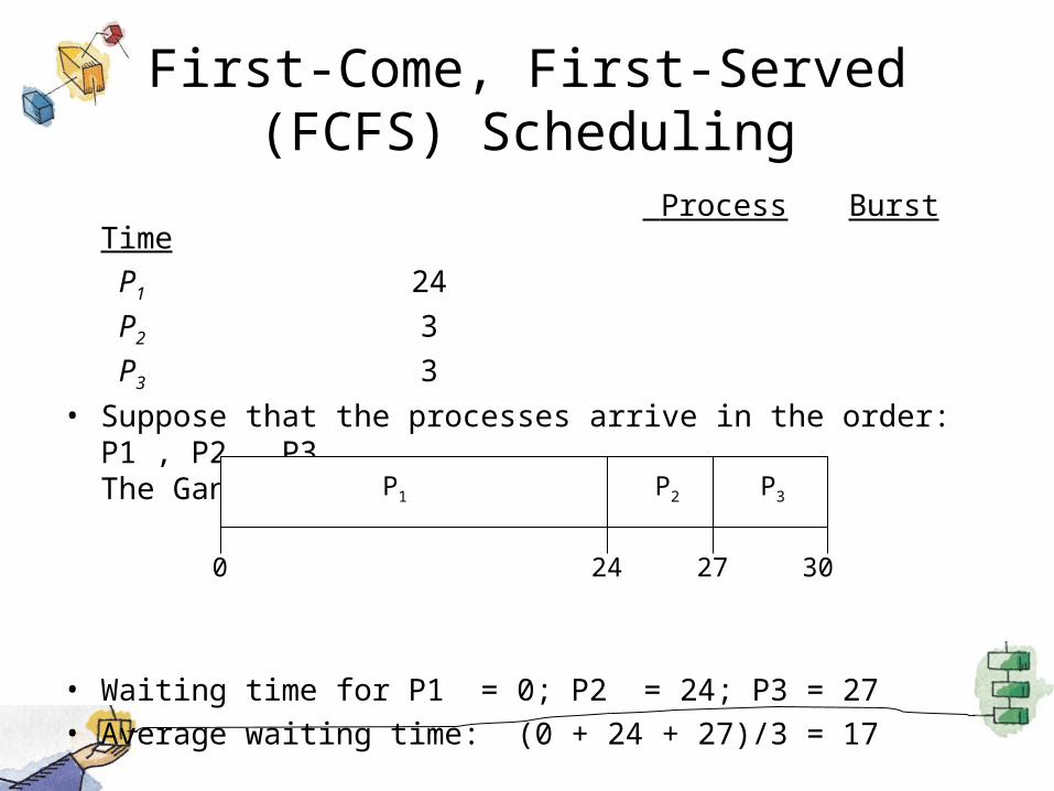
First-Come, First-Served (FCFS) Scheduling
Process Burst Time
P1 24
P2 3
P3 3
• Suppose that the processes arrive in the order: P1 , P2 , P3 The Gantt Chart for the schedule is:
• Waiting time for P1 = 0; P2 = 24; P3 = 27
• Average waiting time: (0 + 24 + 27)/3 = 17
P1 P2 P3
24 27 300
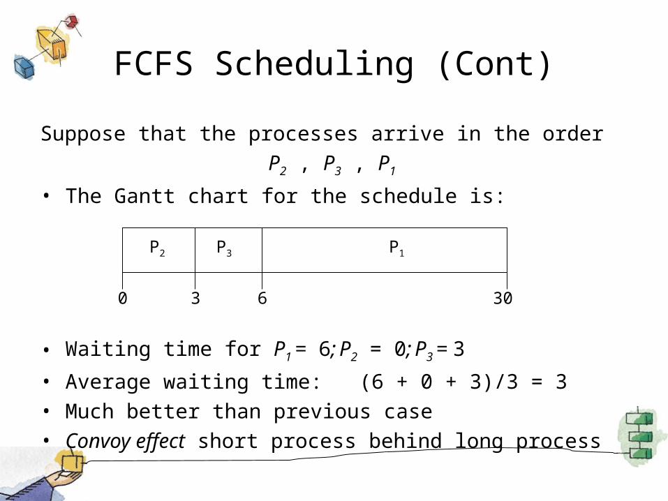
FCFS Scheduling (Cont)
Suppose that the processes arrive in the order
P2 , P3 , P1
• The Gantt chart for the schedule is:
• Waiting time for P1 = 6; P2 = 0; P3 = 3
• Average waiting time: (6 + 0 + 3)/3 = 3
• Much better than previous case
• Convoy effect short process behind long process
P1P3P2
63 300
Shortest-Job-First (SJF) Scheduling
• Associate with each process the length of its next CPU burst. Use these lengths to schedule the process with the shortest time
• SJF is optimal – gives minimum average waiting time for a given set of processes– The difficulty is knowing the length of the next CPU request
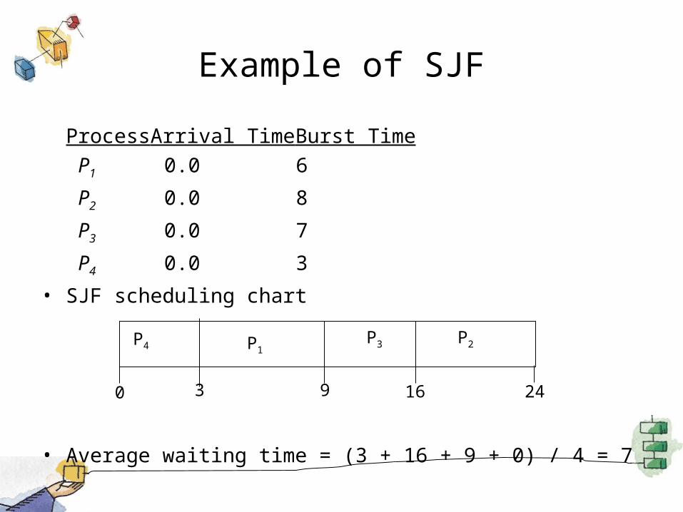
Example of SJF
Process Arrival Time Burst Time
P1 0.0 6
P2 0.0 8
P3 0.0 7
P4 0.0 3
• SJF scheduling chart
• Average waiting time = (3 + 16 + 9 + 0) / 4 = 7
P4P3P1
3 160 9
P2
24
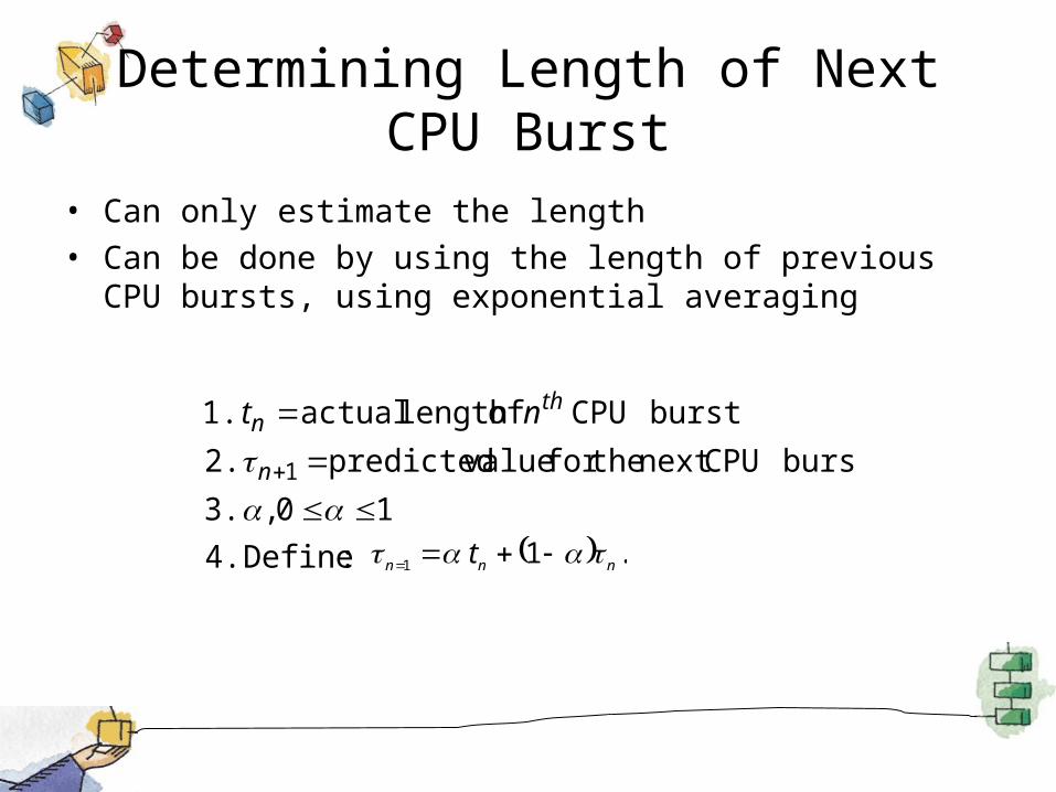
Determining Length of Next CPU Burst
• Can only estimate the length
• Can be done by using the length of previous CPU bursts, using exponential averaging
:Define 4.
10 , 3.
burst CPU next the for value predicted 2.
burst CPU of length actual 1.
1n
thn nt
.1 1 nnn t
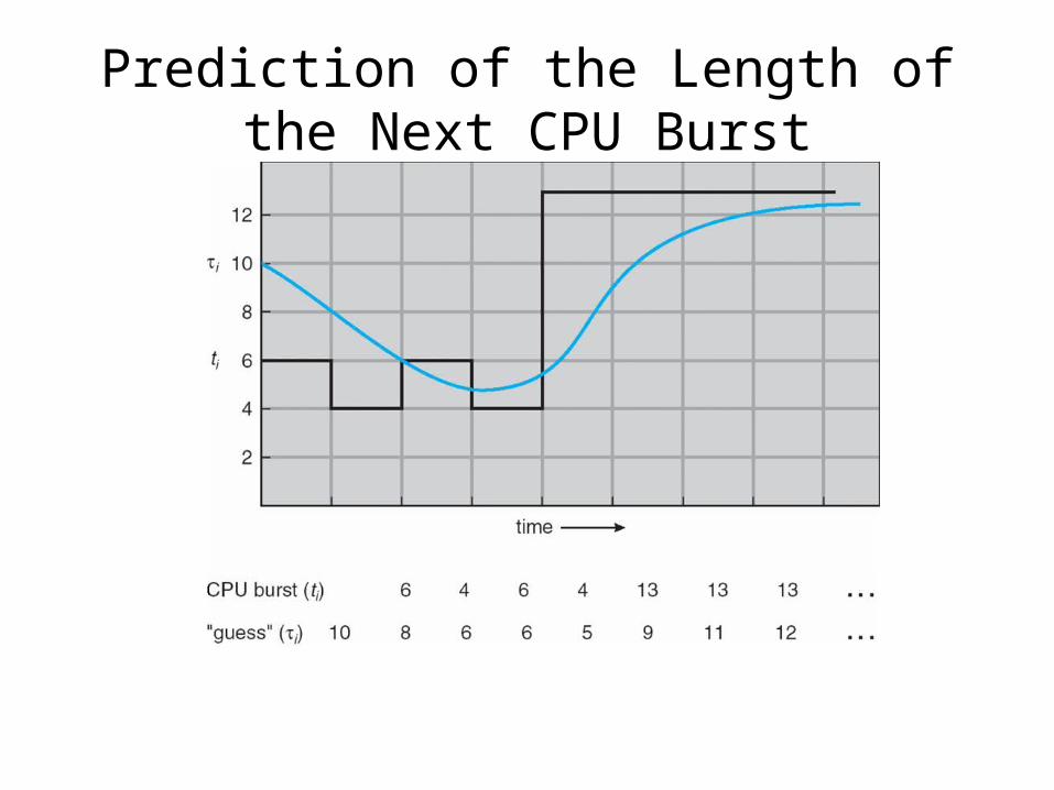
Prediction of the Length of the Next CPU Burst
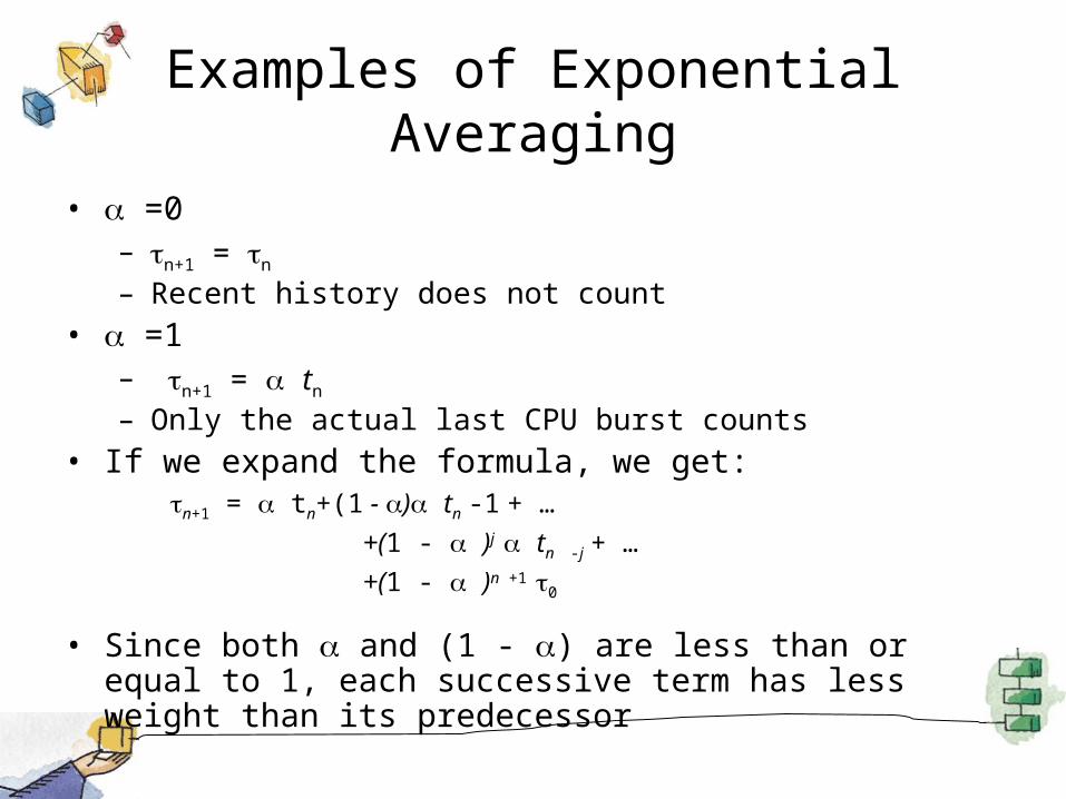
Examples of Exponential Averaging
• =0– n+1 = n
– Recent history does not count
• =1– n+1 = tn
– Only the actual last CPU burst counts
• If we expand the formula, we get:n+1 = tn+(1 - ) tn -1 + …
+(1 - )j tn -j + …
+(1 - )n +1 0
• Since both and (1 - ) are less than or equal to 1, each successive term has less weight than its predecessor
Priority Scheduling
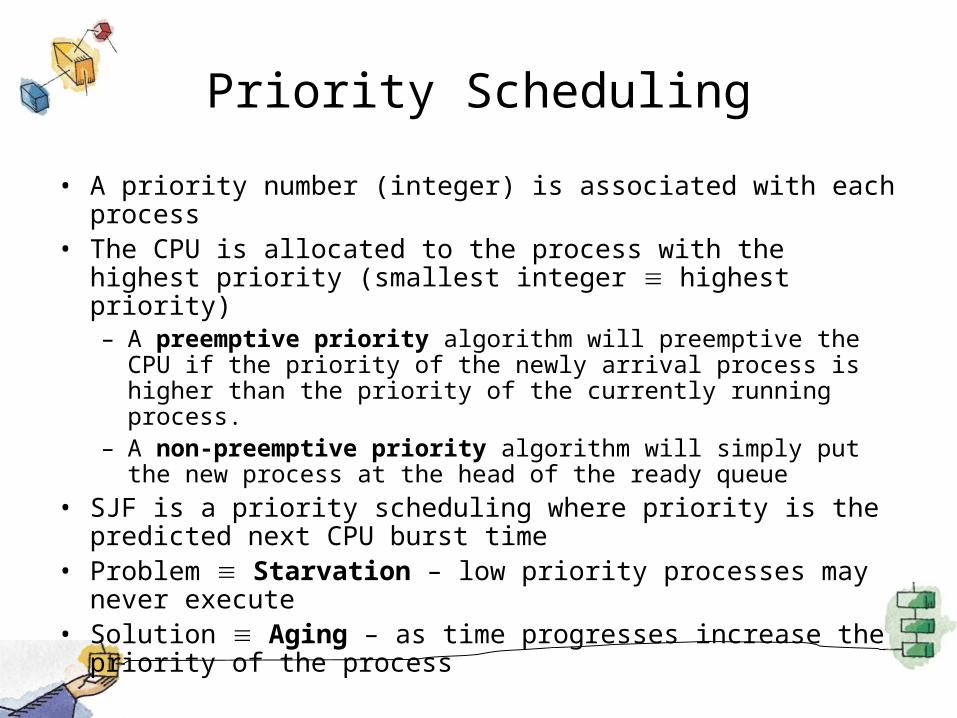
• A priority number (integer) is associated with each process• The CPU is allocated to the process with the highest priority
(smallest integer highest priority)– A preemptive priority algorithm will preemptive the CPU if the
priority of the newly arrival process is higher than the priority of the currently running process.
– A non-preemptive priority algorithm will simply put the new process at the head of the ready queue
• SJF is a priority scheduling where priority is the predicted next CPU burst time
• Problem Starvation – low priority processes may never execute
• Solution Aging – as time progresses increase the priority of the process
Round Robin (RR)
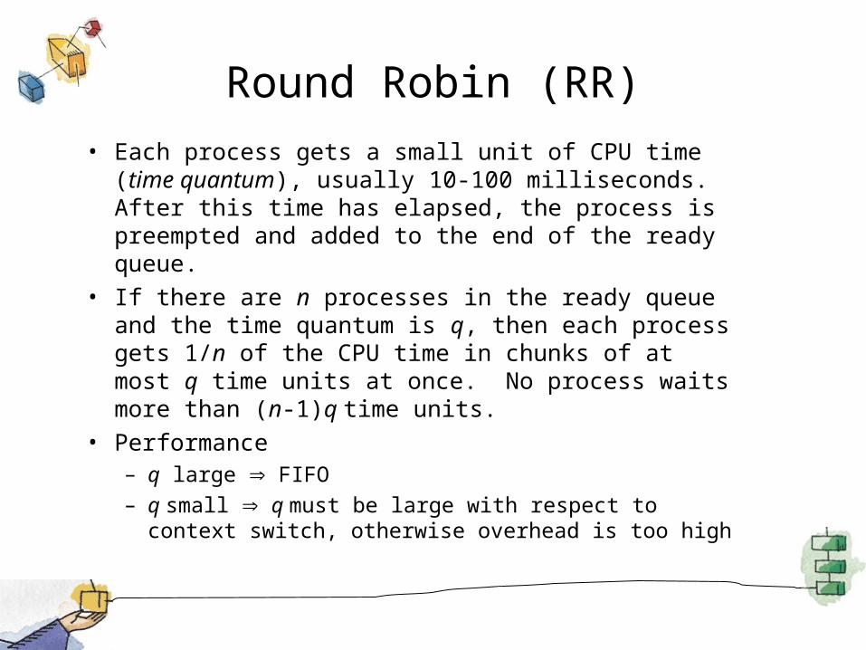
• Each process gets a small unit of CPU time (time quantum), usually 10-100 milliseconds. After this time has elapsed, the process is preempted and added to the end of the ready queue.
• If there are n processes in the ready queue and the time quantum is q, then each process gets 1/n of the CPU time in chunks of at most q time units at once. No process waits more than (n-1)q time units.
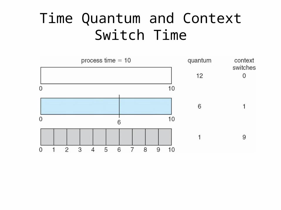
• Performance– q large FIFO– q small q must be large with respect to context
switch, otherwise overhead is too high
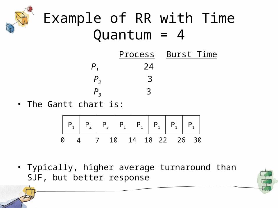
Example of RR with Time Quantum = 4
Process Burst Time
P1 24
P2 3
P3 3
• The Gantt chart is:
• Typically, higher average turnaround than SJF, but better response
P1 P2 P3 P1 P1 P1 P1 P1
0 4 7 10 14 18 22 26 30
Time Quantum and Context Switch Time
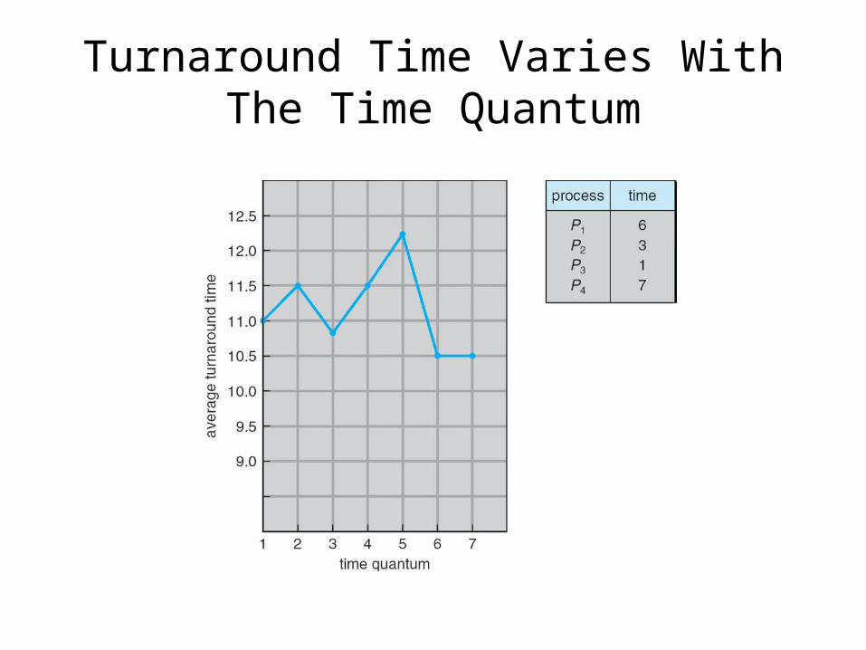
Turnaround Time Varies With The Time Quantum
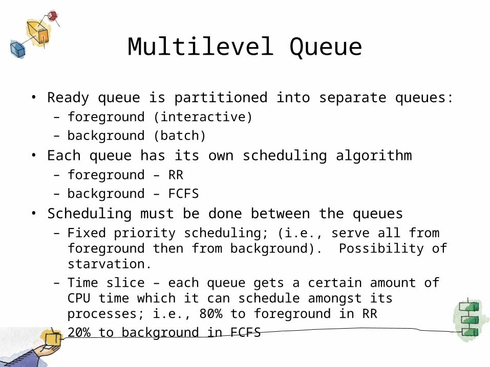
Multilevel Queue
• Ready queue is partitioned into separate queues:– foreground (interactive)– background (batch)
• Each queue has its own scheduling algorithm– foreground – RR– background – FCFS
• Scheduling must be done between the queues– Fixed priority scheduling; (i.e., serve all from foreground then
from background). Possibility of starvation.– Time slice – each queue gets a certain amount of CPU time
which it can schedule amongst its processes; i.e., 80% to foreground in RR
– 20% to background in FCFS
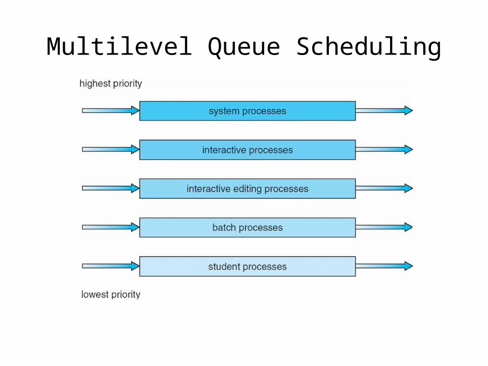
Multilevel Queue Scheduling
Multilevel Feedback Queue
• A process can move between the various queues; aging can be implemented this way
• Multilevel-feedback-queue scheduler defined by the following parameters:– number of queues– scheduling algorithms for each queue– method used to determine when to upgrade a process– method used to determine when to demote a process– method used to determine which queue a process will enter
when that process needs service
Example of Multilevel Feedback Queue
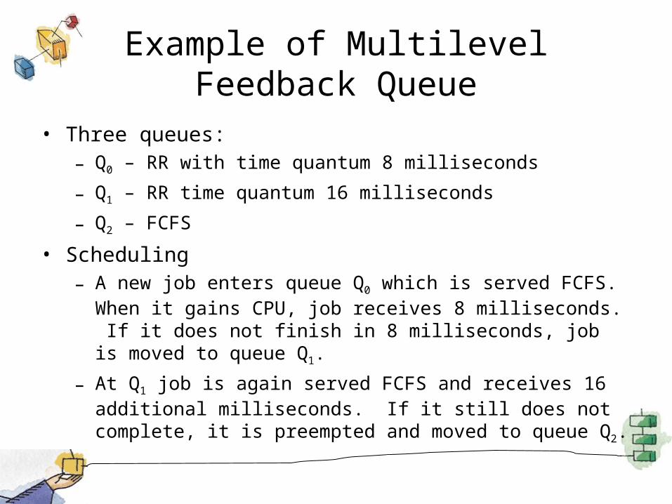
• Three queues: – Q0 – RR with time quantum 8 milliseconds
– Q1 – RR time quantum 16 milliseconds
– Q2 – FCFS
• Scheduling– A new job enters queue Q0 which is served FCFS. When it gains
CPU, job receives 8 milliseconds. If it does not finish in 8 milliseconds, job is moved to queue Q1.
– At Q1 job is again served FCFS and receives 16 additional milliseconds. If it still does not complete, it is preempted and moved to queue Q2.
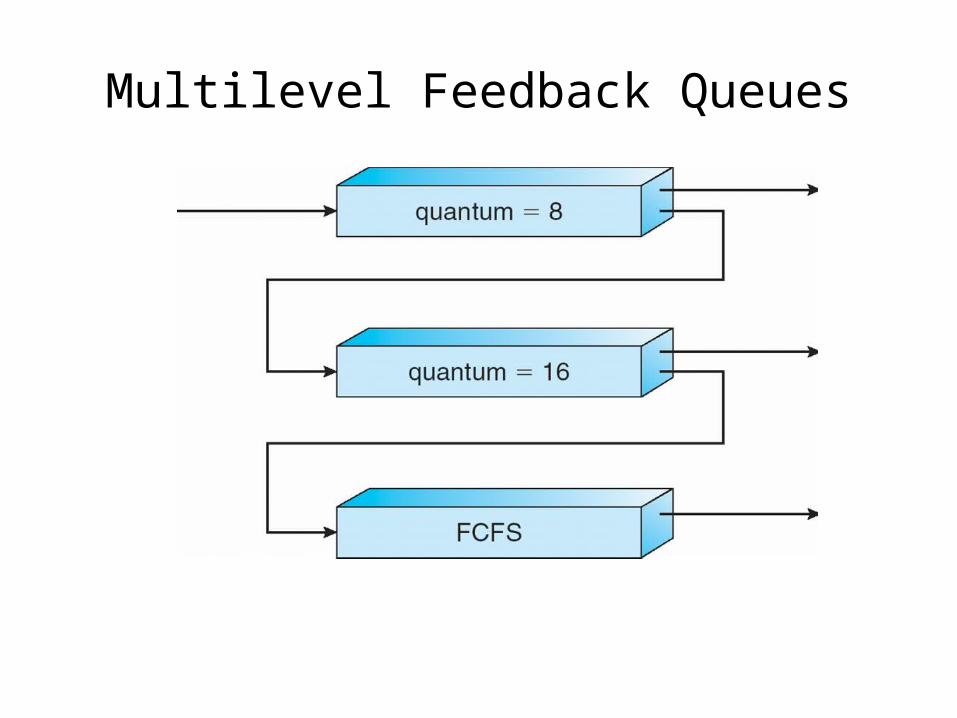
Multilevel Feedback Queues
Wrapup
• We’ve looked at a number of different scheduling algorithms.
• Which one works the best is application dependent.
– General purpose OS will use priority based, round robin, preemptive
– Real Time OS will use priority, no preemption.
Thread Scheduling
• Distinction between user-level and kernel-level threads
• Many-to-one and many-to-many models, thread library schedules user-level threads to run on LWP– Known as process-contention scope (PCS) since scheduling
competition is within the process
• Kernel thread scheduled onto available CPU is system-contention scope (SCS) – competition among all threads in system
Multiple-Processor Scheduling
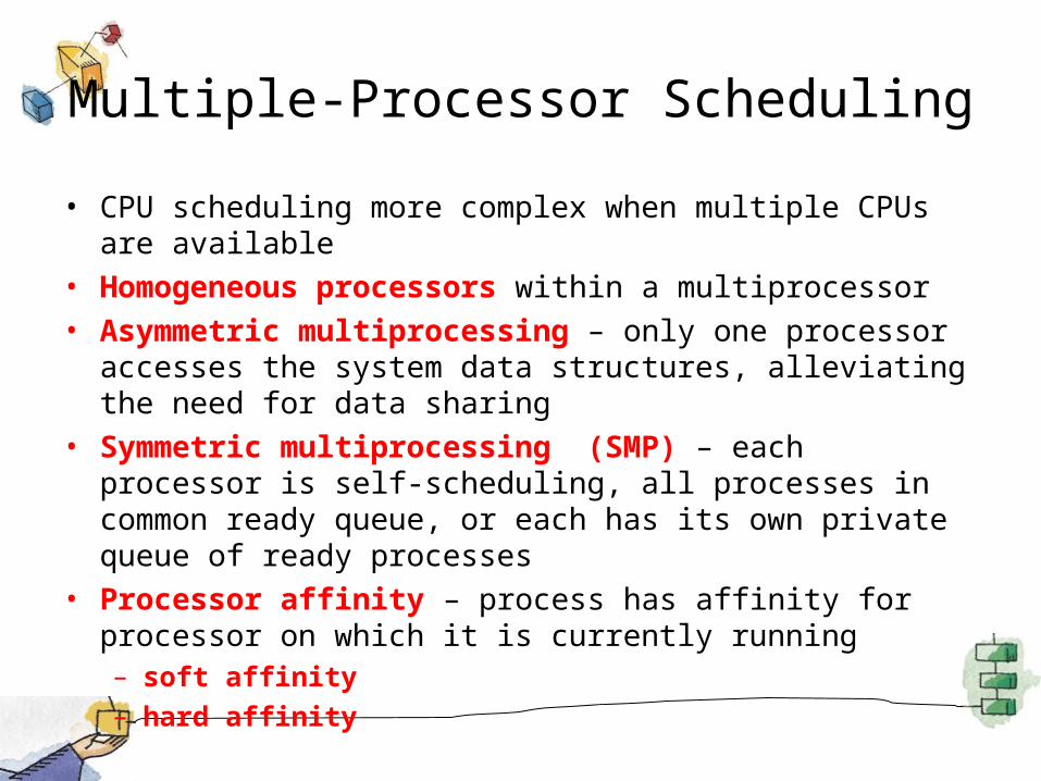
• CPU scheduling more complex when multiple CPUs are available
• Homogeneous processors within a multiprocessor
• Asymmetric multiprocessing – only one processor accesses the system data structures, alleviating the need for data sharing
• Symmetric multiprocessing (SMP) – each processor is self-scheduling, all processes in common ready queue, or each has its own private queue of ready processes
• Processor affinity – process has affinity for processor on which it is currently running– soft affinity– hard affinity
Multicore Processors
• Recent trend to place multiple processor cores on same physical chip
• Faster and consume less power
• Multiple threads per core also growing– Takes advantage of memory stall to make progress on another
thread while memory retrieve happens
Algorithm Evaluation
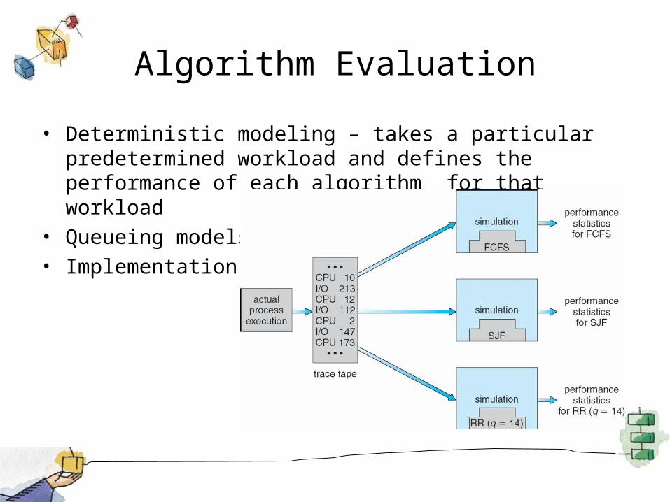
• Deterministic modeling – takes a particular predetermined workload and defines the performance of each algorithm for that workload
• Queueing models
• Implementation
Scheduling algorithm example
RR: Round Robin
Description
• The following Java program emulates the Round Robin scheduling method.
• It accepts process attributes and time slice. It then assigns time slices equally to all processes sequentially.
• Such kind of scheduling is used in CPUs to ensure that starvation does not happen.
• It is one of the most simplest type of scheduling.
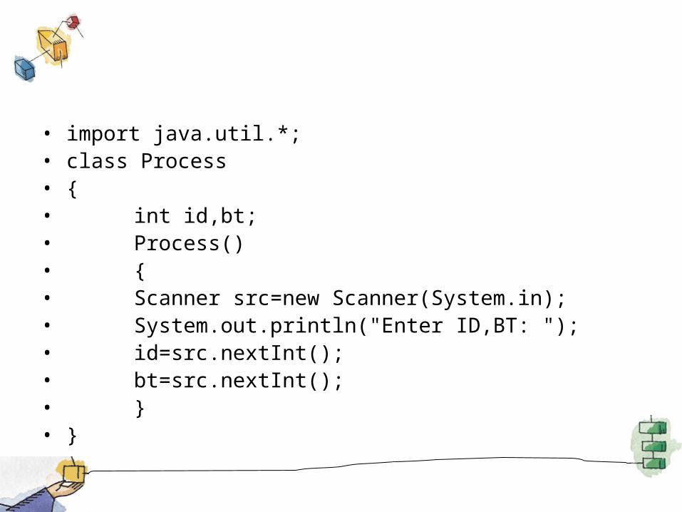
• import java.util.*;• class Process• {• int id,bt;• Process()• {• Scanner src=new Scanner(System.in);• System.out.println("Enter ID,BT: ");• id=src.nextInt();• bt=src.nextInt();• }• }
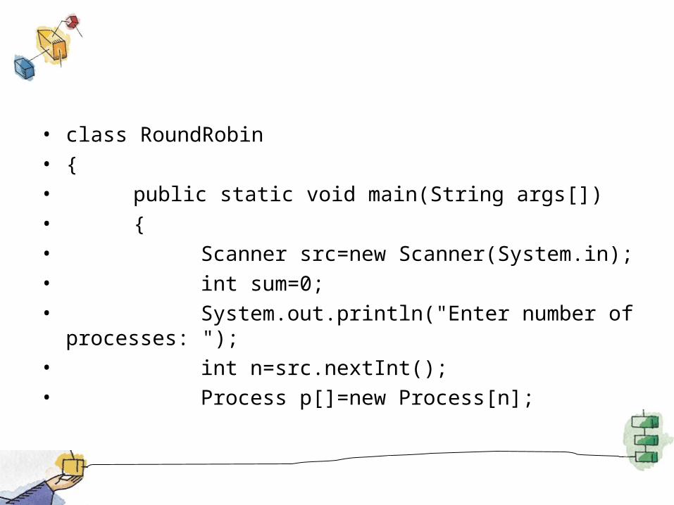
• class RoundRobin
• {
• public static void main(String args[])
• {
• Scanner src=new Scanner(System.in);
• int sum=0;
• System.out.println("Enter number of processes: ");
• int n=src.nextInt();
• Process p[]=new Process[n];
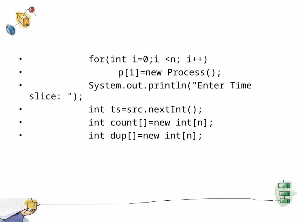
• for(int i=0;i <n; i++)
• p[i]=new Process();
• System.out.println("Enter Time slice: ");
• int ts=src.nextInt();
• int count[]=new int[n];
• int dup[]=new int[n];
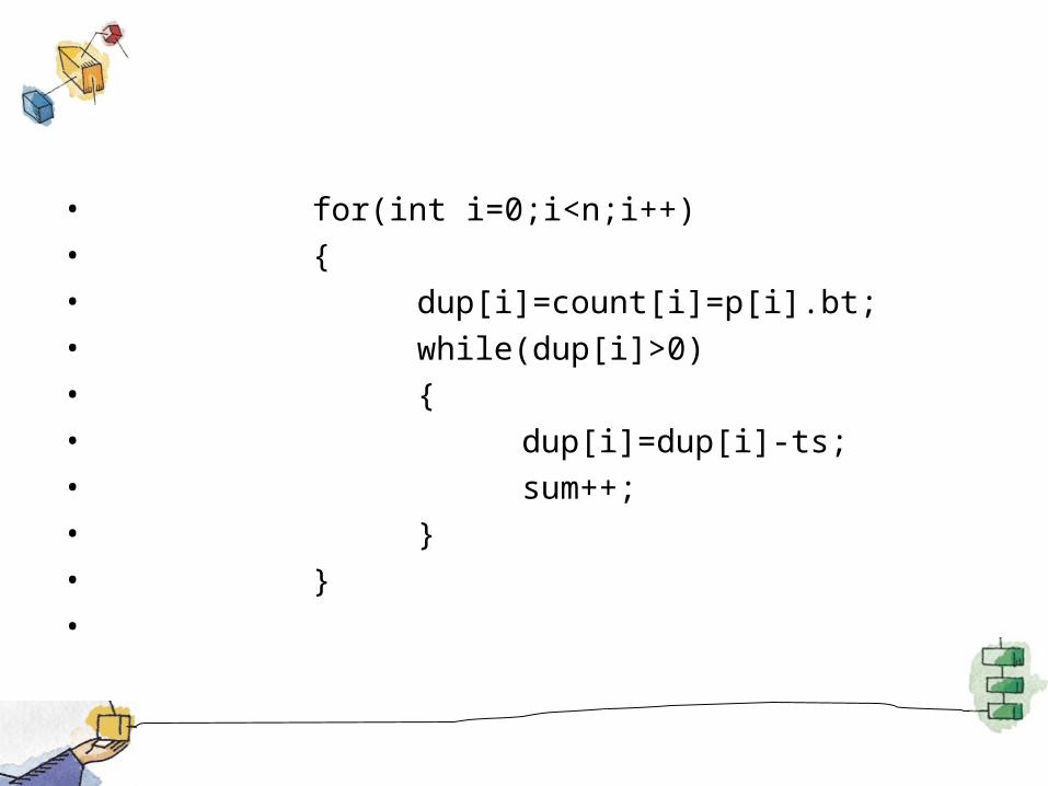
• for(int i=0;i<n;i++)
• {
• dup[i]=count[i]=p[i].bt;
• while(dup[i]>0)
• {
• dup[i]=dup[i]-ts;
• sum++;
• }
• }
•
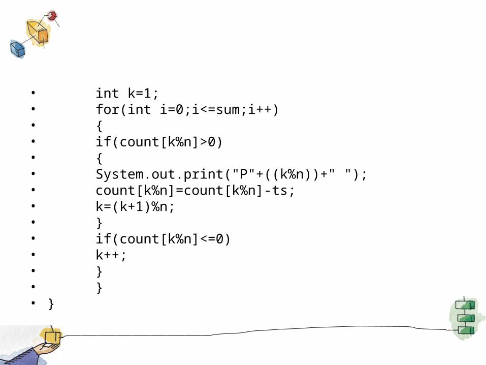
• int k=1;• for(int i=0;i<=sum;i++)• {• if(count[k%n]>0)• {• System.out.print("P"+((k%n))+" ");• count[k%n]=count[k%n]-ts;• k=(k+1)%n;• }• if(count[k%n]<=0)• k++;• }• }• }