CPIB SUMMER SCHOOL 2014: INTRODUCTION TO BIOLOGICAL MODELLINGnick-monk.staff.shef.ac.uk/CPIB-Summer-School/lect1p1_slides_2014.pdf · Summer School: Mathematical Modelling for Biologists!

July 2014 Summer School: Mathematical Modelling for Biologists

CPIB SUMMER SCHOOL 2014: INTRODUCTION TO BIOLOGICAL

MODELLING

University of Nottingham 14–17 July 2014


Aims: • To introduce modelling and quantitative approaches to biology • To explain where equations come from and what they mean, placing the

mathematics into a context that is relevant for the life scientist. • To enable life scientists to gain a better understanding of what a model is,

and how to go about building one.

Objectives: By the end of the session, participants will: • understand key concepts in how to build models of biological systems • know how to investigate the behaviour of those models • be able to interpret the results of those models.

Course Outline


The kinds of behaviour that dynamic models can exhibit (e.g. exponential growth or decay, steady states, oscillations, patterns), and their stability.

Single variable differential equation models: • How to work out their dynamics by sketching one simple graph. • Applications, including to population growth and gene regulation.

Multi-variable differential equation models: • Interacting populations, signalling networks, biochemical reactions. • How to turn reactions into a model with the law of mass action. • How to work out a lot about their dynamics by sketching two (or

more) graphs.

Parameter estimation and sensitivity

Including randomness - stochastic models

Spatial models - signalling, transport, growth and pattern formation

How to create, simulate and analyse models using appropriate software

Key Themes

Lecture 1.1��Mathematical modelling and Systems Biology


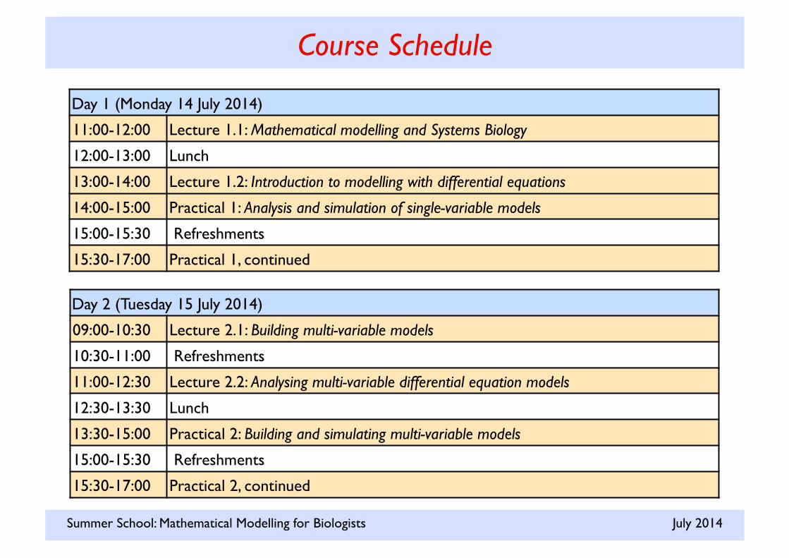
Day 1 (Monday 14 July 2014)

11:00-12:00 Lecture 1.1: Mathematical modelling and Systems Biology

12:00-13:00 Lunch

13:00-14:00 Lecture 1.2: Introduction to modelling with differential equations

14:00-15:00 Practical 1: Analysis and simulation of single-variable models

15:00-15:30 Refreshments

15:30-17:00 Practical 1, continued

Day 2 (Tuesday 15 July 2014)

09:00-10:30 Lecture 2.1: Building multi-variable models


11:00-12:30 Lecture 2.2: Analysing multi-variable differential equation models

12:30-13:30 Lunch

13:30-15:00 Practical 2: Building and simulating multi-variable models



Course Schedule


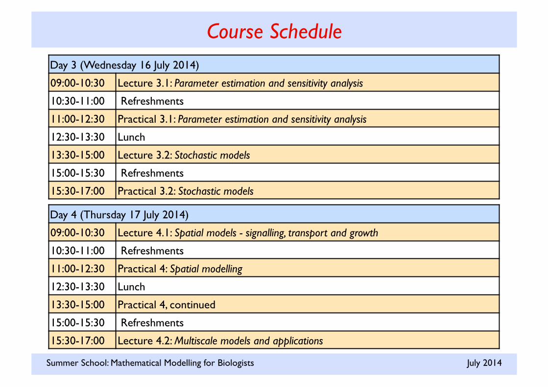
Day 4 (Thursday 17 July 2014)

09:00-10:30 Lecture 4.1: Spatial models - signalling, transport and growth


11:00-12:30 Practical 4: Spatial modelling

12:30-13:30 Lunch



15:30-17:00 Lecture 4.2: Multiscale models and applications

Course Schedule Day 3 (Wednesday 16 July 2014)

09:00-10:30 Lecture 3.1: Parameter estimation and sensitivity analysis


11:00-12:30 Practical 3.1: Parameter estimation and sensitivity analysis

12:30-13:30 Lunch

13:30-15:00 Lecture 3.2: Stochastic models


15:30-17:00 Practical 3.2: Stochastic models


What is Systems Biology?

" Biological systems: large numbers of components interacting at various scales. In the past, life scientists could only study a handful of components at a time. This often led to

an approach assuming a simple chain of cause and effect.Most genes, proteins, cells, organisms and other components work within a complex network of interactions, with

interlocking positive and negative feedback loops. Systems Biology provides a conceptual framework for understanding biological problems. It combines the mathematical,

computational, physical and engineering sciences with biological experiments.

The Biotechnology and Biosciences Research Council says:

“Systems biology is an approach by which biological questions are addressed through integrating experiments with computational modelling and theory, in re-enforcing cycles.”


What is Systems Biology?



Biological processes understood as emergent properties of complex networks of interacting components.

Question: what are the mechanisms regulating emergence?

Masamizu et al., PNAS. 2006

Hes1 (and other Notch pathway genes) oscillate in the presomitic mesoderm of developing vertebrate embryos.

Back to the beginning...


Inferring Networks

Components and interactions can be inferred from a wide range of data sources: • Genetic screens • RNAi screens • mRNA profiling (e.g. microarrays, NGS) • Metabolic profiling • Protein-protein interaction screens (e.g. yeast-two-hybrid, TAP mass spec.) • ChIP-on-chip analysis of transcription factor binding • Biochemistry • Population data (e.g. on predator-prey or epidemiological interactions)

Each has strengths and limitations; Integration of multiple data sources is important for reliable inference.


How to make a switch? Important for Cell differentiation, quorum sensing, lac operon inducible system, lysis-lysogeny decision by phage Lambda, ... Delta-Notch signalling is a simple example. Feedback + coupling selects a subpopulation of cells for a neuronal fate.

How to make an oscillator? Cell cycle, circadian rhythms, cardiac action-potential

How to make an organism? Fate determination + cell movements, proliferation, etc, etc, ...

Population growth and interactions From bacteria to humans; cancer (mutant cells invading a normal host); epidemiology; ecology; ...

What kinds of processes?


" Models help to encode our understanding and assumptions about a system " Can be used to test hypotheses, make predictions, carry out in silico experiments

(“What happens if ...?”) " Models are simplifications that can be extended when necessary (ideally in a loop

in association with experimental work).

Mathematical modelling approaches

" Compartmental models, e.g. ordinary differential equations

Rate of change of cancer volume = cell division cell ��

death killing via therapy - -

" Spatial models (e.g. partial differential equations, PDEs)

Rate of change of cancer cell

density = cell division cell

death killing via therapy - - + movement

" Individual-based models, e.g. cellular automaton

" Hybrid multiscale models - combining all of the above.


Variables, models and parameters • The system state is a set of measurable properties of the system. ��

Examples: mRNA & protein concentration, membrane potential, number of cells, …

• We would like to understand the past and present and predict the future. Given a set of measurements today, what will be the result of making those measurements tomorrow?

• A model is a representation of the system that we can use to answer such questions. ��If the state is changing with time (usually denoted t), then the model is dynamical. ��The time-varying components of the state are variables (e.g. denoted x1(t), x2(t), ..., xN(t)). The state of the model at time t is just the set of all the variables at time t:

S(t) = {x1(t), x2(t), ..., xN(t)}. • The form of model we shall study is:

S(t2) = f (S(t1); p1, p2, ..., pM), t2 > t1

where f is a function encoding our understanding of how the system components affect one another, and p1, p2, ..., pM are model parameters.This simply states that the future state of the system is some function of its past state ��(i.e. that the future is predictable).

• Parameters are numerical values that encode information about the system that is not included in the dynamic state. E.g. the concentration of an mRNA species is a variable; the linear degradation rate of the mRNA is a parameter.


• In reality, the state of each network component should be represented by a discrete quantity — an integer (e.g. the number of molecules of a particular mRNA in a cell, the number of individuals in a population).

• Also, changes in state over time are discrete events (production or degradation of a network component, births/deaths in a population).

• In practice, if the amount of each component is sufficiently large, then its state can be approximated by a continuous variable that changes smoothly and continuously in time (e.g. concentration, population density).

• In doing this, we are essentially representing a continuous process rather than a set of events.

Continuous Process Models


Ordinary differential equations (ODEs)

• If we represent the network state S(t) as continuous, then it has a well-defined rate of change:

• An ordinary differential equation (ODE) model gives the rates of change of the variables xi(t) as functions of the state at that time:

where <i> is the set of variables that affect xi(t). "• The functions fi encode the form of the interactions between components. These functions are hard to determine. There are no high-throughput methodologies for getting them.

• In practice, models are often based on a small set of standard representative forms for the fi (see later for examples). For chemical reactions, an important concept is the law of mass action..."

€

dxidt

t( ) = fi x i (t){ };p1, p2,…, pM( ), i =1,2,...,n€

dSdt

t( )


The law of Mass Action (1) • The law of mass action states that the rate of a chemical reaction is proportional to

the product of the concentrations of the reactants.

• Used to develop ODE models for networks of biochemical reactions.

• Assumptions: i) a well stirred solution and ii) low molecular concentrations, where the probability of diffusing molecules to get close enough, for a reaction to occur, is proportional to the concentrations.

• A rate parameter is used to define the ‘probability’ of a reaction to occur if two molecules approach each other.

• The mass action formalism has been validated in many experimental settings. ��

• Given: ��

• The reaction rate is��

• The rate of change of a species depends on the rate of reaction and the net change in the number of molecules of that species.

• In reality, all reactions should be broken down into bimolecular steps.


Michaelis-Menten enzyme kinetics

• Reactants S and E, rate k1[S][E]. ��Consumes one molecule of S and E, ��

and produces one molecule of SE. ��

• Single reactant SE, rate k2[SE]. Consumes one molecule of SE, ��

and produces one molecule of S and E. ��

• Single reactant SE, rate k3[SE]. Consumes one molecule of SE, ��

and produces one molecule of P and E.

1

2 3

1

1

1

2

2

2

3

3

3

1

2

3

• S, substrate; E, enzyme; P, product:

• Constant total enzyme • Substrate assumed in excess • [SE] at quasi-steady state


Michaelis-Menten kinetics:

• A bit more algebra, using the definition:

• Constant total enzyme: [E] + [SE] = E0 • Substrate assumed in excess, d[S]/dt = 0

• [SE] assumed to be at quasi-steady state

0

Finally:


Transcriptional/translational activation

This and similar forms are used in “gene network” models

• TF binds to DNA, this complex activates production of protein P.

transcription ��off

DNA

transcription ��on

TF DNA k1

k2 TF

• Assuming TF binding is fast enables use of Michaelis-Menten approach.

• DNA acts as enzyme, [DNA] + [TF-DNA] = 1

k3

[TF]

Vmax

Vmax/2

K


Transcriptional/translational repression

• TF binds to DNA, blocking production of protein P.

transcription ��on

DNA

transcription ��off

TF DNA k1

k2 TF

• This time, synthesis is a decreasing function of TF concentration:

k3

[TF]

Vmax

Vmax/2

K

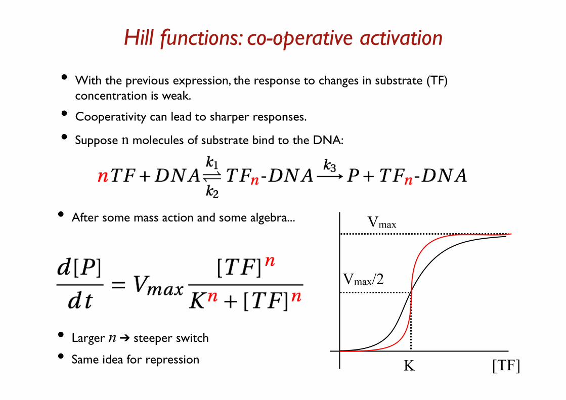
Hill functions: co-operative activation

• With the previous expression, the response to changes in substrate (TF) concentration is weak.

• Cooperativity can lead to sharper responses.

• Suppose n molecules of substrate bind to the DNA:

• After some mass action and some algebra...

[TF]

Vmax

Vmax/2

K

• Larger n ➔ steeper switch

• Same idea for repression

Hill functions: co-operative repression

• Suppose n molecules of substrate must bind to the DNA to block transcription:

• After some mass action and some algebra...

[TF]

Vmax

Vmax/2

K

• Larger n ➔ steeper ‘off ’ switch


• Auxin is a plant hormone, which stimulates degradation of Aux/IAAs. • Aux/IAAs repress their own transcription. • Hence Auxin stimulates Aux/IAA transcription.

ODE Example - Auxin signalling


Mass action:


Transcriptional regulation:

Equivalent to Shea-Ackers formulation (details for later)


Assumption Relaxation

The numbers of each molecular species are large enough to represent as continuous variables

Discrete models

Production and degradation processes are continuous

Discrete models

Outputs of processes begin to change as soon as the inputs change

Delay differential equations

Processes are deterministic Stochastic differential

equations

Spatial distribution in a cellular compartment is not important

Partial differential equations

ODE Models: Basic assumptions


Summary

The properties of a system can be represented by a set of variables that collectively constitute the state of a model

In dynamic models, the state is a dynamical variable (i.e. changes in time)

State evolution models encode mathematically the way that the state changes over time

ODEs are based on the assumption that the state changes continuously, at a rate that depends only on the current state

Summary


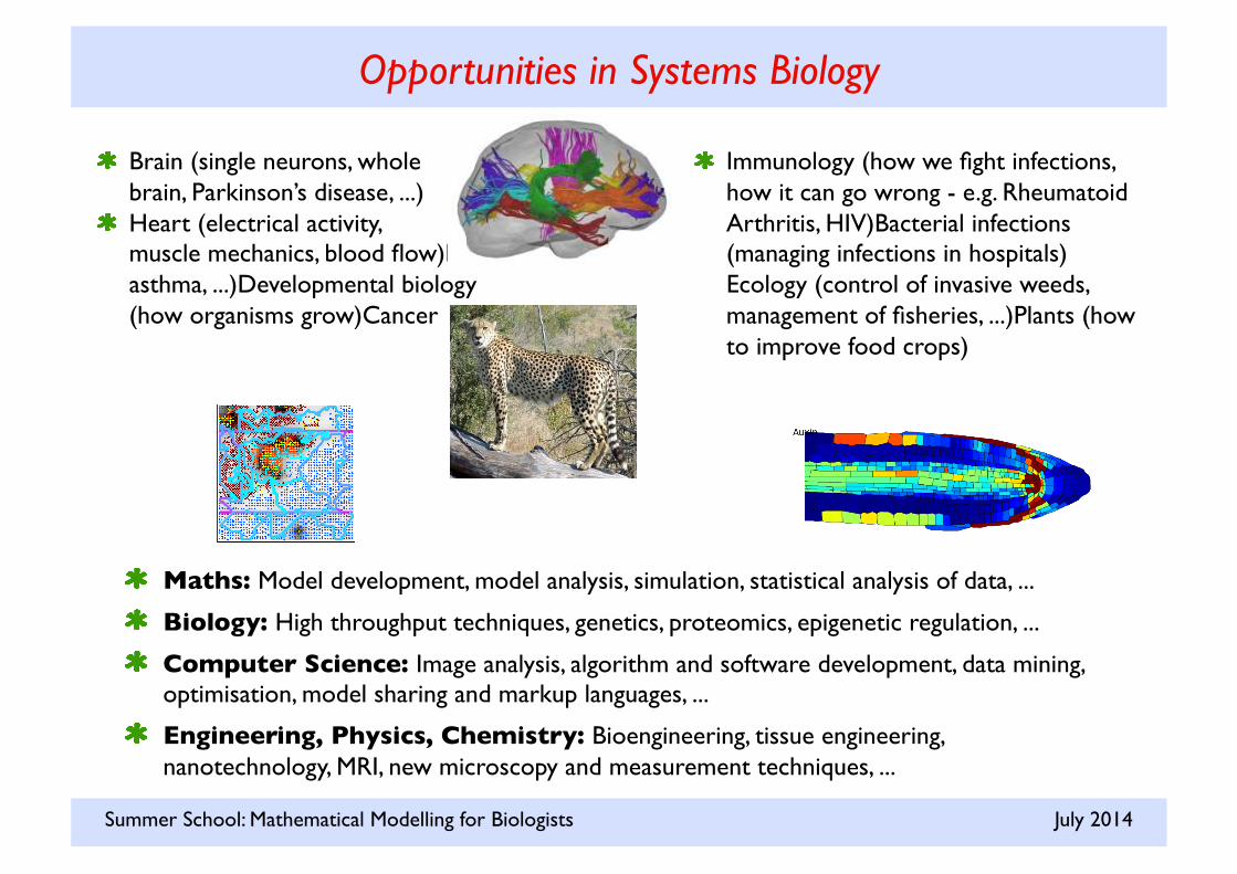
" Brain (single neurons, whole ��brain, Parkinson’s disease, ...)

" Heart (electrical activity, ��muscle mechanics, blood flow)Lungs (air flow, asthma, ...)Developmental biology ��(how organisms grow)Cancer

" Immunology (how we fight infections, how it can go wrong - e.g. Rheumatoid Arthritis, HIV)Bacterial infections (managing infections in hospitals) Ecology (control of invasive weeds, management of fisheries, ...)Plants (how to improve food crops)

Opportunities in Systems Biology

" Maths: Model development, model analysis, simulation, statistical analysis of data, ...

" Biology: High throughput techniques, genetics, proteomics, epigenetic regulation, ...

" Computer Science: Image analysis, algorithm and software development, data mining, optimisation, model sharing and markup languages, ...

" Engineering, Physics, Chemistry: Bioengineering, tissue engineering, nanotechnology, MRI, new microscopy and measurement techniques, ...

Documents

CPIB SUMMER SCHOOL 2014: INTRODUCTION TO BIOLOGICAL MODELLINGnick-monk.staff.shef.ac.uk/CPIB-Summer-School/lect1p1_slides_2014.pdf · Summer School: Mathematical Modelling for Biologists!