Embed Size (px)
Citation preview

CREW PROCEDURES ORBITAL GUIDANCE AND NAVIGATION PROGRAM
NAVIGATION SECTION
1.0 PROGRAM DESCRIPTIONThe CPB Guidance and Navigation Program, henceforth referred to
as AAP, is a modification set to Program BETELGEUSE. The program li-
brary currently exists on tapes I83 or l84 in the Building 35 Tape »
Library.AAP provides environment and estimated states for two vehicles,
rendezvous sensors and an inertial platform. These vehicles may be in
orbit about either the earth or moon.The navigation filter is a generalization of the Apollo-LM square-
root filter to two-vehicle estimation plus estimated sensor biases. Adetailed exposition of the theory of this filter may be found in refer-ences 1 and 2, and of the covariance advancement method in reference 3*
The filter accepts measurements of relative angle, range and/or range-rate, and updates the state of either or both vehicles in an optimalfashion.
The program is structured into a main overlay, and 1st and 2ndprimary overlays. The main overlay lists input/output devices, zerosworking core and sets values for sensor error models. The 1st primaryoverlay contains input/output routines, state and covariance integra-tors and the navigation package. The 2nd primary overlay contains sub-routines necessary to compute rendezvous maneuvers as currently defined.
By the setting of appropriate flags, AAP can be caused to run ineither single-run or monte-carlo modes. Data as specified by the useris collected at intervals on each cycle of a monte-carlo run, and storedon a local mass-storage file for later transference to a permanent datatape. This data may then be processed statistically by a separate pro-gram.
The following sections will deal with those portions of AAP whichconstitute the navigation function, and its controlling subroutines. Itwill be assumed that the user is otherwise familiar with standard BETEL-GEUSE functions and the operation of the guidance overlay,
2.0 PROGRAM CONTROLThe sequence of cards portrayed in figure 2.1 constitutes the con-
trolling set to read the program library, update corrections, load,execute and transfer run data from local to permanent storage. The fol-lowing notes corresponding to cards identified with the same number areprovided for clarity:
1. Creates local mass-storage file for monte-carlo data
2. Requests program libi'ary tape
3 . Copies program library to local file
4. Copies compile file to local file

5. Update changed subroutines from program library
6. Compile updated routines
7. Rewind update file
8. Copy changed subroutines into compile file
9. Request additional field length for loading
10. Load updated program
11. Set up overlay linkages
12. Reduce to execution field length
13. Execute
14. Create a dummy file
15. Rewind the program data storage file
16. Request the permanent data storage tape
17. Turn data storage tape past previously stored data
18. Copy new data onto tape
Should abnormal termination of the program occur, placement of an
EXIT, card following UNLOAD (DTARE) will cause control to be transferred
to the EXIT, card, and execution of all cards following. The card se-
quence from REWIND (fake) to UNLOAD (DTAEE) should be duplicated and placed
behind the EXIT, card, This^will prevent loss of data in the event of
abnormal termination. In order for a subroutine to be modified, it must
already exist in the tape program library. Attempts to add a previouslynon-existent subroutine will cause error termination. To amelioratethe effect of this restriction,, the first primary overlay contains five
dummy subroutines, OFENl to 0PEN5* These, may be modified as required to
provide currently undefined program operations.
3.0 REQUIRED INPUT DATAIn order to produce desired program operation, it is necessary to
specify sensor and lU error models, navigation initializing and control
information and platform alignment times. If maneuvers are to be per-formed, targeting data and instructions as to which will be stored for
later processing are also required. Vehicle state vectors and theircovariance are specified in the usual way for all BETELGEUSE programsrequiring such information.
2

3.1 HAED-WIRp CONSTANTSRendezvous sensors, alignments and maneuver applications are all
modelled by AAP as pure Gaussian processes. Values for the means andstandard deviations of these processes are set in program MAIN of the
main overlay by FORTRAN replacement statements. Figure 3*1 presents
the relevant portions of program MAIN with the subject variables under-
lined. A correction set of similar replacement statements must be con-
tained in the update portion of the operating deck if sensors beingmodelled have a different error model than that shown in figure 3.1j
VARS ACCELEROMETER SCALE FACTOR ERROR (DIMENSIONLESS)
VARA DELTA-V CUTOFF UNCERTAINTY (ET/SEC)
RVAR ACTUAL VALUE OF RANGE MEASUREMENT ERROR AS A FRACTION OFTOTAL RANGE (DIMENSIONLESS)
RVARMIN ACTUAL VALUE OF MINIMUM RANGE ERROR (FC)
WAR ACTUAL VALUE OF RANGE-RATE MEASUREMENT ERROR AS A FRACTIONOF TOTAL RANGE-RATE (DIMENSIONLESS)
WARMIN ACTUAL VALUE OF MINIMUM RANGE-RATE ERROR (ET/SEC)
VARAZ ACTUAL VALUE OF AZIMUTH MEASUREMENT ERROR (RADIANS)
VAREL ACTUAL VALUE OF ELEVATION MEASUREMENT ERROR (RADIANS)
Ms Ms ACTUAL VALUES 'OF RANGE, RANGE-RATE, AZIMUTH ANDELEVATION MEASUREMENT BIASES. THESE ARE SET INTHE FIRST VISIT TO THE SENSOR NOISE SUBROUTINEON THE BASIS OF THE VALUES OF B^, BVO, BAZOAND BELO
BRO ACTUAL VALUE OF RANGE BIAS ERROR (FD)
BVO ACTUAL VALUE OF RANGE-RATE BIAS ERROR (FC/SEC)
BAZO ACTUAL VALUE OF AZIMUTH BIAS ERROR (RADIANS)
BELO ACTUAL VALUE OF ELEVATION BIAS ERROR (RADIANS)
GDR ACTUAL VALUE OF GYRO DRIFT RATE ERROR (RADIANS/SEC)
ALIGNS ACTUAL VALUE OF INITIAL MIS-ALIGNMENT BIAS ERROR (RADIANS)
NFAMA INITIALIZER FOR MANEUVER APPLICATION ERRORS
NFAMB INITIALIZER FOR SENSOR BIAS ERRORS
O 3

ill
1 . t-lr.-oOLrCU T^:)Mol-c-teD ; ( F L
14.33.^1.F0LLTM CnMPLFTEn.stjouor
:4-.-3 4-.-9^*-.-F0F ypp
^ 14.34.1F.rOPYf^F( T^oFlw —1:4 ,-3 4-i-?^-. UMt fT/'. D-(-T
)’
4. ?F. (Kf^NjU “^FN^)
-7 frrHPf^-T ~i W )-
5 14.34.27.PFA0TNG T^P'JT
—l-4v3 9-.-i E-.'UP P A T E -C^'MPL'E T E—
14«33,t6.PTN'(T = r.C*^PTL^) .<r1
—i 4 •-7 F , -l a-i 1 7-i 7^^ C P-- SE COtJns-e o m p a t-ton —ti m e
14.3E..31 .PFWTND tL'^0) <1 —
14-36.37. PK updated—1 4'i-3 6-. .3 4"-INPUT U PD A TE D —
^
14-36.34. GNEVEC UPDATED—14.-3 6 r-3 4-5—DEL T A V UPfTATEO
14.36.34. STQPEl UPDATED
14.36.37. POPCUT UPDATEDI^t5“36-r3^.- " G P E TI3 “UPOA TED
36. ‘40. CPEN4 UPDATEDP ?65-4t'5-"OPENS —UPDA’TEO1'. 36.47. CLOD UPDATED
14.36.47. GIDSEL UPDATED1-4 --36-5 4-PtD0PYL“DC\'E14.36. 4P. PEL, 7000'^.
-n 4 ; 3 6 . 4 P . L O A 0 < X Y X '
—t^TS-TiT-T-E-rP Ft- ,• 6 0 ^-n
j,4.37.7F,AAP. <;1 45-3 n .-4 A ,-DOtt:rUT--COMPtP TEQ-
14-5?. 30. POLLTN COMPLETED.19T^7 .-6 2-.- EXT r —15.77.E7.PFWTND (FAKP)
<PL- --60000)
--lF^e7.E?.78E<J—
15.?ft.l7. (77 ASSIGNED). 1 7. PP WIND (D-’TAPP)-
16.73.17.AT)PYPF(nT^Dr,rAi<r,'’)—16-5-?PT-3^TrCPYf^F (S-’^A T',-rtT-A-P*^1-i
IE. ?P. 17. PEL c^Asr(^AKP)16.7P,17,'n;i. Crn
)
1 P , 7 p . 1. 4 . '•n 77 PL'^C^S WPTTT.E^'--t10^156^-.2p.E-n-.rp ' • 135 0.'3 70 SEC.• •2p.7n.pp 31''. 604 SEC.
T’igure 2.1 - AAP Control Cards

C LOAD ERROR MODELVARS-ltE-^VARA=lLE«i_
.C
RVAR^OtRVARMIN = 33 ^_
VVAR=4L3E-3VVARMIM=.43
VARAZ=g. E-3VAREL = 2.E-3
BR~0.BV=0«
BELrO*BRO£n_.
.BVO=0.BAZ0:^17.4SE-3
c«
GDR='1.45E-7
—
! ALIGMB=3.E-4NFAMA= 46728NFAMn= 12944NFAMC= 31171NFAMV= 22222
C _RV A RB= b'
,
RVARMMB = 33.VV_ARB=4. 3E-3VVARMNB=.43
VARAZB=2,E-3VARELB=2«E-3
C
Figure 3«1 Hard-wired constants

{
%
NFAMC INITIALIZER FOR PLATFORM MISALIGNMENT AND DRIFT ERRORS
NFAMV INITIALIZER FOR SENSOR RANDOM NOISE ERRORS
RVARB FILTER VALUE OF RANGE MEASUREMENT ERROR AS A FRACTION OFTOTAL RANGE (DIMENSIONLESS)
RVARMNB FILTER VALUE OF MINIMUM RANGE ERROR (FT)
WARB FILTER VALUE OF RANGE-RATE MEASUREMENT ERROR AS A FRACTIONOF TOTAL RANGE-RATE (DIMENSIONLESS)
WARMNB FILTER VALUE OF MINIMUM RANGE-RATE ERROR (FT/SEC)
VARAZB FILTER VALUE OF AZIMUTH MEASUREMENT ERROR (rMIANS)
VARELB FILTER VALUE OF ELEVATION MEASUREMENT ERROR (RADIANS)
All values are to be given l-sigina (standard deviation) includingsensor biases. Bias processes are considered as having a zero mean;these are constructed at the beginning of program execution and be-come the mean value of any subsequent random process . To the extent thatit models or ignores sensor biases, and compensates for random noisein the wei^ting process
,the filter contains a model of every known
random process affecting the value of a measurement. The difference be-tween the actual value of a random process, and the filter value, isthat in general the actual values can only be guessed at. Hence theactual and filter values are not in general the same, and it is cus-tomary to set the filter value larger than the largest expected valueof the actual errors.
3.2 INPUT DATA CARDSIn addition to normal BETELGEUSE input cards, additional cards
are defined which control the storage of data at selected maneuvers,the performance of navigation processes and the time of platformalignments. Also, some of the BETELGEUSE input features areutilized in the normal way to set flags and support the input ofother required data. These will now be examined on a card-by-card basisas to placement and content:
CARD #1, INTEGER PARAMETER, l4l5IDENT, Cl-C5> Program will execute number of monte-carlo cycles
equal to IDENT
NP, C6-ei0, Number of P-array variables in data file
NINT, CII-CI5 , Starting value of NGUIDE (determine's whichmaneuver of rendezvous sequence is first)
NFIRST, C16-C20, BETELGEUSE initial condition option
4
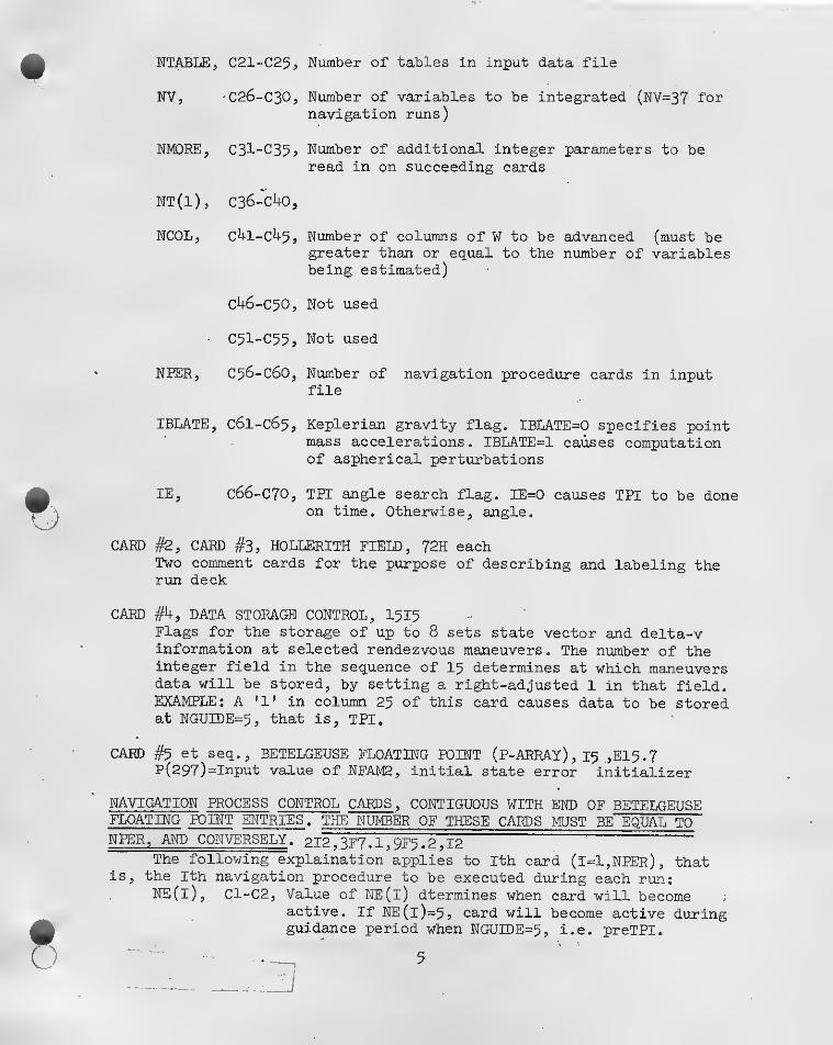
NTABLE, C21-C25
NV, C26-C30
NMORE, C31-C35
NT(1), C36-c4o
NCOL, c4i-c45
c46-C50
C51-C55
NPER, C56-C6O
IBLATE, C6I-C65
IE, C66-C70;
Number of tables in input data file
Number of variables to be integrated (NV=37 fornavigation runs)
Number of additional integer parameters to beread in on succeeding cards
Number of columns of W to be advanced (must begreater than or equal to the number of variablesbeing estimated)
Not used
Not used
Number of navigation procedure cards in inputfile
Keplerian gravity flag. IBLATE=0 specifies pointmass accelerations. IBIiATE=l causes computationof aspherical perturbations
TPI angle search flag. IE=0 causes TPI to be doneon time. Otherwise, angle.
CARD #2, CARD #3, HOLr.ERITH FIELD, 72H eachTwo comment cards for the purpose of describing and labeling therun deck
CARD #4, DATA STORAGE CONTROL, I 5I5Flags for the storage of up to 8 sets state vector and delta-vinformation at selected rendezvous maneuvers. The number of theinteger field in the sequence of I5 determines at which maneuversdata will be stored, by setting a right-adjusted 1 in that field.EXAMPLE: A '1' in column 25 of this card causes data to be storedat NGUIDE=5, that is, TPI.
CARD #5 et seq., BETELGEUSE FLOATING POINT (P-ARRAY),I5 ?E15.7P(297)=Input value of NFAM2, initial state error initializer
NAVIGATION PROCESS CONTROL CARDS, CONTIGUOUS WITH END OF BETELGEUSEFLOATING POINT ENTRIES . THE NUMBER OF THESE CARDS MUST BE EQUAL TONFER, AND CONVERSELY . 212 , 3F7. 1 , 9F5 .2 .12
The following explaination applies to Ith card (r=l,NPER), thatis, the Ith navigation procedure to be executed during each run:
NE(I), C1-C2, Value of NE(l) dtermines when card will becomeactive. If NE(l)=5> card will become active duringguidance period when NGUrDE=5, i.e. preTPI.
I
j
5
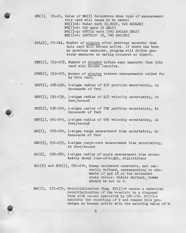
NM(i), C3-C4, Value of NM(l) determines what type of measurementthis card will cause to be taken:NM(l)=l: Radar mark (E,RD0T, TWO ANGLES)NM(I)=2: VHF mark (R ONLY)NM(l)=3:, OPTICS mark (TWO ANGLES ONLY)NM(i)=4: shuttle? (R, TWO ANGLES)
DTL(I), C5-011, Number of minutes after previous maneuver thatthis card will become active. If there has beenno previous maneuver, program will define pre-vious maneuver as having occurred at time=0.
DTN(I), C12-C18, Number of minutes before next maneuver that thiscard will become inactive,
DTM(I), C19-C25, Number of minutes between measurements called forby this card.
USP(l), C26-C30, 1-sigma radius of S/C position uncertainty, inthousands of feet
USV(l), C31-C35 j l“Sigma radius of S/C velocity uncertainty, in
XJTP(l), C36-C40, 1-sigma radius of TGT position uncertainty, inthousands of feet
UTV(l), c41-c45, 1-sigma radius of TGT velocity uncertainty, infeet/second
SR(i), c46-C50, 1-sigma range measurement bias uncertainty, in'thousands of feet
SJffi(l), C5l"C55j 1-sigma range-rate measurement bias uncertainty,in feet/second
SO(l), C56-C6O, 1-sigma radius of angle measurement bias uncer-tainty about line-of-sight, milliradians
SCl(l) and SC2(l), C6l-C70, Dummy estimated constants, not cur-rently defined, corresponding to ele-ments 17 and 18 of the estimatedstate vector. Unless defined, theseshould be set to 0.
NW(l), C71-C72, Reinitialization flag. NW(l)=0 causes a sphericalreinitialization of the W-matrix to a diagonalform with values specified by C26-C70* NT\r(l)=l
inhibits the resetting of W and causes this pro-cedure to become active with the existing value of W.
6
215.9674, 36, '54 -75,881-2-i.-^i-3-5-6-8-i 36» I 3 8
—
,98 25557.59 173,. 48 B 127 .
-i^2 2555-6r.-5-a— 1
-8^ 193.-2-8-5-r
-2.84---TtTT
-4.49-^4t1-3-
-: TAX'nrtrrT-'-s j w 1 1 xoiiu.u
XS(B9F) YS(89F) Z3(BRF) XSD(BRF) YSD(BRF) ZSBCBRF) XT(8RF) YT(3RF) ZT <BRF) XTD(BRF) ZTD(BR F)
42'>21 3 6. -4 :. 8818 6 . 12 5 05, 6 0 22276. 3^ ?^>3"7u 42420^^ -3088352, -2J85997&. 1Z507.54 ''
424.-&9a. -3^96558. -30862699. 125J4.2C 22275.49 -785.5 3 4240567. -3G96932. -2G862371. 12505,78 22279.45 -763. .9
-X52-<MF)—1541.
-Y-SB-FMF-)-
-35 96.
CARTESIftM ST^TE ERRORS .IN MEASUREMENT FRAMEZ S F<MF9——X-S0E-<MF-)—YSQE < MF-) ^X-ft-tMF-)—
2677, -8,93 -7.27 -3,57 1047,
relative state errors=- = r^ = =^--^ B-I A -S-E-S-TI MA H-GN—==R-RATE azimuth FLEV SCI 302 XRE(MF)
"Temf-)—-8704.
YRE(MF)
S-OOT
2682. -8.84•TtlEIMm—^rTOe(MF)
-7.62 -3.80
ZRF(MF) XRDE<MF) YRDE(MF) ZROE(MF)_ « i-L rr rr O 9
SD-COEL DELTA-H DELH-OOT
-Zx.-'L-
R-RATE AZIMUTH REL ELEV MF-L3 0 UR6,944 35.793- RAO-i7--URO
-4.95 4.483 32.152 VHP 0 UAZ4 1.-395-- OPT—R—UE-t
17.5
ST-4NG4
3/C 5349. 3733.fGT 5-349, 873-7-,
—
BIAS 0 . . n D 0
43.5 FNG
A4pJ-0f+S E9.36 11.71
— 9 * «*6—11 ,-71;
—-4 • 6 2
15839 ETAOI
- 1 .7 -:
-.689 DVNOR/ ^ ^ rvi # I ^
1,701 DVOOP
ee^ R-IA NO £ OF RE tA-TI-Vc—0RRCHRS—1 HFl
144E+11 .452E+0i .566E-31 .228E-01 .591E-02 .386E-03Ti3L955-4-Hi:6-9E+t-2 tH rt-SSe-ei ^4--3-3 E+O-H—i-e4 6E -0
1
,02721 , 15186 1 ,145E + 31 .454E-03 .629E-02 .225E-01
92164 .15666 .10274I.278E-P1 •574E-a4-T09129l-i-226E-01
->4 A V IG A T-i-GN-B URN -E 5 T I MA T E I S -0 U=
ACTUAL COMPONENTS WrR5 DU=^€-541-2 OV“2.434 OV=
—41^-44
—
4.294 DW: .187
2 i5 . 9^5 r
•
^‘4GI-fL^OE -t-AT^^UOi
19,5.9 -75.795
BETEL GEUSE STATE 1380.CrT^A-T-E HOR-VEE HEA-CWS X-B^R—-3.19 25561.33 -17:, 7. 9 “31, -56. -.11 -.23
CARTESIAN -STAT l33j-i-8

ALIGNMENT CONTROL CARD , CONTIGUOUS WITH THE END OF NAVIGATION PROCESSCONTROL CARDS . THIS CARD MUST BE PRESENT, EVEN IF BLANK . i2,10E7.1
Program will read up to 10 decimal fields on card, following in-
teger field. Integer in first two columns determines how many F-fieldswill be read in subsequent columns. Subsequent columns contain the times,in seconds, of desired platform realignments during each run. If cardis blank, an alignment is automatically performed at time=0,
INPUT STATE COVARIANCE MATRIX, IMvIED lATELY FOLLOWING ALIGNMENT CARD.THIS MATRIX MUST BE PRESENT WITH DIMENSION 24 x 24 IfTT297) IS OTHER
THAN ZERO.^
INPUT TABLES CALLED FOR m NTABLE , IMMEDIATELY FOLLOWING INPUT COVARI-
ANCE MATRIX.THESE TABLES MUST BE PRESENT IF NTABLE IS GREATER THAN ZERO.
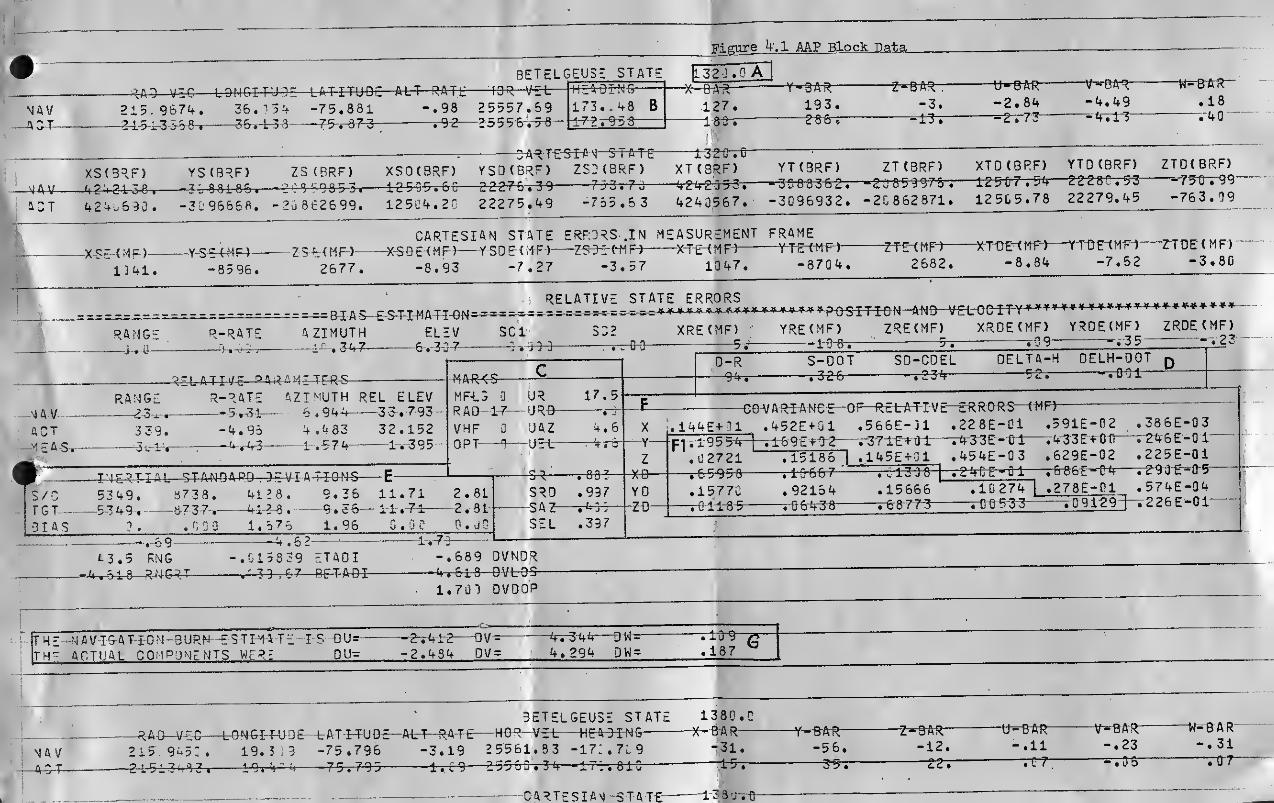
4.0 OUTPUTProgram AAP originates printed and mass storage output. Printed
output is originated by the 2nd primary overlay during maneuver compu-tations, by the 1st primary overlay during maneuver applications, andat each platform alignment. Block data on all vehicle states, and thestatus of the navigation, is printed periodically as specified by theuser, A sample of such output is shown in figure 4.1 and will be dis-cussed below. Block data print interval is controlled by setting P(9)equal to the desired print interval, in seconds. Block data is auto-matically printed every time the guidance (2nd) overlay is called, orwhenever the W-matrix is reinitialized.
Area A; Time, in seconds, of the block print.
' o' oArea B: Azimuth of ground track; east is 0 , south is 90 j etc,
Cartesian State: Earth centered inertial frame (BRF)
Cartesian State Errors in Measurement Frame (MF): Measurement frame is
defined as follows
-
UNIT(2^)=UNIT(Y^ X.
UNIT(Y^)=UNIT(^^.^:-.Rg/^)
UNIT(^)=UNIT(^/^ X Y^)
XSE, YSE, ZSE: SPACECRAFT POSITION ERROR'
XSDE, YSDE, ZSDE: SPACECRAFT VELOCITY ERROR- STATE ERRORS
XTE, YTE, ZTE: TARGET POSITION ERROR IN MFXTDE, YTDE, ZTDE: TARGET VELOCITY ERROR
7

IRelative State Errors: Bias estimation portion is the estimated bias
minus actual bias for each sensor in ft, ftps-j mr.
XEE,. YRE, ZRE: RELATIVE POSITION ERRORS IN ME (ft)
XRDE, yPDE, ZRDE: RELATIVE VELOCITY ERRORS IN ME (fps)
Relative Parameters: Navigated and actual values of range, range-rate,
azimuth and elevation in the local vertical in-
plane frame. Measured values of these quantities
have noise and biases added and are given in the
estimated measurement frame. Units are ft, fps, deg.
Area C: Navigation Status
MFLG: Filter status flag: MFLG=0 Marking is enabled on any pro-
cedure active during this period.
MFLG=1 Marking is suspended because of
final maneuver computation or
recycleMFLG=2 Final comp has been done and the
filter is waiting for ignition
before resuming updates
RAD: Number of radar marks since last W-reinitialization
VHF: Number of VHF marks since last W-reinitialization
OPT: Number of angle marks since last W-reinitialization
UR; State uncertainty in next range measurement (ft)
URD: State uncertainty^ in next r-rate measurement (fps)
UAZ: State uncertainty in next azimuth measurement (mr)
UEL: State uncertainty in next elevation measurement (mr)>
SR: Wei^ting given a-priori estimate of range on last mark (A
value of 1.0 indicates 100^ confidence )
SRD; Same as above for r-rate
SAZ: Same as above for azimuth
SEL: Same as above for elevation
Area D: Coelliptical relative errors at phase match. Space craft is
advanced to phase match with target and curvilinear errors are
computed
O8
S-R: Down-range error
S-DOT: Horizontal speed error
^-COEL: Horizontal speed error minus speed error if vehicle errors
were coelliptical
DELTA-H: Vertical position error
DELH-DOT: Vertical speed error
Area E: List of square roots of the diagonal terms of the filter co-
variance matrix. 1-sigma estimated uncertainty in the value
of each estimated quantity, expressed in measurement frame.
Vehicle rows are in the order of X, Y, 2, XD, YD, 2D; bias
row is in order of R, ROOT, AZ, EL, SC1,SC2.
* Area F: Covariance of relative errors in the measurement frame. Dia-gonal elements are 1-sigma uncertainties in each of the framedirections in the order of X, Y, Z, XD, YD, ZD. Lower leftportion (Area Fl) is array of correlation coefficients.
Area G: Estimated and actual maneuver. The navigation burn estimateis that computed from the estimated vehicle states ^ The actualvalue is that maneuver actually applied in view of platformdrift, scale factor error and cutoff uncertainty.
MASS DATA STORAGEOn- each cycle of a monte-carlo set, AAP stores up to 350 items of
data on a locally created file, in unformatted form, for later trans-
ference to a permanent data storage tape. Before writing the local file,
the program writes the date., time and number of cycles (one word each)
on the beginning of the file. At the end of each cycle, the DATA arrayof 350 words is dumped on the file. These words are allotted as follows;
DATA(1)=L00P, Current value of the monte-carlo cycle index>
DATA(2)-DATA(249) 5Up to 8 sets of state vector and maneuver in-
formation stored for selected maneuvers (see
CARD #4). Each set consists of 3I elements:1-6: S/C actual BRF vector7-12: TGT actual BRF vector13-18: S/C navigated BRF vector19-24: TGT navigated BRF vector25-27 J Maneuver computed from actual states28-30 : Maneuver computed from estimated states31 : Time of ignition
9
I
j

DATA(251)“DATA(320) , Up to ten sets of platform alignment informa-tion. Each set consists of 7 elements:1-3: Platform angular drift rates (X^Y^Z)4-6 : Initial platform misalignment {X,i,Z)7: Time of alignment
DATA(321)-DATA(350) , Arbitrary output specified by user.
Regardless of which maneuver is the first with a data storage flagset, the state vector/maneuver data is stacked, 3I elements at a time,beginning in DATA(2). All quantities are output in fundamental unitsof feet, seconds and radians. A dump of the DATA array in the indicatedformat is performed at the termination of each cycle.
5 . 0 PROGRAM MECHANIZATIONThis section will discuss the implementation of the navigation
function down to the level of FORTRAN code. As a preliminary, the assignment and definition of all variables associated with the navigation willbe reviewed.
MASTER COMMON AND EQUIVALENCE LIST
BLANK COMMON: VAR(5600)
LABEL COMMON: DELV
GARB
ALIG
BV
BETELGEUSE BLANK COMMON
LISTS VARS, VARA, NFAMA, SDr3) FORUSE IN MANEUVER APPLICATION ROUTINE,VARS , VARA , AND NFAMA ARE DISCUSSEDIN SECTION 3.1- SD(3) ARE THREEACCELEROMETER SCALE FACTORS CREATEDON FIRST VISIT TO DELTAV (MANEUVERAPPLICATION),
LISTS ACTUAL STATISTICS OF SENSORERRORS FOR USE BY SENSOR NOISE ROU-TINE ( GARBAGE ) . SEE SECTION 3.1.
LISTS ACTUAL STATISTICS OF PLATFORMALIGNMENT AND DRIFT ERRORS FOR USEBY PLAT ALIGN ROUTINE (ALIGN). SEESECTION 3.1.
LISTS FILTER STATISTICS OF SENSORERRORS FOR USE BY GEOMETRY VECTORSUBROUTINE ( BVEC ). SEE SECTION 3.1.
10
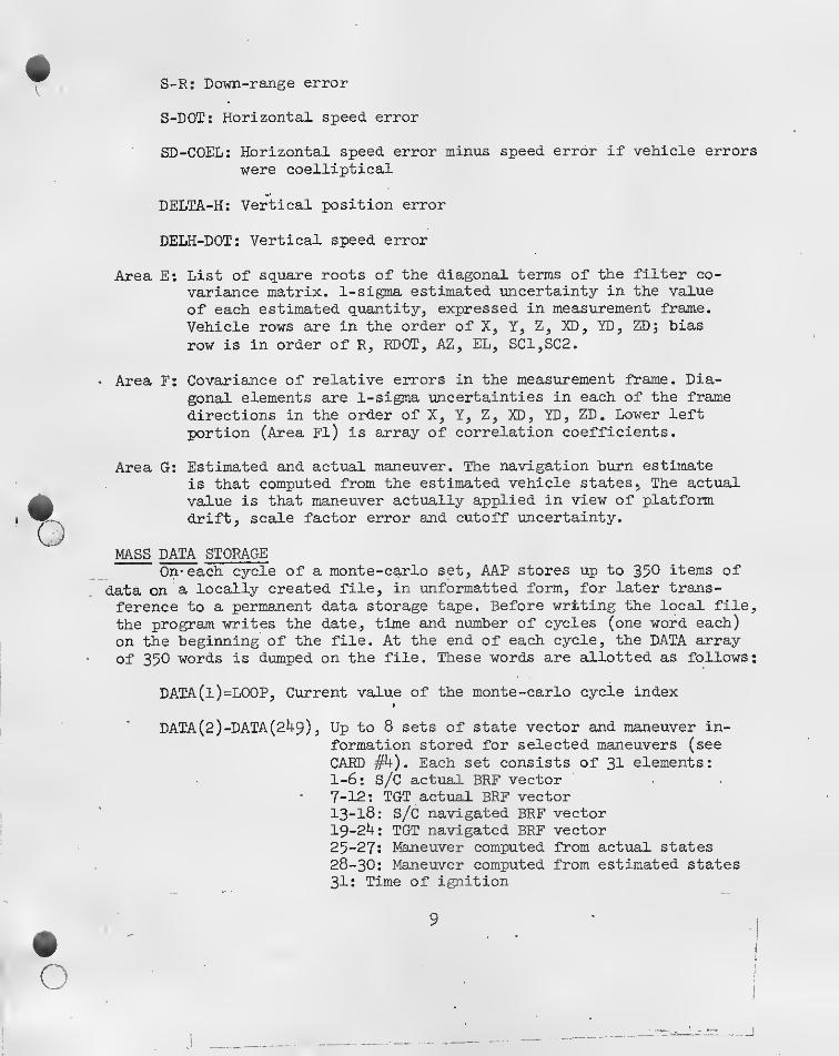
DIMENSIONED AREIAYS USED BY NAVIGATION
INTEGRATED VARIABLES
DERIVATIVES WRT TIME
INTEGER PARAMETERS
BETELGEUSE WORKING ARRAY
NAVIGATION STORAGE ARRAY
NAVIGATION SCRATCH PAD
MONTE-CARLO MASS DATA STORAGE
INPUT STATE VECTOR COVARIANCE MATRIX
MEASURED RELATIVE PARAMETERS
CURRENT VALUE OF MEASURED RELATIVE \(V*-
RANDOM NOISE
ARRAY OF CONTROL TIMES FOR GNEXEC
ESTIMATED TRANSFORMATION MATRIX
FROM BRF TO PLATFORM AXES
XNBNCs), YNEN(3),
ZNBN(3) estimated navigation BASE UNIT
VECTORS
ne(io) see section 3.2
NM(IO)
DTL(IO)
DTN(IO)
DTM(IO)
USP(IO)
USV(IO)
UTP(IO)
UTV(IO) ” " " '
Y(IOO)
DYDX(IOO)
NTEGER(IOO)
P(5000)
SAVE
(
950 )
BLK(700)
DATA
(
350 )
C0V(24,24)
QQ(4)
SIG(4)
C(10)
REFMAT(3,3)
o11
)WING, - COMMON
IS BLAN]^VAR
UlO /AR(56C-D » -Y(iOa> j- DY3X (IlO) , > j
- FIRST Y< 10 u)
' 0(1-00), M5jOO)NTEGER (1 J - ) , u ixu J / ,
/ALFNCE- V VAR ( 1) , Y ( 1 ) )
(VARdCi) ,OYOX(l) )
^.VAR.X2-^l-)-,a-(l-)4-r-T-%OT(VAR(3Q1) ,FIRSTY(1 )
)
...(VAR(4C1) ,NTcGER(l) )
(VAR(5ji ) ,0 (1) )
.XVAR(6wi) Cl) )
>JSION SA VE(950) , BLK(7O0
/ALENCE-—(S-<-3-5-0 )-r-SA VE-( 1 )-)-
CP(13[lu) ,3LK(i))
,P (1)
3LK(7O0) , 3 ATA (35C ) , C0V(24,24)AA/p-.n
(PCl^yij / ,-.>i_rsvx//
(P(4074) ,OATA (1) )-
(PC4424) ,CnV(i,l)
)
'JSION 00 C4) ,-SIG (4)-, C (10) ,- REFMAT <3,- 3) ,
ZN3N(3), NEClij), NM(li), DTL(IC), OTN(lc), w.-..-
USP-(-iO->-,—USV (-l-0')-,-N TP <-i"c-) T- UT V ( 10 )-r—SR(-l-0 )'r‘-SRO (-
trrx f A \ cr-ifin^. SC 2(10), NW(IC), TLMClL), NS(3)- ZN8E(3>-
XNfjN (3) ,
,
YN3N(3)DTM (iJ)
SRO (-10-)
TLMXNBE (3) ,• YNDE(3) ,
h'Uf^UU 1
—POPOUT”POPOUT
-- POPOUTPOPOUT
-POPOUTPCPOUT—POPOUT-POPOUT
-PCPOUTPOPOUT
-POPOUTPOPOUT
—PGPOUT-PCPOUT
— POPOUTPOPOUT
— PCPOUTPOPOUT—POPOUT
SO (10) , SCI (10) , 'S'JdilJ)
'ZT-Z-(4) ,—SZ (4) ,--T ALT GN ( 1 u
X<18), WE(1B,27)XLVE(3) ,YLV£{3) ,ZLVE(3)-,XLVN(3) ,YLVN(3) ,ZLVN(3)
ENCE (SAVE (1) ,00 £1) ) , f^ I ! ! I ,
.
VALENCE (SAVE .
-(SA-V E-(-9->-, G
. (SAVE(28) ,XN9N(1) ),' (SAVE (34 ) , ZN3N (1) )
/ . (SAVE £47) ,NH £1) )
,
Ixl-.CSAVE(67) ,0TN(1)) ,-
(SAVE (87 ) ,US° (1) )
,
(5AVc-( l-^:-7-) ,-UTP < 1-)-)-,-
CSAVEC127) ,SR£1))
,
(SAVE (147) , SO(l) ) ,
£SAVE£5) ;
(S A VE C 19 ) , RE F M AT-( l','i-H-
(SAVE (31) ,YNBN (1 ) )
(SAVE (37 ), ME (1) )-
:SAVEC57) ,OTL(l)
)
(SAVE(77),DTM(1) )-"
(SAVE{97) ,USV(1) )
<-SAVE.(117),UTV(l) )-
(SAVE £137) ,SRO (1)
)
r A tir- r A c T \ C‘ n A f A
I b A V t \ 1 i M ^ V X / /
(SAVE(147),S0(1)) , (SAVE (157) ,SC1 (1 )
)
(SAVE (167) ,SC2 (1) ) , (S A VE ( 1 7 7 ) , N W ( 1) )
•(SAVE (187) , TLM (1) ) ,(SAVE (i97),NS(l)>
/cA\/rf7::f».7T7(l)). (SAVE(234),SZ(i))(SAVE(218> jNALTGN)
\/ AfCt C f A \
POPOUT-PCPOUTPOPOUT
—NCSHITPOPOUT
—POPOUT-POPOUT
—POPOUTPOPOUT
— POPOUTPOPOUT
—POPOUT--POPOUT
-POPOUTPOPOUT
--POPOUT
0
7
3—9-
1311121314-45-
1617131923212223242526
- 27-
232933
1
31-3233
-3435
• 36-
37-33-
3943
4142
(S^VE iZi' L ) f i. i L \ Lt / f
-(-SAVE-(2-.’-8 )-rI al ign (1 ) (SAVE ( 21 8) , MAL IGN >—
(SAVE(229),XN3E(1)) ,(SAVE(232),YNBE(1))
. - - ;sAVE(253) ,X £1) )-
l-bA V L'V C-.-'-O HUlsJ'N Vi '
(SAVE(229),XN3E(1))
,
(SAVEC235) ,ZN9E£1)) -
(SAVE (276) , WE (1, 1)
)
(NTEGER(53) ,ICOMP)
YALCNCE (SAVE (762 ) , XLVE (1 )
)
tSAVEtrbi^)»XLVt^l(SAVE-(7o5-)-,-YL-V£ £-1) )
(SAVE (768) , ZL VI (1)
)
(SAVE (771)
, XL VN (1 )
)
(SAVZ(774) ,YLVN(1))(777 ) , ZL VN £1) )
POPOUT 43
POPOUT" 44POPOUT 45P OPOUT 4bPOPOUT 47POPOUT --- 45-
NOSHIT 2
NOSH i-J
NOSHIT—5"
4
NOSHITNCSHIT
"5
6
NOSH IT"
- j
POPOUT 49
FIGURE 5. .1 ST™ARD_ COMMON BLOCK
coc 66CC FTN V3.0-P3C8 OPT=l 06/29/72 ^9.17,0^

f SR(IO) SEE SECTION 3-2
TSED(IO) It tt II
so(io) It II ti
SC1(10),SC2(10) It II 11
NW(lO) ti tt ti
.TLM(IO) STORED TIME OF THE LAST MARK ON
EACH NAVIGATION PROCEDURE
NS(3) NUMBER OF MARKS SINCE W-RELNITIAL-IZATION ON RADAR, VHF AND OPTICS
ztz(4) A PRIORI UNCERTAINTY IN VALUE OFSENSOR MEASUREMENT
SZ(4) WEIGHTING ON A PRIORI ESTIMATE OFSENSOR MEASUREMENT
TALIGN(IO) STORED TIMES OF PLATFORM ALIGNMENTSSEE SECTION 3.2
fXNBE(3) 5^2(3),Z])IBE(3)
ACTUAL NAVIGATION BASE UNIT VECTORS
X(18) LOCAL STORAGE FOR ESTIMATED CAR-TESIAN STATE
W^!(i8 , 18 ) THE FAMOUS W-MATRIX
XLVE(3),YLVE(3') ACTUAL LOCAL VERTICAL UNIT VECTORSZLVE(3)
XLW(3),YLVW(3)ZLVN(3)
ESTIMATED LOCAL VERTICAL UNITVECTORS
DRIFT (3) INTEGRATED PLATFORM MISALIGNMENTANGLES
RATE(3) PLATFORM GYRO .DRIPT RATES
Subroutines which utilize the BLK array for intermediate localcomputations define and equivalence local variables as required. Thesewill be individual^ discussed in the section on subroutine structure.Figure 5 .I presents the standard navigation common block . In additionto the equivalences shown, the following are scattered throughout:
•o
12

NTEGER(29), NGUIDE CURRENT VALUE OF NGUIDE
30 ICOMP NAVIGATION STATUS FLAG (SEE MFLG,
SECTION 4.0, AREA C)
31 ISTEP CmXEC INTEGRATION STEP-SIZE MANAGE
MENT FTiAG
32 NOVER .OVERLAY RETURN MANAGEMENT MG
33 LIGK CURRENT NUMBER OF PLATFORM ALIGN-MENTS ALREADY PERFORMED
34 NOT DEFINED
35 RGATE BRAKING GATE COUNTER
36 NBREL SET WHEN IN BRAKING PHASE
42 RLIRE PRINTED OUTPUT LINE COUNTER
C(1 )TW TIME TAG ON W-MATRIX
8 STEP SAVED VALUE OF INPUT INTEGRATION
STEP SIZE
9 T2 SYNCH STEP SIZE FOR FINAL PASS AF-
TER MANEUVER APPLICATION
10 TGN TIME FROM NEXT IGNITION
-
13

u
5.1 FUNCTIONAL DESCRIPTIONIn spite of the overlay structure, the actual operation of AAP
is practically indestinguishable from that of the traditional BETEL-
GEUSE program. The guidance overlay (2nd) acts like a subroutine whichwhen called, computes a maneuver specified by the current value of
NGUIDE. Other than the filter computation routines, the most significantaddition to the program is the guidance and navigation executive, whichcontrols the taking of navigation marks and the calling of the guidanceoverlay. The following is a list of subroutines peculiar to or modifiedby the presence of the navigation function:
.
MAIN REFERENCES MONTE-CARLO MASS STORAGE FILE (TAPE77=STAT)SETS VALUES FOR ERROR MODELS BY REPLACEMENT
INPUT-). ). ‘••.'i!.
Ca^EXEC
DELTA
V
STOREl
OUTDAT
POFQUT
CART1 , CART2
SETY
REL
HAS OVERLAY RETURN FLAG (NOVER), CALL TO GNEXEC , CALL TOSETY , CALL TO POPOUT , ENTRY POINT FOR COVARIANCE ADVANCE-MENT (ENTRY RKW), INTEGRATES PLATFORM DRIFTS
WRITES ON MASS DATA STORAGE TAPE (77), READS DATA STORAGECONTROL FLAGS, READS NAVIGATION PROCESS CONTROL CARDS,READS ALIGNMENT CONTROL CARD, INITIALIZES GUIDANCE, NAVI-GATION AND ALIGNMENT PARAMETERS, CALLS ALIGN AND SETY
CONTROLS TAKING OF NAVIGATION MARKS, COMPUTATION ANDAPPLICATION OF MANEUVERS
APPLIES AN ESTIMATED AND ACTUAL MANEUVER TO THE ESTIMATEDAND ACTUAL STATES
STORES 31 ELEMENTS OF STATE VECTOR AND MANEUVER INFOR-MATION AT SELECTED MANEUVERS
DUMPS THE MASS STORAGE MONTE-CARLO DATA AT THE END OFEACH CYCLE
COMPUTES ACTUAL, ESTIMATED AND MEASURED RELATIVE PARA-METERS, SETS UP VECTORS AND FILTER STATUS DATA, PRINTSBLOCK DATA AS REQUIRED
SUBROUTINE CONVERTS BETELGEUSE VECTOR TO CARTESIAN (CARTl),OR A CARTESIAN VECTOR TO BETELGEUSE (CART2 )
LOADS CARTESIAN FORM OF ESTIMATED BETELGEUSE STATE INTOY ARRAY. CURRENTLY ONLY ONE INSTRUCTION IS ACTIVE- ALLCALLS TO SETY MAY BE REPLACED WITH THE STATEMENT CALLCARTl(Y(3BTrY(2))
COMPUTES RELATIVE PARAMETERS (R, RDOT, AZ, EL) GIVENCARTESIAN VECTOR AND UNIT VECTORS OF MEASUREMENT FRAME
14

SETUP
GARBAGE
ALIGN
SETS UP AN OUTPUT FORM OF THE BETELGEUSE VECTOR
CREATES INITIAL SENSOR BIASES AND ADDS RANDOM NOISE TO
RELATIVE PARAMETERS
CREATES INITIAL PLATFORM DRIET RATES, DEFINES A REFMAT
AND SETS MISALIGNMENT BIASES FOR EACH ALIGNMENT
P20 LOCAL SUPERVISORY ROUTINE FOR TAKING A NAVIGATION MARK
ADVW
BVEC
FILTER
COVARIANCE INTEGRATING SUBROUTINE
CALCULATES AND CONSTRUCTS REQUIRED GEOMETRY VECTORS FOR
FILTER
CALCULATES WEIGHTING VECTOR, UIDATES STATE AND COVARIANCE
OFENl-OPEN^ DUMMY SUBROUTINES FOR USER DEFINED FUNCTIONS
The navigation function operates on a cartesian vector which is
created periodically from the estmated BETELGEUSE state vector. This
cartesian vector, althou^ not itself integrated, is stored in the
Y array. Because it is req.uired for covariance advancement, the pre-
vious value of this vector ,called X, is stored in the SAVE array
from the previous visit to ADVW . The allocation of the Y array to
state and other variables is as follows
;
Y(l),
Y(2)-Y(13)
y(i4)-y(19)
Y(20)-Y(3I)
y(32)-Y(37)
y(38)-Y(49)
Y(50)-Y(55)
y( 98 )-y(ioo)
TIME
ESTIMATED BETELGEUSE STATE
ESTIMATED VALUES OF SENSOR BIASES
ACTUAL BETELGEUSE STATE
ACTUAL VALUE OF, SENSOR BIASES
ESTIMATED CARTESIAN STATE
ESTIMATED VALUE OF SENSOR BIASES (SAME AS Y(14)-Y(19))
TOTAL INTEGRATED PLATFORM DRIET ANGLES . THESE ARE
EQUIVALENCED TO DRIFT
(
3 ) IN SUBROUTINE ALIGN . ALSO,
THEIR DERIVATIVES, BATEJs), ARE EQUIVALENCED TO DYDX(98)-
DYDX(IOO) IN ALIGN .
o15
5.2 COMPUTATIONAL ORGANIZATIONFigure 5.2.1 presents the interfaces of the major navigation func-
tional subroutines. The remaining part of this section will present the
K)RTRAN code used to implement this function, with flow diagrams and
explainatory notes where appi^riate. The following comments refer to
Figure 5 •2.1:
MAIN Main program of main overlay.
DUMMYl Called by MAIN to bring in first primary overlay AAP(1,0)
RK Integrating subroutine for (l,0). Also called at ENTRYRKW by ADVW for integration of W-matrix.
INPUT Controls input of data to program. Called by RK at the
beginning of each monte-carlo cycle
ALIGN Simulates performance of platform alignment. Called byINPUT at beginning of program execution, and by GNEXECat times defined by alignment control card.
POPOUT Handles computation of actual, estimated and measuredrelative quantities for output and navigation. Computesand organizes for output other quantities of interest.
Prints block data at intervals defined by P(9)s andwhenever called throu^ ENTRY POPW by GNEXEC. Computationsection of POPOUT will be executed when POPOUT is calledon each pass through RK, even if print is inhibited.
OVERLAY 2 Called in from GNEXEC at termination of the last markingprocedure in a premaneuver period. Because return fromAAP(2,0) is-to DUMMYl and RK, special provision is madein the program to return to the next instruction in GNEXECfollowing the call to AAP(2,0), This is accomplished bythe setting of the NOVER flag.
I
GNEXEC Executive routine. Controls taking of navigation marks,performance of platform alignments and computation ofmaneuvers. Called once each pass through RK.
DELTAV Applies maneuvers computed by guidance overlay to actualand estimated states. Called from GNEXEC. Also callsADVW to advance covariance to time of ignition.
STOREl Loads state vector and delta-v data into DATA array fordump to mass storage at end of cycle. Called from GNEXEC.
P20 Controls advancement of W, taking mark, updating state
N
o 16
ABVW ADVMCES W-MATRIX TO CURRENT TIME WHENEVER CALLED. ENTERS
M COLUMEN ADVANCEMENT OF MATRIX.
BVEC DETERMINES WHAT SORT OF MARK IS DESIRED, CALCULATES AP-
PROPRIATE GEOMETRY VECTORS, CALLS FILTER TO UPDATE STATE
AND COVARIANCE
FILTER CALCULATES WEIGHTING VECTOR, UPDATES STATE AND COVARIANCE.
i6a
ARROWS GO FROM CALLING ROUTINE TO CALLED ROUTINE.
FIGURE 5.2.1 NAVIGATION INTERFACES
COC 6600 FTN V3,0-P308 OPT=l 08/29/72 11. 32*27
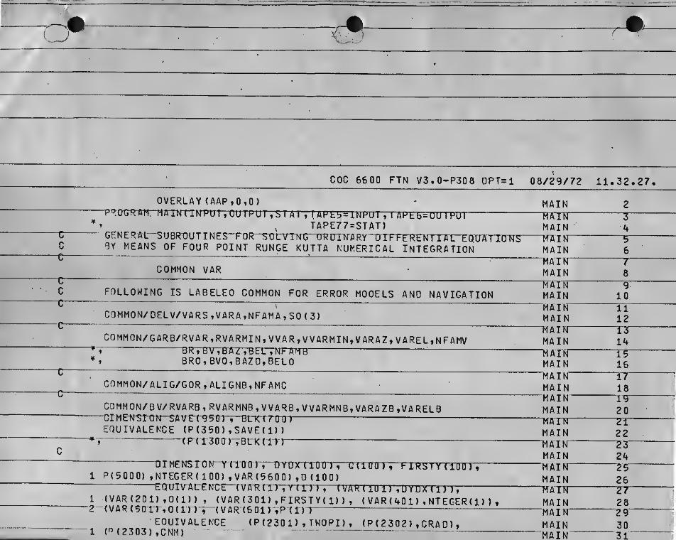
OVERLAY {AAP,0,0)PROGRAM. HAIN( IKPUT,OUTPIJTTSTAr,TAPt6 = iNPUT , T APhb=UU I PUI
,TAPE77 =STAT)— GFNERAL~SUeR-OUT I NES““rOR“S0CTmrG“"CrRirT'N
BY MEANS OF FOUR POINT RUNGE KUTTA NUMERICAL INTEGRATION
COMMON VAR
FOLLOWING IS LABELED COMMON FOR ERROR MODELS AND NAVIGATION
COMMON/ DEL V/ VARS, VAR A, NFAM A, SO (3)
COMMON/GARB/RVAR.RVARMIN, VV.AR,VVARMIN,VARAZ,VAREL,NFAMV•BRTBVVBA Z , BE L , NK AM B
'
8R0,BV0,BAZ0,BEL0
MAINTfATfTMAIN
:n“
MAIN"MAIN”MAINH'&IWMAIN"MAIN"MAINMAIN”'MAINMAIN-MAIN
c
—
COMMON/ ALIG/GDR,ALIGNB,NFAMC
COMMON/BV/RVARB, RVARMN8, VVARB, VVARMNB,VARAZB,VARELBuj.nc.fv:>iuiN iwvtiysui, OLNiruuT —EQUIVALENCE ( P (3 50 ) , S AVE ( 1 )
)
C,BLK(ir)
uintN^siU^ YtlUUJ, DTPXdUU), URSTYdOD)^1 P(5000) ,NTEGER( 100) , VAR (5600) ,D (100)
tatIIV'ALENCE“"(V/rRCT)l Yd')') , {VAR( lU i)‘,UYUX (1) ),
1 (VAR(2D1) ,Q(1)) , (VAR(301),FIRSTY(1)), ( VAR ( 40 1 ) , NTEGER (1) >
,
2 '(VARtSOirtOd) ) (VAR(601)-,P {1)T• EQUIVALENCE (P(2301) , TWOPI) , ( P ( 23 02) , CRAD >
,
1 (^(2303), CNM)- --
MAIMMAINMAINMAINTfATMMAINMAIMMAINMAIMMAINKAIMMAINMAIMMAINMAIN
2
-T4
~5-
6
-T8
“9101112TJ14TF16171819'
202T2273'
242526772829'
3031

DO 20 J=l,5600-0
SET IN FUNDAMENTAL CONSTANTSTWOPI=6V28?l 653072
—
CRA0=57. 2557795131: (rNH=6T}TBvrtl'333
LOA(T ERROR MODELVARS-ItE-4\/ARA = l,E-l
RVAR=Q,—RVAI^KT N 33.VVAR=4.3E-3V'/ARMIN = .43
VARAZ=2.E-3VAREL = 27E-3‘
99=0.3V=inBAZ=0.qel=d;—: '
—
n9o=o.ovo=o; ^ ^
BAZ0=17.45E-3
A MAINMAINMAINMAINSE NSORSENsOR^MAINMAINSENSOR'SENSOR'MAINTi'/aN
MAIN'MAINMAIN'MAIN
40TTI
42441
47
3
4
52
545557'58'
MAIN 59
CDC 6600 FTN V3.0-P3d 8 OPT=l 08/29/72 i1.32,27.
MAIN 60
MAIN 62“MAIN bJRANNO 1
RANNO 2RANNO 3
“RAXNT5MAIN 65SENSOR 5SENSOR 6
MAIN ^68‘

VARFLB=2,E-3.
SET OFRIVATIVE OF INDEPENDENT VARlAu^.OYDX(l)—
C| StI OF GTAS TERH5 EiuAt ZERC“0 0-35-T=Ti6DYDX(I + 13) = 0.
0Y0X(If31)=D.35 CONTINUE
c’—str JO >3 counterLOOP=0
s.
«o
Cf'
a
rs.
N.
ICO
eo

o
ifV
kD
Ni
i«0
O'
00
^CO
jOO
GO

•JEROUTIN. MMY2 CL.^600 FTN V3.0-P308 OPT=l 08/29/72 li.bZT27.
SUBROUTINE OUMMY2 . MAIN 90—c
CALL OVEPLAY(3HAAP,2,0,6HRECALL) MAIN 92RETURN MAIN 93END MAIN 94

r
‘U'
iek PrimaryO/PXS F
OVERLAY (1,0): PRULKAH NAVLAV
C TRANSFER CONTROL TO INTEGRATION(TALX—R KEND
. o600 FTN V3.0-P308 OPT=l 08/29/72 ll^i'

PROGRAM MAINAREA A
AREA B
ROUTINE RKAREA A
AREA B
AREA C
[
AREA D
AREA E
AREA F
THE PURPOSE AND HANDLING OF THESE INSTRUCTIONS IS DIS-
CUSSED IN SECTION 3.1
TIME DERIVATIVES OF BIAS PORTION OF INTEGRATED STATE
VECTORS IS SET EQUAL TO ZERO, ALL ESTIMATED SENSOR
BIASES ARE ASSUMED CONSTANT,
IF -THIS PASS THROUGH ^ IS A RETURN FROM THE GUIDANCE
OVERLAY, NOVER WILL BE SET TO 1,2,3 OR 4, DEPENDING
ON THE LOCATION IN GNEXEC WHICH CALLED THE OVERLAY, IN
THIS CASE, IT IS DESIRED TO GO DIRECTLY BACK TO GNEXEC ,
CALL TO SETY LOADS A CARTESIAN FORM OF THE BETELGEUSE
ESTIMATED STATE INTO Y(38) - Y(55) FOR USE BY OTHERSUBROUTINES. THIS MUST BE ACCOMPLISHED EACH INTEGRATIONSTEP BEFORE VISITING OUTPUT OR NAVIGATION EXECUTIVE,
CALL TO POPOUT ACCOMPLISHES COMPUTATION OF RELATIVESTATE QUANTITIES FOR USE BY NAVIGATION, AND PERIODICPRINTING OF BLOCK DATA DESCRIBED IN SECTION 4,0
GUIDANCE AND NAVIGATION IS VISITED EACH INTEGRATION CYCLETO PROVIDE FOR PERFORMANCE OF NAVIGATION, COMPUTATIONOF MANEUVERS AND MANEUVER APPLICATION
RK WILL BE CALLED PERIODICALLY AT ENTRY RKW FROM ADVWFOR ADVANCEMENT -OF COVARIANCE. IN THIS CASE, IT IS DESIREDTO GO TO THE RETURN STATEMENT AT THE CONCLUSION OF THESTATE INTEGRATION INSTRUCTIONS. BY SETTING NFLGW^l UPONENTRY AT RIOT, PROGRAM WILL RETURN TO CALLING ROUTINEADVW INSTEAD OF PROCEEDING TO NEXT INTEGRATION STEP.
FLAG IS RESET UPON NEXT NORMAL PASS THROUGH m,
LOGICAL OPERATOR TRANSFERS CONTROL TO RETURN STATEMENTIF NFLGW IS SET. OTHERWISE PLATFORM DRIFTS ARE INTE-GRATED ONE STEP BEFORE GOING ON TO NEXT PASS THROUGH RK.
17
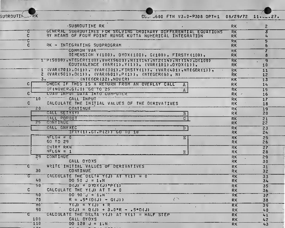
SUeROUTlK. CL- o600 FTN V3.0-P308 OPT=l 08/29/72 ll.w^.27.
'SUBROUTINE RK
BY MEANS OF FOUR' POINT RUNGE KUTTA NUMERICAL INTEGRATION
RK - INTEGRATING SUBPROGRAMCOMMON VAR~~~ ^
DIMENSION YdOO), DYOX(IOQ), GdOO), FIRSTY<100),I—PTBOOCl) ,NTEGERTT[nrrTTrAR(56UU) ,NUd4J ,'NT2(14) ,NT (ID ,D(
EQUIVALENCE ( VA R ( 1 ) , Y ( 1 ) ) , ( VAR ( 10 1 ) ,0 YO X d ) )
,
1 (VAR , Qd) ) ," (VAR (3 01) ,'riRSTY dTTr”( VAR CAOinNTEGERTr
2 {VAR(501) ,0( 1) ) , (VARCeOi) ,P d) ) , (NTEGERCB), N)
3,- - -
• (NTEGER(32) ,NOVER)
IMIlilUIBISA
“INPUTE INITIAL VALUES OF THE DERIVATIVESinue'
"
1 CALL POPQUT Cl—7F CONTINUE
1CALL GNEXEC D
1L —ih (Yd)' ruTTvrzT ) LU lU lU
NFLGW = 0
GO TO 29E
'
’ENTRY' RKW“'NFLGW = 1 ECONTINUE
CALL OYOXSWRITE INITIAL" VALUES“OF“DERrVA‘T IVES
CONTINUECATCUIIAT E“'THE"0‘ErTA Y(J) AT Yd)
00 50 J = ItND (U) = D YDXTJ )^PTT)
CALCULATE THE Y(J) AT T = 0
00 90" j-'=“r,N-R = .5* (0(J) - Q( J)
)
Q(J) = Q (J) +
'CAUC'OLATETH E^TL'TA~YTCALL OYOXS00 120 J = 1,N
3.0*R - .5»n(J)
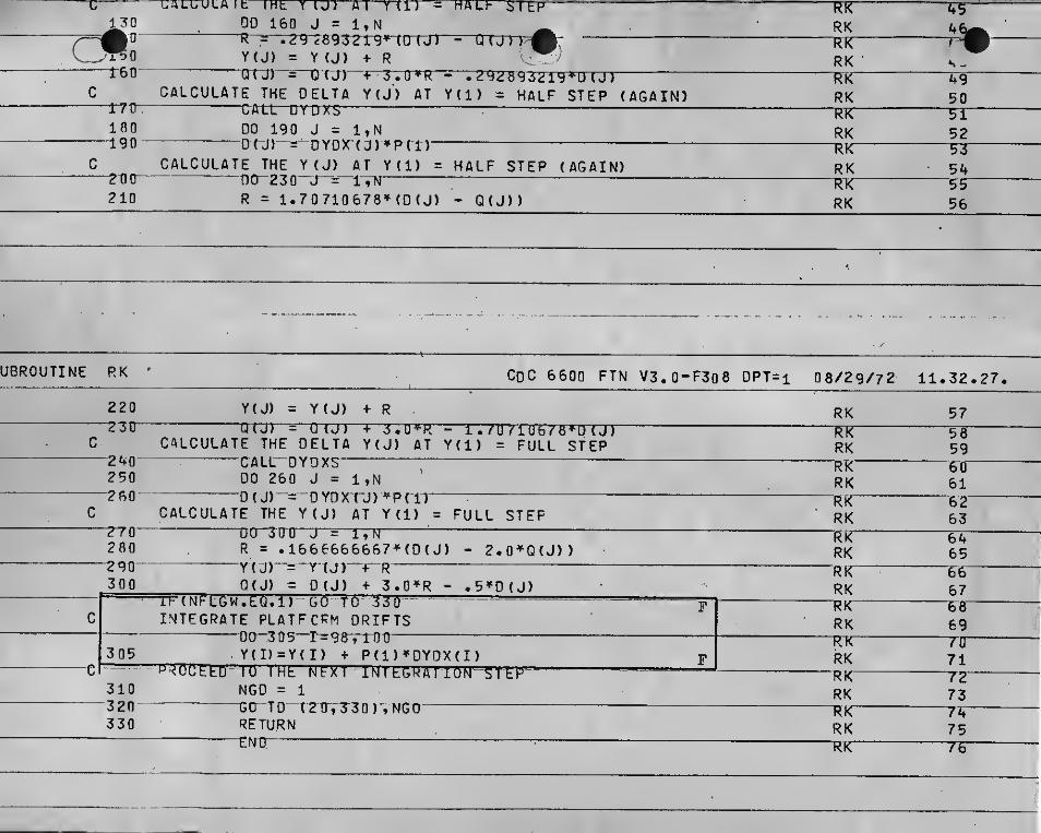
00 160 J = 1,NR~^ >29Tg^7er9»tU (J)
~Q
Y(J) = Y (J) + R^OTJ) OTzn—+~3V0 R • 2
CALCULATE THE DELTA Y(J) AT Y(l) = HALF STEP (AGAIN)
00 190 J = 1,N0( j)-="'OYDr(a)*FnD
CALCULATE THE Y(J) AT Y(l) = HALF STEP (AGAIN)••
nO"230“‘J~=~lV>JR = 1.70710678*(D(J) - Q(J))
UBROUTINE RK
220
CoC 6600 FTN V3.0-F308 OPT=i 08/29/72 11.32.27
Y(J) = Y(J) + R

TAJpur

ROUTTOE INPUTAREA. A FIRST TWO INSTRUCTIONS CHECK N¥(l) ARRAY (SEE SEC 3 . 2 )
TO RESET W-MATRIX REINITIALIZATION FLAGS. IF ANY FLAG' OF THIS ARRAY IS 0 ON INPUT NAVIGATION CONTROL CARD, IT
IS SET TO -1 AT TBIE W IS REINITIALIZED. LAST FOUR IN-
STRUCTIONS IN THIS ARE WRITE OUT ACCUMULATED MONTE-CARLODATA TO LOCAL MASS STORAGE FILE AND THEN ZERO ARRAY FORNEXT CYCLE.
AREA B AT BEGINNING OF PROGRAM EXECUTION, SYSTEM ROUTINES AREREAD TO DETERMINE DATE AND TIME OF THIS RUN. THIS IN-
FORMATION PLUS THE NUMBER OF MONTE-CARLO CYCLES TO BEEXECUTED ARE THE READ ONTO BEGINNING OF MASS STORAGEFILE.
AREA C FOLLOWING INPUT OF BSTELGEUSE HOLLERITH COMMENT CARDS,
A CARD SPECIFYING THE MANEUVERS AT WHICH DATA WILL BESTORED IS READ IN AND PRINTED OUT. NO MORE THAN 8 ELE-MENTS OF NST(l) MAY BE NON-ZERO; THE DATA ARRAY HAS
ROOM FOR ONLY 8 MANEUVERS WORTH OF DATA.
AREA D AETER INFUT OF BETELGEUSE FLOATING POINT ENTRIES, ASERIES OF UP TO 10 NAVIGATION CONTROL CARDS IS READ IN,
NUMBER OF THESE CARDS IS EQUAL TO NPER . AITER INPUT,
TIME, LENGTH, AND ANGLE QUANTITIES ARE RESCALED TO FUNDA-MENTAL UNITS OF SECONDS, FEET AND RADIANS,
AREA E FOLLOWING NAVIGATION CONTROL CARDS, AN ALIGNMENT CONTROLCARD, AS SPECIFIED IN SEC 3.2 IS READ AND ALIGNMENT TIMESPRINTED OUT.
AREA F DATA ARRAY STACK INDEX IS RESET, THIS INDEX IS INCREMENTED
BY 1 EACH TIME A 31 ELEMENT ARRAY OF VECTOR AND MANEUVERDATA IS STORED IN THE DATA ARRAY. SEE MASS DATA STORAGE,PAGE 9.
AREA G RESET MANEUVER TYPE COMPUTATION FLAG TO STARTING VALUE.RESET ALIGNMENT COUNTER FLAG (INCREMEWTED BY 1 EACH TIME
AN ALIGNMENT IS PERFORMED,SET MANEUVER COMPUTATION FLAG TO CALL FOR AN INITIALVISIT TO THE GUIDANCE OVERLAY AT FIRST VISIT TO GNEXEC.
AREA H ZERO THE W-MATRIX TO BE SURE ITS NICE AND CLEAN FOR NEXTCYCLE.LOAD ESTIMATED CARTESIAN STATE INTO Y(38)-Y(55).PERFORM INITIAL ALIGNMENT TO DEFINE PLATFORM AXES.
18
?OUTIN^-^INPUT o600 FTN V3.0-P308 OPT=:i 08/29/72 11.0-^27
SUB-ROUTINE INPUTiza
BY MEANS OF FOUR. POINT RUNGE KUTTA NUMERICAL INTEGRATION
INPUT - SUBPROGRAM FOR READING IN DATACOMM ON “VARDIMENSION Y(IOQ), DYOX(IOD), Q(IOO), FIRSTYdOO),
ir-P ( 5tl-fm-TWrEGERtT00 ) t VAR ( 56 0 0 ) ,NrnT4-
T , N T 2 ( 14 ) ^ N T 1 14 ) , Dn ai
EQUIVALENCE ( VAR ( 1) , Y ( 1) ) , ( V AR ( 10 1 ) ,0 YDX ( 1 ) )
,
-l-tVARteOl) ,0(1)) ,“(VAR(30l)-,FIRSTY(TVrr'XVAR-{41inTNTFGERTi:2 (VAP (501) ,0(1) ) , (VAR(601> ,P (1) ) , (NTEGER( 6) ,N)
,
-3 • (NTEGER-( l) ,IOEN T )",' (NTEGER ( 2) ,-NP)-;—(NTEGER (3T, NINTII
4 (NTEGER(4) ,NFIRST) , ( NTEGER ( 5 ) , NT A BLE )
,
(NTEGER(7) ,NM0RE)-5—(NTEGFRr8.r-,NT(t- ) ) ,
' (-NTEGERt^TTTNTCR ) , CrnTGETRI 2 Vj tN'TSKIFT'6 (NTEGER(41) ,LPRINT) , (NTEGFR (42) ,NLINE)
,
(NTEGER(43) ,NSKI17- (NTEr,ER(44),NPAGEr-,~(NTHGER (Vs ) VNT 1( ir)-,-“(NTEGER (60 )‘VNT2 (
DIMENSION NST(i5), TIG(15)EQUIVALFNCE"(P(294) •iNFAM2)
(NTEGER(43) ,NSKIP)
,
(NTEGER(60)VNT2(rrr
(P(295) ,L00P)(PI-3 34-1-rNST-AT1
(P(335) ,NST (1)
)
(P(2107) vTTPI) -T(P(2141) ,TIG(1)
)
E 0 U I V-AtE’Nt^E- ( N T E GE R ( 1 2 ) NPER )
(NTEGER(29) ,NGUIOE)( N T-eGffm-o )-;-ictm-p)
. (NTEGER(33) ,LIGN)(NT EGER {-35)-,NGA-TE)
(NTEGER (36) ,NBRFL)6lMENS-rtlN-SAVE(950)~rBLK(700 )~, D A T A (
EQUIVALENCE (P ( 350 ), SAVE ( 1) )
TFTr? O CHTBCK T IT")
(P(4074) ,DATA(1)
)
“ — (p-( 4 V Cl tTilDIMENSION QQ(4), SIG(4), C(IO), REFM
ZNBN(3),' 'NE(IO) NM(IO) , 0USP(IQ), USV(IO) , UTP(IO)
,
SOTm"," ' SCrRTDT7"“SCE'( 10 )
,
ZTZ(4) , S7(4) , TALIGN(IO)
,
X(18) , WE{18,27)EQUIVALENCE (S A V E ( 1 ) , QQ ( 1 ) )
,
••
(SAVr(9) ,C(1) ) ,
REFMAT(3,3), XN8N(3), YNBN(3)
UTVdO) , SRdO) , SRDCIO)
XNBE(3), YNBE(3), ZNBE(3)
(SAVE(5) ,SIGd) )
(SAVE (19) ,REFMAT(i,l) )'
INPUT
X lY r w t
INPUTTNPirrINPUTINPUT”INPUTINP'OT"INPUTINPyT"INPUT"INPUT"INPUTTKPcrrINPUT"INPUT-INPUT"INPUT-INPUTTNPOINPUT"INPUT-
INPUT"INPUrINPUT
"TT4P
INPUTINPUTINPUT"INPUTINPUTTRPTrrINPUT^NPUTINPUT‘INPUTINPUT_“ N'inrrINPUTINPUTINPUTINPUT

(SAVF(47) ,NM(1) ) ,
vt to r J f IMt 11 J I
i^AVE (57) ,0TL(1))iNKUlINPUT
4t>
46^^1# ’ rsnvf(6/) , DTNTm
,
T^iVe (77) ,“DTM( 1)
)
INPUT ^ w(SAVE(87) ,USP{1) )
,
^ xoAVE (97) ,USV(1)) INPUT 4w^ rsAVErTrcr7TTUTP'( rrn rS'AVE (117 ) fUTV (D) INPUT 49
^ , (SAVE(127) ,SR(1) )
,
(SAVE (137) ,SRDtl)) INPUT 50— 1 III im imra^M INPUT 51(SAVE(167.) ,SC2 (1) ) , (SAVE (177) ,NW(1)) INPUT 52(SAvrdBDvTLMcrrn TSAVETl^TT^N'S (TT) I'M PUT 53(SAVE(20Q) ,ZT2(1) ) (SAVE (204) ,SZ(1)) INPUT 54tSAvt<2Ub)» !ALibN(i)^j (bAvt (i^lo))riiALibNj INPUT 55(SAVE(229) , XNBE(l) )
,
(SAV£(232 ) ,YNBE (1) ) INPUT 56
i
JePOUTINE INPUT COC1
6600 FTN V3,0-P308 OPT=l 08/29/72 11. 32,27.
V-, (SAVE(235) ,ZNBE(1) ) , (SAVE(258) ,X(1) ) INPUT 57HMM—
—
INPUT 56c ZERO THE WORKING ARRAYS INPUT 59
INPUT 605 RLK(I)=Q. INPUT 61
CT" SET~T^Gir'NO -QF^nRST PAGE INPUT 6210 NPAGE = 1 INPUT 63
L-'JUP = LUOP + 1^
64TF(LCOP.EQ.l) GO TO 20 INPUT 65
* OO'll 1=1,10“
A 6611 IF<NW(I) .LT.O) NW(I) =0 INPUT 67
WR I TE ( 7 7) to AT-A'I'T)’ , I'^ ,351}')
“INPUT 68
CALL OUTOAT INPUT 6900 lr5 1 = 1, I'NPTn
15 OATA(I)=0. A INPUT 71IF ( L c1TP.“G T •- 1 0E N T ) G U -
! 0 2 O'^
INPUT 7^2
WRITE (6, 80) INPUT 73GO ( u 3o 0 INPUT 74
C READ CONTROL. INTEGERS INTO PROBLEM INPUT 75Etn XOOP = l INPUT 76
REAO(5,30) (NTEGER(J),J=1,14) INPUT 77—CT" MAKE' END-0F-FILE“CHFCK INPUT 78. IF(EOF(5)) 21, 22 INPUT 79
21 CALL EXIT- INPUT 80r> n Ilpt t m I I it
lUUU FORMA raHU,i4X*39H»* DATA INPUT T'lJlTTHIS RUN ^*//i8X;INPUT
r m ' wa u ’OA'rr;" TTMF ANU ^IZE 'OF’ 'UPUU'M'ING bl AI TSI ICAL Sbl BCALL DATE(IDATE) ^
INPUTINPUT
82
p—- (
#i
CALL'TIMEdTIMEr*^ “~WWRITE (77) IDATEdTIMEdOFNT B
INPUTINPUT
^ •3040
F0RMAT(1AI5)IF (NMOR,E)60,60,50
INPUTINPUT
8687
“5T] NMO = 14 +"NMORt INPUT 88READ (5, 30) (NTEGER(J) ,J=15,NMO) INPUT 89
cr WRtTEr~HrAOING A T TOP' ‘Or“P AGE™ INPUT 9060 CONTINUE INPUT 91
NLINE=3a™ '
INPUT 92c READ AND WRITE TWO CARDS OF RUN INFORMATION INPUT 93
RLAU (b, BU) INPUT 9400 FORMAT {72H INPUT 95
1....
INPUT 962 ) II^PUT 97
. ^ INPUT 98WRITE(6, 1000) INPUT 99
101(T READ CONTROL'TLAGS'TOR'IIArA* 3TOR1AGE
READ 475, (NST( I) ,1=1,15)C INPUT
INPUT102103
475PRINr-480, [NSTTT")"^t=XiI5')FORMAT(15I5)
104105
4"50*
RDRWATT7Dr75THBirCCTrTrAT A WILL B E 'S T aRED'""AT rHE",1515)
FOLLOWINflC
NGUIDES- INPUTINPUT
106107
: ^100
CHECK FOR INDIVTDUAL -FLOATJNG^(JINT~inrrA*'HNTRY“IF[NP)2E0,250,110
INPUTINPUT
106109
1*10"' DO 140'“J'"="TVNPREAD(.5,130) I,P(I)
INPUTINPUT
110111
UBROUTINE INPUT COC 6600 FTN V3,0-P308 OPT=l 08/29/72 11.32.27.
130 F0RHAT(I5,£15.7) INPUT 112WRI IE (6,1001) ITPTT) Input 113
1001 FORMAT(17X,I5,3X,Ei5.8) INPUT 1141^0 CONTINUE INPUT 115
IF{NTEGER(13) .GT.O) WRITE ( 6» 10 03 ) INPUT 116FORMAT (//20X, INPUT 117'10 03

tL AJNTUI AX'S3 20X,19H*» THAT THIS RUN **/ INPUT WKBffA-
4
20X>1-9H’^» W A S“M A 0Em N »»7 IN P UT 121”5 20X,19H^* AN OBLATE **/ V. INPUT IL
6 — 20Xvr9H*»—ENVIRONMENT ^ INPUT IPT7
,INPUT 129
8
2tJ XtI'9 ITTPTJT TE?’
C INPUT 126C CHECK IF NAVIGATION DATA IS INmNPUTmiLE D
IF (NPER.EQ.O) GO TO 155INPUT ^127
INPUT 128- C READ ANO'SCALE NAVIGATION" OATA'-'^
DO 145 I=1,NPERINPUT 129INPUT 130
- RE A0F5-, TOtTAT NmiyNM mTOTL ( 1 ) , U 1 N ( 1 ) ,U 1 M 1 1 » , USP ( 1 ) ,US\
1 ,UTP{ I) , UTV (I) ,SR (I) ,SRD (I) ,SO(I) , SCI ( I) , SC2 ( I
)
Tn TRPUT 131INPUT 132— 2,NW(T) -
PRINT 460,NE( I) ,NM(I) ,OTL (I) ,OTN(I) ,OTM(I) ,USP(I) ,USV(IINPUT 133INPUT 134
i,uTP(T) vuTV(ir,sRTi)vsRDmTsam“,sciTT) isozui ^may460 F0RMAT(/1X»134H NE NM DTL OTN DTM
INPUT 135USP INPUT 136
y-- USV~‘
OTP UPV SR SRD2 SCI SC2 NW ,/lX»2I5,3F10.1,9F10 .2,13)
SO INPUT 137INPUT 138
C SCALE DATA ^DTL(T)=DTL(I)'^60.
INPUT 139INPUT 140
“ GTN(I) = nTN(I)“^60. ^
DrM(I) = OTM (I)»6a
.
INPUT 141INPUT 142
usH (r)=usp(i)»iaoo.UTP{I) = UTP(I)V100Q.
INPUT 143INPUT 144
SR(I1 =SR(I)’^in00 .
so (T)=SO(I)/1000 .'
INPUT 145INPUT 146
.trov F0RMAT(2I2,3F7. 1,'9F5,2,I2),145 CONTINUE D
INPUT 147INPUT 148
R F A n "1 0 0 5V NAm G N ^ fT AVI GN fDTI = 1 , N A L t G N ) EL0Q5 FORMAT(I2,10E7.1)
INPUT 149INPUT 150
‘ I'^CNALIGNVLT.l)- GO' TCTTSOPRINT 465, NALIGN
INPUT 151INPUT' 152
no 146 i=iInalignAT^= miNPUT 153
INPUT 154TAB PRINT-ATU, VALIGNd)470 FORMAT(/44X,F10.1)
TNPXrT 15?INPUT 156
150 CONTINUEj55 continue E
INPUT 157INPUT 158
X' :- - -
INPUT ^159
ICON INPUT 16DNFflM2 = P'C297) rNPUT 1^
C CHECK IF COVARIANCE MATRIX IS TO BE READ IN INPUT 162TF{NFAM2r~24irr2R07‘2^nJ INPUT 163
240 CALL INPUTD . INPUT 164-Q CHECK' IF TABLE"FNTRXES"ARr"TO"BEnnS0T INPUT 165

.-Mr-NTl(l) = NTCR
, ^ INPUT 167^rjo 370 M = 1,NI A4Lb. 7^9 msiiiflH
2 80 IF(NT(M))290 ,370,310 v,- INPUT IL^ NTT CM -FT) =“RTrTKT INPUT
GO TO 370 • INPUT 171NTKM+IT = NTHMT“TnmTn INPUT 172
320 NT2(M) = NTl (M) «1 + NT (M) INPUT 173NTT1““= NTTTRT INPUT 174NT12 = NT2{M) INPUT 175KtAU(t>t3bU) 1 H 1 » J= N I 1 1 * N 1 12 > INPUT 176
360 FORMAT(7F10.7) INPUT 1773 ^ U CONTINU E INPUT 176
c CALL INPUT WRITECUT AND IC CALC ROUTINE INPUT 1793 11 CAim N ATO ^^1i *
1 11MM MKnMI^^BMc SET MANEUVER COMPUTATION FLAG INPUT 181
’=*( 1 0) =- CP (9) + 1 •) INPUT 182NS 1 A 1 = LI
^
F INPUT 183UA 1 A C 1) =LUUM INPUT 184DATA (321) = NFAM2 INPUT 185PRINT" 45D, P {'2T INPUT 186
450 FORMAT (/1X,5HP (2 ) EIE.S) INPUT 187NGUIOE = Nfe’CER(3) G ^^^Mi1 flUliMB 188LIGN=0 INPUT 189ICOMP=l 'G' INPUT 190
c S'-T TPI TIME INTO" erasable INPUT 191IIb(5)=llPi
, INPUT 192c SET 9RAKING GATE INDEX TO FIRST GATE INPUT 193
Nb A 1 t-
1
INPUT 194c SET BRAKING FLAG TO ZERO INPUT 195
NBRFL = 0 INPUT 196c ZERO THE Q AND SET IN IC INPUT 197
mnim DO 420' J" ="T,
N
INPUT 198Q 9 0(J) = 0.0 INPUT 199^EiH orCJ) = FTRSTTTJV INPUT 200ISslil CONTINUE INPUT 201
c /EPO THE WE MATRIX H INPUT 202DO 421 1=1,18 INPUT 203Ou 421 J— 1,^/* TNP O'T 2d4WECItJ) = 0.0 INPUT 205
421 CONT INUE INPUT 2 06c SET UP VECTORS AND PERFORM INITIAL ALIGNMENT INPUT 207
CALL SETY(T) INPUT 208CALL ALIGN H INPUT 209
c construct EffUTRCTTME NT VhCi'OR Tfmn—425 CALL ICfRR INPUT430 RETURN "
'
^ INPUT 212ki r\

ROUTINE (2TEXEC
area a • GUIDAECE OVERLAY RETURE CHECK. IF NOVER FLAG IS OTHER
THAN ZERO, GNEXEC HAS BEEN CALLED ON RETURN FROM THE
GUIDANCE OVERLAY. VALUE OF NOVER (1,2, 3, 4) INDICATES
ELACE IN GNEXEC WHICH CALLED GUIDANCE OVERLAY. EXECU-
: ) TION OF THE GO TO STATEMENT RETURNS CONTROL TO STATE-
MpT FOLLOWING ONE THAT CALLED OVERLAY.
AREA B LIGN FLAG IS INCREMENTED EACH TIME A PLATFORM ALIGN-
MENT IS PERFORMED, CHECK IS MADE TO DETERMINE IF LIGN
IS EQUAL TO NUMBER OF ALIGNMENTS SCHEDULED ON INPUT.
CHECK IS THEN MADE TO SEE IF THE NEXT ALIGN IS LESS
THAN ONE INTEGRATION STEP AWAY.
AREA C IF NO NAVIGATION PROCEDURE CARDS WERE READ IN ON IN-
PUT, CONTROL IS TRANSFERRED OUT OF THE NAVIGATION
CONTROL PORTION,
AREA D BEGIN DO LOOP WHICH CYCLES THROUGH THE NAVIGATION
CONTROL CARDS READ IN ON INPUT. IF CARD IS NOT AC-
TIVE, LOOP TURNS TO NEXT CARD.
area E if card IS ACTIVE FOR THIS NGUIDE (NE(I)j^O), CHECK IS
MADE TO SEE IF A SENSOR IS ON. IF SENSOR IS OFF, CON-
TROL IS TRANSFERRED TO W-MATRIX INITIALIZATION SECTION
TO SEE IF THIS CARD IS PRESENT ONLY TO RESET W.
AREA F IF FIRST RENDEZVOUS MANEUVER IS NCI, TIME SINCE LAST
MANEUVER IS DEFINED AS PROGRAM ELAPSED TIME. OTHERWISE,
PROGRAM ELAPSED TIME MINUS PREVIOUS TIG.
AREA G TIME TO NEXT MANEUVER IS TIG FOR CURRENT MANEUVER MINUS
PROGRAM ELAPSED TIME.
AREA H SEE IF TIME SINCE LAST MANEUVER IS GREATER THAN MINIMUM
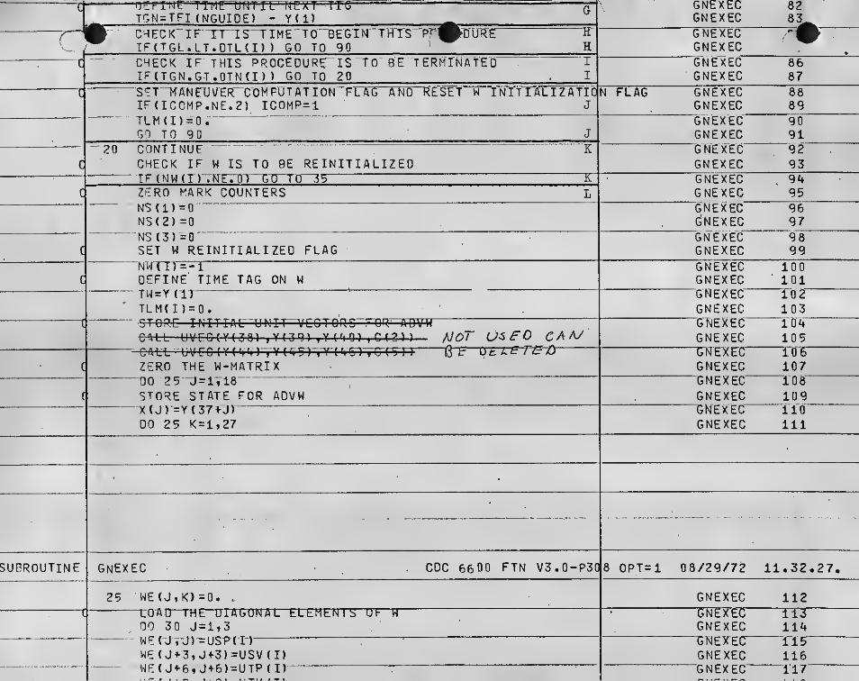
TIME TO BEGIN THIS PROCEDURE,
AREA I SEE IF TIME TO NEXT MANEUVER IS STILL GREATER THAN
MINIMUM TIME TO TERMINATE BEFORE MANEUVER.
AREA J IF IT IS TIME TO TERMINATE THIS PROCEDURE, MANEUVER
COMPUTATION FLAG IS SET = 1 TO INDICATE A MARKING PRO-
CEDURE HAS TERMINATED AND THE GUIDANCE CONTROL SECTION
CAN CALL THE GUIDANCE OVERLAY TO COMHJTE A BURN.
TIME SINCE LAST MARK ON THIS PROCEDURE IS SET TO ZERO
FOR NEXT CYCLE ON MONTE-CARLO SET.
AREA K CHECK TO SEE IF THIS PROCEDURE CALLS FOR W TO BE RESET.
OTHERWISE GO DIRECTLY TO MARKING SECTION AREAS M-P.
19

area l reinitialize W:
SET SENSOR MARK COUNTERS TO ZERO. •
• SET THE CARD INITIALIZATION FLAG TO -1 INDICATING FOR
FUTURE PASSES THAT REINITIALIZATION HAS BEEN DONE. THIS
flag will be reset in input ON BEGBINING NEXT MONTE-CARLO
CYCLE. _DEFINE TIME TAG ON W AS CURRENT ELAPSED PROGRAM TIME,
SET TIME OF LAST MARK ON THIS PROCEDURE EQUAL 0.
STORE THE CURRENT CARTESIAN ESTIMATED STATE FOR THE
W-MATRIX ADVANCEMENT ROUTINE, ZERO OUT ELEMENTS OF W.
CALL FOR BLOCK PRINT AT THE REINITIALIZATION.
area M IF SENSORS WERE OFF AND THIS CARD IS ONLY TO RESET W,
TURN TO NEXT CARD.
area N DEFINE THE TIME INTERVAL SINCE LAST MARK ON THIS PRO-
CEDURE AS PROGRAM ELAPSED TIME MINUS TIME OF LAST MARK.
AREA 0 SINCE MARKING IS ABOUT TO TAKE PLACE, MANEUVER COMPU-
TATION FLAG IS RESET TO INDICATE THAT ESTIMATED STATE
IS GOING TO BE UPDATED AND A NEW MANEUVER COMPUTATION
WILL BE NECESSARY.
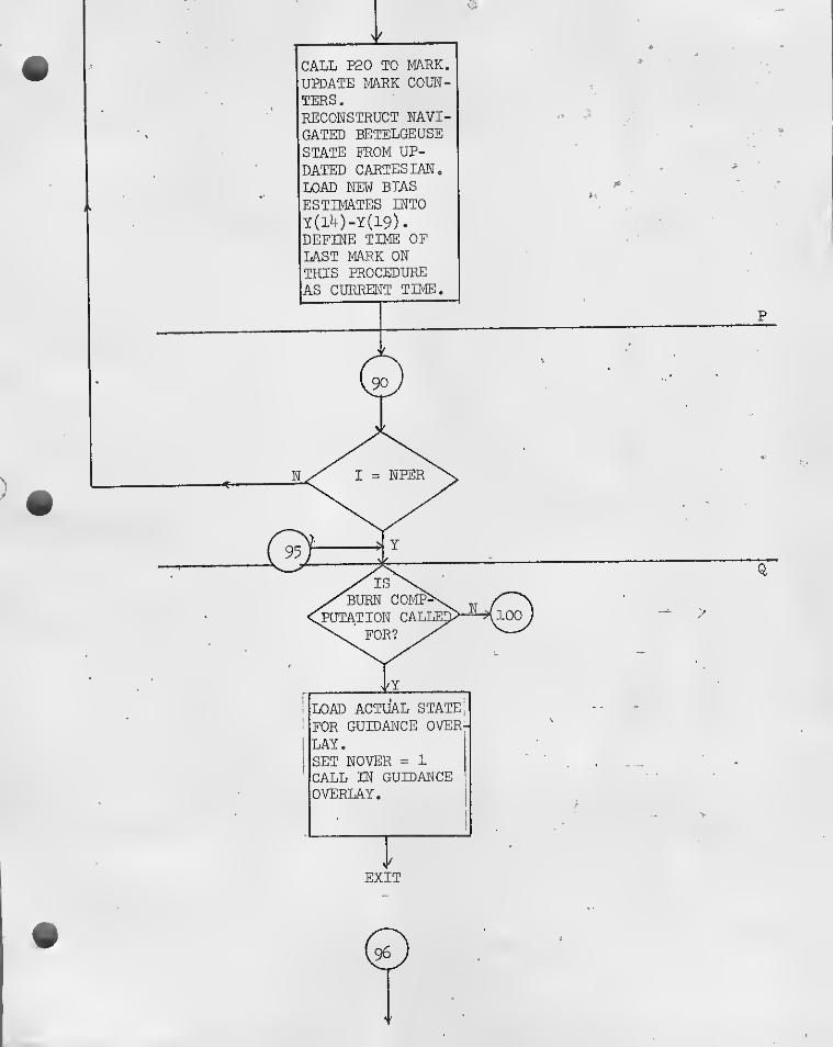
AREA P TAKING A MARK:CHECK IF TIME SINCE LAST MARK IS GREATER THAN MINIMUM
ALLOWED TIME BETWEEN MARKS ON THIS PROCEDURE, IF NOT,
TURN TO NEXT CARD.
CALL P20 WITH CURRENT TIME, CURRENT ESTIMATED CARTESIAN
STATE, AND SENSOR TYPE FLAG.
UPDATE THE MARK -COUNTER. THE NM(I)=4 OPTION IS A LATE
ADDITION COMBINING A RANGE AND OPTICS MARK, FOR THIS
OPTION, BOTH THE RANGE AND OPTICS MARK COUNTERS ARE
INCREMENTED-.SINCE THE CARTESIAN ESTIMATED STATE IS NOW UPDATED, IT
IS NECESSARY TO RECONSTRUCT THE BETELGEUSE ESTIMATED
STATE FOR INTEGRATION BY RK .
TRANSFER REVISED ESTIMATES OF SENSOR BIASES TO BETEL-
GEUSE ESTIMATED VECTOR,
DEFINE TIME OF LAST MARK ON THIS PROCEDURE AS CURRENT
PROGRAM TIME.
AREA Q IF A MARKING PROCEEDURE HAS JUST TERMINATED ,THE ICOMP
FLAG IS EQUAL 1. IN THIS CASE, AREA Q COMPUTES A MANEU-
VER BASED ON THE VALUE OF NGUIDE, ONCE FOR THE ACTUAL
STATES AND ONCE FOR THE ESTIMATED. IF ICOMI^l, CONTROL
IS TRANSFERRED TO THE MANEUVER APPLICATION AREA (r) TO
SEE IF IT IS TIME FOR A MANEUVER.
COMPUTE A MANEUVER (RECYCLE OR FINAL)
'load actual BETELGEUSE STATS INTO GUIDANCE OVERLAY LO-
CATIONS
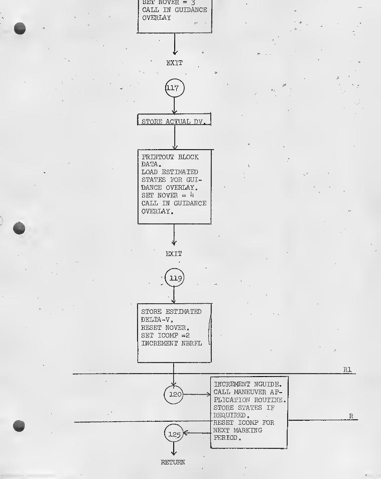
O 20

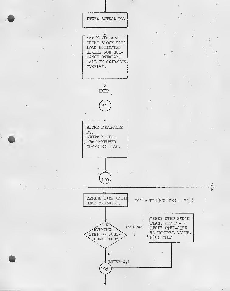
area. Q set overlay RETURN ErAG(NOVER) TO.l.
CALL GUIDANCE OVERLAYCALL STOREl TO STORE ACTUAL DELTAV. (CALLS TO THE STORE
RESULT IN STORAGE OF INFORMATION ONLY IF NST(NGUIDE)=1
(SEE PAGE 5 ,CARD #4)).
CALL FOR BLOCK PRINT AT MANEUVER COMPUTATION.
SET OVERLAY RETURN FLAG, N0VER=2.
LOAD ESTIMATED STATES.
CALL GUIDANCE OVERLAY.
CALL ST0RE2 TO STORE ESTIMATED DELTAV.
RESET OVERLAY RETURN FLAG.
SET IC0MP=2 TO ADVERTISE THAT A MANEUVER HAS BEEN COM-
PUTED AND IS AVAILABLE.
L
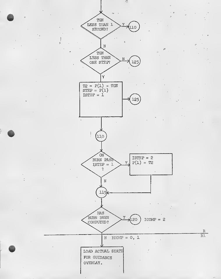
AREA R COMPUTE TIME TO GO UNTIL IGNITION.
SEE IF TC2I IS LESS THAN 1 SECOND, IF IT IS, GO TO AREA R1
TO CALCULATE A MANEUVER IF THIS IS NOT ALREADY DONE
,
IF TGN IS GREATER THAN 1 SECOND, SEE IF IT IS LESS THAN
ONE INTEGRATION STEP, IF NOT, EXIT ROUTINE.
IF TGN IS LESS THAN 1 INTEGRATION STEP, SAVE THE DIF-
FERENCE BETWEEN T(X^ AND STEP FOR USE ON THE NEXT (SYNCH)
PASS AFTER THE MANEUVER APPLICATION.
ALSO SAVE THE NOMINAL STEP SIZE.
DEFINE NEXT INTEGRATION STEP SIZE AS EQUAL TGN.
SET STEP SYNCH FLAG (lSTEP=l).
EXIT ROUTINE.
AREA RO ON NEXT PASS AFTER ONE ON WHICH TC2J WAS LESS THAN STEP,
TGN WILL BE ZERO. AREA RO IS THEN VISITED AS A RESULT OP
THE INSTRUCTION WHICH ASKS IF T(3J IS LESS THAN 1 SECOND.
STEP SYNCH FLAG IS INCREMENTED TO INDICATE NEXT PASS IS
•EVENING' STEP.
P(l) SET EQUAL TO T2
AREA R1 CHECK IS MADE TO SEE IF MANEUVER HAS BEEN COMPUTED . IF
SO, PROCEED DIRECTLY TO APPLICATION INSTRUCTIONS,
IF MAl^EUVER HAS NOT BEEN DEFINED, SEQUENCE OF COMPU-
TATIONAL INSTRUCTIONS IS PERFORMED IDENTICAL TO AREA Q.
AREA R2 INCREMENT NGUIDECALL DELTAV APPLICATION ROUTINE.
STORE STATES AT MANEUVEREXIT ROUTINE.
o21

yTEIS CAED\ACTIVE DUEIEC\THIS PERIQB'
CHECKING Ith NAV .PROCEDURE CARD
?HIS SENSO^ON?
EJ 20
CALCULATE TIME IN-
TERVAL SINCE LASTMANEUVER
CALCULATE TIMEINTERVAL UNTILNEXT MANEUVER
isX^XlT TIMETO BEGIN THISXvEROCEDURS^
ISX./^T TIME ^^0 STOP THIS
PROCEDURE'
N J 20
WQ
BO

w-MATRIX TO BE
\ RESET? ^
/is\“THIS SEN-SOR ON?
ZERO MARK COUNTERS.SET REINITIALIZATIONELAO TO -1.
SET TAG ON W EQUALTO CURRENT TIME,SET TIME OF LAST'MARK EQUAL ZERO.LOAD CURRENT ESTI-MATED CARTESIANSTATE FOR W-MATRIXADVANCEMENT AND ZEROTHE MATRIX.LOAD DIAGONAL ELE-MENTS OF W.
.CALL OUTPUT.
)
CALL P20 TO MARK.UPDATE MARK COUN-TERS.RECONSTRUCT NAVI-GATED BETELGEUSESTATE EROM UP-DATED CARTESIAN.
LOAD NEW BIASESTIMATES INTO
Y(14)-Y(19).DEFINE TIME OFLAST MARK ONTHIS PROCEDUREAS CURRENT TIME.
; LOAD ACTUAL STATE'
FOR GUIDANCE OVER-
ILAY.
i
SET NOVER = 1
CALL IN GUIDANCE:
OVERLAY.I
(
j
EXIT
*•
P
EXIT
SET NOVER = 3CALL m GUIDANCEOVERLAY
' f
EXIT
EXIT
RETUM

SUBROUTINE GNEXEC GNEXEC
SUBROUTINE TO CONTROL THE EXECUTION OF NAVIGATION PROCEDURES,GU 10 ANCE~C OMPUrATTO NS~ANu mATTEUVEr ApPLIUA r iUNS
COMMON- VARDIMENSION VAR(56aO), Y(IOO), DYDXClOO), Q(IOO), FIRSTY(IOO)
NTEGER-inrU) , U(IUU), P(bUUU)EOUIVALENCE (VAR(1),Y(1))
CVAR (101T,DYDX“(I1
1
(VAR(?01) ,Q(1)
)
“(VAR(301)',FTRSTYar)“^tVAR(LOl) ,NTEGER(1)
)
1 V AR-C5 0 m'o-irn :
(VAR(601> ,P(1)
)
G T MENS 1 0 N“SA VE(950),BLK(700 1 -,-CrAT^3 5 0 ) , COV(24, 2-r)
EQUIVALENCE (P (3 50 ) ,S AVE ( 1 )
)
(P( 1300) ,BLK( 1) )—'
(P(4074) ,DATA (1)
)
j p j
DIMENSION OQ(4), SIG(4), CdO), REFMAT(3,3), XNBN{3), YNBN(3)ZNBN ( 3 ) , NE (10), NM mnT'“DTrmn , DTN("iDivTrr>rrnn
—
USP(IO), USV(IO), UTP(IO), UTV(iO), SR(IO), SRD(l.O)SO ( 10 vvsci (10) 7 ‘SC^{la)”W(lInT^X'H‘(l(^^7^sl3)ZTZ(4), SZ(4), TALIGN(IO), XNBE(3), YNBE(3), ZN8E(3))f(18)i-REm8-,-27)'
EQUIVALENCE ( SA V E ( 1 ) , QQ ( 1 ) )
,
^ (SAVE(9) VC(T) )>
(SAVE(28) ,XN8N(1) )
,
(SAVE(34) ,ZNBN(1)'7T“(SAVE(47),NM(1))
,
^—(-2 67 OTM riTT^i
(SAVE(87) ,USP(1) )
,
(S A VE( 1 07) ", UTP ( IDT"(SAVE(127) ,SR(1) )
,
'———(s A V E ( 1 47 r, s 0 ( ir 17
—
. (SAVE(1&7) ,SC2(1) ) ,—(SAvrrrsTTVTUM CT) )
,
(SAVE(200),ZTZ(1) )
,
(SAVF(208) ,TALIGNrrr(SAVE(229) ,XNBE( 1) )
,
(SAVE(235),ZNBE(1)) ,'
{SAVE(5),SIG(1) )
TSAVE (T917RFFKAT(TVr(SAVE C31) ,YNBN (1))
"(SAVE(37)",NE(in(SAVE(57) ,DTL(1))TSAVE^TVTTTTTMrrn(SAVE(97),USV(1))(S'AVE"t ri7y , UTV (T)Q(SAVE (137) ,SRO (D)TSA VE ( rEri’TSCl ( ill
(SAVE (177) ,NW(1))
(SAVE (204) ,SZ(1))( S A VE: T 2 1 8 ) AL I GN)“(SAVE(232),YN0E(1))(SAVE(258) ,X(1) )
GNEXEC"GNEXECGNEXEC'GNEXEC'GNEXEC"GNEXEC"GNEXECGNEXEC"GNEXEC"GNEXEC"GNEXEC"GNEXECGNEXEC‘GNEXECGNEXEC"GNEXECGNEXEC"GNEXECGNEXEC‘GNEXECGNEXEC'GNEXECGNEXEC"CNEXGNEXEC"GNEXECGNEXEC"GNEXECGNEXEC"GNEXEGNEXECGNEXECGNEXECGNEXECGNEXEC
GNEXECGNEXECGNEXECGNEXEC
I.IC / , M CT V/ r-/^
O'

laiiMvfi
(C(8),STEP)^ (XT'9TTT?T
(C(IO) ,TGN)EaTHrmrETNCr^t NTEGER (T2.) ,NPER)
(NTEGER(29) tNGUIOE)CNTEGET^TS'n)(NTEGFR(31) ,ISTEP)(NTEGER‘(3 2n'NOVERr"(NTEGER(33) ,LIGN) .
(NT EGER ( 35r, NG ATET"(NTEGER(36) ,NBRFL)
GNtXfcGgnexec"GNE-XECGNEXECgnexecgnexecTnexecgnexecGNEXECgnexec“GNEXECgnexec
SUBROUTINE GNEXEC COC 6600 FTN V3.0-P308 OpT=l 08/29/72 11.32.27
DIMENSION DU(15), DV{15), OW(15), TFI(15)
(P(2156),0U(1))—( P 1 2 171)-, OV (1 )') ~(P(2186).DHtl))
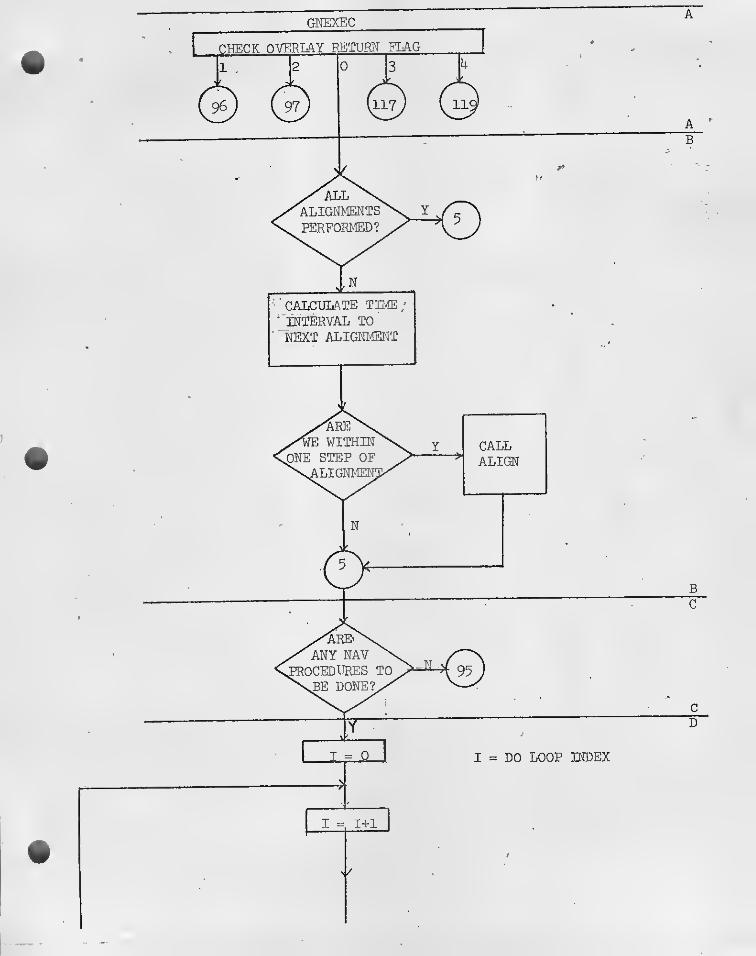
IF (NOVER.GT.O) GO T 0 ( 96 ^ 97 . 117rlT9~)-~'N0VER^~
CHECir~IF~TIMEn‘'0'TERFORM“AN“ArrGTTMENT ^if(lign.ge.nalign) go to 5
KLIGN=LIGN+1aTLIGN=AeS (Y (1) - TALIGN(KLIGN)
)
IFtOTLIGN.G^'P (1))- GO- TO' 5^
CALL ALIGN/CONTINUE— -
^
CHECK IF ANY N A V IG AT ION /ROC EDURES CALLED FOR ON THIS F
IF (NPFR.EQ.O) • GO TO ~93
"
~~~7rC_
CYCLE THROUGH LIST OF DEFINED PROCEDURES B
DO 90 I = 1-,NPER-CHECK IF PROCEDURE APPLICABLE TO THIS PREMANEUVER PERIC
I F ( N Fn )V N EV NGU T DET^ 0 "TC" 9"
THIS SENSOR IS OFF EIF(NM(I) .EQ.Q) GO TO2 0
--~~
~EOEFInF tiME SINCE'LAST TIG FIF (NGUIDE.EQ.l) TGL=Y{1)
GNEXEC
GNEXEC'GNEXECGNEXEC"GNEXECGNEXEC
GNEXECGNEXECGNEXECGNEXECGNEXEC
GNEXECGNEXECGNEXECGNEXECGNEXEC
GNEXEC
GNEXECGNEXEC
GNEXECGNEXEC
CHECK IF THIS PROCEDURE IS TO BE 'TERMIMATEOIF(TGN.GT.DTN(I) ) GO TO 20
SET >1 AN EU VER" C 0 M PUT A T I ON^FCA'C A NO RE sFT” W TN ITIF (TCCMP.NE,2) ICOMP=lTLM(T) = 0.'
' " —- —GO TO 90CONTINUECHECK IF W IS TO BE REINITIALIZEDIF (NW (I )‘;iTE70T“G’O~TO“~S5ZERO NARK COUNTERSNS{1) = D
N3(2)=aNS (3) =0SET W REINITIALIZED FLAG
^ NwnDEFINE TIME TAG ON W
TW =Y(11— ^
TLM(I)=D,
1
I
ALIZATIJ
N FLAG GNEXEC 88GNEXEC 89GNEXEC goGNEXEC 91GNEXEC 92GNEXEC 93GNEXEC 9AGNEXEC 95GNEXEC 96Unexec 97GNEXEC 98GNEXEC 99
u^eo cA/<y
ZERO THE W-MATRIX'DO 25'a = lVl8STORE STATE FOR ADVWX(J}=Y(37+J)DO 25 K=l,27
CTN E-X EC
—
—roBGNEXEC 107bNtXtC 108GNEXEC 109GNEXEC 110GNEXEC 111
SUBROUTINE GNEXEC
WE(J,K)=0. .
-XOAITTH E DIAGONATT"DO 30 J=l,3WE ( J vJ) -uspmWE ( J4-3, J<-3)=USV ( I)
WE( J+6f J+6)=UTP(I)
COC 6600 FTN V3.0-P30|8 OPT=l 08/29/72 11,32.27,
GNEXEC 112
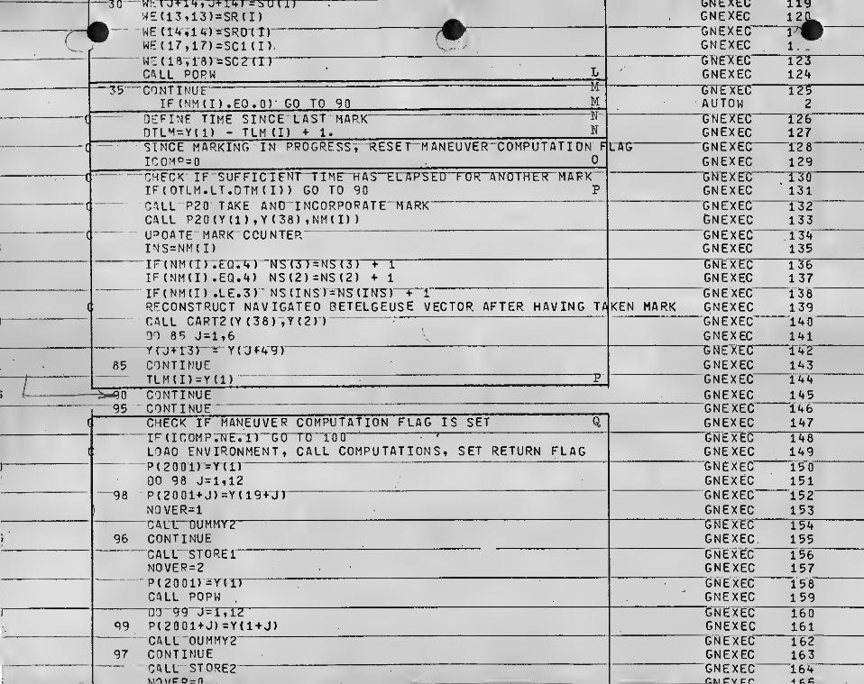
——30 • wh-n3^i4» J+14J = :
^ WE(13,13)=SR(I) ^bNtXtU 119GNEXEC 12^HM WE ( 14-^1 4-) =-SR0T T) ~7^T WE(17,17)=SCi(I), -v.
GNEXECGNEXEC
.1. .
- -- Wc(18vr8)-=SC^fT^—
CML POPW I»
GNtXEC 123GNEXEC 124—35 ‘CONTINUE
IF (NM (I) .EQ .0)' GO TO 90 MGNEXEC 125AUTOW 2
( define TIME SINCE'LAST MflRK“" ' '' ” ^
nTLM = Y{ 1) - TLM (I) +1. NGNEXEC 126GNEXEC 127
C SINCE MARKING IN PROGRESSV reset-maneuver COMPUTATION F
ICOMP=0 0L-Tn; GNEXEC ^1"28
GNEXEC 129—(— CHECK IF SUFFIClENT‘TIMr-KA3 'EL'A'PSED''FOR"AlTaTR'ER“MAPX“‘
IF( OTLM.lt. OTM ( I) ) GO TO 90 PGNE X EC proGNEXEC ' 131
CALL P20 TAKE AND ‘INCORPORATH"HARKCALL P20 (Y (1) tY (33) ,NM(I) )
GNEXEC 132GNEXEC 133
"C UPDATE MARK COUNTER"INS=NM(I)
GNEXEC 134GNEXEC 135
IF (NM fl ) ".EQT^") NET5T^TTST7T“n^TIF (NM(I) .EQ.4) NS(2)=NS(2) + 1
GNEXEC 136GNEXEC 137
(
IF(NM(I) .LE.3)‘ NS(INS)=NS(rN5) + IRECONSTRUCT NAVIGATED BETELGEUSE VECTOR AFTER HAVING TA
GNEXEC 138KEN MARK GNEXEC 139
CALL CART2(Y (38) ,Y(2) )“
DO 85 J=l,6GNEXEC 140GNEXEC 141
Yrjtr3i~"^" Y( JFV9)85 CONTINUE
GNEXEC r42GNEXEC 143
/• TLM(I)=Y(1) P GNEXEC 144CONTINUE GNEXEC 1U5
(
“ 95 CONTINUE— GNEXEC 146GNEXEC 147CHECK IF MANEUVER COMPUTATION FLAG IS SET Q
(
I’^dCOHP.-RET'lT GO TO rOTT”'
LOAD ENVIRONMENT, CALL COMPUTATIONS, SET RETURN FLAGCHEiEC 146GNEXEC 149
I 'P( 200‘1)=Y(I}DO 98 J=l,12
GNEXEC 150GNEXEC 151
'""98 P(2a01 +J)=Y(19 + Jl1 NOVER=l
GNEXEC ^152
GNEXEC 153
»
CALL UUMMYi:96 CONTINUE
GTIEXEC 154GNEXEC 155
- CALL'STORElNOVEP=2
GNEXEC 156GNEXEC 157
'
P(20 01)=Y'(I'J^
^
1
CALL POPW.
GNEXEC 158GNEXEC 159
1 DO 9g“J=l,i2^
99 P(2001+J)=Y(1+J)GNEXEC 160GNEXEC 161
CALL"DUMMY297 CONTINUE
GNEXEC 162GNEXEC 163
CALL STOREEKl'YWFO-fL .
GNt XtC 164CJdCYcr ^c.c
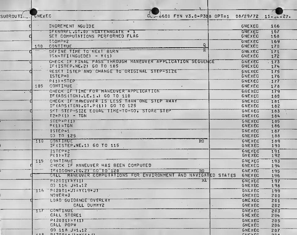
NEXEC -l&OQ FTN V3.0-P3 o| 8 0PT=1 08/29/72 .ll.J^27
increment NGUIOE GNEXEC
SET COMPUTATIONS PERFORMED FLAGT C0 M P=
2^
CONTINUEDEFINE TIME' TO~MEXT" BURNTCN=TFI (NGUIOE) - Y(l)CHECT<-l‘riT:NAi:“P'/rS-S~rHROUGH MANEUVER APPLICATIO^IF(ISTEP.NE.2) GO TO 105RESET ISTEP AND"'CHANGE'“TO~ORTGTNAl STEP-STZEISTEP=QP( 1) -STEP'CONTINUECHECK"! FTTME FOR"M’aNEUVER APPlICAriCNIP (ABS (TGN).LE. 1 .) GO TO 110CHECK" IF^M PNEUVETT-IS EES^TFrAN ONE S I EP AWAYIP(ABS(TGN).GT,P(1) ) GO TO 125S‘-:T STEP-SIZE-EQUAL-TTME-TO-GO, STORE' STEPT2=P (1) - TGNSTE^-=prnP(l) =TGNISTEP = 1
GO TO 125 •
CONTINUEIF (ISTEP. NE.l) GO TO 115TSTEP^Z
'
P(1)=T2CONTINUE ^
^
CHECK IF MANEUVER HAS BEEN COMPUTEDI '^
{ I C 0M P‘.‘EQ ;'2')~~GO~T 0~r2 0
CAUL FUTNEUVER COMPUTATIONS FOR ENVIRONMENT ANDP ( EH aTT^T(nDO 116 J=l,12P ( 20 an-UT =Yri9>T)N0VER=3LOAD-GUTDANCE’TTVTRrAT
CALL OUMMY2CANTimJE
^
CALL STORElP(200ir=Y(nCALL POPWDO lia J=l,12
NAVIGATIEO STATES
GNEXECGNEXECGNEXECGNEXECGNEXECNEXEC
GNEXECGNEXECGNEXECGNEXECGNEXECGNEXECGNEXECGNEXEC"GNEX£C_"GNEXEC"GNEXECGNEXECGNEXECGNEXECGNEXEC“GNOECGNEXECNEXEC
GNEXEC'GNEXECGNEXECGNEXECr M c V cn o n Q

UOMEW-t*LOAD GUIDANCE OVERLAY
CONTINUE“ CAtr-STCTRE2NOVER=a -—INCREMENT NGUIOE
‘
lECNRRFLTGTVO) NGZCONTINUEPERFORM MANEUVER
—
NGUIOF=NGUIDE+l
GNEXECGNEXEC"GNEXeGNEXECGNEXECGNEXECGNEXEC_GNEXECGNEXECGNEXECGNEXECGNEXEC
UBROUTINE GNEXEC
NV=NGUIDE - 1
CACL" DELTAV{CALL STORESICOMP=0"T.TNTrNUERETURN —
"
ENO
COC 6600 FTN V3.0-P308 OPT=l 08/2.9/72 11.32*27
GNEXEC 221
P GNEXEC 223Ri GNEXEC 22if
GNEXEC 225G N EX EC 2 26
GNEXEC 227


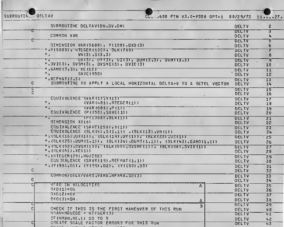
ROUTINE DELTAVROUTINE APPLIES MANEUVER BASED OR ESTIMATED STATE COM-
PUTATION TO ESTIMATED s/c STATE. ALSO COMPUTES EEEECTOF ACCELEROMETER SCALE FACTOR ERROR, PLATFORM MISALIGN-MENT AND CUTOFF UNCERTAINTY. ON APPLICATION TO ACTUALSTATE, VECTORS AND MATRICES INVOLVED IN THESE CALCULA-
TIONS ARE:
DXD NOMINAL DELTAV IN LOCAL VERTICAL IRAME, THISDELTAV IS COMPUTED FROM ESTIMATED STATE AND
IS THE ONBOARD ESTIMATE OF THE APPLIED BURN.
VECTOR OF ACCELEROMETER SCALE FACTOR ERRORS,
S SCALE FACTOR DISTURBANCE MATRIX, I- oW'
VN VECTOR OF CUTOFF UNCERTAINTY ERROR.
UNIT VECTORS OF THE ESTIMATED LOCAL VERTICALFEIAME.
DUM^ TRANSFORMATION FROM BRF TO ESTIMATED LOCALVERTICAL FRAME.
DUMT^ TRANSFORMATION FROM ESTIMATED LOCAL VERTICALFRAME TO BRF. (= DUM^)
REIMAT TRANSFORMATION FROM BRF TO ESTIMATED PLATFORMAXES.
DVI NOMINAL DELTAV IN BRF.
DVSM DELTAV IN ESTIMATED PLATFORM FRAME WITH SCALEFACTOR ERRORS APPLIED.
DVSME DVSM + VN
GAMD MATRIX OF PLATFORM DRIIT ERROR ANGLES
.
DUI^ S X REFMAT *
DUM^ GAMD X REFMAT
DUMT^T T
REFMAT X GAMD
DVIE DELTAV IN BRF DISTURBED BY SCALE FACTOR ERROR,CUT-OFF UNCERTAINTY AND PLATFORM MISALIGNMENT,
DVIE=REFMAT^ x GAMD^ x [S x REFMAT x DUMT
22X DXD + VN]
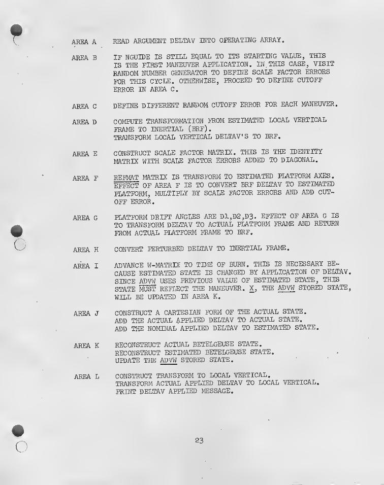
AREA A READ ARGUMENT DELTAV INTO OPERATING ARRAY.
AREA B IF NGUIDE IS STILL EQUAL TO ITS STARTING VALUE, THIS
IS THE FIRST MANEUVER APPLICATION. IN. THIS CASE, VISIT
RANDOM NUMBER GENERATOR TO DEFINE SCALE FACTOR ERRORS
FOR THIS CYCLE. OTHERWISE, PROCEED TO DEFINE CUTOFF
ERROR IN AREA C.
AREA C DEFINE DIFFERENT RANDOM CUTOFF ERROR FOR EACH MAIJEUVER.
AREA D COMPUTE TRANSFORMATION FROM ESTIMATED LOCAL VERTICAL
FRAME TO INERTIAL (BRF).
TRANSFORM LOCAL VERTICAL DELTAV S TO BRF.
AREA E CONSTRUCT SCALE FACTOR MATRIX. THIS IS THE IDENTITY
MATRIX WITH SCALE FACTOR ERRORS ADDED TO DIAGONAL,
AREA F REFMAT MATRIX IS TRANSFORM TO ESTIMATED PLATFORM AXES.
EFITI'cT OF AREA F IS TO CONVERT BRF DELTAV TO ESTIMATED
PLATFORM, MULTIPLY BY SCALE FACTOR ERRORS AND ADD CUT-
OFF ERROR.
AREA G PLATFORM DRIFT ANGLES ARE D1,D2,D3. EFFECT OF AREA G IS
TO TRANSFORM DELTAV TO ACTUAL PLATFORM FRAME AND RETURN
FROM ACTUAL PLATFORM FRAME TO ERF.
AREA H CONVERT PERTURBED DELTAV TO INERTIAL FRAME.
AREA I ADVANCE W-MATRIX TO TIME OF BURN. THIS IS NECESSARY BE-
CAUSE ESTIMATED STATE IS CHAls'GED BY APPLICATION OF DELTAV.
SINCE ADVW USES PREVIOUS VALUE OF ESTIMATED STATE, THIS
STATE MUST REFLECT THE MANEUVER. X, THE ADVW STORED STATE,
WILL BE UPDATED IN AREA K.
AREA J CONSTRUCT A CARTESIAN FORM OF THE ACTUAL STATE.
ADD THE ACTUAL 4i.PPLIED DELTAV TO ACTUAL STATE.
ADD THE NOMINAL APPLIED DELTAV TO ESTIMATED STATE.
AREA K RECONSTRUCT ACTUAL BETELGEUSE STATE.
RECONSTRUCT ESTIMATED BETELGEUSE STATE,
UPDATE THE ADVW STORED STATE.
AREA L CONSTRUCT TRANSFORM TO LOCAL VERTICAL.
TRANSFORM ACTUAL APPLIED DELTAV TO LOCAL VERTICAL.
PRINT DELTAV APPLIED MESSAGE.
O 23
SUEROUTIK, DFLTAV CL>.- o600 FTN V3.0-P308 OPT=l 08/29/72, ll.ow.27
SUBROUTINE OEIT A V (OU ,0V .DW) DELTVDELTVDELTVCOMMON VAR
DIMENSION VAR(5600), Y ( 10 0 ) , 0X0 (3)
. P ( 5 0 0 0)“^-NTEGERri 0 OrT-SLK-frOID, VN(3) ,S(3,3)
DKtT) , UYr3),
DELTV"DELTVDELTVDELTV
^,0VI(3), 0VSM(3), ui\o;, UZ(3), UUM(3,3r,' OUMI (3,3), DVSME(3) , OVIE (3)
^,GAMQ{SV7V^"XE{12)*, SAVE(950)»,REFMATf3-;^)
SUBROUTINE TO APPLY A LOCAL HORIZONTAL DELTA^-V TO A BETEL VECTOR
EOUIVAL-ENDE-TVARTnTYTlTO(VAR (401) ,NTEGER(1)
)
(VAR (60I)",P (171“^EQUIVALENCE (P (350 ) , SAVE( 1)
)
DELTvDELTV 100 EL T V 11
' DELTV 12DELTV 13DELTV 14
DELTv 15DELTV 16DELTV 17DELTV 18DELTV 19DELTV 20
r TPTlTBirrTBUX'TTnDIMENSION X(18)EQUIVALENCrTSAVF(258T,X(l))EQUIVALENCE ( BL K (4 ) , S ( 1 , 1 ) ) , (BLK ( 13 ) , VN (1)
)
, (3LK(16) ,UX(1) ) , (BLK (1 9) ,UYTITT; ' ( BLX(22) , UZ C 1) )
(BLK (25) ,OUM (1, 1) ) , ( BL K ( 34) ,DU MT ( 1 , 1) ) , (BLK (43) ,GAMD(1,1) )
^.•nLfC'(52')TDVS’MTn7~^“CBLXT5T) ,DVSMt(l) ) , (BL K ( 58 ) , DVI E (1) )
(3LK(B1) ,XE(1)
)
V, (MTEGER (29) ,NGUTDEI ^
EQU IVALENCE (SAVE (19) ,REFMAT (1,1))» . (Y(98),ni) , (Y(C9) ,02)7' (YdOOy ,037
DELTV 21DELTV 22DELTV 23DELTV 24DELTV 25DELTV 26DELTV 27DELTV 28DELTV 29DELTV 30DELTV 31DELTV 32
CaMMOTslVDELVT-VAR-^TVTrRXn^r^ so { 37 DELTv ^C DELTV 34c
1
ifg v“eloc1Yif§' ” ^QXD(1)=DU
DELTV 35DELTV 36
DXD(2)‘=D\r
DXD(3)=DW. ADELTV ^ 37DELTV 38
c
c CHECK IF THIS IS THE FIRST MANEUVER OF THIS RUN^ DELTv 39
DELTV 40
3
NMAN=NGUIDE"- NTFGERCS) '
IF (NMAN.NE.l) GO TO 5
DELTV 71DELTV 42
‘ ci i
CREATE SCALE FACTOR ERRORS“FDR“THIS“RUN DELTV 43

^ rZT^LrNORN(U,NF VAkS)Sn(3) =UNURN(0,NFAMfl,l,,VAR$)CONTINUEOEFINF application ERRORVN (1 > =UNURNrO i'NFAMATOViTARTrrVN(2)=U.NURN( 0,NFAMA,0. , VARA)VN"rrr=u nur-r ( o , n f ahatd ; , v arthT^'OM^jT^ btLTAV IN ASSUMED REFERENCE FRAMEC'iLl:“UVEC{Y(38r7Y(39)TY{40)TUT)CALL UCPOSS(UX^ Y (41) ,U2)CALL” UCROSS(UZ,UYVUY) ^
CALL TRN(UX,UY,UZ,OUM,DUMT)
BC
VD
DELTAV
CALL MATMUL(OUMT ,DXD , OV I , 3 , 3 , 1
)
COMPUTE^ACTUAL "DELTAV “A PPL'IED
—
COMPUTE SCALE FACTOR MATRIX '
COC 6600 FTN V3.0-P30 B OPT=l
DO TO 1 = 1,300 10 J=l,3
-1 S(I,J) = 0.
IF(I,EQ.J) S(I,J)=SD(I)^0 --CONTTNUE ^ K
CALL MA IHUL(S,RbhMA ! ,UUH, 3, 3,3) FCALL MATMULCDUM ,DVI ,OVSM,3, 3,1) '
CALL MATA00(0VSM,VN,0VSME,3,1,1 ) FU
'
UMPU I L PLA I hURF HICALILNMET I‘ M
'
ATR"
J7—— a
CALL MAT(D3,D2,01,1,3,2,GAM0)CALL- MA TMUL ( G AMDTT^EFMATVDUTTT^ 3,3)CALL MATRAN(DUM,3,3,DUMT)^ I'M t 1 f
T(LL MA I MULdlLM ! ,'lH;SML , U V 3 L 3
"^ALL ADVW ( Y(l)~, Y (38) )
16
CONSTPUCT CART E S’I A N’ ENV IRONMENT VECTOR'CALL CARTl (XE,Y ( 20)
)
D0-1 5—J = IT3“XE ( J+3) =XE {J+3) + DVIE(J)Y(J^-40)=Y(J4_4iL) » DVKJ)
OELTVOELTVDELTVDELTVDELTYDELTVOELTVOELTVDEi;T\rDELTVDELTVDELTV
08/29/72
OELTV"DTUTYDELTV-DELTVDELTV'DELTVOELTV"DEUTYDELTVDELTVOELTV-DELTVDELTV"DELTYDELTVDELTVDELTV"DELTVDELTV"DETTVDELTV"DELTVOELTV-DELTV
45
"W505152Y3"54
-55-
56
11.32. 27*
57
TF59"60"
61“62'
63'EY65
“66
“
67"68
69TY71-72
73-74-
75TY77
"78
7
n cr • T >1

‘Oa-lZ^-lTTBX(I) = Y(374-I)
' CONTINUE '
C^LL TRN(UX,UY,UZ,DUM,OUMT) '——
_
CiiLL MATMUL(0UM,0VIE,DVlTJ-,-3TrJP?INT 100, (nXD(I),T = l,3)i (DVI (I) ,1 = 1,3)
i
”PaRM-aT(/lXV35HTHF'N*AVlGftTI0N"RURN”“ESTTMATE‘n:s"DU = TF‘id'
lPn.3, 5H DW=,F10.3,/1X,35HTHE ACTUAL COMPONENTS WERE2F n . 3r-5K~ DV= , Fr0 .'3r'5H -bwi' ,Tr 0V3T
RETURN£N|0
OU = ,
OELTVDELTVDELTVOELTV'DELTVDELTV"UErTT/DELTVDELTVDELTV'OELTV
ODCaOoOoCDOO
ro;
O:
vD
Co
-*4
CTi
vn
-f",
W
fV3

S' 76 77 £
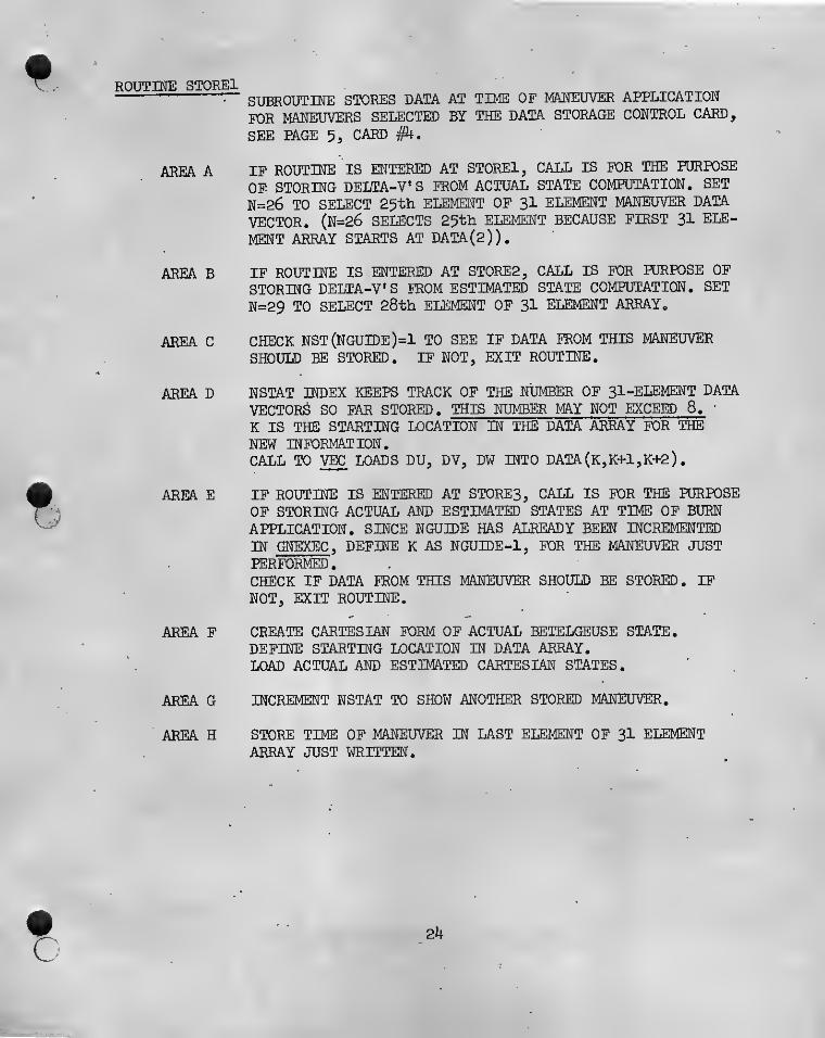
ROUTINE STOREl^ SUBROUTINE STORES DATA AT TIME OF MANEUVER APPLICATION
K)R MANEUVERS SELECTED BY THE DATA STORAGE CONTROL CARD,
SEE PAGE 5, CARD #4.
AREA A IF ROUTINE IS ENTERED AT STOREl, CALL IS FOR THE PURPOSE
OF STORING DELTA-V'S FROM ACTUAL STATE COMPUTATION. SET
N=26 to SELECT 25th ELEMENT OF 31 ELEMENT MANEUVER DATA
VECTOR. (N=26 SELECTS 25th ELEMENT BECAUSE FIRST 31 ELE-
MENT ARRAY STARTS AT DATA (2)).
AREA B IF ROUTINE IS ENTERED AT ST0RE2, CALL IS FOR PURPOSE OFSTORING DELTA-V* S FROM ESTIMATED STATE COMPUTATION. SET
N=29 TO SELECT 28th ELEMENT OF 31 ELEMENT ARRAY.
AREA C CHECK NST(NGUIDE)=1 TO SEE IF DATA FROM THIS MANEUVER
SHOULD HE STORED. IF NOT, EXIT ROUTINE.
AREA D NSTAT INDEX KEEPS TRACK OF THE NUMBER OF 31-ELEMENT DATA
VECTORS SO FAR STORED, THIS NUMBER MAY NOT EXCEED 8. -
K IS THE STARTING LOCATION IN THE DATA ARRAY FOR THENEW INFORMATION.CALL TO V^ LOADS DU, DV, DW INTO DATA(K,K+1,K+2)
.
AREA E IF ROUTINE IS ENTERED AT STORES, CALL IS FOR THE PURPOSEOF STORING ACTUAL AND ESTIMATED STATES AT TIME OF BURNAPPLICATION. SINCE NGUIDE HAS ALREADY BEEN INCREMENTEDIN GNEXEC , DEFINE K AS NGUIDE-1, POE THE MANEUVER JUSTPERFORMED
.
CHECK IF DATA FROM THIS MANEUVER SHOULD BE STORED . IFNOT, EXIT ROUTINE.
AREA F CREATE CARTESIAN FORM OF ACTUAL BETELGEUSE STATE.DEFINE STARTING LOCATION 3N DATA ARRAY.LOAD ACTUAL AND ESTIMATED CARTESIAN STATES.
AREA G INCREMENT NSTAT TO SHOW ANOTHER STORED MANEUVER.
AREA H STORE TIME OF MANEUVER IN LAST ELEMENT OF 31 ELEMENTARRAY JUST WRITTEN,
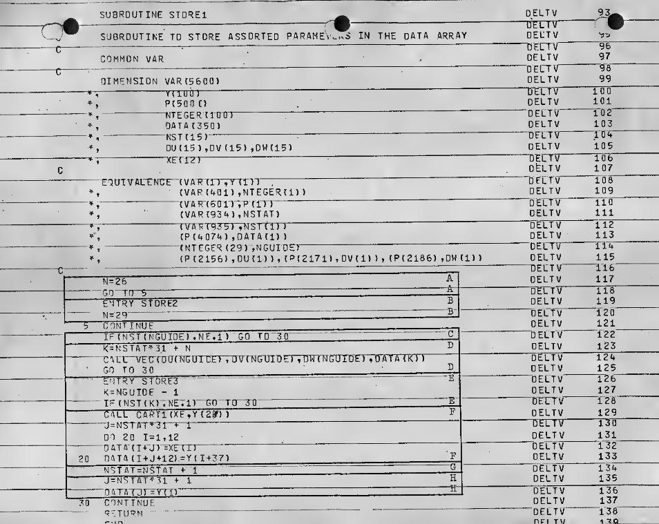
SUBROUTINE TO STORE ASSORTED PARAMEVw.vS IN THE DATA ARRAY OELTV
COMMON VAR OELTVUtL 1 V
DIMENSION VAR(560Q) OELTVoruTV
P(500 C)
NTEGER'trtrtnOATA(350)NS T ( 1 5 r
0U(15) ,0V (15) ,0W(i5)
E0UTVT5LENCE “(VA“R(1) ,Y (1)1(VAP(4G1) ,NTEGER(i)
)
{ VAR'T6'0 n^,P (D")
(VAR(934) ,NSTAT){rA"RTqT51'7N srtiTi(P (4074) , DATA (1)
)
(NTEGER (29) ,NGUITir>(P (2156) ,DU(1) ), (P( 2171) , OV(l) ), (P( 2186) ,OW (1)
)
N-26GO 'TO 5
E'JTRY STORE2 — ---
CONT iNUeIF (NST (NGUIDE) ,NF.l ) GO TO
~3~0~
K=NSTAT^31 + N
ENTRY STORESK=NGUIDE - 1
IF ( NST { K) VNE7IT~GD-TCrTOCALL CAPTl (XE,Y (2^)
)
U = NSTAT^3T“^r-l00 20 1 = 1,120ATA-{T + U) =XETT)DATA (I+J+12)=Y(I+37)
nATATJr = Y~f'
CONTTNUF-RFTUPM
OELTVOELTVOELTVDEl-TVOELTV
UtL I V
OELTV"DEtTV'OELTV"TOTTVOELTV‘OELTVOELTV'OELTVOELTVOELTVOELT^
“DEL“T\rDELTV_OELTVOELTVOELTV 124OELTV 125OELTV 126OELTV 127OELTV 128OELTV 129
OELTV 134OELTV 135OELTV 136OELTV 137OELTV~ 138npj T\/ 1 7QI- • I r\

OV70AT r~'

ROUTINE OUTDATTHIS ROUTINE DUMPS THE DATA(350) ARRAY AT THE END OF
EACH MONTE CARLO CYCLE. THIS PROVIDES A VISUAL INSPEC-
TION OF THE DATA BEING WRITTEN ONTO THE LOCAL MASS
STORAGE FILE.
AREA A WRITE OUT THE CURRENT VALUE OF THE MONTE CARLO RUN INDEX.
AREA B DUMP THE 8 MANEUVER DATA VECTORS.
AREA C SAME AS AREA A.
:)
AREA D DUMP THE 10 PLATFORM ALIGNMENT DATA VECTORS.
AREA E DUMP THE USER SPECIFIED PORTION OF DATA.
c25

UBROUTiO 'TuTOATr
C'-u. 6600 FTN V3.0-P308 OPT=l 08/29/72 11. ^...27.
SUBROUTINE OUTDAT DELTV 140
COMMQN-VAROIMF^NSION VAR(5&00), P(500G), DATA(350)E'3UrVALENCE“(VAR(B(riT;'P'(lT')EQUIVALENCE (P ( 4074) ,DAT A (1)
)
M^UN = nATA( 1)
W?ITE(6,100)
DELTV"OECTVDELTV'DELTVDELTV
DELTVNRUN
CO 5 r= 1,31 - -
5 WRITE(6,105) DATA(I+ 1),DATA(I+ 32),
D
ATA (1+ 63) ,OA TA(I+ 94)DELTVDELTV
Ibl152
5* ,
-" OATA (1^1250 ,T) AT7r(TT'i56TTD ATTTTT+rETTTDTJ
[DELTV 153
W^TE (6,110) NRUK
DQ 10 1=1,7W?ITE(6,115) OAT A (1 + 250 ), DATA (1 + 257) , DATA ( 1 + 264)
Tl'AT7SrrTZ7T)TlTATATr+'2rgyTr!'ATX("r+^g5‘)'0ATA(I+292) , DAT A (1+299) ,OATA (1 + 306)0ATA(I+313)
DELTVDELTVDELTV_“DELTVDELTVDELTVDELTV'DELTVDELTV
VECTOR/MANEUVER DATA FOR RUN NO.,I4,10H FOLLOWS DELTV
FORMAT( 1X,8E15.6) DELTVFORMAT r/50“X,’2 9HALT(rNMEHT~Hr5TO‘RynFOR'”RXm“WD'77r2r,TOtrT‘OILOWS- ,/) DELTVFOPMAT(1X,10E13.4) DELTVFORMAT (74-4X, 47H A SSORTED' OTHER-^fTJRIT'm WN'-TTNXYnnO“lJ'rrR“‘r^ OWS - , DELTV
3(/lX,8El5.6)f/lX,6E15.6) DELTV. TRN DELTV
END DELTV

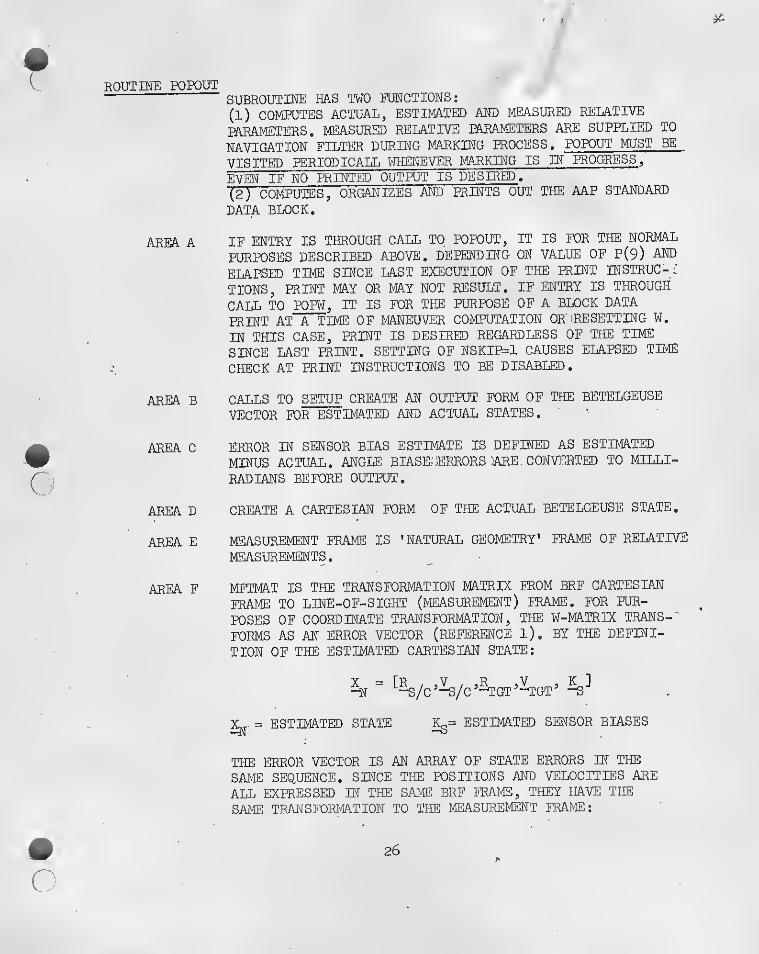
' >
routhte popoutSUBROUTINE HA.S TWO FUNCTIONS;
(1) COMPUTES ACTUAL, ESTIMATED AND MEASURED RELATIVE
PARAMETERS. MEASURED RELATIVE PARAMETERS ARE SUPPLIED TO
NAVIGATION FILTER DURING MARKING PROCESS. POPOUT MUST BE
VISITED PERIOD ICALL WHENEVER MARKING IS IN PROGRESS ,
EVEN IF NO PRINTED OUTPUT IS DESIRED".
(2 ) COMPUTES, ORGANIZES AND PRINTS OUT THE AAP STANDARD
DATA BLOCK.
AREA A IF ENTRY IS THROUGH CALL TO POPOUT, IT IS FOR THE NORMAL
PURPOSES DESCRIBED ABOVE. DEPENDING ON VALUE OF P(9) AND
ELAPSED TIME SINCE LAST EXECUTION OF THE PRINT INSTRUC-l'
TIONS, PRINT MAY OR MAY NOT RESULT, IF ENTRY IS THROUGH
CALL TO POPW, IT IS FOR THE PURPOSE OF A BLOCK DATA
PRINT AT A TIME OF MANEUVER COMPUTATION OR 'RESETTING W.
IN THIS CASE, PRINT IS DESIRED REGARDLESS OF THE TIME
SINCE LAST PRINT. SETTING OF NSKIP=1 CAUSES ELAPSED TIME
CHECK AT PRINT INSTRUCTIONS TO BE DISABLED.
AREA B CALLS TO SETUP CREATE AN OUTPUT FORM OF THE BETELGEUSE
VECTOR FOR ESTIMATED AND ACTUAL STATES,
AREA C ERROR IN SENSOR BIAS ESTIMATE IS DEFINED AS ESTIMATED
MINUS ACTUAL, ANGLE BIASESERRORS )ARE CONVERTED TO MILLI-
RADIANS BEFORE OUTPUT,
AREA D CREATE A CARTESIAN FORM OF THE ACTUAL BETELGEUSE STATE.
AREA E MEASUREMENT FRAME IS 'NATURAL GEOMETRY' FRAME OF RELATIVE
MEASUREMENTS.
AREA F MFTMAT IS THE TRANSFORMATION MATRIX FROM BRF CARTESIAN
FRAME TO LINE-OF-SIGHT (MEASUREMENT) FRAME. FOR PUR-
POSES OF COORDINATE TRANSFORMATION, THE W-MATRIX TRANS-'
FORMS AS AN ERROR VECTOR (REFERENCE l). BY THE DEFINI-
TION OF THE ESTIMATED CARTESIAN STATE:
^ = ESTIMATED STATE Kc,= ESTIMATED SENSOR BIASES
THE ERROR ‘VECTOR IS AN ARRAY OF STATE ERRORS IN THE
SAME SEQUENCE. SINCE THE POSITIONS AND VELOCITIES AREALL EXPRESSED IN THE SAME BRF IRAME, THEY HA'VE THE
SAME TRANSFORMATION TO THE MEASUREMENT FRAME;
26
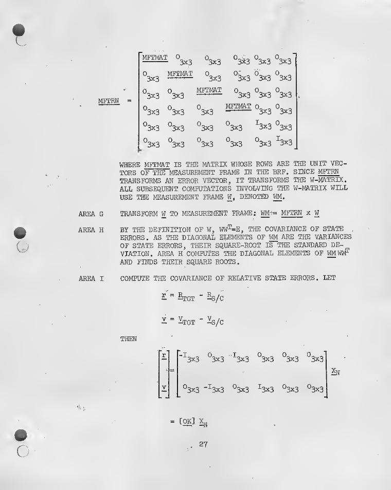
MFTlvlAT 0^ ^3x3
"3x3 on
0°3x3
"3X3
Sx3METMAT % 03x3 "§x3 °3x3
"3X3
^3x3 °3x3METMAT "
3x3 °3x3"3X3
^3x3 "3x3"3x3
METMAT°3x3
"3X3
*^3x3"3x3
"3x3
"3x3 ^3x3 "
3X3
*^3x3"3x3
"3x3
"3x3 °3x3 ^3x3
WHERE MFTMAT IS THE MATRIX WHOSE ROWS ARE THE UNIT VEC-
TORS OF THE MEASUREMENT FRAME IN THE BRF. SINCE MFTRN
TRANSFORMS AN ERROR VECTOR, IT TRANSFORMS THE W-MATRIX,
ALL SUBSEQUENT COMPUTATIONS INVOLVING THE W-MATRIX WILL
USE THE MEASUREMENT FRAME W, DENOTED WM .
AREA G TRANSFORM W TO MEASUREMENT FRAME; WM^= MFTRN x W
AREA H BY THE DEFINITION OF W, WW^=E, THE COVARIANCE OF STATE
ERRORS. AS THE DIAGONAL ELEMENTS OF m ARE THE VARIANCES
OF STATE ERRORS, THEIR SQUARE-ROOT IS THE STANDARD DE-
VIATION. AREA H COMPUTES THE DIAGONAL ELEMENTS OF WMWM"^
AND FINDS THEIR SQUARE ROOTS.
AREA I COMPUTE THE COVARIANCE OF RELATIVE STATE ERRORS. LET
- ^ Stgt " ^/c
- “ -TGT " ^/C
THEN
^3x3 °3x3 '^3x3 °3x3 °3x3 °3x3
°3x3 "^3x3 °3x3 ^3x3 °3x3 °3x3
= [OK] ^
27
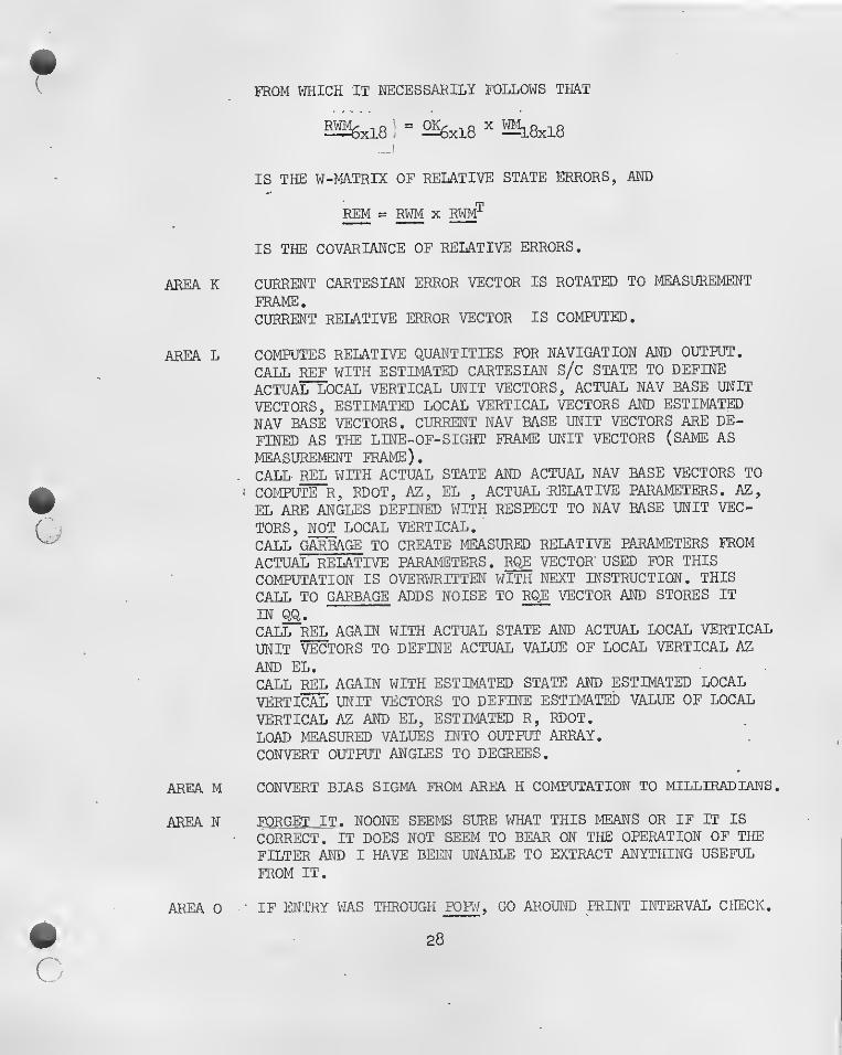
FROM WHICH IT NECESSARILY FOLLOWS THAT
2Sfexl8 ." 256x18 ^ ^8x18
i
IS THE W-MATRIX OF RELATIVE STATE ERRORS, AND
REM = r™ X RWM^
IS THE COVARIANCE OF RELATIVE ERRORS.
AREA K CURRENT CARTESIAN ERROR VECTOR IS ROTATED TO MEASUREMENT
FRAME.CURRENT RELATIVE ERROR VECTOR IS COMPUTED.
AREA L COMPUTES RELATIVE QUANTITIES FOR NAVIGATION AND OUTPUT.
CALL REF WITH ESTIMATED CARTESIAN S/C STATE TO DEFINE
ACTUAL LOCAL VERTICAL UNIT VECTORS, ACTUAL NAV BASE UNIT
VECTORS, ESTIMATED LOCAL VERTICAL VECTORS AND ESTIMATED
NAV BASE VECTORS. CURRENT NAV BASE UNIT VECTORS ARE DE-
FINED AS THE LINE-OF-SIGHT FRAME UNIT VECTORS (SAME AS
MEASUREMENT FRAME).. CALL REL WITH ACTUAL STATE AND ACTUAL NAV BASE VECTORS TO
COMPUTE R, RDOT, AZ, EL ,ACTUAL :RELATIVE PARAMETERS. AZ,
EL ARE ANGLES DEFINED WITH RESPECT TO NAV BASE UNIT VEC-
TORS, M LOCAL VERTICAL.
CALL GARBAGE TO CREATE MEASURED RELATIVE PARAMETERS FROM
ACTUAL RELATIVE PARAMETERS , R^ VECTOR' USED FOR THIS
COMPUTATION IS OVERVmiTTEN WITH NEXT INSTRUCTION. THIS
CALL TO GARBAGE ADDS NOISE TO R^ VECTOR AND STORES IT
IN QQ.CALL^ AGAIN WITH ACTUAL STATE AND ACTUAL LOCAL VERTICAL
UNIT VECTORS TO DEFINE ACTUAL VALUE OF LOCAL VERTICAL AS
AND EL.CALL REL AGAIN WITH ESTIMATED STATE AND ESTIMATED LOCAL
VERTICAL UNIT VECTORS TO DEFINE ESTIMATED VALUE OP LOCAL
VERTICAL AS AND EL, ESTIMATED R, RDOT.
LOAD MEASURED VALUES INTO OUTPUT ARRAY.CONVERT OUTPUT ANGLES TO DEGREES.
AREA M CONVERT BIAS SIGMA FROM AREA H COMPUTATION TO MILLIEADIANS
.
AREA N FORGET IT. NOONE SEEMS SURE WHAT THIS MEANS OR IF IT IS
CORRECT. IT DOES NOT SEEM TO BEAR ON THE OPERATION OF THE
FILTER AND I HAVE BEEN UNABLE TO EXTRACT ANYTHING USEFUL
FROM IT,
AREA 0 IF ENTRY WAS THROUGH POP^f , GO AROUND PRINT INTERVAL CHECK.
28
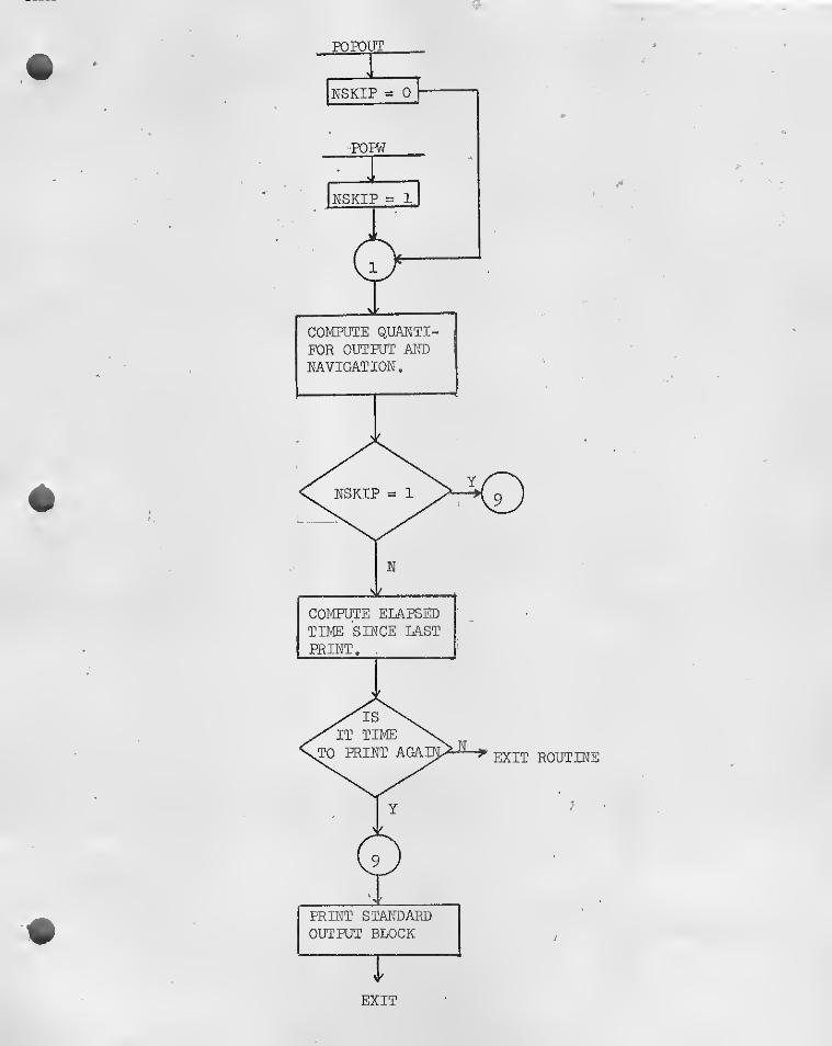
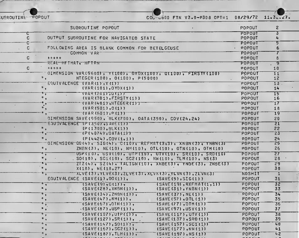
rH—UEROUTINh TOPOUT -m--
C D\j 60 0 FTN V3,0-P308 OPT=l 08/29/72
SUBROUTINE POPOUT
OUTPUT SUBROUTINE FOR NAVIGATED STATE
FOLLOWING AREA IS BLANK COMMON FOR OETELGEUSECOMMON 'VAR ^
+ + + + +
REA tr-Mf-TftA-T—MF-TRN+ + + f +
DIMENSION VA-RtB60Qr , Y ( liron~DYTD(TlU U ) , Q ( 1 0 U) V ' F'IR5^
NTEGERdOO), DdOO), P(5000)EQU I V ALENCE ( V A R (1)-,T (DO
(VAR (101) ,DYOX(l) )
^
(VAR (301) ,FIRSTY (1)
)
(VAR (A01)->NTE(;ER-(tn(VAR (501) ,0(1)
)
(VAR (601) ,P(1) )^
DIMENSION SAVE (950) , 'BLK(700 ) , OATA(350), C0V(24»24)
(P(1300) ,BLK(1))(P( 4074 ) yOATA(I)-)
(P(4424) ,COV(l,l))01 ME-NSI-ON-QO ( 41 Y" S I GT 4 ) Y“C ( 1 0-)T~RE
ZNBN (3 ) , NE (10) , NM (10 ) ,
. SO(IO) , SCl(lO) , SC2(10)7rZ { 4r,~SZT4) V T-ATL-IGNTl'D
X(18) , WE(18,27)XL VE (3 )TYt VE(3)’,ZL-Vr(ZD,
EQUIVALENCE ( S A V F ( 1 ) , 00 ( 1 ) )
,
TS'AV E7 9')TC ( D'r^(SAVE(28) ,XN3N(1) )
,
(SA VE (3 4“)TZNBN ( IT)";
(SAVF(47) ,NM(1) )
,
(SAVF(67) ,nTN (IVT";
(SAVE(87) ,USP(1) ),
(
s
A VrrroTDUT PTxrr;(SAVE(127) ,SR(1) )
,
(
S
A V E ( 1 47)", SOT 1DT;(SAVF(167) ,SC2(1) )
,
{SAVE(187),TLM(1))
OTL(IO) , DTN(IO) , OTMdO)rJi]» u I
, NWdO) , TLM(IO) , NS(3)
XL"? KT‘3I",TX37NT7T",Tn/N (3
)
{SAVE(5) ,SIG(D )
rs'A VE ( 1 9T7REF
M
A Td , iTT(SAVE(31) ,YNeN(l))is A vet 37n NETlT)(SAVE(57) ,OTL (D)(S AVE (77)';XITM (1TT(SAVE(97) ,USV(1))TSWE"(TT/TTUTYnn(SAVE (137 > ,SRD (1))
(SAVE l SCV( IV)
(SAVEd77) ,NW(1))(SAVE (197) , NS { 1)
)
POPOUT
POPOUT
POPOUTpopourPOPOUT"PTDP
POPOUTPOPOUPOPOUT"popoorPOPOUT
“P'ClPtTO
POPOUTTopourPOPOUT"POPOUTPOPOUT
POPOUT"POPOUTPOPOUT
“POPOUTPOPOUTh’UKUU I
POPOUT“POPOUTPOPOUT
POPOUTPOYOUTPOPOUT“P(DPOUrPOPOUTPOPOUTPOPOUTTOPOWPOPOUT_“POPOUTPOPOUTPOPOUT
CO
icp
o
csj
ro
!-i-
If'
’•X)
r«-
co
o'
jo
^c^J
jCNjicMfO;
rororo|t<»fOjroroforoj.
4
-J'.-a-
(SAVE (218) tNALIGN) POPOUT 44(SAVE(229),XNBE(1 ))
9
^SAVE (232) ,YNBE (1) ) POPOUTrSAVE(235TTZNBr£l”)") ,
(SA VE(276) 9 WE {I 9 1) )
””^TvE”r2 58"rrx(i) > POPOUTPOPOUT :•
»
,
(NTEGER(3 0Q ,ICOHP)EQUIVALENCE (SA VE ( 762) , XLVE ( 1) )
POPOUTNOSHIT
482
NOSHIT 3
(SAVE (768) 9ZLVE(1> ) NOSHIT 4(SAVET77n 9 XLYNTITI NOSHIT 5
(SAVE (774) 9 YLVN (1) ) • NOSHIT 6
(SAVE 1777) ,7LVN(in NOSHIT 7
C POPOUT 49
SUBROUTINE POPOUT COG 6600 FTN V3.0-P308 OPT= 1 08/29/72 11*32.27.
EOUIVALENCE (C( 1 ),TW) POPOUT 50
niMENSION OUT(200)
EOUTVALENCEEQUIVALENCE
(BLK (1) ,OUT (1)
)
(NTEGER(-4'2)-jNLINE)
EQUIVALENCE (P(7) ,CGO)•( PCS' TTt: ROT
OIMENSrON- -xNBtiarrXTNC(6) 9
DXSKr'BQT
ocEarrerrXSEC (6)
,
D)rr?T(6T7XTEC ( 6 ) ,
TTRXNTFTDXSC( 6 ), DXTC( 6 ), RXEC(6 )
KTiN ( 4)RQE{4) , Rr)M(4)
EQUIVALENCE (OUT (1) ,XNB (1)
)
(0UT (13)'9 XEBCDT(0UT(25) ,BIASN(1))TOIJTT3TT7BrA SE {‘TTy(OUT (37) ,OBIAS(l)
)
(OUT {43T tXSNC (1))
~
(0UT(49) tXTNCd) )
(OUT (65) ,XSEC(1) )'
POPOUTPOPOUTPOPOUTPOPOUTPOPOUTPOPOUT~po'p'our
POPOUTpopourPOPOUTpopourPOPOUTPOPOUTPOPOUTPOPOUT”POPOUTpopourPOPOUTPOPOUTPOPOUTpoPourPOPOUTPOPour
51525354'55”
565758'59"
60"61"
62
64656667686970_
717273
rniiT r A 1 ^ - YT rn f 9 ^ \ r> I
(ouT(67},oyscr(i))(0UT(73) ,0XTC(1) )
TDUT(7“9T7RyECrDT(OUT (85 ) DXSM( 1) )
outT^^Io!0UT{6I-6'6TOUT (67-72)OUT (77-78)“0UT(7g-84)ouTTffT^gcrra'JT(gi-96)
NflVIGftTEO '(JTrRT'ESl An TGTENVIRONMENT CARTESIAN S/CTNVIRONMENT~CART£'SrA"frTGT "
NAVIGATED MINUS ENVIRONMENT CARTESIAN S/Cl^AVIGATED'l^INOS“ENVTRON"RE7qrnriARTT“Slra(r^^TGT MINUS S/C ENVIRONMENT CARTESIANTTS raA'TEiriTT^ro'^l^\7IR ON M^'ri^ E A S UR E MEN S/C"NAVIGATED MINUS ENVIRONMENT MEASUREMENT TGT
POPOUTPOPOUTp-opourPOPOUT
POPOUTPOPOUTPOPdUfPOPOUTpdPdOTPOPOUTPOPOUTPOPOUT
7576\t7 -
(0UT(91) ,OXTM(l)T POPOUT 79(OUT(g7),DRXM(l)
)
POPOUT 60“TOOTT10'3T ,SIGEM(1TT POPOUT 81(OUT (121) ,REM(1,1) ) POPOUT 82
tUUiVAUtNUt (UUT (157) ,KaN(l) ) POPOUT 83(OUT (161) ,RQE(1) ) . • POPOUT 84
• * , (uUI(lb6),KUM(l)) POPOUT 85c ROO) POPOUT 86u DJI (1-12) N A VIGTJThO ^LTELGEUSE POPOUT
. 87c . OUT(13-24) ENVIRONMENT 3ETELGEUSE POPOUT 88u OUT (2?-“70r“ NAVIGATED “BTASrS POPOUT 89C 3JT(31-36) ENVIRONMENT BIASES POPOUT 90u . OUT (77-42) NAVIGAIED minus ENVIRONMENT BIASES POPOUT 91C nuT(43-48) NAVIGATED CARTESIAN S/C POPOUT 92
93949596979899
100C OUT(97-I07) NAVTGATECrTriNUS~FNVIRONHE'N“riRELATTVE S“T'ATE POPCTUT 101C VECTOR, MEASUREMENT POPOUT 102C OUT(TOT-r7tn ONE-SrGMA-'E'RRORS“~MFASUR’EHETn POPOUT 1 C*3'
C 0UT(121-156) RELATIVE COVARIANCE MATRIX MEASUREMENT POPOUT 104
UBROUTINE POPOUT COC 6600 FTN V3*0-P308 0PT=1 08/29/72 11.32,27,
C 0'JT(157-160). RELATIVE QUANTITIES NAVIGATED
'
POPOUT 105C OUT (161-164) kEla 1 i vt DUANiillES"'tNViRONMENI ^maasitvtmc 0UT(165-168) RELATIVE QUANTITIES OBSERVED POPOUT 107
0
DIMENSION XM(3), YM(3), ZM(3), MFTMAT(3f3>, nUM(3,3) POPOUT 109^ ’ MFTRN (18,18), WM ( 1 8 , 27 ) V 0 K ( 6 , 18 ) , RWM(6-,27r POPOUT 110
'

=-oi
NSKIP'-“0GO TO i
enjtry-p-opNSKIP = 1
CONTt-MUf-
SET-UP THE-NAVrGATEt)-STATE-VECT(mTq-TH£ BH.TELGEUSE fRmtCM I S£TUP(Y(2) ,XNB(1))
SET-UP THE ENVIRONMENT -STATE--VECTOR-TTr^KE^ETErGEUSE~rRffKE—CALL SETUP(Y(20) ,XEB(1) )
B
CREATE THE-NAVIGATEO‘ANa~ENVIRONHEN I BIAS A'RRTiYS~7INirTHrTR“D ]
TO 5 1 = 1,6 C
OIASNCI) = Y(Ifl3)^
BTASEd) = Y(I+31)DT I
A
$ ( I
)
=' 8 1 AS N (
I
r - “B I ASrCT)IP (I .EQ.3.0R.I .EG.4) DBIASd) = OBIAS < I) 0 0 0 . 0
C
5~ CONTINUEC CREATE THE NAVIGATED STATE VECTOR IN THE CARTESIAN FRAME
00 10 -I=TV6XSNC(I) = Y(I+37)— -
- XTNC(I) Y(If43) ^
10 CONTINUE
ECREATE THE“ TRANSTOPMATTON^MATRIOrTfHICH RUlAIbS A VtUlUK HKOM*
CARTESIAN TO THE MEASUREMENT FRAME
YH = UNIT(RANGE)Z’1 =-“UNTT TRS^ “R ANtlETXM = UNIKYM X ZM)
POPOUT“POPOUrPOPOUT-popourPOPOUT
3 FFERE'TIUE—POP OTIT
POPOUT124125
"POPOUT 126POPOUT 127POPOUT 128POPOUTb n b h i 1 T
129
-RttTATE ENVIRONMENT"'CALL nAPTl(0UT(55) .Y(Zn) )
;L
""C CALCULATE THE ERROR VECTOR BET WEEN THE “NAVIGATE 0 AND'ENVIRONl
C VECTORS IN THE CARTESIAN FRAME00 IE 1 = 1,6OXSC(I) = XSNC(I) - XSEC(I)0XTc"rrr^“XTN c ( i
)
"
"”x i E'C'rrr"“
15 continue-C-'I N“T HE CARTESIAN "FR A'ME“C AUCUL'A Tb THE RELATIVE STATE VECTDR”BC ENVIRONMENT STATES OF THE S/C AND TGT
DO 2 0 1=17 6 —RXEC(I) = XTECd) - XSEG(I)
ESVXS* rISiSiinSaSiEBHl iSiamiailHSnnSifiuaissfii^HarMi
POPOUT^POPOUTPOPOUTpoPourPOPOUTismulllli
POPOUTpopourPOPOUTT>OPOUT’POPOUTpoPOuTPOPOUTTopourPOPOUTpopourPOPOUTPOPOUTPOPOUT“PO'POuT_POPOUTPOPOUTP^^UTpopdPOPOPOPOPOPOPOPO

oo
0PT=1 08/29/72 11. 3*.. 27.
POPOUTtill?
CaLLTRM.X M 1 Y M • 7 ^ t M F T M A T , D U M
)
CFEATE THE MATRIX MFTRN WHICH ROTATES THE W MATRIX FROM THETO THE MFASUREMENT”FRAHE
ZERO THE~rnCATTONS""FOR-THE"MAI RIX MFTRN30 25 1=1,18no 25 J=l,18MFTRNdtJ) = 0.0
25 CONTINUE -
SET UP MFTRN AS AN (18 X 18) MATRIX COMPOSED OF 4 (3 X 3) MF2-( 3 -X-3^~I0ENTdTY—M-rTR-rC£-S--AlrTmt3-TtTE~(3TO?T3T^
00 30 1=3,12,3j _ ^
no 30 J=l,3GO 30K=1,3M'^TRN( ( J + L) , (K +D) = MFTMAT{J,K)
“3-0“ CONTTTJUEDO 35 1=13,18— MFTRN ( I , I ) -=-r;*o
35 CONTTNUrROTATE the W MATRIX“IKT0'TME'~MEA‘5URE‘MENT FRATfE G
CALL MATMUL(MFTRN,HF,WM, 18, 18,27) GC A L 0 1J L A TE"T Hr ‘ 0 NE - S I CMA "POSI T 1 0 N—A^Na“V ELTCTTr"irRR'DRS““D'F“THE~MATRIX E IN the MEASUREMENT FRAME H— on - i* 0 1 = 1 V 18
SO = 0.000 - 4 0 0 = 1 f27EO = ED + WM (I, J)»»2
3) MFTjMATS AND
CONTINUE
create the ok MATRIX TO BE USED IN CALCULATING THE RELATIVETN’ THE* me asurement-fr^ahe
00 45 1 = 1,6.
-n-j- 5 Tr^=“iTisOK(I,J) = 0,0
"50 CONTINUE0K(I,T) = 1,0OK(T, (1+6)) = -l.OmM T T Ml I r

u
-J
POPOUTPOPOUT
2032Q(^^RFATE THE RELATIVE W MATRIX IN THE MEASU^MENT FRAME J
cjH IjALl ma I mu
L
t Ul^ , W M , RWM , b , 1 ti , /'
J
UREATE THE RELATIVE COVARIANCE MATRIX IN ,.,e MEASUREMENT FRAh E
POPOUTPOPOUT 2 0 o
jALL MA!kANlKWM,btif/’,RWHI )
CALL MAT-MUKRWM , RW MT , RE M , 6 , 2 7 , 6 ) JPOPOUTPOPOUT
2'D7
208crRFPTA Cr'THE -V ARIANCrS~AL ONTT^rHEDI AGUNA L Oh THE RELATIW“CQI/Triance POPOUT 209c MATRIX WITH THEIR ONE-SIGMAS POPOUT 210
DO 55 1=1,6 POPOUT 211REM(I,I) = SQRT (ABS (REM(I,I) ) ), POPOUT 212
55 CONTINUE poPour 213c CALCULATE THE CORRELATION COEFFICIENTS AND PLACE THEM IN THE LOWER POPOUT 214
SUPROUTINE POP'OUT GDC 6600 FTN V3.0-P3G8 OPT=l 08/29/72 11.32,27.
C TRIANGLE OF THE SYMMETRIC COVARIANCEa .T 6 0 r=l,b
MATRIX POPOUTDODriflT
2159-1 c.
*59
f>-0-
rF(RPM(I,I).EQ,0.0) GO TO 60DO -59 J = l,6 — ^IF{J.GE.I) GO TO 59
J) =-R£M(-^JVl) / t-REM(Ivir»^^M ( J, J) )
CONTINUECONTTNUE ^
^
KROTATRAJ
IN T
RELA
61
T E T H E - ER R0R^V E01 OR-R ET W EEt)-! HE“ N A V IG ATEEr-A'TIO^'NVIRONVEnH '
f^CTORIES FROM THE CARTESIAN TO THE MEASUREMENT FRAMECALL- MATMUL(MFTR^?,OUT (67)-fOUr( SGrrlS-iTSTl)
He MEASUREMENT FRAME, CALCULATE THE DIFFERENCE BETWEEN THET I VE—S-T ATE*"VE CTO-RS'-OF TH E NAVTgA T E D ANO 'E NV IR ONKEN T I RAjADO 61 1 = 1,6DRXM ( I) - OX TM nr----OXSM( t)
^
CONTINUE K
OFFIFLFV
ME THE CURRENT NAVIGATION BASE ATTITUDE FOR THE AZIMUTHATTON ANGLE COMPUTATIONCALL PEF(0UT(43))
COMPUTE THE ENVIRONMENT RELATIVE QUANTITIESrail PFLiiniiT r L_^nF . vMnr . vmoc . 7 wrf ^
AND
POPOUTpopourPOPOUTTopourPOPOUTPOP'OUTPOPOUTpopourPOPOUTpopourPOPOUT
c
tr
POPOUTPOPOUT’POPOUTPOPOUTPOPOUTPOTOUTPOPOUTPOPOUTPOPOUTPOPOUT
217218"
219220'
221'27Z223'224~
225226227
229'2 30'
2312 32’
233‘2’34
235236237238
r>r\ I
CTl A DD N C T SE “TOt NVTH0NWENT ~XJES ET?VTH LECALL GAP6AGE(RQE)
' ® CALX PEL' (OUT [551TRQrr5fUVETYCVE7Znr^COMPUTE THE NAVIGATED RELATIVE QUANTITIES -
CALL' PEL (OUT ( t.3)VRQN,XLVNVYLVNVZLVNrr“PADEG = 57-,29577<55
OPOUTPOPOUTTI'OSHTTPOPOUT"NOSHirPOPOUT
AOO RIASES TO NAVIGATED' RELATIVE QUANTITIESRONd) RQNdT'X' BrASN tr)
SET UR THE MEASURED PEIATIVE QUANTITIES FOR OUTPUTROM(ir = QOd)
CONVERT AXIMUTH AND ELEVATION ANGLES TO DEGREESI R ( T ,“lTT3’)“G‘0~rO”^5ROMd) = RQMd) »RAOFGRTNdT-^-'-RONddPADEG^"ROE( I) = ROEd) ^RADEG
65 CONT INUE'lilUiaUMBUUI niSKSlIHISl^RMISlUim^ EilSfimr' NGLESFTTLX^RA GIANS
STGEM(15) = SIGEM(i5)^iaOO‘
S r GE M ( i 6 r"=~S I G E M ( iX T^l OTJ 0
¥"¥ ¥ ¥ ¥ ¥ ¥ ¥"¥ Ar¥'¥Tf>'¥Tr¥ni.‘¥^¥TT^’¥'¥'¥r¥ ¥
mnxuLATr
POPOUTPOPOUT
251252
POPOUTPOPOUT •
253254
POPOUTJS POPOUT
255256
POPOUT 257POPOUT 258POPOUT 259POPOUT 260
4 »¥¥¥¥ POPOUT 261POPOUT 262
OFTHE EARTH POPOUT 264G'l = CGO^'CRO'^‘^2 POPOUT 2 65
ADVANCE ESTIMATED TARGET TO ENVIRONMENT TARGET POPOUT 266CALL^ OPENl (XTNCVXTEXTSTT) POPOUT 2b/CALL OPEN2 (XTNC , GM, -STT ,RTT , ROT T , VHTT
)
POPOUT 268
EROUTINE POPOUT CDC 6600 FTN V3,0-P30£ OPT=i 08/29/72 11. 32,27
rnVANCE ESTIMATED SPACFCRAFl 10 E'N VI RONHE'NTCALL OPENl (XSNC ,XTEC ,STS)CALL‘"OPEN2 (XSNC VGMV-STS',RTSTRDTSTVHrST
ADVANCE ^^NVIPONMENT SPACECRAFT TO ENVIRONMENT TARGE'I
POPOUTPOPOUTPOPOUT'POPOUTPOPOUTPOPOUT
f\r\ c Ki 4 /vc'r*/'

CHECK IF SUFFICTENr-TIMr-HaSTLP=Y(1) - P(10>
POPOUTpopourPOPOUT
1
'CALL UPbN2 lXStU,UH,-blbA,KISA,RU!SA,VHTSA)^MPUTF CURVILINEAR ERRORS ^
POPOUT 276POPOUT 277^
RTE = RSSCXTECT DTXTECTETVXTETrCTT)^ RDTF = DOT(XTECll), XTEC( 4 ) )/PTEPOPOUT 2
POPOUT 2 / ,VTE - RSS(XTEC( 4 ) ,XT£CT5r,XTErCr6T)VHTE = SGRTtVTE ^''2 - R0 fE^* 2 )
PO PO UT 280POPOUT 281
SE = (ST 3 A - STS + STT)*RTEPOPOUT ?E2POPOUT 283
RE - t-RTE - RTSAf - TRTT^^^^TS)VHE = (VHTE - VHTSA) - (VHTT - VHTS)
POPOUT 284POPOUT 285
RDE = (ROTE - ROTSA) (ROTT -~RDT57PHIO = VHTE/RTE
POPOUT 286POPOUT 287
DVDH~=“ 1 . EYPHTD'^FE“ '
VCF = VHE + OVD H NPOPOUT 288POPOUT 289
TF(NSKIP.E 0.1 ) GCTO-q 'X) POPOUT 290
291'292
293IF ( TU^TCTTP r9 ) )~G'0
~TU" 2UU ^
P( 10 )=YU),
9 CONTINUEC CHECK" FORn’IHr'XO-p'AGEHEat] = '
IF(NLTNE.LT.58) go TO 11oRlNT-g-5NLINE=0
IT CONTINUE ^
C -
c
C ^—PRTT3 r"0UT' THE GOODIESc
POPOUTPOPOUTPOPOUTPOPOUTpoPourPOPOUTPO“POTrT
POPOUTPOPOUTPOPOUTPOPOUTPOPOUTPOPOUTPOPOUT
294295296
'
2972982^99
3F0
30130 2
3 03304305306307
TF fTJLTnE;EQT79r> P^i N T 9 0
C OUTPUT THE NAVIGATED AND ENVIRONMENT BETELGEUSE STATESpi:^IMT-j^n|7;-Y(l-)
^RINT 105PRI>II ii'D-i 'Tmun) ,I=TV12-), (KEO(T) , 1 = 1 , 12 )
C OUTPUT THE NAVIGATED AND ENVIRONMENT CARTESIAN STATESPRINr-I157^(n— '
PRINT 120PR INT"125‘,*TXSNCTTrTI‘nTB'l“r^T(T'NCr(Trrr=r7ET
(XSEC (I ) ,1 = 1 , 6 ) , (XTECCI) ,1 = 1 , 6 )
C uui^UT C ARTESIAN SIAIt ERRORS IN THE MEASUREMENT FRAMEPRINT 130
I NT 135°?INT 140 , (DXSM (I) ,1 = 1 , 6 ) , ( DX TM ( I
)
,
1
= 1 , 6 )
C" nUTPUT PELATIVE STATE ERRORS,' RELATIVE ‘PARAMETERS','”M ARKST'CO VARTATrUEC DF Pn 'V T T \/ r FPPnPF TM TWC MCACllorMCMT PPAMC . AMH TMCOTTAI c>TAiL«nAnr»
POPOUT 308POPOUT 309POPOUT 310POPOUT 311POPOUT 312POPOUT 313POPOUT 314POPOUT 315POPOUT —316POPOUT 317POPOUT 318POPOUT 319POPOUT 320POPOUT 321POPOUT 322
•9 ^ ^9

UEROUTINl popout ,600 FTN V 3 .O-P3 O 8 OPT=l 08/29/72 11.^
C DEVIATIONS
PRINT 150, (DBIASd) ,1 = 1,6) , (ORXM ( I ) ,1=1, 6)
POPOUTPOPOUTPOPOUT
P R I T“1 5 5
PRINT 160, SE, VHE, VCE, RE, ROEPR I NT -1 65 r- ICOMP-,-'- Z T Z-(l’) ^
{RON (I) ,1 =1,4) , NSd), ZTZ(2)
(RQM(T) ,1 = 1,4) , NS(3), ZTZ(4), (REM { 2, 1 > , 1=1 , 6)—( Trrrri -iT6r
SZ(l), (REM(4,I) ,1=1,6)-i S I GE M ( I )Tl^lT6r, S-Ztei-i—( REM (571 ) Tr= 1 76)’
(SIGEM(I) ,1=7,12) , SZ(3) , (REM (6,1) ,1=1,6)
NLINE = NLINE + 29
FORMAT STATEMENTS
V-BAR W-BA
90 FORMAT(//)-'95 FORMAT (l-Hll
^
100 FnRMAT(53X,17HBETELGEUSE STATE ,F8.1)“155 F0RMAT'(T2X 7ri7H'R‘A0"'V£tr CONGITUOE LATIlUUb flLi km 1 1 HUK VtL HtA
’^niNG X-BAR Y-3AR Z-BAR U-8AR V-BAR W-BAV
110 FORMAT (IX, 10 HNAV ,F9. 0 ,2F9.3 , F9 . 2, FI 0 • 2, F9 . 3, 3F11 . 0 , 3F1 0 .2^,
^ nx,'l0RA‘C1 ,T9T072F9;3 , F9. 2,prCrr27F‘9TTr3 FT! . 0 , 3 FI 0 • 2)'
115 FORMAT(/53X,17HCARTESIAN STATE ,F8*1)-120 Fr)RMATT7‘X-,123HXSlBRrr YSTBRF7 ZSTERFO X’SOTB'PF) TS'O (BRF)
^ ZSO(BRF) XT(BRF) YT(BRF) ZT(ERF) XTD(BRF) YTOCBRF) ZT^ 0( P RFT) ^
POPOUTpopour-POPOUTTOPPOPOUT-popour"POPOUTTOPOUT”POPOUTTOFCnjPOPOUTpOPOUT"POPOUT-popourPOPOUT"popourPOPOUT"POPOUTPOPOUT
POPOUT"POP ourPOPOUT‘popourPOPOUTPOPOUT'POPOUT
125 FORMAT{lX,3HNAV, 3F11.0,3F10.2,3Fll,0,3Fi0. 2/r —
"-1X,3HACr73Fl“l-T(J73F lET'ZTTFrrrOTSF 10721130 F0RMAT(/42X,43HCARTESIAN STATE ERRORS IN MEASUREMENT FRAME)
T35 "FO RMATmr7I2THX Sr(MF') YSETMFT 2SE ( MF ) XSOETMFI YSOE ( MF)
ZSOF(MF) XTE(MF) YTE(MF) ZTE(HF) XTOE(MF) YTDE(MF) ZT
D E‘( MnT140 F0RMAT(4X,3F11. 0,3Fia.2,3F11.0,3F10,2) _145 FaRMAT{/56X,2iHRElATIVE 'STATE"ERR0RS ,'/6X ,r24'H= = = = = = ==== = = =‘=== = = = =
,^^ = = = = = = 81 AS ES TI M AT I ON = = = = = = = = = = === = = = ====* ^^^*^'^**’^*^^^^ POSIT I
AND VELOCITY^’^^^^»^»^^'^"^^^’^’^'^’^'^’^^’^/10X7120HRANGE R-RATE' “
POPOUTPOPOUT_POPOUTPOPOUT'POPOUTPOPOUTpopourPOPOUTpopourPOPOUTPOPOUT
w r> f » tjc \ V Dir # uc* 1 D n DA I tT

POPOUTPOPOUT 368
Ai\uc. \nr i T Kuc, V np ; 4 p;uc. V nr / /
150
«FORMAT(6X,F9.2,2Fil.3,3F10*3,3F11.0t3FF T RM AT C 74X7^9 OT~F0RMAT(16X,52HRELATIVE PARAMETERS
,.053^0 • 2)
OELTA-HMARKS
T5n>R5irr ) POPOUTPOPOUT
S'"
tF 10 • O'j Fr0737'FlTr3,FT.T7DVF10T3T POPOUT165 F')RMAT( lOX ,40HRANGE R-RATE AZIMUTH REU ELEV HFLG,I2,6H UR POPOUT
Forr/IX, 6HN AV 7FTrDTFT(r72T2T9T3TEP RAO ,I2»6H URTP7F6*1.*13X^ P"D”P OUT» 36HCOVARIANCE OF RELATIVE ERRORS (MF) t/iX,6HACT ,F9.0,F10,2, POPOUT» 2‘='9r376H“-VHrTTTT6H““UAZ^VFGVi';TFr~T76Ti0T37/iXT6HMEAS“,F9T0T POPOUr’^FIQ. 2, 2F9.3 ,5H OPT,T3,6H UE L ,F6.1,3H Y,Fi0,5, 5 ElO • 3 1 /&4X , 3H POPOUT^ Z, aFio.^'** 4ErOV3V7BX750ffINERTI7\XrSTAWOARD~DEVlATTONS" POPOUT* SR ,F5.3,4H XO, 3F10.5, 3E10.3/1X ,4HS/C POPOUT
lEROUTINE POPOUTT
—CDC 6600 FTN V3.0-P308 OPT=l 08/29/72 11
'^,3F8.n,3F7.2,8H SRO ,F5.,3,4H YD, 4F10.5, 2E10.3,/* IXT^TTm ,^F87Q“,'3F7*2, ttH STZ”TFT73T4Ti ZU, 5F10,5,’^Fn.3,/1X,4H0IAS,F8. 0,2F8.3,3F7. 2,8H SEL , F5 3 )
?tI0 CONTINUr —RETURNEND
^
POPOUTpOPCtUTPOPOUTTO POUTPOPOUT'POPOUT'
O/OJOJOJOJOJ
•
OlMlOJOJ'CAlOJOJC^IOiJ
OSOOOOOOOSN
^jCAjf\>M-ovO
ro
09*N}:a''J^j.pwrN3»>*|>
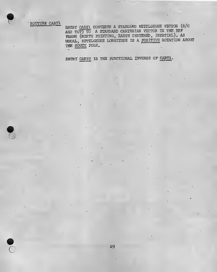
ROUTINE CARTlENTRY CARTl CONVERTS A STANDARD BETELGEUSE VECTOR (S/C
AND TGT) TO : A STANDARD CARTESIAN VECTOR IN THE BRF
frame (north pointing, earth CENTERED, INERTIAL). AS
USUAL, BETELGEUSE LONGITUDE IS A POSITIVE ROTATION ABOUT
THE SOUTH POLE.
ENTRY CART2 IS THE FUNCTIONAL INVERSE OF CARTl.

UPROUTINE ^RTl COC^eOO FTN V3.0-P308 OPT=l 08/29/72 11,32
SUBROUTINE CART1(X,Y) CART
DIMENSION X (12) ,Y (12)
SUBROUTINE TO CONVERT' Y^BET-ElrGEUSEC"1U=COS (Y (2) )
"S-iu=-mrrrr2r)CLA=COS (Y(3) )
SLA=SIN(Y(3))
Y(12) CART— "CAKrBETEL VECTOR TO PLANET CENTERED INERTIAL CART— X^A-RTTSTATl CARr
CART
X(i)=— Y(1)*CL~A‘^CM1X(2)= -Y(1)*CLA»SMUX(3) = YCTr^^L-A UttRl
X{4)= Y(7)^CLA^CMU-Y(8)^SMU+Y(9)'^SLA’CMU CART
X ( 5) ="- Y { 7) '^CLA^SMU=YT8r^Cnt3^T9T^'SUr^LJ “ CARTX(6)= ’Y(7)»SLA-Y(9)*CLA CARTx(7)-— (Y(i)+Y(4)) *CLA’*-mu~-T{5)-*sm*-y-t^r*sn*cm -CARr
X(8)= - (Y(i)+Y(4)) ^CLA^SMU-Y (5) ^CMU-Y (6)’^SLA»SMU CART
X t qr^ tTnU'+r t 4UT^SrA^T-{ 6T'nXTS CTATTr
XdO )= ( Y(7) +Y(10) ) ^CLA^CMU- (Y(8) +Y(11) ) ^SMU + ( Y ( 9) +Y (12 ) ) SLA^ CMU CART
X( 11) =- (Y ( 7) + Y ( 10) ) ^CLA^SMU- (Y {8)+Y (11) )»CMU^(Y {^T+)rfI?)T^SUA‘^ SMLTC ARTX{ 12)= ( Y(7) +Y (10) )^SLA-{ Y(9) + Y (12) ) ^CLA CARTRETURN 7“ ^CART"
ENTRY CART2 ' CART
CARTCART“CART_CARTCARTXA^TCARTXARrCARTXARrCART
Y ( 1 ) - PSS (X (1nx (2)TX ( 3nY(2) =-ATAN2(X (2) ,X(1)
)
Y ( 3
)
= AS I N ( X ('3 ) /Y ( 1) )
CMU=COS ( Y(2)
)
S''!U=STNTY'L2)")
CLA = COS (Y(3)
)
SLA = SIN (Y(3) )
Y(4)= (X(7)-X(l) ) »CLA^CMU-(X(8) -X (2 )) ^CL A»SMU+ (X (9 ) -X (3
)
Y( 5) =- ( X (7 ) -X (I )-) ’^SNU-“(X ( 8T-XTr)T»CHUYt6)= (X(7)-X(l> )^SLA'^CMU- (X (8) -X( 2) ) ^SL A'^SMU- ( X ( 9) -X(3>
Y ( 7) =Xr('4)^CXA*^CW-X(-?r^i:X7\'^0+XT6) SLAY(8)=-X (4)^SMU-X (9)^CMUY ( q
)
±-X (
4
) *S L
A
C MU“X ( 5) SL A SfTU^"XT'6')' ‘CUAY(10)= (X(IO)-X (4) )^CLA»CMU- (X(ll)-X(5) )^CLA»SMU+(X(12)-Y (11) =- (X(10) -X (4) ) ^SMU-{X (11) - X(5) )‘»CMUY( 12) = (X(10) -X (4) ) SLA^CMU- (X( 11) -X (5) ) SLA^SMU- (X (12) -
RETURN
UAKICARTCART'CARTC“ARrCARTCART
)»SLA CARTCART
)»CLA CARTCArTCARTCART
X(6))»SLA CARTCART
X{6)) CLA CART
) CLA
CARTr A D T

SUBROUTINE SETY(Y) SETY
SUBROU/lNE TO COMPUTE STATE VECTORS OF INTEREST'Y ( 1 r^IWE-Y(2)7T(iq) NAVIGATED BETELGEUSE STATEY(20r--Y•(37^-ENVIR0NME^^^-BETE^IEUSE^ST7^^EY(38 ) -Y (55) .'NAVIGATED CARTESIAN STATE

routine setyTHIS ROUTINE IS LEFT OVER FROM AN EARLY VERSION OF THE
NAVIGA.TION PROGRAM. IT HAS ONLY ONE OPERATIVE INSTRUC-
TION AND CALLS TO SETY MAY BE REPLACED BY THAT INSTRUC-
TION WHEREVER THEY ARE FOUND, IN THE PROGRAM.
AREA A CALL TO CARTl IS ONLY OPERATIVE INSTRUCTION IN ROUTINE.
LOADS BETELGEUSE ESTIMATED STATE INTO Y(38)-Y(49) AS
CARTESIAN VECTOR.
30
AUTOW
CALL CARTl (XE,Y (20)
)
OEFTNP-CARTESIAN-DIFFERENCr^EC TORCALL MAT ADD (XE,Y(38),Y(80),i2,l,2)
LOAD UPPER CART r' DEV,-- VECTOR"WIThrTSTXMATEir^ONSTflTrrCONSTRUCT PSEUOO-BETELGEUSE VECTORS FOR NAV AND ENV
otn-o—r=nT6Y(I4-91) = Y(I + 31)-Y{I + 13)XS(I) = Y(I + 37)
XS(I+6) =XE(I)•^XT(I)=Y (1 + 43)
XT tI + 6) = XF(I + 6)
CDTJTTN UT~- CALL CAPT2 (XStXCS)"CALL CART2TyT;XCrT'CONSTRUCT TRANSFORM TO LOCAL TANGENT FOR S/CCALL TBG (XCS(7) ,"XCST8Tr5<rCST9TVR'yVr)CALL MATMUL (RXVT,XCS ( 4 ) , Y ( 62 ) ,3 , 3 , 1
)
CALL"M A T MUL ( RyVTTXC S'
t'
/ ) , Y ( 59 ) , 3
,
3 , 1
)
CALL MATMUL (RXVT,XCS(10) ,Y(65) ,3,3,1)COfTSTRUCT ' TRANSFORM TO'LOCAtLn' ANTGE'NTTOR'rGT
CALL T8G(XCT(7),XCT(8), XCT (9 ) ,RXVT)CALL ’MATMUL (RXVT, XCT t~ 4TVY( 6
-
8T , 3,37-11CALL MATMUL (RXVT,XCT( 7 ) ,
Y
( 77 ) , 3 ,3 , 1
)
XDO 30 1=1,3Y{I + 56) = XCS (I)Y ( 1 + 73) =XCT (I)
CONTINUERETURN
se
routine relSUBROUTINE REL COMPUTES RANGE, R-RATE, AZIMUTH
VATION KROM A TWO-VEHICLE CARTESIAN VECTOR AND
ORTHONORMAL VECTORS. CONTRARY TO COMMENT CARD,
VECTORS NEED NOT BE NAV BASE VECTORS (SEE AREA
TINE POPOUT).
AND ELE-THREEUNITL, ROU-
31
DIMENSION Y(12) t‘ S(4>
COMMON VAROrMENSION-'VAR(56-OOr,-“P(-5t) Otr) , SAEQUIVALENCE ( VAR (60 1
)
, P,( D )
EOU-IATAL-ENCE— ,SAVE(1) )
(P(i300),BLK(l))DIMENSION REFl t3)V' REF2 (31
DIMENSION' OXierrOXNB (6) ,UR (3 )
CURRENT NAVIGATION BASE COORDINATES
no S 1=1,6m (T)=Y (If6)-^Y(Tr'
"
CALL UVEC(DX(1) ,CX(2) ,DX(3) ,UR)
s ( tr^-oarruRTOXT rnS (2) =DOT (UR, DX (4)
)
S(3) = ATAN{D0T(UR,REF3) /OOTCURTREF^")S(4)=ASIN(D0T(UR,REF1)
)
RETURN

ROUTIKE SETUPSETS UP OUTPUT FORM OF BETELGEUSE STATE,
CONVERTS LONGITUDE AND LATITUDE TO DEGREES.
COMPUTES S/C HORIZONTAL SPEED.
DEFINES HEADING ANGLE AS A POSITIVE ROTATION ABOUT S/C
RADIUS VECTOR FROM DUE WEST.
32
5 0UT(I+9J=Y(I+9) SETUP 16

\
4
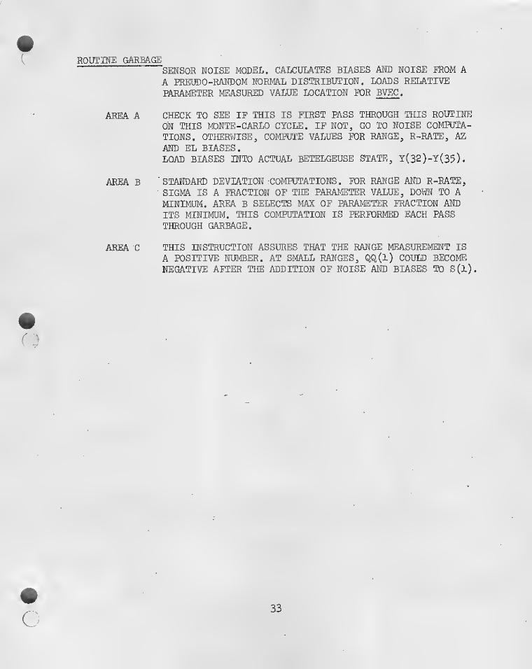
ROUTINE GARBAGE^SENSOR NOISE MODEL. CALCULATES BIASES AND NOISE FROM A
A PREUDO-RANDOM NORMAL DISTRIBUTION. LOADS RELATIVEPARAMETER MEASURED VALUE LOCATION FOR BVEC .
AREA A CHECK TO SEE IF THIS IS FIRST PASS THROUGH THIS ROUTINEON THIS M3NTE-CARLO CYCLE. IF NOT, GO TO NOISE COMPUTA-TIONS. OTHERWISE, COMPUTE VALUES FOR RANGE, R-RATE, AZ
AND EL BIASES.LOAD BIASES INTO ACTUAL BETELGEUSE STATE, Y(32)-Y(35).
AREA B 'STANDARD DEVIATION COMPUTATIONS. FOR RANGE AND R-RATE,
SIGMA IS A FRACTION OF THE PARAMETER VALUE, DOWN TO AMINIMUM. AREA B SELECTS MAX OF PARAMETER FRACTION ANDITS MINIMUM. THIS COMPUTATION IS PERFORMED EACH PASSTHROUGH GARBAGE.
AREA C THIS INSTRUCTION ASSURES THAT THE RANGE MEASUREMENT IS
A POSITIVE NUMBER. AT SMALL RANGES, QQ(l) COULD BECOMENEGATIVE AFTER THE ADDITION OF NOISE AND BIASES TO S(l).
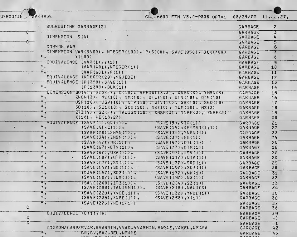
ubroutik" CtTbSOO FTN V3*0-P308 OPT=l 08/29/72
9^
SUBROUTINE GARBAGE(S)
DIMENSION S(4)
COMMON VAROT ME MSI ON' VAR t56 DOT
YdOO )
GARBAGEGAR-Bin^TGARBAGEGARBAGE"GARBAGE
, BLK(700 ) GARBAGEGARBAGE
2
T4'5'
6
T8
"EOUlTmrENCE"TTAirtl) GA-RBAGF
—
““9tVAR(401) ,NTEGER(1)
)
GARBAGE{ VAR(6Q1) ,P(Tr) GARBAGE 11
EQUIVALENCE (NTEGER(29) ,NGUIOE) GARBAGE 12EOUIVAL’ENCE' '(PT3F0r',SAVE(nT GARBAGE 13
(P(13D0) ,BLK(1)) - GARBAGE 140iMtl^rUN-GaC4T^ ErE(4T, CTIU), Rt i- H A 1 ( 3 , 3 > , XNBN(3}, YNBN(3) GARBAGE 15
ZNeN(3), NEdO), NM(iO), DTL(iO) , OTNdO) 5 OTM(IO) GARBAGE 16' uspdoirusvdo)^, OTP^ritrrTdJTVTl 0 ) r "SRTl'O ")
, SROTIT]! G AKU Abt 17SO(IO) , SCi(lO) , SC2(1Q) , NKtlO) , TLMdO) , NS (3) GARBAGE 18ZTZUr < SZC4) rTALIGNTlOTdX-NBETTT, YNBEfTrrZNBETTT GARB AGE ' 19X(18) , VIE(18,27) GARBAGE 2D
EnUiVALENUt TSAVEir) (EA VE (FTT'STGTrn GARBAGE 219
, (SAVE{9) ,C(1} )
,
(SAVE(19) ,REFMAT(ld) ) GARBAGE 22(S AV Ft 2 8 ) N3N rrT7r; rSAI/ET3T) ,YNBN (rn GARBAGE 23
*1 (SA VF(34) ,ZNBN (1) )
,
(SAVE(37) ,NE(1)
)
GARBAGE 24-*
,
- TSAVETAEJ , TSA Wr(577 iDTcrm G ARH AGE 25(SAVE(67) ,OTN{i) ), (SAVE (77) ,OTM(l)) GARBAGE 26
^ V TS AVFTBTrvU SRTrTT; TEA'virrgTT iVSTnn GARBAGE 279
, (SAVE(107) ,UTP(i) )
,
(SAVE (117) ,UTV (1)) GARBAGE 28(SAVETrZF) ,SRTTn , fEAVE (137) ,SRD (in GARBAGE 299
, (SAVE(147) ,SO(l)
)
, (SAVE(157) ,SC1(1)) GARBAGE{SAVE(1&7) ,SCr2 (ITl , “dSAVE(177y,NW(l)) GARBAGE 31
9 (SAVE(187),TLM(1)), (SAVF(ig7) ,NS(1)) GARBAGE 329
^
9TSATFrEOUTTZITClTd(SAVF(208) ,TALIGN (1 )
)
,
(SAVE C^QA) ,SZ(i))(SAVE (218 ), MALIGN)
GARBAGEGARBAGE
3334
9 (SAvr(229") tXNBEdTr; (SAVE (232) ,YNBE (1)
)
GARBAGE 359 {SAVE(235) ,ZNBE(1) > , (SAVE(258) ,X(1)) GARBAGE 36
(SAVE(276),WE(1,1)) GARBAGE 37C , GARBAGE 38
^^AGE 19GARBAGE 40GARBAGE ^41
GARBAGE 42GARBAGE 43
rrrrT'w
)
:OMMON/GARB/RVAR,RVARMIN, WAR, V VARMIN, VARA Z , VAREL , NF AMVOR,BV,SAZ,BEL,NFAMB

CHECK IF INITIAL VALUES FO BIASES HA^E BEEN SETiF^HV AR ( i-):rGT;i.VT“(io'“ro'^ ^BR = UNURN(0,NFAMB,D,,BRO)B V =UNUR NrOTNFAM B“,"0 77B VO
)
3AZ=UNURN(0,NFAMP,Q . ,8AZO)"RFL-^NU RNTirTRETTMT^VOTTETELTn
^
Y(32) = BRY C33 )" =' BVY(34) = BAZYt3BT~“=~"BELCONTINUE
GARBAGEGARBAGEGAR8“AG£'GARBAGEGA'RBAGEGARBAGEGARBAGTGARBAGEGARBAGEGARBAGETiARBAGEGARBAGE
SUBROUTINE GARBAGE CDC 6600 FTN V3.0-P308 OPT=l 08/29/72 11«32,27.
1-00
COMPUTE MEASUREMENT NOISE AND ADO BIASES B
STTTm^TTATITSITO ^ R V A R t KVTTRMTTnSIG(?)=AMAX1 ( ABS (S(2) ^VVAR) , VVARMIN)SIG(3)=VARAZ
— :
SIG(U) = VAREL B
QO(ti = sil) +" ukurn(o,nfamv;br75Ig~('ht"CO(l) = AnSlQQd)) c_
QO < 2 T '=-'SH 2 ) V KURN ( GTNFAHV , BWSIGTZO"!00(3) = S(3) + UNURN ( 0, NFAMV,8AZ,SIG (3)
)
GO ( 4 ) -S { 4)“'+‘”UNURN ( 0 , NFAMV "tBEL ^SIGTAnIF(VAR(1).LT.5.) PRINT 10 0 , 3P , 3 V , B AZ , LEL , ( SI G ( I) , 1=1 ,4)
FORMAT ( /IX V8E15-761— —
RETURNEND ^
^
GARBAGE 57
GARBAGE 58GARBAGE 59GA'RBAGE 60GARBAGE 61GARBAGE 62GARBAGE 63G'AH'B AGE 64GARBAGE ' 65GARBAGE 66GARBAGE 67U A K BAG t 68GARBAGE 69

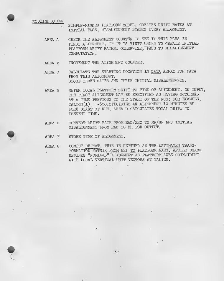
ROUTINE ALIGN' ” SIMPLE-MINDED PLATFORM MODEL, CREATES DRIFT RATES AT
INITIAL PASS, MISALIGNMENT BIASES EVERY ALIGNMENT,
AREA A CHECK THE ALIC2IMENT COUNTER TO SEE IF THIS PASS IS
FIRST ALIGNMENT. IF IT IS VISIT UNURN TO CREATE INITIAL
PLATFORM DRIFT RATES. OTHERWISE, PASS TO MISALIGNMENT
COMPUTATION,
AREA B INCREMENT THE ALIGNMENT COUNTER.
AREA C CALCULATE THE STARTING LOCATION IN DATA ARRAY FOR DATA
FROM THIS ALIGNMENT.STORE THREE RATES AND THREE INITIAL MISALIGNMENTS.
AREA D REFER TOTAL PLATFORM DRIFT TO TIME OF ALIGNMENT. ON INPUT,
THE FIRST ALIGNMENT MAY BE SPECIFIED AS HAVING OCCURRED
AT A TIME PREVIOUS TO THE START OF THE RUN: FOR EXAMPLE,
TALIGN(l) = -600. SPECIFIES AN ALIGNMENT 10 MINUTES BE-
FORE START OF RUN. AREA D CALCULATES TOTAL DRIFT TO
PRESENT TIME,
AREA E CONVERT DRIFT RATE FROM RAD/SEC TO MR/HR AND INITIALMISALIGNMENT FROM RAD TO MR FOR OUTPUT.
AREA F STORE TIME OF ALIGNMENT.
AREA G COMPUT REFMAT, THIS IS DEFINED AS THE ESTIMATED TRANS-
FORMATION MATRIX FROM BRF TO PLATFORM AXES . APOLLO USAGE
defines "NOMINAL" ALIGNMENT AS PLATFORM AXES COINCIDENT
WITH LOCAL VERTICAL UNIT VECTORS AT TALICET.
4
(
3^

...—
—
— —SUBROUTINE ALIGN ALIGN 2
Cc
ALIGNSUBROUTINE TO SIMULATE THE PERFORMANCE OF A PLATFORM ALIGNMENT ALIGN
34
c ALIGNCOMMON VAR ALIGN
56
0 1 MC^NSION VA R X5'6 OOTT“^T 0 0 ) T DTIDa rOO), Q(iOU), FIRSTYTTITtn ALIGNNTEGER(iOO), 0(100), P(5000) ALIGN
7
8
EauTVAtFNCE—rVARd) ,Y (1)) ALIGN 9
(VAP (101) ,OYOX (1)
)
(VAR (2D1)-, 0(1) )^
(VAP(30i) ,FIRSTY(1) )
(VAR (401) ,NTEGER (1) )
(VAR (501) ,0(1))(
V
A R- X IT )
DIMENSION SAV£(g50) , BLK(700), OATA(350)^ C0V(24,24)EOUrVArENCr'- {P( 350) VSAVEd) )
(P(1300) ,BLK(1)
)
( P ( 4 0 74
)
, D A T A (
1
)T"^^
(P (4424 ) ^ COV(l,l)
)
niMFNSION"13Cn’AT7”STG‘(Tr)T"CT10) , REFMAT(3,3), XN0N(3), YN0N(3ZNBN(3), NE(IO), NM(IO), OTL(IO), OTN(IO), OTM(tO)USP (10) ,
'
USV ( 10 ) ,“UTP"(iaTT"OT\r( lTr)T“SR'riO )V"SRD (TO'
SO(IO), SCl(lO), SC2(10), NW(IO), TUM(IO), NS(3)7TZ (AT'T'SZ (4) ,'“TALTGN'C10)T^NBrm",“YNBrr3')T“ZN'BETX(18) , WE(18,27):Er-rs ayfti )“,'Qcra"nT
(SAVE(9) ,C(1) ) ,
(SAVr(28) ,‘XNBN(1TTT
(SA VE (34) ,ZN8N (1) )
,
— (SAVF(47) ,NM(1) )
(SAVE(67) ,0TN(1)),—(S A V FT 8T1TUSP (TTTX(SAVE(107),UTP(1)),(SAVE{127) »SR(i) )',
(SAVF(147) ,SO(l) ) ,
{SAVF(167) ,SC2 (1))T, (SAVE(187) ,TLM(1) ) ,—(SAvr(2oo)“,ZT2('rn“i(SAVF(208) jTALIGN (1 ) )
,
"“(SAVE (2 29) ,XNBE(i) )",
(SAVE(235) ,ZNBE(1) ) ,
' (SAVF(276) ^VIE (1,1) )
" '
(SAVE(19) ,REFMAT(1,1))"( SA Vtr(3 DTYNBNTD )
(SAVE(37),NE(1))(SAVE(57) ,OTL(l))(SAVE (77),DTM(1))TS AVrF9 7)TCJSr(‘r)T(SAVE (117) ,UTV (D)(SAVE ( 137) , SRD(1)T(SAVE (157) ,SC1 (1)
)
'(SAVF(177)7NW(1))(SAVE (197) ,NS(1))TS A vrT2 04T7SZ ( 1 )
)
(SAVE (218) , MALIGN)(SAVE (232) , YNBE (T)T(SAVE (258) ,X (1)
)
ALIGN^ALIGN^ALIGN“ALIGN^ALIGN'ALIGN"ALIGNALIGNALIGN"ALIGNALIGN“At I g¥ALIGN"ALIGNALIGN"AtIGN"ALIGNTTLTGFl"
ALIGNalignALIGNALIGNALIGNTTcrALIGN'ALIGNALIGNALIGN_ALIGN“alignALIGN“ALIGNALIGN
'ALIGN

o
CJ
o
0U^’MYequivalence (Y{g8) ,0RIFT(1))
* , rDYu>rf 9 81TR ATrrrr(NTEGER{33) ,LIGN)
EQUTV7\rFNCr”TBLK‘(l)',RTCTr)(BLK (4) ,0RFT{ 1) )
TBCinryTirxaTi* (0LK-(1O ) ,UY (1 ) )
* , (BLK (f3)TUZ(l)I
PL ATFORK~H OD EC“I S ' 3-
1
AS defined below
ALIGNALIGNMalignALIGN^AriGN"
ALIGNALIGNALIGNALIG^ALIGN
DRlEt ALIGN'ALIGN
SUBROUTINE ALIGN CoC 6600 FTN V3,0-P308 OPT=i 08/29/72 11.32,27.
C ALIGN 57
ALIGN
ALIGN
ALIGN
CONSTRUCT ALIGNMENT GIASfSDO IS 1 = 1,3
--
G^IFT (I) =UNURN( 0 ^NFAMBiO. , ALIGN B)
RFFFR-INTE-GRATETr-ORTFT-TO~TrHE"3JFQr=Y(l) - TALIGN(LIGN)
ALIGN'ALIGNALIGN"ALIGNALIGN
ALIGN
CALCULATE INDEX TO STORE ALIGNMENT DATA IN ARRAYMM=(LIGN-1)»7 + "250 +-1
data (MM) =RATE(I
)
DATA (’^M + 3) =DRIPTTr) ^
ALIGNALIGNALIGN
RT(I) =RATE(I) »3600G00.20 nRFT(I)=DPIFT<I)^10G0.
MM=LTGN^7+250n'\TA/v(M»-TAi TrKiri TrM»
ALIGNALIGNALIGNALIGN

COMPUTE REFMAT AT TALIGN, DEFINED AS THE ^MINAL- GSHX= UNIT(R) rSMY= UNIT(R X V)
-
SMZ=‘TJNIT(SMX"X
CA LL UVhC'(Y rTB) , Y ( 39 ) , Y ( 4 0 ) , U XTCALL UCPOSS(UX, Y(41) ,UY)
ALL“UCR03S{UX,UY,UZ),ALL TRN <UX,UY, UZfRFFM at, DUMMY) G
ALIGNALIGNAL IGNALIGN
PRINT 100, LIGN, ( ORFT ( I)
', 1= 1 , 3) 7" (RT( I) , 1^173) ALIGNF0RMAT(/14X,2AHTHIS IS ALIGNMENT NUMBER , 15 ESH BIASES AND RATES ALIGNR- -7'5Tr^5T A L I G N
R-TURN ALIGN

ROUTINE REFCOMPUTES UNIT VECTORS OF ACTUAL LOCAL VERTICAL, ACTUALHAV BASE, ESTIMATED LOCAL VERTICAL AM) ESTIMATED NAVBASE. ACTUAL AND ESTIMATED QUANTITIES DIFFER BY PLAT-
FORM DRIFT. CURRENT NAV MSE VECTORS ARE DEFINED AS THELINE-OF-SIGHT SYSTEM, SUBROUTINE IS ALWAYS CALLED WITHESTIMATED CARTESIAN STATE,
AREA A CALCULATE ESTIMATED LOCAL VERTICAL VECTORS.
AREA A1 CALCULATE ESTIMATED LINE-OF-SIGHT VECTORS.
AREA B CALCULATE THE TOTAL PLATFORM DRIFT MATRIX, GAMP . GAMP IS
THE TRANSFORMATION FROM ACTUAL W ESTIMATEDPLATFORM AXES . LET V BE ANY ESTIMATE OF A VECTOR IN THE
'
BRF FRAME AND V* -BE ITS VALUE AFTER APPLICATION OF PLAT-FORM. ERRORS:
VECTOR IN ESTIMATEDPLATFORM FRAME
VECTOR IN ACTUALPLATFORM FRAME
DISTURBED VECTOR IN
BRF FRAME
= REFMAT-" X GAMD*^ x REFI^mT x V
(gamp X REFMAT)^ X REFMAT x V
V = REFMAT X VT? '
*"
V^ = GAMD X V-P -P
V* = REFMAT^ X V*_p
CALCULATE GAMD x REFMAT .
CALULATE (GAMD x REFMAT )^.
TCALCULATE ( GAMD x REFMAT ) x REFMAT .
AREA C APPLY THE JUST COMPUTED MATRIX TO THE ESTIMATED LOCALVERTICAL VECTORS TO GET THE ACTUAL VECTORS.APPLY THE SAME MATRIX TO THE ESTIMATED NAV BASE VECTORSTO GET THE ACTUAL NAV BASE VECTORS.
35
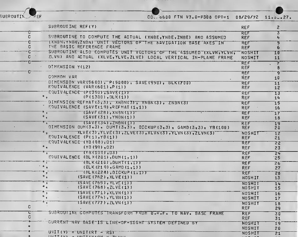
SUeROUTIK ~FF GO. o600 FTN V3«0-P3b8 OPT=l 08/29/72 11.3
SUBROUT I-NE REF(Y)
SUBROUTINE TO COMPUTE THE ACTUftL ( XNBE t YNBE , ZNBE) AMO ASSUMEDX NB-fTTY N 8 ITT? NB N ) “UKT
THE BASIC REFERENCE FRAMESUBROUT INE'ALSO COMPUTES "UNII^ECrORS Of^TKE^ASSUMEa^f)aVKyYUWZLVN) AND ACTUAL ( XL VE, YL VE , ZLVE) LOCAL VERTICAL IN-PLANE FRAME
DIMENSION Y(12)
COMMON VARn r M E NS 1 0 N' VA R'C5 6 0 0 ) V“P { BOOU), SAVE(9bU), BLK(7DinFOUTVALENCE ( VAR (601) ,P (1)
)
EOUT V ACENCE—tPfS^TTS'AVETrn(Ptl3Q0) ,BLK{1))
D I M FN S 1 0 N'-RE F M A T ( 3 ,^3 I X N'B N( 3 )'
T' TNBN ( 3 ) , Z NBN(3)
EQUIVALENCE (SAVE (19) ,R£FMAT (1,1))“(SAVF (28 Vj xNBN (rrr ^
(SAVE(31) ,YN3N(1)
)
( S A V E T’S ATT7N8NTITlDIMENSION DUM(3,3), 0UMT(3,3), DICKUP{3,3), GAM0(3,3), YBdOO)
XL V E { 3) vY LV E { 3 )“,ZLVE(3) , xL\rN'(T7"rnrvNi'3TTZi:vNrmEQUIVALENCE (P(1),YB(1))FQUIVALENCE"(Y3 (98 ) ,01)
^
(YB (99) ,02)( Y Brnr D )to37
—^
EQUIVALENCE (BL K ( 2 0 1) , OUM ( 1, 1 )
)
^
( BL K ( 2 r 0 )", DUMrriTm(eLK(219),GAMD(l,l))(BLK(228) ,OIC<UP (ITTTT
(SAVE(762),XLVE{1))TSTTVETTTEBTTYrvrcm
'
(SAVE (768) ,ZLVE(1) )
(SAVE! 771)’7XLVN(1)'J(SAVE(774) , YLVN(l) )
(SAVE (777)TZLVN (ITT
C URR Eirr-N A V B A S'E" I S"-n N E- 0F-
'
NOSHIT
REFREFREFREFREF'IREF
REFREFREFREFREFre'FREFNOSHITREFREFREFl^EFREF"REFREFREFNOSHIT"NOSHITNOSHIT"NOSHITNOSHIT"NO'S Hit
UNIT (•Y)- =-UNIT (RT - - “RSIt INt T T / V \
tiOSHTTNOSHITNOSHir
n T T / \/ kinkt
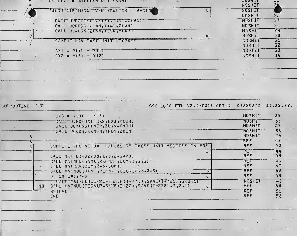
= UNlllAMbN X YNBN)
CaLCtn:ATE-LOCAL“VrRTTCAC^UNTr^EtrrO(
-* CAtr' uvECXT mTTmTTCTiTxrvfnCALL UCR0SS(XLVN,Y(4) »ZLVN)
COMPUT NAV BASF UNIT "VECTORS
OX 1“- " Y (7) --YT1 )
0X2 = Y(8) - Y (2)
NUiOi I
NOSHITfrosTarNOSHIT"NOSHirNOS HITwsTTrNOSHITTNOSHirNOSHIT“NOSHirNOSHIT
SUBROUTINE REF CDC 6600 FTN V3.0-F308 OPT=l
DX3 = Y{9) - Y(3)
CALL UCROSsTy^S^ZLVN^XNBN)CALL'"UCROSS (XNPNVYNBN VZNBNr
COMPUTE THE ACTUAL VALUES OF THESE UNIT VECTORS IN ERFg
CALL MAT(03,D2,D1,1,3,2,GAMO)CA LL“MA TMUL (GAM D ,REFM AT-^ DUM V3737DCALL MATRAN(OUM,3f3,OUMT)CALL-MATMUL(DUMT,REFHAT,OrCKUPV3r5T31 Bn'lini = i,7,3 C
--CALT' MATyurCDrCKUPTSAVrCTf / f U ) , SA VE"TTT75‘1) ,3 , 3 , IT
CALL MATMUL(niCKUP,SAVF(I + 27) , SAVE (1+228) ,3,3,1)
8/29/72 11. 32,27
NOSHIT 35-TrO'SHNOSHIT 37
““NOSHIT ^ ^38
NOSHIT 39“REF ^42
REF 43-T?ErF 44REF • 45
“REF ^46
REF 47"REF ^48
REF 49


ROUTINE P20SUBEXECUTIVE FOR NAVIA.GATION MARKS, ADVANCES COVARIANCE,
- TAKES MARK, RETURNS UJDATED STATE.
AREA A THIS AREA IS LEBT OVER FROM THE ORIGINAL VERSION AND WASNEVER ACTIVE.'
AREA B READS UIDATED VECTOR BACK INTO ARGUMANT LOCATIONS ,
;
36

COMMON VARniMPNSrON"VART5BOB'nEQUIVALENCE ( V A R (6 0 1 ) ,P ( 1 ) )
EQUIVALENCE (P( 350)-,-SAVE(l)), (P(1300) ,BLK{1)
)
• 0lMEt^I1DN-ReFMA-r(-3r3-r“X ri'S )
EQUIVALENCE (SAVE (19) , REFMAT { 1 , 1 ) )
Pr50Q0), b:AVt(9bU), BLICIAO'OT
(SAVF(258) ,X{1))'
nlMENSION'TriS)SUBROUTINE TO CONTROL THE TAKING OF A NAVIGATION MARK
P20P2 0"
P20'P20
P2GTzxrP20T2 0'
P20'P20P20
9
1011'
12"13
14

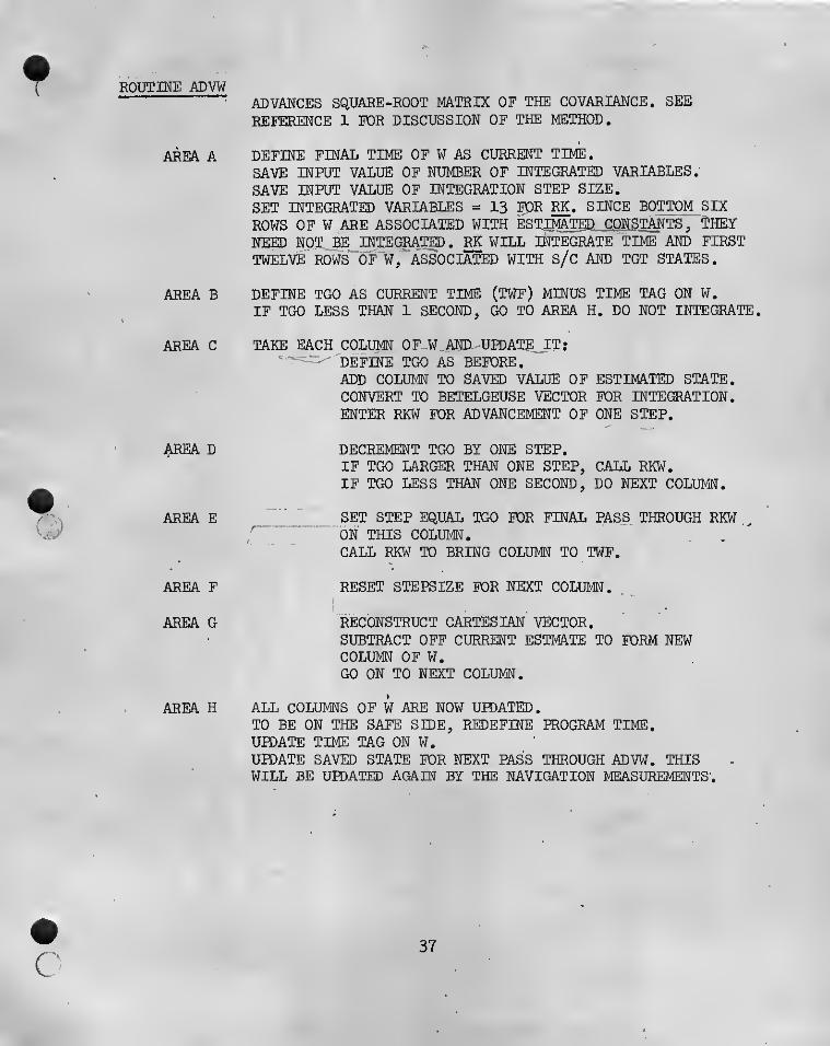
ROUTINE ADW
AREA A
AREA B
AREA C
AREA D
AREA E
AREA F
AREA G
AREA H
ADVANCES SQUARE-ROOT MATRIX OF THE COVARIANCE. SEE
REFERENCE 1 FOR DISCUSSION OF THE METHOD.
DEFINE FINAL TIME OF W AS CURRENT TIME.
SAVE INPUT VALUE OF NUMBER OF INTEGRATED VARIABLES.
SAVE INPUT VALUE OF INTEGRATION STEP SIZE.
SET INTEGRATED VARIABLES = 13 TOR RK, SINCE BOTTOM SIX
ROWS OF W ARE ASSOCIATED WITH ESTIMATED CONSTMTS .
~
NEED WOT BE INTEGRATED . RK WILL INTEGRATE TIME AND FIRST
TWELVE ROWS' OF w/ ASSOCIATED WITH S/C AND TGT STATES.
DEFINE TGO AS CURRENT TIME (TWF) MINUS TIME TAG ON W.IF TGO LESS THAN 1 SECOND, GO TO AREA H. DO NOT INTEGRATE.
TAKE EACH COLUMN OF W AND. UPDATEJiT;DEFINE TGO AS BEFORE.ADD COLUMN TO SAVED VALUE OF ESTIMATED STATE,CONVERT TO BETELGEUSE VECTOR FOR INTEGRATION.ENTER RKW FOR ADVANCEMENT OF OWE STEP.
DECREMENT TGO BY ONE STEP.IF TGO LARGER THAN ONE STEP, CALL RKW.IF TGO LESS THAN ONE SECOND, DO NEXT COLUMN,
SET STEP EQUAL TGO TOR FINAL PASS THROUGH RKW^ON THIS COLUMN.CALL RKW TO BRING COLUMN TO TWF,
RESET STEPSIZE TOR NEXT COLUMN.
RECONSTRUCT CARTESIAN VECTOR.SUBTRACT OFF CURRENT ESTMATE TO FORM NEWCOLUMN OF W.GO ON TO NEXT COLUMN,
ALL COLUMNS OF W ARE NOW UPDATED.TO BE ON THE SAFE SIDE, REDEFINE PROGRAM TIME.UPDATE TIME TAG ON W.UPDATE SAVED STATE TOR NEXT PASS THROUGH ADVW, THISWILL BE UPDATED AGAIN BY THE NAVIGATION MEASUREMENTS.
37

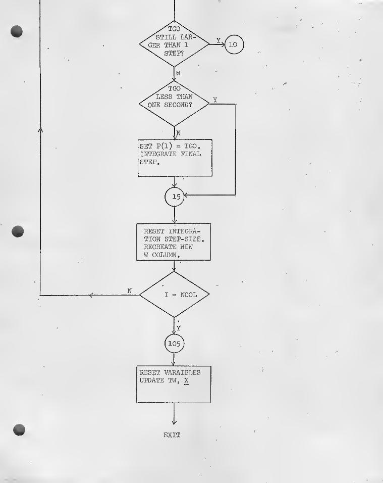

vw CDv woOO FTN V3.0-P308 OPT= 1 08/29/72 11.34_.27,
SUBROUTINE AOVW(T,XF) ADVW"ADW
COMMON VARniMEMSrON-VA-R:t5-eOO) , T(lDO)t NT EGER (1 D 0)> P (50 0 0). SAVECBBD)
BLK(70 0)
EOUI V At-E-NCE-t V A R { 1TTrCm
ADVW“ADVW
EQUIVALENC
(VAR (401) ,NTEGER(1) )
-fVATrBUlT. P d))(P( 350) ,SAVE( 1)
)
-(P(1300)-VBLKfl)T
niMENSI0N-URl(3) ,UR?(3) ,UP(3)DIMENSION 0(10), X(18), WE(18,27)'ETUIVAtETOE^S A-VTr9T7 CT CIT)
(SA VE(258) , X( 1) )
( S A V H < 2 7 6 T','WF (T, 1)
)
:OUI VAL“ENC£- (Oti) vTW)
lUPi (1) ) , (0 (5y,UR2 (1) )
(8LK{64g) ,UR(1) )
DIMENSION X0P(12) ,XF(18),XFP (12)EOUIVALENCE f BLK (1) .XOP (1) )-,TBC)Cri 3 ) ,XFP(1 j )
EQUIVALENCE ( NT EGER ( 9) , NCOL)
COL = NCOLS A VF -rURRE NT“T TKrT OT -I NrTITA R, S TEP- S IZ E, S E T I.V.=13
AOVWADVtrADVWTOWADVWADVWAOVWTDVWADVW“ADWAOVW'ADVTfADVWADVWADVW
AOVW‘ADVWAOVW'AOVW'AOVW"AOVWADVW7\DVW
8
. 910
Tl'12"13'
14
T5'16'17
18"I9‘
20
TT22'23'
24"25"
26
2728——Twm
^
^
ADVW 30NV-NTEGER ( 6)
SIFP=P(1)ADVW "Si
ADVW 32
cM b G I’ R ( 6 ) - 1 3 ^ SDI/W 33
ADVW 34GHt-CK TtO"
B"TOO-TWF-TWIf^ (AnS(TGO).LT.l.) GO TO 105 B
ADVW 35AOVW 36
c AUVANCt W BY UOLUMKjS ’ - 000 100 1 = 1,NCOL
ADVW 37AOVW 38
C1 G(j= ) Wb -
1 W
CRFATF PERTURBED STATEAOVW 39ADVW 40
DO b
5 XOP(J) = X(J) +• WE( J,I) »SQRT (COL)
ADVW 41ADVW 42
CONVERT TO 8ETELGEUSE SYSTEM_ r-LL 1 rn PT? fvnp _ Y r 7 \ ^
AOVW 43

UeROUTINF AOVW CDC 6600 FTN V3.0-P308 OPT=l 08/29/72 11.32.27,
d[/^c
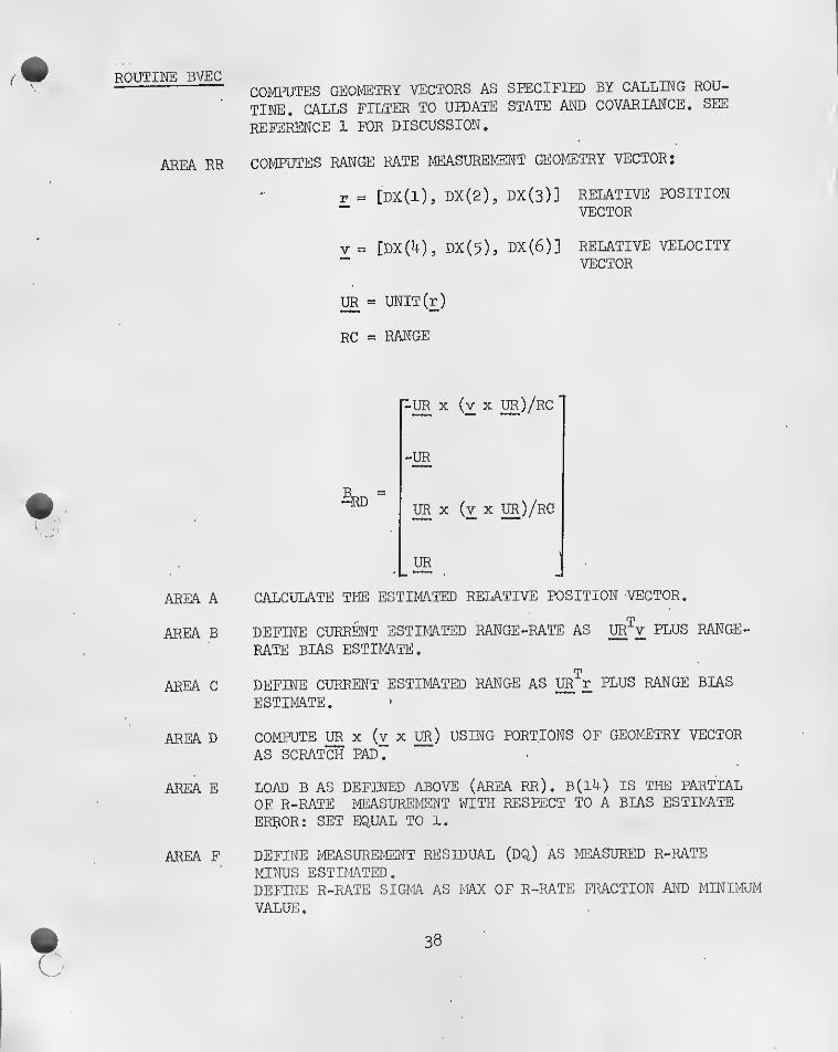
ROUTINE BVECCOMPUTES GEOMETRY VECTORS AS SPECIFIED BY CALLING ROU-
TINE. CALLS FILTER TO UPDATE STATE AND COVARIANCE. SEE
REFERENCE 1 FOR DISCUSSION,
AREA RR COMPUTES RANGE RATE MEASUREMENT GEOMETRY VECTOR;
T = [DX(l), DX(2), DX(3)] RELATIVE POSITIONVECTOR
V = [DX(4), DX(5). DX(6)3 RELATIVE VELOCITYVECTOR
m = UNIT(r)
RC = RANGE
AREA A
AREA B
AREA C
pUR X (v X UR)/RC
-UR
UR X (v X ^)/RC
UR
CALCULATE THE ESTIMATED RELATIVE POSITION VECTOR.
DEFINE CURRENT ESTIMATED RANGE-RATE AS PLUS RANGE-
RATE BIAS ESTIMATE.
DEFINE CURRENT ESTIMATED RANGE AS PLUS RANGE BIAS
ESTIMATE.
AREA D COMPUTE m x (v x I^) USING PORTIONS OF GEOMETRY VECTOR
AS SCRATCH PAD.
AREA E LOAD B AS DEFINED ABOVE (AREA RR). B(14) IS THE PARTIAL
OF R-RATE MEASUREMENT WITH RESPECT TO A BIAS ESTIMATE
ERROR: SET EQUAL TO 1.
AREA F DEFINE MEASUREMENT RESIDUAL (DQ) AS MEASURED R-RATE
MINUS ESTIMTED.DEFINE R-RATE SIGMA AS MAX OF R-RATE FRACTION AND MINIMUM
VALUE.
38

area f set measurement type flag for filter
UPDATE STATE WITH R-RATE MEASUREMENT (CALL FILTER
)
COMPUTES RANGE MEASUREMENT GEOMETRY VECTOR;
2r
AREA A COMPUTE CURRENT RANGE UNIT VECTOR.
AREA B DEFINE ESTIMATED RANGE AS IN AREA RR(c)
AREA C LOAD B AS DEFINED ABOVE. B(13) IS THE PARTIAL OF A RANGE
MEASUREMENT WITH RESPECT TO A RANGE BIAS ESTIMATE ERROR:
SET EQUAL TO 1.
AREA D DEFINE MEASUREMENT RESIDUAL AS MEASURED RANGE MINUS
ESTIMATED RANGE.DEFINE RANGE SIGMA AS MAX OF RANGE FRACTION AND MINIMUM
VALUEI
SET MEASUREMENT TYPE FLAG FOR FILTER.
UPDATE STATE WITH RANGE MEASUREMENT (CALL FILTER )
AREA E IF THIS IS A RANGE-ONLY (VHF) MARK, EXIT ROUTXNE.
AREA OP COMPUTES AZIMUTH AND ELEVATION MEASUREMENT GEOMETRY
VECTORS
:
REFl, REF2, REF3 ESTIMATED NAV BASE UNITVECTORS
.
AZ = ATAN[ (Ur'^REFS ) / (UAeF^ ) ]
EL = asin[ur^refi 3
THESE DEFINITIONS ARE NOT UNIQUE, BUT THEY MUST BE THE
SAME AS THOSE IN SUBROUTINE REL.
39
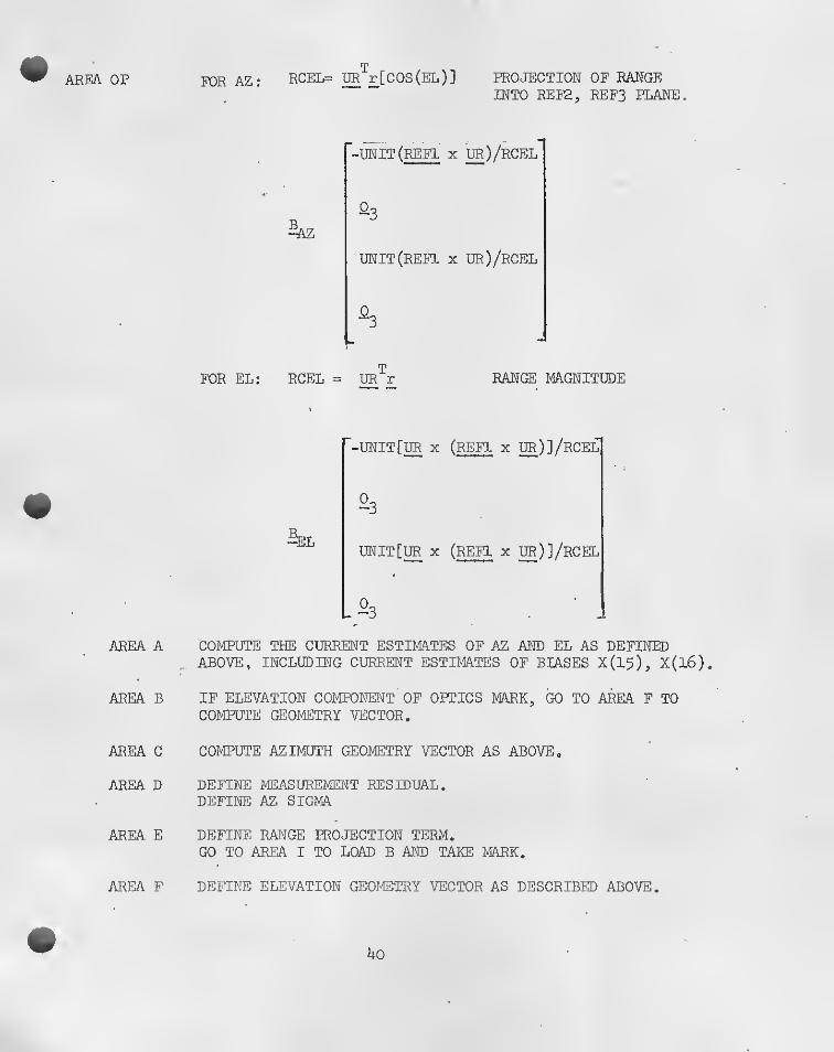
AREA OP FOE AZ
AREA A
AREA B
AREA C
AREA D
AREA E
AREA F
RCEL= UR^r[COS (EL)] PROJECTION OF RANGEINTO REF2, REF3 PLANE.
4z
'-UNIT (REFT X 1®)/RCEL
O3
UNIT(REF1 X ur)/rcel
%
FOR EL: RCEL = UR^r RANGE MAGNITUDE
r-UNIT[^ X (reFI X TO)]/RCEl|
^LUNIT[UR X (REFl x UE)]/rCEL
COMPUTE THE CURRENT ESTIMATES OF AZ AND EL AS DEFINEDABOVE, INCLUDING CURRENT ESTIMATES OF BIASES X(l5), X(l6).
IF ELEVATION COMPONENT' OF OPTICS MARK, GO TO AREA F TOCOMPUTE GEOMETRY VECTOR.
COMPUTE AZIMUTH GEOMETRY VECTOR AS ABOVE.
DEFIIJE MEASUREMENT RESIDUAL.DEFINE AZ SIGMA
DEFINE RANGE PROJECTION TERM.GO TO AREA I TO LOAD B AND TAKE MARK.
DEFINE ELEVATION GEOMETRY VECTOR AS DESCRIBED ABOVE.
4o
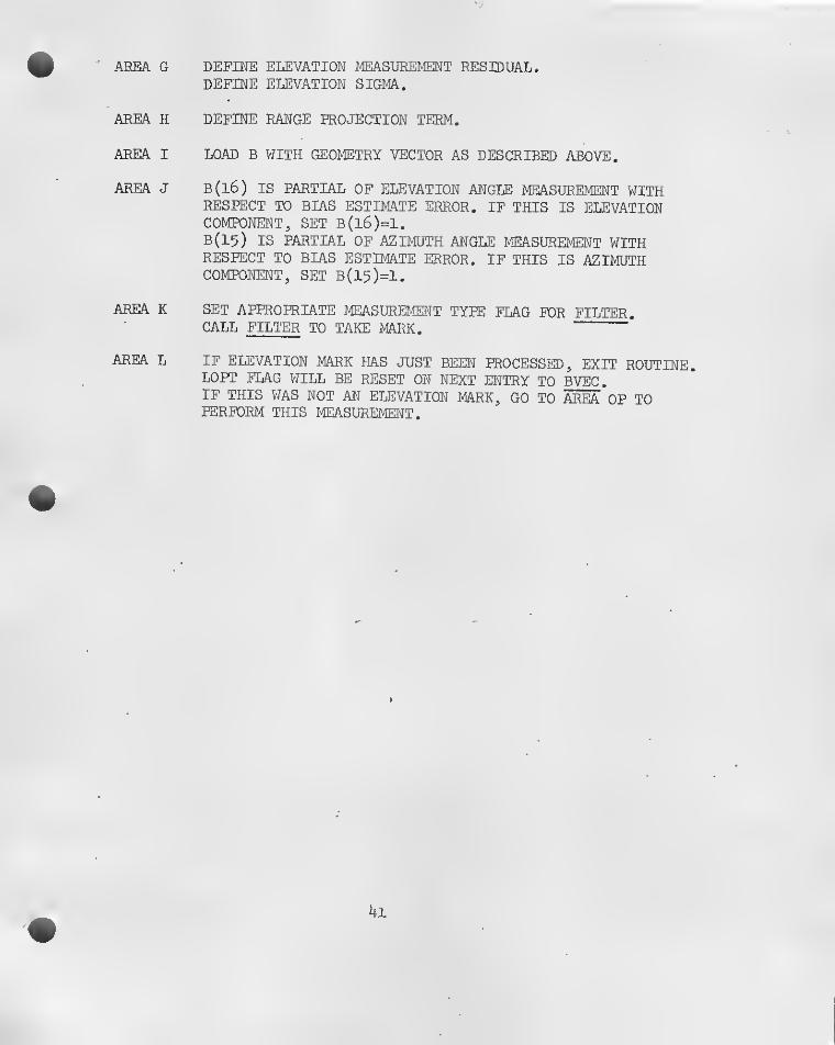
AREA G DEFINE ELEVATION MEASUREMENT RESIDUALDEFINE ELEVATION SIGMA.
AREA H DEFINE RANGE PROJECTION TERM.
AREA I LOAD B WITH GEOMETRY VECTOR AS DESCRIBED ABOVE.
AREA J B(i6) is partial OF ELEVATION ANGLE MEASUREMENT WITHRESPECT TO BIAS ESTIMATE ERROR. IF THIS IS ELEVATIONCOMPONENT, SET B(i6)=1.B(15) is partial of AZIMUTH ANGLE MEASUREMENT WITHRESPECT TO BIAS ESTIMATE ERROR. IF THIS IS AZIMUTHCOMPONENT, SET B(15)=1.
AREA K SET APPROPRIATE MEASUREIOTT TYPE FLAG K)R FILTER.CALL FILTER TO TAKE MARK.
AREA L IF ELEVATION MARK HAS JUST BEEN PROCESSED, EXIT ROUTINE.LOPT FLAG WILL BE RESET ON NEXT ENTRY TO BVEC.IF THIS WAS NOT AN ELEVATION MARK, GO TO AREA OP TOPERFORM THIS MEASUREMENT,
4l

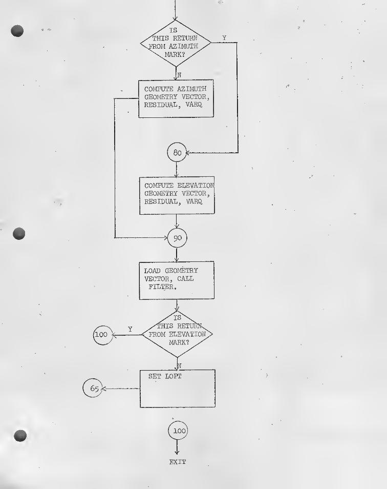
EXIT
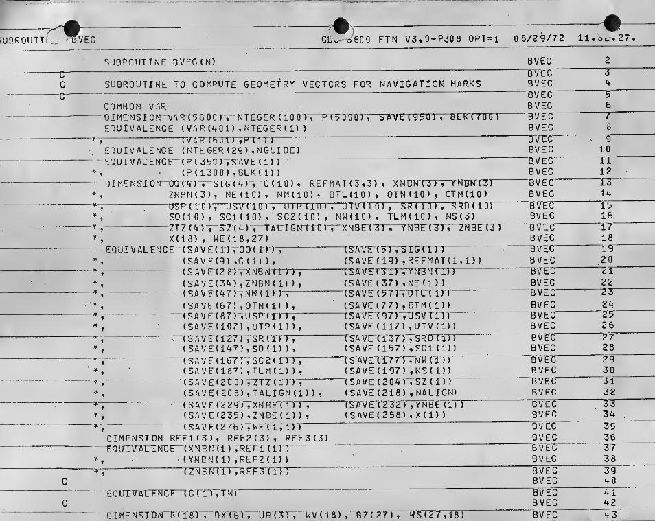
UBROUTI Ci:,.-'o'600 FTN V340-P308 OPT=l 08/29/72 ll.ot.27
S!J8R0UTINE 3VEC(N)
SUBROUTINE TO COMPUTE GEOHETRY VECTORS FOR NAVIGATION MARKS
COMMON VAR0 1 ME NS 1 0 N -VA R-( 5 6 0 (n-,“NTEGER 110 0), P’
EQUIVALENCE ( V A R (40 1 ) , NTEGE R ( i)
)
TV AR- r6 OTrrPTITOEQUIVALENCE (NTEGER (29) ,NGUIDE)EQUIVAL'ENCE- (P ( 390 )-,S AVE (1 )
)
(P (1300) ,BLK( 1)
)
0IMENSI0N"QQ(4)-^SIG(4) , 'C (TO ) , RETZNBN(3) , N£ (10) , NM(iO)
,
^ us-p-cr (T) i cDvuiPdO)SO(IO) , SCKIO) 1 SC2(10) ,—ZTZ (VTT'SZTA) V TATTlGNTtOrX(18) , WE(18,27)
EOUrVAt-EMCE -TSAVEd) , QQ(1)^
(SAVE(9) ,C(1) ) ,
(S A V Fr(2 B-)VX NB N (I'm
(SAVE(34) ,ZNBNd) ) ,
( S A V E ( 4 7 ) im ( 1 )^
(SAVE(&7) ,OTN(l) )
,
(SAVF{87) iUSP (l)“n(SAVEdOZ) ,UTP(1) ) ,
“T5 AVFd27) rSR d) "H(SAVE(147) ,SO d) ) ,
{ s A V F ( 167 r; 3 c 2 ( r))"^
(SAVE(187) ,TLM(i) )
,
(SAVE(2tI0) ,ZT7d)(SAVE(208) ,TALIGN(i) ) ,
AVT( 2 2 90TXN B F (nr;(SAVE(235),ZN8E(i))
,
{ 5 AT/ E ( 2 7 6 ) ; WET 1‘, 1 ) 1
DIMENSION REF1(3), REF2(3)» REF3(3)HauT)rALrNCE~-(XNBN(i) ;refi (in
(YNO.Nd) ,REF2(1) )
TZNBT^rnTRFFsrn'i
BVEC
DTL(IO) , DTNdO) , OTMdO), UlVdU), SKdOJ, SRUdlNWdO) , TLMdO) , NS(3)
T'7NBr(n”r^NBF (7T;^ZNBri
(SAT/ETCnTSTGCrr^(SAVEdO) ,REFMAT(1,1))('SAVErTXTTTNBMrTn(SAVE(37) ,NEd))(SAVE(57)^0TU( II)
(SAVE(77) ,DTMd))(SA7FT g7)--,1JSV I lO )
(SAVEdl7) ,UTV(1))T SA VE"(1 37 ) “,‘S RDTIT) ^
(SAVE (157) ,SC1 (D)^(S-AVETiTZOTNWTD)(SAVE(197) ,NS(1))
^(SAVE(204),SZd))’(SAVE (218) ,NALIGN)(s-AT/ rr23?)“rYN betiT)(SAVE(258) ,X(1) )
EQUTVALTNCn{C (n^TW)
niMFNsioN^BTie) d OX ( 6)7 r R ( 3 )"nwn(TarrnB'2'(T7Tr^T2'7"7raT

(BLK(l) ,8(1))(BLK(19),0X(1))
E
AiVEC 453VEC 46^
(BLK'(25") ,aR (ID(BLK(28),VARQ)
r JVEC"
3VEC 4o(nLK('29) ,TIQ)“
(BLK (30) ,NXNS)BVEC 49BVEC 50
\Ul_tN \OiJ \ i. J I
(BLK(4g) ,BZ( 1 )
)
(BLX (76) ^WS (ITT
CnMffON/BV/RV?\R,“RVARMI N", WAX
BVECBVE(^BVECBVEC’BVEC’BVEC
UBROUTINE BVEC COC 6600 FTN V3,0-P308 0PT=1 08/29/72 11.32.27
LnPT=0 BVECriui
'"
7 O 10(5,35,65,35) NBVEC 58BVEC 59BVEC 60BVEC 61BVEC 62BVEC 63BVEC 64BVEC 65BVEC . 66BVEC 67BVEC 68BVEC 69BVETC 70BVEC 71BVEC 72BVEC 73BVEC 74BVEC 75BVEC 76BVEC 77BVEC 78BVEC 79

SUBROUTINE BVEC CPC 6600 FTN V3^D-P308 OPT=l
CHECK IF THIS WAS A VHF MARK OR SECOND PART OF RADAR MAf
K
CN-TFO 7?T~GirTti~lTrUCJNTTNUECOMPUTE RELATIVE'STATE: F0R"'0PTICS"MARK'00 7 0 1 = 1 1
6
DX(T)=X(I+6) - X(I)
08 / 29/72 11 . 32 . 27 .
BVEC
BVECBVEC^BVECBVEC
iSiJc i L tr-tJvtc-toxf 1)»
Dx~t7TTnyrr)~rDCOMPUTE CURRENT AZIMUTH ESTIMATE ^ A
A-^C = ATAN(00T (UR',*?EF3) /dot tUR,REF2TT'/® rr5TCOMPUTE CURRENT ESTIMATED ELEVATION .ELC=ASIN(DOT(UR,'REFi)) + XdET— 'A'
CHECK IF. ELEVATION COMPONENT IS CURRENTLY BEING PROCESST tr0pr; e avi i—
g
cr-ra" sti 'B~
COMMUTE AZIMUTH GEOMETRY VECTOR C
CALL UCPOSS(REFl,UR,Btl))- C
OFFINF VARO, OQ AND PRO JECT ION. TERM D
DO = 00(3) - A2C—
-
VARQ=VARAZ»^2 P_
R0FL = 00T (UR,-DX tl-))^C0S(ELC) E
LOAD R ANO INCORPORATE MARKGO TO 90CONTINUEOEFINE ELEVATION GEOMETRY" VECTORCALL UCROSStREFl ,UR,B (4)
)
C ALT-tJC R 0 CSC URVO T4UT3'T IT ) FOIFINE VARQ, DO ANO PROJECTION TERM G09 = 00(4) - ELCVARQ = VAPEL^*2 G
nEL = OOT (UR,OX { 1) )
' H
90 CONTTNUE I
LOAIJ B
DO 95 1=1,3- 9(1)=-B(I)/RCEL
0(H-3)=O3(H-61 = -B(irB ( I + 9 ) = Q .
95”9(I + 12)=0.9(1+15) =0. I
I^ tLOPT,EG.l)’ B ti60’=l. J
IF(L^PT.EQ.O) B(15)=1. J
I- (LOPT.EO.l) NINS=4 KI^ (LOPT^fq.O) NTNS=3 K
' CALL' FILTER !
CHECK IF THIS WAS THE AZIMUTH COMPONENT OF THE OPTICS Ml
IF{LOPT.EQ’,ll GO’TO' lOd L
1
L0PT=1GO TO
! 100 CONTTNUE L
BVETTBVECBVEC"BVECBVEC’BVEC
BVECBVEC_’B V EC"BVECBVEC“BVEC

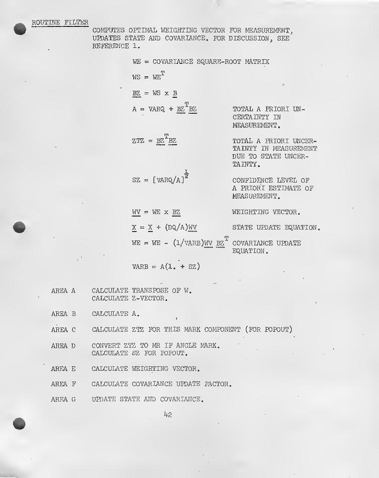
ROUTINE FILTERCOMPUTES OPTIMAL WEIGHTING VECTOR FOR MEASUREMENT,UPDATES STATE AND COVARIANCE. FOR DISCUSSION, SEEREFEREI'ICE 1.
WE = COVARIANCE SQUARE-ROOT MATRIX
WS = WE^
^ = WS X B
A = VARQ +
ZTZ =
sz = [varq/a]
W = WE X BZ
X = X + (dq/a)w
WE = WE - (1/vAEB)W^VARB = A(1, + SZ)
TOTAL A PRIORI UN-CERTAINTY INMEASUREMENT,
TOTAL A PRIORI UNCER-TAINTY IN MEASUREMEH^TDUE TO STATE UNCER-TAINTY.
CONFIDENCE LEVEL OFA PRIORI ESTIMATE OFMEASUREMENT,
WEIGHTING VECTOR.
STATE UPDATE EQUATION
COVARIANCE UPDATEEQUATION.
AREA A CALCULATE TRANSPOSE OF W.
CALCULATE Z-VECTOR.
AREA B CALCUTATE A.I
AREA C CALCULATE ZTZ FOR THIS MARK COMPONENT (FOR POPOUT)
AREA D CONVERT ZTZ TO MR IF ANGLE MARK.CALCULATE SZ FOR POPOUT.
AREA E CALCULATE WEIGHTING VECTOR.
AREA F CALCULATE COVARIANCE UPDATE FACTOR.
AREA G UPDATE STATE AND COVARIAtICE.
42
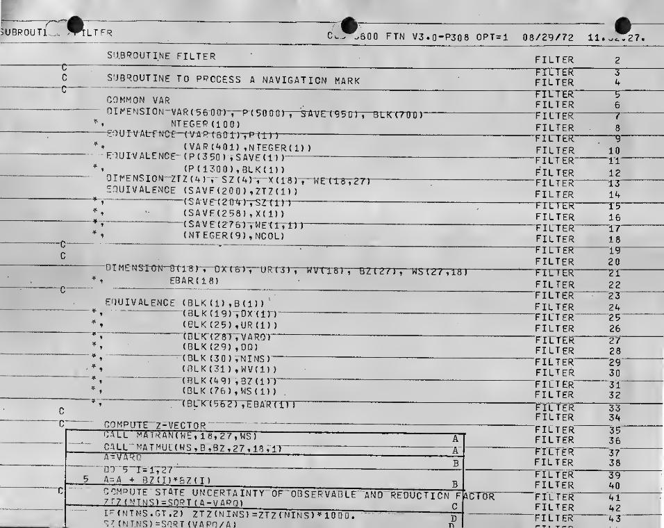
iUBPOUTl ltfr Cu.^ .600 FTN V3.0-P308 OPT=l 08/29/72 11. .^27,
SUBROUTINE FILTER
SUBROUTINE TO PROCESS A NAVIGATION MARK
COMMON VAR0 1 ME N S 1 0 N“V A R (B 6 0 {n“,—p-( 'SB trOI , 5 A
NTEGEP (100)E'TU IVAL-fNCE—(-VA f^t6'0'lr)'rPiim
(VAR (401) ,NTEGFR(1) )
EOurVALENCE- (P(350) tSAVEd))(P(1300),BLK(1))
aiMENSI0N --2TZ(4) .i- SZ ( 4) ,' X (
18)--SOUIVALENCE ( S A V F ( 2 0 0 ) , ZT Z ( 1 )
)
(^ A-V E- ( 2B -4)-
',-SZTirU(SAVF(2S8),X(1))(SA-VE{276~)-VWE-('m-rr-(NTEGER(g),NCOL)
-OtlBr—OXtBUTEBAR(18)
EQUIVALENCE (BLK(1> ,B(1))'
(BLK(ig) ,DX (in(BLK (25) ,UR(1)
)
(D.LX(?8) ,'VARO}—(BLK(29),00)
“(BLK (30) tNINS)"'(nLK(31),WV(l))(BLK{49) ,37(l)r(BLK (76) , WS (1)
)
“•{ B CK-(5'67T7E BART
C0MPUTE”7-VECT0RC-'iLL MAT^AN'( WE, 18, 27, WS )
— ^CALL 'MATMUKWS, B,BZ, 27, 18.1) AA-VAPQ ^m '5^'r=T,”27
' — —A-A + BZ(I)^BZ(I)
Tn
COMPUTE STATE U N CERTA INTY" OF ' OB SEP V AB LE ‘"AND REOUCT I ON FZTZ (NTNS)=SnPT ( A~VAPQ) qrR{NTNS.GT.2) ZT Z (N INS ) =ZTZ ( NIN5 ) ^ 1 0 D 0 .
'tT
S7 (NT,NS)=S0RT (VAPO/A)
FILTER
FILTERnUTER'FILTERFILTER-FILTERTITTER-FILTER'FILTERFILTERFILTERFILTERTICTER-FILTERTIETER-FILTERFILTER-FILTER
FILTERFILTER-FILTERFILTERFILTERyrm^FILTERFILTER"filterFILTER"FILTERTTCTWFILTER"FILTERFILTER‘FITTER-FILTERFILTERFILTER
FILTERFILTER'
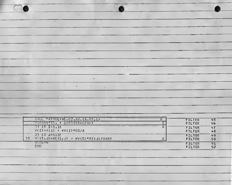

-oPfajS

6.0 REFERENCES
1. EVERYTHING YOU ALWAYS WANTED TO KNOW... (ENCLOSURE)
2. BATTIN, R. H.,ASTRONAUTICAL GUIDANCE, NEW YORK, 1964
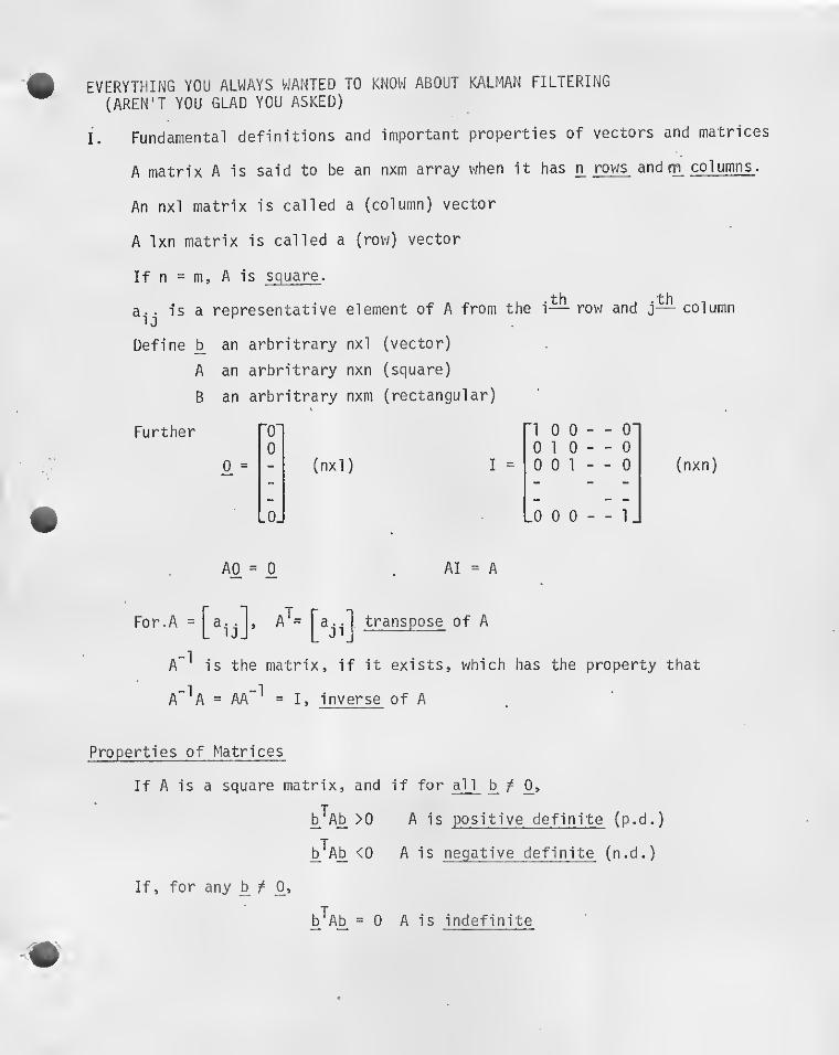
EVERYTHING YOU ALWAYS WANTED TO KNOW ABOUT KALMAN FILTERING
(AREN'T YOU GLAD YOU ASKED)
I. Fundamental definitions and important properties of vectors and matrices
A matrix A is said to be an nxm array when it has n rows and m columns .
An nxl matrix is called a (column) vector
A Ixn matrix is called a (row) vector
If n = m, A is square .
a. . is a representative element of A from the i— row and j— column^ 0
Define b an arbritrary nxl (vector)
A an arbritrary nxn (square)
B an arbritrary nxm (rectangular)
(nxn)
Further"0" ’10 0--0-0 0 1 0 - - 0
0 = - (nxl ) I = 0 0 1- - 0
. 0. .0 0 0 - - 1 .
AO = 0 AI = A
For. A = ^
A"^ is the matrix, if it exists, which has the property that
A"^A = AA~^ = I, inverse of A
Properties of Matrices
If A is a square matrix, and if for al
1
b f
^^A^ > 0 A i s positive definite { p . d.
)
^^A^ <0 A is negative definite (n.d.)
If, for any ^ 0^»
b^Ab =0 A is indefinite

2
If A = A is symmetric
a'^= A'^ a is orthogonal
If A, B are square
(AB)^ = bV(AB)"^ =.B"^A"^
Properties of Vectors
If for a set of nxl vectors
i
The are said to be linearly independent . If there are n members of
the set the set is complete with respect to the space of nxl vectors.
If the set {b.[ is independent and complete, any arbitrary nxl vector, e,
may be expressed as
e =^c.b.
Given two vectors, b^0yC_f^y if
=0 ^ and £ are orthogonal
If
b^b =1 b is normal
Eigenvalues, eigenvectors, functions of a matrix
If there exists a set of vectors and corresponding numbers X
such that
Aki =^ jki
_L^. is said to be an eigenvector of A corresponding to eigenvalve X..
If A is definite (^‘A^ f 0 for all ^ it has no = 0;
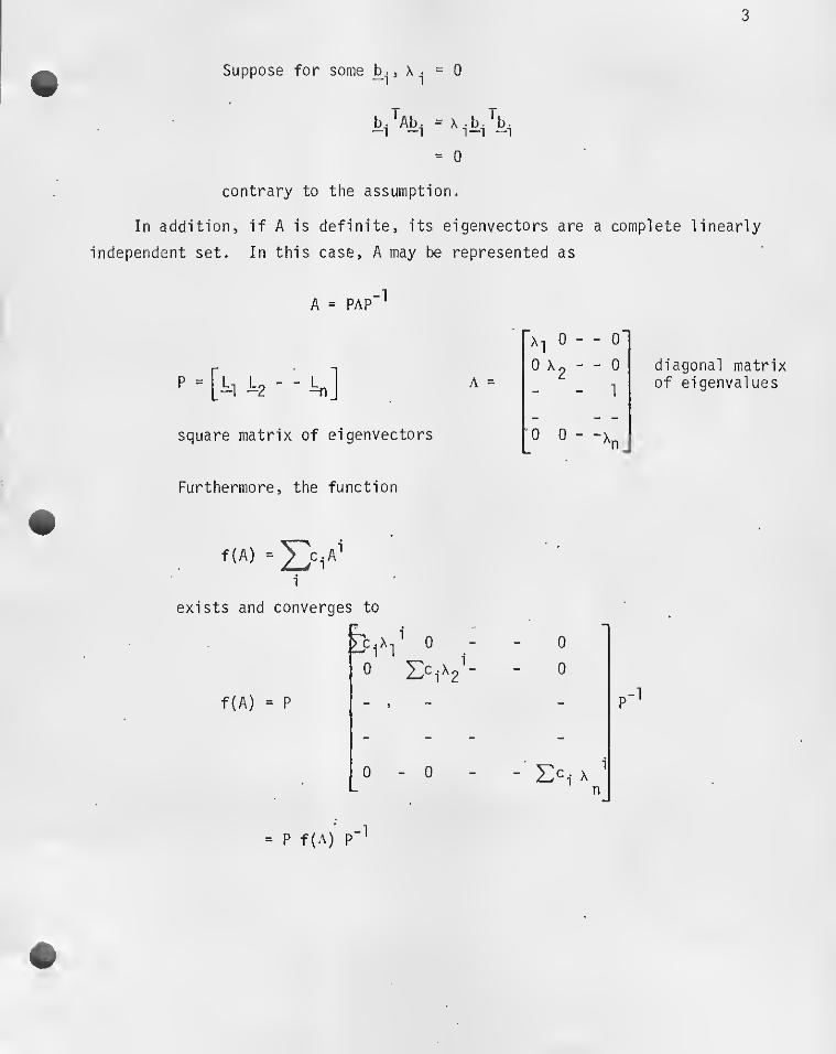
3
Suppose for some s ^^
- 0
bfAb. =x.bJb.
= 0
contrary to the assumption.
In addition, if A is definite, its eigenvectors are a complete linearly
independent set. In this case, A may be represented as
A = PAP
A =
X1
0 - - 0
0 Xp - - 0 diagonal matrix
Tof eigenvalues
square matrix of eigenvectors 0 0 ~-X,
Furthermore, the function
f{A) =
exists and converges to
f(A) = P
0
0
I- 0
= P f(A)p""'
i
Xn
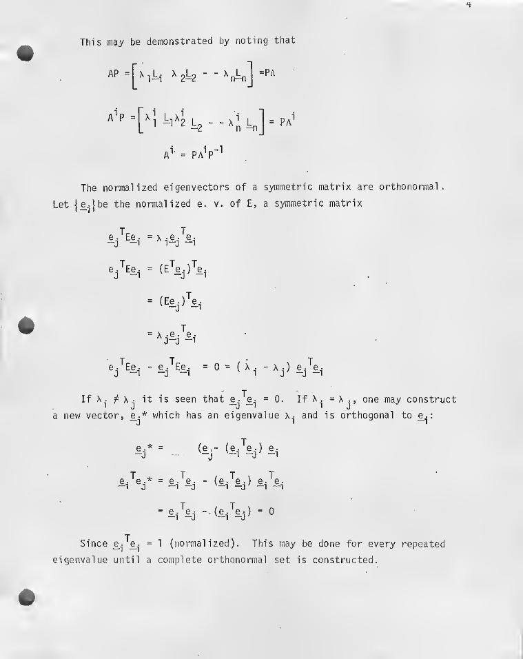
4
This may be demonstrated by noting that
AP ^ 2“2" "
aV k]><l k2“ “
a''' = pa''p"^
The normalized eigenvectors of a symmetric matrix are orthonormal.
Let |l^}be the normalized e. v. of E, a symmetric matrix
e/Ee. =
- (Eej)'e.
e. Ee.:e. -e. eg. =0 = (X. -Xj) Gj e.
If X. X . it is seen that =0. If X. =x one may construct
a new vector, £.* which has an eigenvalue x^ and is orthogonal to :
J* *
(e,- (e. e.) e.
= -(£i\j)
= 0
Since ==1 (normalized). This may be done for every repeated
eigenvalue until a complete orthonormal set is constructed.

Conventional usages in vector and matrix calculus
Differentiation with respect to a scalar:
= A -
Differentiation with respect to a vector:
nxl vector
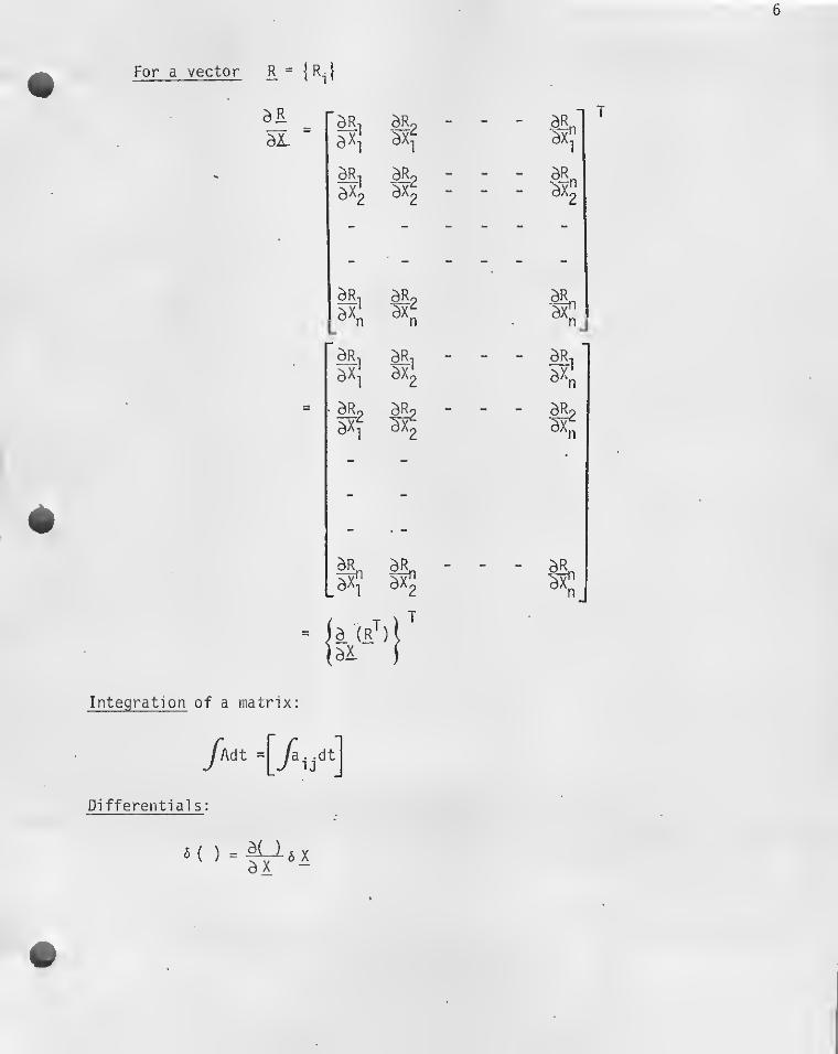
For a vector |R^}
Differential s
:

7
Examples:
5 5 X
si
6R = ^ax
6 X
III. Eyeball statistics
Let X be a discrete random variable with sample described by
the distributionjX.|
Average of X = X = jj- ^ X.
i
Variance of X = var (X) = o
^
“li X]
^ .(X^--X)
i
Standard deviation of X =ax= j^var(X)j
If X is a continuous variable, the distribution is characterized by
f(^), the probability per unit interval that X = In this case,
CO
X = y?f(Od?
CO
Var(X) =/( { -X)^ f(f) di— CO

For the vector X, a joint distribution function is defined f(|_)
1=/ if(l) - - d?^
COV(X) = [(1-A)(1'A)^] covariance matrix of X
= /(M)(i-I)^ f(i) d£2 - - df^
^x-j ‘^^1^2
<T 2
^l^n
^2^n
where - covariance of x., x.
= f(i) d$^d?2 - - di^
V
If ff =0, X. and x. are said to be linearly independent in theXiXj 1 J
statistical sense. It does not imply general functional independence .
The function
is called the correlation coefficient of x. to x.I J

y
For physical systems, covariance matrices are virtually always
positive definite.
Let ^ ^ ~ L
E = ^7 = COV (X)
E is symmetric:
eT = ee \ ^ ee= E
P‘ = P
The matrix of normalized eigenvectors of E is orthogonal, i.e
-1.
Since E is symmetric, its eigenvectors are orthogonal.
Some properties of determinants thrown in for good measure.
|A| / 0 if b^Ab /O for all b 0
a’’’I
=IA I
|a-1= |a|-i
If |AbJ = I All B
I
If P is orthogonal, |P| = +1
1 = (i| =|pT
p| =|pT||p|
, |p|2
|p|= +1

10
The determinant of a matrix is the product of its eigenvalues
= PAP
= PAP
-1
-1
= P A.-1
=I Pll p A
=I
A
-X^X2 X|^
IV. Statistical State Estimation
Some Philosophical Remarks on the Nature of the Problem
It Is worth noting that from a physical measurement point of view,
such quantities as the position and velocity of a particle are not avail-
able to direct observation. They are abstract mathematical constructs,
evolving according to an empirically developed law and should not be con-
fused with "real" aspects of the system. They are useful only in so far
as they serve to predict the observables of the system, i.e. scalar quantities
such as distance, angular measure and speed; the onl
y
aspects of the system
to which the measurement process has direct access.
Mechanics considers a system "noise free" if it is possible to argue
that, in principle, all that is needed for a perfect state determination
is a perfect sensor. In addition, the assumption is usually made in solving
particular problems that the "equations of motion" are perfectly known. In
most engineering problems, neither of these assumptions is true. Even were
they true, a further practical difficulty arises in the attempt to find the
"state" variables as a function of the observables, as the observables are
generally transcendental functions of thestate variables and time, and
therefore not amenable to algebraic solution.
The problem in state estimation is therefore two-fold:
1. Circumvent the mathematical difficulties associated with deter-
mination of the system state in terms of the observables, and (2) do so
in a manner with reflects the imperfect character of the measurements and
knowledge of the system law of motion. In order to do this, the attitude
will be adopted that the measuring device is an inseparable part of the
system in the dynamic sense: its properties effect the determination of
the system state.
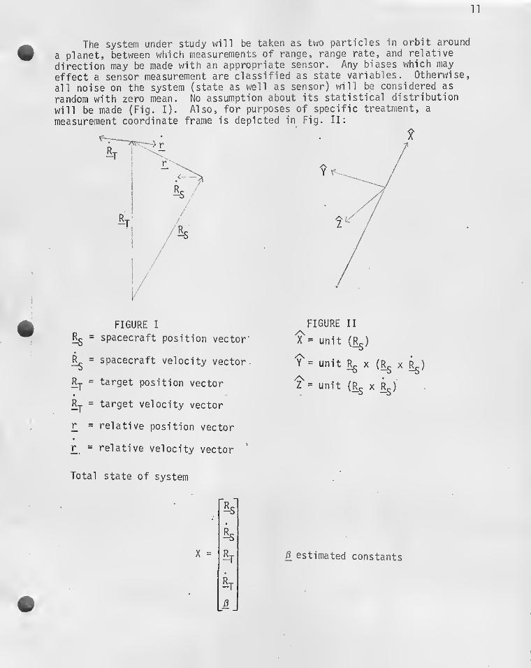
n
The system under study will be taken as two particles in orbit around
a planet, between which measurements of range, range rate, and relative
direction may be made with an appropriate sensor. Any biases which may
effect a sensor measurement are classified as state variables. Otherwise,
all noise on the system (state as well as sensor) will be considered as
random with zero mean. No assumption about its statistical distribution
will be made (Fig. I). Also, for purposes of specific treatment, a
measurement coordinate frame is depicted in Fig. II:
FIGURE I
Rg = spacecraft position vector'
^ = spacecraft velocity vector
-
Rj = target position vector
R;^ = target velocity vector
r_ = relative position vector
r = relative velocity vector'
Total state of system
-s
^T
%
FIGURE II
unit (^2)
'?= unit Rg X (Rg X R^)
Z = unit (R^ X Rg)
X estimated constants
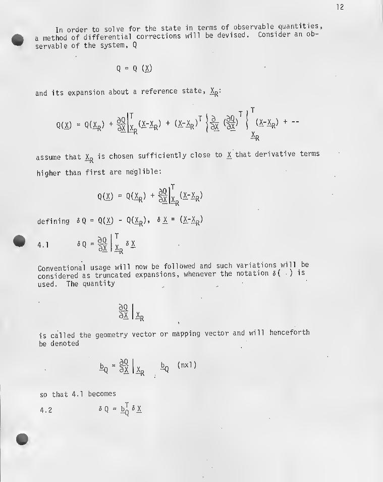
12
In order to solve for the state 1n terms of observable quantities,
a method of differential corrections will be devised. Consider an ob-
servable of the system, Q
Q = Q (X)
and its expansion about a reference state
assume that is chosen sufficiently close to X that derivative terms
higher than first are ne'glible:
Q(X) = Q(X,)
defining 5Q = Q(X.) - Q(Ar)»
4.1
T
Y
Conventional usage will now be followed and such variations wi 11 be
considered as truncated expansions, whenever the notation 6( ) is
used. The quantity
ax
is called the geometry vector or mapping vector and will henceforth
be denoted
^ =ixlxf, ^
sp that 4.1 becomes
5 Q = ^4.2

13
Equation 4.2 is the desired linear relationship between the observable Q
and the state X_. As there are n elements of 6X. determine, n independent
measurements, 5 Q, will be required. Since these cannot normally be simu-
ltaneously obtained, it will be necessary to investigate the time history
of 5 X. For gravitational field, the derivative, X. ® vector function
of X:
4.3 4x 1
for example, in the Keplerian case with ^ as previously defined
4 4 ^ X = ^dt- dt
4'
k
% X
_l _
0 I 0 0 iSi j 1
40 0 0 0 k
0 .0 0 I 0 %
0 0 --3
1
0 0 At
0 0 0 0 0_ 0
0 = [0] 3 x 3
I = I3x 3
If X and its derivatives with respect to state elements and time are
continuous, the operations and 6 ( ) are interchangeable, i.e.
dt ( )
Taking the variation of 4.3
4 . 5a 5 (^^X) = = 5 (f,(X)) = 6X = RX
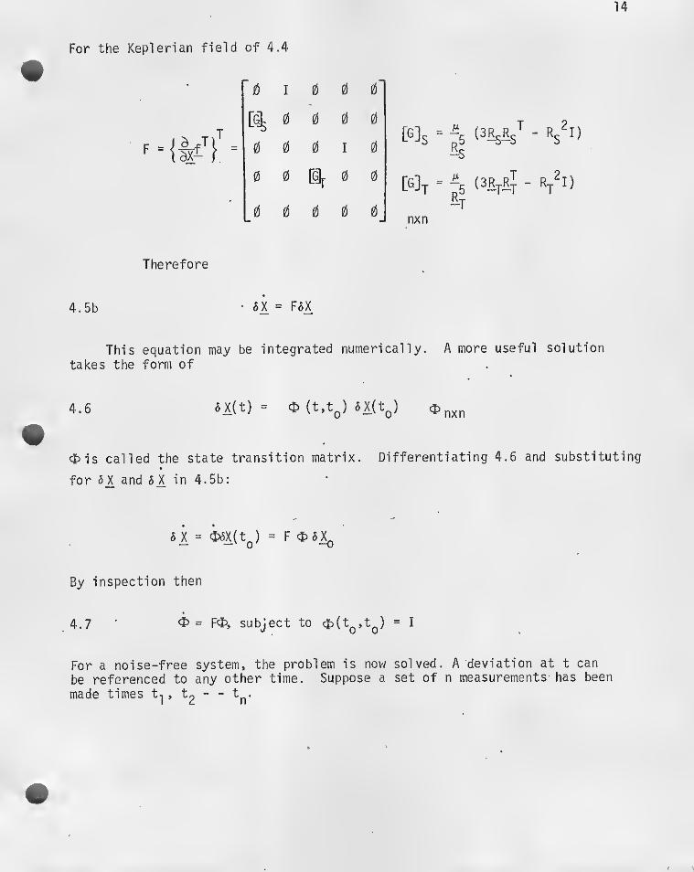
14
For the Keplerian field of 4.4
Therefore
4.5b
jS I 0 ej 0
[G^ 0 0 0 0
0 0 0 1 0
0 0 [G]j. 0 0
0 0 0 0 0
- 6X = Fax
[G]s=-5 (SRs^s^
-
h
[G]t = ^5(3R^r{ - r/i)
nxn
This equation may be integrated numerically. A more useful solution
takes the form of
4.6 6X(t) = $ 6X(t|^)
^is called the state transition matrix. Differentiating 4.6 and substituting
for a X and a X in 4.5b:
ax = iax(tQ) = F
By inspection then
.
4.7 = F<I>, subject to '5^{tQ»t^) = I
For a noise-free system, the problem is now solved. A deviation at t can
be referenced to any other time. Suppose a set of n measurements has been
made times 't-] > "^2 "^n’
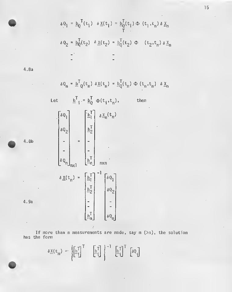
15
T
6Q2=^(t2) 5 X(t2) = ^(t2) C>
4.8a
If more than n measurements are made, say m {>n), the solutionhas the form
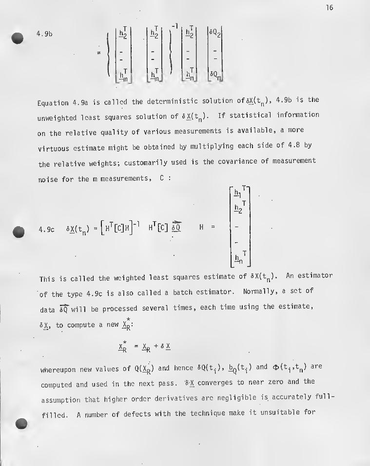
16
4.9b ,
-1
6 Q2
.. - -
- - - -
. h^ h"L-m_ L
Equation 4.9a is called the deterministic solution of5^(t^), 4.9b is the
unweighted least squares solution of 5^(t^). If statistical information
on the relative quality of various measurements is available, a more
virtuous estimate might be obtained by multiplying each side of 4.8 by
the relative weights; customarily used is the covariance of measurement
noise for the m measurements, C :
4.9c «X(t^) = [h'''[C]h]‘^ h'^[C] H
This is called the weighted least
of the type 4.9c is also called a
data ^will be processed several
*
6 X^, to compute a new X^:
T
squares estimate of 5X(t^). An estimator
batch estimator. Normally, a set of
times, each time using the estimate.
*+ 5 X
whereupon new values of Q(A|^) and hence 5Q(t^), 'i' (t-j j'tp)
computed and used in the next pass. U converges to near zero and the
assumption that higher order derivatives are negligible is accurately full
filled. A number of defects with the technique make it unsuitable for

17
many applications: all data from a set of measurements must be stored, as
well as the H matrix, which may become quite large; a large matrix inversion
is required which is slow and sometimes numerically difficult or inaccurate;
in most cases, several "passes" are needed for complete convergence. For
these reasons, a technique of sequential estimation has been developed,
which avoids these problems, as will be seen. First, an investigation into
the propagation of state errors is required.
Let Xr- be an estimate of X. Then-X
Since it has been found tHat
6X(t) =<t)6X(t^)
then
and
e(t) = ax^(t) -'6X(t) - «x(to)]
Furthermore
4.10 E(t) = e(t)e(t)'^ = *e(tg)e(tp)^ 4.^ = E(t^)
Demonstrating the evolution of the covariance of state errors. An nxn
symmetric matrix may be expressed as the sum of n linearly independent forms
of the kind

18
E = WW^
By inspection of 4.10,
E(t) = W(t)W(t)’'’ = ‘frECtg) = <}> W(tQ)W(tjV
4.11 W(t) = t W{t|^)
Physically, W is a set of linearly independent vectors drawn from the sample
space of E which have the property -that
n
IE '‘^l
V -
That is, a finite, discrete sample from a continuous distribution, having
the particular property that their simple average produces the covariance
defined by the distribution function f(0* They "typify" the distribution.
- Sequential Estimator (Kalman Filter )
The sequential estimator has the form
(5Q(t^) - &^' {\))4.12
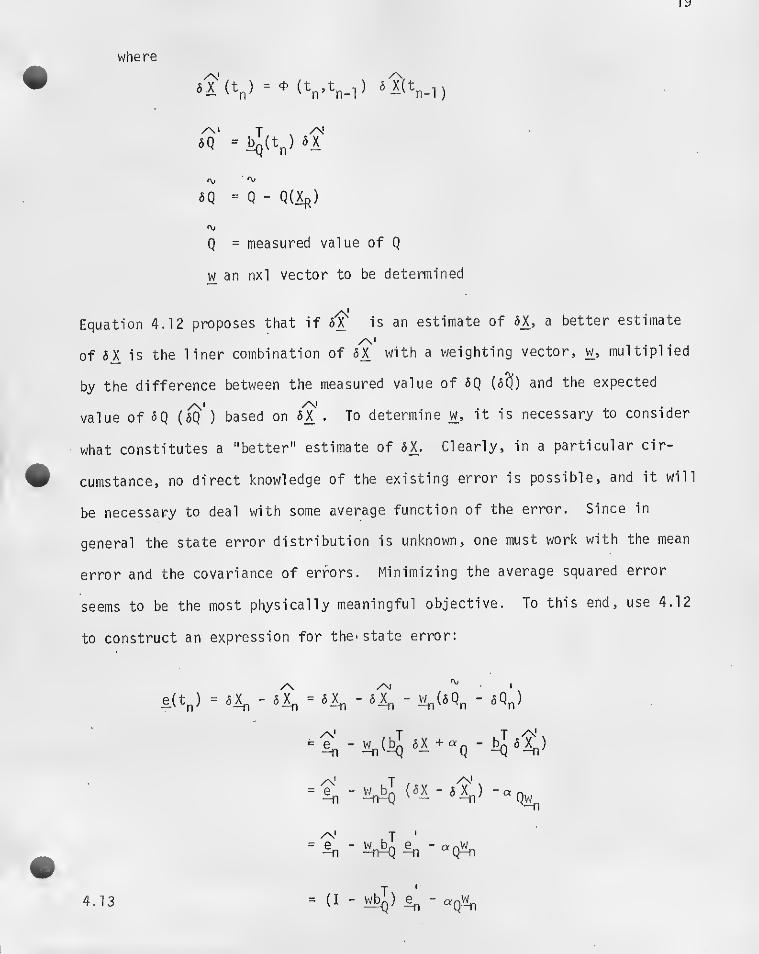
where
I y
6Q = b,i(t,) 5X
a.
«Q = Q - Q(4)
'\j
Q = measured value of Q
w an nxl vector to be determined
Equation 4.12 proposes that if SX is an estimate of 5X, a better estimate
of 5X. is the liner combination of 5X with a weighting vector, w. multiplied
by the difference between the measured value of 6Q (6?!) and the expected
value of 5Q (6Q ) based on 6X . To determine w, it is necessary to consider
what constitutes a "better" estimate of 6X. Clearly, in a particular cir-
cumstance, no direct knowledge of the existing error is possible, and it will
be necessary to deal with some average function of the error. Since in
general the state error distribution is unknown, one must work with the mean
error and the covariance of errors. Minimizing the average squared error
seems to be the most physically meaningful objective. To this end, use 4.12
to construct an expression for the- state error:
e(tj = ^4 - 5^ = 6)^ - - w„(6Q„ - sqI)—
n
n
/\
= 4-4^5 («X -5%)
= 4 - 4^4 -“q4
= (I - Wb^) 4 - aQ44.13

20
Where
f\,' IV
5Q = Q(X) - Q(4)
= Q(X) +«Q - Q(X,,)
= measured value of 5
Q
and
aq = random measurement noise
By direct calculation, the covariance of state errors E is
E = ee' = /T uT\ 6 e^(I - wbl)^ www^(I " ^ Q
—
”
- (I - ^) (I -
4.14a
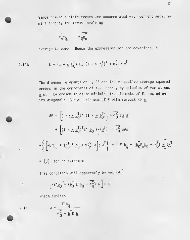
21
4.14b
Since previous state errors are uncorrelated with current measure-
ment errors, the terms involving
-n Q,ct ‘
average to zero. Hence the expression for the covariance is
E = (I “ w (I - w +“n ^
The diagonal elements of E, E' are the respective average squared
errors in the components of Hence, by calculus of variations
w will be chosen so as to minimize the elements of E, including
its diagonal: For an extremum of E with respect to w
6E = ( - 5 W ^E' (I - w + aq aw /
{+ 1(1 - ^ (
-E'^ +
-aw^)j +“ 2 T
Qw5w
E% + (^e;^ + wj 5w'
= [O] for an extremum '
This condition will apparently be met if
which implies
“q + b^E'b
4.15 w

22
This is the Kalman Filter. It remains to show that extremum of E
for which w has this value is a minimum:
Using the expression for6E:
5 ^E = ^q) 5^5^^)
It is clearly apparent that
+“q) > 0
always since E' is positive definite. Further more, the diagonal
terms of 5w 6 w^ are positive for all real variations, aw. The
corresponding second variations of E, those of the mean squared
error, are therefore positive and minimum. Figure III presents
an operational flow chart of the filter.
)^(t). )^(t), E(t^)
E'
w _E'(t) ^
+ b^E'b
t
5X'
/\
.
= b^5;x'^Q'
update covariance to present time
compute geometry vector
compute weighting vector
compute estimated deviation
compute estimated 6 Q
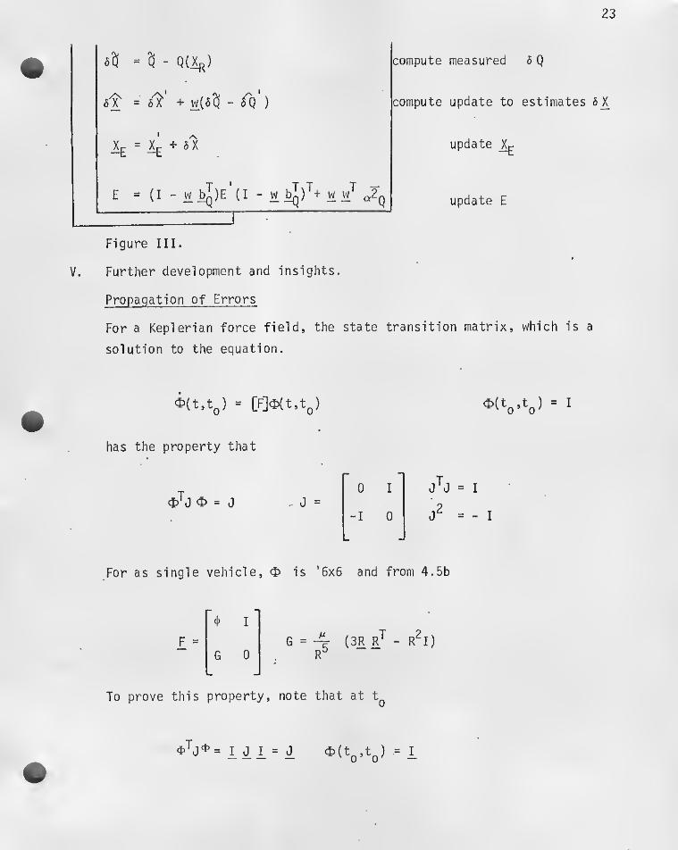
23
V. Further development and insights.
Propagation of Errors
For a Keplerian force field, the state transition matrix, which is a
solution to the equation.
has the property that
J =
cI>(to.to) = I
0 I
•I 0
- I
- I
For as single vehicle, cj) is ‘6x6 and from 4.5b
G = “4 (3R “ R^I)
To prove this property, note that at t^
F =
4> I
G 0
= X j X = j = X

24
Evaluating
= 4>+ 4»'*'jF<P
IIrj + iE
"o r 'o I "-I o"
p'fj =-
G 0 -I 0“1
CDO1
Therefore + A f,“' [^]
^ ((t^^J't*) = [O] => 4'^J4> = constant = J
Now note that lil= 1 and' therefore
For a Keplerian field the propagation of E is described by
E(t) = <t.E(tg).4>'^
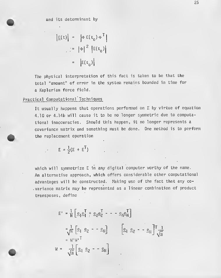
25
and its determinant by
lE(t)| = |<t. E(tjj)t'''j
,
=
The physical interpretation of this fact is taken to be that the
total "amount" of error in the system remains bounded in time for
a Keplerian force field.
Practical Computational Techniques
It usually happens that operations performed on E by virtue of equation
4.10 or 4.14b will cause it to be no longer symmetric due to computa-
tional inaccuracies. Should this happen, it no longer represents a
covariance matrix and something must be done. One method is to perform
the replacement operation
E = i(E + e'^)
which will symmetrize E in any digital computer worthy of the name.
An alternative approach, which offers considerable other computational
advantages will be constructed. Making use of the fact that any co-I
variance matrix may be represented as a linear combination of product
transposes, define
T
Vn

26
^ = W ^
and rewrite equation 4.15 as
W == (—2 T
«Q
Equation 4.14b, the update equation for E, requires careful
consideration:
Substituting for w:
Wz b‘
= (I - =
W'z= (W -
-) ww’’’ (I -W'z T W'zz^W'^ 2
)' + — aq
2 T“Q
+ Z i (“q+
T z z^W'^ W'z z''^W'^ -TT
) (W'T - Ef= ) + rf^-= an
7 7T
7 zT Z J 2z z ^ ^ an
w (I - —) (I - —
)+ — ^
2 T 2 T ^ T“Q A A '^Q ^ A ‘^Q ^ '
2^ ^ ^ (1^2) Z z"*” (ag= W {I - £: + 3;: + ^f=
y—
aq + /a (aq + a^a)^ Uq + a\)^
/i
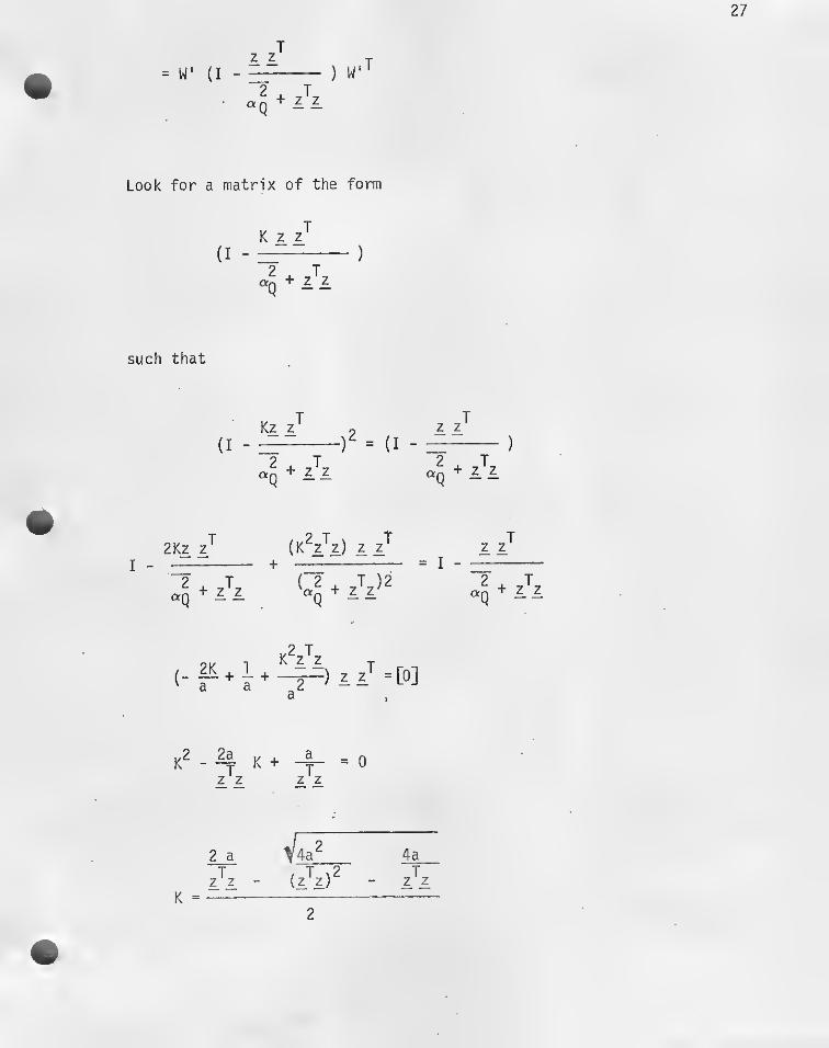
27
= W‘ (I -z z
2 Taq + LL
) W.T
Look for a matrix of the form
K z z'
(I - —
)
such that
(I -Kz z
2 + z'^zQTq + ^ Z
r = (I ’Z Z
^A
2Kz z
I -
4 ^
{K^^z) zz}^
z^
(-f
K^ - K + = 0
z z z z
44a‘
K =
2 a
- izW4a
2

28
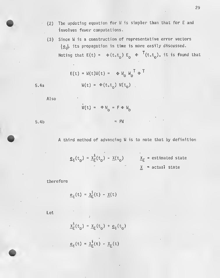
29
5.4a
5.4b
(2) The updating equation for Vi is simpler than that for E and
involves fewer computations.
(3) Since W is a construction of representative error vectors
its propagation in time is more easily discussed.
Noting that E(t) = 4>(t,t^) E^ ^ '''(t,t^), it is found that
E{t) = W(t)W(t) = * Wp 4>
W(t) = 4.(t.tg) W(to) .
Also'W(t) = = F Wq
= FW
A third method of advancing W is to note that by definition
=4(t^) - X(t^)
therefore
e.(t) = Xj(t) - X(t)
Let
4(to) =4(t„) + e.{t^)
^ = estimated state
X = actual state

30
where ^(t) and ^(t) are the respective vectors at to integrated
to time t. This constitutes a more exact solution to the problem
of propagating E and makes no linearizing assumptions as were made
to obtain 4.5b, which is the basis for equations 5.4a and 5.4b.
Definition of the Reference State
For practical purposes, the reference state is generally taken
to be the estimated state at each instant. In this case
6 r = A* - 4
= A'- °
^ <5 ^' = 0
Q (Ar)
= - Q ( X'
)
6X = = W (f! - Q (i'))
X = A' + ^A
This definition guarantees that as the differential correction
process occurs, ^ is sufficiently close to X so that the linearizing
assumptions of Sec. IV are valid.
Computation of the Geometry (^) Vecter
For a range measurement
= [iKj-r

31
r T 1 ” T r T 1 T6r = 1/2 [r VJ (5r jr) + 1/2 [L l\ t ^H) + )3
M - 1/2
5 j:+ (3
^
Where i3^ is the range measurement bias, and ^ = unit (^]
'-t T0 0
/S
X for ^ = 0
0 0
1
For a range-rate measurement
• .T-r = r r = — r
6r^ •
6 r +— 6r +)3;
— r 2 (X*5X)+— ^X +/3p
1 r ‘ />!' . /Ot ,= f I
X - (xx) X ^X + ^ 5X + 0:
= --J:^X ^ ^ X)j
^^ X + X ^X ^ P
Therefore
,

32
The geometry vector for range-rate is accordingly
b* =
[r X (2 X r)]
-9
X (t X r)]
4 “r
k:
For azimuth and altitude measurements, defined according to
Fig. II as
.1 i LAZ = TAN (t:—
Y . r
EL = SIN"'' (x • r)
Some tedious algebraic hack produces
- (x X r) /I
X X r|^
0
^Z (x X r) /^ |2X X r
0
h.1
0
0
1
0
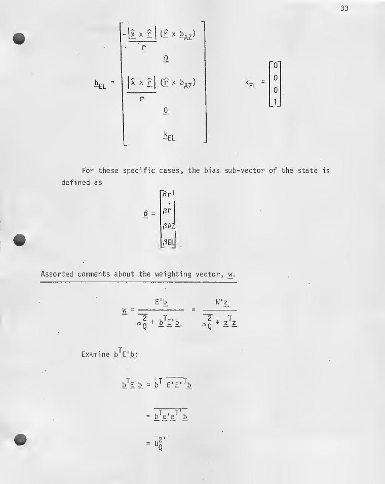
33
For these specific cases, the bias sub-vector of the state is
defined as
] 0 r
0 -pr
Pki
/3EL
Assorted comments about the weighting vector, w.
E’b W'zw =
«Q+ 2 T
aq ^ 1
Examine b^E'b:
b'^E'b = b^ E'E'^b
— b'^e ' e"^ b

34
where = Uq, the a‘ priori uncertainty in Q due to state errors.
”2Since IS the variance of Q due to measurement noise, the term
aq'*'AZ.
is the total variance of Q due to measurement noise and states
uncertainty. Now compute the estimate 6Q, the estimate of 5Q
based on 6x:
5? = S^'+w (sE! - 6Q'
)
6Q = ^ 8r + b_^W ( 5 ?! - 5Q' )
= 6Q' +b'’'wz
Q
(5?i - 6Q')
= 6Q' +z^z
2 +orQ
^
(5?! - s'q')
2 2'
^ + [r<^Q
- Tq')

35
Finally
/N ^ ,
5Q = 6Q‘
Let the ratio of measurement noise to state uncertainty be denoted
so that
“) + 5 ^
q:q+ Uq
<x
«Q =«Q' ( -WQ ( t. )
Obviously if measurement noise variance, , is very small
20
compared to the state uncertainty of 6Q, Uq, we have p' 0 and
5Q^5Q estimate equal to measured
On the other hand, if the measurement noise is large compared to the
state uncertainty 1/p' ~ 0 and
'
:estimate equal to previous estimate
Now look at the reduction of the state uncertainty of 6Q, Uq,
resulting from a measurement. From 5.3

36
by definition
W = W‘ {I - z z')
2 ^ ,,2a - aq + Uq
cac = 1
= b'^WW^b
_ kTu *T T\ i.iiTi
b'W (I - z z‘) (I - z z') W 'b
ca ca
= b^W (I - z J
= Z.^ (I - Z 1
= ug'd -
"d “»
"r 'Tf?"
'

37
Again, as noted before, if p' 0»
0
i.e. the state uncertainty of 6Q is greatly reduced. If the
measurement noise is large compared to the state uncertainty,
p7(1 + p' 1
This tallies with the expectation that if the measurement process
is very noisy compared to the state errors, the average state errors are
little reduced by the fixes. The case of a range measurement is particu-
larly illustrative:
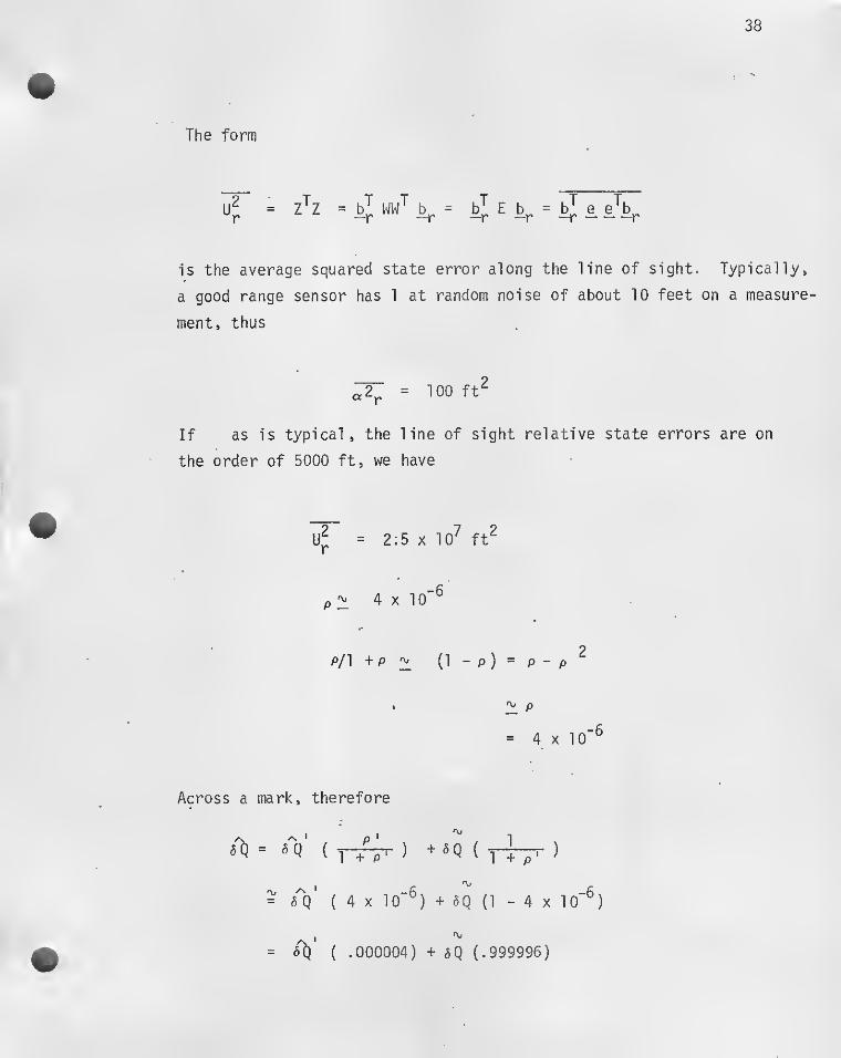
38
The form
U2 = Z^Z =bJwwTb^= =
is the average squared state error along the line of sight. Typically,
a good range sensor has 1 at random noise of about 10 feet on a measure-
ment, thus
= 100 ft^
If as is typical, the line of sight relative state errors are on
the order of 5000 ft, we have
= 2;5 X 10^ ft^
4 X 10"®
2p/1 +P2i (l“p)==p-p
’ ^
= 4x10'®
Across a mark, therefore
= A' ( ) +^Q( t4t^ )
= 613 ( 4 X 10"®) + 5q (1 - 4 X 10"®)
t
^ 6^} ( .000004) + 6Q (.999996)
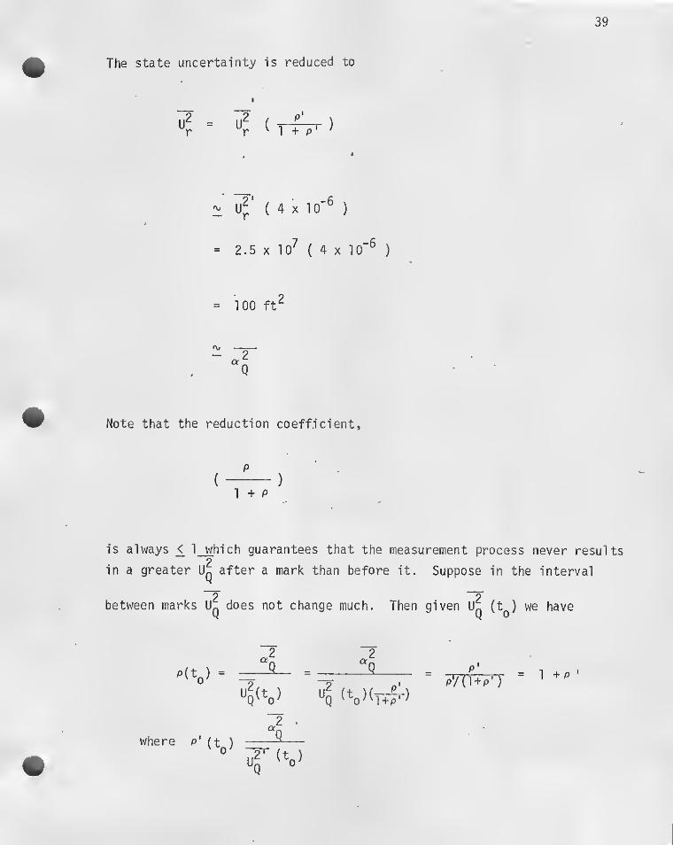
39
The state uncertainty is reduced to
Ur
U^' ( 4 X 10"®)
= 2.5 X 10^( 4 X 10‘®
)
= 100 ft'
Note that the reduction coefficient,
1 + P
IS always j< l_which guarantees that the measurement process never results2
in a greater Uq after a mark than before it. Suppose in the interval
~~2 ~2between marks Uq does not change much. Then given Ug (t^) we have
a. aP(t^) = =1 5.
7/~{}+p'j= 1 +P
a.
where p* (t )
Uq

40
If, by assumption, p changes little between marks, after n marks
p(t^) - p(to) = 1 + p'(t,)
p{t^) - 1 +P'(t.) = 1 + 1 +p' = 2 + p'(tj
P(t„)'- (n + 1) + p'Uq)
thus'(^
0 ^
1 +^(to) 1 + n+1 + p'-Tt^T
1 n + 1 » 1
And
I.e. the uncertainty in the direction of ^ is not much reduced
after a large number of marks. When this condition has occured, the
filter is said to be “saturated". Since E is a real symmetric matrix,
it eigenvectors are orthogonal, and the matrix of its normalized
eigenvectors is an orthonormal matrix. Hence, as noted in Sec. I, E
has a diagonal representation in terms of its eigenvalues as
E = P A PT
ppT
=pTp _

The matrix of orthonormal vectors, p , may be considered as defining
a co-ordinate rotation in the space of n dimensions; or alternatively,
a change of variable in that space, to a new set
41
f = P^6X
Cast w into the new variables
P^Eb= P w
^2
“Q - ug
pTpPP^b
A
T“Q
bj = Pi
» Note that
K =pT Aa = _M
“i hi
A1 so
— i

42M= ~
OL. + E51
( If )'
Where is the i^*^ eigenvalue of__E, the variance of ^ . In,2 ^
that <r. >> o-j for allj
and er
^“q the inverse in brackets
(w^ )
-V
aQ
The updating equation in terms of the new variables is
6? = P 6X = p 6XT ^
I
+ P^W { 6 Q -)
I
^I
= af +w (6Q - 5 Q )
the event
approximates 1
43
For the case where = 0 as described previously, the update for the
i— component of 5^ is
as expected. Thus thus true meaning of w is this:
It's sort of the inverse partial of X. with respect to Q, weighted
by assorted variances of the measurement and state uncertainties,
and conditioned by the extent to which ^.is in the direction of
the expected error; sort of . . .
?,9
13 j;'^0
/ rovReiidezvous Analysis
2. 9.1 Introduction
Concentric Flight Plan is the name given to the technique of rendez-
vous developed during Program Gemini and now in use for Apollo. It is the
fruition of attempts to construct a plan which offers simplicity of opera-
tion, high reliability of achievement and fuel economy. As a matter of
basic philosophy, it has been assumed that the spacecraft crew would par-
ticipate in the rendezvous activities to the ext^'nt of flying the vehicle,
evaluating the progress of the trajectory and (when necessary ) computing
backup solutions for the maneuvers.
Early studies by Flight Procedures Branch and others resulted in the
identification of transfer elevation angle ) and transfer interval
) as critica!L parsmieters characterizing the shape of various intercept
trajectories. Further work resulted in choices of wt and ^j^p, to reconcile
conflicting requirements of fuel economy, error propagation and ease of
operation. As a logical extension of this work, the coelliptical trajec-
tory was settled on as the standard pre-transfer condition. Since the
time of arrival at a given elevation angle can be varied by changing dif-
ferential altitude in the coelliptical phase, it is possible to control the
transfer time for a given , placing it so as to satisfy requirements
of lighting, navigation, and ground tracking. By fixing ’?,p| and cot in
advance and choosing a coellipticai pre-transfer condition, the shape of
the rendezvous trajectory is held constant throughout from various approaches,
so that the crew can hope to become familiar with its development during
training. Such familiarity enables them to monitor its progress, detect
off-nominal conditions and develop a high degree of proficiency in execu-
tion. The predictions of digital analysis and simulation v;ith regard to
trajectory behavior and fuel consumption appear to have been borne out
in detail on the Gemini and Apollo programs.
A principle activity of Flight Procedures Branch during Projects Gem-
ini and Apollo has been the construction and testing of rendezvous maneuver
charts. These are provided as an independent source of rendezvous maneuver
solutions, requiring only the most fundamental information - range, range
rate, elevation angle - available directly from the radar and platform.
In order to perform the required analysis and verification, several .large
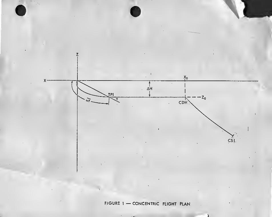
2
digital programs capable of solving for vari-eus maneuvers and providing
dispersed trajectories have been constructed. Among the original techni-
ques developed may be noted. the derivation of maneuver functions for TPI
and CDH, and the iterative use of the Clohessy-Wiltshire equations to com-
pute transfer maneuver.
2 . 9.2 Development of Concentric Flight Plan
2. 9 . 2.1 Transfer Phase
In order to clearly display the relative motion of the rendez-
vous trajectory, solve the linearized equations of relative jnotion
(Eq. 4.1 - 9 ) 'the required relative velocity
2.1 - 1“B (tot) A
therefore, in the intercept
Ju)= [aM)-BMB‘'p) a P)]^These equations have the form
TPl
x(t) = k,(t) Idt) z^p,
z(t).= h,(t) hrt) t
2.1 - 2
2.1 - 3TPI
Since the shape of the trajectory in time is characterized by the
ratio of X to z (Figure l),
xtt) ki XTPi + kgZTPi ^ hcoti^TPi) + ^^2
Z(t) h,XTP,H- h2ZTPI ^COtl’tTPl) + U 22.1 - 4
This equation clearly shovrs that the shape of an intercept is completely
specified by choosing tot and TJjp, . By defining the parameters in
advance for all intercepts, the shape is thus fixed, and learning is
facilitated.
Practical choices of cot and must reconcile fuel economy
and ease of control. Actual simulation and flight experience has
resulted in a choice of wt at about 130'^. Shorter transfer intervals
tend to be more
costly in terms of transfer and' braking AV and longer ones suffer
from deleterious propagation of initial errors in estimate of transfer
AV intb miss distances at intercept. It'also has proven possible to
pick such that the apparent inertial motion of the target in the
latter part of the intercept is near zero and so that the transfer
3
from a coelliptical orbit is along the line of sight. For lunar
orbit, this is about 2^.6'^ and for earth' orbit 27.5°* The practical
advantage of this choice is that the terminal braking procedure is
particularly simple: the pilot thrusts so as to null any apparent
inertial motion of the target normal to the line of sight.
2. 9 . 2 . 2 Coelliptical Phase
It is generally desired to constrain the time of transfer so as
to satisfy operational constraints such as lighting and tracking.
For given ,this reduces to the problem of bringing about the
appearance of this angle at a selected instant. By far the simplest
pre-transfer condition (vith standard approach conditions) which allows
this is the co-elliptical trajectory, wherein the differential alti-
tude is constant throughout the phase. Again, from the equations
4.1 - 8a, for coellipticity
XltziXo+^/jZoWt
z(t}=Zo= Ah 2.2 - 1
or
2.2 - 2COt(>7}=COt(T7o) +3/^^^
Since at transfer »?(tl =»7^p, , it is required that
cotT;^=cot7;^pi -3/2wt^pi
The Vo point at which a maneuver is performed to bring about the co-
elliptical condition is customarily designated CDH (Constant Delta-H)
.
It is here implied that some maneuver (s) has been performed prior to
CDH so as to bring about the required cot(Tjo)= x^p^^ /zcDH •
Apollo program, this maneuver is called CSI (Concentric Sequence
Initiation) and is customarily performed ^ revolution before the CDH
point. One should note that at first order, the appropriate value
of ri^ is a function only of the time from CDH to TPI.
The values of »j^p,and o7t now in use represent compromise choices •
and may be inappropriate under some special ’conditions. If, for ex-
ample, it is desired to rendezvous ' under circumstances where the trans-
fer maneuver is subject to errors, the effect of these may be minimized
by shortening c7t , as was done for. the GT-10 passive rendezvous.
2. 9 . 2. 3 Targeting Phase
For a given approximate time of CDH, it is necessary to arrange

4
x^dh 3^cdh that their ratio (cot (^CDH ) ) has the correct value.
As there are two degrees of freedom and only one condition to be
satisfied, the restriction can be made in several ways. If a value
of ZcDH is given and the time of CSI fixed, the value of is
constrained and can be obtained by one two-axis maneuver at CSI or
two single-axis maneuvers at different times. Alternatively, by
letting go unrestrained, the ratio can be obtained by means of
a single one-axis maneuver. For reasons of efficiency, this is cur-
rently defined to be a horizontal maneuver n/2 periods before CDH.
Under this plan, the value of Ah is a variable. A maneuver added
to the sequence which has as its objective changing the trajectory
so as to bring about a certain value of A h is called a height
adjust (Nj^) maneuver.
It may be here noted that the out-of-plane problem can be shown
to be uncoupled (to second order) from the in-plane rendezvous problem.
Therefore, out-of--plane solutions may be handled separately in compu-.
tation and application. In practice, as soon as the out-of-plane
motion has been established, a maneuver is performed in conjunction
with a scheduled in-plane maneuver (such as CSl) vjhich has the effect
of nulling the current out-of-plane rate, thus forcing a node to occur
^ rev later. On arrival at this node, the velocity is again nulled,
placing the active vehicle in-plane. This sequence may be repeatedly
performed as better information is obtained until a satisfactory con-
dition exists. Small residual errors in the out-of-plane direction
are easily handled dxiring teminal brahing.
2 . 9. 2.
4
Operational Constraints
Considerations which determine the timing and arrangement of
maneuvers are ground tracking, spacecraft-target visibility and main-
tenance of the trajectory plan. The most critical of these require-
ments constrain the time of transfer, which must occur so that the
target is visible during tracking, and so that suitable tracking
periods are available to each vehicle.. A. detailed analysis of the
requirements is contained in MSC Internal Note CF-Il-69-6. In order
to maintain the accuracy of the TPI maneuver and minimize the effects
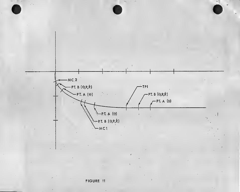
FIGURE II
5
of trajectory estimation errors, it is -generally undesirable for Ah
to be smaller than some value. If an analysis of the likely tra-
jectory dispersions indicates this may happen, or that it may grow
unacceptably large, an maneuver may be inserted into the flight
plan to minimize these effects.
2.9.3 Backup, Charts
2.9. 3.1 TPI Backups
The method employed in computing a backup TPI solution is that
of differencing the actual conditions observed just prior to TPI from
the condition^ required at TPI to achieve rendezvous oTt of orbit travel
later. The observables required for this technique are range (p) and
range rate (r) at a fixed time before IPI and two measurements of.
relative elevation angle ( 6 ) at fixed times before TPI. The solution
obtained is resolved into a velocity component along the line-of-sight
(AVj_os) at TPI and a velocity component normal to the line-of-sight
(AV^or* TPI. -Figure II shows the measurement geometry.
The algorithms used to compute the velocity along the line-of-
sight and the velocity normal to the line-of-sight are
Av,o3=r^Mi-AyiosiN)n R^ ^B(N) J
.w _rAVNOR(N) A^(N)-A^1n3/1 -
1
where
^^(Nr^B(N) “ ^A(N)
and At is the time between points A and B. The subscripts A and B
indicate the time at which an observable was measured, A being at
a time earlier than B. The subscripts N indicate those quantities
which are referenced to the nominal trajectory.
This approach depends on the fact that the catchup rate (x)
of the active vehicle with respect to the passive vehicle is very
nearly constant for coelliptic orbits, and is given by

6
where oj is orbital angular rate and is the differential altitude
between the tvro vehicles (see the derivation in section 2 . 9 .^).
It can be shown in the following manner that range rate is a func-
tion of catchup rate and relative elevation-angle.
LettingR
and differentiating, we get
R=[xx4 zz]/r 3*1 “ 2
But,- under the assumption that we are coelliptic,z = 0 and x/RcsiCos0
so
R= X COSd 3.1 - 3
Similarly, one can show that ,6 is a function of elevation angle:
0 -[xz - zx]/R^ “ 3.1-4
But z=0,5
z~Zo so
= --|ajsin2((9) 3.1 - 5
Hence, the values of 6, R, and 0 at B can be used to infer A and 0
at TPI. These predicted values can thus be differenced from the
required values to get a TPI solution.
The backiip chart is graphical in nature and the data used to plot
it are computed using a digital routine which generates the orbital
parameters for a set of trajectories covering the region of expected
dispersions about the nominal trajectory. The outputs of the routine
are functions of0g (the subscript denoting
the required values of the variables). For each of the ©-g's under
consideration, coelliptic orbits are generated and advanced back
in time by the appropriate At to get 6^ and hence, A0. The trajectories
are then advanced to TPI and the transfer maneuver is computed (see
section 2.9.,4.3)j ^Vlqs and AVnor • Then
RA =[Rii+'iVLOs]/R|3.1 - 6a
and-B
.
At 3.1 - 6b
are computed and stored.

prepared by fprb/ops
G MISSION TERMINAL PHASE INITIATION
MISSION APOLLO 11, MAY 16, 1569
FIGURE ill
7
Graphically, the solution for AVlos is obtained by taking the
product of (Vr)req ^ ^ subtracted from
to get AVlos • Likewise, is subtracted from the actual
A0 and multiplied by Rg/At to get AV^jqr* Figure III presents the
TPI chart as flown on Apollo 11.
It should be noted here that the midcourse correction (MCC)
charts are equivalent to TPI charts with the following exceptions:
1. The active vehicle is assurued to be on a collision course
with respect to the passive vehicle rather than in a coelliptic or-
bit as in the nominal case.
2. The MCC burn is assumed to occur at the instant of the second
measurement point, rather than a fixed time later.
With the exception of the above assumptions, the MCC charts are
generated and used in exactly the same manner as the TPI chart. Later
work on this problem has resulted in a TPI table, utilizing R, R, 9,
and the interval (At) between the last measurement and TPI.
2 . 9 . 3.2 CSI Bacl^ps
Since the AV for CSI is not, (in general) even approximately
available as a function of the observables, it is necessary to adopt
a somewhat different approach than that of the last section. Of the
standard mathematical techniques for approximating an unknown function;
the simplest is the Taylor Series. For CSI, only the in-plane problem
is to be solved; therefore, four independent measurements will serve
to constrain the problem. The simplest possibility is an equation of
the form
3.2 - 1
i.e., an uncoupled power series in the observables . Should this
assumption fail, it may be necessary to look for higher order cross
terms in particular cases. For the situation where CSI occurs as
the result of a nominal ascent from the lunar surface, and similar
trajectories, this assumption works well.
To determine the constants a^, b^, c^, d^, a set of trajectories

8
spanning the envelope of expected dispersions is required, together
vith the AVc5 ,
for each case. In the solution of this prohlem, measure-
ment time is held fixed to remove it as a.variable, and the values
of the observables, R and/or R are read at each measurement point.
When these are substituted into 3.»2 -•!, a system of simultaneous
algebraic equations result
aV,
AV2 q,• •
q, q^-•
'I.•
1
.
.
K)
—
1
• • • . . . • •
d,
d2
This system is generally well over determined, and writing
^7 =QCby the usual theory (2.9- 6)
c =[q*oJq’av
is the least squares fit of C to the systm. Having determined these
constants, a table of partial sums is constructed where each entry is
the partial sum of a particular value of a qj for various values.
Such a table is presented in Figure IV. For this case, the measure-
ments are R at CSI -30^ -20^, -10^ and a range at -10^. As each
measurement is obtained, its corresponding factor is looked up in
the table and logged in the space provided. At the last observation,
these factors are summed to give the aV(;-5 ,
.
2 . 9 . 3 . 3 CDH Backups
Early work on the CDH problem by Flight Procedures Branch elicited
the property that range rate in a near-coelliptical orbit is closely
representable by a sinusoid of the form
R=Ro+ RmCOS(<^* + Aujt) 3.3-1
By appeal to the linearized' relative equation it can also be shown
that
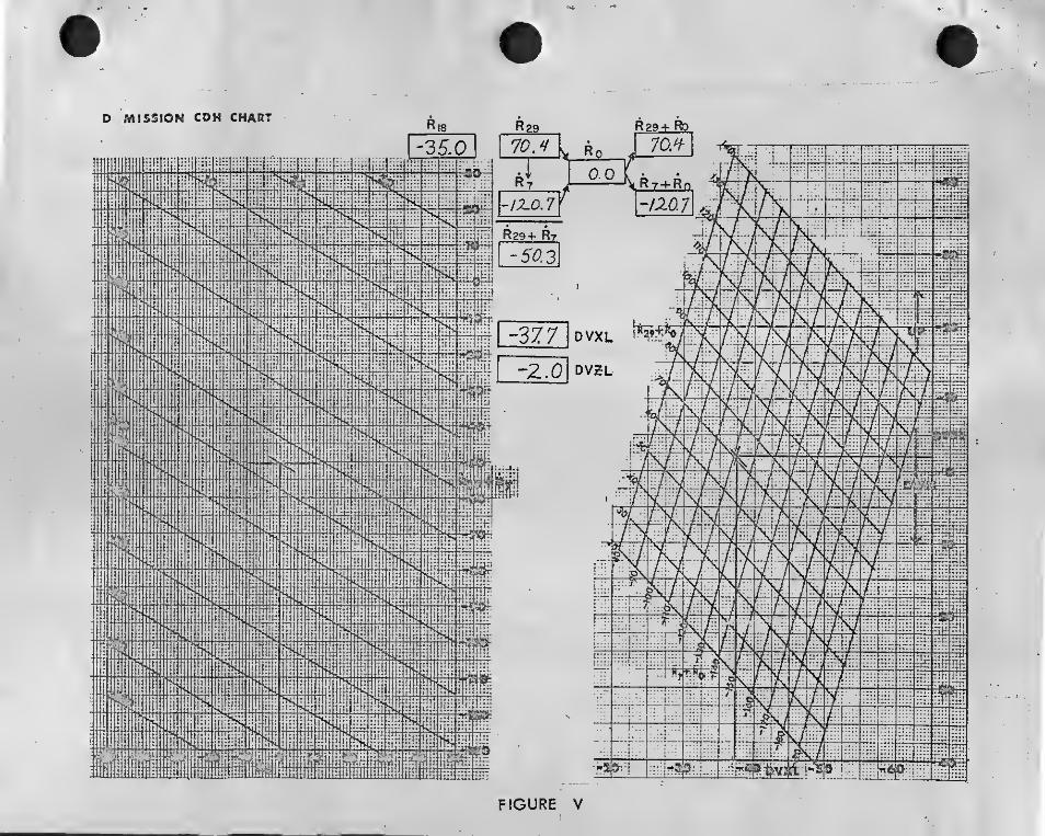
D MISSION CDH CHART
'2.0
'7-0 .
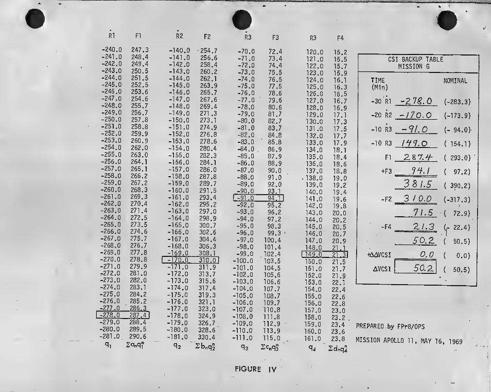
•240.0 247.3241.0 248.4242.0 249.4243.0 250.5244.0 251.5245.0 252.5246.0 253.6247.0 254.6248.0 255.7249.0 256.7250.0 257.8251.0 258.8
259.9
255.0 263.0256.0 264.1257.0 265.1
258.0 266.2259.0 267.2
268.3261.0 269.3262.0263.0 271.4264.0 272.5265.0 273.5
-266.
-267.
-268.
269.0270.0271.0272.0
-274.0
275.0276.0277.0278.0279.0280.0281.0
2
5.
276.
277.8278.8279.9281.0282.
283.1
284.2285.2
' 286.3
287.4288.4289.5
290.6
SOnq?'
0
0
0
.0
-175.0-176.0
177.0178.0179.0180.0181.0
^2
254.7256.6258.4260.2262.1
263.9265.7
267.6269.4271.3273.1
274.9
276.8278.6
280.4
282.3284.1
286.0287.8289.7
291.5
293.4
295.2
297.0
298.9
100.7
102.6
104.4
106.3
0
311.9313.7315.6317.4319.3321.1
323.0324.9326.7328.6'
330.4
2bnq2
92-93
-94
-95
-96
-97
-98-99
100
101
102
103
104.0105.0106.0107.0108.0109.0
110.0111.0
95.296.297.298.399.300.401.402.403.504.505.606.6107.7108.7109.7
110.8111.8112.9113.9115.0
2Cnq5
50
51
52
53
154.0155.0156.0
157.0158.0159.0
160.0
161.0
CSI BACKUP TABLEMISSION G
TIME NOMINAL(Min)
-30 R1 _ -m.o (-283.3)
-20 R2 _ -170.0 (-173,9)
-10 R3 _ -91.0 (- 94.0)
-10 R3 _ iHl.o ( 154.1)
FI _ as 7.^ ( 293.0)
+F3 _ 7^./ ( 97.2)
3 81.5( 390.2)
-F2^ 3 10.0 (-317.3)
71.5 ( 72.9)
-F4 _ a/.
3
(|- 22.4)
so.z { 50.5)
tAAVCSI 0.0( 0.0)
AVCSI [ 50.2.( 50.5)
^4 2dnq5
PREPARED. by FPrB/OPS
MISSION APOLLO 11. MAY 16. 1969
FIGURE IV
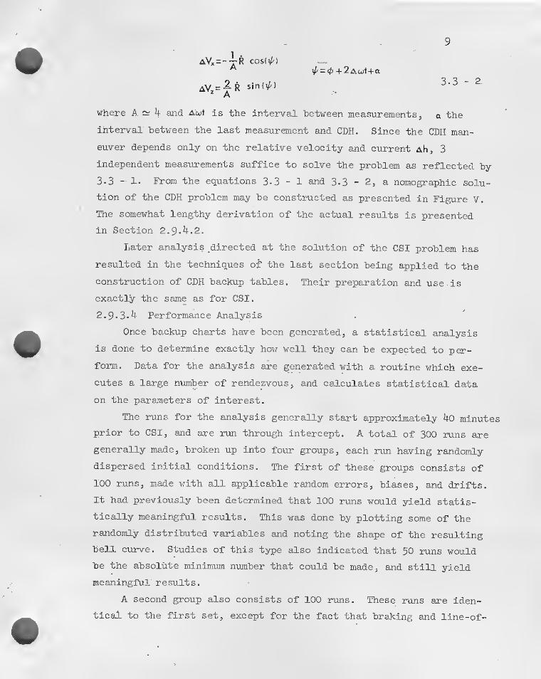
9
AVx =“-7R C0S{4')^ ^ = 4)+2Awt+a
aY,= -|- R sinf'/')^
A
where A ci? 4 and Awi is the interval between measurements, a the
interval' between the last measurement and CDH. Since the CDH man-
euver depends only on the relative velocity and current Ah, 3
independent measurements suffice to solve the problem as reflected by
3-3 - !• From the equations 3.3-1 and 3-3 - 2, a nomographic solu-
tion of the CDH problem may be constructed as presented in Figure V.
The somewhat lengthy derivation of the actual results is presented
in Section 2. 9.4.2.
Later analysis directed at the solution of the CSI problem has
resulted in the techniques of the last section being applied to the
construction of CDH backup tables. Their preparation and use -is
exactly the same as for CSI.
2. 9* 3. 4 Performance Analysis
Once backup charts have been generated, a statistical analysis
is done to determine exactly hovr well they can be expected to per-
form. Data for the analysis are generated with a routine which exe-
cutes a large number of rendezvous, and calculates statistical data
on the parameters of interest.
The runs for the analysis generally start approximately 4o minutes
prior to CSI, and are run through intercept. A total of 300 runs are
generally made, broken up into four groups, each run having randomly
dispersed initial conditions. The first of these groups consists of
100 runs, made with all applicable random errors, biases, and drifts.
It had previously been determined that 100 runs would yield statis-
tically meaningful results. This was done by plotting some of the
randomly distributed variables and noting the shape of the resulting
bell curve. Studies of this type also indicated that 50 runs would
be the absolute minimum number that could be made, and still yield
meaningful results.
A second group also consists of 100 runs. These runs are iden-
tical to the first set, except for the fact that braking and line-of-

Differences Between. Ch£.rt Solutions With and
Without Errors and Conic Solutions
Maneuver AverageSet Dft/sec
Set Aft/ sec
*CSI AAVj^ 0.0 .77
CDH AAV^ 1.11 1.54
CDH AAv„n
.25 .46
TPI 1.3^ 2.40
TPI- iAVjj *37 2.4i
MCCl 1.59 2.65
Mqpi AAVjj 1.34 2.16
;mcc2 .84 1.48
MCC2 AAVjj .50 1.29
MeanSet Dft/ sec
Set Aft/sec
Standard DeviationSet D Set Aft/sec ft/sec
0.0 - .02 0.0 .95
l.ll 1.05 1.21,
1.83
- .25 - *33 .34 .60
-i.o4 - .76 1.45, 3.02
- .29 - .44 .54 3.12
-1.59j
-1.83 .91 2.8Q^
1.34 1.4? .37 ' 2.26
- .82 - .97 59 1.48
.50 .85 .16 1.77
The data in Table 3-3 listed under Set D represents the theoretical error inherent in the charts,
while the data listed under Set A represents the total expected error, including theoretical error, system
errors, and execution errors.
*The value for CSI AAV represents the difference between CSI AV computed with sensor and reading errors,
and the value for CSI AV computed without sensor and reading errors.
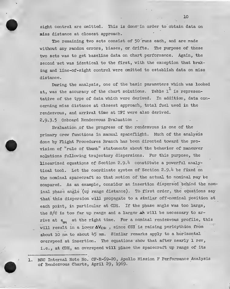
10
sight control are omitted. This is done-;in order to obtain data on
miss distance at closest approach.
The remaining two sets consist of 50 'runs each, and are made
without any random errors, biases, or drifts. The purpose of these
two sets was to get baseline data on chart performance. Again, the
second -set was identical to the first, with the exception that brac-
ing and line-of~sight control were omitted to establish data on miss
distance.
During the analysis, one of the basic parameters which was looked
at, was the accuracy of the chart solutions. Table 1 is represen-
tative of the type of data which were derived. In addition, data con-
cerning miss distance at closest approach, total fuel used in the
rendezvous, and arrival time at TPI were also derived.
2.9 . 3.
5
Onboard Rendezvous Evaluation .
Evaluation _of the progress of the rendezvous is one of the
primary crew functions in manual spaceflight. Much of the analysis
done by Flight Procedures Branch has been directed toward the pro-
vision of "rule of thumb" statements about the behavior of maneuver
solutions following trajectory dispersions. For this purpose, the
linearized equations of Section 2.9.4 constitute a powerful analy-
tical tool. Let the coordinate system of Section 2.9.4 be fixed on
the nominal spacecraft so that motion of the actual to nominal may be
compared. As an example, consider an insertion dispersed behind the nom^
Inal phase angle (up range distance). To first order, the equations say
that this dispersion will prop^ate to a similar off-nominal position at
each point, in particular at CDH. If the phase angle was too large,
the S/c is too far up range and a larger Ah will be necessary to ar-
rive at Tj at the right time. For a nominal rendezvous profile, this
will result in a lower AVcsi 5 since CSI is raising pericythion from
about 10 nm to about 45 nm. Similar remarks apply to a horizontal
overspeed at insertion. The equations - show that after nearly 1 rev,
i.e., at CDH, an overspeed will place the spacecraft up range of its
1. MSC Internal Note No. CF-R-69-20, Apollo Mission F Performance Analysis
of Rendezvous Charts, April 29, 1969*
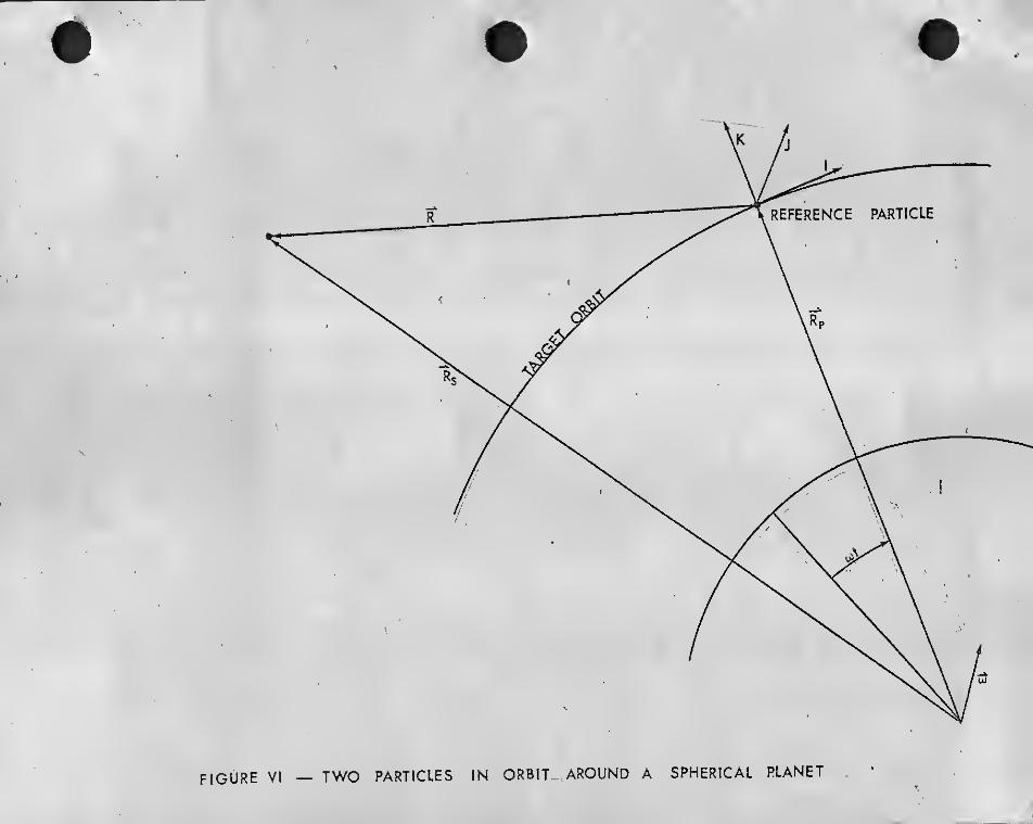
figure VI — TWO PARTICLES IN ORBIT. AROUND A SPHERICAL PLANET
11
nominal position. Converse statements apply to too small an insertion
phase angle or an insertion underspeed. If the insertion error is in
altitude rate, the actual spacecraft after one rev is nearly coinci-
dental with the nominal one, hut has an altitude rate error nearly
equal to that at insertion. Thus the vertical component of the CDH
maneuver will he perturbed to remove it, hut the resulting Ah will he
little affected. Provided the pilot has information on the disper-
sions resulting from a particular case, he can infer the trend of
his maneuver solutions in comparison to nominal.
By similar means, the effect of an incorrect CSI maneuver in
arrival time at may he gauged. Since CSI is strictly horizontal,
one need only consider dispersions in this axis and it is instantly
apparent that an overturn causes late arrival and conversely. For
lunar orhlt, this is about 4 min/fps.
2 . 9.4 Mathematical -and Technical Appendix
2. 9 . 4.1 The Linearized Relative Equations
All rendezvous problems have in common two basic requirements;
( 1 ) knovrledge of the relative motion between the interceptor and target,
and ( 2 ) a plan of maneuvers for the interceptor which results in a
terminal condition of zero relative velocity at a small distance.
In order to facilitate analysis and understanding of the rendez-
vous problem, it is useful to develop a set of equations describing
the relative motion of one vehicle with respect to another when they
are reasonably close. This follovrs the standard treatment, and two
assumptions will be adherred to in- the discussion:
1. The orbit of the r.eference particle is near circular.
2. The distance between them is small compared to the radius vec-
tor of the reference particle.
In Fig. IV, construct a coordinate system fixed on the reference
particle; , J = K |KxVp| ,1'"Jxl5 and defining
1 0 0— 0 1 0 a = 0 -COx
0 0 1 10K3>-3
_!_i

12
and noting and Rp constant by assumption 1.
,
operator for such a vector is
dAdt
d t2“ P at2 + 2 + n^] A
the derivative
Using these equations and writing with respect to Rp find Newton’s
Law for particle $
at24,1 - 2
i X
|y1
' z
+ 2 It} 0
-x
_u^2 0
z+Rp4.1 3
Now examine
if terms of second order are. ignored by assumption 2. This is the
first of two approximations to be made in the interest of obtaining
a linear system. Careful note should be taken of the implied limita-
tions on "^he result. The second approximation is gotten by assuming
terms of the form
3xz,
3yz,
3z2Rp Rp Rp
are also negligble, thus to get
ii 2'^ — to an<3^ writefarther identify
T
Relative Motion of Particle B; \
3Shape is characterized by ratio
of R — /'^moK
3 . Schneider, A.M. Report SDC-l-69
FIGURE VII

13
L J
it can be shown that because of the linearity of the equations, the
state at any time due for a combination of initial perturbations is
the same as the sum of the states at that time due to the perturbations
applied separately, i.e.:
^ B .e/o
” j^A B^oj A-e^o'*' B -^oj
--

l4
It may “be guessed from intuition and stated from experience that the
requirement that the reference particle orhit he circular may he relaxed
somewhat, provided that x is interpreted as down-range curvilinear
distance along the orhit arc, and z as normal distance from the point
X to the particle R^. . It should he stressed that even in regions where
the assumptions leading to linearity are not strictly true, the equa-
tions still provide a useful indication of the relative motion to he
expected.
2 . 9 . 4 . 2 CDH Equations
It is desired to relate the velocity maneuvers at CDH to the oh-
servahle, range rate. This will he measured at selected times before
GDH.
From Equation 3«1 - 2' of Section 3*2
R=[xx + zz}/H = XCOS7? z sin>?
Since at large ranges cost? and sin^? 0,
R - k 4.2-1
Equations 4.1 - 8a, hy defining
b ~2 C2 Zq 4- Xoj^ijJ
c= [2z:o/co-Xo]
p^-[(Zo/wf-(2(Xo/aj)+3Zo)^]
can he written7 = tan ’[zc/(2xo+3wZo}T
X =c+|b</? -2p sih(v547 )
z = b-pcost*^ +7 )
<p -= -wt
Therefore,
x= |b<4''2p'4cos(<^+7 }
i = p<p sm(<P47 )
For coellipticity, it is required
X=|wZo
z= 0
So that the components of CDH at any point are
A'sC= Xp^ x^= |;<pz
b
+ 2p<p cos (^+7 )
_|;(pb~|-''PPCOs[<p47)-|b^+2pV5cos(<P+Y)
c:^(^pCOS(<p+7 )
4.2 - 2
4.2 - 3
FIGURE VIII RENDEZVOUS PROBLEM
15
AVz = = - p sin (<P+7
)
Taking the first equation of 4.2 - 2 and defining
Rc“|bv3
Rm=-2p(phave
R = R^+R^sinitp+T)
4.2. - 4
as the equation .to be solved. Taking t=0 at the first measurement
noting that three will be required to determine R^. > 7 :
Ro= Rc + RmSrn( y )
R, = Rc’*'Rmsin(«p+7)
^=Rc + R^sin(2<p+Y)
After considerable manipulation, the solution of this simultaneous set
can be obtained as . . .• - •
'
sm7=(Ro- Rc)/Rm
R= [Ro+ R2”2RjCOS “cosv^j Rg^= Ro “ Rc
R=pEo'^RE2“2RE2RE„COS2<p]/iin2<p ^£3= R2 " Rc
Therefore, if a is the elapsed central angle between the last measure-
ment and the time of CDH, the maneuvers are given by
-^R^cos{2'P + 7+a)
AV,= 4RrnSin(2‘P+7+ a)
2. 9 . 4.3 Digital Computation of Transfer
In general, a transfer problem consists of. finding the
velocity maneuver required to go between given points subject
to various constraints.
It is desired to solve the time of flight problem, in a man-
ner appropriate for use with a digital computer.
As in figure VIII, let a Clohessy-Wiltshire (C-W) frame
be attached to the passive particle, with co., Xo, X©,
given.
Then from the last section
X(t) = A(tut)Xo+BG^./t)X. 4.3 - 1

l6
Where A(wt) ,B(c^t) are the C-VJ matrix functions of time. For
intercept require X(t) = 0 after a time t:
A(u)t)Xo+B(cx)t)Xr - 0 ' 4.3-2
Xr = -E-’ (tot)A(a)t)Xo
4.3 - 3
Since maneuvers -vn.!! be done in the active vehicle local
vertical frame, compute
Rs = (Rf +Xo )+ u x(Rt +Xo )
= RtRt-'-Xr+ wx(Rj+Xr )
'cos4>
sin0
-s±n<f
COS0Rs = Central angle at intercept.
in the local vertical frame of the active vehicle.
If this Xr is applied, and the active vehicle precisely
advanced along the resulting orbit, it will not, in general,
intercept the origin. This is due to the approximate nature
of the C-W equations, which results in an X^ residual at the
time for intercept. At this juncture, one may proceed in two
similar but slightly different ways, both of which will be
discussed.
1. Offset Targeting
Note that the general solution of the C-W equations
for Xr is
Xj = B"’ (wt)X(t)-B"’ (a;t)A(wt)Xo 4.3 - 4
In V7hich x(t) was set equal to zero for intercept.
Since the solution obtained is kno\m to miss by Xg^
retarget for -Xe and reasonably expect to hit in between
Xf and -Xe , i.e., near the origin:
±r = -B-’ (wt)Xe -B‘(wt)A(a;t)Xo 4.3 - 5
17
This may again miss hy X^say, and a "better solution
may be obtained as before Jby^. aiming for -Xc :
-B-’ (a.t)[Xf +X^ 1 -B-’ (a;t)AUt)Xo ^*3 - 6
and so on•
I
nr;}.
X"'=-B-’(ot) 2]x; -B-’-(ot)A(u.t)Xo‘=0-
4.3 _ 7
where Xe;= 0
one may consider this an iteration on initial displace-
ment by noting that the operation A(vrt) transforms an
initial displacement into a final displacement:
Xf = A(ajt)Xi-4 3 _ 8
thus targeting for is the" same as perturbing X© by
A“’ (wt)lil and leads to the equation
X; - -B"' (a-t)A(a;t)[Xo+A“’ ^ Xe ] 4^3 _ g
where A“’ may be considered a matrix gain factor determin-
ing how an intercept error should perturb the initial dis-
placement to effect convergence.
2 . Successive C-W Frames
Attach a C-¥ frame to the active particle and
imagine that at intercept, the passive vehicle has a
position -Xf in this frame. Then in this frame compute
a velocity maneuver which would send a particle to this
point from its origin in an (wt)' =-A>^s. Where A is the
change in the tzue anomaly of this new frame from transfer to
intercept:
Xf = (wt) Xf
Add this correction to the initial guess and proceed as
before
:
n-l
Xr = - (at)iXf -B-’ (wt)A(Lot)Xoi-O
18
in effect constituting a new C-W frame at Xt for each
attempt, computing a solution to_ drive a particle to. -Xe ,
and summing these.
Note that the propriety of these two methods lies in
the tendency of the C-¥ equations to give exact results as
the distance between the particles approaches zero.
2.9.4. 5 CSl/CDH
Considering first the CDH maneuver, there are several
ways to rigorously define coellipticity. The one in use for
Apollo results in alignment of the semi-major axes and no
variation in Ah to first order. In terms of the eccentric
anomoly for each vehicle
R^=a^(l-e^ cos E^)
cos E^)
therefore
Ah=R2-R^=a2-a^+a^w^ cos ^2
=AhQ-f-(a^e^ cos ^^"^2^2 ^2^
In order for there to be no variation in Ah, it must be true
that (0 = phase angle) so that when the vehicle
radius vectors are coincident E^-E^:
^CDH
Then if a^e^=a2e2 5 h will be constant. It can be shown that
for given true anomoly of both vehicles the same, the variation2 2
in Ah is the order of
For CSI, a straight iterative procedure is 'used wherein
a trial velocity for a CSI is varied to compute a numerical
partial derivative of change in with respect to change
in AVc5, ,
2. 9.4.6 Multiple Linear Regression
Let an over-determined system of equations be given
RC = aV+ €
19
where Risahmxn m>n known matrix and 'C is an n-row hy
l-colunin. Since the system is overdetermined, t will not
in general hy zero, hence let us seek to minimize its magnitude:
< = RC-^V ^.6 - 2
*2= P e'= (c*R’~ aV’)(RC - aV) 4.6 - 3a
= C'r^RC -(C'R^aV +aV^RC) +aVaV 4.6 - 3h
/ai extremxim (hopefully minimum) of p will he found when
the variation consequent upon a variation 6C is zero,
i.e. require:
j,2=2[5C'r'RC-«c'r'aV] = 0 4_g . 4
since 6aV= 5R=0. Novf note that if a , a scalar is
a = K'K=(K'K)=a^
Since is a scalar conclude that each term of h.6 - 4
is scalar and substitute for .C*R^R6C and aV'R5C
their transposes.
Since the variations 6C are arbitrary, we conclude that
is minimum if ^r'rc-r'av=o
C = (R*RrVAV‘ 5
2 . 9 . 4 .? Digital Programs
Several digital programs have been developed for use in
the generation and verification of backup charts and the
study of the rendezvous problem. One of these, used for all
of the above purposes, is a large multi-purpose Fortran pro-
gram called Betelgeuse. It has the capability to integrate
two vehicles through either Earth or. Lunar orbit.
.The program utilizes standardized input and output rou-
tines. As a normal course of events, approximately 40 different
parameters arc output at each integration step.
A set of subroutines are available which are designed to
solve for each of the maneuvers required in the Concentric
20
Flight Plan. Included in these is the capability to execute
externally supplied aV maneuvers. Taken together, these
features provide a flexible tool for the study of rendezvous.
Additionally, the program has the capability to generate up
to 100 consecutive Monte Carlo runs, each with randomly dis-
persed initial conditions. This feature is used to make the
runs which yield data for the construction of backup charts.
Another set of subroutines in the program represent a
mechanization of the backup charts. These routines are capable
of sampling data during a run, calculating, and applying the
required maneuvers. In addition, there is a routine which
executes braking and line-of-sight control during the final
phase of the rendezvous. Random errors, biases, and drifts
are included in each of these Subroutines to make the simula-
tion realistic. These routines are used in conjunction with
the above _jnentioned Monte Carlo generator and a set of statis-
tical analysis routines for performance analyses of backup
charts
.
A second Fortran program is used to generate the coef-
ficients needed for CSI and CDH backup charts, which are
based on Maclaurin expansions. The program takes data derived
from Betelgeuse runs, and processes it using a multiple linear
regression technique, yielding the required coefficients.
A third Fortran program is used to generate data for TPI
and mid-course backup charts. It' has all of the required
equations mechanized, and outputs data which can be directly
plotted to yield a backup chart
.