Embed Size (px)
Citation preview
CoWWAn: Model-based assessment of COVID-19epidemic dynamics by wastewater analysis
Daniele Proverbio1, Francoise Kemp1, Stefano Magni1, Leslie Ogorzaly2,Henry-Michel Cauchie2, Jorge Goncalves1,3, Alexander Skupin⇤1,4,5, and Atte Aalto*1
1University of Luxembourg, Luxembourg Centre for Systems Biomedicine, 6 av. du Swing, Belvaux, 4376,Luxembourg
2Luxembourg Institute of Science and Technology, Environmental Research and Innovation Department, Belvaux,4422, Luxembourg
3University of Cambridge, Department of Plant Sciences, Downing St, Cambridge CB2 3EA, UK4University of Luxembourg, Department of Physics and Materials Science, 162a av. de la Faıencerie, Luxembourg,
1511, Luxembourg5University of California San Diego, 9500 Gilman Dr, La Jolla, CA 92093, USA
Abstract: We present COVID-19 Wastewater Analyser (CoWWAn) to reconstruct the epidemic dy-
namics from SARS-CoV-2 viral load in wastewater. As demonstrated for various regions and sam-
pling protocols, this mechanistic model-based approach quantifies the case numbers, provides epi-
demic indicators and accurately infers future epidemic trends. In situations of reduced testing capac-
ity, analysing wastewater data with CoWWAn is a robust and cost-effective alternative for real-time
surveillance of local COVID-19 dynamics.
Effective mitigation of the COVID-19 epidemics relies on reliable estimates of the epidemic dynam-ics. Analysing SARS-CoV-2 abundance in wastewater offers a cost-effective alternative to population-based large scale testing [1, 2] and is largely independent of healthcare-seeking behaviors, access toclinical testing and asymptomatic cases [3]. It thus bears the potential for faster and more reliable earlywarning indications for long-term epidemic surveillance [4, 5, 6]. To date, more than 50 countries and260 universities have wastewater surveillance systems in place [7]. However, despite improved exper-imental procedures and data processing [8], most of the current analysis approaches are restricted toqualitative and semi-quantitative retrospective studies of lagged correlations [9, 10]. These have lim-itations in quantitatively inferring the shedding population or in providing reliable projections of theepidemic dynamics. To address this challenge and fully exploit the potential of SARS-CoV-2 wastewa-ter abundance measurements, we developed CoWWAn as an automated approach that causally infersthe shedding population, estimates the effective reproduction number Reff, and provides projectionsof future epidemic trends. Quantifying these variables allows assessing the epidemic status within aregion and comparing it between regions, and supports effective mitigation policy making.
CoWWAn couples a mechanistic epidemiological model, describing the infection dynamics througha Susceptible-Exposed-Infectious-Removed (SEIR) process [11], with an Extended Kalman filter (EKF)[12] (Fig. 1a) for robust integration of noisy measurement data into a predictive modelling framework(Methods). The underlying SEIR model allows interpreting the inferred infection dynamics in termsof transmitting interactions, overcomes the interpretability and extrapolation limitations of correlation-based statistical approaches [13, 14] and, once calibrated, provides reliable estimates of the sheddingpopulation and future development of the epidemic. To demonstrate its general applicability, we ap-plied CoWWAn to public datasets from 12 regional areas from Europe and North America (Supplemen-tary Tab. 1), associated with different population sizes and based on different wastewater data process-ing protocols. Details on datasets, list of considered regions and selection criteria are given in Methodsand Supplementary Tab. 1, Supplementary Figs. 1 and 2.
*Corresponding authors: [email protected] and [email protected]
1
After appropriate calibration to test cases, CoWWAn quantitatively reconstructs the time evolutionof observed cases from wastewater data (Fig. 1b) by inferring the internal variables and parametersof the SEIR model. These include the susceptible, exposed and infectious population fractions, dailydetected cases and time-dependent infection rate (Methods). In our case studies, full time series datawere used for calibration for each region. When clear regime shifts in testing/sampling protocols areobserved, the model can be re-calibrated appropriately to improve the performance, like for Kitchener(Methods and Supplementary Tab. 2). To infer the global shedding population, the model needs addi-tional information on the ratio of total and detected cases, typically obtained from prevalence studies(Methods). A comparison with linear regression (after data curation to reduce the noise) reveals thatCoWWAn’s inferences achieve consistently higher correlation (Fig. 1d, blue and red sets), demonstrat-ing the power of our mechanistic-based approach. These observations hold for all considered regions(Fig. 1c and Supplementary Fig. 3-14): the correlation coefficient ⇢ between inferred case numbers andtrue detected case numbers is typically in the range between 0.7 and 0.9 even for rather noisy data likeNetherlands. Frequent sampling improves the model calibration and the subsequent reconstruction per-formance, like for Luxembourg with ⇢ = 0.91 for two probes/week and Milwaukee with ⇢ = 0.95 fortwo (sometimes more) probes/week compared e.g. to Barcelona with ⇢ = 0.70 with one probe/week(Fig. 1d). The main discrepancies originate from either unnoticed changes in the share of detected casesor from changes in testing/sampling strategies (Supplementary Fig. 3-14). Detecting such discrepan-cies can provide additional evidence about potential undertesting and could guide targeted scaling ofpopulation tests. Interpolating wastewater data points before the EKF estimation can improve the re-construction (Fig. 1d, red and yellow sets), in particular for regions with low sampling frequency likefor Barcelona Prat de Llobregat (PdL) and Kranj. In general, the Extended Kalman filter improves itspredictions as new data points are available, so an adequate sampling rate is recommended to improveits performance.
In addition, CoWWAn estimates the effective reproduction number Reff, an essential indicator for thetrends of epidemic diffusion in a community [15], which depends on containment measures, infectivityof viral variants, population behavior and other factors. As exemplified for Luxembourg (Fig. 1b), theReff values inferred by CoWWAn from wastewater data are consistent with the indicator reported by theMinistry of Health on its website (Methods) and exhibit the same noteworthy trends: the three wavesin 2020 (March, June and late October), a small rebound in March 2021 and one wave in late June 2021,all characterised by Reff > 1. For all other considered regions as well, wastewater-based Reff values areconsistent with those estimated from case numbers (Supplementary Fig. 3-14) and are usually smootherdue to sampling frequency and independence to testing schemes.
CoWWAn’s underlying SEIR model permits mechanistic-based projections of the infection dynam-ics, for effective monitoring of the epidemic. To produce projections of future trends, it is possible tostop the reconstruction at any desired time and simulate the model forward, starting from the lateststate estimate and keeping the transmission parameter constant (Methods). For the epidemic dynam-ics in Luxembourg, Fig. 2a shows an example of such 7-days projections for each day of wastewatersampling, where the number of detected cases (blue) is compared with the projected numbers derivedfrom wastewater data or from case number data. Wastewater-based projections are well correlated bothwith case-based projections (⇢ = 0.95) and with true case numbers (⇢ = 0.94). Overall, for the differ-ent epidemic phases and all considered regions, the projections compare well with the real case dataand with the case-based projections (Supplementary Fig. 3-14). To quantify the projection performance,we determined the average standardised projection error as the average discrepancy between projectedand actual case numbers in the corresponding time frame, normalised to case numbers and equivalentpopulation (Methods Eq. 10). The performance of our wastewater-based pipelines is usually slightlylower, as they reconstruct the case numbers themselves before making the projections, but remains sim-ilar with that of case-based projections: all regional estimates lie within one standard deviation of the1:1 (equal performance) line (Fig. 2b). The only exceptions are projections for Oshkosh, probably dueto under-testing during late 2020 (Supplementary Fig. 2) which induced discrepancies in the detectedcases fraction, and Kranj, whose low case numbers are subject to larger uncertainties (SupplementaryFig. 5). In general, the largest discrepancies are observed when case numbers plateau or decline after arapid increase, yielding a potential overshoot of the projections (Fig. 1a and Supplementary Fig 3-14).This effect is associated to large changes in social activities during epidemic waves and rapid imple-mentations of stricter restrictions, which are not explicitly included in the model but implicitly learned
2
from the epidemic curve by the EKF with some delay.The standardised error grows quite linearly with increasingly long projection horizons (Fig. 2c),
where wastewater projections are more stable (their uncertainty grows slower for longer projectionhorizons) than those based on case numbers as they are usually less susceptible to daily fluctuations(Supplementary Tab. 2). Due to heterogeneous and evolving adaptations of population behavior andinstitutional measures, epidemic forecasts are typically only meaningful for relatively short time hori-zons [16]. In particular for the real-time detection of impending epidemic resurgence, distinguishing be-tween fluctuations and robust increases is crucial to optimise the true positive signals and minimise thefalse negatives. CoWWAn addresses this challenge by the EKF-based projections, which capture robusttrends in the epidemic dynamics and allow for early warning of COVID-19 resurgence from case-basedand wastewater-based projections (Fig. 2d and Supplementary Fig. 16). On the other hand, long-termprojections that assume no changes in infection dynamics can be useful for counterfactual analysis ofcurrent measures (Supplementary Fig. 15). This analysis demonstrates the potential of wastewater datato inform investigations of incoming trends and quantifies the precision of this cost-effective surveil-lance method. Finally, CoWWAn’s EKF-based approach enables integrating different types of data tofurther improve the quality of projections. Including both wastewater and case data slightly but sys-tematically improves the projection accuracy compared to case data alone (Fig. 2c and SupplementaryTab. 2), suggesting that wastewater data contains independent information about the state of the epi-demics [17].
In summary, leveraging wastewater data with CoWWAn as an automated and mechanistic approachallows for new avenues for epidemic monitoring. In situations of reduced population testing, CoWWAncan support the reconstruction of the infection curves from wastewater data and allows projections offuture trends, in particular close to epidemic resurgence. Hence, it can trigger community-wide alertsto elicit targeted studies. Since hospital admission is typically downstream of the susceptible-exposed-infectious flow [18], an early detection of positive increases, supported by quantitative models thataccount for noise, could provide crucial information for healthcare management [19, 20]. The flexibilityof our freely available approach, its ease of implementation and its performance make it an importanttool for long-term monitoring and support of epidemic mitigation.
Author contributions
D.P. and A.A. conceptualised the project. L.O. and H.M.C generated the data for Luxembourg. D.P., F.K.,L.O., A.S. and A.A. analysed the data. D.P., A.A. and F.K. designed and developed the model. D.P. andA.A. implemented the code. All authors analysed and interpreted the results. J.G. and A.S. supervisedthe project. L.O., H.M.C. J.G. and A.S. acquired the funding. D.P. and A.A. wrote the first draft. Allauthors contributed to and approved the final manuscript.
Acknowledgments
The authors want to thank the Research Luxembourg COVID-19 Task Force for general support andcollaborative spirit. D.P. and S.M. are supported by the Luxembourg National Research Fund (FNR)through PRIDE15/10907093/CriTiCS and F.K. by the FNR project PRIDE17/12244779/PARK-QC. A.A.is supported by the FNR through CORE19/13684479/DynCell. L.O. and H.M.C. are supported by theFNR through the COVID-19-FT2/14806023 /Coronastep+. J.G. is partly supported by the 111 Project onComputational Intelligence and Intelligent Control, ref B18024.
Competing interests
The authors declare no competing interests.
Data availability
The wastewater and case numbers data that support the findings of this study are available from thewebsites listed in Methods (Data) and Supplementary Tab. 1. Luxembourg data for this study are avail-able at gitlab.lcsb.uni.lu/SCG/cowwan.
3
Code availability
CoWWAn’s implementation for Matlab 2019b is available at gitlab.lcsb.uni.lu/SCG/cowwan.
References
[1] Farkas, K., Hillary, L. S., Malham, S. K., McDonald, J. E. & Jones, D. L. Wastewater and publichealth: the potential of wastewater surveillance for monitoring COVID-19. Curr. Opin. Envir. Sci.Heal. 17, 14–20 (2020).
[2] Larsen, D. A. & Wigginton, K. R. Tracking COVID-19 with wastewater. Nat. Biotechnol. 38, 1151–1153 (2020).
[3] Peccia, J. et al. Measurement of SARS-CoV-2 RNA in wastewater tracks community infection dy-namics. Nat. Biotechnol. 38, 1164–1167 (2020).
[4] Weidhaas, J. et al. Correlation of SARS-CoV-2 RNA in wastewater with COVID-19 disease burdenin sewersheds. Sci. Total Environ. 775, 145790 (2021).
[5] Wurtzer, S. et al. Evaluation of lockdown effect on SARS-CoV-2 dynamics through viral genomequantification in waste water, Greater Paris, France, 5 March to 23 April 2020. Eurosurveillance 25,2000776 (2020).
[6] Randazzo, W., Cuevas-Ferrando, E., Sanjuan, R., Domingo-Calap, P. & Sanchez, G. Metropolitanwastewater analysis for COVID-19 epidemiological surveillance. Int. J. Hyg. Envir. Heal. 230, 113621(2020).
[7] Naughton, C. C. et al. Show us the data: Global covid-19 wastewater monitoring efforts, equity,and gaps. medRxiv (2021).
[8] Daughton, C. G. Wastewater surveillance for population-wide COVID-19: the present and future.Sci. Total Environ. 736, 139631 (2020).
[9] Nemudryi, A. et al. Temporal detection and phylogenetic assessment of SARS-CoV-2 in municipalwastewater. Cell Rep. Med. 1, 100098 (2020).
[10] Zhu, Y. et al. Early warning of COVID-19 via wastewater-based epidemiology: potential and bot-tlenecks. Sci. Total Environ. 145124 (2021).
[11] Anderson, R. M. & May, R. M. Population biology of infectious diseases: Part I. Nature 280, 361–367(1979).
[12] Kalman, R. A new approach to linear filtering and prediction problems. J. Basic Eng. 82, 35–45(1960).
[13] Li, X. et al. Data-driven estimation of COVID-19 community prevalence through wastewater-basedepidemiology. Sci. Total Environ. 147947 (2021).
[14] Cao, Y. & Francis, R. On forecasting the community-level COVID-19 cases from the concentrationof SARS-CoV-2 in wastewater. Sci. Total Environ. 786, 147451 (2021).
[15] Huisman, J. S. et al. Wastewater-based estimation of the effective reproductive number of sars-cov-2. medRxiv (2021).
[16] Petropoulos, F. & Makridakis, S. Forecasting the novel coronavirus covid-19. PloS one 15, e0231236(2020).
[17] Fernandez-Cassi, X. et al. Wastewater monitoring outperforms case numbers as a tool to trackcovid-19 incidence dynamics when test positivity rates are high. Water research 200, 117252 (2021).
4

[18] Kemp, F. et al. Modelling COVID-19 dynamics and potential for herd immunity by vaccination inAustria, Luxembourg and Sweden. J. Theo. Biol. 110874 (2021).
[19] D’Aoust, P. M. et al. Catching a resurgence: Increase in SARS-CoV-2 viral RNA identified inwastewater 48 h before COVID-19 clinical tests and 96 h before hospitalizations. Sci. Total Envi-ron. 770, 145319 (2021).
[20] Saguti, F. et al. Surveillance of wastewater revealed peaks of SARS-CoV-2 preceding those of hos-pitalized patients with COVID-19. Water Res. 189, 116620 (2021).
5
a
Real system Model
Kalman gain
MeasuresModelledmeasures
+ −
01/03 01/05 01/07 01/09 01/11 01/01 01/03 01/05 01/07Date
0
100
200
300
400
500
600
700
Posi
tive
dete
cted
cas
es
0
0.5
1
1.5
2
2.5
3
3.5
4
4.5
SAR
S-C
oV-2
RN
A ab
unda
nce
in w
aste
wat
er
1012 S
E
I
R
A
yc
yw
β
α
τ∅
γ
b
c
Case numbers
Reco
nstru
cted
cas
e nu
mbe
rs
0 1320 26400
1000
2000
3000Barcelona PdL
0 50 1000
20
40
60
80
100Kitchener
0 70 1400
50
100
150Kranj
0 230 4500
100
200
300
400
500Lausanne
0 190 3800
100
200
300
400Ljubljana
0 450 8900
200
400
600
800
1000Luxembourg
0 350 7000
200
400
600
800
1000Milwaukee
0 6520 130400
5000
10000
15000Netherlands
0 50 1000
20
40
60
80
100Oshkosh
0 330 6600
200
400
600
800
1000Raleigh
0 30 500
10
20
30
40
50Riera de la Bisbal
0 250 5000
100
200
300
400
500Zurich
d
0
300
600
900
Daily
new
cas
es
Estimated from WW dataDataFrom Lux Health Ministry2SD envelope
01/03 01/05 01/07 01/09 01/11 01/01 01/03 01/05 01/07 Dates 2020-21
0.5
1
1.5
2
R eff
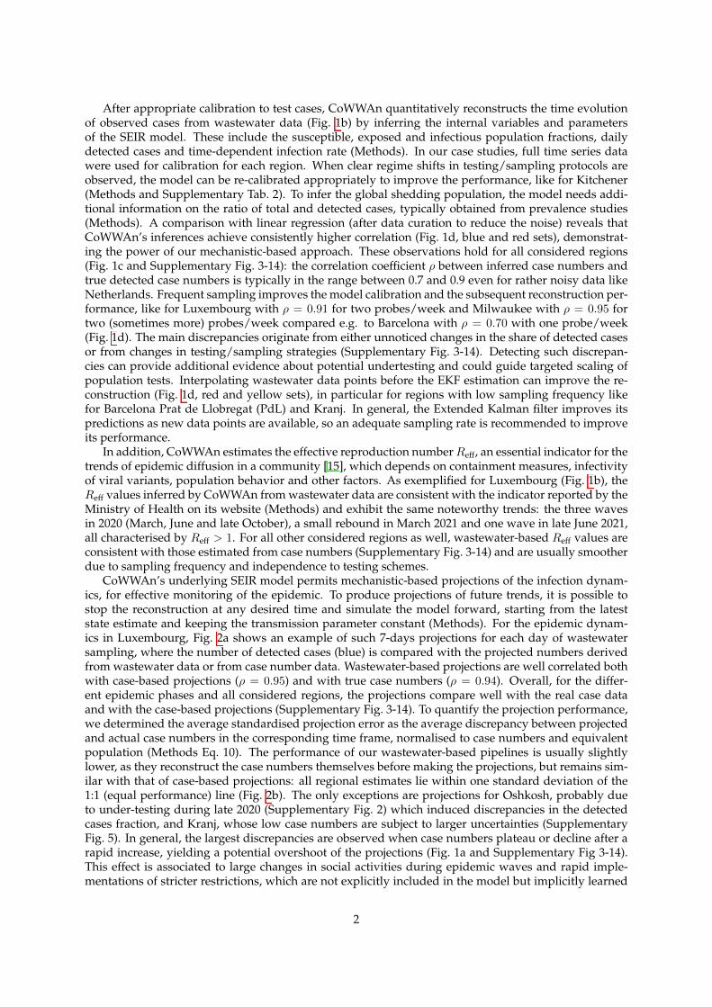
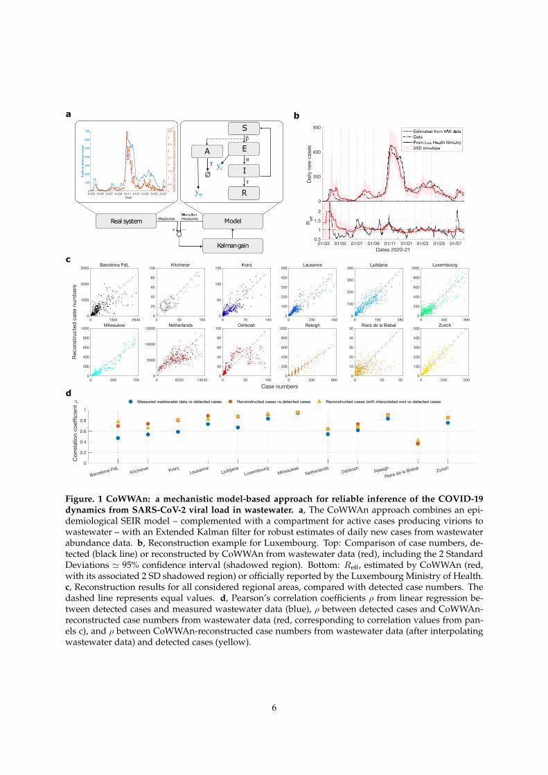
Figure. 1 CoWWAn: a mechanistic model-based approach for reliable inference of the COVID-19
dynamics from SARS-CoV-2 viral load in wastewater. a, The CoWWAn approach combines an epi-demiological SEIR model – complemented with a compartment for active cases producing virions towastewater – with an Extended Kalman filter for robust estimates of daily new cases from wastewaterabundance data. b, Reconstruction example for Luxembourg. Top: Comparison of case numbers, de-tected (black line) or reconstructed by CoWWAn from wastewater data (red), including the 2 StandardDeviations ' 95% confidence interval (shadowed region). Bottom: Reff, estimated by CoWWAn (red,with its associated 2 SD shadowed region) or officially reported by the Luxembourg Ministry of Health.c, Reconstruction results for all considered regional areas, compared with detected case numbers. Thedashed line represents equal values. d, Pearson’s correlation coefficients ⇢ from linear regression be-tween detected cases and measured wastewater data (blue), ⇢ between detected cases and CoWWAn-reconstructed case numbers from wastewater data (red, corresponding to correlation values from pan-els c), and ⇢ between CoWWAn-reconstructed case numbers from wastewater data (after interpolatingwastewater data) and detected cases (yellow).
6
a
d
c
0 2 4 6 8 10 12 14 16 18 20
Projection horizon (days)
0
2
4
6
8
10
12
Aver
age
stan
dard
ised
erro
r per
100
,000
inh.
WastewaterCasesCombined
01/03 01/05 01/07 01/09 01/11 01/01 01/03 01/05 01/07Dates 2020-21
0
1000
2000
3000
4000
5000
6000
7000
8000
Cas
es d
urin
g 7-
days
win
dow
Case numbers data)7d Projection (wastewater)7d Projection (cases)
0 2 4 6 8 10 12
Average standardised error per 100,000 inh.(7-days projections from case numbers)
0
5
10
15
20
25Av
erag
e st
anda
rdis
ed e
rror p
er 1
00,0
00 in
h.(7
-day
s pr
ojec
tions
from
was
tew
ater
dat
a)Barcelona PdLKitchenerKranjLausanneLjubljana
LuxembourgMilwaukeeNetherlandsOshkoshRaleigh
Riera de la BisbalZurich1:1
b
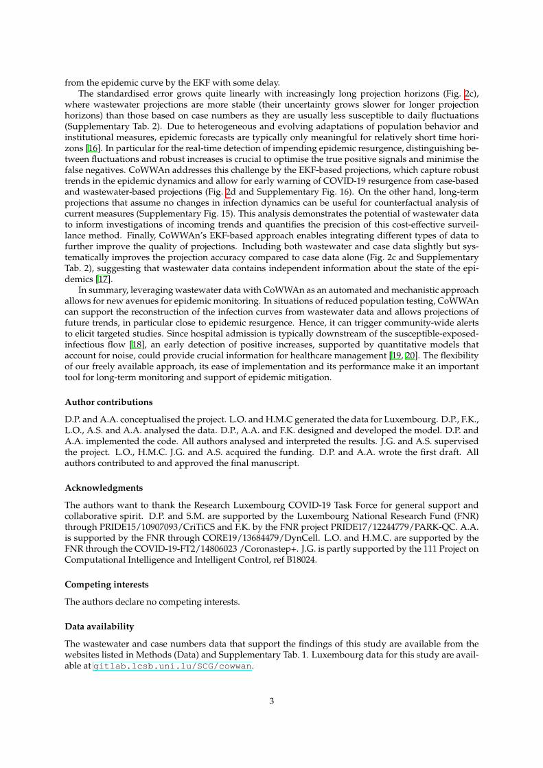
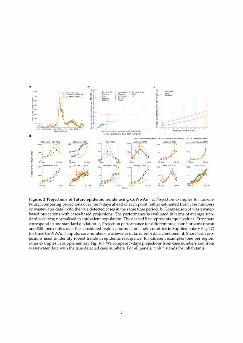
Figure. 2 Projections of future epidemic trends using CoWwAn. a, Projection examples for Luxem-bourg, comparing projections over the 7-days ahead of each point (either estimated from case numbersor wastewater data) with the true detected cases in the same time period. b, Comparison of wastewater-based projections with cases-based projections. The performance is evaluated in terms of average stan-dardised error, normalised to equivalent population. The dashed line represents equal values. Error barscorrespond to one standard deviation. c, Projection performance for different projection horizons (meanand 80th percentiles over the considered regions; outputs for single countries in Supplementary Fig. 17)for three CoWWAn’s inputs: case numbers, wastewater data, or both data combined. d, Short-term pro-jections used to identify robust trends in epidemic resurgence, for different examples (one per region;other examples in Supplementary Fig. 16). We compare 7-days projections from case numbers and fromwastewater data with the true detected case numbers. For all panels, “inh.” stands for inhabitants.
7
Methods:CoWWAn: Model-based assessment of COVID-19
epidemic dynamics by wastewater analysis
Daniele Proverbio1, Francoise Kemp1, Stefano Magni1, Leslie Ogorzaly2,Henry-Michel Cauchie2, Jorge Goncalves1,3, Alexander Skupin⇤1,4,5, and Atte Aalto*1
1University of Luxembourg, Luxembourg Centre for Systems Biomedicine, 6 av. du Swing, Belvaux, 4376, LU2Luxembourg Institute of Science and Technology, Environmental Research and Innovation Department, 4422
Belvaux, Luxembourg3University of Cambridge, Department of Plant Sciences, Downing St, Cambridge CB2 3EA, UK
4University of Luxembourg, Department of Physics and Materials Science, 162a av. de la Faıencerie, Luxembourg,1511, Luxembourg
5University of California San Diego, 9500 Gilman Dr, La Jolla, CA 92093, US
October 15, 2021
1 Methods
1.1 DataWastewater data and case numbers were obtained from different sources, listed in Supplementary Tab. 1along with the countries considered and their associated equivalent population (i.e., the ratio of thesum of the pollution load collected during 24 hours by sewage facilities and services to the individualpollution load in household sewage produced by one person in the same time. It is a proxy of thenumber of people who contributed to the wastewater load). Our pipeline was tested on datasets withdifferent normalisation protocols for wastewater data, to show its general applicability after propercalibration. We refer to each source for details about the experimental protocols. The units of measureof wastewater data, according to the official sources, are reported in Supplementary Tab. 1.
The selection criteria for data collection are the following. First, we employed the COVID19 PoopsDashboard [21] to list all worldwide resources about wastewater sampling projects; among those, wefocused on those having readily accessible databases. To allow proper calibration of the model, weselected time series data starting no later than beginning 2021, having at least one sample per weekon average and having the corresponding case numbers available. We rejected wastewater data withsmoothing among data points to avoid introducing bias and breaking the causality of projections. Fi-nally, if time series from multiple treatment plants were available from a single regional database, weselected the two representative ones, usually with the largest population.
The selected datasets, from specific wastewater treatment plants or covering bigger regional ar-eas, are the following: Barcelona Prat de Llobregat (Spain), Kitchener (Canada), Kranj (Slovenia), Lau-sanne (Switzerland), Ljubljana (Slovenia), Luxembourg, Milwaukee (USA), Netherlands, Oshkosh (US),Raleigh (US), Riera de la Bisbal (Spain), Zurich (Switzerland). Data from Luxembourg sewage samplingwere made available by the Research Luxembourg COVID-19 initiative CORONASTEP (researchluxembourg.lu/coronastep), while case numbers and Reff were obtained from the LuxembourgMinistry of Health website (COVID19.public.lu/fr/graph). Other datasets were downoaded from
*Corresponding authors: [email protected] and [email protected]
1
publicly available official sources, listed in Supplementary Tab. 1. All datasets are updated up to August2021.
Among the data collected, there are some peculiarities. First, Raleigh county reported case numbersnormalised to 10,000 inhabitants and rounded to an integer value; their subsequent up-scaling induces afurther uncertainty. Second, the countrywide wastewater data for Netherlands are reported as averagesover a week. To improve the temporal resolution of the data, we used instead the data from all com-munal treatment plants, averaging over samples from the same day. Third, the wastewater data fromKitchener have a sudden jump on May 17, 2021 during a time when case numbers remain stable (Sup-plementary Fig. 1). Interestingly, the performance of our method increased considerably after scalingdata after that date by a factor of 0.4, suggesting possible sudden changes in testing strategies. This extraanalysis shows the impact of including corrections for different testing policies. Results in the main textare shown without this scaling, but we report results with and without scaling in Supplementary Tab. 2.
A preliminary analysis was carried out to investigate the most prominent features of case numbersand wastewater data, and to inform the development of the model. Considered time series of testedpositive case numbers and of RT-qPCR wastewater data, as well as their mutual relationship, are shownin Supplementary Figs. 1 and 2. The figures highlight the close but not perfect correlation betweencase numbers and wastewater data, stressing both the usefulness of wastewater data for epidemic mon-itoring, and the importance of models based on complex epidemiological dynamics. The fact that themutual relationship between case numbers and wastewater data is not perfectly linear justifies the in-clusion of a scaling parameter in the cost function used for parameter fitting (Eq. 10 and correspondingparagraph).
1.2 The SEIR stochastic modelAs a basis for the Extended Kalman filter to model the epidemic dynamics, we use a SEIR model, whichhas been shown to accurately describe COVID-19 epidemic dynamics [22, 23]. As we aim at estimat-ing community prevalence from noisy data, we choose a simple and descriptive model rather than acomplex one, which is difficult to calibrate and could suffer from identifiability issues [24, 25].
The classic, deterministic SEIR model considers Susceptible S(t), Exposed E(t), Infectious I(t) andRemoved R(t) compartments, and population flows governed by rate parameters. The total communitypopulation is conserved, i.e. S(t) + E(t) + I(t) + R(t) = N (with constant N ). To model measure-ment uncertainties, as well as intrinsic stochasticity in transmission processes and viral shedding, weemploy a stochastic version of this SEIR model, associating each transition between compartments witha random process. The SEIR model is based on the assumption that each susceptible person has prob-ability �(t)I(t)/N dt to become infected on an infinitesimal time interval [t, t + dt), and that infectionevents are independent. The number of new infections at [t, t + dt) is then a random variable from thebinomial distribution B(n, p) with n = S(t) and p = �(t)I(t)/N dt. Assuming high enough numberof cases and stationary rate parameters over a time interval �t = 1 day [26], the binomial distribu-tion can be well approximated by the normal distribution with mean �(t)S(t)I(t)/N dt, and variance�(t)I(t)/N dt
�1 � �(t)I(t)/N dt
�S(t) = �(t)S(t)I(t)/N dt + O(dt2). The same steps can be repeated for
all other transitions between compartments. The stochastic SEIR model is then:8>>>>><
>>>>>:
ddtS(t) =
��(t)S(t)I(t)N �
q�(t)S(t)I(t)
N w1(t)
ddtE(t) = �(t)S(t)I(t)
N � ↵E(t) +q
�(t)S(t)I(t)N w1(t)�
p↵E(t)w2(t)
ddtI(t) = ↵E(t)� ⌧I(t) +
p↵E(t)w2(t)�
p⌧I(t)w3(t)
ddtR(t) = ⌧I(t) +
p⌧I(t)w3(t)
(1)
where wj are mutually independent white noise processes. The �-parameter is assumed to be time-varying, reflecting changes in social interaction, other mitigation measures (masks, vaccines, etc.), andvarying infectivity of emerging viral variants. � will as well be estimated by the Kalman filter.
In order to model viral flows into wastewater, we introduce another variable A(t) to model thenumber of active shedding cases producing virions to wastewater. Similarly to above, we incorporate astochastic processes. The dynamics of A is given by:
2
d
dtA(t) =
�(t)S(t)I(t)
N� �A(t) +
r�(t)S(t)I(t)
Nw1(t)�
p�A(t)w4(t) . (2)
Note that A compartment is parallel to E, I , and R, that is, it still holds that S(t) + E(t) + I(t) +R(t) = N . The influx to the A compartment is the same as that to the E compartment, while the outfluxlumps together the dynamics of viral production [27] and the decay rate of SARS-CoV-2 RNA in water[28, 29]. We do not take into account delays associated with in-sewer travel time, as it was estimated tobe significantly lower than the transmission time scales (median of 3.3h [30] versus 1 day). Together, Eq.1 and Eq. 2 form the combined SEIR-WW system.
The outputs from the model that are compared to the real-world measurements are the number ofdaily detected cases and the virion abundance in wastewater. The number of detected cases on dayt 2 N is assumed to be a share of people passing the incubation period on that day, that is,
yc(t) = ct
Z t
t�1↵E(s)ds , (3)
where ct 2 [0, 1] is the share of detected cases out of all cases, to account for under-testing and asymp-tomatic cases (see Model Parameters and Eq. 8 for further discussion). ct might depend on the day ofthe week, since there often are some weekday-dependent fluctuations in testing. The virion abundancein wastewater, is assumed to be linearly dependent on A,
yw(t) = ⌫A(t) , (4)
where ⌫ is a tuning parameter to reflect the incubation, production and shedding of viral load frominfected people [27, 31, 32]. We do not consider explicit corrections linked to precipitations or otherenvironmental factors, as previous studies evaluated them to be poorly correlated with RT-qPCR obser-vations [33, 34]. An implicit tuning is nonetheless included in the fitting, cf. Eq. 10.
1.3 The complete SEIR-WW-EKF modelIn a broad sense, our proposed Kalman filter combines a model of a dynamical system with measure-ments obtained from the real system that is being modelled. At each time step, the EKF first predictsthe next state - the set of all variables - by propagating the old state estimate using the underlyingmodel. From the predicted state estimate, the predicted measurement is calculated using the measure-ment model. Finally, the state estimate is updated based on the discrepancy of the true measurementand the model-predicted measurement. The model’s state estimate then reflects the state of the realsystem, and it can be used to predict the system’s dynamics in the future.
In discrete time, which is appropriate to represent the sampling rates, an Extended Kalman filterrequires an underlying dynamical model (such as a SIR-like one), its output and associated covariancematrix, and measurement data.
To embed the SEIR dynamical system in the Extended Kalman filter, we formulate a time-discretisedstate-space version of the dynamical system Eq. 1 by explicit Euler method:
x(t+�t) = x(t) +�t f(x(t)) + w(t) . (5)
To obtain the number of daily new infections from the model on a given day, an additional auxiliarystate variable D(t) is defined, whose dynamics is given by
(D(t) = 0, for t 2 N ,ddtD(t) = ↵E(t) ,
that is, D(t) is the difference counterpart of yc(t) and is reset every day to keep track of new infectionson the current day.
Including the auxiliary variable, the state space is 6-dimensional with variables x1...6(t) = [S,E, I, A,D,�](t).Due to conservation of N , R(t) is redundant and is therefore omitted. Eq. 5 is complemented with the
3
resetting of x5(t) to zero once per day. The function f(x) can be represented by a reaction function r(x)which is multiplied by the stoichiometric matrix B:
f(x) =
2
6666664
�x1x3x7/Nx1x3x7/N � ↵x2
↵x2 � ⌧x3
x1x3x7/N � �x4
↵x2
0
3
7777775=
2
6666664
�1 0 0 01 �1 0 00 1 �1 01 0 0 �10 1 0 00 0 0 0
3
7777775
2
664
x1x3x7/N↵x2
⌧x3
�x4
3
775 =: Br(x) .
As argued in the previous section, the state noise w(t) can be well approximated as normally dis-tributed with mean zero and covariance
Q(x) = 2�tBdiag(r(x))B> +�tQ�
arising from the stochastic model Eq. 1; note that each white noise process wj for j = 1, ..., 4 in (1)corresponds to its respective reaction rj(x). The coefficient is used to account for modelling errors.In particular, the SEIR model implicitly assumes a homogeneous and perfectly mixed population. Thisassumption leads to a rather small uncertainty. The coefficient can also be interpreted as a sensitivitytuning parameter. Lower leads to higher sensitivity but noisy estimates. Higher decreases sensitivitybut increases robustness against noise. The parameter � has no dynamics through f(x), but it is updatedby the Kalman filter. The matrix Q� is otherwise zero, except for the element (6,6) being q� , which actsas a tuning parameter controlling the magnitude of change of �(t) in one day.
The measurements from the model are either detected cases on a given day and/or wastewatersampling. To this end, we define possible observation matrices:
Cc(t) = [0 0 0 0 ct 0], Cw = [0 0 0 ⌫ 0 0], and Cb(t) =
Cc(t)Cw
�, (6)
where the sub-indices refer to cases (c), wastewater (w), and both (b). We recall that ct is the share ofdetected cases on a day t. It is a coefficient that reflects the testing strategy, which often depends on theday (reduced testing on weekends and on public holidays).
The empirical measurements are assumed to be noisy, with an additive, normally distributed noisewith mean zero and covariance U(t) = diag(Uc(t), Uw) (or just U(t) = Uc(t) or U(t) = Uw if only oneof the measurements is available). The variance of observed cases, Uc(t), is obtained by assuming thatcases are detected independently with probability ct. This leads again to a Binomial distribution fordetected cases with mean ctD(t), where D(t) is the number of new infections on day t. This is unknownto us, and we use a smoothed estimate D(t) = yc(t)/ct (barred variables stand for 7-days moving av-erages). The variance of the Binomial distribution is given by Uc(t) = D(t)ct(1 � ct). For Raleigh, 232is added to the variance Uc(t) to account for the (independent) uncertainty due to the aforementionedrounding of the case numbers, where 23 is the largest possible rounding error (N/20, 000).
The extended Kalman filter algorithm to estimate the state of the SEIR-WW system, based on dif-ferent types of data, is presented in Algorithm 1. Our current implementation is done with customMATLAB 2019b code; the process is however generally implementable in any programming language.For code references, see “Code availability” section. Given the update function f(x), the observationmatrices C(t), the state noise Q, and the measurement error covariance U(t), the method evaluates thestate variables and their associated uncertainty matrix P .
The algorithm is used to calculate three different state estimates: xc(t) using only case number data(C(t) = Cc(t)); xw(t) using only wastewater data (C(t) = Cw on days when wastewater sampling isdone, otherwise Kalman update is skipped); xb(t) using both case and wastewater data (C(t) = Cb(t)on days when wastewater sampling is done, C(t) = Cc(t) otherwise). These were then used to estimatethe data that were not employed for the state estimation, that is, we calculated yw(t) := Cw(t)xc(t) andyc(t) := Cc(t)xw(t) (Ci are the Kalman filter observation matrices, Eq. 6).
The Kalman filter is complemented with a simple outlier saturation for the wastewater data. Themodel-predicted value for a wastewater measurement is given by Cwx, with prediction error varianceCwPC>
w + Uw. If the measurement differs from the model-prediction by more than four standard devi-ations, the measurement is replaced by the saturated value Cwx± 4(CwPC>
w + Uw)1/2.
4
Set P0 2 R6⇥6 and x(0);for t = 1, ..., T do
set x = x(t� 1) and x5 = 0;set P = Pt�1 and Pj,5 = P5,j = 0 for j = 1, ..., 6;for i=1,...,M do
P =�I +�tJf (x)
�P�I +�tJf (x)>
�+Q(x);
x = x+�tf(x);endMeasurement error covariance: S = C(t)PC(t)> + U(t);State update: x(t) = x+ PC(t)>S�1
�y(t)� C(t)x
�;
Error covariance update: Pt = P � PC(t)>S�1C(t)P ;end
Algorithm 1: The Extended Kalman filter for the SEIR-WW model with time step �t = 1/M (weuse M = 10 d�1). Jf is the Jacobian of the function f(x), obtained from the Jacobian of the reactionfunction by Jf = BJr. The algorithm is standard, but the prediction step consists in solving a time-discretised ODE. The observation matrix C(t) is chosen from the three possibilities described in (6).Note the resetting of D(t) = x5 before the prediction loop.
1.4 Model parametersAs most time series data begin after the pandemic already diffused within a region, the initial sizes forthe E and I compartments are directly automatically estimated from the data by
E(0) =⌘0↵
1 +
5X
t=1
yc(t)
5
!and I(0) =
⌘0⌧
1 +
5X
t=1
yc(t)
5
!, (7)
where ↵ and ⌧ are the transition rates E ! I and I ! R, respectively, whose inverses are the averageduration an infected person remains in E and I compartments. ⌘t is the average ratio of total and de-tected cases at day t. Considering 5 data points is a trade-off between approximating values on the firstday and sensitivity to noise. The model is little sensitive to this choice, cf. Supplementary Fig. 18. ForLuxembourg, the data starts from the very beginning of the epidemic, when testing was not performedas actively as in the later stages. Therefore, we use ⌘t = 3 for the first wave (until June 1, 2020), obtainedfrom early prevalence studies [35]. Later, we use ⌘t = 1.8. This choice was cross-validated with an in-dependent SEIR model fitted to Luxembourg data [25]. The reduction is partially due to the launch of alarge scale testing campaign in Luxembourg [36], and partially to overall increased testing activity. Forother regions, most available prevalence studies are only considering the early stages of the epidemicand are not usable for later stages. In the absence of additional reliable values, we maintain ⌘t = 1.8 forall other regions. It is possible to further calibrate such values with further tailored prevalence studies.
The daily ratios ct of detected and total cases are obtained as follows. Initially, a weekly rhythm forcase numbers is identified by averaging first over five weeks, and then by a moving average over threeweeks:
ct =
8><
>:
355
P4j=0 yc(mod(t�1,7)+1+7j)
P35s=1 yc(s)
for t 35 ,
213
yc(t�7)+yc(t�14)+yc(t�21)Pts=t�20 yc(s)
for t > 35 .
Then, these values are normalised by the weekly moving average:
ct = ⌘t7ctPt
s=t�6 cs. (8)
Note that the procedure for the first five weeks is not causal, but some data is anyway needed for modelcalibration. The later values ct are causally determined from data. To obtain final values on public non-weekend holidays, ct is reduced by a factor of 4 from the value given by Eq. 8 to account for reduced
5
testing. In case the weekly rhythm is not regular, manual tuning could help improving performance (orestimating ct based on number of performed tests, for example).
The variance of the wastewater measurements is estimated from data by
Uw = K
0
@median
������yw(tj)�
1
5
j+2X
i=j�2
yw(ti)
������
1
A2
, (9)
where each ti is the time point when wastewater sampling is done. The scaling factor K is either 1/10when wastewater data is used alone and K = 1 when both case and wastewater data are used, as wellas for the outlier detection. In the plots of wastewater data reconstruction, K = 1 is used for plottingthe uncertainty envelope.
A final detail to consider when optimising the model to reproduce the observations: due to dilution,non-mixing environment and other factors, the dependency of the wastewater measurement on thenumber of detected cases is not perfectly linear [33] (see also Supplementary Fig. 1 and 2). Hence, wedo a simple power transformation to the wastewater samples, for which the exponent " is regarded asa tuning parameter of slight nonlinearity. " and the other proportional parameters � and ⌫ are fittedby calculating the Kalman filter state estimate using the wastewater data, and then minimising the costfunction
min�,⌫,"
MX
t=1
�yc(t)� Cc(t)xw(t; �, ⌫, ")
�2 such that � 2 [0.2, 4], " 2 [0.4, 1] . (10)
This way, we minimise the error in estimating the case numbers by the EKF state estimate using onlywastewater data. Model parameters, either fixed by literature or fitted from Eq. 10, are reported inSupplementary Tab. 3.
The sensitivity of the model performance on assumed parameter values is assessed in Supplemen-tary Fig. 18, which demonstrates the robustness of the model and justifies the current parameter choices.The sensitivity analysis was performed by varying the reference parameters up to ±50% of heir originalvalue. The results are reported in Supplementary Fig. 18, using Luxembourg as a reference. For most pa-rameters, the projections are consistent and slightly vary for values very far from the reference ones. Themodel is most sensitive to the parameter ct, which is usually estimated with independent methods. Theminimal error corresponds to the reference value, while deviations induce larger errors. In our pipeline,changes in ct are normally compensated by a change in ⌫ by the same amount. This observation justifiesthe differing fitted values reported in Supplementary Tab. 4 for each region and recalls that, the moreaccurate seroprevalence studies are, the smaller the error associated with projections would be.
1.5 Analysis of model outputsTo obtain variables of epidemiological interest, we further analysed the state estimates outputted by theSEIR-EKF model. We recall that two estimates using only wastewater data are computed: one withoutinterpolating data between sampling days (WW) and one with linear interpolation (ipWW).
The effective reproduction number Reff, the time-dependent average number of secondary infectionsfrom a single contagious case in a susceptible population [37], is directly extrapolated as [25]
Reff =�(t)
⌧
S(t)
N, (11)
where �(t) and S(t) are state estimates. For N and ⌧ , see Supplementary Tab. 3.
Short and mid-term projections are possible at any time t0 by stopping the Kalman filtering andsimulating the model forward in time, starting from the latest state estimate and keeping the infectiv-ity parameter constant (�(t) = b�(t0)). The effect of uncertainty in the parameter estimate �(t0) can bequantified by simulating envelopes using b�(t0)± 2
pPt0(6, 6) in the simulation (for every t, P (6, 6) rep-
resents the variance associated to � in the Kalman filter update, as discussed in Algorithm 1). Note that
6
other uncertainties are omitted in these simulations; therefore, the short-term uncertainty in particularis under-estimated by the envelope. Projections based on case numbers alone, or on wastewater data,are consistent with each other within error bounds. Mid-term projection tests are reported in Supple-mentary Fig. 15 and discussed in Supplementary Note. As mid-term projections assume a constant �(t)over the time horizon, they mostly serve as a counterfactual analysis about the potential effects of socialor pharmaceutical measures and/or changed viral infectivity. The large uncertainties reflect the set ofpotential changes of conditions.
Quantifying the quality of short-term projections using either case data only, wastewater data only,or both provides more reliable estimates of the epidemic unfolding over short time horizons. At eachtime step when wastewater data is available, the Kalman filter state estimation is stopped, and the SEIR-WW model is simulated T days forward without taking into account any new data. The total numberof observed cases from the projection is calculated and compared with the actual number of observedcases during the same time horizon. Their absolute difference constitutes the prediction error. Theprediction errors are standardised by the square root of the true number of cases, which represents thestandard deviation estimate (assuming case numbers on a given time are binomially distributed). Thestandardised scores so obtained are then averaged over all time points on which the prediction is made,obtaining an overall average normalised error. To enable comparison between countries, the averagestandardised error is scaled per 100,000 equivalent inhabitants. Overall, the scaled average standardisedprediction error ⇠ is:
⇠ =1
M
MX
i=1
|xi � xji |
pxi
100, 000
N, (12)
where i is the index of each point in any time horizon [t0, T ] with M points in total; j is an index thatconsiders the original type of data used for projections, i.e. j = {c, w, b} for case data only, wastewaterdata only, or both combined (note that, in the state estimate using combined data, the wastewater dataare not interpolated); tilde-ed variables are the Kalman projections while non-tilde-ed variables corre-spond to measured data; N is the equivalent population of interest (cf. Supplementary Tab. 4).
References[21] Naughton, C. C. et al. Show us the data: Global covid-19 wastewater monitoring efforts, equity,
and gaps. medRxiv (2021).
[22] Proverbio, D. et al. Dynamical SPQEIR model assesses the effectiveness of non-pharmaceuticalinterventions against COVID-19 epidemic outbreaks. PLOS ONE 16, 1–21 (2021).
[23] He, S., Peng, Y. & Sun, K. Seir modeling of the covid-19 and its dynamics. Nonlinear dynamics 101,1667–1680 (2020).
[24] Roda, W. C., Varughese, M. B., Han, D. & Li, M. Y. Why is it difficult to accurately predict theCOVID-19 epidemic? Inf. Dis. Mod. 5, 271 – 281 (2020).
[25] Kemp, F. et al. Modelling COVID-19 dynamics and potential for herd immunity by vaccination inAustria, Luxembourg and Sweden. J. Theo. Biol. 110874 (2021).
[26] Gillespie, D. The chemical Langevin equation. J. Chem. Phys. 113, 297–306 (2000).
[27] Neant, N. et al. Modeling SARS-CoV-2 viral kinetics and association with mortality in hospitalizedpatients from the French COVID cohort. Proc. Natl. Acad. Sci. USA 118 (2021).
[28] Gundy, P. M., Gerba, C. P. & Pepper, I. L. Survival of coronaviruses in water and wastewater. FoodEnviron. Virol. 1, 10–14 (2009).
[29] Sala-Comorera, L. et al. Decay of infectious SARS-CoV-2 and surrogates in aquatic environments.Water Res. 117090 (2021).
7
[30] Kapo, K. E., Paschka, M., Vamshi, R., Sebasky, M. & McDonough, K. Estimation of US sewerresidence time distributions for national-scale risk assessment of down-the-drain chemicals. Sci.Total Environ. 603, 445–452 (2017).
[31] Wolfel, R. et al. Virological assessment of hospitalized patients with COVID-2019. Nature 581,465–469 (2020).
[32] Miura, F., Kitajima, M. & Omori, R. Duration of SARS-CoV-2 viral shedding in faeces as a parameterfor wastewater-based epidemiology: Re-analysis of patient data using a shedding dynamics model.Sci. Total Environ. 769, 144549 (2021).
[33] Vallejo, J. A. et al. Highly predictive regression model of active cases of COVID-19 in a populationby screening wastewater viral load. MedRxiv (2020).
[34] Li, X. et al. Data-driven estimation of COVID-19 community prevalence through wastewater-basedepidemiology. Sci. Total Environ. 147947 (2021).
[35] Snoeck, C., Vaillant, M. & et al. (24 authors), T. A. Prevalence of SARS-CoV-2 infection in theLuxembourgish population: the CON-VINCE study. medRxiv (2020).
[36] Wilmes, P. et al. SARS-CoV-2 transmission risk from asymptomatic carriers: results from a massscreening programme in Luxembourg. Lancet Reg. Heal.-Europe 4, 100056 (2021).
[37] Althaus, C. L. Estimating the reproduction number of Ebola virus (EBOV) during the 2014 outbreakin West Africa. PLoS Currents 6 (2014).
8