Embed Size (px)
Citation preview

Electronic copy available at: http://ssrn.com/abstract=2334347
Cowles Foundation for Research in Economics at Yale University
Cowles Foundation Discussion Paper No. 1831R
CAREER CONCERNS AND MARKET STRUCTURE
Alessandro Bonatti and Johannes Hörner
October 2011 Revised October 2013
An author index to the working papers in the Cowles Foundation Discussion Paper Series is located at:
http://cowles.econ.yale.edu/P/au/index.htm
This paper can be downloaded without charge from the Social Science Research Network Electronic Paper Collection:
http://ssrn.com/abstract=2334347

Electronic copy available at: http://ssrn.com/abstract=2334347
Career Concerns and Market Structure∗
Alessandro Bonatti†, Johannes Horner‡
September 24, 2013
Abstract
This paper analyzes the impact of market structure on career concerns. Effort increases
the probability that a skilled agent achieves a one-time breakthrough. Wages are based on
assessed ability and on expected output. For any wage, the agent works too little, too late.
Under short-term contracts, effort and wages are single-peaked with seniority, due to the
strategic substitutability of effort levels at different times. Both delay and underprovision
of effort worsen if effort is observable. Commitment to wages by competing firms mitigates
these inefficiencies. In that case, the optimal contract features piecewise constant wages
and severance pay.
Keywords: career concerns, experimentation, career paths, up-or-out, reputation.
JEL Codes: D82, D83, M52.
∗This paper was previously circulated under the title “Career Concerns with Coarse Information.” A. Bonatti
acknowledges the support of MIT’s Program on Innovation in Markets and Organizations (PIMO). J. Horner
gratefully acknowledges financial support from NSF Grant SES 092098. We would like to thank Daron Acemoglu,
Glenn Ellison, Bob Gibbons, Michael Grubb, Tracy Lewis, Nicola Persico, Scott Stern, Steve Tadelis, Juuso
Toikka, Jean Tirole, Alex Wolitsky and especially Joel Sobel, as well as participants in the 2010 European Summer
Symposium in Economic Theory, Gerzensee, the 2011 Columbia-Duke-Northwestern IO conference, and seminar
audiences at the Barcelona JOCS, Berkeley, Bocconi, CIDE, Collegio Carlo Alberto, the European University
Institute, LBS, LSE, MIT, Montreal, Nottingham, Penn State, Stanford, Toronto, UBC, USC, IHS Vienna and
Yale for helpful discussions, and Yingni Guo for excellent research assistance.†MIT Sloan School of Management, 100 Main Street, Cambridge MA 02142, USA [email protected].‡Yale University, 30 Hillhouse Ave., New Haven, CT 06520, USA, [email protected].
1
Electronic copy available at: http://ssrn.com/abstract=2334347
1 Introduction
Career concerns are an important driver of incentives. This is particularly so in professional-
service firms, such as law and consulting, but applies more broadly to environments in which
creativity and originality are essential for success: pharmaceutical companies, biotechnology
research labs, academia, etc. By the nature of research, learning and success display common
patterns across these sectors: output measures are based on infrequent events, and promotion is
related to peak performance. Consequently, the prevailing labor-market arrangements in these
sectors display common institutional patterns: long-term contracts are in force; career paths often
start with a probationary period that leads to an up-or-out decision; and wages are markedly
lower during this period than after, with significant rigidity before the tenure decision. There are,
however, other sectors (e.g., creative arts and professional sports) in which agents are motivated
by career concerns, their reputations are mostly tied to breakthrough performances, but short-
term contracts are the norm (i.e., future wages are not guaranteed).
Nearly all the existing literature on career concerns, starting with Holmstrom (1982/99),
relies on two assumptions: rich measures of output are available throughout, and wages are set
competitively at all times (spot contracts). The first assumption is at odds with our examples.
The second precludes examining the interplay between career concerns and institutions. This
makes it hard to interpret some of their findings. For instance, equilibrium effort decreases over
time. Does this depend on the wage-setting rule, or does this follow from learning, independently
of labor-market arrangements? Do probationary periods amplify reputation incentives?
In this paper, we investigate the interplay between career concerns and market structure
by developing a framework that accommodates several alternative labor-market arrangements.
Under spot contracts, ours is the first multiperiod career concerns model where output is not
additively separable in the agent’s talent and effort. The spot-contracts model uncovers a new
dynamic link between effort levels at different times that explains rich equilibrium effort and
wage patterns. We contrast the spot-contracts model with a model where firms compete by
offering long-term contracts to which they commit. Thus, we disentangle the role of reputation
from that of competition. Our main contribution is to show that regularities observed in practice
(tenure, severance pay, signing bonuses) arise as optimal arrangements when firms compete with
long-term contracts. To capture the features of research-intensive and creative industries, we
make the following assumptions. The first two distinguish our model from Holmstrom.
2

(i) Success is rare. Across fields of research, the distribution of USPTO patents granted per
inventor is heavily skewed to the left.1 Other instances include working a breakthrough
case in law or consulting, signing a record deal, or acting in a blockbuster movie.
(ii) Success is informative. Breakthroughs are defining moments in a professional’s career. In
other words, information is coarse: either an agent is successful, or he is not. Indeed, in
many industries, there is growing evidence that the market rewards “star” professionals.2
(iii) Explicit output-contingent contracts are not used. While theoretically attractive, innova-
tion bonuses in R&D firms are hard to implement due to complex attribution and timing
problems. Junior associates in law and consulting firms receive fixed stipends. In the mo-
tion pictures industry, most contracts involve fixed payments rather than profit-sharing.3
The biotechnology & pharmaceutical industry provides a good example of a market that
displays all three features. (i) Less than 2% of developed molecules eventually lead to a drug
approved by the FDA, and the discovery and development process takes 10 to 15 years. Due
to such high attrition rates and lengthy processes, researchers and clinical scientists working in
drug discovery or development may not encounter success throughout their entire career.4 (ii)
In this context, taking a breakthrough drug to market sets apart the scientists working on the
project from their peers, and the market recognizes such success quickly. Similarly, receiving a
Research Project Grant by the NIH is a career-changing event for postdocs in the life sciences.5
(iii) In biotechnology, both FDA drug approval and molecule patenting are delayed and noisy
metrics of a drug’s profitability, and so are rarely used (see Cockburn et al., 1999). Few biotech
companies offer scientists variable compensation in the form of stock options (see Stern, 2004).
1The NBER patent data analyzed by Trajtenberg et al. (2006) shows that over 60% of inventors who were
awarded a patent by the USPTO over the period 1963-1999 were awarded only one, and 20% were awarded two.2See Gittelman and Kogut (2003) and Zucker and Darby (1996) for evidence on the impact of “star scientists,”
and Caves (2003) for a discussion of A-list vs. B-list actors and writers.3See Chisholm (1997).4Ethiraj and Zhao (2012) find a success rate of 1.7% for molecules developed in 1990. The annual report by
PhRMA (2012) shows even higher attrition rates in recent years.5Anecdotal evidence abounds. For instance, consider the career progression of the leading researchers and
clinical scientists working on famous drugs such as Novartis’ Gleevec or Pfizer’s Xeljanz. See Pray (2008) and
LaMattina (2012) for detailed accounts.
3

And almost no large pharmaceutical company offers bonuses for drug approval to its scientists.6
More formally, information about ability is symmetric at the start.7 Skill and output are
binary and complements: only a skilled agent can achieve a high output, or breakthrough.
The breakthrough time follows an exponential distribution, whose intensity increases with the
worker’s unobserved effort. Hence, effort increases not only expected output, but also the rate of
learning, unlike in the Gaussian set-up. When a breakthrough obtains, the market recognizes the
agent’s talent and that is reflected in future earnings: the agent receives a constant exogenously
specified compensation thereafter. The model allows for, but does not require, a penalty (repre-
senting diminished future earnings) for reaching an exogenous deadline without a breakthrough.
The focus is on the relationship until a breakthrough occurs, or the deadline is reached.8
We contrast spot and long-term wage contracts. In either case, there is ongoing competition
among firms who observe output and all offers. Thus, the agent reaps his entire marginal product.
With spot contracts, the flow wage equals this marginal product at all times. Under long-term
contracts, firms commit to a wage path, but the agent can leave at any time (the same horizon
length applies to all firms, i.e. the “clock is not reset”). For this not to happen, the contract
must perpetually deliver a continuation payoff above what the agent can get on the market. This
“no-poaching” constraint implies that one must solve for the optimal contract in all possible
continuation games, as competing firms’ offers must themselves be immune to further poaching.9
Under any market structure, a tension emerges between competition and reputation-based
incentives. Because of competition, the agent must be paid his full expected marginal product.
As output-contingent payments are impossible, this typically involves positive wages even after
prolonged failure. This implies very generally underprovision and delay: career concerns provide
6The one recent exception is Glaxo Smith Kline, whose proposal has been received with skepticism on several
accounts. See Goodman (2013) and Shaywitz (2013) for more details.7We shall also briefly discuss the case of asymmetric information. Alternatively, one could examine the
consequences of overoptimism by the agent. In many applications, however, symmetrical ignorance appears like
the more plausible assumption. See Caves (2003).8In Section 4.1, we turn to the optimal design of an up-our-out arrangement. A probationary period is
a hallmark of many occupations (law, accounting and consulting firms, etc.). Though alternative theories have
been put forth (e.g., tournament models), agency theory provides an appealing framework to analyze such systems
(see Fama, 1980, or Fama and Jensen, 1983). Gilson and Mnookin (1989) offer a vivid account of associate career
patterns in law firms, and the relevance of the career concerns model as a possible explanation.9This “infinite regress” (in continuous time) raises technical challenges, restricting us to linear cost for formal
results. Our main findings are confirmed numerically for more general cost functions, see below for an example.
4

insufficient incentives for effort independently from any particular equilibrium notion. For any
wage path, the total amount of effort exerted is inefficiently low. In addition, whatever effort is
provided, it is exerted too late: a social planner constrained to the same total amount of effort
exerts it sooner. This backloading contrasts with the frontloading arising in Holmstrom. While
both effects are due to positive wages, increasing wages throughout does not lead to lower effort
at all times. Rather, it leads to lower aggregate effort, and effort being exerted later.
The dynamics of effort and wages under spot contracts are driven by the strategic substi-
tutability between current and future effort. Substitutability is not a property of the technology
(the arrival process of breakthroughs is memoryless) but of the market structure: if career con-
cerns provide incentives for effort at some point in the worker’s career, competitive wages at that
time must reflect this increased productivity; in turn, this depresses incentives at all earlier times,
as future wages make staying on the current job relatively more attractive. Thus, substitutability
and competition introduce a tension between incentives at different stages in a worker’s career.10
Just because future wages must be paid under competition does not imply that the timing of
these payments is irrelevant. This is how long-term contracts can mitigate their adverse conse-
quences. Because future wages paid in the event of persistent failure depress current incentives,
it would be best to pay the worker his full marginal product ex ante. This payment being sunk,
it would be equivalent, in terms of incentives, to no future payments for failure at all. Therefore,
if the worker can commit to a no-compete clause, a simple signing bonus is optimal.
However, in most labor markets workers cannot commit to such clauses. It then follows that
the firm will not offer such a bonus, anticipating the worker’s incentive to quit right after cashing
it in. Lack of commitment on the worker’s side prevents the payment to precede the corresponding
marginal product. Surprisingly, we show that, as far as current incentives are concerned, it is then
best to pay him as late as possible. This follows from the value of learning: much later payments
discriminate better than imminent ones between skilled and unskilled workers. Because effort
and skill are complements, a skilled worker is likely to succeed by the end, and so less likely to be
concerned by a payment that would only be made in the case of persistent failure. Higher effort
being more valuable when the worker is skilled, this mitigates the pernicious effect of positive
10Substitutability does not arise in Holmstrom’s additively separable model. It does not arise in Dewatripont,
Jewitt and Tirole (1999a,b) either, because theirs is a two-period model (career concerns do not arise in the
last period). Their analysis focuses on the strategic complementarity between expected and realized effort which
generates, among others, equilibrium multiplicity. Here instead, the equilibrium is unique under mild conditions.
5

future wages precisely in the right circumstance. It also softens the no-poaching constraint, as
the worker has fewer reasons to leave the firm when his payment is backloaded.
The following example illustrates our main results for the case of quadratic cost. It involves
no termination penalty. Figure 1 shows wages w and effort u for two different horizon lengths,
conditional on the worker not having had a breakthrough by a given time, holding all other
parameters fixed.11 These wages are not output-contingent, hence they are forfeited in case of
success. Note the lump-sum payment M at the deadline, which is specified by the long-term
contract. When the horizon is long enough, this is the only payment that a long-term contract
specifies: the wage is zero until then (right panel). With a shorter deadline (left panel), the wage
is also zero as we approach the deadline, but not necessarily at the beginning (when it actually is
equal to the marginal product). Effort is also eventually nil, but it is positive in an initial phase,
even if flow wages are zero. With spot contracts, there are no lump-sum payments (the marginal
product being a flow), and flow wages decrease with time.12 Effort is positive and single-peaked.
0 0.5 1 1.5 2 2.5 30
0.2
0.4
0.6
0.8
1
1.2
t
ut,w
t
Parameters: λ = 1, p = 0.97, T = 3.4
uCt
wNCt
wCt
M = 3.56
uNCt
0 0.5 1 1.5 2 2.5 3 3.5 40
0.2
0.4
0.6
0.8
1
1.2
1.4
1.6
t
ut,w
t
Parameters: λ = 1, p = 0.97, T = 4
uCt
M = 22.8wNC
t
uNCt
wCt
Figure 1: Effort and wages under spot and long-term contracts for two horizon lengths.
As shown in Figure 1, backloading wages is particularly valuable with a long deadline, in which
case the only payment occurs as the horizon expires. Indeed, a “severance package” achieves the
first-best asymptotically. With a short deadline, the wage is not entirely backloaded. Much later
payments are preferable for current incentives than imminent ones, but much later payments
not only depress current incentives, but also later incentives. Imminent payments, on the other
11In terms of the notation in Section 2, the parameters are v = λ = 1, k = 0, c (u) = u2/2. Dashed lines are
wages, solid lines are efforts. In the right panel, the wage under commitment wCt is identically zero.
12The pattern of spot wages might be more complicated in general, depending on cost, see Section 4.1.
6

hand, are no longer relevant for incentives to work after these are made. When the horizon is
short, final payments are no longer as potent an instrument, and the trade-off sways towards
earlier payments as well (the severance pay persists except for very short horizons).
The same forces explain why, with spot contracts, effort and wages are single-peaked, in
contrast to several earlier models, in which they stochastically decrease over time. As is well-
known, reputation provides incentives to exert effort. But suppose that these incentives are
effective at some point during one’s career. With spot contracts, the worker must be compensated
for those. In turn, this depresses his incentives and his compensation at earlier stages.
To summarize somewhat loosely, long-term contracts backload payments, relative to spot
contracts; hence, they frontload effort (as discussed, backloaded payments are great for early
incentives, not so much for later ones). Several of these features are robust: effort is single-peaked
under spot contracts, and long-term contracts frontload incentives relative to spot contracts. This
is achieved via a “severance package” at the end of the probationary period, with zero wages in
a phase that immediately precedes termination.13
Beyond these main results, we use our model to explore or revisit the role of other factors that
shape career concerns. In particular, another feature that sets apart our model from Holmstrom’s
is that it allows for endogenous deadlines. In equilibrium, not only is effort single-peaked, it is
decreasing at the deadline, and so is the wage. The worker quits too late relative to what would
be optimal, but if he could commit to a deadline, he might choose a longer or a shorter one than
without commitment, depending on the circumstances.
Our model also supports the notion that better monitoring need not help. Monitoring effort
leads to weaker career concerns, as it disconnects the worker’s effort from the firm’s perception
of ability. Aggregate effort and welfare are lower in all Markov equilibria of the model with
observable effort. In particular, if there is no penalty for failure, effort is nil throughout. When a
penalty exists, monitoring shifts the equilibrium effort pattern. Effort is now increasing over time,
as it is delayed as much as possible given the deadline. Hence, wages are also more backloaded
than without monitoring. Thus, better monitoring seems more in line with empirical patterns.
Finally, we explore the robustness of the findings to the stylized modeling assumptions. In
turn, we consider the possibility of learning-by-doing; of more gradual learning about ability;
13Precisely, compensation involves a phase with wage equal to marginal product, followed by a phase with zero
wages. The agent’s product is backloaded into a final lump-sum, which might disappear for very short deadlines.
See the end of Section 4.2 for a discussion.
7

and of an ability level that evolves over time.
The most closely related papers are Holmstrom, as mentioned, as well as Dewatripont, Jewitt
and Tirole. In Holmstrom, skill and effort enter linearly and additively into the mean of the
output that is drawn in every period according to a normal distribution. Wages are as in our
baseline model: the worker is paid upfront the expected value of the output. Our model shares
with the two-period model of Dewatripont, Jewitt and Tirole some features that are absent from
Holmstrom’s. In particular, effort and talent are complements. We shall discuss the relationship
between the three models at length in the paper.
As Gibbons and Murphy (1992), our paper examines the interplay of implicit incentives
(career concerns) and explicit incentives (termination penalty). It shares with Prendergast and
Stole (1996) the existence of a finite horizon, and thus, of complex dynamics related to seniority.
See also Bar-Isaac (2003) for reputational incentives in a model in which survival depends on
reputation. The continuous-time model of Cisternas (2012a) extends the Gaussian framework to
nonlinear environments, but maintains the additive separability of talent and action. Jovanovic
(1979) and Murphy (1986) provide models of career concerns that are less closely related: the
former abstracts from moral hazard and focuses on turnover when agents’ types are match-
specific; the latter studies executives’ experience-earnings profiles in a model in which firms
control the level of capital assigned to them over time.
The binary set-up is reminiscent of Mailath and Samuelson (2005), Bergemann and Hege
(2005), and Board and Meyer-ter-Vehn (2013). The latter two papers use an exponential tech-
nology for output. However, in Bergemann and Hege (2005), the effort choice is binary and wages
are not based on the agent’s reputation, while Board and Meyer-ter-Vehn (2013) let the agent,
who is privately informed, control the evolution of his type through his effort. Here instead, in-
formation is symmetric and types are fixed (Subsection 5.4 relaxes this assumption).14 A theory
of up-or-out contracts, based on asymmetric learning and promotion incentives, is investigated
in Ghosh and Waldman (2010), while Ferrer (2011) studies how lawyers’ career concerns impact
litigation. Finally, the empirical work of Chevalier and Ellison (1999) provides evidence of the
sensitivity of termination to performance, while Johnson (2011) and Kolstad (2012) quantify the
effect of individual and market learning on physicians’ incentives and career paths.
14Board and Meyer-ter-Vehn (2010) study the Markov-perfect equilibria of a game in which effort affects the
evolution of the player’s type both under symmetric and asymmetric information.
8

2 The model
2.1 Set-up
We consider the incentives of an agent (or worker) to exert effort (or work). Time is continuous,
and the horizon finite: t ∈ [0, T ], T > 0. Most results carry over to the case T = ∞, as shall be
discussed, and the case of endogenous deadlines T will be studied in detail in Section 4.1.2.
The game (or project) can end before t = T , if the agent’s effort is successful. Specifically,
there is a binary state of the world. If the state is ω = 0, the agent is bound to fail, no matter
how much effort he exerts. If the state is ω = 1, a success (or breakthrough) arrives at a time that
is exponentially distributed, with an intensity that increases in the instantaneous level of effort
exerted by the agent. The state can be interpreted as the agent’s ability, or skill. We will refer
to the agent as a high- (resp., low-) ability agent if the state is 1 (resp. 0). The prior probability
of state 1 is p0 ∈ (0, 1), which measures occupational harshness.
Effort is a (measurable) function from time to the interval [0, u], where u ∈ R represents an
upper bound (possibly infinite). If a high-ability agent exerts effort ut over the time interval
[t, t+ dt), the probability of a success over that time interval is (λ+ut)dt. The parameter λ ≥ 0
can be interpreted as the luck of a talented agent. Alternatively, it measures the minimum
effort level that the principal can force upon the agent by direct oversight, i.e., the degree of
contractibility of the worker’s effort. Formally, the instantaneous arrival rate of a breakthrough
at time t is given by ω · (λ + ut). Note that, unlike in Holmstrom’s model, but as in the model
of Dewatripont, Jewitt and Tirole, work and talent are complements.
As long as the game has not ended the agent receives a flow wage wt. For now, let us think
of this wage as an exogenous (integrable, non-negative) function of time only that accrues to the
agent as long as the game has not ended. Eventually, equilibrium constraints will be imposed
on this function, and this wage will reflect the market’s expectations of the agent’s effort and
ability, given that the market values a success. This value is normalized to one.
In addition to receiving this wage, the agent incurs a cost of effort: exerting effort level ut
over the time interval [t, t+ dt) entails a flow cost c (ut)dt. We shall consider two cases: in
the convex case, we assume that u = ∞, c is increasing, thrice differentiable and convex, with
c (0) = 0, limu→0 c′ (u) = 0, limu→∞ c′ (u) = ∞, c′′ > 0 and c′′′ ≥ 0.15 In the linear case, u < ∞
15The assumption that c′ is convex is only required for three results: Lemma 2.1, equilibrium uniqueness and
9

and c (u) = α · u , where α > 0. The linear case is not a special case of what is called the convex
one, but it yields similar results, while allowing for illustrations and sharper characterizations.
Achieving a success is desirable on two accounts: first, a known high-ability agent can expect
a flow outside wage of v ≥ 0, so that this outside option v is a (flow) opportunity cost for him that
is incurred as long as no success has been achieved.16 The outside option of the low-ability agent
is normalized to 0. Second, we allow for a fixed penalty of k ≥ 0 for reaching the deadline (i.e.,
for not achieving a success by time T ). This might represent diminished career opportunities
to workers with such poor records. Alternatively, this penalty might be an adjustment cost, or
the difference between the wage he could have hoped for had he succeeded, and the wage he will
receive until retirement. Note that the special case with no penalty (k = 0) is allowed. There is
no discounting.17
The worker’s problem can then be stated as follows: to choose u : [0, T ] → [0, u], measurable,
to maximize his expected sum of rewards, net of the outside wage v:
Eu
[∫ T∧τ
0
[wt − vχω=1 − c (ut)] dt− χτ≥Tk
]
, 18
where Eu is the expectation conditional on the worker’s strategy u and τ is the time at which a
success occurs (a random time that is exponentially distributed, with instantaneous intensity at
time t equal to 0 if the state is 0, and to λ+ ut otherwise) and χA is the indicator of event A.
Of course, at time t effort is only exerted, and the wage collected, conditional on the event
that no success has been achieved. We shall omit to say so explicitly, as those histories are
the only nontrivial ones. Given his past effort choices, the agent can compute his belief pt that
he is of high ability by using Bayes’ rule. It is standard to show that, in this continuous-time
environment, Bayes’ rule reduces to the ordinary differential equation
pt = −pt (1− pt) (λ+ ut) , p0 = p0. (1)
By the law of iterated expectations, we can then rewrite our objective as∫ T
0
e−∫t
0ps(λ+us)ds [wt − ptv − c (ut)] dt− ke−
∫T
0pt(λ+ut)dt.
single-peakedness of equilibrium wage in Section 4 (Theorem 4.2).16A natural case is the one in which v equals the flow value of success given that the agent has established that
ω = 1. Because successes arrive at rate λ and are worth 1, v = λ in that case.17At the beginning of the appendix, we explain how to derive the objective function from its discounted version
as discounting vanishes. Values and optimal policies converge pointwise.18Stating the objective as a net payoff ensures that the program is well-defined even when T = ∞.
10

The exponential term captures the probability of reaching time t without a breakthrough. Using
eqn. (1), or equivalently, observing that
P [τ ≥ t] =P [ω = 0 ∩ τ ≥ t]
P [ω = 0|τ ≥ t]=
P [ω = 0]
P [ω = 0|τ ≥ t]=
1− p01− pt
,
the problem simplifies to the maximization of
∫ T
0
1− p01− pt
[wt − c (ut)− v] dt−1− p01− pT
k, 19 (2)
given w, over all measurable u : [0, T ] → [0, u], subject to (1).
Considering this last maximization, there appears to be two drivers to the worker’s effort.
First, if the wage falls short of the outside option (i.e., if wt − v is negative), he has an incentive
to exert high effort to stop incurring this flow deficit. Achieving this is more realistic when the
belief p is high, so that this incentive should be strongest early on, when he is still sanguine
about the project. Second, if the penalty is strictly positive, there is an incentive to succeed so
as to avoid paying it. This incentive should be most acute when the deadline looms close, as
success becomes unlikely to arrive without effort. Taken together, this suggests an effort pattern
that is a convex function of time. However, this ignores that, in equilibrium, the wage reflects
the agent’s expected effort. As a result, we shall show that the worker’s effort pattern is the
exact opposite of what this first intuition suggests.
2.2 The social planner
Before solving the agent’s problem, we start by analyzing the simpler problem faced by a social
planner. What is the expected value of a breakthrough? Recall that the value of a realized break-
through is normalized to one. But a breakthrough only arrives with instantaneous probability
pt (λ+ ut), as it occurs at rate λ+ ut only if ω = 1. Therefore, the planner maximizes
∫ T
0
1− p01− pt
[pt (λ+ ut)− v − c (ut)] dt− k1− p01− pT
, (3)
19Note that we have replaced ptv by the simpler v in the bracketed term inside the integrand. This is because
∫ T
0
pt1− pt
vdt =
∫ T
0
v
1− ptdt− vT,
and we can ignore the constant vT , at least until Section 4.1.2, where the deadline is endogenized.
11

over all measurable u : [0, T ] → [0, u], given (1). As for most of the optimization programs
considered in this paper, we apply Pontryagin’s maximum principle to get a characterization.
The proof of the next lemma and of all formal results can be found in the appendix. For u < ∞,
a strategy u is extremal if it only takes extreme values: ut ∈ 0, u, for all t.
Lemma 2.1 The optimum exists. At any optimum:
1. effort u is monotone (in t); it is non-increasing if and only if the deadline exceeds some
finite length;
2. in addition, in the case of linear cost, the optimal strategy is extremal and maximum effort
precedes zero effort if and only if v > αλ;
3. if effort is non-increasing, so is the marginal product p (λ+ u); if it is non-decreasing, then
the marginal product is single-peaked in the convex cost case, and piecewise decreasing with
at most one upward jump in the linear cost case.
Monotonicity of effort can be roughly understood as follows, in the linear cost case. There are
two reasons why effort can be valuable: because it helps reduce the time over which the waiting
cost v is incurred, and because it helps avoid paying the penalty k. The latter encourages late
effort, the former early effort, provided the belief is high. But, in the absence of discounting, it
makes little sense to work early if one plans on stopping before working eventually again: it is
then better to postpone exerting this effort to this later stage where no effort is planned. Hence,
if effort is exerted eventually, it is exerted only at the end. Conversely, if the penalty does not
motivate late effort, effort is only exerted at the beginning.
Because the belief p is decreasing over time, note that the marginal product is decreasing
whenever effort is decreasing, but the converse need not hold (as the product p (λ+ u) might
vary in either direction). The interval over which the marginal product is non-decreasing can be
empty, or the entire horizon. Conversely, it is straightforward to construct examples in which
effort is increasing, and the marginal product is first increasing, then decreasing. Note that, for
the critical deadline mentioned in the first part of the lemma, effort is constant.
With linear cost, whether effort is non-increasing or non-decreasing depends on the sign of
v − αλ only. This does not contradict the first part of the lemma: for long enough deadlines,
effort is constant (and 0) if v ≤ αλ, and first maximal then zero if v > αλ. Note that neither
12

the initial belief (p0), nor the terminal cost (k) affect whether maximum effort is exerted first or
last. Of course, they affect the total amount of effort, but given this amount, they do not affect
its timing. The role of the sign v − αλ in the ordering of these intervals can be seen as follows:
consider exerting some bit of effort now or at the next instant (thus, keeping the total amount of
planned effort fixed); by waiting, a loss vdt is incurred; on the other hand, with probability λdt,
the marginal cost of this effort, α, will be saved. Therefore, if v > αλ, it is socially desirable to
work early than late, if at all. We shall maintain this assumption from now on.
Assumption 2.2 In the linear cost case, the parameters α, v and λ are such that
v > αλ.
Under this assumption, effort can be efficient even far from the deadline. An example of such
a path is given by the left panel in Figure 2. The right panel gives the corresponding path for
the value of output (i.e., pt(λ+ ut)).
0 0.5 1 1.5 2 2.5 3 3.5 4
0
0.1
0.2
0.3
0.4
0.5
0.6
0.7
0.8
Time
Effort
ut
α = 1/8, λ = 1, v = 1, k = 3/4, p0 = 0.95, u = 3/4
0 0.5 1 1.5 2 2.5 3 3.5 40
0.2
0.4
0.6
0.8
1
1.2
1.4
1.6
Time
Expec
ted
Valu
ep
t(λ
+u
t)
α = 1/8, λ = 1, v = 1, k = 3/4, p0 = 0.95, u = 3/4
u = 0
u = u
Figure 2: Effort and expected value at the social optimum
Whether effort is exerted at the deadline depends on how pessimistic the planner is at that
point. By standard arguments (see Appendix A), full effort is exerted then if and only if
pT (1 + k) ≥ α.20 (4)
20In the convex case, the social planner exerts an effort level that solves pT (1 + k) = c′ (uT ).
13

This states that the expected marginal social gains from effort (success and penalty avoidance)
should exceed the marginal cost. If the social planner becomes too pessimistic, he “gives up”
before the end. Note that the flow loss v no longer plays a role at that time, as the terminal
(lump-sum) penalty overshadows any such flow cost.
It is straightforward to solve for the switching belief in the linear case. This belief decreases
in α and increases in v and k: the higher the cost of failing, or the lower the cost of effort, the
longer effort is exerted. More generally, we have the following result.
Lemma 2.3
1. Both in the convex and linear cost case, the final belief decreases with the deadline.
2. Total effort exerted increases with the deadline
(a) in the linear case, if and only if λ (1 + k) < v;
(b) in the convex case, if
maxu
[(λ+ u)(1 + k)− c(u)] < v.
Hence, total effort need not increase with the deadline; the sufficient condition given in the
convex case (implying λ (1 + k) < v) is not necessary; weaker, but less concise conditions can be
given for the convex case, as well as examples in which total effort decreases with the deadline.
3 The role of wages
In this section, we take the wage path as entirely exogenous. This allows us to provide an analysis
of reputational incentives that is not tied to any particular equilibrium notion.
Consider an arbitrary exogenous (integrable) wage path w : [0, T ] → R+. The agent’s problem
given by (2) differs from the social planner’s in two respects: the agent disregards the expected
value of a success (in particular, at the deadline), which increases with effort; and he takes into
account future wages, which are less likely to be pocketed if more effort is exerted. We start with
a technical result.
Lemma 3.1 A solution to the maximization problem (2) exists. With convex cost, the optimal
trajectory p is unique; with linear cost, if p1 and p2 are optimal trajectories, and p1,t 6= p2,t over
some interval [a, b] ∈ [0, T ], then wt = v − αλ (a.e.) on [a, b]. Furthermore, p1,T = p2,T .
14

That is, there is a unique solution (in terms of trajectories and hence control) in the convex-
cost case, and multiplicity (both in terms of instantaneous effort and cumulative effort) in the
linear-cost case is confined to time intervals over which the wage is equal to a particular constant.
While this last case might appear non-generic, it plays an important role in the equilibrium
analysis nonetheless.
3.1 Level of effort
What determines the instantaneous level of effort? Transversality implies that, at the deadline,
the agent exerts an effort level that solves
pTk = c′ (uT ) .21
This is similar to the social planner’s trade-off, except that the worker does not take into account
the lump-sum value of success (compare with eqn. (4)). Hence, given pT , his effort level is smaller.
It follows from Pontryagin’s theorem that the amount of effort put in at time t solves
c′ (ut) = −
∫ T
t
(1− pt)ps
1− ps[ws − c (us)− v] ds+ (1− pt)
pT1− pT
k. (5)
The left-hand side is the instantaneous marginal cost of effort. The marginal benefit (right-hand
side) can be understood as follows. Conditioning throughout on reaching time t, the expected
flow utility over some interval ds at time s ∈ (t, T ) is
P [τ ≥ s] (ws − c (us)− v) ds.
From (??), recall that
P [τ ≥ s] =1− pt1− ps
=(1− pt)
(
1 +ps
1− ps
)
;
that is, effort at time t affects the probability that time s is reached only through the likelihood
ratio ps/ (1− ps). From (1),d
dt
pt1− pt
= −pt
1 − pt(λ+ ut) ,
21In the linear case, this must be understood as: the agent chooses u = u if and only if pTk ≥ α, and chooses
u = 0 otherwise.
15

and so a slight increase in ut decreases the likelihood ratio at time s precisely by −ps/ (1− ps).
Combining, such an increase changes expected revenue from time s by an amount
− (1− pt)ps
1− ps[ws − c (us)− v] ds,
and integrating over s (including s = T ) yields the result.
The trade-off captured by eqn. (5) illustrates a key feature of career concerns in this model.
Information is coarse: either a success is observed or not. This structure only allows the agent
to affect the probability that the relationship terminates.22 As is intuitive, increasing the wedge
between the future rewards from success and failure (v − ws) encourages high effort, ceteris
paribus. Higher wages in the future depress incentives to exert effort today, as they reduce this
wedge. Given eqn. (5), it is straightforward to prove the following lemma, whose proof is omitted.
Lemma 3.2 Consider the case of convex cost, and fix T > 0. Let w,w′ be two wage paths, and
denote by p, p′ the corresponding beliefs. Then wt < w′t for all t ∈ [0, T ] implies that pT < p′T .
That is, if wages are higher throughout, total effort, as measured by terminal belief, is lower.
However, because of the transversality condition, the effort paths must cross at some point. That
is, increasing wages throughout depresses total effort, but it does not depress instantaneous effort
at all times. In fact, instantaneous effort is eventually higher under the higher wage path.
Higher wages far in the future have a smaller effect on current-period incentives for two
reasons, as is clear from eqn. (5). The relationship is less likely to last until then, and conditional
on reaching these times, the agent’s effort is less likely to be productive (as the probability of a
high type then is very low).23 Hence, as we shall see in Section 4.2, it is not true that pushing
wages back, holding the total wage bill constant, necessarily depresses total effort.
Similarly, a higher penalty for termination or a lower cost of effort provide stronger incentives.
22This is a key difference with Holmstrom’s model in which signals and posterior beliefs are one-to-one. Although
the log-likelihood ratio is linear in effort, as is the principal’s posterior belief in Holmstrom’s model, here there
is no scope for future wage to adjust linearly in output, so as to provide incentives that would be independent of
the wage level itself. As we will see in Section 4, the level of future compensation does affect incentives to exert
effort in equilibrium.23Note also that, although learning is valuable, the value of information cannot be read off this first-order
condition directly: the maximum principle is an “envelope theorem,” and as such does not explicitly reflect how
future behavior adjusts to current information.
16

3.2 Timing of effort
To understand how effort is allocated over time, let us differentiate eqn. (5). (See the proof of
Proposition 3.3 for the formal argument.) We obtain:
pt · c (ut+dt)︸ ︷︷ ︸
cost saved
+ pt (v − wt)︸ ︷︷ ︸
wage premium
+ c′′ (ut) ut︸ ︷︷ ︸
cost smoothing
= pt (λ+ ut)︸ ︷︷ ︸
Pr. of success at t
· c′ (ut) . (6)
The right-hand side captures the gains from shifting an effort increment du from the time interval
[t, t+ dt) to [t + dt, t+ 2dt) (backloading): the agent saves the marginal cost of this increment
c′ (ut)du with instantaneous probability pt (λ+ ut)dt –the probability with which this additional
effort will not have to be carried out. The left-hand side measures the gains from exerting this
increment early instead (frontloading): the agent increases by ptdu the probability that the cost
of tomorrow’s effort c (ut+dt)dt is saved. He also increases at that rate the probability of getting
the “premium” (v − wt)dt an instant earlier. Last, if effort increases at time t, frontloading
improves the workload balance, which is worth c′′ (u)dudt. This yields the arbitrage eqn. (6).24
With linear cost, cost-smoothing is irrelevant, and because this is the only term that is not
proportional to the belief pt, the condition simplifies: frontloading effort is preferred if the wage
premium exceeds the value of “luck” in cost units:
v − wt ≥ αλ. (7)
That the belief is irrelevant to the timing of effort (absent the cost-smoothing motive) is intuitive:
if the state is 0, the cost of the effort increment is incurred either way, so that the comparison
can be conditioned on the event that the state is 1.
Eqn. (7) is instructive about effort dynamics. First, note that, unless w = v − αλ holds
identically over some interval, effort is extremal. Second, suppose that w is increasing. Then the
left-hand side decreases over time, and the agent prefers frontloading up to some critical time,
after which backloading becomes optimal (the critical time might be 0 or T ). This does not
imply that his effort is non-increasing; rather, if he puts in low effort, he must do so over some
intermediate time interval. Similarly, if wages decrease over time, the agent first backloads, then
frontloads effort. That is, if he ever puts in high effort, he will do so in some intermediate phase.
24Note that all these terms are “second order” terms. Indeed, to the first order, it does not matter whether
effort is slightly higher over [t, t+ dt) or [t+ dt, t+ 2dt). Similarly, while doing such a comparison, we can ignore
the impact of the change on later revenues, as it is the same under both scenarios.
17

The same observations can be made by considering eqn. (6) for the convex case, though effort
will not be extremal. The next proposition formalizes this discussion.
Proposition 3.3
1. If w is decreasing, u is a quasi-concave function of time; if w is increasing, u is quasi-
convex; if w is constant, u is monotone.
2. With linear cost and strictly monotone wages, the optimal strategy is extremal.
To conclude, even when wages are monotone, the worker’s incentives need not be so. Not
surprisingly then, equilibrium wages, as determined in Section 4, will not be either.
3.3 Comparison with the social planner
Note that eqn. (7) reduces to the social planner’s trade-off when wt = 0 (see Lemma 2.1.2).
Hence, the social planner’s arbitrage condition coincides with the agent’s if there were no wages.
The same holds with convex cost, although the social planner internalizes the value of possible
success at future times. This is because the corresponding term in eqn. (3) can be “integrated
out,”∫ T
0
1− p01− pt
pt (λ+ ut) dt = −(1 − p0)
∫ T
0
pt(1− pt)2
dt = (1− p0) ln1− pT1− p0
,
so that it only affects the final belief, and hence the transversality condition. But the agent’s and
the social planner’s transversality conditions do not coincide, even when ws = 0. As mentioned,
the agent fails to take into account the value of a success at the last instant. Hence, his incentives
at T , and hence his strategy for the entire horizon, differ from the social planner’s. The agent
works too little, too late.
The next proposition formalizes this discussion. Given w, denote by p∗ the belief trajectory
solving the agent’s problem, and pFB the corresponding trajectory for the social planner.
Proposition 3.4 Consider the convex cost case, and fix T > 0 and w > 0.
1. The agent’s aggregate effort is lower than the planner’s, i.e., p∗T > pFBT . Furthermore,
instantaneous effort at any t is lower than the planner’s, given the current belief p∗t .
18

2. Suppose the planner’s aggregate effort is constrained so that pT = p∗T . Then the planner’s
optimal trajectory p lies below the agent’s trajectory, i.e., for all t ∈ (0, T ), p∗t > pt.
The first part states that aggregate effort is too low, but also instantaneous effort, given the
agent’s belief. Nevertheless, as a function of calendar time, effort might be higher for the agent
at some dates, because the agent is more optimistic than the social planner at that point. The
next example (Figure 3) illustrates this phenomenon in the case of equilibrium wages.
The second part of the proposition states that, even fixing the aggregate effort, this effort is
allocated too late relative to the first-best: the prospect of collecting future wages encourages
“procrastination.” The same is true in the linear case (although the inequality can be weak: if
the agent’s effort is maximum throughout, he is working just as much as the social planner).
4 Equilibrium
This section “closes” the model by considering alternative labor market arrangements. First,
the case of short-term contracts; second, the case of long-term contracts. Finally, we examine
short-term contracts when effort is observed.
4.1 Short-term contracts
Suppose now that the wage is set by a principal (or market) without commitment power. This
is the type of contracts considered in the literature on career concerns. The principal does
not observe the agent’s past effort, only the lack of success. Non-commitment motivates the
assumption that wage equals expected marginal product, i.e.,
wt = Et[pt(λ+ ut)],
where pt and ut are the agent’s belief and effort, respectively, at time t, given his private history of
past effort (as long as he has had no successes so far), and the expectation reflects the principal’s
beliefs regarding the agent’s history (in case the agent mixes).25 Given Lemma 3.1, the agent
will not use a chattering control (i.e., a distribution over measurable functions u), but rather a
25A lot is buried in this assumption. In discrete time, if T < ∞, and under assumptions that guarantee
uniqueness of the equilibrium (see below), non-commitment implies that wage is equal to marginal product in
equilibrium, by a backward induction argument, assuming that the agent and the principal share the same prior.
19

single function (unless the cost is linear and w = v − αλ over some interval, but even then the
multiplicity is limited to the distribution of effort over this interval).26 Therefore, we may write
wt = pt(λt + ut), (8)
where pt and ut denote the belief and anticipated effort at time t, as viewed from the principal.
In equilibrium, expected effort must coincide with actual effort.
Definition 4.1 An equilibrium is a measurable function u and a wage path w such that:
1. u is a best-reply to w given the agent’s private belief p, which he updates according to (1);
2. the wage equals the marginal product, i.e. (8) holds for all t;
3. beliefs are correct on the equilibrium path, that, is, for every t,
ut = ut,
and therefore, also, pt = pt at all t ∈ [0, T ].
Note that, if the agent deviates, the market will typically hold incorrect beliefs.
To understand the structure of equilibria, consider the following example, illustrated in Figure
3. Suppose that the principal expects the agent to put in the efficient amount of effort, which
decreases over time in this example. Accordingly, the wage paid by the firm decreases as well.
The agent’s best-reply, then, is quasi-concave: effort first increases, and then decreases (see left
panel). The agent puts in little effort at the start, as he has no incentive “to kill the golden goose.”
Once wages come down, effort becomes more attractive, so that the agent increases his effort,
before fading out as pessimism sets in. The market’s expectation does not bear out: marginal
product is single-peaked. In fact, it would decrease at the beginning if effort was sufficiently flat.
Alternatively, this is the outcome if a sequence of short-run principals (at least two at every instant), whose
information is symmetric and no worse than the agent’s, compete through prices for the agent’s services. We
shall follow the literature by directly assuming that wage is equal to marginal product.26If there are such time intervals (as equilibrium existence requires for many parameter values), the multiplicity
of best-replies over this interval is of no importance: the expected effort at any time during this interval, as well as
the aggregate effort over this interval will be uniquely determined, and the agent is indifferent over all effort levels
over this time interval; the multiplicity does not affect wages, effort or beliefs before or after such an interval.
20

0 0.5 1 1.5 2 2.5 3 3.5 40
1
2
3
4
5
6
7
8
9
10
Time
Effort
ut
c(u) = 0.125 · u5/4, λ = 1, v = 1, p0 = 0.9
Efficient Effort
Agent Best Response
0 0.5 1 1.5 2 2.5 3 3.5 40
0.1
0.2
0.3
0.4
0.5
0.6
0.7
0.8
0.9
1
Time
Bel
iefs
pt
c(u) = 0.125 · u5/4, λ = 1, v = 1, p0 = 0.9
Agent
Market
Figure 3: Agent’s best-reply and beliefs to the efficient wage scheme
Eventually the agent exerts more effort than the social planner would. This is because the
agent is more optimistic at those times, having worked less in the past (see right panel). Effort
is always too low given the actual belief of the agent, but not necessarily given calendar time.
As this example makes clear, effort, let alone wage, is not monotone in general. However, it
turns out that the equilibrium structure remains simple enough.
Theorem 4.2
1. An equilibrium exists. It is unique in the linear case if α < k, and in the convex case if
c′′ (0) ≥1
λ
(v
λ− k) p0
1− p0. (9)
2. In every equilibrium, (on path) effort is single-peaked, and the wage is non-decreasing in at
most one interval. In the convex case, the wage is single-peaked.
The proof is in Appendix C. A sketch for uniqueness is as follows: from Lemma 3.1, the
agent’s best-reply to any wage yields a unique path p; given the value of the belief pT , we argue
there is a unique path of effort and beliefs consistent with the equilibrium restriction on wages;
we then look at the time it takes, along the equilibrium path, to drive beliefs from p0 to pT and
show that it is strictly increasing. Thus, given T , there exists a unique value of pT that can be
reached in equilibrium. Condition (9) is sufficient to establish the last step in the convex case.27
27The uniqueness result contrasts with the multiplicity found in Dewatripont, Jewitt and Tirole. Although
Holmstrom does not discuss uniqueness in his model, his model admits multiple equilibria.
21

Equilibrium wages are not single-peaked in general for the linear case, and single-peakedness in
the convex case relies on our assumption that the marginal cost is convex (as does the uniqueness
proof). Figure 4 illustrates that this is not true otherwise (note that the cost is convex, but not
the marginal cost). The mode of the wage lies to the left of the mode of effort: if the wage is
increasing over time, it must be that effort is increasing, but not conversely.
0 0.5 1 1.5 2 2.5 30
0.5
1
1.5
2
2.5
Time
Effort
ut
c(u) = 0.1 · u5/4, λ = 1, v = 1, p0 = 0.9, T = 3, k = 1
Efficient
Equilibr ium
0 0.5 1 1.5 2 2.5 30
0.5
1
1.5
2
2.5
3
3.5
TimeF
low
Rev
enue
pt(λ
+u
t)
c(u) = 0.1 · u5/4, λ = 1, v = 1, p0 = 0.9, T = 3, k = 1
Efficient
Equilibr ium
Figure 4: Effort and wages with convex costs
As stated, simple conditions guarantee uniqueness. For example, it obtains whenever the
penalty k is large enough. We have been unable to construct any example of multiple equilibria.
How does the structure depend on parameters? Fixing all other parameters, if initial effort
is increasing for some prior p0, then it is increasing for higher priors –in fact, effort is increasing
throughout if the prior were 1. Although effort can be decreasing for other motives (a long enough
deadline, say), growing pessimism plays a role in turning increasing into decreasing effort.
Numerical simulations suggest that the payoff is single-peaked (with possibly interior mode)
in p0. This is a recurrent theme in the literature on reputation: uncertainty is the lever for
reputational incentives. (Recall however that the payoff is net of the outside option, which is not
independent of p0; otherwise, it is increasing in p0.)
A more precise description of the overall structure of the equilibrium can be given in the case
of linear cost. Effort is first zero, then interior, then maximum, and finally 0. Therefore, in line
with the results on convex cost, effort is single peaked, but wage is first decreasing before being
single-peaked as well. Depending on parameters, any of these time intervals might be empty.
The reader is referred to the appendix to a formal description (see Section 4, Proposition C.1).
22

Note that we have not specified the worker’s equilibrium strategy entirely, as we have not
described his behavior following his own (unobservable) deviations. Yet it is not difficult to
describe the worker’s optimal behavior off-path, as it is the solution of the optimization problem
studied before, for the belief that results from the agent’s history, given the wage path.
One might wonder whether the penalty k really hurts the worker. After all, it endows him
with some commitment. In the linear cost case, simple algebra shows a higher k leads to higher
amount of total effort; furthermore, if parameters are such that working at some point is optimal,
then the optimal (i.e., payoff-maximizing) termination penalty is strictly positive.
Finally, holding λ + u constant, we can interpret λ as a degree of contractibility of effort.
Appending a linear cost to this effort, we can ask whether aggregate effort increases with the
level of contractible effort. Numerically, it appears that the optimal choice is always extremal,
but choosing a high λ can be counter-productive: forcing the worker to maintain a high effort
level prevents him from scaling it back as it should be when the project appears to be unlikely
to succeed. This lack of flexibility can be more costly than the benefits from direct oversight.
4.1.1 Discussion
The key driver behind the equilibrium structure, as described in Theorem 4.2, is the strategic
substitutability between effort at different dates. If more effort is expected “tomorrow,” wages
tomorrow will be higher in equilibrium, which depresses incentives, and hence effort “today.”
There is substitutability between effort at different dates for the social planner as well, because
higher effort tomorrow makes effort today less useful, but wages create an additional channel.
This substitutability appears to be new to the literature on career concerns. As we have men-
tioned, in the model of Holmstrom, the optimal choices of effort today and tomorrow are entirely
independent, and because the variance of posterior beliefs is deterministic with Gaussian signals,
the optimal choice of effort is deterministic as well. Dewatripont, Jewitt and Tirole emphasize
the complementarity between expected effort and incentives for effort (at the same date): if the
agent is expected to work hard, failure to achieve a high signal will be particularly detrimental
to tomorrow’s reputation, which provides a boost to incentives today. Substitutability between
effort today and tomorrow does not appear in their model, because it is primarily focused on two
periods, and at least three are required for this effect to appear. With two periods only, there
23

are no reputation-based incentives to exert effort in the second (and final) period anyhow.28
Conversely, complementarity between expected and actual effort at a given time is not dis-
cernible in our model, because time is continuous. But this complementarity appears in discrete
time versions of it, and three-period examples can be constructed that illustrate this point.
As a result of this novel effect, effort and wage dynamics display original features. Both in
Holmstrom’s and in Dewatripont, Jewitt and Tirole’s models, the wage is a supermartingale.
Here instead, effort can be first increasing, then decreasing, and wages can be decreasing first,
increasing then, and decreasing again. These dynamics are not driven by the deadline.29 They
are not driven either by the fact that, with two types, the variance of the public belief need not
be monotone.30 The same pattern emerges in examples with an infinite horizon, and a prior
p0 < 1/2 that guarantees that this variance only decreases over time, see Figure 5. As equation
(5) makes clear, the provision of effort is tied to the capital gain that the agent obtains if he
breaks through. Viewed as an integral, this capital gain is too low early on, it increases over time,
and then declines again, for a completely different reason. Indeed, this wedge depends on two
components: the wage gap, and the impact of effort on the (expected) arrival rate of a success.
Therefore, high initial wages would depress the first component, and hence kill incentives to exert
effort early on. The latter component declines over time, so that eventually effort fades out.
Similarly, one might wonder whether the possibility of non-increasing wages in this model
is driven by the fact that effort and wage paths are truly conditional paths, inasmuch as they
assume that the agent has not succeeded. Yet it is not hard to provide numerical examples which
illustrate that the same phenomenon arises for the unconditional flow payoff (v in case of a past
success), though the increasing cumulative probability that a success has occurred by a given
time, leading to higher payoffs (at least if wt < v) dampens the downward tendency.
We have assumed –as is usually done in the literature– that the agent does not know his own
skill. The analysis of the game in which the agent is informed is simple, as there is no scope
for signaling. An agent who knows that his ability is low has no reason to exert any effort, so
28It is worth noting that this substitutability does not require the multiplicative structure that we have assumed.
If instead, we had posited that instantaneous success probability is given by λχω=1+ut, effort would be similarly
single-peaked, as is readily verified.29This is unlike for the social planner, for which we have seen that effort is non-increasing with an infinite
horizon, while it is monotone (and possibly increasing) with a finite horizon.30Recall that, in Holmstrom’s model, this variance decreases (deterministically) over time, which plays an
important role in his results.
24
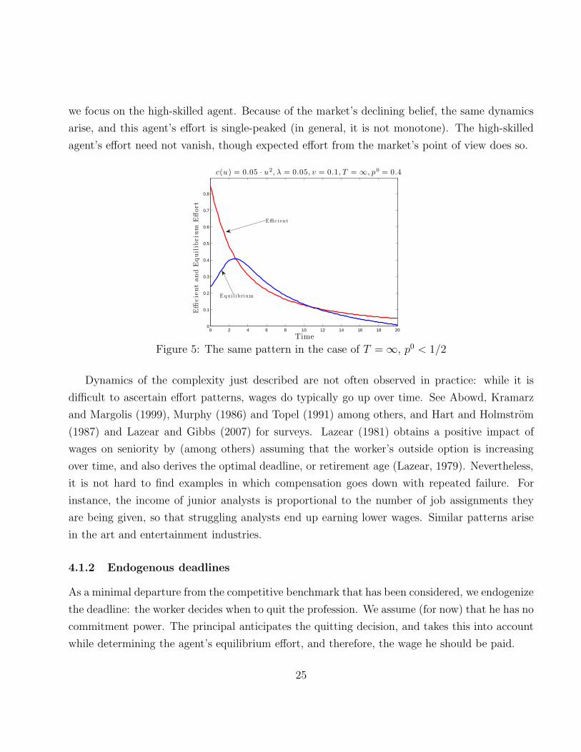
we focus on the high-skilled agent. Because of the market’s declining belief, the same dynamics
arise, and this agent’s effort is single-peaked (in general, it is not monotone). The high-skilled
agent’s effort need not vanish, though expected effort from the market’s point of view does so.
0 2 4 6 8 10 12 14 16 18 200
0.1
0.2
0.3
0.4
0.5
0.6
0.7
0.8
Time
Effi
cie
nt
and
Equil
ibri
um
Eff
ort
c(u) = 0.05 · u2, λ = 0.05, v = 0.1, T = ∞, p0 = 0.4
Effic i ent
Equi l i brium
Figure 5: The same pattern in the case of T = ∞, p0 < 1/2
Dynamics of the complexity just described are not often observed in practice: while it is
difficult to ascertain effort patterns, wages do typically go up over time. See Abowd, Kramarz
and Margolis (1999), Murphy (1986) and Topel (1991) among others, and Hart and Holmstrom
(1987) and Lazear and Gibbs (2007) for surveys. Lazear (1981) obtains a positive impact of
wages on seniority by (among others) assuming that the worker’s outside option is increasing
over time, and also derives the optimal deadline, or retirement age (Lazear, 1979). Nevertheless,
it is not hard to find examples in which compensation goes down with repeated failure. For
instance, the income of junior analysts is proportional to the number of job assignments they
are being given, so that struggling analysts end up earning lower wages. Similar patterns arise
in the art and entertainment industries.
4.1.2 Endogenous deadlines
As a minimal departure from the competitive benchmark that has been considered, we endogenize
the deadline: the worker decides when to quit the profession. We assume (for now) that he has no
commitment power. The principal anticipates the quitting decision, and takes this into account
while determining the agent’s equilibrium effort, and therefore, the wage he should be paid.
25

More specifically, in each interval [t, t+dt) such that the agent has not quit yet, the principal
pays a wage wtdt, then the agent decides how much effort to exert over this time interval, and
at the end of it, whether to stay or leave, an observable choice. This raises the issue of the
principal’s beliefs if the agent were to deviate and stay when expected to leave. For simplicity,
we adopt passive beliefs. That is, if the agent is supposed to drop out at some time but fails to,
the principal does not revise his belief regarding past effort choices, ascribing the failure to quit
to a mistake (this implies that he expects the agent to quit at the next opportunity).31
Endogenous deadlines do not affect the pattern of effort and wage. With convex cost, effort
is always decreasing at the deadline (i.e., at the agent’s optimal quitting time). This implies
that the wage is decreasing at the end (but not necessarily at the beginning). Hence, effort is
single-peaked and wages are first decreasing and then single-peaked. The belief at the deadline
is too high relative to the social planner’s at the first-best deadline. Furthermore, both effort
and the worker’s marginal product are decreasing throughout in the first-best solution.
How about if the worker could commit to the deadline (but still not to effort levels)? The
optimal deadline with commitment can be either shorter or longer than without. In either case,
however, the deadline is set so as to increase aggregate effort, and so increase wages. This may
require increasing the deadline –so as to increase the duration over which higher effort levels are
sustained, even if that means quitting at a point where staying is unprofitable– or decreasing the
deadline –so as to make high effort levels credible. Figure 6 illustrates the two possibilities.
We summarize our results in Proposition 4.3, the proof of which can be found in the working
paper.
Proposition 4.3 With convex cost,
1. effort is always decreasing at the optimal deadline without commitment;
2. the belief of the planner at the deadline is lower than the agent’s at the optimal deadline
without commitment;
3. the deadline with commitment can be shorter or longer than without.
31In the linear cost case, this means that we fix the off-equilibrium beliefs to specify ut = u if pt > p∗, where p∗
is the lowest belief at which it would be optimal for the agent to exert maximum effort if he anticipated quitting
at the end of the interval [t, t+dt) (see Appendix B for p∗ in closed-form), and ut = 0 otherwise. In other words,
the market does not react to a failure to quit, anticipates the agent quitting immediately afterwards and expects
instantaneous effort to be determined as if p = pT were the terminal belief.
26

0 0.5 1 1.5 2 2.5 3 3.5
0.85
0.9
0.95
1
1.05
1.1
1.15
1.2
1.25
1.3
Time
Effort
ut
c(u) = u2/2, v = 2, k = 3/2, λ = 1/50, p0 = 0.99
Commitment
No Commitment
0 0.5 1 1.5 2 2.5 3 3.5 4 4.5
0.7
0.8
0.9
1
1.1
1.2
1.3
1.4
Time
Effort
ut
c(u) = u2/2, v = 2, k = 7/2, λ = 1/50, p0 = 0.99
Commitment
No Commitment
Figure 6: Setting the deadline with commitment can push it higher or lower than without (the
curves stop at the respective deadlines).
4.2 Long-term contracts
Under spot contracts, the wage is equal to the worker’s marginal product. This is a reasonable
premise in a number of industries, in which lack of transparency or volatility in the firm’s revenue
stream might inhibit commitment by the firm to a particular wage scheme. Alternatively, it is
sometimes argued that competition for the agent’s services leads to a similar outcome. Our
model does not substantiate such a claim: if the principal can commit to a wage path, matters
change drastically, even under competition.
In particular, if the principal could commit to a breakthrough-contingent wage scheme, the
moral hazard problem would be solved entirely: under competition, the principal would offer the
agent the value of a breakthrough, 1, whenever a success occurs, and nothing otherwise.
If at least the principal could commit to a time-contingent wage scheme that involved pay-
ments after a breakthrough (with payments possibly depending on the agent staying with the
firm, but not on the realization of output), the moral hazard would also be mitigated. If promised
payments at time t in the case of no breakthrough are also made if a breakthrough has occurred,
all disincentives due to wages are eliminated.
Here, we examine a weaker form of commitment. The agent cannot be forced to stay with a
principal (he can leave at any time). Once a breakthrough occurs, the agent moves on (e.g., to a
different industry or position), and the firm is unable to retain him in this event. The principal
can commit to a wage path that is conditional on the agent working for her firm. Thus, wages
27

can only be paid in the continued absence of a breakthrough. Until a breakthrough occurs, other
firms, who are symmetrically informed (they observe the wages paid by all past employers),
compete by offering wage paths. The same deadline applies to all wage paths, i.e. the tenure
clock is not reset. For instance, the deadline could represent the agent’s retirement age, so that
switching firms does not affect the horizon.
For the remainder of this subsection, we restrict attention to the linear cost case. We write
the principal’s problem as of maximizing the agent’s welfare subject to constraints. Formally,
we solve the following optimization problem P.32 The principal chooses u : [0, T ] → [0, u] and
w : [0, T ] → R+, integrable, to maximize W (0, p0), where, for any t ∈ [0, T ],
W (t, pt) := maxw,u
∫ T
t
1− pt1− ps
(ws − v − αus) ds− k1− pt1− pT
,
such that, given w, the agent’s effort is optimal,
u = argmaxu
∫ T
t
1− pt1− ps
(ws − v − αus) ds− k1− pt1− pT
,
and the principal offers as much to the agent at later times than the competition could offer at
best, given the equilibrium belief,
∀τ ≥ t :
∫ T
τ
1− pτ1− ps
(ws − v − αus) ds− k1− pτ1− pT
≥ W (τ , pτ ) ; (10)
finally, the firm’s profit must be non-negative,
0 ≤
∫ T
t
1− pt1− ps
(ps(λ+ us)− ws)ds.
Note that competing principals are subject to the same constraints as the principal under con-
sideration: because the agent might ultimately leave them as well, they can offer no better than
W (τ , pτ) at time τ , given belief pτ . This leads to an “infinite regress” of constraints, with the
value function appearing in the constraints themselves. To be clear, W (τ , pτ) is not the con-
tinuation payoff that results from the optimization problem, but the value of the optimization
32We are not claiming that this optimization problem yields the equilibrium of a formal game, in which the
agent could deviate in his effort scheme, leave the firm, and competing firms would have to form beliefs about
the agent’s past effort choices, etc. Given the well-known modeling difficulties that continuous time raises, we
view this merely as a convenient shortcut. Among the assumptions that it encapsulates, note that there is no
updating based on an off-path action (e.g., switching principals) by the agent.
28

problem if it started at time τ .33 Because of the constraints, the solution is not time-consistent,
and dynamic programming is of little help. Fortunately, this problem can be solved, as shown in
Appendix C.2–at least as long as u and v are large enough. Formally, we assume that
u ≥( v
αλ− 1)
v − λ, and v ≥ λ(1 + k).34 (11)
Before describing its solution, let us provide some intuition. Recall the first-order condition
(5) that determines the agent’s effort. Clearly, the lower the future total wage bill, the stronger
the agent’s incentives to exert effort, which is inefficiently low in general. Now consider two times
t < t′: to provide strong incentives at time t′, it is best to frontload any promised payment to
times before t′, as such payments will no longer matter at that time. Ideally, the principal would
pay what he owes upfront, as a “signing bonus.” However, this violates the constraint (10), as
an agent left with no future payments would leave right after cashing in the signing bonus.
But from the perspective of incentives at time t, backloading promised payments is better.
To see this formally, note that the coefficient of the wage ws, s > t, in eqn. (5) is (up to the
factor (1− pt)) the likelihood ratio ps/ (1− ps), as explained before eqn. (5). Alternatively,
(1− pt)ps
1− ps= P [ω = 1|τ ≥ s]P [ω = 1] = P [ω = 1 ∩ τ ≥ s] ;
that is, effort at time t is affected by wage at time s > t inasmuch as time s is reached and the
state is 1: otherwise effort plays no role anyhow.
In terms of the firm’s profit (or the agent’s payoff), the coefficient placed on the wage at time
s (see (2)) is
P [τ ≥ s] ,
i.e., the probability that this wage is paid (or collected). Because players grow more pessimistic
over time, the former coefficient decreases faster than the latter: backloading payments is good
for incentives at time t. Of course, to provide incentives with later payments, those must be
increased, as a breakthrough might occur until then, which would void them; but it also decreases
the probability that these payments must be made in the same proportion. Thus, what matters
is not the probability that time s is reached, but the fact that reaching those later times is
33Harris and Holmstrom (1982) impose a similar condition in a model of wage dynamics under incomplete
information. However, because their model abstracts from moral hazard, constraint (10) reduces to a non-positive
continuation profit condition.34We do not know whether these assumptions are necessary for the result.
29

indicative of state 0, which is less relevant for incentives. Hence, later payments depress current
incentives less than earlier payments.
To sum up: from the perspective of time t, backloading payments is useful; from the point of
view of t′ > t , it is detrimental, but frontloading is constrained by (10). Note that, as T → ∞,
the planner’s solution tends to the agent’s best response to a wage of w = 0. Hence, the firm
can approach first best by promising a one-time payment arbitrarily far in the future (and wages
equal to marginal product thereafter). This would be almost as if w = 0 for the agent’s incentives,
and induce efficient effort. The lump sum payment would then be essentially equal to p0/(1−p0).
Note finally that, given the focus on linear cost, there is no benefit in giving the agent any
“slack” in his incentive constraint at time t; otherwise, by frontloading slightly future payments,
incentives at time t would not be affected, while incentives at later times would be enhanced.
Hence, the following result should come as no surprise.
Theorem 4.4 The following is a solution to the optimization problem P, for some t ∈ [0, T ].
Maximum effort is exerted up to time t, and zero effort is exerted afterwards. The wage is equal
to v−αλ up to time t, so that the agent is indifferent between all levels of effort up to then, and
it is 0 for all times s ∈ (t, T ); a lump-sum is paid at time T .35
The proof is in Appendix C.2, and it involves several steps: we first conjecture a solution in
which effort is first full (and the agent is indifferent), then nil; we relax the objective in program
P to maximization of aggregate effort, and constraint (10) to a non-positive continuation profit
constraint; we verify that our conjecture solves the relaxed program, and finally that it also
solves the original program. In the last step we show that (a) given the shape of our solution,
maximizing total effort implies maximizing the agent’s payoff, and (b) the competition constraint
(10) is slack at all times t > 0.
Hence, under one-sided commitment, high effort might be exerted throughout. This happens
if T is short and k > 0. When u is high enough (precisely, when (11) holds), the agent produces
revenue that exceeds the flow wage collected as time proceeds: the liability recorded by the
principal grows over time, shielding it from the threat of competition. This liability will eventually
be settled via a lump-sum payment at time T that can be interpreted as severance pay. If the
horizon is longer or k = 0, the lump-sum wipes out incentives close to the deadline, as in our
35The wage path that solves the problem is not unique in general.
30

introductory example, and effort is zero in a terminal phase. Thus, a phase with no effort exists
if and only if the deadline is long enough. The two cases are illustrated in Figure 7 below.
0 0.05 0.1 0.15 0.2 0.25
0
0.1
0.2
0.3
0.4
0.5
0.6
0.7
0.8
0.9
1
Time
Effort
,W
age
Paramet er s : α = 1/8 , v = 1/4 , λ = 1 , u = 1 , k = 1 , p0 = 0 .9 , T = 1/4
Wage w t
Effort u t
Severance pay
0 0.05 0.1 0.15 0.2 0.25 0.3 0.35 0.4 0.45 0.5
0
0.1
0.2
0.3
0.4
0.5
0.6
0.7
0.8
0.9
1
Time
Effort
,W
age
Parameters: α = 1/8, v = 1/4, λ = 1, u = 1, k = 1, p 0 = 0.9, T = 1/2
Wage w t
Severance pay
Effort u t
Figure 7: Wages and effort under commitment, for two horizon lengths.
As mentioned, all these results are proved for the case of linear cost. It is all the more
striking that the result obtains in this “linear” environment. Indeed, rigidity and severance pay
are usually attributed to risk aversion by the agent (see Azariadis, 1975, among many others).
Commitment provides an alternative rationale.
Nonetheless, it is desirable to know to which extent the findings are valid for general cost
specification. Our earlier numerical example with quadratic costs (Figure 1 in the introduction)
provides some important hints. In general, the equilibrium involves two phases: in a first phase,
the agent is paid his marginal product; in a second phase, he is not paid at all, and the excess
product of his effort is backloaded into a final lump payment. If the horizon is long enough, the
phase in which wages are equal to marginal product disappears and all payments are backloaded.
If the horizon is very short and k is low enough, the backloading phase disappears, and the
structure is then identical to spot contracts: the agent is paid his marginal product throughout.
The principal faces a simple choice: paying as soon as possible, which requires setting the
wage equal to the marginal product to satisfy the no-poaching constraint; or backloading en-
tirely. Early payments are bad for current incentives, but best for later incentives because these
payments will be sunk by then; backloading is best for current incentives, but depresses later
incentives. Depending on the horizon length, one or the other solution is chosen. If the horizon
is very long, backloading takes over: by the time the deadline is near, the principal already owes
31

the worker a large enough amount that the competition constraint is ineffective even though the
large payment promised at the deadline eliminates the incentives to work close to T .
However, full backloading is not the solution if the relationship begins close to the deadline:
with a very short horizon, the imminent lump-sum payment reduces the agent’s incentives to
work, and hence the marginal product. Then there is not enough time for the principal to
accumulate a liability sufficient to make his contract immune to poaching. The principal can
then do no better than offer a contract replicating spot wages, which is immune to itself.36
To sum up, with a long horizon, commitment alleviates the unavoidable delay in effort provi-
sion that comes with compensating a worker for persistent failure by backloading compensation.
5 Robustness
Undoubtedly, our model has stylized features. Output is not observed at all; all uncertainty is
resolved after one breakthrough, there is no learning-by-doing, and the quality of the project
cannot change over time. We start discussing the case in which effort is observable. Predictably,
this changes conclusions significantly. We then briefly consider three variations (multiple break-
throughs, learning-by-doing, changing types), each of which embeds our baseline model as a
special case. We argue that none of these features is critical to our main findings.
5.1 Observable effort
The inability to contract on effort might be attributable to the subjectivity in its measurement
rather than to the impossibility of monitoring it. Co-workers usually have a fairly good idea of
their colleagues’ work ethic. The evaluation of a worker’s immediate superior affects his future
compensation. To understand incentives in such an environment, we assume here that effort is
observed. We revert to spot contracts: the firm pays upfront the value of output. Because effort
is monitored, the firm and agent beliefs coincide on and off path. The flow wage is given by
wt = pt(λ+ ut),
36The only difference with the linear case is that, with linear cost, a constant flow wage w = v−αλ induces the
agent to exert maximal effort and generates positive flow profits for the firm. Thus, there is always some excess
marginal product that gets backloaded. This allows the principal to accumulate sufficient liabilities even with
short horizons. If, in addition, k is sufficiently large, the agent can be induced to exert maximal effort throughout.
32

where pt is the belief and ut is expected effort. We assume linear cost. The agent maximizes
V (p0, 0) :=
∫ T
0
1− p01− pt
[pt(λ+ ut)− αut − v] dt− k1− p01− pT
.
In contrast to (2), the revenue is no longer a function of time only, as effort affects future beliefs,
thus wages. Hence, effort is a function of t and p. We focus on equilibria in Markov strategies
u : [0, 1]× [0, T ] → [0, u] ,
such that u(p, t) is upper semi-continuous and the value function V (p, t) piecewise differentiable.37
Lemma 5.1 Fix a Markov equilibrium. If u = 0 on some open set Ω ⊂ [0, 1]× [0, T ], then also
u (p′, t′) = 0 if the equilibrium trajectory that starts at (p′, t′) intersects Ω.
Hence, if the agent ever exerts effort, he is willing to do so at any later time (on path). Thus, in
any equilibrium involving extremal effort levels only, there are at most two phases: the worker
exerts no effort, and then full effort. This is the opposite of the socially optimal policy, which
frontloads effort (see Lemma 2.1). The agent can only be trusted to put in effort if he is “back to
the wall,” so that effort remains optimal at any later time, no matter what he does; if the market
paid for effort, yet the agent was expected to let up later on, then he would gain by deviating to
no effort, pocketing the high wage in the process; because such a deviation makes everyone more
optimistic, it would only increase his incentives to exert effort (and so his wage) at later times.
This does not imply that the equilibrium is unique, as the next theorem establishes.
Theorem 5.2 Given T > 0, there exists continuous, distinct, non-increasing p, p : [0, T ] →
[0, 1], with pt≤ pt and p
T= pT , such that:
1. all Markov equilibria involve maximum effort above p:
pt > pt ⇒ u (p, t) = u;
2. all Markov equilibria involve no effort below p:
pt ≤ pt⇒ u (p, t) = 0;
37That is, there exists a partition of [0, 1] × [0, T ] into closed Si with non-empty interior, such that V is
differentiable on the interior of Si, and the intersection of any Si, Sj is empty or a smooth 1-dimensional manifold.
33
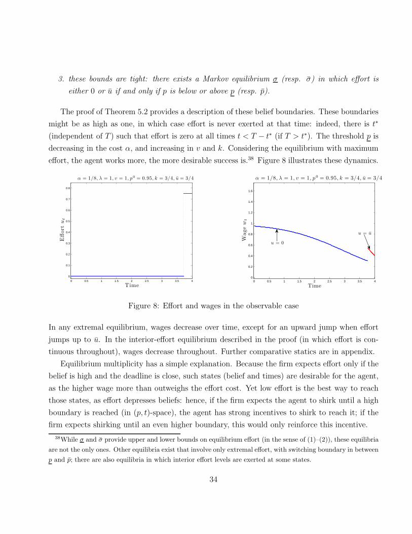
3. these bounds are tight: there exists a Markov equilibrium σ (resp. σ) in which effort is
either 0 or u if and only if p is below or above p (resp. p).
The proof of Theorem 5.2 provides a description of these belief boundaries. These boundaries
might be as high as one, in which case effort is never exerted at that time: indeed, there is t∗
(independent of T ) such that effort is zero at all times t < T − t∗ (if T > t∗). The threshold p is
decreasing in the cost α, and increasing in v and k. Considering the equilibrium with maximum
effort, the agent works more, the more desirable success is.38 Figure 8 illustrates these dynamics.
0 0.5 1 1.5 2 2.5 3 3.5 4
0
0.1
0.2
0.3
0.4
0.5
0.6
0.7
0.8
Time
α = 1/8, λ = 1, v = 1, p0 = 0.95, k = 3/4, u = 3/4
Effort
ut
0 0.5 1 1.5 2 2.5 3 3.5 40
0.2
0.4
0.6
0.8
1
1.2
1.4
1.6
Time
Wage
wt
α = 1/8, λ = 1, v = 1, p0 = 0.95, k = 3/4, u = 3/4
u = u
u = 0
Figure 8: Effort and wages in the observable case
In any extremal equilibrium, wages decrease over time, except for an upward jump when effort
jumps up to u. In the interior-effort equilibrium described in the proof (in which effort is con-
tinuous throughout), wages decrease throughout. Further comparative statics are in appendix.
Equilibrium multiplicity has a simple explanation. Because the firm expects effort only if the
belief is high and the deadline is close, such states (belief and times) are desirable for the agent,
as the higher wage more than outweighs the effort cost. Yet low effort is the best way to reach
those states, as effort depresses beliefs: hence, if the firm expects the agent to shirk until a high
boundary is reached (in (p, t)-space), the agent has strong incentives to shirk to reach it; if the
firm expects shirking until an even higher boundary, this would only reinforce this incentive.
38While σ and σ provide upper and lower bounds on equilibrium effort (in the sense of (1)–(2)), these equilibria
are not the only ones. Other equilibria exist that involve only extremal effort, with switching boundary in between
p and p; there are also equilibria in which interior effort levels are exerted at some states.
34

Let us turn to a comparison with the case of non-observable effort, as described in subsection
4.1. Along the equilibrium path, the dynamics of effort look very different when one compares
the social planner’s solution to the agent’s optimum under either observability assumption. Yet
effort can be ranked across those cases. To do so, the key is to describe effort in terms of the state
(p, t), i.e., the public belief and calendar time. In all equilibria, effort is lower under observability.
Proposition 5.3 The maximum effort region for the observable case is contained in the full
effort region(s) for the non-observable case.
This confirms that observability depresses incentives: the highest effort equilibrium with observ-
ability entails less effort than without. Recall from Proposition 3.4 that the (interior or full) effort
region in the non-observable case is itself contained in the effort region for the social planner.
Having the worker quit when it is best for him (without commitment to the deadline) rein-
forces our comparison between observable and non-observable effort.39
5.2 Multiple breakthroughs
Suppose that one success does not resolve all uncertainty. Specifically, there are three states,
ω = 0, 1, 2, two consecutive projects, and an infinite horizon. The first one can be completed if
and only if the state is not 0 ; assume arrival rates of λ1+ut and λ2+ut, respectively, conditional
on ω = 1, 2; if the first project is completed, an observable event, the agent tackles the second,
which can be completed only if ω = 2; assume again an arrival rate of λ2 + ut if ω = 2.
Such an extension can be solved by “backward induction.” Once the first project is completed,
the continuation game reduces to the game of Section 4. The value function of this problem then
serves as continuation payoff to the first stage. While this value function cannot be solved in
closed-form, it is easy to derive the solution numerically. The following example illustrates the
structure of the solution. The parameters are v = 1, α = 1/2,P[ω > 0] = 0.85,P[ω = 2 | ω > 0] =
0.75, λ2 = 1, λ1 = 0.6, c(u) = u2/8. See Figure 9. The left panel shows effort and wages during
the first stage. As is clear, the same pattern as in our model emerges: effort is single-peaked,
and as a result, wages can be first decreasing, then single-peaked.
39See the working paper for details. Non-Markov equilibria exist. Defining them in our environment is prob-
lematic, but it is clear that threatening the agent with reversion to the Markov equilibrium σ provides incentives
for effort extending beyond the high-effort region defined by σ –in fact, beyond the high-effort region in the
unobservable case. The planner’s solution remains out of reach, as punishments are restricted to beliefs below p.
35

The right panel shows how efforts and beliefs evolve before and after the first success. The
green curves represent the equilibrium belief that ω = 2, before and after the success (the light
green curve is the belief as long as no success has occurred, and the dark green one the belief
right after a success has occurred); the blue curves are equilibrium effort (the light blue curve is
effort as long as no success has occurred, the dark blue one is the effort right after a success).
Note that effort at the start of the second project is also single-peaked as a function of the time
at which this project is started (the later it is started, the more pessimistic the agent at that
stage, though his belief has obviously jumped up given the success).
0 1 2 3 4 5 6 70
0.1
0.2
0.3
0.4
0.5
0.6
0.7
0.8
0.9
1
Time
Eff
ort
u1
,t,w
age
w1
,t
u 1 , t
w 1 , t
0 1 2 3 4 5 6 70
0.1
0.2
0.3
0.4
0.5
0.6
0.7
0.8
0.9
1
Time
Eff
ort
ui,t,bel
iefs
pi,t
u 2 , t
u 1 , t
p 2 , t
p 1 , t
Figure 9: Efforts and beliefs with two breakthroughs
5.3 Learning-by-doing
Memorylessness is a convenient but stark property of the exponential distribution. It implies that
past effort plays no role in the probability of instantaneous breakthrough. In many applications,
agents learn from the past not only about their skill levels, but about the best way to achieve a
breakthrough. While a systematic analysis of learning-by-doing is beyond the scope of this paper,
we can gain some intuition from numerical simulations. We model human capital accumulation
as in Doraszelski (2003). The evolution of human capital is given by
zt = ut − δzt, z0 = 0,
while its productivity is
ht = ut + ρzφt .
36

That is, the probability of success over the interval [t, t + dt) is (λ+ ht)dt, given human capital
ht and effort ut. Here δ, ρ and φ are positive constants that measure how fast human capital
depreciates, its importance relative to instantaneous effort, and the returns to scale from human
capital.40
Figure 10 illustrates the results. Not surprisingly, the main new feature is a spike of effort
at the beginning, whose purpose is to build human capital. This spike might lead to decreasing
initial effort, before it becomes single-peaked, though this need not be the case. Beyond this new
twist, features from the baseline model appear quite robust.
0 1 2 3 4 5 6 7 80
0.1
0.2
0.3
0.4
0.5
0.6
0.7
0.8
Time
c (u ) = u 2/4, k = 1/3, λ = 1/2, v = 2/3, p 0 = 0.95, ρ = 4, φ = 1, δ = 0
Effort
ut
and
wage
wt
Wage
Effort
0 1 2 3 4 5 6 7 80
0.1
0.2
0.3
0.4
0.5
0.6
0.7
0.8
Time
Effort
ut
and
wage
wt
c (u ) = u 2/4, k = 1/3, λ = 1/2, v = 2/3, p 0 = 0.95, ρ = 1, φ = 1, δ = 0
Wage
Effort
Figure 10: Two possible configurations with learning-by-doing
5.4 Changing state
Suppose finally that, unbeknownst to the agent and the principal, the state of the world is reset
at random times, exponentially distributed at rate ρ > 0; whenever it is reset, the state is reset
to 1 with probability p∗ ∈ (0, 1).41 This is the counterpart of the stationary version of Holmstrom
for Gaussian noise. Specifically, suppose that with instantaneous probability ρ > 0 the ability is
40Cisternas (2012b) introduces human-capital accumulation in the Holmstrom framework by letting the agent’s
skill follow a diffusion with an endogenous drift component.41This specification bears a close similarity to Board and Meyer-ter-Vehn (2010, 2013), though it also differs
in some key respects; among others, the state-resetting process is exogenous and information is symmetric (on
path).
37

reset, in which case it is high with probability p∗. Such an event is unobserved by all parties. As
before, a breakthrough ends the game, and the environment remains the same as before, with
linear cost (and v > αλ, as before) and an infinite horizon. (Thus, the baseline model with linear
cost and T = ∞ is a special case in which ρ = 0.) By Bayes’ rule, the (agent’s) belief p obeys
pt = ρ (p∗ − pt)− pt (1− pt) (λ+ ut) , p0 = p0,
and this is the same as the principal’s belief in equilibrium. The equilibrium is unique, and effort
and belief converge to some limiting value, which is independent of the prior, and decreasing in
the eventual effort level u, as follows. (The proof of the following is available from the authors.)
Proposition 5.4 There exists αλ < v < v and 0 < p < p < p∗ such that, if:
1. v > v, effort is eventually maximum, and p tends to a limit below p;
2. v ∈ (v, v), effort is eventually interior, with p tending to a limit in (p, p);
3. v < v, effort is eventually zero, and p tends to a limit above p.
The higher the value, the more effort is exerted, the lower is the asymptotic belief. This eventual
belief is non-decreasing in p∗ and ρ and non-increasing in u. It is decreasing in λ when effort
is extremal, but increasing otherwise. Asymptotic effort (or stationary effort if p0 = p∗) is
decreasing in α, the marginal cost of effort, and in λ, the “luck” component of the arrival of
breakthroughs. Comparative statics of effort with respect to p∗ and ρ are ambiguous.
Note that, if the prior belief is below the limiting value, effort and hence wage can be increasing
over time. (It is easy to construct examples in which wage increases throughout, see right panel
of Figure 11, but it need not be so, see left panel.) It would be interesting to consider the game
that does not end with a success, but rather continues with a value reset at the prior of 1 (which
immediately starts declining towards p∗), but we have not pursued this here.
6 Concluding remarks
There are several extensions that we think could potentially yield interesting insights.
38

0 1 2 3 4 5 6 7 8 9 100
0.1
0.2
0.3
0.4
0.5
0.6
0.7
0.8
0.9
Time
Effort
ut
and
bel
iefs
pt
α = 1/5, λ = 1/2, v = 1/2, p 0 = 0.9, u = 2, ρ = 1/3, p ∗ = 0.7
Belie f s
Effort
0 1 2 3 4 5 6 7 8 9 100.05
0.1
0.15
0.2
0.25
0.3
Time
α = 1/5, λ = 1/2, v = 1/2, p 0 = 0.27, u = 2, ρ = 1/3, p ∗ = 0.7
Effort
ut
and
bel
iefs
pt
Belie f s
Effort
Figure 11: Changing states: two possible configurations
Policy Design We have not touched upon the issue of corrective measures that can be taken
to remedy the inefficiency of the different market structures that have been considered. Various
arrangements could be studied, that differ in terms of flexibility and coerciveness: taxes, pensions,
or even, in the extreme case, slavery, etc. For instance, an obvious institution to examine within
our framework is apprenticeship length (see Malcomson, Maw and McCormick, 2003).
Search equilibrium We have not addressed either the optimal timing for a firm to lay off
the worker. To examine this issue, it is necessary to introduce some frictions: with short-run
contracts, the firm breaks even at all times, so that it has nothing to lose or gain by firing the
worker. Yet this is an important question, in light of the rigid tenure policies adopted by many
professional service firms. Why not keep the employee past the probationary period, adjusting
the wage for the diminished incentives and lower assessed ability?42 Firms have a cost of hiring
(or firing) workers –possibly due to the delay in filling a vacancy– but derive a surplus in excess
of the competitive wage. Studying the efficiency properties and the characteristics of the labor
market (composition of the working force, duration of unemployment) would be an interesting
undertaking. A natural starting point would be a market in which marginal productivities are
heterogenous, and there are matching frictions, as in Postel-Vinay and Robin (2002).
42See Gilson and Mnookin (1989) for a discussion of this puzzle for the case of law firms.
39

Partnerships Our framework is suitable for an analysis of reputation in partnerships, which
is relevant for professional service firms. In law or consulting, projects are assigned to teams,
combining partners with junior associates. The team pursues conflicting objectives: incentivizing
both partner and associate, and eliciting information about the associate’s ability. How should
profits be shared? Is it optimal to combine workers whose assessed abilities differ?
Another issue is yardstick competition: here, there is no distinction between the agent’s skill
and the project’s feasibility. In practice, the market learns about both. This also occurs through
the progress of other agents’ work on related tasks. Yardstick competition affects incentives.
Relatedly, workers of different perceived skills might choose different types of projects; more
challenging projects, or tougher environments, might foster learning of very high skilled workers,
but be redhibitory for workers with lower perceived skills. Examining how the market allocates
employees and firms, and how this differs from the efficient match is an interesting problem.
References
Abowd, J.M., F. Kramarz and D.N. Margolis, 1999. “High wage workers and high wage firms,”
Econometrica, 67, 251–333.
Azariadis, C., 1975. “Implicit Contracts and Underemployment Equilibria,” Journal of Political
Economy, 83, 1183–1202.
Bar-Isaac, H., 2003. “Reputation and Survival: learning in a dynamic signalling model,” Review
of Economic Studies, 70, 231–251.
Bergemann, D. and U. Hege, 2005. “The Financing of Innovation: Learning and Stopping,”
RAND Journal of Economics, 36, 719–752.
Board, S. and M. Meyer-ter-Vehn, 2010. “A Reputational Theory of Firm Dynamics,” working
paper, UCLA.
Board, S. and M. Meyer-ter-Vehn, 2013. “Reputation for Quality,” Econometrica, forthcoming.
Caves, R.E., 2003. “Contracts Between Art and Commerce,” Journal of Economic Perspectives,
17, 73–83.
40

Cesari, L., 1983. Optimization: Theory and Applications. Problems with ordinary differential
equations, Applications of Mathematics, 17, Berlin-Heidelberg-New York: Springer-Verlag.
Chevalier, J. and G. Ellison, 1999. “Career Concerns of Mutual Fund Managers,” Quarterly
Journal of Economics, 114, 389–432.
Chisholm, D. C., 1997. “Profit-Sharing versus Fixed-Payment Contracts: Evidence from the
Motion Pictures Industry,” Journal of Law, Economics & and Organization, 13, 169–201.
Cisternas, G., 2012a. “Two-sided Learning and Moral Hazard,” working paper, Princeton Uni-
versity.
—, 2012b. “Shock Persistence, Endogenous Skills and Career Concerns,” working paper, Prince-
ton University.
Cockburn, B., Henderson, R. and S. Stern, 1999. “Balancing Incentives in Pharmaceutical
Research,” National Bureau of Economic Research, working paper.
Dewatripont, M., I. Jewitt and J. Tirole, 1999a. “The Economics of Career Concerns, Part I:
Comparing Information Structures,” Review of Economic Studies, 66, 183–198.
Dewatripont, M., I. Jewitt and J. Tirole, 1999b. “The Economics of Career Concerns, Part
II: Application to Missions and Accountability of Government Agencies,” Review of Economic
Studies, 66, 199–217.
Doraszelski, U., 2003. “An R&D race with knowledge accumulation,” RAND Journal of Eco-
nomics, 34, 20–42.
Ethiraj, S. and M. Zhao, 2012. “Lemons, stars, and startups: A study of scientist departures
following project termination in the pharmaceutical industry,” working paper, University of
Michigan.
Fama, E., 1980. “Agency Problems and the Theory of the Firm,” Journal of Political Economy,
88, 288–307.
Fama, E. and M. Jensen, 1983. “Separation of Ownership and Control,” Journal of Law and
Economics, 26, 301–325.
41

Ferrer, R., 2011. “The Effect of Lawyers’ Career Concerns on Litigation,” working paper, Uni-
versitat Pompeu Fabra.
Ghosh, S. and M. Waldman, 2010. “Standard promotion practices versus up-or-out contracts,”
RAND Journal of Economics, 41, 301–325.
Gibbons, R. and K. J. Murphy, 1992. “Optimal Incentive Contracts in the Presence of Career
Concerns: Theory and Evidence,” Journal of Political Economy, 100, 468–505.
Gilson, R.J. and R.H. Mnookin, 1989. “Coming of Age in a Corporate Law Firm: The Economics
of Associate Career Patterns,” Stanford Law Review, 41, 567–595.
Gittelman, M. and B. Kogut, 2003. “Does Good Science Lead to Valuable Knowledge? Biotech-
nology Firms and the Evolutionary Logic of Citation Patterns,” Management Science, 49, 366–
382.
Goodman, M., 2013. “Banker bonuses for Glaxo boffins,” The Sunday Times, available at
http://www.thesundaytimes.co.uk/sto/business/Companies/article1277520.ece.
Harris, M. and B. Holmstrom, 1982. “A Theory of Wage Dynamics,” Review of Economic
Studies, 49, 315–333.
Hart, O. and B. Holmstrom, 1987. “A Theory of Contracts,” in Advances in Economic Theory,
Fifth World Congress, ed. by Truman F. Bewley. Cambridge: Cambridge University Press,
71–155.
Holmstrom, B., 1999. “Managerial Incentive Problems: a Dynamic Perspective,” Review of
Economic Studies, 66, 169–182. (Originally published in 1982 in Essays in Honor of Professor
Lars Wahlbeck.)
Johnson, E.M., 2011. “Ability, Learning and the Career Path of Cardiac Specialists,” working
paper, MIT Sloan School of Management.
Jovanovic, B., 1979. “Job Matching and the Theory of Turnover,” Journal of Political Economy,
87, 972–990.
42

Kolstad, J., 2013. “Information and Quality when Motivation is Intrinsic: Evidence from Sur-
geon Report Cards,” American Economic Review, forthcoming.
LaMattina, J., 2012. “A Brief History of Tofacitinib,” Forbes, available at
http://www.forbes.com/sites/johnlamattina/2012/05/10/a-brief-history-of-tofacitinib/.
Lazear, E., 1979. “Why Is There Mandatory Retirement?” Journal of Political Economy, 87,
1261–1284.
—, 1981. “Agency, Earnings Profiles, Productivity, and Hours Restrictions,” American Eco-
nomic Review, 71, 606–620.
Lazear, E. and M. Gibbs, 2007. Personnel Economics for Managers. New York: John Wiley
and Sons.
Mailath, G.J. and L. Samuelson, 2001. “Who Wants a Good Reputation?,” Review of Economic
Studies, 68, 415–441.
Malcomson, J., J. W. Maw and B. McCormick, 2003. “General training by firms, apprentice
contracts, and public policy,” European Economic Review, 47, 197–227.
Murphy, K.J., 1986. “Incentives, Learning, and Compensation: A Theoretical and Empirical
Investigation of Managerial Labor Contracts,” RAND Journal of Economics, 17, 59–76.
PhRMA, 2012. “Pharmaceutical Industry: Profile 2012,” The Pharmaceutical Research and
Manufacturers of America, Washington, D.C.
Postel-Vinay, F. and J.-M. Robin, 2002. “Equilibrium Wage Dispersion with Worker and Em-
ployer Heterogeneity,” Econometrica, 70, 2295–2350.
Pray, L., 2008. “Gleevec: the breakthrough in cancer treatment,” Nature Education, 1.
Prendergast, C. and L. Stole, 1996. “Impetuous youngsters and jaded oldtimers,” Journal of
Political Economy, 104, 1105–34.
Seierstad, A. and K. Sydsæter, 1987. Optimal Control Theory with Economic Applications.
North-Holland.
43

Shaywitz, D., 2013. “You Just Don’t Understand (R&D),” Forbes, available at
http://www.forbes.com/sites/davidshaywitz/2013/07/17/you-just-dont-understand-rd/.
Stern, S., 2004. “Do Scientists Pay to Be Scientists?,” Management Science, 50, 835–853.
Topel, R., 1991. “Specific Capital, Mobility and Wages: Wages Rise with Job Seniority,” Journal
of Political Economy, 99, 145–176.
Trajtenberg, M., Shiff, G. and R. Melamed, 2006. “The “names game”: harnessing inventors’
patent data for economic research,” working paper, National Bureau of Economic Research.
Zucker, L. and M. Darby, 1996. “Star scientists and institutional transformation: Patterns of
invention and innovation in the formation of the biotechnology industry,” Proceedings of the
National Academy of Sciences, 93, 12709–12716.
44

Appendix
Throughout this appendix, we shall use the log-likelihood ratio
xt := ln1− ptpt
of state ω = 0 vs. ω = 1. We set x0 := ln(1 − p0)/p0. Note that x increases over time and, given u, follows the
O.D.E.
xt = λ+ ut,
with x0 = x0. We shall also refer to xt as the “belief,” hoping that this will create no confusion.
We start by explaining how the objective function can be derived as the limit of a discounted version of our
problem. Suppose that V is the value of a success and VL = V − k is the value of failure. Given the discount rate
r, the agent’s payoff is given by
(1 + e−x0
)V0 =
∫ T
0
e−rt(1 + e−xt
)(
xt1 + ext
V + wt − c (ut)
)
dt+ e−rT(1 + e−xT
)VL,
where V0 is his ex ante payoff.
Integrating by parts we obtain
(1 + e−x0
)V0 =
∫ T
0
e−rte−xtxtV dt+
∫ T
0
e−rt(1 + e−xt
)(wt − c (ut)) dt+ e−rT
(1 + e−xT
)(V − k)
= −e−rte−xtV∣∣T
0+
∫ T
0
e−rt((1 + e−xt
)(wt − c (ut))− e−xtrV
)dt+ e−rT
(1 + e−xT
)(V − k)
= e−x0V − e−rT e−xTV +
∫ T
0
e−rt(1 + e−xt
)(
wt − c (ut)−rV
1 + ext
)
dt+ e−rT(1 + e−xT
)(V − k) ,
so that as r → 0 (and defining v as rV → v) we obtain
(1 + e−x0
)(V0 − V ) =
∫ T
0
(1 + e−xt
)(
wt − c (ut)−v
1 + ext
)
dt− k(1 + e−xT
).
Similarly, one can show the social planner’s payoff is given by
(1 + e−x0
)(V0 − V )− e−x0 + k = −
∫ T
0
(1 + e−xt
)(
c (ut) +v
1 + ext
)
dt− (1 + k) e−xT .
A Proofs for Section 2
Proof of Lemma 2.1. In both the linear and convex cases, existence and uniqueness of a solution follow as
special case of Lemma 3.1, when w = 0 identically (the transversality condition must be adjusted). To see that
45

the social planner’s problem is equivalent to this, note that (whether the cost is convex or linear), the “revenue”
term of the social planner’s objective satisfies
∫ T
0
(1 + e−xt)λ+ ut1 + ext
dt =
∫ T
0
xte−xtdt = e−x0
− e−xT ,
and so this revenue only affects the necessary conditions through the transversality condition at T .
Let us start with the linear case. The social planner maximizes
∫ T
0
(1 + e−xt)
(λ+ ut1 + ext
− αut − v
)
dt− ke−xT , s.t. xt = λ+ ut.
We note that the maximization problem cannot be abnormal, since there is no restriction on the terminal value
of the state variable. See Note 5, Ch. 2, Seierstad and Sydsæter (1987). The same holds for all later optimization
problems.
It will be understood from now on that statements about derivatives only hold almost everywhere.
Let γt be the costate variable. The Hamiltonian for this problem is
H (x, u, γ, t) = e−xt(λ+ ut)− (1 + e−xt)(v + αut) + γt (λ+ ut) .
Define φt := ∂H/∂ut = (1 − α)e−xt − α+ γt. Note that given xt and γt, the value of φt does not depend on ut.
Pontryagin’s principle applies, and yields
ut = u (ut = 0) ⇔ φt :=∂H
∂ut= (1− α)e−xt − α+ γt > (<)0,
as well as
γt = e−xt(λ− v + (1− α)ut), γT = ke−xT .
Differentiating φt with respect to time, and using the last equation gives
φt = e−xt(αλ− v), φT = (1 + k − α)e−xT − α.
Note that φ is either increasing or decreasing depending on the sign of αλ−v. Therefore, the planner’s solution is
either maximum effort–no effort, or no effort–maximum effort, depending on the sign of this expression. Finally,
the marginal product p (λ+ u) is decreasing if effort maximum–zero. If effort is zero–maximum, the marginal
product is decreasing, jumps up, and then decreases again.
Consider now the convex case. Applying Pontryagin’s theorem (and replacing the revenue term by its ex-
pression in terms of xt and x0, as explained above) yields as necessary conditions
γt = −e−x(c(u) + v), γt = (1 + e−xt)c′(ut),
where γt is the co-state variable, as before. Differentiate the second expression with respect to time, and use the
first one to obtain
u =(λ+ u) c′ (u)− c (u)− v
c′′ (u) (1 + ex), (12)
46

in addition to x = λ+ u (time subscripts will often be dropped for brevity). Let
φ (u) := (λ+ u) c′ (u)− c (u)− v.
Note that φ (0) = −v < 0, and φ′ (u) = (λ+ u) c′′ (u) > 0, and so φ is strictly increasing and convex. Let u∗ ≥ 0
be the unique solution to
φ (u∗) = 0,
and so φ is negative on [0, u∗] and positive on [u∗,∞). Accordingly, u < u∗ =⇒ u < 0, u = u∗ =⇒ u = 0 and
u > u∗ =⇒ u > 0. Given the transversality condition
(1 + exT ) c′ (uT ) = 1 + k,
we can then define xT(x0)by
xT (x0) =
1
λ+ u∗
[
ln
(1 + k
c′ (u∗)− 1
)
− x0]
,
and so effort is decreasing throughout if xT > xT (x0), increasing throughout if xT < xT (x
0), and equal to u∗
throughout otherwise. The conclusion then follows from the proof of Lemma 2.3, which establishes that the belief
xT at the deadline is increasing in T .
We now turn to the marginal product p (λ+ u). In terms of x, the marginal product is given by
w (x) :=λ+ u (x)
1 + ex, and so
w′ (x) =u′ (x)
1 + ex− w (x)
ex
(1 + ex),
so that w′ (x) = 0 is equivalent to
u′ (x) = w (x) ex.
Notice that u′ (x) ≤ 0 implies w′ (x) < 0. Conversely, if u′ (x) > 0, consider the second derivative of w (x). We
have
w′′ (x) = −ex
1 + exw′ (x) +
1
1 + ex(u′′ (x)− w (x) ex − u′ (x) ex) ,
so that when w′ (x) = 0 we have
w′′ (x) =u′′ (x)− u′ (x)
1 + ex.
From equation (12) we obtain an expression for the derivative of u with respect to x:
u′ (x) =(λ+ u) c′ (u)− c (u)− v
c′′ (u) (1 + ex) (λ+ u).
47

Let g (u) = v + c (u)− (λ+ u) c′ (u) and study u′′ (x) when w′ (x) = 0. We have
u′′ (x) =u′
1 + ex+g ((1 + ex) (c′′ + (λ+ u) c′′′)u′ (x) + exc′′ (λ+ u))
(c′′ (u) (1 + ex) (λ+ u))2
=c′′ (λ+ u)u′ (x)
c′′ (1 + ex) (λ+ u)−u′ (x) ((1 + ex) (c′′ + (λ+ u) c′′′) u′ (x) + exc′′ (λ+ u))
c′′ (1 + ex) (λ+ u)
= −u′ (x) ((1 + ex) (c′′ + (λ+ u) c′′′)u′ (x) + exc′′ (λ+ u)− c′′ (λ+ u))
c′′ (1 + ex) (λ+ u)
= −u′ (x) ((2c′′ + (λ+ u) c′′′) ex (λ+ u)− c′′ (λ+ u))
c′′ (1 + ex) (λ+ u).
We therefore consider the quantity
u′′ (x) − u′ (x) = −u′ (x) ((2c′′ + (λ+ u) c′′′) ex − c′′ + c′′ (1 + ex))
c′′ (1 + ex)
= −u′ (x) (3c′′ + (λ+ u) c′′′) ex
c′′ (1 + ex)< 0,
if as we have assumed, c′′+(λ+ u) c′′′ > 0. Therefore, we have a single-peaked (at most increasing then decreasing)
marginal product.
Proof of Lemma 2.3. We shall use the necessary conditions obtained in the previous proof. Part (1) is almost
immediate. Note that in both the linear and convex case, the necessary conditions define a vector field (u, x),
with trajectories that only define on the time left before the deadline and the current belief. Because trajectories
do not cross (in the plane (−τ, x), where τ is time-to-go and x is the belief), and belief x can only increase with
time, if we compare two trajectories starting at the same level x0, the one that involves a longer deadline must
necessarily involve as high a terminal belief x as the other (as the deadline expires).
(2) In the linear case, it is straightforward to solve for the switching time (or switching belief) under As-
sumption 2.2. For all terminal beliefs xT > x∗, for which no effort is exerted at the deadline, the switching belief
between equilibrium phases is determined by
(1 + k − α)e−xT − α =
∫ xT
x
e−sαλ− v
λds,
which gives as value of x (as a function of t)
x (t) = ln(
(1 + k − v/λ)e−λ(T−t) − (α− v/λ))
− lnα.
This represents a frontier in (t, x) space that the equilibrium path will cross from below for sufficiently long
deadlines. Consistent with the fact that, in the optimum, a switch to zero effort is irreversible, when ut = 0 and
xt = λ, the path leaves this locus (i.e., it holds that x′ (t) < λ).
The switching belief x (t) decreases in T : the longer the deadline, the longer maximum effort will be exerted
(recall that x measures pessimism). This belief decreases in α and increases in v and k: the higher the cost of
failing, or the lower the cost of effort, the longer effort is exerted. These are the comparative statics mentioned
in the text before Lemma 2.3.
48

Furthermore, by differentiating, the boundary x(·) satisfies x′(t) < 0 (resp. > 0) if and only if 1 + k < v/λ.
In that case, total effort increases with T : considering the plane (−τ , x), where τ is time-to-go and x is the belief,
increasing the deadline is equivalent to increasing τ , i.e. shifting the initial point to the left; if x′ < 0, it means
that the range of beliefs over which high effort is exerted (which is 1-to-1 with time spent exerting maximum effort,
given that x = λ+ u) increases. If instead x′ is positive, total effort decreases with T , by the same argument.
Consider now the convex case. Note that
1
x′ (u)=
du
dx=u
x=
(λ+ u) c′ (u)− c (u)− v
c′′ (u) (1 + ex) (λ+ u),
along with
(1 + exT ) c′ (uT ) = 1 + k,
which is the transversality condition, can be integrated to
φ (u) =(k + 1)φ (uT )
1 + k − c′ (uT )
1
1 + e−x.
Note also that, defining g (u) := φ(u)1+k−c′(u) ,
g′ (u) =(λ+ u) c′′ (u)
1 + k − c′ (u)+
φ (u)
(1 + k − c′ (u))2c′′ (u) ,
which is of the sign of
ψ(u) := (λ+ u)(1 + k)− c(u)− v,
which is strictly concave, negative at ∞, and positive for u small enough if and only if 1 + k > v/λ.
Note that increasing T is equivalent to increasing xT , which in turn is equivalent to decreasing uT , because
the transversality condition yieldsduTdxT
= −c′ (u) ex
(1 + ex) c′′ (u)< 0.
Because φ is increasing, u increases when uT decreases if and only if ψ is decreasing at u.
So if maxu[(λ + u)(1 + k) − c(u)] < v, ψ is negative for all u, and it follows that u increases for fixed x; in
addition to all values of x that are visited in the interval [x0, xT ], as T increases, additional effort accrues at time
T ; overall, it is then unambiguous: total effort increases.
On the other hand, if 1 + k > v/λ, then if the deadline is long enough for effort to be small throughout,
effort at x < xT decreases as T increases, but since an additional increment of effort is produced at time T , it is
unclear. A simple numerical example shows that total effort can then decrease.
B Proofs for Section 3
Proof of Lemma 3.1. We address the two claims in turn.
49

Existence: Note that the state equation is linear in the control u, while the objective’s integrand is concave
in u. Hence the set N(x, U, t) is convex (see Thm. 8, Ch. 2 of Seierstad and Sydsæter, 1987). Therefore, the
Filippov-Cesari existence theorem applies.
Uniqueness: We can write the objective as, up to constant terms,
∫ T
0
(1 + e−xt)(wt − v − c (ut))dt− ke−xT ,
or, using the likelihood ratio lt := pt/ (1− pt) > 0,
J (l) :=
∫ T
0
(1 + lt)(wt − v − c (ut)) dt− klT .
Consider the linear case. Letting gt := wt − v + αλ, we rewrite the objective in terms of the likelihood ratio
as∫ T
0
ltgtdt− (k − α)lT + α ln lT + Constant.
Because the first two terms are linear in l while the last is strictly concave, it follows that there exists a unique
optimal terminal odds ratio l∗T := lT . Suppose that there exists two optimal trajectories l1, l2 that differ.
Because l1,0 = l2,0 = p0/(1− p0
)and l1,T = l2,T = l∗T , yet the objective is linear in lt, it follows that every
feasible trajectory l with lt ∈ [min l1,t, l2,t ,max l1,t, l2,t] is optimal as well.43 Consider any interval [a, b] ⊂
[0, T ] for which t ∈ [a, b] =⇒ min l1,t, l2,t < max l1,t, l2,t. Consider any feasible trajectory l with lt ∈
[min l1,t, l2,t ,max l1,t, l2,t] for all t, lt ∈ (min l1,t, l2,t ,max l1,t, l2,t) for t ∈ [a, b] and associated control
such that ut ∈ (0, u) for t ∈ [a, b]. Because there is an open set of variations of u that must be optimal in [a, b] ,
it follows from Lemma 2.4.ii of Cesari (1983) that gt = 0 (a.e.) on [a, b].
Consider now the convex case. Suppose that there are two distinct optimal trajectories l1 and l2, with
associated controls u1 and u2. Assume without loss of generality that
l1,t < l2,t for all t ∈ (0, T ].
We analyze the modified objective function
J (l) :=
∫ T
0
(1 + lt)(wt − v − ct (ut))dt− klT ,
in which we replace the cost function c (ut) with
ct (u) :=
αtu if u ∈ [min u1,t, u2,t ,max u1,t, u2,t]
c (u) if u 6∈ [min u1,t, u2,t ,max u1,t, u2,t],
where
αt :=max c (u1,t) , c (u2,t) −min c (u1,t) , c (u2,t)
max u1,t, u2,t −min u1,t, u2,t.
43Feasibility means that lt ∈ [ltλ, lt (λ+ u)] for all t.
50

(If u1,t = u2,t =: ut for some t, set αt equal to c′(ut)). Because ct (u) ≥ c (u) for all t, u, the two optimal
trajectories l1 and l2, with associated controls u1 and u2, are optimal for the modified objective J (l) as well.
Furthermore, J (l1) = J (l1) and J (l2) = J (l2).
We will construct a feasible path lt and its associated control ut ∈ [min u1,t, u2,t ,max u1,t, u2,t] which
attains a higher payoff J (l) and therefore a strictly higher payoff J (l). Suppose ut ∈ [u1,t, u2,t] for all t. Letting
gt := wt − v + αλ− αt, we rewrite the modified objective as
∫ T
0
ltgtdt−
∫ T
0
αt ln ltdt− (k − αT )lT + αT ln lT + Constant.
We now consider a continuous function εt ≥ 0 and two associated variations on the paths l1 and l2,
l′1,t := (1− εt) l1,t + εtl2,t
l′2,t := (1− εt) l2,t + εtl1,t.
Because l1 and l2 are optimal, for any εt it must be the case that
J (l1)− J (l′1) ≥ 0
J (l2)− J (l′2) ≥ 0.
We can write these payoff differences as
∫ T
0
εt (l1,t − l2,t) gtdt+
∫ T
0
αtεtl2,t − l1,tl1,t
dt− (k − αT )εT (l1,T − l2,T )− αT εTl2,T − l1,T
l1,T+ o (‖ε‖) ≥ 0
∫ T
0
εt (l2,t − l1,t) gtdt+
∫ T
0
αtεtl1,t − l2,tl2,t
dt− (k − αT )εT (l2,T − l1,T )− αT εTl1,T − l2,T
l2,T+ o (‖ε‖) ≥ 0.
Letting
ρt : l1,t/l2,t < 1 for all t > 0,
we can sum the previous two conditions (up to the second order term). Finally, integrating by parts, we obtain
the following condition,∫ T
0
[εtεt
(
2− ρt −1
ρt
)
+ ρt1− ρ2tρ2t
]
αtεtdt ≥ 0,
which must hold for all εt. Using the fact that ρ = ρ (u2 − u1) we have
∫ T
0
[
−εtεt
(1− ρt) + (u2,t − u1,t) (1 + ρt)
]
αtεt1− ρtρt
dt ≥ 0. (13)
We now identify bounds on the function εt so that both variations l′1 and l′2 are feasible and their associated
controls lie in [min u1,t, u2,t ,max u1,t, u2,t] for all t. Consider the following identities
l′1 = −l′1,t (λ+ ut) ≡ εt (l2,t − l1,t)− λl′1,t − (1− εt)u1,tl1,t − εtu2,tl2,t
l′2 = −l′2,t (λ+ ut) ≡ εt (l1,t − l2,t)− λl′2,t − εtu1,tl1,t − (1− εt) u2,tl2,t.
51

We therefore have the following expressions for the function ε/ε associated with each variation
εtεt
=(u1,t − ut)
1−εtεt
l1,t + l2,t (u2,t − ut)
l2,t − l1,t, (14)
εtεt
=(u1,t − ut) l1,t +
1−εtεt
l2,t (u2,t − ut)
l1,t − l2,t. (15)
In particular, whenever u2,t > u1,t the condition
εtεt
∈
[
−1− εtεt
l2,t (u2,t − u1,t)
l2,t − l1,t,l1,t (u2,t − u1,t)
l2,t − l1,t
]
ensures the existence of two effort levels ut ∈ [u1,t, u2,t] that satisfy conditions (14) and (15) above. Similarly,
whenever u1,t > u2,t we have the bound
εtεt
∈
[
−l1,t (u1,t − u2,t)
l2,t − l1,t,1− εtεt
l2,t (u2,t − u1,t)
l2,t − l1,t
]
.
Note that εt/εt = 0 is always contained in both intervals.
Finally, because ρ0 = 1 and ρt < 1 for all t > 0, we must have u1,t > u2,t for t ∈ [0, t∗) with t∗ > 0. Therefore,
we can construct a path εt that satisfies
(u2,t − u1,t)1 + ρt1− ρt
<εtεt< 0 ∀t ∈ [0, t∗),
with ε0 > 0, and εt ≡ 0 for all t ≥ t∗. Substituting into condition (13) immediately yields a contradiction.
Proof of Proposition 3.3. Consider the convex case. Applying Pontryagin’s theorem yields eqn. (6). It also
follows that the effort and belief (x, u) trajectories satisfy
c′′ (u) (1 + ex) u = (λ+ u) c′ (u)− c (u) + wt − v (16)
x = λ+ u (17)
with boundary conditions
x0 = x0 (18)
ke−xT =(1 + e−xT
)c′ (uT ) . (19)
Differentiating (16) further, we obtain
(c′′ (u) (1 + ex))2u′′t = ((λ+ u) c′′ (u)u′t + w′
t) c′′ (u) (1 + ex)
− ((λ+ u) c′ (u) + wt − c (u)− v) (c′′′ (u)u′t (1 + ex) + ex (λ+ u) c′′ (u)) .
So that when u′t = 0 we obtain
c′′ (u) (1 + ex)u′′t = w′t.
52

This immediately implies the first conclusion.
In the linear case, mimicking the proof of Lemma 2.1, Pontryagin’s principle applies, and yields the existence
of an absolutely continuous function γ : [0, T ] → R such that
γt − α(1 + e−xt
)> (<)0 ⇒ ut = u (ut = 0) .
as well as
γt = e−xt(wt − αut − v), γT = ke−xT .
Define φ by φt := γt − α(1 + e−xt). Note that φt > 0 (resp. < 0) ⇒ ut = u (resp. = 0). Differentiating φt with
respect to time, and using the last equation gives
φt = e−xt(αλ+ wt − v), φT = (k − α)e−xT − α.
(This is the formal derivation of eqn. (7).) Observe now that if w is monotone, so is αλ + wt − v, and hence φ
changes signs only once. Conclusion 1 follows for the linear case. If it is strictly monotone, φ is equal to zero at
most at one date t, and so the optimal strategy is extremal, yielding the second conclusion of the lemma.
Proof of Proposition 3.4. Recall from the proof of Lemma 2.3 that
1
x′ (u)=
du
dx=u
x=
(λ+ u) c′ (u)− c (u)− v
c′′ (u) (1 + ex) (λ+ u)
must hold for the optimal trajectory (in the (x, u)-plane) for the social planner. Denote this trajectory xFB . The
corresponding law of motion for the agent’s optimum trajectory x∗ given w is
1
x′ (u)=
(λ+ u) c′ (u)− c (u) + wt − v
c′′ (u) (1 + ex) (λ+ u).
(Note that, not surprisingly, time matters). This implies that (in the (x, u)-plane) the trajectories xFB and x∗
can only cross one way, if at all, with x∗ being the flatter one. Yet the (decreasing) transversality curve of the
social planner, implicitly given by
(1 + exT ) c′ (uT ) = 1 + k,
lies above the (decreasing) transversality curve of the agent, which is defined by
(1 + exT ) c′ (uT ) = k.
Suppose now that the trajectory xFB ends (on the transversality curve) at a lower belief xFBT than x∗: then it
must be that effort u was higher throughout along that trajectory than along x∗ (since the latter is flatter, xFB
must have remained above x∗ throughout). But since the end value of the belief x is simply x0 +∫ T
0usds, this
contradicts xFBT < x∗T .
It follows that for a given x, the effort level u is higher for the social planner.
The same reasoning implies the second conclusion: if xFBT = x∗T , so that total effort is the same, yet the
trajectories can only cross one way (with x∗ being flatter), it follows that x∗ involves lower effort first, and then
larger effort, i.e. the agent backloads effort.
53

C Section 4
First, we describe and prove the omitted characterization in the case of linear cost. Proposition C.1 describes the
equilibrium in the linear case, before turning to Theorem 4.2.
Proposition C.1 With linear cost, any equilibrium path consists of at most four phases, for some 0 ≤ t1 ≤ t2 ≤
t3 ≤ T :
1. during [0, t1], no effort is exerted;
2. during (t1, t2], effort is interior, i.e. ut ∈ (0, u);
3. during (t2, t3], effort is maximal;
4. during (t3, T ], no effort is exerted.
Any of these intervals might be empty.44
Proof of Proposition C.1. We prove the following:
1. If there exists t ∈ (0, T ) such that φt > 0, then there exists t′ ∈ [t, T ] such that us = u for s ∈ [t, t′], us = 0
for s ∈ (t′, T ].
2. If there exists t ∈ (0, T ) such that φt < 0, then either us = 0 for all s ∈ [t, T ] or us = 0 for all s ∈ [0, t],
which implies the desired decomposition. For the first part, note that either us = u for all s > t, or there exists
t′′ such that both φt′′ > 0 (so in particular ut′′ = u) and φt′′ < 0. Because pt decreases over time, and us ≤ ut′′
for all s > t′′, it follows that ws < wt′′ , and so φs < φt′′ < 0. Hence φ can cross 0 only once for values above t,
establishing the result. For the second part, note that either us = 0 for all s ≥ t, or there exists t′′ ≥ t such that
φt′′ < 0 (so in particular ut′′ = 0) and φt′′ > 0. Because pt decreases over time, and us ≥ ut′′ for all s < t′′, it
follows that ws ≥ wt′′ , and so φs > φt′′ > 0. For all s < t′′, φs < 0 and φs > 0. Hence, us = 0 for all s ∈ [0, t].
C.1 Proofs for Subsection 4.1
Proof of Theorem 4.2. We study the linear and convex cases in turn.
Proof of Theorem 4.2 (Linear case). We start by establishing uniqueness.
Uniqueness: Assume an equilibrium exists, and note that, given a final belief xT , the pair of differential equations
for φ and x (along with the transversality condition) admit a unique solution, pinning down, in particular, the
effort exerted by, and the wage received by the agent. Therefore, if two (or more) equilibria existed for some
values (x0, T ), it would have to be the case that each of them is associated with a different terminal belief xT .
44Here and elsewhere, the choices at the extremities of the intervals are irrelevant, and our specification is
arbitrary in this respect.
54

However, we shall show that, for any x0, the time it takes to reach a terminal belief xT is a continuous, strictly
increasing function T (xT ); therefore, no two different terminal beliefs can be reached in the same time T .
The details of this step can be found in the working paper and are omitted.
Existence: We have established that the time necessary to reach the terminal belief is a continuous and strictly
increasing function. Therefore, the terminal belief reached in equilibrium is itself given by a strictly increasing
function
xT (T ) : R+ → [x0,∞).
Since there exists a unique path consistent with optimality for each terminal belief, given a deadline T we can
establish existence by constructing the associated equilibrium outcome, and in particular, the equilibrium wage
path. Existence and uniqueness of an optimal strategy for the worker, after any (on or off-path) history, follow
then from Lemma 3.1.
Proof of Theorem 4.2 (Convex case). We proceed as in the linear case.
Uniqueness: Fix T. The two differential equations obeyed by the (x, u)-trajectory are
x = λ+ u
u =(λ+ u) c′ (u)− c (u) + λ+u
1+ex− v
c′′ (u) (1 + ex).
We have, using that dx = (λ+ u) dt,
du
dx=: f (u, x) =
(λ+ u) c′ (u)− c (u) + λ+u1+ex
− v
(λ+ u) c′′ (u) (1 + ex). (20)
Recall also that the transversality curve is given by
(1 + ex) c′ (u) = k,
and soduTdxT
= −c′ (u) ex
(1 + ex) c′′ (u)< 0.
Note that the slope of u (x) at the deadline T is at most first positive then negative. To see this, differentiate the
numerator in (20) and impose (20) equal to zero. We obtain
d
dxT
du (xT )
dx=
d
dxT
[
(λ+ u (xT )) c′ (u (xT ))− c (u (xT )) +
λ+ u (xT )
1 + exT
]
=
(
(λ+ u (xT )) c′′ (u (xT )) +
1
1 + exT
)duTdxT
−(λ+ u (xT )) e
xT
(1 + exT )2 < 0.
Suppose now we had
u′ (x) >duTdxT
, at x = xT ,
so that the trajectory does not cross the transversality line from above. Then we would be done. A path leading
to a higher xT lies below one leading to the lower xT so later beliefs take longer to reach.
55

Denote the difference in the slopes of the effort and transversality lines by
∆ (u, x) :=(λ+ u) c′ (u)− c (u) + λ+u
1+ex− v
(λ+ u) c′′ (u) (1 + ex)+
c′ (u) ex
(1 + ex) c′′ (u).
Note that ∆ = 0 ⇒ ∆′ (xT ) < 0 so our trajectory crosses transversality (at most) first from below then from
above.
More generally, the time required to reach terminal belief xT is given by
T =
∫ xT
x0
1
λ+ u (x)dx =
∫ xT
x0
(
λ+ u (xT )−
∫ xT
x
u′ (x) dx
)−1
dx.
Differentiating with respect to xT we obtain
dT
dxT=
1
λ+ u (xT )+
(
u′ (xT )−duTdxT
)∫ xT
x0
1
(λ+ u (x))2dx
=1
λ+ u (xT )+ ∆ (uT , xT )
∫ xT
x0
1
(λ+ u (x))2 dx.
Clearly, if the function u (x) crosses the transversality line from below (∆ > 0) then we are done: a path leading
to a higher xT lies below one leading to the lower xT so later beliefs take longer to reach. Imposing transversality
and simplifying we obtain that a necessary condition for ∆ > 0 for all xT is
k ≥ v/λ.
Because we do not wish to assume that, note that the function f (u, x) in (20) has the following properties
f (u, x) ≤ 0 ⇒ fu (u, x) > 0
f (u, x) ≥ 0 ⇒ fx (u, x) < 0.
In words, a trajectory at (x, u+ du) comes down not as fast as a trajectory at (x, u) if (x, u) is such that u ≤ 0.
Conversely, a trajectory at (x− dx, u) climbs faster than a trajectory at (x, u) if (x, u) is such that u ≥ 0.
Therefore, consider a trajectory u (x) such that ∆ (xT ) < 0. As we increase xT , the new trajectory lies
everywhere above the original one. For a small increase in xT , because the trajectory changes continuously, the
two properties of f (u, x) ensure that the vertical distance between the two trajectories is maximized at xT .
We then have the condition
dT
dxT>
1
λ+ u (xT )+ (xT − x0)
∆ (uT , xT )
(λ+ u (xT ))2 .
Using transversality and rewriting ∆ (uT , xT ) we obtain the condition
c′′ (u (xT )) (λ+ u (xT )) ≥xT − x01 + exT
(c (u (xT )) + v
λ+ u (xT )− k −
1
1 + exT
)
. (21)
Note that (21) clearly holds at xT = x0. Furthermore, if c′′ (0) > 0, (21) also holds in the limit for xT → ∞.
Finally, since c′′ (u) (λ+ u) was assumed increasing, a sufficient condition for (21) to be satisfied is given by
c′′ (0) >1
λ
( v
λ− k)
h (x0) ≥1
λ
( v
λ− k)
e−x0 ,
56

which is the condition for uniqueness. Existence is established as in the linear case.
Single-peakedness: Single-peakedness of effort is almost immediate. Substituting the equilibrium expression
wt = (λ+ ut) / (1 + ext) in the boundary value problem (16). Differentiating u′t further, we obtain
u′t = 0 ⇒ c′′ (u)(1 + e−x
)u′′t = − (wt)
2,
which implies that the function u is at most first increasing then decreasing.
We now argue that the wage is single-peaked. In terms of x, the wage is given by
w (x) =λ+ u (x)
1 + ex, and so
w′ (x) =u′ (x)
1 + ex−λ+ u (x)
(1 + ex)2 e
x,
so that w′ (x) = 0 is equivalent to
u′ (x) = w (x) ex.
As in the proof of Lemma 2.1, when w′ (x) = 0 we have
w′′ (x) =u′′ (x)− u′ (x)
1 + ex.
Furthermore, we know that
u′ (x) =(λ+ u) c′ (u)− c (u) + λ+u
1+ex− v
c′′ (u) (1 + ex) (λ+ u).
Mimicking the proof of Lemma 2.1, we conclude that w′ (x) = 0 implies
u′′ (x)− u′ (x) = −u′ (x) (3c′′ + (λ+ u) c′′′) ex
c′′ (1 + ex)< 0,
if as we have assumed, c′′ + (λ+ u) c′′′ > 0. Therefore, we also have single-peaked (at most increasing then
decreasing) wages. (More generally, if c′′′ < 0 but 3c′′ + (λ+ u) c′′′ is increasing in u then the wage can be
increasing on at most one interval.)
C.2 Proofs for Subsection 4.2
Proof of Theorem 4.4. The proof is divided in several steps. Consider the maximization program P in the text:
we begin by conjecturing a full-zero (or “FO”) solution, i.e. a solution in which the agent first exerts maximum
effort, then no effort; we show this solution solves a relaxed program; and finally we verify that it also solves the
original program.
57

C.2.1 Candidate solution
Consider the following compensation scheme: pay a wage wt = 0 for t ∈ [0, t0] ∪ [t1, T ] , a constant wage
wt = v − αλ for t ∈ [t0, t1], and a lump-sum L at t = T . The agent exerts maximal effort for t ≤ t1 and zero
thereafter. Furthermore, the agent is indifferent among all effort levels for t ∈ [t0, t1] .
For short enough deadlines, there exists a payment scheme of this form that induces full effort throughout,
i.e. t0 > 0 and t1 = T , and leaves the agent indifferent between effort levels at T . Whenever this is the case, we
take this to be our candidate solution. The conditions that pin down this solution are given by indifference at
T and by zero profits at t = 0. Recall the definition of φt from the proof of Proposition 3.3. The conditions are
then given by
φT = (k − α− L) e−xT − α = 0, (22)∫ t0
0
(1 + e−xs
) λ+ u
1 + exs
ds+
∫ T
t0
(1 + e−xs
)(λ+ u
1 + exs
− v + αλ
)
ds−(1 + e−xT
)L = 0. (23)
As T increases, t0 → 0. Let T ∗ denote the longest deadline for which this solution induces full effort
throughout. The threshold T ∗ is the unique solution to (22) and (23) with xT = x0 + (λ+ u)T and t0 = 0.
Lemma C.2 The candidate solution is the unique compensation scheme that induces full effort on [0, T ∗].
Proof of Lemma C.2. Delaying any payment from t to t′ would induce the agent to shirk at t′ because he is
now indifferent for t ≤ t1. Anticipating payments while preserving zero profits ex ante would lead the agent to
shirk at t. To see this, notice that, if the firm wants to hold the ex-ante profit level constant and shift wages
across time periods, it can do so by setting
∆w1 = −1 + e−x2
1 + e−x1
∆w2.
Then by construction,
∆w1 +∆w2 = −(e−x1∆w1 + e−x2∆w2
).
Therefore, by delaying payments (in a profit-neutral way, and without affecting effort), incentives at time t can
be increased. Consider the function
φt = φT −
∫ T
t
e−xs (ws − v + αλ) ds
and two times t1 and t2. Indeed, if ∆w2 > 0, then ∆w1 < 0 and ∆w1+∆w2 > 0, which increases φ1. Conversely,
anticipating payments reduces incentives φ1.
For T > T ∗, we cannot obtain full effort throughout. Our candidate solution is then characterized by t0 = 0,
t1 < T , indifference at t = T , and zero profits at t = 0. The final belief is given by xT = xt+λ (T − t)+ u (t1 − t).
It is useful to rewrite our three conditions in beliefs space. We have
(k − α− L) e−xT − α+ (v/λ− α)(e−x1 − e−xT
)= 0, (24)
e−x0 − e−xT −v − αλ
λ+ u
(e−x0 − e−x1 + x1 − x0
)−(1 + e−xT
)L = 0, (25)
xT − x1λ
+x1 − x0λ+ u
− T = 0, (26)
58

that determine the three variables (L, x1, xT ) as a function of x0 and T . In order to compute the solution, we
can solve the second one for L and the third for xT and obtain one equation in one unknown for x1.
We can now compute the agent’s payoff under this compensation scheme
W (x0, T ) =
∫ t1
0
(1 + e−xs
)(v − αλ− αu− v) ds−
∫ T
t1
(1 + e−xs
)vds+
(1 + e−xT
)(L− k)
= −
∫ x1
x0
(1 + e−x
)αdx−
∫ xT
x1
(1 + e−x
) v
λdx+
(1 + e−xT
)(L− k) ,
where (L, x1, xT ) are the solution to (24)–(26) given (x0, T ). Plugging in the value of L from (23), we can rewrite
payoffs as
W (x0, T ) = −
∫ x1
x0
(v − αλ
λ+ u+ e−x
(v + uα
u+ λ− 1
))
dx−
∫ xT
x1
(v
λ+ e−x v − λ
λ
)
dx−(1 + e−xT
)k.
Now fix x0 and T . We denote by J (x) the payoff under an offer that follows our candidate solution to an agent
who holds belief x. This requires solving the system (24)–(26) as a function of the current belief and the residual
time. In particular, we have J (x) = W(
x, T − x−x0
λ+u
)
when x < x1 (x0, T ) and J (x) = W(
x, T − x1−x0
λ+u− x−x1
λ
)
when x ≥ x1 (x0, T ).
Finally, we denote by Y (x) the agent’s continuation payoff at x under the original scheme. Notice that the
bound in (11) ensures thatλ+ u
1 + ext
≥ v − αλ,
for all t ≤ t1 and for all T. This means the firm is running a positive flow profit when paying v−αλ during full a
effort phase, hence effort at t contributes positively to the lump sum L. In other words, the firm does not obtain
positive profits when the agent’s continuation value is Y (x). The details on how to derive this bound can be
found in the working paper.
C.2.2 Original and relaxed programs
Consider the original program P , and rewrite it in terms of the log-likelihood ratios xt, up to constant terms.
W (t, xt) = maxw,u
∫ T
t
(1 + e−xs
)(ws − v − αus) ds− ke−xT , (27)
s.t. u = argmaxu
∫ T
t
(1 + e−xs
)(ws − v − αus) ds− ke−xT ,
∀τ ≥ t :
∫ T
τ
(1 + e−xs
)(ws − v − αus) ds− ke−xT ≥W (τ , xτ ) , (28)
0 ≤
∫ T
0
(1 + e−xt
)(λ+ ut1 + ext
− wt
)
dt. (29)
We first argue that the non negative profit constraint (29) will be binding. This is immediate if we observe
that constraint (28) implies the firm cannot make positive profits on any interval [t, T ] , t ≥ 0. If it did, the worker
59

could be poached by a competitor that offers, for example, the same wage plus a signing bonus. We now consider
a relaxed problem in which we substitute (28) and (29) with the non positive profit constraint (30).
W (t, xt) = maxw,u
∫ T
0
(1 + e−xt
)(wt − v − αut) dt− ke−xT ,
s.t. u = argmaxu
∫ T
0
(1 + e−xt
)(wt − v − αut) dt− ke−xT ,
0 ≥
∫ T
τ
(1 + e−xt
)(λ+ ut1 + ext
− wt
)
dt for all τ ≤ T . (30)
We then use the following result to further relax this program.
Lemma C.3 Let T > T ∗ and consider our candidate solution described in (24)–(26). If another contract gener-
ates a strictly higher surplus W (0, x0), then it must yield a strictly higher xT .
Proof of Lemma C.3. We use the fact that our solution specifies maximal frontloading of effort, given xT .
Notice that we can rewrite the social surplus (which is equal to the agent’s payoff at time 0) as
− (1 + k − α) e−xT − αxT −
∫ T
0
(1 + e−xt
)(v − αλ) dt+Constant. (31)
Therefore, for a given xT , surplus is maximized by choosing the highest path for xt, which is obtained by
frontloading effort. Furthermore, (31) is strictly concave in xT . Because T > T ∗, we know from Proposition 3.4
that, under any non negative payment function w, the agent works strictly less than the social planner. Since the
agent receives the entire surplus, his ex ante payoff is then strictly increasing in xT .
We therefore consider the even more relaxed problem P ′ which is given by
maxw,u
xT
s.t. u = argmaxu
∫ T
0
(1 + e−xt
)(wt − v − αut) dt− ke−xT
0 ≥
∫ T
τ
(1 + e−xt
)(λ+ ut1 + ext
− wt
)
dt for all τ ≤ T.
In Lemma C.4, whose proof is omitted, we prove that our candidate solves the relaxed program. We also
show that the agent’s continuation value under the original contract is higher than the value of the best contract
offered at a later date, and hence that we have found a solution to the original program P .
Lemma C.4 Let T > T ∗. The candidate solution described in (24)–(26) solves the relaxed program P ′. Further-
more, under the candidate solution, constraint (28) in the original program never binds (except at t = 0).
60

C.3 Proofs for Subsection 5.1
Proof of Lemma 5.1. Suppose that the equilibrium effort is zero on some open set Ω. Consider the sets
Ωt′ = (x, s) : s ∈ (t′, T ] such that the trajectory starting at (x, s) intersects Ω. Suppose that u is not identically
zero on Ω0 and let τ = inf t′ : u = 0 on Ωt′. That is, for all t′ < τ , there exists (x, s) ∈ Ωt′ such that u (x, s) > 0.
Suppose first that we take (x, τ ) ∈ Ωτ . According to the definition of τ and Ωτ , there exists (xk, k) ∈ Ω such that
the trajectory starting at (x, τ ) intersects Ω at (xk, k) and along the path the effort is zero. We can write the
payoff
V (x, τ ) =
∫ xk
x
1 + e−s
1 + e−x
(λ
1 + es− v
)1
λds+
1 + e−xk
1 + e−xV (xk, k) ,
or, rearranging,
(1 + e−x
)V (x, τ ) = −
(e−xk − e−x
) (
1−v
λ
)
−v
λ(xk − x) +
(1 + e−xk
)V (xk, k) ,
where V (xk, k) is differentiable. The Hamilton-Jacobi-Bellman (HJB) equation (a function of (x, τ )) can be
derived from
V (x, τ ) =λ+ u
1 + exdt− vdt
+maxu
[
−αudt+
(
1−λ+ u
1 + exdt+ o (dt)
)
(V (x, τ ) + Vx(x, τ )(λ + u)dt+ Vt(x, τ )dt+ o(dt))
]
,
which gives, taking limits,
0 =λ+ u
1 + ex− v + max
u∈[0,u]
[
−αu−λ+ u
1 + exV (x, τ ) + Vx(x, τ )(λ + u) + Vt(x, τ )
]
.
Therefore, if u (x, τ ) > 0,
−V (x, τ )
1 + ex− α+ Vx(x, τ ) ≥ 0, or
(1 + e−x
)Vx(x, τ )− e−xV (x, τ ) ≥ α
(1 + e−x
),
or finally,∂
∂x
[(1 + e−x
)V (x, τ )
]− α
(1 + e−x
)≥ 0.
Notice, however, by direct computation, that, because low effort is exerted from (x, τ ) to (xk, k), for all points
(xs, s) on this trajectory, s ∈ (τ , k) ,
∂
∂x
[(1 + e−xs
)V (xs, s)
]− α
(1 + e−xs
)= −e−xs
(
1 + α−v
λ
)
+v
λ− α ≤ 0,
so that, because x < xs, and 1 + α− v/λ > 0,
∂
∂x
[(1 + e−x
)V (x, τ )
]− α
(1 + e−x
)< 0,
a contradiction to u (x, τ ) > 0.
61

If instead u (x, τ ) = 0 for all (x, τ ) ∈ Ωτ , then there exists (x′, t′) → (x, τ ) ∈ Ωτ , u (x′, t′) > 0. Because u is upper
semi-continuous, for every ε > 0, there exists a neighborhood N of (x, τ ) such that u < ε on N . Hence
lim(x′,t′)→(x,τ)
∂
∂x
[(
1 + ex′
)
V (x′, t′)]
− α(
1 + ex′
)
=∂
∂x
[(1 + e−x
)V (x, τ )
]− α
(1 + e−x
)< 0,
a contradiction.
Proof of Theorem 5.2. We start with (1.). That is, we show that u (x, t) = u for x < xt in all equilibria. We
first define x as the solution to the differential equation
(λ(1 + α)− v + (λ+ u)αex(t) + u− ((1 + k)(λ+ u)− (v + αu))e−(λ+u)(T−t))
(x′ (t)
λ+ u− 1
)
= −u, (32)
subject to x (T ) = x∗. This defines a strictly increasing function of slope larger than λ+ u, for all t ∈ (T − t∗, T ],
with limt↑t∗ x (T − t) = −∞.45 Given some equilibrium, and an initial value (xt, t), let u (τ ;xτ ) denote the value
at time τ ≥ t along the equilibrium trajectory. For all t, let
x (t) := sup xt : ∀τ ≥ t : u (τ ;xt) = u in all equilibria ,
with x (t) = −∞ if no such xt exists. By definition the function x is increasing (in fact, for all τ ≥ t, x (τ) ≥
x (t) + (λ+ u) (τ − t)), and so it is a.e. differentiable (set x′ (t) = +∞ if x jumps at t). Whenever finite, let
s (t) = x′ (t) / (x′ (t)− λ) > 0. Note that, from the transversality condition, x (T ) = x∗. In an abuse of notation,
we also write x for the set function t→ [limt′↑t x (t′) , limt′↓t x (t
′)].
We first argue that the incentives to exert high effort decrease in x (when varying the value x of an initial
condition (x, t) for a trajectory along which effort is exerted throughout). Indeed, recall that high effort is exerted
iff∂
∂x
(V (x, t)
(1 + e−x
))≥ α
(1 + e−x
). (33)
The value V H(x, t) obtained from always exerting (and being paid for) high effort is given by
(1 + e−x)V H(x, t) =
∫ T
t
(1 + e−xs)
[λ+ u
1 + exs
− v − αu
]
ds− k(1 + e−xT )
=(e−x − e−xT
)(
1−v + αu
λ+ u
)
− (T − t) (v + αu)− k(1 + e−xT ) (34)
where xT = x+ (λ+ u) (T − t). Therefore, using (33), high effort is exerted if and only if
k −
(
1 + k −v + αu
λ+ u
)(
1− e−(λ+u)(T−t))
≥ α (1 + ex) .
45The differential equation for x can be implicitly solved, which yields
lnk − α
α= (xt + (λ+ u) (T − t )) +
u
λ (1 + α) + u− vln (k − α) u (λ+ u)
−u
λ (1 + α) + u− vln
(
e(λ+u)(T−t ) (λ (1 + α) + u− v) (λ (1 + α)− v + α (λ+ u) ext)
− (λ (1 + α)− v) (λ (1 + α) + u− v + (k − α) (λ+ u))
)
.
62

Note that the left-hand side is independent of x, while the right-hand side is increasing in x. Therefore, if high
effort is exerted throughout from (x, t) onward, then it is also from (x′, t) for all x′ < x.
Fix an equilibrium and a state (x0, t0) such that x0 + (λ+ u) (T − t0) < x∗. Note that the equilibrium
trajectory must eventually intersect some state (xt, t). We start again from the formula for the payoff
(1 + e−x0
)V (x0, t0) =
∫ t
t0
[e−xs (λ+ u (xs, s))−
(1 + e−xs
)(v + αu (xs, s))
]ds
+(1 + e−xt
)V H (xt, t) .
Let W (xt) = V H (xt, t) (since x is strictly increasing, it is well-defined). Differentiating with respect to x0, and
taking limits as (x0, t0) → (xt, t), we obtain
lim(x0,t0)→(xt,t)
∂ (1 + e−x0)V (x0, t0)
∂x0
=[e−xtλ−
(1 + e−xt
)v] s (xt)− 1
λ+ s (xt)
[W ′ (xt)
(1 + e−xt
)−W (xt) e
−xt
].
If less than maximal effort can be sustained arbitrarily close to, but before the state (xt, t) is reached, it must be
that this expression is no more than α(1 + e−xt
)in some equilibrium, by (33). Rearranging, this means that
(
1−W (x) + (1 + ex)(
W ′ (x)−v
λ
))
s (x) +( v
λ− α
)
ex ≤ 1 + α−v
λ,
for x = xt. Given the explicit formula for W (see (34)), and since s (xt) = x′t/ (x′t − λ), we can rearrange this to
obtain an inequality for xt. The derivative x′t is smallest, and thus the solution xt is highest, when this inequality
binds for all t. The resulting ordinary differential equation is precisely (32).
Next, we turn to (2.). That is, we show that u (x, t) = 0 for x > xt in all equilibria. We define x by
xt = ln
[
k − α+
(v + uα
λ+ u− (1 + k)
)(
1− e−(λ+u)(T−t))]
− lnα, (35)
which is well-defined as long as k − α+(
v+uαλ+u
− (1 + k)) (
1− e−(λ+u)(T−t))> 0. This defines a minimum time
T − t∗ mentioned above, which coincides with the asymptote of x (as can be seen from (32)). It is immediate to
check that x is continuous and strictly increasing on [T − t∗, T ], with limt↑t∗ xT−t = −∞, xT = x∗, and for all
t ∈ (T − t∗, T ), x′t > λ+ u.
Let us define W (x, t) = (1 + e−x)V (x, t), and re-derive the HJB equation. The payoff can be written as
W (x, t) =[(λ+ u (x, t)) e−x −
(1 + e−x
)(v + αu)
]dt+W (x+ dx, t+ dt) ,
which gives
0 = (λ+ u (x, t)) e−x − v(1 + e−x
)+Wt (x, t) + λWx (x, t) + max
u∈[0,u]
(Wx (x, t)− α
(1 + e−x
))u.
As we already know (see (33)), effort is maximum or minimum depending on Wx (x, t) ≶ α (1 + e−x). Let us
rewrite the previous equation as
v − αλ−Wt (x, t)
= ((1 + α) λ− v + u (x, t)) e−x + λ(Wx (x, t)− α
(1 + e−x
))+(Wx (x, t)− α
(1 + e−x
))+u.
63

Given Wx, Wt is maximized when effort u (x, t) is minimized: the lower u (x, t), the higher Wt (x, t), and
hence the lower W (x, t− dt) =W (x, t)−Wt (x, t) dt. Note also that, along any equilibrium trajectory, no effort
is never strictly optimal (by (iv)). Hence, Wx (x, t) ≥ α (1 + e−x), and therefore, again u (x, t) (or W (x, t− dt))
is minimized when Wx (x, t) = α (1 + e−x): to minimize u (x, t), while preserving incentives to exert effort, it is
best to be indifferent whenever possible.
Hence, integrating over the equilibrium trajectory starting at (x, t),
(v − αλ) (T − t) + k(1 + e−xT
)+W (x, t)
=
∫ T
t
u (xs, s) e−xsds+
∫ T
t
[
((1 + α)λ− v) e−xs + (λ+ u)(Wx (xs, s)− α
(1 + e−xs
))+]
ds.
We shall construct an equilibrium in which Wx (xs, s) = α (1 + e−xs) for all x > xt. Hence, this equilibrium
minimizes∫ T
t
u (xs, s) e−xsds,
along the trajectory, and since this is true from any point of the trajectory onward, it also minimizes u (xs, s),
s ∈ [t, T ]; the resulting u (x, t) will be shown to be increasing in x, and equal to u at xt.
Let us construct this interior effort equilibrium. Integrating (33) over any domain with non-empty interior,
we obtain that
(1 + ex)V (x, t) = ex(αx+ c(t)) − α, (36)
for some function c(t). Because the trajectories starting at (x, t) must cross x (whose slope is larger than λ+ u),
value matching must hold at the boundary, which means that
(1 + ext)V H(xt, t) = ext(αxt + c(t))− α,
which gives c (t) (for t ≥ T − t∗). From (36), we then back out V (x, t). The HJB equation then reduces to
v − αλ =λ+ u (x, t)
1 + ex+ Vt (x, t) ,
which can now be solved for u (x, t). That is, the effort is given by
λ+ u (x, t) = (1 + ex) (v − αλ)−∂
∂t[(1 + ex)V (x, t)]
= (1 + ex) (v − αλ)− exc′ (t) .
It follows from simple algebra (c′ is detailed below) that u (x, t) is increasing in x. Therefore, the upper end xt
cannot exceed the solution to
λ+ u =(1 + ex
)(v − αλ)− exc′ (t) ,
and so we can solve for
ex =λ (1 + α)− v + u
v − αλ− c′ (t).
64

Note that, from totally differentiating the equation that defines c (t),
c′ (t) = x′ (t) e−x(t)[
(W ′ (x (t))− α)(
ex(t) + 1)
−W (x (t))]
= v − αλ+ e−x(t) (v − (1 + α)λ) ,
where we recall that x is the lower boundary below which effort must be maximal, and W (x) = V H (xt, t). This
gives
ex = exλ (1 + α)− v + u
λ (1 + α)− v, or ex =
λ (1 + α)− v
λ (1 + α)− v + uex.
Because (32) is a differential equation characterizing x, we may substitute for x from the last equation to obtain
a differential equation characterizing x, namely
u
1− x′(t)λ+u
+ ((1 + k) (λ+ u)− (v + αu)) e−(λ+u)(T−t)
= λ (1 + α) + u− v +α (λ+ u) (λ (1 + α)− v)
λ (1 + α)− v + uex,
with boundary condition x (T ) = x∗. It is simplest to plug in the formula given by (35) and verify that it is
indeed the solution of this differential equation.
Finally, we prove (3.). The same procedure applies to both, so let us consider σ, the strategy that exerts high
effort as long as x < xt, (and no effort above). We shall do so by “verification.” Given our closed-form expression
for V H(x, t) (see (34)), we immediately verify that it satisfies the (33) constraint for all x ≤ xt (remarkably, xt is
precisely the boundary at which the constraint binds; it is strictly satisfied at xt, when considering σ). Because
this function V H(x, t) is differentiable in the set (x, t) : x < xt, and satisfies the HJB equation, as well as the
boundary condition V H(x, T ) = 0, it is a solution to the optimal control problem in this region (remember that the
set (x, t) : x < xt cannot be left under any feasible strategy, so that no further boundary condition needs to be
verified). We can now consider the optimal control problem with exit region Ω := (x, t) : x = xt∪(x, t) : t = T
and salvage value V H(xt, t) or 0, depending on the exit point. Again, the strategy of exerting no effort satisfies
the HJB equation, gives a differentiable value on R× [0, T ] \Ω, and satisfies the boundary conditions. Therefore,
it is a solution to the optimal control problem.
Comparative statics for the boundary: We focus on the equilibrium that involves the largest effort region.
Proposition C.5 The boundary of the maximal effort equilibrium p (t) is non-increasing in k and v and non-
decreasing in α and λ.
This proposition follows directly by differentiating expression (35) for the frontier x (t).
The effect of the maximum effort level u is ambiguous. Also, one might wonder whether increasing the
penalty k increases welfare, for some parameters, as it helps resolve the commitment problem. Unlike in the
non-observable case, this turns out never to occur, at least in the maximum-effort equilibrium: increasing the
penalty decreases welfare, though it increases total effort. The proof is in Appendix C.3. Similarly, increasing v
increases effort (in the maximum-effort equilibrium), though it decreases the worker’s payoff.
65

Proof of Proposition 5.3 (1.) The equation defining the full effort frontier in the unobservable case x2 (t) is
given by
(k − α) e−x2−(λ+u)(T−t) − α−
∫ x2+(λ+u)(T−t)
x2
e−x
(1
1 + ex−v − αλ
λ+ u
)
dx. (37)
Plug the expression for x (t) given by (35) into (37) and notice that (37) cannot be equal to zero unless x (t) = x∗
and t = T , or x (t) → −∞. Therefore, the two frontiers cannot cross before the deadline T , but they have the
same vertical asymptote.
Now suppose that φ′ (x∗ | u) > 0 so that the frontier x2 (t) goes through (T, x∗) . Consider the slopes of x2 (t)
and x (t) evaluated at (T, x∗). We obtain
[x′ (t)− x′2 (t)]t=T ∝ (u+ λ) (k − α) > 0,
so the unobservable frontier lies above the observable one for all t.
Next, suppose φ′ (x∗ | u) < 0, so there is no mixing at x∗ and the frontier x2 (t) does not go through (T, x∗) . In
this case, we still know the two cannot cross, and we also know a point on x2 (t) is the pre-image of (T, x∗) under
full effort. Since we also know the slope x′ (t) > λ + u, we again conclude that the unobservable frontier x2 (t)
lies above x (t).
Finally, consider the equation defining the no effort frontier x3 (t),
(k − α) e−x3−λ(T−t) − α−
∫ x3+λ(T−t)
x3
e−x
(1
1 + ex−v − αλ
λ
)
dx = 0. (38)
Totally differentiating with respect to t shows that x′3 (t) < λ (might be negative). Therefore, the no effort region
does not intersect the full effort region defined by x (t) in the observable case.
(2.) To compare the effort regions in the unobservable case and the full effort region in the social optimum,
consider the planner’s frontier xP (t), which is given by
xP (t) = ln(
(1 + k − v/λ)e−λ(T−t) − (α− v/λ))
− lnα.
The slope of the planner’s frontier is given by
x′P (t) = λ(1 + k − v/λ)e−λ(T−t)
(1 + k − v/λ)e−λ(T−t) + v/λ− α∈ [0, λ].
In the equilibrium with unobservable effort, all effort ceases above the frontier x3 (t) defined in (38) above, which
has the following slope
x′3 (t) = λ
((1 + ex3+λ(T−t)
)−1+ k − v/λ
)
e−λ(T−t)
((1 + ex3+λ(T−t)
)−1+ k − v/λ
)
e−λ(T−t) + v/λ− α− (1 + ex3)−1.
66

We also know x3 (T ) = x∗ and xP (T ) = ln ((1 + k − α) /α) > x∗. Now suppose towards a contradiction that the
two frontiers crossed at a point (t, x). Plugging in the expression for xP (t) in both slopes, we obtain
x′3 (t) =
(
1 +v/λ− α− s (t)
(1 + k − v/λ+ (1− s (t)))e−λ(T−t)
)−1
>
(
1 +v/λ− α
(1 + k − v/λ)e−λ(T−t)
)−1
= x′P (t) ,
with
s (t) = 1/(
1 + exP (t))
∈ [0, 1] ,
meaning the unobservable frontier would have to cross from below, a contradiction.
67