Cowles Foundation for Research in Economics at Yale University

Cowles Foundation Discussion Paper No. 1382

September 2002 Revised February 2003

RISK AVERSION AND STOCK PRICES

Ray C. Fair

This paper can be downloaded without charge from the Social Science Research Network Electronic Paper Collection:

http://ssrn.com/abstract=335820

An index to the working papers in the Cowles Foundation Discussion Paper Series is located at:

http://cowles.econ.yale.edu/P/au/DINDEX.htm

Risk Aversion and Stock Prices

Ray C. Fair∗

revised February 2003

Abstract

This paper uses data on companies that have been in the S&P 500 indexsince 1957 to examine whether risk aversion has decreased since 1995. Theevidence suggests that it has not. There is no evidence that more risky com-panies have had larger increases in their price-earnings ratios since 1995 thanless risky companies.

1 Introduction

It is clear that there has been a huge increase in the average price-earnings (PE)

ratio of U.S. stocks since 1995. For example, the median S&P 500 PE ratio for

1996–2000 is 26.41, which compares to the median of 15.45 for 1957–1994.1

Earnings fell on average more than stock prices in 2001, and the S&P 500 PE ratio

∗Cowles Foundation and International Center for Finance, Yale University, New Haven, CT06520-8281. Voice: 203-432-3715; Fax: 203-432-6167; email: ray.fair@yale.edu; website:http://fairmodel.econ.yale.edu. I am indebted to John Cochrane and Jesse Shapiro for helpfulcomments and to Alisa Levine for superb research assistance.

1As discussed in Section 4, medians seem more appropriate than means as measures of averagePE ratios. For the S&P 500 PE ratio, however, medians and means are close. For 1996–2000 themean is 26.61 (versus 26.41), and for 1957–1994 the mean is 15.02 (versus 15.45). For 1985–1994the median is 15.45 and the mean is 17.33, both still much lower than the median and mean for1996–2000. Note that 1995 is not used in these calculations; it is treated as a transition year. TheS&P 500 PE ratio is defined as the value of the S&P 500 stock price index at the end of the yeardivided by S&P 500 reported earnings for that year.

for 2001 is 46.50! The PE ratio for 2002 is 31.08. The ratios for 2001 and 2002

are obviously high because earnings are unusually low, but they are much higher

than existed in previous low-earnings periods. For example, earnings were low in

1991, and the PE ratio for 1991 is 26.22.

There was, on the other hand, no corresponding large decrease in real long term

interest rates after 1995. The median real AAA bond rate2 for 1996–2000 is .053,

which compares to the median of .031 for 1957–1994 and .057 for 1985–1994.

(The respective means are .054, .037, and .059.)

Why PE ratios have risen so much since 1995 with little change in real long

term interest rates is a key question in finance. Does this signal the end of the

equity premium puzzle, about which so much has been written?3 The possibility

that is examined in this paper is that the degree of risk aversion of the average

investor fell in the last half of the 1990s. This could account at least in part for

the increase in PE ratios relative to real long term interest rates. The paper uses

data on companies that have been in the S&P 500 index since 1957, which is the

first year that the S&P index included 500 companies. The data are discussed in

Section 2, and the 65 companies that were used are listed in Tables 1 and 2.

The basic idea of the paper is the following. Although the 65 companies are

obviously solid established companies, they do differ somewhat in risk. The first

step (Section 3) is to estimate the risk of each company using data from 1957

2The real AAA bond rate used for these calculations is the nominal AAA bond rate minus thepercentage change in the GDP deflator over the previous two years (at an annual rate).

3See Kocherlakota (1996) and Siegel and Thaler (1997) for reviews of the literature on theequity premium puzzle prior to the possible change in the premium in the last half of the 1990s. Formore recent discussions of a possibly falling equity premium, see Siegel (1999) and Jagannathan,McGrattan, and Scherbina (2000). For an interesting set of results on the views of financialeconomists on the equity premium, see Welch (2000).

2

through 1994. Two measures of risk are computed per company. The first is the

estimate ofβ from the CAPM model, and the second is a measure of the variability

of real earnings growth. The second step (Section 4) is to compute the change in

each company’s average PE ratio for the period before 1995 to the period after

1995. Once this is done, one can compare the changes in the average PE ratios

across companies. If the degree of risk aversion of the average investor fell after

1995, one should expect the changes in the average PE ratios for the more risky

companies to be on average larger than the changes for the less risky companies.4

The results in Section 5 show that this is not the case. There is no evidence from

these results that risk aversion has fallen. Other explanations are needed for the

large increase in PE ratios since 1995.

An advantage of using companies that have been in the S&P 500 index for a

long time (in addition to data availability) is that these companies are less likely

than others to have changed in large ways since 1995. The hypothesis tested in

this paper is that the degree of risk aversion of investors has changed since 1995,

not the inherent riskiness of companies. If the riskiness of the companies has also

changed, any differences found after 1995 might be due to these changes rather

than to changes in investors’ risk aversion. Note that survival bias is not a problem

here. In fact, long run survival is good here because this makes it more likely that

the risk characteristics of the firm have not changed. There would be selection

bias if firms were selected on the basis of how much their PE ratios changed since

1995, but this is not the case.

4A proof of the proposition that PE ratios increase more for more risky companies when riskaversion falls is presented in the appendix for a particular model.

3

A number of people have suggested that at least some of the increase in PE

ratios since 1995 may be due to a fall in risk aversion. Shiller (2000, p. 41) suggests

that the rise of gambling opportunities may have led to “changed attitudes toward

risk taking in other areas.” Campbell and Cochrane (1999) have a model in which

risk aversion is lower in expansions than in recessions. Since the period between

1995 and 2000 was one of robust growth, this model implies lower risk aversion

in this period than otherwise.

Glassman and Hassett (1999, p. 97) argue that in the last half of the 1990s

people have been lowering their estimates of the overall riskiness of stocks relative

to bonds, which has driven up the price of stocks. While this is not necessarily

a change in risk aversion, it is a change that this paper tests. If there has been a

decrease in investors’estimates of the overall riskiness of stocks (and not, say, also

a decrease in risk aversion), it still should be the case that more risky companies

have larger increases in their PE ratios than less risky ones.

2 Data on the 65 Companies

A number of companies have been in the S&P 500 index since the inception of the

500-company index in 1957. For this paper 65 companies were chosen. These are

companies for which data existed back to (or nearly back to) 1957 and which were

not affected by large mergers. The 65 companies are listed in Tables 1 and 2 along

with various variables for each company. The variables are explained as the paper

proceeds. The companies are ranked in the tables by the size of theirβ ’s, which

are estimated in the next section.

4

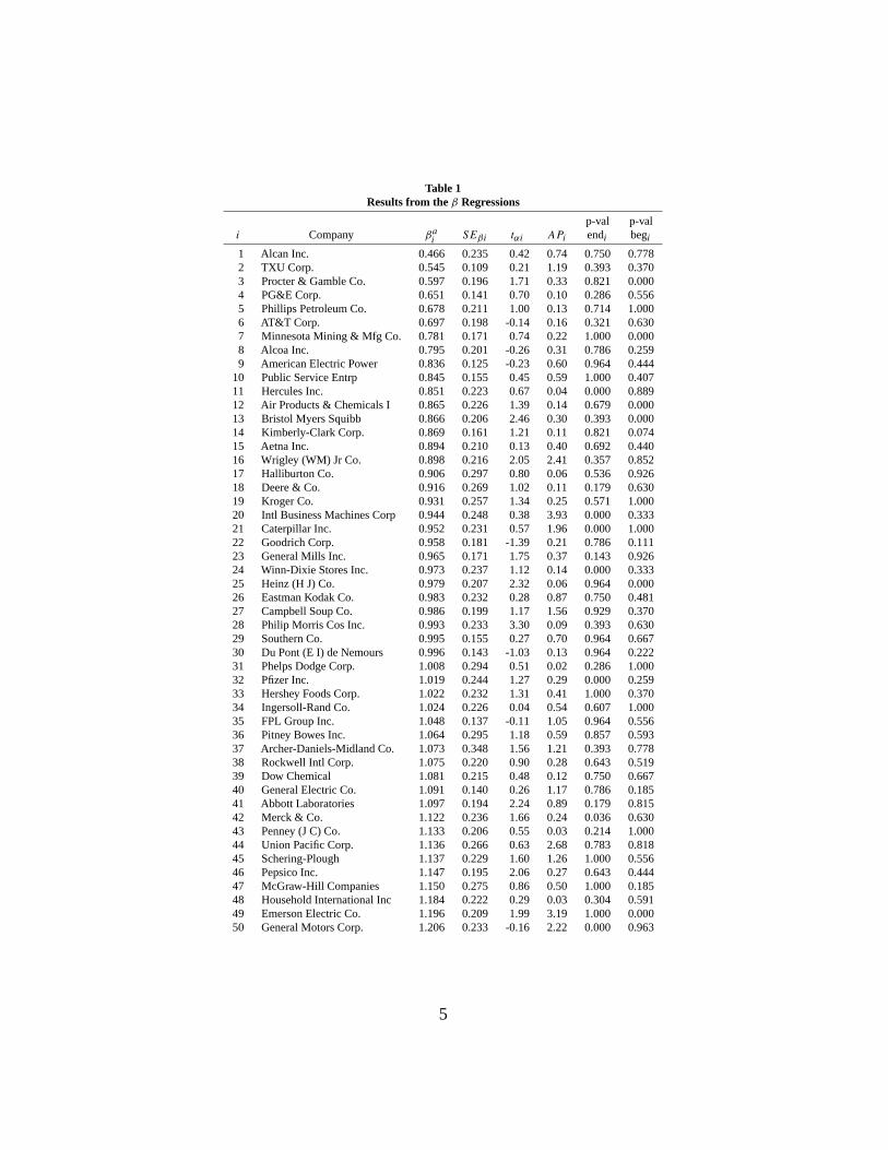
Table 1Results from the β Regressions

p-val p-vali Company βa

iSEβi tαi APi endi begi

1 Alcan Inc. 0.466 0.235 0.42 0.74 0.750 0.7782 TXU Corp. 0.545 0.109 0.21 1.19 0.393 0.3703 Procter & Gamble Co. 0.597 0.196 1.71 0.33 0.821 0.0004 PG&E Corp. 0.651 0.141 0.70 0.10 0.286 0.5565 Phillips Petroleum Co. 0.678 0.211 1.00 0.13 0.714 1.0006 AT&T Corp. 0.697 0.198 -0.14 0.16 0.321 0.6307 Minnesota Mining & Mfg Co. 0.781 0.171 0.74 0.22 1.000 0.0008 Alcoa Inc. 0.795 0.201 -0.26 0.31 0.786 0.2599 American Electric Power 0.836 0.125 -0.23 0.60 0.964 0.444

10 Public Service Entrp 0.845 0.155 0.45 0.59 1.000 0.40711 Hercules Inc. 0.851 0.223 0.67 0.04 0.000 0.88912 Air Products & Chemicals I 0.865 0.226 1.39 0.14 0.679 0.00013 Bristol Myers Squibb 0.866 0.206 2.46 0.30 0.393 0.00014 Kimberly-Clark Corp. 0.869 0.161 1.21 0.11 0.821 0.07415 Aetna Inc. 0.894 0.210 0.13 0.40 0.692 0.44016 Wrigley (WM) Jr Co. 0.898 0.216 2.05 2.41 0.357 0.85217 Halliburton Co. 0.906 0.297 0.80 0.06 0.536 0.92618 Deere & Co. 0.916 0.269 1.02 0.11 0.179 0.63019 Kroger Co. 0.931 0.257 1.34 0.25 0.571 1.00020 Intl Business Machines Corp 0.944 0.248 0.38 3.93 0.000 0.33321 Caterpillar Inc. 0.952 0.231 0.57 1.96 0.000 1.00022 Goodrich Corp. 0.958 0.181 -1.39 0.21 0.786 0.11123 General Mills Inc. 0.965 0.171 1.75 0.37 0.143 0.92624 Winn-Dixie Stores Inc. 0.973 0.237 1.12 0.14 0.000 0.33325 Heinz (H J) Co. 0.979 0.207 2.32 0.06 0.964 0.00026 Eastman Kodak Co. 0.983 0.232 0.28 0.87 0.750 0.48127 Campbell Soup Co. 0.986 0.199 1.17 1.56 0.929 0.37028 Philip Morris Cos Inc. 0.993 0.233 3.30 0.09 0.393 0.63029 Southern Co. 0.995 0.155 0.27 0.70 0.964 0.66730 Du Pont (E I) de Nemours 0.996 0.143 -1.03 0.13 0.964 0.22231 Phelps Dodge Corp. 1.008 0.294 0.51 0.02 0.286 1.00032 Pfizer Inc. 1.019 0.244 1.27 0.29 0.000 0.25933 Hershey Foods Corp. 1.022 0.232 1.31 0.41 1.000 0.37034 Ingersoll-Rand Co. 1.024 0.226 0.04 0.54 0.607 1.00035 FPL Group Inc. 1.048 0.137 -0.11 1.05 0.964 0.55636 Pitney Bowes Inc. 1.064 0.295 1.18 0.59 0.857 0.59337 Archer-Daniels-Midland Co. 1.073 0.348 1.56 1.21 0.393 0.77838 Rockwell Intl Corp. 1.075 0.220 0.90 0.28 0.643 0.51939 Dow Chemical 1.081 0.215 0.48 0.12 0.750 0.66740 General Electric Co. 1.091 0.140 0.26 1.17 0.786 0.18541 Abbott Laboratories 1.097 0.194 2.24 0.89 0.179 0.81542 Merck & Co. 1.122 0.236 1.66 0.24 0.036 0.63043 Penney (J C) Co. 1.133 0.206 0.55 0.03 0.214 1.00044 Union Pacific Corp. 1.136 0.266 0.63 2.68 0.783 0.81845 Schering-Plough 1.137 0.229 1.60 1.26 1.000 0.55646 Pepsico Inc. 1.147 0.195 2.06 0.27 0.643 0.44447 McGraw-Hill Companies 1.150 0.275 0.86 0.50 1.000 0.18548 Household International Inc 1.184 0.222 0.29 0.03 0.304 0.59149 Emerson Electric Co. 1.196 0.209 1.99 3.19 1.000 0.00050 General Motors Corp. 1.206 0.233 -0.16 2.22 0.000 0.963

5

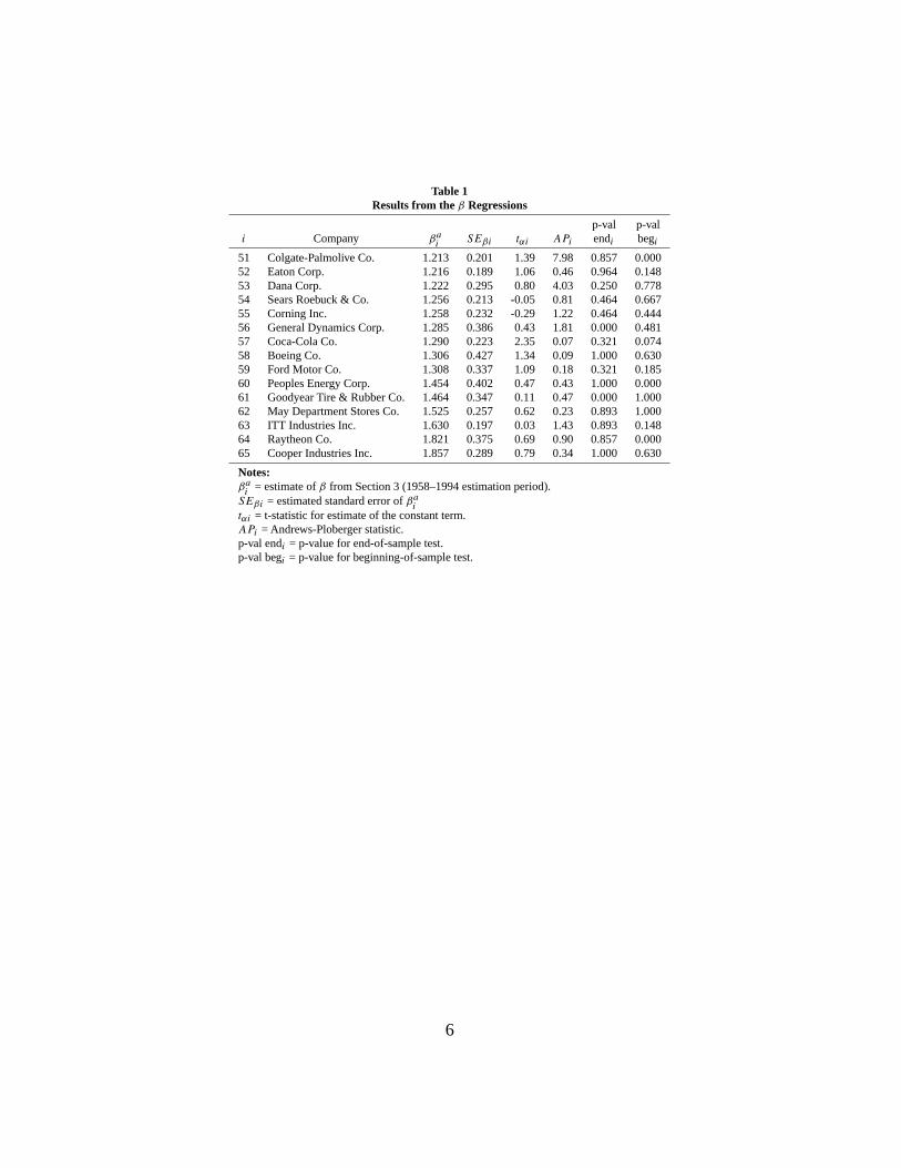
Table 1Results from the β Regressions

p-val p-vali Company βa

iSEβi tαi APi endi begi

51 Colgate-Palmolive Co. 1.213 0.201 1.39 7.98 0.857 0.00052 Eaton Corp. 1.216 0.189 1.06 0.46 0.964 0.14853 Dana Corp. 1.222 0.295 0.80 4.03 0.250 0.77854 Sears Roebuck & Co. 1.256 0.213 -0.05 0.81 0.464 0.66755 Corning Inc. 1.258 0.232 -0.29 1.22 0.464 0.44456 General Dynamics Corp. 1.285 0.386 0.43 1.81 0.000 0.48157 Coca-Cola Co. 1.290 0.223 2.35 0.07 0.321 0.07458 Boeing Co. 1.306 0.427 1.34 0.09 1.000 0.63059 Ford Motor Co. 1.308 0.337 1.09 0.18 0.321 0.18560 Peoples Energy Corp. 1.454 0.402 0.47 0.43 1.000 0.00061 Goodyear Tire & Rubber Co. 1.464 0.347 0.11 0.47 0.000 1.00062 May Department Stores Co. 1.525 0.257 0.62 0.23 0.893 1.00063 ITT Industries Inc. 1.630 0.197 0.03 1.43 0.893 0.14864 Raytheon Co. 1.821 0.375 0.69 0.90 0.857 0.00065 Cooper Industries Inc. 1.857 0.289 0.79 0.34 1.000 0.630

Notes:βai

= estimate ofβ from Section 3 (1958–1994 estimation period).SEβi = estimated standard error ofβa

itαi = t-statistic for estimate of the constant term.APi = Andrews-Ploberger statistic.p-val endi = p-value for end-of-sample test.p-val begi = p-value for beginning-of-sample test.

6

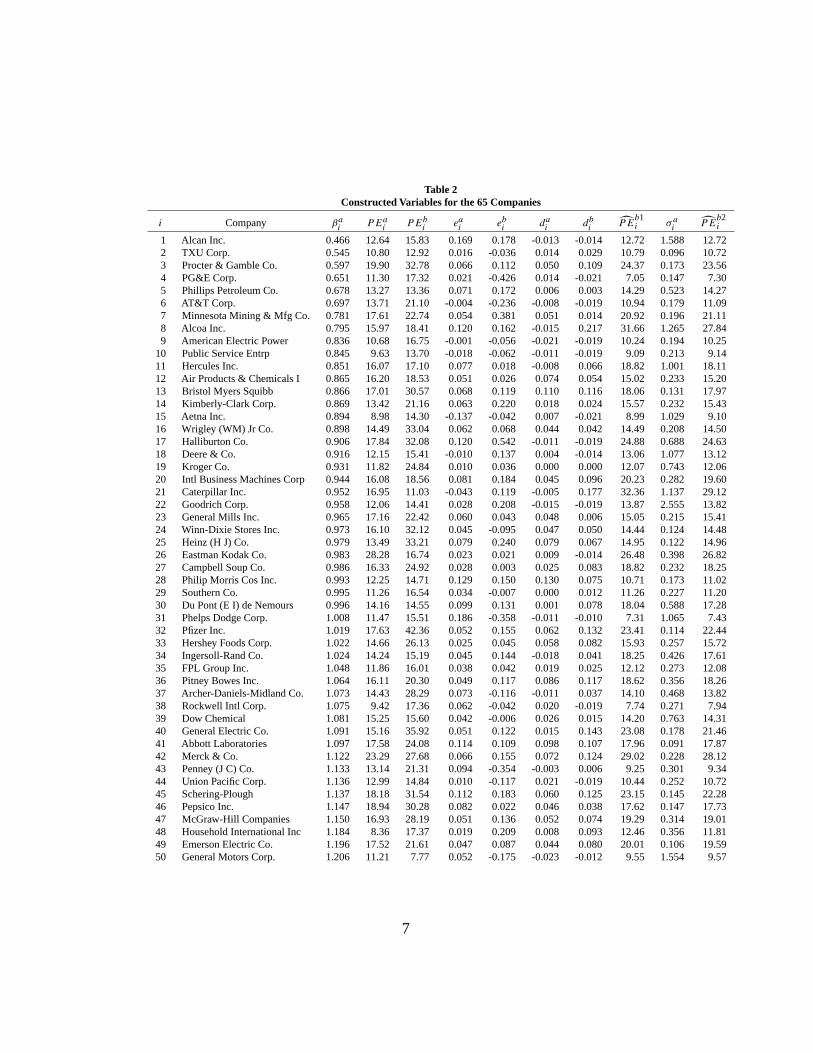
Table 2Constructed Variables for the 65 Companies

i Company βai

PEai

PEbi

eai

ebi

dai

dbi

P̂Eb1i σ a

iP̂E

b2i

1 Alcan Inc. 0.466 12.64 15.83 0.169 0.178 -0.013 -0.014 12.72 1.588 12.722 TXU Corp. 0.545 10.80 12.92 0.016 -0.036 0.014 0.029 10.79 0.096 10.723 Procter & Gamble Co. 0.597 19.90 32.78 0.066 0.112 0.050 0.109 24.37 0.173 23.564 PG&E Corp. 0.651 11.30 17.32 0.021 -0.426 0.014 -0.021 7.05 0.147 7.305 Phillips Petroleum Co. 0.678 13.27 13.36 0.071 0.172 0.006 0.003 14.29 0.523 14.276 AT&T Corp. 0.697 13.71 21.10 -0.004 -0.236 -0.008 -0.019 10.94 0.179 11.097 Minnesota Mining & Mfg Co. 0.781 17.61 22.74 0.054 0.381 0.051 0.014 20.92 0.196 21.118 Alcoa Inc. 0.795 15.97 18.41 0.120 0.162 -0.015 0.217 31.66 1.265 27.849 American Electric Power 0.836 10.68 16.75 -0.001 -0.056 -0.021 -0.019 10.24 0.194 10.25

10 Public Service Entrp 0.845 9.63 13.70 -0.018 -0.062 -0.011 -0.019 9.09 0.213 9.1411 Hercules Inc. 0.851 16.07 17.10 0.077 0.018 -0.008 0.066 18.82 1.001 18.1112 Air Products & Chemicals I 0.865 16.20 18.53 0.051 0.026 0.074 0.054 15.02 0.233 15.2013 Bristol Myers Squibb 0.866 17.01 30.57 0.068 0.119 0.110 0.116 18.06 0.131 17.9714 Kimberly-Clark Corp. 0.869 13.42 21.16 0.063 0.220 0.018 0.024 15.57 0.232 15.4315 Aetna Inc. 0.894 8.98 14.30 -0.137 -0.042 0.007 -0.021 8.99 1.029 9.1016 Wrigley (WM) Jr Co. 0.898 14.49 33.04 0.062 0.068 0.044 0.042 14.49 0.208 14.5017 Halliburton Co. 0.906 17.84 32.08 0.120 0.542 -0.011 -0.019 24.88 0.688 24.6318 Deere & Co. 0.916 12.15 15.41 -0.010 0.137 0.004 -0.014 13.06 1.077 13.1219 Kroger Co. 0.931 11.82 24.84 0.010 0.036 0.000 0.000 12.07 0.743 12.0620 Intl Business Machines Corp 0.944 16.08 18.56 0.081 0.184 0.045 0.096 20.23 0.282 19.6021 Caterpillar Inc. 0.952 16.95 11.03 -0.043 0.119 -0.005 0.177 32.36 1.137 29.1222 Goodrich Corp. 0.958 12.06 14.41 0.028 0.208 -0.015 -0.019 13.87 2.555 13.8223 General Mills Inc. 0.965 17.16 22.42 0.060 0.043 0.048 0.006 15.05 0.215 15.4124 Winn-Dixie Stores Inc. 0.973 16.10 32.12 0.045 -0.095 0.047 0.050 14.44 0.124 14.4825 Heinz (H J) Co. 0.979 13.49 33.21 0.079 0.240 0.079 0.067 14.95 0.122 14.9626 Eastman Kodak Co. 0.983 28.28 16.74 0.023 0.021 0.009 -0.014 26.48 0.398 26.8227 Campbell Soup Co. 0.986 16.33 24.92 0.028 0.003 0.025 0.083 18.82 0.232 18.2528 Philip Morris Cos Inc. 0.993 12.25 14.71 0.129 0.150 0.130 0.075 10.71 0.173 11.0229 Southern Co. 0.995 11.26 16.54 0.034 -0.007 0.000 0.012 11.26 0.227 11.2030 Du Pont (E I) de Nemours 0.996 14.16 14.55 0.099 0.131 0.001 0.078 18.04 0.588 17.2831 Phelps Dodge Corp. 1.008 11.47 15.51 0.186 -0.358 -0.011 -0.010 7.31 1.065 7.4332 Pfizer Inc. 1.019 17.63 42.36 0.052 0.155 0.062 0.132 23.41 0.114 22.4433 Hershey Foods Corp. 1.022 14.66 26.13 0.025 0.045 0.058 0.082 15.93 0.257 15.7234 Ingersoll-Rand Co. 1.024 14.24 15.19 0.045 0.144 -0.018 0.041 18.25 0.426 17.6135 FPL Group Inc. 1.048 11.86 16.01 0.038 0.042 0.019 0.025 12.12 0.273 12.0836 Pitney Bowes Inc. 1.064 16.11 20.30 0.049 0.117 0.086 0.117 18.62 0.356 18.2637 Archer-Daniels-Midland Co. 1.073 14.43 28.29 0.073 -0.116 -0.011 0.037 14.10 0.468 13.8238 Rockwell Intl Corp. 1.075 9.42 17.36 0.062 -0.042 0.020 -0.019 7.74 0.271 7.9439 Dow Chemical 1.081 15.25 15.60 0.042 -0.006 0.026 0.015 14.20 0.763 14.3140 General Electric Co. 1.091 15.16 35.92 0.051 0.122 0.015 0.143 23.08 0.178 21.4641 Abbott Laboratories 1.097 17.58 24.08 0.114 0.109 0.098 0.107 17.96 0.091 17.8742 Merck & Co. 1.122 23.29 27.68 0.066 0.155 0.072 0.124 29.02 0.228 28.1243 Penney (J C) Co. 1.133 13.14 21.31 0.094 -0.354 -0.003 0.006 9.25 0.301 9.3444 Union Pacific Corp. 1.136 12.99 14.84 0.010 -0.117 0.021 -0.019 10.44 0.252 10.7245 Schering-Plough 1.137 18.18 31.54 0.112 0.183 0.060 0.125 23.15 0.145 22.2846 Pepsico Inc. 1.147 18.94 30.28 0.082 0.022 0.046 0.038 17.62 0.147 17.7347 McGraw-Hill Companies 1.150 16.93 28.19 0.051 0.136 0.052 0.074 19.29 0.314 19.0148 Household International Inc 1.184 8.36 17.37 0.019 0.209 0.008 0.093 12.46 0.356 11.8149 Emerson Electric Co. 1.196 17.52 21.61 0.047 0.087 0.044 0.080 20.01 0.106 19.5950 General Motors Corp. 1.206 11.21 7.77 0.052 -0.175 -0.023 -0.012 9.55 1.554 9.57

7

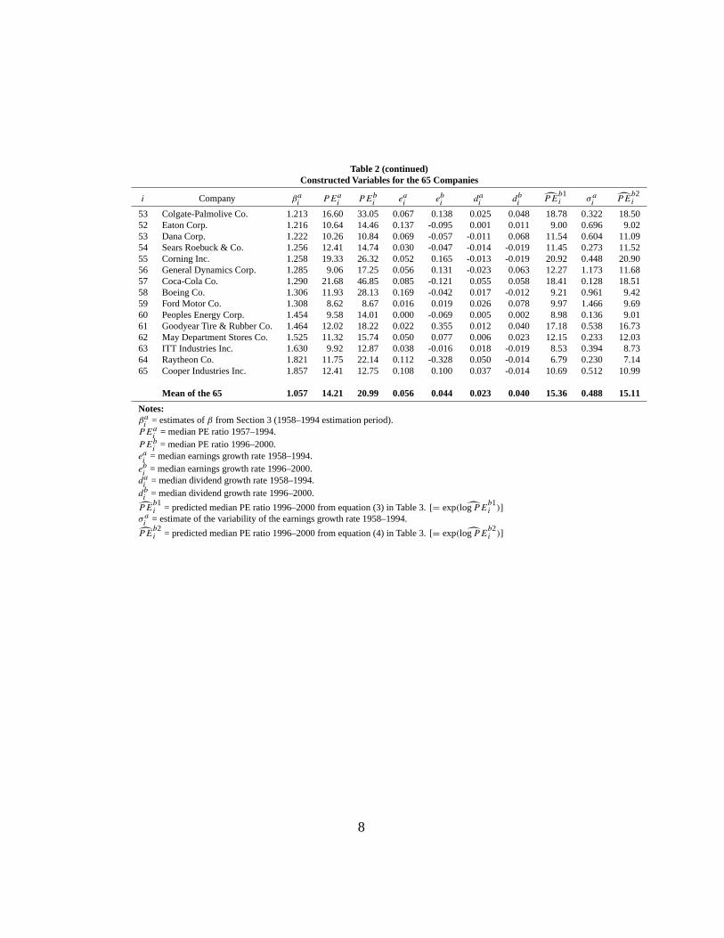
Table 2 (continued)Constructed Variables for the 65 Companies

i Company βai

PEai

PEbi

eai

ebi

dai

dbi

P̂Eb1i σ a

iP̂E

b2i

53 Colgate-Palmolive Co. 1.213 16.60 33.05 0.067 0.138 0.025 0.048 18.78 0.322 18.5052 Eaton Corp. 1.216 10.64 14.46 0.137 -0.095 0.001 0.011 9.00 0.696 9.0253 Dana Corp. 1.222 10.26 10.84 0.069 -0.057 -0.011 0.068 11.54 0.604 11.0954 Sears Roebuck & Co. 1.256 12.41 14.74 0.030 -0.047 -0.014 -0.019 11.45 0.273 11.5255 Corning Inc. 1.258 19.33 26.32 0.052 0.165 -0.013 -0.019 20.92 0.448 20.9056 General Dynamics Corp. 1.285 9.06 17.25 0.056 0.131 -0.023 0.063 12.27 1.173 11.6857 Coca-Cola Co. 1.290 21.68 46.85 0.085 -0.121 0.055 0.058 18.41 0.128 18.5158 Boeing Co. 1.306 11.93 28.13 0.169 -0.042 0.017 -0.012 9.21 0.961 9.4259 Ford Motor Co. 1.308 8.62 8.67 0.016 0.019 0.026 0.078 9.97 1.466 9.6960 Peoples Energy Corp. 1.454 9.58 14.01 0.000 -0.069 0.005 0.002 8.98 0.136 9.0161 Goodyear Tire & Rubber Co. 1.464 12.02 18.22 0.022 0.355 0.012 0.040 17.18 0.538 16.7362 May Department Stores Co. 1.525 11.32 15.74 0.050 0.077 0.006 0.023 12.15 0.233 12.0363 ITT Industries Inc. 1.630 9.92 12.87 0.038 -0.016 0.018 -0.019 8.53 0.394 8.7364 Raytheon Co. 1.821 11.75 22.14 0.112 -0.328 0.050 -0.014 6.79 0.230 7.1465 Cooper Industries Inc. 1.857 12.41 12.75 0.108 0.100 0.037 -0.014 10.69 0.512 10.99

Mean of the 65 1.057 14.21 20.99 0.056 0.044 0.023 0.040 15.36 0.488 15.11

Notes:βai

= estimates ofβ from Section 3 (1958–1994 estimation period).PEa

i= median PE ratio 1957–1994.

PEbi

= median PE ratio 1996–2000.eai

= median earnings growth rate 1958–1994.ebi

= median earnings growth rate 1996–2000.dai

= median dividend growth rate 1958–1994.dbi

= median dividend growth rate 1996–2000.

P̂Eb1i = predicted median PE ratio 1996–2000 from equation (3) in Table 3. [= exp( ̂logPE

b1i )]

σai

= estimate of the variability of the earnings growth rate 1958–1994.

P̂Eb2i = predicted median PE ratio 1996–2000 from equation (4) in Table 3. [= exp( ̂logPE

b2i )]

8

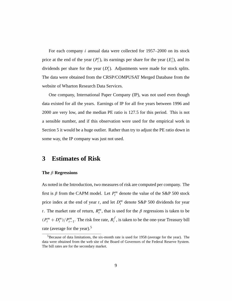
For each companyi annual data were collected for 1957–2000 on its stock

price at the end of the year (P it ), its earnings per share for the year (Ei

t ), and its

dividends per share for the year (Dit ). Adjustments were made for stock splits.

The data were obtained from the CRSP/COMPUSAT Merged Database from the

website of Wharton Research Data Services.

One company, International Paper Company (IP), was not used even though

data existed for all the years. Earnings of IP for all five years between 1996 and

2000 are very low, and the median PE ratio is 127.5 for this period. This is not

a sensible number, and if this observation were used for the empirical work in

Section 5 it would be a huge outlier. Rather than try to adjust the PE ratio down in

some way, the IP company was just not used.

3 Estimates of Risk

The β Regressions

As noted in the Introduction, two measures of risk are computed per company. The

first is β from the CAPM model. LetP mt denote the value of the S&P 500 stock

price index at the end of yeart , and letDmt denote S&P 500 dividends for year

t . The market rate of return,Rmt , that is used for theβ regressions is taken to be

(P mt + Dm

t )/P mt−1. The risk free rate,Rf

t , is taken to be the one-year Treasury bill

rate (average for the year).5

5Because of data limitations, the six-month rate is used for 1958 (average for the year). Thedata were obtained from the web site of the Board of Governors of the Federal Reserve System.The bill rates are for the secondary market.

9

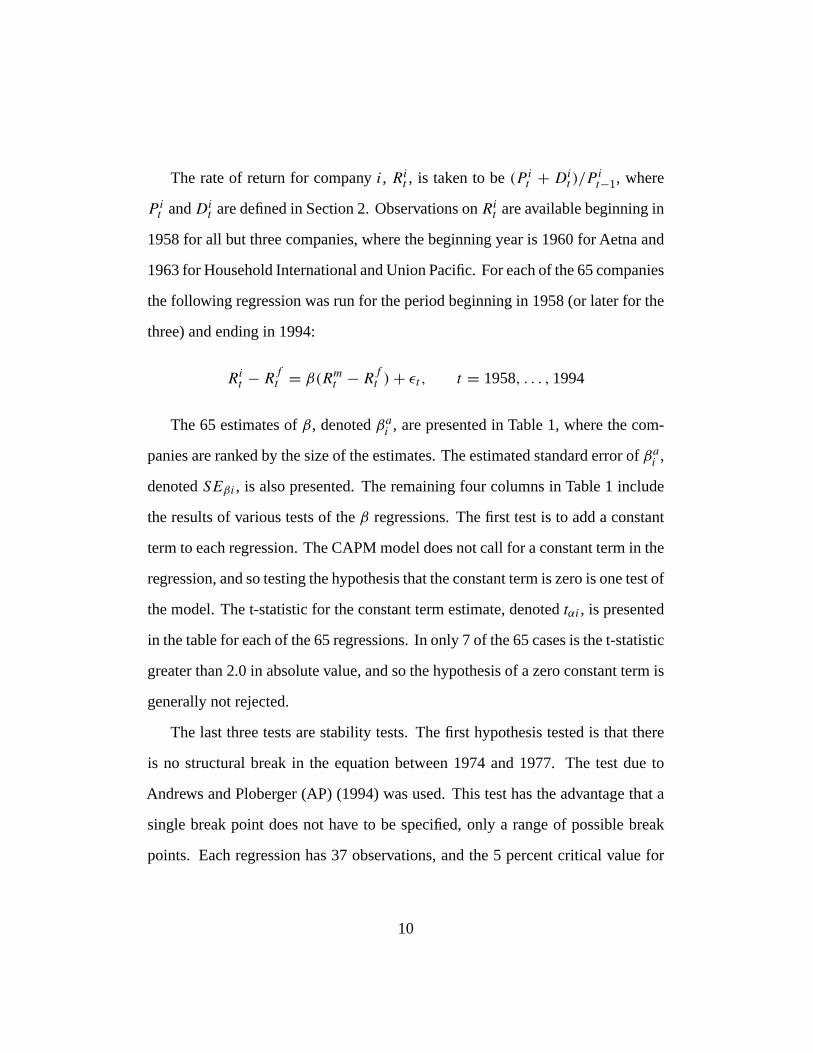
The rate of return for companyi, Rit , is taken to be(P i

t + Dit )/P

it−1, where

P it andDi

t are defined in Section 2. Observations onRit are available beginning in

1958 for all but three companies, where the beginning year is 1960 for Aetna and

1963 for Household International and Union Pacific. For each of the 65 companies

the following regression was run for the period beginning in 1958 (or later for the

three) and ending in 1994:

Rit − R

ft = β(Rm

t − Rft ) + εt , t = 1958, . . . , 1994

The 65 estimates ofβ, denotedβai , are presented in Table 1, where the com-

panies are ranked by the size of the estimates. The estimated standard error ofβai ,

denotedSEβi , is also presented. The remaining four columns in Table 1 include

the results of various tests of theβ regressions. The first test is to add a constant

term to each regression. The CAPM model does not call for a constant term in the

regression, and so testing the hypothesis that the constant term is zero is one test of

the model. The t-statistic for the constant term estimate, denotedtαi , is presented

in the table for each of the 65 regressions. In only 7 of the 65 cases is the t-statistic

greater than 2.0 in absolute value, and so the hypothesis of a zero constant term is

generally not rejected.

The last three tests are stability tests. The first hypothesis tested is that there

is no structural break in the equation between 1974 and 1977. The test due to

Andrews and Ploberger (AP) (1994) was used. This test has the advantage that a

single break point does not have to be specified, only a range of possible break

points. Each regression has 37 observations, and the 5 percent critical value for

10

the AP statistic for this number of observations and one coefficient is 2.00.6 In

Table 1 only 7 of the 65 values ofAPi are greater than 2.00, and so the stability

hypothesis is generally not rejected.

The next test is of the hypothesis that there is no structural break near the end

of the sample period—in 1990. The test due to Andrews (2002) was used. The

p-values from this test are presented in the table. Only 9 of the 65 p-values are less

than .05, and so the end-of-sample stability hypothesis is generally not rejected.

The final test is of the hypothesis that there is no structural break near the

beginning of the sample period—in 1963.7 The Andrews (2002) test was also used

for this purpose. The p-values from this test are presented in the table. Again,

only 9 of the 65 p-values are less than .05, and so the beginning-of-sample stability

hypothesis is generally not rejected.

The overall results are thus fairly supportive of the CAPM model for this set

of companies. The regressions are mostly stable, and most of the estimates of

the constant term are not significant. On the negative side, most of the estimates

of β are not significantly different from 1.0, which means that there is not much

precision in the ranking of theβ estimates. It will be seen in Section 5, however,

that there is some evidence that the estimates ofβ are picking up risk differences

across companies.

6See Andrews and Ploberger (1994), Table I.7For Aetna the year was 1965, and for Household International and Union Pacific the year was

1968.

11

Variation of Earnings

Another measure of the risk of a company, not consistent with the CAPM model, is

the variation of its earnings. Maybe the average investor looks only at a company’s

earnings fluctuations in judging how risky it is? The measure that was used is as

follows. In the next section the growth rates of each company’s real earnings

are computed for 1958–1994.8 These growth rates are ranked, and the median,

denotedeai , is computed. The variation in the growth rate of earnings, denoted

σai , is then taken from this ranking to be the difference between the value above

which 20 percent of the growth rates lie and the value below which 20 percent of

the growth rates lie. This range was used as the measure of variation because it is

not sensible to compute variances in the usual way due to extreme values at both

ends of the ranking. The values ofσai are presented in the second-to-last column

of Table 2.

4 Computing PE Ratios, Earnings Growth, andDividend Growth

Computing average PE ratios is problematic because earnings can be very small or

negative. For the present calculations the PE ratio for a given year was taken to be

large (and positive) if earnings for the year were negative. The ratio was taken to

be large enough to put the observation at the top when the observations are ranked.

The average PE ratio was then taken to be the median of the ranked observations.

This way of treating negative earnings affects the calculation of the average value

8In some cases the first year was later than 1958.

12

only in that the large values are put at the top before the median is taken.

For each company the median was computed for the 1957–1994 period. For

a few companies the earnings data began after 1957, and for these companies the

median was computed for the period consisting of the first available observation

through 1994. The median for companyi for this period will be denotedPEai ,

wherea denotes the 1957–1994 (or slightly shorter) period.

The median for each company was also computed for the 1996–2000 period,

which meant ranking the five yearly observations and taking the third one. For one

company, Corning, three of the five PE ratios were very large because of very low

earnings, and for Corning the average PE ratio was taken to be the second lowest

rather than the third. The median for companyi for this period will be denoted

PEbi , whereb denotes the 1996–2000 period. BothPEa

i andPEbi are presented

in Table 2.

The last row in Table 2 presents the mean of the 65 observations for each

variable. The mean ofPEai is 14.21, and the mean ofPEb

i is 20.99. There has

thus been on average a large increase in the median PE ratio from before to after

1995 for these companies, which is consistent with the S&P 500 data discussed in

Section 1.

Four other variables per company were also computed: the median growth

rates of earnings for the two periods, denotedeai andeb

i , and the median growth

rates of dividends for the two periods, denoteddei anddb

i . Earnings and dividends

from Section 2 were first deflated by the GDP deflator:ERit = Ei

t /GDPDt and

DRit = Di

t /GDPDt , whereGDPDt is the GDP deflator for yeart , ER denotes

real earnings, andDR denotes real dividends. The growth rate of real earnings was

13

then computed as(ERit −ERi

t−1)/ERit−1 whenERi

t−1 was positive. WhenERit−1

was zero or negative, the growth rate was taken to be a large positive number if

ERit > ERi

t−1 and a large negative number ifERit < ERi

t−1. For each period the

growth rates were ranked and the median of the ranked observations was taken.9

(As discussed in the previous section, these growth rates of real earnings for 1958–

1994 were used to computeσai , the variability measure.) The same procedure was

followed for dividends, where there are zero values for a few of theDit but no

negative values. Again, medians were computed for the period up to 1994 and for

the period 1996–2000. The four median growth rates per company are presented

in Table 2.

It can be seen from the last row in Table 2 that on average earnings growth was

less after 1995 (mean of .044 versus .056) and dividend growth was greater (mean

of .040 versus .023).

5 The Cross Company Regressions

1957–1994 Period

If 1957–1994 was a period in which there were no large shifts in the risk charac-

teristics of the 65 companies, then the estimates ofβai or σa

i may be reasonable

approximations of the riskiness of the companies. One would expect, other things

being equal, for more risky companies to have on average lower PE ratios. If,

9For the second period, which consists of only five observations, this procedure did not result insensible growth rates for five companies (Boeing, Goodyear, Halliburton, ITT, and Phillips). Foreach of these five companies total real earnings were computed for 1990–1994 and 1996–2000,and the growth rate (at an annual rate) between these two periods was used foreb

i .

14

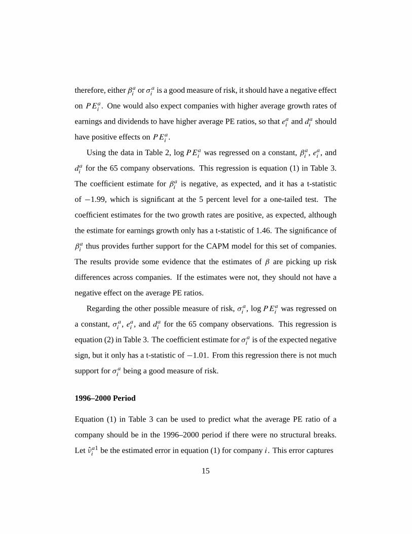
therefore, eitherβai orσa

i is a good measure of risk, it should have a negative effect

on PEai . One would also expect companies with higher average growth rates of

earnings and dividends to have higher average PE ratios, so thateai andda

i should

have positive effects onPEai .

Using the data in Table 2, logPEai was regressed on a constant,βa

i , eai , and

dai for the 65 company observations. This regression is equation (1) in Table 3.

The coefficient estimate forβai is negative, as expected, and it has a t-statistic

of −1.99, which is significant at the 5 percent level for a one-tailed test. The

coefficient estimates for the two growth rates are positive, as expected, although

the estimate for earnings growth only has a t-statistic of 1.46. The significance of

βai thus provides further support for the CAPM model for this set of companies.

The results provide some evidence that the estimates ofβ are picking up risk

differences across companies. If the estimates were not, they should not have a

negative effect on the average PE ratios.

Regarding the other possible measure of risk,σai , logPEa

i was regressed on

a constant,σai , ea

i , anddai for the 65 company observations. This regression is

equation (2) in Table 3. The coefficient estimate forσai is of the expected negative

sign, but it only has a t-statistic of−1.01. From this regression there is not much

support forσai being a good measure of risk.

1996–2000 Period

Equation (1) in Table 3 can be used to predict what the average PE ratio of a

company should be in the 1996–2000 period if there were no structural breaks.

Let ν̂a1i be the estimated error in equation (1) for companyi. This error captures

15

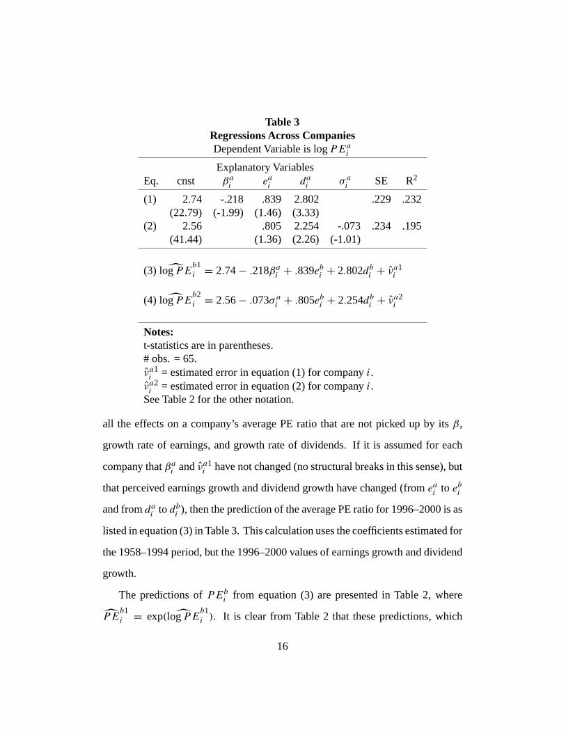
Table 3Regressions Across CompaniesDependent Variable is logPEa

i

Explanatory VariablesEq. cnst βa

i eai da

i σ ai SE R2

(1) 2.74 -.218 .839 2.802 .229 .232(22.79) (-1.99) (1.46) (3.33)

(2) 2.56 .805 2.254 -.073 .234 .195(41.44) (1.36) (2.26) (-1.01)

(3) ̂logPEb1i = 2.74− .218βa

i + .839ebi + 2.802db

i + ν̂a1i

(4) ̂logPEb2i = 2.56− .073σa

i + .805ebi + 2.254db

i + ν̂a2i

Notes:t-statistics are in parentheses.# obs. = 65.ν̂a1i = estimated error in equation (1) for companyi.

ν̂a2i = estimated error in equation (2) for companyi.

See Table 2 for the other notation.

all the effects on a company’s average PE ratio that are not picked up by itsβ,

growth rate of earnings, and growth rate of dividends. If it is assumed for each

company thatβai andν̂a1

i have not changed (no structural breaks in this sense), but

that perceived earnings growth and dividend growth have changed (fromeai to eb

i

and fromdai to db

i ), then the prediction of the average PE ratio for 1996–2000 is as

listed in equation (3) in Table 3. This calculation uses the coefficients estimated for

the 1958–1994 period, but the 1996–2000 values of earnings growth and dividend

growth.

The predictions ofPEbi from equation (3) are presented in Table 2, where

P̂Eb1i = exp( ̂logPE

b1i ). It is clear from Table 2 that these predictions, which

16

are the predicted average PE ratios for 1996–2000, are close to the actual average

PE ratios for 1957–1994. Becauseβai andν̂a1

i are used in equation (3), the only

reason logPEai and ̂logPE

b1i differ for a given company is because the growth

rates of earnings and dividends differ between the two periods. The net effect of

these differences is in general not large, i.e., logPEai and ̂logPE

b1i are in general

close.

Note that theβs have not been reestimated for the predictions:βai is used in

equation (3). It would not have been practical to reestimate theβs because five

observations per company is not enough to get trustworthy estimates. More to

the point, however, as discussed above, the analysis in this paper is based on the

assumption that the risk characteristics of the companies have not changed, i.e.,

that a company’sβ has not changed.

Equation (2) in Table 3 can also be used to predict what the average PE ratio of

a company should be in the 1996–2000 period if there were no structural breaks.

This is done in equation (4), whereν̂a2i is the estimated error in equation (2) for

companyi. This prediction, of course, uses as the measure of riskσai instead of

βai . The predictions ofPEb

i from equation (4) are also presented in Table 2, where

it is again clear that these predictions are close to the actual average PE ratios for

1957–1994.

The main interest of this paper is to examine the difference between the actual

average PE ratio for 1996–2000 (PEbi ) and the predicted average under the as-

sumption of no structural changes (̂PEb1i or P̂E

b2i ). Table 2 shows that on average

this difference is large and positive. Now, if the increase in the average PE ratios

is due to a fall in investors’ risk aversion, more risky companies should have had

17

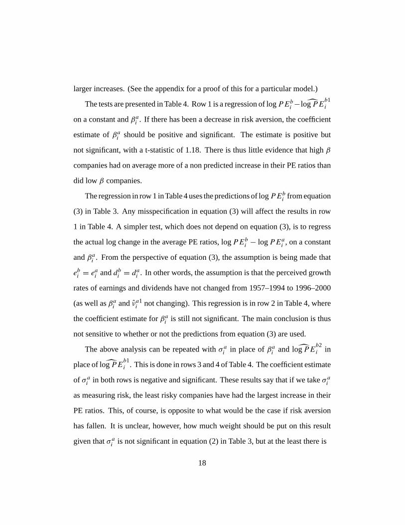
larger increases. (See the appendix for a proof of this for a particular model.)

The tests are presented in Table 4. Row 1 is a regression of logPEbi − ̂logPE

b1i

on a constant andβai . If there has been a decrease in risk aversion, the coefficient

estimate ofβai should be positive and significant. The estimate is positive but

not significant, with a t-statistic of 1.18. There is thus little evidence that highβ

companies had on average more of a non predicted increase in their PE ratios than

did low β companies.

The regression in row 1 inTable 4 uses the predictions of logPEbi from equation

(3) in Table 3. Any misspecification in equation (3) will affect the results in row

1 in Table 4. A simpler test, which does not depend on equation (3), is to regress

the actual log change in the average PE ratios, logPEbi − logPEa

i , on a constant

andβai . From the perspective of equation (3), the assumption is being made that

ebi = ea

i anddbi = da

i . In other words, the assumption is that the perceived growth

rates of earnings and dividends have not changed from 1957–1994 to 1996–2000

(as well asβai andν̂a1

i not changing). This regression is in row 2 in Table 4, where

the coefficient estimate forβai is still not significant. The main conclusion is thus

not sensitive to whether or not the predictions from equation (3) are used.

The above analysis can be repeated withσai in place ofβa

i and ̂logPEb2i in

place of ̂logPEb1i . This is done in rows 3 and 4 of Table 4. The coefficient estimate

of σai in both rows is negative and significant. These results say that if we takeσa

i

as measuring risk, the least risky companies have had the largest increase in their

PE ratios. This, of course, is opposite to what would be the case if risk aversion

has fallen. It is unclear, however, how much weight should be put on this result

given thatσai is not significant in equation (2) in Table 3, but at the least there is

18

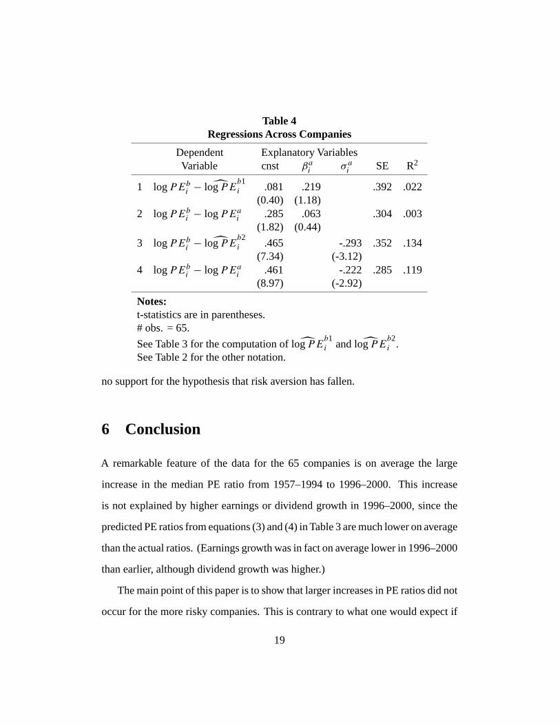
Table 4Regressions Across Companies

Dependent Explanatory VariablesVariable cnst βa

i σ ai SE R2

1 logPEbi − ̂logPE

b1i .081 .219 .392 .022

(0.40) (1.18)2 logPEb

i − logPEai .285 .063 .304 .003

(1.82) (0.44)

3 logPEbi − ̂logPE

b2i .465 -.293 .352 .134

(7.34) (-3.12)4 logPEb

i − logPEai .461 -.222 .285 .119

(8.97) (-2.92)

Notes:t-statistics are in parentheses.# obs. = 65.

See Table 3 for the computation of̂logPEb1i and ̂logPE

b2i .

See Table 2 for the other notation.

no support for the hypothesis that risk aversion has fallen.

6 Conclusion

A remarkable feature of the data for the 65 companies is on average the large

increase in the median PE ratio from 1957–1994 to 1996–2000. This increase

is not explained by higher earnings or dividend growth in 1996–2000, since the

predicted PE ratios from equations (3) and (4) in Table 3 are much lower on average

than the actual ratios. (Earnings growth was in fact on average lower in 1996–2000

than earlier, although dividend growth was higher.)

The main point of this paper is to show that larger increases in PE ratios did not

occur for the more risky companies. This is contrary to what one would expect if

19

there were a fall in the degree of risk aversion of the average investor after 1995.

Some other explanation is needed for the large average PE increases.

The results in this paper may have implications for the future growth of stock

prices. Since the degree of risk aversion does not appear to have fallen, the reason

for the large PE increases may be due to something less fundamental and permanent.

If, for example, they have been due to unrealistically large expectations of future

earnings or dividends, the PE increases are less likely to last than if they have been

due to a fall in risk aversion.

20

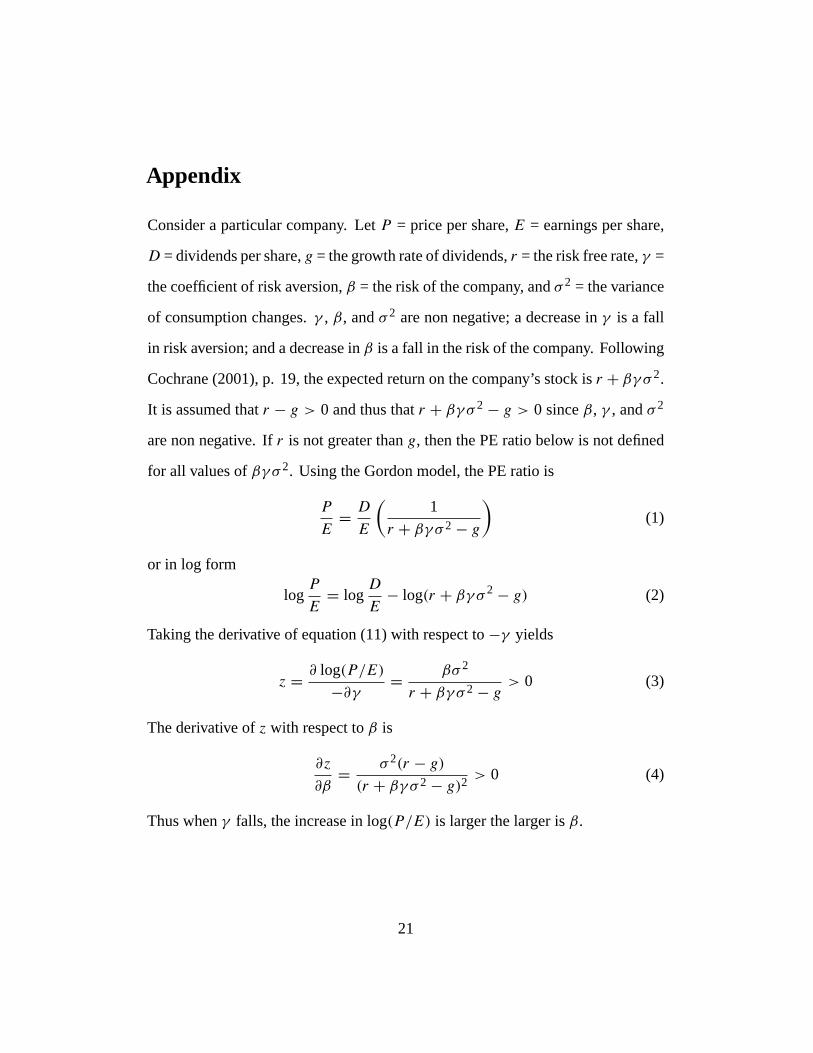
Appendix

Consider a particular company. LetP = price per share,E = earnings per share,

D = dividends per share,g = the growth rate of dividends,r = the risk free rate,γ =

the coefficient of risk aversion,β = the risk of the company, andσ 2 = the variance

of consumption changes.γ , β, andσ 2 are non negative; a decrease inγ is a fall

in risk aversion; and a decrease inβ is a fall in the risk of the company. Following

Cochrane (2001), p. 19, the expected return on the company’s stock isr + βγσ 2.

It is assumed thatr − g > 0 and thus thatr + βγσ 2 − g > 0 sinceβ, γ , andσ 2

are non negative. Ifr is not greater thang, then the PE ratio below is not defined

for all values ofβγσ 2. Using the Gordon model, the PE ratio is

P

E= D

E

(1

r + βγσ 2 − g

)(1)

or in log form

logP

E= log

D

E− log(r + βγσ 2 − g) (2)

Taking the derivative of equation (11) with respect to−γ yields

z = ∂ log(P/E)

−∂γ= βσ 2

r + βγσ 2 − g> 0 (3)

The derivative ofz with respect toβ is

∂z

∂β= σ 2(r − g)

(r + βγσ 2 − g)2> 0 (4)

Thus whenγ falls, the increase in log(P/E) is larger the larger isβ.

21

References

[1] Andrews, Donald W.K., 2002, “End-of-Sample Instability Tests,” CowlesFoundation Discussion Paper No. 1369, May.

[2] Andrews, Donald W.K., and W. Ploberger, 1994, “Optimal Tests When aNuisance Parameter is Present Only Under the Alternative,”Econometrica,62,

[3] Campbell, John Y., and John H. Cochrane, 1999, “By Force of Habit: AConsumption-Based Explanation of Aggregate Stock Market Behavior,”Journal of Political Economy, 107, 205-251.

[4] Cochrane, John, H., 2001,Asset Pricing, Princeton: Princeton UniversityPress.

[5] Glassman, James K., and Kevin A. Hassett, 1999,DOW 36,000, New York:Three Rivers Press.

[6] Jagannathan, Ravi, Ellen R. McGrattan, and Anna Scherbina, 2000, “TheDeclining U.S. Equity Premium,”Federal Reserve Bank of MinneapolisQuarterly Review, 24 (Fall), 3-19.

[7] Kocherlakota, Narayana R., 1996, “The Equity Premium: It’s Still a Puzzle,”Journal of Economic Literature, 34 (March), 42-71.

[8] Shiller, Robert J., 2000,Irrational Exuberance, Princeton, New Jersey:Princeton University Press.

[9] Siegel, Jeremy J., 1999, “The Shrinking Equity Premium: Historical Factsand Future Forecasts,”Journal of Portfolio Management, 26 (Fall), 10-17.

[10] Siegel, Jeremy J., and Richard H. Thaler, 1997, “The Equity Premium Puz-zle,” Journal of Economic Perspectives, 11 (Winter), 191-200.

[11] Welch, Ivo, 2000, “Views of Financial Economists on the Equity Premiumand on Professional Controversies,”Journal of Business, 73 (October), 501-537.

22