COVID-induced sovereign risk in the euro area:

When did the ECB stop the spread?

Aymeric Ortmans∗ Fabien Tripier†

March 11, 2021

(preliminary version, please do not circulate)

Abstract

This paper studies how the announcement of ECB’s monetary policies has stopped the spread of the COVID-

19 pandemic through the European sovereign debt market. We show that up to March 9, the occurrence of

new cases in euro area countries has a sizeable and persistent effect on 10-year sovereign bond spreads relative

to Germany: 10 new confirmed cases per million people is accompanied by an immediate increase in the

spread of 0.03 percentage point (ppt) which lasts 5 days after, reaching an increase of 0.35 ppt. Afterwards,

the effect is close to zero and not significant. We interpret this change as a successful outcome of the ECB’s

press conference on March 12 despite the ”we are not here to close spreads” controversy. Our results hold for

the stock market, giving further evidence of the effectiveness of March 12 ECB’s announcements in stopping

the financial turmoil. A counterfactual analysis shows that without the shift in the sensitivity of sovereign

bond markets to COVID-19, spreads would have surged to 4.3% in France, 12.7% in Spain, and 20.0% in

Italy as early as March 18, when the ECB’s Pandemic Emergency Purchase Programme has finally been

announced.

Keywords: COVID-19; European Central Bank; Sovereign debt; Monetary policy; Local projections

JEL Codes: E52, E58, E65, H63

∗Universite Paris-Saclay, Univ Evry, EPEE, 91025, Evry-Courcouronnes, France. aymeric.ortmans@univ-evry.fr

†Universite Paris-Saclay, Univ Evry, EPEE, 91025, Evry-Courcouronnes, France & CEPII. fabien.tripier@univ-evry.fr

”I can assure you on that page that first of all we will make use of all the flexibilities that are

embedded in the framework of the asset purchase programme, [...] but we are not here to close

spreads.” Christine Lagarde, President of the ECB, Press conference, 12 March 2020.

”The ECB will ensure that all sectors of the economy can benefit from supportive financing con-

ditions that enable them to absorb this shock. This applies equally to families, firms, banks and

governments.” ECB Governing Council Press release, 18 March 2020.

1 Introduction

The COVID-19 virus pandemic started on December 31, 2019 in China and hit Europe almost one month

later, according to the World Health Organization (WHO).1 As a serious threat to the economy, the rapid

spread of the virus led to a sizeable financial turmoil in Europe. The downturn was particularly strong in Italy,

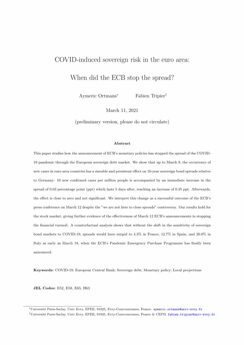
the most affected country in Europe, where the interest rate spread vis-a-vis Germany sharply rose from 1.4

to 2.5% and the stock market considerably fell by 40% between February 19 and March 12 (Figure 1). On

March 12, the ECB announced a set of monetary policy measures to support the economy in the face of the

pandemic. The announcement of these measures gave rise to controversy over President Christine Lagarde’s

announcement that the ECB would certainly use ”all the flexibilities that are embedded in the framework of

the asset purchase programme”, but also that ”[they] are not here to close spreads”. This last sentence has

been widely commentated as a communication failure, contrasting with the famous ”Whatever it takes” of her

predecessor Mario Draghi.2 After a crash on March 12, the stock index reached a plateau while the interest rate

spread kept on soaring to reach more than 2.8% on March 17. On March 18, the European Central Bank (ECB)

conducted an exceptional Long-Term Refinancing Operation (LTRO) to provide liquidity and announced the

launch of a massive intervention program, known as the Pandemic Emergency Purchase Programme (PEPP),

which led to a turnaround in sovereign rates and a reboot in stock prices (Figure 1). While the COVID-19

pandemic continued to spread in Europe, its propagation to the financial markets was stopped in Italy and the

rest of the euro area. What has been the role of these successive ECB interventions in stopping the spread of

the pandemic through the financial markets. What would have happened without these interventions?

To answer these questions, we measure the reaction of sovereign spreads to the announcement of COVID-19

1The WHO proposes regular rolling updates on coronavirus disease. See also daily situation reports.2The article ”Christine Lagarde Does Whatever It Doesn’t Take” published on Bloomberg illustrates the reaction in the press

and social media to Christine Lagarde’s press conference: https://www.bloomberg.com/.

1

Figure 1: COVID-19 pandemic outbreak, government bond spread and stock market in Italy

11.

52

2.5

310

-yea

r (sp

read

)

050

010

0015

0020

00To

tal c

ases

19 Feb 4 Mar 18 Mar 1 Apr12 MarDate

Total cases 10-year (spread)

1400

020

000

2600

0St

ock

mar

ket i

ndex

050

010

0015

0020

00To

tal c

ases

19 Feb 4 Mar 18 Mar 1 Apr12 MarDate

Total cases Stock market index

Note: Vertical lines correspond to ECB’s announcement dates: March 12, 2020 (dashed) and March 18, 2020 (dashed-dot). LHS:Total COVID-19 confirmed cases are reported as the number of cases per million people. RHS: 10-year government spread (in %)is computed relatively to the yield on 10-year German bunds; stock market index is the FTSE MIB index.

numbers of cases and examine how it has evolved around ECB’s interventions. Using local projection methods

developed by Jorda (2005), the reaction is measured at the impact, on the day of the occurrence of COVID-

19 cases, and in dynamics, that is up to 5 days after publishing data on new confirmed COVID cases. We

provide state-dependent estimates of the sovereign spreads reaction to COVID-19 by splitting our full sample

(from January 2, 2020 to May 29, 2020) into two subsamples, before and after a reference date which may be

comprised between March 5 and March 25. We include national stock markets and both country and time-fixed

effects to capture an unbiased measure of the time-varying impact of COVID-19 severity on euro area sovereign

risk.

We show that despite the controversy generated by the ”we are not here to close spreads” declaration of

Christine Lagarde (March 12)3, the ECB has actually stopped the spread of the pandemic through the euro

3Christine Lagarde walked back this spreads comment by stating in CNBC interview after press conference: “I am fullycommitted to avoid any fragmentation in a difficult moment for the euro area. High spreads due to the coronavirus impair thetransmission of monetary policy. We will use the flexibility embedded in the asset purchase programme, including within the public

2

area sovereign debt markets on March 12, before the announcement of the PEPP and the conduct of market

operations that occurred on March 18, leading to the reversal of sovereign spreads (Figure 1). Unfortunately,

it should be stressed that the methodology and the data used in this paper do not allow us to dissociate

the effects of ECB’s monetary policy announcements from those of Christine Lagarde’s statements at the press

conference. Indeed, these two events took place simultaneously on March 12 and it is quite possible that Christine

Lagarde’s statement has substantially cancelled out the effects of ECB’s announcements.4 Nevertheless, our

study allows to identify the effectiveness of ECB’s communication since the announcements on March 12 were

not accompanied by any major market operations. As a matter of fact, the ECB’s balance sheet expansion

in reaction to the COVID-19 pandemic outbreak started the week after, on March 18, through substantial

Longer-Term Refinancing Operations (LTROs) of AC109.1305 bn, while the PEPP actually begun on March 24.

At the eve of pandemic outbreak, the sovereign spread reaction to COVID-19 has been increasing with the

time horizon: the occurrence of 10 new cases per million people is accompanied by an immediate increase of

0.03 percentage point (ppt) which is prolonged 5 days after to reach an increase of almost 0.35 ppt. This

explosive pattern is a hallmark of financial market turmoil in times of sovereign debt crisis. Then, we support

the view that ECB’s unprecedented monetary policy responses to the COVID-19 pandemic have been very

effective in disrupting the explosive path of sovereign default risks within eurozone countries.5 Indeed, our

estimates indicate that without these interventions, sovereign debt rates would have risen to 4.3% in France,

12.7% in Spain, and 20.0% in Italy on March 18, which would have undoubtedly raised the question of debt

sustainability in these countries and potentially led to a sovereign debt crisis.

Our study provides empirical evidence for the theoretical framework developed in Arellano et al. (2020) that

clarifies the link between the ongoing COVID-19 pandemic and the increasing probability of sovereign debt

default in emerging economies. Introducing a standard epidemiological methodology into a sovereign default

model, the authors advocate that the lockdown imposed by governments in reaction to the pandemic-induced

health crisis saves lives, but is costly in terms of output and unemployment. They show how fiscal transfers

engaged by governments to smooth consumption are constrained by the borrowing capacity and the default

risk that, in turn, increases the cost of lockdown. Hence, according to their model, the higher the severity of

sector purchase programme. The package approved today can be used flexibly to avoid dislocations in bond markets, and we areready to use the necessary determination and strength”.

4Unfortunately, our daily data do not allow us to identify their specific effects and our conclusions should be interpreted as theglobal effect of all March 12 announcements. Further work to be carried out in the future using intra-daily data to dissociate theeffects of the different announcements on the markets, taking into account in particular the television interview of Ms Lagarde onCNBC.

5The ECB was not the single European institution involved in the management of the crisis. However, as explained in Section2, its interventions were earlier than other bodies as the European Commission and the European council.

3

the pandemic, the higher the risk of default on sovereign debt. This argument holds for the euro area too.

Indeed, the ECB (2020a) indicates that the outbreak of the crisis led to an immediate increase in direct costs,

mainly to address the consequences for public health, but that from a macroeconomic perspective, much of

the impact relates to the containment measures which are placing a severe economic burden on firms, workers

and households, and the packages of fiscal measures implemented in all euro area countries. As a result, the

general government budget deficit in the euro area was projected to increase significantly in 2020, to 8% of

GDP, compared with 0.6% in 2019. The risk of a transmission to the banking sector through a worsening of

bank balance sheets has been emphasized early by Schularick and Steffen (2020) and analyzed in Couppey-

Soubeyran et al. (2020), among others. Recently, the ECB (2020b) warned that banks in some countries have

indeed increased their domestic sovereign debt holdings, triggering concerns that the sovereign-bank nexus could

re-emerge in the euro area.

Our paper also supplements recent empirical works on the drivers of euro area sovereign risk during the

COVID-19 crisis. Among them, Delatte and Guillaume (2020) highlight the heterogeneous effects of European

policies on sovereign spreads: while the announcement of the ECB’s asset purchases programme has reduced

the spreads in the euro area, it has been the contrary for the financial assistance announced by the European

council. When it comes to the direct impact of the COVID-19 crisis, they report a non-linear relationship

between the spreads and the logarithm of the number of deaths per 100,000 people, but do not consider the

variation in the number of cases and deaths, as we do. Augustin et al. (2020) and Klose and Tillmann (2020)

are closer to our setup since they consider the daily percentage change in the COVID-19 cases. Augustin et al.

(2020) use a large international panel of developed countries (including European countries) and also report

results for a set of U.S. states. They show that countries’ sovereign risk reacts positively and significantly to

the pandemic outbreak, and that the strength of this reaction is conditional on initial fiscal conditions. Klose

and Tillmann (2020) consider both sovereign and equity markets in Europe and conclude that monetary policy

has been more effective in closing spreads. Finally, Andries et al. (2020) measure the intensity of the pandemic

as the day when the number of cases and deaths reaches a threshold, and do not consider the daily change as

we do. They study how the intensity of the pandemic and policy measures explain the cumulative abnormal

returns of sovereign CDS spreads.

Our contribution with respect to these references is as follows. First, we are going further by dealing with

the dynamic response of sovereign bond spreads to the COVID-19 pandemic outbreak in the euro area. Our

4

results demonstrate that dynamics is a key feature of the COVID-induced sovereign risk, which is cumulative

over days. Focusing on the sensitivity of spreads to COVID-19 news at the impact leads to deeply underestimate

the severity of the issue. Second, by running a split sample analysis, we can identify when this sensitivity has

been broken and interpret the results as being in line with the calendar of policy announcements. Third, we

go into detail on the evolution of ECB’s balance sheet during the pandemic and advocate that monetary policy

decisions in March 2020 are likely to have played a role in reducing the COVID-induced sovereign risk in the

euro area. Fourth, we apply our empirical procedure to the stock market to give additional evidence for the

evolution of the nexus between the ongoing pandemic outbreak and financial markets. Fifth, we assess possible

spillovers that may have been at work during the COVID crisis, especially from the spread of the pandemic in

Italy. Sixth, we provide a counterfactual analysis by simulating the path of sovereign bond spreads that would

have occurred without this change in the sensitivity of bond spreads to the COVID-19 pandemic.

Related literature. This paper is part of the burgeoning literature on macroeconomic effects of COVID-19

and policy responses to the pandemic outbreak, as studied in Guerrieri et al. (2020) for instance. Atkeson

(2020) and Eichenbaum et al. (2020) investigate the economic impact of the spread of the pandemic using a

simple SIR model.6 In the latter, the severity of the pandemic is measured by the number of new deaths. This

proxy has been found to strongly affect macroeconomic aggregates such as GDP or consumption, and rates of

return on stocks and government bills (Barro et al., 2020, Jorda et al., 2020b).

This paper also contributes to the extensive strand of the literature using panel regression to estimate

the determinant of long-term government yields and sovereign bond spreads in European Monetary Union

(EMU) countries, including Manganelli and Wolswijk (2009), Favero and Missale (2012), Aizenman et al.

(2013), Georgoutsos and Migiakis (2013), Costantini et al. (2014), Afonso et al. (2015b). Furthermore, Delatte

et al. (2017) use a panel smooth threshold regression model and show that EMU sovereign risk-pricing is

state-dependent. Other papers assess a time-varying relationship between EMU sovereign spreads and their

fundamental determinants such that liquidity or risk factors, as in Afonso et al. (2015a), Afonso et al. (2018) or

Afonso and Jalles (2019). The latter papers also highlight the role of ECB’s monetary policies as an important

driver of sovereign bond spreads.7

6SIR models are widely used in epidemiology and consist in studying the transmission and the propagation of infectious diseases(SIR stands for three compartments dividing the population. S: number of susceptible, I: number of infectious and R: number ofrecovered – or deceased – individuals).

7Asset purchase and especially bond-buying programmes have directly contributed to lower bond spreads within the euro area,as discussed by Falagiarda and Reitz (2015), Kilponen et al. (2015), Szczerbowicz (2015), Eser and Schwaab (2016), Fratzscheret al. (2016), Gibson et al. (2016), Ghysels et al. (2017), Jager and Grigoriadis (2017), De Pooter et al. (2018), Krishnamurthyet al. (2018), Pacicco et al. (2019). Casiraghi et al. (2016) focus on the impact of ECB’s unconventional monetary policy on Italian

5

The methodology used in this paper is based on the growing literature employing local projection methods

developed by Jorda (2005). Local projection methods have been employed for conducting inference on dynamic

impulse responses to address several issues in applied macroeconomics.8 For instance, Ramey and Zubairy

(2018), Auerbach and Gorodnichenko (2013), Born et al. (2019) and Cloyne et al. (2020) use state-dependent

local projections to tackle fiscal issues. Meanwhile, state-dependent aspects of monetary policy transmission

have also been studied in Tenreyro and Thwaites (2016).9

Structure of the paper. The rest of the paper is organized as follows. Section 2 presents the data and

the chronology of events related to the COVID-induced sovereign risk in the euro area. Section 3 explains the

methodology used in this paper. Section 4 is devoted to the results. Section 5 is dedicated to several robustness

checks. Section 6 proposes an extension of our baseline model including an empirical investigation involving

monetary policy data on ECB’s market operations, an application to the stock market in the euro area, a

cross-country analysis, and a counterfactual exercise. Section 7 concludes.

2 Data sources and chronology

This section presents the sources of data and summarizes the main events of the COVID-19 outbreak in Europe.

The data are given at a business daily frequency (5 days per week), and run from January 2, 2020 to May 29,

2020. They come from different sources.

European sovereign debt and stock markets. Long-term interest rates and stock indices are from Datas-

tream via Thomson Reuters Eikon.10 Sovereign bond spreads are constructed as the yield differentials between

bonds issued by each euro area governments and German bonds at a given maturity. The 10-year spread is

our benchmark and we consider the 2-year spread for robustness analysis. We restrict the sample to 15 euro

area countries for which 10-year spreads and stock market indices are available on a daily basis for this period:

Austria, Belgium, Cyprus, Finland, France, Greece, Ireland, Italy, Lithuania, Malta, Netherlands, Portugal,

government bond yields, whereas Trebesch and Zettelmeyer (2018) lay the emphasis on the Greek case, and Lhuissier and Nguyen(2021) uses an external instrument to estimate the ECB’s APP on intra euro-area sovereign spreads.

8See the series of papers using local projections to assess the impact of: credit expansion on business cycle fluctuations (Jordaet al., 2013); equity and housing price bubbles on financial crisis risks (Jorda et al., 2015, Jorda et al., 2016); austerity onmacroeconomic performances (Jorda and Taylor, 2016); monetary interventions on exchange rates and capital flows (Jorda et al.,2020a). Recently, local projections have been introduced for micro data as an alternative to vector autoregressive (VAR) models toavoid any distortion in impulse responses in non-linear frameworks (see Favara and Imbs, 2015, Crouzet and Mehrotra, 2020 andCezar et al., 2020).

9Similarly, local projection methods have been applied to other monetary analyses to investigate the yield impact of unconven-tional monetary policy (Swanson, 2020) or uncertainty (Castelnuovo, 2019, Tillmann, 2020).

10Reuters Identification Codes (RICs) used to construct the dataset are listed in Appendix A.

6

Slovakia, Slovenia, and Spain.

Spreads are plotted for each country in the Appendix B. The pattern highlighted above for Italy in Figure

1 is representative of most European countries which have experienced a sharp increase in their government

spreads when the pandemic spread to Europe.

Stock market indices are also plotted in the Appendix B. The figures show that all the countries in our

sample have experienced a huge drop of their main national stock market index. This crash occurred at the

same time euro area government spreads started to skyrocket, stressing how severe the economic impact of the

pandemic has been interpreted by financial markets in the euro area.

Health statistics on the COVID-19 pandemic in Europe. COVID-19 data are extracted from the

European Centre for Disease Prevention and Control (ECDC), an agency of the European Union aimed at

strengthening defences against infectious diseases.11 Since the beginning of the pandemic, ECDC has been

collecting on a daily basis the number of COVID-19 cases and deaths, based on reports from health authorities

worldwide. To be consistent with our database of financial series, we discard the observation for the week-end

to get a business week database of COVID-19 cases and deaths. The main implication of this transformation is

that (business) daily variations in the number of cases and deaths on Monday are computed with respect to the

previous Friday, and not to Saturday or Sunday for which financial markets are closed. Total cases and deaths

are plotted for each country of our sample in the Appendix B.

Our database starts just after the report by the Wuhan Municipal Health Commission in Wuhan City of a

cluster of 27 pneumonia cases (December 31).12 Then, the pandemic spread to Europe. The first European case

was reported in France on January 24, but Italy has been the most heavily affected country in Europe. The

Italian authorities reported clusters in Lombardy on February 22 and implement lockdown measures on March

8, at the regional level which were rapidly extended at the national level on March 11. The Director General

of the WHO declared COVID-19 a global pandemic March 11, and said that Europe had become the epicentre

of the pandemic on March 13. All countries of the European Union are affected on March 25, according to the

ECDC.

11The complete COVID-19 dataset is updated daily by ”Our World in Data”, and is available in CSV file on OWID webpage.We download the dataset on May 30, 2020 and do not consider updated versions since we are interested in the market reaction tothe numbers of cases and deaths publicly available in real-time during the pandemic outbreak, and not in revised data reportedafterwards.

12For additional information: see the ECDC timeline and WHO timeline.

7

ECB’s interventions. Central banks’ response to the COVID-19 crisis has been quick and massive as doc-

umented by Cavallino and De Fiore (2020) and Delatte and Guillaume (2020). Major central banks across

advanced economies have launched new asset purchases and lending operations to face the pandemic outbreak.

Among them, the ECB has strongly reacted to the COVID-induced economic downturn by taking substantial

decisions as of March 202013. On March 12, the Governing Council decided on a package of policy measures

providing (i) additional Longer-term refinancing operations (LTROs) to ensure liquidity to the euro area finan-

cial system until June 2020, (ii) more favourable terms to the third series of Targeted longer-term refinancing

operations (TLTRO III) from June 2020 to June 2021 to support bank lending to small and medium-sized

enterprises affected by the spread of the virus, and (iii) a temporary envelope of additional net asset purchases

of AC120 billion until the end of the year to support financing conditions under the existing asset purchase pro-

gramme (APP). On March 18, the ECB announced the launch of a new temporary asset purchase programme

called Pandemic Emergency Purchase Programme (PEPP) that will consist in an amount of assets purchases

of AC750 billion including assets eligible to the APP until the end of 2020.14

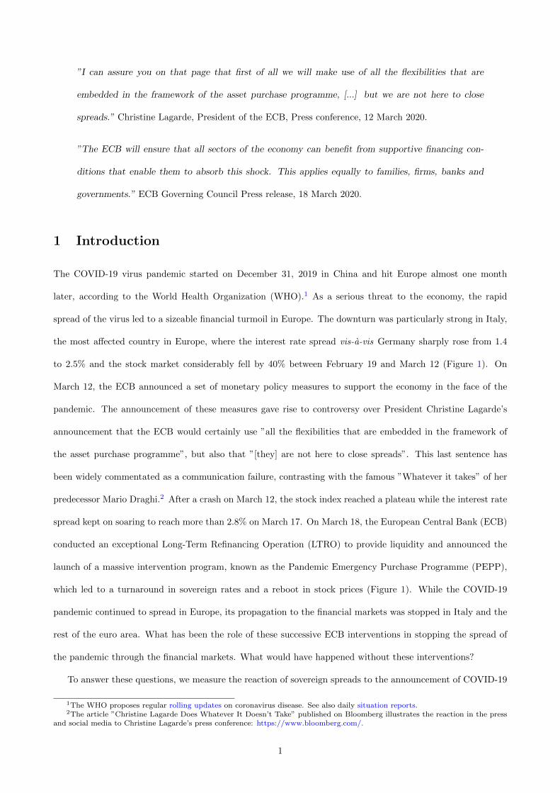
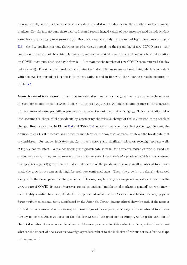
Figure 2 shows the growth rate of ECB total assets (in percentage, at a weekly frequency) and the respective

contribution of the two main open market operations: ”LTROs” and ”Securities held for monetary policy

purposes”. The category ”Others” gathers all other assets of the ECB balance sheet. Unfortunately, these

series are not available on a daily basis and cannot be decomposed into national shares.15 However, they

provide several helpful insights for interpreting our results.

ECB interventions can be classified as communication only on March 12 and as a mix of communication and

market operations on March 18. Indeed, the ECB balance sheet expansion starts the week that ends on March

20 and not on March 13. Then, the ECB intervention on March 12 can be considered as a communication

policy only, without significant market operations. This is not the case for the ECB press conference on March

18. At this date, the ECB provides exceptional LTROs of AC109.1305 bn for 98 days16 which implies a huge

increase of 17.73% for LTROs when compared with the previous week. Considering the full balance sheet, this

explains half of the 4.74% increase in total assets on March 20–which is composed from 2.31% from LTROs,

13https://www.ecb.europa.eu/press/pr/html/index.en.html14Simultaneously, the ECB states on March 18: “ The Governing Council was unanimous in its analysis that in addition to the

measures it decided on 12 March 2020, the ECB will continue to monitor closely the consequences for the economy of the spreadingcoronavirus and that the ECB stands ready to adjust all of its measures, as appropriate, should this be needed to safeguard liquidityconditions in the banking system and to ensure the smooth transmission of its monetary policy in all jurisdictions.”

15The ECB publishes a bimonthly breakdown of public sector securities under the PEPPhttps://www.ecb.europa.eu/mopo/implement/pepp/html/index.en.html

16There is also a MRO of AC1.4699 bn for 7 days this day, see the calendar of open market operations:https://www.ecb.europa.eu/mopo/implement/omo/html/top history.fr.html

8

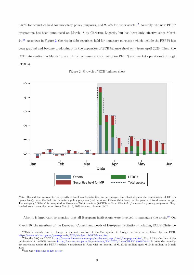
0.36% for securities held for monetary policy purposes, and 2.05% for other assets.17 Actually, the new PEPP

programme has been announced on March 18 by Christine Lagarde, but has been only effective since March

24.18 As shown in Figure 2, the rise in debt securities held for monetary purposes (which include the PEPP) has

been gradual and become predominant in the expansion of ECB balance sheet only from April 2020. Then, the

ECB intervention on March 18 is a mix of communication (mainly on PEPP) and market operations (through

LTROs).

Figure 2: Growth of ECB balance sheet

01

23

45

Jan Feb Mar Apr May JunDate

Others LTROs

Securities held for MP Total assets

Note: Dashed line represents the growth of total assets/liabilities, in percentage. Bar chart depicts the contribution of LTROs(green bars), Securities held for monetary policy purposes (red bars) and Others (blue bars) to the growth of total assets, in ppt.The category ”Others” is computed as Others = Total assets− (LTROs+ Securities held for monetary policy purposes). Greyshaded area covers the period from March 16, 2020 forward. Source: ECB.

Also, it is important to mention that all European institutions were involved in managing the crisis.19 On

March 10, the members of the European Council and heads of European institutions including ECB’s Christine

17This is mainly due to change in the net position of the Eurosystem in foreign currency as explained by the ECB:https://www.ecb.europa.eu/press/pr/wfs/2020/html/ecb.fs200324.en.html

18See the FAQ on PEPP https://www.ecb.europa.eu/mopo/implement/pepp/html/pepp-qa.en.html, March 24 is the date of thepublication of the ECB decision https://eur-lex.europa.eu/legal-content/EN/TXT/?uri=CELEX:32020D0440 In 2020, the monthlynet purchases under the PEPP reached a maximum in June with an amount of AC120321 million again AC15444 million in March2020

19See the “Timeline of EU action”.

9

Lagarde held a video conference on COVID-19. They discussed how to coordinate European Union efforts

to respond to the pandemic outbreak.20 We focus on ECB’s interventions, which came earlier and were more

commented on in terms of their effects on the sovereign debt markets. For example, the activation of the general

escape clause of the Stability and Growth Pact has been proposed by the European Commission on March 20,

and agreed by the Ministers of Finance of the Member States of the EU on March 23, that is after the main

ECB’s interventions.

The 5-25 March window. Based on the data and on the above-mentioned events, we focus on the 5-25

March period to identify when and how the sovereign interest rate response to the spread of the COVID-19

pandemic has changed. This choice is motivated by two reasons. First, March 5 occurred one business week

before the first ECB’s intervention (March 12), and March 25 occurred one week after the ECB’s decision of

March 18. Thus, the window is large enough such that we make sure that we do not miss any monetary policy

effect in our analysis. Second, on March 5, only a few countries reported deaths (France, Italy, Spain) while on

March 25, only Latvia, Malta and Slovakia did not report deaths for COVID-19. Thus, the window corresponds

to the period of the generalization of the pandemic in Europe. Lastly, in the remainder we take the series of

COVID-19 cases as a benchmark and not that of deaths. Since the number of confirmed cases precedes the

number of reported deaths, the series of COVID-19 cases provides more data for the estimation at the beginning

of the sample (on March 5, only six countries did not report cases, against fourteen for the series of deaths).

3 Methodology

Our primary interest is in the dynamic response of government spreads to the outbreak of the COVID-19

pandemic. To get an estimate of the response, we rely on the local projection method following Jorda (2005).

Considering the whole sample period, we estimate:

∆si,t+h = αi,h + ηt,h + βh∆xi,t + Γh(L)si,t−1 + Θh(L)zi,t + εi,t+h (1)

for country i and horizon h = 0, 1, . . . ,H, as of time t, where εi,t+h is the error term. ∆si,t+h ≡ si,t+h − si,t−1

is the variation of the 10-year government bond spread at horizon h. ∆xi,t ≡ xi,t− xi,t−1 is the daily change in

20Four priorities were identified at the end of the meeting: limiting the spread of the virus, the provision of medical equipment,promoting research (including research into a vaccine), and tackling socio-economic consequences. More details on the dedicatedmeeting webpage.

10

the number of total COVID-19 cases in country i as of time t. We consider the change in the number of cases

per 100,000 people. The main motivation for this choice is that the attention of observers has been focused

on the number of daily new cases per population since the beginning of the pandemic, sometimes in absolute

terms but never as a percentage of the number of total cases already reported, as illustrated by the very popular

figures published and massively distributed by the Financial Times. However, the robustness of our results are

checked when considering the daily change in the number of deaths per million people due to COVID-19, the

3-day rolling average of new cases, new cases in absolute terms, the lagged values of new cases, or the growth

rate of total cases as the independent variable ∆xi,t. Also, other robustness checks involve adding separately

the growth rate of total cases, the logarithm of the total number of cases, the first-difference of new cases, or

the lagged values of new cases as control variables in the baseline specification. Tables and figures containing

the results are given in Appendix. The coefficient of interest βh measures the variation of government spreads

h days after the release of data on new COVID-19 cases. A series of regression are estimated for each horizon

h. Since the model is estimated on a business daily basis, we assume that a one-week horizon is sufficiently long

to capture the path of the response coefficients βh. Then, we set H = 5.

To get an accurate estimate of these coefficients, we use a two-way fixed effects framework and add a set of

control variables as recommended by Herbst and Johannsen (2020).21 First, country-fixed effects αi,h take into

account the structural differences between countries. Second, time-fixed effects ηt,h absorb common features

across all countries but that change overtime, including the global evolution of the COVID-19 pandemic. Third,

the current value and the first four lags of the log of the stock index zi,t control for the state of the country-

economy and the effects of other news which could potentially have an impact on government spreads. Θh(L) is

a polynomial in the lag operator associated to the domestic stock markets, where Θh(L) =N−1∑n=0

θh,n+1Ln where

N stands for the number of lags. Finally, it also includes the first four lags of the dependent variable to control

for any serial correlation in the error term through the polynomial in the lag operator Γh(L) also defined by

Γh(L) =N−1∑n=0

γh,n+1Ln. We set N = 4 as the number of lags.

The linear local projection method described above can be transformed into a state-dependent model.

State-dependent local projection methods have been mainly applied to fiscal policy issues by Auerbach and

Gorodnichenko (2013) and Ramey and Zubairy (2018). As for the linear model, we estimate a series of regression

21Moreover, Herbst and Johannsen (2020) also suggest using large sample sizes to avoid bias in impulse responses estimated bylocal projections. We are in line with this recommendation since the size of our subsample exceeds 500 observations.

11

at each horizon h:

∆si,t+h = αi,h + ηt,h +Dt,t

[βa,h∆xi,t + Γa,h(L)si,t−1 + Θa,h(L)zi,t

](2)

+(1−Dt,t)[βb,h∆xi,t + Γb,h(L)si,t−1 + Θb,h(L)zi,t

]+ εi,t+h

where Dt,t is dummy variable that takes on 0 before a given date t, that is when t < t, and 1 thereafter, when

t ≥ t. The model is specified such that all the coefficients are state-dependent to account for the fact that

policy interventions had also an impact on country and time-fixed effects, and the link between sovereign bond

spreads and stock markets.

Equation (2) captures the dynamic response of government bond spreads to new COVID-19 cases conditional

on ECB’s intervention through the coefficients βa,h and βb,h. It is worth emphasizing that this is different from

the direct effect of a policy intervention on sovereign rates, which is gauged by the temporal fixed effect, ηt,h.

Since we are mostly interested in βa,h and βb,h coefficients, responses in period t+ h to new information on the

COVID-19 severity at time t, conditional on the state of the economy, are computed as in Born et al. (2019),

by the following expression:

∂∆si,t+h

∂∆xi,t

∣∣∣Dt,t

= Dt,t × βa,h + (1−Dt,t)× βb,h (3)

that is a linear combination of impulse response coefficients. As our aim is to investigate possible nonlinearities

in the response coefficient βh according to the state of the economy during the 5-25 March period window (see

Section 2), event-dummies are constructed according for t ∈ {3/5, ..., 3/25}.

4 Results

This section presents our main results to identify when the rise of COVID-induced sovereign bond spreads has

been severed.

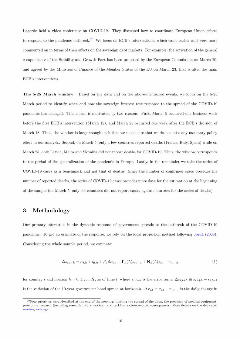
Results for the full sample. Let us start with the equation (1) for the full sample of observations. Figure 3

shows the path of the estimated coefficient βh and the 95% confidence interval and Table C.1 contains estimation

results. The response coefficient is slightly negative at all horizons. However, the magnitude of the effect is very

tiny: the change in interest rate spread is very close to zero at all horizons, and reaches −0.002 ppt at horizon

12

h = 3 for 10 new cases per million people. As shown by the confidence interval, the impact of new cases is

not significantly different from zero when we consider the full sample. As explained above, it does not mean

that policy interventions have no direct effects on sovereign interest rates22, but that these rates do not react

significantly to the occurrence of new COVID-19 cases. But what happens when the sample is split? Especially,

we draw attention to the period before ECB interventions.

Figure 3: Impulse responses of 10-year government bond spreads to new COVID-19 cases in the euro area-.0

04-.0

020

.002

0 1 2 3 4 5Days

Full sample

Note: Impulse responses represent βh coefficient from equation (1) and the grey shaded area represents the 95% confidence interval.

Figure 4: Impulse responses of 10-year government bond spreads to new COVID-19 cases in the euro area

-.10

.1.2

.3

0 1 2 3 4 5Horizon h

Before March 5

-.004

-.002

0.0

02.0

04

0 1 2 3 4 5Horizon h

After March 5

Note: Impulse responses are computed following equation (3). Left panel shows coefficient βb,h (before the splitting date), whereasright panel shows coefficient βa,h (after the splitting date). Grey shaded area represents the 95% confidence interval.

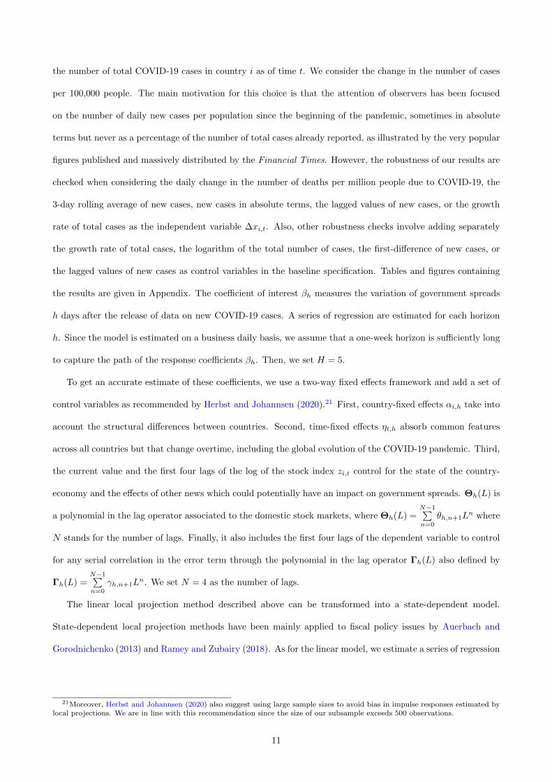
The difference between the beginning and the end of the 5-25 March window. Figure 4 compares

the response coefficients βb,h and βa,h of 10-year government spreads to new COVID-19 cases before and after

March 5 (t = 3/5, the first date of our window period). Before March 5, without any ECB’s intervention, the

22Indeed, as indicated in Figure C.1, time-fixed effects ηt,h are significantly negative around key ECB’s intervention dates,namely on March 12 and March 18.

13

response coefficient βb,h follows an explosive path. 10-year government bond spreads increase by more than

0.021 ppt for 10 new cases per million people on impact. This rise significantly accelerates to reach 0.240 ppt up

to 5 business days. This explosive path has severely threatened debt sustainability in the euro area as long as

the pandemic was spreading. On March 12, Italy reported 38.256 new cases per million residents, Spain 24.66

and France 7.614. Given this βb,5 estimate, considering only this single date would have led to a cumulative

increase in the spread over 5 days of 0.92 ppt in Italy, 0.59 ppt in Spain and 0.18 ppt in France for 10 new

cases per million people. After March 5, estimates on sample including ECB’s interventions show a response

coefficient βa,h very close to zero and not significant.

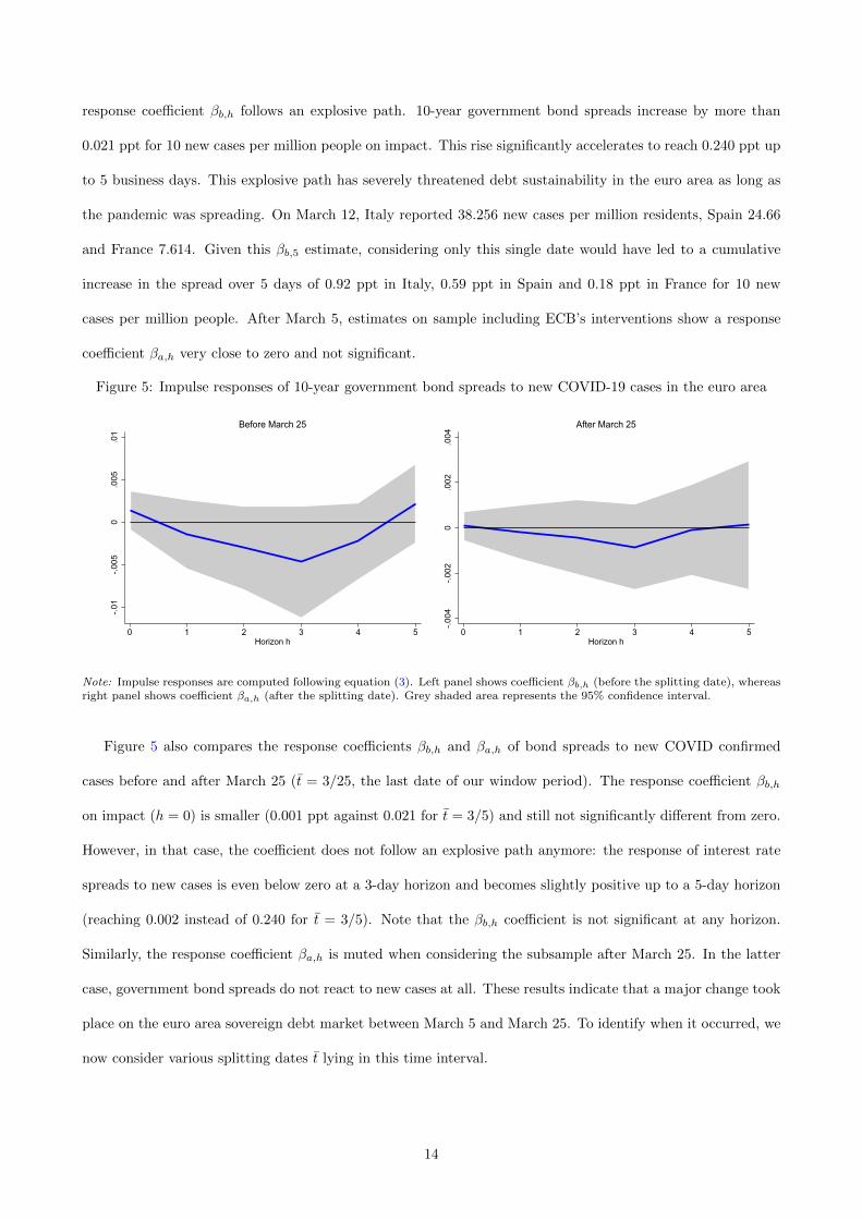
Figure 5: Impulse responses of 10-year government bond spreads to new COVID-19 cases in the euro area

-.01

-.005

0.0

05.0

1

0 1 2 3 4 5Horizon h

Before March 25

-.004

-.002

0.0

02.0

04

0 1 2 3 4 5Horizon h

After March 25

Note: Impulse responses are computed following equation (3). Left panel shows coefficient βb,h (before the splitting date), whereasright panel shows coefficient βa,h (after the splitting date). Grey shaded area represents the 95% confidence interval.

Figure 5 also compares the response coefficients βb,h and βa,h of bond spreads to new COVID confirmed

cases before and after March 25 (t = 3/25, the last date of our window period). The response coefficient βb,h

on impact (h = 0) is smaller (0.001 ppt against 0.021 for t = 3/5) and still not significantly different from zero.

However, in that case, the coefficient does not follow an explosive path anymore: the response of interest rate

spreads to new cases is even below zero at a 3-day horizon and becomes slightly positive up to a 5-day horizon

(reaching 0.002 instead of 0.240 for t = 3/5). Note that the βb,h coefficient is not significant at any horizon.

Similarly, the response coefficient βa,h is muted when considering the subsample after March 25. In the latter

case, government bond spreads do not react to new cases at all. These results indicate that a major change took

place on the euro area sovereign debt market between March 5 and March 25. To identify when it occurred, we

now consider various splitting dates t lying in this time interval.

14

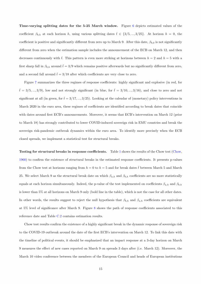
Time-varying splitting dates for the 5-25 March window. Figure 6 depicts estimated values of the

coefficient βb,h at each horizon h, using various splitting dates t ∈ {3/5, ..., 3/25}. At horizon h = 0, the

coefficient is positive and significantly different from zero up to March 9. After this date, βb,0 is not significantly

different from zero when the estimation sample includes the announcement of the ECB on March 12, and then

decreases continuously with t. This pattern is even more striking at horizons between h = 2 and h = 5 with a

first sharp fall in βb,h around t = 3/9 which remains positive afterwards but no significantly different from zero,

and a second fall around t = 3/18 after which coefficients are very close to zero.

Figure 7 summarizes the three regimes of response coefficients: highly significant and explosive (in red, for

t = 3/5, ..., 3/9), low and not strongly significant (in blue, for t = 3/10, ..., 3/16), and close to zero and not

significant at all (in green, for t = 3/17, ..., 3/25). Looking at the calendar of (monetary) policy interventions in

March 2020 in the euro area, these regimes of coefficients are identified according to break dates that coincide

with dates around first ECB’s announcements. Moreover, it seems that ECB’s intervention on March 12 (prior

to March 18) has strongly contributed to lower COVID-induced sovereign risk in EMU countries and break the

sovereign risk-pandemic outbreak dynamics within the euro area. To identify more precisely when the ECB

closed spreads, we implement a statistical test for structural breaks.

Testing for structural breaks in response coefficients. Table 1 shows the results of the Chow test (Chow,

1960) to confirm the existence of structural breaks in the estimated response coefficients. It presents p-values

from the Chow test at horizons ranging from h = 0 to h = 5 and for break dates t between March 5 and March

25. We select March 9 as the structural break date on which βa,h and βb,h coefficients are no more statistically

equals at each horizon simultaneously. Indeed, the p-value of the test implemented on coefficients βa,h and βb,h

is lower than 5% at all horizons on March 9 only (bold line in the table), which is not the case for all other dates.

In other words, the results suggest to reject the null hypothesis that βb,h and βa,h coefficients are equivalent

at 5% level of significance after March 9. Figure 8 shows the path of response coefficients associated to this

reference date and Table C.2 contains estimation results.

Chow test results confirm the existence of a highly significant break in the dynamic response of sovereign risk

to the COVID-19 outbreak around the date of the first ECB’s intervention on March 12. To link this date with

the timeline of political events, it should be emphasized that an impact response at a 3-day horizon on March

9 measures the effect of new cases reported on March 9 on spreads 3 days after (i.e. March 12). Moreover, the

March 10 video conference between the members of the European Council and heads of European institutions

15

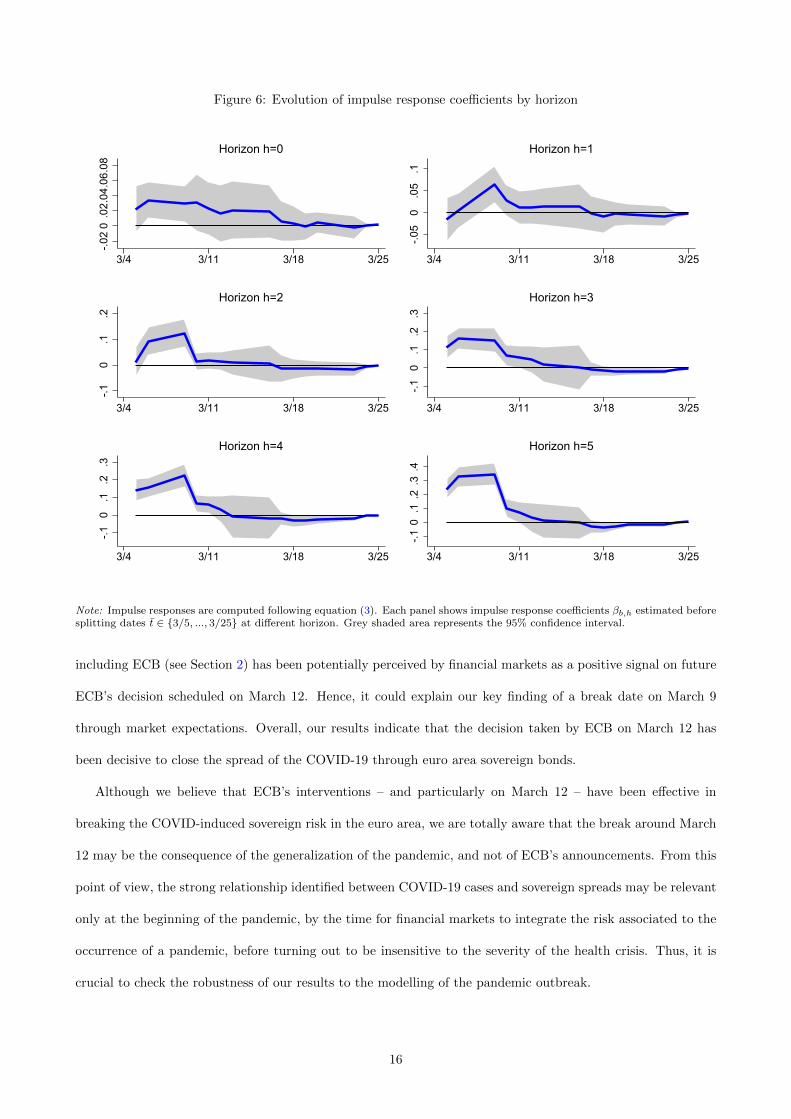
Figure 6: Evolution of impulse response coefficients by horizon-.0

20

.02.

04.0

6.08

3/4 3/11 3/18 3/25

Horizon h=0

-.05

0.0

5.1

3/4 3/11 3/18 3/25

Horizon h=1

-.10

.1.2

3/4 3/11 3/18 3/25

Horizon h=2

-.10

.1.2

.33/4 3/11 3/18 3/25

Horizon h=3

-.10

.1.2

.3

3/4 3/11 3/18 3/25

Horizon h=4

-.10

.1.2

.3.4

3/4 3/11 3/18 3/25

Horizon h=5

Note: Impulse responses are computed following equation (3). Each panel shows impulse response coefficients βb,h estimated beforesplitting dates t ∈ {3/5, ..., 3/25} at different horizon. Grey shaded area represents the 95% confidence interval.

including ECB (see Section 2) has been potentially perceived by financial markets as a positive signal on future

ECB’s decision scheduled on March 12. Hence, it could explain our key finding of a break date on March 9

through market expectations. Overall, our results indicate that the decision taken by ECB on March 12 has

been decisive to close the spread of the COVID-19 through euro area sovereign bonds.

Although we believe that ECB’s interventions – and particularly on March 12 – have been effective in

breaking the COVID-induced sovereign risk in the euro area, we are totally aware that the break around March

12 may be the consequence of the generalization of the pandemic, and not of ECB’s announcements. From this

point of view, the strong relationship identified between COVID-19 cases and sovereign spreads may be relevant

only at the beginning of the pandemic, by the time for financial markets to integrate the risk associated to the

occurrence of a pandemic, before turning out to be insensitive to the severity of the health crisis. Thus, it is

crucial to check the robustness of our results to the modelling of the pandemic outbreak.

16

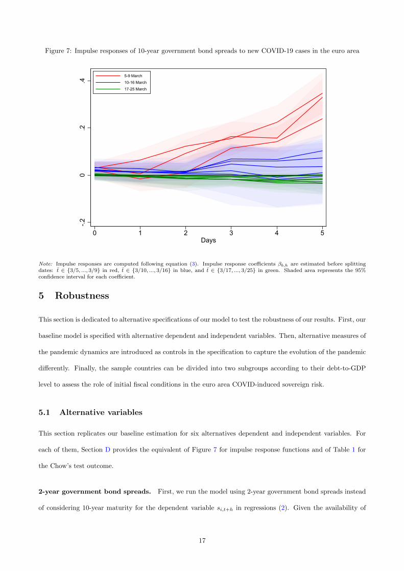
Figure 7: Impulse responses of 10-year government bond spreads to new COVID-19 cases in the euro area

-.20

.2.4

0 1 2 3 4 5Days

5-9 March10-16 March17-25 March

Note: Impulse responses are computed following equation (3). Impulse response coefficients βb,h are estimated before splittingdates: t ∈ {3/5, ..., 3/9} in red, t ∈ {3/10, ..., 3/16} in blue, and t ∈ {3/17, ..., 3/25} in green. Shaded area represents the 95%confidence interval for each coefficient.

5 Robustness

This section is dedicated to alternative specifications of our model to test the robustness of our results. First, our

baseline model is specified with alternative dependent and independent variables. Then, alternative measures of

the pandemic dynamics are introduced as controls in the specification to capture the evolution of the pandemic

differently. Finally, the sample countries can be divided into two subgroups according to their debt-to-GDP

level to assess the role of initial fiscal conditions in the euro area COVID-induced sovereign risk.

5.1 Alternative variables

This section replicates our baseline estimation for six alternatives dependent and independent variables. For

each of them, Section D provides the equivalent of Figure 7 for impulse response functions and of Table 1 for

the Chow’s test outcome.

2-year government bond spreads. First, we run the model using 2-year government bond spreads instead

of considering 10-year maturity for the dependent variable si,t+h in regressions (2). Given the availability of

17

Figure 8: Impulse responses of 10-year government bond spreads to new COVID-19 cases in the euro area0

.1.2

.3.4

0 1 2 3 4 5Horizon h

Before March 9

-.004

-.002

0.0

02.0

04

0 1 2 3 4 5Horizon h

After March 9

Note: Impulse responses are computed following equation (3). Left panel shows coefficient βb,h (before the splitting date), whereasright panel shows coefficient βa,h (after the splitting date). Grey shaded area represents the 95% confidence interval.

the data presented in Appendix A and Appendix B, the list of euro area countries in our sample is restricted to

Austria, Belgium, Finland, France, Ireland, Italy, Latvia, Netherlands, Portugal, Slovakia, Slovenia, and Spain.

Moreover, some 2-year government bond yields data are missing for Ireland and Slovakia at the beginning of

the sample period. However, those changes in the composition of our sample do not contradict our results: the

response coefficient of sovereign spreads to the pandemic outbreak has been explosive before March 9, small

between March 10 and March 16, and almost muted thereafter, as shown in Figure D.1. According to the Chow

test results in Table D.1, the regime switches one day later (on March 10) than in our benchmark results.

New deaths. Then, we replace the number of new confirmed cases by the number of new deaths due to

COVID-19 as a relevant measure of the pandemic severity to be in line with Eichenbaum et al. (2020) for the

independent variable xi,t in regressions (2). The variable is now constructed as the total number of new deaths

per million inhabitants. Figure D.2 shows that before March 9, the response coefficient of sovereign spreads

to new deaths due to COVID-19 has been steeper comparing to that considering new cases in the baseline

regression. The value of βb,h with new deaths up to a 5-day horizon reaches 0.916. It is almost thrice the value

of the response coefficient to new cases shown previously. After March 9, the βa,h response coefficient is quite

similar to that estimated in the baseline specification. However, it is significantly different from zero at horizon

3 in the case where we consider new deaths instead of new cases in the estimates. The results of the Chow test

in Table D.2 suggest significant differences in the response coefficients up to March 11.

18

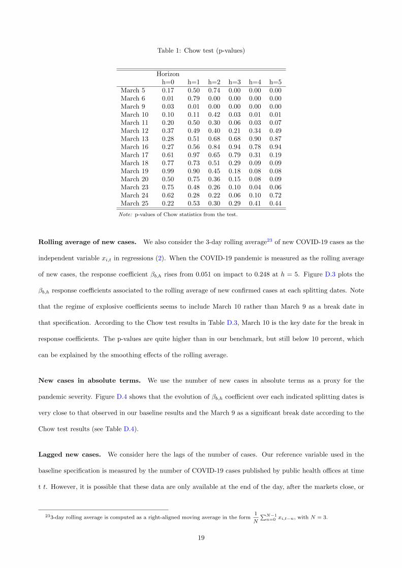
Table 1: Chow test (p-values)

Horizonh=0 h=1 h=2 h=3 h=4 h=5

March 5 0.17 0.50 0.74 0.00 0.00 0.00March 6 0.01 0.79 0.00 0.00 0.00 0.00March 9 0.03 0.01 0.00 0.00 0.00 0.00March 10 0.10 0.11 0.42 0.03 0.01 0.01March 11 0.20 0.50 0.30 0.06 0.03 0.07March 12 0.37 0.49 0.40 0.21 0.34 0.49March 13 0.28 0.51 0.68 0.68 0.90 0.87March 16 0.27 0.56 0.84 0.94 0.78 0.94March 17 0.61 0.97 0.65 0.79 0.31 0.19March 18 0.77 0.73 0.51 0.29 0.09 0.09March 19 0.99 0.90 0.45 0.18 0.08 0.08March 20 0.50 0.75 0.36 0.15 0.08 0.09March 23 0.75 0.48 0.26 0.10 0.04 0.06March 24 0.62 0.28 0.22 0.06 0.10 0.72March 25 0.22 0.53 0.30 0.29 0.41 0.44

Note: p-values of Chow statistics from the test.

Rolling average of new cases. We also consider the 3-day rolling average23 of new COVID-19 cases as the

independent variable xi,t in regressions (2). When the COVID-19 pandemic is measured as the rolling average

of new cases, the response coefficient βb,h rises from 0.051 on impact to 0.248 at h = 5. Figure D.3 plots the

βb,h response coefficients associated to the rolling average of new confirmed cases at each splitting dates. Note

that the regime of explosive coefficients seems to include March 10 rather than March 9 as a break date in

that specification. According to the Chow test results in Table D.3, March 10 is the key date for the break in

response coefficients. The p-values are quite higher than in our benchmark, but still below 10 percent, which

can be explained by the smoothing effects of the rolling average.

New cases in absolute terms. We use the number of new cases in absolute terms as a proxy for the

pandemic severity. Figure D.4 shows that the evolution of βb,h coefficient over each indicated splitting dates is

very close to that observed in our baseline results and the March 9 as a significant break date according to the

Chow test results (see Table D.4).

Lagged new cases. We consider here the lags of the number of cases. Our reference variable used in the

baseline specification is measured by the number of COVID-19 cases published by public health offices at time

t t. However, it is possible that these data are only available at the end of the day, after the markets close, or

233-day rolling average is computed as a right-aligned moving average in the form1

N

∑N−1n=0 xi,t−n, with N = 3.

19

even on the day after. In that case, it is the values recorded on the day before that matters for the financial

markets. To take into account these delays, first and second lagged values of new cases are used as independent

variables xi,t−1 or xi,t−2 in regressions (2). Results are reported only for the second lag of new cases in Figure

D.5 – the βb,h coefficient is now the response of sovereign spreads to the second lag of new COVID cases – and

confirm our narrative of the crisis. By doing so, we assume that at time t, financial markets have information

on COVID cases published the day before (t− 1) containing the number of new COVID cases reported the day

before (t− 2). The structural break occurred later than March 9, our reference break date, which is consistent

with the two lags introduced in the independent variable and in line with the Chow test results reported in

Table D.5.

Growth rate of total cases. In our baseline estimation, we consider ∆xi,t as the daily change in the number

of cases per million people between t and t − 1, denoted xi,t. Here, we take the daily change in the logarithm

of the number of cases per million people as an alternative variable, that is ∆ log xi,t. This specification takes

into account the shape of the pandemic by considering the relative change of the xi,t instead of its absolute

change. Results reported in Figure D.6 and Table D.6 indicate that when considering the log-difference, the

occurrence of COVID-19 cases has no significant effects on the sovereign spreads, whatever the break date that

is considered. Our model indicates that ∆xi,t has a strong and significant effect on sovereign spreads while

∆ log xi,t has no effect. While considering the growth rate is usual for economic variables with a trend (as

output or prices), it may not be relevant to use it to measure the outbreak of a pandemic which has a stretched

S-shaped (or sigmoid) growth curve. Indeed, at the eve of the pandemic, the very small number of total cases

made the growth rate extremely high for each new confirmed cases. Then, the growth rate sharply decreased

along with the development of the pandemic. This may explain why sovereign markets do not react to the

growth rate of COVID-19 cases. Moreover, sovereign markets (and financial markets in general) are well-known

to be highly sensitive to news published in the press and social media. As mentioned before, the very popular

figures published and massively distributed by the Financial Times (among others) show the path of the number

of total or new cases in absolute terms, but never in growth rate (as a percentage of the number of total cases

already reported). Since we focus on the first few weeks of the pandemic in Europe, we keep the variation of

the total number of cases as our benchmark. Moreover, we consider this series in extra specifications to test

whether the impact of new cases on sovereign spreads is robust to the inclusion of various controls for the shape

of the pandemic.

20

5.2 Controlling for the shape of the pandemic

Our baseline regression (2) is extended to include additional controls. Using the reference date, we investigate

whether these controls may alter our estimate of βa,h and βb,h for the reference date t. The specification now

takes the following form:

∆si,t+h = αi,h + ηt,h +Dt,t

[βa,h∆xi,t + Ψa,h(L)Xi,t + Γa,h(L)si,t−1 + Θa,h(L)zi,t

](4)

+(1−Dt,t)[βb,h∆xi,t + Ψb,h(L)Xi,t + Γb,h(L)si,t−1 + Θb,h(L)zi,t

]+ εi,t+h

where Ψ•,h(L) is a polynomial in the lag operator associated to the control variable Xi,t defined hereafter.

Results are reported in regression tables in Appendix F.24 The symbol • accounts for both after a and before b

estimated coefficients.

Growth rate of total cases. First, we control for the growth rate of the number of total cases. The growth

rate of total cases is measured as the first-difference (daily change) of the logarithm of the number of total

cases. Hence, Xi,t = ∆ log xi,t. Moreover, since no lagged value of controls is included in the estimate, we set

Ψ•,h(L) =N∑

n=0ψ•,hL

n, with N = 0. Table E.1 shows that including the growth rate of the number of total

cases in the model does not alter our baseline results. The ψb,h coefficient is close to zero and not significant at

all over the horizon.

Logarithm of total cases. We also control for the logarithm of the number of total cases to take into account

the state of the ongoing pandemic in its effect on sovereign bond spreads. Hence, Xi,t = log xi,t. As in the

previous case, we set Ψ•,h(L) =N∑

n=0ψ•,hL

n, with N = 0. Table E.2 shows that including the log of total cases

per population in the model does not alter our baseline results, even if the ψb,h coefficient is significantly positive

up to horizon h = 4.

Lagged values of new cases. Then, we control for lagged values of new COVID cases, and we estimate

equation (4) setting Ψ•,h(L) =N−1∑n=0

ψ•,h,n+1Ln, with N = 2. The control variable is expressed as Xi,t = ∆xi,t−1,

where ∆xi,t−1 ≡ xi,t−1−xi,t−2. The lagged values of new cases are measured as the first and second lags of new

cases per 100,000 people. Table E.3 reports the results. The βb,h coefficient is not as strong and statistically

significant as in our baseline estimates. Note that both coefficients on first and second lagged values of new

24March 9 is chosen as the break date in all the regression tables to allow for comparison with our baseline results. Figuresdepicting impulse response functions and Chow test tables are available upon request.

21

cases, ψb,h,1 and ψb,h,2 respectively, are often significant over the horizon. This is especially true for the ψb,h,2

coefficient. By doing so, we capture the persistence of new COVID confirmed cases on government bond spreads.

First-difference of new cases. Finally, we use the ”variation of the variation” of new COVID-19 cases

to account for the stretched S-shaped dynamics of the pandemic. Then, Xi,t = ∆xi,t − ∆xi,t−1 which is

positive in the first phase of the pandemic outbreak and negative at the end. The new cases variable (in

first-difference) is now measured as the daily change in the number of new cases per 100,000 people. Also,

we set Ψ•,h(L) =N∑

n=0ψ•,hL

n, with N = 0. We then estimate equation (4). Results in Table E.4 show that

including the first-difference of new cases as a control variable does not change our baseline results that much.

Note however that the ψb,h coefficient is significantly positive on impact and turns out to be negative over the

horizon, but is constantly lower than the estimated βb,h.

5.3 Public debt-to-GDP

Delatte and Guillaume (2020) and Augustin et al. (2020) among others highlight the key role of initial fiscal

conditions in the sovereign debt markets reaction to the pandemic outbreak. To investigate the role of country

fiscal conditions, we run the regressions defined by equation (2) for two subsamples of countries. The first

subsample is referred to ’high debt/GDP’ and consists in countries for which the debt-to-GDP ratio is above

the median calculated for all the sample in the end of 2019: Belgium, Cyprus, Spain, France, Greece, Italy, and

Portugal. The second subsample is referred to ’low debt/GDP’, for countries with a ratio below the median:

Austria, Finland, Ireland, Lithuania, Malta, Netherlands, Slovenia, and Slovakia.

Figure F.1 reports the results for our benchmark splitting date, that is on March 9. As Delatte and Guillaume

(2020) and Augustin et al. (2020), we observe a substantial heterogeneity in the response of bond spreads to

new COVID-19 cases which are positive and significant in the high debt/GDP subsample, but not significantly

different from zero in the low debt/GDP subsample of countries. We then investigate whether this heterogeneity

alters our narrative of the crisis. To do so, we conduct a Chow test to identify structural breaks between the

coefficients βa,h and βb,h in high debt/GDP countries only. Results are reported in Table F.1. The test results

indicate that the null hypothesis is now rejected at the 10% level of significance after March 9. As for the full

sample, March 9 turns out to be the key reference date after which the sovereign debt markets no longer react

to the development of the pandemic.

22

6 Extensions

This section extends the analysis to four issues. First, we assess the distinctive roles of communication and

market operations channels in ECB’s interventions. Second, we question whether the ECB stopped the euro

area stock market crash. Third, we assess the existence of spillovers from the Italian pandemic outbreak to

the other European sovereign markets. Four, and lastly, we investigate what would have happened without the

structural break identified in the sovereign market reaction to the occurrence of new COVID cases.

6.1 What were the roles of communication and market operations channels in

ECB’s interventions?

We identify a structural change in the response of sovereign spreads to the COVID-19 pandemic outbreak on

March 9. Up to this date, COVID-19 new cases have a significant effect on sovereign spreads on the following

days. We consider the ECB announcements on March 12 as a credible explanation of this structural change.

In this section, we investigate the expansion of the ECB balance sheet to assess whether these announcements

had effects through a signaling channel.

Under the interpretation of ECB interventions’ narrative detailed in Section 2, our previous results support

the effectiveness of the communication channel associated to the March 12 press conference. In addition to our

results presented in Section 4, we also provide evidence based on the analysis of time-fixed effects. Figure C.1

depicts the time-fixed effects, using the outcome of the regression (1) for h = 0, which represents the common

trend in sovereign yields. It can be observed that the dates on which the spreads fall sharply coincide with

dates around ECB’s interventions on March 12 and March 18. As explained above, the March 12 fall can be

associated to a communication channel only, while the March 18 fall can be explained as the outcome of both

PEPP announcement and LTROs.

Then, we attempt to estimate the effects of ECB market operations on the sovereign yields responses to

the pandemic outbreak. This objective is challenging due to the lack of daily and national data on market

operations, especially through LTROs. Then, we simplify our empirical framework by considering only h = 0.

Indeed, using weekly data of ECB balance sheet, we avoid the risk of overlapping weeks with different monetary

policy stance by considering only the daily change in sovereign yields in response to COVID-19 new cases. We

23

then estimate

∆si,t = αi + ηt +Dt,t

[βa∆xi,t + µa∆xi,t × bt + Γa(L)si,t−1 + Θa(L)zi,t

](5)

+(1−Dt,t)[βb∆xi,t + µb∆xi,t × bt + Γb(L)si,t−1 + Θb(L)zi,t

]+ εi,t

with notation described in Section 3, and bt = 100×( bi,t−bi,t−5

bi,t−5

)denotes the weekly growth rate in percentage

of the b-category of ECB assets (namely LTROs, Securities, and Total). This growth rate is the same for all

business days of a week given the amount of assets published by the ECB for the Friday of this week. The

impact of COVID-19 new cases on sovereign spreads is now conditional on the break date and the stance of

monetary policy at this date

∂∆si,t∂∆xi,t

∣∣∣Dt,t

= Dt,t

[βa + µa × bt

]+ (1−Dt,t)

[βb,h + µb × bt

](6)

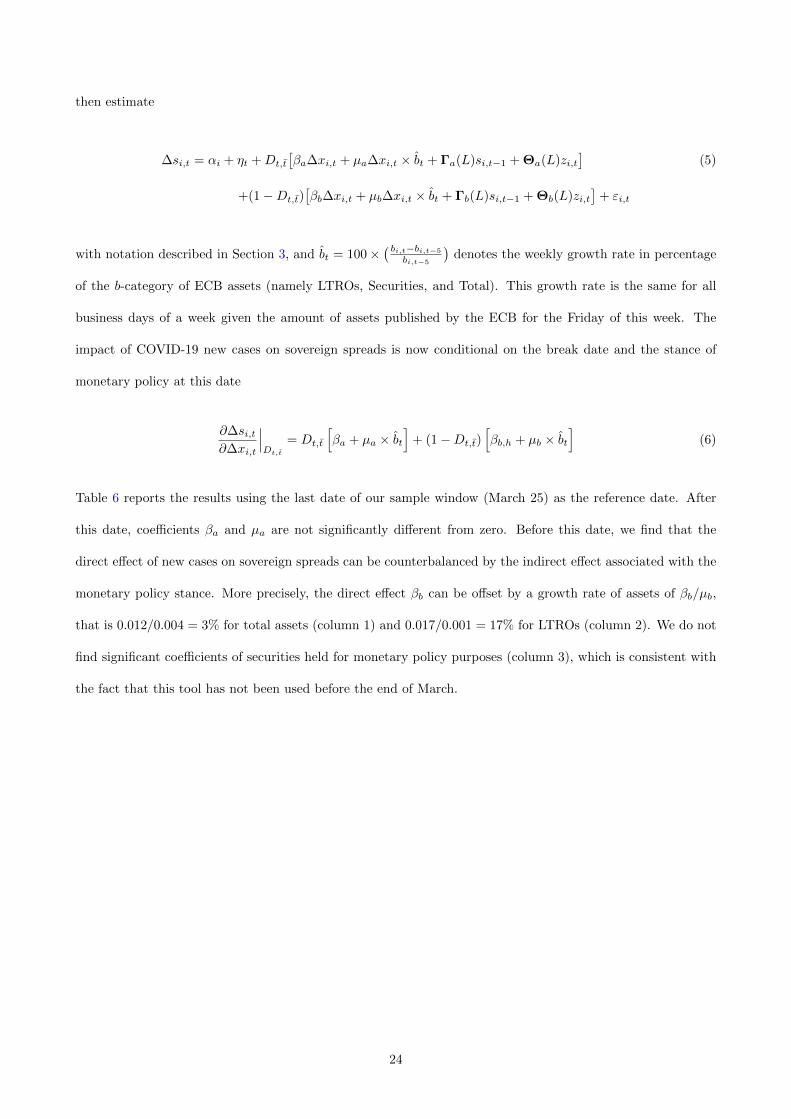
Table 6 reports the results using the last date of our sample window (March 25) as the reference date. After

this date, coefficients βa and µa are not significantly different from zero. Before this date, we find that the

direct effect of new cases on sovereign spreads can be counterbalanced by the indirect effect associated with the

monetary policy stance. More precisely, the direct effect βb can be offset by a growth rate of assets of βb/µb,

that is 0.012/0.004 = 3% for total assets (column 1) and 0.017/0.001 = 17% for LTROs (column 2). We do not

find significant coefficients of securities held for monetary policy purposes (column 3), which is consistent with

the fact that this tool has not been used before the end of March.

24

Table 2: Dependent variable 10-year spread (before and after March 25)

Day 0 Day 0 Day 0

new cases – before 0.012∗∗ 0.017∗∗ 0.004(0.00) (0.01) (0.03)

new cases – after -0.000 0.000 -0.001(0.00) (0.00) (0.00)

new cases x growth of total assets – before -0.004∗∗

(0.00)

new cases x growth of total assets – after 0.000(0.00)

new cases x growth of LTROs – before -0.001∗∗

(0.00)

new cases x growth of LTROs – after -0.000(0.00)

new cases x growth of securities held for MP – before -0.003(0.03)

new cases x growth of securities held for MP – after 0.001∗

(0.00)

R2 0.493 0.493 0.490Observations 1374 1374 1374

Note: ∗ p < 0.10, ∗∗ p < 0.05, ∗∗∗ p < 0.01. Clustered standard errors by country in parentheses. Thistable reports the βb, βa, µb, µa coefficients introduced in the regression equation (5) for t = {3/25}.The new cases variable is measured as the daily change in the number of total cases per 100,000 people.Total assets, LTROs, and Securities held for monetary policy purposes (MP) growth rates are computedat a business daily frequency and are given in percentage.

6.2 Did the ECB stop the euro area stock market crash?

In this section, we extend our empirical strategy to assess the dynamic effect of COVID-19 outbreak on the stock

markets in the euro area. So far we have included equity market data as a control variable in our regressions

for sovereign spreads in order to measure their reaction to announcements of new cases of COVID-19 given all

the information already anticipated by the markets.25 Cox et al. (2020) find evidence that Federal Reserve’s

announcements have been decisive in the reversal of the US equity markets in March and April after the market

crash of February. At that time, only a tiny fraction of the credit announced was distributed, leading the

authors to conclude that market movements have been the outcome of a shift in investors’ risk-aversion.

To investigate the response of the stock market to new cases in the euro area, the model defined by equation

(1) now takes the form:

∆zi,t+h = αi,h + ηt,h + βh∆xi,t + Γh(L)zi,t−1 + Θh(L)si,t + εi,t+h (7)

25Davis et al. (2021) shows that stock market foreshadows workplace mobility.

25

with notation described in Section 3. The dependent variable is written ∆zi,t+h ≡ zi,t+h − zi,t−1 and is the

variation of the log of the stock index (i.e. the cumulative logarithmic return) at horizon h. The coefficient of

interest βh is the response of the national stock index to the pandemic outbreak. The model is still specified

with country and time-fixed effects and a set of control variables including the first four lags of the dependent

variable and the current and four past values of 10-year sovereign bond spreads. The horizon remains for 5

days, H = 5.

Figure 9: Impulse responses of stock market indices (in log) to new COVID-19 cases in the euro area

-.2-.1

5-.1

-.05

0

0 1 2 3 4 5Days

5-9 March10-16 March17-25 March

Note: Impulse responses represent βb,h coefficient from equation (8). Impulse response coefficients βb,h are estimated beforesplitting dates: t ∈ {3/5, ..., 3/9} in red, t ∈ {3/10, ..., 3/16} in blue, and t ∈ {3/17, ..., 3/25} in green. Shaded area represents the95% confidence interval for each coefficient.

In the spirit of equation (2), the state-dependent local projections framework is now expressed as follows:

∆zi,t+h = αi,h + ηt,h +Dt,t

[βa,h∆xi,t + Γa,h(L)zi,t−1 + Θa,h(L)si,t

](8)

+(1−Dt,t)[βb,h∆xi,t + Γb,h(L)zi,t−1 + Θb,h(L)si,t

]+ εi,t+h

where Dt,t is dummy variable that takes on 0 before a given date t, that is when t < t, and 1 thereafter, when

t ≥ t. Here again, these event-dummies are constructed according for t ∈ {3/5, ..., 3/25}. We employ exactly

the same procedure than that developed in Section 4: comparing impulse response coefficients βa,h and βb,h

26

setting splitting dates on March 5 (t = 3/5) and March 25 (t = 3/25), focusing on the path of βb,h when the

model runs over various splitting dates t ∈ {3/5, ..., 3/25}, and testing for structural changes in the response

coefficients overtime.

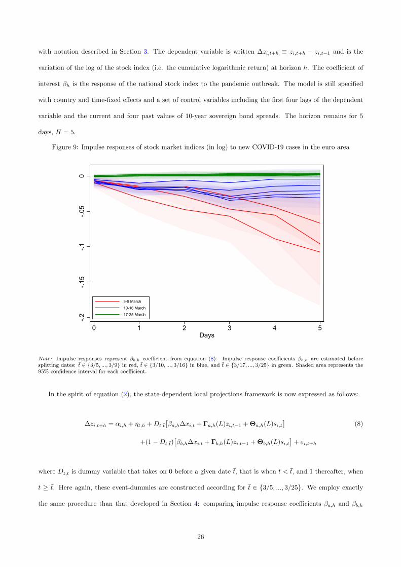
Results are presented in Appendix G and summarized in Figure 9 that replicates Figure 7 for the cumulated

stock market return instead of the sovereign spread. Up to March 9, the stock market response to new COVID-

19 cases is explosive with a cumulative fall of 11% in the stock market index 5 days after the occurrence of

new cases. The response is no longer explosive thereafter (blue lines), and finally completely muted when the

last dates of the period window are considered (green lines). Hence, ECB’s interventions have not only closed

spreads in the euro area, but also prevented an even more dramatic stock market crash. Given the timing of

balance sheet expansion explained in Section 6.1, these results also support the existence of the communication

channel of the ECB intervention on stock markets–as reported in Cox et al. (2020) for the US economy– since

there is no significant balance sheet expansion before March 18.

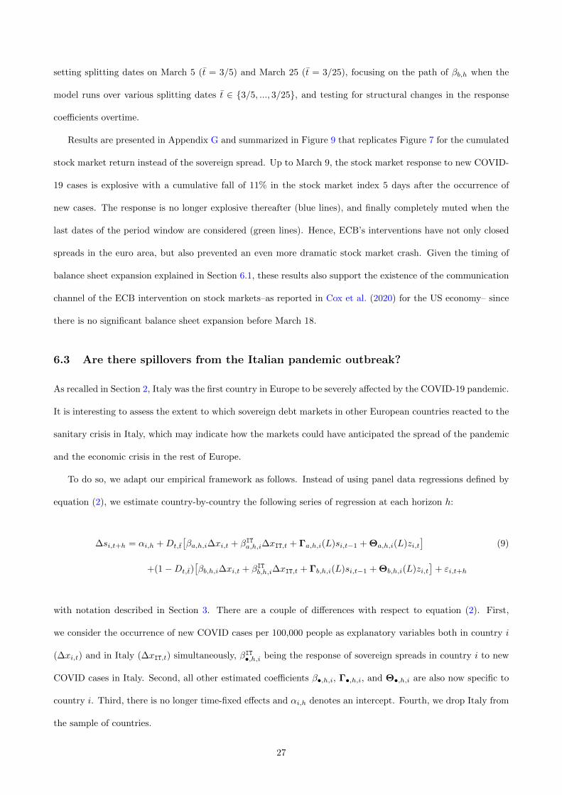
6.3 Are there spillovers from the Italian pandemic outbreak?

As recalled in Section 2, Italy was the first country in Europe to be severely affected by the COVID-19 pandemic.

It is interesting to assess the extent to which sovereign debt markets in other European countries reacted to the

sanitary crisis in Italy, which may indicate how the markets could have anticipated the spread of the pandemic

and the economic crisis in the rest of Europe.

To do so, we adapt our empirical framework as follows. Instead of using panel data regressions defined by

equation (2), we estimate country-by-country the following series of regression at each horizon h:

∆si,t+h = αi,h +Dt,t

[βa,h,i∆xi,t + βITa,h,i∆xIT,t + Γa,h,i(L)si,t−1 + Θa,h,i(L)zi,t

](9)

+(1−Dt,t)[βb,h,i∆xi,t + βITb,h,i∆xIT,t + Γb,h,i(L)si,t−1 + Θb,h,i(L)zi,t

]+ εi,t+h

with notation described in Section 3. There are a couple of differences with respect to equation (2). First,

we consider the occurrence of new COVID cases per 100,000 people as explanatory variables both in country i

(∆xi,t) and in Italy (∆xIT,t) simultaneously, βIT•,h,i being the response of sovereign spreads in country i to new

COVID cases in Italy. Second, all other estimated coefficients β•,h,i, Γ•,h,i, and Θ•,h,i are also now specific to

country i. Third, there is no longer time-fixed effects and αi,h denotes an intercept. Fourth, we drop Italy from

the sample of countries.

27

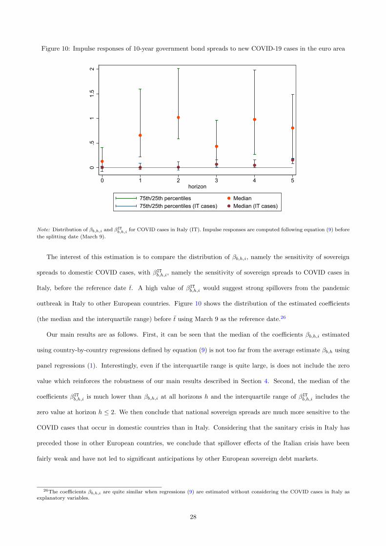
Figure 10: Impulse responses of 10-year government bond spreads to new COVID-19 cases in the euro area

0.5

11.

52

0 1 2 3 4 5horizon

75th/25th percentiles Median75th/25th percentiles (IT cases) Median (IT cases)

Note: Distribution of βb,h,i and βITb,h,i for COVID cases in Italy (IT). Impulse responses are computed following equation (9) before

the splitting date (March 9).

The interest of this estimation is to compare the distribution of βb,h,i, namely the sensitivity of sovereign

spreads to domestic COVID cases, with βITb,h,i, namely the sensitivity of sovereign spreads to COVID cases in

Italy, before the reference date t. A high value of βITb,h,i would suggest strong spillovers from the pandemic

outbreak in Italy to other European countries. Figure 10 shows the distribution of the estimated coefficients

(the median and the interquartile range) before t using March 9 as the reference date.26

Our main results are as follows. First, it can be seen that the median of the coefficients βb,h,i estimated

using country-by-country regressions defined by equation (9) is not too far from the average estimate βb,h using

panel regressions (1). Interestingly, even if the interquartile range is quite large, is does not include the zero

value which reinforces the robustness of our main results described in Section 4. Second, the median of the

coefficients βITb,h,i is much lower than βb,h,i at all horizons h and the interquartile range of βITb,h,i includes the

zero value at horizon h ≤ 2. We then conclude that national sovereign spreads are much more sensitive to the

COVID cases that occur in domestic countries than in Italy. Considering that the sanitary crisis in Italy has

preceded those in other European countries, we conclude that spillover effects of the Italian crisis have been

fairly weak and have not led to significant anticipations by other European sovereign debt markets.

26The coefficients βb,h,i are quite similar when regressions (9) are estimated without considering the COVID cases in Italy asexplanatory variables.

28

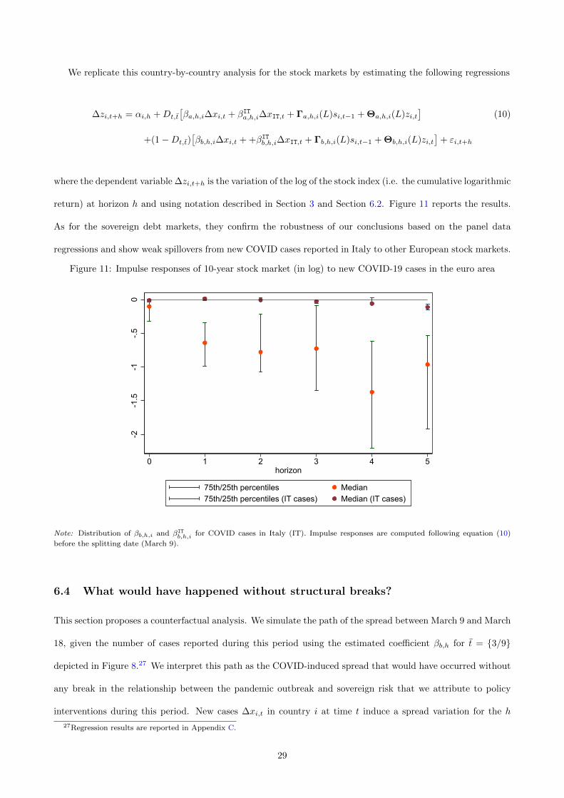
We replicate this country-by-country analysis for the stock markets by estimating the following regressions

∆zi,t+h = αi,h +Dt,t

[βa,h,i∆xi,t + βITa,h,i∆xIT,t + Γa,h,i(L)si,t−1 + Θa,h,i(L)zi,t

](10)

+(1−Dt,t)[βb,h,i∆xi,t + +βITb,h,i∆xIT,t + Γb,h,i(L)si,t−1 + Θb,h,i(L)zi,t

]+ εi,t+h

where the dependent variable ∆zi,t+h is the variation of the log of the stock index (i.e. the cumulative logarithmic

return) at horizon h and using notation described in Section 3 and Section 6.2. Figure 11 reports the results.

As for the sovereign debt markets, they confirm the robustness of our conclusions based on the panel data

regressions and show weak spillovers from new COVID cases reported in Italy to other European stock markets.

Figure 11: Impulse responses of 10-year stock market (in log) to new COVID-19 cases in the euro area

-2-1

.5-1

-.50

0 1 2 3 4 5horizon

75th/25th percentiles Median75th/25th percentiles (IT cases) Median (IT cases)

Note: Distribution of βb,h,i and βITb,h,i for COVID cases in Italy (IT). Impulse responses are computed following equation (10)

before the splitting date (March 9).

6.4 What would have happened without structural breaks?

This section proposes a counterfactual analysis. We simulate the path of the spread between March 9 and March

18, given the number of cases reported during this period using the estimated coefficient βb,h for t = {3/9}

depicted in Figure 8.27 We interpret this path as the COVID-induced spread that would have occurred without

any break in the relationship between the pandemic outbreak and sovereign risk that we attribute to policy

interventions during this period. New cases ∆xi,t in country i at time t induce a spread variation for the h

27Regression results are reported in Appendix C.

29

period ahead denoted ∆sxi,t+h that is defined as follows

∆sxi,t+h ≡ βb,h∆xi,t (11)

for h = 0, 1, .,H. The COVID-induced spread deviation as of time t is then the sum of the values of new cases

reported H periods before weighted by the coefficient βb,h:

∆sxi,t =

H∑h=0

βb,h∆xi,t−h (12)

By definition, the spread at K periods ahead is equal to the initial value of the spread plus the cumulative sum

of spread variations. Then, the COVID-induced spread is given by:

sxi,t+K = si,t +

K∑k=0

H∑h=0

βb,h∆xi,t+k−h (13)

Figure 12 shows the evolution of sxi,t+K between March 9 and March 18 for Italy, Spain, and France. On

March 9, the Italian government bond spread denoted by si,t in equation (13) was at 2.252%, and the number

of total confirmed cases per million people rose from 121.978 to 521.089 between March 9 and March 18 in Italy.

Given the value of βb,h estimated before March 9, the COVID-induced spread in Italy surges during this week

to reach 20.0% on March 18. We can then conclude that without any change in the effect of new COVID cases

on sovereign yields in Italy, a sovereign debt crisis may have occurred in the middle of March. The pattern

would have been less dramatic for Spain and France, but still dangerous with a spread around 13% and 4%,

respectively. Hence, this counterfactual analysis shows that earlier policy intervention as done by the ECB on

March 12 has seriously stopped the spread of the pandemic through sovereign debt markets.

7 Conclusion

The COVID-19 sanitary crisis has revived fears of a sovereign debt crisis in Europe. The results presented in

this paper indicate that first COVID-19 confirmed cases were at the origin of an explosive increase in interest

rate spreads on sovereign debt. They also show that this explosive dynamic has been broken around ECB’s

intervention on March 12, and that otherwise there could have been a sudden surge in rates in the countries

most affected by COVID-19 (Italy, Spain, France) reaching in just a few days values close to those observed

30

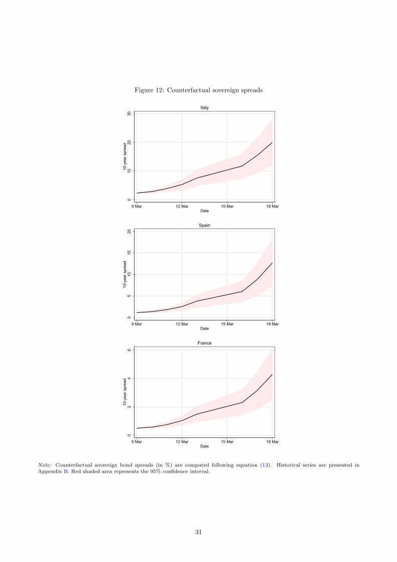
Figure 12: Counterfactual sovereign spreads

010

2030

10-y

ear s

prea

d

9 Mar 12 Mar 15 Mar 18 MarDate

Italy

05

1015

2010

-yea

r spr

ead

9 Mar 12 Mar 15 Mar 18 MarDate

Spain

02

46

10-y

ear s

prea

d

9 Mar 12 Mar 15 Mar 18 MarDate

France

Note: Counterfactual sovereign bond spreads (in %) are computed following equation (13). Historical series are presented inAppendix B. Red shaded area represents the 95% confidence interval.

31

during the 2010-12 sovereign debt crisis in Europe.

This conclusion rests on the study of sovereign debt markets during the first few months of the sanitary

crisis and is corroborated by the extension of our analysis to stock markets. The duration of this sanitary crisis

is still uncertain given the state of medical knowledge. However, its economic consequences on public finances

will certainly be more lasting and raise additional challenges for public decision-makers, in Europe and around

the world, in managing the public debt induced by the COVID crisis.

32

References

Afonso, A., Arghyrou, M. G., Bagdatoglou, G., and Kontonikas, A. (2015a). On the time-varying relationship

between emu sovereign spreads and their determinants. Economic Modelling, 44:363–371.

Afonso, A., Arghyrou, M. G., Gadea, M. D., and Kontonikas, A. (2018). “whatever it takes” to resolve

the european sovereign debt crisis? bond pricing regime switches and monetary policy effects. Journal of

International Money and Finance, 86:1–30.

Afonso, A., Arghyrou, M. G., and Kontonikas, A. (2015b). The determinants of sovereign bond yield spreads

in the emu. European Central Bank Working Paper Series No 1781.

Afonso, A. and Jalles, J. T. (2019). Quantitative easing and sovereign yield spreads: Euro-area time-varying

evidence. Journal of International Financial Markets, Institutions and Money, 58:208–224.

Aizenman, J., Hutchison, M., and Jinjarak, Y. (2013). What is the risk of european sovereign debt defaults?

fiscal space, cds spreads and market pricing of risk. Journal of International Money and Finance, 34:37–59.

Andries, A. M., Ongena, S., and Sprincean, N. (2020). The covid-19 pandemic and sovereign bond risk. Swiss

Finance Institute Research Paper, (20-42).

Arellano, C., Bai, Y., and Mihalache, G. P. (2020). Deadly debt crises: Covid-19 in emerging markets. Technical

report, National Bureau of Economic Research.

Atkeson, A. (2020). What will be the economic impact of covid-19 in the us? rough estimates of disease

scenarios. Technical report, National Bureau of Economic Research.

Auerbach, A. J. and Gorodnichenko, Y. (2013). Fiscal multipliers in recession and expansion. Fiscal Policy

after the Financial Crisis, page 63.

Augustin, P., Sokolovski, V., Subrahmanyam, M. G., and Tomio, D. (2020). In sickness and in debt: The

covid-19 impact on sovereign credit risk. Available at SSRN 3613432.

Barro, R. J., Ursua, J. F., and Weng, J. (2020). The coronavirus and the great influenza pandemic: Lessons

from the “spanish flu” for the coronavirus’s potential effects on mortality and economic activity. Technical

report, National Bureau of Economic Research.

33

Born, B., Muller, G. J., and Pfeifer, J. (2019). Does austerity pay off? Review of Economics and Statistics,

pages 1–45.

Casiraghi, M., Gaiotti, E., Rodano, L., and Secchi, A. (2016). Ecb unconventional monetary policy and the

italian economy during the sovereign debt crisis. International Journal of Central Banking, 12(2):269–315.

Castelnuovo, E. (2019). Yield curve and financial uncertainty: Evidence based on us data. Australian Economic

Review, 52(3):323–335.

Cavallino, P. and De Fiore, F. (2020). Central banks’ response to covid-19 in advanced economies. Technical

report, Bank for International Settlements.

Cezar, R., Gigout, T., and Tripier, F. (2020). Cross-border investments and uncertainty: Firm-level evidence.

Journal of International Money and Finance, page 102159.

Chow, G. C. (1960). Tests of equality between sets of coefficients in two linear regressions. Econometrica:

Journal of the Econometric Society, pages 591–605.

Cloyne, J. S., Jorda, s., and Taylor, A. M. (2020). Decomposing the fiscal multiplier. Working Paper 26939,

National Bureau of Economic Research.

Costantini, M., Fragetta, M., and Melina, G. (2014). Determinants of sovereign bond yield spreads in the emu:

An optimal currency area perspective. European Economic Review, 70:337–349.

Couppey-Soubeyran, J., Perego, E., and Tripier, F. (2020). European banks and the covid-19 crash test.

Technical report, CEPII Policy Brief 32.

Cox, J., Greenwald, D. L., and Ludvigson, S. C. (2020). What explains the covid-19 stock market? Working

Paper 27784, National Bureau of Economic Research.

Crouzet, N. and Mehrotra, N. R. (2020). Small and large firms over the business cycle. American Economic

Review, 110(11):3549–3601.

Davis, S. J., Liu, D., and Sheng, X. S. (2021). Stock prices, lockdowns, and economic activity in the time of

coronavirus. Working Paper 28320, National Bureau of Economic Research.

De Pooter, M., Martin, R. F., and Pruitt, S. (2018). The liquidity effects of official bond market intervention.

Journal of Financial and Quantitative Analysis, 53(1):243–268.

34

Delatte, A.-L., Fouquau, J., and Portes, R. (2017). Regime-dependent sovereign risk pricing during the euro

crisis. Review of Finance, 21(1):363–385.

Delatte, A.-L. and Guillaume, A. (2020). Covid 19: a new challenge for the emu. CEPR Discussion Paper,

DP14848.

ECB (2020a). The covid-19 crisis and its implications for fiscal policies. ECB Monthly Bulletin June.

ECB (2020b). Overview. ECB Financial Stability Review, November.

Eichenbaum, M. S., Rebelo, S., and Trabandt, M. (2020). The macroeconomics of epidemics. Technical report,

National Bureau of Economic Research.

Eser, F. and Schwaab, B. (2016). Evaluating the impact of unconventional monetary policy measures: Empirical

evidence from the ecb’s securities markets programme. Journal of Financial Economics, 119(1):147–167.

Falagiarda, M. and Reitz, S. (2015). Announcements of ecb unconventional programs: Implications for the

sovereign spreads of stressed euro area countries. Journal of International Money and Finance, 53:276–295.

Favara, G. and Imbs, J. (2015). Credit supply and the price of housing. American Economic Review, 105(3):958–

92.

Favero, C. and Missale, A. (2012). Sovereign spreads in the eurozone: which prospects for a eurobond? Economic

Policy, 27(70):231–273.

Fratzscher, M., Duca, M. L., and Straub, R. (2016). Ecb unconventional monetary policy: Market impact and

international spillovers. IMF Economic Review, 64(1):36–74.

Georgoutsos, D. A. and Migiakis, P. M. (2013). Heterogeneity of the determinants of euro-area sovereign bond

spreads; what does it tell us about financial stability? Journal of Banking & Finance, 37(11):4650–4664.

Ghysels, E., Idier, J., Manganelli, S., and Vergote, O. (2017). A high-frequency assessment of the ecb securities

markets programme. Journal of the European Economic Association, 15(1):218–243.

Gibson, H. D., Hall, S. G., and Tavlas, G. S. (2016). The effectiveness of the ecb’s asset purchase programs of

2009 to 2012. Journal of Macroeconomics, 47:45–57.

Guerrieri, V., Lorenzoni, G., Straub, L., and Werning, I. (2020). Macroeconomic implications of covid-19: Can

negative supply shocks cause demand shortages? Technical report, National Bureau of Economic Research.

35

Herbst, E. P. and Johannsen, B. K. (2020). Bias in local projections. Finance and Economics Discussion Series,

2020-010.

Jager, J. and Grigoriadis, T. (2017). The effectiveness of the ecb’s unconventional monetary policy: Comparative

evidence from crisis and non-crisis euro-area countries. Journal of International Money and Finance, 78:21–43.

Jorda, O. (2005). Estimation and inference of impulse responses by local projections. American economic

review, 95(1):161–182.

Jorda, O., Schularick, M., and Taylor, A. M. (2013). When credit bites back. Journal of Money, Credit and

Banking, 45(s2):3–28.

Jorda, O., Schularick, M., and Taylor, A. M. (2015). Leveraged bubbles. Journal of Monetary Economics,

76:S1–S20.

Jorda, O., Schularick, M., and Taylor, A. M. (2016). The great mortgaging: housing finance, crises and business

cycles. Economic policy, 31(85):107–152.

Jorda, O., Schularick, M., and Taylor, A. M. (2020a). The effects of quasi-random monetary experiments.

Journal of Monetary Economics, 112:22–40.

Jorda, O., Singh, S. R., and Taylor, A. M. (2020b). Longer-run economic consequences of pandemics. Technical

report, National Bureau of Economic Research.

Jorda, O. and Taylor, A. M. (2016). The time for austerity: estimating the average treatment effect of fiscal

policy. The Economic Journal, 126(590):219–255.

Kilponen, J., Laakkonen, H., and Vilmunen, J. (2015). Sovereign risk, european crisis resolution policies and

bond yields. International Journal of Central Banking, 11(2):285–323.

Klose, J. and Tillmann, P. (2020). Covid-19 and financial markets: A panel analysis for european countries.

Krishnamurthy, A., Nagel, S., and Vissing-Jorgensen, A. (2018). Ecb policies involving government bond

purchases: Impact and channels. Review of Finance, 22(1):1–44.

Lhuissier, S. and Nguyen, B. (2021). The dynamic effects of the ecb’s asset purchases: a survey-based identifi-

cation. Technical report, Banque de France WP 806.

36

Manganelli, S. and Wolswijk, G. (2009). What drives spreads in the euro area government bond market?

Economic Policy, 24(58):191–240.

Pacicco, F., Vena, L., and Venegoni, A. (2019). Market reactions to ecb policy innovations: A cross-country

analysis. Journal of International Money and Finance, 91:126–137.

Ramey, V. A. and Zubairy, S. (2018). Government spending multipliers in good times and in bad: evidence

from us historical data. Journal of Political Economy, 126(2):850–901.

Schularick, M. and Steffen, S. (2020). A protective shield for europe’s banks. Technical report, mimeo.

Swanson, E. T. (2020). Measuring the effects of federal reserve forward guidance and asset purchases on financial

markets. Journal of Monetary Economics, forthcoming.

Szczerbowicz, U. (2015). The ecb unconventional monetary policies: have they lowered market borrowing costs

for banks and governments? International Journal of Central Banking, 11(4):91–127.

Tenreyro, S. and Thwaites, G. (2016). Pushing on a string: Us monetary policy is less powerful in recessions.

American Economic Journal: Macroeconomics, 8(4):43–74.

Tillmann, P. (2020). Monetary policy uncertainty and the response of the yield curve to policy shocks. Journal

of Money, Credit and Banking, 52(4):803–833.

Trebesch, C. and Zettelmeyer, J. (2018). Ecb interventions in distressed sovereign debt markets: The case of

greek bonds. IMF Economic Review, 66(2):287–332.

37

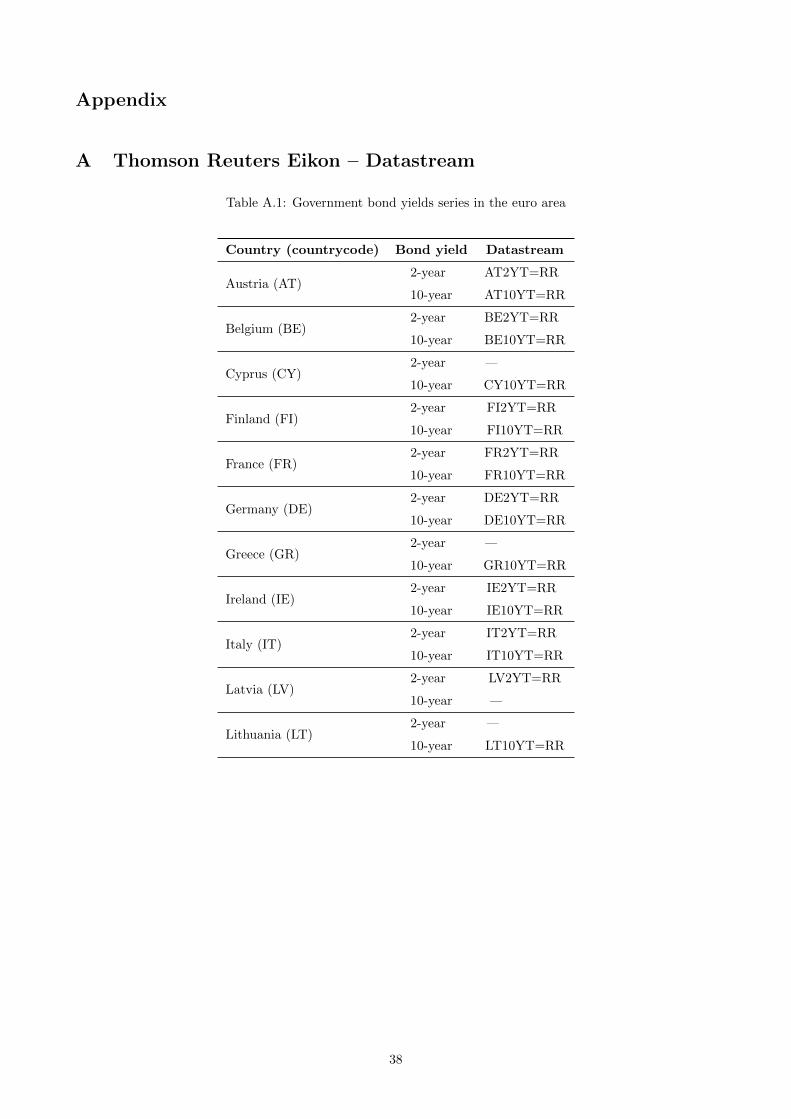
Appendix

A Thomson Reuters Eikon – Datastream

Table A.1: Government bond yields series in the euro area

Country (countrycode) Bond yield Datastream

Austria (AT)2-year

10-year

AT2YT=RR

AT10YT=RR

Belgium (BE)2-year

10-year

BE2YT=RR

BE10YT=RR

Cyprus (CY)2-year

10-year

—

CY10YT=RR

Finland (FI)2-year

10-year

FI2YT=RR

FI10YT=RR

France (FR)2-year

10-year

FR2YT=RR

FR10YT=RR

Germany (DE)2-year

10-year

DE2YT=RR

DE10YT=RR

Greece (GR)2-year

10-year

—

GR10YT=RR

Ireland (IE)2-year

10-year

IE2YT=RR

IE10YT=RR

Italy (IT)2-year

10-year

IT2YT=RR

IT10YT=RR

Latvia (LV)2-year

10-year

LV2YT=RR

—

Lithuania (LT)2-year

10-year

—

LT10YT=RR

38

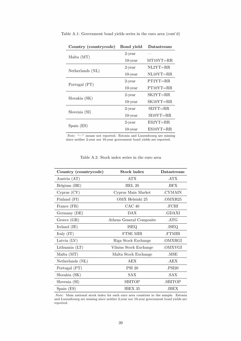
Table A.1: Government bond yields series in the euro area (cont’d)

Country (countrycode) Bond yield Datastream

Malta (MT)2-year

10-year

—

MT10YT=RR

Netherlands (NL)2-year

10-year

NL2YT=RR

NL10YT=RR

Portugal (PT)2-year

10-year

PT2YT=RR

PT10YT=RR

Slovakia (SK)2-year

10-year

SK2YT=RR

SK10YT=RR

Slovenia (SI)2-year

10-year

SI2YT=RR

SI10YT=RR

Spain (ES)2-year

10-year

ES2YT=RR

ES10YT=RR

Note: “—” means not reported. Estonia and Luxembourg are missingsince neither 2-year nor 10-year government bond yields are reported.

Table A.2: Stock index series in the euro area

Country (countrycode) Stock index Datastream

Austria (AT) ATX .ATX

Belgium (BE) BEL 20 .BFX

Cyprus (CY) Cyprus Main Market .CYMAIN

Finland (FI) OMX Helsinki 25 .OMXH25

France (FR) CAC 40 .FCHI

Germany (DE) DAX .GDAXI

Greece (GR) Athens General Composite .ATG

Ireland (IE) ISEQ .ISEQ

Italy (IT) FTSE MIB .FTMIB

Latvia (LV) Riga Stock Exchange .OMXRGI

Lithuania (LT) Vilnius Stock Exchange .OMXVGI

Malta (MT) Malta Stock Exchange .MSE

Netherlands (NL) AEX .AEX

Portugal (PT) PSI 20 .PSI20

Slovakia (SK) SAX .SAX

Slovenia (SI) SBITOP .SBITOP

Spain (ES) IBEX 35 .IBEX

Note: Main national stock index for each euro area countries in the sample. Estoniaand Luxembourg are missing since neither 2-year nor 10-year government bond yields arereported.

39

B Figures: Raw data

Figure B.1: Total number of COVID-19 cases0

500

1000

1500

2000

Jan Mar May

Austria

010

0020

0030

0040

0050

00

Jan Mar May

Belgium

020

040

060

080

010

00

Jan Mar May

Cyprus

050

010

0015

00

Jan Mar May

Finland

050

010

0015

0020

0025

00

Jan Mar May

France

010

020

030

0

Jan Mar May

Greece0

1000

2000

3000

4000

5000

Jan Mar May

Ireland

010

0020

0030

0040

00Jan Mar May

Italy

020

040

060

0

Jan Mar May

Latvia

020

040

060

0

Jan Mar May

Lithuania

050

010

0015

00

Jan Mar May

Malta

010

0020

0030

00

Jan Mar May

Netherlands

010

0020

0030

00

Jan Mar May

Portugal

010

020

030

0

Jan Mar May

Slovakia

020

040

060

080

0

Jan Mar May

Slovenia

010

0020

0030

0040

0050

00

Jan Mar May

Spain

Note: Total COVID-19 confirmed cases are reported as the number of cases per million people. Sources: European Centre forDisease Prevention and Control (ECDC)

41

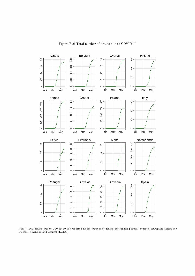
Figure B.2: Total number of deaths due to COVID-190

2040

6080

Jan Mar May

Austria

020

040

060

080

0

Jan Mar May

Belgium

05

1015

20

Jan Mar May

Cyprus

020

4060

Jan Mar May

Finland

010

020

030

040

0

Jan Mar May

France

05

1015

20

Jan Mar May

Greece0

100

200

300

400

Jan Mar May

Ireland

020

040

060

0Jan Mar May

Italy

05

1015

Jan Mar May

Latvia

05

1015

2025

Jan Mar May

Lithuania

05

1015

Jan Mar May

Malta

010

020

030

040

0

Jan Mar May

Netherlands

050

100

150

Jan Mar May

Portugal

01

23

45

Jan Mar May

Slovakia

010

2030

4050

Jan Mar May

Slovenia

020

040

060

0

Jan Mar May

Spain

Note: Total deaths due to COVID-19 are reported as the number of deaths per million people. Sources: European Centre forDisease Prevention and Control (ECDC)

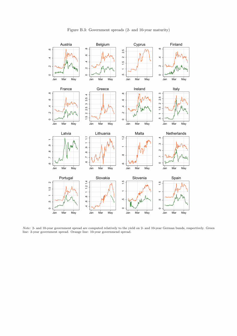
Figure B.3: Government spreads (2- and 10-year maturity)

0.2

.4.6

Jan Mar May

Austria

0.2

.4.6

.8

Jan Mar May

Belgium

.51

1.5

22.

5

Jan Mar May

Cyprus

0.2

.4.6

Jan Mar May

Finland0

.2.4

.6.8

Jan Mar May

France1.

52

2.5

33.

54

Jan Mar May

Greece

0.2

.4.6

.8Jan Mar May

Ireland

.51

1.5

22.

53

Jan Mar May

Italy

.6.7

.8.9

1

Jan Mar May

Latvia

.6.7

.8.9

11.

1

Jan Mar May

Lithuania

.6.8

11.

2

Jan Mar May

Malta

0.1

.2.3

.4

Jan Mar May

Netherlands

0.5

11.

52

Jan Mar May

Portugal

.4.6

.81

1.2

1.4

Jan Mar May

Slovakia

0.5

11.

5

Jan Mar May

Slovenia

0.5

11.

5

Jan Mar May

Spain

Note: 2- and 10-year government spread are computed relatively to the yield on 2- and 10-year German bunds, respectively. Greenline: 2-year government spread. Orange line: 10-year governmend spread.

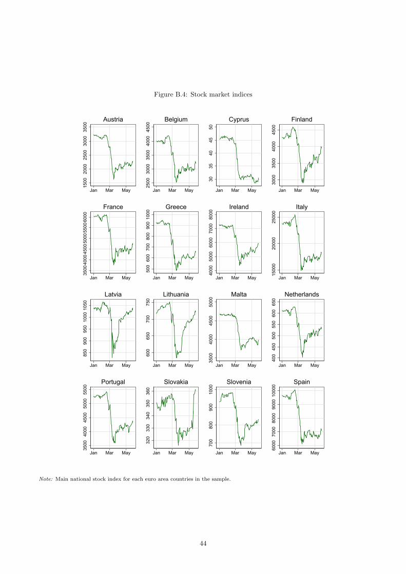
Figure B.4: Stock market indices

1500

2000

2500

3000

3500

Jan Mar May

Austria

2500

3000

3500

4000

4500

Jan Mar May

Belgium

3035

4045

50

Jan Mar May

Cyprus

3000

3500

4000

4500

Jan Mar May

Finland

3500

4000

4500

5000

5500

6000

Jan Mar May

France

500

600

700

800

900

1000

Jan Mar May

Greece40

0050

0060

0070

0080

00

Jan Mar May

Ireland

1500

020

000

2500

0Jan Mar May

Italy

850

900

950

1000

1050

Jan Mar May

Latvia

600

650

700

750

Jan Mar May

Lithuania

3500

4000

4500

5000

Jan Mar May

Malta

400

450

500

550

600

650

Jan Mar May

Netherlands

3500

4000

4500

5000

5500

Jan Mar May

Portugal

320

330

340

350

360

Jan Mar May

Slovakia

700

800

900

1000

Jan Mar May

Slovenia

6000

7000

8000

9000

1000

0

Jan Mar May

Spain

Note: Main national stock index for each euro area countries in the sample.

44

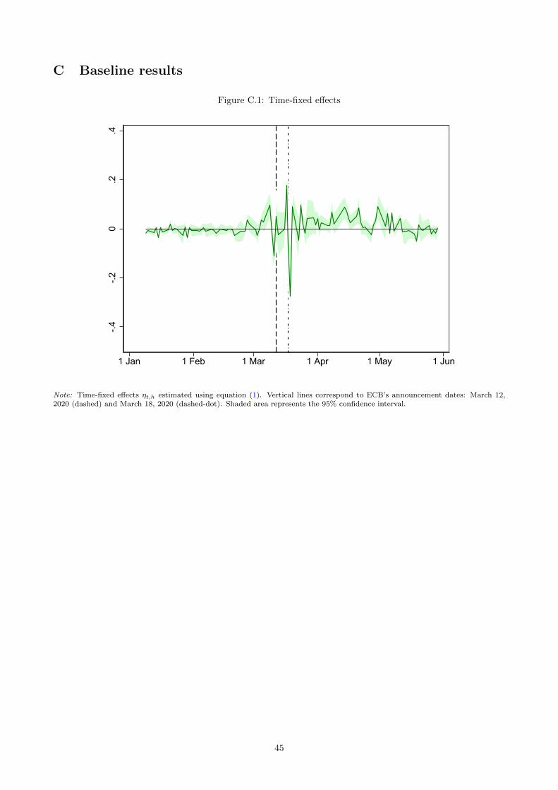
C Baseline results

Figure C.1: Time-fixed effects-.4

-.20

.2.4

1 Jan 1 Feb 1 Mar 1 Apr 1 May 1 Jun

Note: Time-fixed effects ηt,h estimated using equation (1). Vertical lines correspond to ECB’s announcement dates: March 12,2020 (dashed) and March 18, 2020 (dashed-dot). Shaded area represents the 95% confidence interval.

45

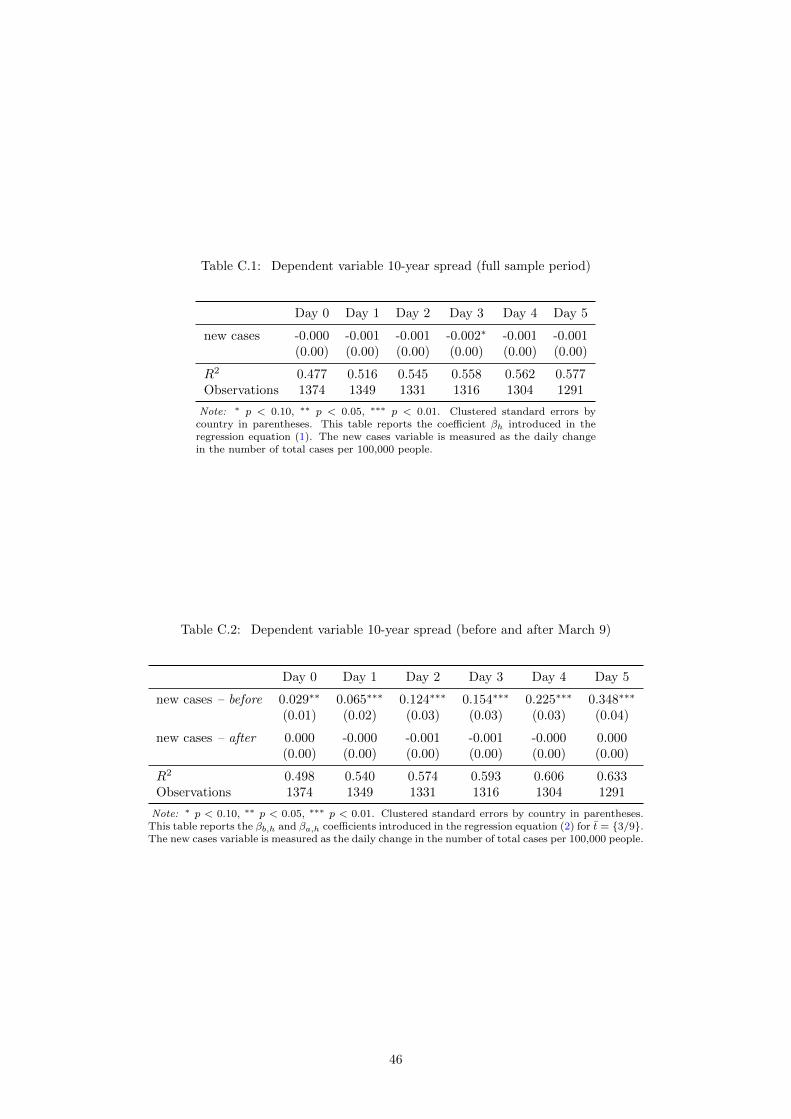
Table C.1: Dependent variable 10-year spread (full sample period)

Day 0 Day 1 Day 2 Day 3 Day 4 Day 5

new cases -0.000 -0.001 -0.001 -0.002∗ -0.001 -0.001(0.00) (0.00) (0.00) (0.00) (0.00) (0.00)

R2 0.477 0.516 0.545 0.558 0.562 0.577Observations 1374 1349 1331 1316 1304 1291

Note: ∗ p < 0.10, ∗∗ p < 0.05, ∗∗∗ p < 0.01. Clustered standard errors bycountry in parentheses. This table reports the coefficient βh introduced in theregression equation (1). The new cases variable is measured as the daily changein the number of total cases per 100,000 people.

Table C.2: Dependent variable 10-year spread (before and after March 9)

Day 0 Day 1 Day 2 Day 3 Day 4 Day 5

new cases – before 0.029∗∗ 0.065∗∗∗ 0.124∗∗∗ 0.154∗∗∗ 0.225∗∗∗ 0.348∗∗∗

(0.01) (0.02) (0.03) (0.03) (0.03) (0.04)

new cases – after 0.000 -0.000 -0.001 -0.001 -0.000 0.000(0.00) (0.00) (0.00) (0.00) (0.00) (0.00)

R2 0.498 0.540 0.574 0.593 0.606 0.633Observations 1374 1349 1331 1316 1304 1291

Note: ∗ p < 0.10, ∗∗ p < 0.05, ∗∗∗ p < 0.01. Clustered standard errors by country in parentheses.This table reports the βb,h and βa,h coefficients introduced in the regression equation (2) for t = {3/9}.The new cases variable is measured as the daily change in the number of total cases per 100,000 people.

46

D Robustness: Alternative variables

Figure D.1: Impulse responses of 2-year government bond spreads to new COVID-19 cases in the euro area

0.2

.4.6

.8

0 1 2 3 4 5Days

5-9 March10-16 March17-25 March

Note: Impulse responses are computed following equation (3). Impulse response coefficients βb,h are estimated before splittingdates: t ∈ {3/5, ..., 3/9} in red, t ∈ {3/10, ..., 3/16} in blue, and t ∈ {3/17, ..., 3/25} in green. Shaded area represents the 95%confidence interval for each coefficient.

47

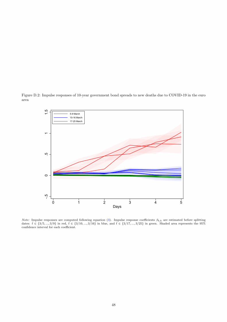
Figure D.2: Impulse responses of 10-year government bond spreads to new deaths due to COVID-19 in the euroarea

-.50

.51

1.5

0 1 2 3 4 5Days

5-9 March10-16 March17-25 March

Note: Impulse responses are computed following equation (3). Impulse response coefficients βb,h are estimated before splittingdates: t ∈ {3/5, ..., 3/9} in red, t ∈ {3/10, ..., 3/16} in blue, and t ∈ {3/17, ..., 3/25} in green. Shaded area represents the 95%confidence interval for each coefficient.

48

Figure D.3: Impulse responses of 10-year government bond spreads to new COVID-19 cases (3-day rollingaverage) in the euro area

-.20

.2.4

.6

0 1 2 3 4 5Days

5-10 March11-16 March17-25 March

Note: Impulse responses are computed following equation (3). Impulse response coefficients βb,h are estimated before splittingdates: t ∈ {3/5, ..., 3/10} in red, t ∈ {3/11, ..., 3/16} in blue, and t ∈ {3/17, ..., 3/25} in green. Shaded area represents the 95%confidence interval for each coefficient.

49

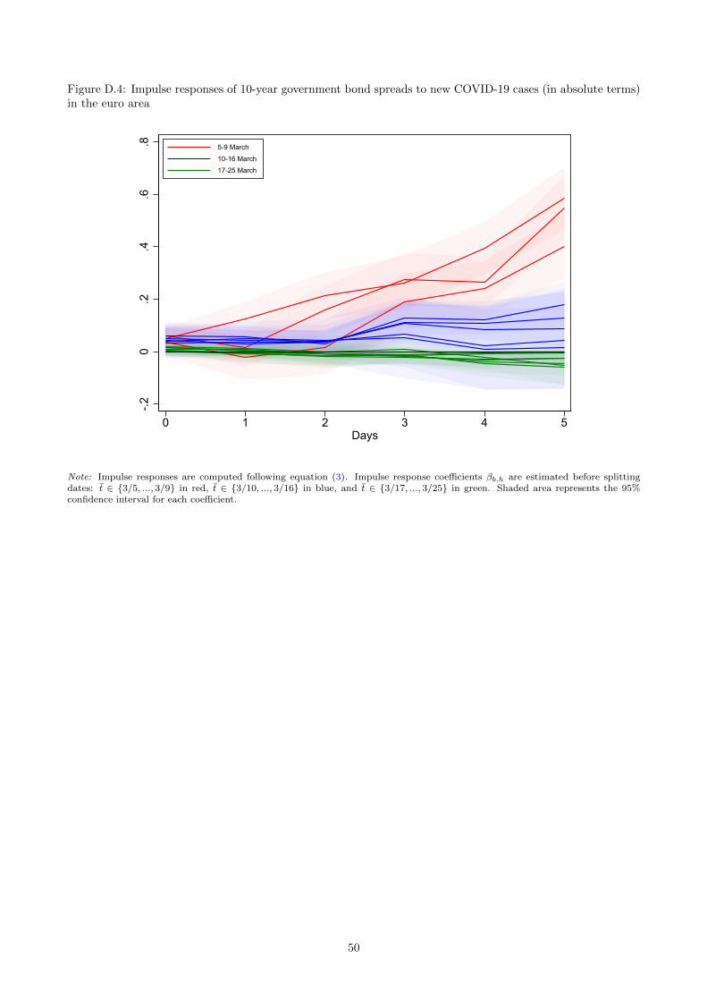
Figure D.4: Impulse responses of 10-year government bond spreads to new COVID-19 cases (in absolute terms)in the euro area

-.20

.2.4

.6.8

0 1 2 3 4 5Days

5-9 March10-16 March17-25 March

Note: Impulse responses are computed following equation (3). Impulse response coefficients βb,h are estimated before splittingdates: t ∈ {3/5, ..., 3/9} in red, t ∈ {3/10, ..., 3/16} in blue, and t ∈ {3/17, ..., 3/25} in green. Shaded area represents the 95%confidence interval for each coefficient.

50

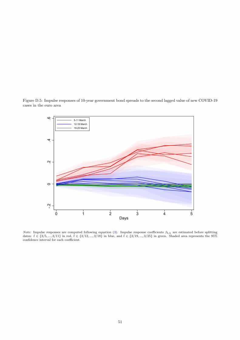
Figure D.5: Impulse responses of 10-year government bond spreads to the second lagged value of new COVID-19cases in the euro area

-.20

.2.4

.6

0 1 2 3 4 5Days

5-11 March12-18 March19-25 March

Note: Impulse responses are computed following equation (3). Impulse response coefficients βb,h are estimated before splittingdates: t ∈ {3/5, ..., 3/11} in red, t ∈ {3/12, ..., 3/18} in blue, and t ∈ {3/19, ..., 3/25} in green. Shaded area represents the 95%confidence interval for each coefficient.

51

Figure D.6: Impulse responses of 10-year government bond spreads to the growth rate of total COVID-19 casesin the euro area

-.15

-.1-.0

50

.05

0 1 2 3 4 5Days

5-9 March10-16 March17-25 March

Note: Impulse responses are computed following equation (3). Impulse response coefficients βb,h are estimated before splittingdates: t ∈ {3/5, ..., 3/9} in red, t ∈ {3/10, ..., 3/16} in blue, and t ∈ {3/17, ..., 3/25} in green. Shaded area represents the 95%confidence interval for each coefficient.

52

Table D.1: Chow test (p-values, using 2-year maturity)

Horizonh=0 h=1 h=2 h=3 h=4 h=5

March 5 0.02 0.26 0.10 0.00 0.00 0.00March 6 0.01 0.08 0.00 0.00 0.00 0.00March 9 0.01 0.00 0.00 0.00 0.00 0.00March 10 0.00 0.00 0.01 0.01 0.01 0.00March 11 0.00 0.04 0.01 0.01 0.01 0.00March 12 0.02 0.11 0.06 0.03 0.02 0.00March 13 0.03 0.12 0.03 0.02 0.01 0.01March 16 0.10 0.09 0.03 0.02 0.02 0.01March 17 0.07 0.05 0.02 0.03 0.01 0.02March 18 0.07 0.04 0.03 0.05 0.45 0.24March 19 0.07 0.11 0.07 0.07 0.37 0.27March 20 0.18 0.18 0.10 0.12 0.54 0.56March 23 0.21 0.18 0.14 0.17 0.78 0.51March 24 0.19 0.28 0.19 0.49 0.64 0.51March 25 0.28 0.36 0.30 0.66 0.70 0.53

Note: p-values of Chow statistics from the test.

53

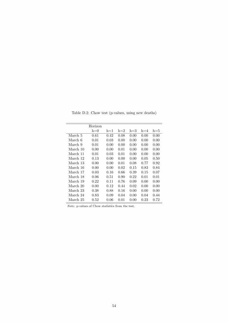
Table D.2: Chow test (p-values, using new deaths)

Horizonh=0 h=1 h=2 h=3 h=4 h=5

March 5 0.61 0.42 0.08 0.00 0.00 0.00March 6 0.01 0.03 0.00 0.00 0.00 0.00March 9 0.01 0.00 0.00 0.00 0.00 0.00March 10 0.00 0.00 0.01 0.00 0.00 0.00March 11 0.01 0.03 0.01 0.00 0.00 0.00March 12 0.13 0.00 0.00 0.00 0.05 0.50March 13 0.00 0.00 0.01 0.08 0.77 0.92March 16 0.00 0.00 0.02 0.15 0.83 0.84March 17 0.03 0.16 0.66 0.39 0.15 0.07March 18 0.06 0.51 0.90 0.22 0.01 0.01March 19 0.22 0.11 0.76 0.09 0.00 0.00March 20 0.00 0.12 0.44 0.02 0.00 0.00March 23 0.38 0.88 0.16 0.00 0.00 0.00March 24 0.83 0.09 0.04 0.00 0.04 0.44March 25 0.52 0.06 0.01 0.00 0.23 0.72

Note: p-values of Chow statistics from the test.

54

Table D.3: Chow test (p-values, using new cases (3-day rolling average)

Horizonh=0 h=1 h=2 h=3 h=4 h=5

March 5 0.97 0.58 0.11 0.00 0.00 0.00March 6 0.12 0.13 0.00 0.00 0.00 0.00March 9 0.11 0.00 0.00 0.00 0.00 0.00March 10 0.08 0.04 0.09 0.01 0.00 0.00March 11 0.56 0.95 0.16 0.06 0.02 0.17March 12 0.58 0.30 0.14 0.14 0.37 0.98March 13 0.50 0.26 0.27 0.54 1.00 0.77March 16 0.50 0.48 0.64 0.92 0.86 0.67March 17 0.73 0.91 0.86 0.92 0.54 0.28March 18 0.98 0.71 0.64 0.31 0.15 0.12March 19 0.45 0.56 0.23 0.08 0.06 0.06March 20 0.70 0.50 0.17 0.08 0.07 0.10March 23 0.41 0.30 0.16 0.07 0.04 0.07March 24 0.60 0.26 0.18 0.05 0.07 0.34March 25 0.98 0.59 0.33 0.25 0.75 0.37

Note: p-values of Chow statistics from the test.

55

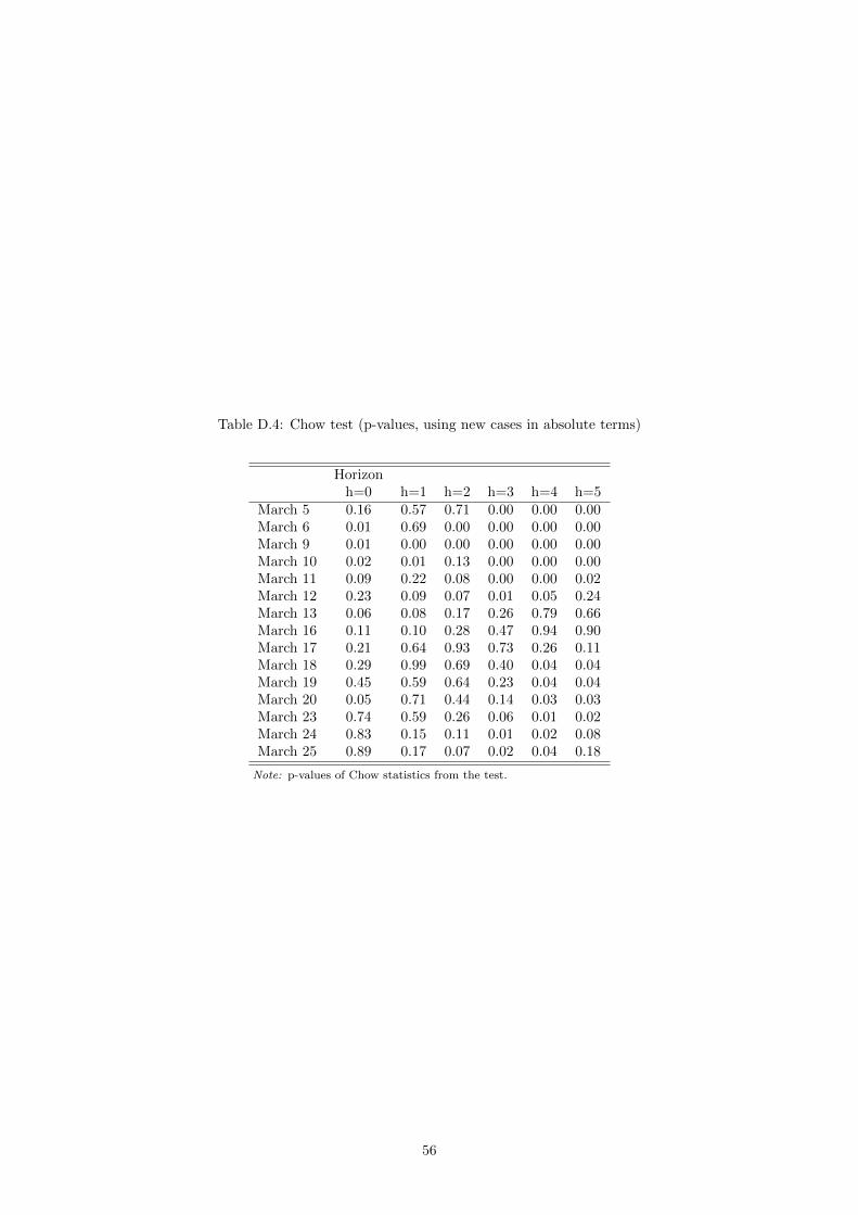
Table D.4: Chow test (p-values, using new cases in absolute terms)

Horizonh=0 h=1 h=2 h=3 h=4 h=5

March 5 0.16 0.57 0.71 0.00 0.00 0.00March 6 0.01 0.69 0.00 0.00 0.00 0.00March 9 0.01 0.00 0.00 0.00 0.00 0.00March 10 0.02 0.01 0.13 0.00 0.00 0.00March 11 0.09 0.22 0.08 0.00 0.00 0.02March 12 0.23 0.09 0.07 0.01 0.05 0.24March 13 0.06 0.08 0.17 0.26 0.79 0.66March 16 0.11 0.10 0.28 0.47 0.94 0.90March 17 0.21 0.64 0.93 0.73 0.26 0.11March 18 0.29 0.99 0.69 0.40 0.04 0.04March 19 0.45 0.59 0.64 0.23 0.04 0.04March 20 0.05 0.71 0.44 0.14 0.03 0.03March 23 0.74 0.59 0.26 0.06 0.01 0.02March 24 0.83 0.15 0.11 0.01 0.02 0.08March 25 0.89 0.17 0.07 0.02 0.04 0.18

Note: p-values of Chow statistics from the test.

56

Table D.5: Chow test (p-values, second lagged value of new cases)

Horizonh=0 h=1 h=2 h=3 h=4 h=5

March 5 0.01 0.00 0.00 0.00 0.00 0.00March 6 0.00 0.00 0.00 0.00 0.00 0.00March 9 0.00 0.00 0.00 0.00 0.00 0.00March 10 0.00 0.00 0.00 0.00 0.00 0.00March 11 0.17 0.05 0.00 0.00 0.00 0.00March 12 0.01 0.01 0.03 0.03 0.55 0.69March 13 0.54 0.01 0.07 0.21 1.00 0.52March 16 0.55 0.18 0.49 0.72 0.87 0.49March 17 0.73 0.48 0.87 0.82 0.72 0.31March 18 0.98 0.84 0.99 0.82 0.34 0.18March 19 0.11 0.34 0.04 0.07 0.07 0.05March 20 0.46 0.22 0.03 0.06 0.07 0.07March 23 0.13 0.06 0.06 0.05 0.10 0.07March 24 0.12 0.12 0.08 0.03 0.13 0.17March 25 0.19 0.41 0.16 0.11 0.53 0.75

Note: p-values of Chow statistics from the test.

57

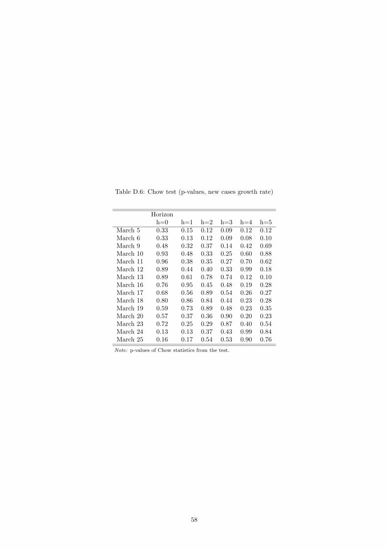
Table D.6: Chow test (p-values, new cases growth rate)

Horizonh=0 h=1 h=2 h=3 h=4 h=5

March 5 0.33 0.15 0.12 0.09 0.12 0.12March 6 0.33 0.13 0.12 0.09 0.08 0.10March 9 0.48 0.32 0.37 0.14 0.42 0.69March 10 0.93 0.48 0.33 0.25 0.60 0.88March 11 0.96 0.38 0.35 0.27 0.70 0.62March 12 0.89 0.44 0.40 0.33 0.99 0.18March 13 0.89 0.61 0.78 0.74 0.12 0.10March 16 0.76 0.95 0.45 0.48 0.19 0.28March 17 0.68 0.56 0.89 0.54 0.26 0.27March 18 0.80 0.86 0.84 0.44 0.23 0.28March 19 0.59 0.73 0.89 0.48 0.23 0.35March 20 0.57 0.37 0.36 0.90 0.20 0.23March 23 0.72 0.25 0.29 0.87 0.40 0.54March 24 0.13 0.13 0.37 0.43 0.99 0.84March 25 0.16 0.17 0.54 0.53 0.90 0.76

Note: p-values of Chow statistics from the test.

58

E Robustness: Controlling for the shape of the pandemic

59

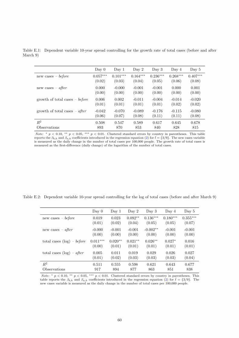
Table E.1: Dependent variable 10-year spread controlling for the growth rate of total cases (before and afterMarch 9)

Day 0 Day 1 Day 2 Day 3 Day 4 Day 5

new cases – before 0.057∗∗∗ 0.101∗∗∗ 0.164∗∗∗ 0.236∗∗∗ 0.268∗∗∗ 0.407∗∗∗

(0.02) (0.03) (0.04) (0.05) (0.06) (0.08)

new cases – after 0.000 -0.000 -0.001 -0.001 0.000 0.001(0.00) (0.00) (0.00) (0.00) (0.00) (0.00)

growth of total cases – before 0.006 0.002 -0.011 -0.004 -0.014 -0.020(0.01) (0.01) (0.01) (0.01) (0.02) (0.02)

growth of total cases – after -0.042 -0.070 -0.089 -0.176 -0.115 -0.080(0.06) (0.07) (0.08) (0.11) (0.11) (0.08)

R2 0.508 0.547 0.589 0.617 0.645 0.678Observations 893 870 853 840 828 815

Note: ∗ p < 0.10, ∗∗ p < 0.05, ∗∗∗ p < 0.01. Clustered standard errors by country in parentheses. This tablereports the βb,h and βa,h coefficients introduced in the regression equation (2) for t = {3/9}. The new cases variableis measured as the daily change in the number of total cases per 100,000 people. The growth rate of total cases ismeasured as the first-difference (daily change) of the logarithm of the number of total cases.

Table E.2: Dependent variable 10-year spread controlling for the log of total cases (before and after March 9)

Day 0 Day 1 Day 2 Day 3 Day 4 Day 5

new cases – before 0.019 0.023 0.092∗∗ 0.136∗∗∗ 0.180∗∗∗ 0.355∗∗∗

(0.01) (0.02) (0.04) (0.05) (0.05) (0.07)

new cases – after -0.000 -0.001 -0.001 -0.002∗∗ -0.001 -0.001(0.00) (0.00) (0.00) (0.00) (0.00) (0.00)

total cases (log) – before 0.011∗∗∗ 0.020∗∗ 0.021∗∗ 0.026∗∗ 0.027∗ 0.016(0.00) (0.01) (0.01) (0.01) (0.01) (0.01)

total cases (log) – after 0.005 0.011 0.019 0.029 0.026 0.027(0.01) (0.02) (0.03) (0.03) (0.03) (0.04)

R2 0.511 0.555 0.598 0.621 0.643 0.677Observations 917 894 877 863 851 838

Note: ∗ p < 0.10, ∗∗ p < 0.05, ∗∗∗ p < 0.01. Clustered standard errors by country in parentheses. Thistable reports the βb,h and βa,h coefficients introduced in the regression equation (2) for t = {3/9}. Thenew cases variable is measured as the daily change in the number of total cases per 100,000 people.

60

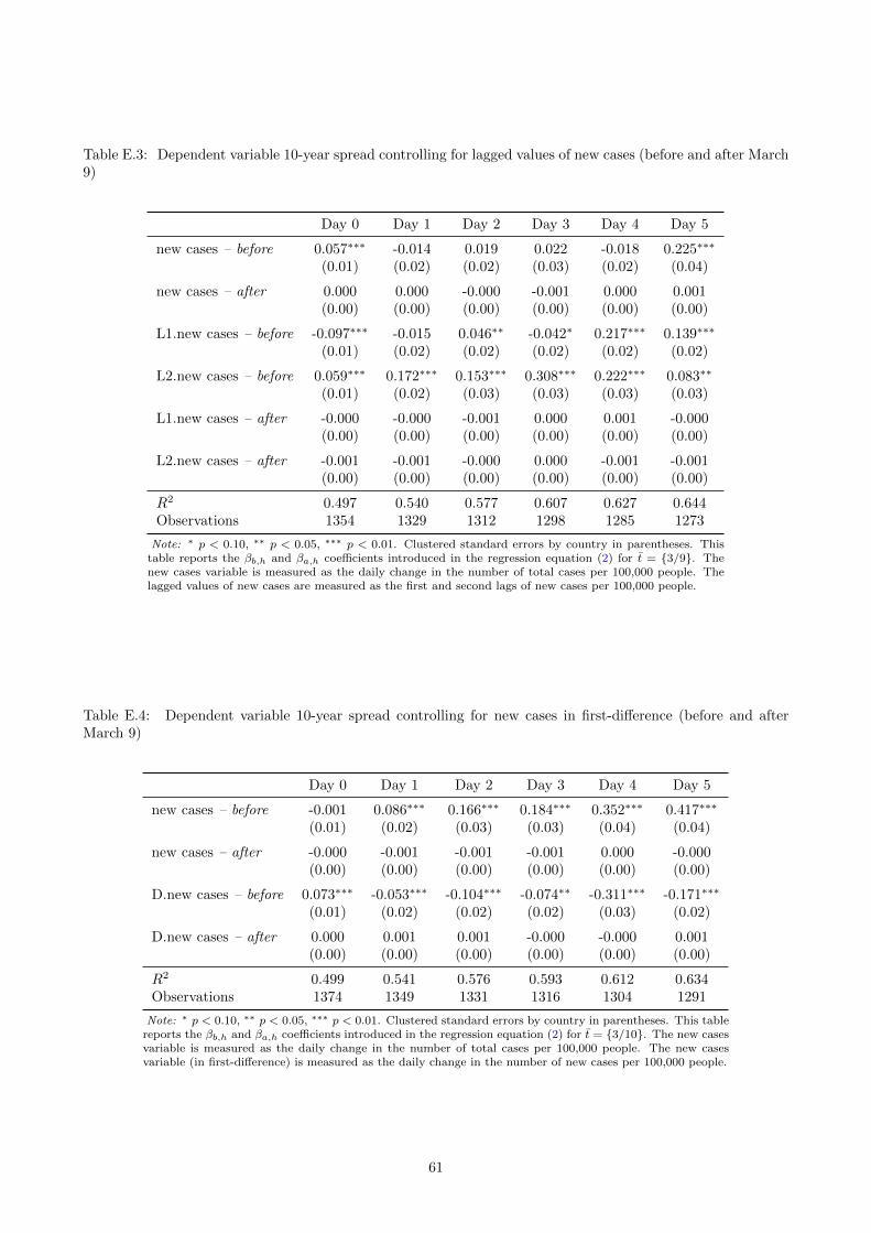
Table E.3: Dependent variable 10-year spread controlling for lagged values of new cases (before and after March9)

Day 0 Day 1 Day 2 Day 3 Day 4 Day 5

new cases – before 0.057∗∗∗ -0.014 0.019 0.022 -0.018 0.225∗∗∗

(0.01) (0.02) (0.02) (0.03) (0.02) (0.04)

new cases – after 0.000 0.000 -0.000 -0.001 0.000 0.001(0.00) (0.00) (0.00) (0.00) (0.00) (0.00)

L1.new cases – before -0.097∗∗∗ -0.015 0.046∗∗ -0.042∗ 0.217∗∗∗ 0.139∗∗∗

(0.01) (0.02) (0.02) (0.02) (0.02) (0.02)

L2.new cases – before 0.059∗∗∗ 0.172∗∗∗ 0.153∗∗∗ 0.308∗∗∗ 0.222∗∗∗ 0.083∗∗

(0.01) (0.02) (0.03) (0.03) (0.03) (0.03)

L1.new cases – after -0.000 -0.000 -0.001 0.000 0.001 -0.000(0.00) (0.00) (0.00) (0.00) (0.00) (0.00)

L2.new cases – after -0.001 -0.001 -0.000 0.000 -0.001 -0.001(0.00) (0.00) (0.00) (0.00) (0.00) (0.00)

R2 0.497 0.540 0.577 0.607 0.627 0.644Observations 1354 1329 1312 1298 1285 1273

Note: ∗ p < 0.10, ∗∗ p < 0.05, ∗∗∗ p < 0.01. Clustered standard errors by country in parentheses. Thistable reports the βb,h and βa,h coefficients introduced in the regression equation (2) for t = {3/9}. Thenew cases variable is measured as the daily change in the number of total cases per 100,000 people. Thelagged values of new cases are measured as the first and second lags of new cases per 100,000 people.

Table E.4: Dependent variable 10-year spread controlling for new cases in first-difference (before and afterMarch 9)

Day 0 Day 1 Day 2 Day 3 Day 4 Day 5

new cases – before -0.001 0.086∗∗∗ 0.166∗∗∗ 0.184∗∗∗ 0.352∗∗∗ 0.417∗∗∗

(0.01) (0.02) (0.03) (0.03) (0.04) (0.04)

new cases – after -0.000 -0.001 -0.001 -0.001 0.000 -0.000(0.00) (0.00) (0.00) (0.00) (0.00) (0.00)

D.new cases – before 0.073∗∗∗ -0.053∗∗∗ -0.104∗∗∗ -0.074∗∗ -0.311∗∗∗ -0.171∗∗∗

(0.01) (0.02) (0.02) (0.02) (0.03) (0.02)

D.new cases – after 0.000 0.001 0.001 -0.000 -0.000 0.001(0.00) (0.00) (0.00) (0.00) (0.00) (0.00)

R2 0.499 0.541 0.576 0.593 0.612 0.634Observations 1374 1349 1331 1316 1304 1291

Note: ∗ p < 0.10, ∗∗ p < 0.05, ∗∗∗ p < 0.01. Clustered standard errors by country in parentheses. This tablereports the βb,h and βa,h coefficients introduced in the regression equation (2) for t = {3/10}. The new casesvariable is measured as the daily change in the number of total cases per 100,000 people. The new casesvariable (in first-difference) is measured as the daily change in the number of new cases per 100,000 people.

61

F Robustness: Public debt-to-GDP

Figure F.1: Impulse responses of 10-year government bond spreads to new COVID-19 cases in the euro area

0.1

.2.3

.4.5

0 1 2 3 4 5Horizon h

Before March 9 (high debt/GDP)

-1-.5

0.5

1

0 1 2 3 4 5Horizon h

Before March 9 (low debt/GDP)

Note: Impulse responses are computed following equation (3). Left panel shows coefficient βb,h for countries with a high debt/GDPratio, whereas right panel shows coefficient βb,h for countries with a low debt/GDP ratio. Both panels show response coefficientsestimated before the splitting date. Grey shaded area represents the 95% confidence interval.

62

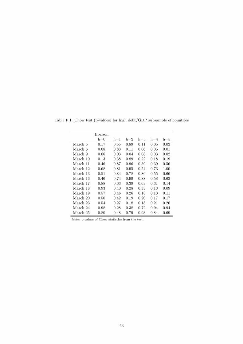
Table F.1: Chow test (p-values) for high debt/GDP subsample of countries

Horizonh=0 h=1 h=2 h=3 h=4 h=5

March 5 0.17 0.55 0.89 0.11 0.05 0.02March 6 0.08 0.83 0.11 0.06 0.05 0.01March 9 0.06 0.03 0.04 0.08 0.03 0.02March 10 0.13 0.38 0.89 0.22 0.18 0.19March 11 0.46 0.87 0.96 0.39 0.39 0.56March 12 0.68 0.81 0.95 0.54 0.73 1.00March 13 0.51 0.84 0.78 0.86 0.55 0.66March 16 0.46 0.74 0.99 0.88 0.58 0.63March 17 0.88 0.63 0.39 0.63 0.31 0.14March 18 0.93 0.40 0.28 0.33 0.13 0.09March 19 0.57 0.46 0.26 0.18 0.13 0.11March 20 0.50 0.42 0.19 0.20 0.17 0.17March 23 0.54 0.27 0.18 0.18 0.21 0.20March 24 0.98 0.28 0.38 0.72 0.94 0.94March 25 0.80 0.48 0.79 0.93 0.84 0.69

Note: p-values of Chow statistics from the test.

63

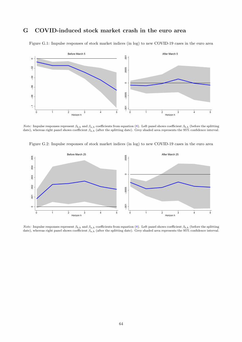
G COVID-induced stock market crash in the euro area

Figure G.1: Impulse responses of stock market indices (in log) to new COVID-19 cases in the euro area

-.1-.0

8-.0

6-.0

4-.0

20

0 1 2 3 4 5Horizon h

Before March 5

-.001

-.000

50

.000

5.0

01

0 1 2 3 4 5Horizon h

After March 5

Note: Impulse responses represent βb,h and βa,h coefficients from equation (8). Left panel shows coefficient βb,h (before the splittingdate), whereas right panel shows coefficient βa,h (after the splitting date). Grey shaded area represents the 95% confidence interval.

Figure G.2: Impulse responses of stock market indices (in log) to new COVID-19 cases in the euro area

0.0

01.0

02.0

03.0

04.0

05

0 1 2 3 4 5Horizon h

Before March 25

-.001

-.000

50

.000

5

0 1 2 3 4 5Horizon h

After March 25

Note: Impulse responses represent βb,h and βa,h coefficients from equation (8). Left panel shows coefficient βb,h (before the splittingdate), whereas right panel shows coefficient βa,h (after the splitting date). Grey shaded area represents the 95% confidence interval.

64

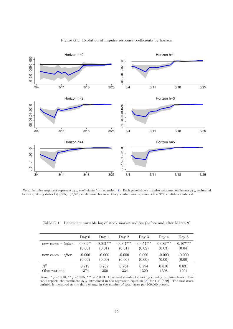
Figure G.3: Evolution of impulse response coefficients by horizon

-.015

-.01-.

005

0.0

05

3/4 3/11 3/18 3/25

Horizon h=0

-.06

-.04

-.02

0

3/4 3/11 3/18 3/25

Horizon h=1

-.08-

.06-

.04-

.02

0

3/4 3/11 3/18 3/25

Horizon h=2

-.1-.0

8-.06

-.04-.

020

3/4 3/11 3/18 3/25

Horizon h=3

-.15

-.1-.0

50

3/4 3/11 3/18 3/25

Horizon h=4

-.2-.1

5-.1

-.05

0

3/4 3/11 3/18 3/25

Horizon h=5

Note: Impulse responses represent βb,h coefficients from equation (8). Each panel shows impulse response coefficients βb,h estimatedbefore splitting dates t ∈ {3/5, ..., 3/25} at different horizon. Grey shaded area represents the 95% confidence interval.

Table G.1: Dependent variable log of stock market indices (before and after March 9)

Day 0 Day 1 Day 2 Day 3 Day 4 Day 5

new cases – before -0.009∗∗ -0.031∗∗∗ -0.047∗∗∗ -0.057∗∗∗ -0.089∗∗∗ -0.107∗∗∗

(0.00) (0.01) (0.01) (0.02) (0.03) (0.04)

new cases – after -0.000 -0.000 -0.000 0.000 -0.000 -0.000(0.00) (0.00) (0.00) (0.00) (0.00) (0.00)

R2 0.719 0.732 0.764 0.794 0.816 0.831Observations 1374 1350 1334 1320 1308 1294

Note: ∗ p < 0.10, ∗∗ p < 0.05, ∗∗∗ p < 0.01. Clustered standard errors by country in parentheses. Thistable reports the coefficient βb,h introduced in the regression equation (8) for t < {3/9}. The new casesvariable is measured as the daily change in the number of total cases per 100,000 people.

65