Cover Sheet: Request 10339 - University of Floridafora.aa.ufl.edu/docs/47//17Novem15//17Nov_GLY4822... · · 2015-11-16Replaced GW_Geology_syl15_4822_v3.docx ... Apply the basic

Cover Sheet: Request 10339

GLY 4822 Groundwater Geology

InfoProcess Course|New|Ugrad/ProStatus PendingSubmitter Screaton,Elizabeth Jane [email protected] 8/10/2015 5:06:01 PMUpdated 11/16/2015 3:36:25 PMDescription Introduction to the concepts of groundwater flow and its relationship to subsurface

geology. Practice in applying groundwater flow concepts and problem solving.

ActionsStep Status Group User Comment UpdatedDepartment Approved CLAS -

GeologicalSciences011610000

Foster, David A 8/17/2015

Replaced GW_Geology_syl15_4822_v3.docxAdded uccconsult Civil and Coastal Engineering RJT.pdfReplaced Related_syllabus_GLY5827.docxReplaced Related_syllabus_GLY4822_UFOnline.docxReplaced Related_syllabus_GLY5827.docxDeleted Related_syllabus_GLY4822_UFOnline.docxReplaced Related_syllabus_GLY5827.docx

8/12/20158/10/20158/12/20158/12/20158/12/20158/12/20158/12/2015

College Recycled CLAS - Collegeof Liberal Artsand Sciences

Pharies, DavidA

Conditionally approved bythe CCC. Please proofreadentire document, c.f. p. 1of syllabus: “so it (sic)good to get familiar withyou (sic) calculator”

10/1/2015

Replaced Related_syllabus_GLY5827.docxDeleted Related_syllabus_GLY5827.docx

8/18/20158/18/2015

Department Approved CLAS -GeologicalSciences011610000

Foster, David A 10/15/2015

Replaced GW_Geology_syl15_4822_v3.docxReplaced GW_Geology_syl15_4822_v4.docxReplaced Related_syllabus_GLY4822_UFOnline.docxReplaced Related_syllabus_GLY5827.docxAdded GW_Geology_syl15_4822.docxAdded Related_syllabus_GLY4822_UFOnline.docxAdded Related_syllabus_GLY5827.docx

10/1/201510/15/201510/15/201510/15/201510/15/201510/15/201510/15/2015

College Approved CLAS - Collegeof Liberal Artsand Sciences

Pharies, DavidA

10/15/2015

No document changesUniversityCurriculumCommittee

Comment PV - UniversityCurriculumCommittee(UCC)

Baker, BrandiN

Added to Novemberagenda.

10/26/2015

No document changes

MAILTO:[email protected]

http://apps.aa.ufl.edu/Approval/Documents/Download/26631
















Step Status Group User Comment UpdatedUniversityCurriculumCommittee

Pending PV - UniversityCurriculumCommittee(UCC)

10/26/2015

No document changesStatewideCourseNumberingSystemNo document changesOffice of theRegistrarNo document changesStudentAcademicSupportSystemNo document changesCatalogNo document changesCollegeNotifiedNo document changes

Course|New for request 10339

Info

Request: GLY 4822 Groundwater GeologySubmitter: Screaton,Elizabeth Jane [email protected]: 8/10/2015 5:18:43 PMForm version: 2

Responses

Recommended Prefix: GLYCourse Level : 4Number : 822Lab Code : NoneCourse Title: Groundwater GeologyTranscript Title: Groundwater GeologyEffective Term : Earliest AvailableEffective Year: Earliest AvailableRotating Topic?: NoAmount of Credit: 3Repeatable Credit?: NoS/U Only?: NoContact Type : Regularly ScheduledDegree Type: BaccalaureateWeekly Contact Hours : 3Category of Instruction : AdvancedDelivery Method(s): On-CampusCourse Description : Introduction to the concepts of groundwater flow and itsrelationship to subsurface geology. Practice in applying groundwater flow concepts andproblem solving.Prerequisites : A GLY 2000-level or higher & (MAC 1147 or 2311)Co-requisites : NoneRationale and Placement in Curriculum : A graduate course (GLY 5827) has beentaught at UF for decades, but has increasingly been requested by undergraduates. GLY4822 is taught at FIU, USF, and FAU. The course will be taught on campus and for UFOnline. The UF Online syllabus is also provided.

The course should be co-listed with GLY 5827. The graduate course has additional effortrequired on student presentations, student reports, and student exams. A syllabus forthe graduate class is also provided.

An external consultation form has been filled out by Dr. Robert Thieke of Civil andCoastal Engineering.

Course Objectives : Apply the basic concepts of groundwater flow.Integrate groundwater flow concepts with characterization of subsurface geology.

Course Textbook(s) and/or Other Assigned Reading: Groundwater Science C.R.Fitts,2nd edition, 2012Weekly Schedule of Topics : Week 1 Introduction and review of geology basics mostrelevant to groundwater flow.Week 2: Basic Principles, including Darcy’s Law

Week 3: Hydraulic Conductivity and PermeabilityWeek 4: Geologic Information for Groundwater StudiesWeek 5: Geology of Groundwater and Florida’s HydrogeologyWeek 6: First Report and Exam 1Week 7: Storage and Groundwater Flow equationsWeek 8: Potentiometric surface maps and Surface Water/Groundwater exchangeWeek 9: Recharge and Groundwater Flow PatternWeek 10: Second Report, Exam 2Week 11 and 12: Flow to WellsWeek 13: Freshwater/Saltwater and Groundwater ModelingWeek 14: Groundwater ContaminationWeek 15: Third Report, Exam 3

Grading Scheme : Exams 35%Reports 15.3%Quizzes 13.1 %Assignments 26.3%Class Participation 7.3%Presentations 2.9%

Instructor(s) : Elizabeth Screaton

GLY 4822: Groundwater Geology Prof. Liz Screaton, [email protected] Office Hours: TBA TA: TBA Course Objectives

• Students will understand the basic concepts of groundwater flow and the relationship between groundwater flow and subsurface geology.

• Students will be able to apply these concepts to solve groundwater problems.

Textbook: Groundwater Science (Fitts) Class Organization The class is organized in 10 modules. In each module, there will be:

• A background reading assignment to introduce the concepts, terms, and skills. This reading will generally be from the text but will sometimes include outside reading.

• A quiz which consists of 10 multiple choice questions. Quizzes are not timed, are open book and open notes, and you can seek help from classmates and the prof/TA. Quizzes will be scored immediately and you can take a second attempt. The highest grade will be counted. Quiz questions are randomly drawn from pools of questions of similar topic and difficulty.

• A 20-point assignment in each module will provide practice with the concepts and skills. The assignment will often include calculations and drawings. For calculations, you will “show your work” on paper and submit. If you submit online, take a clear photo and add to your word document. Unless otherwise specified, working with other students on assignments is encouraged, but all answers must be written in your own words, all shown work must be yours, and all figures must be created by you.

• The class meetings are an important part of your learning, and participation is ~7% of your class total grade. During the class meetings, we will pose questions for you to answer. This is also your opportunity to ask questions of the Prof/TA and your classmates. To prepare for the class, you will need to have read the background reading and begun the quiz and assignment. Bring a calculator for to class for practice problems.

• Texting, email checking, and web browsing are not part of class participation or learning. Furthermore, these activities are distracting for those sitting nearby or behind you. If your behavior is distracting to others (including the TA or professor), you will be warned and may not be allowed any use of electronic devices during the remaining classes. A second incident may result in you being asked to leave the class and loss of all class participation points.

During the semester, there will also be:

• Two 3-5 minute presentations for your classmates during a class meeting. We’ll provide some topic ideas before each class meeting, but you are also welcome to suggest your own. You should notify us by the Friday before the class meeting that you plan to present.

mailto:[email protected]

• Three reports in which you will apply the skills that you’ve learned. The reports will also provide experience in technical writing. The reports will be evaluated using Turnitin to determine the originality of your work. Turnitin is an online service to help prevent and identify student plagiarism.

• Three 90-minute exams. During the exam, you will be allowed to use a calculator (but not one on your phone) and scratch paper. As you proceed through the modules, you will be alerted as to which equations should be memorized and which will be provided on the exams. If you have any questions, just ask!

This course is co-listed and may be co-taught with GLY 5827. The differences between the two courses are as follows:

• The undergraduate presentations are shorter (3-5 minutes) and can be based on USGS fact sheets or similar-level material. The graduate presentations are longer (7-10 minutes) and must be based on scientific research publications.

• For the three reports, additional analyses are required at the graduate level. Interpretation and written communication will be assessed at a higher level.

• The three exams are shorter (80 pts each) for the undergraduate course than for the graduate course (90 pts each).

Grading (685 pts total):

• Presentations (2@10 pts): 20 pts • Quizzes (best 9 of 10@10 pts): 90 pts • Participation/Discussion (best 10@5 pts): 50 pts • Exams 240 pts (3@80 pts) • Reports 105 pts (3@35 pts) • Assignments (best 9 of 10@20 pts): 180 pts

Grades. These grade criteria are firm. A: ≥93%; A- 90.0-92.9%; B+ 87– 89.9%, B: 83 – 86.9 %, B-: 80.0 – 82.9%, C+ 77 – 79.9 %; C: 73 – 76.9%, C-: 70.0 – 72.9 %, D+: 67 – 69.9%, D: 63 – 66.9%, D- 60.0 – 62.9%; E 59.9% and below.

Information on how UF calculates GPA based on letter grades can be found at: https://catalog.ufl.edu/ugrad/current/regulations/info/grades.aspx.

https://catalog.ufl.edu/ugrad/current/regulations/info/grades.aspx

Course Schedule Topic Reading Week 1 Introduction provides class logistics and reviews geologic

concepts most relevant to groundwater flow. Syllabus Outside reading

Week 2 Module 1 Basic Principles introduces Darcy’s Law and the basics of groundwater flow.

Ch 2 and 3.1-3.4

Week 3 Module 2 Hydraulic Conductivity and Hydraulic Head examines controls on hydraulic conductivity and how it is measured. Mapping of hydraulic head is introduced.

Ch. 3.5 to 3.9 Outside reading

Week 4 Module 3 Geologic Information for Groundwater Studies covers how geologic information is obtained and interpreted as well as how geophysics can be applied to groundwater studies.

Ch. 4

Week 5 Module 4 Geology of Groundwater and Florida’s Hydrogeology examines how major aquifer characteristics are controlled by their geologic setting and explores the current state of knowledge about Florida's aquifers.

Ch 5.3-5.6 Outside reading

Week 6

Report 1 due Exam 1

Week 7

Module 5 Storage and Groundwater Flow Equations focuses on how water is stored in confined and unconfined aquifers and develops groundwater flow equations from Darcy’s law and conservation of mass.

Ch. 6.1-6.3, 6.7-6.9.2

Week 8 Module 6 Potentiometric surface maps and Groundwater/surface water exchange covers how water levels measured in wells are interpreted to understand groundwater flow directions and exchange of water between surface water and groundwater.

Ch. 5.1.1, 5.1.3, 5.2.1 to 5.2.3

Week 9 Module 7 Recharge and Groundwater Flow Patterns examines how recharge occurs and is quantified and how topography and heterogeneity impact groundwater flow directions.

Ch. 1.4.1, 1.4.2, 3.10, 5.1.2, 5.1.4, 5.2.5, 5.2.6, and 10.10.2

Week 10 Report 2 Due Exam 2

Week 11/12

Module 8: Flow to Wells introduces the prediction of drawdown due to pumping and the use of aquifer tests to determine aquifer properties.

Ch 7.2.2, Ch. 8.2-8.5

Week 13

Module 9: Freshwater/Saltwater and Groundwater Modeling covers two topics: 1) How density differences and mixing affect groundwater at the coast and 2) how numerical models are used for groundwater flow problems.

Ch 3.11, 9.1-9.3, 9.5-9.6

Week 14

Module 10: Groundwater Contamination focuses on the movement of solutes and non-aqueous phase liquids in groundwater and how contaminated sites are investigated.

Ch 11


Academic Honor Code: As a student at the University of Florida, you have committed yourself to uphold the Honor Code, which includes the following pledge: “We, the members of the University of Florida community, pledge to hold ourselves and our peers to the highest standards of honesty and integrity. “ You are expected to exhibit behavior consistent with this commitment to the UF academic community, and on all work submitted for credit at the University of Florida, the following pledge is either required or implied: "On my honor, I have neither given nor received unauthorized aid in doing this assignment." It is assumed that you will complete all work independently in each course unless the instructor provides explicit permission for you to collaborate on course tasks (e.g. assignments, papers, quizzes, exams). Furthermore, as part of your obligation to uphold the Honor Code, you should report any condition that facilitates academic misconduct to appropriate personnel. It is your individual responsibility to know and comply with all university policies and procedures regarding academic integrity and the Student Honor Code. Violations of the Honor Code at the University of Florida will not be tolerated. Violations will be reported to the Dean of Students Office for consideration of disciplinary action. For more information regarding the Student Honor Code, please see: http://www.dso.ufl.edu/SCCR/honorcodes/honorcode.php

Getting answers to your questions: This class is at a 4000 level, which means it is aimed at senior-level students (although open to others). Expect to have questions as you read the course notes, work through the assignments, and prepare for the exams. Questions are part of the learning process! Therefore it is very important to complete assignments well before the deadline.

o For content questions on each module, bring your questions to the class meeting. If you need an answer sooner, go is to the module’s Discussion board. First check whether other students have asked the same question and, if not, pose the question to the class. Help your classmates, increase your learning, and keep the discussion moving by answering questions. Discussion posts will be reviewed by the TA/professor daily M-F and additional information may be added.

o For problems with Canvas: call 352-392-4357 or via e-mail at [email protected]. o To report course-specific errors (a typo in an assignment or a bad link), notify both the TA

([email protected]) and professor ([email protected] ). o An email to the TA or the prof is the best way to ask questions that are specific to you, such as

about your grade or an upcoming conflict with a deadline.

Course announcements and email: When you log in to Canvas, please ensure that your Notification Preferences are set to “ASAP” for Announcements and for Conversation Messages. These tools will be used to inform you of any updates or changes in the course.

Attendance and conflicts: Requirements for class attendance and make-up exams, assignments, and other work in this course are consistent with university policies that can be found in the online catalog at: https://catalog.ufl.edu/ugrad/current/regulations/info/attendance.aspx

Exams:

• For pre-existing conflicts (e.g., athletic, religious, academic), you are responsible for providing notification no later than 1 week in advance, and making arrangements for an alternate date within one week of the exam date.

http://www.dso.ufl.edu/SCCR/honorcodes/honorcode.php



https://catalog.ufl.edu/ugrad/current/regulations/info/attendance.aspx

• With documentation of sudden illness or other unexpected major event, you may make up the exam if you notify TA/prof prior to exam time (or as soon as you are physically able) and arrange a makeup within a reasonable time frame (generally 1 week).

• Without documentation of sudden illness or other unexpected major event, exams can only be made up within 1 day and 20% will be deducted.

Quizzes and Assignments:

Because quizzes and assignments are available for at least 1 week and you can drop the lowest grade of each, only very major and lengthy conflicts will be considered to allow deadline extensions or make-ups.

• For pre-existing conflicts (e.g., athletic, religious, academic), you are responsible for providing me with email or written notification and making arrangements with me ([email protected]) for an alternate date as soon as you are aware of the conflict, but no later than 1 week before a deadline.

• For sudden, unexpected major issues that cause you to need additional time you are responsible for providing me ([email protected]) with written notification and making arrangements. Documentation will be requested.

• Deadlines on quizzes and assignments are firm and are your responsibility. Assignment and quizzes are due at 1 pm on the due dates. We strongly recommend you aim to complete these at least a day ahead of time. This leaves you time to ask questions and for unexpected computer/network problems. Problems encountered during the last 2 hours before a deadline are not considered valid reasons for incomplete work.

Accommodations for Disabilities: Students with disabilities requesting accommodations should first register with the Disability Resource Center (352-392-8565, www.dso.ufl.edu/drc/ ) by providing appropriate documentation. Once registered, students will receive an accommodation letter which must be provided to the instructor when requesting accommodation. Students with disabilities should follow this procedure as early as possible in the semester.

Course Evaluations: Students are expected to provide feedback on the quality of instruction in this course by completing online evaluations at http://evaluations.ufl.edu. Evaluations are typically open during the last two or three weeks of the semester, but students will be given specific times when they are open. Summary results of these assessments are available to students at https://evaluations.ufl.edu/results



http://www.dso.ufl.edu/drc/

https://evaluations.ufl.edu/results

NOTE: The syllabus below is for the online version of the course. It is the same as the residential course syllabus with these major differences: 1) the class meetings are replaced by video lecture and online discussions and 2) ProctorU is required for the exams. UFOnline GLY 4822: Groundwater Geology Prof. Liz Screaton, [email protected] Office Hours: TBA TA: TBA Course Objectives





• One to two 10-15 minute video lectures which will reinforce written material. • A quiz which consists of 10 multiple choice questions. Quizzes are not timed, are open book and

open notes, and you can seek help from classmates and the prof/TA. Quizzes will be scored immediately and you can take a second attempt. The highest grade will be counted. Quiz questions are randomly drawn from pools of questions of similar topic and difficult.

• A 20-point assignment in each module will provide practice with the concepts and skills. The assignment will often include calculations and drawings. For calculations, you will “show your work”. If you work on paper, take a clear photo to submit. Unless otherwise specified, working with other students on assignments is encouraged, but all answers must be written in your own words, all shown work must be yours, and all figures must be created by you.

• The online class discussions are an important part of your learning, and participation is ~7% of your class total grade. During the class discussions, we will pose questions for you to answer. This is also your opportunity to ask questions of the Prof/TA and your classmates. To prepare for the discussion, you will need to have read the background reading, viewed the videos, and begun the quiz and assignment. Use of Word or similar word-processor and checking grammar and spelling before posting is recommended.


• Two 3-5 minute presentations for your classmates during a module discussion. We’ll provide some topic ideas during each module, but you are also welcome to suggest your own. You should notify class members as soon as you decide on a topic, to prevent overlap. Presentations should be posted at least 2 days before the discussion closes.


• Three reports in which you will apply the skills that you’ve learned. The reports will also provide experience in technical writing. The reports will be evaluated using Turnitin to determine the originality of your work. Turnitin is an online service to help prevent and identify student plagiarism.

• Three 90-minute exams. Your three exams in this course will be proctored using ProctorU. ProctorU is a service that allows students to complete their assessment at any location while still ensuring the academic integrity of the exam for the institution. Using almost any web cam and computer, you can take exams at home, at work, or anywhere you have internet access. During the exam, you will be allowed to use a calculator (not on your phone) and scratch paper. As you proceed through the modules, you will be alerted as to which equations should be memorized and which will be provided on the exam. If you have any questions, just ask! Exam questions are randomly drawn from pools of questions of similar topic and difficulty level.





Grading (685 pts total): • Presentations (2@10 pts): 20 pts • Quizzes (best 9 of 10@10 pts): 90 pts • Participation/Discussion (best 10@5 pts): 50 pts • Exams 240 pts (3@80 pts) • Reports 105 pts (3@35 pts) • Assignments (best 9 of 10@20 pts): 180 pts

Grades. These grade criteria are firm. A: ≥93%; A- 90.0-92.9%; B+ 87– 89.9%, B: 83 – 86.9 %, B-: 80.0 – 82.9%, C+ 77 – 79.9 %; C: 73 – 76.9%, C-: 70.0 – 72.9 %, D+: 67 – 69.9%, D: 63 – 66.9%, D- 60.0 – 62.9%; E 59.9% and below. Information on how UF calculates GPA based on letter grades can be found at: https://catalog.ufl.edu/ugrad/current/regulations/info/grades.aspx.





Ch 2 and 3.1-3.4




Ch. 4



Week 6

Report 1 due Exam 1

Week 7


Ch. 6.1-6.3, 6.7-6.9.2


Ch. 5.1.1, 5.1.3, 5.2.1 to 5.2.3


Ch. 1.4.1, 1.4.2, 3.10, 5.1.2, 5.1.4, 5.2.5, 5.2.6, and 10.10.2


Week 11/12


Ch 7.2.2, Ch. 8.2-8.5

Week 13


Ch 3.11, 9.1-9.3, 9.5-9.6

Week 14


Ch 11



Getting answers to your questions: This class is at a 4000 level, which means it is aimed at senior-level students (although open to others). Expect to have questions as you read the course notes, work through the assignments, and prepare for the exams. Questions are part of the learning process! Therefore it is very important to begin assignments well before the deadline.

o For content questions on each module, post your questions to the module’s Discussion board. First check whether other students have asked the same question and, if not, pose the question to the class. Help your classmates, increase your learning, and keep the discussion moving by answering questions. Discussion posts will be reviewed by the TA/professor daily M-F and additional information may be added.






Exams:








Because quizzes and assignments are available for at least 2 weeks and you can drop the lowest grade of each, only very major and lengthy conflicts will be considered to allow deadline extensions or make-ups.



• Deadlines are firm and are your responsibility. Assignment and quizzes are due at 11:59 pm on Tuesdays (quizzes) and Thursdays (assignments and discussion). We strongly recommend you aim to complete these at least a day ahead of time. This leaves you time to ask questions and for unexpected computer/network problems. Problems encountered after 3 pm on the due date are not considered valid reasons for incomplete work.







NOTE: This syllabus is for GLY 5827, which will be co-listed with GLY 4822. Differences between GLY 5827 and GLY 4822 are described on page 2 of both syllabi. GLY 5827: Groundwater Geology Prof. Liz Screaton, [email protected] Office Hours: TBA TA: TBA Course Objectives





• A quiz which consists of 10 multiple choice questions. Quizzes are not timed, are open book and open notes, and you can seek help from classmates and the prof/TA. Quizzes will be scored immediately and you can take a second attempt. The highest grade will be counted. Quiz questions are randomly drawn from pools of questions of similar topic and difficulty.

• A 20-point assignment in each module will provide practice with the concepts and skills. The assignment will often include calculations and drawings. For calculations, you will “show your work” on paper and submit. If you submit online, take a clear photo and add to your word document. Unless otherwise specified, working with other students on assignments is encouraged, but all answers must be written in your own words, all shown work must be yours, and all figures must be created by you.

• The class meetings are an important part of your learning, and participation is ~7% of your class total grade. During the class meetings, we will pose questions for you to answer. This is also your opportunity to ask questions of the Prof/TA and your classmates. To prepare for the class, you will need to have read the background reading and begun the quiz and assignment. Bring a calculator for practice problems.

• Texting, email checking, and web browsing are not part of class participation or learning. Furthermore, these activities are distracting for those sitting nearby or behind you. If your behavior is distracting to others (including TA or prof), you will be warned and may not be allowed any use of electronic devices during the remaining classes. A second incident may result in you being asked to leave the class and loss of all class participation points.



• Two 7-10 minute presentations for your classmates during a class meeting. We’ll provide some topic ideas before each class meeting, but you are also welcome to suggest your own. You should notify us by the Friday before the class meeting that you plan to present.

• Three reports in which you will apply the skills that you’ve learned. The reports will also provide experience in technical writing.

• Three 90-minute exams. During the exam, you will be allowed to use a calculator (but not one on your phone) and scratch paper. As you proceed through the modules, you will be alerted as to which equations should be memorized and which will be provided on the exams. If you have any questions, just ask!





Grading (730 pts total): • Presentations (2@10 pts): 20 pts • Quizzes (best 9 of 10@10 pts): 90 pts • Participation/Discussion (best 10@5 pts): 50 pts • Exams 270 pts (3@90 pts) • Reports 120 pts (3@40 pts) • Assignments (best 9 of 10@20 pts): 180 pts

Grades. These grade criteria are firm. A: ≥93%; A- 90.0-92.9%; B+ 87– 89.9%, B: 83 – 86.9 %, B-: 80.0 – 82.9%, C+ 77 – 79.9 %; C: 73 – 76.9%, C-: 70.0 – 72.9 %, D+: 67 – 69.9%, D: 63 – 66.9%, D- 60.0 – 62.9%; E 59.9% and below.

Information on how UF calculates GPA based on letter grades can be found at: https://catalog.ufl.edu/ugrad/current/regulations/info/grades.aspx.





Ch 2 and 3.1-3.4




Ch. 4



Week 6

Report 1 due Exam 1

Week 7


Ch. 6.1-6.3, 6.7-6.9.2


Ch. 5.1.1, 5.1.3, 5.2.1 to 5.2.3


Ch. 1.4.1, 1.4.2, 3.10, 5.1.2, 5.1.4, 5.2.5, 5.2.6, and 10.10.2


Week 11/12


Ch 7.2.2, Ch. 8.2-8.5

Week 13


Ch 3.11, 9.1-9.3, 9.5-9.6

Week 14


Ch 11



Getting answers to your questions: This class is at a 5000 level, which means it is aimed at graduate students (although open to upper level undergraduates). Expect to have questions as you read the course notes, work through the assignments, and prepare for the exams. Questions are part of the learning process! Therefore it is very important to complete assignments well before the deadline.

o For content questions on each module, bring your questions to the class meeting. If you need an answer sooner, go is to the module’s online discussion board. First check whether other students have asked the same question and, if not, pose the question to the class. Help your classmates, increase your learning, and keep the discussion moving by answering questions. Discussion posts will be reviewed by the TA/professor daily M-F and additional information may be added.






Exams:







• Without documentation of sudden illness or other unexpected major event, exams can only be made up within 1 day and 20% will be deducted.


Because quizzes and assignments are available for at least 1 week and you can drop the lowest grade of each, only very major and lengthy conflicts will be considered to allow deadline extensions or make-ups.



• Deadlines on quizzes and assignments are firm and are your responsibility. Assignment and quizzes are due at 1 pm on the due dates. We strongly recommend you aim to complete these at least a day ahead of time. This leaves you time to ask questions and for unexpected computer/network problems. Problems encountered during the last 2 hours before a deadline are not considered valid reasons for incomplete work.







GLY 5827/4930 Groundwater Report I: Acmeville

Graduate Students (GLY 5827): 40 pts. Complete all parts.

Undergraduate Student (GLY 4930): 35 pts. Omit any instructions in italics.

Two miles south of the town of Acmeville, there is a site (shown by the “x” on the map) where

hazardous waste was buried during the 1960s and 1970s. The town and the waste site are located in the

Acme river valley. The Acme River is shown on the map below and flows from south to north.

Initial investigations confirmed that: a) hazardous chemicals were present at the site, b) the valley’s

sediments are alluvial with some possible glacial till above limestone, c) groundwater contamination was

likely, and d) regional flow mapping suggests that groundwater flows to the northeast and discharges

into the Acme River (Worker Company, 2014). Your company has been hired to investigate the extent of

groundwater contamination.

During the first phase of your company’s investigations, 6 borings were drilled using a hollow-stem

auger rig (locations are marked B-1 to B-6 on the map). Because regional-scale studies suggest that

groundwater flows to the NE, the boreholes were designed to investigate a transect in the flow direction

(Boreholes B-6, B-5, B-3, and B-2) and perpendicular to the flow direction (Boreholes B-1, B-5, and B-4).

The borings were continuously cored. At each of three marked monitoring well locations (MW-1, MW-2,

and MW-3), a shallow well and a deep monitoring well were installed. The well top of casing (TOC)

elevations were surveyed, and water depths below TOC were measured at two different times (May and

Nov, 2014).

To determine porosity, your company had bulk density of saturated samples of each lithology measured

in the laboratory. Permeability was also measured in the laboratory using cores from the site.

Groundwater temperatures have not been directly measured. Based on information from the previous

report (Worker Company, 2014), the average air temperature is 10° C and this can be assumed to be

similar to the shallow groundwater temperatures.

Chemical analyses of sediment samples from the borings were conducted but will be presented in a

separate report. No groundwater samples have yet been collected. You do not need to be concerned

about properties of the contaminants or processes such as dispersion, diffusion, or reaction.

You will analyze the available data by:

Constructing a hydrogeologic cross section that includes both geologic and hydraulic head

information from B-6, B-5, B-3 and B-2 and hydraulic head information from MW-1 and MW-2.

A second cross-section through B-1, B-5, and B-4 (using Wells MW-2 and MW-3) is required for

grads.

Determining horizontal hydraulic gradients (direction and magnitude) in the shallow and deep

aquifers using MW-1, -2, and -3, and vertical hydraulic gradient at the well pair closest to the

site (MW-2). Grads will conduct calculations for both the May and Nov data (so 6 total gradient

calculations, May shallow wells, May deep wells, May vertical gradient at MW-2, Nov shallow

wells, Nov deep wells, Nov vertical gradient at MW-2 ), Undergrads will calculate gradients for

May (shallow wells, deep wells, and vertical gradient at MW-2).

Calculating vertical and horizontal groundwater flow velocities using the calculated gradients.

Grads will conduct calculations using both May and Nov data. Undergrads will conduct velocity

calculations for May. These velocity calculations will be used to estimate migration distances

since the 1960s to 1970s.

Your report will include:

The results of your analysis (including figures of the cross section, and hydraulic gradient

directions and magnitude). Example calculations should be included in an appendix.

Your description of the site geology and groundwater flow based on the cross-sections and

calculations.

Your predictions of past and future migration of any dissolved contaminants that reached

the aquifer from the dump.

Your recommendations for future phases of investigation, including important data gaps

that should be filled, plans for additional monitoring wells and groundwater sampling, and

a recommendation concerning what geophysical investigations would be useful in future

phases.

Report Outline:

1) Executive Summary or Abstract

2) Introduction and Site History

3) Methods

4) Site Geology and Groundwater Flow Directions

5) Predictions of Contaminant Migration

6) Limitations of this Work

7) Recommendations for Future Investigations

Data gaps

Plan for installation of additional wells and sampling

The possible role of geophysical investigations in future phases.

8) Appendices:

Data (from this handout)

Calculations (as a photo of your hand-written example calculations. Repeated calculations

can be conducted in Excel).

Report Expectations:

The report should have correct spelling and grammar, and the writing style should be professional. All

figures and tables should be captioned. Because you have limited information on this site, some of your

sections will be extremely brief. That is OK. In a typical report, you would have a lot more detail on the

methods of drilling, sample collection, well installation, and water level measurement protocols. This

report will focus on the results. Any sources used should be properly cited. In this case, your only source

for previous site information is the Worker Company (2014) report (Full Citation: Worker Company,

2014, Investigation of Acme Dump Site, 302 pp). Typically you would not cite a report that you haven’t

read yourself. However, in this case, it is OK (since the report is fictitious).

** Hand-drawn/colored cross-sections are fine. All information should be readable and should include

vertical scales, horizontal scales, and legends.

Examples of Groundwater Reports are linked below (Note: These are much lengthier than your report

should be):

http://honeywell.com/sites/campus_redevelopment/SiteCollectionDocuments/Final_MTO_SW

MU_Investigation_Report_2011-10-06_no_Appen.pdf

https://fortress.wa.gov/ecy/publications/publications/0903056.pdf

http://www.michigan.gov/documents/deq/deq-rrd-GS-

DowngradientGWInvestigationPhase_216276_7.pdf . Note that this linked report does not

include an abstract/executive summary, which your report will include.

http://honeywell.com/sites/campus_redevelopment/SiteCollectionDocuments/Final_MTO_SWMU_Investigation_Report_2011-10-06_no_Appen.pdf

http://honeywell.com/sites/campus_redevelopment/SiteCollectionDocuments/Final_MTO_SWMU_Investigation_Report_2011-10-06_no_Appen.pdf

https://fortress.wa.gov/ecy/publications/publications/0903056.pdf

http://www.michigan.gov/documents/deq/deq-rrd-GS-DowngradientGWInvestigationPhase_216276_7.pdf

http://www.michigan.gov/documents/deq/deq-rrd-GS-DowngradientGWInvestigationPhase_216276_7.pdf

Table 1. Boring and Well Information. All lithologic information is in feet below ground surface (ft bgs)

and depth to water is measured in ft below top of casing (TOC).

Boring 1:

Ground Surface Elevation: 29.0

ft asl

0-4 ft: SM silty sand, loose

4-8 ft: CH high-plasticity clay,

soft

8-12 ft: GW sandy gravel with

trace silt, loose

12-13 ft: CL gravelly clay, very

dense.

13 ft: fractured limestone

TD=14 ft

Boring 2:


ft asl

0-7.5 ft: SM silty sand, loose

7.5-8 ft: CH high-plasticity clay,

soft


trace silt, loose

12 -14 ft: CL gravelly clay,

very dense.

14 ft: limestone

TD=15 ft

Boring 3:


ft asl


6-7 ft: CH: high-plasticity clay,

soft


trace silt, loose

9 ft: CL gravelly clay, very

dense.

TD=10 ft

Boring 4:


ft asl

0-6 ft: SW well-graded sand,

loose

6-8 ft CH high-plasticity clay,

soft


trace silt, loose


dense.

TD=12 ft

Boring 5:


ft asl



soft


trace silt, loose


dense.

TD=14 ft

Boring 6:


ft asl



soft


trace silt, loose


dense.

TD=15.5 ft

MW-1S

Screen depth: 5-7 ft bgs

Well TOC elevation: 31.02 ft asl

Depth to water

5/6/2014: 7.25 ft

11/6/2014: 5.32 ft

MW-2S



Depth to water

5/6/2014: 7.23 ft

11/6/2014: 5.44 ft

MW-3S



Depth to water

5/6/2014: 3.32 ft

11/6/2014: 3.25 ft

MW-1D



Depth to water

5/6/2014: 9.11 ft

11/6/2014: 8.32 ft

MW-2D



Depth to water

5/6/2014: 10.98 ft

11/6/2014: 8.44 ft

MW-3D



Depth to water

5/6/2014: 9.38 ft

11/6/2014: 7.25 ft

Laboratory Analyses: k

Soft clay: 1 x 10-16 m2

Dense gravelly clay: 1 x 10-18 m2

Sand: 1 x 10-13 m2

Gravel: 1 x 10-10 m2

Laboratory Analyses: Bulk

Density (saturated)

Soft clay: 1660 kg/m3

Dense gravelly clay: 1930 kg/m3

Sand: 1650 kg/m3

Gravel: 1650 kg/m3

Rubric used for grading of all three reports.

Report 2: Recharge and groundwater flow in the Blue Sandstone

GLY 4930: 35 points. Omit instructions in italics

GLY 5827: 40 points. Follow all instructions.

The city of Greensville has been pumping their water supply from an unconfined aquifer consisting of

alluvial sediments. Due to concerns about contamination, the city would like to instead use groundwater

from the Blue Sandstone aquifer, which is partially confined (Figure 1). The city has hired you to

examine the recharge and groundwater flow of the Blue Sandstone aquifer.

A previous group of researchers has already drilled borings, created a cross section (Figure 2), and

installed monitoring wells. They have also analyzed previous slug test data and cores. For the Blue

Sandstone aquifer, transmissivity values average 120 ft2/day and effective porosity averages 0.15

(Researcher et al., 2012).

Your field work included: 1) water level (hydraulic head) measurements and 2) sampling and analyses

for tritium and carbon-14.

Hydraulic head measurements were taken in Sept 2014, during a period of no precipitation. During that

time, the average discharge at Gaging Station A on the Green River was 4.2 cubic feet per seconds (cfs)

and at Gaging Station B was 9.4 cfs.

Groundwater hydraulic heads and ages are plotted (Figures 3 to 6).

For this report, you will:

Contour potentiometric surface maps for both the Green River and Alluvial aquifers. Use a 20 ft

contour interval. Use the Green River water levels for the Alluvial aquifer but not for the Blue

Sandstone aquifer.

Use the potentiometric surface maps and ages to interpret and discuss flow patterns. In

particular discuss: a) the exchange of water between the alluvial and Blue Sandstone aquifers

(is flow downward or upward), b) the effects of the inferred fault and the Greensville pumping

well, and c) the relationship between the Blue Sandstone aquifer and the Green River.

Calculate recharge rates (specific discharge) for the Blue Sandstone aquifer based on both the

age measurements and the potentiometric surface map/Darcy’s law. Discuss the discrepancy

between the two estimates. Because the fault might affect the groundwater flow, use only

information from west of the fault for your specific discharge calculations.

(GLY 5827 or XC for GLY 4930) Using your estimated specific discharge from the potentiometric

surface maps and the age estimates, calculate baseflow (in cfs) to the Green River from the Blue

Sandstone aquifer (e.g., the discharge rate through the aquifer). This will only include the

western side of the river between Gaging stations A and B. Compare this estimated baseflow to

the total baseflow calculated from the Green River gaging station measurements to discuss a)

the proportion of the Green River’s baseflow provided by the Blue Sandstone aquifer and b)

whether the stream data are more consistent with the estimates from the potentiometric

surface map or the age data.

Your recommendations for future phases of investigation. GLY 4930 should describe and justify

one recommendation for additional data collection or analysis of existing data. GLY 5827 (or XC

for GLY 4930) should describe at least three detailed and well-justified recommendations for

future field data collection or analyses of existing data.

Report Outline: 1) Executive Summary or Abstract 2) Introduction 3) Site Geology 4) Methods 5) Results: Groundwater Potentiometric Surface Maps and Ages 6) Recharge Estimates 7) Groundwater flow and discharge b) Effects of the fault and Greensville pumping on the Blue Sandstone aquifer

b) Baseflow to the Green River from the Blue Sandstone aquifer (Qualitative discussion for GLY 4930; Quantitative baseflow estimate and discussion for GLY 5827)

8) Limitations of this Work 9) Recommendations for Future Investigations 10) Conclusions Appendix: Calculations (as a photo of your hand-written example calculations. Repeated calculations can be conducted in Excel). Report Expectations:

The report should have correct spelling and grammar, and the writing style should be professional. All

figures and tables should be captioned. Prior to completing Report 2, you should review comments on

your submission of Report 1 as well as look through the "Example Report" .

In this case, your only source for previous site information is the Researchers et al (2012) report (Full

Citation: Researcher, A., B. Researcher, C. Researcher (2012), Geology and Results of Hydrogeologic

Testing of the Blue Sandstone aquifer near Green River, 72 pp). Present Figure 1 and 2 as if they came

from Researcher et al (2012). Present Figures 3-6 as if you created them.

** Hand-drawn potentiometric surface maps are fine. The contours should be carefully sketched,

rather than measured. Please make the photo as clear as possible.

https://drive.google.com/file/d/0B10wizgNjv4CbmR3VGZrWWNtZE0/view?usp=sharing

Figure 1. Map of the study area showing the cross-section location and the location of the pumping

wells for the City of Greensville. Locations of Green River gaging stations A and B are shown. The area of

the Blue Sandstone subcrop (area where it directly contacts the alluvium) is shown with shading, and

the trace of the inferred fault is shown by a dashed line.

Figure 2. Cross Section A-A’. Inferred fault location is shown by the black line through the Red Shale and

Blue Sandstone.

Figure 3. Hydraulic head (ft) in the alluvial aquifer. Green River stage shown in italics. The well with the

hydraulic head of 745 ft is located near the Greensville pumping wells.

Figure 4. Hydraulic head (ft) in the Blue Sandstone aquifer.

Figure 5. Inferred groundwater ages (+-20%) in the Alluvial aquifer.

Figure 6. Groundwater ages in the Blue Sandstone aquifer.

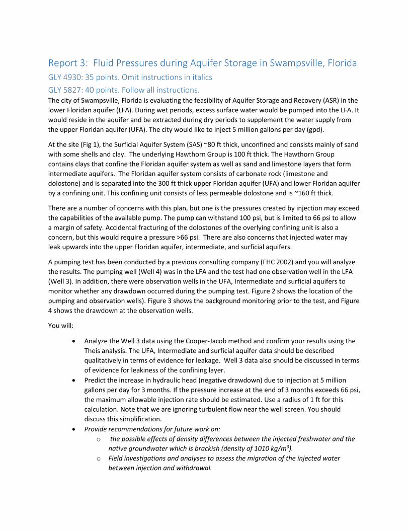
Report 3: Fluid Pressures during Aquifer Storage in Swampsville, Florida

GLY 4930: 35 points. Omit instructions in italics

GLY 5827: 40 points. Follow all instructions. The city of Swampsville, Florida is evaluating the feasibility of Aquifer Storage and Recovery (ASR) in the

lower Floridan aquifer (LFA). During wet periods, excess surface water would be pumped into the LFA. It

would reside in the aquifer and be extracted during dry periods to supplement the water supply from

the upper Floridan aquifer (UFA). The city would like to inject 5 million gallons per day (gpd).

At the site (Fig 1), the Surficial Aquifer System (SAS) ~80 ft thick, unconfined and consists mainly of sand

with some shells and clay. The underlying Hawthorn Group is 100 ft thick. The Hawthorn Group

contains clays that confine the Floridan aquifer system as well as sand and limestone layers that form

intermediate aquifers. The Floridan aquifer system consists of carbonate rock (limestone and

dolostone) and is separated into the 300 ft thick upper Floridan aquifer (UFA) and lower Floridan aquifer

by a confining unit. This confining unit consists of less permeable dolostone and is ~160 ft thick.

There are a number of concerns with this plan, but one is the pressures created by injection may exceed

the capabilities of the available pump. The pump can withstand 100 psi, but is limited to 66 psi to allow

a margin of safety. Accidental fracturing of the dolostones of the overlying confining unit is also a

concern, but this would require a pressure >66 psi. There are also concerns that injected water may

leak upwards into the upper Floridan aquifer, intermediate, and surficial aquifers.

A pumping test has been conducted by a previous consulting company (FHC 2002) and you will analyze

the results. The pumping well (Well 4) was in the LFA and the test had one observation well in the LFA

(Well 3). In addition, there were observation wells in the UFA, Intermediate and surficial aquifers to

monitor whether any drawdown occurred during the pumping test. Figure 2 shows the location of the

pumping and observation wells). Figure 3 shows the background monitoring prior to the test, and Figure

4 shows the drawdown at the observation wells.

You will:

Analyze the Well 3 data using the Cooper-Jacob method and confirm your results using the

Theis analysis. The UFA, Intermediate and surficial aquifer data should be described

qualitatively in terms of evidence for leakage. Well 3 data also should be discussed in terms

of evidence for leakiness of the confining layer.

Predict the increase in hydraulic head (negative drawdown) due to injection at 5 million

gallons per day for 3 months. If the pressure increase at the end of 3 months exceeds 66 psi,

the maximum allowable injection rate should be estimated. Use a radius of 1 ft for this

calculation. Note that we are ignoring turbulent flow near the well screen. You should

discuss this simplification.

Provide recommendations for future work on:

o the possible effects of density differences between the injected freshwater and the

native groundwater which is brackish (density of 1010 kg/m3).

o Field investigations and analyses to assess the migration of the injected water

between injection and withdrawal.

Report format 1) Executive Summary

2) Introduction

a) Objectives

b) Site descriptions

3) Methods

4) Results

a) Pumping test description and analyses

b) Predictions concerning maximum pumping rate

5) Discussion of Results

a) Test problems or concerns

b) Evidence for/against leakage between the LFA and other aquifers

6) Limitations of this study

7) Recommendations for future investigations

8) Conclusions

Appendix 1: Calculations

Report Expectations There are not many calculations for this report, so the analysis should be very well done and clearly

written. Be sure to use the feedback and examples from your previous two reports. The report format

should be followed closely, and the report should address all components of the investigation. The

report should have correct spelling and grammar, and the writing style should be professional. All

figures and tables should be captioned.

In this case, your only source for previous site information is the FHC (2002) report (Full Citation: Florida

Hydrogeology Consultants (2002), Hydrogeology of Swampsville, Florida, 204 pp). Present Figure 1 and 2

as if they came from FHC (2002).

Appendix: Information and Figures (from FHC, 2002)

Well 4 was pumped at a constant rate of 1530 gpm for 48 hours. The drawdown data are linked here.

During the pumping, 1.1 inches of rain fell. This timing will be noted in the data.

Well information for the pumping test

Well Name Description Screen Depth or Open Interval (ft below ground surface)

Horizontal Distance from Pumping Well

Well 4 LFA Pumping Well 680-950 NA

Well 3 LFA Observation Well 680-963 3015

FO-1 UFA Observation Well 181-300 100

HO-1 Intermediate Observation Well

181-300 100

WT-1 Surficial Observation Well

69-79 100

https://drive.google.com/file/d/0B10wizgNjv4CZDZjMGJ5T1Jkc28/view?usp=sharing

Figure 1. Site geology and

hydrogeology (from FHC, 2002).

Figure 2. Site map showing locations of pumping wells, observation wells, and other production wells in

the region. The location of the discharge pipe for the pumping test is also shown.

Figure 3. Background monitoring prior to the pumping test.

Figure 4. Observation well data during the pumping test at Well 4.

Assignment 1: Darcy’s Law and Hydraulic Conductivity 20 points.

Part A: Sediment Description Using the Unified Soil Classification System

Throughout this semester, we’ll use the USCS system to classify sediments. It is very commonly used in

groundwater studies. In this assignment, you’ll examine only one sample. We’ll return to the USCS in

later classes. A chart is provided on the last page.

1. Use a ruler to measure the average size of the grains and provide a sample description. The

sample description should include the grain size distribution (for sand: fine-grained, medium-

grained, coarse-grained, see the table on page 4), whether grains are angular or rounded (or in-

between: subangular or subrounded), the consolidation state of the sample (common terms for

sands/silts are loose and dense, for clays: soft and firm). Often the description will note the clast

type if sands are not primarily quartz.

2. Use the USCS chart to determine the correct two-letter code.

Part B. Hydraulic head and flow direction

Before starting any flow experiments, you'll examine the static case to better understand how elevation

head and pressure head contribute to hydraulic head. For this experiment, we have two reservoirs. One is

on each end of the cylinder of sand. The water levels in the two reservoirs should equal each other, so

there is no flow through the cylinder. If they are not equal, you carefully add/remove water to equalize.

They will eventually equalize through flow, but that takes time.

Two piezometers tap into the cylinder. The cylinder diameter

is 1.25 inches and the distance between the two piezometers

is 13.5 cm.

3. Use a ruler to determine the elevation head, pressure

head, and hydraulic head in the two piezometers (in

cm). Use the wooden base of the stand as your

datum. Assume that the piezometer screen (the

location where it is open to the sediment) is at the

bottom of the tubing where it attaches to the cylinder.

4. Calculate the fluid pressure (in Pa) at each piezometer screen. Assume a fluid density of 1.0

g/cm3.

5. Rotate the cylinder slightly (see figure). The

hydraulic heads in each piezometer should

adjust and return to the same values as

previously because the water levels in the

reservoirs were not changed. What are the new

elevation and pressure heads?

To start flow: Add or very carefully remove water from

the reservoir on the left side of the cylinder to

raise/lower the water level several cm.

6. What are the hydraulic heads in Well A and

Well B and which direction is water flowing?

(Note: It’s not fast, but you should see the water

level rise on one side and drop on the other).

7. Use your understanding of hydraulic head, elevation head, and pressure head to briefly explain

how groundwater can flow "uphill" in the cylinder.

Part C. Measurements and calculations of hydraulic conductivity

At this station, the tubing from the Darcy experiment is

open on one end so that you can measure discharge. The

material in the cylinder is the same as you described (or

will describe) at Station A.

Ensure that you have water in the fluid reservoir on the

left. Place a beaker to catch the outflow. Open the hose

clamps and remove the lid (if on) of the fluid reservoir

to allow flow to begin. Allow the hydraulic heads in the

two wells to stabilize and then measure the hydraulic

head in both of the wells. Use the wooden base as your

datum. Use a beaker or graduated cylinder and a

stopwatch to measure discharge (volume per time).

Conduct two additional runs using different hydraulic

gradients. Try to have one at least one run with a small

(<0.5 cm) head difference.

During Run 2, you will carefully add dye to the tubing

using the syringe. Start timing the dye as it enters the sediments and stop timing as the dye emerges

from the sediments on the downgradient end. If you prefer, you can choose a different distance.

Be sure to run the dye trace using the same hydraulic head difference as your discharge measurement.

If your dye trace during Run 2 doesn’t work out (you forget to start or stop timing, etc), you can try

again during Run 3.

8. (2 pts) Complete the following table of measurements

Run h1 (cm) h2 (cm) Volume

(cm3)

Time (s) Dye

distance

(cm)

Time

for

dye

movement (s)

1

2

3

9. (4 pts) Data from previous experiments using the Darcy cylinder with the same sediment are shown

on the next page. Add your data to the table. For all of the runs, calculate discharge (Q), hydraulic

gradient (i), specific discharge (q), hydraulic conductivity (K), and the Reynold’s number (Re). For

the Reynolds number, use a viscosity of 0.001 kg/(s m) and be careful to convert all other values to

consistent units. Show your work for one of each calculation and use Excel for the remainder. For

Run 2 (or whichever run was your dye trace), you will also calculate velocity and effective porosity.

Notes: you can copy and paste the previous data from the Word version of this handout (online) into

Excel. The calculated results for the data on the first line are provided for you as a check on your

calculations.

10. (3 pts) Using Excel, plot specific discharge as a function of hydraulic gradient and fit a linear

trendline with a zero intercept. Be sure to label your axes and show the equation. Discuss whether or

not the data are well fit by the line. The R2-value should be considered as well as any qualitative

description (e.g., does it fit well at low hydraulic gradients and poorly at higher gradients, is the fit

good except for one or two suspicious values? Do your data plot differently from previous results?).

11. Use the slope of the line to determine the hydraulic conductivity. NOTE: If your results were

drastically different than previous results, please average your results them rather than using the

slope of all measurements. Using Figure 3.2 in your text (copied below), discuss how the measured

K compares to the expected range for its sediment type.

12. Calculate the permeability of the sand (in m2) for the hydraulic conductivity from #11.

13. The threshold for turbulent flow is at a Reynold’s number somewhere between 1 and 10. Do your

Reynold's number calculations suggest that flow is likely to be turbulent during any of the runs?

Explain.

14. Does your plot of specific discharge versus head gradient indicate that the flow during the

experiments was laminar or turbulent? Explain. What would you expect the plot to look like if the

flow becomes turbulent at high specific discharge values?

H1

(cm)

H2

(cm)

Volume

(ml) time (s)

dye

trace

time (s)

dye

trace

distance

(cm)

Q

(cm3/s)

i

(cm/cm)

q

(cm/s)

K

(cm/s)

Re v

(cm/s)

ne

24.6 24.3 9 47 210 15.5 0.19 0.022 0.024 1.1 0.36 0.074 0.33

25.8 25 18 30

25.5 24.8 20 35

25.2 24.4 17 30

27.4 26.8 18 42

25.1 24.7 11.5 44

27 26.7 8 43

Assignment 2: Hydraulic Conductivity 20 points

1. (2 pts) In the previous (Module 1) assignment, you calculated the hydraulic conductivity of

the sand in the Darcy experiment. Return to that assignment to find your estimated K and the

average grain size.

a. Use the Kozeny-Carman equation to calculate the permeability and hydraulic

conductivity of the sand. Use a porosity of 0.33.

b. Discuss how the hydraulic conductivity calculated using the Kozeny-Carman

equation compares to that estimated in the experiment.

Questions 2 to 5 are based on the Cabot/Koppers Superfund in Gainesville, Florida. At this site,

the Hawthorn Group of sediments acts as a confining unit to the upper Floridan aquifer (below)

and separates the upper Floridan aquifer from the contaminated surficial aquifer (above). The

upper Floridan aquifer consists of limestone and dolostone and the surficial aquifer in this region

is primarily sand.

The upper Floridan aquifer is an important water source. The well field for Gainesville Florida is

just a few miles from of the Cabot/Koppers site. Unfortunately, contamination has been found in

the upper Floridan aquifer. This was not expected, because it was assumed that the

contamination would travel very slowly through the Hawthorn Group. To better understand, you

will use calculations to estimate travel times across the Hawthorn Group.

2. (3 pts) The Hawthorn Group of sediments consists of layers of clay, limestone, and clayey

sand. Thicknesses are variable across the site, so ranges are provided below.

From the top down, the Hawthorn Group consists of:

clay 1 to 5 ft thick,

clayey sand 25 to 30 ft thick

limestone: 5 to 10 ft thick

clay 20 to 25 ft thick

clayey sand 40 to 55 ft thick

clay 14 to 30 ft thick

Clay vertical hydraulic conductivity has been measured in the laboratory and is 6.7 x 10-8 cm/s.

The clayey sand vertical hydraulic conductivity is 1 x 10-5 cm/s, and the limestone hydraulic

conductivity is 1 x 10-3 cm/s.

What is the equivalent vertical hydraulic conductivity (in ft/day) in the Hawthorn

Group? Conduct the calculation twice, first using the maximum clay/minimum sand and

limestone thicknesses and second using the minimum clay/maximum sand and limestone

thicknesses.

Hints:

a. Be efficient and add up the total clay, sand, and limestone thicknesses so you can

simplify to three layers (rather than 6).

b. After your first "by hand" calculation, create a formula in Excel. You will be

repeating the calculation below.

c. Be careful about units!

3. (3 pts) To test whether your calculated equivalent vertical hydraulic conductivities are

sensitive to the laboratory-measured value of hydraulic conductivities:

a. increase and decrease the clayey sand hydraulic conductivity by an order of

magnitude. Use the calculation with the thinnest clay/thickest clayey sand and

limestone for this test.

b. increase and decrease the limestone hydraulic conductivity by an order of

magnitude. Use the calculation with the thinnest clay/thickest clayey sand and

limestone for this test.

c. increase and decrease the clay hydraulic conductivity by an order of magnitude. Use

the calculation with the thinnest clay/thickest clayey sand and limestone for this test.

d. Discuss your results and the implications. Which hydraulic conductivity value has the

greatest impact? If you have a limited budget for laboratory testing, which sediment

type would be most important to test? Would you expect the results to be the same for

equivalent horizontal hydraulic conductivity?

4. (3 pts) Hydraulic heads are higher in the surficial aquifer (above the Hawthorn Group) than

in the upper Floridan aquifer (below the Hawthorn Group). The vertical head difference

across the Hawthorn Group is 130 ft and its thickness is 130 ft. Estimated effective porosity

is 0.3. Calculate the following for both your upper- and lower-end estimates of equivalent

vertical K (from #2):

a) vertical specific discharge (in ft/day)

b) vertical velocity (in ft/day)

c) travel time across the Hawthorn Group (in years)

5. (2 pts) The hydraulic conductivity of the upper Floridan aquifer in the area is ~150 ft/day.

Assume the groundwater moves downward almost vertically (an angle of 89°) in the

lowermost clay layer (K=6.7 x 10-8 cm/s). Based on the tangent law of refraction, what would

the angle of flow be in the upper Floridan aquifer?

6. (3 pts) Hydraulic head has been measured at 3 wells shown on the map. All are within the

same aquifer.

Well Top of well elevation (m asl) Depth to water (m) Hydraulic head (m)

1 32.6 5.2

2 33.5 5.5

3 32.4 5.3

a. Calculate the magnitude of the hydraulic gradient. Show the flow direction on the

map, assuming the aquifer is isotropic.

b. Calculate specific discharge (in m/day) for a hydraulic conductivity of 0.24 ft/day.

7. (4 pts) Based on drilling investigations, it has been found that the subsurface at a site consists

of a clay layer (diagonal pattern) overlaying a sand layer.

Piezometer nests were installed, and hydraulic head values are shown on the cross-section below.

a) Contour the cross-section, using a contour interval of 2 ft.

b) Draw three flow lines starting at the three “x” marks. Assume the clay and the sand are

both isotropic.

c) Describe the refraction shown by the equipotentials and the flow lines and explain

whether or not the observed refraction is consistent with your expectations.

d) The hydraulic conductivity of the sand is 30 ft/day. Calculate the specific discharge

through the sand layer between the 32 and 30 ft contours.

Assignment 3: Boring logs and Cross Sections 20 pts

Hydrogeologic cross sections are used to interpret and present the distribution of aquifers and confining

units. Hydraulic heads can also be shown on cross sections to help interpret flow directions.

Part I. Your first cross section will be based on 4 borings. At each of the boring locations, 2 wells – a

shallow well and a deep well, were later installed. The top of each well casing was surveyed to find

elevation in ft above sea level (ft asl) and the depth to water was measured on June 21, 2015.

1. (6 pts) Complete the cross section, following these steps.

Mark the ground surface elevation and connect. In real-life cross sections, you could supplement

this with topographic information from the study area.

Mark the contacts in, measuring down from the ground surface at each well.

Mark the total depth of each boring, but keep in mind that it is not a contact, just the vertical

extend of your information.

Decide how detailed your cross-section needs to be for your purpose. For this cross-section, we

are grouping by “aquifer” material and “confining unit” material and will not mark changes from

silty sand to sand (for example).

Connect similar materials. When sediments are deposited they are often in layers, but not

always. It is possible for a “lens” of sediment to exist either due to how it was deposited or later

erosion.

Label aquifers and confining units. For aquifers, label whether they are confined or unconfined.

Mark in screen locations at each boring (one for the shallow well and one for the deep well. You

may want to color-code the shallow and deep.

Calculate and mark in water-level elevations for each well using an upside-down triangle with a

line underneath. You may want to color-code the shallow and deep.

Create a legend for your cross section showing all symbols used.

Connect water levels to show potentiometric surface, being careful to only connect water levels

screen in the same aquifer.

Draw a flow arrow for the shallow wells and for the deep wells indicating the direction water is

flowing for both.

2. (4 pts) Based on the cross section:

A) Calculate the vertical hydraulic gradient at B-2 as well at B-4. Assume the vertical distance is the

thickness of the confining unit. In other words, assume there are no vertical gradients in the

aquifers.

B) Calculate the horizontal hydraulic gradient between:

a) the shallow wells of B-2 and B-3

b) the deep wells of B-2 and B-3.

Boring and Well Information (Distance relative to the west side of the cross section). Lithologic descriptions given using USCS abbreviations.

B-1 B-2 B-3 B-4

Distance 500 1000 2000 2900

Ground surface elevation (ft asl) 60 60 40 30

Total depth (TD) ft 100 90 80 90

Lithologic Description (ft below ground surface)

0-TD SC

0-40 SC 40-60 ML 60-TD SM

0-40 SC 40-50 CL 50-TD SP

0-20 SC 20-40 CL 40-TD SP

Depth of deep monitoring well screen (ft bgs)

80-90 70-80 50-60 40-50

Depth of shallow monitoring well (ft bgs)

20-30 20-30 10-20 10-20

Elevation of top of well casing for both shallow and deep wells (ft asl)

61 61 41 31

Deep wells (DW) depth to water (ft)

26 29 14 11

DW water level elevation (ft asl)

Shallow wells depth to water (ft)

25 28 10 5

SW WL elev (ft asl)

Part II. Your second cross section will be based on the geology of a Superfund site in the Aberjona River

valley near Woburn, Massachusetts. In this region,

Wells G&H were used for water supply starting in 1964

(Well G) and 1967 (Well H). In 1979, contamination was

found in Wells G & H and both wells were shut down.

During this time, a number of leukemia deaths occurred

in the area supplied by Well G&H.

Subsequent lawsuits attempted to attribute responsibility

for the Well G&H contamination. Understanding the

geology of the Aberjona River valley was an important

part of the investigation. The bedrock of the river valley

has been eroded by glaciation and glacial till was

deposited on the bottom and sides of the valley. After the

last glacial maximum, alluvial sediments filled the valley.

Many borings were drilled and cores were collected.

Your cross section will use the information from drilling

to better understand the aquifer’s geometry and its

heterogeneity.

The cross section location is shown in red on the map.

3. (2 pts) Using the boring logs from Well H and Boring S67 (below), find the land surface elevation and

summarize the lithology similar to the wells shown below.

This is a more challenging cross section than the previous one because there are no distinct

confining units here. You are looking at more subtle differences in material. Therefore you will not be

grouping sediments as “aquifer material” or “confining material” as you did in Part I. Instead, you will

be trying to connect similar geologic material. Use your best judgment (ask for advice where unsure)

as to what sediments should be grouped.

Well H Land Surface

Elevation = Well S67 Land Surface

Elevation =

Depth (feet)

Lithologic Description

Depth (feet)

Lithologic Description

to to

to to

to to

to to

to to

to to

to to

to to

4. (5 pts) Construct the cross-section by drawing in the ground surface and the contacts between

geologic materials.

5. (3 pts) Using the information from the cross section, describe the geometry of the aquifer and how the

hydraulic conductivity would be expected to vary, both laterally and vertically.

Well S65 Land Surface Elevation = 77

Depth Lithologic Top

(feet) Description Elev.

0 to 2 Peat 77

2 to 10 Sand and gravel 75

10 to 27 Silty sand with some cobbles 67

27 to 37 Gravel 50

37 Bedrock 40





10 to 21 Silt (dense) 65

21 to 35 Sand (dense) 54

35 Bedrock 40




0 to 9 Artificial fill 48

9 to 14 Silty sand 39

14 to 60 Sand 34

60 to 69 Silty sand -12

69 to 80 Sand and gravel and silt (dense) -21

80 to 107 Sand and gravel (dense) -32

107 Bedrock -59




0 to 2 Peat 44


42 to 52 Sand 2

52 to 82 Sand and gravel -8




0 to 5 Peat 44

5 to 40 Sandy, organic silt 39

40 to 50 Sand 4

50 to 55 Silty sand -6

Cross-section for Part II:

55 to 100 Sand -11

100 to 105 Sand and gravel and silt -56

105 to 115 Sand -61

115 to 122 Sand and gravel (dense) -71




0 to 15 Sand 47


30 to 35 Sand 17

35 to 66 Sand and gravel with some boulders (dense) 12

66 Bedrock -19

Well H boring log:

S67 boring log (2 pages).

Assignment 4: Florida’s hydrostratigraphy

Natural gamma ray (NGR or “Gamma”) logs are commonly used in Florida to differentiate

lithologic formations within boreholes. Gamma logs are sensitive to vertical changes in

radioactive material with depth.

Phosphate grains within sediments of the Hawthorn Group have a high radioactive signature.

Clay minerals and organic material are moderately radioactive.

Calcite and dolomite generally have low radioactivity

Electric geophysical logs measure differences in electrical potential and the flow of electrical

current through the adjacent formation material. In Florida, resistivity logs are commonly used.

A high porosity rock will be able to conduct an electrical current through the water in the

interconnected pores, and therefore will register a low resistivity. On the other hand, rocks with

low porosity (limited water filled pore-space) will have more resistance to an electrical current

and thus register a high resistivity.

In Florida:

Low porosity evaporite deposits exhibit the highest resistivity values

Low porosity limestones and dolostones show moderate to high resistivities.

High porosity limestones and dolostones typically exhibit low resistivity values.

Fluid salinity will affect electrical response. In the logs you will look at in this assignment,

groundwater is generally fresh and you can assume salinity variations are not a factor.

1. (3 pts) Figures 9 & 10 (linked here) are examples of the relationships between gamma logs,

electric logs, and the geologic formations of Florida. Based on the geophysical logs, discuss

how you would identify the boundary between the following. (Note: In some cases, logs

might not be helpful):

A. The bottom of the Hawthorn Group and the top of the Ocala Limestone?

B. The bottom of the Ocala Limestone and the top of the Avon Park Formation (Fm)?

C. The bottom of the Avon Park Fm and the top of the Oldsmar Fm?

2. (2 pts) A geophysical log from borehole M-0650 is linked here. This borehole is from the the

Silver Springs region in Ocala, FL (~40 miles south of Gainesville).

A. The top of the Avon Park Formation is marked on the geophysical log. As you learned

from the reading, the Avon Park Formation is limestone and dolostone, and part of the

Floridan aquifer system. The cross section shows the Surficial Aquifer System (SAS) but

doesn’t mark in the Hawthorn Group (known as the upper or Intermediate confining

unit). Which log suggests that the Hawthorn Group exists at this site? Explain. Based on

that log, at what depth is the boundary between the Hawthorn Group and the top of the

Floridan aquifer system (Ocala Fm)?

B. The Hawthorn Group is much thinner at this site that at the Cabot-Koppers site in

Gainesville. What must have occurred to “thin” the Hawthorn Group? What must have

occurred to the Suwannee Limestone, which does not appear at this site?

https://drive.google.com/file/d/0B10wizgNjv4Cb1VkbGFFMnNkWEk/view?usp=sharing

https://drive.google.com/file/d/0B918EG_vgUA9eGtOUlZwQS0tcFE/edit?usp=sharing

3. (4 pts) As shown in the cross-section included with the reading, the “Middle Confining Unit”

or “Middle Composite Unit” separates the upper and lower Floridan aquifers. But its

hydraulic conductivity is variable and poorly mapped in northern Florida. Recent

investigations by the St John’s Water Management District (SJWMD) have focused on

drilling this interval at locations where it previously was not mapped.

A. Discuss why the middle confining unit of the Floridan aquifer system is particularly

difficult to characterize (as opposed to the upper confining unit).

B. There is discussion of using more water from the lower portions of the Floridan aquifer

system because the upper portions of the Floridan aquifer are over used. Discuss why it

matters whether or not the middle confining unit exists in north Florida.

C. Explain which borehole geophysical logs might be most helpful in identifying the middle

confining unit and predict how these logs would indicate the presence of a confining unit.

D. Return to the M-0650 log. The middle confining unit is marked with “MCU”. Describe

the gamma, caliper, and electric resistivity (Normal Electric) log responses and discuss

whether they agree with your predictions from “C”.

4. (4 pts) We’ve previously described sediments in class and used lithologic logs from

sediments. Lithologic logs in carbonate aquifers rely on a lot of specialized information. The

linked Excel spreadsheet from the SRWMD provides a view of the detailed information

collected from core descriptions. These are from a boring M-0738, which is located in

Marion County near M-0650.

A. Sheet M-0738_Litho_Unit_Picks has a table with the depths chosen for the contacts

between geologic formations. Make note of the depth for the top of the Avon Park Fm

(which is the boundary between the Ocala Limestone and the Avon Park Fm), then

switch to the lithologic description sheet and find that depth. Answer the following

questions based on the columns of main properties (primary rock type, primary porosity,

limestone grain type, dolomite alteration, induration, cement type, and index fossils),

looking immediately above and below the top depth marked for the Avon Park Fm.

-What properties change across this contact?

-What properties remain the same across this contact?

B. Examine the primary rock types and their respective primary porosities. Is there any

obvious relationship between primary rock type (limestone vs dolostone) and porosity

type?

5. (2 pts) Inspect the geophysical logs for M-0738. (linked here)

A. There are multiple spikes in the natural gamma log within the FAS. Similar spikes were

observed at M-0650. Predict what could cause high gamma values in a carbonate

sequence?

B. Examine the lithologic log descriptions for the depths of the gamma spikes at M-0738.

Does the lithologic information support your prediction?

https://drive.google.com/open?id=0B918EG_vgUA9ZHNUak9yWkdUWkE

https://drive.google.com/file/d/0B918EG_vgUA9S1dlSkRLR3JJSnc/view?usp=sharing

6. (2 pts) The middle confining unit was observed at a depth of 190 ft at M-0650. Does the

character of the resistivity spike from M-0650 better match the M-0738 spike at 160 or the

spike at ~200 ft? Explain.

7. (2 pts) Examine the core descriptions on the Excel spreadsheet for M-0738 for either 160 ft

or ~200 ft (whichever your pick was for the confining unit). Do the lithologic descriptions

support the interpretation that this interval acts as confining unit relative to the overlying

rock? Explain.

8. (1 pt) Suggest two distinct tests or data collection that could be used to determine whether

this interval tentatively identified as a confining unit is lower permeability than the overlying

and underlying rock.

Assignment 5 Groundwater Storage and Flow Equations

Part I

The first six questions examine storage in the northern portion of the Gulf Coast aquifer system. This

coastal plain aquifer consists of sands and clays, ranging from unconsolidated near the surface to semi-

consolidated at depth. The aquifer system has an area of ~68,000 square kilometers, and groundwater is

under semi-confined to confined conditions. The aquifer is ~2000 feet thick. Between 1970 and 1980, the

average reduction in storage was 0.6 million acre-feet per year. An average hydraulic head drop of 10 feet

and an average subsidence of 0.5 feet were observed over the aquifer area. Note: This might not sound

like much subsidence, but keep in mind that the subsidence will be much greater than average in the

active pumping areas.

For the calculations, assume a porosity of 0.05, a fluid density of 1000 kg/m3 and a fluid compressibility

of 4.4 x 10-10 Pa-1.

1 acre-foot=1234 m3

1 m= 3.2808 ft

1. Calculate the volume of water (in m3) removed from storage in the 1970s.

2. Use the volume of water removed, the aquifer area, and the hydraulic head change to calculate the

apparent storativity (unitless) of the aquifer system. Use Eq 6.29.

3. Hydrogeologic studies that examined seasonal changes in hydraulic head due to changes in

pumping and recharge found storativity values averaging 0.001. Why is it reasonable that this

value is less than the storativity estimated from the decade-long hydraulic head change?

4. Calculate the specific storage of the aquifer system (in 1/m) based on the storativity and the

aquifer thickness.

5. Calculate the matrix compressibility of the aquifer system (in 1/Pa) using Equation 6.27 in your

text.

6. Equation 6.27 is only valid if n. Calculate n to confirm

Part II

The following three questions refer to the High Plains aquifer. In parts of Texas, the High Plains aquifer

saturated thickness has decreased from 100 feet to 50 feet due to pumping. The aquifer is unconfined and

the specific yield is estimated to be 0.15. Estimated specific storage is 1 x 10-7 1/ft.

7. Your text states that for an unconfined aquifer, S=Sy, or storativity equals specific yield. Yet,

elastic storage due to compression still occurs in unconfined aquifers. More accurately, S=Sy + Ss

x b (where b is aquifer thickness). Use this equation to calculate the storativity of the High Plains

aquifer.

8. How much has the volume of water stored in the aquifer decreased (in ft3 per square foot of

aquifer area)?

9. If hydraulic conductivity is 50 ft/day, how much would transmissivity decrease (in m2/min) as

the saturated thickness decreased from 100 to 50 feet?

Part III (11 pts) consists of a simplified approach to the groundwater flow equations. This will be worked

through in class, and graded on a completion basis.

Assignment 6: Potentiometric Surface Maps

Please complete contours and calculations on paper and submit in class next Weds.

Objectives:

Learn to draw and interpret potentiometric surface maps.

Practice calculations of equivalent horizontal and vertical hydraulic conductivity

Evaluate whether several industrial sites could have contributed to contamination at

water-supply wells by drawing flow lines and calculating travel times.

Part I: Warm-up map. It’s a really good idea to have us look over your map and calculations

before you start on Part II.

1. The map below shows hydraulic head data (in ft) from an unconfined isotropic aquifer

and a stream (shown as a solid line) that is hydraulically connected to the aquifer.

A. (2 pts) Contour the data using a 10 foot contour interval. Label your contours and be

sure to use the stream levels in addition to the monitoring well hydraulic heads.

B. (1 pt) Draw in the groundwater divide on your contour map as a dashed line.

C. (1 pt) Draw 3 flow lines starting at the star, and at each of the 2 “happy faces”.

D. (1 pt) Calculate the hydraulic gradient between the “star” and the stream.

Note: You do not need to estimate the hydraulic head at the star and the stream. You

can calculate hydraulic gradient between two contours.

E. (1 pts) Assuming K=15 ft/day and ne=0.12, calculate the travel time between the

“star” and the stream.

Part II

The attached map shows hydraulic heads (in feet above mean sea level, or asl) from 2008 for the

upper Floridan aquifer (UFA) in the Gainesville, FL area. Two versions are provided because the

hydraulic head values are easier to read and contour without the background map. It is suggested

that you first contour the version without the background map and then transfer your contours.

In the map area, the upper Floridan aquifer transitions from unconfined in the south and west to

confined conditions in the north and east. Gainesville’s water is pumped from the upper Floridan

aquifer, just north of 53rd Ave (~ where you see the 27.74 ft asl water level).

1. (5 pts) Sketch a potentiometric surface map for the upper Floridan aquifer. Use a 5 foot

contour interval. Draw the 10 foot intervals (80,70,60 ft, etc) first, and then fill in the “5”s.

Label your contours.

2. (1 pt) The Cabot-Koppers hazardous waste sites are located in Gainesville approximately

where the 43.82 ft reading is located. Assume that the aquifer is isotropic, and draw a

flowline from this location. Does the groundwater from this site flow to the well field’s cone

of depression?

3. (4 pt) Find and justify reasonable values for the hydraulic conductivity and effective porosity

of the upper Floridan aquifer. Use these values to calculate travel time (in years) from the

Cabot-Koppers site to the Gainesville well field. Because the hydraulic gradient changes

drastically as you approach the cone of depression, break the calculation into two segments.

First calculate the hydraulic gradient and travel time for the segment from the location of the

well with a hydraulic head of 43.82 ft to the 40 ft contour. Next calculate the hydraulic

gradient and travel time from the 40 ft contour to the well with a hydraulic head of 27.74 ft.

Add the two travel times to find the total.

Other features to observe on the potentiometric surface map:

4. (1 pts) Use a dashed line to sketch the location of the groundwater divide south (to southeast)

of Gainesville. There is a ridge that separates groundwater that flows roughly north (and to

the well field from groundwater that flows south to Payne’s Prairie.

5. (1 pt) What is the relationship between the equipotential lines and surface water north and

east of Gainesville? For example, look at the Santa Fe River near Hampton Lake to see if

there are any indications that it is gaining or losing water. Explain – why does this make

sense for an area where the aquifer is confined?

6. (1 pt) Examine the relationship between the equipotential lines and the Santa Fe River on the

west side of your map (near Fort White). Is the Santa Fe River gaining or losing water from

the UFA at this location?

Scale: 1:635000

Assignment 7 Recharge and the Hydrologic Cycle

In this assignment, you’ll examine recharge estimates and groundwater ages at two locations: 1)

Great Artesian Basin in Australia; and 2) Silver Springs group springshed near Ocala Florida.

Part I: Great Artesian Basin in Australia

The Great Artesian Basin is a structural basin, which means that it is lower in the center than at

the sides. The aquifers in the basin are sandstones and the confining units are mostly shales.

There are some similarities to the Dakota Sandstone aquifer (Figure 5.3.9 in your text). Both

aquifer systems consist of more than one sandstone layer that is recharged where exposed, and

confined by shales elsewhere. There is also a shallower unconfined aquifer above the sandstone.

Differences are that recharge of the Dakota sandstone generally occurs on the western side only

(with discharge on the eastern side). Another view of the GAB can be found at this link. Data

and the potentiometric surface map are from Bethke et al (1999).

1. Groundwater in the confined Great Artesian Basin in Australia has been dated and ages up to 2

million years have been determined. What radioactive tracer could have been used for these

ages?

http://wetlandinfo.ehp.qld.gov.au/wetlands/ecology/aquatic-ecosystems-natural/groundwater-dependent/sedimentary-rocks-great-artesian-basin/sedimentary-basins.html#modhydrology

http://onlinelibrary.wiley.com/doi/10.1029/1999JB900085/pdf

2. To the right, ages are plotted at

various distances from the

northeastern recharge area (see the

map for the location). You’ll

notice that the error bars get larger

for the older ages. Use the ages

and distances to calculate average

velocity (in m/year).

3. The long-term average recharge rate will be the same as specific discharge. If the effective

porosity of the sandstone in the Great Artesian Basin is 0.23, what is the long-term average

recharge rate in m/year and in m/day?

4. (4 pts) Next you will use Darcy's law, estimated hydraulic conductivity and effective

porosity, and the potentiometric surface map (contours are in m) to calculate a second

estimate of recharge rate.

a. Calculate hydraulic gradient between the 500 and 100 m contours along the cross-

section line. Note that this is not an exact flowline, but sufficient for this rough

calculation.

b. Average hydraulic conductivity is 2.0 m/day. Estimate the specific discharge (in

m/day).

c. Effective porosity is 0.23. Calculate velocity.

d. Briefly discuss how the velocity result compares to the velocity estimated from the

age estimates (Question 2). One explanation for the difference is the faults observed

in the cross section. How might faults reduce horizontal hydraulic conductivity in the

sandstone layers?

5. (3 pts) In the western recharge area for the Great Artesian Basin aquifer, two boreholes (DR-

3 and DR-4) were drilled in the unsaturated zone. The pressure (tension) was measured, and

can be converted to pressure head by multiplying by water density of 1000 kg/m3 and

gravitational acceleration). You'll notice that: 1) the unsaturated zone is quite thick (80 m)

and 2) the pressure heads are very low (extremely negative). As a result of the extremely low

pressure heads, changes in elevation are small compared to changes in pressure head.

Inferred flow directions (upward or downward) are shown with arrows.

a. What do the flow directions

indicated by the pressure heads

suggest about groundwater

recharge at the present time?

b. Carbon-14 dating of recharge

indicates ages up to 30,000 years at

the water table. What does this

suggest about recharge? Is that

conclusion consistent with the results

from the studies of the unsaturated

zone? Is it consistent with the

conclusions from age dating within

the aquifer?

c. Why might the long-term average (100,000s of years) indicated by the age dating be

significantly greater than the current recharge?

Part II: Silver Springs Group springshed near Ocala Florida

The Silver Springs group discharges groundwater from the upper Floridan aquifer to begin the

Silver River. You examined cores and geophysical data from this region in Module 4. The

figure below is from Phelps (2004) and shows the location as well as the potentiometric surface.

The groundwater basin (or springshed) has an area of 2 x 1010 ft2. In the 1960s, pumping was

minimal in the springshed and the discharge from the springs averaged 820 cubic feet per second

(cfs). The basin has no other groundwater or surface water inflows/outflow. Due to the aquifer's

high permeability, runoff is negligible.

1. Recharge calculation

(2 pts)

A) Use a steady-state

water budget to

calculate the

aquifer’s recharge

in ft3/day.

B) Calculate the

recharge rate (per

unit area) in

inches/year.

2.The average rainfall in

the Ocala Florida region is

53 in/year. Using the

recharge rate calculated in

the previous problem,

calculate the percentage of

rainfall lost to ET.

2. (5 pts).

Calculating

http://pubs.usgs.gov/sir/2004/5144/pdf/sir20045144.pdf

groundwater ages from the potentiometric surface map.

a. Using the potentiometric surface map, calculate the average hydraulic gradient (in

ft/mile) from the 80 ft contour near the northern end of the springshed to the 45

foot contour marking the spring group.

b. Transmissivity of the upper Floridan aquifer is extremely variable, but estimates

for the region are 2 x 106 ft2/day. Recall from Assignment 4 that the top of the

middle confining unit is at ~190 to 200 ft below land surface. Assume that the

water table is approximately at the land surface and calculate hydraulic

conductivity (ft/day) from the transmissivity.

c. Calculate specific discharge (in ft/day) based on the hydraulic conductivity and

hydraulic gradient.

d. Effective porosity is estimated to be 0.20. Calculate the velocity (in ft/day).

e. Calculate the travel time (in years) from the 80 ft contour to the 45 ft contour.

f. Based on your predicted age, what tracers would be best used to determine age?

3. (2 pts) Because the UFA is unconfined in much of the springshed, recharge of young

water can occur throughout the basin. Because the unsaturated zone is very thin, this

recharge is expected to be rapid (days). It is also possible that water from the lower

Floridan aquifer could contribute to the discharge at the Silver Springs group. How

would each of these factors impact the inferred ages (based on tracer analyses) of Silver

Springs water?

Assignment 8 Flow to Wells (20 pts)

Each part has two questions. For the first of each type, the answer will be linked from the online

discussion. Check your answer with the solution example. Work through the second on your

own. Because the answers are given on the odd questions (first of each type) you must show

your work on all questions.

Part I. Thiem Solution

1. (2 pts) A well in a 20 m thick confined aquifer was pumped at 100 m3/day until it reached

steady state conditions, and hydraulic heads were measured at two observation wells. The

drawdown at a well located 10 m from the pumping well was 2 m and the drawdown at a

well located 100 m from the pumping well was 1 m. Use the Thiem solution to calculate

the transmissivity (T) in m2/day and K in m/day.

2. (3 pts) A well in a 100 m thick confined aquifer was pumped at 700 m3/day until it

reached steady state conditions, and hydraulic heads were measured at two observation

wells. The drawdown at a well located 5 m from the pumping well was 2.5 m and the

drawdown at a well located 50 m from the pumping well was 0.75 m. Use the Thiem

solution to calculate the transmissivity (T) in m2/day and the hydraulic conductivity (K)

in m/day.

Part II. Theis Forward Solutions

3. (2 pts) For a transmissivity, T, of 2500 m2/day, storativity, S, of 0.00015, and pumping

rate, Q, of 950 m3/day, calculate drawdown in a confined aquifer for r =75 m at t=450

min using the Theis solution. Use the table in the reading to find W(u).

4. (3 pts) For a transmissivity of 1000 m2/day, storativity, S, of 0.0010, and pumping rate,

Q, of 1000 m3/day, calculate drawdown in a confined aquifer for r =20 m at t=300 min

using the Theis solution. Use the table in the reading to find W(u).

Part III. Theis Inverse Solution

The linked spreadsheet should be used for the Theis inverse solution. Download the spreadsheet

and open in Excel. To use the spreadsheet:

a. Make sure your units are consistent.

b. Enter the pumping rate and radius on the spreadsheet.

c. Copy and paste the observation data into the spreadsheet.

d. By trial and error, adjust transmissivity and storativity until the Theis curve

matches the data as best as possible. Decreasing the transmissivity will shift the

Theis curve up (and slightly over). Increasing the storativity will shift the Theis

curve to the right.

5. (2 pts) The linked time-drawdown data are from a test where a well was pumped at a rate

of 5760. ft3/ day. Drawdown was measured in an observation well 300 ft away from the

pumped well. Assume that the pumping and observation well were both screened over the

entire thickness of the confined aquifer. The geologist's log of the pumping well is in ft

below ground surface (bgs):

0 - 23 ft bgs Silty sand

23 - 77 ft bgs Clay

77 - 82 ft bgs Poorly sorted gravel

82 - 117 ft bgs Unfractured granite

Find the transmissivity, storativity, hydraulic conductivity, and specific storage of the

aquifer. You don’t need to submit the spreadsheet. Show your transmissivity and storativity

values below and show calculations for K and Ss.

6. Values of drawdown and time from a constant-rate pumping test are linked here. Both the

pumped well and the observation well screen the entire aquifer thickness, and the

observation well is 35 ft from the pumping well. A pumping rate of 100 ft3/day was used

for the test.

https://drive.google.com/file/d/0B10wizgNjv4CYk5fSDZyZU1ZcGM/view?usp=sharing

https://drive.google.com/file/d/0B10wizgNjv4Cd1Q1WVlwYVhrd00/view?usp=sharing

https://drive.google.com/file/d/0B10wizgNjv4CNm9MZHh0VE5KMkU/view?usp=sharing

The geologist's log of the pumping well is

0 - 120 ft bgs Clay

120-160 ft bgs Limestone, high porosity, some dissolution

160-200 ft bgs Shale

Determine the transmissivity, storativity, hydraulic conductivity and specific storage of

the aquifer.

Part IV. Cooper-Jacob Solution

7. (2 pts) A well in a confined aquifer was pumped at a rate of 7.5 ft3/min. Time-drawdown

data from an observation well located 80 feet away are plotted on a semi-log plot. Use the

Cooper-Jacob method to calculate the transmissivity (in ft2/min) and storativity of the

aquifer. Show your line, your location where you measure Δs and your to location, as

well as calculations.

8. (3 pts) Values of drawdown and time from a constant-rate pumping test are plotted. Both

the pumped well and the observation well are fully penetrating, and the observation well

is 150 m from the pumping well. A pumping rate of 10,000 m3/day was used in the test.

Determine the transmissivity (in m2/day) and storativity of the aquifer using the Cooper

Jacob solution. Show your line, your location where you measure Δs and your to location,

as well as calculations.

Assignment 9: A spreadsheet groundwater model (20 pts)

In this assignment, you will work with an Excel spreadsheet that is a very simplified steady-state model

of an aquifer. The model will be used to predict the maximum rate at which a new pumping well can

extract water without causing stream water to enter the aquifer. Prior to using the model for prediction,

you'll calibrate the model using data from observation wells.

Study Area

The 50 ft thick unconfined aquifer consists of mostly sand with some thin clay layers, and receives 20

inches a year of recharge (per unit area). Slug tests and pumping tests have been conducted and found that the

hydraulic conductivity is between 1 and 20 ft/day.

For the modeling, it is assumed that the aquifer is at a steady-state over the long term and that it is

homogeneous and isotropic.

The stream is on the north end of the aquifer and has a

water level of 110 ft above sea level on the west side

and 101 feet on the east side.

There is a groundwater divide to the south (so no flow

crosses the boundary). The east and west boundaries

also have no flow, and represent the physical limits of

the aquifer. The aquifer dimensions are 900 ft (N-S)

x 1800 ft (W-E).

The location of the proposed new pumping well is

shown on the map.

The Spreadsheet Model

The spreadsheet model discretizes the aquifer (breaks the aquifer into grid cells) and solves for hydraulic

head in the center of every cell simultaneously. Each Excel cell represents a 50 ft x 50 ft area of the

aquifer.

Because the hydraulic head in each cell is affected by the neighboring cells, the model will need to

“iterate”, or repeatedly calculate hydraulic head at every one of the cells until the hydraulic heads satisfy

both Darcy's law and conservation of volume (the amount coming into each cell has to equal the amount

going out).

Download and open the Excel file. When you first open the excel spreadsheet, it might give you a

warning about a circular reference. That is expected, because the solution requires iteration (as described

above). To enable iterations in Excel 2013 for PC: Go to the File pulldown menu and choose options,

then Formulas. Click on the

checkbox to Enable Iterative

Calculations, Change the

maximum number of iterations to

5000 and maximum change to

0.0001 then say OK. If you are

using a different version of

Excel, you can use the Excel help

menu and search for “iterations”.

https://drive.google.com/file/d/0B10wizgNjv4CUTJtQlJjSTBMOW8/view?usp=sharing

Calibrating the Model

Before you can use the model for prediction, the hydraulic conductivity must be calibrated by

comparison to observations. Right now, the model is calculating the hydraulic heads for a hydraulic

conductivity of 1 ft/day. The pumping well rate is zero ft3/day because the well has not yet started

pumping.

There are five observation wells where water levels have been measured over several years and you will

use the average values to calibrate the steady-state model. The measured hydraulic head values are

shown in the spreadsheet just to the right of the shaded region. The spreadsheet also shows the simulated

values. If the model is well calibrated, the simulated values should match the observed values.

1. Enter the known recharge rate of

20 inches/yr (if it is not already

entered). Compare the simulated

and observed hydraulic heads.

Are the simulated hydraulic heads

too high or too low?

2. Our simulated hydraulic gradient is too high, causing the hydraulic heads to be too high. To lower

the observed hydraulic heads in the aquifer, should we increase or decrease the hydraulic

conductivity in the model? Explain your answer using Darcy's Law.

3. Change the hydraulic conductivity to

20 ft/day by replacing the "1" by a "20"

and hit enter. What happens to the

hydraulic head values in the aquifer?

Does this agree with your

expectations?

4. (3 pts) Vary hydraulic conductivity between 1 and 20 ft/day to find the K (to the nearest ft/day) that

provides the best match between the simulated and observed hydraulic heads. If you are strategic,

you do not have to try every possible K value.

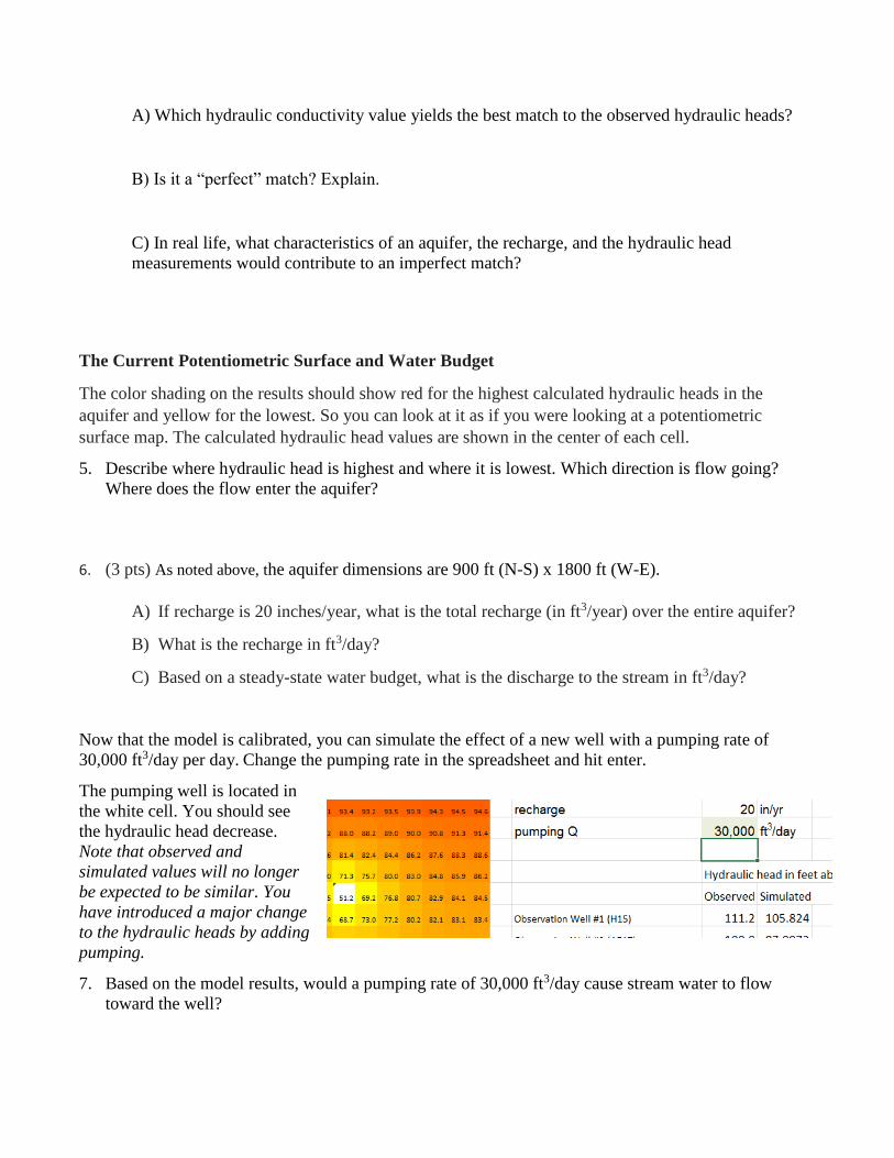
A) Which hydraulic conductivity value yields the best match to the observed hydraulic heads?

B) Is it a “perfect” match? Explain.

C) In real life, what characteristics of an aquifer, the recharge, and the hydraulic head

measurements would contribute to an imperfect match?

The Current Potentiometric Surface and Water Budget

The color shading on the results should show red for the highest calculated hydraulic heads in the

aquifer and yellow for the lowest. So you can look at it as if you were looking at a potentiometric

surface map. The calculated hydraulic head values are shown in the center of each cell.

5. Describe where hydraulic head is highest and where it is lowest. Which direction is flow going?

Where does the flow enter the aquifer?

6. (3 pts) As noted above, the aquifer dimensions are 900 ft (N-S) x 1800 ft (W-E).

A) If recharge is 20 inches/year, what is the total recharge (in ft3/year) over the entire aquifer?

B) What is the recharge in ft3/day?

C) Based on a steady-state water budget, what is the discharge to the stream in ft3/day?

Now that the model is calibrated, you can simulate the effect of a new well with a pumping rate of

30,000 ft3/day per day. Change the pumping rate in the spreadsheet and hit enter.

The pumping well is located in

the white cell. You should see

the hydraulic head decrease.

Note that observed and

simulated values will no longer

be expected to be similar. You

have introduced a major change

to the hydraulic heads by adding

pumping.

7. Based on the model results, would a pumping rate of 30,000 ft3/day cause stream water to flow

toward the well?

8. (4 pts) Drawdown and budget changes:

A) How much drawdown occurs at the pumping well? (You might have to change the pumping rate

back to zero to determine the hydraulic head before pumping).

B) Given that the aquifer thickness is 50 feet, why might that amount of drawdown be unrealistic?

(What would happen to your pump?)

C) Even if this much drawdown were possible, what negative impacts could this much drawdown

have on the aquifer?

D) Look back at your steady-state water budget for the aquifer. Is a pumping rate of 30,000 ft3/day

possible without pulling stream water into the aquifer or removing water from groundwater

storage?

9. Use trial and error to find the highest pumping rate (to the nearest 1,000 cubic feet per day) that can

be pumped without water flowing from the stream to the well. There should be a “groundwater

divide” in between the stream and the well. On the north side of the divide, groundwater flows to the

stream. South of the divide, groundwater flows to the well.

Highest pumping rate: _______________

10. Write a new quantitative groundwater budget for the aquifer with pumping at the rate that you

determined. To balance the budget, what budget term must change?

11. This simulation was for steady-state conditions (e.g., long-term averages of recharge and pre-

pumping hydraulic heads). In real life, streams have water levels that vary through time and recharge

changes through time. How might those changes affect your conclusions?

12. What additional data or parameters would be needed for a transient simulation? (Hint: What

information is needed to solve any transient groundwater flow problem that is not needed for steady-

state groundwater flow problems?)

13. The model can help you get a general feel for the relationship between hydraulic conductivity and

the shape of the cone of depression. For your optimal pumping rate, increase and decrease the

hydraulic conductivity and describe how the cone of depression is affected. Does this result agree

with your expectations based on Module 8?

Assignment 10: Contaminant Transport

In this assignment, you'll return to the Woburn Well G&H Superfund site where contamination was

found in the water supply for Woburn Massachusetts. Following leukemia deaths and discovery of some

abandoned drums, investigations attempted to determine the source(s) of the contamination.

The first part of the assignment focuses on creating contour maps showing the distribution of dissolved

TCE in the Aberjona River Valley area. The second part of the assignment uses an Excel spreadsheet to

calculate the rate of transport of dissolved TCE in the Aberjona River Valley aquifer. TCE refers to

trichloroethylene, which is a man-made solvent. It often acts as a DNAPL. Although there are likely

TCE DNAPLs in the Aberjona River valley, the assignment will focus only on migration of dissolved

TCE.

Maps of concentrations from 3 different time periods are included below. The dimensions on the side

are distance in feet.

1. (1 pt) Carefully review the potentiometric surface during pumping of Wells G & H shown on the

next page. Discuss the flow patterns relative to the pumping Wells G & H, the Aberjona River,

the Riley Well, and the three potential source sites (A, B, and C). A larger version of the map is

linked here).

2. (1 pt) Wells G&H were only pumped during the summer months. How would variation of the

potentiometric surface through time be expected to affect the migration of the contaminant

plumes?

3. (1 pts) In Assignment 3 you constructed a geologic cross-section through the Aberjona River

Valley near Wells G&H. Refer back to your completed cross-section. Discuss how you’d expect

the geology of the site to influence contaminant transport. Keep in mind the role of

heterogeneity in mechanical dispersion.

4. (4 pts) For each of the three maps, contour the concentrations for 10 micrograms per liter (g/L),

50 g/L, 100 g/L and depending on which map is being used, possibly 500 g/L and 1000

g/L. When contouring, start with the highest concentrations and work downward. If you are not

certain whether or not to connect two regions with high concentrations, consider groundwater

flow directions.

Many of the monitoring wells were not drilled until after 1984. The absence of monitoring well

data (labeled as an NA on the 1979 through 1984 map) should be considered when interpreting

the distribution of TCE and answering the questions below.

5. (4 pts) Using the contour maps, answer the following questions.

A. Describe the locations of the highest concentrations and the distribution of TCE for each map.

B. In early investigations and the legal trial, 3 potential groundwater sources were identified

(marked A, B, and C on the map). Based on the concentration contours, do you agree that

these are probable contamination sources? Are there other likely sources?

C. Can you make any conclusions as to which of the three potential sources identified (A, B, and

C) is most likely responsible for the contamination of Wells G&H? Can any of the three potential

sources be ruled out as not at fault for contamination of Wells G&H? Explain your reasoning.

D. If it were possible to go into the past and sample more wells, where would additional samples

be most helpful? Mark the locations on the 1985-89 map and explain your reasoning.

http://ce547.groups.et.byu.net/woburn/usgs/plates/usgs_plate_5.tif

Part II.

This second part of the assignment demonstrates how advection, diffusion, and dispersion influence the

travel velocity and concentration of a TCE plume at Woburn, Massachusetts. It is an analytical solution

worksheet in EXCEL format for one-dimensional advective transport with dispersion considered. The

Ogata-Banks solution (Ogata and Banks, 1961; see page 557 in your text) is embedded into the linked

Excel spreadsheet to calculate concentration at a specific time.

The worksheet calculates the movement of the dissolved TCE plume at 800, 1000, and 1200 feet and

assumes no retardation of TCE movement (related to absorption or degradation) within the aquifer.

Download the spreadsheet.

When the data are entered, the table below the input parameters will populate showing time intervals

(column t), the calculated ratio for the concentration at time t per initial concentration (C/C0) at a defined

distance from the source, the concentration for a specific time t (C) at a defined distance from the

source. The complementary error function is part of the calculation of the analytical solution, and is also

shown. The table is repeated in three sets of columns with each set of columns representing the distances

of 800 feet, 1000 feet and 1200 feet from the source. This type of calculation is valuable in estimating

the time of arrival of a contamination plume from a given source. The accuracy of this time is dependent

on the homogeneity of the aquifer media and how well the velocity and mechanical dispersion are

known.

Hydrogeologic data from the unconfined aquifer underlying the Aberjona River valley at Woburn

indicate that the aquifer has a hydraulic conductivity of 400 ft/d, an effective porosity of 30% (Metheny,

2004), and an average hydraulic gradient of 0.001 (Myette et al., 1982). The longitudinal dispersivity is

assumed to be 25 ft. and the coefficient of molecular diffusion is assumed to be 1x10-6 ft2/day. For

initial concentration, use the highest concentration measured during the sampling.

6. (2 pt) According to drinking water standards, the maximum contaminant level (MCL) for TCE is 5

g/l. How many days would it take before the MCL was exceeded at the 800 feet location, the 1000

feet location, and the 1200 feet location?

7. (2 pts) How would you expect longitudinal dispersivity, the coefficient of molecular diffusion,

hydraulic conductivity, effective porosity, and hydraulic gradient to affect the shape of the

concentration-time curve arrival times?

8. (2 pts) Test the effects of each, by entering different parameter values and viewing the plot. Do

results agree with your expectations?

9. (2 pts) Return to the original parameters and change the distance of “x3” from 1200 ft to the

horizontal distance from Source Site “A” to Well H. The scales on the sides and bottom of the maps

are in feet. How long it would take concentrations near Well H to exceed the MCL after

contamination was introduced at Source Site “A”?

10. (1 pts) The actual transport is 3-dimensional. Discuss how the concentration-time plots would be

affected by 3D dispersion and diffusion.

https://drive.google.com/file/d/0B10wizgNjv4CM3RfcGwwbjNwM1U/view?usp=sharing

https://drive.google.com/file/d/0B10wizgNjv4CM3RfcGwwbjNwM1U/view?usp=sharing

UCC: External Consultations

Rev. 10/10

External Consultation Results (departments with potential overlap or interest in proposed course, if any)

Department Name and Title

E-mailPhone Number

Comments


E-mailPhone Number

Comments


E-mailPhone Number

Comments