Embed Size (px)
Citation preview
1
Construction Management, 3/E by Daniel W. HalpinCopyright © 2006 by John Wiley & Sons, Inc. All rights reserved.
Scheduling – PERT Networks and Linear Operations
ByDr. Ibrahim Assakkaf
Construction Management, 3/E by Daniel W. HalpinCopyright © 2006 by John Wiley & Sons, Inc. All rights reserved.
VRML Applications in Construction
• The Need– Traditionally, construction process information is
communicated with paper document and 2D CAD drawings,
– Recently, the industry has embraced many kinds of web-based technologies, but construction still uses document-based models.
– It is believed that transition to model-based information can be done through web-based 3D user interfaces.
2
Construction Management, 3/E by Daniel W. HalpinCopyright © 2006 by John Wiley & Sons, Inc. All rights reserved.
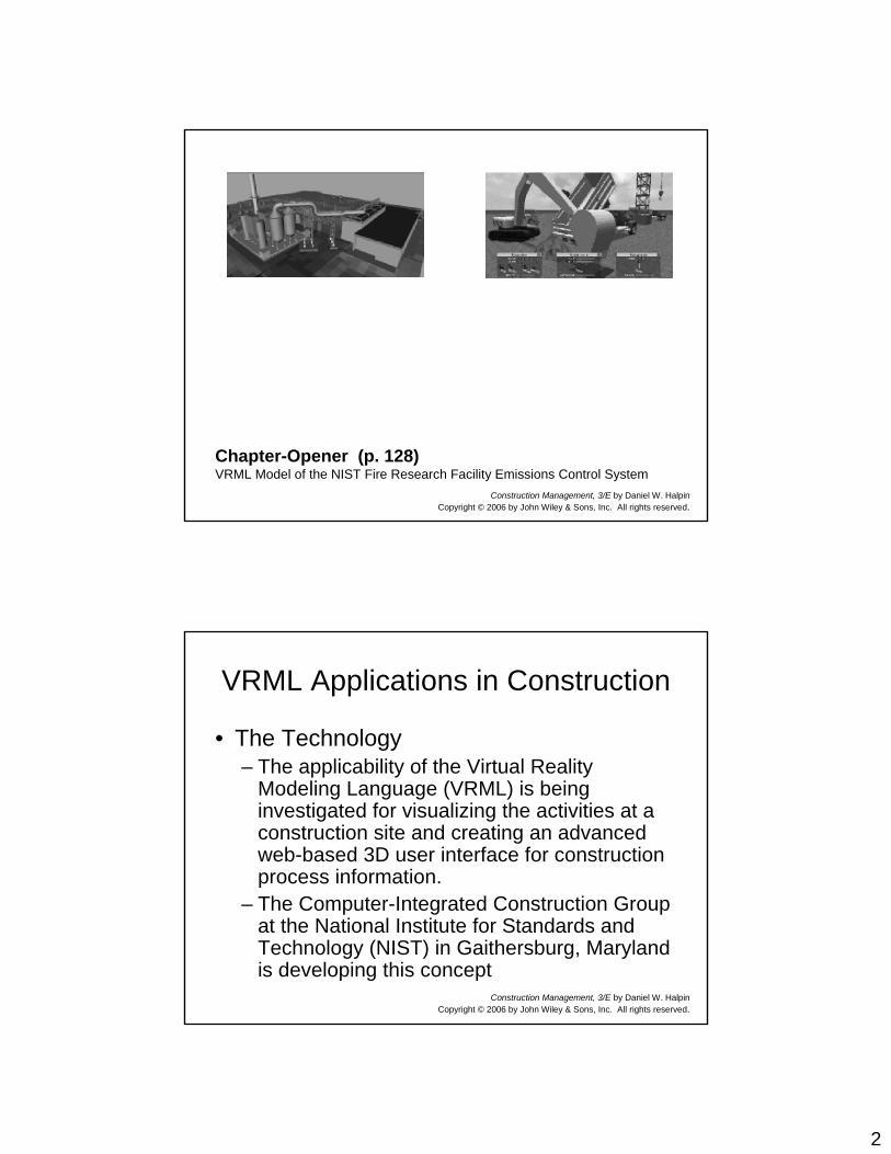
Chapter-Opener (p. 128)VRML Model of the NIST Fire Research Facility Emissions Control System
Construction Management, 3/E by Daniel W. HalpinCopyright © 2006 by John Wiley & Sons, Inc. All rights reserved.
VRML Applications in Construction
• The Technology– The applicability of the Virtual Reality
Modeling Language (VRML) is being investigated for visualizing the activities at a construction site and creating an advanced web-based 3D user interface for construction process information.
– The Computer-Integrated Construction Group at the National Institute for Standards and Technology (NIST) in Gaithersburg, Maryland is developing this concept
3
Construction Management, 3/E by Daniel W. HalpinCopyright © 2006 by John Wiley & Sons, Inc. All rights reserved.
VRML Applications in Construction• The Technology (cont’d)
– In principle, VRML is an open standard that offers the possibility of accessing many types of construction project data readily available and well-accepted graphical user interfaces.
– These interfaces are based on web-based 3D visualizations of a model.
– In order to view the VRML world, the users should have a VRML browser, which can be stand-alone application, a helper application, and/or a plug-in.
– Using this environment, models such as these pictures on the next slide can be readily developed.
Construction Management, 3/E by Daniel W. HalpinCopyright © 2006 by John Wiley & Sons, Inc. All rights reserved.
Introduction
• Bar charts and critical path method )CPM) network assume that all activity durations are constant or deterministic.
• An estimate is made of the duration of each activity prior to the commencement of a project, and the activity duration is assumed to remain the same (e.g., a nonvariable value) throughout the life of the project.
4
Construction Management, 3/E by Daniel W. HalpinCopyright © 2006 by John Wiley & Sons, Inc. All rights reserved.
Introduction
• In fact, this assumption is not realistic.• As soon as work begins, due to actual
working conditions, the assumed durations for each activity begin to vary.
• The variability of project activities is addressed in a method developed by the U.S. Navy at approximately the same time as CPM.
Construction Management, 3/E by Daniel W. HalpinCopyright © 2006 by John Wiley & Sons, Inc. All rights reserved.
Introduction
• This method was called the Program Evaluation and Review Technique.
• It is now widely known as the PERT scheduling method.
• PERT incorporates uncertainty into the project by assuming that the activity durations of some or all of the project activities are variable.
5
Construction Management, 3/E by Daniel W. HalpinCopyright © 2006 by John Wiley & Sons, Inc. All rights reserved.
Introduction
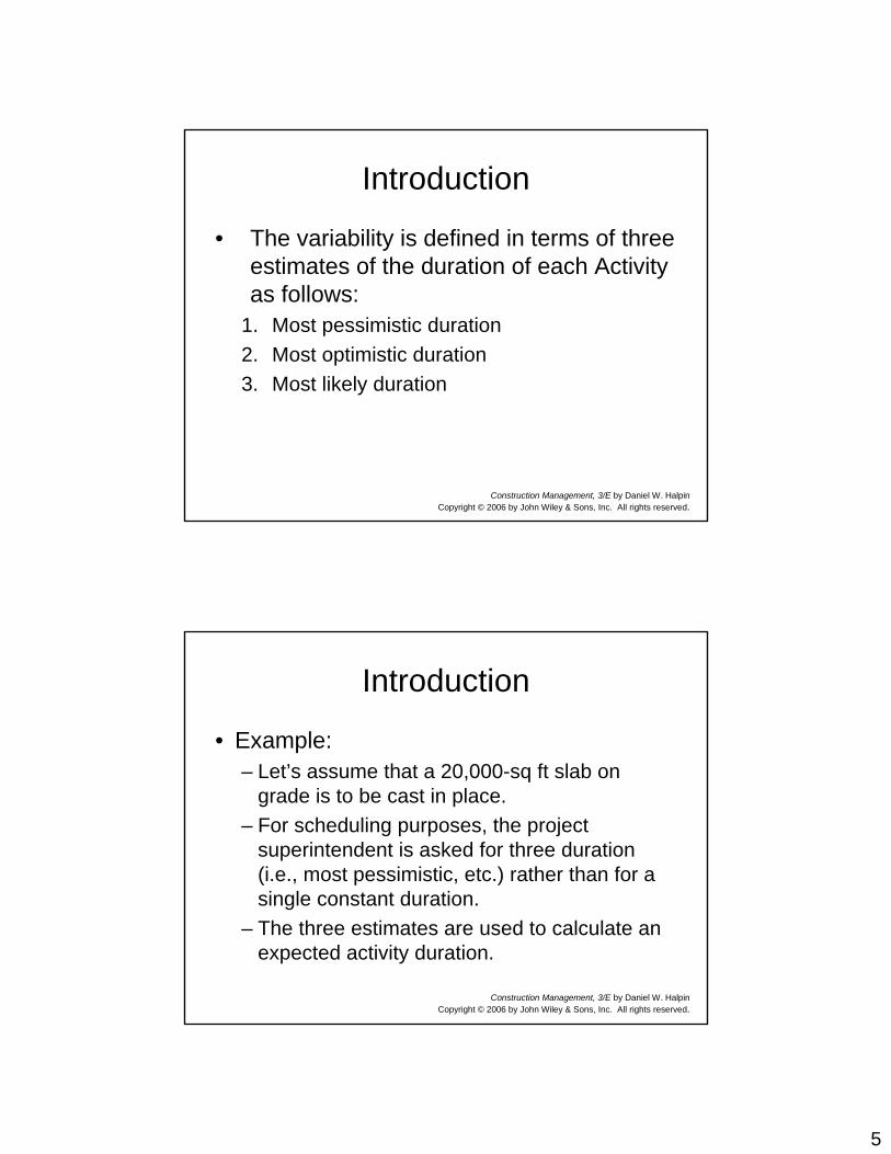
• The variability is defined in terms of three estimates of the duration of each Activity as follows:
1. Most pessimistic duration2. Most optimistic duration3. Most likely duration
Construction Management, 3/E by Daniel W. HalpinCopyright © 2006 by John Wiley & Sons, Inc. All rights reserved.
Introduction
• Example:– Let’s assume that a 20,000-sq ft slab on
grade is to be cast in place.– For scheduling purposes, the project
superintendent is asked for three duration (i.e., most pessimistic, etc.) rather than for a single constant duration.
– The three estimates are used to calculate an expected activity duration.
6
Construction Management, 3/E by Daniel W. HalpinCopyright © 2006 by John Wiley & Sons, Inc. All rights reserved.
Introduction
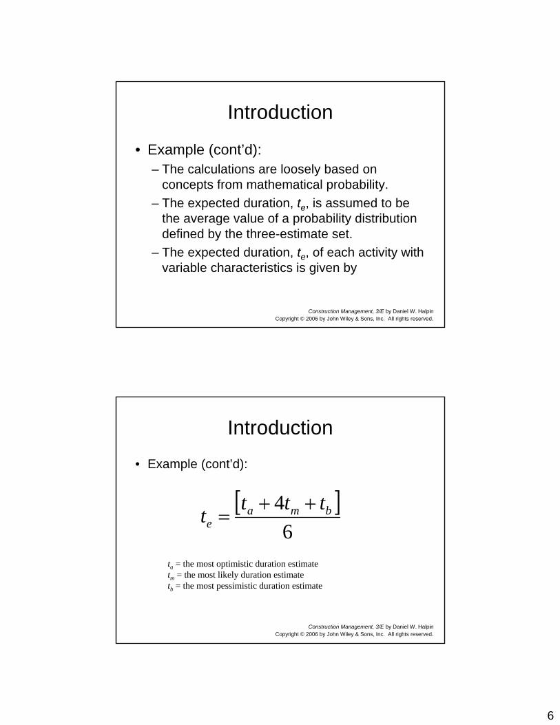
• Example (cont’d):– The calculations are loosely based on
concepts from mathematical probability.– The expected duration, te, is assumed to be
the average value of a probability distribution defined by the three-estimate set.
– The expected duration, te, of each activity with variable characteristics is given by
Construction Management, 3/E by Daniel W. HalpinCopyright © 2006 by John Wiley & Sons, Inc. All rights reserved.
Introduction
• Example (cont’d):
[ ]6
4 bmae
tttt ++=
ta = the most optimistic duration estimatetm = the most likely duration estimatetb = the most pessimistic duration estimate
7
Construction Management, 3/E by Daniel W. HalpinCopyright © 2006 by John Wiley & Sons, Inc. All rights reserved.
Introduction
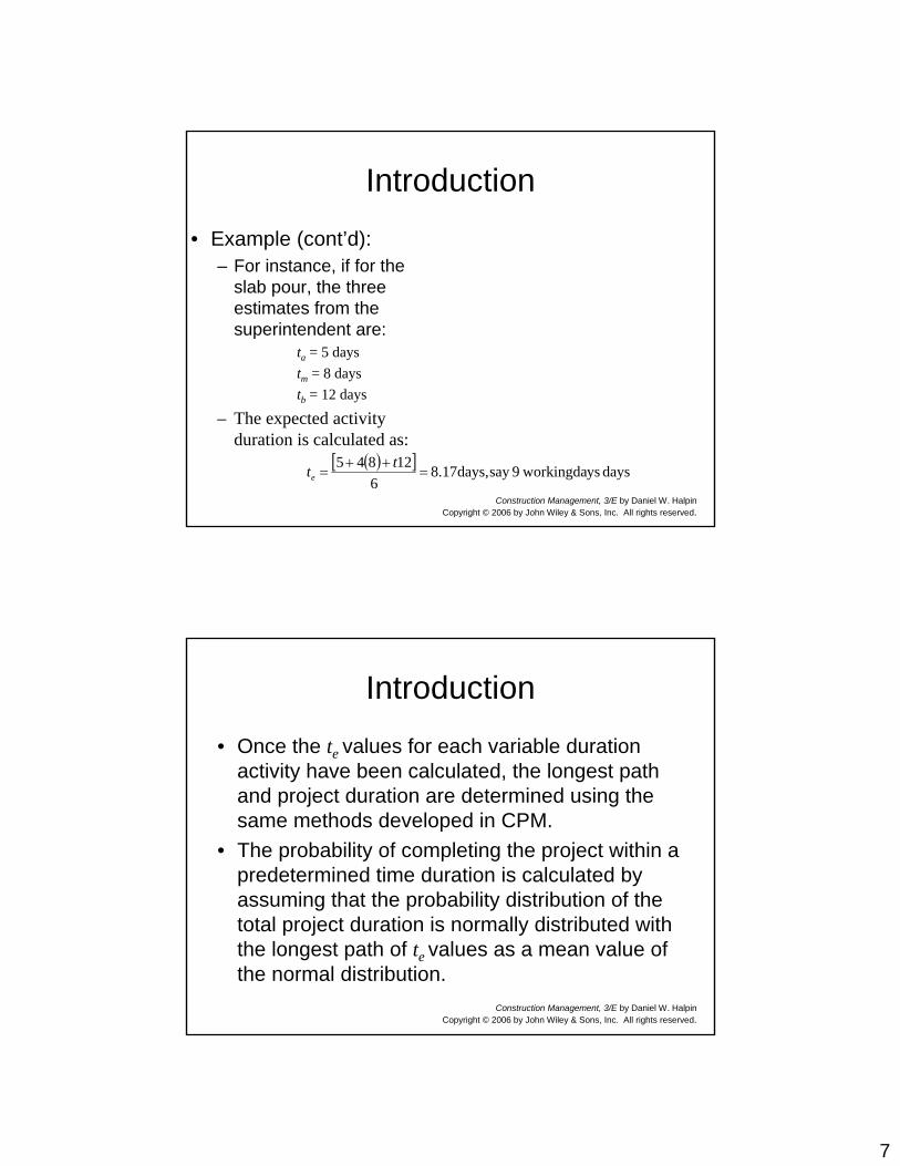
• Example (cont’d):– For instance, if for the
slab pour, the three estimates from the superintendent are:
ta = 5 daystm = 8 daystb = 12 days
– The expected activity duration is calculated as:
( )[ ] days ys workingda9say days,17.86
12845=
++=
tte
Construction Management, 3/E by Daniel W. HalpinCopyright © 2006 by John Wiley & Sons, Inc. All rights reserved.
Introduction
• Once the te values for each variable duration activity have been calculated, the longest path and project duration are determined using the same methods developed in CPM.
• The probability of completing the project within a predetermined time duration is calculated by assuming that the probability distribution of the total project duration is normally distributed with the longest path of te values as a mean value of the normal distribution.
8
Construction Management, 3/E by Daniel W. HalpinCopyright © 2006 by John Wiley & Sons, Inc. All rights reserved.
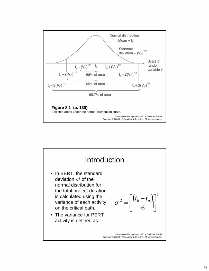
Introduction• The normal distribution is defined by its
mean value (i.e., in this case the value of the longest path through the net work) and the value, σ , which is so-called “standard deviation” of the distribution.
• The standard deviation of the distribution is a measure of how widely about the mean value the actual observed values are spread or distributed.
x
Construction Management, 3/E by Daniel W. HalpinCopyright © 2006 by John Wiley & Sons, Inc. All rights reserved.
Introduction
• Another parameter called the variance is the square of the standard deviation or σ2.
• It can be shown mathematically that 99.7% of the values of distributed variables will lie in a range defined by three standard deviations below the mean and three standard deviations above the mean (see the figure on the next slide)
9
Construction Management, 3/E by Daniel W. HalpinCopyright © 2006 by John Wiley & Sons, Inc. All rights reserved.
Figure 8.1 (p. 130)Selected areas under the normal distribution curve.
Construction Management, 3/E by Daniel W. HalpinCopyright © 2006 by John Wiley & Sons, Inc. All rights reserved.
Introduction
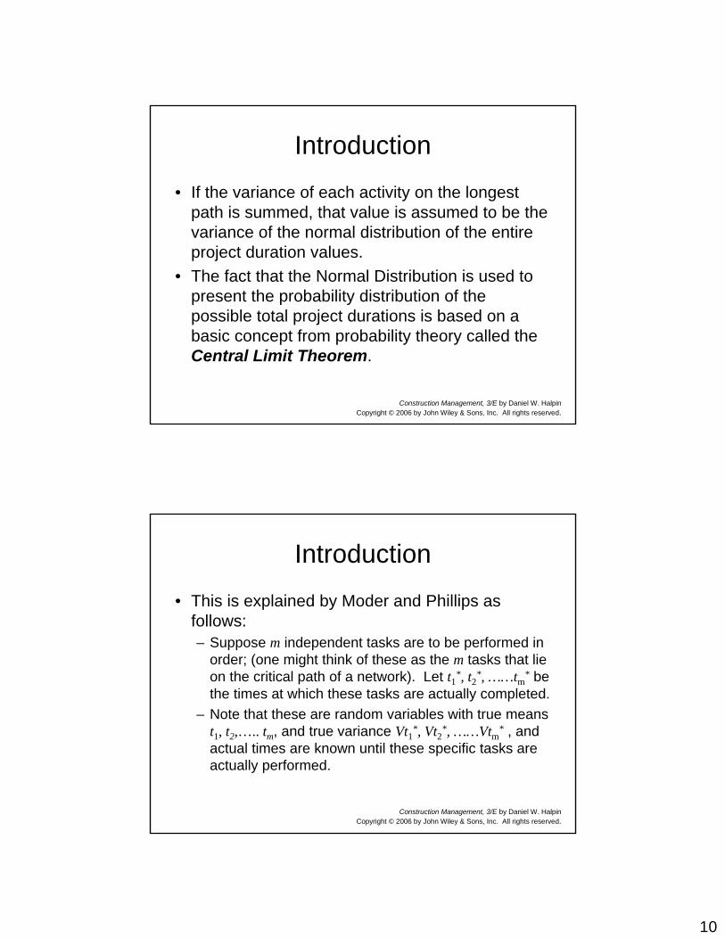
• In BERT, the standard deviation σ2 of the normal distribution for the total project duration is calculated using the variance of each activity on the critical path.
• The variance for PERT activity is defined as:
( ) 22
6 ⎥⎦⎤
⎢⎣⎡ −
= ab ttσ
10
Construction Management, 3/E by Daniel W. HalpinCopyright © 2006 by John Wiley & Sons, Inc. All rights reserved.
Introduction
• If the variance of each activity on the longest path is summed, that value is assumed to be the variance of the normal distribution of the entire project duration values.
• The fact that the Normal Distribution is used to present the probability distribution of the possible total project durations is based on a basic concept from probability theory called the Central Limit Theorem.
Construction Management, 3/E by Daniel W. HalpinCopyright © 2006 by John Wiley & Sons, Inc. All rights reserved.
Introduction
• This is explained by Moder and Phillips as follows:– Suppose m independent tasks are to be performed in
order; (one might think of these as the m tasks that lie on the critical path of a network). Let t1
*, t2*, ……tm
* be the times at which these tasks are actually completed.
– Note that these are random variables with true means t1, t2,….. tm, and true variance Vt1
*, Vt2*, ……Vtm
* , and actual times are known until these specific tasks are actually performed.
11
Construction Management, 3/E by Daniel W. HalpinCopyright © 2006 by John Wiley & Sons, Inc. All rights reserved.
Introduction• Now define T* to be the sum
of• And note that T* is also a
random variable and thus has a distribution. The Central Limit Theorem states that if m is large, say four or more, the distribution of T* is approximately normal with mean T and variance VT
* given by
**2
**mi tttT +++= …
Construction Management, 3/E by Daniel W. HalpinCopyright © 2006 by John Wiley & Sons, Inc. All rights reserved.
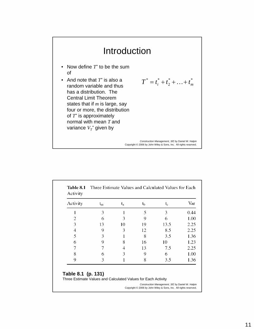
Table 8.1 (p. 131)Three Estimate Values and Calculated Values for Each Activity
12
Construction Management, 3/E by Daniel W. HalpinCopyright © 2006 by John Wiley & Sons, Inc. All rights reserved.
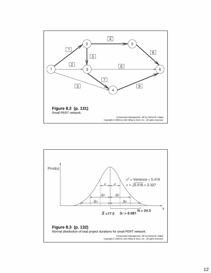
Figure 8.2 (p. 131)Small PERT network.
Construction Management, 3/E by Daniel W. HalpinCopyright © 2006 by John Wiley & Sons, Inc. All rights reserved.
Figure 8.3 (p. 132)Normal distribution of total project durations for small PERT network.
13
Construction Management, 3/E by Daniel W. HalpinCopyright © 2006 by John Wiley & Sons, Inc. All rights reserved.
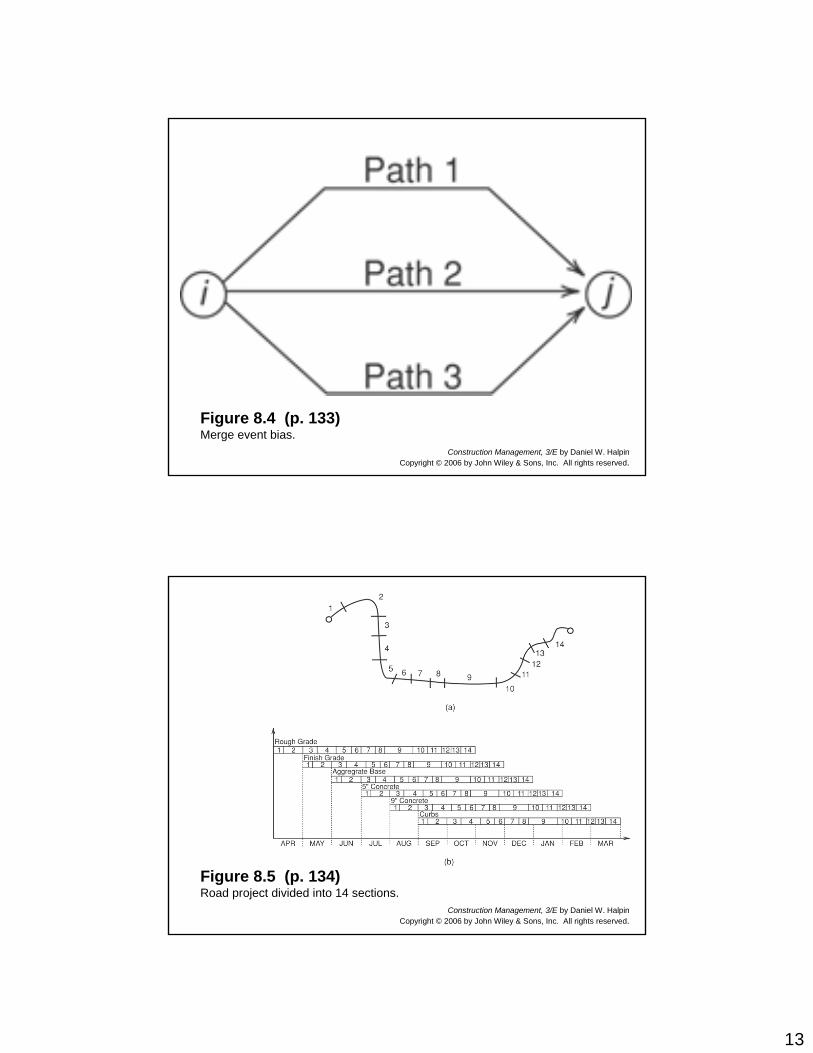
Figure 8.4 (p. 133)Merge event bias.
Construction Management, 3/E by Daniel W. HalpinCopyright © 2006 by John Wiley & Sons, Inc. All rights reserved.
Figure 8.5 (p. 134)Road project divided into 14 sections.
14
Construction Management, 3/E by Daniel W. HalpinCopyright © 2006 by John Wiley & Sons, Inc. All rights reserved.
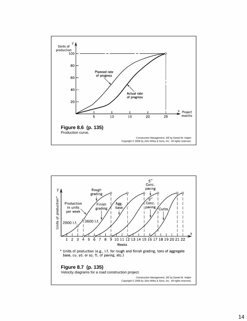
Figure 8.6 (p. 135)Production curve.
Construction Management, 3/E by Daniel W. HalpinCopyright © 2006 by John Wiley & Sons, Inc. All rights reserved.
Figure 8.7 (p. 135)Velocity diagrams for a road construction project.
15
Construction Management, 3/E by Daniel W. HalpinCopyright © 2006 by John Wiley & Sons, Inc. All rights reserved.
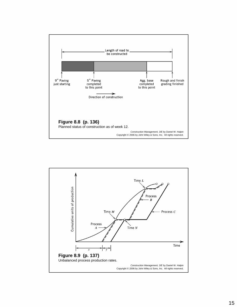
Figure 8.8 (p. 136)Planned status of construction as of week 12.
Construction Management, 3/E by Daniel W. HalpinCopyright © 2006 by John Wiley & Sons, Inc. All rights reserved.
Figure 8.9 (p. 137)Unbalanced process production rates.
16
Construction Management, 3/E by Daniel W. HalpinCopyright © 2006 by John Wiley & Sons, Inc. All rights reserved.
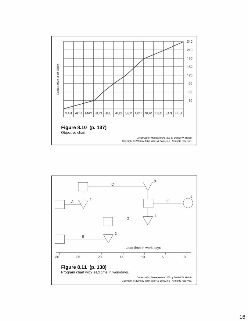
Figure 8.10 (p. 137)Objective chart.
Construction Management, 3/E by Daniel W. HalpinCopyright © 2006 by John Wiley & Sons, Inc. All rights reserved.
Figure 8.11 (p. 138)Program chart with lead time in workdays.
17
Construction Management, 3/E by Daniel W. HalpinCopyright © 2006 by John Wiley & Sons, Inc. All rights reserved.
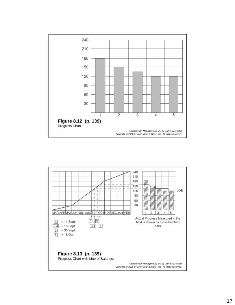
Figure 8.12 (p. 139)Progress Chart.
Construction Management, 3/E by Daniel W. HalpinCopyright © 2006 by John Wiley & Sons, Inc. All rights reserved.
Figure 8.13 (p. 139)Progress Chart with Line of Balance.
18
Construction Management, 3/E by Daniel W. HalpinCopyright © 2006 by John Wiley & Sons, Inc. All rights reserved.
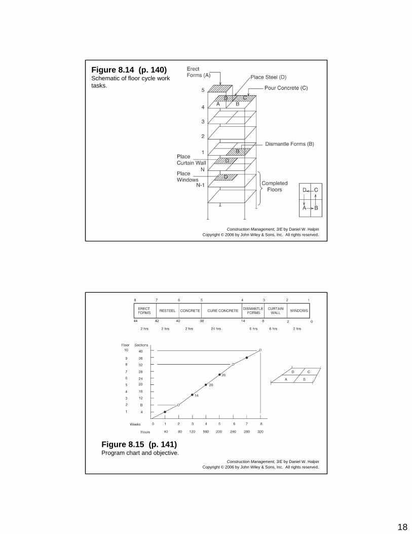
Figure 8.14 (p. 140)Schematic of floor cycle work tasks.
Construction Management, 3/E by Daniel W. HalpinCopyright © 2006 by John Wiley & Sons, Inc. All rights reserved.
Figure 8.15 (p. 141)Program chart and objective.
19
Construction Management, 3/E by Daniel W. HalpinCopyright © 2006 by John Wiley & Sons, Inc. All rights reserved.
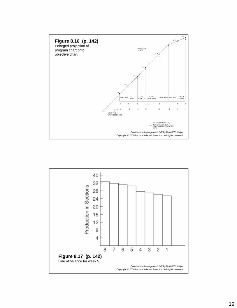
Figure 8.16 (p. 142)Enlarged projection of program chart onto objective chart.
Construction Management, 3/E by Daniel W. HalpinCopyright © 2006 by John Wiley & Sons, Inc. All rights reserved.
Figure 8.17 (p. 142)Line of balance for week 5.
20
Construction Management, 3/E by Daniel W. HalpinCopyright © 2006 by John Wiley & Sons, Inc. All rights reserved.
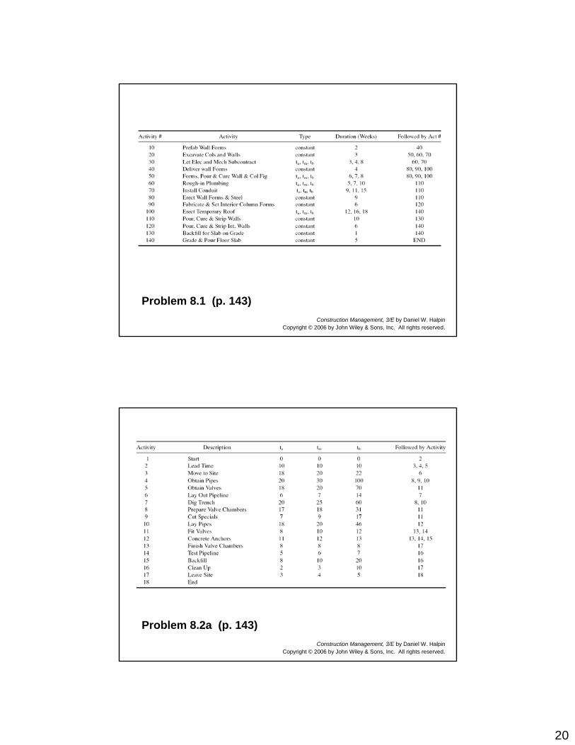
Problem 8.1 (p. 143)
Construction Management, 3/E by Daniel W. HalpinCopyright © 2006 by John Wiley & Sons, Inc. All rights reserved.
Problem 8.2a (p. 143)
21
Construction Management, 3/E by Daniel W. HalpinCopyright © 2006 by John Wiley & Sons, Inc. All rights reserved.
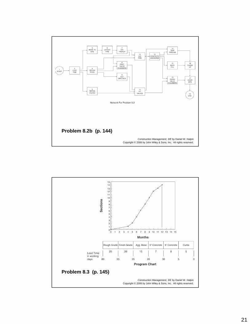
Problem 8.2b (p. 144)
Construction Management, 3/E by Daniel W. HalpinCopyright © 2006 by John Wiley & Sons, Inc. All rights reserved.
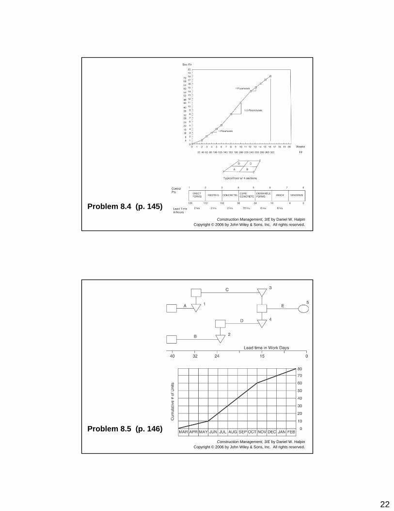
Problem 8.3 (p. 145)
22
Construction Management, 3/E by Daniel W. HalpinCopyright © 2006 by John Wiley & Sons, Inc. All rights reserved.
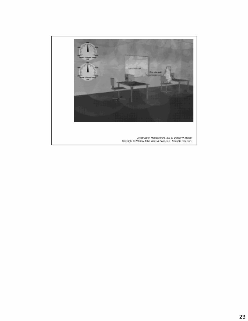
Problem 8.4 (p. 145)
Construction Management, 3/E by Daniel W. HalpinCopyright © 2006 by John Wiley & Sons, Inc. All rights reserved.
Problem 8.5 (p. 146)
23
Construction Management, 3/E by Daniel W. HalpinCopyright © 2006 by John Wiley & Sons, Inc. All rights reserved.


![[XLS] · Web view1 302 2 302 3 302 4 302 5 302 6 363 7 363 8 302 9 302 10 307 11 302 12 302 13 223244 14 302 15 302 16 224 17 302 18 302 19 302 20 302 21 302 22 23 24 25 26 302 27](https://img.pdfslide.us/doc/110x75/5b00c3a37f8b9a952f8d6104/xls-view1-302-2-302-3-302-4-302-5-302-6-363-7-363-8-302-9-302-10-307-11-302-12.jpg)