Embed Size (px)
Citation preview
ECO 153 INTRODUCTION TO QUANTITATIVE METHOD I Course Team Mr. O. E. Maku (Course Developer) – NOUN Dr. (Mrs.) G. A. Adesina-Uthman (Co-Developer)
– NOUN
NATIONAL OPEN UNIVERSITY OF NIGERIA
COURSE GUIDE
ECO 153 COURSE GUIDE
ii
National Open University of Nigeria Headquarters
14/16
Ahmadu
Bello
Way
Victoria
Island,
Lagos
E-mail: [email protected]
URL: www.nou.edu.ng Published by National Open University of Nigeria Printed 2014 Reprinted 2015, 2018 ISBN: 978-058-603-2 All Rights Reserved
Lagos Office
Plot 91, Cadastral Zone Nnamdi Azikiwe Expressway Jabi, Abuja
© 2018 by NOUN Press
ECO 153 COURSE GUIDE
iii
CONTENTS PAGE Introduction………………………………………………. iv Course Aims……………………………………………… iv Course Objectives………………………………………... iv Working through the Course……………………………... v Course Materials…………………………………………. v Study Units……………………………………………….. v Textbooks and References……………………………….. vi Assignment File………………………………………….. vi Tutor-Marked Assignment (TMA) ……………………….. vii Final Examination and Grading………………………….. vii Assessment………………………………………………. vii Presentation Schedule……………………………………. viii Course Overview…………………………………………. viii How to Get the Most from This Course…………………. ix Facilitators/Tutors and Tutorials…………………………. xi Summary………………………………………………….. xi

ECO 153 COURSE GUIDE
iv
INTRODUCTION ECO 153 - Introduction to Quantitative Method I is a three-unit course for 100Level students in National Open University of Nigeria. It comprises of 28 study units, subdivided into six modules. The materials have been developed with the Nigerian context in view by using simple and local examples. This course guide gives you an overview of the course. It also provides you with organisation and the requirement of the course. COURSE AIMS The course aims at introducing you to the quantitative method. This will be done by: • exposing you to the basic concept of real number system • explaining fraction, ratio, proportion and percentages to you • improving your knowledge about the various equations, functions
and change of subject of formulae • acquainting you with the basic simultaneous, linear and quadratic
equations • giving youan insight into the basic concepts, meaning and
classification of sets • making you understand the application of sets to managerial and
economic problems • introducing you to the meaning and types of sequence and
application of series and sequences to economics, business and finance
• explaining to you the meaning and types of matrices. COURSE OBJECTIVES To achieve the aims set above, there are some overall objectives. Each unit also has its objectives. These objectives will guide you in your study. They are usually stated at the beginning of each unit; and when you are through with studying the units, go back and read the objectives again. This would help you accomplish the task you have set to achieve. On successful completion of the course, you should be able to: • define and explain basic concepts of real number system • solve simple problems in fraction, ratio, proportion and
percentages

ECO 153 COURSE GUIDE
v
• demonstrate adequate skills in solving equations, functions and change of subject of formulae
• highlight the concepts, meaning and classification of sets • apply sets to managerial and economic problems • discuss the meaning and types of sequence • apply series and sequences to economics, business and finance • explain meaning and types of matrices. WORKING THROUGH THE COURSE To complete this course you are required to go through the study units and other related materials. You will also need to undertake practical exercises for which you need a pen, a notebook and other materials that will be listed in this guide. The exercises are to help you in understanding the basic concept and principles being taught in this course. At the end of each unit, you will be required to submit written assignments for assessment purpose. At the end of the course, you will write a final examination. COURSE MATERIALS The major materials you will need for this course are: 1. Course Guide 2. Study Units 3. Textbooks 4. Assignment File 5. Presentation Schedule STUDY UNITS There are six modules in this course broken into 28 study units: Module 1 Number and Numeration Unit 1 The Real Number System Unit 2 Fraction, Ratio, Proportion and Percentages Unit 3 Multiple and Lowest Common Multiples (LCM) Unit 4 Factors, Highest Common Factors (HCF) and Factorisation Unit 5 Indices, Logarithms and Surds Module 2 Equations and Formulae Unit 1 Equations, Functions and Change of Subject of Formulae Unit 2 Linear Equations and Linear Simultaneous Equations Unit 3 Quadratic Equations
ECO 153 COURSE GUIDE
vi
Unit 4 Simultaneous, Linear and Quadratic Equations Unit 5 Inequalities Module 3 Set Theory Unit 1 Meaning and Classification of Sets Unit 2 Set Notations and Terminologies Unit 3 Laws of Sets Operation Unit 4 Venn Diagrams Unit 5 Application of Sets to Managerial and Economic Problems Module 4 Sequence and Series Unit 1 Meaning and Types of Sequence Unit 2 Arithmetic Progression (AP) Unit 3 Geometric Progression (GP) Unit 4 Application of Series and Sequences to Economics, Business and Finance Module 5 Polynomial and Binomial Theorems Unit 1 Meaning and Scope of Polynomials Unit 2 Remainders’ and Factors Theorems Unit 3 Partial Fractions Unit 4 Binomial Expansions Unit 5 Factorials, Permutation and Combination Module 6 Matrices Unit 1 Meaning and Types of Matrices Unit 2 Matrix Operations Unit 3 Determinant of Matrices Unit 4 Inverse of Matrices and Linear Problems TEXTBOOKS AND REFERENCES Certain books are recommended in this course. You may wish to purchase or accessthem for further reading or practices. ASSIGNMENT FILE An assignment file and a marking scheme will be made available to you. In this file,you will find all the details of the work, you must submit to your tutor for marking.The marks you obtain from these assignments will count towards the final mark youobtain for this course. Further
ECO 153 COURSE GUIDE
vii
information on assignment will be found in the Assignment File itself and later in this Study Guide. TUTOR-MARKED ASSIGNMENT (TMA) You will need to submit a specific number of Tutor-Marked Assignment (TMA).Every unit in this course has a TMA. You will be assessed on fourof them, but the best three (out of the fourmarked) will be recorded. The total marks for the best three TMAs will be 30percent of your total work.Assignment questions for the unit in this course are contained in the Assignment File.When you have completed each assignment, send it, together with the TMA form to your tutor. Make sure each assignment reach your tutoron or before the deadline for submission. If for any reason, you cannot complete yourwork on time, contact your tutor to discuss the possibility of an extension. Extensionwill not be granted after due date, unless under exceptional circumstances. FINAL EXAMINATION AND GRADING The final examination for ECO 153 will be of three hours duration. All areas of thecourse will be examined. Find time to study and revise the unit all over before yourexamination. The final examination will attract 70 percent of the total course grade.The examination shall consist of questions which reflect the types of Self-Assessment Exercise and Tutor-Marked Assignment you have previously come across. Allareas of the course will be assessed. You are advised to revise the entire course afterstudying the last unit before you sit for the examination. You will also find it useful toreview your TMAs and the comments of your tutor on them beforethe final examination. ASSESSMENT There are two types of the assessment for this course. First is the tutor-marked assignments; second, the written examination. In attempting the assignments, you are expected to apply information, knowledge and techniques gathered during the course. The assignments must be submitted to your tutor for formal assessment in accordance with the deadlines stated in the Presentation Schedule and the Assignments File. The work you submit to your tutor for assessment will count for 30 % of your total course mark. At the end of the course, you will need to sit for a final written examination of three hours' duration. This examination will also count for 70% of your total course mark.
ECO 153 COURSE GUIDE
viii
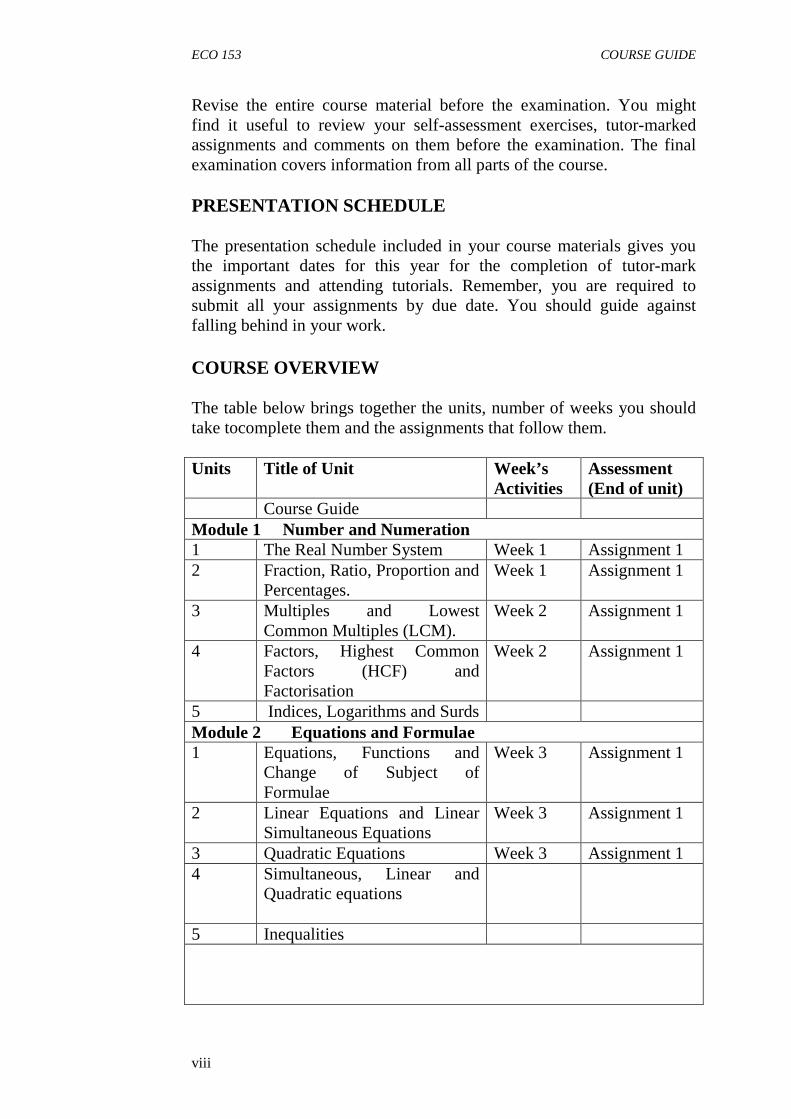
Revise the entire course material before the examination. You might find it useful to review your self-assessment exercises, tutor-marked assignments and comments on them before the examination. The final examination covers information from all parts of the course. PRESENTATION SCHEDULE The presentation schedule included in your course materials gives you the important dates for this year for the completion of tutor-mark assignments and attending tutorials. Remember, you are required to submit all your assignments by due date. You should guide against falling behind in your work. COURSE OVERVIEW The table below brings together the units, number of weeks you should take tocomplete them and the assignments that follow them. Units Title of Unit Week’s
Activities Assessment (End of unit)
Course Guide Module 1 Number and Numeration 1 The Real Number System Week 1 Assignment 1 2 Fraction, Ratio, Proportion and
Percentages. Week 1 Assignment 1
3 Multiples and Lowest Common Multiples (LCM).
Week 2 Assignment 1
4 Factors, Highest Common Factors (HCF) and Factorisation
Week 2 Assignment 1
5 Indices, Logarithms and Surds Module 2 Equations and Formulae 1 Equations, Functions and
Change of Subject of Formulae
Week 3 Assignment 1
2 Linear Equations and Linear Simultaneous Equations
Week 3 Assignment 1
3 Quadratic Equations Week 3 Assignment 1 4 Simultaneous, Linear and
Quadratic equations
5 Inequalities
ECO 153 COURSE GUIDE
ix
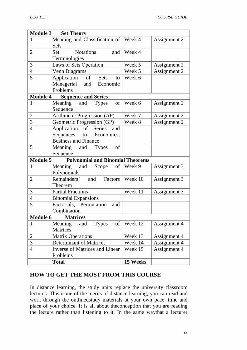
Module 3 Set Theory 1 Meaning and Classification of
Sets Week 4 Assignment 2
2 Set Notations and Terminologies
Week 4
3 Laws of Sets Operation Week 5 Assignment 2 4 Venn Diagrams Week 5 Assignment 2 5 Application of Sets to
Managerial and Economic Problems
Week 6
Module 4 Sequence and Series 1 Meaning and Types of
Sequence Week 6 Assignment 2
2 Arithmetic Progression (AP) Week 7 Assignment 2 3 Geometric Progression (GP) Week 8 Assignment 2 4 Application of Series and
Sequences to Economics, Business and Finance
5 Meaning and Types of Sequence
Module 5 Polynomial and Binomial Theorems 1 Meaning and Scope of
Polynomials Week 9 Assignment 3
2 Remainders’ and Factors Theorem
Week 10 Assignment 3
3 Partial Fractions Week 11 Assignment 3 4 Binomial Expansions 5 Factorials, Permutation and
Combination
Module 6 Matrices 1 Meaning and Types of
Matrices Week 12 Assignment 4
2 Matrix Operations Week 13 Assignment 4 3 Determinant of Matrices Week 14 Assignment 4 4 Inverse of Matrices and Linear
Problems Week 15 Assignment 4
Total 15 Weeks HOW TO GET THE MOST FROM THIS COURSE In distance learning, the study units replace the university classroom lectures. This isone of the merits of distance learning; you can read and work through the outlinedstudy materials at your own pace, time and place of your choice. It is all about theconception that you are reading the lecture rather than listening to it. In the same waythat a lecturer
ECO 153 COURSE GUIDE
x
might give you some reading to do, the study units contain instructionson when to read your set of books or other materials and practice some practicalquestions. Just as a lecturer might give you an in-class exercise or quiz, your studyunits provide exercises for you to do at appropriate point in time. Each of the studyunits follows a common format. The first item is an introduction to the subject matterof the unit and how a particular unit is integrated with the other units and the course asa whole. Followed by this is a set of objectives. These objectives let you know whatyou should be able to do at the end of each unit. These objectives are meant to guideyou and assess your understanding of each unit. When you have finished the units,you must go back and check whether you have achieved the objectives. If youcultivate the habit of doing this, you will improve your chances of passing the course.The main body of the unit guides you through the required reading from other sources.This will usually be either from your set books or from your course guides. Thefollowing is a practical strategy for working through the course. Always rememberthat your tutor’s job is to help you. When you need his assistance, do not hesitate tocall and ask your tutor to provide it. Follow the under-listed pieces of advicecarefully:- 1) Study this Course Guide thoroughly; it is your foremost
assignment. 2) Organise a Study Schedule: refer to the course overview for more
details. Notethe time you are expected to spend on each unit and how the assignmentsrelate to the units.
3) Having created your personal study schedule, ensure you adhere strictly to it.The major reason that students fail is their inability to work along with theirstudy schedule and thereby getting behind with their course work. If you havedifficulties in working along with your schedule, it is important you let yourtutor know.
4) Assemble the study material. Information about what you need for a unit isgiven in the ‘overview’ at the beginning of each unit. You will almost alwaysneed both the study unit you are working on and one of your set books on yourdesk at the same time.
5) Work through the study unit. The content of the unit itself has been arranged toprovide a sequence you will follow. As you work through the unit, you will beinstructed to read sections from your set books or other articles. Use the unit toguide your reading.
6) Review the objectives for each unit to be informed that you have achievedthem. If you feel uncertain about any of the objectives, review the studymaterial or consult your tutor.
7) When you are sure that you have achieved the objectives of a unit, you can thenstart on the next unit. Proceed unit by unit through the course and try to spaceyour study so that you keep yourself on schedule.

ECO 153 COURSE GUIDE
xi
8) When you have submitted an assignment to your tutor for marking, do not waitfor its return before starting on the next unit. Keep to your schedule. You arestrongly advised to consult your tutor as soon as possible if you have anychallenges or questions.
9) After completing the last unit, review the course and prepare yourself for thefinal examination. Check that you have achieved the objectives of the units(listed at the beginning of each unit) and the course objective (listed in thisCourse Guide).
10) Keep in touch with your study centre. Up-to-date course information will beconstantly made available for you there.
FACILITATORS/TUTORS AND TUTORIALS There are ten hours of tutorials provided in support of this course. You will be notifiedof the dates, times and location of these tutorials, together with the name and phonenumber of your tutor; as soon as you are allocated a tutorial group. Your tutor willgrade and comment on your assignments, keep a close watch on your progress and onany difficulties you might encounter and provide assistance to you during the course.You must mail your tutor-marked assignment to your tutor well before the due date(at least two working days are required). They will be marked by your tutor andreturned to you as soon as possible.Do not hesitate to contact your tutor by telephone, e-mail or personal discussions ifyou need help. The following might be circumstances in which you would find helpnecessary. Contact your tutor if you: i. do not understand any part of the study unit ii. have difficulty/difficulties with the self-assessment exercise(s) iii. have a question or problem with an assignment with your
tutor’scomments on any assignment or with the grading of an assignment.
You are advised to ensure that you attend tutorials regularly. This is the onlyopportunity to have a face to face contact with your tutor and ask questions. You canraise any problem encountered in the course of study. To gain the maximum benefitfrom course tutorials, prepare a question list before attending them and ensure youparticipate maximally and actively. SUMMARY This course guide gives an overview of what to expect in the course of this study.ECO 103 - Introduction to Quantitative Method I introduces you to the basic concept of real number system; fraction,

ECO 153 COURSE GUIDE
xii
ratio, proportion and percentages;improve knowledge about the various equations, functions and change of subject of formulae; acquaint you with the basic simultaneous, linear and quadratic equations; giveyou insight into the basic concepts, meaning and classification of sets; makes you understand application of sets to managerial and economic problems; introduce you to the meaning and types of sequence and application of series and sequences to economics, business and finance; andmeaning and types of matrices. It draws your attention to the use of simple and lucid statistical issues in solving day-to-day economic and business related problems. The use of simple instructional languagehas been adequately considered in preparing the course guide.
CONTENTS PAGE Module 1 Number and Numeration…………………. 1 Unit 1 The Real Number System………………...... 1 Unit 2 Fraction, Ratio, Proportion and Percentages…………………………………. 6 Unit 3 Multiple and Lowest Common Multiples (LCM)…………………………… 21 Unit 4 Factors, Highest Common Factors (HCF) and Factorisation…………… 26 Unit 5 Indices, Logarithms and Surds…………....... 32 Module 2 Equations and Formulae………………….. 44 Unit 1 Equations, Functions and Change of Subject of Formulae……………………... 44 Unit 2 Linear Equations and Linear Simultaneous Equations……………………. 53 Unit 3 Quadratic Equations………………………... 61 Unit 4 Simultaneous, Linear and Quadratic Equations………………………………….... 72 Unit 5 Inequalities…………………………………. 76 Module 3 Set Theory………………………………..... 83 Unit 1 Meaning and Classification of Sets………... 83 Unit 2 Set Notations and Terminologies………….. 89 Unit 3 Laws of Sets Operation…………………….. 97 Unit 4 Venn Diagrams……………………………… 103 Unit 5 Application of Sets to Managerial and Economic Problems…………………..... 112 Module 4 Sequence and Series……………………….. 124 Unit 1 Meaning and Types of Sequence…………… 124 Unit 2 Arithmetic Progression (AP)………………... 130 Unit 3 Geometric Progression (GP)………………... 138 Unit 4 Application of Series and Sequences to Economics, Business and Finance………. 144
MAIN COURSE
Module 5 Polynomial and Binomial Theorems……… 153 Unit 1 Meaning and Scope of Polynomials………… 153 Unit 2 Remainders’ and Factors Theorem………….. 160 Unit 3 Partial Fractions……………………………… 171 Unit 4 Binomial Expansions………………………… 183 Unit 5 Factorials, Permutation and Combination…… 188 Module 6 Matrices……………………………………… 198 Unit 1 Meaning and Types of Matrices……………… 198 Unit 2 Matrix Operations…………………………….. 208 Unit 3 Determinant of Matrices……………………… 223 Unit 4 Inverse of Matrices and Linear Problems……. 232
ECO 153 MODULE 1
1
MODULE 1 NUMBER AND NUMERATION Unit 1 The Real Number System Unit 2 Fraction, Ratio, Proportion and Percentages Unit 3 Multiples and Lowest Common Multiples (LCM) Unit 4 Factors, Highest Common Factors (HCF) and Factorisation Unit 5 Indices, Logarithms and Surds UNIT 1 THE REAL NUMBER SYSTEM CONTENTS
1.0 Introduction 2.0 Objectives 3.0 Main Content 3.1 General Overview 3.2 Real Number System (Integers, Rational Numbers,
Irrational Numbers, Imaginary Numbers) 4.0 Conclusion 5.0 Summary 6.0 Tutor-Marked Assignment 7.0 References/Further Reading 1.0 INTRODUCTION In this unit, we will begin this course by introducing the concept of real number system. We will also study the various component of the real number system such as integers, rational number irrational numbers, fractions, decimals and imaginary numbers. Equations and variables are the essential ingredients of mathematical expressions or models. The values economic variables take are usually numerical, there is need to start discussion on this study with the concept of number system. We will find out the relevance of numbers to mathematical analyses as well as the different forms of number list that make up the real number system. 2.0 OBJECTIVES At the end of the unit, you should be able to: • explain the concept “numbers” • identify the relevance of number system in quantitative analyses • outline various forms of numbers in the real number system with
examples
ECO 153 INTRODUCTION TO QUANTITATIVE METHOD I
2
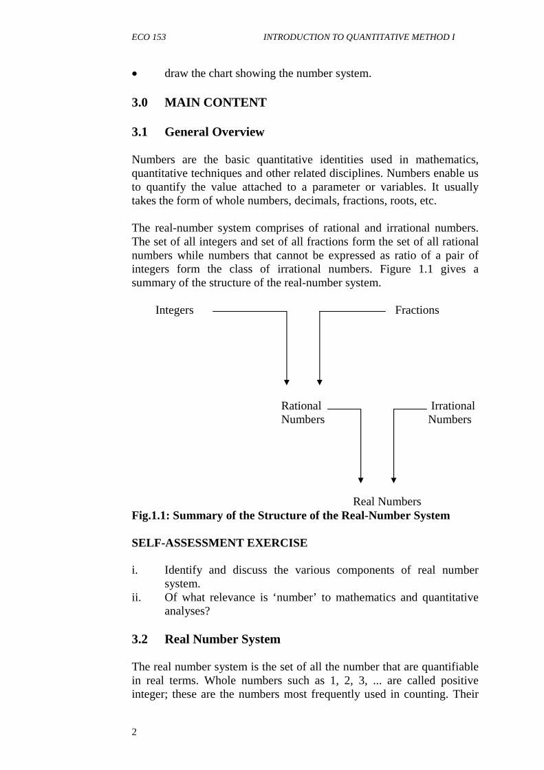
• draw the chart showing the number system. 3.0 MAIN CONTENT 3.1 General Overview Numbers are the basic quantitative identities used in mathematics, quantitative techniques and other related disciplines. Numbers enable us to quantify the value attached to a parameter or variables. It usually takes the form of whole numbers, decimals, fractions, roots, etc.
The real-number system comprises of rational and irrational numbers. The set of all integers and set of all fractions form the set of all rational numbers while numbers that cannot be expressed as ratio of a pair of integers form the class of irrational numbers. Figure 1.1 gives a summary of the structure of the real-number system. Integers Fractions Rational Irrational
Numbers Numbers
Real Numbers Fig.1.1: Summary of the Structure of the Real-Number System SELF-ASSESSMENT EXERCISE i. Identify and discuss the various components of real number
system. ii. Of what relevance is ‘number’ to mathematics and quantitative
analyses? 3.2 Real Number System The real number system is the set of all the number that are quantifiable in real terms. Whole numbers such as 1, 2, 3, ... are called positive integer; these are the numbers most frequently used in counting. Their

ECO 153 MODULE 1
3
negative counterparts -1, -2, -3 ... are called negative integers. The negative integers are used to indicate sub-zero quantities e.g. temperature (degree). The number 0 (Zero), on the other hand is neither a positive nor a negative integer and in that sense unique. Sometimes, it is called a neutral number. A set of negative and positive whole numbers (integers) can be presented with the use of number line as follows: NEUTRAL NUMBER NEGATIVE POSITIVE INTEGERS INTEGERS -∞ -3 -2 -1 1 2 3 ∞ 0 Fig. 1.2:Real Number System Sometimes, positive integers, negative integers and zero are lumped together into a single category, referring to them collectively as the set of all integers.
Integers, of course, do not exhaust all the possible whole number. Factors such as 2/3,
5/4, 7/8, ½, also fall within the number line showing
the members of integers. Negative fractions such as -1/2, -7/8, -
5/4 are also components of negative integers. In other words, integers are set of positive or negative whole numbers as well as the set of positive or negative fraction, zero inclusive. The common property of all fractional numbers is that each is expressible as a ratio of two integers; thus fractions qualify for the class of rational numbers (in this usage, rational means ratio-nal). However, integers are also rational because any integer, n can be considered as the ratio n/1. The set of all integers and the set of all fractions together form the set of all rational numbers.
Numbers that are not rational are termed irrational numbers. They are numbers that cannot be expressed as a ratio of a pair of integers. One example of irrational number is √2 = 1.4142..., which is a non repeating, non terminating and recurring decimal. Another common example is ∏ = 22/7 = 3.1415 (representing the ratio of the circumference of any circle to its diameter).
ECO 153 INTRODUCTION TO QUANTITATIVE METHOD I
4
Each irrational number can also be placed in a number line lying between two rational numbers, just as fraction fills the gaps between the integers. The result of this filling – in the process gives a large quantum of numbers; all of which are so called “real numbers”. The set of real numbers is denoted by symbol R. When the set of R is displaced on a straight line (an extended ruler), we refer to the line as the real line.
At the extreme opposite of real numbers are the set of number are the set of numbers that are not real. They are called imaginary numbers. The common examples of imaginary numbers are the square root of negative numbers e.g. √−7,√−4,√−25,√−140, etc. SELF-ASSESSMENT EXERCISE
Classify each of the following numbers into integers, irrational number and imaginary numbers: (i) 5/8 (ii) √−9 (iii) √9 (iv) √23 (v) -20 (vi) 32/5 (vii) ℮ = 2.71828… (viii) -7 (ix) -(√8) (x) 17/7 4.0 CONCLUSION
Numbers are generally quantifiable variables used in mathematics to describe the magnitude of quantities. There are two broad classifications of numbers namely: real numbers and imaginary numbers. While real number comprises of positive and negative whole numbers, positive and negative fractions and irrational numbers, the imaginary numbers are the extreme opposite of real numbers. They are number that cannot be placed on the real line. Basic mathematical skills and technique starts from numbers and numerations since numbers especially figures are the basis of counting, quantifying and carrying out mathematical operations. 5.0 SUMMARY
In mathematics and quantitative analysis, the roles play by numbers in all its ramifications cannot be over-emphasised. For this reason, every arithmetic class starts with the counting and writing of whole numbers. As students of arithmetic moves to mathematics class, other forms of numbers such as negatives numbers, fractions, decimals, irrational numbers and, imaginary numbers are introduced. Therefore, as the basis of numerical and quantitative analyses, numbers and numeration take the foremost and essential attention at all levels. 6.0 TUTOR-MARKED ASSIGNMENT
1. What are numbers? 2. What are the relevance of numbers to mathematics and
quantitative analyses?

ECO 153 MODULE 1
5
3. What are real numbers? 4. What are the components of real numbers? 5. Give two examples of each of the following types of numbers:
a) Positive integers b) Negative integers c) Fractions d) Irrational numbers e) Imaginary numbers.
7.0 REFERENCES/FURTHER READING
Alfa, C. C. (1984). Fundamental Methods of Mathematical Economics.(3rded.). New York: McGraw-Hill Inc.
Karl, J. S. (1990). Mathematics for Business. US: Win C. Brown
Publishers. Lucey, T. (1988). Quantitative Techniques: An Introductional Manual.
(3rded.). London: ELBS/DP Publications.

ECO 153 INTRODUCTION TO QUANTITATIVE METHOD I
6
UNIT 2 FRACTION, RATIO AND PROPORTION CONTENTS 1.0 Introduction 2.0 Objectives 3.0 Main Content 3.1 General Overview 3.2 Fractions 3.2.1 Forms of Fraction 3.2.2 Equivalent Fractions 3.2.3 Addition and Subtraction of Fractions 3.2.4 Multiplication of Fractions 3.2.5 Division of Fractions
3.2.6 Mixed Operation 3.2.7 Change of Fraction to Decimal, Ratio and Percentage 3.2.8 Application of Fraction to Business Management/Economics
3.3 Ratio 3.4 Proportion 3.5 Percentages 4.0 Conclusion 5.0 Summary 6.0 Tutor-Marked Assignment 7.0 References/Further Reading 1.0 INTRODUCTION
In this unit, we will study the breakdown of a whole numbers into fractions, ratio and proportion. The division of a whole component into divisions is a day to day phenomenon. Individuals income are divided into ratio, fraction or proportion to ensure that all the basic needs are met, the same thing applies to the business organisations’ profit and the governments resources, income and wealth. Therefore, it is important to study the fractional parts of a whole as it affects sharing components in terms of ratio and proportion. In the previous unit, fractions have been identified as a component of real numbers which forms between the whole number lines. Therefore, in this unit, we shallexamine the components of rational number known as fraction which is also expressed in ratio, proportion or percentages.
ECO 153 MODULE 1
7
2.0 OBJECTIVES At the end of this unit, you should be able to: • identify the relationship between fraction, ratio, proportion and
percentages • convert fractions to ratio, proportion and percentages and vice
versa • perform simple mathematical problems involving fraction, ratio,
proportion and percentages • solve some practical problems involving fraction, ratio,
proportion and percentages. 3.0 MAIN CONTENT 3.1 General Overview
Mathematics is not limited to operation in whole numbers alone. Most often than none, proportion and fractions are used in mathematical analyses to demonstrate the possibilities of treating a unit into denominations or parts. For instance, an orange can be shared among four children equally so that each of them gets a quarter of the orange. If mathematics is limited to the study of whole numbers alone, it will be extremely difficult to share and divide resources among the constituents that own it.
A fraction is a small amount or proportion of a whole. Fractions are used to describe quantities which are less (smaller) than a whole unit. Expression of fraction is usually in the form of m/n e.g. 1/2,
3/5, 2/7,
2/3, etc., where “m” is the numerator and “n” is the denominator.
A ratio is a relationship between two or more magnitudes expressed in relative magnitudes. It compares the relative magnitudes which exist between certain quantities or values that are expressed in the same unit or are of the same kind. A ratio can also be described as a quotient of two mathematical expression expressed in the lowest term. Ratios are the same as fraction except that they are not expressed in numerators and denominators e.g. 2/3 = 2:3, 3/5 = 3:5, 2/7 = 2:7.
A proportion is simply an expression of the equation of two ratios. It is thus an equation which shows that one ratio is equal to another. It is also a method used to divide a given quantity in a given ratio. Proportion problems usually require finding the value of one of the missing terms. The solution require either the cross multiplication of the means and extreme (e.g. 3:6 = 1:2, the numbers 3 and 2 are called the
ECO 153 INTRODUCTION TO QUANTITATIVE METHOD I
8
extremeswhile 6 and 1 are called the means), or by solving for the value of an unknown in an equation.
A percentage is a fraction expressed in the unit of hundred e.g. 2/5 is a fraction which is equal to (2/5 x 100/1%) i.e. 40%. Therefore, 2/5 =2:5 =40:100 =40%. The quantity of a proportion from a whole when the whole is taken to have 100 units is called the percentage of the proportion from the whole.
SELF-ASSESSMENT EXERCISE With appropriate examples, demonstrate the relationship between fraction, ratio, proportion and percentages. 3.2 Fractions 3.2.1 Forms of Fraction
Fractions are of different types. Some of the types are: Proper Fraction: - This is a fraction which has its numerator smaller than the denominator e.g. ½, ¾, 3/5 etc.
Improper fraction: This is a fraction which has its denominator smaller than the numerator e.g. 3/2,
7/4, 9/5 etc.
Mixed Number: A mixed number is a fraction that has two portion; the whole number portion and the proper fraction portion e.g. 21/4,
12/5, 32/7
etc. it should be noted that mixed numbers can be expressed as improper fraction e.g. 21/4 = 9/4 (the value of 9 is obtained by multiplying 4 by 2 and adding 1), 12/5 = 7/5, 3
2/7 = 23/7 etc.
Complex Number: This is one in which the numerator or the denominator or both are either proper fraction, improper fraction or mixed numbers e.g.
2 3�4 5� ,2 ��
3 ��, �� x ���� x ��
���.
3.2.2 Equivalent Fractions When both numerator and denominator of a fraction are multiplied by the same number (except zero), another fraction is obtained. Likewise, when both the numerator and the denominator of a fraction are divided by the same number (except zero), another fraction of equal value is
ECO 153 MODULE 1
9
obtained. The fraction obtained in each of the cases is called the Equivalent Fraction. Example: Express the following fractions in their lowest possible equivalent/term.
(a) 3/9 (b) 8/12 (c) 4xy/12xy (d) ����������
(a) 3/9 = 1/3 (3 is the highest factor common to both numerator and denominator. Each of them is divided by 3 to obtain 1/3). (b) 8/12 = 2/3 (4 is the highest common factor) (c) 4xy/12yz = x/3z (4y is the highest common factor of both numerator and denominator, diving each by 4y gives x/3z).
(d) ���������� = ��� (16���ℎ�ℎ�ℎ���� ��������) From the above; 8/12 = 4/6 = 2/3 4xy = 4 x xx y = x 12yz 3 x 4 x y x z 3z 16x2y = 2 x 2 x 2 x 2 x xxxx y = x 32xy2 2 x 2 x 2 x 2 x 2 x xx y x y 2y
3.2.3 Addition and Subtraction of Fractions
When fractions have the same number as their denominators, their numerators can simply be added together or subtracted from one another, keeping their denominator constant.
e.g. (a) � + � = �
(b) � − � = � = ��
(c) �� + �� = �� = 1
(d) 2 �� + 3 �� = 5 �� = 5 + �� = 5 + 1 = 6
Where the denominators are different, the lowest common multiple is found first and the expression would then be simplified.
e.g (e) �� + �� + �� = �� ���� = ���� = 2 ���
ECO 153 INTRODUCTION TO QUANTITATIVE METHOD I
10
(f)2 �� + 1 �� = 3 ���� = 3 ���� = 3 + ���� = 3+1 ��� = 4 ��� (g)3 �� − 2 �� = 1 ���� = ��������� = � ��� = ����
Note: In the example (g) above, 6 minus 7 appears impossible, so the whole number 1 is borrowed, where 1 in this context equals to 12/12.
3.2.4 Multiplication of Fractions In multiplication, the numerators are multiplied by each other while the denominators are also multiplied with each other. It should be noted that when numbers are multiplied by each other, the result is a bigger number but when fraction are multiplied by each other, the result is a smaller number e.g.
2x2 = 4,3x3 = 9,4x8 = 32 12 x
12 = 1
4 ,13 x
13 = 1
9 , 12 �� 1
6 = 12 x
16 = 112
It should be noted that, when multiplication is to be carried out for mixed numbers, they (the mixed number) are converted to improper fraction before the multiplication.
e.g. 1 �� �2 �� �4 ��
= 75 � 52 � 9
2 = 634 = 1534
(Note '5' in both numerator and the denominator cancels each other out)
3.2.5 Division of Fractions In division of one fraction by other, the divisor is inverted (turned upside down) and then multiplied by individual i.e. the dividend is multiplied by the reciprocal of the divisor
e.g. �� ÷ �� ��� �ℎ����������ℎ�� �� �ℎ���������.
13 x
32 = 1
2
78 ÷ 5 = 78 x 15 = 7
40
ECO 153 MODULE 1
11
When dealing with mixed numbers, the dividend and the divisor are first expressed in improper fraction and the principle of division is then applied. e.g.
712 ÷ 313 = 152 ÷ 103 = 15
2 x 310 = 94
4��2�� ÷ 3�
2� = 4��2�� x 3�2� = 3��
3.2.6 Mixed Operation
By mixed operation, we mean a fraction that involves the mixture of operations (addition, subtraction, multiplication, division). In such situation, the rule of precedence is followed and this is summarised by the word “BODMAS” which gives the order as follows:
B = Bracket O = Of D = Division M = Multiplication A = Addition S = Subtraction
This implies that in mixed operation, attention should first be based on bracket, followed by ‘of’, then division before multiplication. Addition signs are evaluated before the subtraction.
E.g. Simplify (i) 1 � x �� − 3 �� + 2 �� ÷ �� (ii)
�� �� �2 �� − 1 ��
(iii)��������������
(i) 1 � x �� − 3 �� + 2 �� ÷ �� = ��� x �� − ��� + ��� x �� = �� − ��� + ��
= ������������
= 18145 = 2 4145
(ii) �� �� �2 �� − 1 �� = �� �� �1 − ����� �
= �� �� ��������� �
= �� �� �������� �
ECO 153 INTRODUCTION TO QUANTITATIVE METHOD I
12
= �� �� ������
= �� x ���� = ����
(iii) �������������� = �
����
��� ��
�
= �����
�����
= �� ÷ ��� = �� x ���
= 225196 = 1 59196
3.2.7 Change of Fraction to Decimal, Ratio and Percentage
Fraction are converted to decimal by dividing the numerator by the denominator while fraction are converted to percentage by multiplying the fraction by 100 and presenting the answer in percentage (%). The conversion of fraction to ratio only requires the presentation of the numerator as the ratio of the denominator.
E.g. Convert (a) �� (b) 2 �� to
(i) Decimal (ii) Ratio
(iii) Percentage
(a) �� = 2 ÷ 5 = 0.4!"�� ��#
25 = 2 ∶ 5!����#
25 = 2
5 x1001 % = 40%!$��������#
(b) 2 �� = � = 2.25!"�� ��# 214 = 94 = 9 ∶ 4!����#
214 = 94 x
1001 = 225%!$���������#
3.2.8 Application of Fraction to Business
Management/Economics The addition, subtraction, multiplication and division of fraction can be applied in business management and economics in areas involving the determination of total cost of items, discounts, deductions from salaries,

ECO 153 MODULE 1
13
tax liabilities, unit cost of manufactured products or service rendered, return inwards, return outwards etc. Example 1: The total production cost of XYZ Company was N 3 million. Factory overhead amounted to N1 million and prime cost is N1.5 million. Other items of the cost amounted to N 50,000. Calculate the fraction of the total spent on other items. Solution %�������&��ℎ��" = '1 '3 = 1
3 $� ���� = '15 '3 = 12 (�ℎ���� = 1 − )13 + 12*
= 1 − ����� �
= 1 − 56 = 1
6
�� '500,000'3,000,000 = 16
Example 2: The total expenses of Ade and Olu Nigeria Limited in the year ended 31 December, 2004 was N180, 000. This consists of:
Wages and salaries N 50, 000 Selling and distributing expenses N 20,000 Insurance N 5,000 Rent N 30,000 Electricity N 35,000 Traveling and fueling N 35,000 Miscellaneous expenses N 5,000 What fractional part of the total is: (a) Rent (b) Insurance and electricity (c) Wages, salaries and rent
Solution
(a) +��� = ���,����� �,��� = �� (b) ,�-�������"��������� = ��,�������,����� �,��� = ���,����� �,��� = � (c) .���, �������"���� = ���,�������,����� �,��� = � �,����� �,��� = �
SELF-ASSESSMENT EXERCISE

ECO 153 INTRODUCTION TO QUANTITATIVE METHOD I
14
i. Change the following fractions to (i) percentages (ii) ratio (iii) decimal: (a) ½ (b) 2/3 (c) 3/5 (d) 1/3 (e) 5/2
ii. Simplify each of the following: (a) 23/4 + 32/5 – 11/3 (b) 31/5 + (22/5 ÷ 11/5) (c) 51/3 + (41/2 of 31/3 -1)
iii. Anambra, Imo and Ebonyi states decided to go into a joint venture business to produce some products at a large scale. Anambra provides 1/3 of the funds required for the investment. If Imo provides 2/3 of the remaining, what proportion or fraction of the investment is provided by Ebonyi state?
3.3 Ratio A ratio expresses the functional relationship between two or more magnitude. It can be described as a quotient stated in a linear lay out. For example: a/b = a:b. it should be noted that only quantities in the same unit or of the same kind can be expressed in ratio. Ratios are normally reduced to lowest terms, like fractions. Example 1 (a) What ratio of N20 is N5? (b) Express 3 hours as a ratio of 3 days. (c) What ratio of 2 hours is 45 minutes? (d) Express 200g as a ratio of 4kg. Solution (a) N5: N20
= 1:4 (b) 3hrs: 3days
3hrs: (3 x 24) hrs 3hrs: 72 hrs 1: 24
(c) 45mins: 2 hours 45mins: (2 x 60) mins 45mins: 120mins 9: 24 3: 8 (d) 200g: 4kg 200g: (4 x 1000)g 200g: 4000g 1: 20
ECO 153 MODULE 1
15
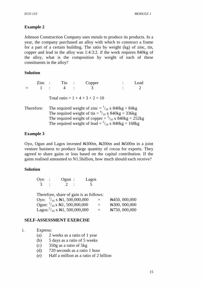
Example 2 Johnson Construction Company uses metals to produce its products. In a year, the company purchased an alloy with which to construct a frame for a part of a certain building. The ratio by weight (kg) of zinc, tin, copper and lead in the alloy was 1:4:3:2. if the work requires 840kg of the alloy, what is the composition by weight of each of these constituents in the alloy?
Solution
Zinc : Tin : Copper : Lead
= 1 : 4 : 3 : 2
Total ratio = 1 + 4 + 3 + 2 = 10
Therefore: The required weight of zinc = 1/10 x 840kg = 84kg The required weight of tin = 4/10 x 840kg = 336kg The required weight of copper = 3/10 x 840kg = 252kg The required weight of lead = 2/10 x 840kg = 168kg
Example 3 Oyo, Ogun and Lagos invested N300m, N200m and N500m in a joint venture business to produce large quantity of cocoa for exports. They agreed to share gains or loss based on the capital contribution. If the gains realised amounted to N1.5billion, how much should each receive? Solution Oyo : Ogun : Lagos 3 : 2 : 5
Therefore, share of gain is as follows: Oyo: 3/10 x N1, 500,000,000 = N450, 000,000 Ogun: 2/10 x N1, 500,000,000 = N300, 000,000 Lagos: 5/10 x N1, 500,000,000 = N750, 000,000
SELF-ASSESSMENT EXERCISE
i. Express: (a) 2 weeks as a ratio of 1 year (b) 5 days as a ratio of 5 weeks (c) 350g as a ratio of 5kg (d) 720 seconds as a ratio 1 hour (e) Half a million as a ratio of 2 billion
ECO 153 INTRODUCTION TO QUANTITATIVE METHOD I
16
ii. Danladi and Sons Limited made total sales of N50, 200 on a certain market day. Of this sales figure, sales of beans accounted for N32, 600. What is the ratio of beans sales to the total sales?
iii. Ade, Olu and Dayo share profits in a partnership business in the ratio 2:5:8. If the total profit realised is N30, 000,000. How much should each of them share?
3.4 Proportion
A proportion is simply an expression of the equivalence or equality of two ratios. It is a method used to divide a given quantity in a given ratio. Proportion techniques are useful in finding the missing value of a given set of ratio.
Example 1
2 : 3 = x : 12 = 10 : y = 6 : z. Find x, y and z Solution: To find the value of x, y and z, there is need to use a complete ratio of 2:3 in order to find the missing values. 2: 3 = x: 12 3 is multiplied by 4 to get 12, the same 4 should multiply 2 to get x Therefore, 2: 3 = (2 x 4): 12
2: 3 = 8: 12, therefore x = 8.
Likewise, 2: 3 = 10: y 2: 3 = (2 x 5): (3 x 5) 2: 3 = 10: 9, therefore y = 15.
Likewise, 2: 3 = 6: z 2: 3 = (2 x 3): (3 x 3) 2: 3 = 6: 9, therefore z = 9.
Example 2
It costs a company N200 to purchase 1 gallon of fuel. Of the delivery van of the company uses 30 gallons to travel 300km, how much would this company need to spend on fuel if only 100km is required to be traveled?
Solution
1 gallon cost N200 300km uses 30 gallons
Therefore, 1km uses (30/300) gallons A journey of 100km uses (30/300 x 100) gallons
ECO 153 MODULE 1
17
= 10 gallons. Since a gallon costs N200 Therefore, 10 gallons cost N200 x 10 = N2,000.
Example 3
It took 5 men 20 hours to clean up the warehouse of a certain company. How much time will be taken by 10 men doing the same work at the same rate?
Solution
5 men take 20 hours to do the work 1 man takes (20 x 5) hours = 100 hours to do the work. i.e. 10 men takes 20 x 5 10 = 10 hours to do the work. Example 4 If 250 labourers are needed to clean up the factory of a certain manufacturing companies having 50 machines. How many labourers will be needed if additional 40 similar machines are required? Solution
250 labourers needed for 50 machines i.e. 250/50labour need for 1 machine Additional 40 machines make the machine 90 in number i.e. Number of labourers required to clean up 90 machines = 250 x 90 50 = 5 x 90 = 450 labourers. SELF-ASSESSMENT EXERCISE i. Obiageli Industries Ltd earned N100, 000 as return on investment
of N500, 000. How much would be earned at the same rate of return on an investment of N50, 000?
ii. John Coy Limited produces certain products, each of which combines 12kg of lead with 15kg of copper. How many kg of lead will this product combine with 20kg of copper?
ECO 153 INTRODUCTION TO QUANTITATIVE METHOD I
18
iii. Andrew and Sons is an oil servicing company. It takes 9 engineers of the company 8 days to complete the servicing of an oil drilling equipment at the rig offshore. How many days will it take 6 engineers to complete the same work if working at the same rate?
iv. For selling an item for N900 a trader make a profit of 25%. What should the selling price be to make a profit of 30%?
3.5 Percentages Percentages refer to a ratio that equates the second number to 100. It is actually the number of parts that are taken out of a hundred parts. For instance, 60% (60 percent) means 60 out of a hundred or 60/100 or 6/10 or 3/5 or 3:5. Percentages can be easily converted to fraction, decimal or ratio. Example 1 Convert the following to percentages (a) 1/3 (b) ¼ (c) 2/5 Solution
(a) 1/3 = 1/3 x 100/1 = 33.33% (b) ¼ = ¼ x 100/1 = 25% (c) 2/5 = 2/5 x 100/1 = 40% Example 2 Change the following decimal fractions to percentage. (a) 0.65 (b) 0.43 (c) 1.95
Solution
(a) 0.65 = 0.65 x 100 = 65% (b) 0.43 = 0.43 x 100 = 43% (c) 1.95 = 1.95 x 100 = 195%
Example 3
Convert the following ratio to percentages. (a) 2 : 5 (b) 3 : 4 (c) 15 : 25
Solution
(a) 2 : 5 = 2/5 x 100 = 40% (b) 3 : 4 = 3/4 x 100 = 75% (c) 15 : 25 = 15/25 x 100 = 60%
Example 4

ECO 153 MODULE 1
19
A man bought an article for N20, 000 and sold it for N25,000. What is the percentage profit?
Solution Profit = Selling Price minus Cost price
% Profit = Profit x 100 Cost Price 1
= N25, 000 – N20, 000x 100 N20, 000 1 = N5, 000 x 100 N20, 000 1 = 25%
Example 5
The population of a country was 1.5 million in 1998 and in 2008, the population dropped to 1.2 million. What is the percentage reduction in population?
Solution Percentage Reduction = Reduction x 100 Initial Population 1 = (1.5 – 1.2) million x 100 1.5 million 1 = 0.3 million x 100 1.5 million 1 = 20% SELF-ASSESSMENT EXERCISE
i. Convert each of the following to percentage (a) 2/3 (b) 5 : 8 (c) 0.67 (d) 1.35 (e) 22/5 ii. A trader bought a product at N50, 000 and sold it at N30, 000.
What is the loss percentage? iii. At independence, a country’s population was put at 57 million.
Ten years after independence, it was put at 75 million. What is the percentage increase in the population? What is the average annual increase in the population?
4.0 CONCLUSION Fractions, ratio, decimal and percentages are basically the same but different ways of expressing one variable in the proportion of the other. Mathematical and quantitative analyses require sound knowledge of
%
%
%
%
%
%

ECO 153 INTRODUCTION TO QUANTITATIVE METHOD I
20
fractions, ratio, percentages and proportions to able to quantify variables and draw relative proportionality among the variables or magnitudes of interest.
5.0 SUMMARY
Conversion of fractions to ratio, decimals and percentages and vice versa involves less rigorous mathematics. Day to day business require proper understanding of the concepts of fraction, ratio, proportion, decimal and percentages to be able to make appropriate relative compression among the variables. 6.0 TUTOR-MARKED ASSIGNMENT 1. Hasikye Flour Mill uses raw materials labelled A, B and C. A
cost 50k per gramme, B cost N1, 000 per kg and C cost N50, 000 per kg.
(a) Express the cost of these raw materials in the simplest ratio. (b) Express the weights in the simplest possible ratio. 2. (a) Change the following fractions to percentages
(i) 17/20 (ii) 3/8 (iii) 5/12 (iv) 17/25 (b) Change the following to decimal
(i) 15: 22 (ii) 13/4 (iii) 125% (iv) 35% 3. Jamile Industries Ltd produces body products. In the year ended
30th June 2002, it produced 25,500 bottles of Body Pears. By the year ended 30th June 2003, it produced 30,000 bottles of the product. Calculate the percentage increase in production.
7.0 REFERENCES/FURTHER READING Alexander, E. I. (1977). Business Mathematics by Example. London:
Macmillian Press Ltd. Anyete, J. A. B. (2001). Business Mathematics for Management and
Social Science Students. Idah: Akata Nigeria Enterprises. Zima, P. & Brown, R. L. (1979). Mathematics for Finance, Growth.
Canada: Hill Ryerson Ltd.
ECO 153 MODULE 1
21
UNIT 3 MULTIPLES AND LOWEST COMMON MULTIPLES (LCM)
CONTENTS
1.0 Introduction 2.0 Objectives 3.0 Main Content 3.1 General Overview 3.2 Common Multiples 3.3 Lowest Common Multiples 4.0 Conclusion 5.0 Summary 6.0 Tutor-Marked Assignment 7.0 References/Further Reading 1.0 INTRODUCTION
Counting at a particular interval such as the multiplication tables, gives the multiples of a particular number. Therefore, it is possible for two or more numbers to have some multiples common to them. The lowest of such common multiples is called the Lowest Common Multiples (LCM).
2.0 OBJECTIVES
At the end of the unit, you should be able to:
• explain the term “multiples” • state the multiples of some numbers and algebraic terms • determine the lowest common multiples (LCM) of numbers or
algebraic expression. 3.0 MAIN CONTENT
3.1 General Overview Multiples are the results obtained when a constant number multiplies a set of natural numbers. For example: The multiples of 2 are 2, 4, 6, 8, 10, 12…
Mutiples of -4 are -4, -8, -12, -16, -20… Multiples of 2a are 2a, 4a, 6a, 8a, 10a, 12a…

ECO 153 INTRODUCTION TO QUANTITATIVE METHOD I
22
SELF-ASSESSMENT EXERCISE
i. What are multiples? ii. State the multiples of 5 iii. State the multiples of 3b
3.2 Common Multiples In the example above, the multiples of 2 are 2, 4, 6, 8, 10, 12, 14, 16, 18, 20, 22, 24, 26, 28… while that of 3 are 3, 6, 9, 12, 15, 18, 21, 24… Therefore, it is possible for two numbers to have some multiples in common. In the example above, the common multiples of 2 and 3 are 6, 12, 18, 24… SELF-ASSESSMENT EXERCISE
i. List the six common multiples of 5 and 7 ii. List four common multiples of 2a and 3a
3.3 Lowest Common Multiples (LCM) The lowest common multiple is the lowest value among the set of common multiples. For example, the common multiples of 2 and 3 are 6, 12, 18, 24…, but the least of the common multiples is 6. Therefore, the LCM of 2 and 3 is 6.
Example 1 Find the LCM of 2, 4 and 3 Solution Multiples of 2 are: 2, 4, 6, 8, 10, 12, 14, 16, 18, 20, 22, 24, 26… Multiples of 4 are: 4, 8, 12, 16, 20, 24, 28, 32, 36, 40, 44… Multiples of 3 are: 3, 6, 9, 12, 15, 18, 21, 24, 27, 30, 33, 36… Therefore, common multiples are: 12, 24… Lowest Common Multiple (LCM) = 12 Alternatively,
2 2, 3, 4 2 1, 3, 2 3 1, 1, 1
therefore, LCM = 2 x 2 x 3 = 12

ECO 153 MODULE 1
23
Note The prime factors are used to divide each of the numbers. When the prime numbers is not a factor of any of the number being considered, the number is left unchanged and the process continues until we get 1, 1, 1, 1… Example 2 Find the LCM of 3, 4, and 5
2 3, 4, 5 2 3, 2, 5 3 3, 1, 5 5 1, 1, 5 1, 1, 1 i.e. LCM of 3, 4 and 5 = 2 x 2 x 3 x 5
= 60 OR
3 = 3 x 1 2 = 2 x 1 5 = 5 x 1
Therefore, LCM = 2 x 2 x 3 x 5 = 60 Example 3 Find the LCM of 4a3b, 2a2c3 and 5a3b2 4a3b = 2 x 2 x a x a x a x b 2a2c3 = 2 x a x a x c x c x c 5a3b2 = 5 x a x a x a x b x b Therefore, LCM = 2 x 2 x 5 x a x a x a x b x b x c x c x c = 20a3b2c3 Note To obtain the LCM, we find the product of the most occurring factors of all the numbers. Example 4 Find the LCM of 24, 36 and 60 24 = 2 x 2 x 2 x 3 36 = 2 x 2 x 3 x 3 60 = 2 x 2 x 2 x 3 x 3 x 5
Therefore, LCM = 2 x 2 x 2 x 3 x 3 x 5 = 360

ECO 153 INTRODUCTION TO QUANTITATIVE METHOD I
24
OR
2 24 36 60 2 12 18 30 2 6 9 15 3 3 9 15 3 1 3 5 5 1 1 5 1 1 1 Therefore, LCM = 2 x 2 x 2 x 3 x 3 x 5 = 360 SELF-ASSESSMENT EXERCISE i. Find the LCM of 24, 36 and 48. ii. Find the LCM of 24a3b2, 18c3 and 36a3bx3 4.0 CONCLUSION
Multiples are figures or expression obtained when a particular number or algebraic expression are multiplied continuously by natural numbers. The concept of multiples enables us to know the set of numbers common as multiples of two or more numbers. Such common multiples are therefore divisible by the numbers from which the multiples are obtained.
5.0 SUMMARY
Multiples enable us to know the interrelationship, divisibility and common multiples which exist between a set of numbers. The concept of multiples and common multiples are essential in obtaining the lowest common multiples of numbers or algebraic expressions. 6.0 TUTOR-MARKED ASSIGNMENT 1. Find the multiples of 6. 2. Find the common multiples of 3, 4 and 6. 3. Find the Lowest Common Multiples (LCM) of:
(a) 36, 48, 54 (b) 12ax2, 18b3xy and 24xy3.
ECO 153 MODULE 1
25
7.0 REFERENCES/FURTHER READING Anyebe, J. A. B. (1999). Basic Mathematics for Senior Secondary
Schools and RemedialStudents in Higher Institutions.Idah: Akata Nigeria Enterprises.
Channon, et al. (1990).New General Mathematics for West Africa. (4th
ed.). United: Kingdom: Longman Group. Gossage, L. C. (1984). Business Mathematic: A College Course.
(3rded.). Ohio: Western Publishing Co.

ECO 153 INTRODUCTION TO QUANTITATIVE METHOD I
26
UNIT 4 HIGHEST COMMON FACTORS (HCF) AND FACTORISATION
CONTENTS 1.0 Introduction 2.0 Objectives 3.0 Main Content 3.1 General Overview 3.2 Common Factors 3.3 Highest Common Factors 3.4 Factorisation 4.0 Conclusion 5.0 Summary 6.0 Tutor-Marked Assignment 7.0 References/Further Reading 1.0 INTRODUCTION
In the previous unit, we discussed the concept of multiples to common multiples and the lowest common multiple. We identified multiples of a number as to the product of the number with natural whole numbers. For instance, the multiples of 4, 8, 12, 16, 20, 24, 28, 32, 36… Similarly, 4 is a factor of each of the multiples because 4 is divisible by each of the multiples leaving no remainder.
Factors can be defined as numbers that can divide a given number in which there is no remainder in the process of division. For example, the factors of 24 are the numbers that divide 24 and leave no remainder. Therefore, the factors of 24 are 1, 2, 3, 4, 6, 8, 12 and 24. It should be noted that, 1 is a universal factor of every number. Therefore, the factor of every numbers start with 1 and ends with the number itself. This implies that every number has at least two factors (except 1, 1 has only one factor which is 1); which are 1 and itself. When a number has exactly two factors, such number is called a Prime Number. Example includes 2 (its factors are 1 and 2), 3 (its factors are 1 and 3), 5 (its factor are 1 and 5). 4 is not a prime number because it has more than 2 factors. Factors of 4 are 1, 2 and 4. Therefore, 4 is not a prime factor. 2.0 OBJECTIVES
At the end of this unit, you should be able to:
• define the terms “factors” with examples • state factors of numbers
ECO 153 MODULE 1
27
• obtain the common factors for a set of number • calculate the highest common factor (HCF) for a set of numbers
and algebraic expression • factorise algebraic expressions. 3.0 MAIN CONTENT 3.1 General Overview
Factorisation of algebraic expression requires getting the highest common factors of the numbers or the algebraic expression first. For instance:
20 + 35 = 5 (4 + 7) = 5 (11) = 55. The factors of 20 are: 1, 2, 4, 5, 10, and 20. The factors of 35 are: 1, 5, 7, and 35.
The common factors are 1, 5 while the highest factor is 5. It should be noted, 5 is put outside the bracket while each of the number is divided by 5 to obtain the numbers in the bracket. This is a simple technique of factorisation. SELF-ASSESSMENT ASSIGNMENT
i. Define the term “factor’? ii. What are prime numbers? iii. List the factors of 72 iv. Simplify by factorisation [63 + 108]. 3.2 Common Factors
Common factors are the factors common to a pair of numbers or algebraic terms. 1 is a common to all set of numbers but sometimes; it may not be the only common factor except the numbers are prime numbers. Example:
(i) Find the common factors of 42 and 72. (ii) Find the common factors of 24a and 16a2.
Solution (i) Factors of 42 are 1, 2, 3, 6, 7, 21, and 42.
Factors of 72 are 1, 2, 3, 4, 6, 8, 9, 12, 18, 24, 36 and 72.
Therefore, the common factors are 2, 3 and 6.
ECO 153 INTRODUCTION TO QUANTITATIVE METHOD I
28
(ii) The factors of 24a are: 1, 2, 3, 4, 6, 8, 12, 24, a, 2a, 3a, 4a, 6a, 8a, 12a and 24a
The factors of 16a2 are: 1, 2, 4, 8, 12, a, 2a, 4a, 8a, 16a, a2, 2a2, 4a2, 8a2, and 16a2.
Therefore, the common factors of 24a and 16a2 are 1, 2, 4, 8, a, 2a, 4a and 8a.
SELF-ASSESSMENT EXERCISE i. Find the common factors of 84 and 144. ii. Find the common factors of 36b2 and 4ab. 3.3 Highest Common Factor (HCF)
Among a given set of common factors, the highest is called the Highest Common Factor (HCF). For example in the previous example,
The Factors of 42 are 1, 2, 3, 6, 7, 21, and 42. The Factors of 72 are 1, 2, 3, 4, 6, 8, 9, 12, 18, 24, 36 and 72. The common factors o 72 and 42 are 1, 2, 3, 4, 6, 8, 9, 12, 18, 24, 36 and 72. The common factors are 2, 3 and 6. Therefore, the highest factor common (HCF) = 6 Example 2 Find the highest common factor of 14ab and 28bc Solution Factors of 14ab are 1, 2, 7, 14, a, 2a, 7a, 14a, b, 2b, 7b, 14b, ab, 2ab, 7ab and 14ab. Factors of 28bc are 1, 2, 4, 7, 14, 28, b, 2b, 4b, 7b, 14b, 28b, c, 2c, 4c, 7c, 14c, 28c, bc, 2bc, 4bc, 7bc, 14bc and 28bc. Therefore, common factors are 2, 7, 14, b, 2b, 7b and 14b. Then, the highest common factors 14b OR 42 = 2 x 3 x7 72 = 2 x 2 x 2 x 3 x 3 Therefore, HCF = 2 x 3 = 6. The HCF in the above approach is obtained by finding the products of the common prime factors.
ECO 153 MODULE 1
29
Likewise, 14ab = 2 x 7 x a x b 28bc = 2 x 2 x 7 x 8 x b x c HCF = 2 x 7 x b = 14b. Example 3 Find the HCF of 144a3b2 and 54a2bc2 144a3b2 = 2 x 2 x 2 x 2 x 3 x 3 x a x a x a x b x b 54a2bc2 = 2 x 3 x 3 x 3 x a x a x b x c x c HCF = 2 x 3 x 3 x a x a x b =18a2b. Example 4 Find the HCF of 16a2b, 8b, 24bc2 16a2b = 2 x 2 x 2 x 2 x a x a x b 8b = 2 x 2 x 2 x b 24bc2 = 2 x 2 x 2 x 3 x b x c x c HCF = 2 x 2 x 2 x b = 8b. SELF-ASSESSMENT EXERCISE
i. Find the HCF of 72, 144 and 120. ii. Find the HCF of 4a2b, 8ab and 24bc. 3.4 Factorisation of Polynomial
Factorisation or factoring is the decomposition of an object or a number or a polynomial into a product of other object or factors which when multiplied together gives the original.Factorisation is a simplified form of an expression by dividing through by the highest common factor. For example, factorise each of the following:
(i) 4a - 6b (ii) 24a2y + 12aby (iii) 48x2 – 16xy +12 x y2
Solution
(i) 4a - 6b = 2(a - 3b) The HCF of 4a and 6b is 2, then, we put the 2outside bracket and
divide each of the components by the HCF.
. �.4� − 6� = 2 ���� − ��� = 2/2� − 3�0
(ii) 24��� + 12��� = 12�� ���������� + ���������

ECO 153 INTRODUCTION TO QUANTITATIVE METHOD I
30
= 12�� 124x�x�x�12x�x� + 12x�x�x�12x�x� 2 = 12��/2� + �0.
(iii) 48x2 – 16xy + 12y2 = 4 [12x – 4y + 3y2] SELF-ASSESSMENT EXERCISE Factorise: (a) 4x3 – 12xz (b) 25ab2 -15ab + 35ax2 4.0 CONCLUSION
The concept of factors of numbers and algebraic expression is very useful in mathematics not only in the process of factorisation but also in reducing algebraic terms to the lowest terms. Therefore, further algebraic exercise requires good knowledge of factorisation. Such areas include solving of quadratic expression and simultaneous linear equations. 5.0 SUMMARY
Factors of a number enable us to know the products of the numbers or expression. It equally enables us to express the product of the prime number that makes up the number. For instance, 144 = 2 x 2 x 2 x 2 x 3 x 3 = 24 x 32. It should be noted that only the prime factors of a number can be used to express the products of the number. More importantly, factors need to be obtained first before proper factorisation exercises could be carried out. Only the highest common factor is used for the process of factorisation and not just any common factors. If any factor is used, the expression in the bracket will still be factorisable.
e.g. 20xy – 12xy = 2xy (10x – 6) = 2xy [2(5x – 3)] = 4xy (5x -3).
The first factor used, is not the HCF, hence the expression in the bracket is not in its lowest term. With the use of the highest common factor (HCF), i.e. 4xy, the expression in the bracket cannot be further factorised. 6.0 TUTOR-MARKED ASSIGNMENT 1. Factorise the following completely
(a) 45x3y – 30abx2 (b) 72ab2x + 42abx – 54xy2
ECO 153 MODULE 1
31
2. Find the HCF of (a) 120xy and 150axy (b) 144, 120 and 72 7.0 REFERENCES/FURTHER READING
Anyebe, J. A. B. (1999). Basic Mathematics for Senior Secondary
School and Remedial Studentsin Higher Institutions.Idah: Akata Nigeria Enterprises.
Channon, et al. (1990). New General Mathematics for West Africa. (4th
ed.). United Kingdom:Longman Group. Gossage, L. C. (1984). Business Mathematics: A College Course.
(3rded.). Ohio: WesternPublishing Company.
ECO 153 INTRODUCTION TO QUANTITATIVE METHOD I
32
UNIT 5 INDICES, LOGARITHM AND SURDS CONTENTS 1.0 Introduction 2.0 Objectives 3.0 Main Content 3.1 General Overview 3.2 Indices 3.3 Logarithms 3.4 Surds 4.0 Conclusion 5.0 Summary 6.0 Tutor-Marked Assignment 7.0 References/Further Reading 1.0 INTRODUCTION In mathematics, indices are the little numbers that show how many times one must multiply a number by itself. Thus, given the expression 43, 4 is called the base while 3 is called the power or the index (the plural is called indices).
Logarithm (log) of a number is another number that is used to represent it such as in this in this equation 102 = 100, 10 is called the base while 2 is the power (just like indices). In the case of logarithm, the power i.e. 2 is called the log. Note that the base of a log can be any positive number or any unspecified number represented by a letter.
Surd is a mathematical way of expressing number in the simplest form of square roots. Perfect square (numbers that have square roots e.g. 9, 16, 25, 100, 144) cannot be expressed in surd form. However, square roots of non-perfect square numbers are expressed in surd form to give room for addition, subtraction, multiplication and division. 2.0 OBJECTIVES
At the end of this unit, you should be able to:
• solve some problems involving indices • simplify problems involving logarithms • simplify problems involving addition, subtraction, multiplication
and division of surds.
ECO 153 MODULE 1
33
3.0 MAIN CONTENT 3.1 General Overview
In Unit Four, you learnt that numbers can be expressed as the product of their prime factor. Sometimes, this product could be long or elongated. For instance, 288 can be expressed as the product of its prime factor as: 288 = 2 x 2 x 2 x 2 x 2 x 3 x 3. Hence, in a compact form or indices form, 288 can be expressed as 25 x 32. This concise and compact form of expressing product of numbers or mathematical expressions is known Indices.
The origin of logarithms can be traced back to the works of MichealStifel in 1544. Logarithms were however independently invented by John Napir in 1614 and JostBurgi, who invented the anti-logarithm in 1620. These two men motivated hope of simplifying and speeding up laborious calculations in astronomy and other natural sciences. After discovery, logarithm greatly reduced the time required for multiplication, division and computation of roots of numbers. The perfection of pocket calculator desk calculators and mini electronic computers in the middle of 20th century has rendered logarithms virtually obsolete. SELF-ASSESSMENT EXERCISE
i. What are Indices? ii. Express 720 as the product of its prime factors in index form. iii. Trace the origin of logarithm and its relevance to today’s
mathematics. 3.2 Indices The application of indices involves the usage of some properties, which apply to any base. These properties are called rulesofindices. Using “a” as a general base, the following rules of indices hold: Rule 1: am x an = am + n
e.g. 22 x 23 = 22 +3 = 25 or 32.
Rule 2: am ÷ an = am - n e.g. 35 ÷ 32 = 35 - 2 = 33 or 27.
Rule 3: (am) n = am x n e.g. (23) 4 = 23 x 4 = 212

ECO 153 INTRODUCTION TO QUANTITATIVE METHOD I
34
Rule 4: am/n = (√�� )� e.g. (125) 2/3 = (√125� )� = 52 = 25.
Note √125� require for the number that must be multiplied by itself three times to give 125.
Rule 5: a-m = ��
e.g. 4-2 = ��� =
��� . e.g. (32) -2/5 =
����/� = �
( √��� )� = �
(�)� = ��
Rule 6: a0 = 1
e.g. 40 = 1, (2n) 0 = 1
Rule 7: am x ym = (ay) m e.g. 42 x 32 = (4 x 3) 2 = (12) 2 = 144.
Examples 1
Evaluate the following
(i) 9-3/2 (ii) (x-3) 0 (iii) ����
�� (iv) 320.8
(v) (2x2y) (3xz) 2 (vi) (0.001) 1/3 (vii) ����
��
(viii) �������(����)
(���)�� (ix) 32-2/5 (x) �� ��/��
Solution
(i) 9��/� = ��/� = �
(√)� = �(�)� = ��.
(ii) (� − 3)� = 1����-�(�)� = 1�ℎ���� =����- ������������������$����. (iii)
����
�� = ������������ = ��� �� ������ = �������� = ���
(iv) (32)�. = (32) /�� = (32)�/� = (√32� )� = (2)� = 16
(v) !2���#(3�3)� = !2���#!3�3#!3�3# = !2���#!9��3�# = 18�����3� = 18���3�

ECO 153 MODULE 1
35
(vi) (0.001)�� = � �������� = 4 ������ = ���.
(vii) ����� ���/� = ������� �3/2 = � ������/�
= ) 36100*�/� = )1850*�/� = ) 9
25*�/� = 56 9257�
= )35*� = 27125.
(viii) �������������
(���)��
= !2����#(����)�(���)�
= !2����#!����# ÷ 1(2��)�
= !2����#!����#x (2��)�1
= !2��������#!4����# = !2���#!4����# = 8�������� = 8����.
(ix) 32��/� = �(��)�/� = �
( √��� )� = �(�)� = ��.
(x) ��
��/� = �����
= �����
�
= �������/�.
Example 2
Solve for x in each of the following: (a) 3(3x) = 27 (b) (0.125) x+1 = 16
(c) 3x = � �
(d) (3x) + 2(3x) – 3 = 0
(e) 2x + y = 8, 32x - y = ��
(f) 27 x = √3
Solution
(a) 3!3�# = 27 8&"����ℎ"���3

ECO 153 INTRODUCTION TO QUANTITATIVE METHOD I
36
3(3�)3 = 273
3� = 9 3� = 3� � = 2
(b) (0.125)��� = 16 ) 1251000*���
= 16 )18*���= 16
(2��)��� = 2� 2����� = 2� −3� − 3 = 4 −3� = 4 + 3 −3� = 7,"&"����ℎ�� − 3 � = −73
(c) 3� = � � 3� = 13�
3� = 3�� � = −4 (d) (3�)� + 2!3�# − 3 = 0
Let 3�= p P2 + 2p – 3 = 0 By factorisation; $� + 3$ − $ − 3 = 0 $!$ + 3# − 1!$ + 3# = 0 !$ − 1#!$ + 3# = 0 !$ − 1# = 0��!$ + 3# = 0 9 = 1�� − 3 +�����3� = $ �ℎ�������, 3� = 1 3� = 3� � = 0
(e) 2��� = 8………….. (i)
3���� = �� …………... (ii) %�� �:-����!#2��� = 2�; � + � = 3 %�� �:-����!#3���� = 3��; 2� − � = −3 � + � = 3 2� − � = −3 ;���� ����� ��ℎ�" � + � = 3 2� − � = −3 � + 2� = 3 + !−3# 3� = 3 − 3
ECO 153 MODULE 1
37
3� = 0 � = 03 = 0
(f) 27� = √3 !3�#� = 3�/� 3�� = 3�/�
3� = 12 ; "&"����ℎ"���3 � = 1
2 ÷ 3, � = 12 � 1
3, � = 16.
SELF-ASSESSMENT EXERCISE
i. Simplify each of the following
(a) �� x ��� (b) �� x �� x �� (c) �� x �� x 3�
(d) �� ����
(e) (��/� x ��/�) ÷ ��/� ii. Evaluate the followings without using calculator
(a) 27 2/3 (b) ������(��)������ (c) 28 1/2 x 7 1/2
(d) 8 -2/3 (d) ( ���)��/�
iii. Simplify and solve for x
(a) 8 x - 1 = ���
(b) (0.125) x+1 = ���
(c) (0.5) x = (0.25) 1 - x
(d) 52x – y = ���
(e) 27 = 3 x – 2y, � = 64 x -y
3.3 Logarithms Just like in indices, simplification of logarithms involves some basic rules. Some of the rules are:
(i) Log (a + b) = log a + log b
e.g. log 6 = log (2 x 3) = log 2 + log 3 (ii) Log (
��) = log a – log b

ECO 153 INTRODUCTION TO QUANTITATIVE METHOD I
38
e.g. log (��� ) = log 12 – log 3
(iii) Log (a) m = m log a e.g. log 23 = 3log 2
(iv) Log a0 = 1 e.g. log 1000 = 1, log 100000 = 1
(v) ���� √�� = �� ���� x
e.g. �����√2 = �� ����� 2
(vi) ����� = 1 e.g. ����81 = ����34
= 4���� 3 = 4 x 1 = 4
Note: If a logarithm is given without a base, it is assumed to be a natural log i.e. in base 10. Example 1 Simplify without using tables:
(a) Log3 27 (b) ���������√� (c) Log 81 – Log 9
(d) Log2 16 (e) Log64 4 (f) Log3 27 + 2Log3 9 - Log3 54
Solution
(a) ����27 = ����3� = 3����3 = 3x1 = 3
(b) ���� ���√� = �����
������ = � ������ ����
= 3 ÷ 12 = 3x2 = 6
(c) log 81 − log 9 = log � � � = log 9
(d) ����16 = ����2� = 4����2 = 4x1 = 4 (e) �����4 = �����64 = �� �����64 = �� x1 = ��
(f) ����27 + 2����9 − ����54 = ����27 + ����9� − ����54
= ����27 + ����81 − ����54 = ���� )27x8154 *
= ����27 = ����3� = 3����3 = 3�1 = 3
Example 2 Given that log 3 = 0.4771 and log2 = 0.3010 Find (a) log 6 (b) log 16 (c) log 18

ECO 153 MODULE 1
39
Solution
(a) Log 6 = log (3 x 2) = log 3 + log 2 = 0.4771 + 0.3010 = 0.7781 (b) Log 16 = log (2 x 2 x 2 x 2) = log 2 + log 2 + log 2 + log 2 = 0.3010 + 0.3010 + 0.3010 + 0.3010 = 1.2040 (c) Log 18 = log (2 x 3 x 3) = log 2 + log 3 + log 3 = 0.3010 + 0.4771 + 0.4771 = 0.3010 + 0.9542 = 1.2552 Example 3 Given that if loga x = b, x = ab. Find the value of x in each of the following:
(a) Logx 9 = 2 (b) Log10 x = 4 (c) Log3� � = x
Solution
(a) log! 9 = 2
9 = �� 3� = �� � = 3
(b) ������ = 4 � = 10� � = 10�10�10�10 = 10000 (c) ���� � � = �
181 = 3�
13� = 3�
3�� = 3� � = −4 SELF-ASSESSMENT EXERCISE
1. Simplify each of the following:
(a) �� log� 8 + log� 32 - log� 2
(b) log 2 + log 5 – log 8 (c) log� 12.5 + log� 2 (d) log�√125 (e) log�√81�
ECO 153 INTRODUCTION TO QUANTITATIVE METHOD I
40
2. Given that log 12 = 1.0792 and log 24 = 1.3802. Find (i) Log 6 (ii) log72
3. Find x in each of the following (a) log! 32 = 5 (b) log! 3 = 4 (c) log� 64 = x
3.4 Surds With the exception of perfect squares, square roots of numbers are expressed in their simplest surd forms e.g.
√75 = √25x3 = √25x√3 = 5√3 √48 = √16x3 = √16x√3 = 4√3 √72 = √36x2 = √36x√2 = 6√2 √24 = √4x6 = √4x√6 = 2√6
Note: To express the root of a number in the simplest surd form, it is important to find two products of the number, one of which is expected to be a perfect square. Surds can be added together, multiply one another, subtracted from one another or even divide one another. Below are some illustrated examples.
1. Simplify: (a) 3√12 - 4√75+ √48
(b) √200 - �� √72+
�� √98
2. Simplify: (a) 4
(b) ���√���√�
(c) √�!√��√��
Solution
1. (a) 3√12 - 4√75+ √48
= 3√3x4 − 4√25x3 + √16x3 = 3x2√3 − 4x5√3 + 4√3
= 6√3 − 20√3 + 4√3 = 6√3 + 4√3 − 20√3 = 10√3 − 20√3 = −10√3 Note: It should be that each of the roots is expressed in the product of their common square root.
ECO 153 MODULE 1
41
(b) √200 - �� √72+
�� √98
= √100x2 − �� √36x2 + �� √49x2
= 10√2 − 12 x6√2 + 3
4 x7√2
= 10√2 − 3√2 + 214 √2
= 7√2 + 214 √2
= 7√2 + 514√2 = 1214√2��or 494 √2
2. (a) 4 = √√ = �√ = �√ � √√ = �√
Note:�√ = [
�√ � √√] i.e. multiplying both numerator and denominator by
the denominator. This process is called rationalising the denominator.
(b) ���√���√� = ���√���√� x ��√���√�
= 4!2# − 4√3 − <2√3=2+ 2√3(√3)2!2# − 2<√3= + 2<√3= − (√3)(√3)
= 8 − 4√3 − 4√3 + 2x34 − 2√3 + 2√3 − 3
= 8 − 8√3 + 64 − 3
= 8 + 6 − 8√34 − 3
= 14 − 8√3
Note: To rationalise the denominator in this case, we multiply both the numerator and denominator by the denominator but change the sign between the number and the square root.
(c) √��√��√�� = √���√����√��
= 3√3x5√23√6
= 15√63√6
= 5
ECO 153 INTRODUCTION TO QUANTITATIVE METHOD I
42
SELF-ASSESSMENT EXERCISE Evaluate the following in their simplest surd form:
(a) �√� (b) 4�� (c) √48 − 3√75 + √12
(d) (√�)√�!√� (e)
��√���√� 4.0 CONCLUSION Simplification of numbers in indices, logarithms and surds requires strict compliance to some set of rules. Once these rules are adhered to, it becomes easy to write expanded products in index form simplify logarithm and express roots in their simplest surd forms. 5.0 SUMMARY Indices, logarithm and surds are very important tools of simplification in quantitative analyses. They are equally important mathematical techniques necessary to simplify some seemingly difficult problems. Indices for instance, is used in our daily lives as we often make decisions that have to do with economic variables due to changes in time and places e.g. the analysis of price indices. 6.0 TUTOR-MARKED ASSIGNMENT
1. Change the following logarithm to their equivalent exponential
forms: (a) ���� 8 = 3 (b) �����6 = ½ (c) ���� y = r (d) ����� 2 = ¼ (e) ���� y = 5x
(Hint: if ����� = b, the exponential form is that x = ��).
2. Simplify the following:
(i) ���� 81 (ii) ���� �� (iii) ����� 81 (iv) ���� 4
(v) ������ �"
3. Simplify each of the following without using calculator (a) 121/2 x 75-1/2
ECO 153 MODULE 1
43
(b) (3 4� )��
(c) ���� 32 - ���� 4
(d) #$% √��
#$%√�
(e) 3√50 - 5√32 + 4√8
(f) 4�������/���������
(g) (�����)��/�
(h) (0.027)-2/3
(i) (�√�)���√�
(�√�)�
(j) ��√���√�
4. Solve for x in each of the following (a) log3 27 = logx 8 (b) logx 81 = 4
(c) √3(3�) = � �
(d) 2��� = 8, 3��–� = 27 7.0 REFERENCES/FURTHER READING Black, T. & Bradley J. F. (1980). Essential Mathematics for Economists.
(2nded.).Chicherter: John Wiley and Son. Channon, et al. (1990). New General Mathematics for West African.
(4thed.). United Kingdom:Longman Group. Ekanem, O. T. (1997). Mathematics for Economics and Business. Benin
City:Mareh Publishers. Ekanem, O. T. &Iyoha, M. A. (n.d.). Mathematical Economics: An
Introduction. Benin City:Mareh Publishers. Usman, et al. (2005). Business Mathematics. Lagos: Apex Books
Limited.
ECO 153 INTRODUCTION TO QUANTITATIVE METHOD I
44
MODULE 2 EQUATIONS AND FORMULAE Unit 1 Equations, Functions and Change of Subject of Formulae Unit 2 Linear Equations and Linear Simultaneous Equations Unit 3 Quadratic Equations Unit 4 Simultaneous, Linear and Quadratic Equations Unit 5 Inequalities UNIT 1 EQUATIONS, FUNCTIONS AND CHANGE OF SUBJECT OFFORMULAE CONTENTS 1.0 Introduction 2.0 Objectives 3.0 Main Content 3.1 General Overview 3.2 Equation and Functions 3.3 Functions 3.4 Change of Subject of Formulae 4.0 Conclusion 5.0 Summary 6.0 Tutor-Marked Assignment 7.0 References/Further Reading 1.0 INTRODUCTION
Most mathematical problems involve writing and solving equations. The use of letters and numbers are very important in establishing mathematical relationship. In the course of doing this, an equation which requires two sides: left hand side and the right hand side, is required. The two sides are made equal with an equal sign (=). For example:
Simple Interest (SI) = ��������
Where SI is simple interest, P = principal, R = rate and T = time. Equation enables us to provide a link or relationship between or among variables. It shows how one variable (dependent variable) is related to other set(s) of variable(s), known as independent variables. In the example of simple interest cited, the simple interest is the dependent variable while principal rate and time are independent variable.

ECO 153 MODULE 2
45
2.0 OBJECTIVES
At the end of this unit, you should be able to: • explain the concept of equation and its relevance in mathematics • make a clear distinction between equations and functions • make a particular variable in an equation or relation the subject of
the relation. 3.0 MAIN CONTENT 3.1 General Overview In solving day to day problems in mathematics, it is essential to condense the problem into a functional relation with the use of equations. An equation is a mathematical expression that tells us the equality of one side to the other. An equation requires that one side of mathematical expression equals the other. What makes an equation different from a mathematical expression is the “equal to” sign (=). For instance: x + 2y is a mathematical expression but x + 2y = 7 is a mathematical equation. This implies that an equation has three main features namely the right hand side (RHS), the left hand side (LHS) and the “equal to” sign (=) that breaks the sides into two. SELF-ASSESSMENT EXERCISE
i. What is an equation? How is it different from a mathematical
expression? ii. Of what relevance are equations in solving day to day
mathematical problem? iii. What are the components of an equation? 3.2 Equations and Functions Equations and functions are closely related concepts. Anequation establishes a mathematical relationship between two and more variables with the use of equality sign showing the equivalence or equality between one side and the other. A function on the other hand expresses quantitative or qualitative relationship between or among variables. A function may be stated explicitly in terms of equation or may be stated with the use of some other signs of relationship e.g. Qd = 20 – 4p. This is both an equation as well as a function establishing functional relationship between quantity demanded and price. However, it could also be stated in the functional form of Qd = f(P).
ECO 153 INTRODUCTION TO QUANTITATIVE METHOD I
46
This implies that all equations are functions but not all functions are equations. An equation tells us in a clear term the nature of relationship between one variable and the other variable(s) but a function may not be explicit enough. The example above Qd = f(P) is basically a function and not an equation because it does not state categorically the quantitative relationship in terms of magnitude and direction between the dependent variable (Qd) and the independent variable (P). The equation above, Qd = 20 – 4P shows that interrelationship between quantity demanded (Qd) and the price (P) in terms of both the magnitude and direction. Another important distinction between an equation and a function is that for an equation each of the values of independent variable should give a corresponding value of dependent variable, this is not compulsory for a function. 3.3 Functions A function is a relationship or expression involving one or more variables. A function is used in showing the functional relationship between two or more variables which has to do with dependent and independent variables. A function can be explicit and implicit. An explicit functionis a function in which the dependent variable can be written explicitly. The following are explicit functions:
y= x2_ 3, f(x) =√+7 and y = log 2x An implicit functionis a function in which the dependent variable is not isolated on one side of the equation. Also, it is a function in which the dependent variable has not been given explicitly in terms of the independent variable. An example of implicit function equation is given asx2 + xy - y = 1, 3x2 -8xy – 5y 4a = 0 SELF-ASSESSMENT EXERCISE
i. “Not all functions are equations”. Discuss. ii. Distinguish between dependent and independent variables in an
equation or function. 3.4 Change of Subject of Formulae In any mathematical relation or function, there are at least two variables. One of the variables is the dependentvariable on which other variable(s) i.e. independent variables depend. For example, the volume
of a cone, � = �����ℎ, where V (volume) is the dependent variable
because the value of V depends on the value of r (radius) and the height
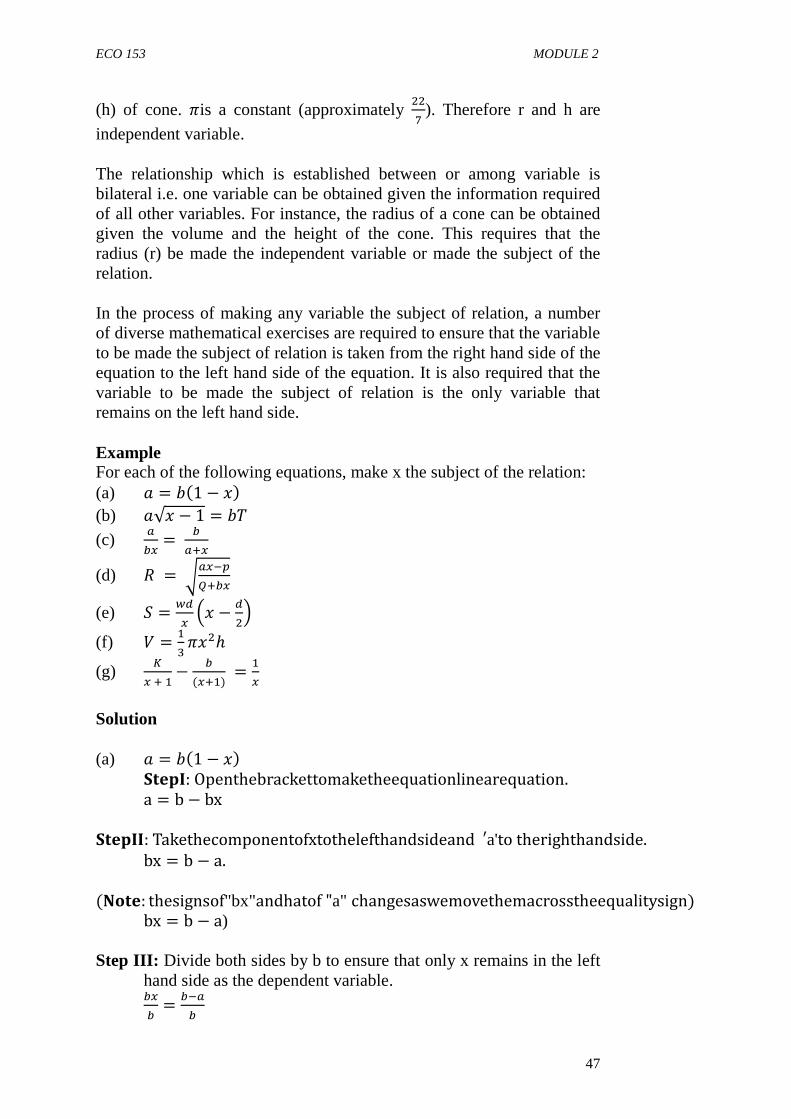
ECO 153 MODULE 2
47
(h) of cone. �is a constant (approximately �� ). Therefore r and h are
independent variable. The relationship which is established between or among variable is bilateral i.e. one variable can be obtained given the information required of all other variables. For instance, the radius of a cone can be obtained given the volume and the height of the cone. This requires that the radius (r) be made the independent variable or made the subject of the relation.
In the process of making any variable the subject of relation, a number of diverse mathematical exercises are required to ensure that the variable to be made the subject of relation is taken from the right hand side of the equation to the left hand side of the equation. It is also required that the variable to be made the subject of relation is the only variable that remains on the left hand side. Example For each of the following equations, make x the subject of the relation: (a) � = ��1 − � (b) �√� − 1 = �
(c) �� = ���
(d) � = � ����� (e) � = ��
� �� − ���
(f) � = �����ℎ
(g) ����−
�(���) = �
� Solution (a) � = ��1 − � �����:Openthebrackettomaketheequationlinearequation. a = b − bx ������:Takethecomponentofxtothelefthandsideand a� 'totherighthandside. bx = b − a. (����: thesignsof"bx"andhatof"a" changesaswemovethemacrosstheequalitysign) bx = b − a) Step III: Divide both sides by b to ensure that only x remains in the left hand side as the dependent variable.
��� = �
�
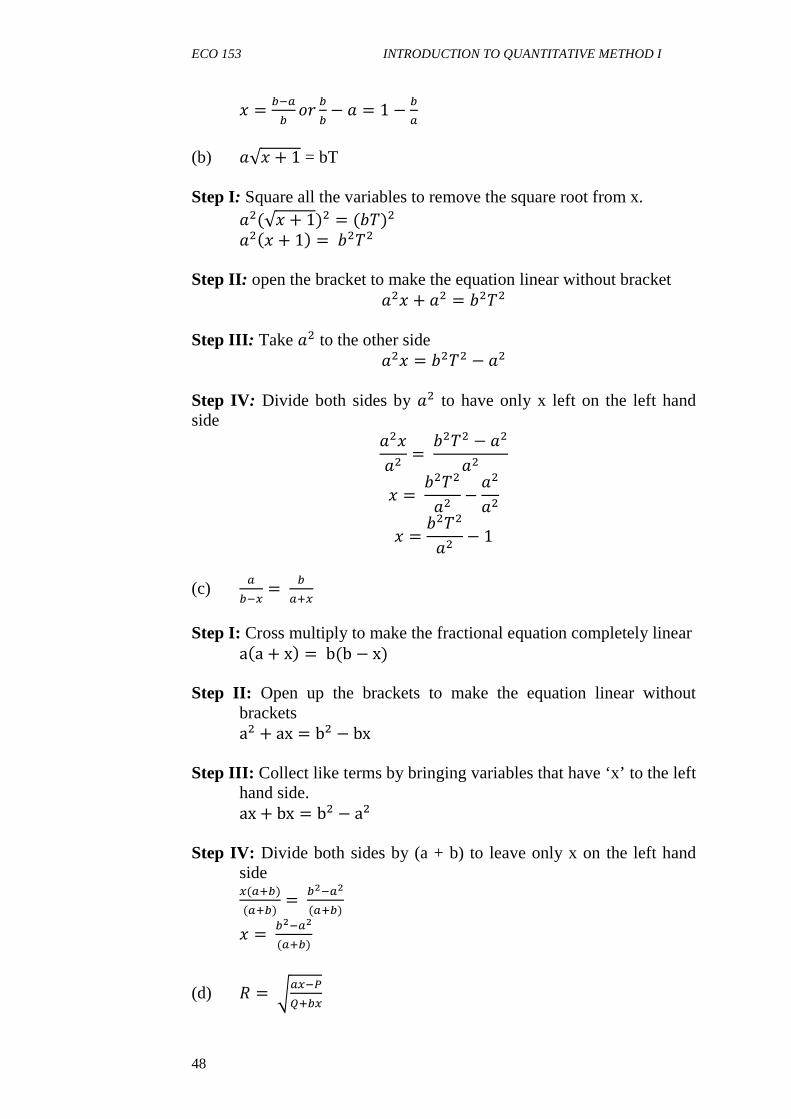
ECO 153 INTRODUCTION TO QUANTITATIVE METHOD I
48
� = � � �� �� − � = 1 − �
(b) �√� + 1 = bT Step I: Square all the variables to remove the square root from x. ��(√� + 1)� = (�)� ���� + 1 = ��� Step II: open the bracket to make the equation linear without bracket ��� + �� = ��� Step III: Take �� to the other side ��� = ��� − �� Step IV: Divide both sides by �� to have only x left on the left hand side ����� = ��� − ����
� = ����� − ���� � = ����� − 1
(c) � � = ���
Step I: Cross multiply to make the fractional equation completely linear a�a + x = b(b − x) Step II: Open up the brackets to make the equation linear without brackets a� + ax = b� − bx Step III: Collect like terms by bringing variables that have ‘x’ to the left hand side. ax + bx = b� − a� Step IV: Divide both sides by (a + b) to leave only x on the left hand side
�(��)(��) = �� �(��)
� = �� �(��)
(d) � = � �����
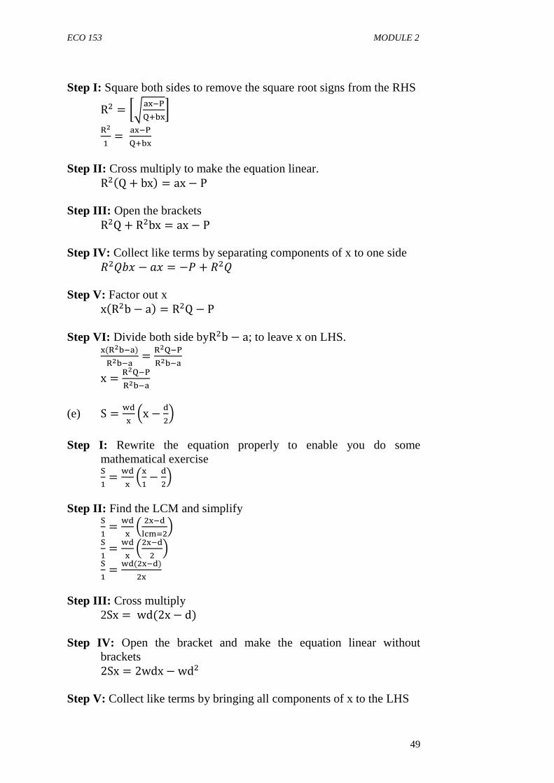
ECO 153 MODULE 2
49
Step I: Square both sides to remove the square root signs from the RHS
R� = � �� ������
��� = �� �����
Step II: Cross multiply to make the equation linear. R��Q + bx = ax − P Step III: Open the brackets R�Q + R�bx = ax − P Step IV: Collect like terms by separating components of x to one side ����� − �� = −� + ��� Step V: Factor out x x�R�b − a = R�Q − P Step VI: Divide both side byR�b − a; to leave x on LHS.
�(��� �)��� � = ��� �
��� � x = ��� �
��� �
(e) S = ��� �x − �
��
Step I: Rewrite the equation properly to enable you do some mathematical exercise
�� =
��� ���− �
��
Step II: Find the LCM and simplify
�� =
��� � �� ��� !��
�� =
��� ��� �� �
�� =
��(�� �)��
Step III: Cross multiply 2Sx = wd(2x − d) Step IV: Open the bracket and make the equation linear without brackets 2Sx = 2wdx − wd� Step V: Collect like terms by bringing all components of x to the LHS
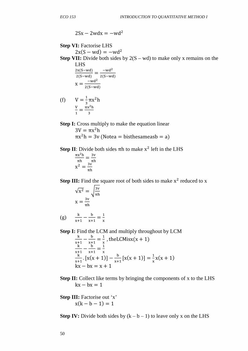
ECO 153 INTRODUCTION TO QUANTITATIVE METHOD I
50
2Sx − 2wdx = −wd� Step VI: Factorise LHS 2x�S − wd = −wd� Step VII: Divide both sides by 2(S – wd) to make only x remains on the LHS
��(� ��)�(� ��) = ���
�(� ��) x = ���
�(� ��)
(f) V = ��πx�h
"� =
#��$�
Step I: Cross multiply to make the equation linear 3V = πx�h πx�h = 3v(Notea = bisthesameasb = a) Step II: Divide both sides πh to make x� left in the LHS
#��$#$ = �%
#$ x� = �%
#$ Step III: Find the square root of both sides to make x� reduced to x
√x� = �%#$ x = �%
#$
(g) &���−
���� =
��
Step I: Find the LCM and multiply throughout by LCM
&���−
���� =
�� , theLCMisx(x + 1)
&���−
���� =
��
&��� . [x�x + 1] − �
��� [x�x + 1] = �� x�x + 1
kx − bx = x + 1 Step II: Collect like terms by bringing the components of x to the LHS kx − bx = 1 Step III: Factorise out ‘x’ x�k − b − 1 = 1 Step IV: Divide both sides by (k – b – 1) to leave only x on the LHS
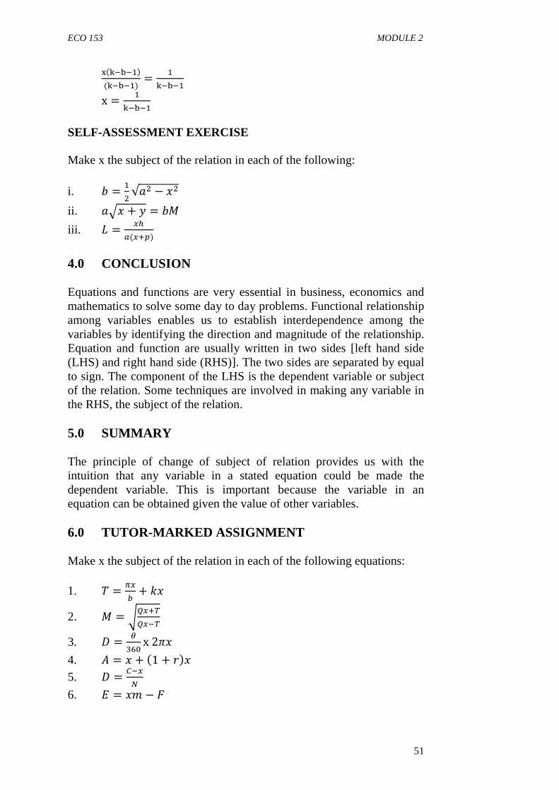
ECO 153 MODULE 2
51
�'& � �((& � �) = �
& � � x = �
& � �
SELF-ASSESSMENT EXERCISE
Make x the subject of the relation in each of the following:
i. � = ��√�� − ��
ii. ��� + � = ��
iii. = �)(���)
4.0 CONCLUSION
Equations and functions are very essential in business, economics and mathematics to solve some day to day problems. Functional relationship among variables enables us to establish interdependence among the variables by identifying the direction and magnitude of the relationship. Equation and function are usually written in two sides [left hand side (LHS) and right hand side (RHS)]. The two sides are separated by equal to sign. The component of the LHS is the dependent variable or subject of the relation. Some techniques are involved in making any variable in the RHS, the subject of the relation.
5.0 SUMMARY
The principle of change of subject of relation provides us with the intuition that any variable in a stated equation could be made the dependent variable. This is important because the variable in an equation can be obtained given the value of other variables.
6.0 TUTOR-MARKED ASSIGNMENT
Make x the subject of the relation in each of the following equations: 1. = *�
� + !�
2. � = ������ � 3. " = +
�,� x2��
4. # = � + �1 + ��
5. " = - �.
6. $ = �% − &

ECO 153 INTRODUCTION TO QUANTITATIVE METHOD I
52
7. �� +
�/ =
�0
7.0 REFERENCES/FURTHER READING Channon, et al. (1990).New General Mathematics for West Africa. (4th
ed.). United Kingdom:Longman Group. Usman, A. S. (2005). Business Mathematics. Lagos: Apex Books
Limited.
ECO 153 MODULE 2
53
UNIT 2 LINEAR EQUATIONS AND LINEAR SIMULTANEOUSEQUATION CONTENTS 1.0 Introduction 2.0 Objectives 3.0 Main Content 3.1 General Overview 3.2 Solving Linear Equation 3.3 Simultaneous Linear Equation 3.4 Linear Equation using Gradient of a Straight Line 4.0 Conclusion 5.0 Summary 6.0 Tutor-Marked Assignment 7.0 References/Further Reading 1.0 INTRODUCTION
A linear equation is the simplest form of equation. It is an equation that has a highest power of 1 and when graphed on a plane scale, it produces a straight line graph. A typical linear equation has the form of y = mx + c, where:
y = dependent variable m = slope of the graph c = intercept of the graph x = independent variable.
Most often than none, because of its simplicity, linear equations are used in economics and business to establish functional relationship among variables. Examples include relationship between quantity demanded and price e.g. Qd = 40 – 3p relationship between consumption and disposable income e.g. C = 40 + 0.6Yd, etc.
2.0 OBJECTIVES
At the end of this unit, you should be able to: • explain the components of a linear equation • solve linear equations • solve simultaneous linear equations.
ECO 153 INTRODUCTION TO QUANTITATIVE METHOD I
54
3.0 MAIN CONTENT 3.1 General Overview
Most relationship in economics and business are expressed in single linear terms, not only for simplicity purpose but also for easy assignment in terms of the magnitude and direction of the variables concerned. A linear equation is a mathematical statement which shows that two algebraic terms or expressions are equal. The algebraic terms should have the highest power of terms equal to 1. For example:
(a) 2� + 9 = 27 (b) � + 4 = 5 − 3� (c) 9 = 4 − 2' (d) 2� + 2� = 1
In examples a, b and c above, the unknown in each of the equations is x. x has the highest power of 1 in each case. In example (d), we have a linear equation with two unknowns. In equation (a), (b) and (c), the unknown can easily be obtained by collecting like terms and dividing by the coefficient of the unknown. In the case of example (d), there are two unknowns in a single linear equation. The value unknowns cannot be obtained in (d) unless another similar equation is provided, thereby, making the two equations a pair of simultaneous linear equation.
SELF-ASSESSMENT EXERCISE
i. Explain the term “linear equation”? How is it different from other
forms of equations? ii. Why is linear equations commonly used in establishing
relationship between or among variables? 3.2 Solving Linear Equation
In solving a linear equation to obtain the value of the unknown – three major steps are required: a) collect like terms b) add/subtract the like terms to/from the one another c) divide throughout by the coefficient of the unknown. Example: Solve for the unknown in each of the following equations: i. 20 − 3� = 17 ii. 20 − 8� = 2 + � iii. 25 − 5� = 5� iv. 6� + 9 = 63 − 3� v. 2� + 19 − 5� = � − 5

ECO 153 MODULE 2
55
Solution i. 20 + 3� =17 Collecting like terms
20 − 17 = 3� 3 = 3���3� = 3
Divide through by 3 (the co-efficient of y)
�/� = �
� � = 1 Note: To confirm the correctness of the value obtained, you can substitute the value back to the equation and see whether the LHS equals the RHS. If it does not, then the solution obtained is wrong. For example:
20 − 3� = 17 Substituting y = 1 20 − 3�1 = 17 20 − 3 = 17 17 = 17.Hence, y = 1isabsolutelycorrect.
ii. 20 − 8� = 2 + � Collecting like terms
20 − 2 = � + 8� 18 = 9�
Divide both sides by 9
1�1 = �2
1 � = 2. iii. 25 − 5� = 5� Collecting like terms,
25 = 5� + 5� 25 = 10���10� = 25 Dividing both sides by 10
����� = �3
�� � = �3
�� =3� ��2 ��.
iv. 6� + 9 = 63 − 3� Collecting like terms 6� + 3� = 63 − 9 9� = 54 Divide both sides by 9
1�1 = 34
1
� = 6
ECO 153 INTRODUCTION TO QUANTITATIVE METHOD I
56
v. 2� + 19 − 5� = � − 5 Collect like terms 2� − 5� − � = 15 − 19 −4� = 24 Divide both sides by -4
4� 4 = �4 4
� = 6 SELF-ASSESSMENT EXERCISE i. Solve for x in each of the following equations:
(a) 42 = 7� − 14 (b) 18 − 2� = 4� − 12 (c) 5� + 17 = 2� + 41 (d) 2� + 5 = 13 (e) 2�2� + 9 = 3(4� − 10)
ii. Given that the quantity demand of orange �( = 40 − 5�
(a) What quantity of orange is demanded if price is N5? (b) At what price will 25 units of oranges demanded?
iii. Given the quantity demand and quantity supplied as�) = −20 +
3��*(�( = 220 − 5�. Determine the equilibrium price for the market (Hint: equate Qs and Qd and solve for P i.e. −20 + 3� =220 − 5�.
3.3 Simultaneous Linear Equation A simultaneous linear equation is a set of linear equations in which the numbers of the equations equal the number of unknown. The two commonest mathematical approaches of solving simultaneous equation are:
i. Elimination method ii. Substitution method
Elimination Method: This involves multiplying the coefficient of the unknown by some constant values so as to make one of the unknowns have the same coefficient and therefore eliminated leaving only one unknown that could be solved using simple linear equation technique. Example 1
2� + 5� = 2 � − 2� = 10 Solution 2� + 5� = 2……………. x 1
ECO 153 MODULE 2
57
� − 2� = 10 …………….. x 2 –2� + 5� = 2 2� − 4� = 20 5� − �−4� = 2 − 20 5� + 4� = −18 9� = −18 Divide both sides by 9 9�9 = −18
9 � = −2 From equation (ii) � − 2� = 10 � − 2�−2 = 10 � + 4 = 10 � = 10 − 4 = 6
Example 2 � + � − + = 0 ……………………. (i)
3� − 2� = 4+ = 11 ……………… (ii) 5� − � − + = 0 …………………... (iii) From (i) and (ii) � + � − + = 0 ……………………. x 3 3� − 2� = 4+ = 11 ……………… x 1 –3� + 3� − 3+ = 0
3� − 2� = 4+ = 11 3� − �−2� − 3+ − �4+ = 0 − 11 5� − 7+ = −11…………………….. (iv) From (ii) and (iii) 3� − 2� = 4+ = 11 ……………… x 5 5� − � − + = 0 …………………... x 3 –15� − 10� + 20+ = 55
15� − 3� − 3+ = 0 −10� − �+3�+ 20+ − �−3+ = 55 − 0 10� − 3� + 20+ + 3+ = 55 7� + 23+ = 55 …………………… (v) Solving (iv) and (v) simultaneously 5� − 7+ = −11 ………………… x -7 −7� + 23+ = 55 ………………… x 5 –−35� + 49+ = 77
ECO 153 INTRODUCTION TO QUANTITATIVE METHOD I
58
−35� + 115+ = 275 49+ − 115+ = 77 − 275 −66+ = −198 + = −198
−66 = 3.
From equation (iv) 5� − 7+ = −11 5� − 7�3 = −11 5� − 21 = −11 5� = −11 + 21 5� = 10 � = ��
3 = 2
From equation (i) � + � − + = 0
� + 2 − 3 = 0 � − 1 = 0 � = 1
Substitution Method: Substitution method requires writing one of the unknown of the equation in terms of the unknown. The equation obtained is therefore substituted to the other equation.
e.g.2� − 4� = −4 ………………… (i) 3� + 2� = 18 ………………… (ii)
From equation (i) 2� = −4 + 4�
� = 4�4/� ……………….. (iii)
Substitute equation (iii) into equation (ii)
3 , 4�4/� -+ 2� = 18 −12 + 12�
2 + 2�1 = 18
1
Multiply through by 2 −12 + 12� + 4� = 36
12� + 4� = 36 + 12 16� = 48 � = 48
16 = 3
From equation (i) 2� − 4� = −4 2� − 4�3 = −4 2� − 12 = −4 2� = −4 + 12 2� = 8 � = 8
2 � = 4

ECO 153 MODULE 2
59
SELF-ASSESSMENT EXERCISE i. Solve the following pairs of simultaneous equation using
elimination method: (a) 2x – y = 8 3x + y =17 (b) a – b + c = 2 2a – 2b + c =3 4a – 3b + 2c = 7
ii. Use substituting method to solve for p and q if:
2p – 3q = 1 3p + 2q = 21
iii. The equilibrium conditions of two markets, butter and margarine, where Pb and Pm are the prices of butter and margarine respectively, are given as:
8Pb – 3Pm = 7 and –Pb + 7Pm = 19. Find the prices of butter and margarine.
4.0 CONCLUSION Linear equation may have one unknown or more than one unknown. When a linear equation has only one unknown, it is a simple linear equation and it can be solved by collecting like terms and dividing by the coefficient of the unknown after simplification. When it has more than one unknowns, for instance, two equations of the same type and number of unknown for the unknowns to be solved. Any of the two techniques of solving simultaneous equation (elimination or substitution method) could be used to solve a pair of a simultaneous linear equation. 5.0 SUMMARY
The procedures for solving simple linear equation and simultaneous linear equation should be able to produce answer(s) such that when substituted back to the equation, give the same answer at both the right hand side and left hand side of the equation. This is a quick way of testing for the correctness of the answer(s) obtained. 6.0 TUTOR-MARKED ASSIGNMENT 1. Solve for x in each of the following equation:
a) 10� + 60 = 10 + 5�3 − � b) 3�2� − 5 = 9 c) 21 − �6� + 7 = 8�3 − 2� d) 43 − 3�7 − � = 4 − 3�

ECO 153 INTRODUCTION TO QUANTITATIVE METHOD I
60
2. Solve for x and y in each of the following equation: i. 3� + 4� = 12
9� + 2� = −9
ii. 2� − 3� = 10 � − 3� = 8
iii. 3� + � = 10 3� − 2� = −2
iv. 2� − 3� = 6 � − 2� = 5 3. 8 Choco and 3 pens cost N288 while 5 Choco and 2 pens cost
N184, (a) Find the cost of a Choco (b) Find the cost of a pen.
[Hint: let Choco be x and pen be y i.e. equation 1 is 8x + 3y = 288] 7.0 REFERENCES/FURTHER READING Murray, L. (1987). Progress in Mathematics. Stanley Thornes
Publishers. Usman, A. S. (2005). Business Mathematics. Lagos: Apex Books
Limited.

ECO 153 MODULE 2
61
UNIT 3 QUADRATIC EQUATION CONTENTS 1.0 Introduction 2.0 Objectives 3.0 Main Content 3.1 General Overview 3.2 Factorisation 3.3 Completing the Square Method 3.4 Formula Method 3.5 Perfect Square 4.0 Conclusion 5.0 Summary 6.0 Tutor-Marked Assignment 7.0 References/Further Reading 1.0 INTRODUCTION In Unit 2 of this module, we defined a linear equation as an equation which has its highest power as 1 e.g. 3x + 12, 3x =16, etc. it is possible for an equation to have its highest power as 2 such as x2 – 4x + 5 =0, x2 = 25, x2 + x =5 etc. These are called quadratic equations. It is an equation as a result of the equal sign, if it is written without equal to sign, such as x2 + 4x – 5, x2 – 16, x2 –x, it is called quadratic expression. 2.0 OBJECTIVES At the end of this unit, you should be able to: • identify quadratic equation and expression • factorise quadratic expressions • solve for the unknown in a quadratic equation • identify perfect squares and make equations perfect squares. 3.0 MAIN CONTENT 3.1 General Overview Quadratic equations can be solved using different approaches or methods. Common among these methods are factorisation, completing the square, formula method and the graphical method. Recall that, in solving a linear equation, a single answer is obtained. In solving a quadratic equation, two different answers are obtained. The general
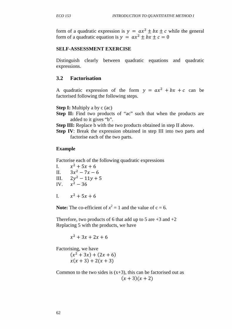
ECO 153 INTRODUCTION TO QUANTITATIVE METHOD I
62
form of a quadratic expression is � = ��� ± �� ± + while the general form of a quadratic equation is � = ��� ± �� ± + = 0 SELF-ASSESSMENT EXERCISE Distinguish clearly between quadratic equations and quadratic expressions. 3.2 Factorisation
A quadratic expression of the form � = ��� + ��+ + can be factorised following the following steps. Step I: Multiply a by c (ac) Step II: Find two products of “ac” such that when the products are
added to it gives “b”. Step III: Replace b with the two products obtained in step II above. Step IV: Break the expression obtained in step III into two parts and
factorise each of the two parts. Example Factorise each of the following quadratic expressions I. �� + 5� + 6 II. 3�� − 7� − 6 III. 2�� − 11� + 5 IV. �� − 36 I. �� + 5� + 6
Note: The co-efficient of x2 = 1 and the value of c = 6. Therefore, two products of 6 that add up to 5 are +3 and +2 Replacing 5 with the products, we have �� + 3� + 2� + 6 Factorising, we have ��� + 3�+ �2� + 6 ��� + 3+ 2(� + 3) Common to the two sides is (x+3), this can be factorised out as �� + 3(� + 2)
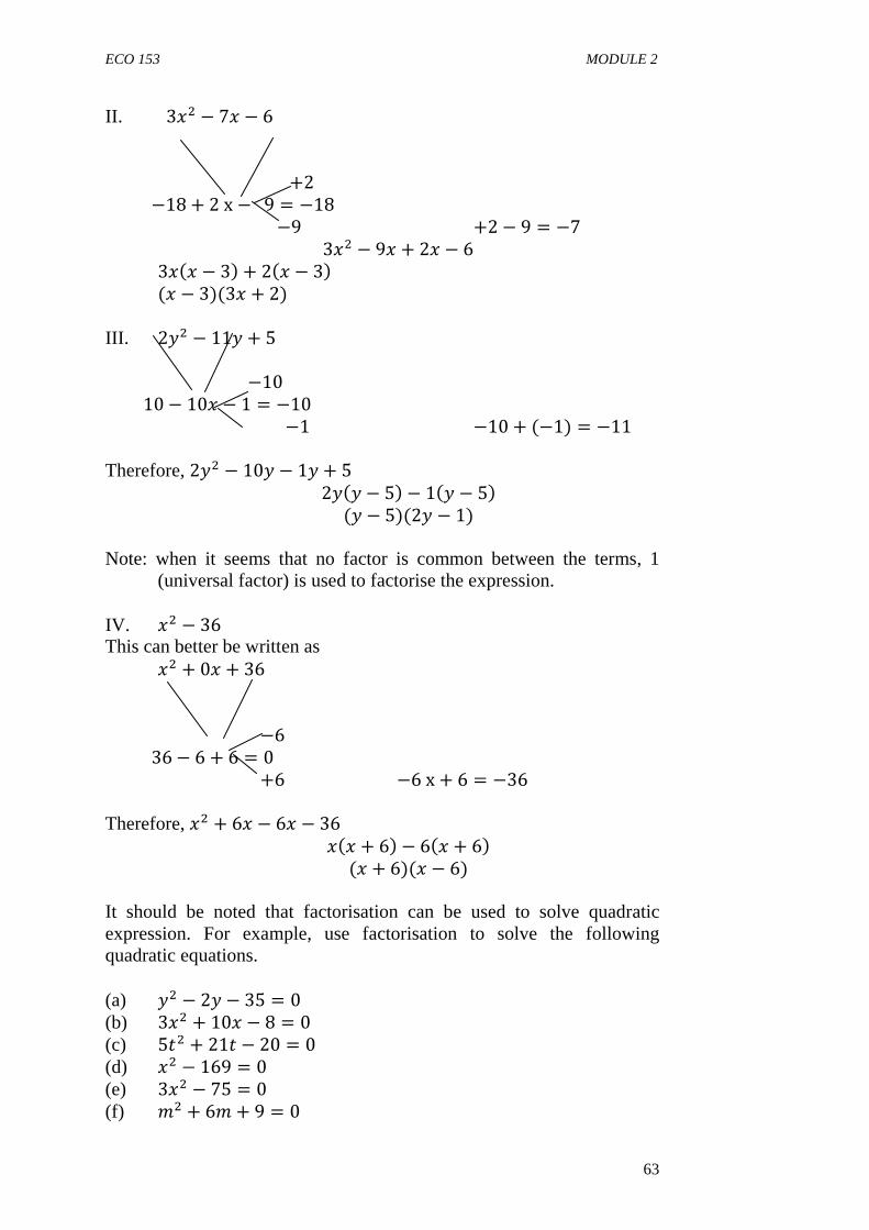
ECO 153 MODULE 2
63
II. 3�� − 7� − 6 +2 −18 + 2x − 9 = −18 −9 +2 − 9 = −7
3�� − 9� + 2� − 6 3��� − 3+ 2�� − 3 (� − 3)(3� + 2)
III. 2�� − 11� + 5 −10 10 − 10� − 1 = −10 −1 −10 + (−1) = −11 Therefore, 2�� − 10� − 1� + 5
2��� − 5− 1�� − 5 (� − 5)(2� − 1)
Note: when it seems that no factor is common between the terms, 1
(universal factor) is used to factorise the expression. IV. �� − 36 This can better be written as �� + 0� + 36 −6 36 − 6 + 6 = 0 +6 −6x + 6 = −36 Therefore, �� + 6� − 6� − 36 ��� + 6− 6�� + 6
(� + 6)(� − 6) It should be noted that factorisation can be used to solve quadratic expression. For example, use factorisation to solve the following quadratic equations. (a) �� − 2� − 35 = 0 (b) 3�� + 10� − 8 = 0 (c) 5.� + 21. − 20 = 0 (d) �� − 169 = 0 (e) 3�� − 75 = 0 (f) %� + 6% + 9 = 0
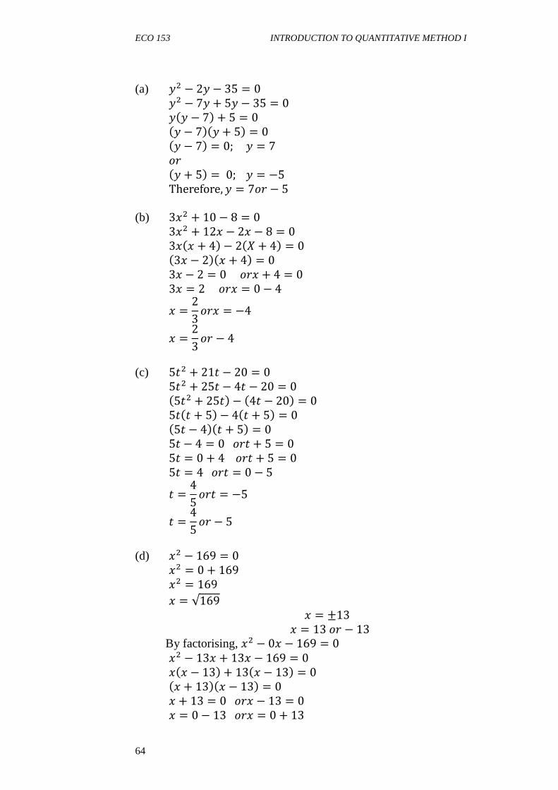
ECO 153 INTRODUCTION TO QUANTITATIVE METHOD I
64
(a) �� − 2� − 35 = 0 �� − 7� + 5� − 35 = 0 ��� − 7+ 5 = 0 �� − 7�� + 5 = 0 �� − 7 = 0; � = 7 �� �� + 5 = 0; � = −5
Therefore,� = 7�� − 5 (b) 3�� + 10 − 8 = 0
3�� + 12� − 2� − 8 = 0 3��� + 4− 2�/ + 4 = 0 �3� − 2�� + 4 = 0 3� − 2 = 0��� + 4 = 0 3� = 2��� = 0 − 4 � = 2
3 ��� = −4 � = 23 �� − 4
(c) 5.� + 21. − 20 = 0
5.� + 25. − 4. − 20 = 0 �5.� + 25.− �4. − 20 = 0 5.�. + 5− 4�. + 5 = 0 �5. − 4�. + 5 = 0 5. − 4 = 0��. + 5 = 0 5. = 0 + 4��. + 5 = 0 5. = 4��. = 0 − 5 . = 4
5 ��. = −5 . = 45 �� − 5
(d) �� − 169 = 0 �� = 0 + 169 �� = 169 � = √169 � = ±13 � = 13�� − 13 By factorising, �� − 0� − 169 = 0 �� − 13� + 13� − 169 = 0 ��� − 13+ 13�� − 13 = 0 �� + 13�� − 13 = 0 � + 13 = 0��� − 13 = 0 � = 0 − 13��� = 0 + 13
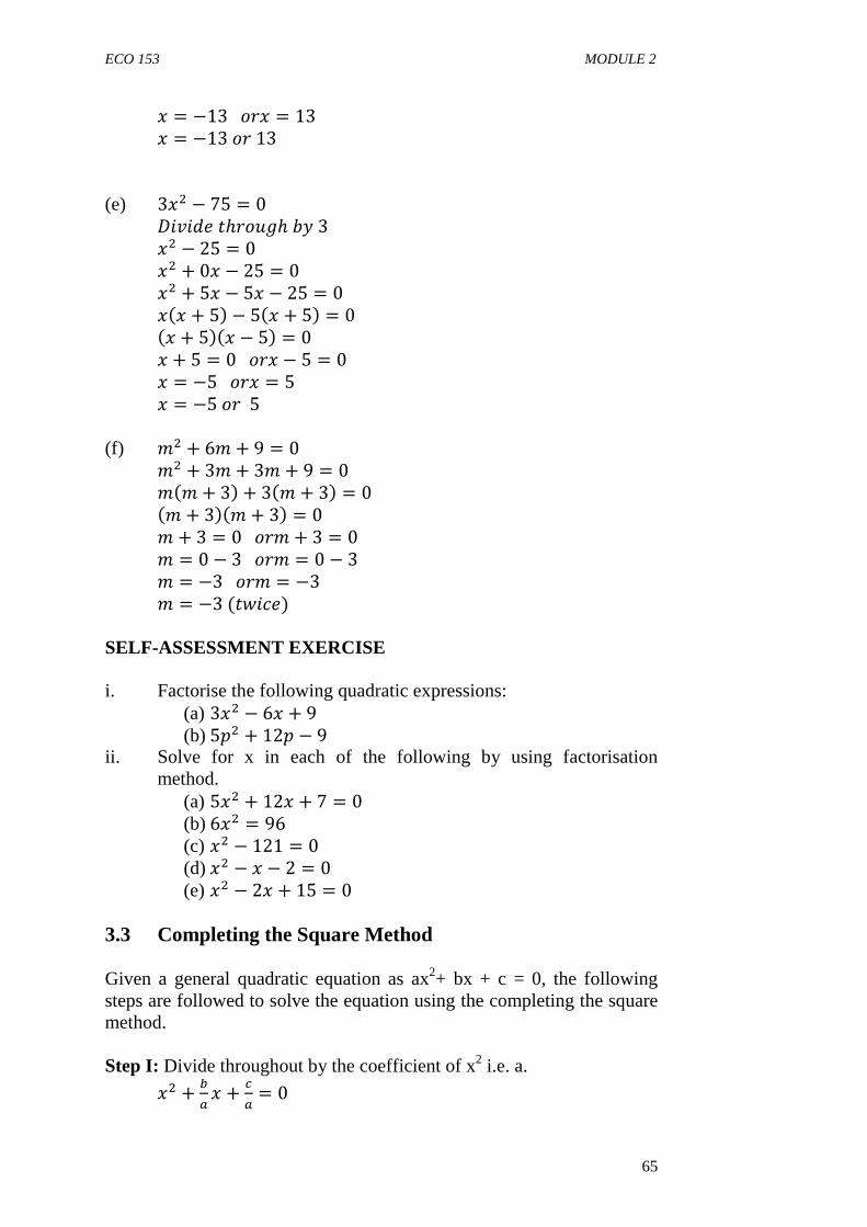
ECO 153 MODULE 2
65
� = −13��� = 13 � = −13��13 (e) 3�� − 75 = 0 "010(2.ℎ��34ℎ��3 �� − 25 = 0 �� + 0� − 25 = 0 �� + 5� − 5� − 25 = 0 ��� + 5− 5�� + 5 = 0 �� + 5�� − 5 = 0 � + 5 = 0��� − 5 = 0 � = −5��� = 5 � = −5��5 (f) %� + 6% + 9 = 0 %� + 3% + 3% + 9 = 0 %�% + 3+ 3�% + 3 = 0 �% + 3�% + 3 = 0 % + 3 = 0��% + 3 = 0 % = 0 − 3��% = 0 − 3 % = −3��% = −3 % = −3(.50+2) SELF-ASSESSMENT EXERCISE
i. Factorise the following quadratic expressions:
(a) 3�� − 6� + 9 (b) 56� + 126 − 9
ii. Solve for x in each of the following by using factorisation method.
(a) 5�� + 12� + 7 = 0 (b) 6�� = 96 (c) �� − 121 = 0 (d) �� − � − 2 = 0 (e) �� − 2� + 15 = 0
3.3 Completing the Square Method
Given a general quadratic equation as ax2+ bx + c = 0, the following steps are followed to solve the equation using the completing the square method. Step I: Divide throughout by the coefficient of x2 i.e. a.
�� + � � + 5
= 0
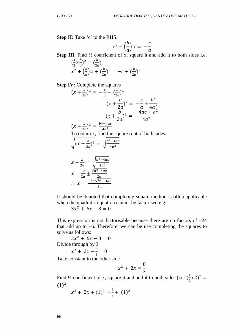
ECO 153 INTRODUCTION TO QUANTITATIVE METHOD I
66
Step II: Take ‘c’ to the RHS. �� + 7��8 � = − +�
Step III: Find ½ coefficient of x, square it and add it to both sides i.e.
(�� x�)� = ( ��)
�� + ��� � + ( ��)� = −+ + ( ��)� Step IV: Complete the squares
(� + ��)� = − 5
+ ( ��)� (� + �
2�)� = − +� + ��4��
(� + �2�)� = −4�+ + ��
4��
(� + ��)� = �� 454�
To obtain x, find the square root of both sides
(� + ��)� = �� 454�
� + �� = �� 454�
� = �� ±
√�� 45�
... � = �±√�� 45�
It should be denoted that completing square method is often applicable when the quadratic equation cannot be factorised e.g. 3�� + 6� − 8 = 0 This expression is not factorisable because there are no factors of –24 that add up to +6. Therefore, we can be use completing the squares to solve as follows: 3�� + 6� − 8 = 0 Divide through by 3.
�� + 2� − 2� = 0
Take constant to the other side �� + 2� = 83
Find ½ coefficient of x, square it and add it to both sides (i.e. (�� �2)� =(1)� �� + 2� + (1)� = 2
� + (1)�
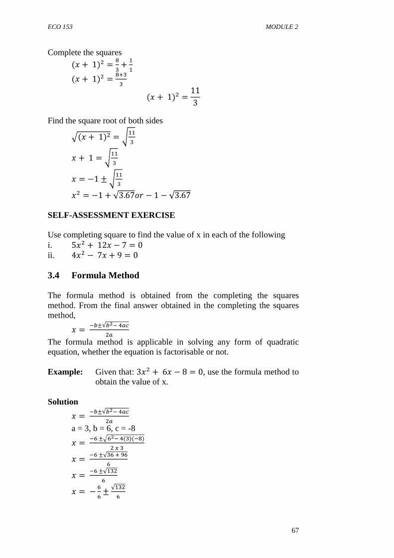
ECO 153 MODULE 2
67
Complete the squares
(� + 1)� = 2�+
��
(� + 1)� = 2���
(� + 1)� = 113
Find the square root of both sides
�(� + 1)� = ���
� + 1 = ���
� = −1 ± ���
�� = −1 + √3.67�� − 1 − √3.67 SELF-ASSESSMENT EXERCISE Use completing square to find the value of x in each of the following i. 5�� + 12� − 7 = 0 ii. 4�� − 7� + 9 = 0 3.4 Formula Method The formula method is obtained from the completing the squares method. From the final answer obtained in the completing the squares method,
� = �±√�� 45�
The formula method is applicable in solving any form of quadratic equation, whether the equation is factorisable or not. Example: Given that: 3�� + 6� − 8 = 0, use the formula method to
obtain the value of x.
Solution
� = �±√�� 45�
a = 3, b = 6, c = -8
� = ,±7,� 4(�)( 2)���
� = ,±√�,�1,,
� = ,±√���,
� = − ,,± √���,

ECO 153 INTRODUCTION TO QUANTITATIVE METHOD I
68
� = − ,,± √���,
� = −1± √4���,
� = −1± �√��,
� = −1± √���
� = −1 − √��� �� − 1 + √���
Note:�� − 4�+ is called Discriminant (D), if D = 0 or �� = 4�+ - the quadratic equation has two equal answers.
If �� > 4�+ or D > 0, we have two distinct answers; and If �� < 4�+ or D < 0, we have complex number as answers.
SELF-ASSESSMENT EXERCISE
Use formula method to solve the unknown in each of the following equations. i. 5�� − 12� − 9 = 0 ii. 3%� − 4% + 2 = 0 3.5 Perfect Square
A perfect square is a quadratic expression that has the same term after factorisation. A quadratic equation is said to be perfect square when it has two equal answers or roots. This implies that; �� − 4�+ =0���� = 4�+
Examples include: �� + 4� + 4 = 0 �� + 2� + 2� + 4 ��� + 2+ 2�� + 2
(� + 2)(� + 2) Example 1: Find the value of K for which each of the following to be a perfect square:
(a) 12�� − 6� + 9 (b) 2�� + 8� + 9
Example 2: Find the quadratic equation whose roots are: (a) -1 and 4 (b) 3 and 2 (c) -3 twice
Solution
(a) 12�� − 6� + 9

ECO 153 MODULE 2
69
�� = 4�+ (−6)� = 4�129
36 = 489 9 = 3648 = 3
4
... 12�� − 6� + �4 0)�62�:2+.)'3��2. 48�� − 24� + 3is a perfect square ;ℎ2+!: 48�� − 12� − 12� + 3
= 12��4� − 1− 3(4� − 1) = �4� − 1(12� − 3) = �4� − 1�4� − 1<�.2: 12� − 3 = 4� − 1
(b) 2�� + 8� + 9 �� = 4�+ (8)� = 4�29 64 = 89 9 = ,4
2 = 8
Therefore, 2�� + 8� + 8 = 0 is a perfect square. Check: 2�� + 4� + 4� + 8 2��� + 2+ 4�� + 2 �2� + 4�� + 2 (� + 2)(� + 2) Example 2
(a) �� + 1�� − 4 = 0Note: there is a change in the signs of the roots. ��� + 1− 4�� + 1 = 0 �� + � − 4� − 4 = 0 �� − 3� − 4 = 0
(b) �� − 3�� − 2 = 0 ��� − 2− 3�� − 2 = 0 �� − 2� − 3� + 6 = 0 �� − 5� + 6 = 0 (c) �� + 3�� + 3 = 0 ��� + 3+ �� + 3 = 0 �� + 3� + 3� + 9 = 0 �� + 6� + 9 = 0

ECO 153 INTRODUCTION TO QUANTITATIVE METHOD I
70
SELF-ASSESSMENT EXERCISE i. Find the value of K for each of the following to be a perfect
square. (a) 4�� − 8� + 9 (b) �� + 4� + 9
ii. Check whether each of the following equations is perfect squares or not. (Hint: use b2 = 4ac) (a) 3�� − 12� + 6 (b) 2�� + 8� + 8 (c) 2�� − 8� + 16
iii. Find the quadratic equation whose roots are:
(i) − ���*( �� (ii) 4�*( − 3 (iii) 2 twice
4.0 CONCLUSION Quadratic equation can be simply solved using factorisation method. When the equation is not factorisable, completing the square method or formula method is used. 5.0 SUMMARY Quadratic equations are non-linear equation in which the highest power of the terms is 2. When quadratic expressions are factorised, two distinct or different terms are obtained. Likewise when a quadratic equation is solved, two different or distinct answers are obtained depending on the value of the Discriminant (D). When the roots or answer are the same, the expression or equation becomes a perfect square. 6.0 TUTOR-MARKED ASSIGNMENT 1. Factorise the following quadratic expressions: (a) 6� − 56' − 6'� (b) 4.� − 12. + 5 2. Solve for x in each of the following using factorisation method. (a) 3�� − 23� − 8 = 0 (b) �� − 8� − 9 = 0 3. The following equations are not factorisable, use any method of
your choice to solve for x: (i) 3�� + 9� − 8 = 0
(ii) 5�� + 14� + 6 = 0
ECO 153 MODULE 2
71
4. Find the quadratic equation whose roots are: (a) -4 twice (b) -1 and ½ (c) +3 and -6
5. Find the value of K required to make each of the following a perfect square. (i) 4�� − 12� + 9 (ii) 5�� − 14� + 9 (iii) 3�� + 6� + 9
7.0 REFERENCES/FURTHER READING
Channon, et al. (2003).New General Mathematics for Senior Secondary
Schools Book 1&2. United Kingdom: Longman Publishing Company.
Edward, T. D. (2001). Introduction to Mathematical Economics. (3rd
ed.). Tata McGraw-Hill.
ECO 153 INTRODUCTION TO QUANTITATIVE METHOD I
72
UNIT 4 SIMULTANEOUS LINEAR AND QUADRATIC EQUATIONS CONTENTS 1.0 Introduction 2.0 Objectives 3.0 Main Content 3.1 General Overview 3.2 Simultaneous Linear and Quadratic Equations 4.0 Conclusion 5.0 Summary 6.0 Tutor-Marked Assignment 7.0 References/Further Reading 1.0 INTRODUCTION In Units two and three of this module, we discussed linear equations linear simultaneous equation and quadratic equations. We discussed the approaches of solving two linear simultaneous equations (substitution and elimination method). Sometimes, there could be simultaneous equation comprising of two equations; one linear and the other quadratic. These equations are solved simultaneously by using a combination of substitution method and factorisation techniques. Examples of such pairs of simultaneous equation are: �� + �� = 70; � + � = 8 � + � = 7; �� + 2�� − 3 = � It should be noted that, in each of the examples cited above, at least two values are obtained for each of the unknowns (x and y). 2.0 OBJECTIVE At the end of this unit, you should be able to: • solve pairs of simultaneous linear equation and quadratic
equations.
ECO 153 MODULE 2
73
3.0 MAIN CONTENT 3.1 General Overview Linear equations and quadratic equations have different traits or characteristics. Yet, they could be solved simultaneously. The tendency of the quadratic component to give two roots or two answers will generate two answers/roots to each of the unknown except in few cases of repeated roots. In most cases, we factorise the quadratic equation to obtain the roots of the equation which are substituted to the other equation. In some cases, we write one of the unknowns in a linear equation and substitute it into the quadratic equation. Whichever the approach employed, multiple values of each of the unknowns are most likely to be the result. SELF-ASSESSMENT EXERCISE Explain how a linear and a quadratic equation could be solved simultaneously. 3.2 Simultaneous Linear and Quadratic Equation Solve for x and y if:
(a) � − � = 4 4�� + 5� − 51 = 0
(b) � + � = 10 �� = 21 (c) 2� − � = 6 �� + �� = 41
Solution
(a) � − � = 4 …………………………… (i) 4�� + 5� − 51 = 0 ………………….. (ii) From (ii), 4�� + 5� − 51 = 0 4�� + 17� − 12� − 51 = 0 ��4� + 17− 3�4� + 17 = 0 �� − 3�4� + 17 = 0 � − 3 = 0; � = 3 ��4� + 17 = 0; 4� = −17; � = −17
4
From equation (i), � − � = 4 � = 4 + � =:� = 3,� = 4 + 3 = 7 =:� = −17
3 ,� = 4 + 7−173 8
ECO 153 INTRODUCTION TO QUANTITATIVE METHOD I
74
= 4 − 5 �� = −1 �� �� − 3� �,� = >7, 3?[− 5
3 , − 173 ]
(b) � + � = 10…………………… (i) �� = 21 ………………………. (ii) From (i),� = 10 − � …………………….. (iii) Substitute equation (iii) into equation (ii) �10 − �� = 21 10� − �� = 21 −�� + 10� − 21 = 0, %[email protected]@�.ℎ��34ℎ�� − 1 �� − 10� + 21 = 0 �� − 7� − 3� + 21 = 0 ��� − 7− 3�� − 7 = 0 �� − 3�� − 7 = 0 � − 3 = 0,� = 3 ��� − 7 = 0,� = 7 &��%2'3�.0�*�000,� = 10 − � =:� = 3, � = 10 − 3 = 7 =:� = 7, � = 10 − 7 = 3 ... �,� = [�3, 7�7, 3] (c) 2� − � = 6 ……………………………… (i) �� + �� = 41 …………………………… (ii) From (i),2� − 6 = � …………………….. (iii) Substitute equation (iii) into equation (ii) �� + (2� − 6)� = 41 �� + �2� − 6�2� − 6 = 41 �� + 2��2� − 6− 6�2� − 6 = 41 �� + 4�� − 12� − 12� + 36 = 41 �� + 4�� − 24� + 36 − 41 = 0 5�� − 24� − 5 = 0 5�� − 25� + � − 5 = 0 5��� − 5+ 1�� − 5 = 0 �5� + 1�� − 5 = 0 5� + 1 = 0��� − 5 = 0 5� = −1��� = 5 � = − �3 ��� = +5
From equation (iii), 2� − 6 = �
=:� = − �3 ,� = 2 �− �3�− 6 � = − �3− 6 � = −6 �3 �� − ��
3
ECO 153 MODULE 2
75
=:� = +5,� = 2� − 6 � = 2�5− 6 � = 10 − 6 = 4 ... �,� = [�5, 4 �− �3 , − ��3 �]
4.0 CONCLUSION Simultaneous linear and quadratic equation involves getting the solution to two unknowns in two different forms of equation – one linear equation and the other quadratic equation. The nature of such equation gives room for obtaining multiple answers.
5.0 SUMMARY Although linear and quadratic equation has different features, the use of substitution and factorisation provide means of solving the pair of simultaneous equation simultaneously. 6.0 TUTOR-MARKED ASSIGNMENT Solve for x and y in each of the following: 1. �� − �� = 12 � − 2� = 3 2. 3�� − �� = 0 2� − 5� = 1 7.0 REFERENCES/FURTHER READING Murray, L. (1987). Progress in Mathematics. Lagos: Stanley Thomas
Publishers Limited. Usman, A. S. (2005). Business Mathematics. Lagos: Apex Books
Limited.
ECO 153 INTRODUCTION TO QUANTITATIVE METHOD I
76
UNIT 5 INEQUALITIES CONTENTS 1.0 Introduction 2.0Objectives 3.0 Main Content 3.1 General Overview 3.2 Solving Inequality Problem 3.3 Range Value of Inequality 4.0 Conclusion 5.0 Summary 6.0 Tutor-Marked Assignment 7.0 References/Further Reading 1.0 INTRODUCTION The first four Units of this module discussed various forms of equations. All equations are characterised with “equal to” sign which affirms that one side of the equation equals to the other. Sometimes, one side of an equation may not be equal to the other. In that case, one side may be less or greater than the other. All these constitute the concept known as Inequalities. The basic signs in inequalities are:
< Less than Greater than
≤ Less than or equal to ≥ Greater than or equal to 2.0 OBJECTIVES At the end of this unit, you should be able to: • define the word “inequalities” • solve inequality problems • present inequality problems in line graphs • solve for inequality problems involving range of values. 3.0 MAIN CONTENT 3.1 General Overview
An inequality compares two unequal or unbalanced expressions or quantities. For example; 3 is not equal to 8 (3 ≠ 8), 3 is less than 8 (3 < 8), 4 is greater than 1 (4 > 1), etc. the inequality sign remains unchanged
ECO 153 MODULE 2
77
when the same term is added or subtracted from both sides. For example; 8 > 3 ... 8 + 2 > 3 + 2 i.e. 10 > 5 8 -1 > 3 – 1 i.e. 7 > 2
The inequality sign also remain unchanged when the same term (positive umber) is multiplies by both sides or divided by both side e.g. 7 > 4 7 x 4 > 4 x 4 i.e. 28 > 16 24 < 30 24 ÷ 2 < 30 ÷ 2; 12 < 15 However, the inequality sign changes as a when both sides of inequality is divided by equal negative constant or multiplied by a constant negative value. For instance, 7 < 10 7 x -2 > 10 x -2 -14 > -20 It should be noted that the sign changes as a result of multiplying both sides by a constant negative number.
Also, consider: 10 > 4 But +10 > +4 -2 -2 -5 < -2
SELF-ASSESMENT EXERCISE i. What is an inequality? ii. Under what conditions will the signs of inequalities change? 3.2 Solving Inequality Problems Solution to inequality problems resembles that of linear equations. The procedures involved are similar. They are: a. Collect the like terms. b. Divide both sides by the co-efficient of the unknown terms. The
only difference is that equations has equal to signs as the balancing symbol while inequality has inequality signs.
Example
Find the values of x that satisfy the following inequalities, hence, present the solution in a line graph.
a. � − 4 < 3 − � b. � + 3 < 3� − 5 c. 3� − 4 ≥ 4

ECO 153 INTRODUCTION TO QUANTITATIVE METHOD I
78
d. � < �� � + 3
Solution a. � − 4 < 3 − � ;�@@2+.0*4@0!2.2�%)
� + � < 3 + 4 2� < 7 "010(2.ℎ��3ℎ��2 � <
� ��� < 3 �� �
3 �� b. � + 3 < 3� − 5 ;�@@2+.@0!2.2�%)
� − 3� < −5 − 3 −2� < −8 "010(2��.ℎ)0(2)�� − 2 − ��� > − 2
� � > 4 � 4
c. � − 5 < 2� + 1 � − 2� < 1 + 5 −� < 6 "010(2��.ℎ)0(2)�� − 1
� � >
, �
� > −6 � −6
d. 3� − 4 ≥ 4

ECO 153 MODULE 2
79
3� ≥ 4 + 4 3� ≥ 8 "010(2��.ℎ)0(2)��3 3�3 ≥ 8
3 � ≥ 83 , � ≥ 223
�
2 �� Note: For greater than or equal to (), the line graph node is shaded.
e. � < �� � + 3 � − 12 � < 3
12 � < 3 �[email protected]@���.ℎ)0(2)��2 �� � x2 < 3 x 2 � < 6 �
SELF-ASSESSMENT EXERCISE Solve each of the following inequality problems and present the solution on a line graph. i. 5� − 1 > 4 ii. 4�2 − � < 3�3 − 2� iii. 4�� − 3 ≤ 5 iv. 4� − 2 ≥ 3� − 1 v. � < �
� � + 4
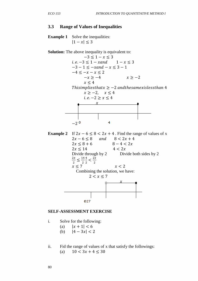
ECO 153 INTRODUCTION TO QUANTITATIVE METHOD I
80
3.3 Range of Values of Inequalities Example 1 Solve the inequalities: |1 − �| ≤ 3 Solution: The above inequality is equivalent to: −3 ≤ 1 − � ≤ 3 0. 2. −3 ≤ 1 − ��*(1 − � ≤ 3 −3 − 1 ≤ −��*( − � ≤ 3 − 1 −4 ≤ −� − � ≤ 2 −� ≥ −4� ≥ −2 � ≤ 4 ℎ0)0%6@02).ℎ�.� ≥ −2�*(.ℎ2)�%2�0)@2)).ℎ�*4 � ≥ −2,� ≤ 4 0. 2. −2 ≥ � ≤ 4 � −2 Example 2 If 2� − 6 ≤ 8 < 2� + 4. Find the range of values of x 2� − 6 ≤ 8�*(8 < 2� + 4 2� ≤ 8 + 68 − 4 < 2� 2� ≤ 144 < 2� Divide through by 2 Divide both sides by 2
��� ≤ �4
�4� <
���
� ≤ 7� < 2 Combining the solution, we have: 2 < � ≤ 7 �
SELF-ASSESSMENT EXERCISE i. Solve for the following:
(a) |� + 1| < 6 (b) |4 − 3�| < 2
ii. Fid the range of values of x that satisfy the followings: (a) 10 < 3� + 4 ≤ 30

ECO 153 MODULE 2
81
(b) −5 ≤ 3� − 14 ≤ 0 (c) 3 < 11 − � < 11 (d) 6 < 4� − 2 < 12
iii. Find he largest possible value of x that satisfy the followings: (a) � + 7 ≤ 13 (b) 3� − 7 ≤ 6
iv. Find the smallest possible of x that satisfy the followings: (a) � + 6 > 4 (b) 2 ≥ 14 − �
4.0 CONCLUSION
Inequalities involve the use of signs to compare two unequal expression or numbers. Solutions to inequality problems or equation follow similar approach with the linear equation. An inequality expression having more than one inequality sign is bound to have more than one range of value. 5.0 SUMMARY The use of signs in mathematics is meant to compare the magnitude of one expression or quantity with another. Mathematicians use both equality and inequality signs to compare and contrast values so as to be able to arrive at a conclusion. 6.0 TUTOR-MARKED ASSIGNMENT 1. Assume x is a whole number and x is an integer. For each of the
following list, the set of value of x. (a) 4 < � ≤ 7 (b) −5 < � < 1 (c) 5 < � + 9 (d) 6� > 4 (e) −9 ≤ � < 4
2. Find the range of values of x that satisfy each of the following: (a) −1 ≤ 4� + 15 < 23 (b) 0 ≤ 15 − � ≤ 10 (c) |2� − 3| ≤ 5

ECO 153 INTRODUCTION TO QUANTITATIVE METHOD I
82
7.0 REFERENCES/FURTHER READING
Murray, L. (1987). Progress in Mathematics. Lagos: Stanley Thomas Publishers Limited.
Norton, F. G. J. (2000). Ordinary Level Mathematics. Ibadan:
Heinemann Education Books. Usman, A. S. (2005). Business Mathematics. Ibadan: Apex Books
Limited.
ECO 153 MODULE 3
83
MODULE 3 SET THEORY Unit 1 Meaning and Classification of Sets Unit 2 Set Notations and Terminologies Unit 3 Laws of Sets Operation Unit 4 Venn Diagrams Unit 5 Application of Sets to Managerial and Economic Problems UNIT 1 MEANING AND CLASSIFICATION OF SETS CONTENTS 1.0 Introduction 2.0 Objectives 3.0 Main Content 3.1 General Overview 3.2 Definition and Representation of Sets 3.3 Classification and Properties of Sets 4.0 Conclusion 5.0 Summary 6.0 Tutor-Marked Assignment 7.0 References/Further Reading 1.0 INTRODUCTION Mathematics just like any other analytical science has a way of classifying information or data into classes or groups. This is usually done to present the information in compact form as well as to identify various component of each unit or group. This is applicable in everyday activities. Some modern shops are divided into different units or sections while in offices there are different departments, units, division, etc. the collection or aggregate of objects in a particular class is what is technically called ‘Set’ in mathematics. Therefore we can have set of alphabets in English language, set of students in a class or classes, set of days in a week, set of odd numbers, set of perfect squares, set of students offering, a course set of workers in different units of an organisation, set of accountants etc. 2.0 OBJECTIVES At the end of this unit, you should be able to: • define the term “Sets” • outline and explain the various representation of sets • list the various classification of sets
ECO 153 INTRODUCTION TO QUANTITATIVE METHOD I
84
• state the basic properties of sets.
3.0 MAIN CONTENT 3.1 General Overview
Generally, mathematicians call any-well defined classes “a set” and by well-defined we mean that we must be able to decide definitely whether any object does or does not belong to that set. These objects may be a group of (distinct) numbers, variables, parameter or something else that has properties or identification and distinctions from others. Thus all the students enrolled in a particular economics course can be considered a set, just as the positive integers (1, 2, 3…) can form a set. Animate, inanimate, tangible as well as intangible objects can be conceptualised to form a set. SELF-ASSESSMENT EXERCISE i. Why do mathematicians classify objects into sets? ii. Outline five different set of objects and give an example of a
member in each set.
3.2 Definition and Representation of Sets A set is any well-defined aggregate or collection of objects that are all different which a member of a group becomes either by following a particular rule or by simple imposition. The objects which belong to a set are called its elements or members of the set. A set is normally denoted by capital letters while the elements are represented by small letters. For example: A = {a, b, c, d, e, f} X = {2, 4, 6, 8, 10…}
Therefore, we say that aЄA, cЄA, 2ЄX, 6ЄX, bЄX, 4ЄA. This implied that a is an element of A, c is an element of A, 2 is an element of X, 6 is an element of X, but b is not an element of X neither is 4 an element of A.
The number of elements contained in a set is simply called the number of elements (n). For instance, in the previous example n(A) = 6 because there are six elements in A. However, the number of elements in X is not defined.

ECO 153 MODULE 3
85
There are two major ways of representing sets namely: (i) Roster method (ii) Descriptive method.
Roster method is the one in which each element is listed in an enclosed bracket. It is sometimes called tabulation method. Example: B= {x, y, z} which means the elements of B are x, y and z. The roster method states categorically all the elements in a set.
The descriptive method or the set builder rotation is the use of signs to specify the elements in a set. It is a method in which set listings are governed by particular rules indicating the range of elements contained in a set. For example:
H = {h: 3 ≤ h < 10} P = {x: x = 0, 1, 2, 3,…15}
The set H has its elements as 3, 4, 5, 6, 7, 8 and 9 since h ≥ 3 and the same h < 10. Likewise, Set P has its elements as 0, 1, 2, 3, 4, 5, 6, 7, 8, 9, 10, 11, 12, 13, 14 and 15. The three dots imply the continuation of the already existing pattern. SELF-ASSESSMENT EXERCISE
i. List the elements of the following sets:
(i) Notes denominations in the Nigeria’s currency (ii) Banks in Nigeria (iii) Even numbers less than 13 (iv) Prime numbers less than 20 (v) Multiples of 4 less than 15 (vi) Alphabets in English Language (vii) Multiples of 5 (viii) Months in a year (ix) Days in a week (x) Prime factors of 120.
ii. Find out the number of elements in each of the sets stated 1(i-x) above.
ECO 153 INTRODUCTION TO QUANTITATIVE METHOD I
86
3.3 Classification and Properties of Sets Sets are generally classified into two namely: (i) Finite Set (ii) Infinite Set
This classification is premised around the number of elements a set contains. A set is finite when it has a definite number of elements. For example, J = {x/2 < x < 5} J is a set of real numbers greater than 2 but less than 5 so J = {3}. Another example is S = {2, 3, 4}. Finite sets are always denumerable (i.e. countable). This implies that their elements can be counted one by one in a sequential order. Given that K = {even numbers between 2 and 16}, K is another example of finite set since its elements are countable i.e. K = {2, 4, 6, 8, 10, 12, 14, 16}.
An infinite set is the one in which the number of elements is indefinite. Such sets do not have last element in their range of values or membership. Infinite sets are non-denumerable (i.e. their elements are uncountable). Examples include:
N = {Natural numbers} K = {Multiples of 4} I = {x/x is a positive integer}
In each of the sets N, K and I above, the elements of sets in each group is uncountable, therefore each set is said to be indefinite.
Properties of set refer to the qualities that all sets have in common. These properties are: (i) The collection of object must be well defined. This implies that
there is no ambiguity about a set. (ii) The order in which objects are arranged in a set is immaterial. For
example: A = {a, b, c, d}, B = {b, c, a, d}, the same number of identical
elements, although the order of the arrangement differs. The order of the arrangement is insignificant as much as the sets have the some elements, they are said to be the same.
(iii) The object in a set must be distinct. This implies that, no object can appear more than once. For instance: A = {Musa, Emeka, Tina, Emeka} is wrong because of the duplication of Emeka. Rather, A = {Musa, Emeka, Tina}.
ECO 153 MODULE 3
87
SELF-ASSESSMENT EXERCISE For each of the sets, which elements are listed in question 1 of self-assessment exercise above? Justify whether they are definite or indefinite. 4.0 CONCLUSION Set theory is an important component of mathematics that describes and analyses the classification of objects into groups or division for the purpose of carrying out some descriptive and quantitative analyses on the interrelationship of the membership of the group or set as well as the relationship with the elements of other groups or sets. 5.0 SUMMARY
Set is broadly defined as the collection of data objects. Objects refer to items that can be quantified as well as those that cannot be quantified. However the collection of the items must be well defined and distinct. The order in which the objects are arranged in the set is practically immaterial. Sets can be represented with the use of Roster method or descriptive method (set builder). While the Roster method presents the vivid elements that a set contains the descriptive method adopts the use of signs to describe the range of values contained as elements of a set. Sets are generally classified into two: Finite sets and Infinite sets. Finite sets contain a finite or definite number of elements while infinite sets contain indefinite or infinite number of elements. More terminologies and notations used, in set operations are discussed in the next unit. 6.0 TUTOR-MARKED ASSIGNMENT 1. List the elements of the following sets.
A {continents in the world} B {state capitals in Nigeria} C {natural numbers greater than 10} D {x: - 6 ≤ x < 6} E {courses in Nigerian University}
2. State whether each of the sets above is definite or indefinite. 3. Find out, where possible, the number of elements in each of sets
listed in (1) above.
ECO 153 INTRODUCTION TO QUANTITATIVE METHOD I
88
7.0 REFERENCES/FURTHER READING Chiang, A. C. (1984). Fundamental Methods of Mathematical
Economic. (3rd ed.). USA: McGraw-Hills Inc. Hardwood, C. L. (1978).Ordinary Level Mathematic. (6th ed.). Ibadan:
Heinemann Educational Books. Murray, L. (1987). Progress in Mathematics. London: Therues
Publishers Limited. Usman, A. S. (2005). Business Mathematics. Lagos: Apex Books
Limited.
ECO 153 MODULE 3
89
UNIT 2 SET NOTATIONS AND TERMINOLOGIES CONTENTS 1.0 Introduction 2.0 Objectives 3.0 Main Content 3.1 General Overview 3.2 Set Notations and Terminologies 4.0 Conclusion 5.0 Summary 6.0 Tutor-Marked Assignment 7.0 References/Further Reading 1.0 INTRODUCTION Similar to other aspects of mathematics, some terminologies are peculiar to set theory. These terminologies and their signs notations are the basic and conventional languages used in set theory. The commonest among those are Universal sets, Subset, Proper subset, Null or Empty set, Union of sets, Intersection of sets, and Complements of set etc. These terms along with other notations enable us to establish visual and mathematical relationship between sets. 2.0 OBJECTIVES At the end of this unit, you should be able to: • identify set notations and what they mean • solve some problems involving sets notations and terminologies. 3.0 MAIN CONTENT 3.1 General Overview
When two sets are compared with each other, several possible kinds of relationship may be observed. If two sets S1 and S2 are given as S1 = {2, 7, a, f} and S2 = {2, a, 7, f}. S1 and S2 are said to be equal i.e. (S1 = S2). Whenever the elements are different, the two sets are not equal.
Another kind of relationship is that one set may be a subset of another set. If S = {1, 3, 5, 7, 9} and T = {3, 7}, then T is a subset of S, because every element of T is also known as element of S.
At the other extreme, the ‘smallest’ possible subset of S is a set that contains no element at all such a set is called the null set, or empty set;
ECO 153 INTRODUCTION TO QUANTITATIVE METHOD I
90
donated by the symbol or { }. The null set is unique; there is only one such set in the whole world and it is considered as a subset of any set that can be conceived.
When two sets have no element in common at all, the two sets are said to be Disjoint. When they have element in common the element they have in common is known as the intersection of the sets.
The combination of elements of two sets without repetition of common elements is called the union the sets. The complement of a set on the other hand are the set of element found in the universal set (a set containing every other sets defined) but not found in the set whose complement is being sought.
SELF-ASSESSMENT EXERCISE
With appropriate illustration and examples, define each of the following terminologies in sets operation: (a) Subset (b) Union of sets (c) Intersection of sets (d) Empty or Null set (e) Complement of a set. 3.2 Set Notations and Terminologies
(a) Universal Sets Universal set is the set of all objects of interest to an investigator or researcher. It is usually denoted by µ or £. It is the totality of elements present in two or more sets. For example U = {all lecturers of all university in Nigeria}. U here is a set with large number of elements which is obtained as a result of the combination of a large number of smaller sets i.e. sets of lectures in each of the Nigerian University. Example: Given that:
A {positive integers less than 10} B {factors of 12} C {even numbers less than 13}
Provided that the sets A, B and C form a universal set, find the elements of the Universal set.
Solution: A = {1, 2, 3, 4, 5, 6, 7, 8, 9}
B = {1, 2, 3, 4, 6, 12, 12} C = {2, 4, 6, 8, 10, 12} ... µ = {1, 2, 3, 4, 5, 6, 7, 8, 9, 10, 12}.
ECO 153 MODULE 3
91
Note: µ is obtained by combining all elements in all the sets given, without repetition of any element.
(b) Union of Sets The union of sets is a new set formed through the combination of elements in two or more sets. To take the union two sets A and B mean to form a new set containing those elements (and only those elements) belonging to A or to B, or to both A and B. The union set is symbolised by AUB (read: A union B).
Example 1 If A = {3, 5, 7}, B = {2, 3, 4, 8}
Then Find AUB.
Solution AUB = {2, 3, 4, 5, 7, 8}
Note: This example illustrates the case in which two sets A and B are neither equal nor disjoint and in which neither is a subset of the other.
(c) Intersection of Sets The intersection of sets is a new set formed from elements common to the sets. It is the set of elements common to two or more sets, or the elements that are common to two or more sets. The intersection of two sets A and B is a new set which contains those elements (and only those elements) belonging to both A and B. The intersection set is symbolised by AnB (read; A intersection B).
Example: Given that:
A {prime number less than 20} B {even numbers less than 15} C {Multiples of 4 less than 15} Find AnB, BnC, AnC
Solution A = {2, 3, 5, 7, 11, 13, 17, 19} B = {2, 4, 6, 8, 10. 12, 14} C = {4, 8, 12} (i) AnB = {2} (ii) BnC = {4, 8, 12} (iii) AnC = { } or Ø -Empty set: That is, no element is common to sets A and C.
ECO 153 INTRODUCTION TO QUANTITATIVE METHOD I
92
(d) Subset and Proper Subset A set X is said to be a subset of another set Y (denoted by XCY) if and if only each element of X is an element of Y, for example, a set of students offering Economics is a subsets of students enrolled in the faculty of social science while the students in the social sciences are subset of the entire students enrolled in the University.
If S = {1, 3, 5,7, 9} and T = {3,7}, then T is a subset of S, because every element of T is also an element of S. Strictly we can say that T is a proper subset of S, for T does not contain every elements in S. Therefore every set is a subset of itself but not a proper subset of itself. Also, empty set is not a proper subset of any set. This implies that two equal sets are subset of one another and not a proper subset of one another.
Example: Given that A = {2, 3, 5, 7, 11, 13, 17, 19} B = {2, 4, 6, 8, 10, 12, 14} C = {4, 8, 12}
(a) Is B is proper subset of A? Why? (b) Is C a proper subset of B? Why? (c) List some proper subsets of B. (d) List all proper subsets of C.
Solution
(a) B is not a proper subset of A because not all elements of B are
found in A. (b) C is a proper subset of B because all elements of C are found in
B, with B containing some other elements outside the elements of B.
(c) The proper subsets of B are {4}, {8}, {12}, {4, 8}, {4, 12}, and so on. It can be shown that there are over 100 proper subsets of B.
(d) The proper subsets of C are {4}, {8}, {12}, {4, 8}, {4, 12}, {8, 12}, {4, 8, 12}. Note { } - empty set is not a proper subset of any set. The proper subsets of C is exhaustive i.e. we can list all the subsets of C.
(e) Null or Empty Set: A null set is a set that contains no element. It should be noted that, an empty set has no element. This implies that, if A is an empty set n(A) = 0. Empty set is symbolised as { } or Ø or and not {O} or {Ø}. It is wrong to connote empty set as {O} because if we do, it implies that the set has an element which is Zero. Similarly if A = {Ø}, A is not an empty set, what this connotes is that A has one element (i.e. n(A ) = 1) which is Ø. Therefore an empty set is either represent as Ø or { }.

ECO 153 MODULE 3
93
Example: A = {positive odd numbers} B = {positive even numbers}
Find AnB Solution
A = {1, 3, 5, 7, 9, 11, 13…} B = {2, 4, 6, 8, 10, 12, 14…}
... AnB = { } or Ø. This implies that there is no element common to sets A and B. In other words the intersection of sets A and B gives an empty set.
(e) Complement of Sets All the elements of the universal set which are not members of a set A form the set called complement of A, denoted by Ac or A1 for instance If µ or £= {1, 2, 3, 4, 5, 6} A = {1, 2, 4, 5} Then, Ac = A1 = {3, 6} (f) Difference of Sets The difference between two sets is technical called the relative complement. For instance, given the sets of A and B, the relative complement of A and B denoted by A – B implies the elements which belong to A but does not belong to B.
On the other hand, absolute complement a set refers to elements found in the universal set but not in the set whose complement is being sought. Given sets A, B and C forming the universal set µ, the absolute complement of A, Ac or A1 are elements in µ but not in A. Example: Given that µ = {1, 2, 3, 4 … 12} A = {1, 3, 5, 7, 10} B = {1, 4, 6, 9, 10} C = {2, 8, 9, 10, 11, 12}
Required: - Find (i) Bc (ii) A1 (iii) C1 (iv) B – A (v) A – C
Solution
(i) Bc or B1 = {2, 3, 5, 7, 8, 11, 12} (ii) A1 = {2, 4, 6, 8, 9, 11, 12} (iii) C1 = {1, 3, 4, 5, 6, 7}

ECO 153 INTRODUCTION TO QUANTITATIVE METHOD I
94
(iv) B – A = {4, 6, 9}. B–A Implies elements in B but not in A. (v) A – C = {1, 3, 5, 7}. A–C Implies elements in A but not in
C. Combine Examples: 1. Given that; A = {prime numbers less than 20}
B = {x1: 0 < x ≤15} C = {Even numbers less than 20}
Find: (a) µ (b) A1nC1 (c) n[(AnB)1UC1]
2. Given that; µ = {…-5, -4, -3, -2, -1, 0, 1, 2, 3…} X = {p: p ≤ 9} Y = {q: -15 < q < 12} Z = {r: r> 0}
(a) List the elements of X, Y and Z (b) Find (XUY)1nZ
Solution
1. A = {2, 3, 5, 7, 11, 13, 17, 19} B = {1, 2, 3, 4, 5, 6, 7, 8, 9, 10, 11, 12, 13, 14, 15} C = {2, 4, 6, 8, 10, 12, 14, 16, 18} (a) µ = AUBUC = {1, 2, 3, 4, 5, 6, 7, 8, 9, 10, 11, 12,13, 14,
15, 16, 18,19} (b) A1 = {1, 4, 6, 8, 9, 10, 12, 14, 15, 16, 18} C1 = {1, 3, 5, 7, 9, 11, 13, 15, 17, 19} ... A1nC1 = {1, 9, 15} (c) AnB = {2, 3, 5, 7, 11, 13} (AnB) 1 = {1, 4, 6, 8, 10, 12, 14, 15, 16, 17, 18, 19} C1 = {1, 3, 5, 7, 9, 11, 13, 15, 17, 19} ... (AnB)1UC1 = {1, 3, 4, 5, 6, 7, 8, 9, 10, 11, 12, 13, 14,
15, 16, 17, 18, 19} Hence, n[(AnB)UC] = 18 i.e. there are 18 elements in
(AnB)1UC1 2. µ = {…-5, -4, -3, -2, -1, 0, 1, 2, 3, 4, 5…} X = {9, 10, 11, 12, 13, 14, 15, 16…} Y = {-14, -13, -12, -11, -10, -9, -8, -7, -6, -5, -4, -3, -2, -1, 0, 1, 2,
3, 4, 5, 6, 7, 8, 9, 10, 11}. (XUY) = {-14, -13, -12, -11 …} (XUY) 1 = {… -16, -15} Z = {1, 2, 3, 4 …} ... Z 1 = {… -16, -15, -14 …0} ... (XUY)1 n Z1 = {… -16, -15}
ECO 153 MODULE 3
95
SELF-ASSESSMENT EXERCISE
i. Given the following: Universal set = {1, 2, 3…10}
A = {1, 2, 3, 4, 5, 6} B = {4, 5, 6, 7, 8}
Find: (a) AUB (b) AnB (c) B1
ii. Given the sets: S1 = {2, 4, 6}, S2 = {7, 26} S3 = {4, 2, 6} and S4 = {2, 4}, which of the following statements is/are true (a) S1 = S2 (b) S1 C S4 (c) 4 S4 (d) 5 S2 (e) S4 C S1
iii. If A = {all multiples of 3 less than 20} B = {all multiples of 6 less than 20} (a) List the elements of A (b) List the element of B (c) List the element of AUB (d) List the elements of AnB.
4.0 CONCLUSION Set notations are terminologies that are very essential in set theory. They enable us to establish the relationship among the elements of a set as well as the interactions between one set and the others. 5.0 SUMMARY Set notations are the signs and symbols used to draw relationship and conclusion among the elements of a set as well as the signs and symbols used to establish interrelationship between the elements of one set and the elements of the other.
Terminologies used in set theory include subsets and proper subsets, universal sets, empty sets intersection of two or more sets, union of two or more sets, complement of a sets difference of two sets, etc. These terminologies are peculiar languages, which are exclusively used in set theory as defined in the content of this unit.

ECO 153 INTRODUCTION TO QUANTITATIVE METHOD I
96
6.0 TUTOR-MARKED ASSIGNMENT 1. Write the following in set notation:
(a) The set of all real numbers greater than 27 (b) The set of all real numbers greater than 8 but less than 43.
2. Enumerate all the subsets of the set {a, b, c}. How many subsets are there altogether? 3. If E = {1, 2, 3, 4, 5, 6, 7, 8} A = {1, 2, 4, 8} B = {1, 3, 5, 7} C = {2, 4, 6, 8}
List the elements of: (i) A1 (ii) B1 (iii) C1UA1 (iv) AnB (v) B1nC1
4. Given that; µ = {-5, -4, -3, -2, -1, 0, 1, 2, 3…} P = {x: -8 < X < 8} R = {y: y < 12}
Required (a) P1 (b) R1 (c) P1nR1
7.0 REFERENCES/FURTHER READING Chiang, A. C. (1984). Fundamental Methods of Mathematical
Economic. (3rd ed.). USA: McGraw-Hills Inc. Harwood, C. L. (1978). Ordinary Level Mathematic. (6th ed.). Ibadan:
Heinemann Educational Books. Murray, L. (1987). Progress in Mathematics. London: Thornes
Publishers Limited.
ECO 153 MODULE 3
97
UNIT 3 LAWS OF SET OPERATIONS CONTENTS 1.0 Introduction 2.0 Objectives 3.0 Main Content 3.1 General Overview 3.2 Laws of Set Operations 4.0 Conclusion 5.0 Summary 6.0 Tutor-Marked Assignment 7.0 References/Further Reading 1.0 INTRODUCTION
Like every other mathematical principles or theorem, the set theory is guided by some laws. These laws are meant to establish certain identities that may result from the use of various set notations. The laws have been put to test using various sets and elements and they have been validated over time. 2.0 OBJECTIVES At the end of this unit, you should be able to: • outline the basic laws in set operations • use some sets to confirm each of the laws. 3.0 MAIN CONTENT 3.1 General Overview Set notations exhibit certain relationship interrelationship. This relationship results into some conventional set properties and laws. Among these laws are Idempotent law/property, commutative law/property, associative law/property, identity property, complement property and De Morgan’s law. 3.2 Laws of Set Operations (a) Idempotent Properties: This property states that the union and
intersection of the same set gives the set. AUA = A AnA = A
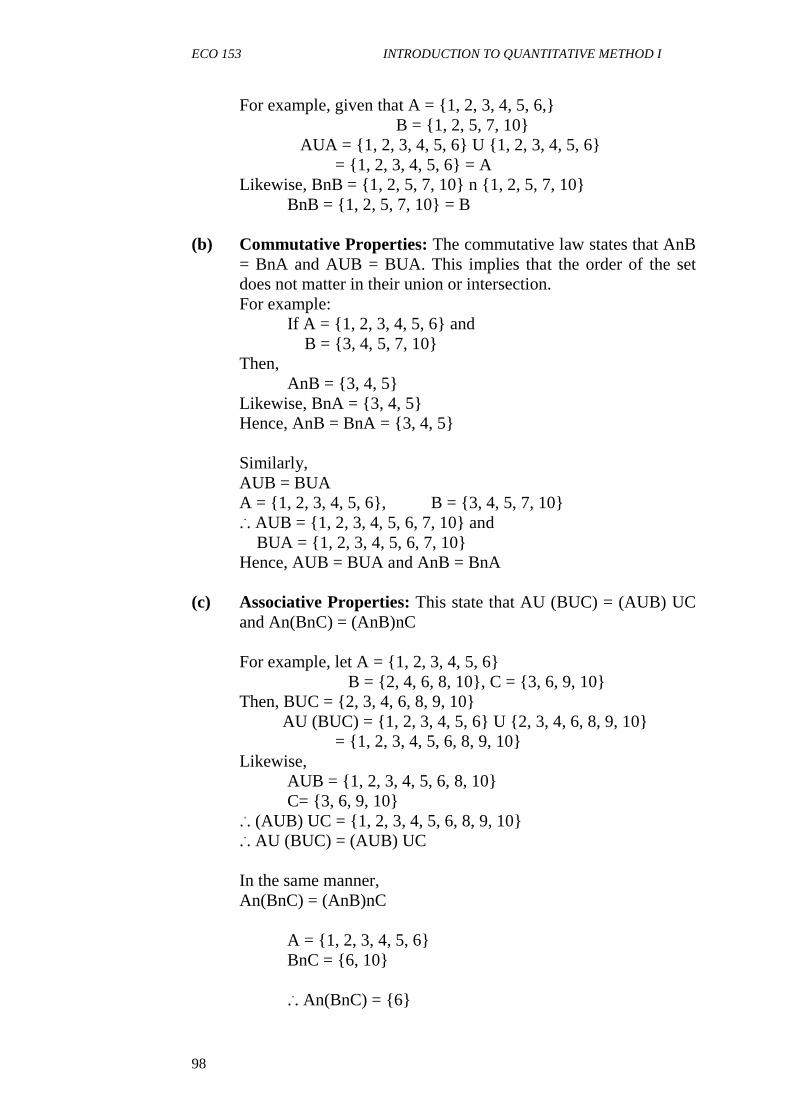
ECO 153 INTRODUCTION TO QUANTITATIVE METHOD I
98
For example, given that A = {1, 2, 3, 4, 5, 6,} B = {1, 2, 5, 7, 10}
AUA = {1, 2, 3, 4, 5, 6} U {1, 2, 3, 4, 5, 6} = {1, 2, 3, 4, 5, 6} = A
Likewise, BnB = {1, 2, 5, 7, 10} n {1, 2, 5, 7, 10} BnB = {1, 2, 5, 7, 10} = B (b) Commutative Properties: The commutative law states that AnB
= BnA and AUB = BUA. This implies that the order of the set does not matter in their union or intersection. For example:
If A = {1, 2, 3, 4, 5, 6} and B = {3, 4, 5, 7, 10}
Then, AnB = {3, 4, 5}
Likewise, BnA = {3, 4, 5} Hence, AnB = BnA = {3, 4, 5} Similarly, AUB = BUA A = {1, 2, 3, 4, 5, 6}, B = {3, 4, 5, 7, 10} ... AUB = {1, 2, 3, 4, 5, 6, 7, 10} and BUA = {1, 2, 3, 4, 5, 6, 7, 10} Hence, AUB = BUA and AnB = BnA
(c) Associative Properties: This state that AU (BUC) = (AUB) UC and An(BnC) = (AnB)nC For example, let A = {1, 2, 3, 4, 5, 6} B = {2, 4, 6, 8, 10}, C = {3, 6, 9, 10} Then, BUC = {2, 3, 4, 6, 8, 9, 10} AU (BUC) = {1, 2, 3, 4, 5, 6} U {2, 3, 4, 6, 8, 9, 10} = {1, 2, 3, 4, 5, 6, 8, 9, 10} Likewise, AUB = {1, 2, 3, 4, 5, 6, 8, 10} C= {3, 6, 9, 10} ... (AUB) UC = {1, 2, 3, 4, 5, 6, 8, 9, 10}
... AU (BUC) = (AUB) UC In the same manner, An(BnC) = (AnB)nC
A = {1, 2, 3, 4, 5, 6}
BnC = {6, 10}
... An(BnC) = {6}
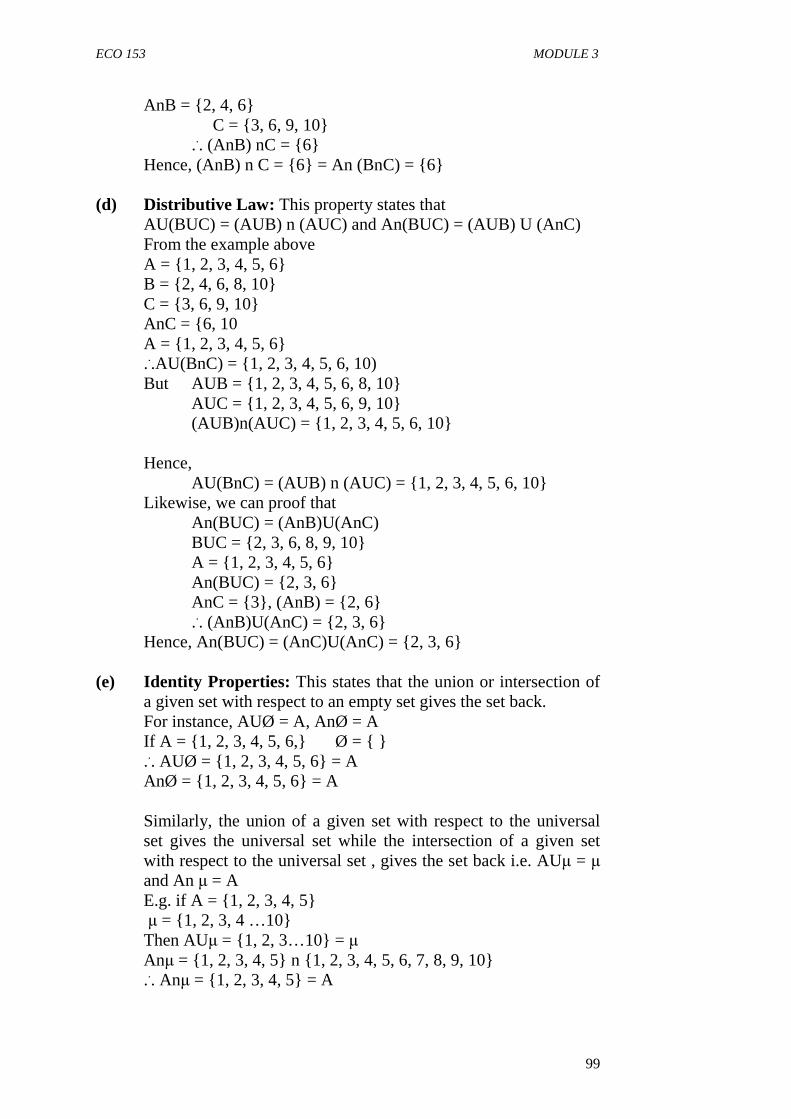
ECO 153 MODULE 3
99
AnB = {2, 4, 6} C = {3, 6, 9, 10} ... (AnB) nC = {6}
Hence, (AnB) n C = {6} = An (BnC) = {6} (d) Distributive Law: This property states that AU(BUC) = (AUB) n (AUC) and An(BUC) = (AUB) U (AnC)
From the example above A = {1, 2, 3, 4, 5, 6} B = {2, 4, 6, 8, 10} C = {3, 6, 9, 10} AnC = {6, 10 A = {1, 2, 3, 4, 5, 6} ...AU(BnC) = {1, 2, 3, 4, 5, 6, 10) But AUB = {1, 2, 3, 4, 5, 6, 8, 10}
AUC = {1, 2, 3, 4, 5, 6, 9, 10} (AUB)n(AUC) = {1, 2, 3, 4, 5, 6, 10}
Hence, AU(BnC) = (AUB) n (AUC) = {1, 2, 3, 4, 5, 6, 10}
Likewise, we can proof that An(BUC) = (AnB)U(AnC) BUC = {2, 3, 6, 8, 9, 10} A = {1, 2, 3, 4, 5, 6}
An(BUC) = {2, 3, 6} AnC = {3}, (AnB) = {2, 6} ... (AnB)U(AnC) = {2, 3, 6}
Hence, An(BUC) = (AnC)U(AnC) = {2, 3, 6}
(e) Identity Properties: This states that the union or intersection of a given set with respect to an empty set gives the set back. For instance, AUØ = A, AnØ = A If A = {1, 2, 3, 4, 5, 6,} Ø = { } ... AUØ = {1, 2, 3, 4, 5, 6} = A AnØ = {1, 2, 3, 4, 5, 6} = A Similarly, the union of a given set with respect to the universal set gives the universal set while the intersection of a given set with respect to the universal set , gives the set back i.e. AUµ = µ and An µ = A E.g. if A = {1, 2, 3, 4, 5} µ = {1, 2, 3, 4 …10} Then AUµ = {1, 2, 3…10} = µ Anµ = {1, 2, 3, 4, 5} n {1, 2, 3, 4, 5, 6, 7, 8, 9, 10} ... Anµ = {1, 2, 3, 4, 5} = A
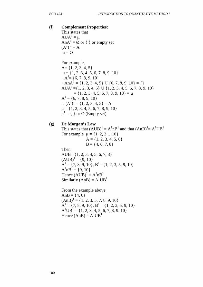
ECO 153 INTRODUCTION TO QUANTITATIVE METHOD I
100
(f) Complement Properties: This states that
AUA 1 = µ AnA1 = Ø or { } or empty set (A1) 1 = A µ = Ø For example, A= {1, 2, 3, 4, 5} µ = {1, 2, 3, 4, 5, 6, 7, 8, 9, 10} ...A1= {6, 7, 8, 9, 10} ...AnA1 = {1, 2, 3, 4, 5} U {6, 7, 8, 9, 10} = {} AUA 1 ={1, 2, 3, 4, 5} U {1, 2, 3, 4, 5, 6, 7, 8, 9, 10} = {1, 2, 3, 4, 5, 6, 7, 8, 9, 10} = µ A1 = {6, 7, 8, 9, 10} ... (A1)1 = {1, 2, 3, 4, 5} = A µ = {1, 2, 3, 4, 5, 6, 7, 8, 9, 10} µ1 = { } or Ø (Empty set)
(g) De Morgan’s Law This states that (AUB)1 = A1nB1 and that (AnB)1= A1UB1
For example µ = {1, 2, 3 …10} A = {1, 2, 3, 4, 5, 6}
B = {4, 6, 7, 8} Then AUB= {1, 2, 3, 4, 5, 6, 7, 8} (AUB)1 = {9, 10} A1 = {7, 8, 9, 10}, B1= {1, 2, 3, 5, 9, 10} A1nB1 = {9, 10} Hence (AUB)1 = A1nB1
Similarly (AnB) = A1UB1
From the example above AnB = {4, 6} (AnB)1 = {1, 2, 3, 5, 7, 8, 9, 10} A1 = {7, 8, 9, 10}, B1 = {1, 2, 3, 5, 9, 10} A1UB1 = {1, 2, 3, 4, 5, 6, 7, 8, 9. 10} Hence (AnB) = A1UB1
ECO 153 MODULE 3
101
SELF-ASSESSMENT EXERCISE
i. Which of the following statement(s) is/are valid? (a) AUA = A (b) AnA = A (c) AUØ = A (d) AUµ = U (e) AnØ = Ø (f) Anµ = A (g) The complement of A1 is A (i.e. (A1)1=A) (h) (BnC) = B1n C1 (i) AU(BUC) = An(BnC) (j) An (BUC) = (AnB)U(AnC)
ii. Given A = {4, 5, 6}, B = {3, 4, 6, 7} and C = {2, 3, 6}, verify: (a) Associative law (b) Distributive law (c) De Morgan’s law
4.0 CONCLUSION Rules and laws in set theory are designed to show interrelationship between/among the set notations. Some of the rules or properties highlighted above have been proved and validated using some sets information. 5.0 SUMMARY This unit focused on the basic law in set operations especially those that have to do with union, intersection and complements of set. The laws allows for clear understanding about the interrelationship among the major set notations (union, complement and intersection). 6.0 TUTOR-MARKED ASSIGNMENT 1. Verify De Morgan’s law using the sets below: µ = {1, 2, 3, 4 … 16} A = {1, 2, 3, 4, 5, 6, 7, 8, 9} B = {8, 9, 10, 11, 12} 2. Given that A= {0, 1, 2, 3}; B= {5, 6, 7} Verify whether each of the following is true or false
(a) A1nB1 = (AUB)1 (b) A1nB1 = Ø (c) AU(BnC) = (AUB) n (AUC) (d) (B1)1 = B.
ECO 153 INTRODUCTION TO QUANTITATIVE METHOD I
102
3. Verify De Morgan’s law using the sets below µ = {1, 2, 3, 4…16} A = {1, 2, 3… 9} B = {8, 9, 10, 11, 12} 7.0 REFERENCES/FURTHER READING Chiang, A. C. (1984). Fundamental Methods of Mathematical
Economic. (3rd ed.). USA: McGraw-Hills Inc. Murray, L. (1987). Progress in Mathematics. London: Therues
Publishers Limited. Usman, A. S. (2005). Business Mathematics. Lagos: Apex Books
Limited.
ECO 153 MODULE 3
103
UNIT 4 VENN DIAGRAM CONTENTS 1.0 Introduction 2.0 Objectives 3.0 Main Content 3.1 General Overview 3.2 Simple Set Problem involving Venn Diagram 4.0 Conclusion 5.0 Summary 6.0 Tutor-Marked Assignment 7.0 References/Further Reading 1.0 INTRODUCTION The use of diagram to represent information is a common phenomenon in Mathematics and other allied sciences. You must have been conversant with the tree diagram in probability histogram, pie charts, bar charts, in statistics and so on. Diagrams in form of figures, charts, graphs and free hand sketches are illustrative tools used in mathematics to establish vivid relationship among variables of interest. Set theory is not excluded in this category. Information in sets is also provided in diagrams called the Venn diagram. 2.0 OBJECTIVES At the end of this unit, you should be able to: • explain the relevance of Venn diagram to set theory • solve problems in set theory using Venn diagram • solve word-problems involving set theory with the use of Venn
diagrams. 3.0 MAIN CONTENT 3.1 General Overview
Venn diagrams consist of oval shapes representing independent and interrelated sets drawn in a rectangular space, which represents the universal set. It is meant to establish relationship and connections between different set units as well as the interrelationship between the sets and universal set.
The diagram showing this relationship (Venn diagram) was invented by an English mathematician known as John Venn (1834-1923). He used

ECO 153 INTRODUCTION TO QUANTITATIVE METHOD I
104
µ
µ
B
ovals to represent sets, and the ovals overlapped if the sets had any elements in common. Thus, the relationship between A and B is illustrated as:
If there is no element common to A and B, the Venn diagram appears thus:
However, if A contains every element in B, that is a proper subset of B, the Venn diagram appears as follow. �
�
A
A B
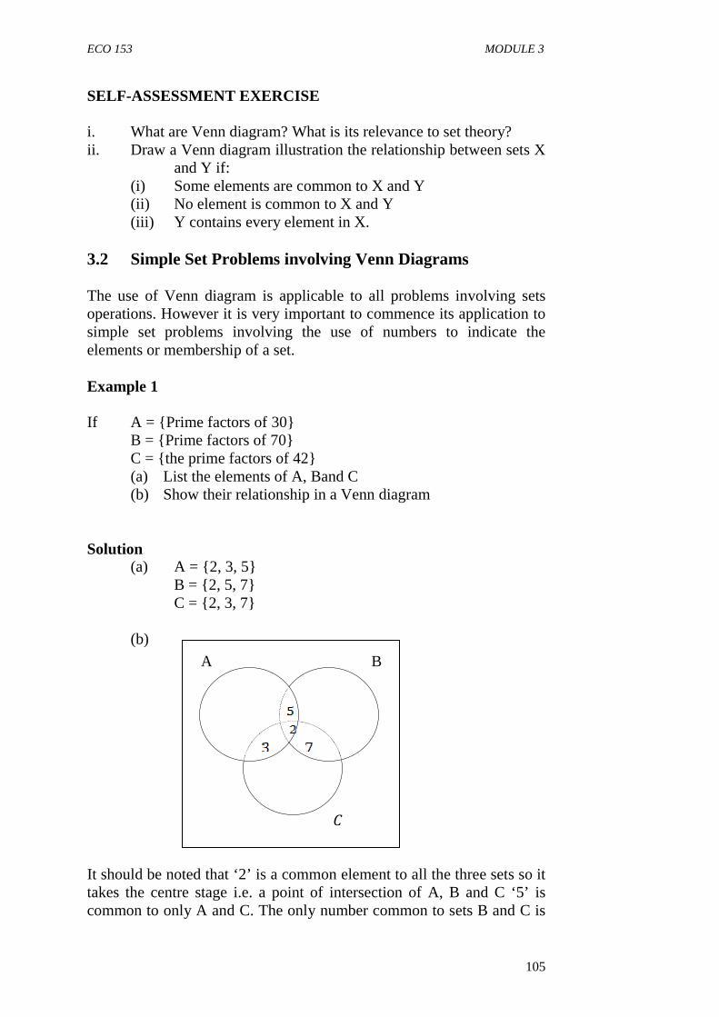
ECO 153 MODULE 3
105
SELF-ASSESSMENT EXERCISE i. What are Venn diagram? What is its relevance to set theory? ii. Draw a Venn diagram illustration the relationship between sets X
and Y if: (i) Some elements are common to X and Y (ii) No element is common to X and Y (iii) Y contains every element in X.
3.2 Simple Set Problems involving Venn Diagrams The use of Venn diagram is applicable to all problems involving sets operations. However it is very important to commence its application to simple set problems involving the use of numbers to indicate the elements or membership of a set.
Example 1
If A = {Prime factors of 30} B = {Prime factors of 70} C = {the prime factors of 42}
(a) List the elements of A, Band C (b) Show their relationship in a Venn diagram
Solution (a) A = {2, 3, 5}
B = {2, 5, 7} C = {2, 3, 7}
(b)
� It should be noted that ‘2’ is a common element to all the three sets so it takes the centre stage i.e. a point of intersection of A, B and C ‘5’ is common to only A and C. The only number common to sets B and C is
A B
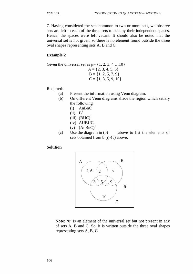
ECO 153 INTRODUCTION TO QUANTITATIVE METHOD I
106
7. Having considered the sets common to two or more sets, we observe sets are left in each of the three sets to occupy their independent spaces. Hence, the spaces were left vacant. It should also be noted that the universal set is not given, so there is no element found outside the three oval shapes representing sets A, B and C.
Example 2 Given the universal set as µ= {1, 2, 3, 4 …10} A = {2, 3, 4, 5, 6} B = {1, 2, 5, 7, 9} C = {1, 3, 5, 9, 10}
Required:
(a) Present the information using Venn diagram. (b) On different Venn diagrams shade the region which satisfy the following
(i) AnBnC (ii) B1 (iii) (BUC)1 (iv) AUBUC (v) (AnBnC)1
(c) Use the diagram in (b) above to list the elements of sets obtained from b (i)-(v) above.
Solution 2 7 3 5 1, 9 8 10
�
Note: ‘8’ is an element of the universal set but not present in any of sets A, B and C. So, it is written outside the three oval shapes representing sets A, B, C.
A B
4, 6
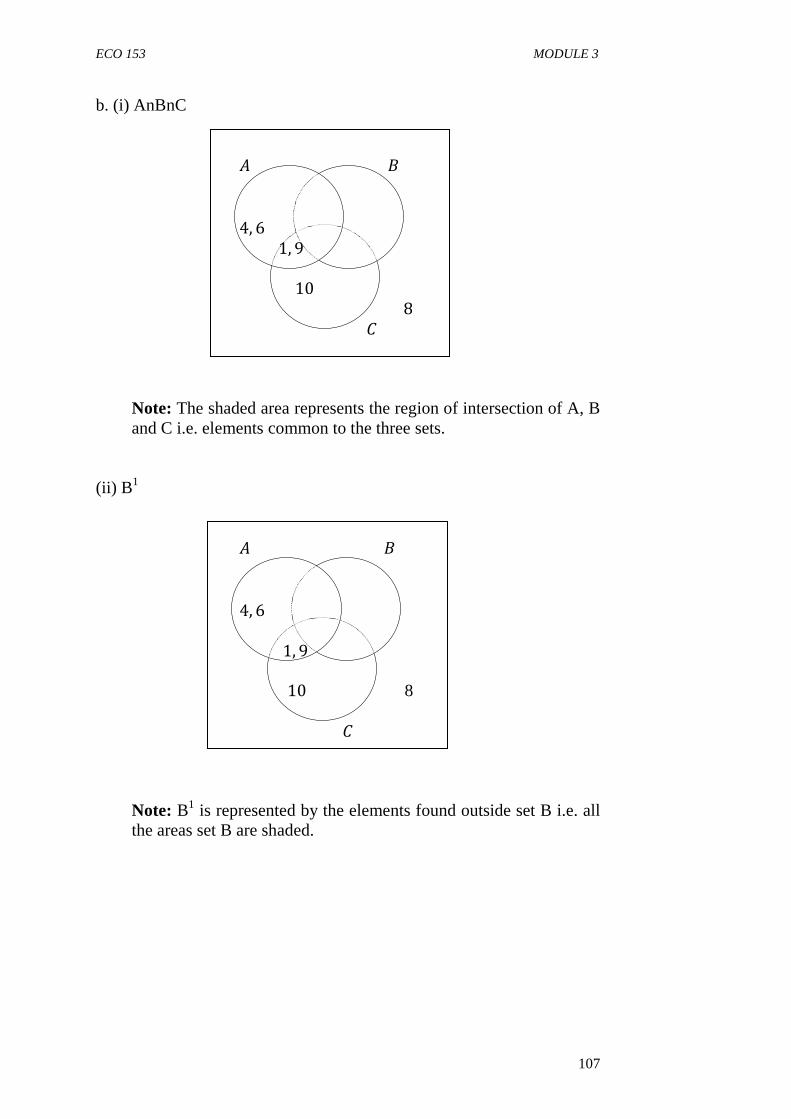
ECO 153 MODULE 3
107
b. (i) AnBnC �� 4, 6 1, 9 10
8 �
Note: The shaded area represents the region of intersection of A, B and C i.e. elements common to the three sets.
(ii) B1
�� 4, 6 1, 9 10 8
�
Note: B1 is represented by the elements found outside set B i.e. all the areas set B are shaded.
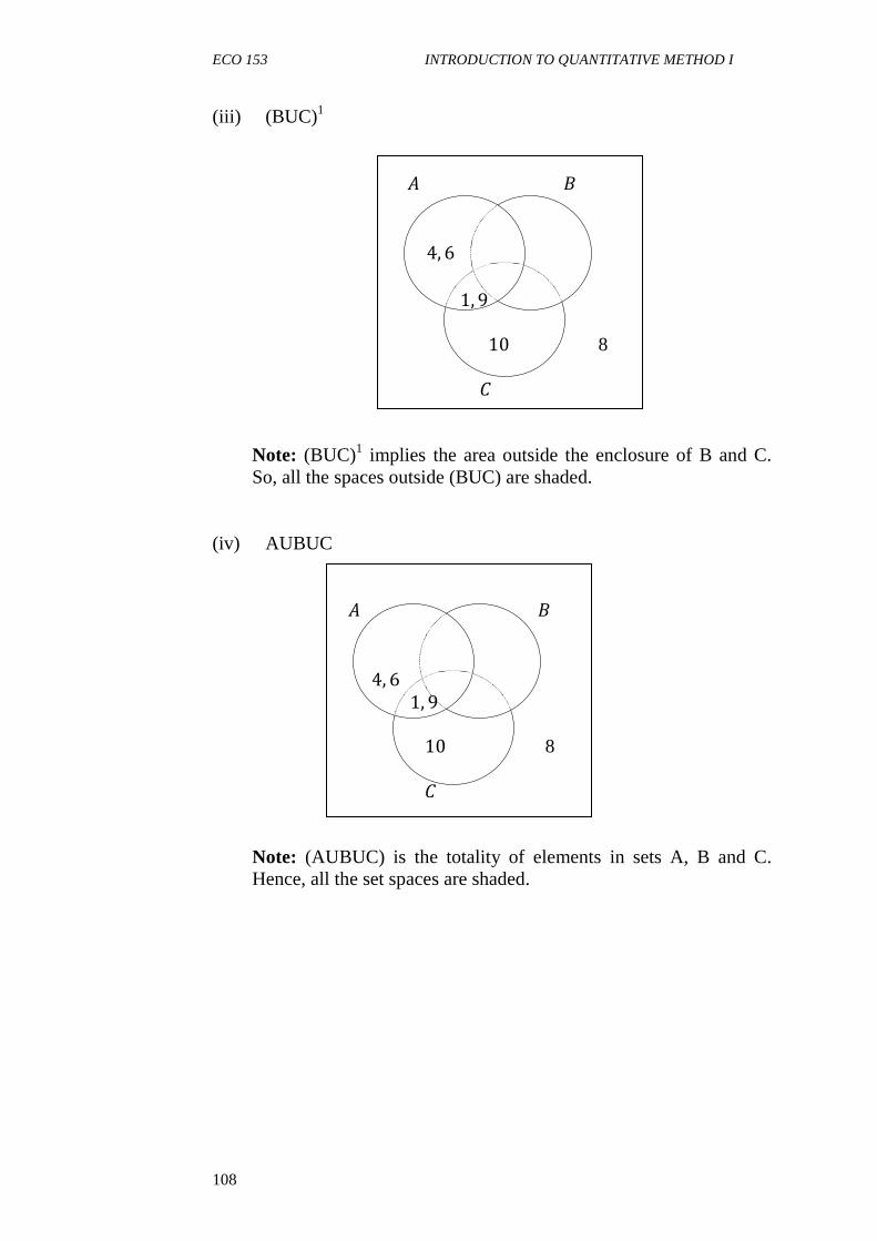
ECO 153 INTRODUCTION TO QUANTITATIVE METHOD I
108
(iii) (BUC)1
�� 4, 6 1, 9 10 8
�
Note: (BUC)1 implies the area outside the enclosure of B and C. So, all the spaces outside (BUC) are shaded.
(iv) AUBUC �� 4, 6 1, 9 10 8
�
Note: (AUBUC) is the totality of elements in sets A, B and C. Hence, all the set spaces are shaded.

ECO 153 MODULE 3
109
(v) (AnBnC)1
�� 4, 6 1, 9 10 8
�
Note: (AnBnC)1 implies the area outside (AnBnC). Hence the entire space is shaded with the exception of (AnBnC).
C (i) AnBnC = {5} (ii) B1 = {3, 4, 6, 8, 10} (iii) (BUC)1 = {4, 6, 8} (iv) AUBUC = {1, 2, 3, 4, 5, 6, 7, 9, 10} (v) (AnBnC)1 = {1, 2, 3, 4, 6, 7, 9, 10} SELF-ASSESSMENT EXERCISE i. Given that A = {all prime numbers between 10 and 30} B = {all even numbers between 9 and 29} C = {all multiples of 3 between 10 and 29}
Required: (a) List the elements of each set and draw a Venn diagram showing the relationship among the sets.
(b) In separate Venn diagrams, show the region that satisfy each of
(i) AU(BnC) (ii) (AnB)UC (c) List the elements of b(i) and b(ii) above (d) Is AU(BnC) = (AnB)UC? What do you think is responsible for this?
ii. If P and Q are sets, using a Venn diagram, shade the following relationship on different diagrams (a) PnQ (b) PUQ (c) P1 (d) Q1
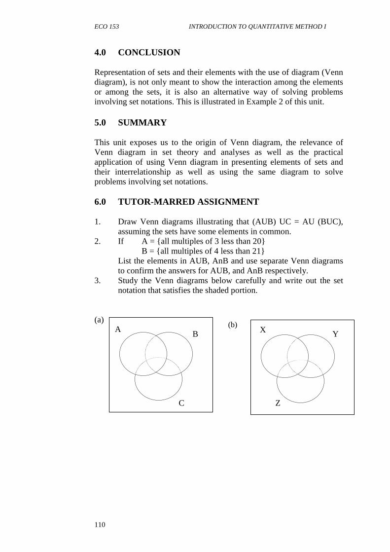
ECO 153 INTRODUCTION TO QUANTITATIVE METHOD I
110
(b)
4.0 CONCLUSION Representation of sets and their elements with the use of diagram (Venn diagram), is not only meant to show the interaction among the elements or among the sets, it is also an alternative way of solving problems involving set notations. This is illustrated in Example 2 of this unit. 5.0 SUMMARY This unit exposes us to the origin of Venn diagram, the relevance of Venn diagram in set theory and analyses as well as the practical application of using Venn diagram in presenting elements of sets and their interrelationship as well as using the same diagram to solve problems involving set notations. 6.0 TUTOR-MARRED ASSIGNMENT 1. Draw Venn diagrams illustrating that (AUB) UC = AU (BUC),
assuming the sets have some elements in common. 2. If A = {all multiples of 3 less than 20} B = {all multiples of 4 less than 21} List the elements in AUB, AnB and use separate Venn diagrams
to confirm the answers for AUB, and AnB respectively. 3. Study the Venn diagrams below carefully and write out the set
notation that satisfies the shaded portion. (a)
A B
C
X Y
Z
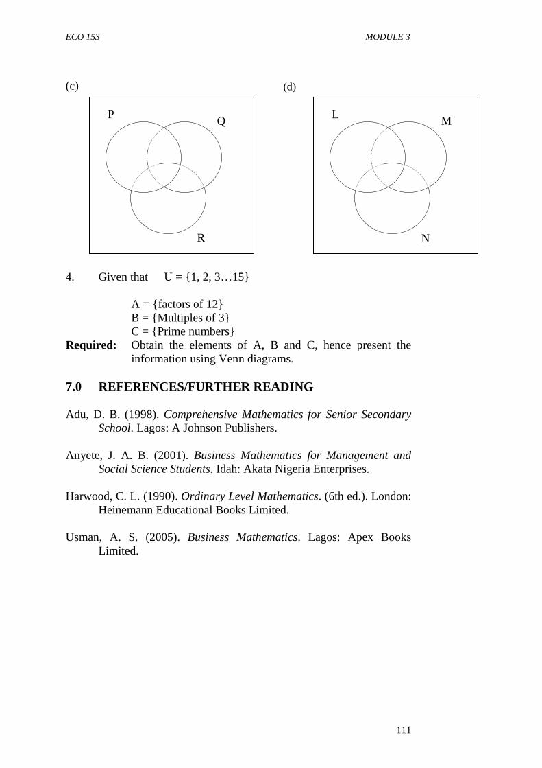
ECO 153 MODULE 3
111
(c)
4. Given that U = {1, 2, 3…15}
A = {factors of 12} B = {Multiples of 3} C = {Prime numbers} Required: Obtain the elements of A, B and C, hence present the
information using Venn diagrams. 7.0 REFERENCES/FURTHER READING
Adu, D. B. (1998). Comprehensive Mathematics for Senior Secondary
School. Lagos: A Johnson Publishers. Anyete, J. A. B. (2001). Business Mathematics for Management and
Social Science Students. Idah: Akata Nigeria Enterprises. Harwood, C. L. (1990). Ordinary Level Mathematics. (6th ed.). London:
Heinemann Educational Books Limited. Usman, A. S. (2005). Business Mathematics. Lagos: Apex Books
Limited.
(d)
P Q
R
L M
N
ECO 153 INTRODUCTION TO QUANTITATIVE METHOD I
112
UNIT 5 APPLICATION OF SETS (VENN DIAGRAM) TO MANAGERIAL AND ECONOMIC PROBLEMS CONTENTS 1.0 Introduction 2.0 Objectives 3.0 Main Content 3.1 General Overview 3.2 Solving Practical Problems using Venn Diagrams 4.0 Conclusion 5.0 Summary 6.0 Tutor-Marked Assignment 7.0 References/Further Reading 1.0 INTRODUCTION The use of Venn diagram is not limited to simple set problems in which element of a set have already being identified. It is equally applicable to real-life problems in which the numbers of element making up a group or set is identified. 2.0 OBJECTIVE At the end of this unit, you should be able to: • apply Venn diagram to solve day to day problem involving two
or three sets. 3.0 MAIN CONTENT 3.1 General Overview
In our day to day activities, we are confronted with categorisation of people or objects in different classes or division. In the course of doing this, there may be overlapping of one element appearing in two or more sets. For instance, students in a class may be able to speak English language or French fluently. Among these set of students, some may be able to speak the two languages and some may not be able to speak any of them fluently. In the course of analysing this, there may be a need to introduce Venn diagram. Another example is the elective courses taken by students in higher institutions. For example, if course A, B and C are made available as elective courses. Some students may offer one of the courses; some offer
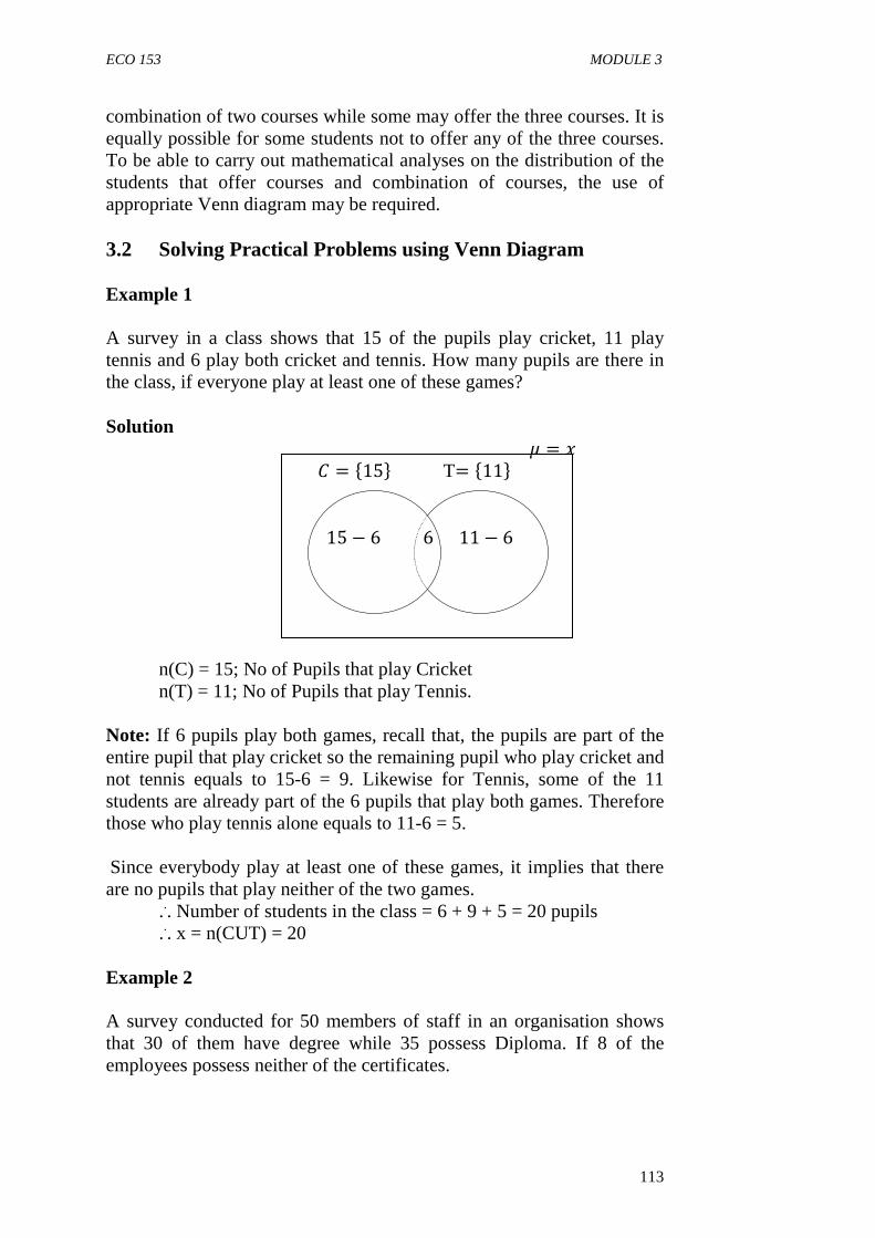
ECO 153 MODULE 3
113
combination of two courses while some may offer the three courses. It is equally possible for some students not to offer any of the three courses. To be able to carry out mathematical analyses on the distribution of the students that offer courses and combination of courses, the use of appropriate Venn diagram may be required. 3.2 Solving Practical Problems using Venn Diagram
Example 1 A survey in a class shows that 15 of the pupils play cricket, 11 play tennis and 6 play both cricket and tennis. How many pupils are there in the class, if everyone play at least one of these games? Solution � = � � = �15� T= �11� 15 − 6611 − 6
n(C) = 15; No of Pupils that play Cricket n(T) = 11; No of Pupils that play Tennis.
Note: If 6 pupils play both games, recall that, the pupils are part of the entire pupil that play cricket so the remaining pupil who play cricket and not tennis equals to 15-6 = 9. Likewise for Tennis, some of the 11 students are already part of the 6 pupils that play both games. Therefore those who play tennis alone equals to 11-6 = 5.
Since everybody play at least one of these games, it implies that there
are no pupils that play neither of the two games. ... Number of students in the class = 6 + 9 + 5 = 20 pupils ... x = n(CUT) = 20
Example 2 A survey conducted for 50 members of staff in an organisation shows that 30 of them have degree while 35 possess Diploma. If 8 of the employees possess neither of the certificates.

ECO 153 INTRODUCTION TO QUANTITATIVE METHOD I
114
Required (a) How many have Degree but not Diploma (b) How many have both Degree and Diploma
Solution � = 50 = �30� = �35� 30 − ��35 − �
“D” represents the employees who have Degree “d” represents the employees who have Diploma “x” represents the employees that have both degree and diploma µ = Universal set or set of all employees ... x = n (D n d) ... 30 – x + x + 35 – x = 50 30 + 35 – x = 50 65 – x = 50 65 – 50 + x x = 15 The Venn diagram can now be redrawn as thus:
� = 50 = �30� = �35� 30 − 15 15 35 − 15 = 15 = 20 Note: 15 + 15 + 20 = µ µ = 50 (a) No of employees that have Degree but not Diploma = 30 – x = 30 – 15 = 15 (b) No of employees that have both Degree and Diploma x = 15
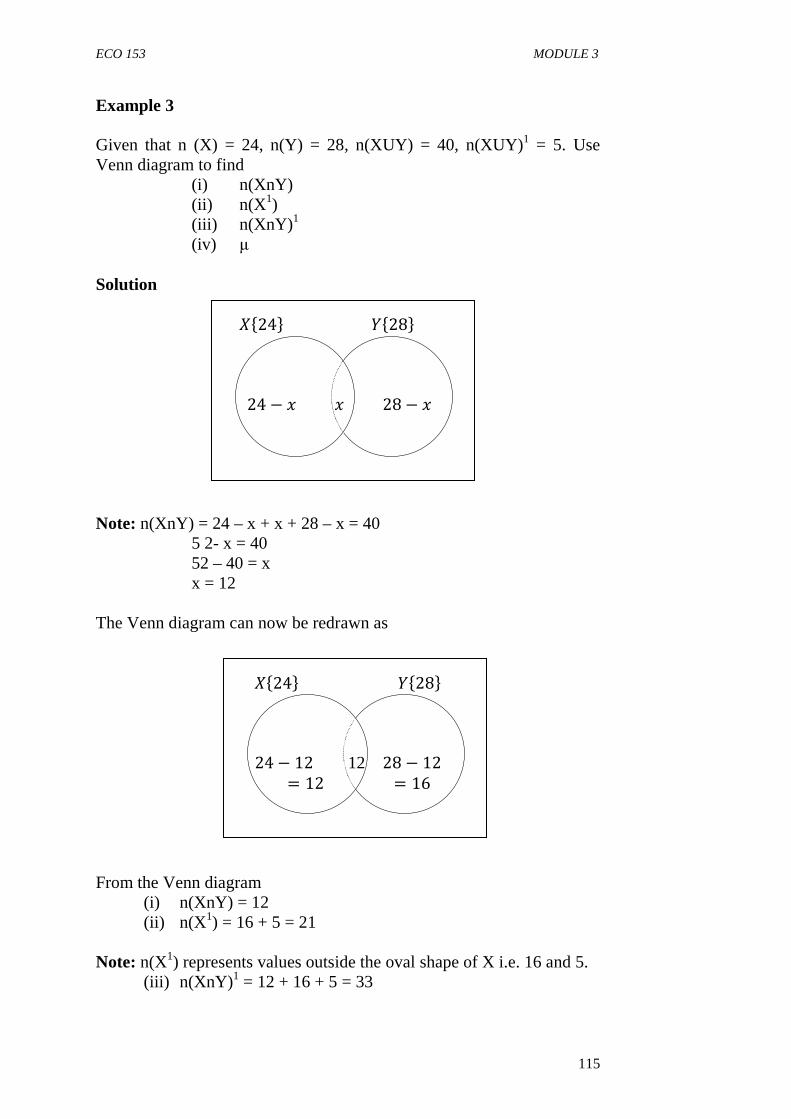
ECO 153 MODULE 3
115
Example 3 Given that n (X) = 24, n(Y) = 28, n(XUY) = 40, n(XUY)1 = 5. Use Venn diagram to find
(i) n(XnY) (ii) n(X1) (iii) n(XnY)1 (iv) µ
Solution ��24���28� 24 − ��28 − �
Note: n(XnY) = 24 – x + x + 28 – x = 40 5 2- x = 40 52 – 40 = x x = 12 The Venn diagram can now be redrawn as ��24���28� 24 − 12 12 28 − 12 = 12 = 16 From the Venn diagram
(i) n(XnY) = 12 (ii) n(X1) = 16 + 5 = 21
Note: n(X1) represents values outside the oval shape of X i.e. 16 and 5.
(iii) n(XnY)1 = 12 + 16 + 5 = 33
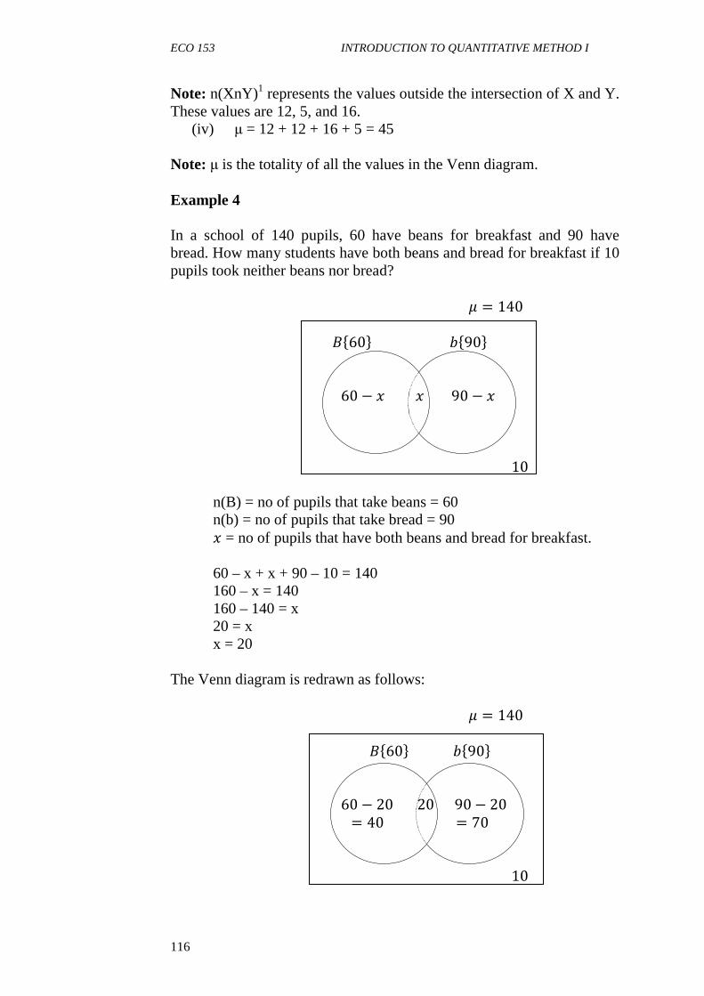
ECO 153 INTRODUCTION TO QUANTITATIVE METHOD I
116
Note: n(XnY)1 represents the values outside the intersection of X and Y. These values are 12, 5, and 16.
(iv) µ = 12 + 12 + 16 + 5 = 45
Note: µ is the totality of all the values in the Venn diagram. Example 4 In a school of 140 pupils, 60 have beans for breakfast and 90 have bread. How many students have both beans and bread for breakfast if 10 pupils took neither beans nor bread? � = 140 ��60� �90� 60 − ��90 − � 10 n(B) = no of pupils that take beans = 60
n(b) = no of pupils that take bread = 90 � = no of pupils that have both beans and bread for breakfast.
60 – x + x + 90 – 10 = 140 160 – x = 140 160 – 140 = x 20 = x x = 20
The Venn diagram is redrawn as follows: � = 140 ��60� �90� 60 − 202090 − 20 = 40 = 70 10

ECO 153 MODULE 3
117
Note: 10 + 40 + 20 + 70 = 140 40 + 20 = 60 20 + 70 = 90
... 20 pupils have both beans and bread for breakfast
Example 5 In a class of 60 students, 30 speak English Language fluently while 25 speak French language fluently. If 5 students can speak both languages, how many cannot speak either of the languages? How many speak only one language?
Solution � = 60 ��30���25� 30 − 5 25 − 5 = 25 = 20 �
n(E) = No of student that speak English language fluently = 30 n(F) = No of student that speak French Language fluently = 25 n(EnF) = no of student that can speak both English Language and
French = 5 x = No of students who cannot speak any of the Languages
... x + 25 + 5 + 20 = 60 x + 50 = 60 x = 60 – 50 x = 10
Therefore, those who speak only one language are those who speak French only and those who
speak English only. = (30 – 5) + (25 - 5) = 25 + 20 = 45
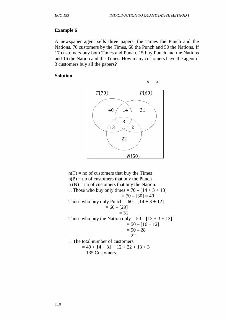
ECO 153 INTRODUCTION TO QUANTITATIVE METHOD I
118
Example 6 A newspaper agent sells three papers, the Times the Punch and the Nations. 70 customers by the Times, 60 the Punch and 50 the Nations. If 17 customers buy both Times and Punch, 15 buy Punch and the Nations and 16 the Nation and the Times. How many customers have the agent if 3 customers buy all the papers? Solution � = � ��70���60�
401431 3 13 12 22
��50� n(T) = no of customers that buy the Times n(P) = no of customers that buy the Punch n (N) = no of customers that buy the Nation. ... Those who buy only times = 70 – [14 + 3 + 13]
= 70 – [30] = 40 Those who buy only Punch = 60 – [14 + 3 + 12]
= 60 – [29] = 31
Those who buy the Nation only = 50 – [13 + 3 + 12] = 50 – [16 + 12] = 50 – 28 = 22
... The total number of customers = 40 + 14 + 31 + 12 + 22 + 13 + 3 = 135 Customers.
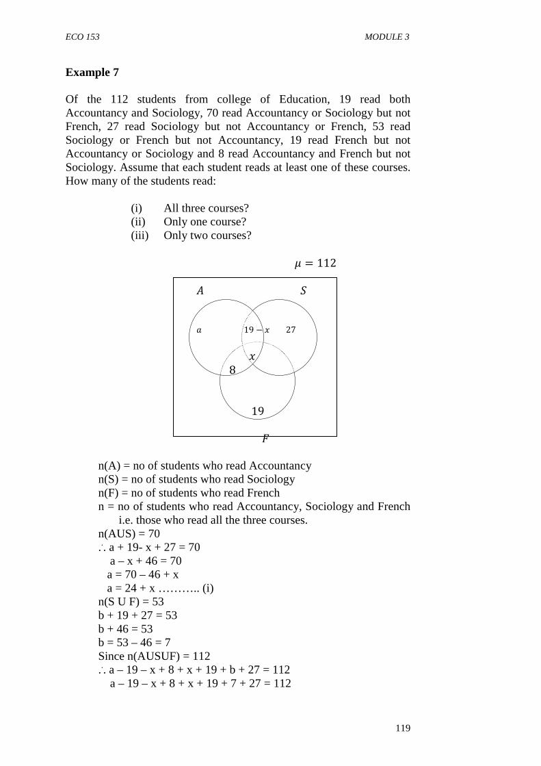
ECO 153 MODULE 3
119
Example 7 Of the 112 students from college of Education, 19 read both Accountancy and Sociology, 70 read Accountancy or Sociology but not French, 27 read Sociology but not Accountancy or French, 53 read Sociology or French but not Accountancy, 19 read French but not Accountancy or Sociology and 8 read Accountancy and French but not Sociology. Assume that each student reads at least one of these courses. How many of the students read:
(i) All three courses? (ii) Only one course? (iii) Only two courses?
� = 112 �� �19 − �27
� 8 19 �
n(A) = no of students who read Accountancy n(S) = no of students who read Sociology n(F) = no of students who read French n = no of students who read Accountancy, Sociology and French
i.e. those who read all the three courses. n(AUS) = 70 ... a + 19- x + 27 = 70 a – x + 46 = 70 a = 70 – 46 + x a = 24 + x ……….. (i) n(S U F) = 53 b + 19 + 27 = 53 b + 46 = 53 b = 53 – 46 = 7 Since n(AUSUF) = 112 ... a – 19 – x + 8 + x + 19 + b + 27 = 112 a – 19 – x + 8 + x + 19 + 7 + 27 = 112
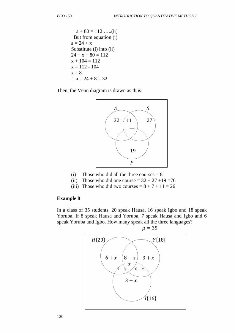
ECO 153 INTRODUCTION TO QUANTITATIVE METHOD I
120
a + 80 = 112 …..(ii) But from equation (i) a = 24 + x Substitute (i) into (ii) 24 + x + 80 = 112 x + 104 = 112 x = 112 - 104 x = 8 ... a = 24 + 8 = 32
Then, the Venn diagram is drawn as thus: �� 321127
19
�
(i) Those who did all the three courses = 8 (ii) Those who did one course = 32 + 27 +19 =76 (iii) Those who did two courses = 8 + 7 + 11 = 26
Example 8 In a class of 35 students, 20 speak Hausa, 16 speak Igbo and 18 speak Yoruba. If 8 speak Hausa and Yoruba, 7 speak Hausa and Igbo and 6 speak Yoruba and Igbo. How many speak all the three languages? � = 35 ��20���18� 6 + �8 − �3 + � � 7 − � 6 − � 3 + �
��16�
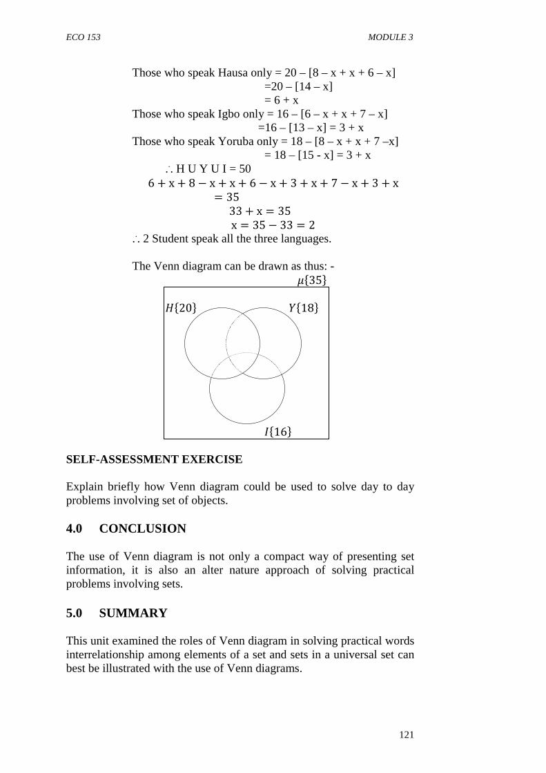
ECO 153 MODULE 3
121
Those who speak Hausa only = 20 – [8 – x + x + 6 – x] =20 – [14 – x] = 6 + x
Those who speak Igbo only = 16 – [6 – x + x + 7 – x] =16 – [13 – x] = 3 + x Those who speak Yoruba only = 18 – [8 – x + x + 7 –x] = 18 – [15 - x] = 3 + x
... H U Y U I = 50 6 + x + 8 − x + x + 6 − x + 3 + x + 7 − x + 3 + x
= 35 33 + x = 35 x = 35 − 33 = 2
... 2 Student speak all the three languages. The Venn diagram can be drawn as thus: -
��35� ��20���18�
��16� SELF-ASSESSMENT EXERCISE Explain briefly how Venn diagram could be used to solve day to day problems involving set of objects. 4.0 CONCLUSION The use of Venn diagram is not only a compact way of presenting set information, it is also an alter nature approach of solving practical problems involving sets. 5.0 SUMMARY This unit examined the roles of Venn diagram in solving practical words interrelationship among elements of a set and sets in a universal set can best be illustrated with the use of Venn diagrams.
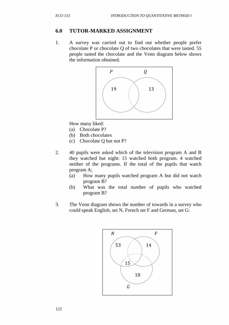
ECO 153 INTRODUCTION TO QUANTITATIVE METHOD I
122
6.0 TUTOR-MARKED ASSIGNMENT 1. A survey was carried out to find out whether people prefer
chocolate P or chocolate Q of two chocolates that were tasted. 55 people tasted the chocolate and the Venn diagram below shows the information obtained.
��
1913
How many liked: (a) Chocolate P? (b) Both chocolates (c) Chocolate Q but not P?
2. 40 pupils were asked which of the television program A and B they watched but night: 15 watched both program. 4 watched neither of the programs. If the total of the pupils that watch program A; (a) How many pupils watched program A but did not watch program B? (b) What was the total number of pupils who watched program B?
3. The Venn diagram shows the number of towards in a survey who could speak English, set N, French set F and German, set G:
�� 53 14
15 18
�
ECO 153 MODULE 3
123
(a) How many tourists altogether were questioned in the survey? (b) How many tourists could speak the following languages?
(i) English and German (ii) Only German (iii) Neither English, French or German
4. In a survey to determine the most popular hotel in Bauchi, Nigeria; some businessmen who come to Bauchi frequently were interviewed and the following results obtained: 60 said they stay in Zaranda 60 Hotel, 75 in Awala and Sogiji Hotels, 54 patronise Zandara and Sogiji. All least interviewed have patronised at least one or the three hotels. If 40 of these businessmen patronised Awala hotel only: (a) How many of them patronise all the three hotels? (b) How many businessmen were interviewed altogether (c) How many patronise Sogiji Hotel only?
5. (a) Given that n(X) = 17, n(Y) = 13 and n (XnY) = 5. Use Venn diagram to find n(XnY)1. If � = 40. (b) If n(X) = 19, n(X) = 20 and n(XUY) = 39. Use Venn diagram to find n(XnY). (c) If n(Y) = 10, n(XUY) = 26 and n(XnY) = 5. Use Venn diagram to find n(X).
7.0 REFERENCES/FURTHER READING Adu, D. B. (1998). Comprehensive Mathematics for Senior Secondary
Schools. Lagos: A. Johnson Publishers. Harwood, C. L. (1990). Ordinary Level Mathematics. (6th ed.). London:
Heinemann Educational Books Limited. Murray, L. (1987). Progress in Mathematics. London: Thornes
Publishers Limited. Usman, A. S. (2005). Business Mathematics. Lagos: Apex Books
Limited.
ECO 153 INTRODUCTION TO QUANTITATIVE METHOD I
124
MODULE 4 SEQUENCE AND SERIES Unit 1 Meaning and Types of Sequence and Series Unit 2 Arithmetic Progression (AP) Unit 3 Geometric Progression (GP) Unit 4 Application of Series and Sequences to Economics, Business and Finance UNIT 1 MEANING AND TYPES OF SEQUENCE AND SERIES CONTENTS 1.0 Introduction 2.0 Objectives 3.0 Main Content 3.1 General Overview 3.2 Definition and Types of Sequence and Series 4.0 Conclusion 5.0 Summary 6.0 Tutor-Marked Assignment 7.0 References/Further Reading 1.0 INTRODUCTION In the first module of this book, you were introduced to the real number system. You will observe that integers are set of negative and positive whole numbers including zero (0) as a neutral number. A set of integer may be written following a particular order e.g. (a) 1, 2, 3, 4, 5 …………… …………. (b) - 1 - 2 - 3 - 4 - 5 - 6 - 7 ……………… (c) 2, 4, 6, 8, 10, 12 ……………………. (d) 1, 4, 9, 16, 25, 36 ……………… (e) - 10, - 20, - 30, - 40, - 50, - 60, -70 ……………. (f) 2, 4, 8, 16, 32, 64, 128 ………………….. You observe that each of these set of number has its own peculiar pattern or order of construction. For example, (a) Is a set of positive integer (increasing by a unit i.e. adding (1) one
to the previous) (b) Is a set of negative integers (reducing by a unit i.e. subtracting (1)
from the previous

ECO 153 MODULE 4
125
(c) Is a set of positive even numbers (obtained by continuous addition of 2)
(d) Is set of squares of numbers i.e. perfect squares (e) Is obtained by subtracting 10 from the subsequent set of numbers (f) Is obtained by multiply the subsequent term by 2 These set of numbers are written based on a specific rule and they are collectively known as sequence. It should be noted that sequence can also be a set of fractions, decimals or even indices. The essential requirement for a set of number to form a sequence is that there must be a defined pattern or rule(s) in forming the set of numbers or terms. 2.0 OBJECTIVES At the end of this unit, you should be able to: • define the term “sequence” and “series” • identify the basis types of sequence series • solve problem involving arithmetic progression and geometric
progression • apply the basic principles of sequence and series to solve practical question relating to sequence and series. 3.0 MAIN CONTENT 3.1 General overview Every magnitude (figure) has the tendency to increase, decrease, be multiplied or remain constant over time. The ability of a positive number to increase is subject to be added to another positive number (except 1). Similarly, a positive number decrease when it is added to another negative number or a positive number is taken from it or divided by a positive number (except 1). A number remains the same if multiplied by 1, divided by 1 or added to zero or zero subtracted from it. A sequence is formed when a set of number is increasing or decreasing by a constant value as the term of the sequences are being formed. For example: a. -2,-4,-6,-8,-10, ................ b. 4, 8, 10, 11, 15, 17, 19, …. c. 10, 20, 30, 40, 50, 60, …… d. 2, 6, 8, 54, 162, ……….…. e. 90, 80, 75, 65, 50, 40, …..
ECO 153 INTRODUCTION TO QUANTITATIVE METHOD I
126
It should be noted that only sets of numbers in (a), (b) and (d) form sequence of number because the pattern of the decrease or increase is uniform over time. Although set of increases but not by a constant value, so also the set of numbers in (e). Therefore set of numbers in (a), (c) and (d) form a sequence, while those in (b) and (e) do not. SELF-ASSESMENT EXERCISE For each of the following set of number, state whether it is a sequence or not. i. 10, 9, 8, 7……......... ii. 8, 9, 11, 14, 18, 23………… iii. 0, -2, -4, -6, -8………… iv. 144, 72, 36, 18………... v. 1/144,
2/121, /100, 4/81,
5/64………… 3.2 Definition and Types of Sequence and Series A sequence or progression of numbers is a set of number arranged in some order or rules with a constant pattern of growth or decline in the set of figures which will guide us to determine successive terms from their predecessors. Example of see include: 2, 4, 6, 8, 10, ………….. 2, -1, -4, -7, -10, ………….. 1, 2, 4, 8, 16, 32, ………….. It could be observed that in the first sequence, each successive term is greater than its predecessor by 2. In the second sequence each successive term is smaller than its predecessor by 3 while in the third sequences each successive term is twice its predecessor. A series is obtained when the terms of the sequence are connected by positive or negative signs e.g. 2 + 4 + 6 + 8 + 10… 2 + (-1) + (-4) + (-7) + (-10)… 144 – 72 – 36 -18 …. A series in which successive terms have a common different or common ratio known as progressive. These are two major types of progressive namely: i. Arithmetic progression ii. Geometric progression A sequence or progression of numbers where terms have constant difference is arithmetic sequence or progressive.
ECO 153 MODULE 4
127
The sum of the terms is called arithmetic series. This implies that if a sequence of the term (set of numbers) is such that the different between any terms and the one immediately preceding it is a constant, such terms are said to form arithmetic progression. Examples of the arithmetic progression are: 5, 8, 11, 14… 3, -1, -5, -9…… -2, -3\ 4, 1\2, 13\4 ….. a, a + d, a + 2d, a + 3d … a – 2d, a – d, d, a+ d, a + 2d …. An arithmetic progression is therefore described as a progression or series formed by continuous addition or subtract of a constant value called the "common difference” (d). In the example above, the common different of 5, 8, 11, 14… is 3 , that of 3 , - 1 , -5 , - 9 , is – 4 , the
common different of −2, ���, �
�, 1, 1 �
�……….is 1 �
� while that of at a –
2d, a- d, a, a + d… is d. The common difference can be obtained as thus: T2 –T1 = T3 – T2 = T4 – T3……Tn – (Tn – 1) Where T2 = second term, T3 = third term, T1 = first term, T4 = fourth term, Tn = nth term and Tn-1 is the term that preceded the nth term. If, in a sequence of terms, each term is a constant multiple of the preceding the terms are said to be in geometric progression. In a geometric progression (or sequence), there is a common ratio between each term and the previous term. The sum of the term in such progression is known as geometric series. A geometric progression has the same ratio of all consecutive terms. It can also be defined as a sequence which is formed by a continuous multiplication or division by a constant value known as a common ratio (r). The common ratio (r) is
given as 1
2
T
T
= 2
3
T
T
= 3
4
T
T
=…………. 1−n
n
T
T
where T1,T2, T3, T4, and Tn - 1 are as defined under the geometric progression. Examples of geometric progression (GP) are: 3, 6, 12, 24 ….. 8, 4, 2, 1, ½ ……. 2 – 10, 50 ……. a, ar, ar2, ar3 …… In the first example successive terms obtained by multiplying to
preceding term by 2 (the common rate is 3
6
= 2). In the second example,

ECO 153 INTRODUCTION TO QUANTITATIVE METHOD I
128
the successive terms are obtained by multiply the preceding term by 21
or by dividing the preceding term by 2 (the common ratio is =
8
4
2
1
). In
the third example, common ratio ==
a
ar
ar
ar 2
= r It should be noted that a special sequence or progression is obtained by certain manipulation that is not uniform. Successive terms are obtained by reasoning and following the trend or pattern of the sequence. Such sequences are not generated by a specific formula. Example includes: 1, 4, 9, 16, 25….........
,121
1
100
2,81
3
,64
4
,49
5
………….. 8, 9, 1, 14, 18, 23 ………….. The first sequence is a set of perfect square i.e. square of numbers. You will observe that the differences between each of the successive terms is not constant (the first is 3, then 5, then 7, then 9) but the difference themselves form an arithmetic progression. The second example is a sequence obtained by fraction of increasing whole number numerators and decreasing perfect square denominator. Although, other terms in the sequence can be generated but by general reasoning. The last example under the special sequence is obtained by an increasing difference. The difference between 8 and 9 is 1 that of 9 and 11 is 2, and so on. Hence, the differences, not the term form the AP of 1, 2, 3, 4, 5………. SELF-ASSESSMENT EXERCISE i. Distinguish clearly between arithmetic progression and geometric
progression. Give example of each. ii. In what ways is special sequence different from arithmetic
progression and geometric progression? 4.0 CONCLUSION Progression or sequence are not just sets of increasing or decreasing numbers but a set of numbers formed following a defined rule. This makes it difference from special sequence which are formed by manipulations obtainable from the trend or pattern of the existing terms.

ECO 153 MODULE 4
129
5.0 SUMMARY Sequence can broadly be classified into two; arithmetic progressions (formed by continuous addition or subtraction of a common difference) and the geometric progression (formed by a continuous multiplication or division by a common difference). At the extreme are the special sequences which are generated by aptitude reasoning. 6.0 TUTOR-MARKED ASSIGNMENT For each of the following progression, 1. Identity the type of sequence 2. State the common difference or the common ratio (if it is AP or
GP) 3. Generate the next four terms of the sequence:
(i) 1, 2, 3, 4, 5 ……………. (ii) 1, 4, 9, 16, 25 ………….. (iii) 8, 9, 11, 14, 18, 23 …………. (iv) 6, 4, 2, 0, -2 …………. (v) 144, 72, 36, 18 …………….. (vi) 2, 4, 8, 16, 32 …………….
(vii) 1441
, 1212
, 1003
, 814
…………………..
(viii) 101
, 94
, 89
, 716
, 625
, 536
……………. 7.0 REFERENCES/FURTHER READING Hardwood, C. L. (1978).Ordinary Level Mathematics. (6th ed.).
London: Heinemann Educational Books. Robert, S. & Geoff, B. (2007). Excellence in Mathematics for Senior
Secondary Schools. Lagos: Macmillan Publishers Limited. Usman, A. S. (2005). Business Mathematics. Lagos: Apex Books
Limited.
ECO 153 INTRODUCTION TO QUANTITATIVE METHOD I
130
UNIT 2 ARITHMETIC PROGRESSION CONTENTS 1.0 Introduction 2.0 Objectives 3.0 Main Content 3.1 nth Term of Arithmetic Progression 3.2 Sum of Arithmetic Progression 4.0 Conclusion 5.0 Summary 6.0 Tutor-Marked Assignment 7.0 References/Further Reading 1.0 INTRODUCTION In the preceding unit, you have learnt about two major types of sequence namely, arithmetic progression (AP) and the geometric progression (GP). You are aware that arithmetic progressions are generated by a continuous addition of a common difference and that the pattern can continue over a set of terms. Some mathematical formula can be used to generate large numbers of terms. Manual generation of such terms by following the rules may be time consuming and hectic when some terms such as 50th terms, 100th term, etc. are to be generated. More so, sum of terms no matter how large the number of terms is, can be obtained using some mathematical formula. The formula generating the term is called the nth term formula while the one generating the sum is the sum of the arithmetic progression to the nth term. 2.0 OBJECTIVES At the end of this unit, you should be able to: • generate the nth tern of the progression • generate the sum of a given arithmetic progression • obtain the common difference or the first term of an AP given
some sets of information.
ECO 153 MODULE 4
131
3.0 MAIN CONTENT 3.1 nth Term of Arithmetic Progression The nth term of an arithmetic progression (AP) is the mathematical formula used to generate any term in a given arithmetic progression. Assuming the first term of an AP is given as ‘a’ and the common difference is given as ‘d’. Then the nth term of an AP is mathematically given as: Tn= a + (n - 1)d, where Tnis the nth term. For instance, 4th term = T4 = a + (4 - 1)d = a + 3d 18th term = T18 = a + (18 -1)d = a + 17d, and so on. Examples 1. Find 127th term of the AP given as 5, 8, 11…. Solution Tn = a+ (n-1)d a = 1st term = 5 d = common difference = T2 – T1 = 8 – 5 = 3 T127 = a + (127-1) 3 T127 = 5 = (126) 3 T127 = 5 + 378 T127 = 383 2. How many term has the arithmetic progression 8, 11, 14, 17, …, 380 Solution Note: Tn= a + (n - 1)d The question requires the position of 380 in the arithmetic progression i.e. the value of n, given that Tn = 380, a = 8 and d = 11- 8 = 3 380 = 8 + (n – 1)3 380 = 8 + 3n – 3 380 – 8 + 3 = 3n 372 + 3 = 3n
n = 3
375
= 125 Therefore the AP has 125 terms.
ECO 153 INTRODUCTION TO QUANTITATIVE METHOD I
132
3. Insert 6 arithmetic terms between -3 and 18. Solution Let the AP be -3, a, c, d, e, f, g, 18 i.e.b, c, d, e, f, and g are the terms to be inserted. Tn = a + (n – 1)d 18 = -3 + (8 – 1)d Note: 18 now becomes the 8th term and the difference is not yet known. Opening the brackets, we have 18 = -3 + 7d 18 + 3 = 7d 21 = 7d
d = 7
21
d = 3 Since the difference = 3 and a = -3 b = 2nd term = a + d = -3 + (-3) = 0 c = 3rd term = a + 2d = -3 + 2(3) = 3 d = 4th term = a + 3d = -3 + 3(3) = 6 e = 5th term = a + 4d = -3 + 4(3) = 9 f = 6th term = a + 5d = -3 + 5(3) = 12 g = 7th term = a + 6d = -3 + 6(3) = 15 Hence, the terms inserted are b, c, d, e, f, and g which are 0, 3, 6, 9, 12, 15, Then the AP becomes: 0, 3, 6, 9, 12, 15, 18. 4. The 21st term of an AP is 50,000, if the first term is 20,000. Find the common difference. Solution Tn = a + (n – 1) d 50000 = 20,000 + (21 – 1)d 50,000 = 20,000 + 20d 50,000 – 20,000 = 20d 30 000 = 20d d = 30,000 = 1500 20 5. The fifth and eighth term of an AP are 9 and 27 respectively. Find (a) The common difference; (b) The first term; (c) The nth term; and (e) The 21st term.
ECO 153 MODULE 4
133
Solution Tn = a + (n – 1) d T5 = a + (5 – 1) d 9 = a + 4d - -- - - - (i) Likewise, T8 = a + (8-1)d 27 = a + 7d -------- (ii) Solving (i) and (ii) simultaneously, - a + 4d = 9 ……… (i) a + 7d = 27 ………. (ii), subtracting (i) from (ii) 7d – 4d = 27 – 9 3d = 18 d = 18/3
d = 6 ... Common difference = 6 From equation (i) 9 = a + 4d 9 = a + 4(6) 9 = a + 24 9 - 24 = a a = -15 The AP is -15, (-15 + 6), (-15 + 6 + 6), (-15 + 6 + 6 + 6)……….. = -15, -9, -3, 3, 9, 15, 21, 27 The nth term if the AP, Tn= a + (n – 1)d = -15 + (n – 1) d -15 + (n – 1) 6 -15 + 6n – 6 = -21 + 6n. :. 21st term = T21 = a + (21 – 1)d T21 = -15 + (20)d T21= - 15 + 20(6) T21 = -15 +120 =105 SELF-ASSESSMENT EXERCISE i. Find the 10th term of the following AP (a) 1, 4, 7 …….. (b) 2, 21/2, 3 …… (c) 10, 8, 6 …….. ii. The 4th term of an AP is 13 and the second term is 3 find the
common different and the first term iii. The 4th and the 7th term of an arithmetic sequence are 6 and 15
respectively. Find the nth term of the sequence

ECO 153 INTRODUCTION TO QUANTITATIVE METHOD I
134
iv. The 9th term of an arithmetic sequence is 12 and the 17th term is 28. Find the 4th term.
v. If 3, x, y, 18 are in AP. Find x and y 3.2 Sum of an Arithmetic Progression Term in an arithmetic progression can be added together using either of the formula below.
Sn ={ }la
n+
2 where a = first term and l = Last term n = nth term. i.e. the number of terms to be added .
OR
Sn= { }dna
n)1(2
2−+
where a = first term d = common different and n = nth term. The two formulae are proved the same as thus: Recall, AP is in the form: a, a + d, a + 2d……….. Therefore, their sums become a + (a + d) + (a + 2d) +………….. (i) Recall that the nth term = a + (n – 1)d, call this l. Writing the series from backward we have l + (l - d) + (l - 2d) …….. ………. (ii) Each term of series in (i) added to the corresponding term of series in (ii) gives (a + l). There are n terms and so the sum is n(a + l).This is the
sum of two equal series and so the sum of each is )(
2
1lan +
Recall that l = ( )dna 1−+
And so
{ }{ }{ }dna
nor
dnan
dnaanlan
)1(22
)1(22
1
)1(2
1)(
2
1
−+
−+=
−++=+
ECO 153 MODULE 4
135
Example 1. Find the sum of 28 term of the arithmetic progression 3 + 10 + 17 +…… Solution
a = 3, d = 7, n = 28, Sn ={ }dna
n)1(2
2−+
S28=
{ }{ } { } 2730)19514)7(27614
7)128(322
28
==+=
−+×
2. An arithmetic sequence has first term as 3 and the common difference of 2. How many terms are needed to make sum equal to 99? Solution
Recall: Sn ={ }dna
n)1(2
2−+
Sn = 99, n = unknown, a = 3, d = 2
: 99 = { }2)1(32
2
1−+× nn
99 =
{ }2262
1−+ nn
, cross multiply
198 = { }226 −+ nn
198 = { }nn 24+ 198 = 4n + 2n2 ... 2n2 + 4n – 198 = 0 (divide through by 2) n2 + 2n – 99 = 0 Using factorisation method, n2 + 11n – 9n – 99 =0 n(n +11) -9 (n +11) =0 (n – 9) (n + 11) = 0 n - 9 = 0 n = 9 or n + 11 = 0, n = - 11 Therefore 9 terms are needed to make sum equal to 99. 3. Find the sum of the AP given as: 1 + 31/2 + 6 + ……. + 101 Solution a = 1 d = 31/2-1=21/2 or 2.5 nth term =101 ... nth term = a + (n - 1)d
ECO 153 INTRODUCTION TO QUANTITATIVE METHOD I
136
101 = 1 + (n -1)2.5 101 = 1 +2.5n - 2.5 101 – 1 +2.5 = 2.5n 102.5 = 2.5n N = 102.5 2.5 n = 41 : The AP has 41 terms
: Sum of AP = Sn ={ }dna
n)1(2
2−+
S41 = { }5.2)141(12
2
41−+x
S41 = 20.5{ }5.2402 x+
= 20.5 { }1002+
= 20.5 { }102 = 2091 4. The first and the last term of an AP are 5 and 100 respectively. Find the sum of the AP, if the AP has 20 terms. Solution
{ }la
nSn +=
2
{ }1005
2
2020 +=S
=20S 10 { }105 = 1050. SELF-ASSESMENT EXERCISE i. Find the sum of the first 14 term of the AP. 2 + 5 + 8 + 11 + 14
+ 17 +….. ii. The 7th term of an arithmetic sequence is 12 and the 11th term is -
3. Find the sum of the first three terms. iii. The second term of an arithmetic sequence is 15 and the sum of
40th term is 3560. Find the sum of the first 41 terms. iv. How many term of the series 2 + 5 + 8 + 11+……are needed for
the sum to exceed 200? v. Find the sum of the 18 term of the series 21/2 + 33/4+5+…. vi. Find the sum of the AP given as 30…….. 720 if there are 50 term
in the AP.
ECO 153 MODULE 4
137
4.0 CONCLUSION Series are obtained when term of a sequence are connected with positive or negative signs e.g. 2 + 4 + 6 + 8 + 10, 2 – 1 – 4 – 7 - 10.or 2 + (-1) + (-4) +(-7) + (-10)……. Sometimes the term may be so numerous that mental summing up of the term may be extremely difficult. In such circumstance the formula for finding the sum of arithmetic progression (AP) is applied. 5.0 SUMMARY Sum of arithmetic can be obtained using two approaches depending on the nature of arithmetic progression.
The sum of AP = Sn ={ }dna
n)1(
2−+
, when the common difference can be obtained, however, when only the first term and the last terms are
given the sum of the AP is given as Sn ={ }la
n+
2 . Two formulas have been proved to be the same. 6.0 TUTOR-MARKED ASSIGNMENT 1. An arithmetic sequence has its first term as 2 and the common difference 3 the sum of the nthterm is 77. Find n. 2. The first term of an arithmetic sequence is 8 and the sum of the first 20 terms is 445. Find the common difference 3. The third term of an Arithmetic Progression is 8 and the 16th term is 47. Find the first term and the common difference of this AP. 4. The 14th term of an AP is -15 and the common difference is -5. Find the first term and write the first six terms. 5. If -5, p, q, 16 are in AP. Find p and q. 6. Find n, given that 697 is the nth term of the AP.4, 11, 18….. 7. How many terms have the series 1, 4, 7 …….(6n – 2)? 8. The sum of the 3rd and 9th term of an AP is 6 and their product is 8. Find the sum of the first fifteen term of the sequence. 9. Given that 3 + 7 + 11 + 15 +…. is an AP find a. the nth term; b. the 11th term (T11); and c. the sum of the first 120 natural numbers divisible by 6.
ECO 153 INTRODUCTION TO QUANTITATIVE METHOD I
138
7.0 REFERENCES/FURTHER READING Hardwood, C. L. (1978). Ordinary Level Mathematics. (6th ed.).
London: Heinemann Educational Books Limited. Koop, J. S. (1990). Mathematics for Business. US: Win C. Brown
Publishers. Selah, U. A. (2003). Quantitative Techniques in Business. Maiduguri:
Compaq Publishers.
ECO 153 MODULE 4
139
UNIT 3 GEOMETRIC PROGRESSION CONTENTS 1.0 Introduction 2.0 Objectives 3.0 Main Content 3.1 nth Term of Geometric Progression 3.2 Sum of Geometric Progression 4.0 Conclusion 5.0 Summary 6.0 Tutor-Marked Assignment 7.0 References/Further Reading 1.0 INTRODUCTION In the last unit, you learnt about arithmetic progression which is a sequence of numbers generated by continuous addition or subtraction of a constant number called common difference. Sequences are of two main types namely arithmetic progression and geometric progression. Geometric progression unlike the arithmetic progression, are sequence of numbers generated by continuous multiplication or division by a constant value called the common ratio. Some mathematical formula can be used to generate large volume of term of geometric progression. Geometric progression have the tendency to generate extremely large or small numbers such that it could be extremely taskful and time consuming to obtain terms like 50th term, 100th term, etc. More importantly, sum of geometric progression, no matter the quantity of the term being considered can be easily obtained with the use of mathematic formulas depending on size of the common ratio the formulas generating the terms in the geometric progression is called the nth term of the GP while the one used to compute the sum of the GP is the sum of GP to the nth term. 2.0 OBJECTIVES At the end of this unit, you should be able to: • generate the nth term of geometric progression • generate the sum of any given geometric progression • obtain the common ratio or the first term of a GP, provided some
adequate information are given.

ECO 153 INTRODUCTION TO QUANTITATIVE METHOD I
140
3.0 MAIN CONTENT 3.1 nth Term of Geometric Progression The nth term of a geometric progression (GP) is the mathematical formula used to generate any term in a given geometric progression. Assuming the first term of a GP is ‘a’ and the common ratio is ‘r’ then the nth term of a GP = Tn= arn-1, where Tn is the nth term e.g. 6th term = T6 = ar6-1 = ar5 12th term =T12 = ar12-1 = ar11, and so on. Example 1. Given a series as follow 2 + 4 + 8 + 16 + …. Find the value of the 20th term of the sequence. Solution The sequence is a GP because the proceeding term is being multiplied by a constant value. To generate the subsequent terms. Tn= arn-1
T20 = arn-1, r = 1
2
T
T
= 2
2
4=
T20 = 2 (2)20-1 =21. 219 = 220 2. Insert four geometric terms between 2 and 486. Solution Let the GP be: 2, w, x, y, z. 486. Therefore 486 becomes the 6th term. ... T6 = arn-1 T6 = ar6-1 486 = ar5 486 = 2r5 Divide both sides by 2 243 = r5
r = 32435=
w = 2 x r = 2 x 3 = 6 x = 6 x r = 6 x 3 = 18 y = 18 x r = 18 x 3 = 54 z = 54 x r = 54 x r = 162. Therefore, the four terms inserted in the GP are 6, 18, 54, and 162.
ECO 153 MODULE 4
141
1. The 6th and 9th term of a GP are 96 and 768 respectively. Find i. The common ratio; ii. The first term; and iii. The nth term. Solution T6 = ar6-1 : 96 = ar5……… (i) Ta = ar9-1 : 768 = ar8 ….. (ii) Solving (i) and (ii) simultaneously: ar5 = 96 ………… (i) ar8 =768………… (ii), dividing (ii) by (i)
96
768
5
8=
ar
ar
85
8 =rr
r8-5= 8 r3 = 8
r = 283=
From equation (i), ar5=96 a(2)5 = 96 a(32) = 96 32a = 96 Dividing both side by 32
32
96
32
32=
a
a = 3 The nth term = arn-1 = 3(2)n-1
SELF-ASSESMENT EXERCISE i. Insert 2 geometric terms between 7 and 189 ii. If the 3rd and the 6th term of and GP are 18 and 486 respectively.
Find the common ratio, the first term and the10th term iii. Find the 9th term of the GP: 40, 20, 10 … iv. The third term of a geometric sequence is 36 and the sixth term is
121.5. Find the first four terms of the sequence v. The second term of a geometric progression is 6 and the fifth
term is 162. Find the third term vi. Find the sixth term of the following GPs (a) 3, 6, 12…. (b) -4, 2, -1 …
(c) 3, 2, 34
vii. Find the 40th term of the GP 2, 14, 98…. viii. Find n given that 1024 is the nth term of the GP 4, 8, 16….
ECO 153 INTRODUCTION TO QUANTITATIVE METHOD I
142
ix. If 5, x, y, 40 are in GP. Find x and y x. Find the geometric mean of 35 and 140 (hint geometric mean of x
and y = xy . 3.2 Sum of Geometric Progression Suppose S denotes the sum of n terms of the GP, whose first is a and common ratio = r, then S = a + ar + ar2 + ar3 + …. + arn-2 + arn-1
………….. (1) Multiplying both sides by r. R = ar + ar2 + ar3 + ……. + arn -1 + arn ………………... (2) Subtracting (ii) form (i) S – rs = a – arn S (1 – r) = a (1 – rn) ( )
r
raS
n
−
−=
1
1
, this is applicable when r < 1 (both numerator and denominator of the fraction are positive and this is the most convenient form of S. if however, r > 1 Then S = a (rn-1) r -1 Note: The sum of GP to infinity is given as
r
aS
−=∞ 1 this is more applicable when r < 1
Examples 1. Find the sum of eight terms of the GP 2, 6, 18 ……. Solution Sn = a (rn – 1), a = 2, r = 6/2 = 3 r -1 S8 = 2[38 -1] = 38 - 1 = 6560 2 2. Find the sum of infinity of series: 2 + (-1) + (1/2) + (-1/4) + (1/8) …. Solution a =
����
= - ½
Sum of GP to infinity = r
aS
−=∞ 1
2 = 2 =2 ÷ 1½ = 2 ÷ 3/2 1 – (- ½) 1 + ½ = 2 x 2/3 = 4/3

ECO 153 MODULE 4
143
3. Given the G.P: 144, 72, 36, 18 …….. Find the sum of the first eight terms Solution
S8 = �(����)
���,r = 2
1
144
72
1
2==
T
T
S8 = 144 (1 – (1/2)8)
1 – 1/2 S8 = 144 (1 – 1/256) 1/2 S8 = 144 (255/256) 1/2 S8 = 144 x 255 x 2 . 256 1 S8 = 2295 8 SELF-ASSESSMENT EXERCISE i. Find the sum of the first nine terms of the Geometrical
Progression below: a. 5 + 10 + 20 + 40 + b. 2 + 4 + 8 + 16 +….. ii. Find the sum of the first 10 terms of the series 1 + 2 + 4 + 8 +…..
How many terms of the series are needed for the sum to exceed 2000?
iii. The first term of a geometric sequence is 64, and the common ratio is -1/4. Find the sum of the first five terms.
iv. Find the sum to infinity of the following series:- a. 2 + 1 + ½ + ¼ +…… b. 3 – 1+ 1/3 – 1/9 + ……
4.0 CONCLUSION The nth term of a geometric progressions and the sum of geometric progressions enable us to generate any term in a GP as well as find the sum of GP with ease. 5.0 SUMMARY The nth term of a GP is given as Tn = arn-1, while the sum of a GP is given as Sn = a(1 -rn) where r <1 1 – r orSn= a (rn -1) where r > 1
ECO 153 INTRODUCTION TO QUANTITATIVE METHOD I
144
r -1 However, the sum of GP to infinity is given as S∞ = a where r < 1
1 - r 6.0 TUTOR-MARKED ASSIGNMENT 1. The third term of a geometric progression is 5, and the fifth term
is 20. Find the possible values of the second term. 2. The third term of a geometric progression is 36 and the sixth term
is 121.5. Find the common difference and the first term 3. Find the value of the 20th term and the sum to the 8th term for the
sequence: 2, 4, 8, 16, 32…. 4. The 5th and the 8th term of an arithmetic progression is 9 and 27
respectively. Find a. The common difference b. The first term c. The AP d. The sum of the AP to the 20th term
5. Find four geometric terms between 2 and 486 6. lf the 3rd and 6th term of a GP are 18 and 486 respectively. Find
the GP the 10th term and the sum of the first ten terms. 7. Find the T10 and S20 for each of the following sequence
(a) -3, 6, -12 (b) -2, -4, 8
8. Find the value of n given that -49 is the nth term of the AP: 11, 8, 5…
9. Find the sum of the first 50 odd numbers 10. Find the nth term of the GP: x, 2xy, 4xy2
7.0 REFERENCES/FURTHER READING Hardwood, C. L. (1978). Ordinary Level Mathematics. (6th ed.).
London: Heinemann Educational Books Limited. Selah, U. A. (2003). Quantitative: Technique in Business. Maiduguri:
Compaq Publishers. Robert, S. & Geoff, B. (2007). Excellence in Mathematics for Senior
Secondary Schools Book 3. Ibadan: Macmillan Publishers.

ECO 153 MODULE 4
145
UNIT 4 APPLICATION OF SEQUENCE AND SERIES TO ECONOMICS, BUSINESS AND FINANCE CONTENTS 1.0 Introduction 2.0 Objectives 3.0 Main Content 3.1 Application of Arithmetic Progression to Economics, Business and Finance 3.2 Application of Geometric Progression to Economics, Business and Finance 4.0 Conclusion 5.0 Summary 6.0 Tutor-Marked Assignment 7.0 References/Further Reading 1.0 INTRODUCTION The purpose of studying mathematical techniques and principles of mathematics in economics and related disciplines is not only to know them but to apply them solve some problems relating to economics business and finance. You will recall that, after studying the basic principles and laws in set theory, we concluded the topic by applying the principles and law to day to day problems. In a similar manner, the basic formulae and principles learnt in sequence and series are not meant to solve mathematical and quantitative problems only, we should be able to adopt these tools in solving practical problems especially those that have to do with economics, business and finances. It is only when this is done, that we can really appreciate the mathematical formulae. 2.0 OBJECTIVES At the end of this unit, you should be able to: • apply basic principles and formulae of arithmetic progression to
solve day to day economics and business related problems • solve practical problems in economics and business using the
basic principles and formulae of geometric progression.
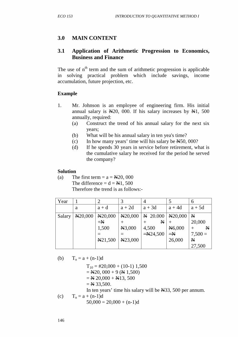
ECO 153 INTRODUCTION TO QUANTITATIVE METHOD I
146
3.0 MAIN CONTENT 3.1 Application of Arithmetic Progression to Economics,
Business and Finance The use of nth term and the sum of arithmetic progression is applicable in solving practical problem which include savings, income accumulation, future projection, etc. Example 1. Mr. Johnson is an employee of engineering firm. His initial annual salary is N20, 000. If his salary increases by N1, 500 annually, required:
(a) Construct the trend of his annual salary for the next six years; (b) What will be his annual salary in ten yea's time? (c) In how many years’ time will his salary be N50, 000? (d) If he spends 30 years in service before retirement, what is the cumulative salary he received for the period he served the company?
Solution (a) The first term = a = N20, 000 The difference = d = N1, 500 Therefore the trend is as follows:- Year 1 2 3 4 5 6 a a + d a + 2d a + 3d a + 4d a + 5d
Salary N20,000 N20,000 +N 1,500 = N21,500
N20,000 + N3,000 = N23,000
N 20.000 + N 4,500 =N24,500
N20,000 + N6,000 =N 26,000
N 20,000 + N 7,500 = N 27,500
(b) Tn = a + (n-1)d
T10 = #20,000 + (10-1) 1,500 = N20, 000 + 9 (N 1,500) = N 20,000 + N13, 500 = N 33,500. In ten years’ time his salary will be N33, 500 per annum. (c) Tn = a + (n-1)d 50,000 = 20,000 + (n-1)d
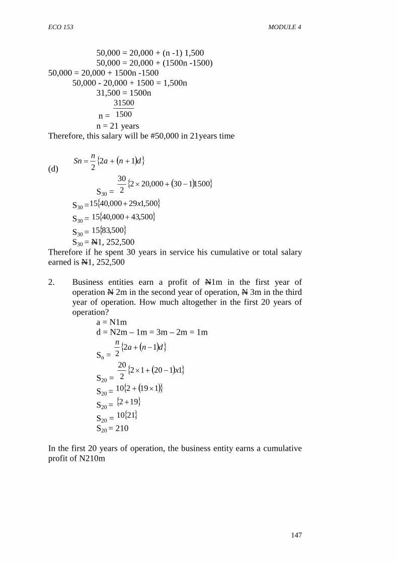
ECO 153 MODULE 4
147
50,000 = 20,000 + (n -1) 1,500 50,000 = 20,000 + (1500n -1500) 50,000 = 20,000 + 1500n -1500 50,000 - 20,000 + 1500 = 1,500n 31,500 = 1500n
n = 1500
31500
n = 21 years Therefore, this salary will be #50,000 in 21years time
(d) ( ){ }dna
nSn 12
2++=
S30 = ( ){ }1500130000,202
2
30−+×
S30 = { }500,129000,4015 x+
S30 = { }500,43000,4015 +
S30 = { }500,8315 S30 = N1, 252,500 Therefore if he spent 30 years in service his cumulative or total salary earned is N1, 252,500 2. Business entities earn a profit of N1m in the first year of
operation N 2m in the second year of operation, N 3m in the third year of operation. How much altogether in the first 20 years of operation?
a = N1m d = N2m – 1m = 3m – 2m = 1m
Sn = ( ){ }dna
n12
2−+
S20 = ( ){ }112012
2
20x−+×
S20 = ( ){ }119210 ×+
S20 = { }192+
S20 = { }2110 S20 = 210 In the first 20 years of operation, the business entity earns a cumulative profit of N210m
ECO 153 INTRODUCTION TO QUANTITATIVE METHOD I
148
SELF-ASSESSMENT EXERCISE i. Aminat starts a job at an annual salary of N600, 000. Every year
she receives a pay rise of 50,000. What is the total amount she has earned in 8 years?
ii. Chiamaka started a job saved N40, 000 in her first year. For each year, she was able to saveN10, 000 more than in the pronoun year. How many years will it take her to save a total ofN600,000?
iii. A man saves N1000 in the first month and increases the savings by N200 each month. What amount does he save by the fourteenth month?
3.2 Application of Geometrical Progression to Economics,
Business and Finances The nth term of a geometric progression and the sum of geometric series is found applicable to a number of areas in economics, finance and business. Among the common application of GP are compound interest, present value, growth rate estimations etc. Examples 1. A student borrows 600 at 7% interest compounded annually. He
pays off the loan at end of 3 years. How much does he pay? Solution 7% of N 600 = N42 2nd term of the GP is N600 + N42 = N642 Hence the GP is 600 + 642+…. a = 600
r = 07.1
600
642=
At the end of the 3rd year the GP will have 4 terms; 4th term = ar3 600 (1.07)3 = 600 (1.2250) = N735 ∴He pays back N735 2. Olawale saved N30, 000 in the first year of a new job. In each
subsequent year, he saved 10% more than in the previous year. a. How much in total had he saved in 5 years? b. How many years did he take to save a total of more than N330, 000?
ECO 153 MODULE 4
149
Solution
a. a = N30,000
r = 1 +1.1
100
10=
Sn =1.0)11.1(30000
11.1
)11.1(30000÷−=
−
−n
= 300000 (1.1n – 1)
ntP = 5 300000 (1.15 -1) = 300000 (1.611-1) =300000 x 0.611 = N183, 300 b. If he saved a total of N330, 000 after n years. 330, 000 = 300 000 (1.1n – 1) Divide both sides by 300,000.
000,300
000,300
000,300
000,330=
(1.1n – 1) 1.1 = 1.1n -1 1.1 + 1 = 1.1n 2.1 = 1.1n
Taking the logarithm of both sides Log 2.1 = n log 1.1
n = 1.1log
1.2log
= 7.8 ... We need a whole number of years hence after 8 years; he has saved more than N330, 000. 3. A man deposit 10,000 at 8% per annum. Find the compound
amount at the end of 10 years if (i) Interest is compound annually (ii) Quarterly (iii) Monthly
Solution i. P = 10,000 = a Sn= a (1 + r)n
S10 = 10,000 [1 + 8%]10
= 10,000 [1 + 0.08]10
= 10,000 [2.159] = N21, 589

ECO 153 INTRODUCTION TO QUANTITATIVE METHOD I
150
ii. P = 10,000
%2%4
8==L
n = 10 x 4 = 40 quarters Note: There are four quarters in a year, so the interest rate is divided by 4 and the number terms (n) is multiple by 4: Sn= a(1 + r)n S40 = 10,000 (1 + 2%) = 10,000 (1+0.02)40
= 10.000 (1.02)40 = 10,000 (2.208) = N22,080. iii. P = 10,000 = a
i = 0067.0
100
64.0%67.0%
12
8===
n = 12 x 10 = 120 Note: There are twelve months in a year, so the interest rate is divided by 12, charged one a period of 10 years, which is equivalent to 120 months. S120 = 10,000 [1+ 0.0067] = 10,000 [0.067]120
= 10.000 [2.228] = N22, 280 3. Find the present value of N722 receivable in 5 years if the money is worth 12% per annum compounded quarterly. Solution
( ) [ ] n
nrp
pPV −+=
+= 1
11 n = 5 X 4 = 20 quarters PV = 722 [1 + 0.12]-20 = 722 [1.12]-20 = 722 [0.5536] = N4000
ECO 153 MODULE 4
151
4. The population census in 1960 was 95 million. Ten years later the census gave a total population of 115million. Find the annual growth rate.
Solution Base year t = 0 and P0 = 95, ert, = 1 Then S0 = 95 = Per(0) =P After ten years S10 = 115 = Pert =Per(10) S10 = 115 = 95e10r
115 = 95e1or
Divide both sides by 95
95
95
95
115 10er=
1.21 = e10r
Finding the exponential log of both sides In 1.21 = 10r 0.191 = 10r
r = 10
191.0
r = 0.019 = 1.9% The annual growth rate is 1.9% SELF-ASSESSEMENT EXERCISE i. Bolarinwa starts a job at an annual salary of N800, 000. At the
end of each year, his salary increases by 15%. a. Find his salary during his fourth year in the job. b. What is the total amount earned in 5 years? c. After how many years will he have earned a total of N800, 000?
ii. Suppose a dropped ball re-bounces 1/8 of the height when it falls. How far has it travelled when it reaches the top of the 8th bounce?
iii. Find the compound amount and interest on N 10.000 for 3 years at 8% per annum compounded. (i) Annually (ii) Quarterly (iii) Monthly.
iv. Find the present value of N 10,000 receivable 5 years from now if money is worth 10% per annum
v. The population of Nigeria in 1997 was estimated at 100 million people. The population is expected to grow at 3.2% every year. What is the expected population of Nigeria in the year 2015?
ECO 153 INTRODUCTION TO QUANTITATIVE METHOD I
152
4.0 CONCLUSION Basically, both arithmetic progression (AP) and the geometric progression (GP) have diverse application to economic, business and financial problems. For instance AP is found relevant to income and savings accumulation projection and forecasting while GP is more relevant to compound interest, present value analysis and the growth rates. 5.0 SUMMARY Just like many other concept in mathematics, sequence and series are of great relevance in solving practical problems. The use nth term of AP and GP as well as their summation or series are useful in estimating future value of sequential and practical oriented problems. Most often problems relating to interest, compounding are easily synthesised into either arithmetic or geometric progression to be able to provide solution to them. It is important to note that no sequence can be arithmetic progression and at the same time be a geometric progression. Hence, the foremost step to know whether the sequence is arithmetic progression or geometric progression after this, it is important to know what the question is interested in testing, while some questions are interested in forecasting future values some are essentially focused on getting the sum of the sequence. The use of appropriate formula is therefore important in solving practical questions involving sequence 6.0 TUTOR-MARKED ASSIGNMENT 1. An employee started on an annual salary of N1m. every year, he
received a constant pay rise. After six years, he has earned a total of 8, 250,000. What was the constant pay rise?
2. A contractor for a construction job specifies penalty for delay of completion beyond a certain date as follow: N15, 000 for the first day N16, 000 for the second day etc. How much does a 30 – day delay in completion cost the contractor if the penalty for each day is N1000 more than the previous day?
3. If a person were offered a job N400 the first day, N800 the second day N1600 the third day etc each day wage being double that for the preceding days, how much would he received at the end of 7th days?
4. Find the compound amount and the compound interest on N20, 000 for 5 years at 10% per annum compounded (i) annual (ii) quarterly (iii) monthly.
5. The total enrolment at a state polytechnic is expected to grow at the rate of 10% each year. If the initial enrolment is 120,000
ECO 153 MODULE 4
153
students, what is the expected number of students enrolled at the end of the 5th year?
7.0 REFRENCES/FURTHER READING Hardwood, C. L. (1978). Ordinary Level Mathematics. (6th ed.).
London: Heinemann Educational Books Limited. Robert, S. & Geoff, B. (2007). Excellence in Mathematics for Senior
Secondary Schools. Ibadan: Macmillan Publishers. Usman, A. S. (2005). Business Mathematics. Lagos: Apexs Book
Limited.

ECO 153 MODULE 5
153
MODULE 5 POLYNOMIAL AND BINOMIAL THEOREMS Unit 1 Meaning and Scope of Polynomials Unit 2 Remainders’ and Factors Theorem Unit 3 Partial Fractions Unit 4 Binomial Expansions Unit 5 Factorials, Permutation and Combination UNIT 1 MEANING AND SCOPE OF POLYNOMIALS CONTENTS 1.0 Introduction 2.0 Objectives 3.0 Main Content 3.1 General Overview 3.2 Algebra of Polynomial 4.0 Conclusion 5.0 Summary 6.0 Tutor-Marked Assignment 7.0 References/Further Reading 1.0 INTRODUCTION
You recall that in Module 2, you were introduced to two major types of equations – linear equations and quadratic equations. A linear equation is described as a mathematical equation whose highest power of the unknown is 1 while a quadratic equation is the one that has the highest
power of the unknown as 2. For example, 3� − 2 and 4�� − 3� + �� are
linear expression and quadratic equation respectively. To make them equations, there is need to put the ‘equal to’ sign e.g. 3� − 2 =0��4�� − 3� + �
� = 0. These types of equations are examples of
polynomials. A polynomial in x consists of positive integer power of x, multiplied by constants and added. These constants are called coefficients.
2.0 OBJECTIVES
At the end of this unit, you should be able to:
• define the term “polynomial’ with examples • identify the functions/equations that are polynomials and those
that are not • carry out basic algebra of polynomials.
ECO 153 INTRODUCTION TO QUANTITATIVE METHOD I
154
3.0 MAIN CONTENT
3.1 General Overview
A polynomial is a mathematical expression or equation comprising of the sums or difference of terms, each term being a product of constant and non-negative or zero power of variable. For example: Given an expression such as 5��, � is called a variable because it can assume any number of given value, and 5 is referred to as the coefficient of x. expression consisting simply of a real number or of a co-efficient times one or more variables raised to the power of a positive integer are called Monomials. Monomials can be added or subtracted to form polynomials. Each of the monomials comprising of a polynomial is called a Term. Terms that have the same variables and exponents are called Like-Terms. Examples of polynomials are;�� − 5�� + 7, 2 −3� − �
� ��,��� + 2�� − �� �. Not all mathematical expressions are
polynomials. Mathematical expressions that do not have all the
properties of polynomial such as sin � ,√�, ����� , log � are not
polynomials.
Every polynomial is expected to have a degree. The degree of a polynomial is the highest power of x. All linear expressions like 3� − 2, 4� + 3, etc. are in degree 1 because the highest power of the
variable is 1. Quadratic expression such as 4�� − 3� + �� has degree 2
while each of �� + 4�� − 3� + 1 and 1 − 3� + 4�� + �� has a highest power of 3 and hence the degree is 3.
It should be noted that if the degree of a polynomial is n, the number of terms is almost� + 1. For example, the polynomial given as�� +4�� − 3� + 1, is of degree 3 and has 3 + 1 = 4 terms(��, 4��, −3��� + 1). There may be fewer than (� + 1) terms if some of the coefficients are zero. For example, the polynomial 3�� − 5�� − 7 is of degree 4 but has only three terms. This is, 3�� −5�� − 7 can also be written as3�� − 0�� + 5�� + 0� − 7.
We often write a polynomial as p(x) and p(x) can generally be written as:
��� = � ± �� � ±⋯± � ± ��, where �,��,�,�� are constant of a variable, sometimes called its coefficient. A constant function is actually a “degenerate” case of what are known as polynomial functions. The word polynomial means “multi term” and a polynomial function of a single variable x has a general form� = � + ��� + ���� +⋯+ ��.
ECO 153 MODULE 5
155
SELF-ASSESSMENT EXERCISE i. Define each of the following with appropriate examples:
a. Polynomials b. Monomials c. Coefficients d. Degree of polynomials e. Terms f. Like terms
ii. Which of the followings are polynomials? a. �� − 2� + 7 b. 6 − �� c. �� + 2√� − 3 d. sin��� − 2��� e. √� + 3 f. ��� + �
� � − √2
iii. For each of the expression in question 2 above that are polynomials, write down the degree.
iv. State the degree of each of the following polynomials. a. � = 4�� − 5�� + � − 5 b. � = 5�� + �� − 2�� + 8 c. � = 5�� + 3�� + 1 d. ���� = 10�� − 25�� − 3�� − �� + 24 e. � = ���� = �� + 3�� − 2�
3.2 Algebra of Polynomial
Addition and Subtraction of a Polynomials: Addition or subtraction of terms in two or more polynomials require the summing or subtraction of their like terms. Recall that, from your knowledge of indices, two powers x are like terms if the indices are the same. The like terms can be added or subtracted.
Example 1
1. Let���� = �� + 3� − 1������ = 2�� + �� + 7, Find f(x) + g(x).
Solution
���� = �� + 3� − 1 ���� = 2�� + �� + 7
To do the addition effectively, there is a need to pay attention to the like and unlike terms. There are no �� terms in f(x), and no x term in g(x). You are expected to leave blank spaces or write as 0�� and0�.
ECO 153 INTRODUCTION TO QUANTITATIVE METHOD I
156
0�� + �� + 3� − 1 + 2�� + �� + 0� + 7 2�� + 2�� + 3� + 6
Example 2
Simplify a. (7�� + 5�� − 8�) + �11�� − 9�� + 2�� b. �24� − 17��+ �6� + 5�� c. �4�� − 6�� + 9�− (5�� − 4�� + 3� − 18)
Solution a. (7�� + 5�� − 8�) + �11�� − 9�� + 2��
Collect like terms 7�� + 11�� + 5�� − 9�� − 8� + 2� =18�� − 4�� − 6�
b. �24� − 17��+ �6� + 5�� Collecting like terms 24� + 6� − 17� + 5� 30� − 17� + 5�
c. �4�� − 6�� + 9�− (5�� − 4�� + 3� − 18) Opening the brackets; 4�� − 6�� + 9 − 5�� + 4�� − 3� + 18 Collecting like terms, 4�� + 4�� − 6�� − 5�� + 3� + 9 + 18 = 8�� − 11�� − 3� + 27
Example 3
Given that ���� = 5�� − 3�� + � + 7 ���� = 6�� + 5� − 4 ℎ��� = 8�� + 5� − 2 Required: a. f(3) + g( 4) b. f(x) + 2g(x) – 3h(x); at x = 2
Solution a. ���� = 5�� − 3�� + 4� + 7
��3� = 5(3)� − 3(3)� + 4�3�+ 7 = 5�27�− 3�9�+ 4�3�+ 7 = 135 − 27 + 12 + 7 = 127 ��−4� = 6(−4)� + 5�−4�− 4 = 6�16�+ �−20�− 4
ECO 153 MODULE 5
157
96 − 20 − 4 = 72 Hence, ��3�+ ��−4� = 127 + 72 = 199
b. ���� + 2���� − 3ℎ��� = 5�� − 3�� + 4� + 7 +2�6�� + 5� − 4�− 3�8�� + 5� − 2� = 5�� − 3�� + 4� + 7 + 12�� + 10� − 8 − 24�� − 15�
+ 6 = 5�� − 24�� − 3�� + 12�� + 4� + 10� − 15� + 7 − 8
+ 6 = −19�� + 9�� − � + 5 ... ���� + 2���� − 3ℎ���; � � = 2 Then, substitute x = 2 = −19(2)� + 9(2)� − �2�+ 5 = −19�8�+ �9x4�− 2 + 5 = −152 + 36 − 10 = −126
Multiplication of Polynomials: Unlike in addition and subtraction of polynomials, like and unlike terms can be multiplied by multiplying both the coefficients and variables. When there exist one or more mathematical expression (linear, quadratic or otherwise), a proper expansion of terms may be require. Examples
1. Simply each of the following a. �5���13��� b. �2�����17����� c. �6� + 7���4� + 9�� d. (2� + 3�)(8� − 5� − 7�)
2. Given that ���� = �� + 3� − 1������ = 2�� + �� +7. �������x�(�)
3. If ���� = �� − 6������� =� + 6. ����[����]�. �(�)�,� � = 2.
Solution 1a) �5���13��� = �5x13��.�� = 65��� b) �2�����17����� = �2x17���.�.��. �� = 34������ c) �6� + 7��(4� + 9�) 6��4� + 9��+ 7�(4� + 9�) = 24�� + 54�� + 28�� + 63�� = 24�� + 82�� + 63�� d) �2� + 3��(8� − 5� − 7�) 2��8� − 5� − 7��+ 3�(8� − 5� − 7�)

ECO 153 INTRODUCTION TO QUANTITATIVE METHOD I
158
= 16�� − 10�� + 14�� + 24�� − 15�� − 21�� Collecting the like terms = 16�� − 10�� + 24�� + 14�� − 15�� − 21�� = 16�� + 14�� + 14�� − 15�� − 21�� 2. ���� = �� + 3� − 1 ���� = 2�� + �� + 7
����x���� = ��� + 3� − 1��2�� + �� + 7� �������
���2�� + �� + 7�+ 3��2�� + �� + 7�− 1�2�� + �� + 7� 2�� + �� + 6�� + 3�� + 21� − 2�� − �� − 7
������ ������� ���� 2�� + �� + 6�� + 3�� − 2�� + 7�� − �� + 21� − 7 = 2�� + 7�� + �� + 6�� + 21� − 7
3. [����]� = ����.���� = �� + 6��� + 6� = ��� + 6�+ 6�� + 6� = �� + 6� + 6� + 36 = �� + 12� + 36 ... [����]�. ���� = ��� + 12� + 36��� − 6� = ���� − 6�+ 12��� − 6� + 36�� − 6� = �� − 6�� + 12�� − 72� + 36� − 216 = �� + 6�� − 36� − 216 [����]�. ����; � � = −2 = (−2)� + 6(−2)� − 36�−2�− 216 = −224 + 96 = −128
SELF-ASSESSMENT EXERCISE i. Let ���� = 2�� + 3� + 1 and ���� = 3� − 2, find the
following; a) ���� + ���� b) ���� − ���� c) ����.�(�)
ii. Given ���� = �� + 4� − 5; �����2�− �(−3). iii. Let ���� = �� − � + 1 and ���� = �� + � + 3
Find (i) ���� + ���� (ii) ���� − ���� (iii) ����.����,� � = 4
ECO 153 MODULE 5
159
4.0 CONCLUSION
Polynomials are set of mathematical expressions written in the form of sums or differences of monomials. A collection of monomials joined by addition or subtraction signs gives a long chain of equation called polynomials. Polynomials can be added or subtracted from one another by collecting like terms. Multiplication of polynomials involves multiplication of the coefficient and variables or expansion of one or more expression. 5.0 SUMMARY
Polynomials are essential in economics, business and finances because sometimes functions are given in higher degree. Some functions may be of degree four or more. To handle such function, a good understanding of polynomials above that of linear equation and quadratic expressions are required. The just concluded unit introduced you to the basic components of polynomials as well as some elementary algebraic operation (addition, subtraction and multiplication). Subsequent units shall focus on some advanced areas such as remainders theorem, factor theorem, partial fraction, binomial expansion and so on. 6.0 TUTOR-MARKED ASSIGNMENT 1. Let ��� = �� − 3� − 1�� ��� = 2� − 3. Find the
following: a. p(x) + q(x) b. p(x) – q(x) c. p(x) . q(x) 2. Given that ���� = �� + 1����� = �� − 1.Find f(x). g(x) at x
= -3. 3. Given ���� = 2�� − 5�� + 8� − 20. Find f(5) and f(-4). 4. If h��� = 13�� + 35������ = 4�� + 17� − 49. Find (i) h(x) + p(x) (ii) 3h(x) + [p(x)]2. 7.0 REFERENCES/FURTHER READING Edward, T. D. (2006). Introduction to Mathematical Economics. (3rd
ed.). Tata-McGraw Hill. Robert, S. & Geoff, B. (2007). Excellence in Mathematics for Senior
Secondary Schools. Ibadan: Macmillan Publishers. Saleh, U. A. (2003). Quantitative Techniques in Business. Maiduguri:
Compaq Publishers.
ECO 153 INTRODUCTION TO QUANTITATIVE METHOD I
160
UNIT 2 REMAINDERS AND FACTOR THEOREM CONTENTS 1.0 Introduction 2.0 Objectives 3.0 Main Content 3.1 Remainder Theorem 3.2 Factor Theorem 4.0 Conclusion 5.0 Summary 6.0 Tutor-Marked Assignment 7.0 References/Further Reading
1.0 INTRODUCTION
In Unit 1, you learnt about the meaning and scope of polynomials as well as the basic algebra in polynomials i.e. addition, subtraction and multiplication. It is equally possible to divide one polynomial by another. Suppose we want to divide one polynomial P(x) by another polynomial D(x), where the degree of D(x) is less than the degree of P(x). The process is similar to long division of numbers. There will be a quotient Q(x), the result of the division and they may also be a remainder R(x).
Therefore, !��� ÷ "��� = #���+ (�)�(�)
The degree of the remainder R(x) is less than the degree of D(x). if not, we cannot continue the division. In particular, if D(x) is linear of the form ax + b, then P(x) is constant. In other words,!��� = "��� +$(�). 2.0 OBJECTIVES
At the end of this unit, you should be able to: • perform operation of division between two proper polynomials • obtain the remainder and quotient when a polynomial divides the
other • show that a polynomial is a factor of the other or not.

ECO 153 MODULE 5
161
3.0 MAIN CONTENT 3.1 Remainder Theorem Suppose we want to find the remainder when a polynomial P(x) is divided by another polynomial Q(x). There are two approaches of obtaining the remainder, namely;
(i) Long Division (ii) Remainder Theorem
(i) Long Division
Example 1 Find the quotient and remainder when: a. �� − 2�� + 4� − 7 is divided by � − 3 b. 3�� + 2�� − � + 7 is divided by �� − 3
Solution a. Set out the division as:
x-3 x3 – 2x2 + 4x - 7
The highest power of x is x3. Divide this by x, gives x2. Write this above the bar and multiply it by the quotient (x -3). Alternatively, think of what you will use to multiply x to gives x3 i.e. you multiply x by x2 to give x3.
x2 x-3 _ x3 – 2x2 + 4x - 7 x3 – 3x2 x2
Note: -2x2 – (-3x2) = -2x2 + 3x2 = x2
Now bring down the next term in the polynomial i.e. 4x, to continue the process
x 2 + x x-3 _ x3 – 2x2 + 4x - 7 x3 – 3x2 _ x2+ 4x x2- 3x 7x
Note: 4x – (-3x) = 4x + 3x = 7x
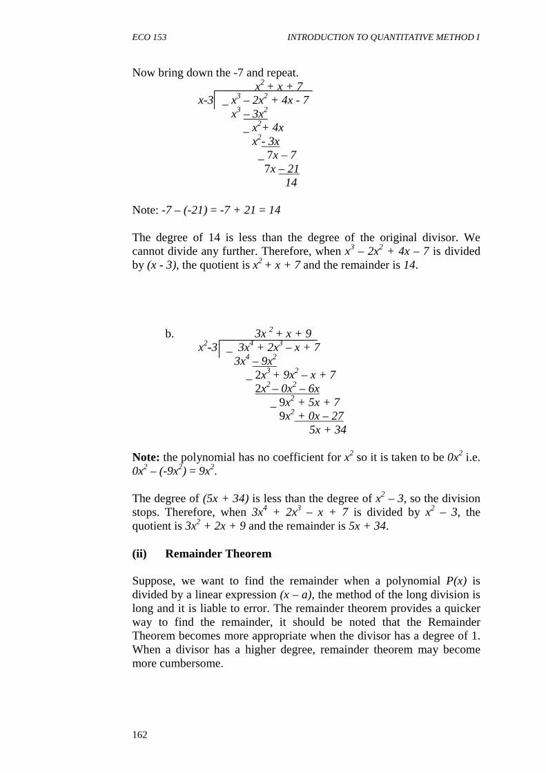
ECO 153 INTRODUCTION TO QUANTITATIVE METHOD I
162
Now bring down the -7 and repeat. x2 + x + 7 x-3 _ x3 – 2x2 + 4x - 7 x3 – 3x2 _ x2+ 4x x2- 3x _ 7x – 7
7x – 21 14
Note: -7 – (-21) = -7 + 21 = 14
The degree of 14 is less than the degree of the original divisor. We cannot divide any further. Therefore, when x3 – 2x2 + 4x – 7 is divided by (x - 3), the quotient is x2 + x + 7 and the remainder is 14.
b. 3x 2 + x + 9 x2-3 _ 3x4 + 2x3 – x + 7 3x4 – 9x2 _ 2x3 + 9x2 – x + 7 2x2 – 0x2 – 6x _ 9x2 + 5x + 7 9x2 + 0x – 27 5x + 34
Note: the polynomial has no coefficient for x2 so it is taken to be 0x2 i.e. 0x2 – (-9x2) = 9x2. The degree of (5x + 34) is less than the degree of x2 – 3, so the division stops. Therefore, when 3x4 + 2x3 – x + 7 is divided by x2 – 3, the quotient is 3x2 + 2x + 9 and the remainder is 5x + 34.
(ii) Remainder Theorem
Suppose, we want to find the remainder when a polynomial P(x) is divided by a linear expression (x – a), the method of the long division is long and it is liable to error. The remainder theorem provides a quicker way to find the remainder, it should be noted that the Remainder Theorem becomes more appropriate when the divisor has a degree of 1. When a divisor has a higher degree, remainder theorem may become more cumbersome.
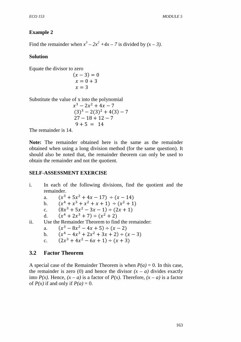
ECO 153 MODULE 5
163
Example 2 Find the remainder when x3 – 2x2 +4x – 7 is divided by (x – 3).
Solution
Equate the divisor to zero
�� − 3� = 0 � = 0 + 3 � = 3
Substitute the value of x into the polynomial
�� − 2�� + 4� − 7 (3)� − 2(3)� + 4�3�− 7 27 − 18 + 12 − 7 9 + 5 = 14
The remainder is 14.
Note: The remainder obtained here is the same as the remainder obtained when using a long division method (for the same question). It should also be noted that, the remainder theorem can only be used to obtain the remainder and not the quotient.
SELF-ASSESSMENT EXERCISE i. In each of the following divisions, find the quotient and the
remainder. a. (�� + 5�� + 4� − 17) ÷ (� − 14) b. (�� + �� + �� + � + 1) ÷ (�� + 1) c. �8�� + 5�� − 3� − 1�÷ (2� + 1) d. ��� + 2�� + 7�÷ (�� + 2)
ii. Use the Remainder Theorem to find the remainder: a. ��� − 8�� − 4� + 5�÷ (� − 2) b. ��� − 4�� + 2�� + 3� + 2�÷ (� − 3) c. �2�� + 4�� − 6� + 1�÷ (� + 3)
3.2 Factor Theorem
A special case of the Remainder Theorem is when P(a) = 0. In this case, the remainder is zero (0) and hence the divisor (x – a) divides exactly into P(x). Hence, (x – a) is a factor of P(x). Therefore, (x – a) is a factor of P(x) if and only if P(a) = 0.
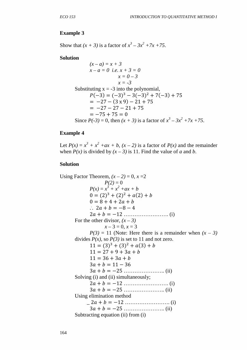
ECO 153 INTRODUCTION TO QUANTITATIVE METHOD I
164
Example 3 Show that (x + 3) is a factor of x3 – 3x2 +7x +75.
Solution
(x – a) = x + 3 x – a = 0 i.e. x + 3 = 0 x = 0 – 3 x = -3 Substituting x = -3 into the polynomial,
!�−3� = (−3)� − 3(−3)� + 7�−3�+ 75 = −27 − �3x9�− 21 + 75 = −27 − 27 − 21 + 75 = −75 + 75 = 0
Since P(-3) = 0, then (x + 3) is a factor of x3 – 3x2 +7x +75.
Example 4 Let P(x) = x3 + x2 +ax + b, (x – 2) is a factor of P(x) and the remainder when P(x) is divided by (x – 3) is 11. Find the value of a and b.
Solution Using Factor Theorem, (x – 2) = 0, x =2
P(2) = 0 P(x) = x3 + x2 +ax + b
0 = (2)� + (2)� + ��2�+ % 0 = 8 + 4 + 2� + % ... 2� + % = −8 − 4 2� + % = −12 ……………………. (i)
For the other divisor, (x – 3) x – 3 = 0, x = 3 P(3) = 11 (Note: Here there is a remainder when (x – 3) divides P(x), so P(3) is set to 11 and not zero.
11 = (3)� + (3)� + ��3�+ % 11 = 27 + 9 + 3� + % 11 = 36 + 3� + % 3� + % = 11 − 36 3� + % = −25 ………………….. (ii)
Solving (i) and (ii) simultaneously; 2� + % = −12 ……………………. (i)
3� + % = −25 ………………….. (ii) Using elimination method _ 2� + % = −12 ……………………. (i)
3� + % = −25 ………………….. (ii) Subtracting equation (ii) from (i)
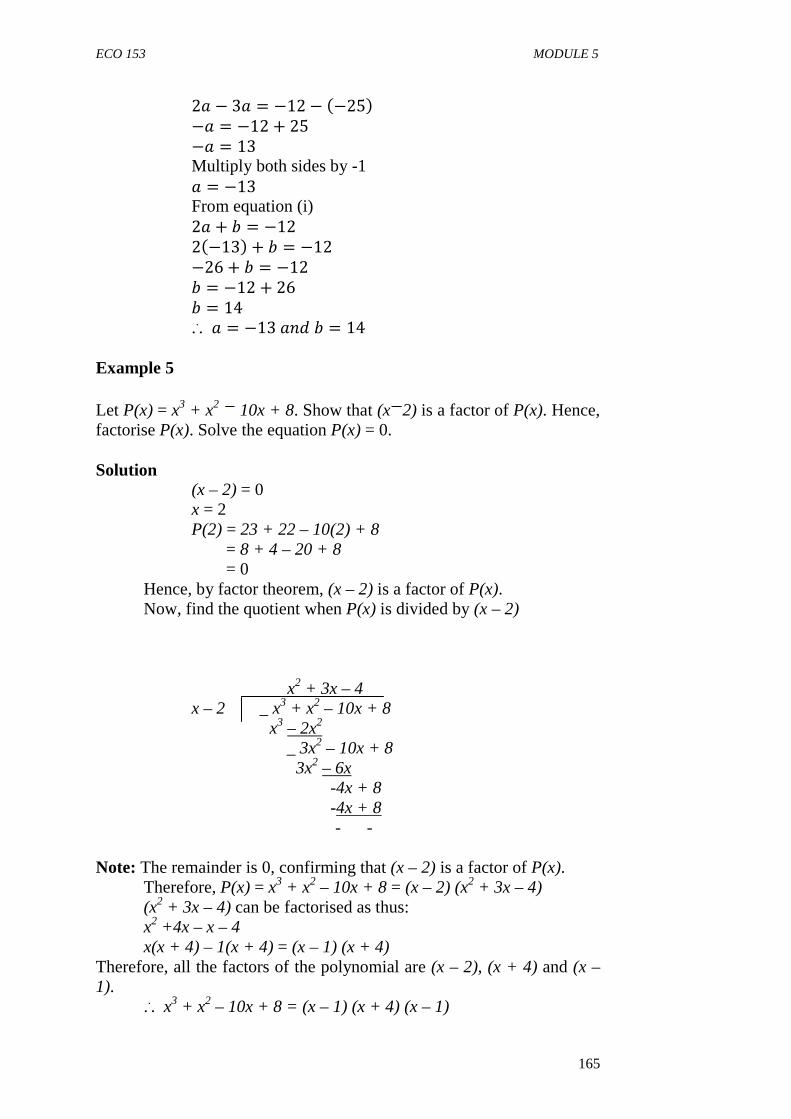
ECO 153 MODULE 5
165
2� − 3� = −12 − �−25� −� = −12 + 25 −� = 13 Multiply both sides by -1 � = −13 From equation (i) 2� + % = −12 2�−13�+ % = −12 −26 + % = −12 % = −12 + 26 % = 14 ... � = −13��% = 14
Example 5 Let P(x) = x3 + x2 10x + 8. Show that (x 2) is a factor of P(x). Hence, factorise P(x). Solve the equation P(x) = 0.
Solution
(x – 2) = 0 x = 2
P(2) = 23 + 22 – 10(2) + 8 = 8 + 4 – 20 + 8 = 0 Hence, by factor theorem, (x – 2) is a factor of P(x). Now, find the quotient when P(x) is divided by (x – 2) x2 + 3x – 4 x – 2 _ x3 + x2 – 10x + 8 x3 – 2x2 _ 3x2 – 10x + 8 3x2 – 6x
-4x + 8 -4x + 8 - -
Note: The remainder is 0, confirming that (x – 2) is a factor of P(x). Therefore, P(x) = x3 + x2 – 10x + 8 = (x – 2) (x2 + 3x – 4) (x2 + 3x – 4) can be factorised as thus: x2 +4x – x – 4 x(x + 4) – 1(x + 4) = (x – 1) (x + 4)
Therefore, all the factors of the polynomial are (x – 2), (x + 4) and (x – 1).
... x3 + x2 – 10x + 8 = (x – 1) (x + 4) (x – 1)
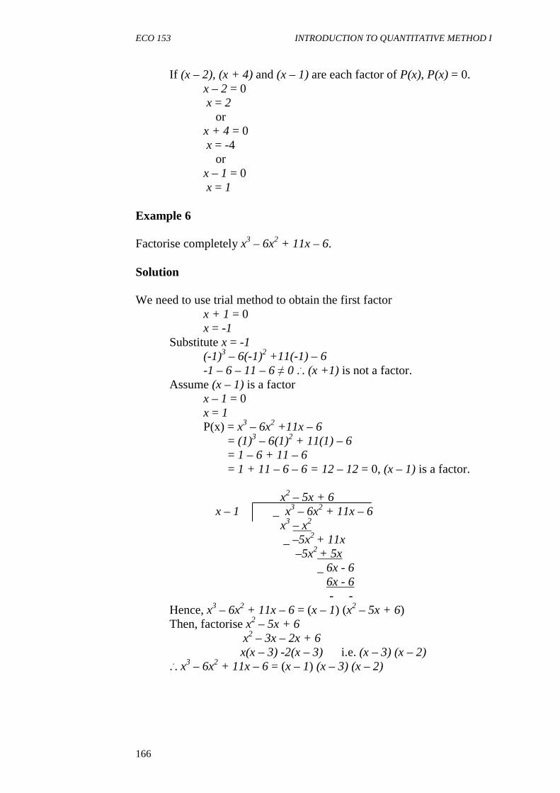
ECO 153 INTRODUCTION TO QUANTITATIVE METHOD I
166
If (x – 2), (x + 4) and (x – 1) are each factor of P(x), P(x) = 0. x – 2 = 0 x = 2 or
x + 4 = 0 x = -4 or
x – 1 = 0 x = 1
Example 6 Factorise completely x3 – 6x2 + 11x – 6.
Solution We need to use trial method to obtain the first factor
x + 1 = 0 x = -1 Substitute x = -1 (-1)3 – 6(-1)2 +11(-1) – 6 -1 – 6 – 11 – 6 ≠ 0 ... (x +1) is not a factor. Assume (x – 1) is a factor x – 1 = 0 x = 1 P(x) = x3 – 6x2 +11x – 6 = (1)3 – 6(1)2 + 11(1) – 6 = 1 – 6 + 11 – 6 = 1 + 11 – 6 – 6 = 12 – 12 = 0, (x – 1) is a factor. x2 – 5x + 6
x – 1 _ x3 – 6x2 + 11x – 6 x3 – x2 _ –5x2 + 11x –5x2 + 5x _ 6x - 6 6x - 6 - - Hence, x3 – 6x2 + 11x – 6 = (x – 1) (x2 – 5x + 6) Then, factorise x2 – 5x + 6 x2 – 3x – 2x + 6 x(x – 3) -2(x – 3) i.e. (x – 3) (x – 2) ... x3 – 6x2 + 11x – 6 = (x – 1) (x – 3) (x – 2)

ECO 153 MODULE 5
167
SELF-ASSESSMENT EXERCISE i. In these questions, show that the linear expression is a factor of
the polynomial: a. (x – 1), x3 – x2 + 3x – 3 b. (x + 2), x3 + 4x2 – x – 10
ii. Which of the following are factor of x3 + 3x2 – 5x – 10: a. x – 1 b. x – 2 c. x + 5
iii. (x + 1) is a factor of x3 – 8x2 – ax + 4. Find the value of a. iv. The remainder when x3 – 4x2 – ax + 5 is divided by (x – 3) is 8.
Find a? v. When x3 + 3x2 + ax + b is divided by (x +1), the remainder is 5,
and when it is divided by (x – 2), the remainder is 8. Find a and b?
vi. (x – 1) and (x – 2) are both factors of x3 + ax2 + bx + 4. Find a and b?
vii. In question a – c below, show that the linear expression is a factor of the polynomial. Hence, factorise the polynomial:
a. (x – 2), x3 + 3x2 – 4x – 12 b. (x – 4), x3 – 9x2 + 26x – 24 c. (x + 2), 3x3 + 5x2 – 4x – 4
viii. Use the results obtained in 7(a), (b) and (c) to solve for the following equations:
a. x3 + 3x2 – 4x – 12 = 0 b. x3 – 9x2 + 26x – 24 = 0 c. 3x3 + 5x2 – 4x – 4 = 0
4.0 CONCLUSION
Polynomials can also divide one another as much as the polynomial has a higher power relative to the quotient. In diving one polynomial by the other, it is likely there exist a remainder. Hence, given P(x) as the polynomial, D(x) as divisor and Q(x) as the quotient while R is the remainder. The relationship which exists among the four terms can be expressed as:
P(x) = D(x) . Q(x) + R, just as we have in normal division of positive whole number. For instance, 100 ÷ 7 gives 14 remainder 2; which implies that: 100 = (7 x 14) + 2
When a divisor divides a polynomial without a remainder, that divisor is a factor of the polynomial, hence P(x) = D(x) + Q(x), since R = 0. Such factor if equated to zero and a value is obtained, if the value obtained is substituted to the polynomial, we get a value of zero.
ECO 153 INTRODUCTION TO QUANTITATIVE METHOD I
168
5.0 SUMMARY
Division in polynomial can take two forms namely long division and the Remainder Theorem. The long division is used to obtain both the quotient and the remainder while remainder theorem is specifically used to the remainder. The long division is used for division of two polynomials whether the divisor is of degree 1 (linear expression) or more than degree. However, the remainder theorem is best applied when the divisor is of degree 1. The divisor is set to zero to obtain the value of the variable and thereafter substitute the value into the polynomial. The value obtained is the remainder from the division of the polynomial by the linear expression (the divisor).
When no remainder is left, the divisor is said to be a factor of the polynomial. Other factors of the polynomial can be obtained by factorising the quotient obtained.
A polynomial may be expressed in terms of one or two other unknowns apart from the main variable. To obtain these unknown, the factors (with or without remainder) is substituted into the polynomial to obtain either a linear equation or a set of simultaneous equation. This equation or equations are solved simultaneously to obtain the values of the unknown. 6.0 TUTOR-MARKED ASSIGNMENT
1. Given that���� = �(��)��� . Find the value of f(1).
(Hint: you may have to factorise and perform necessary division before you substitute).
2. Given that f(x) = 5x3 – 3x2 +4x + 7, g(x) = 6x2 + 5x – 4 and h(x) = 8x3 + 5x – 2. Find (i) f(x) + 2g(x) – 3h(x)
(ii) f(x) . g(x) – 3h(x) (iii) [g(x)]2 ÷ h(x) (iv) f(x) ÷ g(x) 3. a) Find the remainder when 2x2 – 5x + 6 is divided by (x – 3). b) Find the quotient and the remainder when f(x) = 3x3 – 2x2 +
4x + 5 is divided by (x – 1). c) Factorise completely x3 – 6x2 +11x – 6. 4. Let p(x) = x2 – 3x – 1 and q(x) = 2x – 3. Find the following,
simplifying your answers: (a) p(x) + q(x) (b) p(x) – q(x) (c) p(x) .
q(x) 5. Find the following; simplifying your answer a. (2x – 3) (x + 7)
ECO 153 MODULE 5
169
b. (x2 +2x +1) (x – 8) c. (2x – 3)3 d. (2x – 3)2 (x – 1) e. (x3 + 1) (x2 – 1)
6. In each of the following divisions, find the quotient and the remainder. a. (x3 – 3x2 + 4x + 1) ÷ (x – 2) b. (x3 + 4x – 3) ÷ (x + 2) c. (16x4 + x – 3) ÷ (2x – 3) d. (2x4 + 4x – 3) ÷ x2 + 2x) e. (3x5 + 2x3 – 8) ÷ (x2 + 1) f. (2x5 + 8x2 + 7x – 3) ÷ (2x2 + 3)
7. In these divisions, use the remainder theorem to find the remainder. a. (x3 – 2x2 + 7x – 3) ÷ (x + 1) b. (x6 – x3 + 3) ÷ (x + 1) c. (x3 + x2 – x + 1) ÷ (x + 5)
8. a) The remainder when (x3 – 6x2 + 5x + a is divided by (x + 2) is 3. Find a.
b) The remainder when x4 – ax + 3 is divided by (2x – 1) is 2. Find a.
9. (x – 2) s a factor of P(x) = x3 + ax2 +bx + 6 and the remainder when P(x) is divided by (x + 3) is 30. Find a and b. 10. In question a – c below show that the linear expression is a factor of the polynomial, hence, solve the equation that follows: (i) (x + 1), x3 + x2 – 4x – 4 (ii) (x + 1), x3 – 6x2 + 5x + 12 (iii) (x – 1), 2x3 - x2 – 2x + 1. Hence, solve for the following equations: a) x3 + x2 – 4x – 4 = 0 b) (x + 1), x3 – 6x2 + 5x + 12 = 0 c) 2x3 - x2 – 2x + 1 = 0
11. Find the values of p and q if (x – 1) and (x + 2) are factor of 2x2 + px – x + q.
12. Determine the remainder if x – 4 is a divisor of x4 + 2x3 – 6x2 + 3.
13. Find the remainder and the quotient if 4x3 + 2x2 – 6x + 9 is divided by (2x + 1).
14. Find the other factors if (x + 1) is a factor of x3 + 4x2 – x – 4. 15. If f(x) = 3x + 2 and g(x) = 2x – 1. Find (a) f(x) + g(x) (b) {[f(x)]2 – 2g(x)} if x = 3. 16. Given that f(x) = -3x3 – x2 + 3x – 100. Evaluate (a) f(-3) (b)
f(5) (c) f(0)

ECO 153 INTRODUCTION TO QUANTITATIVE METHOD I
170
7.0 REFERENCES/FURTHER READING Edward, T. D. (2006). Introduction to Mathematical Economics. (3rd
ed.). Tata–McGraw – Hill. Robert, S. & Geoff, B. (2007). Excellence in Mathematics for Senior
Secondary Schools. Ibadan: Macmillian Publishers Limited. Saleh, U. A. (2003). Quantitative Techniques in Business. Maiduguri:
Compaq Publisher Limited. Stroud, K. A. (1995). Engineering Mathematics. England: Graham Burn
Publisher.
ECO 153 MODULE 5
171
UNIT 3 PARTIAL FRACTION CONTENTS 1.0 Introduction 2.0 Objectives 3.0 Main Content 3.1 Resolving Proper Rational Expression to Partial Fraction 3.2 Resolving Improper Rational Expression to Partial
Fraction 4.0 Conclusion 5.0 Summary 6.0 Tutor-Marked Assignment 7.0 References/Further Reading
1.0 INTRODUCTION
Sometimes, a polynomial divides the other not to know the quotient or the remainder but to find a simpler alternative of expressing the rational algebraic function (function of one polynomial dividing the other). A rational algebraic fraction is a quotient fraction is a quotient of two
polynomial i.e. �(�)�(�) . This could either be proper or improper. A proper
rational expression is an algebraic function whose degree of numerator
is less than that of the denominator e.g. ������� , �
����� , ����������(���) , �. . �.
An improper rational expression is the one in which the degree of the denominator is less than the degree of the numerator e.g. ��������
���� , ������(��)������ . Both the proper and improper rational expression
can be resolved to partial fraction. 2.0 OBJECTIVES At the end of this unit, you should be able to: • resolve proper rational expression into partial fraction • resolve improper rational expression into partial fraction.
ECO 153 INTRODUCTION TO QUANTITATIVE METHOD I
172
3.0 MAIN CONTENT 3.1 Resolving Proper Rational Expression into Partial Fraction
The process involved in resolving proper rational expressions to partial fraction depends on the nature of the denominator of the expression to be resolved. The four examples below are some of the simplest forms of proper rational expressions.
Example 1
Resolve into partial fraction �
�����
Solution 5
�� + � − 6 = &� + 3 + '
� − 2
Note: (x + 3) and (x – 2) are obtained when x2 + x – 6 is factorised.
i.e. x2 + x – 6 x2 + 3x – 2x – 6 x(x + 3) – 2(x + 3) (x + 3) (x – 2)
Since (x – 2) and (x + 3) are linear terms, their numerator is expressed in coefficient (A and B).
������ = �
���+ ��� , the LCM is (x + 3) (x – 2) =
x2 + x – 6 5
�� + � − 6 = &� + 3 + '
� − 2 5 = &�� − 2�+ '(� + 3)�� + 3�(� − 2)
This is as good as multiplying through by (x + 3) (x – 2) which is the same thin as x2 + x – 6
5 = &�� − 2�+ '�� + 3� 5 = &� − 2& + '� + 3'
Separating the terms 5 = −2& + 3' (Coefficients of constants) 0 = & + ' (Coeffeicients of x) Solving simultaneously, we have & + ' = 0 ………………………… (i) x 3
−2& + 3' = 5 ………………………. (ii) x 1 _ 3A + 3B = 0
ECO 153 MODULE 5
173
-2A + 3B = 5 3A – (-2A) = 0 – 5 3A + 2A = -5 5A = -5
A = �� = −1
From equation (i) A + B = 0 -1 + B = 0 B = 0 + 1 B = 1
... The expression �
����� = ����+ �
�� Substituting A and B as -1 and 1 respectively,
Then, �
����� = ����+ ���
Or �
����� = ���− �
���
Example 2
Resolve �������
���������(���) into partial fraction.
Solution
3�� − 4� + 5�� + 1��� − 3�(2� − 1) = &
� + 1 +'
� − 3 + �2� − 1
The LCM is (x + 1) (x – 3) (2x – 1) Diving through by the LCM, we have:
3�� − 4� + 5�� + 1��� − 3�(2� − 1) = &
� + 1 +'
� − 3 + �2� − 1
3�� − 4� + 5 = &�� − 3��2� − 1�+ '�� + 1��2� − 1�+ ��� + 1�(� − 3)
�� + 1��� − 3�(2� − 1)
Expanding the numerator and ignoring the denominator, we have: -
3�� − 4� + 5 = &�2�� − 7� + 3�+ '�2�� + � − 1�+�(�� − 2� − 3)
Note: You may revisit multiplication of polynomials if you do not know how the expansion in the brackets is obtained.
3�� − 4� + 5= 2&�� − 7&� + 3& + 2'�� + '� − '+ ��� − 2�� − 3�
Separating like terms 3 = 2A + 2B + C (coefficients of��) ……………………… (i)

ECO 153 INTRODUCTION TO QUANTITATIVE METHOD I
174
-4 = 7A + B – 2C (coefficients of x) ………………………. (ii) 5 = 3A – B – 3C (the constants) …………………………… (iii) Solving equations (i), (ii) and (iii) simultaneously, we have 2A + 2B + C = 3 ……………..………… (i) 7A + B – 2C = -4 ………………………. (ii) 3A – B – 3C = 5………………………… (iii) Using elimination method, From equation (i) and (ii) 2A + 2B + C = 3 ……………..………… (i) x 1 7A + B – 2C = -4 ………………………. (ii) x 2 _ 2A + 2B + C = 3 14A + 2B – 4C = -8 2A – (-14A) + C – (-4C) = 3 – (-8) 2A + 14A + C + 4C = 3 + 8 16A + 5C = 11 …………………………. (iv) From equation (ii) and (iii), eliminate (B) 7A + B – 2C = -4 ………………………. (ii) 3A – B – 3C = 5………………………… (iii)
-7A + 3A – 2C + (-3C) = -4 + (5) -4A -2C – 3C = -4 + 5 -4A – 5C = 1 ……………………………. (v) Solving equation (iv) and (v) simultaneously to obtain A and B + 16A + 5C = 11 -4A – 5C = 1 16A + (-4A) = 11 + 1 16A – 4A = 12 12A = 12 Divide through by 12
����� =
����
A = 1 From equation (v) -4A – 5C = 1 -4(1) – 5C = 1 -4 – 5C = 1 -5C = 1 + 4 -5C = 5 Divide both sides by 5
��� =
��
ECO 153 MODULE 5
175
C = -1 From any of the equations (i), (ii) or (iii), B can be obtained. From equation (i) 2A + 2B + C = 3 2(1) + 2B + (-1) = 3 2 + 2B – 1 = 3 1 + 2B = 3 2B = 3 – 1 2B = 2
' = �� = 1
Therefore, �������
���������(���) = ���� +
���+ �
��� Substituting A, B and C, we have:
3�� − 4� + 5�� + 1��� − 3�(2� − 1) = 1
� + 1 +1
� − 3 + −12� − 1
= 1� + 1 +
1� − 3 − 1
2� − 1
Example 3
Resolve ���
���� into partial fraction
Solution
x4 – 16, has to be completely factorised, let (x – 2) be a factor (x – 2) = 0 x = 2 24 – 16 = 0 ... (x – 2) is a factor. x3 + 2x2 + 4x + 8 x – 2 _ x4 – 16 x4 – 2x3 _ 2x3 – 16 2x3 – 4x2 _ 4x2 – 16 4x2 – 8x _ 8x – 16 8x - 16 - - Therefore, x4 – 16 = (x – 2) (x + 2) (x2 + 4)
Note: (x4 – 16) cannot be factorised further 16�
�� − 16 = &� − 2 + '
� + 2 + �
�� + 4
ECO 153 INTRODUCTION TO QUANTITATIVE METHOD I
176
Note: The numerator of the third component on the RHS is Cx + D. This is because when the denominator is a quadratic expression, the numerator is expressed as a linear expression.
16��� − 16 = &
� − 2 + '� + 2 +
�� + "�� + 4
Multiplying through by the LCM = (x – 2) (x + 2) (x2 + 4), we have
16� = &�� + 2���� + 4�+ '�� − 2���� + 4�+ �� +"�� − 2��� + 2� 16� = &��� + 4� + 2�� + 8�+ '��� + 4� − 2�� − 8�+ ��
+ "��� − 4� 16� = &�� + 4&� + 8&�� + '�� + 4'� − 2'�� − 8' +��� − 4�� + "�� − 4"
Separating the terms 0 = A + B + C (coefficients of x3) ……………….. (i) 0 = 2A – 2B + D (coefficients of x2) ………………… (ii) 16 = 4A + 4B – 4C (coefficients of x) ………………… (iii) 0 = 8A – 8B – 4D (constants) …………………………. (iv) From equation (iii); dividing through by 4 4 = A + B – C ... A + B = 4 + C ……………………….. (v) From (i), 0 = A + B + C Substitute A + B = 4 + C ... 0 = 4 + C + C 0 – 4 = 2C -4 = 2C
� = �� = −2
From equation (v) A + B = 4 + C A + B = 4 + (-2) A + B = 4 – 2 A + B = 2 …………………………… (vi) Eliminating C from equation (i) and (iii) + 0 = A + B + C 4 = A + B – C 0 + 4 = 2A + 2B 4 = 2A + 2B 2 = A + B (Note, this is the same as equation (vi), so no need to number it again) Eliminating D from equations (ii) and (iv) 0 = 2A – 2B + D …………………….. x 4 0 = 8A – 8B – 4D ……………………. x 1
ECO 153 MODULE 5
177
+ 0 = 8A – 8B + 4D 0 = 8A – 8B – 4D
16A – 16B = 0 A – B = 0 ……………………….. (vii) Solving (vi) and (vii) simultaneously, we have _ A + B = 2 …………………… (vi) A – B = 0 …………………… (vii) B – (-B) = 2 – 0 B + B = 2 2B = 2
' = �� = 1
From equation (vi), A + B = 2 A + 1 = 2 A = 2 -1 A = 1 Then, D can be obtained from equation (ii) since A, B and C are already known 0 = 2A – 2B + D 0 = 2(1) – 2(1) + D 0 = 2 – 2 + D 0 = 0 + D D = 0 ... A = 1, B = 1, C = -2 and D = 0. Hence, the partial fraction is resolved as thus: -
���
���� = ���+ �
���+ ��������
Substituting A, B, C and D, we have
���
���� = ���+ �
���+ (�)�������
This can be finally expressed thus: -
16��� − 16 = 1
� − 2 + 1� + 2 −
2��� + 4
Example 4
Resolve into partial fraction ��
(���)�
Solution
��(���)� = �
���+ �(���)�
ECO 153 INTRODUCTION TO QUANTITATIVE METHOD I
178
Note: The order of the denominator, if the denominator of the partial fraction is (x + a)n, then the resolved side (RHS) becomes:
�
��� + �(���)� + �
(���)� + …+ �(���)�
For instance, if you want to resolve ��(���)� , it is simplified as
� − 8(� + 4)� = &
� + 4 + '(� + 4)� + �
(� + 4)� + "(� + 4)�
Now, we can go back to example 4;
��
(���)� = ����+ �
(���)� , multiplying through by LCM = (x
+ 3)2, we have: x – 4 = A(x + 3) + B(1) x – 4 = Ax + 3A + B Separating the term, 1 = A( coefficient of x) …………………… (i) -4 = 3A + B (constants) …………………… (ii) From equation (i) A = 1 Substituting A = 1 into equation (ii) to obtain ‘B’ -4 = 3A + B -4 = 3(1) + B -4 = 3 + B -4 – 3 = B -7 = B or B = -7 ... The partial fraction becomes
��
(���)� = ����+ �
(���)� ...
��(���)� = �
���+ (�)(���)�
Hence, ��
(���)� = ����− �
(���)�
SELF-ASSESSMENT EXERCISE
i. Resolve into partial fraction ������
���������(��) ii. Resolve
���������(���) =
����+
���� into partial fraction.
iii. Given that �������������� =
����+
���� . Find A and B.
ECO 153 MODULE 5
179
3.2 Resolving Improper Rational Expression into Partial Fraction
The process of resolving an improper rational function into partial fraction involves the use of long division first. Example
Resolve �������������(��) into partial fraction.
Solution Since the degree of numerator is greater than that of the denominator, the rational function is improper; so long division should be carried out first.
�������������(��) = ��������
�������(��) = ��������������
t t2 + t – 2 _ t3 + t2 +4t t3 + t2 – 2t 6t
... �������������� = Quotient + Resolution of
(�)�(�) into partial fraction.
... �������������� = + $����( ����� ��
������
To resolve, ��
������ = �������(��)
��
������ = ������+ �
(��) Multiplying through by (t + 2) (t – 1) 6t = A(t – 1) + B(t + 2) 6t = At – A + Bt + 2B Sorting out like terms 6 = A + B (coefficient of t) …………………….. (i) 0 = -A + 2B (coefficient of constant) …………… (ii) Solving (i) and (ii) simultaneously
Adding 1 to 2 6 + 0 = B + 2B 6 = 3B, divide both sides by 3
' = 63 = 2
From equation (i)

ECO 153 INTRODUCTION TO QUANTITATIVE METHOD I
180
6 = A + B 6 = A + 2 A = 6 – 2 A = 4.
Hence, �������������� = + �
���+ ���
Example 2
Resolve ���������
����� into partial fraction.
Solution
2x x2 – x – 2 _ 2x3 – 2x2 – 2x – 7 2x3 – 2x2 – 4x 2x – 7
Hence, ���������
����� = 2� + ��������
Resolving the rational part of RHS,
���
����� = ���+ �
��� Multiplying through by (x – 2) (x + 1)
2x – 7 = A(x + 1) + B(x – 2) 2x – 7 = Ax + A + Bx – 2B
Solving the like terms 2 = A + B (coefficient of x) -7 = A – 2B (coefficient of constants) Solving (i) and (ii) simultaneously _ 2 = A + B -7 = A – 2B 2 – (-7) = B – (-2B) 2 + 7 = B + 2B 9 = 3B
' = ��
B = 3 From equation (i), 2 = A + B 2 = A + 3 A = 3 – 2 A = 1
... ���������
����� = 2� + ���+ ����
= 2� − ���+ �
���
ECO 153 MODULE 5
181
SELF-ASSESSMENT EXERCISE
i. Resolve into partial fraction ������
�����(���)� ii. Resolve
�������������(���) into partial fraction.
4.0 CONCLUSION
The resolution of a rational fraction to partial fraction can be obtained in two folds namely proper and improper fraction. For example:
��� + %� + ��� + ��(� + %) = &
(� + �) + '(� + %) ��� + %� + �
(� + �)= &(� + �) + '
(� + �)� + �(� + �)� +⋯
+ )(� + �)
��� + %� + ���� + %� = &
� + %� For improper fraction ���������
���� = #(� ��� + $����( ����� ���� , quotient is
obtained by dividing xn+1 + xn + c by xn + x. This is an improper fraction because the power of the numerator is greater than the power of denominator.
5.0 SUMMARY
Both proper and improper rational expression can be resolved into partial fraction. The major difference in the approach lies on the procedure involved. 6.0 TUTOR-MARKED ASSIGNMENT 1. Resolve each of the following into partial fraction
a. ����
������(�����) b.
�������������
c. ������
�����������
ECO 153 INTRODUCTION TO QUANTITATIVE METHOD I
182
d. ������
e. �
���� 2. Resolve
��������(���) into partial fraction.
3. Given that ���������(��) = �
��+ ���� , find x?
4. Resolve ������
���������(���) into partial fraction.
5. Resolve into partial fraction
a. ������(��)
����
b. ����
������(�����) c.
������(����)
d. �������
���
e. ������
������(����)
7.0 REFERENCES/FURTHER READING Edward, T. D. (2006). Introduction to Mathematical Economics. (3rd
ed.). Tata–McGraw – Hill. Robert, S. & Geoff, B. (2007). Excellence in Mathematics for Senior
Secondary Schools. Ibadan: Macmillian Publishers Limited. Saleh, U. A. (2003). Quantitative Techniques in Business. Maiduguri:
Compaq Publisher Limited. Stroud, K. A. (1995). Engineering Mathematics. England: Graham
Burn Publisher.
ECO 153 MODULE 5
183
UNIT 4 BINOMIAL THEOREM CONTENTS 1.0 Introduction 2.0 Objectives 3.0 Main Content 3.1 Factorials 3.2 Binomial Expansion 4.0 Conclusion 5.0 Summary 6.0 Tutor-Marked Assignment 7.0 References/Further Reading 1.0 INTRODUCTION
In Unit 1 of this module, you were introduced to expansion of algebraic terms and polynomials. Then, (a + b)2 is expanded to (a + b) (a + b) which gives a(a + b) + b(a + b) = a2 + ab + ab + b2, which finally gives a2 + 2ab + b2. The coefficient of a2 is 1, the coefficient of ab is 2 and the coefficient b2 is 1.
Sometimes, expansion of algebraic terms or polynomials may be raised to higher indices such as (a + b)4, (x – y)8, (2a – 6d)10. In such exercises, simple expansion may be too cumbersome to apply, there is need to apply the binomial expansion. 2.0 OBJECTIVES
At the end of this unit, you should be able to: • evaluate factorials • carry out expansion of higher indices using binomial expansion • state the coefficients of the terms in a binomial expansion.
3.0 MAIN CONTENT 3.1 Factorials
Factorials are very useful concepts in economics and business related issues. The factorial of a number (n) is the product of the consecutive positive integers from n to 1. For example,
�! = ��� − 1��� − 2��� − 3�… �3��2��1� 4! = 4x3x2x1 7! = 7x6x5x4x3x2x1

ECO 153 INTRODUCTION TO QUANTITATIVE METHOD I
184
Note: 7! = 7x6x5! or 7x6x5x4! or 7x6x5x4x3!
Hence, ��!�!�! = ������������������!�������!
= 12�11�10�9�8�7 = 665, 280 It should be noted that 1! = 1 and 0! = 1
SELF-ASSESSMENT EXERCISE Simplify each of the following factorials: i. 8! ii. 3! x4! iii.
�!�!�!
iv. �!�!�!
v. ��!�!�!�!
3.2 Binomial Expansions
A binomial expression is any algebraic expression which contains two terms. Example is (a + b). Higher powers of a binomial expression can be obtained by expanding the expression (a + b)n, while n is a non-negative integer,. The general theorem of expansion of (� + %) =� + ���% + ������� �
�! + ���������� ��! +⋯+
�!���(���� �!! +⋯+ %
The above is the binomial theorem for any integer value of n. Based on the above formula, it can be shown that
(� + %)� = 1 (Recall n0 = 1) (� + %)� = � + %
(� + %)� = �� + 2�% + %� (� + %)� = �� + 3��% + 3�%� + %� Note: (� + %)� = (� + %)(� + %)� = (� + %)(�� + 2�% + %�) (� + %)� = (� + %)� + (� + %)�
= (�� + 2�% + %�)(�� + 2�% + %�) (� + %)� = (� + %)� + (� + %)�
= (�� + 2�% + %�)(�� + 3��% + 3�%� + %�) ... (� + %)� = �� + 5��% + 10��%� + 10��%� + 5�%� + %�
You will observe that the result of the expansion gives an increase power of one of the terms (i.e. b) and a decreasing power in other term (a). You equally observe that the coefficients of the terms keep changing
ECO 153 MODULE 5
185
as we increase the power of the expansion. The coefficient can be soughed out from the triangle below
(� + %)�,� = 0 1 (� + %)�,� = 1 1 1 (� + %)�,� = 2 1 2 1 (� + %)�,� = 3 1 3 3 1 (� + %)�,� = 4 1 4 6 4 1 (� + %)�,� = 5 1 5 10 10 5 1 (� + %)�,� = 6 1 6 15 20 15 5 1 (� + %)�,� = 7 1 7 21 35 35 20 6 1 (� + %)�,� = 8 1 8 28 56 70 56 28 7 1 … and so on. You observe that the triangle numbers corresponding to the coefficient of terms in each expansion. For instance(� + %)� = �� + 4��% + 6��%� + 4�%� + %�, the coefficients of the terms are: - 1 for �� 4 for ��% 6 for ��%� 4 for �%� and 1 for %�, the set of the coefficient is 1 4 6 4 1, which corresponds to the value at n = 4 from the triangle. Also, (a + b)5 gives the coefficients of 1 for a5, 5 for a4b, 10 for a3b2, 10 for a2b3, 5 for a2b4 and 1 for b5. This gives the set of coefficients as 1, 5, 10, 10, 5, 1 which correspond to the values obtained when n = 5 from the triangle.
It should be noted that the values in the triangle are obtained starting with 1 adding up the preceding coefficients and ending up with 1. It should be noted from the expansion that as one component of the term increases, the other reduces. For instance, (� + %)� = �� + 4��% +6��%� + 4�%� + %� i.e. (��%� + 4��%� + 6��%� + 4�%� + ��%�. The powers of a decrease along the expansion (from 4 to 3 to 2 to 1 to 0) while the power of b increases (from 0 to 1 to 2 to 3 to 4). The coefficients 1, 4, 6, 4 and 1 can easily be obtained from the triangle. The triangle is known as Pascal’s Triangle.
Further Examples 1. Evaluate (a) (x – y)7, stating the coefficient of the terms in the
expression. 2. Find (2a + 3c)5 and state the coefficient of a3c2.
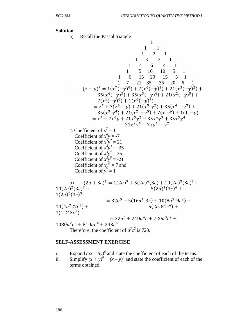
ECO 153 INTRODUCTION TO QUANTITATIVE METHOD I
186
Solution a) Recall the Pascal triangle 1 1 1
1 2 1 1 3 3 1
1 4 6 4 1 1 5 10 10 5 1
1 6 15 20 15 5 1 1 7 21 35 35 20 6 1
... (� − �)� = 1����−����+ 7����−����+ 21����−����+35����−����+ 35����−����+ 21����−����+7����−����+ 1(���−���)
= �� + 7���. −��+ 21���.���+ 35���. −���+35���. ��� + 21���. −���+ 7��.���+ 1(1.−�)
= �� − 7��� + 21���� − 35���� + 35����− 21���� + 7��� − ��
... Coefficient of x7 = 1 Coefficient of x6y = -7 Coefficient of x5y2 = 21 Coefficient of x4y3 = -35 Coefficient of x3y4 = 35 Coefficient of x2y5 = -21 Coefficient of xy6 = 7 and Coefficient of y7 = 1 b) (2� + 3�)� = 1(2�)� + 5�2����3��+ 10�2����3��� +10�2����3��� + 5�2����3��� +1�2����3��� = 32�� + 5�16��. 3��+ 10�8��. 9���+10�4��27���+ 5�2�. 81���+1(1.243��) = 32�� + 240��� + 720���� +1080���� + 810��� + 243�� Therefore, the coefficient of a3c2 is 720. SELF-ASSESSMENT EXERCISE i. Expand (3x – 5y)8 and state the coefficient of each of the terms. ii. Simplify (x + y)8 + (x – y)4 and state the coefficient of each of the
terms obtained.
ECO 153 MODULE 5
187
4.0 CONCLUSION
Factorials and binomial expansion are closely related. This is because the concept of factorial is important in binomial expansion. Binomial expansion of high powers can easily be obtained by using the Pascal theorem. 5.0 SUMMARY
Factorial of any number given is the product of the consecutive positive integer from that number to 1. High powered expansions are usually cumbersome to carry out using simple expansion procedures. Such problems are easily carried out with the use of binomial expansion theorem which is guided by the Pascal’s triangle in determining the coefficients of the terms involved. 6.0 TUTOR-MARKED ASSIGNMENT 1. Find the approximate value of a. (1.06)4 b. (0.98)4; by using the first four terms of the binomial expansion. (Hint: (1.06)4 = (1 + 0.6)4 while (0.98)4 = (1 – 0.02)4. 2. Expand (2x + 5y)6, hence state the coefficient of x4y2.
3. Simplify (a) ��!
�����! (b)
��!�!�!�!
(c) ��!�!
(d) 3! x 6! 4. Expand (a) (4x – 7y)7 (b) (2 – 4x)5
(c) (3y + 6x)4; hence state the coefficient of x3y4, x5 and x4 for the expression obtained.
7.0 REFERENCES/ FURTHER READING Edward, T. D. (2006). Introduction to Mathematical Economics (3rd ed.).
Tata–McGraw – Hill. Stroud, K. A. (1995). Engineering Mathematics. England: Graham Burn
Publishers. Zima, P. & Brown, R. L. (1979). Mathematics for Finance. Canada:
Grown Hill Ryerson Ltd.

ECO 153 INTRODUCTION TO QUANTITATIVE METHOD I
188
UNIT 5 PERMUTATION AND COMBINATION CONTENTS 1.0 Introduction 2.0 Objectives 3.0 Main Content 3.1 Arranging Objects 3.1.1 Non-Repeated Objects 3.1.2 Repeated Objects 3.2 Permutation 3.3 Combination 4.0 Conclusion 5.0 Summary 6.0 Tutor-Marked Assignment 7.0 References/Further Reading 1.0 INTRODUCTION
The concept of factorial is very useful in the process of arranging a number of different objects. For example, the four letter a, b, c and d can be arranged in different forms or ways. The first letter can be chosen in four way i.e. can take the first or second or third or fourth position. The second letter can be chosen in three ways, the third letter in two ways and the fourth letter in one way. So, the number of way is 4 x 3 x 2 x 1 = 24. You recall that, in the previous unit, 4 x 3 x 2 x 1 = 4!.
In general, the number of ways of arranging n – different objects is n (n – 1) (n – 2) … 3 x 2 x 1 = n! ways. The concept of factorial is not only useful in arranging non – repeated objects, it can also be used to know the number of ways repeated objects could be arranged as well as to provide a tool for the computation of permutations and combinations problems. 2.0 OBJECTIVES At the end of this unit, you should be able to: • determine the number of ways a non-repeated object could be
arranged • determine the number of ways a repeated object could be
arranged • apply the concept of factorials in solving Permutations and
Combination problems.

ECO 153 MODULE 5
189
3.0 MAIN CONTENT 3.1 Arranging Objects
There are two forms of arrangements of objects that the concept of factorial can assist us to obtain. These are (i) arranging non-repeated objects and arranging repeated objects. 3.1.1 Non-Repeated Objects
For a non-repeated object; the number of ways the objects can be arranged is simply n!, where n = number of distinct objects.
Example 1 In how many ways can the letters of the word “DANGER be written?”
Solution Note; The word “DANGER” has no repeated object i.e. none of the six letter is repeated. Hence, the number of ways the letters of the word can be written = 6!
= 6 x 5 x 4 x 3 x 2 x 1 = 720 ways
Example 2 In how many ways can we arrange the figures in the number: 97452018
Solution There is no repetition in the eight figures. Therefore, the number of ways it could be arranged is 8!
= 8 x 7 x 6 x 5 x 4 x 3 x 2 x 1 = 40,320 ways.
3.1.2 Repeated Objects
Suppose some of the objects are repeated. If there are r repeated objects, then these r objects can be arranged in r! ways, so we divide n! by r! to obtain the number of ways repeated objects can be arranged. This means that, given the number of objects as n and the number of repeated objects as r, the number of ways the objects can be arranged is given
as!!! .
ECO 153 INTRODUCTION TO QUANTITATIVE METHOD I
190
Example 3 In how many ways can the letters of the words “OSOGBO” be arranged?
Solution There are six letters but there are three Os. These Os can be arranged in 3! different ways.
... The number of ways “OSOGBO” can be arranged
= �!�!
= �������!�! = 120*���
Note: If there is more than one repetition, keep on dividing with the factorial of the different repetitions you can see.
Example 4 In how many ways can the word “DAMATURU” be arranged?
Solution There are 8 letters and 2 different repetitions ‘A’ and ‘U’, each of the repetition occur twice.
Therefore, number of ways of arrangement is
�!�!�! = �������������!�����!
= 10,080 ways.
Example 5 In how many ways can the word ORGANISATIONAL be arranged?
Solution
n = 14 O is written twice A is written thrice N is written twice I is written twice R, G, S, T and L are written once Therefore, numbers of the way
= ��!�!�!�!�!�!�!�!�!�!
= ��!�!�!�!�! Note 1! = 1
ECO 153 MODULE 5
191
= ����������������������������!��������������� = 1, 816, 214, 400*���
Example 6 Eda, Ngozi, Viola, Oluchi, Chinyere and Adamu are to sit on a bench. In how many ways can this be done if:
(a) Eda and Ngozi insist on sitting next to each other? (b) Eda and Ngozi refuse to sit next to each other?
Solution (a) Consider Eda and Ngozi as a single unit. There are now 5 units
instead of 6 units. The 5 units can be arranged in 5! ways since Eda and Ngozi can sit in either two ways (Eda, Ngozi) or (Ngozi, Eda). Therefore, the number of possible sitting arrangement. = 5! X 2! = (5 x 4 x 3 x 2 x 1) x 2 = 240 ways
(b) Without any restrictions, the number of ways is 6! = 720 ways.
If Eda and Ngozi refuse to sit together, then, the number of ways possible = Total number of ways without restriction minus ways possible if they insist to sit together = 720 ways – 240 ways
= 480 ways.
Example 7 In how many ways can 4 digit numbers greater than 3000 be formed using the digits 0, 1, 2, 3, 4, 5, if (a) There is no restriction? (b) If there is repetition?
Solution
(a) 3 x 5 x 4 x 3 = 180 ways Note: The first figure is 3 and not 6 because three figures can start the figure.
(b) 3 x 5 x 5 x 5 = 375 ways Note: Other figures in the products are 5 all through because any of the five numbers can take the place since repetition is allowed.
ECO 153 INTRODUCTION TO QUANTITATIVE METHOD I
192
SELF-ASSESSMENT EXERCISE i. Simplify the following by writing as single factorial expression.
a. 11! X 12 b. 13 x 12! c. 10! ÷ 10 d. 12! ÷ 132 e. 8! ÷ 56
ii. A competition lists seven desirable properties of a car and asks the entrants to put than in order of importance. In how many ways can this be done?
iii. How many five digit numbers can be made using 1, 2, 3, 4, 5, if no digit is repeated?
iv. Five men sit around a circular table. In how many ways can this be done?
v. How many arrangements are there of the letters from the following: a. AFRICA b. AMERICA c. COTTON d. MACMILLAN e. BUCKWELL f. MATHEMATICS g. REWARD
3.2 Permutation
Permutation is a way of sharing n-objects among N population in a given order. Therefore, it is mathematically written as NPn where n ≤ N. For example, suppose there are 20 children who are to receive three prizes of ₦1000, ₦500 and ₦200. In how many ways can the prize winners be chosen if no children win more than one price?
The winner of ₦1000 can be chosen in 20 ways. The winner of ₦500 can be chosen in 19 ways. The winner of ₦200 can be chosen in 18 ways.
(Note: Once someone has been chosen as the winner of ₦1000 he can no longer be chosen as the winner of ₦500 or ₦200).
Therefore, the total number of ways is 20 x 19 x 18 = 6840.
By decision, permutation is the number of ways of picking n items out of N sample space. In general, nPr is the number of picking r objects out of n sample space, in a particular order. The formula is
ECO 153 MODULE 5
193
nPr = n(n – 1) (n – 2) … (n – r + 1)
This is written as: ������…�!����!�…�����
�!�…�����
= !�!�!
Example 8 A committee has ten members. In how ways can the chairman, the secretary and the treasurer be selected?
Solution We need to choose three out of ten. As the number of posts are different, the order in which they are matters. Hence, this is a permutation. Example:
... The number of ways is 10P3
= ��!�����!
= ��!�! =
��������!�!
= 720*���
Example 9 In how many different ways can seven different books be arranged in four spaces on four spaces on a book shelf?
Solution
nPr = 7P4 = �!
����! =�!�!
= ���������!�!
= 840 ways
Example 10 How many five letter code words can be formed from the word BAKERY?
Solution
6P5 ways
= �!
��! = �!�! = 6! = 6�5�4�3�2�1 = 720*���
ECO 153 INTRODUCTION TO QUANTITATIVE METHOD I
194
SELF-ASSESSMENT EXERCISE i. In how many ways can 4 digit numbers greater than 4000 be
formed from 0, 1, 2, 3, 4, 5, 6 if: a. There is no repetition. b. There is repetition.
ii. How many telephone number of 6-digit can be formed from all the digit 0 to 9 if:
a. No telephone number must begin with zero and repetition is not allowed.
b. Repetition of digits is not allowed. c. Repetition of digits is allowed.
iii. How many other telephone numbers starting with 0 can be formed from Bola’s phone number which is 08035725368?
iv. Evaluate the following without using a calculator a. 4P3 b. 5P2 c. 9P2
v. A class has 18 pupils. In how many ways can a 1st, 2nd, 3rd and 4th prizes be awarded?
vi. There are 16 books on a library shelf. How many ways can a student borrow four of them?
vii. How many three digit numbers can be made from the digits 1, 2, 3, 4, 5, 6, 7, 8 if no digit is repeated.
viii. From a class of 19 students, six are to be selected as a member of a committee. In how many ways can this be done?
3.3 Combination
Permutation and combination are closely related concepts. While permutation deals with the number of ways of picking r objects out of n in a particular order, combination is concerned with the number of ways of choosing r objects out of n objects in any order.
Suppose that the prizes given to students are of equal values. That is no one is considered better than the other, which means it does not matter in which order the prize winners are named. Hence, the number of ways is divided by the number of ways of ordering the 3 prize winners. For instance, suppose there are 20 children to receive 3 prizes, in how many ways can the prizes be won?
This can be 120C3 = 20P3 ÷ 3 That is nCr = nPr ÷ r!
nPr = !
�!�! ... nCr =
!�!�! ÷ r = !
�!�! � �!! ... nCr =
!!!�!�!
ECO 153 MODULE 5
195
Example 11 A committee has ten members. There is to be a subcommittee of three. In how many ways can this be chosen?
Solution The three sub-committee members are equal. So, the order in which they are chosen does not matter.
Hence, this is a Combination example. ... The number of ways = 10C3
10C3 = ��!
�!�����! = ��������!�������! = 120*���
Example 12 A school committee is to be formed. There are eight eligible girls and six eligible boys. In how many ways can the committee be formed if there are four girls and three boys?
Solution
The number of ways of selecting the girls is 8C4
8C4 = �!
�!����! = ���������!���������! = 28 ways
The number of ways of selecting the boys is 6C3
6C3 = �!
�!����! =�������!�������! = 20 ways
... The committee can be chosen in (28 x 20) ways = 1400 ways
Example 13 A committee of five is to be chosen from ten men and eight women. In how many ways can this be done if there must be at least one man and at least one woman?
Solution Without any restriction, the number of ways is 18C5
If there is at least one man and at least one woman, the committee cannot be all-women or all-man. Number of all women committee = 8C5 Number of all men committee = 10C5 With the consideration of the restriction, the number of ways is = 18C5 – 8C5 – 10C5 = 8,568 – 56 – 252 = 8260 ways
ECO 153 INTRODUCTION TO QUANTITATIVE METHOD I
196
SELF-ASSESSMENT EXERCISE i. Evaluate the following without a calculator
a. 4C2 b. 5C3 c. 6C3 ii. How many ways can a committee of two men and three women
be selected from groups of eight men and seven women? iii. A library shelf contains ten novel and eight biographies. In how
many ways can a borrower choose three novels and two biographers?
iv. A football tournament is to be arranged between teams from Africa and Europe. There will be four African teams chosen from eight national sides and four European teams chosen from ten national sides. How many possible selections are there?
v. A committee of six is to be formed by a state governor from nine state commissioners and three members of the State's House of Assembly. In how many ways can the members be chosen so as to include one member of the House of Assembly?
4.0 CONCLUSION
The concept of factorial, permutation and combination are interwoven and interrelated. They are specifically used to determine the number of way an arrangement or selection can be done. 5.0 SUMMARY
The number of ways of arranging n different objects is n!. If a particular object is repeated k times, the number of ways is divided by k!. If an object is arranged in a circle rather than a row, the number of ways (n – 1)!. The number of ways of picked r objects out of n objects in a
particular order is nPr = !
�!�! while the number of ways of picking r
objects out of n objects, in any order is nCr = !
�!�!!! . If the selections
are to be made from two different sets, then we multiply together the relevance permutations and combinations. 6.0 TUTOR-MARKED ASSIGNMENT 1. Simplify (a) 11! (b)
�!�!�! (c)
��!����!
2. Simplify the following by writing as single factorial expressions. a) 10 x 9! b) 72 x 7! c) 110 x 9! d) 13! ÷ 156
ECO 153 MODULE 5
197
3. How many arrangements are there of the letters from the following: a) LAGOS b) NIGERIA c) AUSTRALIA d) HORROR e) SOLOMON f) EGYPTIAN
4. Eight people are to sit in a row. In how many ways can this be done in the following cases? a) Two particular people must sit next to each other. b) Two particular people must not sit next to each other.
5. Evaluate the following without calculator a) 6P2 b) 7C3 c) 7P5 d) 10C4 e) 8P3 6. In a competition, the entrants have to list the three most important
properties of a computer from a list of eight properties. In how many ways can this be done? a) If the three properties must be in the correct order? b) If the order of the three properties does not matter?
7. A tennis team is to contain three men and two women. In how many ways can the team be selected from a club with 15 men and 9 women?
8. A committee of five is chosen from A, B, C, D, E, F and G. In how many ways can this be chosen? a) If both A and B must be on the committee. b) If neither A or B must be on it, but both.
9. An examination consists six part A questions and seven part B questions. A candidate must attempt five questions. In how many ways can this be done? a) Without any restriction? b) If there must be two questions from part A and three question from part B.
10. A box containing 4 black, 3 white and 5 yellow balls are taken out of the box and arranged in a row from left to right. In how many ways can this arrangement be made?
7.0 REFERENCES/FURTHER READING Robert, S. & Geoff, B. (2007). Excellence in Mathematics for Senior
Secondary Schools. Ibadan: Macmillan Publishers Limited. Saleh, U. A. (2003). Quantitative Techniques in Business. Maiduguri:
Compaq Publisher Limited. Stroud, K. A. (1995). Engineering Mathematics. England: Graham Bum
Publishers.

ECO 153 INTRODUCTION TO QUANTITATIVE METHOD I
198
MODULE 6 MATRICES
Unit 1 Meaning and Types of Matrices Unit 2 Matrix Operations Unit 3 Determinant of Matrices Unit 4 Inverse of Matrices and Linear Problems UNIT 1 MEANING AND TYPES OF MATRICES CONTENTS 1.0 Introduction 2.0 Objectives 3.0 Main Content 3.1 Meaning to Matrix 3.2 Types of Matrices 4.0 Conclusion 5.0 Summary 6.0 Tutor-Marked Assignment 7.0 References/Further Reading 1.0 INTRODUCTION
Sometimes, there may be a need to present numerical or non-numerical information in a succinct, compact and simplified way. One of the means of doing this in mathematics is the used of matrices. Information such as price of garment, the score in the test, sales outlets etc. can be presented in a compact rectangular form called Matrices (singular matrix).
Linear algebra permits expression of a complicated system of equations in a compact form in an attempt to provide a shorthand method to determine whether the solutions exist or not. Matrices provide a way of solving linear equations. Therefore most economic relationship especially linear relationship can be solved using matrices.
Examples of information that can be displayed in matrices are: ���ℎ��.��������� ���������������� �3 1 0
1 2 31 3 0
231
�
The above show the number of stock of fuel the transporter has in different garage.
Another example is a company with different products, provided by matrix below.
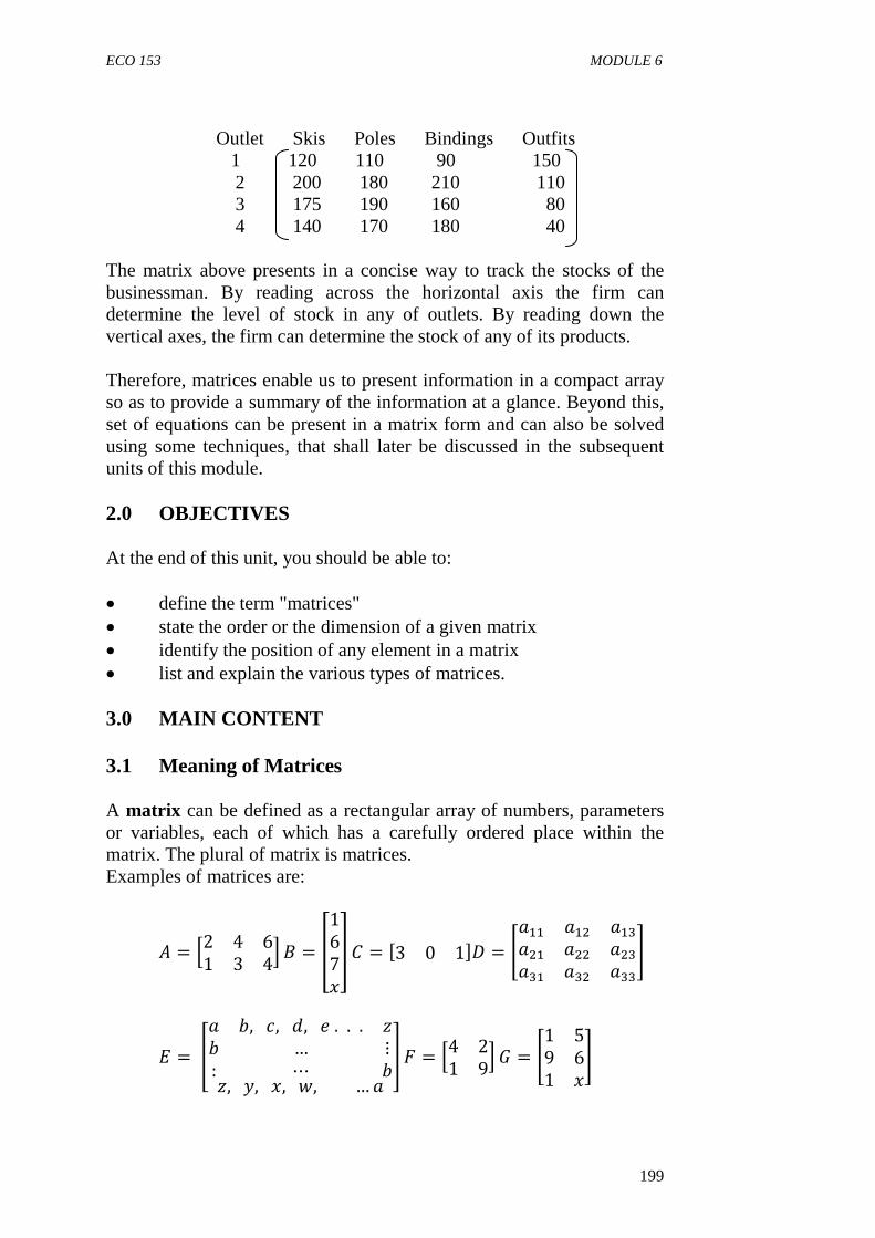
ECO 153 MODULE 6
199
Outlet Skis Poles Bindings Outfits 1 120 110 90 150 2 200 180 210 110 3 175 190 160 80 4 140 170 180 40
The matrix above presents in a concise way to track the stocks of the businessman. By reading across the horizontal axis the firm can determine the level of stock in any of outlets. By reading down the vertical axes, the firm can determine the stock of any of its products.
Therefore, matrices enable us to present information in a compact array so as to provide a summary of the information at a glance. Beyond this, set of equations can be present in a matrix form and can also be solved using some techniques, that shall later be discussed in the subsequent units of this module. 2.0 OBJECTIVES
At the end of this unit, you should be able to: • define the term "matrices" • state the order or the dimension of a given matrix • identify the position of any element in a matrix • list and explain the various types of matrices.
3.0 MAIN CONTENT 3.1 Meaning of Matrices
A matrix can be defined as a rectangular array of numbers, parameters or variables, each of which has a carefully ordered place within the matrix. The plural of matrix is matrices. Examples of matrices are:
� = �2 4 61 3 4� � = �167�� � = �3 0 1�� = ���� ��� ������ ��� ������ ��� ����
� = !� ",#, ,... $" … ⋮: ⋯ "$,%,�,&, … � ' ( = �4 2
1 9� � = �1 59 61 ��

ECO 153 INTRODUCTION TO QUANTITATIVE METHOD I
200
The number or variables in a horizontal line are called Rows, while the number variables in the vertical lines are called columns. The number of rows(r) and columns(c) defines the order or the dimensions of the matrix. That is, the order or a matrix is given by the number of rows and columns the matrix has. The dimension or order of a matrix is given by (r × c), which is read (r) by (c). The row number always precedes the column number. The order of a matrix is also called the size of the matrix.
In the examples given earlier, A is a 2 by 3 matrix i.e. (2×3) therefore it has 6 elements. B is a 4 by 1 matrix, C is a 1 by 3 matrix, D is a 3 by 3 matrix, E is a 26 by 26 matrix, F is a 2 by 2 matrix while G is a 3 by 2 matrix.
Each element in a matrix is strategically or orderly positioned to occupy a given row and a given column. This implies that no single element has less than 1 row or column; neither can any element claim more than a row or column. For example, given that:
X = 4 6 2 5 1 8 9 3 a b c d
Then, 4 is the element in row 1 and column 1, therefore its position is given as a11, 9 is the element in the 2nd row and the 3rd column, so its position is given as a34 . The position of elements in matrix X above can be presented as thus:
a11 a12 a13 a14 a21 a22 a23 a24 a31 a32 a33 a34
SELF-ASSESSMENT EXERCISE i. (a) State the number of rows and column each of the
following matrices has � = �2 4 6891 6 324� � = �� ) *+ % $, � 4
� C = 1 D = 1 2 3 4 … 20 2 2 : 3 3 : 4 : 2 20 19 18 17 … 1 � = �4 6�
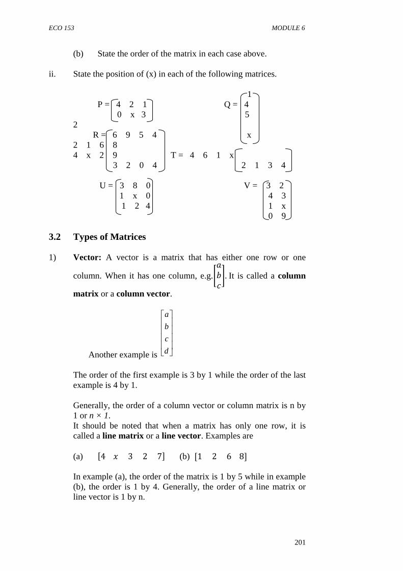
ECO 153 MODULE 6
201
(b) State the order of the matrix in each case above. ii. State the position of (x) in each of the following matrices.
1 P = 4 2 1 Q = 4
0 x 3 5 2 R = 6 9 5 4 x 2 1 6 8 4 x 2 9 T = 4 6 1 x 3 2 0 4 2 1 3 4 U = 3 8 0 V = 3 2 1 x 0 4 3 1 2 4 1 x 0 9
3.2 Types of Matrices
1) Vector: A vector is a matrix that has either one row or one
column. When it has one column, e.g.-�"#..It is called a column
matrix or a column vector.
Another example is
d
c
b
a
The order of the first example is 3 by 1 while the order of the last example is 4 by 1.
Generally, the order of a column vector or column matrix is n by 1 or n × 1. It should be noted that when a matrix has only one row, it is called a line matrix or a line vector. Examples are (a) �4�327� (b) [1268] In example (a), the order of the matrix is 1 by 5 while in example (b), the order is 1 by 4. Generally, the order of a line matrix or line vector is 1 by n.

ECO 153 INTRODUCTION TO QUANTITATIVE METHOD I
202
2) Square Matrix: A square matrix is a matrix that has the same number of rows and column. That is, a matrix is a square matrix when the number of rows it possesses equals the number of columns it has. A square matrix is any matrix whose order is m by n where m = n. Examples of a square matrix are:
A = a b B = 1 2 3 4 2 1 6 8 c d 4 5 6 C = 2 4 6 7 9 7 8 9 3 2 1 4 9 2 0 6 8 2
1 4 2 1 6 1 5 6 7 a b c d … z D = 2 2 4 1 E = b :
1 4 6 8 c c x 2 1 y : b z y x w … a In each of the examples above, the number of rows equals the number of column. For instance, in matrix A, the number of row is 2 and number of column is 2. In matrix D, the number of row is 4 and the number of column is 4. In summary, A = 2 by 2 matrix B = 3 by 3 matrix C = 4 by 4 matrix D = 26 by 26 matrix
Therefore, each of A, B, C, D and E are examples of a square matrices.
3) Null or Zero Matrixes: This is a matrix that has all its elements as zero e.g.
�0 0 00 0 00 0 0
� ,�0 00 0� ,�0 0
0 00 0
� ,[0 0] 4) Diagonal Matrix: A diagonal matrix is a square matrix that has
all its elements as zero with the exception of the elements in the leading diagonal which take other values outside zero. The elements in the leading diagonal can take other values outside zero. The elements in the leading diagonal of a square matrix are the elements in the north east direction or from left to right while
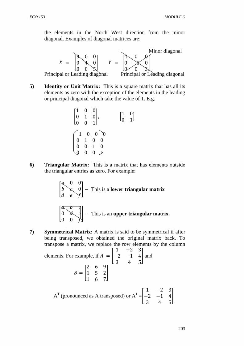
ECO 153 MODULE 6
203
the elements in the North West direction from the minor diagonal. Examples of diagonal matrices are:
Minor diagonal
/ = �3 0 00 4 00 0 5
� 0 = �4 0 00 −1 00 0 3
�
Principal or Leading diagonal Principal or Leading diagonal
5) Identity or Unit Matrix: This is a square matrix that has all its elements as zero with the exception of the elements in the leading or principal diagonal which take the value of 1. E.g.
�1 0 00 1 00 0 1
� ,�1 00 1�
1 0 0 0 0 1 0 0 0 0 1 0 0 0 0 1
6) Triangular Matrix: This is a matrix that has elements outside the triangular entries as zero. For example:
�� 0 0" # 0 1� − This is a lower triangular matrix
�� " #0 0 0 1� − This is an upper triangular matrix.
7) Symmetrical Matrix: A matrix is said to be symmetrical if after
being transposed, we obtained the original matrix back. To transpose a matrix, we replace the row elements by the column
elements. For example, if � = � 1 −2 3−2 −1 43 4 5
� and � = �2 6 91 5 21 6 7
�
AT (pronounced as A transposed) or A1 =� 1 −2 3−2 −1 43 4 5
�

ECO 153 INTRODUCTION TO QUANTITATIVE METHOD I
204
This is obtained by writing the elements on the horizontal axis e.g. 1, -2, 3 in the vertical spaces Since A = AT, A is said to be symmetrical.
Similarly BT = �2 1 16 5 69 2 8
�
You observe that B≠BT, Hence we say that B is not symmetrical.
8) Markov Matrix: This is a matrix obtained when the column or
row elements adds up to 1. It should be noted that either each of the rows or each of the columns should add up to 1 and not all the rows and the columns at the same time.
Examples of Markov Matrices are:
233341 45 2 353 45 1 35 67778 �4 3 −6
3 2 −44 −1 −2
� 4 + 3 − 6 = 13 + 2 − 4 = 14 − 1 − 2 = 1
�� + �� = 1 �� + �� = 1
9) Scalar: A Scalar is a single number used to multiply each
element of a matrix e.g.
If / = � 2 4 3−1 7 8� 2/ = � 4 8 6
−2 14 16� Hence ‘2’ is a scalar. A scalar is therefore a 1 by 1 matrix.
10) Equal Matrices: Two matrices are said to be equal if they have
the same order the same elements, elements occupy the same position and the elements have the same value.
For example:
If � = �3 40 2� � = �6 8
0 4� � = �4 0
3 2� � = �3 20 4� � = �3 4
0 2� It should be noted that B is obtained by multiplying each elements of A by 2. This does not make A to be equal to B. You should also note that A, C and D has the same order and the same elements with matrix A but the elements were not put in the same position. It should be noted that only matrices A and E are equal in all respects. Therefore we say that A = E.
ECO 153 MODULE 6
205
11) Singular Matrix: A singular matrix is a matrix whose determinant is zero. The concept of determinant shall be treated in full in the third unit of this module.
4.0 CONCLUSION
Matrix is a compact way of presenting information in a rectangular array. Every matrix has an order which tells us the number of row by the number of column it has. Members of a matrix are its element. Each element has its own position in a matrix.
5.0 SUMMARY
A Matrix is a rectangular block of numbers arranged in rows and columns. Mathematical equations (linear) can be represented in matrix form. Various types of matrices include square matrix, null matrix, diagonal matrix, identity matrix, symmetrical matrices etc. All the types of matrices have their peculiar features in terms of the nature of the element, the order of the matrix and so on.
6.0 TUTOR-MARKED ASSIGNMENT 1 Define the term “matrix”. 2 With the aid of examples, explain each of the following types of
matrices: (a) Line matrix
(b) Diagonal matrix (c) Triangular matrix (d) Symmetrical matrix (e) Square matrix
3 State ‘True’ or ‘False’ (a) All identity matrices are square matrices (b) All square matrices are identity matrices (c) The order of a column matrix is generally given as nx1. (d) The order of a matrix is the same as the position of elements
in a matrix (e) All square matrices are symmetrical
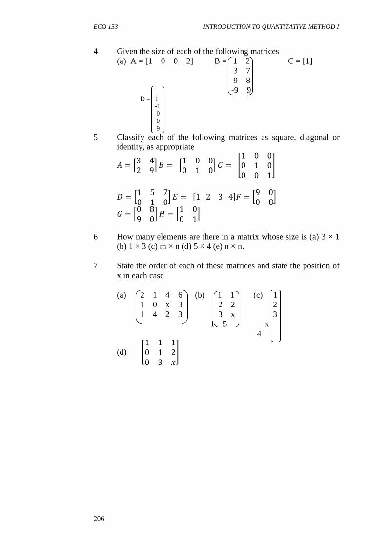
ECO 153 INTRODUCTION TO QUANTITATIVE METHOD I
206
4 Given the size of each of the following matrices (a) A = [1 0 0 2] B = 1 2 C = [1] 3 7 9 8 -9 9 D = 1 -1 0 0 9
5 Classify each of the following matrices as square, diagonal or identity, as appropriate
� = �3 42 9� � = �1 0 0
0 1 0� � = �1 0 00 1 00 0 1
�
� = �1 5 70 1 0� � = �1234�( = �9 0
0 8� � = �0 8
9 0� � = �1 00 1�
6 How many elements are there in a matrix whose size is (a) 3 × 1
(b) 1 × 3 (c) m × n (d) 5 × 4 (e) n × n. 7 State the order of each of these matrices and state the position of
x in each case (a) 2 1 4 6 (b) 1 1 (c) 1 1 0 x 3 2 2 2 1 4 2 3 3 x 3 1 5 x 4
(d) �1 1 10 1 20 3 ��
ECO 153 MODULE 6
207
7.0 REFERENCES/FURTHER READING Anthony, C. & Robert, D. (2006).Foundation Mathematics. (4thed.).
London: Pearson Hall Publisher Edward, T. D. (2004). Introduction to Mathematical Economics.
(3rded.). Delhi: Tata Mc-GrawHills Publishing Company Limited.
Hardwood, L. C. (1990).Ordinary Level Mathematics.Heinemann
Educational Books. Robert, S. & Geoff, B. (2007).Excellence in Mathematics for Senior
Secondary Schools.Ibadan: Macmillan Publishers.
ECO 153 INTRODUCTION TO QUANTITATIVE METHOD I
208
UNIT 2 MATRIX OPERATIONS CONTENTS 1.0 Introduction 2.0 Objectives 3.0 Main Content 3.1 Addition and Subtraction of Matrices 3.2 Multiplication of Matrices 3.3 Basic Identity in Matrix Operation 4.0 Conclusion 5.0 Summary 6.0 Tutor-Marked Assignment 7.0 References/Further Reading
1.0 INTRODUCTION
Elements in matrices are usually presented in quantifiable terms. Most often, we use numbers, variables or parameters to represent them. As a result of this basic mathematical operations such as addition, subtraction and multiplication are easily carried out. However in carrying out these matrix operations, certain rules principles and guidelines must be properly adhered to. This unit addresses the basic rules involved in adding, subtracting and multiplying matrices as a well as examining the basic identities in matrix operation.
2.0 OBJECTIVES
At the end of this unit, you should be able to: • carry out addition and subtraction of matrices • multiply compatible matrices • state and show the basic identities in matrix operation.
3.0 MAIN CONTENT
3.1 Addition and Subtraction of Matrices
Two or more matrices can be added together or subtracted from one another if and if only they have the same number of rows and column. This implies that addition and subtraction of matrices is only possible. If the matrices are to be added together or subtracted from one another, they must have the same order.

ECO 153 MODULE 6
209
Example 1
If � = �0 32 −1� � = �5 3
4 0� � = � 1 20 5−1 2
� Find (a) A + B (b) A – C
Solution
(a) � + � = �0 32 −1� + �5 4
2 0� = �5 74 −1�
The answer is obtained simply by adding up the corresponding terms in the rows and the columns.
(b) � − � = �0 32 −1� − � 1 2
0 5−1 2
�. This is not possible
because A andC are not in the same order. While A is a 2 by 2 matrix, C is a 3 by 2 matrix. Hence, addition or subtraction of matrices A and C is not possible.
Example 2
Given that � = �2 3 45 6 78 −9 1
� � = �3 57 82 3
� �� � = � 3 5 67 8 9−1 2 3
� Find (i) A + 2C (ii) ½A – 3C (iii) A + 4B
Solution
(i) 2� = 2 � 3 5 67 8 9−1 2 3
� = � 6 10 1214 16 18−2 4 6
�
... � + 2� = �2 3 45 6 78 −9 1
� + � 6 10 1214 16 18−2 4 6
� = � 8 13 16
19 22 256 −5 7
� (ii) ½A – 3C
�� � = �� �2 3 4
5 6 78 −9 1
� = 233341�� 2�� 3 ��
4 − �� ��67778
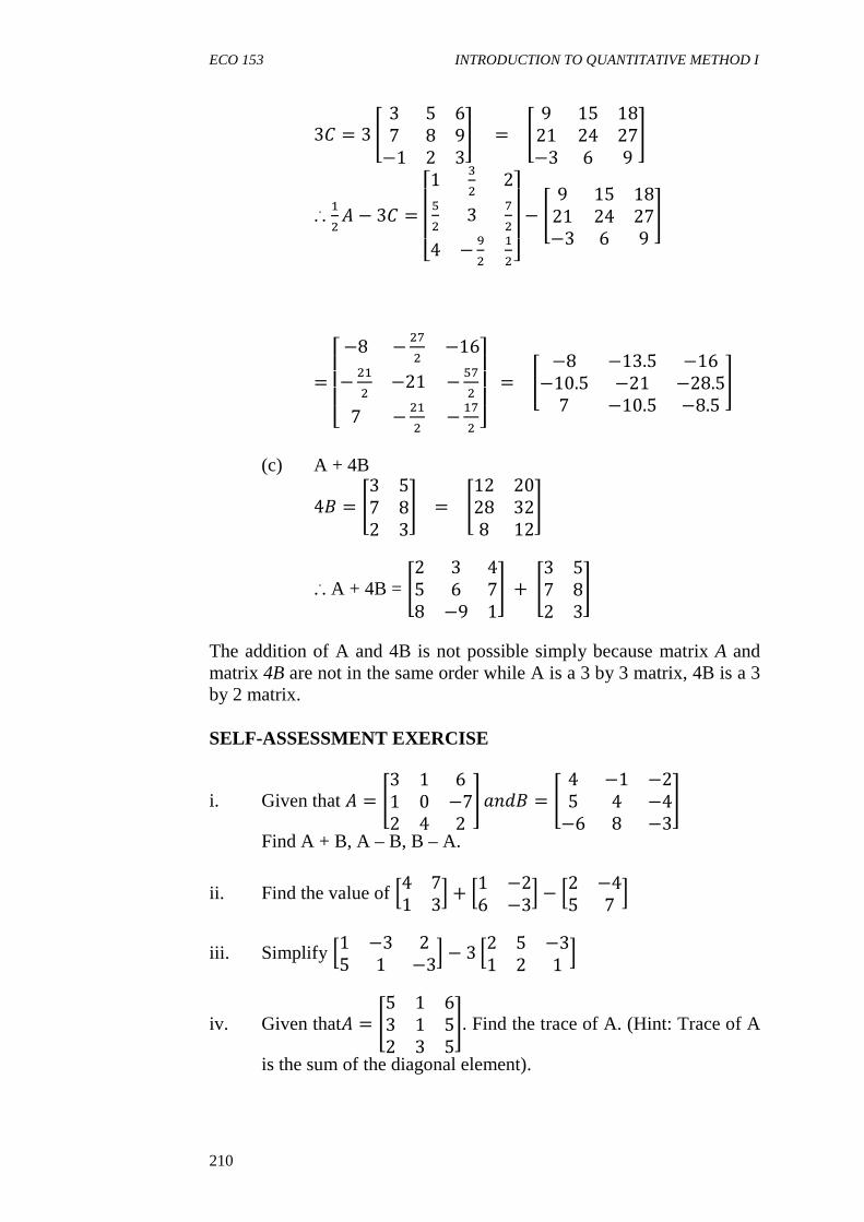
ECO 153 INTRODUCTION TO QUANTITATIVE METHOD I
210
3� = 3 � 3 5 67 8 9−1 2 3
� = � 9 15 1821 24 27−3 6 9
�
... �� � − 3� = 233341
�� 2�� 3 ��4 − �� ��67778 − � 9 15 18
21 24 27−3 6 9
�
= 23334 −8 − ��� −16− ��� −21 − ���7 − ��� − ��� 67778 = � −8 −13.5 −16
−10.5 −21 −28.57 −10.5 −8.5
� (c) A + 4B
4� = �3 57 82 3
� = �12 2028 328 12
�
... A + 4B = �2 3 45 6 78 −9 1
� + �3 57 82 3
�
The addition of A and 4B is not possible simply because matrix A and matrix 4B are not in the same order while A is a 3 by 3 matrix, 4B is a 3 by 2 matrix.
SELF-ASSESSMENT EXERCISE
i. Given that � = �3 1 61 0 −72 4 2
� �� � = � 4 −1 −25 4 −4−6 8 −3
� Find A + B, A – B, B – A.
ii. Find the value of �4 71 3� + �1 −2
6 −3� − �2 −45 7 �
iii. Simplify �1 −3 25 1 −3� − 3 �2 5 −3
1 2 1 �
iv. Given that� = �5 1 63 1 52 3 5
�. Find the trace of A. (Hint: Trace of A
is the sum of the diagonal element).

ECO 153 MODULE 6
211
v. Given that � = �3 12 −1� � = � 0 −1
−2 3 � � = � 1 4 2−1 0 1� � = � 1 1 0
−1 2 −3�. Evaluate each of the following
where possible: (a) A + 2B (b) 2C + 3D (c) 2C + 3D (d) A – B + C – D
vi. Let 9 = �1 0 32 1 02 4 −2
� �� : = �−3 2 4−2 4 02 1 −2
�
Evaluate (a) M – N (b) 2M + 3N (c) 3M – 2N
3.2 Multiplication of Matrices
Two matrices A and B are conformable for multiplication to obtain A. Bif and only if the number of columns of A is equal to the number of row of B. Similarly, A and B are conformable for multiplication to obtain B. A if and only if the number of column of B equals to the number of row of A. therefore, A. B is not equal toB. A.
Example 1
Consider the following matrices � = �2 3 45 6 7� � = � 2 4
−3 5� � = �−1 82 65 9
� and� = �1 6 8
4 2 51 3 −3
� (a) Which of these operations are possible?
(i) A.B (ii) B.A (iii) C.D (iv) B.C (v) D.A (vi) B2 (vii) C2 (viii) D2 (ix) D2 (x) A.D
(b) For each of the possible operations, obtain the results.
ECO 153 INTRODUCTION TO QUANTITATIVE METHOD I
212
Solution (a) (i) A.B is not possible because number of column of A is not
equal to number of row of B (CA = 3, RB = 2 ... CA ≠ RB). (ii) B.A is possible because number of column of B is equal to
number of row of A (CB = 2, RA = 2 ... CB = RA). (iii) C.D is not possible because number of column of C is not
equal to number of rows of D. (CC = 2, RD =3 ... CC ≠ RD). (iv) B.C is not possible because number of column of B is not
equal to number of rows of C (CB = 2, RC = 3 ... CB ≠ RD). (v) D.A is not possible because number of column of D is not
equal to number of row of A. (CD = 3, RA = 2 ... CD ≠ RA).
(vi) A.C is possible because number of column of A is equal to the number of rows of C (CA = 3, RC = 3... CA = RC).
(vii) B2 = B.B, it is possible because number of column of B equals the number of row of B (CB = RB i.e. CB = 2, RB = 2).
(viii) C2 is not possible i.e. C.C is not conformable for multiplication because number of column of C is not equal to the number of rows of C (CC = 2, RC =3 ... CC ≠ RC).
(ix) D2 = D.D is possible because the number of column of D equals to the number of rows of D (CD = RD i.e. CD = 3, RD = 3).
(x) A.D is possible because the number of column of A equals to the number of rows of D (CA = 3, RD = 3 ... CA =RD).
Note: After finding out whether multiplication is possible or not, the result of the possible multiplication is obtainable following the steps below:
Take the first element in the row of the first matrix to multiply the first element in the column of the second matrix, put an addition sign, then, use the second element in the row of the first matrix to multiply the second element in the column of the second matrix and continue in that order, until the process is completed. After that, take the first element in the row of the first matrix to multiply the first element in the second column of the second matrix, put an addition sign and then use the second element in the row of the first matrix to multiply the element in the second column of the second matrix and so on until the multiplication is exhausted. After exhausting the elements in the first row of the first matrix, the same thing is done to the elements in the second row of the first matrix. From question (a), the following operations are possible:
(i) B.A
ECO 153 MODULE 6
213
(ii) A.C (iii) B.B = B2 (iv) D.D = D2 (v) A.D
The solutions to each of them are as follow:
(i) �.� = � 2 4−3 5�.�2 3 4
5 6 7� = ; 2 × 2 + 4 × 5, 2 × 3 + 4 × 6, 2 × 4 + 4 × 7
−3 × 2 + 5 × 5, −3 × 3 + 5 × 6, −3 × 4 + 5 × 7< = �24 30 36
19 21 23�
(ii) �.� = �2 3 45 6 7�.�−1 8
2 65 9
�
= ;2 × −1 + 3 × 2 + 4 × 5, 2 × 8 + 3 × 6 + 4 × 95 × −1 + 6 × 2 + 7 × 5, 5 × 8 + 6 × 6 + 7 × 9<
= �24 7042 139�
(iii) �.� = � 2 4−3 5� .� 2 4
−3 5� = ; 2 × 2 + 4 × −3, 2 × 4 + 4 × 5
−3 × 2 + 5 × −3, −3 × 4 + 5 × 5< = � −8 28
−21 13�
(iv) �.� = �1 6 84 2 51 3 −3
�.�1 6 84 2 51 3 −3
� =� 1 × 1 + 6 × 4 + 1 × 8, 1 × 6 + 6 × 2 + 8 × 3, 1 × 8 + 6 × 5 + 8 × −34 × 1 + 2 × 4 + 5 × 1, 4 × 6 + 2 × 2 + 5 × 5, 4 × 8 + 2 × 5 + 5 × −31 × 1 + 3 × 4 + −3 × 1, 1 × 6 + 3 × 2 + −3 × 3, 1 × 8 + 3 × 5 + −3 × −3
�
= �33 42 1417 53 2710 3 32
�
(v) �.� = �2 3 45 6 7� .�1 6 8
4 2 51 3 −3
� =;2 × 1 + 3 × 4 + 4 × 1, 2 × 6 + 3 × 2 + 4 × 3, 2 × 8 + 3 × 5 + 4 × −35 × 1 + 6 × 4 + 7 × 1, 5 × 6 + 6 × 2 + 7 × 3, 5 × 8 + 6 × 5 + 7 × −3<
= �18 30 1936 63 49�
ECO 153 INTRODUCTION TO QUANTITATIVE METHOD I
214
SELF-ASSESSMENT EXERCISE
i. Let A, B and C matrices be defined as � = �4 2
1 3� � = �3 41 23 5
� �� � = �2 2 23 3 3�
Find (i) A.B (ii) B.C (iii) A.C
ii. Given that � = �10 122 6 � �� � = �7 4
4 61 3
� Find (i) A.B (ii) B.A
iii. Let / = � 2 4−6 5� 0 = �2 1 −2
1 4 0 � = = �1 34 −10 −3
�
(a) State whether each of the following operations is/are conformable.
(i) X.Y (ii) Z.Z (iii) Y.Z (iv) Z.Y (v) X2 (vi) Y2 (vii) Z.X (viii) X.Z
(b) Find the results of the conformable operations. iv. Find the results of each of the following operations. >�? �1 4 8
2 4 6� �416
� >"? �4 −4 01 −2 67 −1 2
� �−2 6 130 7 0−4 8 1
� >#?�5 6 7� �1 20 33 1
�
v. Evaluate the matrix products
(a) �3 51 4� �2 −2
7 3 � (b) � 5 2
−1 4� �3 2 25 7 −1�
(c) �0.5 0.30.1 −0.2� � 0.2 0.6
−0.3 0.4� (d) �1 3 −1� �21
0�
(e) � 3 8 51 3 0−1 2 0
� �1 2 35 −1 66 3 1
� vi. Given that � = �0 3
2 −1� ,� = �5 34 0� �� � = � 1 2
0 5−1 2
� Find (a) BA
(b) CA (c) CB
ECO 153 MODULE 6
215
3.3 Basic Identity in Matrix Operation Addition, subtraction and multiplication of matrices exhibit some properties. These properties are equally exhibited when such matrix operation are carried out with some special types of matrices. Among the commonest identity in matrix operations are:
(i) Commutative law in matrix (ii) Associative law in matrix (iii) Distributive law in matrix (iv) Identity and Null matrices relations (v) Unique properties of matrices
(i) Commutative Law in Matrix Matrix addition is commutative (that is, A + B = B + A) since matrix addition merely involves he summing of corresponding elements of two matrices of the same order. Hence, the order in which the addition takes place is inconsequential (immaterial). Similarly, A – B = -B + A
For example, if � = � 4 1117 6 � � = �3 7
6 2� � + � = � 4 + 3 11 + 7
17 + 6 6 + 2 � = � 7 1823 8 �
� + � = � 3 + 4 7 + 116 + 17 2 + 8 � = � 7 18
23 8 � ... A + B
= B + A
Likewise � − � = � 4 − 3 11 − 717 − 6 6 − 2 � = −� + � =� −3 + 4 −7 + 11
−6 + 17 −2 + 6 � = � 1 411 4�
In conclusion, � + � = � + �, � − � = −� + �
(ii) Associative Law of Matrix Since (A – B) can be converted to matrix addition A + (-B), matrix subtraction is also commutative and associative. Matrix multiplication with few exception is not commutative (that is A.B ≠ B.A). Scalar multiplication however is commutative for multiplication. If three matrices X, Y and Z are conformable for multiplication, (XY)Z = X(YZ). Subject to this condition A(B + C) = AB + AC. The associative law of matrices state that (A + B) + C = A + (B + C).
For example, if � = �6 2 79 5 3� � = �9 1 3
4 2 6� � = � 7 5 110 3 8�
>� + �? = �15 3 1013 7 9 �

ECO 153 INTRODUCTION TO QUANTITATIVE METHOD I
216
(A + B) + C = �15 3 1013 7 9 � + � 7 5 1
10 3 8� =�22 8 1123 10 17�
(B + C) = �16 6 414 5 14�
A + (B + C) = � 2 79 5 3� + �16 6 4
14 5 14� =�22 8 1123 10 17�
Therefore, (A + B) + C = A + (B + C) = �22 8 1123 10 17�
This illustrates that matrix addition is associative. It should be noted that matrix multiplication is associative, provided the proper order of multiplication is maintained (AB) C = A(BC).
(iii) Distributive Law Matrix multiplication is distributive A(B + C) = AB + AC
For example, let � = �4 7 2�� = �651
� �� � = �958
� B + C = �6 + 9
5 + 51 + 8
� = �15109
� A(B + C) = �4 7 2� �1510
9� = 4 × 15 + 7 × 10 + 2 × 9 =
148
AB = �4 7 2� �651
� = 4 × 6 + 7 × 5 + 2 × 1 = 61
AC = �4 7 2� �958
� = 4 × 9 + 7 × 5 + 2 × 8 = 87
... [AB + AC] = A[B + C] [61 + 87] = 148
Thus, for the set of matrix A, B, C, distributive law of matrix multiplication holds.
(iv) Identity and Null Matrices An identity matrix I is a square matrix which has 1 for every element on the principal or leading diagonal from left to right and zero everywhere else. Then, In denotes n by n identity matrix. The multiplication of an identity matrix with any other matrix gives the matrix back. AI = IA = A Multiplication of the identity with itself gives the identity as a result
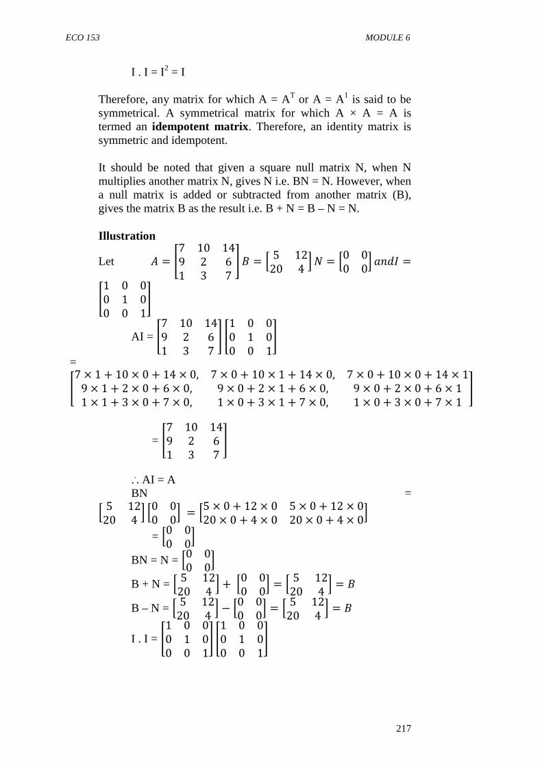
ECO 153 MODULE 6
217
I . I = I2 = I Therefore, any matrix for which A = AT or A = A1 is said to be symmetrical. A symmetrical matrix for which A × A = A is termed an idempotent matrix. Therefore, an identity matrix is symmetric and idempotent. It should be noted that given a square null matrix N, when N multiplies another matrix N, gives N i.e. BN = N. However, when a null matrix is added or subtracted from another matrix (B), gives the matrix B as the result i.e. B + N = B – N = N. Illustration
Let � = �7 10 149 2 61 3 7
� � = � 5 1220 4 � : = �0 0
0 0� �� @ =�1 0 00 1 00 0 1
� AI = �7 10 14
9 2 61 3 7
� �1 0 00 1 00 0 1
� = �7 × 1 + 10 × 0 + 14 × 0, 7 × 0 + 10 × 1 + 14 × 0, 7 × 0 + 10 × 0 + 14 × 19 × 1 + 2 × 0 + 6 × 0, 9 × 0 + 2 × 1 + 6 × 0, 9 × 0 + 2 × 0 + 6 × 11 × 1 + 3 × 0 + 7 × 0, 1 × 0 + 3 × 1 + 7 × 0, 1 × 0 + 3 × 0 + 7 × 1
�
= �7 10 149 2 61 3 7
� ... AI = A BN = � 5 1220 4 � �0 0
0 0� = �5 × 0 + 12 × 0 5 × 0 + 12 × 020 × 0 + 4 × 0 20 × 0 + 4 × 0�
= �0 00 0�
BN = N = �0 00 0�
B + N = � 5 1220 4 � + �0 0
0 0� = � 5 1220 4 � = �
B – N = � 5 1220 4 � − �0 0
0 0� = � 5 1220 4 � = �
I . I = �1 0 00 1 00 0 1
� �1 0 00 1 00 0 1
�

ECO 153 INTRODUCTION TO QUANTITATIVE METHOD I
218
�1 × 1 + 0 × 0 + 0 × 0, 1 × 0 + 0 × 0 + 0 × 0, 1 × 0 + 0 × 0 + 0 × 10 × 1 + 1 × 0 + 0 × 0, 0 × 0 + 1 × 1 + 0 × 0, 0 × 0 + 1 × 0 + 0 × 10 × 1 + 0 × 0 + 1 × 0, 0 × 0 + 0 × 1 + 1 × 0, 10 × 0 + 0 × 0 + 1 × 1
�
= �1 0 00 1 00 0 1
� = @
(v) Unique Properties of Matrices
When two singular matrices multiply themselves, the result may be a null matrix or a non-null matrix but another singular matrix. A singular matrix is the one in which a row or column is a multiple of another row or column. Example
� = � 6 −12−3 6 � � = �12 6
6 3� AB = �6 × 12 + −12 × 6, 6 × 6 + −12 × 3
−3 × 12 + 6 × 6, −3 × 6 + 6 × 3 � = �0 00 0�
A and B are both singular matrices but their product is a null matrix. Sometimes, the product of two singular matrices may not give a null matrix but another singular matrix. For example, � =�6 123 6 � � = �12 6
6 3� AB = �6 × 12 + 12 × 6 6 × 6 + 12 × 3
3 × 12 + 6 × 6 3 × 6 + 6 × 3 � = �144 7272 36�
A.B gives another singular matrix. When a singular matrix is used to multiply two other different matrices independently, the result obtained may be the same which may neither be a null matrix nor a singular matrix.
For example, if � = �4 81 2� � = �2 1
2 2� � = �−2 14 2�
A.B = �4 × 2 + 8 × 2 4 × 1 + 8 × 21 × 2 + 2 × 2 1 × 1 + 2 × 2� = �24 20
6 5 � A.C = �4 × −2 + 8 × 4 4 × 1 + 8 × 2
1 × −2 + 2 × 4 1 × 1 + 2 × 2� = �24 206 5 �
Even though B ≠ C, AB = AC. Unlike algebra, where multiplication of one number by two different numbers cannot give the same product in matrix algebra, multiplication of one matrix by two different matrices may and may not, produce the same result. In this case, A is a singular matrix.

ECO 153 MODULE 6
219
SELF-ASSESSMENT EXERCISE
i. Given that� = �4 111 3 � �� � = � 3 −11
−1 4 �. Verify that AB = I
where I is a 2 X 2 identity matrix.
ii. Calculate�3 00 2� �� "# �. Comment upon the effect of multiplying
a matrix by�3 00 2�.
iii. Given the matrices: � = �6 2 79 5 4� � = �9 1 3
4 2 �� �� � =� 7 5 :10 3 9�
Show that (A + B) + C = A + (B + C) 4.0 CONCLUSION
Matrix operation in terms of addition, subtraction and multiplication is strictly based on some rules. Once these rules are adhered to, matrices can be added together, subtracted from one another and also multiply one another. Some basic identity may evolve in the course of performing matrix operations. These identities are proven results of certain matrix operation which may be general or peculiar to some circumstances. 5.0 SUMMARY
Two matrices can be added together or subtracted from one another if they have the same order. Multiplication of two matrices A and b to produce A.B is only possible if the number of columns of A equals the number of rows of B. However, A.B ≠ B.A. Like in the set theory, commutative law, associative law and distributive laws apply to all matrices provided the matrices are conformable and/or addition
A + B = B + A = Commutative law A + (B + C) = (A + B) + C = Associative law (AB)C = A(BC) = Associative law A(B + C) = AB + AC = Distributive law
The product of an identity matrix with another matrix gives the other matrix while the product of an identity matrix with itself gives the identity matrix as the result.
When a null matrix is added or subtracted from another matrix of the same order, the result obtained is the matrix which the null matrix is added to or subtracted.
ECO 153 INTRODUCTION TO QUANTITATIVE METHOD I
220
The product of two singular matrix may give a null matrix or a non-null matrix but another singular matrix. When a singular matrix multiplies two or other different matrices independently, the result obtained may be the same. 6.0 TUTOR-MARKED ASSIGNMENT
1. Given that � = �1 22 3� ,� = �1 0 0
3 1 0� ,� = �1 2 02 3 0�
D = 1 2 0 0 E = 0 1 2 F = 0 0 1 2 2 3 0 0 0 2 3 0 0 2 3 Which of these matrices is it possible to add together?
a. Using the matrices given above, find where possible, each of the following
(i) B + E (ii) E – C (iii) D + F (iv) 4A (v) BD –E (vi) F – 2D (vii) ½ A (viii) B – ½ C (ix) B + C + E
2. Find x, y, z, w if:
�2 43 $� + �� %
3 4� = �4 4& 0� 3. Given that � = �1 0
2 1� � = �1 23 4� �� � = �4 −1
0 2 � Find A.B, B.C, A.C, A2, B2, C2, A3.
4. Given that � = �1 2 3�� = �2 3�� = � 10−1
� � = �34� and
� = �1 04 2�. Find A.C, B.D, E.D, B.E?
5. If� = �1 34 2� �� � = � 5 1
−1 0�. Find A1, B1, A.B, A1.B1, B.A?
6. (a) �� "� �� + �% ,� "� (b) � 5 � − 3�� 4 � + � 0 32 − �� −1�
7. Let � = �1 32 4� � = �1 4
2 03 1
� �� � = �2 2 01 0 3�
(i) Which of the following can be evaluated: AB, BA, AC, CA, BC and CB? (ii) Evaluate those which are possible
8. Let � = �3 20 −3�
(a) Find A2 +A (b) Find B if B + A2 = 3A
9. Let 9 = �0 21 4� �� : = �3 1
4 0� Evaluate the following
(a) M2 + N2 (b) MN +NM (c) 2MN + 3NM
ECO 153 MODULE 6
221
10. Let � = �519
� �� � = � 82−6
� Find A + B, A – B, 7A, -½B, 3A + 2B
11. Find (a) �3 25 3� ��%�
(b) �1 00 1� ��"�
(c) �14 920 1� � 19
87−73
� 12. If9 = �7 8
2 −1� �� : = � 3 2−1 4�. Find NM and MN. Comment
on your answer.
13. If � = � 1 −7−1 2 � � = � 3 7 2
−1 0 10� � = �1 0 −1 1�� =!7981
' and
� = ���001
�. Find if possible: 3A, A + B, A + C, 5D, BC, CD, AC,
CA, 5A – 2C, D – E, BA, AB, A2.
14. If @ = �1 00 1� � = � 3 7
−1 −2� � = ��%� � = �3 9 54 2 8�
Find where possible IA, AI, BI, IB, CI, IC. Comment on your answers.
15. If� = �� "# � � = ; 1� ℎ<. Find A + B, A – B, AB, BA?
16. Find (a) �−7 52 −1� ��%�
(b) �9 53 8� ��"�
17. Given � = �23 −140 1 � � = �1 2
3 −2� Find BA, B2, B2A.
18. a) Given that � = � 1 3−1 4� � = �0 −1
3 2 � b) Given � = �1 0 0
0 1 00 0 1
� � = �0 00 0� � = �12 6
6 3� State and proof any two identity familiar with A, B and C (you may introduce other matrices to conduct your proof).
19. Given that � = �7 2 65 4 83 1 9
� � = �6 25 0� � = �114
13� � = �144 � � = �8 1 10�( = [13 2]
ECO 153 INTRODUCTION TO QUANTITATIVE METHOD I
222
Determine for each of the following whether the products are defined i.e. conformable for multiplication. If so, indicate the dimensions of the product matrix. (a) AC (b) BD (c) EC (d) DF (e) CA (f) DE (g)
BD (h) CF (i) EF (j) B2 20. Crazy Teddies ells 700 CDs, 400 cassettes and 200 CD players each week. The selling price of CD is $4, cassette $6 and CD players $150. The cost to the shop is $3.25 for a CD, $4.75 for a cassette and $125 for a CD player. Find the weekly profit.
Hint: A = �700400200
� B = � 46
150� � = � 3.254.75
125.0�
TR = PT.Q TC = CT.Q π = TR – TC 7.0 REFERENCES/FURTHER READING Anthony, C. & Roberts, D. (2006).Foundation Mathematics. (4th ed.).
London: Pearson Hall Publishers. Edwards, T. D. (2004). Introduction to Mathematical Economics. (3rd
ed.). Delhi: Tata Mc-Graw Hills Publishing Limited. Robert, S. & Geoff, B. (2008).Excellence in Mathematics for Senior
Secondary School. Ibadan: Macmillan Publishers Limited.

ECO 153 MODULE 6
223
UNIT 3 DETERMINANT OF MATRICES CONTENTS 1.0 Introduction 2.0 Objectives 3.0 Main Content 3.1 Determinant of 2 by 2 Matrices 3.2 Determinant of 3 by 3 Matrices 3.3 Properties of Determinants 4.0 Conclusion 5.0 Summary 6.0 Tutor-Marked Assignment 7.0 References/Further Reading
1.0 INTRODUCTION
Determinants are usually obtained for square matrices. It is the numerical value of the matrix. The determinant of |�| of a 2 by 2 matrix called a second order determinant is derived by taking the product of the two elements on the principal diagonal and subtracting from it the product of the two element of the principal (minor diagonal).
Given � = ���� ������ ���� |�| = ����.���� − [���.���]
The determinant is a single number or scalar and it is found for square matrices. If the determinant of a matrix is equal to zero, the determinant is said to vanish and the determinant is termed singular.
The determinant of a 3 by 3 matrix
e.g. � = ���� ��� ������ ��� ������ ��� ���� is called a third order determinant and
it is obtained using a more elaborate procedure compared to a 2 by 2 matrix. Details on how the determinants of 3 by 3 matrices are obtained shall be discussed later in this unit.
The determinant of a square matrix which size is greater than 2 by 2 is called a higher ordered determinant. Examples of such matrices include 3 by 3 matrices, 4 by 4 matrices, 5 by 5 matrices etc.
ECO 153 INTRODUCTION TO QUANTITATIVE METHOD I
224
2.0 OBJECTIVES
At the end of this unit, you should be able to: • obtain the determinant of 2 by 2 matrices • obtain the determinant of 3 by 3 matrices • obtain given value(s) in a matrix, provided determinant and other
required values are given • state the properties of determinants and prove them. 3.0 MAIN CONTENT 3.1 Determinant of 2 by 2 Matrices
To evaluate the determinant of a 2 by 2 matrix given as � = �� "# �, the
following procedures are followed: (i) Multiply the elements in the leading or principal diagonal (i.e. a ×
d = ad). (ii) Multiply the elements in the minor diagonals (i.e. c × d = cd). (iii) Subtract (cd) from (ad) i.e. (ad) – (cd) gives the determinant of A,
written as|�|.
Examples
1. Find the following (a) D 2 −1−4 2 D (b) D1 3
5 −2D 2. Find the value of x for which D� 2
3 8D = 0, which type of matrix is�� 23 8�? How do you
know?
Solution
1(a) D 2 −1−4 2 D = >2 × 2? − >−4 × −1?
= 4 − >4? = 0
(b) D1 35 −2D = >−2 × 1? − >3 × 5?
= −2 − 15 = −17
2. D� 23 8D = 0
Therefore, 8x – (3 × 2) = 0 8x – 6 = 0 8x = 6
x = � = ��
The matrix is a singular matrix because its determinant is zero.
ECO 153 MODULE 6
225
SELF-ASSESSMENT EXERCISE i. Find the determinant of each of the following matrices � = �7 2
4 9� � = �4 −29 −1� � = �1 0
0 1� � = �4 22 1� �
= �8 79 2�
ii. In each of the following, find the value of x.
a) D� 12 7D = 4
b) D3� 22� 3D = D5� 2
4 −2D c) D5� 2
3� 1D = 11
3.2 Determinants of 3 by 3 Matrices
There are a number of approaches adopted in obtaining the determinant of a 3 by 3 matrix. Prominent among the approaches are:
(i) Diagonal method (ii) Expansion method
(i) Diagonal Method: When a determinant is of the size 3 by 3, the
elements of the first two columns are reproduced as if we put a mirror on the third column. This results into additional two columns to the already existing matrix. Hence, the determinant of the matrix is given as the difference between the addition of the products of the elements in the principal diagonals and the addition of the products of the elements in the non-principal diagonal for example, finds the determinant of � = �4 6 3
3 5 62 8 4
�, using the diagonal method
|�| = �4 6 33 5 62 8 4
4 63 52 8
� |�| = >4 × 5 × 6 + 6 × 6 × 2 + 3 × 3 × 8?− >2 × 5 × 3 + 8 × 6 × 4 + 4 × 3 × 6?
= >80 + 72 + 72? − >30 + 192 + 72? = 224 − 294 = −70
(ii) Expansion Method: The expansion method is used in the evaluation of 3 by 3 matrices and other higher determinants. Using this method, the following steps are followed:
Given that � = ���� ��� ������ ��� ������ ��� ����

ECO 153 INTRODUCTION TO QUANTITATIVE METHOD I
226
Step I: Take the first element of the first row, ��� and mentally delete the row and the column in which it appears. Then, multiply ��� by the determinant of the remaining elements.
���� ��� ������ ��� ������ ��� ���� �. ��� D��� ������ ���D =�������.��� − ���. ���� Step II: Take the second element of the first row ��� and mentally delete the row and column in which it appears. Then, multiply ��� by −1 times determinant of the remaining elements.
���� ��� ������ ��� ������ ��� ���� �. ��� D��� ������ ���D =�������.��� − ���. ���� Step III: Take the third element of the first row, ��� and mentally delete the row and the column in which it appears. Then, multiply ��� by the determinant of the remaining elements.
���� ��� ������ ��� ������ ��� ���� �. ��� D��� ������ ���D =�������.��� − ���. ���� Step IV: Obtain the sum of the results derived from step I, II, and III above.
Hence, |�| = �������.��� − ���.���� − �������. ��� −���.���� + �������. ��� − ���.���� Note: The sign alternates as follows !+ − +
− + −+−
−+
+−
−+−+
' and so on.
Example 1
Given that � = E4 6 33 5 62 8 4
E = 4 D5 68 4D − 3 D6 3
8 4D + 2 D6 35 6D
= 4>20 − 48? − 3>24 − 24? + 2>36 − 15? = 4>−28? − 3>0? + 2>21? = −112 − 0 + 42 = −70 A is a non-singular matrix because|�| ≠ 0.
Note: The same solution is obtained using the two methods for the same question.
ECO 153 MODULE 6
227
Example 2 Solve for x given that
-� � �0 � + 2 20 2 � − 1
.is singular matrix.
Solution
If -� � �0 � + 2 20 2 � − 1
. is singular matrix, then F� � �0 � + 2 20 2 � − 1
F = 0
... � D� + 2 22 � − 1D − � D0 2
0 � − 1D + � D0 � + 20 2 D = 0 ��>� + 2?>� − 1? − 4� − ��0>� − 1? − >2 × 0?�
+ ��0.2 − >0. � + 2?� = ���� + � − 2 − 4� − ��0 − 0� + ��0 − 0� = 0 ���� + � − 6� = 0
Factoring �>�� + 3� − 2� − 6? = 0 �G�>� + 3? − 2>� + 3?H = 0 �>� + 3?>� − 2? = 0 Hence, x = 0, or x + 3 = 0 x = 0 – 3 = -3; or x – 2 = 0 x = 0 + 2 x = +2
Therefore, forF� � �0 � + 2 20 2 � − 1
F = 0, x can either be 0, -3 or +2.
SELF-ASSESSMENT EXERCISE i. Find the determinants of these matrices
(a) �2 1 01 −3 41 0 3
� >"? �0 3 25 6 00 3 7
� ii. Find E2 1 3
4 0 05 6 7
E + E−3 0 15 1 01 −2 1
E iii. Solve for x in the matrix below E 0 � 0� − 1 1 0
5 6 � + 1E = 0

ECO 153 INTRODUCTION TO QUANTITATIVE METHOD I
228
iv. Use expansion method to obtain the determinant of B, given that
B = !4 −2 61 0 202
26
4−1
341−3
'
3.3 Properties of Determinants
The following properties of determinants provide the ways in which a matrix can be manipulated to simplify its elements or reduced part of them to zero, before evaluating the determinant.
(i) Adding or subtracting any non-zero multiple of one row (or
column) from another row (or column) will have no effect on the determinant.
e.g.� = ;�� "��� "�< |�| = ��"� − ��"�
Also, I� + ��� "� + �"��� "� I = ��"� − ��"� = |�|
(ii) Interchanging any two rows of columns or a matrix will change the sign, but not the absolute value of the determinant.
e.g.� = �2 46 8� ,� = �4 2
8 6� |�| = >8 × 2? − >6 × 4? = 72 − 24 = 48 |�| = >4 × 6? − >8 × 9? = 24 − 72 = −48
(iii) Multiplying the elements of any row or column by a constant will cause the determinant to be multiplied by the same constant.
e.g./ = �2 14 3� 0 = �2 × 5 1
4 × 5 3� = �10 120 3� |/| = >2 × 3? − >4 × 1? = 6 − 4 = 2 |0| = >10 × 3? − >20 × 1? = 30 − 20 = 10
Note: As a result of multiplication of the elements of the first column of X by 5 to obtain Y, the determinant of Y is 5 times the determinant of X.
(iv) The determinant of a triangular matrix i.e. a matrix with zero
elements everywhere above or below the principal diagonal equals to the products of the elements in the principal diagonal.
e.g. If � = �1 0 02 4 03 8 2
� R is a lower triangular matrix, |�| = 1 × 4 × 2 = 8 or

ECO 153 MODULE 6
229
|�| = E1 0 02 4 03 8 2
E = 1 D4 08 2D − 0 D2 0
3 2D + 0 D2 43 8D
= 1>8 − 0? − 0>4 − 0? + 0>16 − 12? = 1>8? − 0>4? + 0>4? = 8 − 0 + 0 = 8
(v) The determinant of a matrix equals to the determinant of its transpose
e.g.� = �1 0 02 4 03 8 2
� � = �1 2 30 4 80 0 2
� ... |�| = E1 2 3
0 4 80 0 2
E = 1 D4 80 2D − 2 D0 8
0 2D + 3 D0 40 0D
= 1>8 − 0? − 2>0 − 0? + 3>0 − 0? = 1>8? − 2>0? − 3>0?
= 8 − 0 + 0 = 8 ∴ |�| = |�|
(vi) If all the elements of any row or column are zero, the determinant
is zero.
e.g.J = �3 04 0�... |J| = >3 × 0? − >4 × 0? 9 = �0 0 0
2 1 36 −8 4
� ... |9| = 0 D 1 3−8 4D − 0 D2 3
6 4D +0 D2 1
6 −8D = 0�4 − >−24?� − 0>8 − 18?
+ 0>−16 − 6?= 0>4 + 24?− 0>−10?+ 0>−22?
= 0 + 0 − 0 = 0
(vii) If two rows or columns are identical or proportional, i.e. linearly dependent, the determinant is zero.
e.g. if � = �2 34 6� , |�| = >2 × 6 − 4 × 3? = 12 − 12 =
0 if� = �7 8
7 8� , |�| = >7 × 8? − >7 × 8? = 0
ECO 153 INTRODUCTION TO QUANTITATIVE METHOD I
230
4.0 CONCLUSION
This unit has exposed you to the techniques involved in obtaining determinant of square matrices. A good attempt has been made to expose you to the number of properties of determinants with adequate illustrations and examples. 5.0 SUMMARY
Determinants are applicable to square matrices only. If� = �� "# �, the
determinant of A written as|�| = >�. ? − (#. ). There are alternative approaches of obtaining the determinant of a 3 by 3 matrices. Common among them are the diagonal method and the expansion method. The diagonal method involves addition to the original matrix, the elements in the first two column of a 3 by 3 matrix. Then, the sum of the products of elements in the non-leading diagonal is subtracted from that in the
leading diagonal. For the expansion method, E� " # 1� ℎ � E = � D 1ℎ � D −" I 1� � I + # I � ℎI
A number of properties of determinants provide the ways in which square matrices can be manipulated to simplify its element to give a specific result. 6.0 TUTOR-MARKED ASSIGNMENT
1. Given that � = �2 1 34 0 05 6 7
� �� � = �−3 0 15 1 01 −2 1
� Find |3� − 2�| 2. Given that E 0 0 � + 1
1 � − 2 6� − 3 6 7E = 0
3. Solve for x in the following
(a) D 1 �−2 4D = 0>"? D� 1
0 2D = D3 12 �D
4. Given thatD2 3� ��D = 12. Find the possible values of x.
5. Given that �∝ +1 −103 ∝ −10� is a singular matrix. Find the value
of∝.
6. Given thatB = �1 34 5� A = �2 4
3 0�. Find|B� + 2A − 2BA�|.
ECO 153 MODULE 6
231
7. Outline any four properties of determinants with appropriate illustrations.
8. Given thatD� − 4 56 � + 3D = 5� + 15. Find the value(s) of x
7.0 REFERENCES/FURTHER READING Anthony, C. & Robert, D. (2006).Foundation Mathematics. (4th ed.).
London: Pearson Hall Publisher. Edward, T. D. (2004). Introduction to Mathematical Economics. (3rd
ed.). Delhi: Tata, Mc-Graw Hills Publishers. Elayn, M. (2003). Introductory Algebra. (2nd ed.). New Jersey:
Prentice-Hall Inc. Usman, A. S. (2005). Business Mathematics. Lagos: Apex Books
Limited.

ECO 153 INTRODUCTION TO QUANTITATIVE METHOD I
232
UNIT 4 INVERSE OF MATRICES AND LINEAR PROBLEMS CONTENTS 1.0 Introduction 2.0 Objectives 3.0 Main Content 3.1 Inverse of 2 by 2 Matrices 3.2 Inverse of 3 by 3 Matrices 3.3 The Use of Matrix Inversion in Solving Simultaneous Linear Equations 4.0 Conclusion 5.0 Summary 6.0 Tutor-Marked Assignment 7.0 References/Further Reading
1.0 INTRODUCTION
In the earlier units, we have added, subtracted and multiplied matrices. To divide matrices, we need some definitions. The identity matrix I is such that IA = AI = A for all matrices A which have the same size or order as I.
For 2 by 2 matrices, I = �1 00 1� and
For 3 by 3 matrices, I = �1 0 00 1 00 0 1
�
To divide by a number is equivalent to multiplying it by its reciprocal. For example, to divide by 2 is the same as multiply by ½. Hence, we define the inverse of a matrix A, so that dividing by A is the same as multiplying by its inverse. Recall that the inverse of 2 is ½ and the inverse of ½ is 2. Similarly, if we invert a matrix twice, we get the original matrix. So, the inverse of A-1 is A itself. Here, the superscript ‘-1’ should not be read as power but as a notation for the inverse of matrix.
It should be noted that an inverse A-1, which can be found only for a square, non-singular matrix is a unique matrix satisfying the relationship.
AA -1 = I = A-1A
Multiplying a matrix by its inverse reduces it to an identity matrix. Thus, the inverse matrix in linear algebra performs much the same function as the reciprocal in ordinary algebra. The formula for deriving the inverse
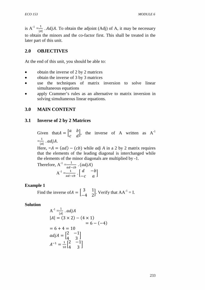
ECO 153 MODULE 6
233
is A-1 =�|�| .� K�. To obtain the adjoint (Adj) of A, it may be necessary
to obtain the minors and the co-factor first. This shall be treated in the later part of this unit. 2.0 OBJECTIVES
At the end of this unit, you should be able to: • obtain the inverse of 2 by 2 matrices • obtain the inverse of 3 by 3 matrices • use the techniques of matrix inversion to solve linear
simultaneous equations • apply Crammer’s rules as an alternative to matrix inversion in
solving simultaneous linear equations. 3.0 MAIN CONTENT 3.1 Inverse of 2 by 2 Matrices
Given that� = �� "# �, the inverse of A written as A-1
=�|�| .� K�.
Here, =� = >� ? − (#") while adj A in a 2 by 2 matrix requires that the elements of the leading diagonal is interchanged while the elements of the minor diagonals are multiplied by -1.
Therefore, A-1 =� ���� . (� K�)
A-1 =� ���� . � −"
−# � �
Example 1
Find the inverse of� = � 3 1−4 2�. Verify that AA-1 = I.
Solution
A-1 =�|�| .� K�
|�| = >3 × 2? − >4 × 1? = 6 − >−4?
= 6 + 4 = 10
� K� = �2 −14 3 �
��� = ��� �2 −14 3 �
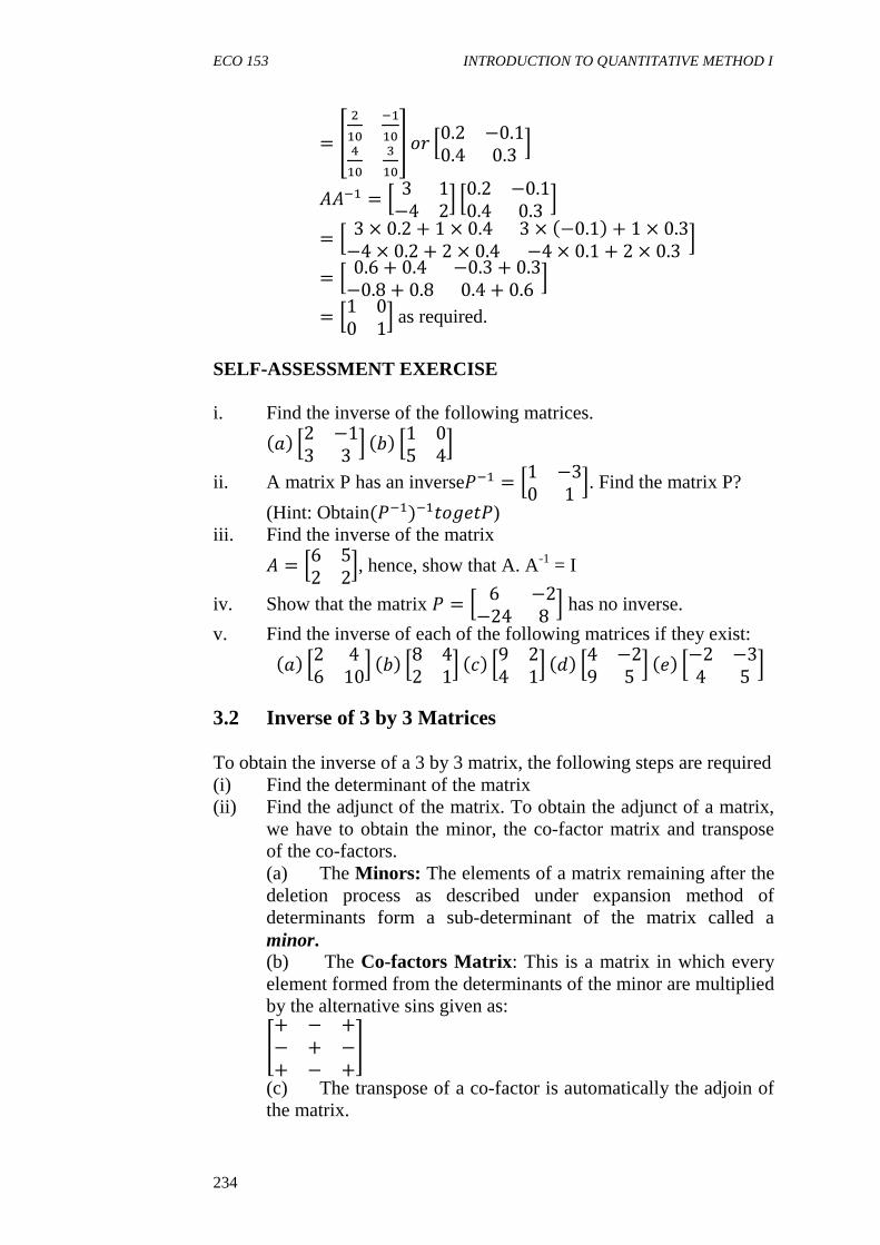
ECO 153 INTRODUCTION TO QUANTITATIVE METHOD I
234
= ! ��� ������� ���' L� �0.2 −0.10.4 0.3 �
���� = � 3 1−4 2� �0.2 −0.1
0.4 0.3 � = � 3 × 0.2 + 1 × 0.4 3 × >−0.1? + 1 × 0.3
−4 × 0.2 + 2 × 0.4 −4 × 0.1 + 2 × 0.3 � = � 0.6 + 0.4 −0.3 + 0.3
−0.8 + 0.8 0.4 + 0.6 �
= �1 00 1�as required.
SELF-ASSESSMENT EXERCISE i. Find the inverse of the following matrices. >�? �2 −1
3 3 � >"? �1 05 4�
ii. A matrix P has an inverseB�� = �1 −30 1 �. Find the matrix P?
(Hint: Obtain(B��)���L��B) iii. Find the inverse of the matrix
� = �6 52 2�, hence, show that A. A-1 = I
iv. Show that the matrix B = � 6 −2−24 8 � has no inverse.
v. Find the inverse of each of the following matrices if they exist: >�? �2 46 10� >"? �8 4
2 1� >#? �9 24 1� > ? �4 −2
9 5 � >? �−2 −34 5 �
3.2 Inverse of 3 by 3 Matrices
To obtain the inverse of a 3 by 3 matrix, the following steps are required (i) Find the determinant of the matrix (ii) Find the adjunct of the matrix. To obtain the adjunct of a matrix,
we have to obtain the minor, the co-factor matrix and transpose of the co-factors. (a) The Minors: The elements of a matrix remaining after the deletion process as described under expansion method of determinants form a sub-determinant of the matrix called a minor. (b) The Co-factors Matrix : This is a matrix in which every element formed from the determinants of the minor are multiplied by the alternative sins given as: �+ − +− + −+ − +
� (c) The transpose of a co-factor is automatically the adjoin of the matrix.
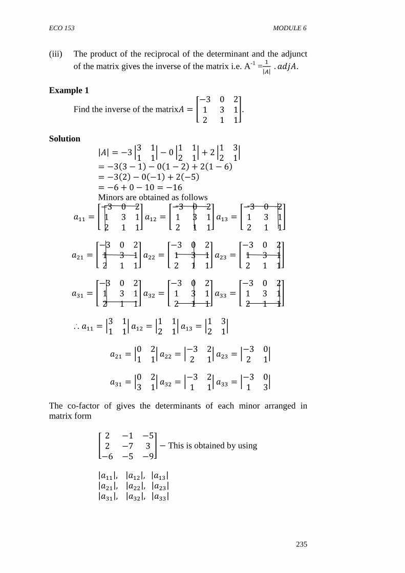
ECO 153 MODULE 6
235
(iii) The product of the reciprocal of the determinant and the adjunct
of the matrix gives the inverse of the matrix i.e. A-1 =�|�| .� K�.
Example 1
Find the inverse of the matrix� = �−3 0 21 3 12 1 1
�.
Solution
|�| = −3 D3 11 1D − 0 D1 1
2 1D + 2 D1 32 1D
= −3>3 − 1? − 0>1 − 2? + 2>1 − 6? = −3>2? − 0>−1? + 2>−5? = −6 + 0 − 10 = −16 Minors are obtained as follows ��� = �−3 0 2
1 3 12 1 1
� ��� = �−3 0 21 3 12 1 1
� ��� = �−3 0 21 3 12 1 1
� ��� = �−3 0 2
1 3 12 1 1
� ��� = �−3 0 21 3 12 1 1
� ��� = �−3 0 21 3 12 1 1
� ��� = �−3 0 2
1 3 12 1 1
� ��� = �−3 0 21 3 12 1 1
� ��� = �−3 0 21 3 12 1 1
�
... ��� = D3 11 1D ��� = D1 1
2 1D ��� = D1 32 1D
��� = D0 21 1D ��� = D−3 2
2 1D ��� = D−3 02 1D
��� = D0 23 1D ��� = D−3 2
1 1D ��� = D−3 01 3D
The co-factor of gives the determinants of each minor arranged in matrix form
� 2 −1 −52 −7 3−6 −5 −9
� − This is obtained by using
|���|,|���|,|���| |���|,|���|,|���| |���|,|���|,|���|
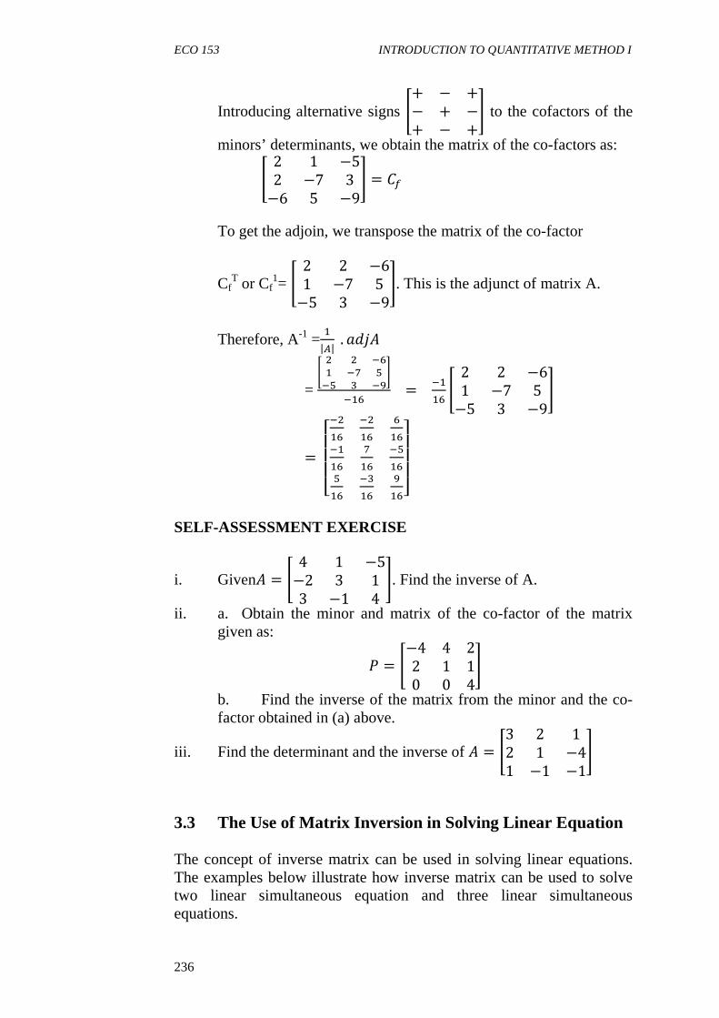
ECO 153 INTRODUCTION TO QUANTITATIVE METHOD I
236
Introducing alternative signs �+ − +− + −+ − +
� to the cofactors of the
minors’ determinants, we obtain the matrix of the co-factors as:
� 2 1 −52 −7 3−6 5 −9
� = ��
To get the adjoin, we transpose the matrix of the co-factor
CfT or Cf
1= � 2 2 −61 −7 5−5 3 −9
�. This is the adjunct of matrix A.
Therefore, A-1 =�|�| . � K�
= � � � ��� �� ��� � ������ = ���� � 2 2 −6
1 −7 5−5 3 −9
� = 23334
���� ���� ������� ��� ������� ���� ���67778
SELF-ASSESSMENT EXERCISE
i. Given� = � 4 1 −5−2 3 13 −1 4
�. Find the inverse of A.
ii. a. Obtain the minor and matrix of the co-factor of the matrix given as: B = �−4 4 2
2 1 10 0 4
� b. Find the inverse of the matrix from the minor and the co-factor obtained in (a) above.
iii. Find the determinant and the inverse of � = �3 2 12 1 −41 −1 −1
�
3.3 The Use of Matrix Inversion in Solving Linear Equation
The concept of inverse matrix can be used in solving linear equations. The examples below illustrate how inverse matrix can be used to solve two linear simultaneous equation and three linear simultaneous equations.

ECO 153 MODULE 6
237
Example Use inverse matrix to solve the unknown in each of the following pairs of simultaneous equations.
(1) 4x – y = 13 2x – 5y = -7
(2) Ajao bought 3 pens, 2 books and 4 pencils at ₦19. In the same market, Tola bought 6 pens, 2 books and a pencil at ₦37 while Oye bought 1 pen, 2 books and 3 pencils at ₦10. Required (a) Represent the information in a matrix system. (b) Use inverse method to obtain the unit price of a pen, a
book and a pencil.
Solution 1. 4x – y = 13
2x – 5y = -7 Writing in matrix form:
�4 −12 −5� ��%� = �13−7�
���
��%� = �������� ��� ��� ��%� = �4 −1
2 −5��� �13−7� Recall, (A-1) =
���|�|
D4 −12 −5D = >4 × 5? − >2 × −1?
= −20 − >−2? = −20 + 2 = −18
� K �4 −12 −5� = �−5 −1
−2 4 �
Hence, �4 −12 −5��� = �−5 −1
−2 4 � . ��� = !��� ������ ��'
�% = !��� ������ ��' �13−7�
� = �− �� × 13 + ��� × −7� = ����� − ��� = ����� = +4 % = ���� × 13 + �� × −7� = ����� − ��� = ����� = 3
... x = 4 and y = 3
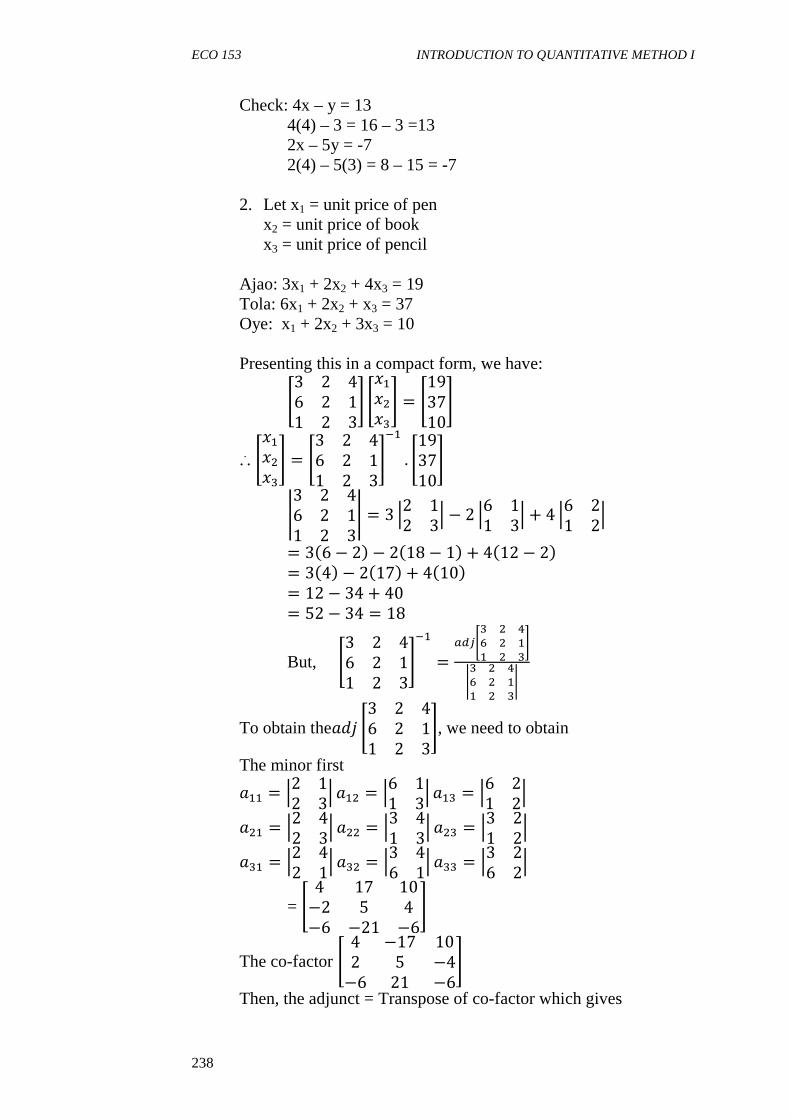
ECO 153 INTRODUCTION TO QUANTITATIVE METHOD I
238
Check: 4x – y = 13 4(4) – 3 = 16 – 3 =13 2x – 5y = -7 2(4) – 5(3) = 8 – 15 = -7 2. Let x1 = unit price of pen
x2 = unit price of book x3 = unit price of pencil
Ajao: 3x1 + 2x2 + 4x3 = 19 Tola: 6x1 + 2x2 + x3 = 37 Oye: x1 + 2x2 + 3x3 = 10 Presenting this in a compact form, we have:
�3 2 46 2 11 2 3
� �������� = �193710
�
... �������� = �3 2 46 2 11 2 3
��� . �193710
� E3 2 4
6 2 11 2 3
E = 3 D2 12 3D − 2 D6 1
1 3D + 4 D6 21 2D
= 3>6 − 2? − 2>18 − 1? + 4>12 − 2? = 3>4? − 2>17? + 4>10? = 12 − 34 + 40 = 52 − 34 = 18
But, �3 2 46 2 11 2 3
��� = ���� � �� � �� � ���� � �� � �� � ��
To obtain the� K �3 2 46 2 11 2 3
�, we need to obtain
The minor first ��� = D2 12 3D ��� = D6 1
1 3D ��� = D6 21 2D ��� = D2 4
2 3D ��� = D3 41 3D ��� = D3 2
1 2D ��� = D2 42 1D ��� = D3 4
6 1D ��� = D3 26 2D
= � 4 17 10−2 5 4−6 −21 −6
� The co-factor � 4 −17 10
2 5 −4−6 21 −6
�
Then, the adjunct = Transpose of co-factor which gives
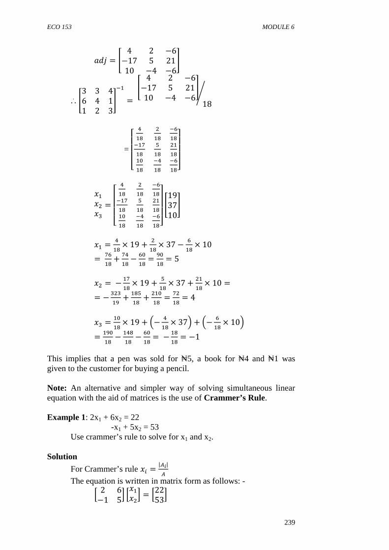
ECO 153 MODULE 6
239
� K = � 4 2 −6−17 5 2110 −4 −6
� ... �3 3 4
6 4 11 2 3
��� = � 4 2 −6−17 5 2110 −4 −6
�18
M
= 23334�� �� ������� �� ������ ��� ���67778
������ = 23334
�� �� ������� �� ������ ��� ���67778 �193710
�
�� = �� × 19 + �� × 37 − �� × 10
= ��� + ��� − ��� = ��� = 5
�� = − ��� × 19 + �� × 37 + ��� × 10 = = − ����� + ��� + ���� = ��� = 4
�� = ��� × 19 + N− �� × 37O + N− �� × 10O
= ���� − ��� − ��� = − �� = −1
This implies that a pen was sold for ₦5, a book for ₦4 and ₦1 was given to the customer for buying a pencil.
Note: An alternative and simpler way of solving simultaneous linear equation with the aid of matrices is the use of Crammer’s Rule.
Example 1: 2x1 + 6x2 = 22
-x1 + 5x2 = 53 Use crammer’s rule to solve for x1 and x2.
Solution
For Crammer’s rule �� = |��|�
The equation is written in matrix form as follows: -
� 2 6−1 5� ������ = �2253�
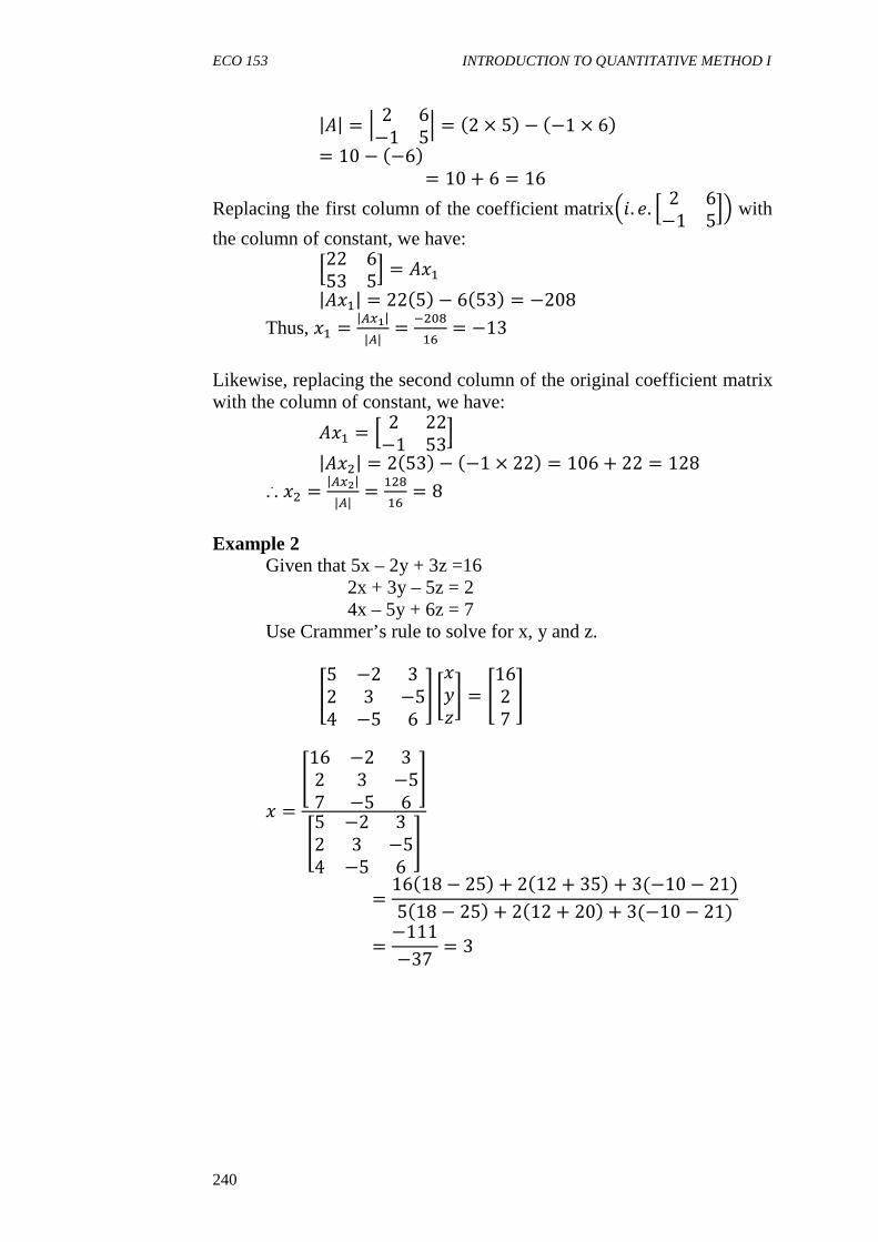
ECO 153 INTRODUCTION TO QUANTITATIVE METHOD I
240
|�| = D 2 6−1 5D = >2 × 5? − >−1 × 6?
= 10 − >−6? = 10 + 6 = 16
Replacing the first column of the coefficient matrixN�. . � 2 6−1 5�O with
the column of constant, we have:
�22 653 5� = ���
|���| = 22>5? − 6>53? = −208
Thus, �� = |���||�| = ����� = −13
Likewise, replacing the second column of the original coefficient matrix with the column of constant, we have:
��� = � 2 22−1 53�
|���| = 2>53? − >−1 × 22? = 106 + 22 = 128
... �� = |���||�| = ���� = 8
Example 2
Given that 5x – 2y + 3z =16 2x + 3y – 5z = 2 4x – 5y + 6z = 7 Use Crammer’s rule to solve for x, y and z.
�5 −2 32 3 −54 −5 6
� -�%$. = �1627
� � =
�16 −2 32 3 −57 −5 6
��5 −2 32 3 −54 −5 6
�= 16>18 − 25? + 2>12 + 35? + 3(−10 − 21)
5>18 − 25? + 2>12 + 20? + 3(−10 − 21)= −111
−37 = 3
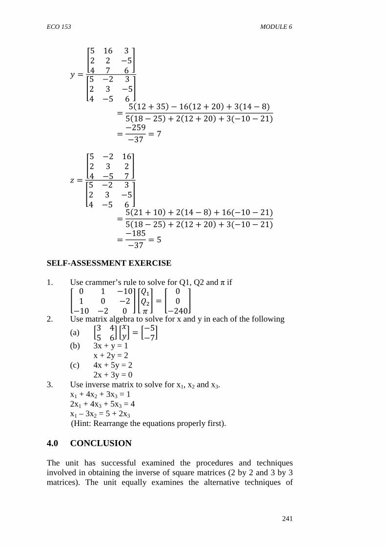
ECO 153 MODULE 6
241
% =�5 16 32 2 −54 7 6
��5 −2 32 3 −54 −5 6
�= 5>12 + 35? − 16>12 + 20? + 3(14 − 8)
5>18 − 25? + 2>12 + 20? + 3(−10 − 21)= −259
−37 = 7
$ =�5 −2 162 3 24 −5 7
��5 −2 32 3 −54 −5 6
�= 5>21 + 10? + 2>14 − 8? + 16(−10 − 21)
5>18 − 25? + 2>12 + 20? + 3(−10 − 21)= −185
−37 = 5
SELF-ASSESSMENT EXERCISE 1. Use crammer’s rule to solve for Q1, Q2 and π if � 0 1 −10
1 0 −2−10 −2 0
� �A�A�P � = � 00
−240�
2. Use matrix algebra to solve for x and y in each of the following
(a) �3 45 6� ��%� = �−5−7�
(b) 3x + y = 1 x + 2y = 2
(c) 4x + 5y = 2 2x + 3y = 0
3. Use inverse matrix to solve for x1, x2 and x3. x1 + 4x2 + 3x3 = 1 2x1 + 4x3 + 5x3 = 4 x1 – 3x2 = 5 + 2x3
(Hint: Rearrange the equations properly first). 4.0 CONCLUSION
The unit has successful examined the procedures and techniques involved in obtaining the inverse of square matrices (2 by 2 and 3 by 3 matrices). The unit equally examines the alternative techniques of
ECO 153 INTRODUCTION TO QUANTITATIVE METHOD I
242
solving linear equations (2 variables and 3 variables) using both matrix inversion as well as the Crammer’s rules. 5.0 SUMMARY
The inverse of a square matrix is mathematically given as the quotient of the adjoin of the matrix and the determinant of the matrix or the product of the adjoin of the matrix and the reciprocal of the determinant. ��� = � K�|�| = 1|�| × � K�
Simultaneous linear equations could be solved using matrix inversion and the Crammer’s rule. While the matrix inversion is a long process of solving linear equations, the Crammer’s rule is shorter and it employs only the concept of determinants. 6.0 TUTOR-MARKED ASSIGNMENT 1. Solve the following systems of linear equation using determinant
(Crammer’s rule). (a) 2x + 5y = 5 3x + 2y = 6
(b) x1 + x2 + x3 = 6 2x1 + x2 + x3 = 3
2x1 + 3x2 – 2x3 = 2 2. Use the matrix inverse to solve for x and y in each of the
following (a) 2x + 5y = 5 3x + 2y = 6 (b) 4x + 9y = 18 6x + 4y = 2 3. Solve for x, y and z using any approach of your choice.
3x1 - x2 – 2x3 = 2 2x2 – x3 = -1
6x1 – 5x2 = 3 (Hint: Rearrange the functional system first). 4. Use matrix inversion approach to solve for x, y and z.
2x + y + 2z = 1 -x + 4y + 2z = 0
3x + y + z = 2 5. Find, if it exists the inverse of each of the following
(a) �2 42 2� >"? �1 0
0 1� >#? �−2 15 −3�
(d) �3 25 4� >? �−4 6 8
2 1 71 5 9
�
ECO 153 MODULE 6
243
6. By method of co-factor expansion, find the inverse of � = �4 −3 02 2 −41 2 −2
� 7. Amina, Usman who is a merchant dealer in Yobe state deals in
three products namely Gold, Ball pen and Diamond. In her book of account were found sales for the month of August 2002 in the following order. 3 Gold, 5 Ball pens and 6 Diamond were sold at Damaturu. 5 Gold, 7 Ball pens and 4 Diamond were sold in Potiskum Total products sold at Gashua were in the ratio 1: 2: 2 for God, Ball pen and Diamond respectively.
If the sales in Damaturu summed up to N6, 000, that of Potiskum summed up to N7, 000and that of Gashua summed up to N6, 000.
Required (i) Present the information using matrix algebra. (ii) At what rate was each product sold.
8. The table below shows the number of hours required to make one of each of three products X, Y and Z in each of the three departments A, B and C. For example, it takes 1 hour of department A’s time, 2 hours of department B’s time and 3 hours of department C’s time to make I unit of product X. similar relation as shown for other entries
Department Hours to make 1 unit of product X Y Z
A 1 2 3 B 2 3 4 C 3 4 4
Hours available in department A, B and C are 140, 200 and 230 respectively. Required (i) Set up a system of linear equations available department are to be used (ii) Determine the product schedule using a matrix method.
ECO 153 INTRODUCTION TO QUANTITATIVE METHOD I
244
7.0 REFERENCES/FURHER READING Anthony, C. & Robert, D. (2006).Foundation Mathematics. (4th ed.).
London: Pearson Hall Publisher. Edward, T. D. (2004). Introduction to Mathematical Economics. (3rd
ed.). Delhi: Tata, Mc-Graw Hills Publishers. Elayn, Marton-Gay (2003). Introductory Algebra. (2nd ed.). New
Jersey: Prentice-Hall Inc. Hardwood, L. C. (1990). Ordinary Level Mathematics. Heinemann
Educational Books. Robert, S. & Geoff, B. (2008).Excellence in Mathematics for Senior
Secondary School. Ibadan: Macmillan Publishers Limited. Usman, A. S. (2005). Business Mathematics. Lagos: Apex Books
Limited.