Course on Model Predictive Control Part I – Introduction · Course on Model Predictive Control Part I – Introduction ... Brief history of Model Predictive Control Origins and

Course on Model Predictive ControlPart I – Introduction

Gabriele Pannocchia

Department of Chemical Engineering, University of Pisa, ItalyEmail: [email protected]

Facoltà di Ingegneria, Pisa.July 9th, 2012, Room A12

G. Pannocchia Course on Model Predictive Control. Part I – Introduction 1 / 33

Outline

1 Introduction to MPC: motivations and history

2 Comparison with conventional feedback control

3 Simple example and typical industrial architecture

4 Some reminders of linear systems theory and optimal control/estimation


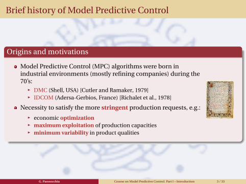
Brief history of Model Predictive Control

Origins and motivations

Model Predictive Control (MPC) algorithms were born inindustrial environments (mostly refining companies) during the70’s:

Ï DMC (Shell, USA) [Cutler and Ramaker, 1979]Ï IDCOM (Adersa-Gerbios, France) [Richalet et al., 1978]

Necessity to satisfy the more stringent production requests, e.g.:

Ï economic optimizationÏ maximum exploitation of production capacitiesÏ minimum variability in product qualities


Brief history of Model Predictive Control (cont’d)

Industry and academia

Nowadays, most complex plants especially in refining and(petro)chemical industries use MPC systems

After an initial reluctance, the academia “embraced” MPCcontributing to:

Ï establish theoretical foundationsÏ develop new algorithms


Commercial product evolution

Commercial Products (partial list updated to 1996)

[DMC] Dynamic Matrix Control ⇒ DMC Corporation (USA)

[SMCA] (ex IDCOM) Multivariable Control Architecture ⇒ Set-Point,Inc.(USA)

[PCT] (RMPCT) Predictive Control Technology ⇒ Honeywell - Profimatics(USA)

[OPC] Optimum Predictive Control ⇒ Treiber Controls, Inc. (Canada)

[MVPC] Multivariable Predictive Control ⇒ ABB Ind. System Corp. (USA)

[IDCOM-Y] ⇒ Johnson Yokogawa Corp. (USA)

[MVC] Multivariable Control ⇒ Continental Control, Inc. (USA)

[C-MCC] Contas-Multivariable Constrained Control ⇒ CONTAS s.r.l. (Italy)


Commercial product evolution

Merges

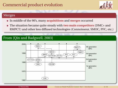
In middle of the 90’s, many acquisitions and merges occurred

The situation became quite steady with two main competitors (DMC+ andRMPCT) and other less diffused technologies (Connoisseur, SMOC, PFC, etc.)

From [Qin and Badgwell, 2003]

In recent years the MPC landscape has changeddrastically, with a large increase in the number ofreported applications, significant improvements intechnical capability, and mergers between several ofthe vendor companies. The primary purpose of thispaper is to present an updated, representative snapshotof commercially available MPC technology. The in-formation reported here was collected from vendorsstarting in mid-1999, reflecting the status of MPCpractice just prior to the new millennium, roughly 25years after the first applications.

A brief history of MPC technology development ispresented first, followed by the results of our industrialsurvey. Significant features of each offering are outlinedand discussed. MPC applications to date by each vendorare then summarized by application area. The finalsection presents a view of next-generation MPCtechnology, emphasizing potential business and researchopportunities.

2. A brief history of industrial MPC

This section presents an abbreviated history ofindustrial MPC technology. Fig. 1 shows an evolution-ary tree for the most significant industrial MPCalgorithms, illustrating their connections in a conciseway. Control algorithms are emphasized here becauserelatively little information is available on the develop-ment of industrial identification technology. The follow-ing sub-sections describe key algorithms on the MPCevolutionary tree.

2.1. LQG

The development of modern control concepts can betraced to the work of Kalman et al. in the early 1960s(Kalman, 1960a, b). A greatly simplified description oftheir results will be presented here as a reference pointfor the discussion to come. In the discrete-time context,

the process considered by Kalman and co-workers canbe described by a discrete-time, linear state-space model:

xk!1 " Axk ! Buk !Gwk; #1a$

yk " Cxk ! nk: #1b$

The vector u represents process inputs, or manipulatedvariables, and vector y describes measured processoutputs. The vector x represents process states to becontrolled. The state disturbance wk and measurementnoise nk are independent Gaussian noise with zeromean. The initial state x0 is assumed to be Gaussianwith non-zero mean.

The objective function F to be minimizedpenalizes expected values of squared input and statedeviations from the origin and includes separate stateand input weight matrices Q and R to allow for tuningtrade-offs:

F " E#J$; J "X

N

j"1

#jjxk!j jj2Q ! jjuk!j jj2R$: #2$

The norm terms in the objective function are defined asfollows:

jjxjj2Q " xTQx: #3$

Implicit in this formulation is the assumption that allvariables are written in terms of deviations from adesired steady state. It was found that the solution tothis problem, known as the linear quadratic Gaussian(LQG) controller, involves two separate steps. At timeinterval k; the output measurement yk is first used toobtain an optimal state estimate #xkjk:

#xkjk%1 " A #xk%1jk%1 ! Buk%1; #4a$

#xkjk " #xkjk%1 ! Kf #yk % C #xkjk%1$: #4b$

Then the optimal input uk is computed using an optimalproportional state controller:

uk " %Kc #xkjk: #5$

LQG

IDCOM-M HIECON

SMCAPCTPFC

IDCOM

SMOC

Connoisseur

DMC

DMC+

QDMC

RMPC

RMPCT

1960

1970

1980

1990

2000

1st generationMPC

2nd generationMPC

3rd generationMPC

4th generationMPC

Fig. 1. Approximate genealogy of linear MPC algorithms.

S.J. Qin, T.A. Badgwell / Control Engineering Practice 11 (2003) 733–764734


Keywords

MPC keywords

In most commercial product acronyms we find several important keywords thatdefine the MPC technologies

Control

Model

Predictive

Multivariable

Robustness

Constraints

Optimization

Identification

Analysis of such characteristic features in comparison with conventional controlschemes


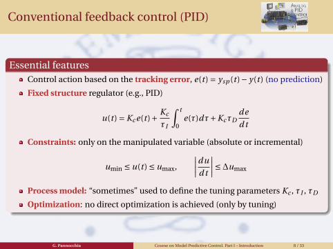
Conventional feedback control (PID)

Essential featuresControl action based on the tracking error, e(t ) = ysp (t )− y(t ) (no prediction)

Fixed structure regulator (e.g., PID)

u(t ) = Kc e(t )+ Kc

τI

∫ t

0e(τ)dτ+KcτD

de

d t

Constraints: only on the manipulated variable (absolute or incremental)

umin ≤ u(t ) ≤ umax,

∣∣∣∣du

d t

∣∣∣∣≤∆umax

Process model: “sometimes” used to define the tuning parameters Kc , τI , τD

Optimization: no direct optimization is achieved (only by tuning)


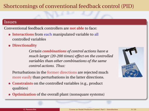
Shortcomings of conventional feedback control (PID)

IssuesConventional feedback controllers are not able to face:

Interactions from each manipulated variable to allcontrolled variables

Directionality

Certain combinations of control actions have amuch larger (20-200 times) effect on the controlledvariables than other combinations of the samecontrol actions. Thus:

Perturbations in the former directions are rejected muchmore easily than perturbations in the latter directions.

Constraints on the controlled variables (e.g., productqualities)

Optimization of the overall plant (nonsquare systems)


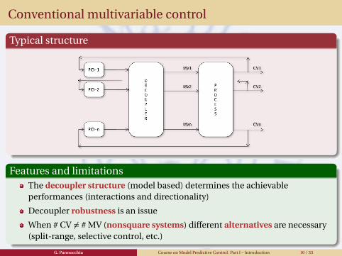
Conventional multivariable control

Typical structure

Features and limitationsThe decoupler structure (model based) determines the achievableperformances (interactions and directionality)

Decoupler robustness is an issue

When # CV 6= # MV (nonsquare systems) different alternatives are necessary(split-range, selective control, etc.)


Main features of MPC

MPC became a successful technology due to the following features:

ease of handling multivariable systems

ease of handling complicated dynamics (e.g., delays, inverseresponse, ramps, etc.)

ease of handling constraints on controlled and manipulatedvariables (pushing the plant towards its limits)

straightforward applicability to feedforward information(measurable disturbances)


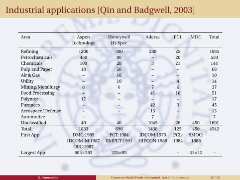
Industrial applications [Qin and Badgwell, 2003]

Area Aspen Honeywell Adersa PCL MDC TotalTechnology Hi-Spec

Refining 1200 480 280 25 1985Petrochemicals 450 80 – 20 550Chemicals 100 20 3 21 144Pulp and Paper 18 50 – – 68Air & Gas – 10 – – 10Utility – 10 – 4 14Mining/Metallurgy 8 6 7 6 37Food Processing – – 41 10 51Polymer 17 – – – 17Furnaces – – 42 3 45Aerospace/Defense – – 13 – 13Automotive – – 7 – 7Unclassified 40 40 1045 26 450 1601Total 1833 696 1438 125 450 4542First App. DMC:1985 PCT:1984 IDCOM:1973 PCL: SMOC:

IDCOM-M:1987 RMPCT:1991 HIECON:1986 1984 1988OPC:1987

Largest App 603×283 225×85 – 31×12 –


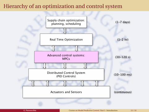
Hierarchy of an optimization and control system


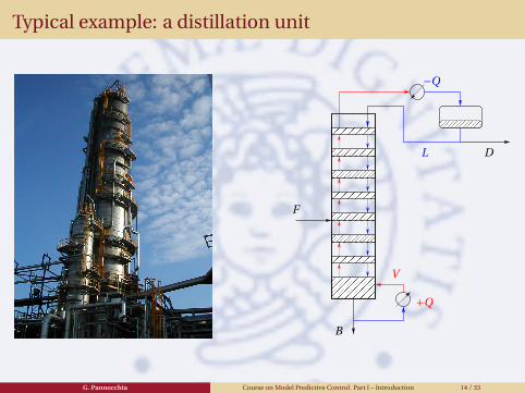
Typical example: a distillation unit

��

��

��

��

��

��

��

��

��

��

DL

V

B

F

−Q

+Q


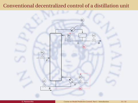
Conventional decentralized control of a distillation unit

FC

AC

AC

FC LC

PC

LC

FC

L

B

D

V

F


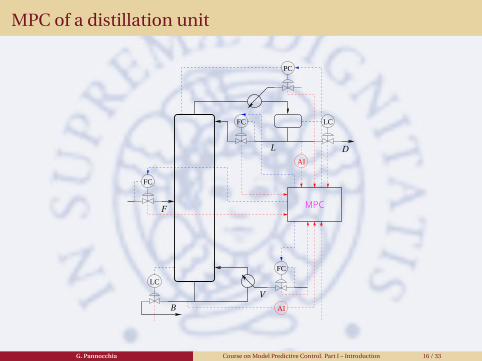
MPC of a distillation unit

FC

FC LC

PC

LC

FC

AI

AI

L

B

D

V

F MPC


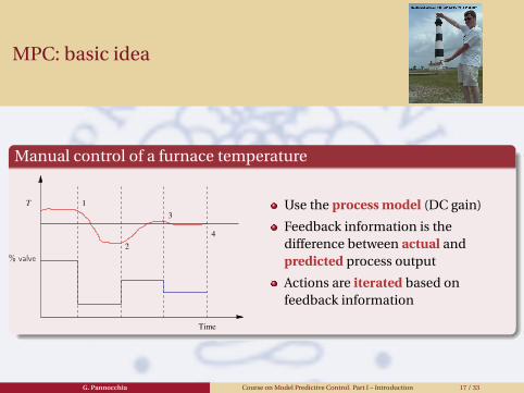
MPC: basic idea

Manual control of a furnace temperature

4

Time

1

2

3

T

% valve

Use the process model (DC gain)

Feedback information is thedifference between actual andpredicted process output

Actions are iterated based onfeedback information


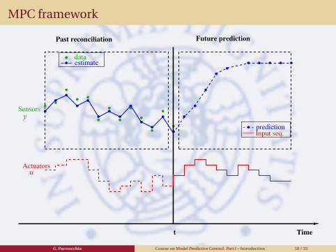
MPC framework

Timet

Past reconciliation

Sensors

estimatedata

predictionInput seq.

Future prediction

Actuators

y

u


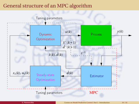
General structure of an MPC algorithm

MPC

ProcessDynamic

Steady-state

u(k)

Optimization

Estimatord̂(k)

Optimization

Tuning parameters

Tuning parameters

x̂(k), d̂(k)

xs(k), us(k)

z−1

x̂−(k +1)d̂−(k +1)

y(k)


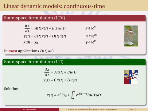
Linear dynamic models: continuous-time

State-space formulation (LTV)

d x

d t= A(t )x(t )+B(t )u(t ) x ∈Rn

y(t ) =C (t )x(t )+D(t )u(t ) u ∈Rm

x(0) = x0 y ∈Rp

In most applications D(t ) = 0

State-space formulation (LTI)

d x

d t= Ax(t )+Bu(t )

y(t ) =C x(t )+Du(t )

Solution:

x(t ) = e At x0 +∫ t

0e A(t−τ)Bu(τ)dτ


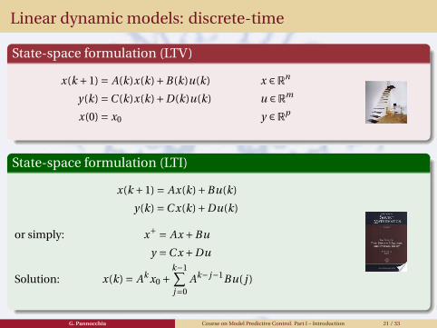
Linear dynamic models: discrete-time

State-space formulation (LTV)

x(k +1) = A(k)x(k)+B(k)u(k) x ∈Rn

y(k) =C (k)x(k)+D(k)u(k) u ∈Rm

x(0) = x0 y ∈Rp

State-space formulation (LTI)

x(k +1) = Ax(k)+Bu(k)

y(k) =C x(k)+Du(k)

or simply: x+ = Ax +Bu

y =C x +Du

Solution: x(k) = Ak x0 +k−1∑j=0

Ak− j−1Bu( j )


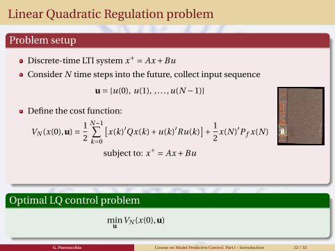
Linear Quadratic Regulation problem

Problem setup

Discrete-time LTI system x+ = Ax +Bu

Consider N time steps into the future, collect input sequence

u = {u(0), u(1), , . . . ,u(N −1)}

Define the cost function:

VN (x(0),u) = 1

2

N−1∑k=0

[x(k)′Qx(k)+u(k)′Ru(k)

]+ 1

2x(N )′P f x(N )

subject to: x+ = Ax +Bu

Optimal LQ control problem

minu

VN (x(0),u)


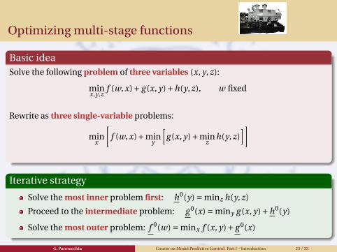
Optimizing multi-stage functions

Basic ideaSolve the following problem of three variables (x, y, z):

minx,y,z

f (w, x)+ g (x, y)+h(y, z), w fixed

Rewrite as three single-variable problems:

minx

[f (w, x)+min

y

[g (x, y)+min

zh(y, z)

]]

Iterative strategy

Solve the most inner problem first: h0(y) = minz h(y, z)

Proceed to the intermediate problem: g 0(x) = miny g (x, y)+h0(y)

Solve the most outer problem: f 0(w) = minx f (x, y)+ g 0(x)


Dynamic programming solution of the LQR problem

Principle of dynamic programming applied to LQR problem

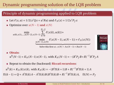
Let `(x,u) = 1/2(x ′Qx +u′Ru) and `N (x) = 1/2x ′P f x

Optimize over u(N −1) and x(N )

minu(0),x(1),...,u(N−2),x(N−1)

N−2∑k=0

`(x(k),u(k))+

minu(N−1),x(N )

`(x(N −1),u(N −1))+`N (x(N ))︸︷︷︸Solve this first s.t. x(N ) = Ax(N −1)+Bu(N −1)

Obtain:

u0(N−1) = KN (N−1)x(N−1), with KN (N−1) =−(B ′P f B+R)−1B ′P f A

Repeat to obtain the (backward) Riccati recursions:

u0(k) = KN (k)x(k), with KN (k) =−(B ′Π(k +1)B +R)−1B ′Π(k +1)A

Π(k −1) =Q + A′Π(k)A− A′Π(k)B(B ′Π(k)B +R)−1B ′Π(k)A, Π(N ) = P f


Infinite horizon LQR problem

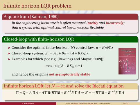
A quote from [Kalman, 1960]

In the engineering literature it is often assumed (tacitly and incorrectly)that a system with optimal control law is necessarily stable.

Closed-loop with finite-horizon LQR

Consider the optimal finite-horizon (N ) control law: u = KN (0)x

Closed-loop system: x+ = Ax +Bu = (A+BKN )x

Examples for which (see e.g. [Rawlings and Mayne, 2009]):

max |eig(A+BKN )| ≥ 1

and hence the origin is not asymptotically stable

Infinite horizon LQR: let N →∞ and solve the Riccati equation

Π=Q + A′ΠA− A′ΠB(B ′ΠB +R)−1B ′ΠA ⇒ K =−(B ′ΠB +R)−1B ′ΠA


Controllability

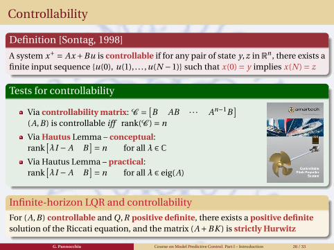
Definition [Sontag, 1998]

A system x+ = Ax +Bu is controllable if for any pair of state y, z in Rn , there exists afinite input sequence {u(0), u(1), . . . ,u(N −1)} such that x(0) = y implies x(N ) = z

Tests for controllability

Via controllability matrix: C = [B AB · · · An−1B

](A,B) is controllable iff rank(C ) = n

Via Hautus Lemma – conceptual:rank

[λI − A B

]= n for all λ ∈CVia Hautus Lemma – practical:rank

[λI − A B

]= n for all λ ∈ eig(A)

Infinite-horizon LQR and controllability

For (A,B) controllable and Q,R positive definite, there exists a positive definitesolution of the Riccati equation, and the matrix (A+BK ) is strictly Hurwitz


Stochastic linear systems

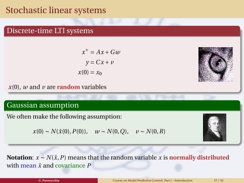
Discrete-time LTI systems

x+ = Ax +Gw

y =C x + v

x(0) = x0

x(0), w and v are random variables

Gaussian assumption

We often make the following assumption:

x(0) ∼ N (x̄(0),P (0)), w ∼ N (0,Q), v ∼ N (0,R)

Notation: x ∼ N (x̄,P ) means that the random variable x is normally distributedwith mean x̄ and covariance P


Linear optimal state estimation

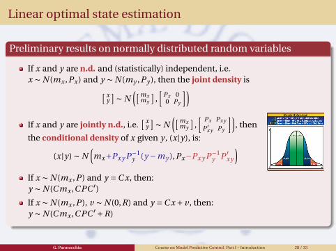
Preliminary results on normally distributed random variables

If x and y are n.d. and (statistically) independent, i.e.x ∼ N (mx ,Px ) and y ∼ N (my ,Py ), then the joint density is[ x

y]∼ N

([mxmy

],[

Px 00 Py

])If x and y are jointly n.d., i.e.

[ xy]∼ N

([mxmy

],[ Px Px y

P ′x y Py

]), then

the conditional density of x given y , (x|y), is:

(x|y) ∼ N(mx+Px y P−1

y (y −my ),Px−Px y P−1y P ′

x y

)If x ∼ N (mx ,P ) and y =C x, then:y ∼ N (C mx ,C PC ′)If x ∼ N (mx ,P ), v ∼ N (0,R) and y =C x + v , then:y ∼ N (C mx ,C PC ′+R)


Linear optimal state estimation (cont.’d)

Deriving the Kalman filter...

Assume prior knowledge: x(k) ∼ N (x̂−(k),P−(k))

Obtain measurement y(k) that satisfies:[

x(k)y(k)

]= [

I 0C I

][x(k)v(k)

]Since x(k) and v(k) are independent, there holds:[

x(k)y(k)

]∼ N

([x̂−(k)

C x̂−(k)

],[

P−(k) P−(k)C ′C P−(k) C P−(k)C ′+R

])Conditional density (x(k)|y(k)) ∼ N (x̂(k),P (k)) with:x̂(k) = x̂−(k)+L(k)

(y(k)−C x̂−(k)

)L(k) = P−(k)C ′(C P−(k)C ′+R)−1

P (k) = P−(k)−P−(k)C ′(C P−(k)C ′+R)−1P−(k)C ′

Forecast using x(k +1) = Ax(k)+Gw(k)

x(k +1) ∼ N ( Ax̂(k)︸︷︷︸x̂−(k+1)

, AP (k)A′+GQG ′︸︷︷︸P−(k+1)

)


Linear optimal state estimation (cont.’d)

Convergence of the state estimator

Consider the noise-free system:

x(k +1) = Ax(k)+Bu(k), y =C x(k)

Given an incorrect initial estimate x̂−(0), we use a time-varyingKalman filter L(k). Is x̂−(k) → x(k) as k →∞?

Estimation error and steady-state Kalman filter

Define the state estimation error: e(k) = x(k)− x̂−(k)

We obtain:e(k +1) = (A− AL(k)C )e(k)

Thus, e(k) → 0 as k →∞ if (A− ALC ) is strictly Hurwitz, where:L =ΠC ′(CΠC ′+R)−1

Π= AΠA′− AΠC ′(CΠC ′+R)−1ΠC ′A′+GQG ′


Observability

Definition [Sontag, 1998]

A system x+ = Ax +Bu with measured output y =C x, is observable if there exists afinite N such that for any (unknown) initial state x(0) and N measurements{y(0), y(1), . . . , y(N −1)}, the initial state x(0) can be determined uniquely

Tests for observability

Via observability matrix: O = C

C A...

C An−1

(A,C ) is observable iff rank(O ) = n

Via Hautus Lemma – conceptual:

rank

[λI − A

C

]= n for all λ ∈C

Via Hautus Lemma – practical:

rank

[λI − A

C

]= n for all λ ∈ eig(A)


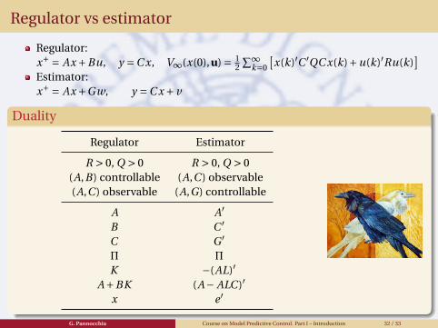
Regulator vs estimator

Regulator:x+ = Ax +Bu, y =C x, V∞(x(0),u) = 1

2

∑∞k=0

[x(k)′C ′QC x(k)+u(k)′Ru(k)

]Estimator:x+ = Ax +Gw, y =C x + v

Duality

Regulator Estimator

R > 0, Q > 0 R > 0, Q > 0(A,B) controllable (A,C ) observable(A,C ) observable (A,G) controllable

A A′B C ′C G ′Π Π

K −(AL)′A+BK (A− ALC )′

x e ′


References

C. R. Cutler and B. L. Ramaker. Dynamic matrix control – a computer algorithm. In AIChE 86th NationalMeeting, Houston, TX, 1979.

R. E. Kalman. Contributions to the theory of optimal control. Bull. Soc. Math. Mex., 5:102–119, 1960.

S. J. Qin and T. A. Badgwell. A survey of industrial model predictive control technology. Cont. Eng.Practice, 11:733–764, 2003.

J. B. Rawlings and D. Q. Mayne. Model Predictive Control: Theory and Design. Nob Hill Publishing,Madison, WI, 2009.

J. Richalet, J. Rault, J. L. Testud, and J. Papon. Model predictive heuristic control: applications toindustrial processes. Automatica, 14:413–1554, 1978.

E. D. Sontag. Mathematical Control Theory. Springer, 1998.


Documents

Course on Model Predictive Control Part I – Introduction · Course on Model Predictive Control Part I – Introduction ... Brief history of Model Predictive Control Origins and