Course Information Text: Special reprint of Applied …web.ics.purdue.edu/~wsharaba/stat512/lecture1.pdfStatistics 512: Applied Regression Analysis Professor Sharabati Purdue University

Statistics 512: Applied Regression AnalysisProfessor Sharabati

Purdue UniversityFall 2014

Course Information

Text: Special reprint of Applied Linear Statistical Models,

5th edition by Kutner, Neter, Nachtsheim, and Li, 2012.

Recommended: Applied Statistics and the SAS

Programming Language, 5th edition by Cody and Smith.

Page 1 August 22, 2014Page 1



Professor: Walid Sharabati, HAAS 112.

Office Hours: MW 2:30pm-3:20pm, TTh 10:30-11:00

am, or by appointment, or e-mail

[email protected]

Evaluation: Problem sets will be assigned (more or

less) weekly. They will typically be due on Thursday or

Friday. Refer to the handout about specific evaluation

policies.




Lecture Notes

• Available as PDF

• Usually (hopefully) prepared a week in advance

• Not comprehensive (Be prepared to take notes.)

• One chapter per week

• Ask questions if you’re confused




Webpage

http://www.stat.purdue.edu/∼wsharaba/stat512.htm

• Announcements

• Lecture Notes

• Homework Assignments

• Data Sets and SAS files

• General handouts

– Course Information

– Calendar




Mailing List

I will very occasionally send reminders or

announcements through e-mail.

Blackboard Learn

• Holds solutions documents

• Moniter grades

• Information restricted to enrolled students

• Discussion groups




Statistics 512: Applied Regression Analysis

Overview

We will cover

• simple linear regression

• multiple regression

• analysis of variance (ANOVA)




Emphasis will be placed on using selected practical tools

(such as SAS) rather than on mathematical

manipulations. We want to understand the theory so that

we can apply it appropriately. Some of the material on

SLR will be review, but our goal with SLR is to be able to

generalize the methods to MLR.




SAS is the program we will use to perform data analysis for this

class. Learning to use SAS will be a large part of the course.

Getting Help with SAS

Several sources for help:

• SAS Help Files (not always best)

• World Wide Web (look up the syntax in your favorite search

engine)

• SAS Getting Started (in SAS Files section of class website)

and Tutorials

• Statistical Consulting Service




• Evening Help Sessions

• Applied Statistics and the SAS Programming Language, 5th

edition by Cody and Smith; most relevant material in Chapters 1,

2, 5, 7, and 9.

• Your instructor

Statistical Consulting Service

Math B5 Hours 10-4 M through F

http://www.stat.purdue.edu/scs/




I will often give examples from SAS in class. The programs used in

lecture (and any other programs you should need) will be available

for you to download from the website.

I will usually have to edit the output somewhat to get it to fit on the

page of notes. You should run the SAS programs yourself to see the

real output and experiment with changing the commands to learn

how they work. Let me know if you get confused about what is input,

output, or my comments. I will tell you the names of all SAS files I

use in these notes. If the notes differ from the SAS file, take the

SAS file to be correct, since there may be cut-and-paste errors.

There is a tutorial in SAS to hep you get started.

Help→ Getting Started with SAS Software




You should spend some time before next week getting comfortable

with SAS (see HW #0).

For today, don’t worry about the detailed syntax of the commands.

Just try to get a sense of what is going on.




Example (Price Analysis for Diamond Rings in Singapore)

Variables

• response variable – price in Singapore dollars (Y )

• explanatory variable – weight of diamond in carats (X)

Goals

• Create a scatterplot

• Fit a regression line

• Predict the price of a sale for a 0.43 carat diamond ring




SAS Data Step

File diamond.sas on website.

One way to input data in SAS is to type or paste it in. In this

case, we have a sequence of ordered pairs (weight, price).

data diamonds;

input weight price @@;

cards;

.17 355 .16 328 .17 350 .18 325 .25 642 .16 342 .15 322 .19 485

.21 483 .15 323 .18 462 .28 823 .16 336 .20 498 .23 595 .29 860

.12 223 .26 663 .25 750 .27 720 .18 468 .16 345 .17 352 .16 332

.17 353 .18 438 .17 318 .18 419 .17 346 .15 315 .17 350 .32 918

.32 919 .15 298 .16 339 .16 338 .23 595 .23 553 .17 345 .33 945

.25 655 .35 1086 .18 443 .25 678 .25 675 .15 287 .26 693 .15 316

.43 .

;




data diamonds1;

set diamonds;

if price ne .;

Syntax Notes

• Each line must end with a semi-colon.

• There is no output from this statement, but information does

appear in the logwindow.

• Often you will obtain data from an existing SAS file or import it

from another file, such as a spreadsheet. Examples showing

how to do this will come later.




SAS proc print

Now we want to see what the data look like.

proc print data=diamonds;

run;

Obs weight price

1 0.17 355

2 0.16 328

3 0.17 350

...

47 0.26 693

48 0.15 316

49 0.43 .




We want to plot the data as a scatterplot, using circles to

represent data points and adding a curve to see if it

looks linear. The symbol statement “v = circle ”

(v stands for “value”) lets us do this. The symbol

statement “i = sm70 ” will add a smooth line using

splines (interpolation = smooth). These are options

which stay on until you turn them off. In order for the

smoothing to work properly, we need to sort the data by

the X variable.




proc sort data=diamonds1; by weight;

symbol1 v=circle i=sm70;

title1 ’Diamond Ring Price Study’;

title2 ’Scatter plot of Price vs. Weight with Smoothing Curve’;

axis1 label=(’Weight (Carats)’);

axis2 label=(angle=90 ’Price (Singapore $$)’);

proc gplot data=diamonds1;

plot price*weight / haxis=axis1 vaxis=axis2;

run;







Now we want to use the simple linear regression to fit a line throughthe data. We use the symbol option “i = rl ”, meaning“interpolation = regression line” (that’s an “L”, not a one).

symbol1 v=circle i=rl;

title2 ’Scatter plot of Price vs. Weight with Regression Line’;

proc gplot data=diamonds1;

plot price*weight / haxis=axis1 vaxis=axis2;

run;







We use proc reg (regression) to estimate aregression line and calculate predictors and residualsfrom the straight line. We tell it what the data are, whatthe model is, and what options we want.proc reg data=diamonds; model price=weight/clb p r;

output out=diag p=pred r=resid;

id weight; run;

Analysis of Variance

Sum of Mean

Source DF Squares Square F Value Pr > F

Model 1 2098596 2098596 2069.99 <.0001

Error 46 46636 1013.81886

Corrected Total 47 2145232

Root MSE 31.84052 R-Square 0.9783

Dependent Mean 500.08333 Adj R-Sq 0.9778

Coeff Var 6.36704




Parameter Estimates

Parameter Standard

Variable DF Estimate Error t Value Pr > |t|

Intercept 1 -259.62591 17.31886 -14.99 <.0001

weight 1 3721.02485 81.78588 45.50 <.0001




proc print data=diag;

run;

. Output Statistics

Dep Var Predicted Std Error Std Error

Obs weight price Value Mean Predict Residual Residual

1 0.17 355.0000 372.9483 5.3786 -17.9483 31.383

2 0.16 328.0000 335.7381 5.8454 -7.7381 31.299

3 0.17 350.0000 372.9483 5.3786 -22.9483 31.383

4 0.18 325.0000 410.1586 5.0028 -85.1586 31.445

5 0.25 642.0000 670.6303 5.9307 -28.6303 31.283

...

46 0.15 287.0000 298.5278 6.3833 -11.5278 31.194

47 0.26 693.0000 707.8406 6.4787 -14.8406 31.174

48 0.15 316.0000 298.5278 6.3833 17.4722 31.194




Simple Linear Regression

Why Use It?

• Descriptive purposes (cause/effect relationships)

• Control (often of cost)

• Prediction of outcomes




Data for Simple Linear Regression

• Observe i = 1, 2, . . . , n pairs of variables

(explanatory, response)

• Each pair often called a case or a data point

• Yi = ith response

• Xi = ith explanatory variable




Simple Linear Regression Model

Yi = β0 + β1Xi + εi for i = 1, 2, . . . , n

Simple Linear Regression Model Parameters

• β0 is the intercept.

• β1 is the slope.

• εi are independent, normally distributed random errors with

mean 0 and variance σ2, i.e.,

εi ∼ N(0, σ2)




Features of Simple Linear Regression Model

• Individual Observations: Yi = β0 + β1Xi + εi

• Since εi are random, Yi are also random and

E(Yi) = β0 + β1Xi + E(εi) = β0 + β1Xi

Var(Yi) = 0 + Var(εi) = σ2.

Since εi is Normally distributed,

Yi ∼ N(β0 + β1Xi, σ2) (See A.4, page 1302)




Fitted Regression Equation and Residuals

We must estimate the parameters β0, β1, σ2 from the

data. The estimates are denoted b0, b1, s2. These give

us the fitted or estimated regression line

Yi = b0 + b1Xi, where

• b0 is the estimated intercept.

• b1 is the estimated slope.

• Yi is the estimated mean for Y , when the predictor is

Xi (i.e., the point on the fitted line).




• ei is the residual for the ith case (the vertical distance

from the data point to the fitted regression line). Note

that ei = Yi − Yi = Yi − (b0 + b1Xi).




Using SAS to Plot the Residuals (Diamond Example)

When we called proc regearlier, we assigned theresiduals to the name “resid ” and placed them in anew data set called “diag ”. We now plot them vs. X .

proc gplot data=diag;

plot resid*weight / haxis=axis1 vaxis=axis2 vref=0;

where price ne .;

run;




Notice there does not appear to be any obvious pattern in the

residuals. We’ll talk a lot more about diagnostics later, but for now,

you should know that looking at residuals plots is an important way

to check assumptions.




Least Squares

• Want to find “best” estimators b0 and b1.

• Will minimize the sum of the squared residuals∑ni=1 e2

i =∑n

i=1(Yi − (b0 + b1Xi))2.

• Use calculus: take derivative with respect to b0 and

with respect to b1 and then set the two result

equations equal to zero and solve for b0 and b1 (see

KNNL, pages 17-18).




Least Squares Solution

• These are the best estimates for β1 and β0.

b1 =

∑(Xi − X)(Yi − Y )∑

(Xi − X)2=

SSXY

SSX

b0 = Y − b1X

• These are also maximum likelihood estimators (MLE), see

KNNL, pages 26-32.

• This estimate is the “best” because because it is unbiased (its

expected value is equal to the true value) with minimum

variance.




Maximum Likelihood

Yi ∼ N(β0 + β1Xi, σ2)

fi =1√

2πσ2e−

12(

Yi−β0−β1Xiσ )

2

L = f1 × f2 × . . .× fn – likelihood function

Find values for β0 and β1 which maximize L. These are

the SAME as the least squares estimators b0 and b1!!!




Estimation of σ2

We also need to estimate σ2 with s2. We use the sum of squared

residuals, SSE, divided by the degrees of freedom n− 2.

s2 =

∑(Yi − Yi)

2

n− 2=

∑e2

i

n− 2

=SSE

dfE

= MSE

s =√

s2 = Root MSE,

where SSE =∑

e2i is the sum of squared residuals or “errors”,

and MSE stands for “mean squared error”.




There will be other estimated variance for other

quantities, and these will also be denoted s2, e.g.

s2{b1}. Without any {}, s2 refers to the value above –

that is, the estimated variance of the residuals.




Identifying these things in the SAS output


Sum of Mean


Model 1 2098596 2098596 2069.99 <.0001

Error 46 46636 1013.81886


Root MSE 31.84052 R-Square 0.9783

Dependent Mean 500.08333 Adj R-Sq 0.9778

Coeff Var 6.36704

Parameter Estimates

Parameter Standard

Variable DF Estimate Error t Value Pr > |t| 95% Confidence Limits

Intercept 1 -259.62591 17.31886 -14.99 <.0001 -294.48696 -224.76486

weight 1 3721.02485 81.78588 45.50 <.0001 3556.39841 3885.65129




Review of Statistical Inference for Normal Samples

This should be review!

In Statistics 503/511 you learned how to construct

confidence intervals and do hypothesis tests for the

mean of a normal distribution, based on a random

sample. Suppose we have an iid (random) sample

W1, . . . , Wn from a normal distribution. (Usually, I

would use the symbol X or Y , but I want to keep the

context general and not use the symbols we use for

regression.)




We have

Wi ∼iid N(µ, σ2) where µ and σ2 are unknown

W =

∑Wi

n= sample mean

SSW =∑

(Wi − W )2 = sum of squares for W

s2{W} =

∑(Wi − W )2

n− 1=

SSW

n− 1= sample variance

s{W} =√

s2{W} = sample standard deviation

s{W} =s{W}√

n= standard error of the mean




and from these definitions, we obtain

W ∼ N

(µ,

σ2

n

),

T =W − µ

s{W} has a t-distribution with n− 1 df (in short, T ∼ tn−1)

This leads to inference:

• confidence intervals for µ

• significance tests for µ.




Confidence Intervals

We are 100(1− α)% confident that the following

interval contains µ:

W ± tcs{W} =[W − tcs{W}, W + tcs{W}]

where tc = tn−1(1− α2 ), the upper (1− α

2 ) percentile

of the t distribution with n− 1 degrees of freedom, and

1− α is the confidence level (e.g. 0.95 = 95%, so

α = 0.05).




Significance Tests

To test whether µ has a specific value, we use a t-test

(one sample, non-directional).

H0 : µ = µ0 vs Ha : µ 6= µ0

• t = W−µ0

s{W} has a tn−1 distribution under H0.

• Reject H0 if |t| ≥ tc, where tc = tn−1(1− α2 ).

• p-value = ProbH0(|T | > |t|), where T ∼ tn−1.




The p-value is twice the area in the upper tail of the tn−1

distribution above the observed |t|. It is the probability of

observing a test statistic at least as extreme as what was

actually observed, when the null hypothesis is really true.

We reject H0 if p ≤ α. (Note that this is basically the

same – more general, actually – as having |t| ≥ tc.)




Important Notational Comment

The text says “conclude HA” if t is in the rejection region

(|t| ≥ tc), otherwise “conclude H0”. This is shorthand for

• “conclude HA” means “there is sufficient evidence in

the data to conclude that H0 is false, and so we

assume that HA is true.”

• “conclude H0” means “there is insufficient evidence in

the data to conclude that either H0 or HA is true or

false, so we default to assuming that H0 is true.”




Notice that a failure to reject H0 does

not mean that there was any evidence

in favor of H0

NOTE: In this course, α = 0.05 unless otherwise specified.




Section 2.1: Inference about β1

b1 ∼ N(β1, σ2{b1})

where σ2{b1} =σ2

SSX

t =(b1 − β1)

s{b1}

where s{b1} =

√s2

SSX

t ∼ tn−2 if β1 = 0




According to our discussion above for “W ”, you

therefore know how to obtain CI’s and t-tests for β1. (I’ll

go through it now but not in the future.) There is one

important difference: the degrees of freedom (df) here

are n− 2, not n− 1, because we are also estimating

β0.




Confidence Interval for β1

• b1 ± tcs{b1},

• where tc = tn−2(1− α2), the upper 100(1− α

2) percentile of

the t distribution with n− 2 degrees of freedom

• 1− α is the confidence level.

Significance Tests for β1

• H0 : β1 = 0 vs Ha : β1 6= 0

• t = b1−0s{b1}

• Reject H0 if |t| ≥ tc, tc = tn−2(1− α/2)




• p-value = Prob(|T | > |t|), where T ∼ tn−2




Inference for β0

• b0 ∼ N(β0, σ2{b0}) where

σ2{b0} = σ2[

1n + X2

SSX

].

• t = b0−β0

s{b0} for s{b0} replacing σ2 by s2 and take√

• s{b0} = s√

1n + X2

SSX

• t ∼ tn−2




Confidence Interval for β0

• b0 ± tcs{b0}• where tc = tn−2(1− α

2), 1− α is the confidence level.

Significance Tests for β0

• H0 : β0 = 0 vs HA : β0 6= 0

• t = b0−0s{b0}

• Reject H0 if |t| ≥ tc, tc = tn−2(1− α2)

• p-value = Prob(|T | > |t|), where T ∼ tn−2




Notes

• The normality of b0 and b1 follows from the fact that each is a

linear combination of the Yi, themselves each independent and

normally distributed.

• For b1, see KNNL, page 42.

• For b0, try this as an exercise.

• Often the CI and significance test for β0 is not of interest.

• If the εi are not normal but are approximately normal, then the

CI’s and significance tests are generally reasonable

approximations.

• These procedures can easily be modified to produce one-sided

confidence intervals and significance tests




• Because σ2(b1) = σ2P(Xi−X)2

, we can make this quantity small

by making∑

(Xi − X)2 large, i.e. by spreading out the Xi’s.




Here is how to get the parameter estimates in SAS. (Still usingdiamond.sas ). The option “clb ” asks SAS to give youconfidence limits for the parameter estimates b0 and b1.

proc reg data=diamonds;

model price=weight/clb;

Parameter Estimates

Parameter Standard

Variable DF Estimate Error

Intercept 1 -259.62591 17.31886

weight 1 3721.02485 81.78588

95% Confidence Limits

-294.48696 -224.76486

3556.39841 3885.65129




Points to Remember

• What is the default value of α that we use in this class?

• What is the default confidence level that we use in this class?

• Suppose you could choose the X ’s. How would you choose

them if you wanted a precise estimate of the slope? intercept?

both?




Summary of Inference

• Yi = β0 + β1Xi + εi

• εi ∼ N(0, σ2) are independent, random errors

Parameter Estimators

For β1 : b1 =

∑(Xi − X)(Yi − Y )∑

(Xi − X)2

β0 : b0 = Y − b1X

σ2 : s2 =

∑(Yi − b0 − b1Xi)

2

n− 2




95% Confidence Intervals for β0 and β1

• b1 ± tcs{b1}• b0 ± tcs{b0}• where tc = tn−1(1− α

2), the 100(1− α

2) upper percentile of

the t distribution with n− 2 degrees of freedom




Significance Tests for β0 and β1

H0 : β0 = 0, Ha : β0 6= 0

t = b0s{b0} ∼ t(n−2) under H0

H0 : β1 = 0, Ha : β1 6= 0

t = b1s{b1} ∼ t(n−2) under H0

Reject H0 if the p-value is small (< 0.05).




KNNL Section 2.3 Power

The power of a significance test is the probability that the null

hypothesis will be rejected when, in fact, it is false. This probability

depends on the particular value of the parameter in the alternative

space. When we do power calculations, we are trying to answer

questions like the following:

“Suppose that the parameter β1 truly has the value 1.5, and

we are going to collect a sample of a particular size n and

with a particular SSX . What is the probability that, based on

our (not yet collected) data, we will reject H0?”




Power for β1

• H0 : β1 = 0, Ha : β1 6= 0

• t = b1

s{b1}

• tc = tn−2(1− α2 )

• for α = 0.05, we reject H0, when |t| ≥ tc

• so we need to find P (|t| ≥ tc) for arbitrary values of

β1 6= 0

• when β1 = 0, the calculation gives α (H0 is true)




• t ∼ tn−2(δ) – noncentral t distribution: t-distribution

not centered at 0

• δ = β1

σ{b1} is the noncentrality parameter: it

represents on a “standardized” scale how far from

true H0 is (kind of like “effect size”)

• We need to assume values for σ2(b1) = σ2∑(Xi−X)2

and n

• KNNL uses tables, see pages 50-51

• we will use SAS




Example of Power for β1

• Response Variable: Work Hours

• Explanatory Variable: Lot Size

• See page 19 for details of this study, page 50-51 for

details regarding power

• We assume σ2 = 2500, n = 25, and

SSX = 19800, so we have

σ2(b1) = σ2∑(Xi−X)2 = 0.1263.

• Consider β1 = 1.5.




• We now can calculate δ = β1

σ{b1}

• with t ∼ tn−2(δ); we want to find P (|t| ≥ tc)

• We use a function that calculates the cumulative

distribution function (cdf) for the noncentral t

distribution.




See program knnl050.sas for the power calculations.

data a1;

n=25; sig2=2500; ssx=19800; alpha=.05;

sig2b1=sig2/ssx; df=n-2;

beta1=1.5;

delta=abs(beta1)/sqrt(sig2b1);

tstar=tinv(1-alpha/2,df);

power=1-probt(tstar,df,delta)+probt(-tstar,df,delta);

output;

proc print data=a1;run;

Obs n sig2 ssx alpha sig2b1 df beta1

1 25 2500 19800 0.05 0.12626 23 1.5

delta tstar power

4.22137 2.06866 0.98121




data a2;

n=25; sig2=2500; ssx=19800; alpha=.05;

sig2b1=sig2/ssx; df=n-2;

do beta1=-2.0 to 2.0 by .05;

delta=abs(beta1)/sqrt(sig2b1);

tstar=tinv(1-alpha/2,df);

power=1-probt(tstar,df,delta)+probt(-tstar,df,delta);

output;

end;

proc print data=a2;

run;

title1 ’Power for the slope in simple linear regression’;

symbol1 v=none i=join;

proc gplot data=a2; plot power*beta1; run;







Section 2.4: Estimation of E(Yh)

• E(Yh) = µh = β0 + β1Xh, the mean value of Y for

the subpopulation with X = Xh.

• We will estimate E(Yh) with Yh = µh = b0 + b1Xh.

• KNNL uses Yh to denote this estimate; we will use

the symbols Yh = µh interchangeably.

• See equation (2.28) on page 52.




Theory for Estimation of E(Yh)

Yh is normal with mean µh and variance

σ2{Yh} = σ2[

1n + (Xh−X)2∑

(Xi−X)2

].

• The normality is a consequence of the fact that

b0 + b1Xh is a linear combination of Yi’s.

• The variance has two components: one for the

intercept and one for the slope. The variance

associated with the slope depends on the distance

Xh − X . The estimation is more accurate near X .

• See KNNL pages 52-55 for details.




Application of the Theory

We estimate σ2{Yh} with

s2{Yh} = s2[

1n + (Xh−X)2∑

(Xi−X)2

]

It follows that t = Yh−E(Yh)s(µh) ∼ tn−2; proceed as usual.

95% Confidence Interval for E(Yh)

Yh ± tcs{Yh}, where tc = tn−2(0.975).

NOTE: Significance tests can be performed for Yh, but

they are rarely used in practice.




Example

See program knnl054.sas for the estimation of subpopulationmeans. The option “clm ” to the model statement asks forconfidence limits for the mean Yh.

data a1;

infile ’H:\Stat512\Datasets\Ch01ta01.dat’;

input size hours;

data a2; size=65; output;

size=100; output;

data a3; set a1 a2;

proc print data=a3; run;

proc reg data=a3;

model hours=size/clm;

id size;

run;




. Dep Var Predicted

Obs size hours Value

25 70 323.0000 312.2800

26 65 . 294.4290

27 100 . 419.3861

Std Error

Mean Predict 95% CL Mean

9.7647 292.0803 332.4797

9.9176 273.9129 314.9451

14.2723 389.8615 448.9106




Section 2.5: Prediction of Yh(new)

We wish to construct an interval into which we predict the next

observation (for a given Xh) will fall.

• The only difference (operationally) between this and E(Yh) is

that the variance is different.

• In prediction, we have two variance components: (1) variance

associated with the estimation of the mean response Yh and (2)

variability in a single observation taken from the distribution with

that mean.

• Yh(new) = β0 + β1Xh + ε is the value for a new observation

with X = Xh.




We estimate Yh(new) starting with the predicted value

Yh. This is the center of the confidence interval, just as itwas for E(Yh). However, the width of the CI is differentbecause they have different variances.

Var(Yh(new)) = Var(Yh) + Var(ε)

s2{pred} = s2{Yh}+ s2

s2{pred} = s2

[1 +

1

n+

(Xh − X)2

∑(Xi − X)2

]

Yh(new) − Yh

s{pred} ∼ tn−2




s2{pred} = s2{Yh}+ s2

s2{pred} = s2

[1 +

1

n+

(Xh − X)2

∑(Xi − X)2

]

Yh(new) − Yh

s{pred} ∼ tn−2

s{pred} denotes the estimated standard deviation of a

new observation with X = Xh. It takes into account

variability in estimating the mean Yh as well as variability

in a single observation from a distribution with that

mean.




Notes

The procedure can be modified for the mean of m observations at

X = Xh (see 2.39a on page 60). Standard error is affected by how

far Xh is from X (see Figure 2.3). As was the case for the mean

response, prediction is more accurate near X .

See program knnl059.sas for the prediction interval example.

The “cli ” option to the model statements asks SAS to give

confidence limits for an individual observation. (c.f. clband clm )




data a1;

infile ’H:\Stat512\Datasets\Ch01ta01.dat’;

input size hours;

data a2;

size=65; output;

size=100; output;

data a3;

set a1 a2;

proc reg data=a3;

model hours=size/cli;

run;




Dep Var Predicted Std Error

Obs size hours Value Mean Predict

25 70 323.0000 312.2800 9.7647

26 65 . 294.4290 9.9176

27 100 . 419.3861 14.2723

95% CL Predict Residual

209.2811 415.2789 10.7200

191.3676 397.4904 .

314.1604 524.6117 .




Notes

• The standard error (Std Error Mean

Predict ) given in this output is the standard error

of Yh, not s{pred}. (That’s why the word mean is in

there.) The CL Predict label tells you that the

confidence interval is for the prediction of a new

observation.

• The prediction interval for Yh(new) is wider than the

confidence interval for Yh because it has a larger

variance.




Working-Hotelling Confidence Bands

Section 2.6

• This is a confidence limit for the whole line at once, in contrast to

the confidence interval for just one Yh at a time.

• Regression line b0 + b1Xh describes E(Yh) for a given Xh.

• We have 95% CI for E(Yh) = Yh pertaining to specific Xh.

• We want a confidence band for all Xh – this is a confidence limit

for the whole line at once, in contrast to the confidence interval

for just one Yh at a time.

• The confidence limit is given by Yh ±Ws{Yh}, where




W 2 = 2F2,n−2(1− α). Since we are doing all values of Xh at

once, it will be wider at each Xh than CI’s for individual Xh.

• The boundary values define a hyperbola.

• The theory for this comes from the joint confidence region for

(β0, β1), which is an ellipse (see Stat 524).

• We are used to constructing CI’s with t’s, not W ’s. Can we fake

it?

• We can find a new smaller α for tc that would give the same

result – kind of an “effective alpha” that takes into account that

you are estimating the entire line.

• We find W 2 for our desired α, and then find the effective αt to

use with tc that gives W (α) = tc(αt).




Confidence Band for Regression Line

See program knnl061.sas for the regression line confidenceband.

data a1;

n=25; alpha=.10; dfn=2; dfd=n-2;

w2=2*finv(1-alpha,dfn,dfd);

w=sqrt(w2); alphat=2*(1-probt(w,dfd));

tstar=tinv(1-alphat/2, dfd); output;

proc print data=a1;run;




Note 1-probt(w, dfd)gives the area under thet-distribution to the right of w. We have to double that toget the total area in both tails.

Obs n alpha dfn dfd w2 w

1 25 0.1 2 23 5.09858 2.25800

alphat tstar

0.033740 2.25800




data a2;

infile ’H:\System\Desktop\CH01TA01.DAT’;

input size hours;

symbol1 v=circle i=rlclm97;

proc gplot data=a2;

plot hours*size;




Estimation of E(Yh) Compared to Prediction of Yh

Yh = b0 + b1Xh

s2{Yh} = s2[

1

n+

(Xh − X)2∑

(Xi − X)2

]

s2{pred} = s2[1 +

1

n+

(Xh − X)2∑

(Xi − X)2

]




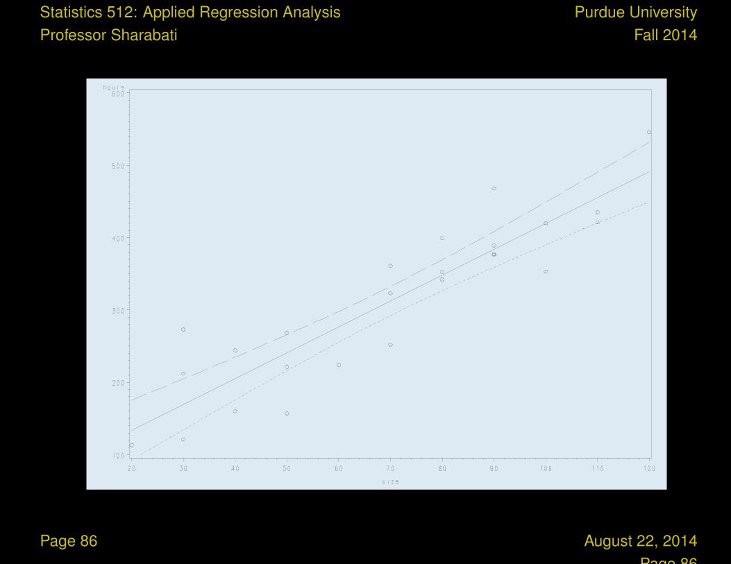
See the program knnl061x.sas for the clm (mean)and cli (individual) plots.

data a1;


input size hours;

Confidence intervals:

symbol1 v=circle i=rlclm95;

proc gplot data=a1;

plot hours*size;







Prediction Intervals:

symbol1 v=circle i=rlcli95;

proc gplot data=a1;

plot hours*size;

run;




Section 2.7: Analysis of Variance (ANOVA) Table

• Organizes results arithmetically

• Total sum of squares in Y is SSY =∑

(Yi − Y )2

• Partition this into two sources

– Model (explained by regression)

– Error (unexplained / residual)

Yi − Y = (Yi − Yi) + (Yi − Y )∑(Yi − Y )2 =

∑(Yi − Yi)

2 +∑

(Yi − Y )2

(cross terms cancel: see page 65)




Total Sum of Squares

• Consider ignoring Xh to predict E(Yh). Then the best predictor

would be the sample mean Y .

• SST is the sum of squared deviations from this predictor

SST = SSY =∑

(Yi − Y )2.

• The total degrees of freedom is dfT = n− 1.

• MST = SST/dfT

• MST is the usual estimate of the variance of Y if there are no

explanatory variables, also known as s2{Y }.

• SAS uses the term Corrected Total for this source.

“Uncorrected” is∑

Y 2i . The term “corrected” means that we

subtract off the mean Y before squaring.




Model Sum of Squares

• SSM =∑

(Yi − Y )2

• The model degrees of freedom is dfM = 1, since one

parameter (slope) is estimated.

• MSM = SSM/dfM

• KNNL uses the word regression for what SAS calls model

• So SSR (KNNL) is the same as SS Model (SAS). I prefer to

use the terms SSM and dfM because R stands for regression,

residual, and reduced (later), which I find confusing.




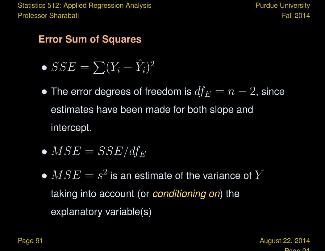
Error Sum of Squares

• SSE =∑

(Yi − Yi)2

• The error degrees of freedom is dfE = n− 2, since

estimates have been made for both slope and

intercept.

• MSE = SSE/dfE

• MSE = s2 is an estimate of the variance of Y

taking into account (or conditioning on) the

explanatory variable(s)




ANOVA Table for SLR

Source df SS MS

Model (Regression) 1∑

(Yi − Y )2 SSMdfM

Error n− 2∑

(Yi − Yi)2 SSE

dfE

Total n− 1∑

(Yi − Yi)2 SST

dfT

Note about degrees of freedom

Occasionally, you will run across a reference to “degrees of

freedom”, without specifying whether this is model, error, or total.

Sometimes is will be clear from context, and although that is sloppy

usage, you can generally assume that if it is not specified, it means

error degrees of freedom.




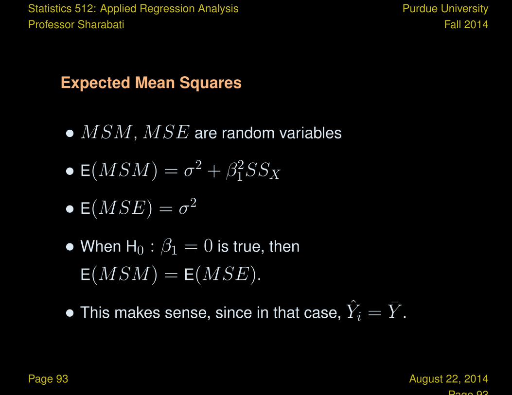
Expected Mean Squares

• MSM , MSE are random variables

• E(MSM) = σ2 + β21SSX

• E(MSE) = σ2

• When H0 : β1 = 0 is true, then

E(MSM) = E(MSE).

• This makes sense, since in that case, Yi = Y .




F -test

• F = MSM/MSE ∼ FdfM ,dfE= F1,n−2

• See KNNL, pages 69-70

• When H0 : β1 = 0 is false, MSM tends to be larger than

MSE, so we would want to reject H0 when F is large.

• Generally our decision rule is to reject the null hypothesis if

F ≥ Fc = FdfR,dfE(1− α) = F1,n−2(0.95)

• In practice, we use p-values (and reject H0 if the p-value is less

than α).

• Recall that t = b1/s(b1) tests H0 : β1 = 0. It can be shown

that t2df = F1,df . The two approaches give the same p-value;




they are really the same test.

• Aside: When H0 : β1 = 0 is false, F has a noncentral F

distribution; this can be used to calculate power.

ANOVA Table

Source df SS MS F p

Model 1 SSM MSM MSMMSE p

Error n− 2 SSE MSE

Total n− 1




See the program knnl067.sas for the program used togenerate the other output used in this lecture.

data a1;


input size hours;

proc reg data=a1;

model hours=size;

run;





Sum of Mean

Source DF Squares Square

Model 1 252378 252378

Error 23 54825 2383.71562


F Value Pr > F

105.88 <.0001




Parameter Estimates

Parameter Standard

Variable DF Estimate Error

Intercept 1 62.36586 26.17743

size 1 3.57020 0.34697

t Value Pr > |t|

2.38 0.0259

10.29 <.0001

Note that t2 = 10.292 = 105.88 = F .




Section 2.8: General Linear Test

• A different view of the same problem (testing β1 = 0). It may

seem redundant now, but the concept is extremely useful in

MLR.

• We want to compare two models:

Yi = β0 + β1Xi + εi (full model)

Yi = β0 + εi (reduced model)

Compare using the error sum of squares.




Let SSE(F ) be the SSE for the Full model, and letSSE(R) be the SSE for the Reduced Model.

F =(SSE(R)− SSE(F ))/(dfE(R) − dfE(F ))

SSE(F )/dfE(F )

Compare to the critical value

Fc = FdfE(R)−dfE(F ),dfE(F )(1− α) to test H0 : β1 = 0

vs. Ha : β1 6= 0.




Test in Simple Linear Regression

SSE(R) =∑

(Yi − Y )2 = SST

SSE(F ) = SST − SSM (the usual SSE)

dfE(R) = n− 1, dfE(F ) = n− 2,

dfE(R) − dfE(F ) = 1

F =(SST − SSE)/1

SSE/(n− 2)=

MSM

MSE(Same test as before)

This approach (“full” vs “reduced”) is more general, and

we will see it again in MLR.




Pearson Correlation

ρ is the usual correlation coefficient (estimated by r)

• It is a number between -1 and +1 that measures the strength of

the linear relationship between two variables

r =

∑(Xi − X)(Yi − Y )√∑

(Xi − X)2∑

(Yi − Y )2

• Notice that

r = b1

√∑(Xi − X)2

∑(Yi − Y )2

= b1sX

sY

Test H0 : β1 = 0 similar to H0 : ρ = 0.




R2 and r2

• R2 is the ratio of explained and total variation:

R2 = SSM/SST

• r2 is the square of the correlation between X and Y :

r2 = b21

(∑(Xi − X)2

∑(Yi − Y )2

)

=SSM

SST




In SLR, r2 = R2 are the same thing.

However, in MLR they are different (there will be a

different r for each X variable, but only one R2).

R2 is often multiplied by 100 and thereby expressed as

a percent.

In MLR, we often use the adjusted R2 which has been

adjusted to account for the number of variables in the

model (more in Chapter 6).




Sum of Mean


Model 1 252378 252378 105.88 <.0001

Error 23 54825 2383

C Total 24 307203

R-Square 0.8215

= SSM/SST = 1− SSE/SST

= 252378/307203

Adj R-sq 0.8138

= 1−MSE/MST

= 1− 2383/(307203/24)





Documents

Course Information Text: Special reprint of Applied …web.ics.purdue.edu/~wsharaba/stat512/lecture1.pdfStatistics 512: Applied Regression Analysis Professor Sharabati Purdue University