Course Guide on Introduction to Practical Geography Course

Page 1 of 133

NATIONAL OPEN UNIVERSITY OF NIGERIA

Course Guide on

Introduction to Practical Geography

Course Code: TPM105

Course Developer:

Dukiya, J. J.

Department of Urban and Regional Planning

Federal University of Technology,

Minna

Page 2 of 133

NATIONAL OPEN UNIVERSITY OF NIGERIA

National Open University of Nigeria

Headquarters

91, Cadastral Zone, Jabi Abuja

Abuja Headquarters

245 Samuel Adesujo Ademulegun Street

Central Business District

Opposite Arewa Suites

Abuja

e-mail: [email protected]

URL: www.nou.edu.ng

National Open University of Nigeria 2006

First Printed

ISBN:

All Rights Reserved

Printed by ……………..

For

National Open University of Nigeria Multimedia Technology in Teaching and Learning

Page 3 of 133

CONTENT

Introduction

Course Aim and Objectives

Course requirements and material

Study modules and Units

Assessment and Presentation Schedule

Assignment Grading

Final Examination and Grading

Course Grading System

Pathway to optimize the course benefits

Summary

Page 4 of 133

Introduction

Introduction to Practical Geography (TPM105) is a first semester course which carries

three credit units for 100 level students in the School of Management Sciences at the

National Open University, Nigeria. The coursework as an academic programme will help

to gain in-depth insight into Practical Geography.

This course guide is developed as a complement of physical geography as a prerequisite

knowledge for geospatial analysis and management. It is believed that its simplicity will

make the student comprehend faster so as to practice questions at the end of each module

and as well prepare the student for examination purposes.. It also provides some guidance

on tutor marked assignments (TMAs) for end-users.

The course is made up of four modules with 15 units spread across lecture hours and

covering areas such as basic concepts in elementary map reading, map making, including

topographical, geological and thematic maps; aerial photograph and surveying, remote

sensing and GIS, graphical and map presentation of geographical data.

Course Aim and Objectives

This course is designed to explain the concepts of global physiographic (features and

major relief patterns of the earth) in space, and associated land forms. Also the course

will teach the following: The concept of geographical data acquisition modes, Land

surveying (Lineaments, area and altitude); Aerial photograph (interpretation elements,

measurement techniques; photo scale,); Satellite imagery (platforms, sensors,

Electromagnetic Spectrums, image characteristics). Elementary map reading (locations,

types of scales. conventional signs, stereoscopic parallax, stereogram, shadow height and

area, types of maps (isoclines choropleths), relief representations and analysis, graphic

map representation,. Element of cartography; history of maps and their classification,

map symbols, earth co-ordinate system, basic form-lines and contouring, and map layout.

This course is aimed at making users familiar with the process of spatial data acquisition,

presentation and interpretation through impacted skills. It also enables them to learn how

Page 5 of 133

to evaluate physical environmental features for rational decision making at local, regional

and national levels.

This is to be achieved through the following:

i. Conceiving the basic human environmental physical features and its freezing in time

and space.

ii. Evaluating the concept of geographical data acquisition techniques and its scale

representation.

iii. Examining the various types of maps and their basic interpretation elements

iv. Understanding the basic principle of cartographic map making and areas utilization

v. Exposure to practical field data acquisition measurements and map production.

vi. Exposure to map interpretation and development of inferences for policy formation.

Course requirements and Material

To successfully complete this course, you are required to read the study units, referenced

books and other materials on the course. Each unit contains self-assessment exercises

called Student Assessment Exercises (SAE). At some points in the course, you may be

required to submit assignments for assessment purposes. At the end of the course there is

a final examination. This course runs through the whole semester and some components

of it are outlined under the course material subsection. The course definitely requires

hand-on practicals that require a computer system.

Course Material

The major component of the course and what you have to do and how you should allocate

your time to each unit in order to complete the course successfully on time are listed as

follows:

1. Course guide

2. Study unit

3. Textbook

4. Assignment

Page 6 of 133

5. Presentation schedule

Study Modules and Units

There are 15 units in this course which should be studied diligently.

i. Module 1: Overview of geographic land forms and features

Unit 1: Latitudes and longitudes and tropics

Unit 2: Geographical regions (Temperate, tropical, coastal, desert, cast)

Unit 3: Relief pattern of the earth (Drainage basin, plane land)

ii. Module 2: Geographical data acquisition techniques

Unit 1: Land surveying (Lineaments, tachymetry, area and altitude)

Unit 2: Aerial photograph (measurement techniques; photo scale,).

Unit 3: Satellite imagery (platforms, sensors, Electromagnetic Spectrums,

image Characteristics).

iii. Module 3: Elementary map and Image interpretation

Unit 1: Types of map scales.

Unit 2: Conventional signs

Unit 3: Image interpretation elements

Unit 4: Map reduction and enlargement

Unit 5: Map digitization (On-screen and Tablet)

iv. Module 4: Element of cartography

Unit 1: History of maps

Unit 2: Map classification and symbols

Unit 3 Basic form-lines, contouring and cross-sections

Unit 4: Map orientation and layouts

Page 7 of 133

Assignments and presentation Schedules

There are assignments on this course as expected of semester courses and you are

expected to do all of them by following the schedule prescribed for them in terms of

when to attempt them and possibly submit same for grading. The marks you obtain for

these assignments together with the mid-semester test will count toward the final

Continuous Assessment (CA) grade before the final examination for this course.

The assignments in this course are as follows:

Assignment 1 from Units 1 - 3 of Module 1




The schedule of presentations in this course gives the important dates for the completion

of tutor-marking assignments and attending tutorials. Note that that all assignments are to

be submitted for grading to meet the 75% required to qualify you for the final written

examination that take up to three hours. This examination will account for 70% of your

total grade

Assignments Grading (AG)

There are assignments for grading in this course that must be carried out and submitted.

You are therefore enjoined to attempt all the questions thoroughly as the AGs constitute

30% of the total score. Some of the assignment questions for the course are practical

oriented, you will therefore need a personal Laptop computer to be able to complete those

assignments apart from the information and materials contained in your text books.

However, it is required that you acquire and install the common GIS Software like

ArcGIS or Idrisi GIS to be able to view, analyse and interpret the aerial photographs or

satellite images. You should be able to also demonstrate that you have read and

researched more widely so as to have a broad and deeper understanding of the subject

matter.

Page 8 of 133

Final Examination and Grading

The final examination will be of three hours' duration and have a value of 70% of the

total course grade. The examination questions may take the pattern of the self-assessment

practice exercises and tutor-marked problems you have previously encountered. All areas

of the course will be assessed as the final examination will cover all parts of the course.

Course Grading System

The table presented below indicate the total marks (100%) allocation.

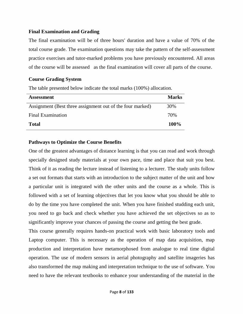
Assessment Marks

Assignment (Best three assignment out of the four marked) 30%

Final Examination 70%

Total 100%

Pathways to Optimize the Course Benefits

One of the greatest advantages of distance learning is that you can read and work through

specially designed study materials at your own pace, time and place that suit you best.

Think of it as reading the lecture instead of listening to a lecturer. The study units follow

a set out formats that starts with an introduction to the subject matter of the unit and how

a particular unit is integrated with the other units and the course as a whole. This is

followed with a set of learning objectives that let you know what you should be able to

do by the time you have completed the unit. When you have finished studding each unit,

you need to go back and check whether you have achieved the set objectives so as to

significantly improve your chances of passing the course and getting the best grade.

This course generally requires hands-on practical work with basic laboratory tools and

Laptop computer. This is necessary as the operation of map data acquisition, map

production and interpretation have metamorphosed from analogue to real time digital

operation. The use of modern sensors in aerial photography and satellite imageries has

also transformed the map making and interpretation technique to the use of software. You

need to have the relevant textbooks to enhance your understanding of the material in the

Page 9 of 133

unit and give you practical experience and skills to evaluate maps, aerial photos, and

satellite imageries, and understand the relevance of aerial information in environmental

policies formation and debates outside your studies

Suitable question and answers for self-assessments are interposed throughout the units to

help you achieve the objectives of the unit and as well prepare you for the continuous

assignments and the final examination. Should you run into any difficulty in doing all

these, please do not hesitate to ask your tutor to help you.

Summary

Introduction to Practical Geography (TPM 105) is a course that exposes the student to the

basics of practical geography such as the concepts of global physiographic (major relief

patterns of the earth) in space, season and time; and associated land forms. The concept

of geographical data acquisition modes, Land surveying (Lineaments, area and altitude);

Aerial photograph (interpretation elements, measurement techniques; photo scale,);

Satellite imagery (platforms, sensors, Electromagnetic Spectrums, image characteristics)

are also included the list of what to know are a bit long, but useful. The list includes

elementary map reading (locations, types of scales. conventional signs, stereoscopic

parallax, stereogram, shadow height and area, types of maps (isoclines choropleths),

relief representations and analysis, graphic map representation, elements of cartography;

history of maps and their classification, map symbols, earth co-ordinate system, basic

form-lines and contouring, and map layout.

If this course is completed successfully, you would have acquired the needed skills in

spatial data acquisition, evaluating and developing inferences from physical

environmental data on maps and imageries that guide environmental policy formation at

all levels. I wish you success in the course. The knowledge acquired from the course will

be useful for the other environmental related courses.

Page 10 of 133

MODULE ONE

OVERVIEW OF GEOGRAPHIC LAND FORMS AND FEATURES

Unit 1: Latitudes and longitudes and tropics

Unit 2: Measurement on Maps

Unit 3: Relief Representation (Conical hill, plateau, valley, Ridge and spur, cliff)

UNIT 1: Latitudes and Longitudes and Tropics

CONTENTS

1.0 Introduction

2.0 Objectives

3.0 Main Content

3.1 Definitions of Latitudes and longitudes and tropics

3.2 Basic Characteristics of Latitudes and longitudes and tropics

3.3 Location coordinates

3.4 Importance of Latitudes and longitudes and tropics

4.0 Conclusion

5.0 Tutor-Marked Assignment

6.0 References/Further Readings

1.0 Introduction

This unit focused on the meaning of Latitudes, longitudes and tropics, its characteristics

and usefulness in global location referencing, timing and dating. The tropic addresses the

general division of the globe according to weather and climate. This gives the bases for

grouping places nationally and internationally in reference to their location.

2.0 Objectives

At the end of this unit students should be able to:

Page 11 of 133

Define and know the meaning of Latitudes and longitudes and tropics

Understand the basic characteristics of Latitudes and longitudes and tropics

Explain the bases of grouping geographical locations according to their

revealed characteristics.

Determine the geographical coordinate of a place and tropical characteristics.

3.0 Main Content

3.1 Definition of Latitudes and longitudes and tropics

The Latitude

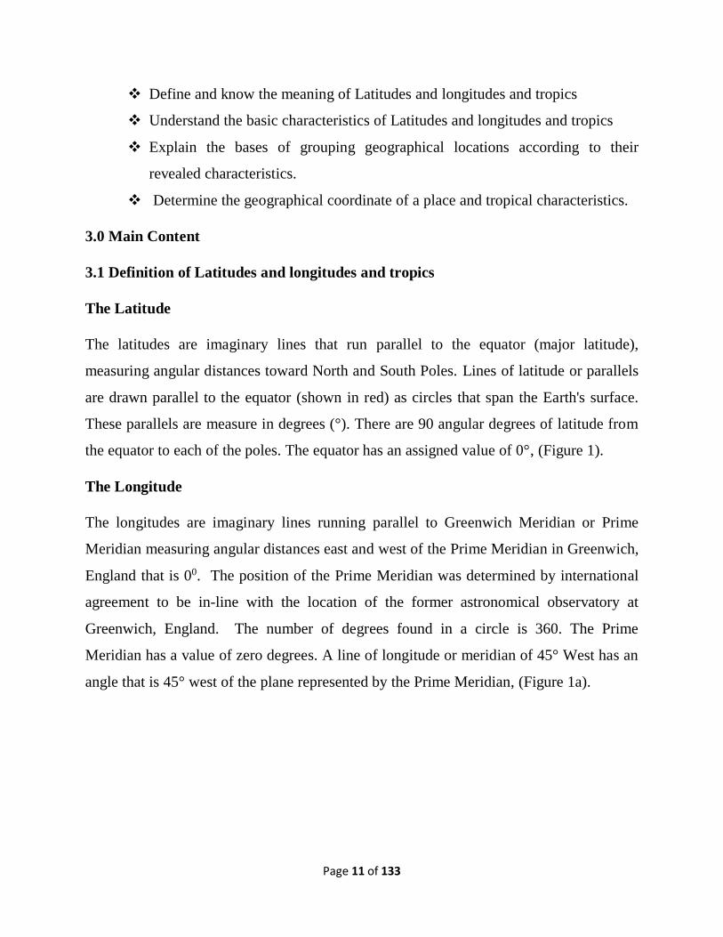
The latitudes are imaginary lines that run parallel to the equator (major latitude),

measuring angular distances toward North and South Poles. Lines of latitude or parallels

are drawn parallel to the equator (shown in red) as circles that span the Earth's surface.

These parallels are measure in degrees (°). There are 90 angular degrees of latitude from

the equator to each of the poles. The equator has an assigned value of 0°, (Figure 1).

The Longitude

The longitudes are imaginary lines running parallel to Greenwich Meridian or Prime

Meridian measuring angular distances east and west of the Prime Meridian in Greenwich,

England that is 00. The position of the Prime Meridian was determined by international

agreement to be in-line with the location of the former astronomical observatory at

Greenwich, England. The number of degrees found in a circle is 360. The Prime

Meridian has a value of zero degrees. A line of longitude or meridian of 45° West has an

angle that is 45° west of the plane represented by the Prime Meridian, (Figure 1a).

Page 12 of 133

Figure 1a, b: Measurement of latitude and longitude relative to the equator, the Prime Meridian

and the Earth's rotational or polar axis.

The Tropics and the Temperate region

The tropics are the regions within the 23½ degrees north and south of the Equator

commonly called the tropic of cancer and Capricorn respectively. They are characterised

with high temperature due the overhead sun around the equator. While the temperate

region are regions at high latitude above the tropics north and south of the Equator. They

are generally characterised with low temperature due the oblique angle of the overhead

sun to the earth sphericity.

Self Assessment exercise:

What are the parallels, the tropics, and the Prime Meridian in relation to the time zones?

3.2 Basic Characteristics of Latitudes and longitudes and tropics

The Earth is divided into degrees of longitude and latitude which help us to measure

location and time using a single standard. When used together, longitude and latitude

define a specific location through geographical coordinates. These coordinates are what

the Global Position System or GPS uses to provide an accurate locational relay.

Page 13 of 133

Longitude and latitude lines measure the distance from the Earth's Equator or central axis

- running east to west – and the Prime Meridian in Greenwich, England - running north to

south.

The Equator and the Parallels

The Equator is an imaginary line that runs around the centre of the Earth from east to

west. It is perpendicular to the Prime Meridian, the 0 degree line running from north to

south that passes through Greenwich, England. There are equal distances from the

Equator to the North Pole, and also from the Equator to the South Pole. The line

uniformly divides the northern and southern hemispheres of the planet. Because of how

the sun is situated above the Equator - it is primarily overhead - locations close to the

Equator generally have high temperatures year round. In addition, they experience close

to 12 hours of sunlight a day. Then, during the Autumn and Spring Equinoxes the sun is

exactly overhead which results in 12-hour days and 12-hour nights.

The lines of latitude run east and west, parallel to the Equator. They are used to define the

North-South position of a location on the planet. Major latitude lines include:

Equator which is 0 degrees

North Pole which is 90 degrees north

South Pole which is 90 degrees south

Arctic Circle is 66 degrees and 32' north

Antarctic Circle is 66 degrees and 32' south

Tropic of Cancer is 23 degrees and 30' north

Tropic of Capricorn is 23 degrees and 30' south

The lines of longitude run north and south. They are used to define the East-West

position of a location on the planet. They run perpendicular to the Equator and latitude

lines. Half of a longitudinal circle is called a Meridian, which is where the term comes

from in the name Greenwich Meridian or Prime Meridian. Contrary to latitude, there is

no central longitude line. However, the Prime Meridian or Greenwich Meridian is used as

Page 14 of 133

the primary reference point because it is set to 0 degrees longitude. The Prime Meridian

separates the east and west hemispheres of the Earth. Because the Earth is essentially a

spherical shape, it is considered to have 360 degrees. Therefore, the planet has been

divided into 360 longitudes as a form of measurement (see Figure 1b).


What are bases for having difference in temperature between the Tropics and the

temperate regions of the earth?

3.3 Location coordinates

By definition: the terms location and place in geography are used to identify a point or an

area on the Earth's surface. The term location generally implies a higher degree of

certainty than an entity with an ambiguous boundary, relying more on human or social

attributes of place identity and sense of place than on geometry. Place location can be

Relative, Locality, or Absolute. An example of relative is ‘Abuja is 5 km northeast of

Suleja’, locality is ‘settlement or populated place like Npape or Asokoro’, while absolute

is ‘absolute location is designated using a specific pairing of latitude and longitude in a

Cartesian coordinate grid as fully discussed below.

The geographical coordinate system measures location from only two values, despite the

fact that the locations are described for a three-dimensional surface. The two values used

to define location are both measured relative to the polar axis of the Earth. The two

measures used in the geographic coordinate system are called latitude and longitude.

Another commonly used method to describe location on the Earth is the Universal

Transverse Mercator (UTM) grid system. This rectangular coordinate system is metric,

incorporating the meter as its basic unit of measurement. UTM also uses the Transverse

Mercator projection system to model the Earth's spherical surface onto a two-dimensional

plane. The UTM system divides the world's surface into 60 - six degree longitude wide

zones that run north-south. These zones start at the International Date Line and are

Page 15 of 133

successively numbered in an eastward direction. Each zone stretches from 84° North to

80° South.

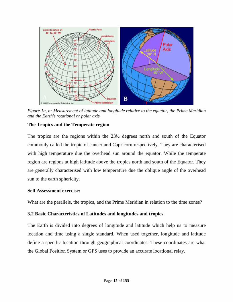
Coordinate measurements of location in the Northern Hemisphere using the UTM system

are made relative to this point in meters in eastings (longitudinal distance) and northings

(latitudinal distance). The point defined by the intersection of 50° North and 9° West

would have a UTM coordinate of Zone 29, 500000 meters east (E), 5538630 meters north

(N) (see Figures 2).

Figure 2. UTM coordinate location measurement.


Using any topographical map, determine the relative, locality and absolute location of

places of your choice.

3.4 Importance of Latitudes and longitudes and tropics

Place location and tropics are of great importance in geography and environmental

management as they help in the following areas:

i. Determination of settlement location conventionally.

ii. Description of places in relation to a well known location.

iii. Calculation of distance interval between places.

Page 16 of 133

iv. Associating locations to climatic characteristics (temperature in particular).

v. They help in spatial navigation and tracking of targets.

vi. They are used for all air and ocean navigation where there are no physical routs.

vii. Distribution of facilities spatially and determining the spread.

viii. Calculation of international-date-lines through the meridians.

ix. They help in the discussion of weather and climate and the associated characteristics


i. What are latitude and longitude, and what are the major difference between them.

ii. Discuss five (5) uses of Latitudes and longitudes and tropics.

4.0 Conclusion

We conclude that the concept of Latitudes and longitudes and tropics is vital for all

countries of the world because of its importance in locating and describing places

conventionally while relating them to all natural and artificial attributes of the world.


i. With suitable examples, give a detailed discussion of five (5) uses of Latitudes and

longitudes and tropics.

ii. What are the major differences between the parallels and the great meridian

iii. With the topographical map given, determine the relative and absolute location of

Zuba in relation to Dutse Alhaji.


George, M., and Cole, PE PLS (2005). Fundamentals of Surveying: Sample Examination,

Professional Publications, Inc.; Second edition. ISBN-13: 978-1591260455

Raymond, E.P., and Walter, W. (2015). Basic Surveying, 4th Edition. Routledge. ISBN-

10: 1138168742

Page 17 of 133

UNIT 2: MEASUREMENT ON MAPS

CONTENTS

1.0 Introduction

2.0 Objectives

3.0 Main Content

3.1 Distance measurement

3.2 Directional measurement on maps

3.3 Area measurement on maps

3.4 Use of Geographical Positioning System (GPS) for position and distances

4.0 Conclusion



1.0 Introduction

In unit 1, we have been exposed to the world as a globe and place location that can be

conventionally identified or described on maps. There is therefore the need to carry out

some measurement to determine distances, area coverage and relative angular bearing to

one another. Although it is possible to create maps that are somewhat equidistant, yet

these types of maps have some form of distance distortion that require some form of

manipulation through scale usage. Equidistance maps can only control distortion along

either lines of latitude or lines of longitude. Distance is often correct on equidistance

maps only in the direction of latitude.

Like distances, relative direction is difficult to measure on maps because of the distortion

produced by projection systems. However, this distortion is quite small on large scale

maps. Direction is usually measured with reference to the location of North or South

Pole. Directions determined from these locations are said to be relative to True North or

True South.

Page 18 of 133

2.0 Objectives

At the end of this unit you should be able to:

Carry out distance measurements between two or more locations on the map

with reference to the map scale manually or digitally.

Determine location reference bearing of places on the map with reference to

the hemispheric location

Carry out area measurement on maps manually or digitally.

Determine Density of features distribution and degree of dispersion

Get acquitted with the use of GPS devices for simple place location and

distance measurement.

3.0 Main Content

3.1 Distance measurement

Distance measurement on a straight course is quite simple compared to measurement of

irregular features like river course or road. Measuring distances as the scroll flies are

carried out by the use of a ruler or straight edge in between the two locations, and then

convert the measured distance into a real world distance using the map's scale.

For example, if we measured a distance of 10 cm on a map that had a scale of 1:10,000,

we would multiply 10 (distance) by 10,000 (scale). Thus, the actual distance in the real

world would be 100,000 cm which is equivalent to 1km distance interval.

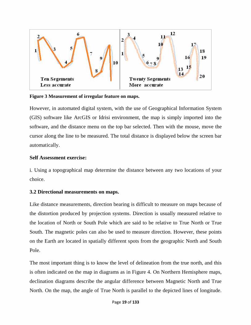
For measurement along irregular feature, one can use a string or straight edge that is

orientated along the feature’s configuration as demonstrated in figure 3 and then convert

the measured distance into a real world distance using the map's scale as in straight

course above. Another method for measuring curvilinear map distances is to use a

mechanical device called an opisometer. This device uses a small rotating wheel that

records the distance travelled. The recorded distance is measured by this device either in

centimeters or inches.

Page 19 of 133

Figure 3 Measurement of irregular feature on maps.

However, in automated digital system, with the use of Geographical Information System

(GIS) software like ArcGIS or Idrisi environment, the map is simply imported into the

software, and the distance menu on the top bar selected. Then with the mouse, move the

cursor along the line to be measured. The total distance is displayed below the screen bar

automatically.


i. Using a topographical map determine the distance between any two locations of your

choice.

3.2 Directional measurements on maps.

Like distance measurements, direction bearing is difficult to measure on maps because of

the distortion produced by projection systems. Direction is usually measured relative to

the location of North or South Pole which are said to be relative to True North or True

South. The magnetic poles can also be used to measure direction. However, these points

on the Earth are located in spatially different spots from the geographic North and South

Pole.

The most important thing is to know the level of delineation from the true north, and this

is often indicated on the map in diagrams as in Figure 4. On Northern Hemisphere maps,

declination diagrams describe the angular difference between Magnetic North and True

North. On the map, the angle of True North is parallel to the depicted lines of longitude.

Page 20 of 133

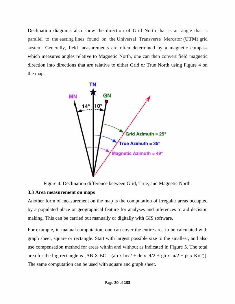
Declination diagrams also show the direction of Grid North that is an angle that is

parallel to the easting lines found on the Universal Transverse Mercator (UTM) grid

system. Generally, field measurements are often determined by a magnetic compass

which measures angles relative to Magnetic North, one can then convert field magnetic

direction into directions that are relative to either Grid or True North using Figure 4 on

the map.

Figure 4. Declination difference between Grid, True, and Magnetic North.

3.3 Area measurement on maps

Another form of measurement on the map is the computation of irregular areas occupied

by a populated place or geographical feature for analyses and inferences to aid decision

making. This can be carried out manually or digitally with GIS software.

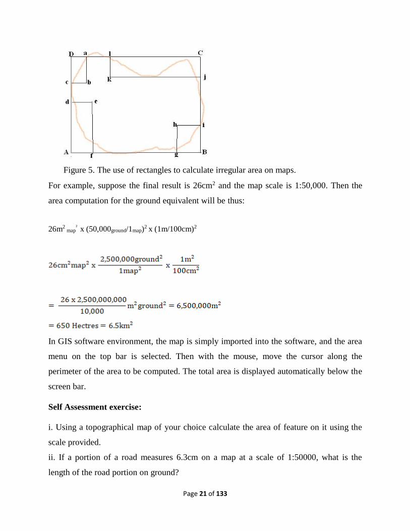
For example, in manual computation, one can cover the entire area to be calculated with

graph sheet, square or rectangle. Start with largest possible size to the smallest, and also

use compensation method for areas within and without as indicated in Figure 5. The total

area for the big rectangle is [AB X BC – (ab x bc/2 + de x ef/2 + gh x hi/2 + jk x Ki/2)].

The same computation can be used with square and graph sheet.

Page 21 of 133

Figure 5. The use of rectangles to calculate irregular area on maps.

For example, suppose the final result is 26cm2 and the map scale is 1:50,000. Then the

area computation for the ground equivalent will be thus:

26m2 map

² x (50,000ground/1map)2 x (1m/100cm)2

In GIS software environment, the map is simply imported into the software, and the area

menu on the top bar is selected. Then with the mouse, move the cursor along the

perimeter of the area to be computed. The total area is displayed automatically below the

screen bar.


i. Using a topographical map of your choice calculate the area of feature on it using the

scale provided.

ii. If a portion of a road measures 6.3cm on a map at a scale of 1:50000, what is the

length of the road portion on ground?

Page 22 of 133

3.4 Determine Density of features distribution and degree of dispersion

Density measure levels of compactness or concreteness of features distribution over a

geographical space, which is the number or population per square kilometre. For

instance, the density distribution of schools, health centres or public water points may be

assessed for planning purposes. It is calculated by the formula: D= P/A

Where:

D = Density

P = Population

A = Area

The population (P) is the enumeration or counting of the total features of interest on the

map, while the total space area is determined as earlier discussed above using the scale of

the map under consideration in square kilometre (km2)). Then apply the formula above to

determine the density of the features’ distribution.

To determine the degree level of random or uniform clustering, or dispersion of map

features, the Quadrat Analysis (QA) technique or the Nearest Neighbour Analysis (NNA)

technique can be applied. Using the NNA for instance, one can measure the degree of

clustering of private health centres with the following steps:

i. On a straight line, measure the distance between a centre and its nearest neighbour

on the map. Note that in some cases two centres within an area may be located

closer to one another than they are to any other centre. In that case the same distance

is measured twice.

ii. The distance measurements on map in centimetres (metric system); must be

converted to kilometres (or metres) using the map scale, to find the ground

equivalent of each measurement. For instance, if the distance from centre A to its

nearest neighbour centre E is 2cm, and given that the map scale is 1:50,000, the

distance in kilometres between health centre A and E will be:

Page 23 of 133

= 1km

iii. Find the total area of the place within which the centres are located using the earlier

area computation method and convert to square kilometres using the map scale. If

the place is rectangular in shape, the formula for finding the area of a rectangle is

used. But if the area has an irregular shape, then any of the methods for calculating

the area of an irregular shape can be used.

i. Having measured the distances between the centres and the area, then the Nearest

Neighbour index is calculated thus:

R = rA/rE

Where

R = Near neighbour index (NB: this index ranges in value from 0 (aggregation)

through 1 (random) to 2.15 (uniform)).

rA = observed mean distance.

rE = expected mean distance in a random distribution. rE = ½(p(-½)), where

p = the observed density of centres in the place under consideration (i.e. density is

number of points divided by area)

3.5 Use of Geographical Positioning System (GPS) for position and distances

Determination of feature location in the field and on map manually was hitherto

problematic, but technology has simplify this with the use of electronic device like the

GPS that measure to the nearest 5m – 10m accuracy depending on the model capacity.

Handheld Global Positioning Systems (GPS) receivers can determine latitude, longitude,

and elevation anywhere on or above the Earth's surface from signals transmitted by a

number of satellites. These units can also be used to determine direction; distance

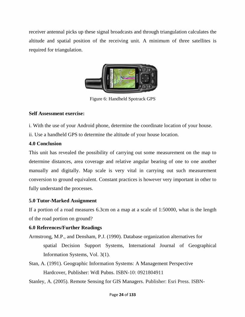
travelled, and determines routes of travel in field situations. Garmine 78 or Spotrack are

common handheld GPS available commercially, (see Figure 6). The device receiver

antennal receives the radio signal transmissions from several satellites that are

broadcasted continually to determine the coordinate location of the point of use. The

Page 24 of 133

receiver antennal picks up these signal broadcasts and through triangulation calculates the

altitude and spatial position of the receiving unit. A minimum of three satellites is

required for triangulation.

Figure 6: Handheld Spotrack GPS


i. With the use of your Android phone, determine the coordinate location of your house.

ii. Use a handheld GPS to determine the altitude of your house location.

4.0 Conclusion

This unit has revealed the possibility of carrying out some measurement on the map to

determine distances, area coverage and relative angular bearing of one to one another

manually and digitally. Map scale is very vital in carrying out such measurement

conversion to ground equivalent. Constant practices is however very important in other to

fully understand the processes.


If a portion of a road measures 6.3cm on a map at a scale of 1:50000, what is the length

of the road portion on ground?


Armstrong, M.P., and Densham, P.J. (1990). Database organization alternatives for

spatial Decision Support Systems, International Journal of Geographical

Information Systems, Vol. 3(1).

Stan, A. (1991). Geographic Information Systems: A Management Perspective

Hardcover, Publisher: Wdl Pubns. ISBN-10: 0921804911

Stanley, A. (2005). Remote Sensing for GIS Managers. Publisher: Esri Press. ISBN-

Page 25 of 133

13: 978-1589480810

Aronoff, S. (1989). Geographic Information Systems: A Management Perspective. WDL

Publications, Ottawa.

Page 26 of 133

UNIT 3: RELIEF REPRESENTATION (CONICAL HILL, PLATEAU, VALLEY,

RIDGE AND SPUR, CLIFF)

CONTENT

1.0 Introduction

2.0 Objectives

3.0 Main Content

3.1 General descriptions of relief maps

3.2 Analysis of major terrain configuration

3.3 General Slope Analysis

3.4 Gradient computation and analysis

4.0 Conclusion



1.0 Introduction

Relief in geography is the surface configuration of the earth at a point in time, the

difference in elevation between the high and low points, usually measured as relative

relief. The earth’s surface is not uniform and it varies from mountains to hills to plateaus

and plains. The general configuration of the earth’s surface in the form of elevation and

depressions are known as relief features of the earth and the map showing these features

is called a relief map. These relief features of a land surface are shown on a map by

means of various techniques such as contour lines, hachure, hill shading, spot heights,

bench marks and trigonometric stations.

2.0 Objectives

At the end of this unit users of this material should be able to:

Be able to identify major map relief features

Classify and interpret different slopes as presented by contour lines

Analyse and develop inferences from terrain configuration

Page 27 of 133

Calculate vertical and horizontal interval for gradient analysis

3.0 Main Content

3.1 General descriptions of relief maps

Relief maps generally gives information on terrain features like mountains, valleys,

slopes, depression as defined by contours or other representations (hachuring or

shadowing). The shape of any terrain influences flow of surface water, transport of

sediment, climate both on local and regional scales, nature and distribution of habitats for

plant and animal species, and migration patterns of many animal species. It is also an

expression of geological and weathering processes that have contributed to its formation.

Knowledge of terrain morphology also is essential for any engineering or land-

management endeavours that affect or disturb the surface of the land.

Earth’s surface is a dynamic interface across which the atmosphere, water, biota, and

tectonics interact to transform rock into landscapes with distinctive features crucial to the

function and existence of water resources, natural hazards, climate, biogeochemical

cycles, and life. Landforms are defined as specific geomorphic features on the surface of

the Earth, ranging from large-scale features such as plains and mountain ranges to minor

features such as individual hills and valleys. The ability to map landforms is an important

aspect of any environmental or resource analysis and modelling effort. Traditionally,

mapping of the aspects of the environment has been accomplished through in situ surveys

Another way of representing relief on maps is hill hachuring which is short lines with

different tone drawn slope-wise to show the shape of the land. This can also be done

through contour layering in which, for example, if the height of an area ranges from 0 to

500m, the land can be divided into any convenient height zones such as 0 – 100m, 100 –

200m, 200 – 300m, 300 – 400m, 400 – 500m. Then different colour shades are used to

represent each height zone or contour layer. Conventionally, blue is used to represent

water bodies, green for lowlands, yellow for middle grounds, brown for highlands and

white for snow capped hill or mountain tops.

Page 28 of 133

Also, Trigonometric Stations, Spot heights, and Bench Marks can be used to represent

relative heights on the relief maps. On a map a spot height is indicated with a dot and the

actual height value written beside the dot, while Bench Mark (BM) is a permanent land

survey mark inscribed on an object such as wall, building, roadside, or bridge to indicate

the exact height above sea level of that spot.

3.2 Analysis of major terrain configuration

In carrying out terrain analysis, apart from the shape and closeness of the contour lines,

the relative location in term of hemisphere or tropics is of major importance. A full

knowledge of the map geographical location will help in associating the feature

accurately classify or describe the shape.

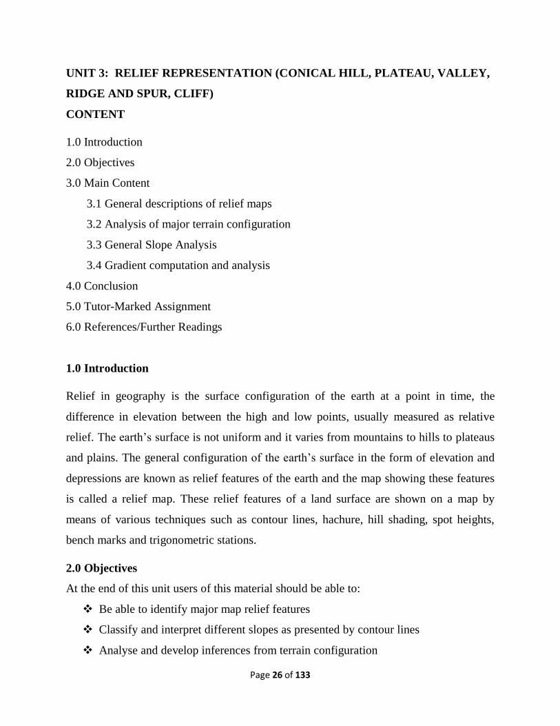
Slopes are generally classified into gentle, steep, concave, convex and irregular or

undulating. The contours of different types of slopes show a distinct spacing pattern.

When the contours representing a slope are far apart and the degree or angle of slope of

the feature is very low, the slope will be said to be gentle. But when the degree or angle

of slope of a feature is high and the contours are closely spaced, they are steep slope as

Figure 7.

Figure 7: Steep slope as a pure and flat base.

Page 29 of 133

3.3 General Slope Analysis

Slope according to Savindra S. and Srivastava R. (1974), is an angular inclination of

region between crests and base of the valley. Slope occurrences may as a result of:

Geological structure, climate, vegetation cover, drainage network, drainage texture and

frequency, bifurcation ration, absolute relief, relative relief, and erosion. It is important

geomorphic attributes in the study of landforms of a drainage basin”. Slope is therefore

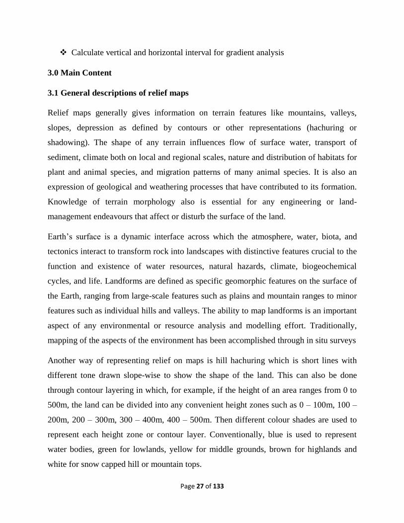
upward or downward inclination of ground between mountain and valley. The shape of

the slope may be concave, convex, free face and rectilinear which are known as

morphology of slope. The convex element originates in the crest; free face element is

found in steep inclination of slope and is shown like a cliff. The concave element is

defined by the basal section of an ideal mountain slope, (figure 8).

Fig.ure 8 Show the element of slope

Slope is a key factor in describing and analysing landforms and the development and

formation of landforms are dependent on the shape of slope and process of slope

development. So, the analysis of slope is very important in morph metric analysis. The

main purpose of the present slope analysis is to study the characteristics and

distributional pattern of average slope. There are various techniques of slope analysis

which include that of Finsterwalder S. (1890), which is to determine the total length of

contour in the entire area and then apply the formula used to calculate the average slope

of the study area:-

Page 30 of 133

It has been established that the erodibility of a watershed can be compared with its

average slope and that the more the percentage of slopes; the more will be the erosion all

thing been equal. The analysis of an area can be divided into four major slope groups via:

1. Gentle slope (< 100)

2. Moderate slope (100-200)

3. Steep slope (200 -300)

4. Very steep slope (> 300)

Slope Aspect which is a very significant component in slope analysis defines the

direction of compass that a slope surface faces. Aspect depicts clock-wise direction from

the north which also shows directional measures of slope. The major classifications of

aspect are as follows;

North

North –East

East

South- East

South

South – West

West and

North – West

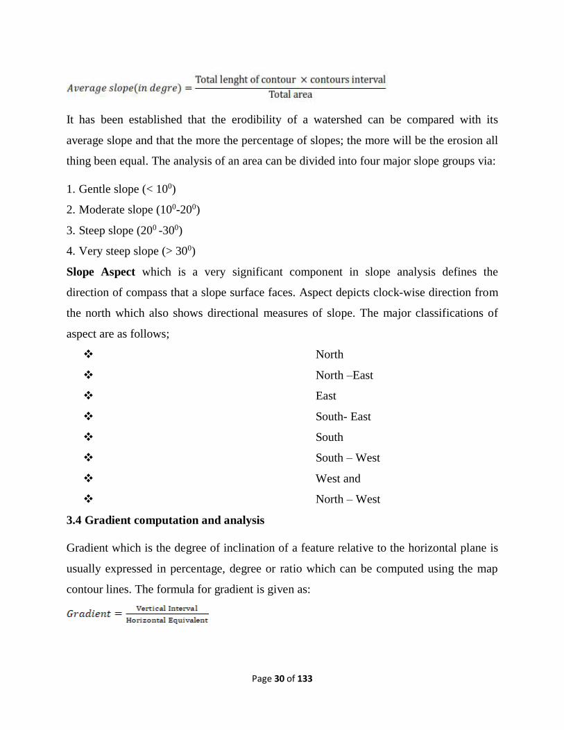
3.4 Gradient computation and analysis

Gradient which is the degree of inclination of a feature relative to the horizontal plane is

usually expressed in percentage, degree or ratio which can be computed using the map

contour lines. The formula for gradient is given as:

Page 31 of 133

Figure 9: Typical terrain with gentle slope contouring.

Given a topographical map as in figure 9, the following steps will be followed to

calculate the gradient between point A and B:

i. Knowing that contour lines are line joining places of equal height on the map,

subtract the height value for B from that of A vertical interval is (900 – 300) =

600m.

ii. Determine the horizontal distance between A and B with a straight edge and apply

the map scale to the value obtained. For instance, if the distance from centre A to

B is 20cm, and given that the map scale is 1:50,000, the distance in kilometres

between them will be:

= 10km

G m

iii. By interpretation, here for every one meter horizontal travel, there is a 0.06 meter

of altitude gained. This is a flat terrain as indicated by the contour in figure 9.

iv. Note that here is assumed that the Topo Sheet is in metric (inches and feet) as

against imperial (centimetres and meter).

Page 32 of 133

4.0 Conclusion

Surface relief in any given locality is a major factor determining the configuration of the

area and the use to which such area can be put. There is always the need to have proper

analysis of a given terrain to aid decision makers on land uses and facility distribution;

you will do yourself a great favour by carrying series of self assessment on this topic to

be to understand environmental issues.


i. Using the given topographical map, calculate the gradient between BM 65 and BM 80.

ii. To what extent do slope analysis influence transport rout sitting.


Campbell, J. (1984). Introductory Cartography. 2nd Edition, Publisher: William C Brown

Pub; 2nd edition Prentice Hall, New Jersey. ISBN-13: 978-0697108265

Dobson, J.E. (1983). Automated Geography, Professional Geographer 35:135–43.

https://doi.org/10.1111/j.0033-0124.1983.00135.x

Yuji, M. (NA). Fundamentals of Surveying Theory and Samples Exercises. Division of

Spatial Information Science Graduate School Life and Environment Sciences,

University of Tsukub

http://giswin.geo.tsukuba.ac.jp/sis/tutorial/fundamentals_of_surveying.pdf

https://doi.org/10.1111/j.0033-0124.1983.00135.x

Page 33 of 133

MODULE TWO

GEOGRAPHICAL DATA ACQUISITION TECHNIQUES

Unit 1: Land surveying (Lineaments, tachymetry, area and altitude)

Unit 2: Aerial photograph (measurement techniques; photo scale,).

Unit 3: Satellite imagery (platforms, sensors, Electromagnetic Spectrums, Characteristic

image)

UNIT 1: LAND SURVEYING (LINEAMENTS, TACHYMETRY, AREA AND

ALTITUDE)

CONTENT

1.0 Introduction

2.0 Objectives

3.0 Main Content

3.1 Types of surveying and their roles

3.2 Convectional map symbols

3.3 Distance and types of angular measurements

3.4 The use of field books in detail survey

3.5 Basic survey traverse

3.6 Basic levelling activities

4.0 Conclusion



1.0 Introduction

Surveying according to Michael Minchin (2016), is the process of determining the

relative position of natural and manmade features on or under the earth’s surface, the

presentation of the information so determined either graphically in the form of plans or

Page 34 of 133

numerically in the form of tables, and the setting out of measurements on the earth’s

surface. It usually involves measurement, calculations, the production of plans, and the

determination of specific locations. Surveyors may be involved in determining heights

and distances; setting out buildings, bridges and roadways; determine areas and volumes

and to draw plans at a predetermined scale.

Apart from areas of specialties in (Topographic, Engineering, Cadastral, hydrographic,

Aerial, Astronomic, Mining, and Computing), surveying can generally be grouped into

Plane Surveying or Geodetic surveying which will be discuss later.

While survey processes include: Reconnaissance, Measurement and Marking, Plan

Preparation, surveyors must have a thorough knowledge of mathematics, particularly

geometry and trigonometry and calculus, they must also have a thorough knowledge of

methods in all the allied courses like: geodesy, photogrammetry, remote sensing,

cartography and computers, with some competence in economics (including office

management), geography, geology, astronomy and town planning.

2.0 Objectives

At the end of this unit users of this material should be able to:

Understand how map data are acquired through manual and electronic devices

Be able to understand types of surveying and their role in the built environment.

Have basic knowledge of Aerial photograph and interpretation elements

Understand Satellite imagery platforms and characteristics

3.0 Main Content

3.1 Types of surveying and their roles

Plane Surveying focuses on the earth surface with the assumption that the earth’s surface

is plane and therefore ignore the curvature nature of the earth.

While the Geodetic surveying is concerned with determining the size and shape of the

earth and also provides a high-accuracy standard framework that are necessary for the

Page 35 of 133

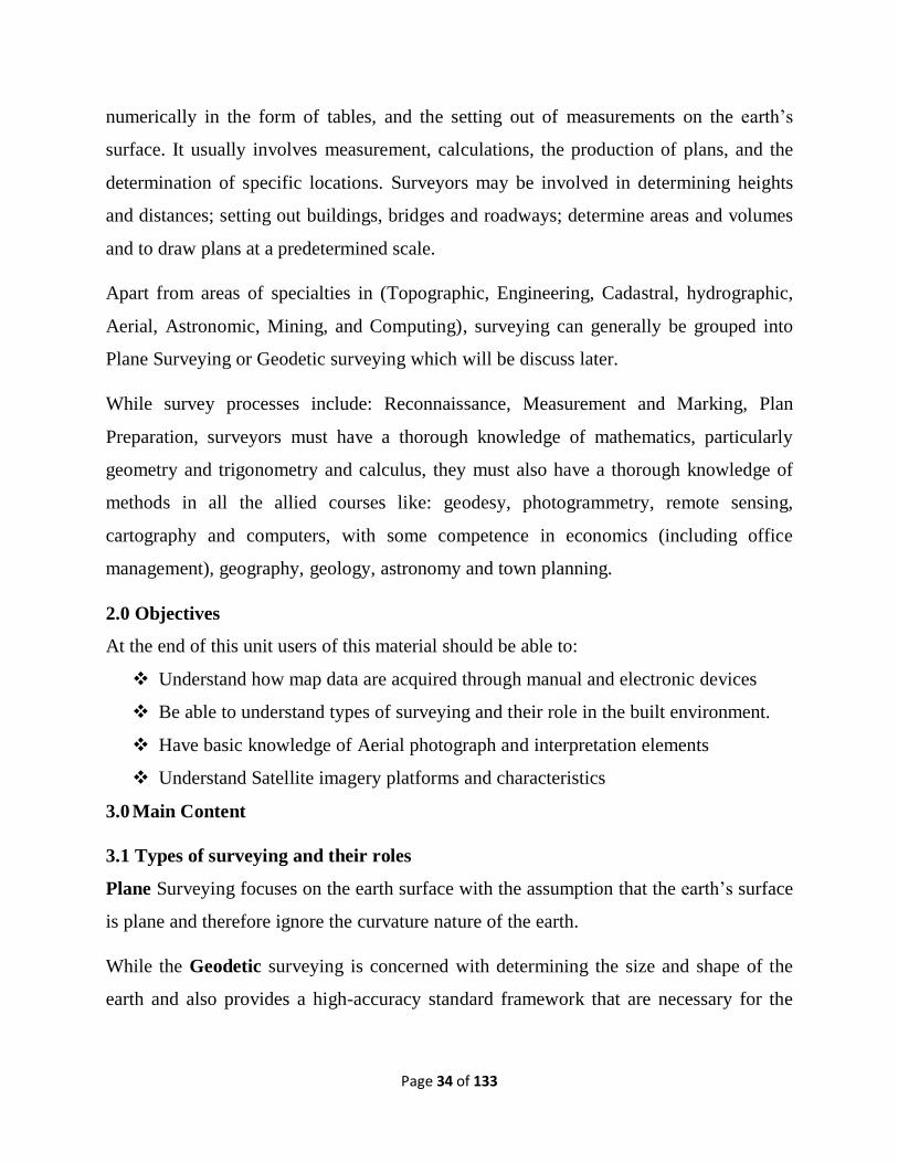
control of lower order surveys. It cover relatively large areas (e.g. a state or country) for

which the effects of earth curvature must be considered, see figure 10.

Figure 10: Geodetic and Plane surveying.

Role of a Surveyor

The surveyor has a responsibility to the community in general, to ensure that work

undertaken by his team does not damage property or interfere with members of the

community. Permission must be sought before accessing private property or before

removing trees or shrubbery to enable survey measurements. The tasks performed by a

surveyor will depend on which branch of surveying they practise in. The most common

tasks involve the determination of height and distances.

i. Cadastral Surveyors are concerned with determination of property boundaries.

ii. Topographical Surveyors are involved in the location of detail on the earth’s surface

for the production of maps.

iii. Engineer Surveyor’s tasks include the setting out of buildings, sewers, drains, bridges

and roadways; determining areas and volumes of regular and irregular figures; the

preparation of detailed drawings and plans.

iv. While Mine Surveyor’s main tasks include the setting out of mine lease boundaries

and the calculation of end-of-month volumes.

3.2 Concept of map symbols

Maps are usually drawn using graphic or simply symbolising the various geographical

phenomena shown on the map. When we engage in map reading and analysis we are only

Page 36 of 133

trying to decode the symbols in order to understand their meanings and, hence, the

information they bear and convey. Understanding map symbols and their meanings helps

us to properly interpret maps and derive the information being communicated through the

maps. The symbols are used to code or set data and present it in form of a diagram or

illustration which is part of the sign language of the map presented in the map’s legend or

key.

There are different types of symbols that can be used to produce a map which can

conveniently be grouped into three broad categories namely point symbols, line symbols

and area symbols. Note that this grouping is also in line with our grouping of

geographical features into point features, line features and area features. There are also

others like conventional symbols, pictorial symbols, and literal or textual symbols.

i. Point Symbols

On the map point symbols are shown as individual discrete dots existing at single spots or

locations. The dots, however, are not always circular. In other words, point symbols

could be of various shapes and sizes too, Moreso, a point symbol can be used to represent

a qualitative value or a quantitative value. As a qualitative symbol, a point symbol simply

shows where individual features are located; like petrol station, trigonometric station,

spot height or benchmark. On the other hand, if used as a quantitative symbol it indicates

the quantity or amount of the feature it represents. For instance, one dot can be used to

represent 5000 people in a dot map showing the distribution of human population in a

region(s).

ii. Line Symbols

Line symbols are used to represent one-dimensional or linear features such as roads,

rivers, railways, pipelines, and power or telecommunication cables. Like point symbols,

some line symbols are used to show qualitative values, while some (e.g. contour lines)

are used to show quantitative values. Line symbols (e.g. flow maps) can also be used to

Page 37 of 133

show the degree of flow of people, goods, energy, animals etc. from one location to

another.

iii. Area Symbols

Area symbols are used to map two-dimensional or polygonal features that significantly

cover a wide area of land. Examples of areal features include lakes, lagoons, farmlands,

school compounds, state, country, and so on. There are qualitative area symbols as well

as quantitative area symbols. The area symbol can also be in form of a colour or pattern.

iv. Literal or Textual Symbols

These are symbols that are derived from the abbreviation of some words; hence they are

in form of texts or letters. They are used to indicate the locations of the features they

represent as listed below:

Sch = School

Mkt = Market

Ch = Church

RH = Rest House

PO = Post Office

Hosp = Hospital

3.3 Distance and types of angular measurements

In surveying, the basic measurement is that of distance and this can be measured by many

methods, including:

a. pacing

b. odometer readings

c. optical range finders

d. tacheometry

e. subtense bar

f. taping or chaining

g. electronic distance measurement.

Page 38 of 133

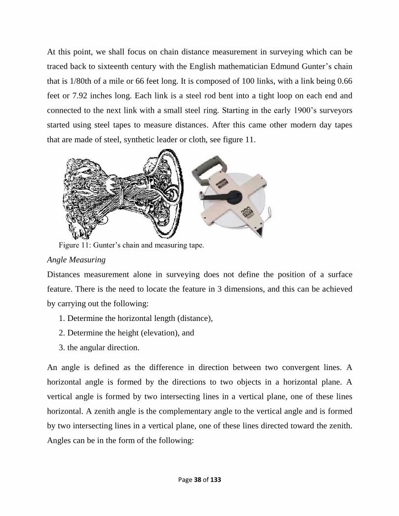
At this point, we shall focus on chain distance measurement in surveying which can be

traced back to sixteenth century with the English mathematician Edmund Gunter’s chain

that is 1/80th of a mile or 66 feet long. It is composed of 100 links, with a link being 0.66

feet or 7.92 inches long. Each link is a steel rod bent into a tight loop on each end and

connected to the next link with a small steel ring. Starting in the early 1900’s surveyors

started using steel tapes to measure distances. After this came other modern day tapes

that are made of steel, synthetic leader or cloth, see figure 11.

Figure 11: Gunter’s chain and measuring tape.

Angle Measuring

Distances measurement alone in surveying does not define the position of a surface

feature. There is the need to locate the feature in 3 dimensions, and this can be achieved

by carrying out the following:

1. Determine the horizontal length (distance),

2. Determine the height (elevation), and

3. the angular direction.

An angle is defined as the difference in direction between two convergent lines. A

horizontal angle is formed by the directions to two objects in a horizontal plane. A

vertical angle is formed by two intersecting lines in a vertical plane, one of these lines

horizontal. A zenith angle is the complementary angle to the vertical angle and is formed

by two intersecting lines in a vertical plane, one of these lines directed toward the zenith.

Angles can be in the form of the following:

Page 39 of 133

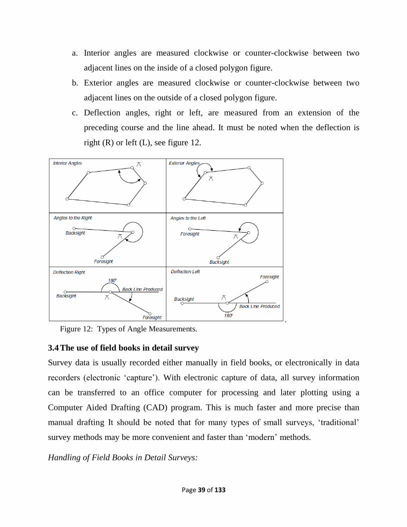
a. Interior angles are measured clockwise or counter-clockwise between two

adjacent lines on the inside of a closed polygon figure.

b. Exterior angles are measured clockwise or counter-clockwise between two

adjacent lines on the outside of a closed polygon figure.

c. Deflection angles, right or left, are measured from an extension of the

preceding course and the line ahead. It must be noted when the deflection is

right (R) or left (L), see figure 12.

.

Figure 12: Types of Angle Measurements.

3.4 The use of field books in detail survey

Survey data is usually recorded either manually in field books, or electronically in data

recorders (electronic ‘capture’). With electronic capture of data, all survey information

can be transferred to an office computer for processing and later plotting using a

Computer Aided Drafting (CAD) program. This is much faster and more precise than

manual drafting It should be noted that for many types of small surveys, ‘traditional’

survey methods may be more convenient and faster than ‘modern’ methods.

Handling of Field Books in Detail Surveys:

Page 40 of 133

• Draw neat sketches of the features on the lot under survey, to show true shapes, as

far as

possible.

• Maintain true relationships between positions of features, as far as possible.

•Each point radiated should have a point number shown both on the sketch and in the

tabulations - this allows easy crosschecking when plotting, especially if an error has

occurred.

• For each radiated point show: Point No., Description, Horizontal Angle, Vertical

Angle

Distance

For typical suburban detail surveys, field notes should show:

i. buildings − construction, types and use,

ii. adjoining land use,

iii. boundary (fence) distances,

iv. measurements along all sides of buildings,

v. distances between buildings,

vi. distances between fences and buildings,

vii. fencing type and height,

viii. lengths and widths of paths and driveways,

ix. distances from front boundary corners to road centre-lines,

x. positions of sumps − storm-water and sewerage,

xi. approximate height and diameter of trees,

xii. overhead obstructions − power and telephone lines, overhanging trees

etc.

3.5 Basic survey traverse

A traverse is a multiple of related points or stations which, when connected together with

angular and linear values, form a framework. It is a successive straight line along or

through the area to be surveyed. The directions and lengths of these lines are determined

Page 41 of 133

by measurements taken in the field. This operation is currently the most common of

several possible methods for establishing a series or network of monuments with known

positions on the ground. Such monuments are referred to as horizontal control points and

collectively, they comprise the horizontal control for the project. There are several types

or designs of traverses that can be utilized on any given survey. The terms open and

closed are used to describe certain characteristics of a traverse. If not specified, they are

assumed to refer to the mathematical rather than geometrical properties of the traverse.

If a traverse proceeds from one coordinated (fixed) point to another, it is known as a

closed traverse. Note that a closed traverse may either close back to its starting point or

to any other coordinated point. It is, therefore, able to be checked and adjusted to fit

accurately between these known points.

An open traverse does not close on to a known point. The end of the traverse, point F, is

left ‘swinging’ with no accurate means of checking angular or linear errors that may have

occurred between A and F. The only check would be to repeat the whole traverse, or

resurvey in the opposite direction.

Figure 13: Examples of survey traverses.

Traversing may be employed in the following:

a. Control - establishing a system of horizontal control for setting out and surveying

detail of engineering or mining projects

b. Setting out - the position of design features such as roads, buildings, sewerage and

drainage lines

c. Surveying detail - pick-up of natural and artificial features in relation to control

Page 42 of 133

d. Cadastral - establishment of original boundaries and subdivision into parcels of

land

e. Geodetic - traversing to provide major control for mapping large areas.

3.6 Basic levelling activities

Levelling is the process of determining the difference in elevation between two or more

points on the earth's surface mostly for engineering works, both in the design stages and

during construction operations. There are many different ways of obtaining differences in

height, but we are focusing on spirit levelling in depth with brief outline of electronic

levelling. The other most common approaches are outlined below:

i. Barometric Heighting

Barometric Heighting is the determination of differences in height based on the premise

that atmospheric pressure decreases as altitude increases. The difference in atmospheric

pressure is obtained by using an aneroid barometer. This method is suitable for

exploratory surveys where portability, compactness and time are important

considerations, and a high degree of accuracy is not required.

ii. Trigonometrical Heighting

Trigonometrical heighting is the determination of difference in height by measuring

vertical angles and distances. The term often relates to long sights where allowance must

be made for the curvature of the earth. To obtain an accurate difference in height between

the two points, it is essential that both the distance and the vertical angle is measured

from both the observation station to the target station and from the target station to the

observation station.

iii. Electronic Levelling

This is a general term used to describe not so much the method, but the type of equipment

used. It includes alignment lasers, rotating head lasers and digital read-out levels.

Page 43 of 133

The Level

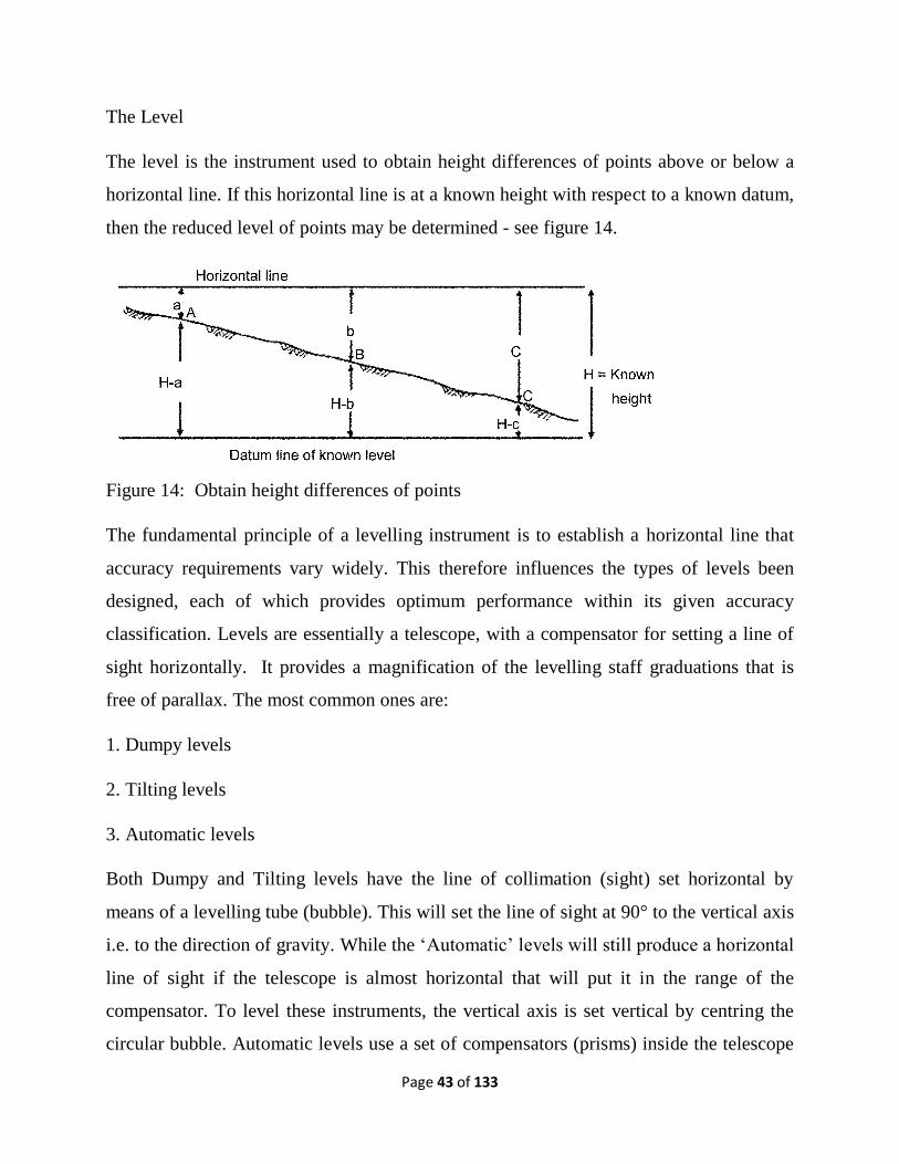
The level is the instrument used to obtain height differences of points above or below a

horizontal line. If this horizontal line is at a known height with respect to a known datum,

then the reduced level of points may be determined - see figure 14.

Figure 14: Obtain height differences of points

The fundamental principle of a levelling instrument is to establish a horizontal line that

accuracy requirements vary widely. This therefore influences the types of levels been

designed, each of which provides optimum performance within its given accuracy

classification. Levels are essentially a telescope, with a compensator for setting a line of

sight horizontally. It provides a magnification of the levelling staff graduations that is

free of parallax. The most common ones are:

1. Dumpy levels

2. Tilting levels

3. Automatic levels

Both Dumpy and Tilting levels have the line of collimation (sight) set horizontal by

means of a levelling tube (bubble). This will set the line of sight at 90° to the vertical axis

i.e. to the direction of gravity. While the ‘Automatic’ levels will still produce a horizontal

line of sight if the telescope is almost horizontal that will put it in the range of the

compensator. To level these instruments, the vertical axis is set vertical by centring the

circular bubble. Automatic levels use a set of compensators (prisms) inside the telescope

Page 44 of 133

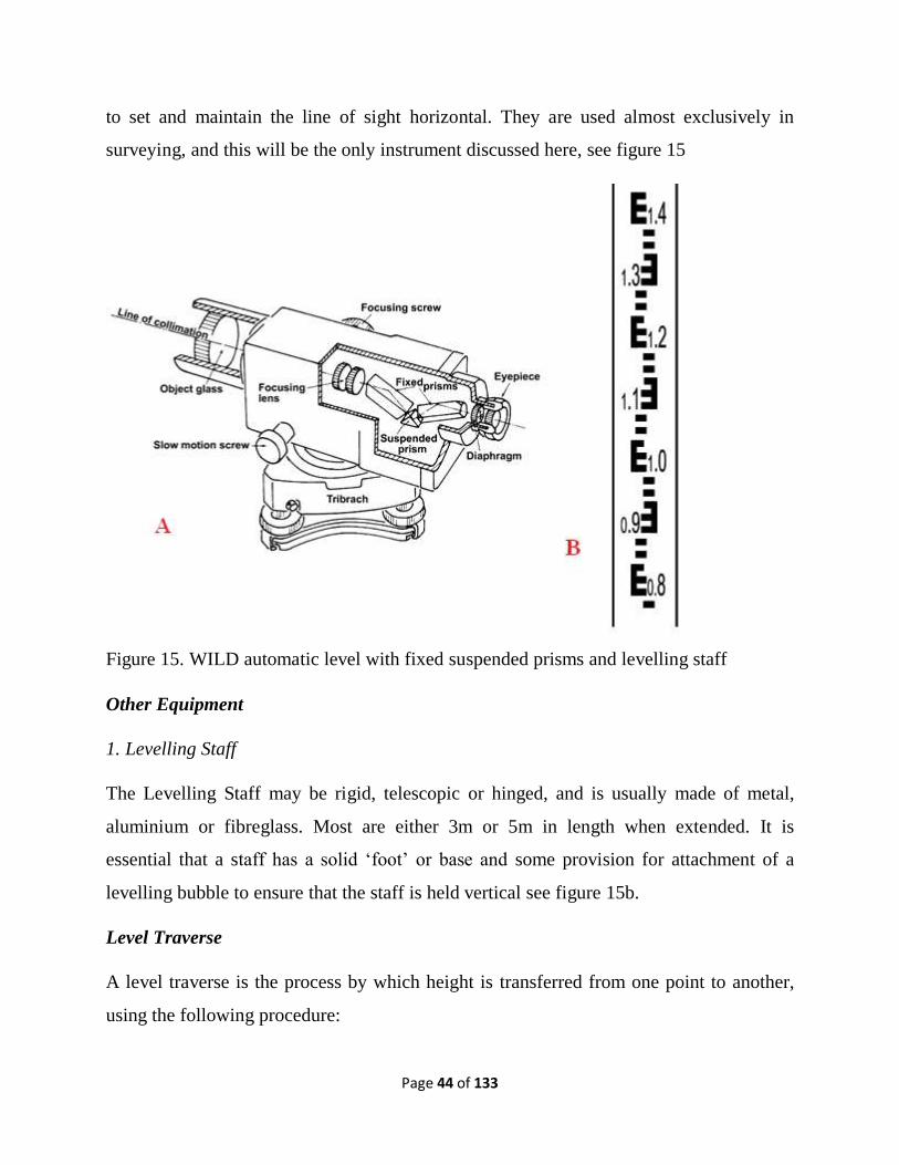
to set and maintain the line of sight horizontal. They are used almost exclusively in

surveying, and this will be the only instrument discussed here, see figure 15

Figure 15. WILD automatic level with fixed suspended prisms and levelling staff

Other Equipment

1. Levelling Staff

The Levelling Staff may be rigid, telescopic or hinged, and is usually made of metal,

aluminium or fibreglass. Most are either 3m or 5m in length when extended. It is

essential that a staff has a solid ‘foot’ or base and some provision for attachment of a

levelling bubble to ensure that the staff is held vertical see figure 15b.

Level Traverse

A level traverse is the process by which height is transferred from one point to another,

using the following procedure:

Page 45 of 133

i. Set up the staff is on a point of known height,

ii. Set up the level instrument and levelled away from the staff, usually no more than

40m,

iii. An initial Backsight reading is taken to the staff,

iv. Then moved the staff to approximately the same distance from the instrument, as it

was for the Backsight reading, in the direction that the traverse is moving. This point is

known as a Change Point.

v. A reading is taken to the staff. This reading is a foresight.

vi. The difference between the two readings will give the difference in height between the

two points. By adding this difference to the known Reduced Level of the first point, the

Reduced Level of the second point (the change point) can be obtained.

vii. The instrument is moved to station 2 on the other side of the staff in the direction of

the traverse.

viii. Without changing the position of the change plate, the staff is rotated so that it faces

towards the instrument.

ix. The procedure of reading a Backsight, moving the staff and reading a Foresight is then

repeated, throughout the traverse, until the required point is reached.

x. Good survey practice requires the traverse to close back onto a Benchmark, so that any

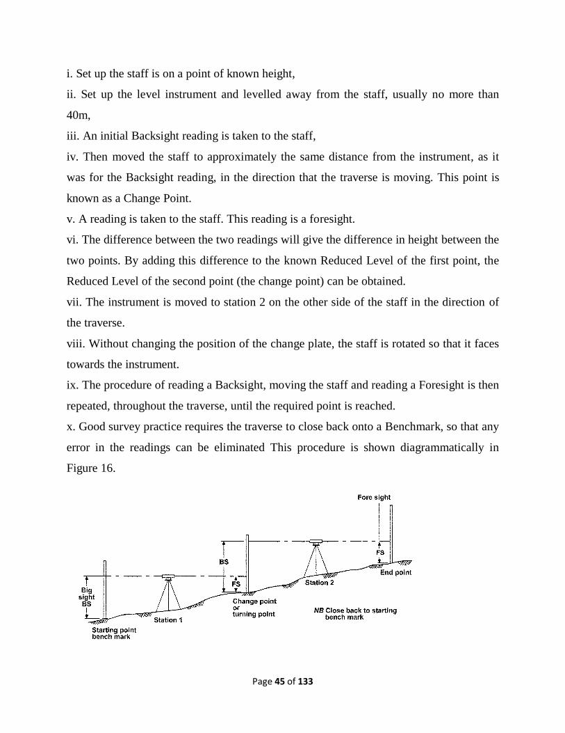
error in the readings can be eliminated This procedure is shown diagrammatically in

Figure 16.

Page 46 of 133

Figure 16. Method of traverse levelling.

Levelling Misclosure

The acceptability of any set of level observations depends upon the magnitude of the

misclosure. This may be determined arbitrarily or calculated from an equation. A major

reason for arbitrarily selecting the maximum acceptable misclosure is the use to which

the Reduced Levels are going to be put; for example:

a. For a precise concrete foundation to support sensitive machinery the maximum

acceptable misclosure may be ±0.002 m.

b. For a sewer the maximum acceptable misclosure may be ±0.005 m.

c. For landscaping the maximum acceptable misclosure may be ±0.20 m.

These accuracy values should not be taken as being absolute as they could vary

depending upon the nature of landscaping, etc. They are only meant to be a guide.

Errors in Levelling

‘Errors’ in levelling will always occur, and may be insignificant or significant enough to

warrant adjustment. These errors come from three main sources:

i. instrumental

ii. personal

iii. environmental.

Instrumental Errors

i. Instrument not adjusted

ii. Staff not vertical

iii. Staff not standardised - worn at the base or at the joins

iv. Tripod legs loose

Personal Errors

i. Incorrect readings

Page 47 of 133

ii. Incorrect bookings

iii. Incorrect addition - the 3 checks not applied

iv. Bubble not centred before each reading

v. Parallax not eliminated

vi. Staff not vertical

vii. Staff not fully extended

viii. Poor change point - staff settles into ground

ix. Poor instrument station - tripod settles into the ground

Environmental Errors

i. Wind - strong wind causes the instrument to vibrate and makes the staff unsteady

ii. Temperature - heat may cause a shimmering effect at ground level near base of staff

and make accurate sightings difficult.

These types of errors may be categorised three under gross, systematic or random.

Gross Errors

These are often caused by the observer or staff-person and are due to carelessness,

inexperience or fatigue. They are shown listed under the heading `Personal Errors'.

Systematic Errors

These are often due to the instrumental defects listed under `Instrumental Errors'. The

most important of these is the collimation error where the whole error for a single shot

(intermediate) is carried over into the staff reading. As previously noted, equalising the

lengths of backsights and foresights eliminates the error. In situations where a large

number of intermediate sights are made, for example building sites, then the two peg test

should be regularly carried out.

Random Errors

These are due mainly to environmental conditions with resulting small errors which tend

to be compensatory. Extreme wind or temperature can cause errors. In windy weather

Page 48 of 133

shelter the instrument, if possible, and keep sights and the staff short. In hot sun reduce

the length of the sights, keeping them at least 0.5 m above ground level to minimise the

effects of refraction.

4.0 Conclusion

Surveying is highly encompassing and very important in practical geography. All spatial

activities must be dimensioned to properly define its location and area coverage. Landed

property beaconing, transportation routes sitting and construction, national and

international boundary demarcations and structural developments require the service of

land surveying, hence their roles in environmental management. Readers will do well by

developing self-interest in the hand-on practical in other to be relevant in environmental

discuss.


i. What is traverse in surveying, and what are the differences between open and close

traverse.

ii. List the three main sources of levelling errors, and discuss two of them in detail. come

from three main sources

iii. What are the two major groups of survey and the areas of operation in the society with

examples.


Michael, M. (2016). Introduction to Surveying. Department of Training and Workforce

Development, Western Australia. Second Edition.

www.vetinfonet.dtwd.wa.gov.au

George, M.C. (2019). Surveyor Reference Manual, 7th Edition – A Complete Reference

Manual for the PS and FS Exam

Raymond, E.P., and Walter, W. (2009). Basic Surveying. Publisher: PHI,

ASIN: B00K7YFVEO

Dixon, R. (2006). Electronic vs. Conventional Surveys. In book: Handbook of Research

on Electronic Surveys and Measurements. DOI: 10.4018/9781591407928.ch011

Page 49 of 133

UNIT 2: AERIAL PHOTOGRAPHY

CONTENT

1.0 Introduction

2.0 Objectives

3.0 Main Content

3.1 Origin of aerial photography and survey

3.2 Use of aircraft and sensors in spatial data collection

3.3 Basic Concepts of Aerial Photography

3.4 Interpretation elements

3.5 Stereoscopic image view

4.0 Conclusion



1.0 Introduction

Aerial photography is an aspect of remote sensing for spatial data inventory with the use

of sensors placed on aircraft platforms at middle altitude. It is a technological

advancement over land surveying as it has some remarkable advantages over the manual

and labour intensive land surveying. Aerial photography is the process of taking

photographs from the air, but there is more to it than simply using a light aircraft or

helicopter and flying up to take photographs. There are many elements to an aerial survey

that must be considered to ensure that the data is useful enough to extrapolate whatever is

being investigated. The utilization and extraction of information from this type of spatial

data source require some professionalism and instrumentation. Although, its utilization is

not without some difficulties in comparison to manually acquired data, but it merits may

outweigh the demerit as will be discussed later.

Page 50 of 133

The major difference between aerial photograph and satellite imagery is the payload and

platform altitude, which in turn influence the type of imagery output utilization in some

specific project. The earlier aerial photographs like the still photograph are the Black-

and-White (Panchromatic) image, and dependent on the camera lens window of operation

in the Electromagnetic System (EMS).

2.0 Objectives

The major objectives of this unit are as given below:

Introduce student to the origin of aerial photography and survey

Expose student to the use of aircraft and sensors in spatial data collection

Student to understand the basic principles of air photography

Student to understand the areas of applications of aerial photography

3.0 Main Content

3.1 Origin of aerial photography and survey

The first aerial photograph that was oblique was taken over a French village in the late

19th century by photographer Gaspar Felix Tournachon who patented the concept of

using aerial photographs to compile maps. It proved much more effective than the time-

consuming ground surveys that the 19th century method. (such as the UK's Ordnance

Survey). George R. Lawrence took aerial photographs of San Francisco in 1906

following the devastating earthquake, but it was not until World War I - when potentially

military applications were foreseen - that a systematic process of taking aerial

photographs would become key to the development of the method.

Archaeologist OGS Crawford pioneered the use of aerial photography for this purpose,

having seen its potential for studying the English landscape. Having experienced the

success of this method of observation, Britain once again used aerial photography during

World War II, employing teams of archaeologists to interpret masses and masses of

photographs taken for aerial reconnaissance purposes. After the war, researchers

welcomed the beginning of the modern movement of landscape studies, natural

Page 51 of 133

processes, archaeological features and treating the landscape as a feature and a monument

in itself. With the arrival of satellite imagery developed through national and

international space agencies, military aerial photography reconnaissance became less

important though not entirely eliminated.

The Cold War and the development of colour photography meant that military

applications continued and it was during this period that wider environmental

applications developed too. Infra-red photography became crucial to vegetation mapping

and also to tracking and identifying diseased plants and trees. The function of taking

landscape photographs at different colours of the spectrum opened up a wide range of

applications across the broadest possible scope of the environment. Better cameras

developed and both the USA and USSR were able to plan reconnaissance trips over key

sites from thousands of feet up in the air. It was then that satellite reconnaissance began

to take over.

Since then, aerial photography has been used extensively in archaeological studies and

later for such wider environmental studies as mapping forests and changes in vegetation

over time, tracking changes in river direction, and depth and planning conservation work

of river systems, and changes to the landscape after natural processes such as landslides.

Its applications are limitless with multiple functions in geology, geography and wider

landscape, rural and urban studies. It is a cheap and effective remote sensing method.

Even today with widely available satellite imagery and public mapping such as Google

Earth, aerial photography remains vital to landscape and other environmental studies.

3.2 Use of aircraft and sensors in spatial data collection

Researchers generally depend on data that most be reliable adequate and more recently

real time to meet urgent needs and current issues. Aerial photography, for example, has

proved more important source of information for ephemeral human and landscape studies

hence its utilization in virtually all facet of human activities as discussed below:

In Archaeology

Page 52 of 133

In archaeology, aerial photography is ideal for locating lost monuments and tracking

features, especially those that are not visible at ground level, those that are under the soil

and cannot be seen on a field work and those that can only be seen under certain

conditions. They are usually discovered through either Crop Marks or Parch Marks:

Seen in summer, crop marks are signs of a subterranean feature that show up as

irregularities in the pattern of crops. Growth of the crop might be stunted due to extant

remains such as stone foundations, or they might be higher than the surrounding crop due

to underlying water systems such as dried up drainage channels or long-gone artificial

water features such as fishponds. Parch marks occur in areas of particularly dry summer.

In some conditions, the crop may simply be a different colour

Soil Marks: Best studied in winter when no crops are growing or grasses have large died

off, both rainy and dry conditions are conducive to picking out buried features. Typically

showing up as darker areas, they can indicate underlying stonework, the outline of

prehistoric features such as barrows and monuments, and ditches. The same issues above

apply - they could be natural or modern features.

Low Profile Monuments:

From the ground they may seem like natural bumps in the ground or be so slight as to be

barely perceptible. From the air, their appearance is far more revealing. On their own

they may or may not look like anything important but if accompanied with the above, can

appear more significant.

In Urban Studies

Urban development and the history of urbanism is a growing niche of landscape studies

which has a wide range of uses through history and archaeology, the history of

cartography, the history of commerce, sociology and even for modern urban planning.

Town developers need to study the impact of expansion and development of urban

centres on the landscape and the impact on the environment. In Climate Change

Page 53 of 133

In global climate change

These global changes are reflected everywhere, and societies and communities are seeing

changes to their local environment. If it isn't river beds drying up, droughts getting

longer, wetter seasons getting wetter and the reduction of inland lakes drying up

completely, one of the most practical applications is tracking of invasive species into

water bodies that just a few years ago would not have provided an adequate environment

for those species. Researchers keep vital records in changes over seasons and years to

track local effects of climate change and risks to local ecosystems. Localised aerial

photographs will highlight the die-off of certain vegetation, or the increase of invasive

species.

In Other Earth Sciences

They can also be used to study the process of natural changes, such as variations in soil

and geology over time as well as changes to the underlying ground that leads to disasters

such as landslides. Aerial survey may not be quite as useful to geologists due to the

relative expense and difficulty in interpretation compared to archaeological applications,

nevertheless it has uses and benefits in that the historical record for changes to the natural

landscape is vital to understanding how the landscape may change in future. Annual

rainfall, whether lower or higher than normal, can have far-reaching consequences. This

is where geology interests in aerial photography are most important. The role of Aerial

photography is increasingly taken over by satellite images and digital mapping of GIS in

recent years. However, it still has the following advantages:

3.3 Basic Concepts of Aerial Photography

Aerial photographs are taken in either oblique or vertical forms and both have different

uses and applications as discussed below. Even today in an age of high quality digital

imaging, black and white (panchromatic) images are preferred - partly because they are

cheaper but also partly because the contrast of black, white and greys makes it easier to

identify features. Most air photo missions are carried out using black and white film.

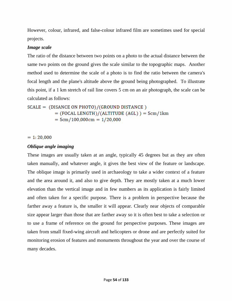
Page 54 of 133

However, colour, infrared, and false-colour infrared film are sometimes used for special

projects.

Image scale

The ratio of the distance between two points on a photo to the actual distance between the

same two points on the ground gives the scale similar to the topographic maps. Another

method used to determine the scale of a photo is to find the ratio between the camera's

focal length and the plane's altitude above the ground being photographed. To illustrate

this point, if a 1 km stretch of rail line covers 5 cm on an air photograph, the scale can be

calculated as follows:

Oblique angle imaging

These images are usually taken at an angle, typically 45 degrees but as they are often

taken manually, and whatever angle, it gives the best view of the feature or landscape.

The oblique image is primarily used in archaeology to take a wider context of a feature

and the area around it, and also to give depth. They are mostly taken at a much lower

elevation than the vertical image and in few numbers as its application is fairly limited

and often taken for a specific purpose. There is a problem in perspective because the

farther away a feature is, the smaller it will appear. Clearly near objects of comparable

size appear larger than those that are farther away so it is often best to take a selection or

to use a frame of reference on the ground for perspective purposes. These images are

taken from small fixed-wing aircraft and helicopters or drone and are perfectly suited for

monitoring erosion of features and monuments throughout the year and over the course of

many decades.

Page 55 of 133

The time of year is vital and in West Africa the dry season may be the best time to take

aerial photographs. There are many reasons for this, not least of all that it is easier to see

features in fields that do not have crops and will not be ploughed for several more

months. Surviving features beneath the surface will often show up darker due to the

shallower levels of soil.

Vertical angle imaging

Taking a photograph straight down over a landscape is the more familiar form of aerial

photograph. It is a plan view so there is no perspective to distort the image. This also

means that it is difficult to read the configuration of the land such as changes in height -

though there is a work around to create 3D image through stereoscopic views, using a

device to examine two at once. This usually gives a good impression of the variation in

the elevation of land. They are taken at regular heights for consistency so it is easier to

compare contexts of a landscape taken on the same day, or many years apart to examine

development.

As a rule, vertical aerial photographs are easier to interpret than oblique photographs

because of the standardised ways in which they are taken - with set scales and at a single

non-arbitrary angle. The same advantages generally apply to vertical as they do for

oblique, but you will lack the perspective, the depth and the 3D effect even with the

weather conditions mentioned above.

Flight line and Image overlap

Aerial survey contractors at the end of a photo mission always plots the location of the

first, last, and every fifth photo centre, along with its roll and frame number, on a

National Topographic System (NTS) map for easy referencing. The small circles along

the straight lines connecting the centre circles represent photo centres to show photos on

the same flight line. While photo overlap is the amount by which one photograph width

covered the previous flight line, which is expressed as a percentage. The photo survey is

designed to acquire 60 per cent forward overlap (between photos along the same flight

line) and 30 per cent lateral overlap (between photos on adjacent flight lines, see figure

17).

Page 56 of 133

Figure 17: Photo flight line and overlaps

Photo Mosaic

Photo mosaic is the agglomeration of series of aerial photographs in such a way that the

detail of one photograph matches all adjacent photographs details. Photo Mosaics are

necessary when carrying out a project over a large area using large scale aerial

photographs. This operation can be performed in three ways (uncontrolled mosaics, semi-

controlled mosaics and controlled mosaics) as discussed below:

Controlled Mosaics

a. Clients must supply a base map as well as a minimum of three (3) ground

control points per hard copies.

b. The hard copies are tone-matched and rectified to fit the map base.

Semi-Controlled Mosaics

a. The hard copies used in the mosaic are tone-matched but not rectified.

b. Hard copies are laid down to fit a map base of the same scale.

c. Title and scale may be added.

Uncontrolled Mosaics

a. Hard copies are laid out so as to join together in a "best fit" scenario.

b. Hard copies may be tone-matched.

3.5 Stereoscopic image view

Before an interpreter commences the reading of the photo, the concept of stereoscopy

must be understood. Usually a stereoscope is used for image interpretation. There are

Page 57 of 133

several types of stereoscope, for example, portable lens stereoscope, stereo mirror scope

(see Fig. 18) stereo zoom transfer scope etc. The process of stereoscopy for aerial

photography is as follows.

i. Mark the centre of both aerial photographs, called the principal point.

ii. The principal point of the right image should be plotted in its position on the left

image, and at the same time the principal point of the left image should be plotted on the

right image.

iii. These principal points and transferred points should be aligned along a straight line,

called the base line, with an appropriate separation (normally 25-30 cm in the case of a

stereo mirror scope.

iv. By viewing through the binoculars a stereoscopic model can now be seen.

v. A pair of stereoscopic photographs or images can be viewed stereoscopically by

looking at the left image with the left eye and the right image with the right eye. This is

called stereoscopy.

Stereoscopy is based on Porro-Koppe's Principle that the same light path will be

generated through an optical system if a light source is projected onto the image taken by

an optical system

The principle will be realized in a stereo model if a pair of stereoscopic images is

reconstructed using the relative location or tilt at the time the photography was taken.

Such an adjustment is called relative orientation in photogrammetric terms. The eye-base

and the photo-base must be parallel in order to view at a stereoscopic model, as shown in

the Fig. 18.

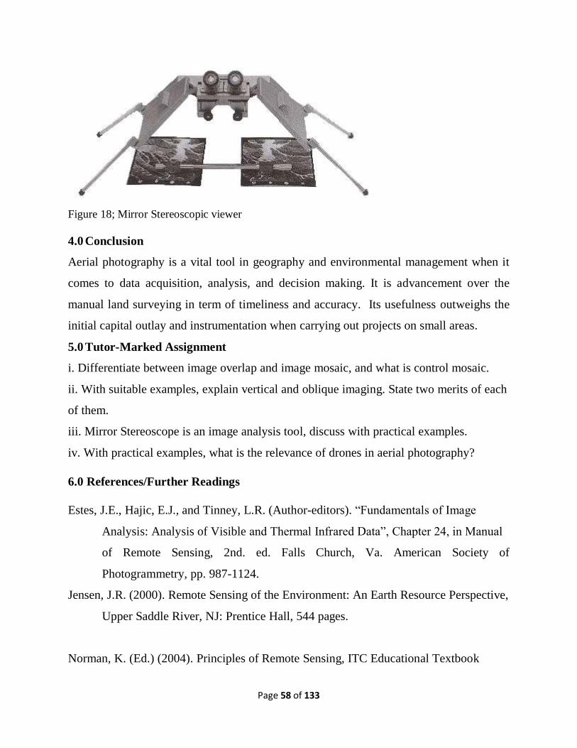
Page 58 of 133

Figure 18; Mirror Stereoscopic viewer

4.0 Conclusion

Aerial photography is a vital tool in geography and environmental management when it

comes to data acquisition, analysis, and decision making. It is advancement over the

manual land surveying in term of timeliness and accuracy. Its usefulness outweighs the

initial capital outlay and instrumentation when carrying out projects on small areas.


i. Differentiate between image overlap and image mosaic, and what is control mosaic.

ii. With suitable examples, explain vertical and oblique imaging. State two merits of each

of them.

iii. Mirror Stereoscope is an image analysis tool, discuss with practical examples.

iv. With practical examples, what is the relevance of drones in aerial photography?


Estes, J.E., Hajic, E.J., and Tinney, L.R. (Author-editors). “Fundamentals of Image

Analysis: Analysis of Visible and Thermal Infrared Data”, Chapter 24, in Manual

of Remote Sensing, 2nd. ed. Falls Church, Va. American Society of

Photogrammetry, pp. 987-1124.

Jensen, J.R. (2000). Remote Sensing of the Environment: An Earth Resource Perspective,

Upper Saddle River, NJ: Prentice Hall, 544 pages.

Norman, K. (Ed.) (2004). Principles of Remote Sensing, ITC Educational Textbook

Page 59 of 133

Series, 250p.

Paine, D.E (1981). Aerial Photography and Image Interpretation for Resource

Management, New York, John Wiley and Sons, 571 p.

Page 60 of 133

UNIT 3: SATELLITE IMAGERY

CONTENT

1.0 Introduction

2.0 Objectives

3.0 Main Content

3.1 Satellite and orbits.

3.2 Remote sensing system and radiant energy

3.3 Basic wavelength regions and application

3.4 Common remote sensing sensors

3.5 Software for satellite image processing and analysis.

4.0 Conclusion



1.0 Introduction

Satellite Imageries are images acquired through remote sensing approaches which are the

science and art of obtaining information about an object, area or phenomenon through an

analysis of the data acquired by a device which is not in contact with the object, area or

phenomenon under investigation. It is further required that such sensing may be achieved

in the absence of any matter in the intervening space between the object and the observer.

Consequently, the information about the object, area or any phenomenon must be

available in a form that can be impressed on a carrier vacuum. The information carrier, or

communication link, is electromagnetic energy. Remote sensing data basically consists of

wavelength intensity information acquired by collecting the electromagnetic radiation

leaving the object at specific wavelength and measuring its intensity. Remote sensing of

earth's environment comprises measuring and recording of electromagnetic energy

reflected from or emitted by the planet's surface and atmosphere from a· vantage point

above the surface, and relating of such

Page 61 of 133

Space borne sensors are currently used to assist in scientific and socioeconomic activities

like weather prediction, crop monitoring, mineral exploration, waste land mapping,

cyclone warning, water resources management, and pollution detection. All this has

happened in a short period of time. The quality of analysis of remote sensing data and the

varied types of applications to which the science of remote sensing is being put to use are

increasing enormously as new and improved spacecraft are being placed into the earth's

orbit. An attempt is made to classify the satellites into three types, namely, earth

resources satellites, meteorological satellites, and satellites carrying microwave sensors.

This classification is not rigid. For instance, most of the meteorological satellites are also

capable of sensing the resources of the earth.

2.0 Objectives

The objectives of this subunit are as stated below:

To further exposed the student to advanced spatial data acquisition techniques

Acquit the student with satellite imageries and its characteristics

To reveal to students the merit and demerits of the various spatial data acquisition

techniques

To expose student to basic remote sensing activities and platforms, and

To expose student to basic sensors and Electromagnetic Spectrum windows

3.0 Main Content

3.1 Satellite and Orbit

Remote sensing satellites are space born vehicles that are used to carry out space

exploration of the planets including our own earth. They are meant to acquire and relay

communications signals or transmit scientific data to their ground receiving stations at the

home country. Each satellite in the outer space are owned by individual countries in

accordance to the global regulatory bodies in term of orbiting operation positioning.

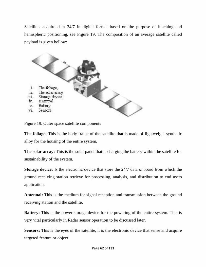
Page 62 of 133

Satellites acquire data 24/7 in digital format based on the purpose of lunching and

hemispheric positioning, see Figure 19. The composition of an average satellite called

payload is given bellow:

Figure 19. Outer space satellite components

The foliage: This is the body frame of the satellite that is made of lightweight synthetic

alloy for the housing of the entire system.

The solar array: This is the solar panel that is charging the battery within the satellite for

sustainability of the system.

Storage device: Is the electronic device that store the 24/7 data onboard from which the

ground receiving station retrieve for processing, analysis, and distribution to end users

application.

Antennal: This is the medium for signal reception and transmission between the ground

receiving station and the satellite.

Battery: This is the power storage device for the powering of the entire system. This is

very vital particularly in Radar sensor operation to be discussed later.

Sensors: This is the eyes of the satellite, it is the electronic device that sense and acquire

targeted feature or object

Page 63 of 133

Satellite orbit is the imaginary path that the satellite follows around the earth at a defined

altitude and hemisphere. This is very important to the global coordinating body to avoid

collision of spacecrafts. It is pre-determined at the point of satellite manufacturing before

lunching at lunching stations Satellite orbit can be grouped into two according to their

altitude, geographical position, and type of data acquisition. These groupings are Polar

and Geostationary orbiting satellites as discussed below:

Polar orbiting satellite

Near the earth, polar orbiting also called sun-synchronous satellites are located at a much

lower altitude, generally a few hundred to a few thousand kilometres. In the case of this

type of satellites, the time at which the satellite revisits a given location is the same on

each occasion. This is very useful for visible and infrared observations, since the level of

solar illumination can be chosen. Biological and environmental studies, for example,

require specific timings for the collection of data. Fig 20 illustrates the principles of a

sun-synchronous orbit. The angle between the orbital plane and the earth's equatorial

plane is termed the inclination of the orbit. Changes in the orbit are due largely to

precision caused mainly by the slightly non-spherical shape of the earth. Landsat, IRS

and SPOT are some of the satellites which have this kind of orbit.

Figure 20; Sun synchronous orbiting satellite.

Some earth observing platforms are not in near polar, sun-synchronous orbits like the

space shuttle that has an equatorial orbit. Thus, the orbit selected for a particular satellite

determines not just the time taken to complete one orbit (temporal resolution) but also the

Page 64 of 133

nature of the relationships between the satellite and solar illumination direction.

Therefore illumination and observation angle are very important parameter on which the

precision of satellite data depends.

Many satellite systems observe at the nadir (directly below the satellite viewing angle =

0°), and this is especially valuable for imaging systems since distortion is reduced if the

image and object planes are parallel. True polar orbiting satellite, however, observe at

non-zero viewing angles. This is usually to exploit the dependence on incidence angle of

the emissivity or reflectivity of the surface, for which a physical model may exist.

Observation away from nadir can thus assist in the discrimination of one target material

from another or the measurement of some physical property of the target material.

Geostationary orbiting satellite

Geostationary are stationary with respect to the earth and are at an altitude of about

36000 km above a point on the equator, that is, geostationary satellites maintain a fixed

location with respect to the earth's surface. Conversely, a satellite in a low polar orbit

traces out a curving path over the earth's surface, as a consequence of the satellite's

orbital motion and precision and of the earth's rotation about its axis. This path (the sub

satellite track) wraps itself round the earth from east to west like a ball of string,

oscillating between the equal north and south latitudes in a pattern set by the inclination

of the orbit. The oath may close up on itself if the orbital parameters (inclination, height

and eccentricity) are suitably chosen, in which case the satellite will revisit a given

location at regular intervals. This interval may in general be any integral number of days,

though other constraints on the orbital parameters may limit the choice.

The point where the satellite, travelling northwards, passes directly over the equator is

called the ascending node. The descending node describes the southward crossing

(Stewart, 1985 and Rees, 1990). Owing to their immense distance from the earth, high

resolution imaging is difficult, hence used for meteorological and communication

activities. INSAT, GOES and METEOSAT are some of the satellites under this category.

Page 65 of 133

3.2 Remote sensing system and radiant energy

The remote sensing system is the components and operation of the system that are used to

acquire data remotely. The system is composing of the following:

i. The power source

ii. The interaction

iii. The sensors

iv. The target objects

The power source

The power source for remote sensing operation is generally the radiant energy from the

Sun. The planet earth receives its illumination from the Sun as it rotates and revolves

round it. The satellite sensor in turn records the modified radiant energy from its target.

The radiant energy interaction

The incoming solar radiant energy from the sun interact with the components of the

atmosphere as it passes through it and also interact with earth features as discussed

below:

Atmospheric interaction;

The composition of the atmosphere at a given point in place and time is a function of the

season of the year and human activities. The atmosphere comprises of air gasses that

contain water vapour, and aerosols. When electromagnetic radiation interacts with these,

it may be absorbed. Reflected, diffuses, or back scattered. When the atmosphere is

saturated with water vapour, absorption takes place; when dry aerosols are more,

reflectance and diffusion takes place. Back scatter may occur a little in the atmosphere

depending on the air mass content.

Page 66 of 133

Surface interaction

Radiant energy interaction with the earth surface feature is of more importance to remote

sensing system because, this is what actually affect the returns of wavelength recorded by

sensors onboard satellites. Generally, about 51% of the in-coming radiant energy from

the Sun reaches the Earth's surface features, and of this total, 4% is reflected back into the

atmosphere and 47% is absorbed by the Earth's surface to be re-radiated later in the form

of thermal radiation. Although, there is great variation in the way the different features on

the Earth's surface reflect or absorb in-coming radiation. In general, living things do more

of absorption than none living things as discuss below.

Absorption: At the earth surface, features like water bodies, tick tree canopy; black

surfaces and dense matter etc do more of absorption of the incoming radiant energy.

Reflection: Smoot and glossy surfaces like glaze artificial structures, aluminium

surfaces, bright painted surfaces and loose coarse materials like sand bare surfaces.

Diffusion: This is the random movement of radiant energy from one site in a medium to

another, resulting in complete mixing the whole matter. In this situation much of the

incoming energy is lost to the remote sensor record.

Backscattered: Polygonal rough earth features generally scatter incoming radiant

energy. This can be natural or artificial features like of the architectural structures and

dome-shaped surfaces.

Black Body

Every object or matter receiving incoming radiant energy radiates unique radiant flux

depending on the object mass and density. This radiation is called thermal radiation

because it mainly depends on temperature. A black body is matter that absorbs all

electro-magnetic energy, incident upon it and does not reflect nor transmit. A black body

shows the maximum radiation as compared with other matter. Therefore, a black body is

called a perfect radiator.

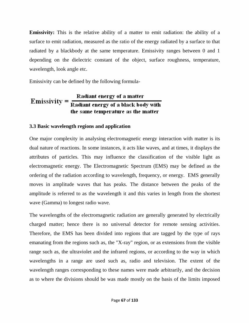
Page 67 of 133

Emissivity: This is the relative ability of a matter to emit radiation: the ability of a

surface to emit radiation, measured as the ratio of the energy radiated by a surface to that

radiated by a blackbody at the same temperature. Emissivity ranges between 0 and 1

depending on the dielectric constant of the object, surface roughness, temperature,

wavelength, look angle etc.

Emissivity can be defined by the following formula-

3.3 Basic wavelength regions and application

One major complexity in analysing electromagnetic energy interaction with matter is its

dual nature of reactions. In some instances, it acts like waves, and at times, it displays the

attributes of particles. This may influence the classification of the visible light as

electromagnetic energy. The Electromagnetic Spectrum (EMS) may be defined as the

ordering of the radiation according to wavelength, frequency, or energy. EMS generally

moves in amplitude waves that has peaks. The distance between the peaks of the

amplitude is referred to as the wavelength it and this varies in length from the shortest

wave (Gamma) to longest radio wave.

The wavelengths of the electromagnetic radiation are generally generated by electrically

charged matter; hence there is no universal detector for remote sensing activities.

Therefore, the EMS has been divided into regions that are tagged by the type of rays

emanating from the regions such as, the "X-ray" region, or as extensions from the visible

range such as, the ultraviolet and the infrared regions, or according to the way in which

wavelengths in a range are used such as, radio and television. The extent of the

wavelength ranges corresponding to these names were made arbitrarily, and the decision

as to where the divisions should be was made mostly on the basis of the limits imposed

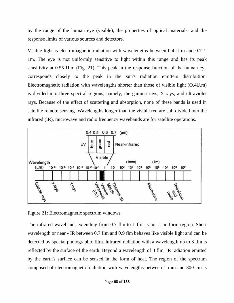
Page 68 of 133

by the range of the human eye (visible), the properties of optical materials, and the

response limits of various sources and detectors.

Visible light is electromagnetic radiation with wavelengths between 0.4 IJ.m and 0.7 !-

1m. The eye is not uniformly sensitive to light within this range and has its peak

sensitivity at 0.55 IJ.m (Fig. 21). This peak in the response function of the human eye

corresponds closely to the peak in the sun's radiation emitters distribution.

Electromagnetic radiation with wavelengths shorter than those of visible light (O.4lJ.m)

is divided into three spectral regions, namely, the gamma rays, X-rays, and ultraviolet

rays. Because of the effect of scattering and absorption, none of these bands is used in

satellite remote sensing. Wavelengths longer than the visible red are sub-divided into the

infrared (IR), microwave and radio frequency wavebands are for satellite operations.

Figure 21: Electromagnetic spectrum windows

The infrared waveband, extending from 0.7 flm to 1 flm is not a uniform region. Short

wavelength or near - IR between 0.7 flm and 0.9 flm behaves like visible light and can be

detected by special photographic film. Infrared radiation with a wavelength up to 3 flm is

reflected by the surface of the earth. Beyond a wavelength of 3 flm, IR radiation emitted

by the earth's surface can be sensed in the form of heat. The region of the spectrum

composed of electromagnetic radiation with wavelengths between 1 mm and 300 cm is

Page 69 of 133

called the microwave band and radiation at these wavelengths can penetrate the clouds.

The microwave band is thus a valuable region for remote sensing. Beyond the microwave

region is the radioband of very long wavelengths used in certain radar applications. The

electromagnetic wavebands with their utility in remote sensing are described in Table 1.

The electromagnetic wavebands with their utility.

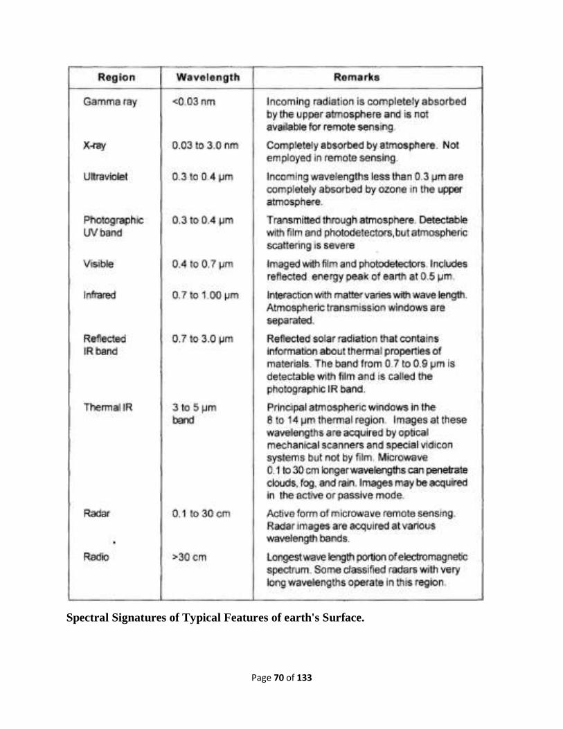
Page 70 of 133

Spectral Signatures of Typical Features of earth's Surface.

Page 71 of 133

Every object on the surface of the earth has its unique spectral reflectance. Figure 22

shows the average spectral reflectance curves for three typical earth's features: vegetation,

soil and water. The spectral reflectance curves for vigorous vegetation manifests the

"Peak-and-valley" configuration. The valleys in the visible portion of the spectrum are

indicative of pigments in plant leaves. Dips in reflectance (Figure 22) that can be seen at

wavelengths of 0.65 !J.m, 1.4 !J.m and 1.9 !J.m, are attributable to absorption of water by

leaves. The soil curve shows a more regular variation of reflectance. Factors that

evidently affect soil reflectance are moisture content, soil texture, surface roughness, and

presence of organic matter. The term spectral signature can also be used for spectral

reflectance curves. Spectral signature is a set of characteristics by which a material or an

object may be identified on any satellite image or photograph within the given range of

wavelengths. Sometime&, spectral signatures are used to denote the spectral response of

a target.

The characteristic spectral reflectance curve Fig. 22 for water shows that from about

0.5!J.m, a reduction in reflectance with increasing wavelength, so that in the near infrared

range, the reflectance of deep, clear water is virtually a zero (Mather, 1987). However,

the spectral reflectance of water is significantly affected by the presence of dissolved and

suspended organic and inorganic material and by the depth of the water body.

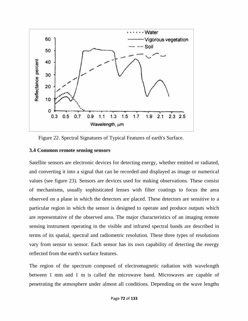
Page 72 of 133

Figure 22. Spectral Signatures of Typical Features of earth's Surface.

3.4 Common remote sensing sensors

Satellite sensors are electronic devices for detecting energy, whether emitted or radiated,

and converting it into a signal that can be recorded and displayed as image or numerical

values (see figure 23). Sensors are devices used for making observations. These consist

of mechanisms, usually sophisticated lenses with filter coatings to focus the area

observed on a plane in which the detectors are placed. These detectors are sensitive to a

particular region in which the sensor is designed to operate and produce outputs which

are representative of the observed area. The major characteristics of an imaging remote

sensing instrument operating in the visible and infrared spectral bands are described in

terms of its spatial, spectral and radiometric resolution. These three types of resolutions

vary from sensor to sensor. Each sensor has its own capability of detecting the energy

reflected from the earth's surface features.

The region of the spectrum composed of electromagnetic radiation with wavelength

between 1 mm and 1 m is called the microwave band. Microwaves are capable of

penetrating the atmosphere under almost all conditions. Depending on the wave lengths

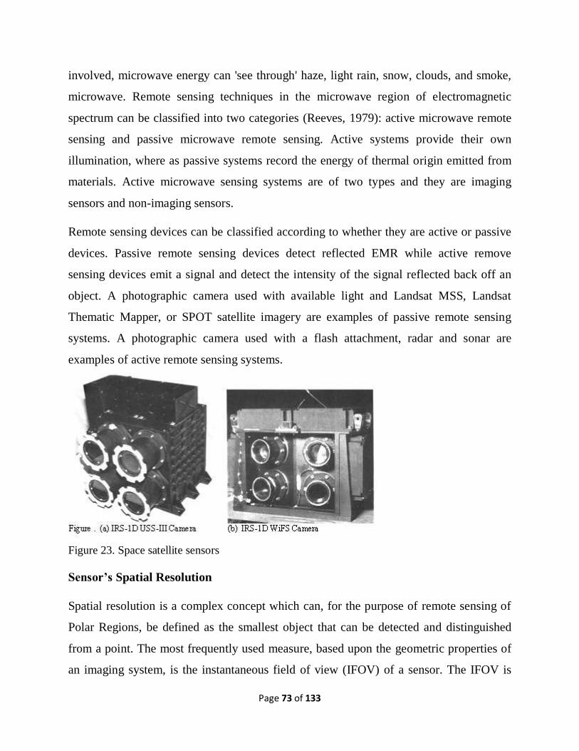
Page 73 of 133

involved, microwave energy can 'see through' haze, light rain, snow, clouds, and smoke,

microwave. Remote sensing techniques in the microwave region of electromagnetic

spectrum can be classified into two categories (Reeves, 1979): active microwave remote

sensing and passive microwave remote sensing. Active systems provide their own

illumination, where as passive systems record the energy of thermal origin emitted from

materials. Active microwave sensing systems are of two types and they are imaging

sensors and non-imaging sensors.

Remote sensing devices can be classified according to whether they are active or passive

devices. Passive remote sensing devices detect reflected EMR while active remove

sensing devices emit a signal and detect the intensity of the signal reflected back off an

object. A photographic camera used with available light and Landsat MSS, Landsat

Thematic Mapper, or SPOT satellite imagery are examples of passive remote sensing

systems. A photographic camera used with a flash attachment, radar and sonar are

examples of active remote sensing systems.

Figure 23. Space satellite sensors

Sensor’s Spatial Resolution

Spatial resolution is a complex concept which can, for the purpose of remote sensing of

Polar Regions, be defined as the smallest object that can be detected and distinguished

from a point. The most frequently used measure, based upon the geometric properties of

an imaging system, is the instantaneous field of view (IFOV) of a sensor. The IFOV is

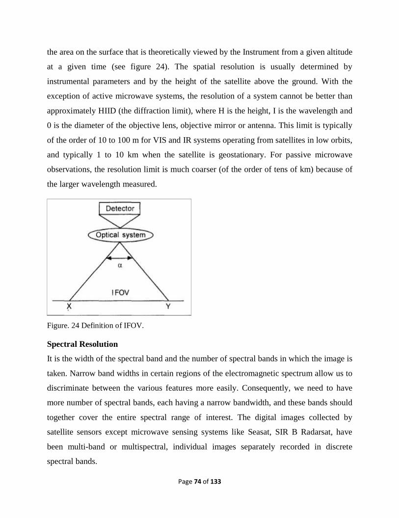
Page 74 of 133

the area on the surface that is theoretically viewed by the Instrument from a given altitude

at a given time (see figure 24). The spatial resolution is usually determined by

instrumental parameters and by the height of the satellite above the ground. With the

exception of active microwave systems, the resolution of a system cannot be better than

approximately HIID (the diffraction limit), where H is the height, I is the wavelength and

0 is the diameter of the objective lens, objective mirror or antenna. This limit is typically

of the order of 10 to 100 m for VIS and IR systems operating from satellites in low orbits,

and typically 1 to 10 km when the satellite is geostationary. For passive microwave

observations, the resolution limit is much coarser (of the order of tens of km) because of

the larger wavelength measured.

Figure. 24 Definition of IFOV.

Spectral Resolution

It is the width of the spectral band and the number of spectral bands in which the image is

taken. Narrow band widths in certain regions of the electromagnetic spectrum allow us to

discriminate between the various features more easily. Consequently, we need to have

more number of spectral bands, each having a narrow bandwidth, and these bands should

together cover the entire spectral range of interest. The digital images collected by

satellite sensors except microwave sensing systems like Seasat, SIR B Radarsat, have

been multi-band or multispectral, individual images separately recorded in discrete

spectral bands.

Page 75 of 133

Multispectral imaging refers to viewing a given area in several narrow bands to obtain

better identification and classification of objects. Multistage imaging refers to the

observations of the same area from different positions of the platforms (stereoscopic

data). Multistage imaging refers to the observations made over the same area on different

dates to monitor the objects like crop growth. This is also called temporal resolution. The

term spectral resolution refers to the width of the spectral bands. Spectral resolution can

be explained by considering two points, (i) the position of the spectrum, width and

number of spectral bands will determine the degree to which individual targets can be

determined on the multispectral image, and (ii) the use of multispectral imagery can lead

to a higher degree of discriminating power than any single band taken on its own.

Broadly, all the imaging sensor systems are classified based on technical components of

the system and the capability of the detection by which the energy reflected by the terrain

features is recorded. The classification scheme is (a) Multispectral imaging sensor

systems (b) Thermal remote sensing systems, and (c) Microwave radar sensing systems.

The multispectral or multiband imaging systems may use conventional type cameras or a

combination of them, along with filters for the various bands in the visible part in the

scanning system of multiband imaging.

Radiometric Resolution

It is the capability to differentiate the spectral reflectance/emittance between various

targets. This depends on the number of quantisation levels within the spectral band. In

other words, the number of bits of digital data in the spectral band or the number of gray

level values, will decide the sensitivity of the sensor. It is the smallest difference in

exposure that can be detected in a given film analysis. It is also the ability of a given

sensing system to discriminate between density levels.

Thermal Sensing Systems

Thermal scanner is one of the most important thermal sensing systems, a particular kind

of across track multispectral scanner which senses in the thermal portion of the

electromagnetic spectrum by means of inbuilt detectors. These systems are restricted to

Page 76 of 133

operating in either 3 to 5 I-lm or 8 to 14 I-lm range of wavelengths. The operation and the

efficiency of this type of scanning systems are based on the characteristics of the

detectors. Quantum or photon detectors are typically used to detect the thermal radiation.

These detectors operate on the principle of direct interaction between photons of radiation

incident on them and the energy levels of electrical charge carriers within the detector

material.

The RADAR

Radio Detection and Ranging (RADAR) is an active microwave sensing system which

transmits electromagnetic radiation of wave length in the centimetre range as a source of

illumination (self-illumination) to detect remote targets. Most imaging sensor or imaging

radars used for remote sensing are Side Looking Airborne Radar (SLAR). The radar is an

acronym derived from Radio Detector and Ranging. These imaging radars are divided

into two categories. The first category is real aperture, and the second one is synthetic

aperture systems. In the real aperture system, resolution is determined by the actual beam

Electro-optical scanners used in both airborne and satellite remote sensing are somewhat

similar to digital cameras in that they use an array of electronic sensors, in combination

with mirror/lens optical devices to scan a scene and record an image. Each sensor in the

array produces an electrical signal for each wavelength detected. The electrical signals

can be recorded on magnetic tape. In the case of satellite sensors, the continuous

electrical signals are usually converted into digital numbers representing up to 256 gray

levels before being transmitted to Earth-based receiving stations. Optical-electrical

scanners offer the potential of real time data acquisition

In synthetic aperture radar (SAR) imaging, microwave pulses are transmitted by an

antenna towards the earth surface. The microwave energy scattered back to the spacecraft

is measured. The SAR makes use of the radar principle to form an image by utilising the

time delay of the back scattered signals

Page 77 of 133

Multispectral Imaging Sensor Systems

A multispectral scanner (MSS) operates on the same principle of selective sensing in

multiple spectral bands, but such instruments can sense in many more bands and over a

great range of the electromagnetic spectrum. Because of the advancement in utilising

electronic detectors, MSS can extend the range of sensing from 0.3 flm to 14 flm. Further

MSS can sense in very narrow bands. Multispectral scanner images are acquired by

means of two basic process: across-track and along-track scanning. Multispectral scanner

systems build up two-dimensional images of the terrain for a swath beneath the platform.

Across-track systems are also called whisk broom scanner systems. This type of scanning

system scans the terrain along scanlines that are right angles to the direction of the space

borne/airborne platform.

The second type of multispectral scanning system is along-track scanning system or push

broom systems. This type of scanner record multiband image data along a swath beneath

an aircraft. As the aircraft/spacecraft advances in the forward direction, the scanner scans

the earth with respect to the designed swath to build a two-dimensional image by

recording successive scan lines that are oriented at right angles to the direction of the

aircraft/spacecraft, (see figure 25).

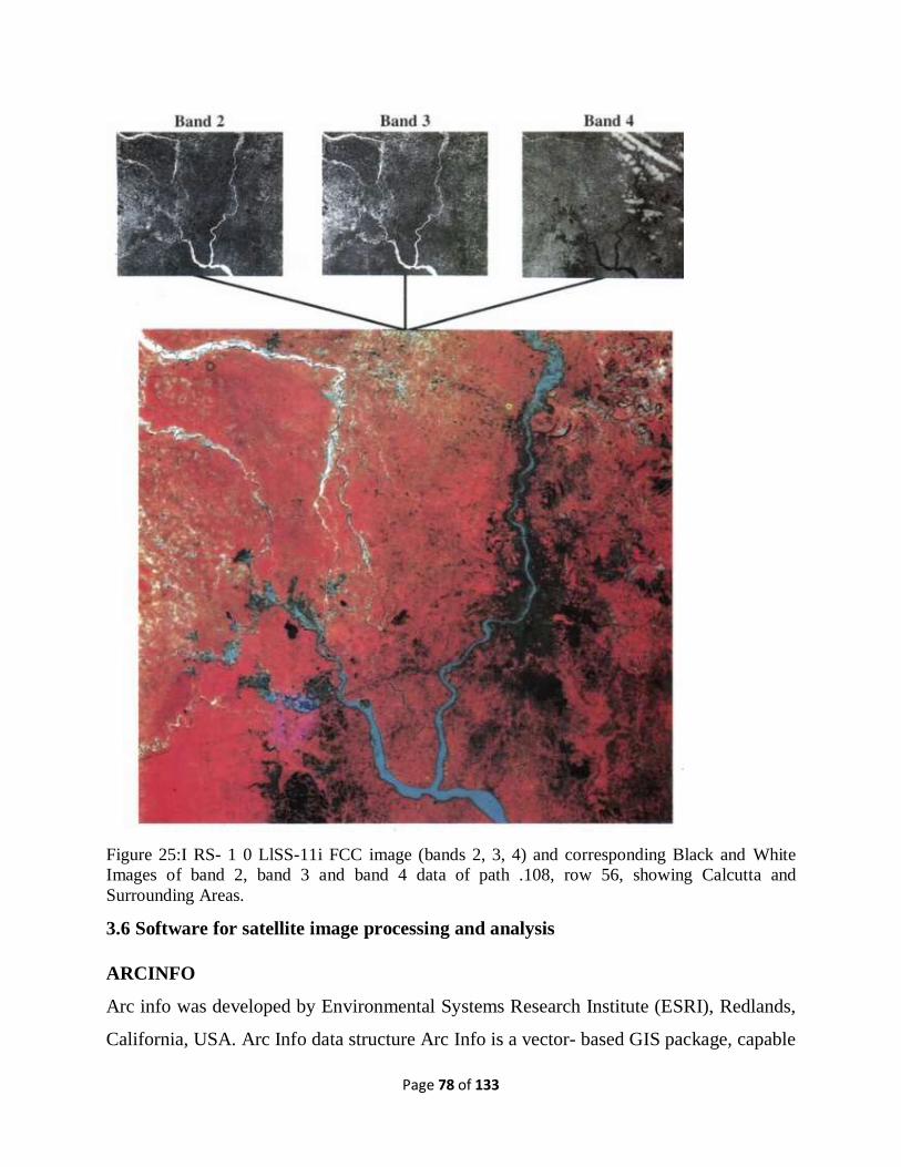
Page 78 of 133

Figure 25:I RS- 1 0 LlSS-11i FCC image (bands 2, 3, 4) and corresponding Black and White

Images of band 2, band 3 and band 4 data of path .108, row 56, showing Calcutta and

Surrounding Areas.

3.6 Software for satellite image processing and analysis

ARCINFO

Arc info was developed by Environmental Systems Research Institute (ESRI), Redlands,

California, USA. Arc Info data structure Arc Info is a vector- based GIS package, capable

Page 79 of 133

of handling both spatial and non-spatial data. It organizes geographical data using vector

topological models and non-spatial data using relational models in a DBMS. The arc

node and polygon topology are organized to identify points, lines, and polygon relations.

The cartographic data are then linked to the attribute data through a link item. Arc Info

functionalities: Arc Info has a wide range of functions which have been developed based

on a tool-box concept -where each function can be visualized as a tool and having a

specific utility.

IDRISI GIS

IDRISI GIS: has been developed by Clark University, USA. It has advanced features like

import /export capabilities, a new digitizing module, and image processing tools. It runs

on PC's. Manipulation and import of vector data is supported.

ERDAS

ERDAS (Earth Resources Data Analysis System) is the mapping software company

specializing in Geographic Imaging Solutions since 1978. The company is world leader

in highly customizable, easy-to-learn and-use Geographic Imaging software. The

software is precisely for Visualization. The essentials of this software are vector module,

virtual GIS, NIFT, radar module.

GRASS

A public domain UNIX package. It has several image processing tools and good support

for spatial statistics and analysis. It has strong support for raster/vector integration.

GRASS is mainly used for hydrologic / watershed modelling applications.

EASI/PACE

It is a remote sensing software developed by PCI Geomatics, Ontario, Canada. It is

designed for Remote Sensing, Image Processing, Data Visualization and GIS Support.

The functional components are Image Works; Xpace; GCP works, EASI; PCI Modeler

and ACE.

Page 80 of 133

Maplnfo

Has very good spatial data handling capabilities. It supports dBase and also has its own

data manager.

PAMAPGIS

The PAMAP GIS is a product of PAMAP Graphics Limited, Canada, integrated group of

software designed for open 'system environment. This package is modular and designed

to address the wide range of mapping and analysis requirements of the natural resource

sector. PAMAP data structure PAMAP adopts an integrated raster as well as vector

representation of the

spatial elements. It uses vectors for data capture and storage and rasters for analysis

purposes.

SPANS

Spatial Analysis System (SPANS) is a GIS package developed by TYOAC Technologies;

Canada has a powerful modelling function for applications. SPANS data Structure: It

adopts a mixed vector tessellation approach to the GIS and has developed the region -

quad tree data structure. It has the ability to read and process vector and raster formats

used by other GISs.

ISROGIS

This is developed by Indian Space Research Organization. ISRO data structure: it adopts

PM quadtree data structure, which is edge based structure that decomposes the vectors in

map into quads, and then organized using the vector structure.

ENVI

The Environment for Visualizing Images (ENVI) provides the most complete set of

image processing tools and functions available for our land cover analysis using Landsat

TM and SPOT data. It runs exactly the same way on-windows, Unix and Macintosh

systems. Its orthorectification features help correct aircraft or satellite position,

topography and other camera effects.

Page 81 of 133

4.0 Conclusion

Remote sensing and satellite imagery system is an advance technology in spatial data

acquisition and analysis that far ahead of the earlier land surveying. The levels of

detailing and real time data acquisition favoured the present day socio-economic

dynamism and globalization of things. When it comes to major projects implementation

and policy formation, remotely sensed data gives the best result.


i. What remote sensing satellites and their payload components.

ii. With suitable examples, discuss the operational activities of the radiant energy

interaction with the atmosphere.

iii. List and discuss five (5) GIS software indicating their areas of uniqueness.

iv. What is the relevance of Electromagnetic Spectrum (EMS) in space data acquisition,

and the major uniqueness of RADAR sensor above others.


Robert, M. (1991). Satellite Remote Sensing of Polar Regions, CBS Publishers, New

Delhi.

Seigal, B.S., and Alan, R.G. (eds) (1980). Remote Sensing in Geology, John Wiley and

Sons, New York.

Stewart, R. (1985). Methods of Satellite Oceanography, University of California Press,

Berkeley California.

Wolfe., W.L., and Zissis, G.J. (1989). The Infrared Handbook. The Infrared Information

Analysis Center, Environmental Research Institute of Michigan, USA.




Series, 250p.

Page 82 of 133

MODULE THREE

ELEMENTARY MAP AND IMAGE INTERPRETATION

UNIT 1: TYPES OF MAP SCALE

CONTENT

1.0 Introduction

2.0 Objectives

3.0 Main Content

3.1: Types of map scales.

3.2: Conventional signs

3.3: Image interpretation elements

3.4: Map reduction and enlargement

3.5: Map digitization (On-screen and Tablet)

4.0 Conclusion



1.0 Introduction

Manual map reading and image interpretation of aerial photography is among the most

commonly used methods for ecosystem classification and production of inventory maps

for resource management (Leckie and Gillis 1995; Thompson et al. 2007). Map

interpretation involves the identification and studying of factors that explain the causal

relationship among several features as revealed by the feature symbols shown on the

map. For instance, the distribution of natural and secondary vegetation covers in relation

to human developmental activities or cultivated land against the background of landform

and drainages. Conventional interpretation consists of polygon delineation and

classification (Avery and Berlin 1992; Paine and Kiser 2003). Manual interpretation uses

Page 83 of 133

a “convergence of evidence” approach in which many traits (tone or colour, shape, size,

texture, pattern, shadow, local topography, and neighbouring contextual cues) are

considered in combination. Such characteristics are used to delineate boundaries and

classify a homogenous area or forest stand.

Manual interpretation can be subjective and difficult to replicate; thus yielding

inconsistent results (Wulder et al. 2008). Manual interpretation can be laborious and

expensive (Green 2000), resulting in infrequent updates. Furthermore, re-examination of

forest inventory interpretations has yielded unexpected accuracies. For example, field

reconnaissance evaluating Ontario's Forest Resource Inventory found approximately 30%

of stands were misclassified for conifer, deciduous, or mixed classes, and 50% were

misclassified for leading species (Thompson et al. 2007). Given the value of aerial

photographs and the challenges of manual interpretation, new automated methods for

analysis are needed (Morgan et al. 2010). Advances in image analysis routinely used with

satellite imagery hold great promise. Object-based analysis is one such approach showing

promise for forest inventory (Wulder et al. 2008) and mapping land-cover change

(Pringle et al. 2009). Numerous algorithms for object-based analysis have been

developed (Hay et al. 2003); however, region-merging algorithms are among the most

commonly associated with commercially available software (Definiens 2007). On a

digital image, the approach involves grouping neighbouring pixels, based on similar

characteristics, into a unit or “object” prior to further analysis. Strengths of the method

include the ability to integrate.

In carrying out simple map interpretation, the following steps can be followed:

i. Find out from the index number of the map, the location of the area in the country. This

would give an idea of the general characteristics of the major and minor physiographic

divisions of the area. Note the scale of the map and the contour interval, which will give

the extent and general landform of the area.

ii. Trace out the following features on tracing sheets.

Page 84 of 133

(a) Major landforms – as shown by contours and other graphical features.

(b) Drainage and water features – the main river and its important tributaries.

(c) Land use – i.e. forest, agricultural land, wastes, sanctuary, park, school, etc.

(d) Settlement and Transport pattern.

iii. Describe the distributional pattern of each of the features separately drawing attention

to the most important aspect.

iv. Superimpose pairs of these maps and note down the relationship, if any, between the

two patterns. For example, if a contour map is superimposed over a land use map, it

provides the relationship between the degree of slope and the type of the land used.

Aerial photographs and satellite imageries of the same area and of the same scale can also

be compared with the topographical map to update the information.

The scale of a map is the ratio between distances on the map and corresponding distances

in the real world. In other words, map scale tells the relationship between a distance

measured between two points on the map and the actual distance between them on the

ground. The scale of a map shows how much the given area has been reduced to paper

size, and hence how much you would have to enlarge your map to get the actual size of

the piece of land shown on the map. For instance, if a map has a scale of 1:50,000, then 1

cm on the map equals 50,000 cm or 0.5 km on the Earth's surface.

The Map Scale tells the user how the map relates to the real world features it represents.

To show a portion of the Earth's surface on a map, the scale must be sufficiently adjusted

to cover the objective. The extent of reduction is expressed as a ratio. The unit on the left

indicates distance on the map and the number on the right indicates distance on the

ground. Maps are made at different scales for different purposes. The scale controls not

only how features are shown, but what features are shown on a map. For instance, a

1:2,500 map will show individual houses and lamp posts while a 1:100,000, which is a

much smaller scale will not show such features.

Page 85 of 133

2.0 Objectives

The objectives of this module are that the end of the study, readers should be able to:

Understand the major types of map scale and conventional signs,

Understand basic image interpretation elements

Carryout map reduction and enlargement

Describe the distributional pattern of each of the features separately drawing

attention to the most important aspect

Carryout map digitization (On-screen and Tablet).

3.0 Main Content

3.1 Types of scale representation.

A map scale can be expressed in three different ways namely representative fraction

(RF), statement, and linear or graphical. Each of them is discussed below.

i. A ratio or representative fraction (RF) scale shows how many units on the earth's

surface are equal to one unit on the map. It can be expressed as 1/250,000 or 1:250,000.

In this example, one centimetre on the map equals 250,000 centimetres (2.5 kilometres)

on the earth. It also means that one inch on the map is equal to 250,000 inches on the

land. Other common RFs include 1:63,360 (1 inch to 1 mile) and 1:50,000 (1 cm to 0.5

km). The numerator of a Representative Fraction is always 1. So the RF 1:10,000 means

1 centimetre on the map represents 10,000 centimetres on the ground (or 1in on the map

represents 10,000 inches on the ground).

ii. A statement scale gives a written description of scale in words, such as "One

centimetre equals one kilometre" or "One centimetre equals ten kilometres." Here, the

first map would show much more detail than the second because one centimetre on the

first map covers a much smaller area than on the second map.

It should be noted that the two methods mentioned above for indicating scale would be

ineffective if the map is reproduced by a method such as photocopying whereby the size

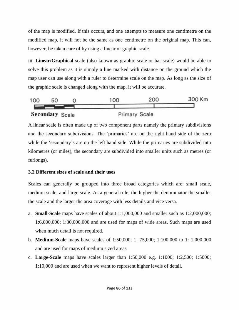
Page 86 of 133

of the map is modified. If this occurs, and one attempts to measure one centimetre on the

modified map, it will not be the same as one centimetre on the original map. This can,

however, be taken care of by using a linear or graphic scale.

iii. Linear/Graphical scale (also known as graphic scale or bar scale) would be able to

solve this problem as it is simply a line marked with distance on the ground which the

map user can use along with a ruler to determine scale on the map. As long as the size of

the graphic scale is changed along with the map, it will be accurate.

A linear scale is often made up of two component parts namely the primary subdivisions

and the secondary subdivisions. The ‘primaries’ are on the right hand side of the zero

while the ‘secondary’s are on the left hand side. While the primaries are subdivided into

kilometres (or miles), the secondary are subdivided into smaller units such as metres (or

furlongs).

3.2 Different sizes of scale and their uses

Scales can generally be grouped into three broad categories which are: small scale,

medium scale, and large scale. As a general rule, the higher the denominator the smaller

the scale and the larger the area coverage with less details and vice versa.

a. Small-Scale maps have scales of about 1:1,000,000 and smaller such as 1:2,000,000;

1:6,000,000; 1:30,000,000 and are used for maps of wide areas. Such maps are used

when much detail is not required.

b. Medium-Scale maps have scales of 1:50,000; 1: 75,000; 1:100,000 to 1: 1,000,000

and are used for maps of medium sized areas

c. Large-Scale maps have scales larger than 1:50,000 e.g. 1:1000; 1:2,500; 1:5000;

1:10,000 and are used when we want to represent higher levels of detail.

Page 87 of 133

It has being stated that a large scale map cover relatively small area but with great detail

,while a small scale map cover large area with less detail. Simply put, a ‘large-scale’

map gives a larger and more detailed representation of a feature than does a ‘small-scale’

map.

3.3 Conversion of scales

In map reading, one can convert from one scale type to another. For instance, we can

convert from statement scale to Representative Fraction (R.F.) and vice versa or from

linear scale to statement or RF, and so on. Examples:

i. Conversion from R.F. to statement scale

Examples:

Convert the following R.F. scales to statement scale:

(a) 1:1000; (b) 1:20,000; (c) 1:150,000

Given that: 100cm =1m; 100,000cm = 1km

Solutions:

For RF of 1:1000, it means 1cm represents 1000cm.

Therefore, the statement scale is 1cm represents 10 metres or 0.01km.

For RF of 1:20,000 it means 1cm represents 20,000cm.

Therefore, the statement scale is 1cm represents 0.2km or 5cm represent 1km.

And for RF of 1:150,000, it means 1cm represents 150,000cm.

Therefore, the statement scale is 1cm represents 1.5km or 2cm represents 3km.

ii. Conversion from statement scale to R.F.

Examples:

Convert the following statement scales to Representative Fraction:

(a) 1cm to ½ km (b) 4cm to 1km

Recall that 1km = 100,000cm

Solutions:

(a) 1cm to ½ km

Page 88 of 133

½km = 100,000 = 50,000cm

Therefore, the R.F. 1:50,000

(b) 4cm to 1km

If 4cm represent 100,000cm,

1cm will represent 100,000 = 25,000cm

Therefore, the R.F 1:25,000

4.0 Conclusion

Scale is one of the vital components of every map and without it, the features represented

cannot be correlated with the actual size on the ground. In fact, any drawing without scale

is not a map. Users of maps must therefore be able to determine the actual ground sizes of

features from any map or translate the map features to the ground for development

purposes.


i. Compare and contrast small and large scale map.

ii. Convert the following statement scales to Representative Fraction:

(a) 1cm to ⅔ km (b) 5cm to 2km

iii. Convert the following R.F. scales to statement scale:

(a) 1:10,000; (b) 1:50,000; (c) 1:250,000


Thomas, I.L., Howarth, F., Eggers, A., and Fowler, A.D.W. (1981). Textural,

Enhancement of a Circular Geologic Feature, Photogrammetric Engineering and

Remote Sensing, 47, pp 89-91.

Page 89 of 133

UNIT 2: MAP CONVENTIONAL SIGNS

CONTENTS

1.0 Introduction

2.0 Objectives

3.0 Main Content

3.1 Natural and man-made features

3.2 Marginal lands symbols

3.3 Informative symbols

4.0 Conclusion



1.0 Introduction

Conventional signs are map symbols that are universally accepted for the representation

of earth features. It is not practically possible to show every bit of detail about any feature

represented on a ground. Hence only those details about each feature which are

considered of outmost important are given on the map. Moreover, one symbol is

normally used to generally represent all features which are considered to be in the same

class or group, irrespective of the individual differences that may exist among the

features grouped together.

2.0 Objectives

The objectives of this unit are as stated below:

To make student acquitted with major map universal symbols

Assist student to be able to read and understand map and image features on maps

Prepare student for group or congress meeting on map related programmes

To help student to be able to deriving meaningful information from maps for

decision support

Page 90 of 133

3.0 Main Content

3.1 Natural and man-made features

Maps naturally contain natural features like hills, ridges, rivers, ditches, erosion features

and man-made (artificial) features like: transport routs, settlements, boundary lines, and

bench marks. The hierarchy of these features and classification is universal in

representation for easy comparison and standardization (see fig. 26).

3.2 Marginal lands symbols

Marginal lands are of different forms and place related, but the concept is the same

globally Marginal lands are localities or land areas where diminishing return has set in.

They are areas of less agricultural productivity or with human developmental difficulty.

Such areas are: badlands, swamps, derelict areas, precipice etc. Such areas are

symbolically represented conventionally for setbacks or conservation (see fig. 26)

3.3 Informative symbols

There are some conventional map symbols that are meant to convey information about

the existence of some facilities, nearness of some service area, like health centre, police

post, post office, mining site, . worship place, historical sites, etc (see figure 26).

Page 91 of 133

Figure 26. Map conventional symbols

Page 92 of 133

Tool symbols

These are conventional symbols that are used to standardize and qualify a map. They are

the symbols that are used to manipulate and analyse the content of the map in relation to

a given locality. These are the Northing directional symbol, the graticules (Lat-Long

lines), the scale, and the legend. This four define a drawing to be a map or not.

4.0 Conclusion

Conventional signs which are map keys or shorthand used by cartographers to avoid the

clumsiness of maps. Map end users must therefore be conversant with those symbols that

are universally accepted to enhance universal usage of maps. In fact, there are

conventional colour codes for some particular natural and artificial earth features like

water bodies, paved roads, contour lines etc.


i. What is the use of map symbols to the Cartographers and map end users.

ii. Which map symbols qualifies a drawing as a map and why

iii. With suitable examples, what are informative symbols


Anji, R.M (2008). Remote Sensing and Geographical Information Systems. Third edition,

BS Publications

Reeves, R.G. (1979). Manual of Remote Sensing, Publisher: Falls Church, Virgina:

American Society of Photogrammetry, ©1975. (OCoLC)624526005

Wise, S. (2018). GIS Basics, Taylor and Francis, London.

DOIhttps://doi.org/10.1201/9781315274768

Page 93 of 133

UNIT 3: IMAGE INTERPRETATION ELEMENTS

CONTENTS

1.0 Introduction

2.0 Objectives

3.0 Main Content

3.1 Types of Imageries

3.2 Interpretation Elements

3.3 Elements combination for interpretation

4.0 Conclusion



1.0 Introduction

Image interpretation is far different from map reading because Aerial photographs and

satellite imageries are photographs taking by different cameral sensors. While maps are

produced by cartographers using conventional symbols that can easily be recognised.

Generally, features on an aerial photograph and satellite imageries are not generalized or

symbolized as in maps as air photos record all visible features on the Earth's surface from

an overhead perspective. Although the features are visible, they are not always easily

identifiable. Skill in image interpretation is acquired over a period of time as experience

gathering. You will therefore be exposed to some of the principles of interpreting

imageries in this unit.

2.0 Objectives


To acquit student with the principles of image interpretation,

Assist student to be able to interpret and understand imagery features

Prepare student for group or congress meeting on image related programmes

Page 94 of 133

To help student to be able to deriving meaningful information from imageries for

decision support

3.0 Main Content

3.1 Types of Imageries

Aerial photographs and satellite imageries are generally grouped according to their

platform and spectral resolutions. Generally, apart from aerial photography that operate at

low or middle altitude, all earth resources satellites operate as polar orbiting satellites

with platforms operated by different countries. For instance, we have Nigeria Sat-X,

Landsat series own by US, Spot series own by France, and many more.

In terms of image spectral resolution, reference is been made to the near clarity of the

feature shown in relation to the ground feature. This can be grouped into two via: Low

and High resolution imageries. Aerial photographs are usually of high resolution as

image 2D features are close to the ground features. The resolution of the air photo/image

actually determine the visual interpretation possibility of the air photo/image, for

instance, Landsat image with 30m resolution is beyond human eye interpretation

adequately. But images from Quick bird, Ikonus and NigeriaSat-X platform with 5m

resolution have a close resemblance of the actual feature on the ground.

3.2 Interpretation Elements

The process of studying and gathering the information required for the identification of

the various cultural and natural features is called photo interpretation. With careful

interpretation, air photos are an excellent source of spatial data for studying the Earth's

environment. Image interpretation is a professional work that requires some experience

most especially when the images are taken in an oblique angle. There are elements that

serve as a guide for the identification and interpretation of spectral signature as discussed

below:

i. Location

The geographical location of an aerial photograph or image helps a lot in

determining the image features and its attributes. When we identify the

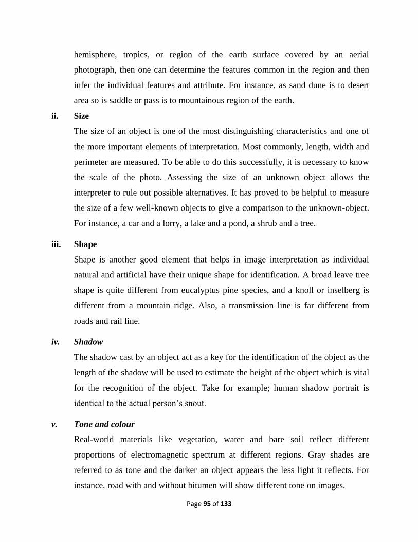
Page 95 of 133

hemisphere, tropics, or region of the earth surface covered by an aerial

photograph, then one can determine the features common in the region and then

infer the individual features and attribute. For instance, as sand dune is to desert

area so is saddle or pass is to mountainous region of the earth.

ii. Size

The size of an object is one of the most distinguishing characteristics and one of

the more important elements of interpretation. Most commonly, length, width and

perimeter are measured. To be able to do this successfully, it is necessary to know

the scale of the photo. Assessing the size of an unknown object allows the

interpreter to rule out possible alternatives. It has proved to be helpful to measure

the size of a few well-known objects to give a comparison to the unknown-object.

For instance, a car and a lorry, a lake and a pond, a shrub and a tree.

iii. Shape

Shape is another good element that helps in image interpretation as individual

natural and artificial have their unique shape for identification. A broad leave tree

shape is quite different from eucalyptus pine species, and a knoll or inselberg is

different from a mountain ridge. Also, a transmission line is far different from

roads and rail line.

iv. Shadow

The shadow cast by an object act as a key for the identification of the object as the

length of the shadow will be used to estimate the height of the object which is vital

for the recognition of the object. Take for example; human shadow portrait is

identical to the actual person’s snout.

v. Tone and colour

Real-world materials like vegetation, water and bare soil reflect different

proportions of electromagnetic spectrum at different regions. Gray shades are

referred to as tone and the darker an object appears the less light it reflects. For

instance, road with and without bitumen will show different tone on images.

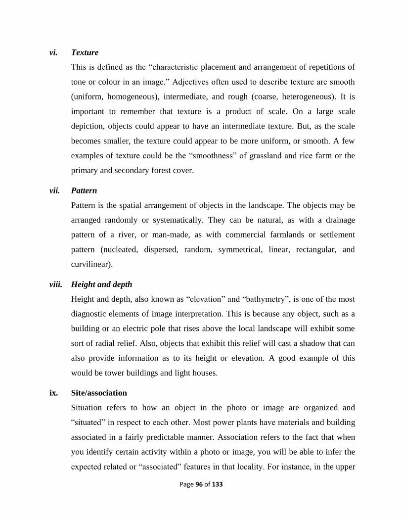
Page 96 of 133

vi. Texture

This is defined as the “characteristic placement and arrangement of repetitions of

tone or colour in an image.” Adjectives often used to describe texture are smooth

(uniform, homogeneous), intermediate, and rough (coarse, heterogeneous). It is

important to remember that texture is a product of scale. On a large scale

depiction, objects could appear to have an intermediate texture. But, as the scale

becomes smaller, the texture could appear to be more uniform, or smooth. A few

examples of texture could be the “smoothness” of grassland and rice farm or the

primary and secondary forest cover.

vii. Pattern

Pattern is the spatial arrangement of objects in the landscape. The objects may be

arranged randomly or systematically. They can be natural, as with a drainage

pattern of a river, or man-made, as with commercial farmlands or settlement

pattern (nucleated, dispersed, random, symmetrical, linear, rectangular, and

curvilinear).

viii. Height and depth

Height and depth, also known as “elevation” and “bathymetry”, is one of the most

diagnostic elements of image interpretation. This is because any object, such as a

building or an electric pole that rises above the local landscape will exhibit some

sort of radial relief. Also, objects that exhibit this relief will cast a shadow that can

also provide information as to its height or elevation. A good example of this

would be tower buildings and light houses.

ix. Site/association

Situation refers to how an object in the photo or image are organized and

“situated” in respect to each other. Most power plants have materials and building

associated in a fairly predictable manner. Association refers to the fact that when

you identify certain activity within a photo or image, you will be able to infer the

expected related or “associated” features in that locality. For instance, in the upper

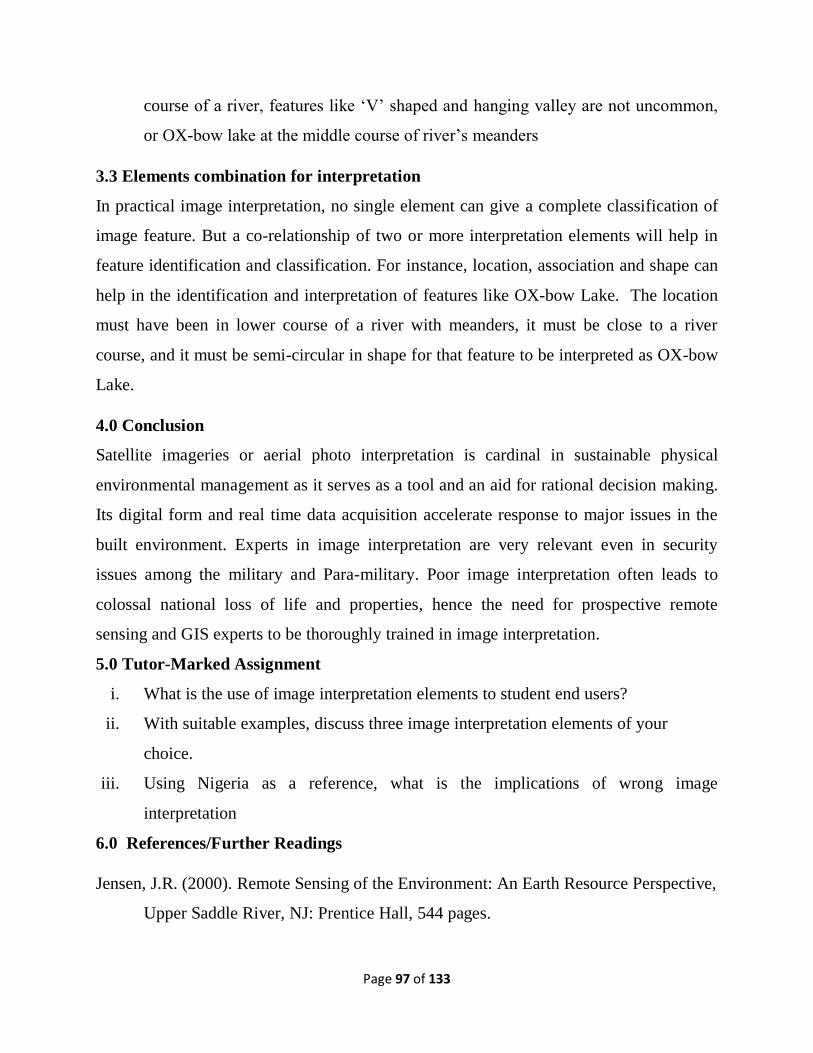
Page 97 of 133

course of a river, features like ‘V’ shaped and hanging valley are not uncommon,

or OX-bow lake at the middle course of river’s meanders

3.3 Elements combination for interpretation

In practical image interpretation, no single element can give a complete classification of

image feature. But a co-relationship of two or more interpretation elements will help in

feature identification and classification. For instance, location, association and shape can

help in the identification and interpretation of features like OX-bow Lake. The location

must have been in lower course of a river with meanders, it must be close to a river

course, and it must be semi-circular in shape for that feature to be interpreted as OX-bow

Lake.

4.0 Conclusion

Satellite imageries or aerial photo interpretation is cardinal in sustainable physical

environmental management as it serves as a tool and an aid for rational decision making.

Its digital form and real time data acquisition accelerate response to major issues in the

built environment. Experts in image interpretation are very relevant even in security

issues among the military and Para-military. Poor image interpretation often leads to

colossal national loss of life and properties, hence the need for prospective remote

sensing and GIS experts to be thoroughly trained in image interpretation.


i. What is the use of image interpretation elements to student end users?

ii. With suitable examples, discuss three image interpretation elements of your

choice.

iii. Using Nigeria as a reference, what is the implications of wrong image

interpretation




Page 98 of 133


Series, 250p.

Reeves, R.G. (1979). Manual of Remote Sensing, Publisher: Falls Church, Virgina:

American Society of Photogrammetry, ©1975. (OCoLC)624526005

Page 99 of 133

UNIT 4: MAP REDUCTION AND ENLARGEMENT

CONTENTS

1.0 Introduction

2.0 Objectives

3.0 Main Content

3.1 Instrumentation and Purpose of map manipulation

3.2 Map Reduction processes

3.3 Map Enlargement processes

4.0 Conclusion



1.0 Introduction

In carrying out environmental studies that require spatial data assemblage especially

analogue Maps of different sources and scales, some of them may require either reduction

or enlargement to meet the present needs. There are series of steps to be followed in

carrying out such activity as discussed below:

2.0 Objectives


i. The student should at the end of this unit, be able to either enlarge or reduce maps

for their own use and also render service to others

ii. To expose student to maps transformation for different uses

iii. Remove the difficulties students often encountered in secondary data integration

and analysis.

Page 100 of 133

3.0 Main Content

3.1 Instrumentation and Purpose of map manipulation

The materials required for map reduction or enlargement are not costly and they are

readily available with us. The format and scale of the map will determine the basic

material usage. Maps in digital form can be manipulated (reduce or enlarged) can be

carried out in GIS laboratory using map enlarger machine. Also an analogue machine

called pantograph can be used also.

Other instruments include:

i. Scale rule

ii. Compass divider

iii. Straight edge (ruler)

iv. Calculator

3.2 Map Reduction processes

The process of map reduction is quite simple where there are hand-on practices. The

following steps should be followed sequentially to get this done.

i. Measure the length and width of the map

ii. To reduce the map to half of its original size, divide the length and width by 2 For

example, if the length and width of a map are 24cm and 20cm respectively, then the new

dimensions will now be such a map should measure 12cm by 10cm.

iii. The reduction has affect the scale, therefore, if the original map scale is 1:50,000, the

new scale will changes to 1:100,000

iv. The features to be shown on the reduced map should also be proportional to the

required size of the map.

v. When these are accomplished, the title and the new horizontal scale should be

indicated.

Page 101 of 133

3.3 Map Enlargement processes

The process of map enlargement is also simple as the reduction where there are hand-on

practices. The following steps also should be followed sequentially to get this done.

i. Measure the length and width of the original map.

ii. To enlarge twice the original size, multiply the length and width by 2. For example, if

the length and width of a map are 7cm and 5cm respectively, such a map would measure

14cm by 10cm

iii. The enlargement has also affected the original map scale, Therefore, if the map scale

is 1:50,000, the scale of the map changes to 1:25,000

iv. The features to be drawn on the enlarged map should also be proportional to the size

of the map.

v. When these are fully accomplished, the title and the new horizontal scale should be

indicated.

Before one can know whether to reduce or enlarge a map, it may be necessary to divide

the initial scale (scale of the original map) by the scale of the new map to be drawn. For

example, if the scale of a map is 1:50,000 and is to be reproduced to a scale of 1:200,000,

divide the former scale with the latter (50000/200000=1/4). The new map should be 1/4

times the size of the original map.

4.0 Conclusion

Maps are produced for different purposes, and this influences the scale at a point in time.

Ability to either reduce or enlarge maps will go a long way in removing the pain and cost

of having to be looking for map vendors to buy new maps for different projects where the

existing one will suffice. It is therefore expected of every map users to have some skill in

map manipulation to meet different uses except otherwise demand.


i. With examples, how can one determine the number of times a map is either

reduced or enlarged

Page 102 of 133

ii. Using the map given on scale 1: 50,000, reduce the map five times its size, and

give the implication on the features resolution.

iii. Using the map given on scale 1:250,000, enlarge the map four times its size, and

give the implications on the features resolution.

Page 103 of 133

UNIT 5: MAP DIGITIZATION (On-screen and Tablet)

CONTENTS

1.0 Introduction

2.0 Objectives

3.0 Main Content

3.1 General operation of digitizers

3.2 Manual digitization

3.3 On-screen digitization

3.4 Problems of map Digitization

4.0 Conclusion



1.0 Introduction

Analogue data are normally in paper form and include paper maps, tables of statistics and

hardcopy aerial photographs. All these forms of data need to be converted to digital form

before use in a GIS. Digital data like remote sensing data are already in computer

readable formats are supplied on CD-ROM or across a computer network. All data in

analogue form need to be converted to digital form before they can be input into digital

analysis. There are four methods of data input which are widely used: keyboard entry,

manual digitising, automatic digitisation, and scanning. Digital data must be downloaded

from their source media and may require reformatting to convert them to an appropriate

format for the computer being used. Reformatting or conversion may also be required

after analogue data have been converted to digital form. For example, after scanning a

paper map, the file produced by the scanning equipment may not be compatible with the

software, so it needs reformatting.

Page 104 of 133

2.0 Objectives

The objectives of this unit are as listed below:

i. At the end of this study unit, student should be able to understand and the

usefulness of digitizers in spatial data analysis.

ii. The student should be able to differentiate between manual and computer aided

digitization.

iii. Student should be able to give operational steps for tablet and on-screen

digitization.

iv. Acquit students with Problems associated with map Digitization generally.

3.0 Main Content

3.1 General operation of digitizers

Digitisers are the most common device for extracting spatial information from maps and

photographs. The position of an indicator as it is moved over the surface of the digitising

tablet is detected by the computer and interpreted as pairs of x, y coordinates. The

indicator may be a pen-like stylus or a cursor. Frequently, there are control buttons on the

cursor which permit control of the system without having to turn attention from the

digitising tablet to a computer terminal. The current most popular digitiser is

contemporary tablets using a gird of wires embedded in the tablet to a generate magnetic

field which is detected by the cursor. The accuracy of such tables are typically better than

0.1 mm which is better than the accuracy with which the average operator can position

the cursor. Sometimes the functions for transforming coordinates are built into the tablet

and used to process data before it is sent to the host (see figure 27).

3.2 Manual digitization

Manual digitising is the most common method of encoding spatial features from paper

maps. It is a process of converting the spatial features on a map into a digital format.

Point, line, and area features that form a map, are converted into (x, y) coordinates. A

point is represented by a single coordinate, a line by a string of coordinates, and, when

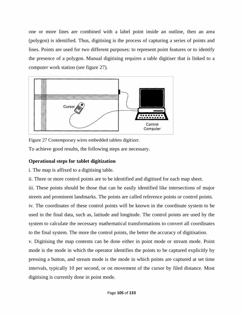
Page 105 of 133

one or more lines are combined with a label point inside an outline, then an area

(polygon) is identified. Thus, digitising is the process of capturing a series of points and

lines. Points are used for two different purposes: to represent point features or to identify

the presence of a polygon. Manual digitising requires a table digitiser that is linked to a

computer work station (see figure 27).

Figure 27 Contemporary wires embedded tablets digitizer.

To achieve good results, the following steps are necessary.

Operational steps for tablet digitization

i. The map is affixed to a digitising table.

ii. Three or more control points are to be identified and digitised for each map sheet.

iii. These points should be those that can be easily identified like intersections of major

streets and prominent landmarks. The points are called reference points or control points.

iv. The coordinates of these control points will be known in the coordinate system to be

used in the final data, such as, latitude and longitude. The control points are used by the

system to calculate the necessary mathematical transformations to convert all coordinates

to the final system. The more the control points, the better the accuracy of digitisation.

v. Digitising the map contents can be done either in point mode or stream mode. Point

mode is the mode in which the operator identifies the points to be captured explicitly by

pressing a button, and stream mode is the mode in which points are captured at set time

intervals, typically 10 per second, or on movement of the cursor by filed distance. Most

digitising is currently done in point mode.

Page 106 of 133

3.3 On-screen digitization

On-screen digitization is carried out by professionals in GIS where image data are

already in digital form or in other format different from GIS environment but need

theme-by-theme map production. For instance, a theme focus may be on transport routs,

marginal lands, encroachment areas, etc. The steps are as discussed below:

i. Import the map into the GIS environment in the appropriate software,

ii. Open the imported file in right GIS software,

iii. There may be need to carryout image enhancement to bring the map feature of interest

to the foreground

iv. Select the digitization menu from the screen dashboard,

v. With the use of the mouse, click along the features to be digitized to the end, and then

double click to end a segment.

vi. Continue the process until all the features of interest are covered,

vii. Depending on the feature of interest, which may be line, point, or polygonal, and the

hierarchy among the features will determine the colouration on the new map so produced.

viii. Develop the map legend including the north direction and scale using the appropriate

menu on the screen dashboard.

ix. Export the new map to where it is needed save or print out copies.

3.4 Problems of map Digitization

The problems that come during the process of converting the maps into digital mode

through the process of digitization vary from one CAD operator to another. It depends

upon the experience and skill of the operator and density of points, lines and polygons of

the map. The accuracy of the output of the digitization also depends upon the selection

and distribution of the control points. Some of the commonly occurred problems during

the digitization of any paper map are as follows:

i. Paper maps are unstable; each time the map is removed from the digitising table,

the reference points must be re-entered when the map is affixed to the table again.

Page 107 of 133

ii. If the map has stretched or shrunk in the interim, the newly digitised points will be

slightly off in their location when compared to previously digitised points.

iii. Errors occur on these maps, and these errors are entered into the GIS data base as

well.

iv. The level of error in the GIS database is directly related to the error level of the

source maps.

v. Maps are meant to display information, and do not always accurately record

vocational information.

4.0 Conclusion

Map or image digitization is an important aspect of digital spatial data management and

GIS activities. Analogue inputs can therefore be converted into digital format through

digitization processes. Also, air photo/image analysis and interpretation often contain

multivariate information that theme-by-theme analysis will require the digitization of the

features of the theme in term of area or lineaments to produce another new thematic map.


i. What are the major differences between table and on-screen digitization, and also

list three of their associated problems.

ii. Using the aerial photo given, digitize all the major road networks to create an

updated township road network.

iii. Discuss fully the major challenges facing manual map digitization and give the way

forward.


Chrisman, N.R. (1978). “Effi cient Digitizing through the Combination of Appropriate

Hardware and Software for Error Detection and Editing,” International Journal of

Geographical Information Systems 1:265–77.

Anji, R.M (2008). Remote Sensing and Geographical Information Systems. Third edition,

BS Publications


Page 108 of 133

MODULE FOUR

ELEMENT OF CARTOGRAPHY

Unit 1: History of maps

Unit 2: Map classification and symbols

Unit 3 Basic form-lines, contouring and cross-sections

Unit 4: Map orientation and layouts

UNIT 1: HISTORY OF MAPS

CONTENTS

1.0 Introduction

2.0 Objectives

3.0 Main Content

3.1 The pre-Roman Empire cartographers

3.2 The post-Roman Empire cartographers

3.3 Ordnance Survey Developments

3.4 Using and Learning Maps

3.5 Roles of Maps

4.0 Conclusion



1.0 Introduction

Map production is as old as human settlements and civilization that is dated back as far as

1292 B.C. Maps are been used for political reasons and territorial command for tribute

collection and kingdom expansion. A clear understanding of the history of map

production and usage by modern day generation and by extension the student will go a

long way to reveal the importance of map for spatial environmental management and

Page 109 of 133

technological trends that metamorphosis to the present day digitally based maps and their

multidisciplinary usage.

As the saying goes that ‘a proper understanding of the past will reveal the base of the

present condition of things, which will in turn helps to project into the future’ This unit

will therefore discuss fully the historical background of map production, various types of

maps, areas of applications, and the general importance of maps to all human generation.

2.0 Objectives

The objective of this unit therefore is to:

i. Help student to understand and appreciate the labour of the Ptolemaeus’s

Geographers and historians in developing the foundation of the present day

modern maps.

ii. Understand the trends and the processes of map production metamorphoses and

applications.

iii. Understand the true definition and use of maps as against the layman knowledge.

iv. Understand the role of maps in general human society.

3.0 Main Content

3.1 The pre-Roman Empire cartographers

The earliest known maps were drawn on parchment to show the gold mines at Coptes

during the reign (1292 – 1225 B.C.) of Rameses II of Egypt. Perhaps earlier still are

Babylonian cuneiform tablets that describe the world as it was then known. At a later

date, the Greeks acquired cartographic skills and compiled the first realistic maps. They

began using a rectangular coordinate system for making maps around 300 B.C. About

100 years later, the Greek mathematician, astronomer, and geographer Eratosthenes (ca.

276 – 194 B.C.) laid the foundations of scientific cartography. One of the earliest known

maps of the world was constructed by Claudius Ptolemaeus of Alexandria (ca. A.D. 90 –

168).

Page 110 of 133

The Romans were more concerned with tabulations and registers. The terms cadastre (an

official property register) and cadastral (of a map or survey that shows property or other

boundaries) originate from the Late Greek kattá-stíkon, which means ‘by line’. But it was

the Romans who first employed the concept to record properties, in the capitum registra,

literally, ‘land register’. In many countries, the term cadastre designates map and

property registers. Throughout history, as societies organized, it became necessary to

meet the expense of this. Some of the better known earlier examples include taxation

levied by emperors and kings to meet military expenses. These direct levies are the

foundations of today’s complicated revenue systems involving the taxation of income,

property, and goods. Since both the ancient Egyptians and the Romans taxed property,

property registration was early systematized to assure tax revenues.

3.2 The post-Roman Empire cartographers

The earliest maps were drawn almost exclusively to facilitate commercial sea voyages.

On them, coasts were meticulously detailed and harbours were plumbed, while interiors

remained unknown, apart from details of important trade and caravan routes. The Arabs

were the leading cartographers of the Middle Ages. European cartography degenerated as

the Roman Empire fell. But in the fifteenth century, old skills were revived and Claudius

Ptolemaeus’s Geographia was translated into Latin to become the then existent view of

the world (see figure 35). Although cartography was neglected, in many countries

property registry thrived. The best known example is the Domesday Book, the record of

the lands of England compiled in 1086 for the first Norman king, William the Conqueror

(1027–87). The data included specifications of properties and their value, and a count of

inhabitants and livestock, as well as incomes earned and taxes paid.

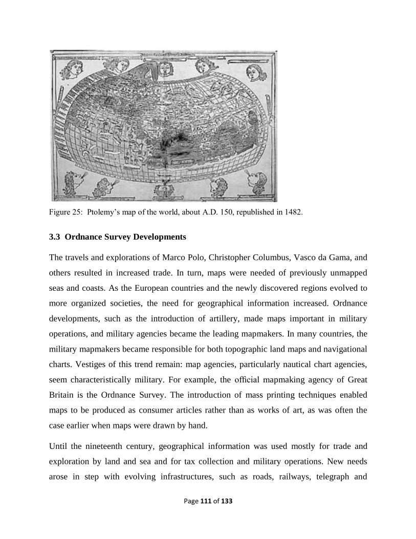
Page 111 of 133

Figure 25: Ptolemy’s map of the world, about A.D. 150, republished in 1482.

3.3 Ordnance Survey Developments

The travels and explorations of Marco Polo, Christopher Columbus, Vasco da Gama, and

others resulted in increased trade. In turn, maps were needed of previously unmapped

seas and coasts. As the European countries and the newly discovered regions evolved to

more organized societies, the need for geographical information increased. Ordnance

developments, such as the introduction of artillery, made maps important in military

operations, and military agencies became the leading mapmakers. In many countries, the

military mapmakers became responsible for both topographic land maps and navigational

charts. Vestiges of this trend remain: map agencies, particularly nautical chart agencies,

seem characteristically military. For example, the official mapmaking agency of Great

Britain is the Ordnance Survey. The introduction of mass printing techniques enabled

maps to be produced as consumer articles rather than as works of art, as was often the

case earlier when maps were drawn by hand.

Until the nineteenth century, geographical information was used mostly for trade and

exploration by land and sea and for tax collection and military operations. New needs

arose in step with evolving infrastructures, such as roads, railways, telegraph and

Page 112 of 133

telephone lines, and gas and water supplies. Planning these facilities required information

about the terrain beyond that commonly available. The accurate location of towns and

cities, lakes and rivers, mountains and valleys became increasingly important. Detailed

topographic information was needed to layout railway and road gradients and curve radii.

Then, as now, foundations were a major challenge, so maps showing the type of soil and

the quality, location, and properties of bedrock were required. As planning advanced,

specialized maps became more common. The first geological map of Paris was compiled

in 1811. In 1838, the Irish government compiled a series of maps for the use of railway

engineers, which may be regarded as the first manual geographical information system.

As cities grew larger and more complex, accurate urban planning became a necessity.

Many countries began compiling statistical information relating to urban planning in the

early nineteenth century. By 1837 the British Registrar General’s Office had amassed

extensive population statistics. Traditional village property ownership became a

hindrance to effective farming. Many properties had become fragmented over the years,

owing to inheritance settlements. In some cases a single property might comprise several

hundred dispersed parcels of land. Sometimes the ownership of, or rights to a parcel were

divided: one owner could have timber rights, another grazing right, and so on. Therefore,

property mapping in the late nineteenth century aimed to wrest order from chaos. With

reference to available land registers, the various parcels were assembled into properties

that were easier to work. Borders were consolidated, clarifying ownership and facilitating

the taxation of property.

Aerial photography accelerated the progress of mapmaking. The first aerial photograph

was used for mapmaking, and the first mapmaking instrument devised, in 1909.

Photogrammetry, the technique of making measurements from photographs, developed

rapidly in the 1920s and 1930s, and the two world wars also hastened developments.

After World War II, photogrammetry became widely used in mapmaking, mostly for

maps in scales from 1:500 to 1:50,000. Aerial photographs themselves became important

Page 113 of 133

sources of quantitative information in evaluating such features as vegetation and

geological formation.

3.4 Using and Learning Maps

By definition, according to the International Cartographic Association, a map is a

representation, normally to scale and on a flat medium, of a selection of material or

abstract features on, or in relation to, the surface of the Earth. The term ‘map’ is often

used in mathematics to convey the notion of transferring information from one form to

another, just as cartographers transfer information from the surface of the Earth to a sheet

of paper. The term ‘map’ is used loosely to refer to any visual display of information,

particularly if it is abstract, generalized or schematic. Cartography is very much a process

of abstraction in which features of the real world are generalized or simplified to meet the

demands of the theme and audience. Not all elements or details have a bearing on the

pattern or process being studied and so some are eliminated to draw the reader’s attention

to those facts that are relevant. Too much detail can even hide or disguise the message of

a map. The amount of detail that can be included is very much dependent on the scale at

which the map will be produced, as the following examples demonstrate. A small-scale

map of an area must, almost of necessity, be more generalized.

The term Cartography comes from two Greek words, chartis, meaning map, and graphos,

meaning to draw or write. In historic times, an individual cartographer will hand draw a

map in its entirety, often with limited information The main purpose of cartographic

maps is to communicate geographical information and support geographical problem-

solving. Humans have the ability to quickly extract great amounts of information from

spatial depictions (images) like pictures or graphs. Even non-spatial or non-perceivable

information can be displayed this way (visualization or specialization). Maps use

convenient scales and viewing perspectives (we can perceive all from a single

viewpoint). Maps highlight and clarify relevant properties; omit or downplay irrelevant

properties. But projections, generalizations, exaggerations, omissions may mislead or

distort knowledge in a map. Similarly, perspective translation from overhead to terrain-

Page 114 of 133

level view may be confusing or interpretation of symbols (colours, point symbols,

contour lines) may be difficult or misleading. However, training and experience with

maps changes the way they are perceived and interpreted.

Map is a representation, normally to scale and on a flat medium, of a selection of material

or abstract features on, or in relation to, the surface of the Earth. Production of a map

requires: selection of the few features in the real world to include, classification of

selected features into groups (i.e., bridges, houses, railways), simplification of jagged

lines like coastlines, exaggeration of features to be included that are too small to show at

the scale of the map and symbolization to represent the different classes of features

chosen.

3.5 Roles of Maps

Traditionally, maps have four roles as listed below:

a. Data display-maps provide useful ways of displaying information in a meaningful

way.

b. Data storage - as a means of storing data.

c. Spatial indexes - a map can show the boundaries of areas (e.g., land use zones, soil or

rock

types) and identify each area with a label.

d. Data analysis tool - maps are used in analysis to make or test hypotheses and

examine the

relationship between two distributions using simple transparent overlays.

Computer Cartography

Computer cartography has a primary goal of producing maps, systems have advanced

tools for map layout, placement of labels, large symbol and font libraries, interfaces for

expensive, high quality output devices. However, it is not an analytical tool, therefore,

unlike data for GIS, cartographic data does not need to be stored in ways which allow, for

Page 115 of 133

example, analysis of relationships between different themes such as population density

and housing prices or the routing of flows along connecting highway or river segments.

4.0 Conclusion

Map production and usage has passed through series changes over the years. There is also

a great transformation in the operation cartographic activities to the present day computer

based cartography. The use and application of map products has also being widening as

technology increases. Environmental management student therefore have much to grasp

to be able to address the continuous and dynamic natural and man-induced land use

challenges.


i. Discuss in detail the Ptolemaeus’s map production and usage.

ii. Compare and contrast the computer cartography and ordinance survey.

iii. What are the major roles of maps in the present day human development.


Clarke, K.C. (1990). Analytical and Computer Cartography. Prentice-Hall, Englewood

Cliffs, New Jersey.

Densham, P.J., and Rushton, G. (1988). Decision Support Systems for Locational

Planning, in R. Golledge and H. Timmermans, editors, Behavioural Modelling in

Geography and Planning. Croom-Helm, London, pp. 56–90.

Aronoff, S. (1989). Geographic Information Systems: A Management Perspective. WDL

Publications, Ottawa.

Berry, B.J.L., and Baker, A.M. (1968). Geographic sampling. In B.J.L. Berry and D.F.

Marble, editors, Spatial Analysis. Prentice Hall, Englewood Cliffs NJ, 91–100.

Berry, J.K. (1987). Fundamental Operations in Computer– assisted Map Analysis,

International Journal of Geographical Information Systems 1:119–136.

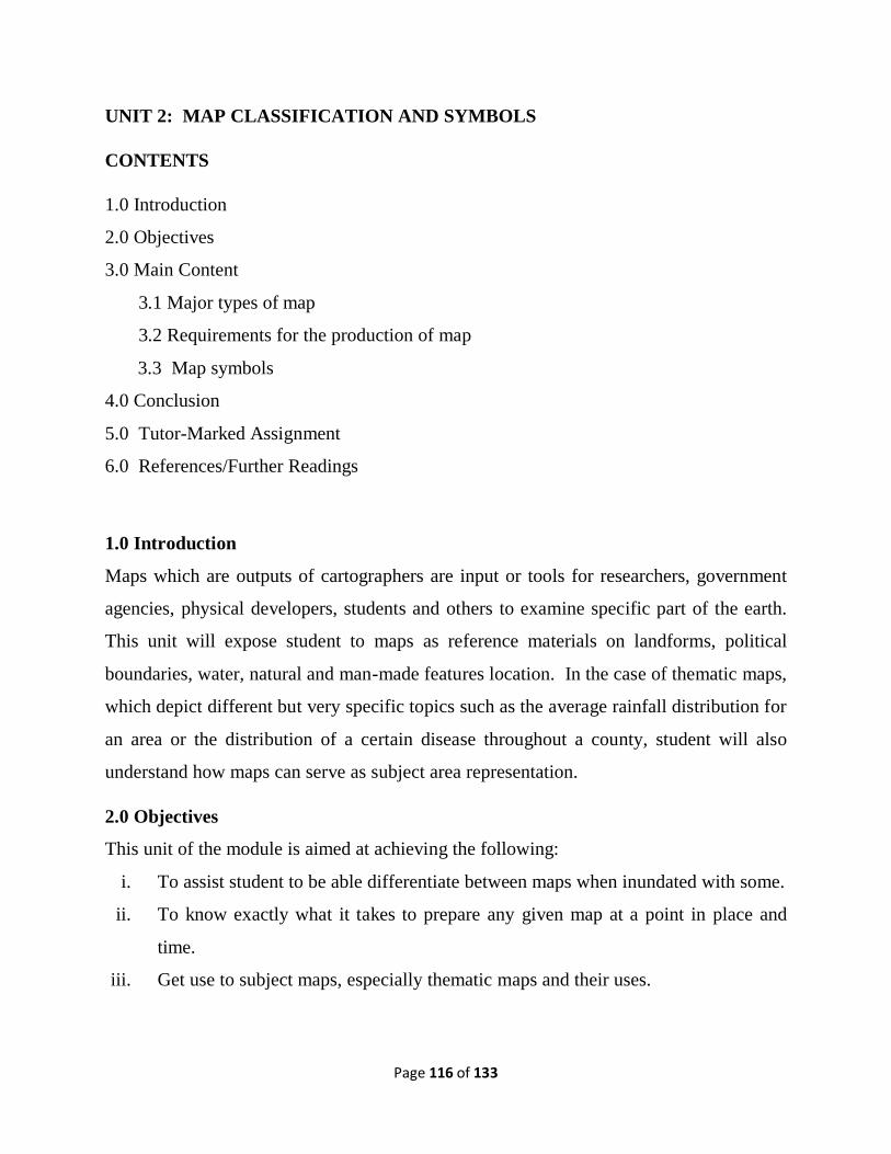
Page 116 of 133

UNIT 2: MAP CLASSIFICATION AND SYMBOLS

CONTENTS

1.0 Introduction

2.0 Objectives

3.0 Main Content

3.1 Major types of map

3.2 Requirements for the production of map

3.3 Map symbols

4.0 Conclusion



1.0 Introduction

Maps which are outputs of cartographers are input or tools for researchers, government

agencies, physical developers, students and others to examine specific part of the earth.

This unit will expose student to maps as reference materials on landforms, political

boundaries, water, natural and man-made features location. In the case of thematic maps,

which depict different but very specific topics such as the average rainfall distribution for

an area or the distribution of a certain disease throughout a county, student will also

understand how maps can serve as subject area representation.

2.0 Objectives

This unit of the module is aimed at achieving the following:

i. To assist student to be able differentiate between maps when inundated with some.

ii. To know exactly what it takes to prepare any given map at a point in place and

time.

iii. Get use to subject maps, especially thematic maps and their uses.

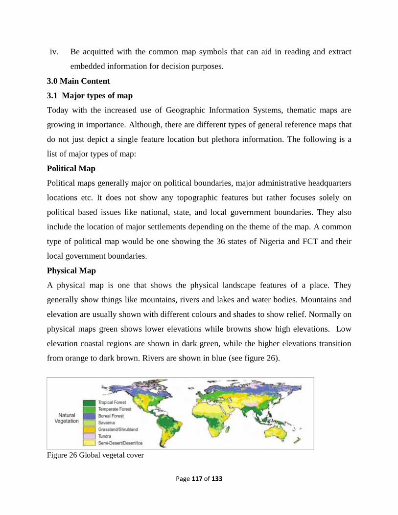
Page 117 of 133

iv. Be acquitted with the common map symbols that can aid in reading and extract

embedded information for decision purposes.

3.0 Main Content

3.1 Major types of map

Today with the increased use of Geographic Information Systems, thematic maps are

growing in importance. Although, there are different types of general reference maps that

do not just depict a single feature location but plethora information. The following is a

list of major types of map:

Political Map

Political maps generally major on political boundaries, major administrative headquarters

locations etc. It does not show any topographic features but rather focuses solely on

political based issues like national, state, and local government boundaries. They also

include the location of major settlements depending on the theme of the map. A common

type of political map would be one showing the 36 states of Nigeria and FCT and their

local government boundaries.

Physical Map

A physical map is one that shows the physical landscape features of a place. They

generally show things like mountains, rivers and lakes and water bodies. Mountains and

elevation are usually shown with different colours and shades to show relief. Normally on

physical maps green shows lower elevations while browns show high elevations. Low

elevation coastal regions are shown in dark green, while the higher elevations transition

from orange to dark brown. Rivers are shown in blue (see figure 26).

Figure 26 Global vegetal cover

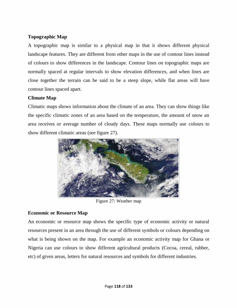
Page 118 of 133

Topographic Map

A topographic map is similar to a physical map in that it shows different physical

landscape features. They are different from other maps in the use of contour lines instead

of colours to show differences in the landscape. Contour lines on topographic maps are

normally spaced at regular intervals to show elevation differences, and when lines are

close together the terrain can be said to be a steep slope, while flat areas will have

contour lines spaced apart.

Climate Map

Climatic maps shows information about the climate of an area. They can show things like

the specific climatic zones of an area based on the temperature, the amount of snow an

area receives or average number of cloudy days. These maps normally use colours to

show different climatic areas (see figure 27).

Figure 27: Weather map

Economic or Resource Map

An economic or resource map shows the specific type of economic activity or natural

resources present in an area through the use of different symbols or colours depending on

what is being shown on the map. For example an economic activity map for Ghana or

Nigeria can use colours to show different agricultural products (Cocoa, cereal, rubber,

etc) of given areas, letters for natural resources and symbols for different industries.

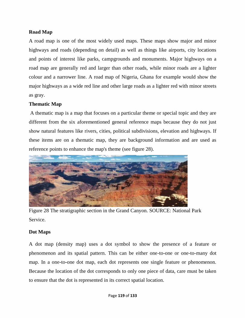
Page 119 of 133

Road Map

A road map is one of the most widely used maps. These maps show major and minor

highways and roads (depending on detail) as well as things like airports, city locations

and points of interest like parks, campgrounds and monuments. Major highways on a

road map are generally red and larger than other roads, while minor roads are a lighter

colour and a narrower line. A road map of Nigeria, Ghana for example would show the

major highways as a wide red line and other large roads as a lighter red with minor streets

as gray.

Thematic Map

A thematic map is a map that focuses on a particular theme or special topic and they are

different from the six aforementioned general reference maps because they do not just

show natural features like rivers, cities, political subdivisions, elevation and highways. If

these items are on a thematic map, they are background information and are used as

reference points to enhance the map's theme (see figure 28).

Figure 28 The stratigraphic section in the Grand Canyon. SOURCE: National Park

Service.

Dot Maps

A dot map (density map) uses a dot symbol to show the presence of a feature or

phenomenon and its spatial pattern. This can be either one-to-one or one-to-many dot

map. In a one-to-one dot map, each dot represents one single feature or phenomenon.

Because the location of the dot corresponds to only one piece of data, care must be taken

to ensure that the dot is represented in its correct spatial location.

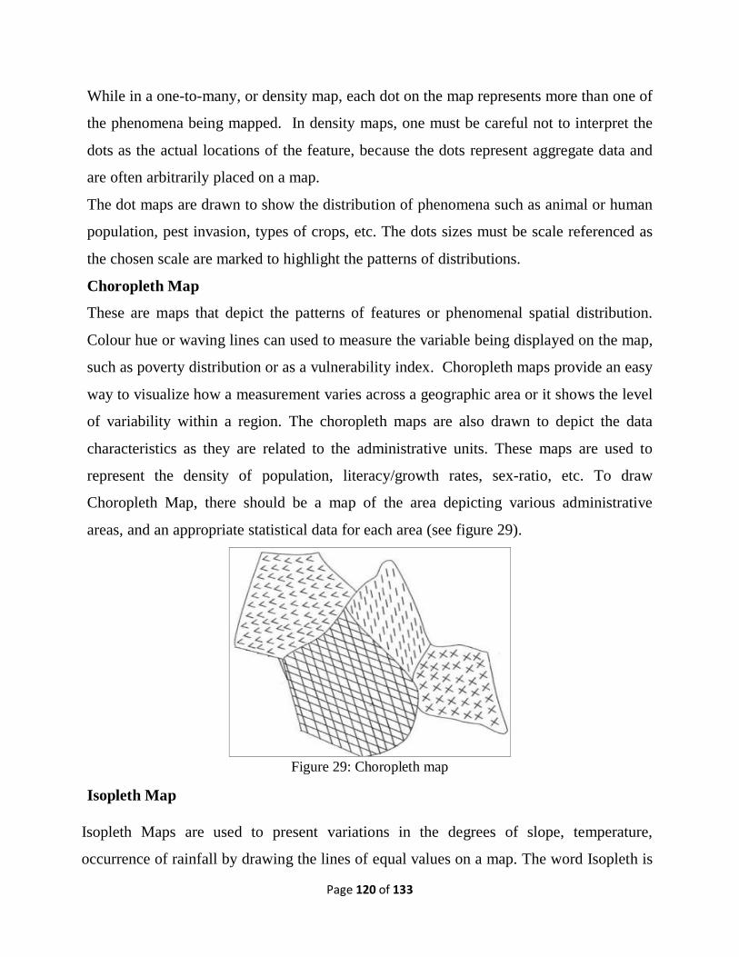
Page 120 of 133

While in a one-to-many, or density map, each dot on the map represents more than one of

the phenomena being mapped. In density maps, one must be careful not to interpret the

dots as the actual locations of the feature, because the dots represent aggregate data and

are often arbitrarily placed on a map.

The dot maps are drawn to show the distribution of phenomena such as animal or human

population, pest invasion, types of crops, etc. The dots sizes must be scale referenced as

the chosen scale are marked to highlight the patterns of distributions.

Choropleth Map

These are maps that depict the patterns of features or phenomenal spatial distribution.

Colour hue or waving lines can used to measure the variable being displayed on the map,

such as poverty distribution or as a vulnerability index. Choropleth maps provide an easy

way to visualize how a measurement varies across a geographic area or it shows the level

of variability within a region. The choropleth maps are also drawn to depict the data

characteristics as they are related to the administrative units. These maps are used to

represent the density of population, literacy/growth rates, sex-ratio, etc. To draw

Choropleth Map, there should be a map of the area depicting various administrative

areas, and an appropriate statistical data for each area (see figure 29).

Figure 29: Choropleth map

Isopleth Map

Isopleth Maps are used to present variations in the degrees of slope, temperature,

occurrence of rainfall by drawing the lines of equal values on a map. The word Isopleth is

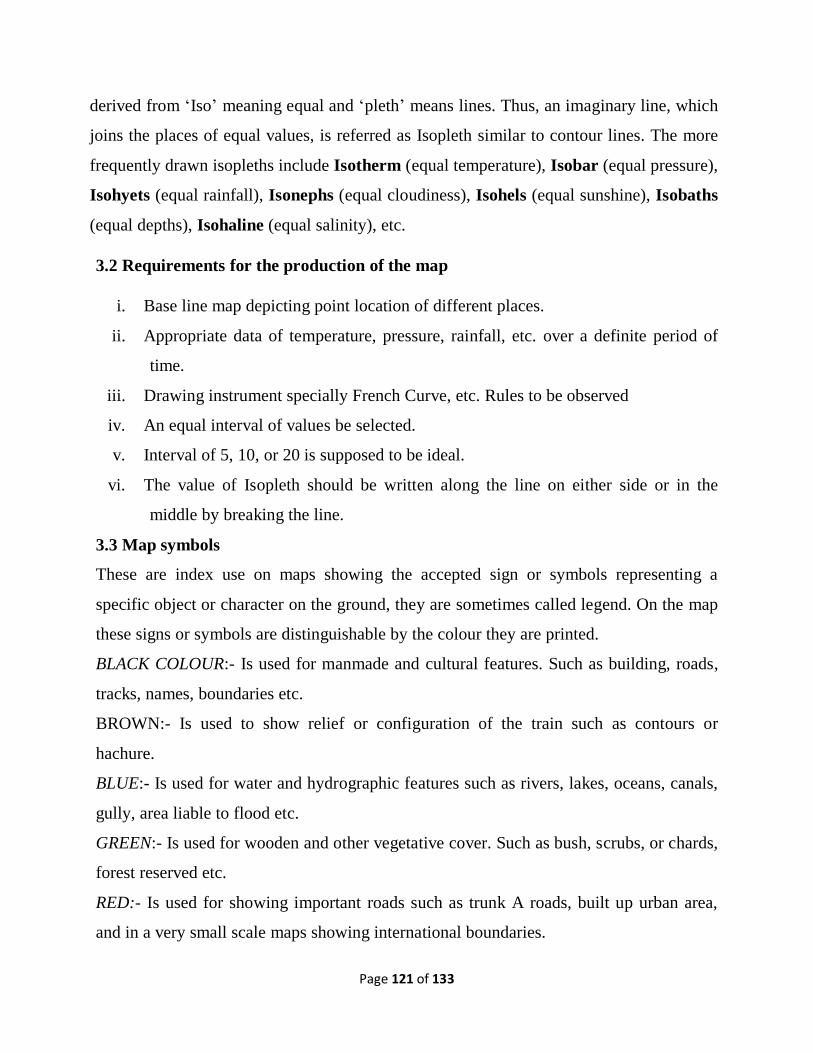
Page 121 of 133

derived from ‘Iso’ meaning equal and ‘pleth’ means lines. Thus, an imaginary line, which

joins the places of equal values, is referred as Isopleth similar to contour lines. The more

frequently drawn isopleths include Isotherm (equal temperature), Isobar (equal pressure),

Isohyets (equal rainfall), Isonephs (equal cloudiness), Isohels (equal sunshine), Isobaths

(equal depths), Isohaline (equal salinity), etc.

3.2 Requirements for the production of the map

i. Base line map depicting point location of different places.

ii. Appropriate data of temperature, pressure, rainfall, etc. over a definite period of

time.

iii. Drawing instrument specially French Curve, etc. Rules to be observed

iv. An equal interval of values be selected.

v. Interval of 5, 10, or 20 is supposed to be ideal.

vi. The value of Isopleth should be written along the line on either side or in the

middle by breaking the line.

3.3 Map symbols

These are index use on maps showing the accepted sign or symbols representing a

specific object or character on the ground, they are sometimes called legend. On the map

these signs or symbols are distinguishable by the colour they are printed.

BLACK COLOUR:- Is used for manmade and cultural features. Such as building, roads,

tracks, names, boundaries etc.

BROWN:- Is used to show relief or configuration of the train such as contours or

hachure.

BLUE:- Is used for water and hydrographic features such as rivers, lakes, oceans, canals,

gully, area liable to flood etc.

GREEN:- Is used for wooden and other vegetative cover. Such as bush, scrubs, or chards,

forest reserved etc.

RED:- Is used for showing important roads such as trunk A roads, built up urban area,

and in a very small scale maps showing international boundaries.

Page 122 of 133

There are conventional signs (symbols) as discussed earlier in the previous modules,

some of them are repeated below:

Figure 30. Map symbols

4.0 Conclusion

There are different types of map with single or multipurpose uses. An environmental

manager should be able to recognize and classify maps ease as discussed above. Each

map is produced for specific purposes with keys or symbols for interpretation. The

discussion above has elucidated and reveals to the student various maps that can acquire

or produced for different project. All this will help in the final examination and after

academic life.


i. Write short not on the following (Chloroplet maps, Isoyet map, Political maps,

Isoplet map, and Dot map).

ii. With suitable examples, Differentiate between Thematic and Topographic maps.

iii. What is map symbol, list and explain five of them with illustrations.


Kemp, K.K., and Goodchild, M.F. (1991). Developing a Curriculum in Geographic

Information Systems: The National Center for Geographic Information and

Analysis Core Curriculum Project. Journal of Geography in Higher Education,

vol. 15, no.2, pp. 121–132.

Lillesand, T.M., and Kiefer, R.W. (2004). “Remote Sensing and Image Interpretation”,

Page 123 of 133

5th Edition, John Wiley & Sons.

Peterson, M.P. (1995). Interactive and Animated Cartography. Upper Saddle River, NJ:

Prentice Hall.

Peuquet, D.J. (1981). An Examination of Techniques for Reformatting Digital

Cartographic Data, Part II: The Vector-to-raster Process, Cartographica 18:21–33.

Peuquet, D.J. (1991). Methods for Structuring Digital Cartographic Data in a Personal

Computer Environment. In Geographic Information Systems: The Microcomputer

and Modern Cartography by Taylor, D.R.F. (ed.), Pergamon Press, Oxford.

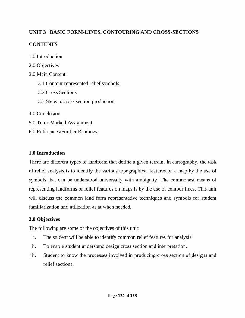
Page 124 of 133

UNIT 3 BASIC FORM-LINES, CONTOURING AND CROSS-SECTIONS

CONTENTS

1.0 Introduction

2.0 Objectives

3.0 Main Content

3.1 Contour represented relief symbols

3.2 Cross Sections

3.3 Steps to cross section production

4.0 Conclusion



1.0 Introduction

There are different types of landform that define a given terrain. In cartography, the task

of relief analysis is to identify the various topographical features on a map by the use of

symbols that can be understood universally with ambiguity. The commonest means of

representing landforms or relief features on maps is by the use of contour lines. This unit

will discuss the common land form representative techniques and symbols for student

familiarization and utilization as at when needed.

2.0 Objectives

The following are some of the objectives of this unit:

i. The student will be able to identify common relief features for analysis

ii. To enable student understand design cross section and interpretation.

iii. Student to know the processes involved in producing cross section of designs and

relief sections.

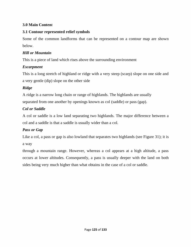
Page 125 of 133

3.0 Main Content

3.1 Contour represented relief symbols

Some of the common landforms that can be represented on a contour map are shown

below.

Hill or Mountain

This is a piece of land which rises above the surrounding environment

Escarpment

This is a long stretch of highland or ridge with a very steep (scarp) slope on one side and

a very gentle (dip) slope on the other side

Ridge

A ridge is a narrow long chain or range of highlands. The highlands are usually

separated from one another by openings known as col (saddle) or pass (gap).

Col or Saddle

A col or saddle is a low land separating two highlands. The major difference between a

col and a saddle is that a saddle is usually wider than a col.

Pass or Gap

Like a col, a pass or gap is also lowland that separates two highlands (see Figure 31); it is

a way

through a mountain range. However, whereas a col appears at a high altitude, a pass

occurs at lower altitudes. Consequently, a pass is usually deeper with the land on both

sides being very much higher than what obtains in the case of a col or saddle.

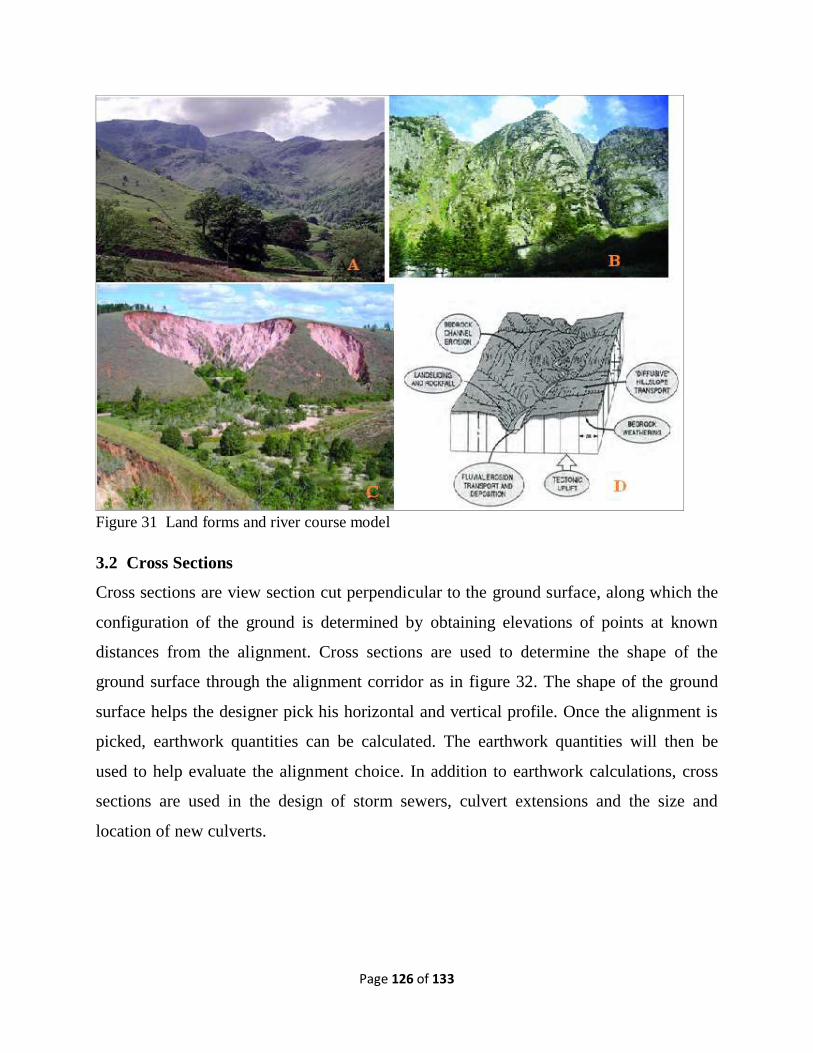
Page 126 of 133

Figure 31 Land forms and river course model

3.2 Cross Sections

Cross sections are view section cut perpendicular to the ground surface, along which the

configuration of the ground is determined by obtaining elevations of points at known

distances from the alignment. Cross sections are used to determine the shape of the

ground surface through the alignment corridor as in figure 32. The shape of the ground

surface helps the designer pick his horizontal and vertical profile. Once the alignment is

picked, earthwork quantities can be calculated. The earthwork quantities will then be

used to help evaluate the alignment choice. In addition to earthwork calculations, cross

sections are used in the design of storm sewers, culvert extensions and the size and

location of new culverts.

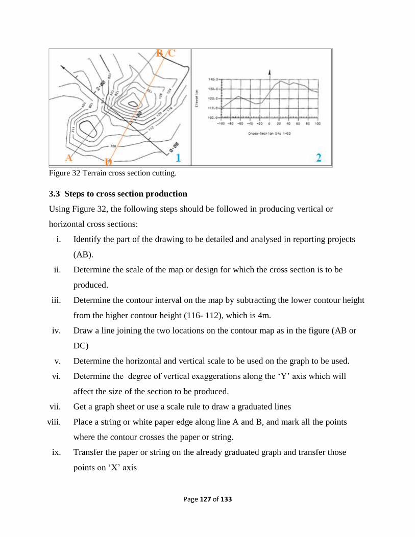
Page 127 of 133

Figure 32 Terrain cross section cutting.

3.3 Steps to cross section production

Using Figure 32, the following steps should be followed in producing vertical or

horizontal cross sections:

i. Identify the part of the drawing to be detailed and analysed in reporting projects

(AB).

ii. Determine the scale of the map or design for which the cross section is to be

produced.

iii. Determine the contour interval on the map by subtracting the lower contour height

from the higher contour height (116- 112), which is 4m.

iv. Draw a line joining the two locations on the contour map as in the figure (AB or

DC)

v. Determine the horizontal and vertical scale to be used on the graph to be used.

vi. Determine the degree of vertical exaggerations along the ‘Y’ axis which will

affect the size of the section to be produced.

vii. Get a graph sheet or use a scale rule to draw a graduated lines

viii. Place a string or white paper edge along line A and B, and mark all the points

where the contour crosses the paper or string.

ix. Transfer the paper or string on the already graduated graph and transfer those

points on ‘X’ axis

Page 128 of 133

x. Label the ‘Y’ axis as the height above sea level and the ‘X’ as the horizontal

distance on the ground.

xi. Now project the transferred points on ‘X’ axis to the appropriate height in relation

to the scale.

xii. Join all the height together with a line to show the configuration of the terrain as

indicated on the map

4.0 Conclusion

Terrain configuration analysis is very vital in environmental management as it helps in

proper developmental planning. Apart from descriptive analysis of a given topography,

section cutting detailing helps in assessing the degree of slopes and gradient in relation to

denudation activities and proffering management approached. A good knowledge of

terrain analysis will also help in inter-visibility assessment and decision making, hence

the relevancy in a course like this.


i. With suitable examples, what is relief in topographical analysis.

ii. Write short note on the following with illustrations: (Col, Saddle, and escarpment).

iii. From the contour provided, produce an annotated cross section between ‘A’ and ‘B’


Wise, S. (1995). Scanning Thematic Maps for Input to Geographic Information Systems,

Computers and Geosciences 21 (1): 7–29.


Shahab Fazal (2008). New GIS Basics. New Age International (P) Limited, Publishers

4835/24, Ansari Road, Daryaganj, New Delhi – 110002, ISBN (13) : 978-81-

224-2639-7

Visit us at www.newagepublishers.com

http://www.newagepublishers.com/

Page 129 of 133

UNIT 4: MAP ORIENTATION AND LAYOUTS

CONTENTS

1.0 Introduction

2.0 Objectives

3.0 Main Content

3.1 Map Orientation Techniques

3.2 Map Accuracy and Measurement

4.0 Conclusion



1.0 Introduction

Map orientation is very vital in map utilization especial for field work. A map is said to

be oriented when it is in a horizontal position with its north and south corresponding to

the north and south on the ground. The word "orient" is derived from Latin ‘oriens’

meaning east. In the Middle Ages, many maps were drawn with East at the top. This unit

will help student to understand know how to position maps with reference to the ground

position. This is similar to the map geo-referencing in satellite imageries.

2.0 Objectives

This unit is aimed at achieving the following:

i. Educate student on the meaning and purpose of map orientation.

ii. Expose student to map orientation techniques for practical field works.

iii. Acquit student with map accuracy and measurement determination.

iv. Student should at the end of the unit be able to orientate maps independently and

determine the accuracy of what they have done before external assessor.

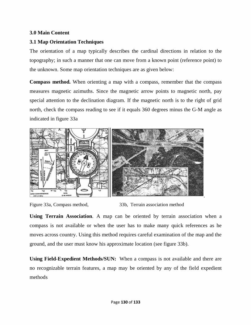
Page 130 of 133

3.0 Main Content

3.1 Map Orientation Techniques

The orientation of a map typically describes the cardinal directions in relation to the

topography; in such a manner that one can move from a known point (reference point) to

the unknown. Some map orientation techniques are as given below:

Compass method. When orienting a map with a compass, remember that the compass

measures magnetic azimuths. Since the magnetic arrow points to magnetic north, pay

special attention to the declination diagram. If the magnetic north is to the right of grid

north, check the compass reading to see if it equals 360 degrees minus the G-M angle as

indicated in figure 33a

.

Figure 33a, Compass method, 33b, Terrain association method

Using Terrain Association. A map can be oriented by terrain association when a

compass is not available or when the user has to make many quick references as he

moves across country. Using this method requires careful examination of the map and the

ground, and the user must know his approximate location (see figure 33b).

Using Field-Expedient Methods/SUN: When a compass is not available and there are

no recognizable terrain features, a map may be oriented by any of the field expedient

methods

Page 131 of 133

3.2 Map Accuracy and Measurements

Many factors besides resolution, influence how accurately features can be depicted which

includes the quality of data sources, the map scale, draftsman skills and the width of lines

drawn on the ground. A fine drafting pen will draw line’s 1/100 of an inch wide. Such a

line represents a corridor on the ground, which is almost 53 feet wide. In addition to this,

human drafting errors will occur and can be compounded by the quality of our map and

material sources. A map accurate for one purpose is often inaccurate for others since

accuracy is determined by the needs of the project as much as it is by the map itself.

Some measurements of a map’s accuracy are discussed below

i. Absolute accuracy of a map refers to the relationship between a geographic

position on a map (a street corner, for instance) and its real-world position

measured on the surface of the earth. Absolute accuracy is primarily important for

complex data requirements such as those for surveying and engineering-based

applications.

ii. Relative accuracy refers to the displacement between two points on a map (both

distance and angle), compared to the displacement of those same points in the real

world. Relative accuracy is often more important and easier to obtain than

absolute accuracy because users rarely need to know absolute positions. More

often, they need to find a position relative to some known landmark, which is

what relative accuracy provides. Users with simple data requirements generally

need only relative accuracy.

iii. Attribute accuracy refers to the precision of the attribute database linked to the

map’s features. For example, if the map shows road classifications, are they

correct? If it shows street addresses, how accurate are they? Attribute accuracy is

most important to users with complex data requirements.

iv. A map’s Currency refers to how up-to-date it is. Currency is usually expressed in

terms of a revision date, but this information is not always easy to find.

Page 132 of 133

v. A map is Complete, if it includes all the features a user would expect it to contain.

For example, does a street map contain all the streets? Completeness and currency

usually are related because a map becomes less complete as it gets older.

The most important issue to remember about map accuracy is that the more accurate the

map, the more it costs in time and money to develop. For example, digital maps with

coordinate accuracy of about 100 feet can be purchased inexpensively. If 1-foot accuracy

is required, a custom survey is often the only way to get it, which drives up data-

acquisition costs by many orders of magnitude and can significantly delay project

implementation over a prolong period of time.

4.0 Conclusion

Map production is not as easy as its utilization because the inputs and output accuracy is

of utmost importance to the purpose of the map. The quality of maps and speed of

production has change over the years with the advancement in computer software and

remote sensing technology.


i. Using the topographic map given, develop the cross section between point C and

D and discuss the result.

ii. With reference to Ptolemy’s map of the world, discuss the origin of map

production

iii. Discuss five types of map and their uniqueness.

iv. What is map accuracy and how it can be measure.


Robinson, A.H., Sale, R.D., Morrison, J.L., and Muechrcke, P.C. (1984). Elements of

Cartography, 5th edition, Wiley, New York.

Rhind, D. (1979). Computer-Aided Cartography, Trans. Inst, British Geographers,

NS2. pp 7

Euckar, T.K., and Chrisman, N. (1975). "Cartographic Data Structures". The American

Page 133 of 133

Cartographer, Vol. 2, No.1, pp 55-69.

Monmonier, M., and Schnell, G.A. (1988). Map Appreciation. Englewood Cliffs,

Prentice Hall, New Jersey.

Documents

Course Guide on Introduction to Practical Geography Course