Course: DD2427 - Exercise Set 5

In this exercise we will model skin colour with a multi-variate Gaussian. Ifx is the vector that contains the data associated with a pixel’s colour (itsrgb value for instance) then we assume

p(x | skin pixel) =1

(2π)d2 |Σs|

12

exp(−1

2(x− µs)

T Σ−1s (x− µs)

)(1)

However, the values of the parameters (µs,Σs) defining this model are un-known. These need to be learned from training data.

Exercise 1: Learning the multi-variate Gaussian

To learn the parameters of the multi-variate Gaussian, we require trainingdata. Fortunately, lots of people have built databases of colour images ofhuman faces and have made them available publicly. We will use imagesavailable at http://vis-www.cs.umass.edu/lfw/. The complete databasecontains a large number of images, far more than needed for our purposestherefore you should just download a small proportion of them available at:http://vis-www.cs.umass.edu/lfw/lfw-bush.tgz. You can use gunzipand tar to extract the images. Place these images in a separate directory.You will use these to learn the colour of skin pixels and in fact you will onlyrequire a small number of them to learn the multi-variate Gaussian model.

In the images you have downloaded the centre of the face is at the centreof the image and composes roughly 30% of the area of the image (exactdetails are available at the face database web-site). If you grab the pixelsin a relatively small rectangular region centred at the centre of the image,then you can be quite sure that these will be skin coloured pixels. Your firsttask is to write a function that takes as input the name of the file and pa number in [0,1]. The function then grabs the centre rectangular regionof size (floor(p*W))(floor(p*H)) from the image where W and H are thewidth and height of the original image. Call this function via

function cim = GrabCenterPixels(im fname, p);

Note that cim will be an array of size p*H×p*W×3. We can turn the pixeldata in this array into a more useful shape with the following command:

rgb data = reshape(cim, [size(cim,1)*size(cim,2), 3]);

This turns the rgb data in cim into the array, rgb data, of size size(cim,1)*size(cim,2)×3.Each row of the matrix corresponds to the rgb value of one skin pixel. The

1

first column of this array corresponds to the r data, the second column theg data and the third to the b blue data.

The next task is to read in n (∼20) of the face images you downloaded, fromeach image extract the central pixels with the function you’ve just written,keep a record of these skin pixels and then compute the mean value of thergb pixel values and the covariance of these pixels. Use the Matlab functionsmean and cov to compute these quantities. Perform this task in the function

function [mu, Sigma] = TrainColourModel(DirName, n);

which takes as input the name of the directory containing the face imagesand the number, n, of images to be used for training. The output will bethe mean vector, mu (size 3 × 1), of the rgb pixel data you have extractedand its covariance, Sigma (size 3 × 3).

Matlab Tip Remember you can concatenate an array A of size n a×3 andanother array B of size n b×3 into a new array of size n a + n b×3 with thecommand: C = [A;B];

When I performed this task with n=20, p=.2 and used the first n images, Icalculated mu and Sigma as:

mu =[176.91 129.18 103.88

], Sigma = 1.0e+ 03 ∗

1.7264 1.4316 1.44791.4316 1.4268 1.44981.4479 1.4498 1.5935

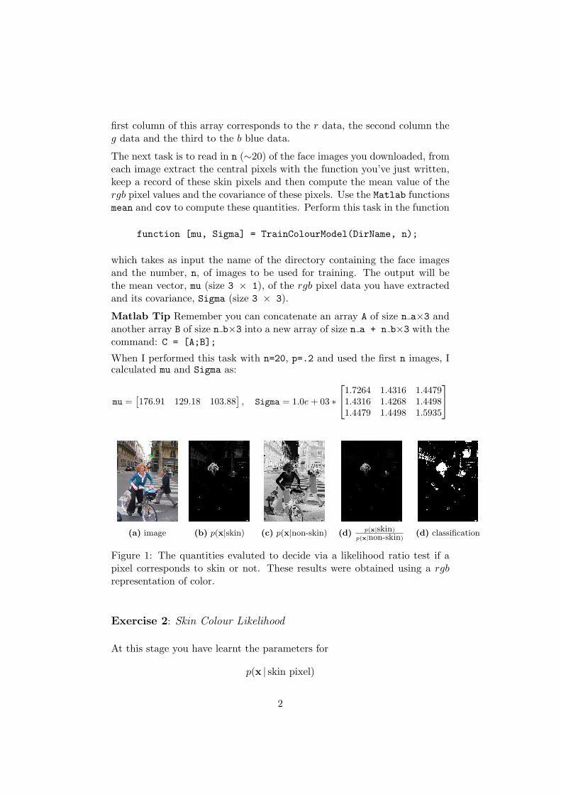
(a) image (b) p(x|skin) (c) p(x|non-skin) (d) p(x|skin)

p(x|non-skin)(d) classification

Figure 1: The quantities evaluted to decide via a likelihood ratio test if apixel corresponds to skin or not. These results were obtained using a rgbrepresentation of color.

Exercise 2: Skin Colour Likelihood

At this stage you have learnt the parameters for

p(x | skin pixel)

2

where x is a pixel’s rgb value. The next task is to investigate the useful-ness of this model. Load the image bike small.jpg. For each pixel inbike small.jpg we want to compute p( x | skin pixel) as defined in equa-tion (1) where x contains the rgb value of the pixel and µs = mu and Σs =Sigma. The Matlab functions det and inv compute the determinant andinverse of a matrix. Write a function that evaluates equation (1) for a setof points. These points are contained in the array xs of size N×d where N isthe number of points and d is the number of points.

function lvals = GaussLikelihood(xs, mean, Sigma)

Matlab Tip If lvals is an array of size N×1, then it can be turned into anarray of dimensions equal to the test image im with the command:

im lvals = reshape(lvals, [size(im, 1), size(im, 2)]);

Run your new function on the rgb pixel values obtained from the imagebike small.jpg. Then display the results. You should get something as infigure 1 (a).

Exercise 3: Use HSV colour model

Is the rgb colour model the best represention of colour for this task of de-tecting skin pixels ? In this exercise we will investigate using the HSV colourmodel instead. Fortunately, we can reuse, with only minor additions, mostof the code you’ve already written. Before you start note that as the hue of acolour is an angle, it is easier to let x = (cos(hue), sin(hue), saturation, value)to avoid the nuisance of 0◦ = 360◦. The four things you have to do are

• Amend the function TrainColourModel to take an extra input param-eter. This will be a flag, m, to indicate which colour model you areusing. Thus it becomes:

function [mu, Sigma] = TrainColourModel(DirName, n, m);

Once you have grabbed the training data then if m indicates you areusing the HSV colour model then convert the rgb pixel data into hsvpixel data via the Matlab command rgb2hsv.

• From the hsv data create the augmented hsv data where its first col-umn is cos(hue), the second sin(hue), the third saturation and the lastvalue.

• The rest of the function should work as before if you haven’t hardcoded in the fact that your feature has dimension 3 and you shouldget a new mean vector and covariance matrix.

3

• Convert the test image pixels into the same form of the HSV dataas the training data and then compute the likelihood of each pixelcorresponds to skin using GaussLikelihood. Display the result. Itshould look as in figure 1 (c).

Exercise 4: Likelihood ratio test to classify pixels as skin or non skin

Finally you can classify a pixel in your image as skin if :

p(x | skin pixel)p(x |non-skin pixel)

> 1 (2)

as in the liklihood ratio test for classes with equal priors.

However, to do this it is necessary to have some model/representation ofp(x | non-skin pixel). There are obviously lots of options for this. One sug-gestion is to use a multi-variate Gaussian as in the case of skin pixels. How-ever, if you use this, training data (lots of non-skin pixels) is required fromwhich you can learn the parameters of the Gaussian. Luckily for you I havedownloaded a few such images from flickr for this task.

Download these from the course website and put them into a separate direc-tory. Now you can reuse the function TrainColourModel, though you maywant to grab the whole image as opposed to a central rectangle, to obtain amean vector and covariance for the distribution describing the colour pixelsfor the background (or at least our sparsely sampled version of the back-ground). If you run GaussLikelihood on the pixel data obtained from theimage bike small.jpg you should get an image that look as figure 1(c), foran rgb representation and as figure 2(c), for a hsv representation.

If you plot the ratio of the likelihood values for the skin and non-skin modelsyou should get results as in figures 1(d) and 2(d). Finally, you can create animage from the binary classification rule based on equation (). To do this,create an array full of zeros, Matlab command zeros, and set an entry toone if for that pixel its likelihood of being skin coloured is greater than thatof being non-skin coloured. The results you get should be similar to thosein figures 1(e) and 2(e) depending on which colour model you use.

It may be useful to save the different mean vectors and covariance matricesyou have calculated and to gather the commands you used to classify thepixels in an image into one function. It can be called with an image arrayas input and returns the binary image of classified pixels:

function bim = SkinClassifier(im)

4

Mathematical Tip: When computing the likelihood, you can actually getby with just computing the log-likelihood. That is just compute

log( p(x | skin pixel) ) = −d2

log( 2π )− 12

log(|Σs|)−12

(x− µs)T Σ−1s (x− µs)

The classification can then be computed with this test:

log( p(x | skin pixel) )− log( p(x | non-skin pixel) ) > 0 (3)

This avoids computing the relatively expensive exp function and also is morenumerically stable for values of x that produce very small likelihood values.For this exercise you can use either the likelihood or the log-likelihood. But,in general, it is probably better to use the log-likelohood values.

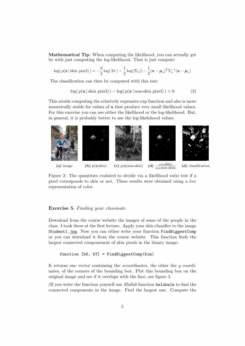
(a) image (b) p(x|skin) (c) p(x|non-skin) (d) p(x|skin)

p(x|non-skin)(d) classification

Figure 2: The quantities evaluted to decide via a likelihood ratio test if apixel corresponds to skin or not. These results were obtained using a hsvrepresentation of color.

Exercise 5: Finding your classmate

Download from the course website the images of some of the people in theclass. I took these at the first lecture. Apply your skin classifier to the imageStudent1.jpg. Now you can either write your function FindBiggestCompor you can download it from the course website. This function finds thelargest connected componenent of skin pixels in the binary image:

function [bX, bY] = FindBiggestComp(bim)

It returns one vector containing the xcoordinates, the other the y coordi-nates, of the corners of the bounding box. Plot this bounding box on theoriginal image and see if it overlaps with the face, see figure 3.

(If you write the function yourself use Matlab function bwlabeln to find theconnected components in the image. Find the largest one. Compute the

5

smallest rectangle that encloses this connected component, the boundingbox.)

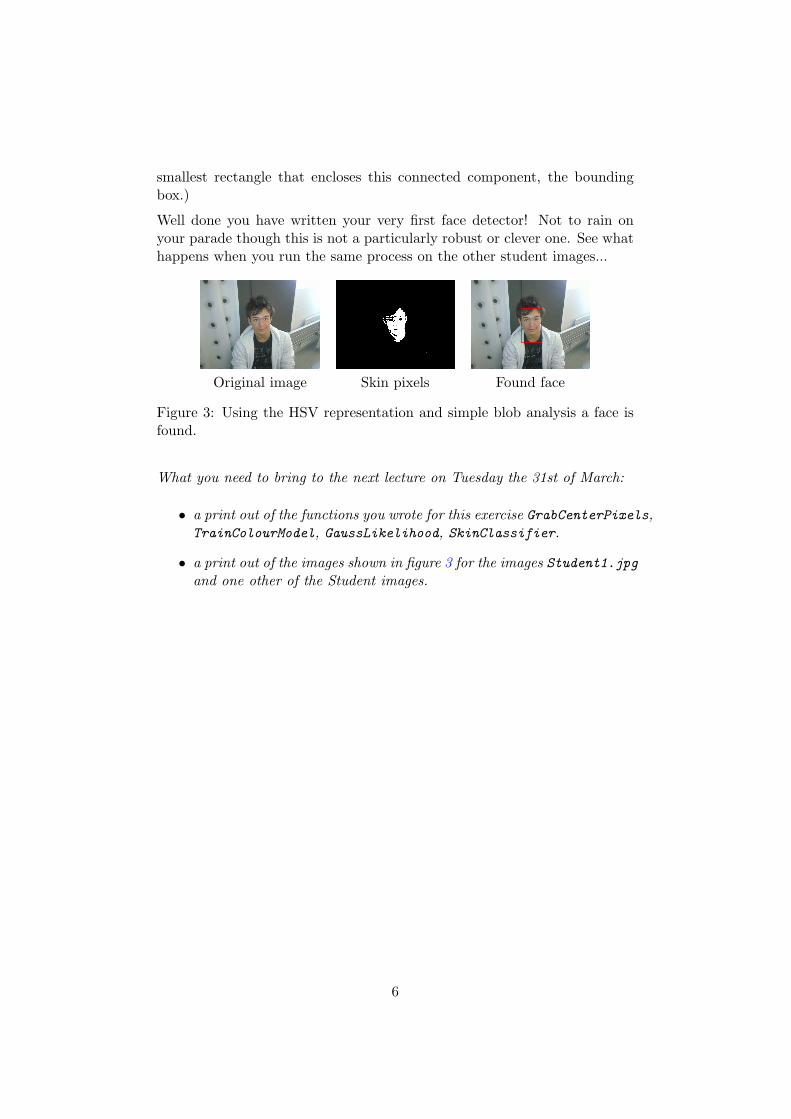
Well done you have written your very first face detector! Not to rain onyour parade though this is not a particularly robust or clever one. See whathappens when you run the same process on the other student images...

Original image Skin pixels Found face

Figure 3: Using the HSV representation and simple blob analysis a face isfound.

What you need to bring to the next lecture on Tuesday the 31st of March:

• a print out of the functions you wrote for this exercise GrabCenterPixels,TrainColourModel, GaussLikelihood, SkinClassifier.

• a print out of the images shown in figure 3 for the images Student1.jpgand one other of the Student images.

6