Embed Size (px)
Citation preview
Stavros Petridis Machine Learning (course 395)
Course 395: Machine Learning - LecturesLecture 1-2: Concept Learning (M. Pantic)
Lecture 3-4: Decision Trees & CBC Intro (M. Pantic & S. Petridis)
Lecture 5-6: Evaluating Hypotheses (S. Petridis)
Lecture 7-8: Artificial Neural Networks I (S. Petridis)
Lecture 9-10: Artificial Neural Networks II (S. Petridis)
Lecture 11-12: Artificial Neural Networks III (S. Petridis)
Lecture 13-14: Genetic Algorithms (M. Pantic)
Stavros Petridis Machine Learning (course 395)
Neural Networks
Reading:
• Machine Learning (Tom Mitchel) Chapter 4
• Pattern Classification (Duda, Hart, Stork) Chapter 6
(chapters 6.1, 6.2, 6.3, 6.8)
• http://neuralnetworksanddeeplearning.com/
(great online book)
• Deep Learning (Goodfellow, Bengio, Courville)
Coursera classes
- Machine Learning by Andrew Ng
- Neural Networks by Hinton

Stavros Petridis Machine Learning (course 395)
History
• 1st generation Networks: Perceptron 1957 – 1969
- Perceptron is useful only for examples that are linearly separable
• 2nd generation Networks: Feedforward Networks and
other variants, beginning of 1980s to middle / end of
1990s
- Difficult to train, many parameters, similar performance to SVMs
• 3rd generation Networks: Deep Networks 2006 - ?
- New approach to train networks with multiple layers
- State of the art in object recognition / speech recognition (since 2012)
Stavros Petridis Machine Learning (course 395)
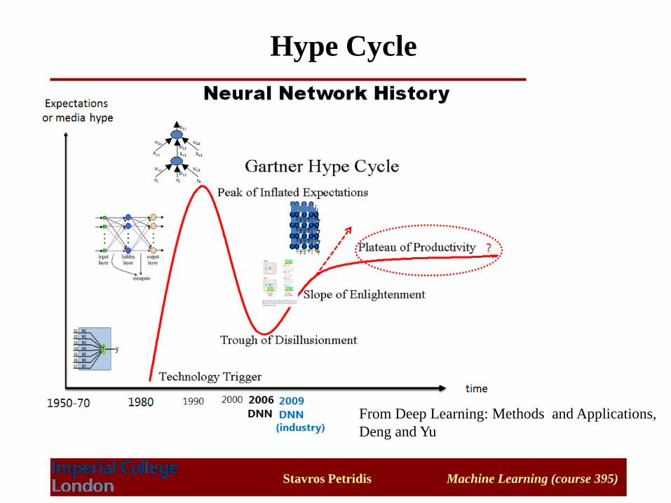
Hype Cycle
From Deep Learning: Methods and Applications,
Deng and Yu
Stavros Petridis Machine Learning (course 395)
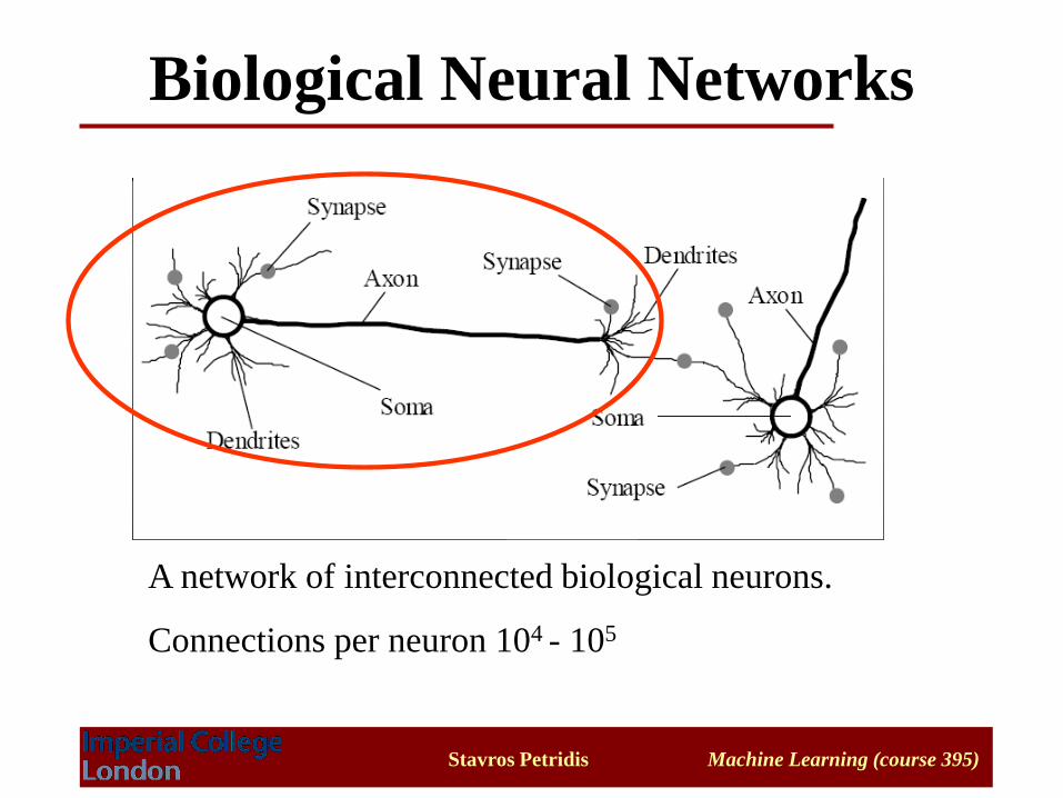
Biological Neural Networks
A network of interconnected biological neurons.
Connections per neuron 104 - 105
Stavros Petridis Machine Learning (course 395)
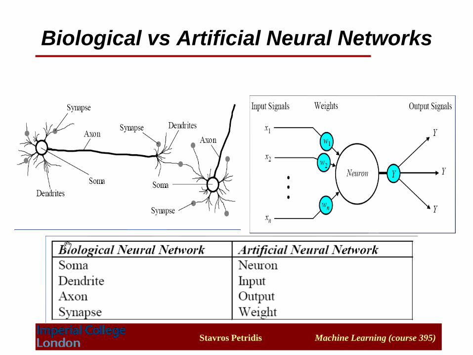
Biological vs Artificial Neural Networks
Stavros Petridis Machine Learning (course 395)
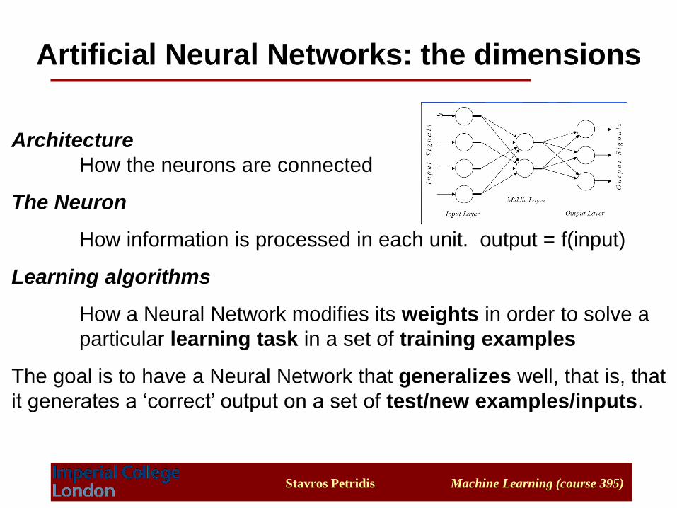
Architecture
How the neurons are connected
The Neuron
How information is processed in each unit. output = f(input)
Learning algorithms
How a Neural Network modifies its weights in order to solve a
particular learning task in a set of training examples
The goal is to have a Neural Network that generalizes well, that is, that
it generates a ‘correct’ output on a set of test/new examples/inputs.
Artificial Neural Networks: the dimensions
Stavros Petridis Machine Learning (course 395)
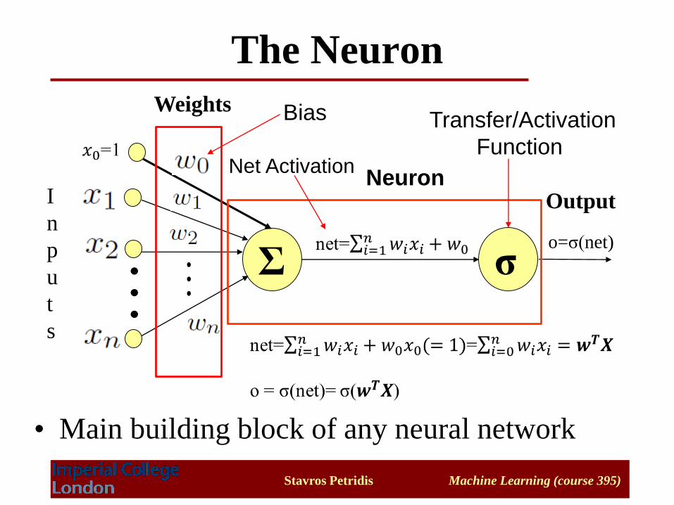
The Neuron
Σ
I
n
p
u
t
s
Output
Bias
σo=σ(net)
Neuron
Weights
• Main building block of any neural network
Net Activation
Transfer/Activation
Function
Stavros Petridis Machine Learning (course 395)
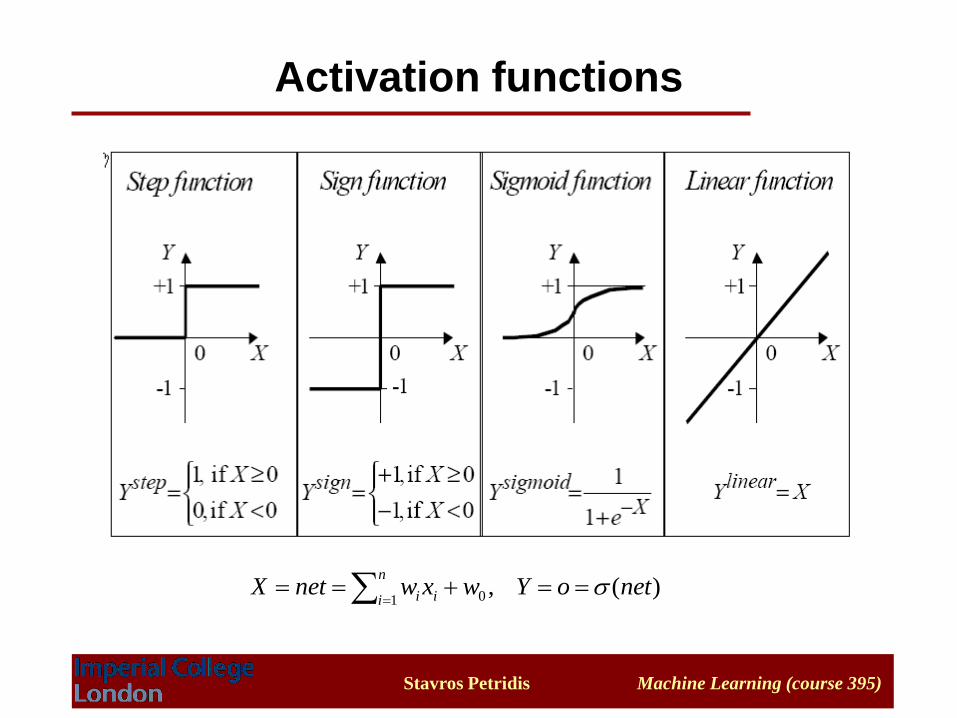
Activation functions
)(,1 0 netoYwxwnetX
n
i ii
Stavros Petridis Machine Learning (course 395)
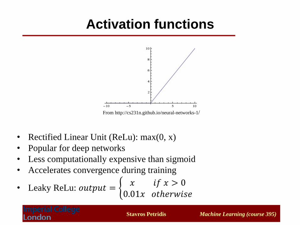
Activation functions
From http://cs231n.github.io/neural-networks-1/
• Rectified Linear Unit (ReLu): max(0, x)
• Popular for deep networks
• Less computationally expensive than sigmoid
• Accelerates convergence during training
• Leaky ReLu: 𝑜𝑢𝑡𝑝𝑢𝑡 = ቊ𝑥 𝑖𝑓 𝑥 > 0
0.01𝑥 𝑜𝑡ℎ𝑒𝑟𝑤𝑖𝑠𝑒
Stavros Petridis Machine Learning (course 395)
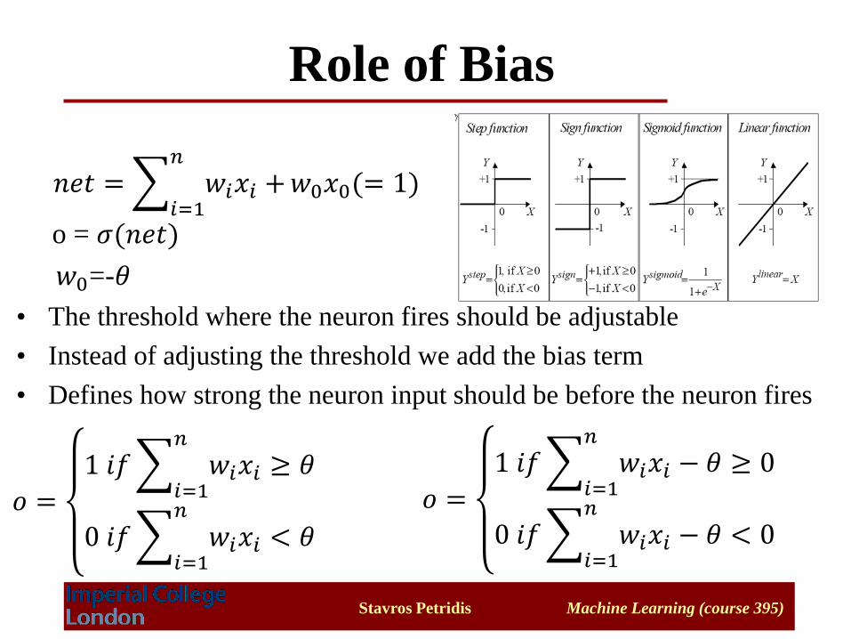
Role of Bias
• The threshold where the neuron fires should be adjustable
• Instead of adjusting the threshold we add the bias term
• Defines how strong the neuron input should be before the neuron fires
𝑛𝑒𝑡 =𝑖=1
𝑛
𝑤𝑖𝑥𝑖 +𝑤0𝑥0(= 1)
o = 𝜎(𝑛𝑒𝑡)
𝑜 =
1 𝑖𝑓𝑖=1
𝑛
𝑤𝑖𝑥𝑖 ≥ 𝜃
0 𝑖𝑓𝑖=1
𝑛
𝑤𝑖𝑥𝑖 < 𝜃
𝑜 =
1 𝑖𝑓𝑖=1
𝑛
𝑤𝑖𝑥𝑖 − 𝜃 ≥ 0
0 𝑖𝑓𝑖=1
𝑛
𝑤𝑖𝑥𝑖 − 𝜃 < 0
𝑤0=-𝜃
Stavros Petridis Machine Learning (course 395)
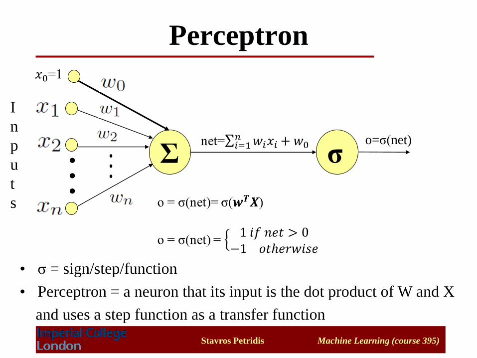
Perceptron
Σ
I
n
p
u
t
s
σo=σ(net)
• σ = sign/step/function
• Perceptron = a neuron that its input is the dot product of W and X
and uses a step function as a transfer function
Stavros Petridis Machine Learning (course 395)
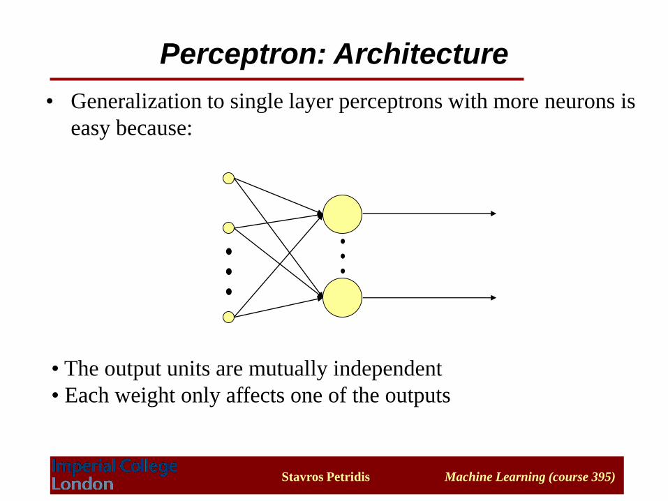
• Generalization to single layer perceptrons with more neurons is
easy because:
• The output units are mutually independent
• Each weight only affects one of the outputs
Perceptron: Architecture
Stavros Petridis Machine Learning (course 395)
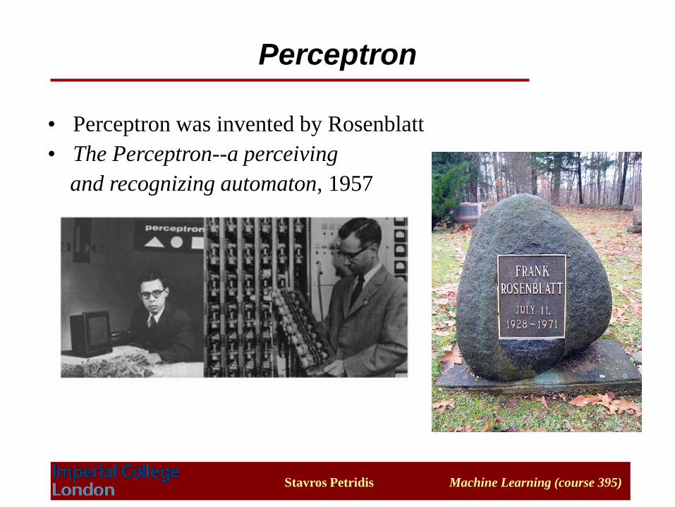
• Perceptron was invented by Rosenblatt
• The Perceptron--a perceiving
and recognizing automaton, 1957
Perceptron

Stavros Petridis Machine Learning (course 395)
Perceptron: Example 1 - AND
• x1 = 1, x2 = 1 net = 20+20-30=10 o = σ(10) = 1
• x1 = 0, x2 = 1 net = 0+20-30 =-10 o = σ(-10) = 0
• x1 = 1, x2 = 0 net = 20+0-30 =-10 o = σ(-10) = 0
• x1 = 0, x2 = 0 net = 0+0-30 =-30 o = σ(-10) = 0
Σ σo=σ(net)
Stavros Petridis Machine Learning (course 395)
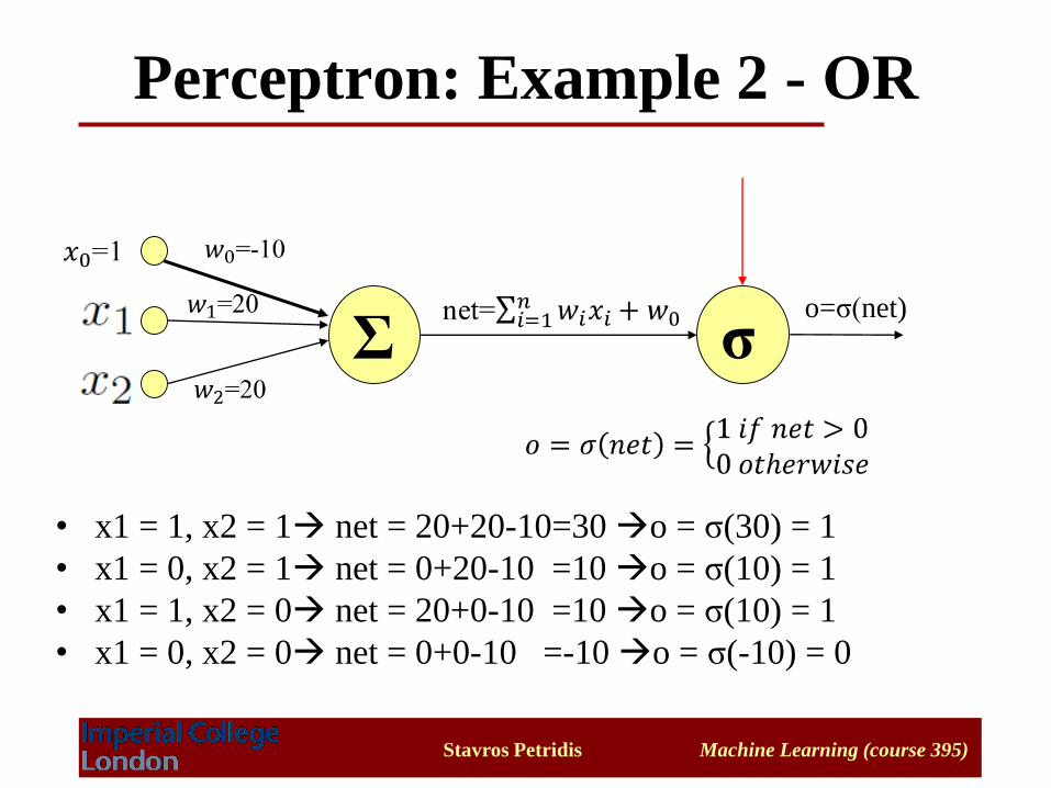
Perceptron: Example 2 - OR
• x1 = 1, x2 = 1 net = 20+20-10=30 o = σ(30) = 1
• x1 = 0, x2 = 1 net = 0+20-10 =10 o = σ(10) = 1
• x1 = 1, x2 = 0 net = 20+0-10 =10 o = σ(10) = 1
• x1 = 0, x2 = 0 net = 0+0-10 =-10 o = σ(-10) = 0
Σ σo=σ(net)
Stavros Petridis Machine Learning (course 395)
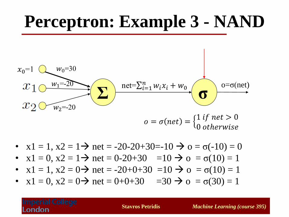
Perceptron: Example 3 - NAND
• x1 = 1, x2 = 1 net = -20-20+30=-10 o = σ(-10) = 0
• x1 = 0, x2 = 1 net = 0-20+30 =10 o = σ(10) = 1
• x1 = 1, x2 = 0 net = -20+0+30 =10 o = σ(10) = 1
• x1 = 0, x2 = 0 net = 0+0+30 =30 o = σ(30) = 1
Σ σo=σ(net)
Stavros Petridis Machine Learning (course 395)
• Given training examples of classes A1, A2 train the
perceptron in such a way that it classifies correctly the
training examples:
– If the output of the perceptron is 1 then the input is
assigned to class A1 (i.e. if )
– If the output is 0 then the input is assigned to class A2
• Geometrically, we try to find a hyper-plane that separates the
examples of the two classes. The hyper-plane is defined by the
linear function
Perceptron for classification
Stavros Petridis Machine Learning (course 395)
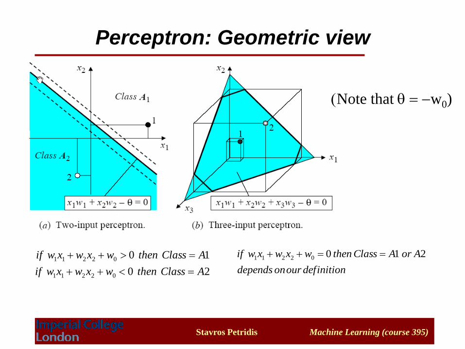
Perceptron: Geometric view
(Note that q -w0)
20
10
02211
02211
AClassthenwxwxwif
AClassthenwxwxwif
definitionourondepends
AorAClassthenwxwxwif 21002211
Stavros Petridis Machine Learning (course 395)
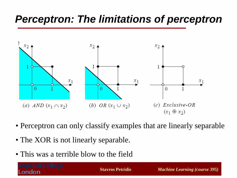
Perceptron: The limitations of perceptron
• Perceptron can only classify examples that are linearly separable
• The XOR is not linearly separable.
• This was a terrible blow to the field
Stavros Petridis Machine Learning (course 395)
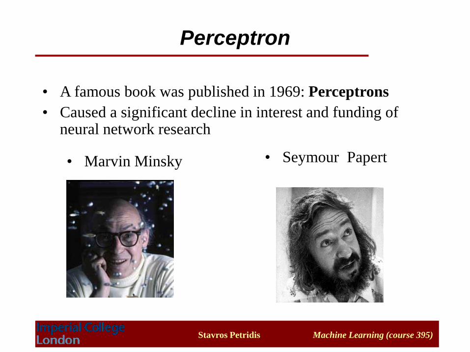
• Marvin Minsky • Seymour Papert
• A famous book was published in 1969: Perceptrons
• Caused a significant decline in interest and funding of neural network research
Perceptron
Stavros Petridis Machine Learning (course 395)
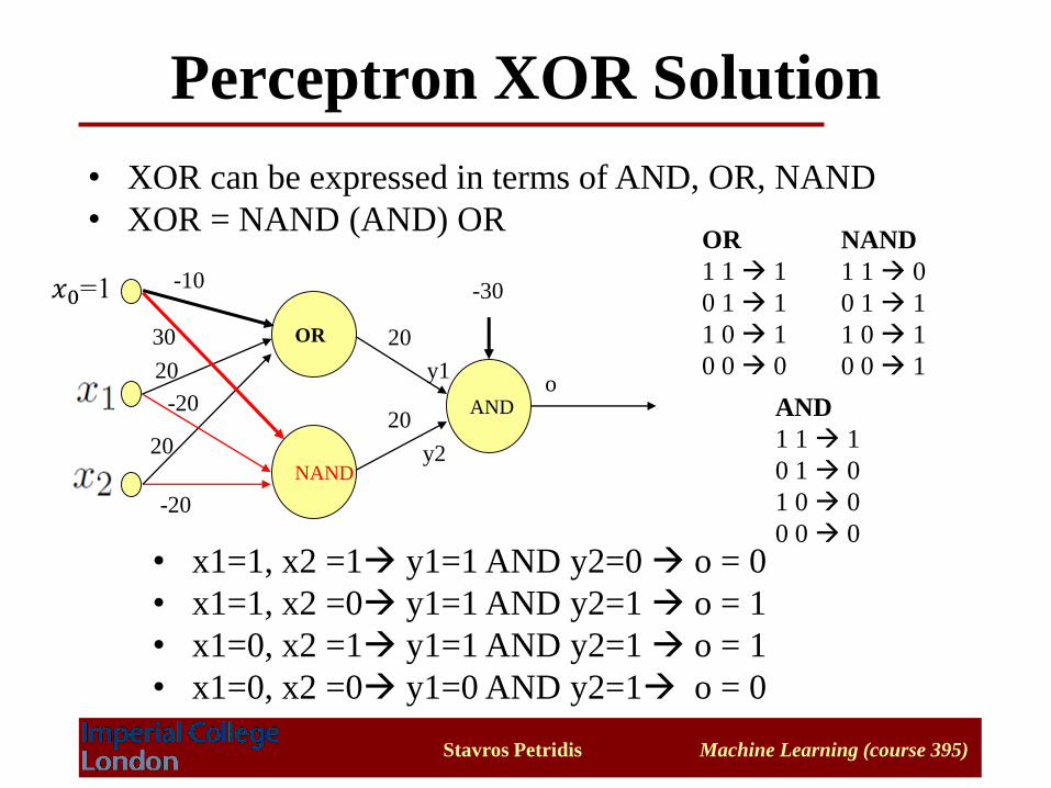
Perceptron XOR Solution
• XOR can be expressed in terms of AND, OR, NAND
• XOR = NAND (AND) OR
AND
1 1 1
0 1 0
1 0 0
0 0 0
OR
1 1 1
0 1 1
1 0 1
0 0 0
NAND
1 1 0
0 1 1
1 0 1
0 0 1
OR
20
20
-10
NAND
-20
-20
30
20AND
20
-30
y1
y2
o
• x1=1, x2 =1 y1=1 AND y2=0 o = 0
• x1=1, x2 =0 y1=1 AND y2=1 o = 1
• x1=0, x2 =1 y1=1 AND y2=1 o = 1
• x1=0, x2 =0 y1=0 AND y2=1 o = 0
Stavros Petridis Machine Learning (course 395)
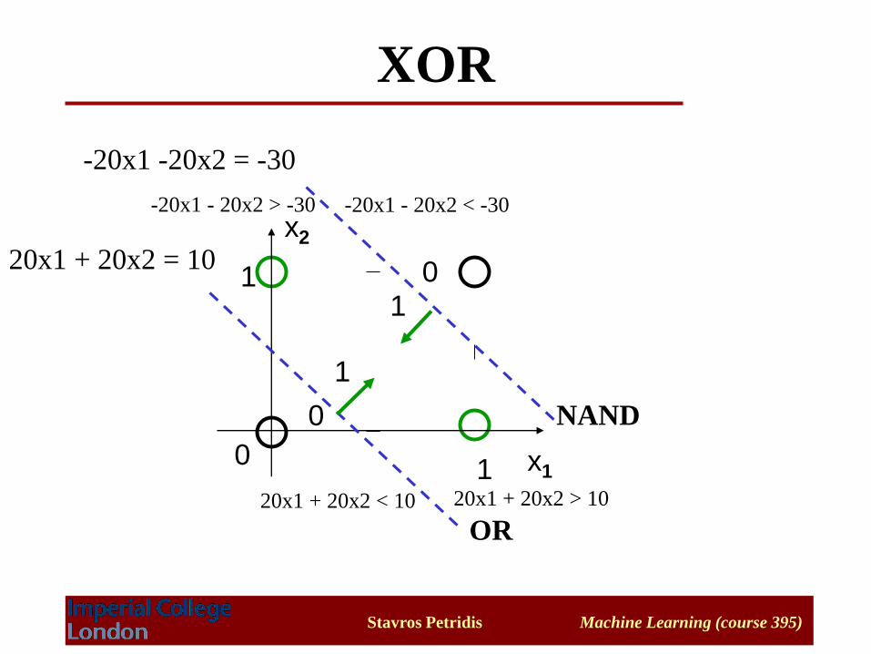
XOR
1
01
x2
x1
OR
NAND
1
1
0
020x1 + 20x2 = 10
-20x1 -20x2 = -30
20x1 + 20x2 < 10 20x1 + 20x2 > 10
-20x1 - 20x2 < -30-20x1 - 20x2 > -30
Stavros Petridis Machine Learning (course 395)
Input
layer
Output
layer
Hidden Layer
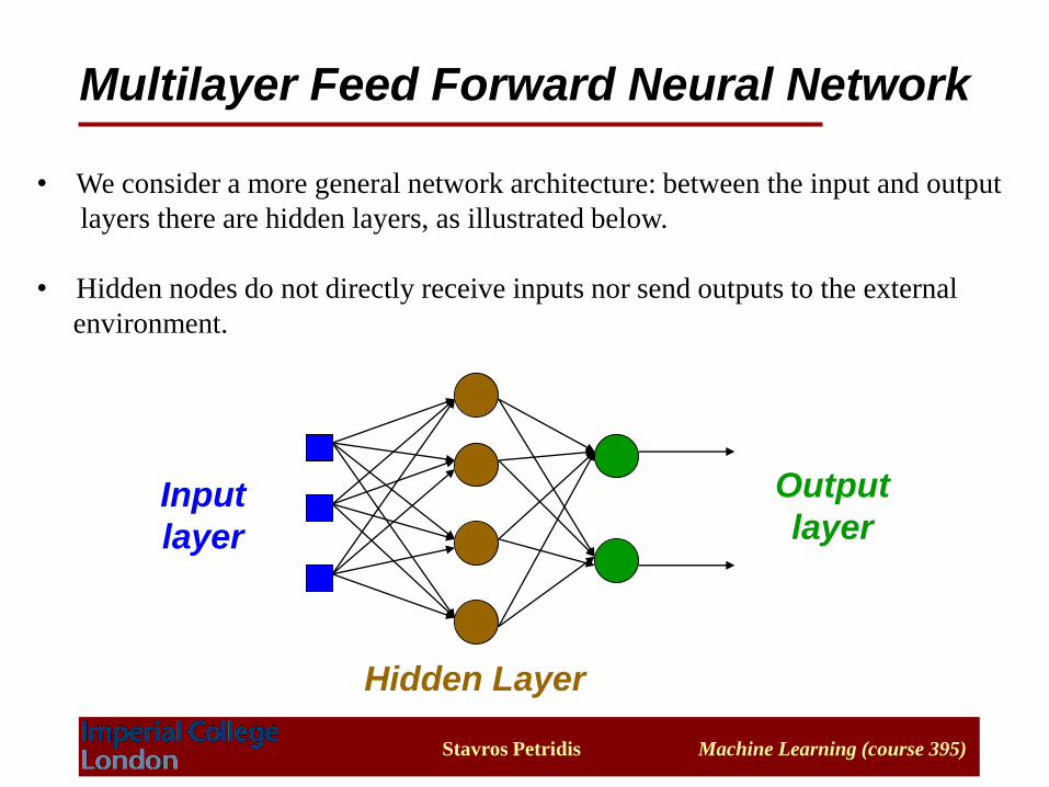
• We consider a more general network architecture: between the input and output
layers there are hidden layers, as illustrated below.
• Hidden nodes do not directly receive inputs nor send outputs to the external
environment.
Multilayer Feed Forward Neural Network

Stavros Petridis Machine Learning (course 395)
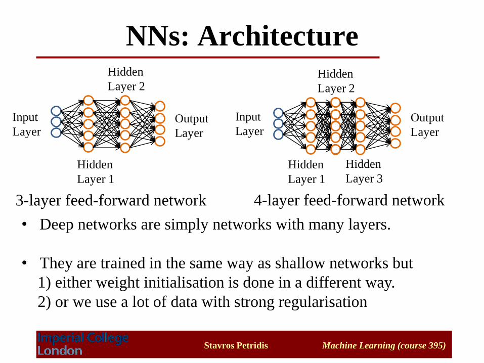
NNs: Architecture
Input
Layer
Hidden
Layer 1
Hidden
Layer 2
Output
Layer
Hidden
Layer 1
Hidden
Layer 2
Hidden
Layer 3
Output
Layer
Input
Layer
Feedback
Connection
3-layer feed-forward network 4-layer feed-forward network
4-layer recurrent network – Difficult to train
• The input layer does
not count as a layer
Stavros Petridis Machine Learning (course 395)
NNs: Architecture
Input
Layer
Hidden
Layer 1
Hidden
Layer 2
Output
Layer
Hidden
Layer 1
Hidden
Layer 2
Hidden
Layer 3
Output
Layer
Input
Layer
3-layer feed-forward network 4-layer feed-forward network
• Deep networks are simply networks with many layers.
• They are trained in the same way as shallow networks but
1) either weight initialisation is done in a different way.
2) or we use a lot of data with strong regularisation
Stavros Petridis Machine Learning (course 395)
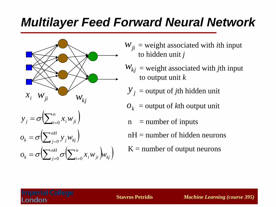
Multilayer Feed Forward Neural Network
jiwkjwix
jiw = weight associated with ith input
to hidden unit j
kjw = weight associated with jth input
to output unit k
jy
ko
= output of jth hidden unit
= output of kth output unit
(
n
i jiij wxy0
(
nH
j kjjk wyo0
n = number of inputs
nH = number of hidden neurons
K = number of output neurons ( (
nH
j kj
n
i jiik wwxo0 0
Stavros Petridis Machine Learning (course 395)
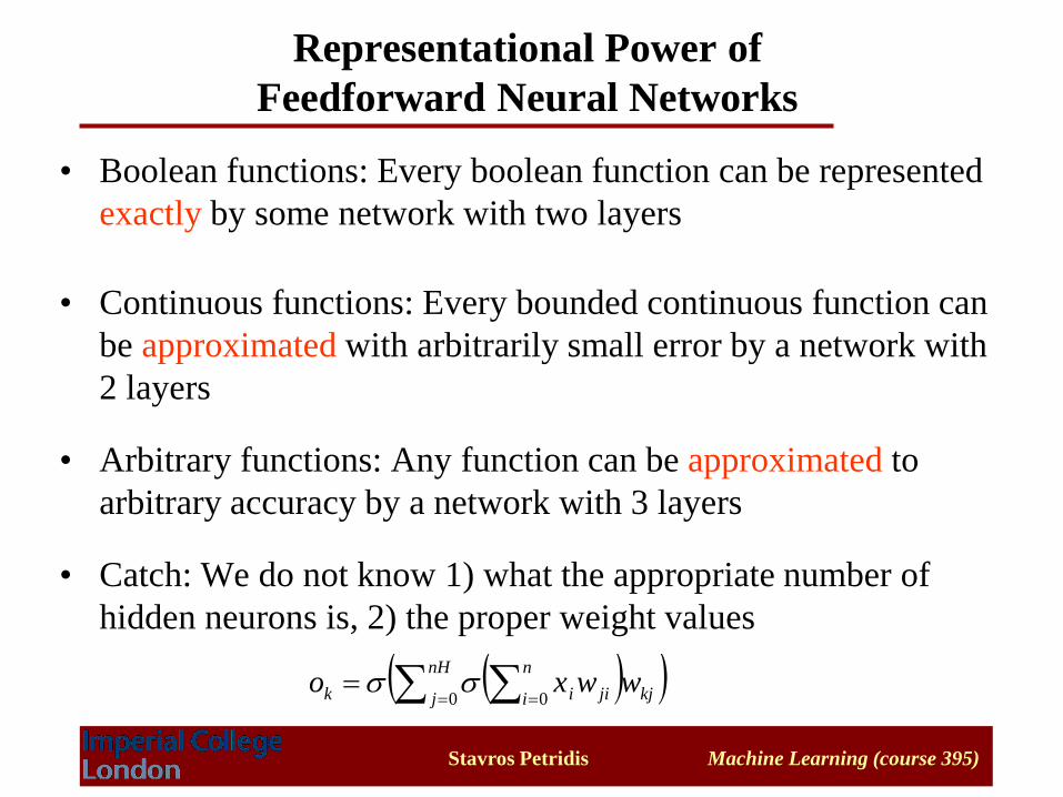
Representational Power of
Feedforward Neural Networks
• Boolean functions: Every boolean function can be represented
exactly by some network with two layers
• Continuous functions: Every bounded continuous function can
be approximated with arbitrarily small error by a network with
2 layers
• Arbitrary functions: Any function can be approximated to
arbitrary accuracy by a network with 3 layers
• Catch: We do not know 1) what the appropriate number of
hidden neurons is, 2) the proper weight values
( (
nH
j kj
n
i jiik wwxo0 0
Stavros Petridis Machine Learning (course 395)
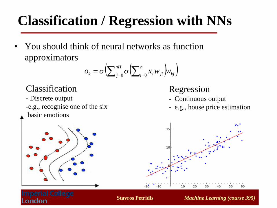
Classification / Regression with NNs
• You should think of neural networks as function
approximators
( (
nH
j kj
n
i jiik wwxo0 0
Classification- Discrete output
-e.g., recognise one of the six
basic emotions
Regression- Continuous output
- e.g., house price estimation
Stavros Petridis Machine Learning (course 395)
Output Representation
• Binary Classification
Target Values (t): 0 or -1 (negative) and 1 (positive)
• Regression
Target values (t): continuous values [-inf, +inf]
• Ideally o ≈ t
( (
nH
j kj
n
i jiik wwxo0 0
Stavros Petridis Machine Learning (course 395)
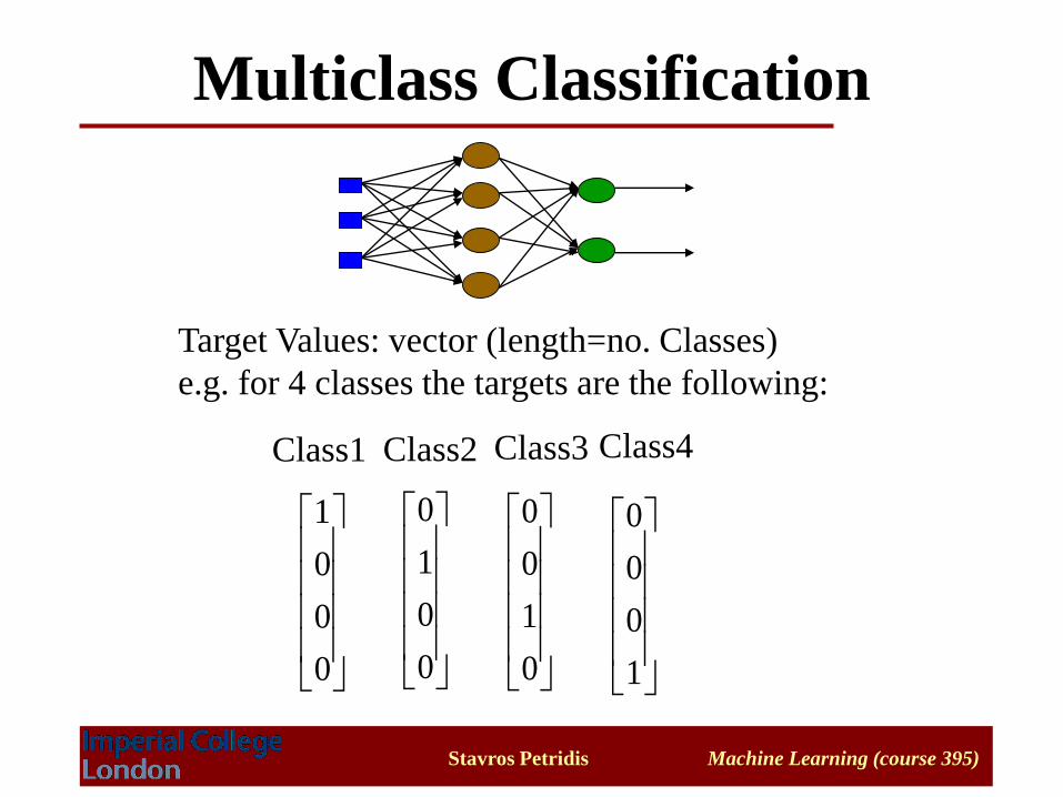
Multiclass Classification
Target Values: vector (length=no. Classes)
e.g. for 4 classes the targets are the following:
0
0
0
1
0
0
1
0
0
1
0
0
1
0
0
0
Class1 Class3Class2 Class4
Stavros Petridis Machine Learning (course 395)
Training
• We have assumed so far that we know the weight
values
• We are given a training set consisting of inputs and
targets (X, T)
• Training: Tuning of the weights (w) so that for each
input pattern (x) the output (o) of the network is close
to the target values (t).
( (
nH
j kj
n
i jii wwxo0 0
o ≈ t
Stavros Petridis Machine Learning (course 395)
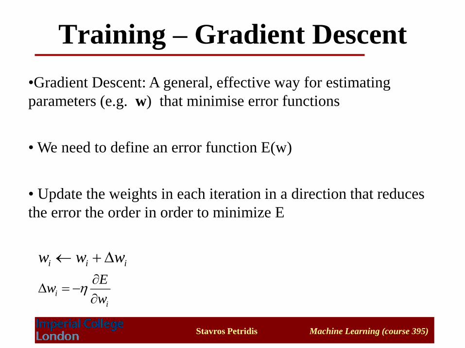
Training – Gradient Descent
•Gradient Descent: A general, effective way for estimating
parameters (e.g. w) that minimise error functions
• We need to define an error function E(w)
• Update the weights in each iteration in a direction that reduces
the error the order in order to minimize E
iii www
i
iw
Ew
-
Stavros Petridis Machine Learning (course 395)
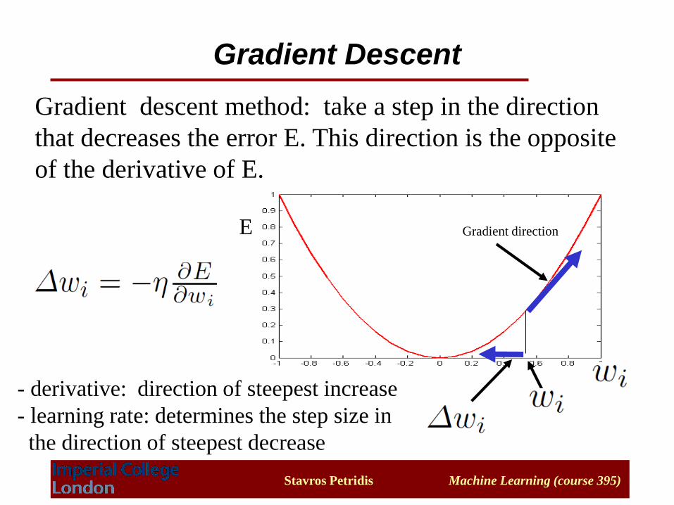
Gradient descent method: take a step in the direction
that decreases the error E. This direction is the opposite
of the derivative of E.
Gradient directionE
Gradient Descent
- derivative: direction of steepest increase
- learning rate: determines the step size in
the direction of steepest decrease
Stavros Petridis Machine Learning (course 395)
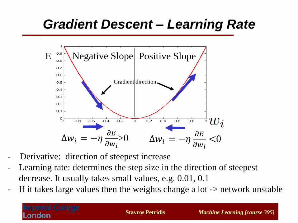
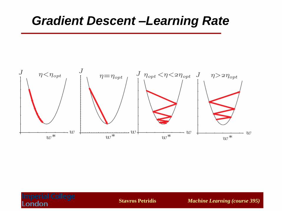
Gradient Descent – Learning Rate
- Derivative: direction of steepest increase
- Learning rate: determines the step size in the direction of steepest
decrease. It usually takes small values, e.g. 0.01, 0.1
- If it takes large values then the weights change a lot -> network unstable
∆𝑤𝑖 = −𝜂𝜕𝐸
𝜕𝑤𝑖>0 ∆𝑤𝑖 = −𝜂
𝜕𝐸
𝜕𝑤𝑖<0
E
Gradient direction
Positive SlopeNegative Slope
Stavros Petridis Machine Learning (course 395)
Gradient Descent –Learning Rate
Stavros Petridis Machine Learning (course 395)
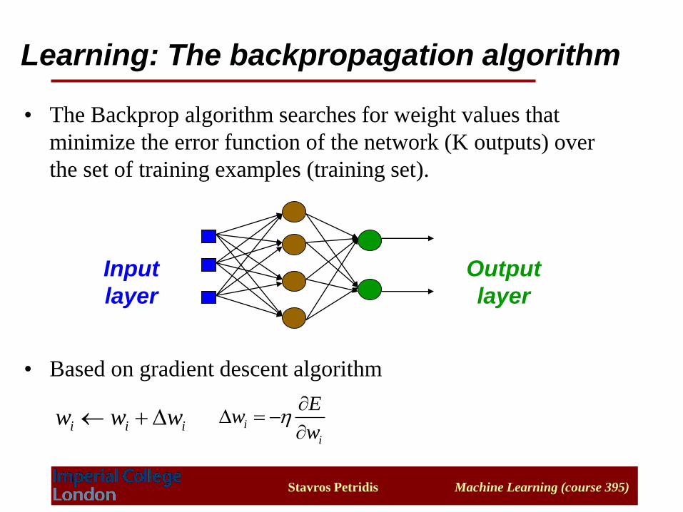
• The Backprop algorithm searches for weight values that
minimize the error function of the network (K outputs) over
the set of training examples (training set).
• Based on gradient descent algorithm
Input
layer
Output
layer
Learning: The backpropagation algorithm
iii www i
iw
Ew
-
Stavros Petridis Machine Learning (course 395)
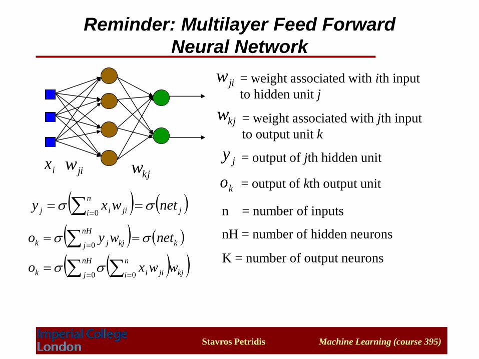
Reminder: Multilayer Feed Forward
Neural Network
jiwkjwix
jiw = weight associated with ith input
to hidden unit j
kjw = weight associated with jth input
to output unit k
jy
ko
= output of jth hidden unit
= output of kth output unit
( ( j
n
i jiij netwxy 0
( ( k
nH
j kjjk netwyo 0
n = number of inputs
nH = number of hidden neurons
K = number of output neurons ( (
nH
j kj
n
i jiik wwxo0 0
Stavros Petridis Machine Learning (course 395)
Backpropagation: Initial Steps
• Training Set: A set of input vectors 𝑥𝑖 , 𝑖 = 1…𝐷with the corresponding targets 𝑡𝑖
• η: learning rate, controls the change rate of the weights
• Begin with random weights (use one of the initialisation
strategies discussed later)
Stavros Petridis Machine Learning (course 395)
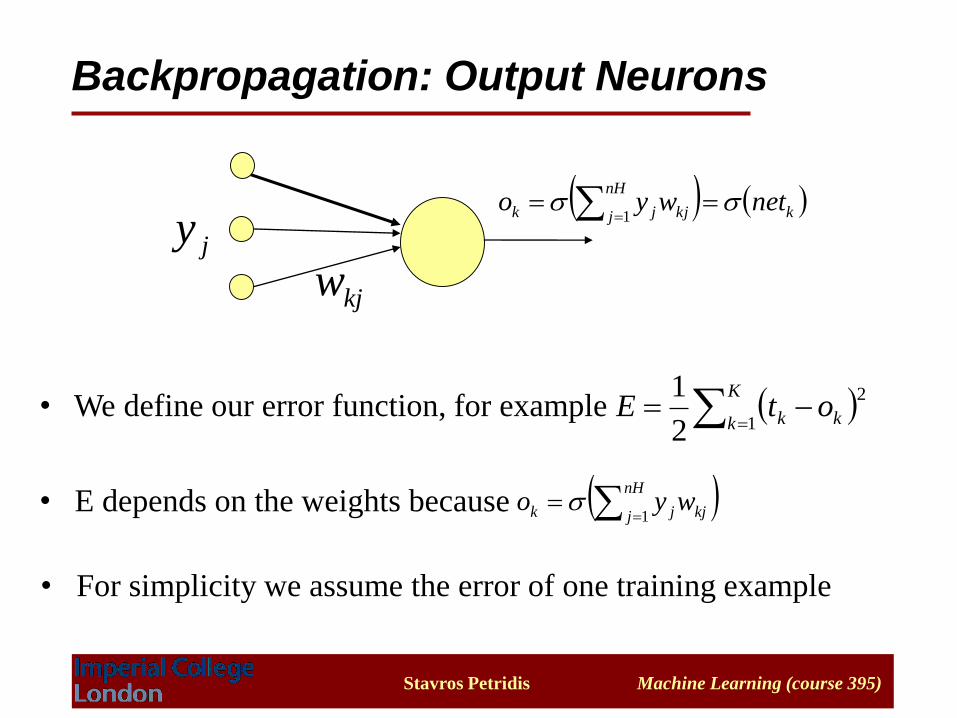
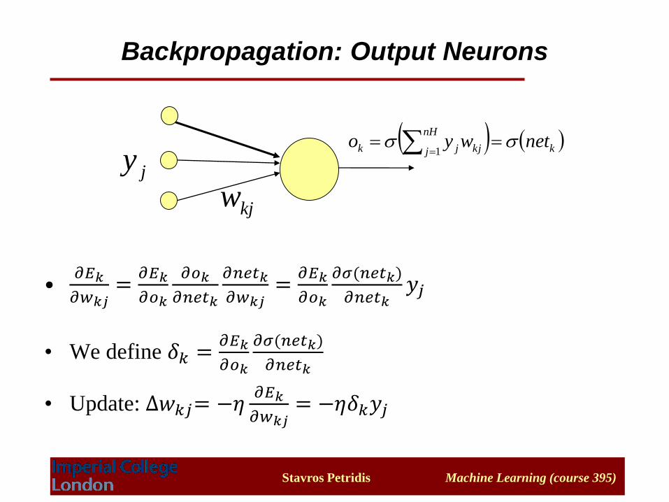
Backpropagation: Output Neurons
• We define our error function, for example
• E depends on the weights because
jy
kjw
( ( k
nH
j kjjk netwyo 1
( -
K
k kk otE1
2
2
1
• For simplicity we assume the error of one training example
(
nH
j kjjk wyo1
Stavros Petridis Machine Learning (course 395)
•𝜕𝐸𝑘
𝜕𝑤𝑘𝑗=
𝜕𝐸𝑘
𝜕𝑜𝑘
𝜕𝑜𝑘
𝜕𝑛𝑒𝑡𝑘
𝜕𝑛𝑒𝑡𝑘
𝜕𝑤𝑘𝑗=
𝜕𝐸𝑘
𝜕𝑜𝑘
𝜕𝜎(𝑛𝑒𝑡𝑘)
𝜕𝑛𝑒𝑡𝑘𝑦𝑗
• We define 𝛿𝑘 =𝜕𝐸𝑘
𝜕𝑜𝑘
𝜕𝜎(𝑛𝑒𝑡𝑘)
𝜕𝑛𝑒𝑡𝑘
• Update: ∆𝑤𝑘𝑗= −𝜂𝜕𝐸𝑘
𝜕𝑤𝑘𝑗= −𝜂𝛿𝑘𝑦𝑗
Backpropagation: Output Neurons
jy
kjw
( ( k
nH
j kjjk netwyo 1
Stavros Petridis Machine Learning (course 395)
Input
layer
Output
layer
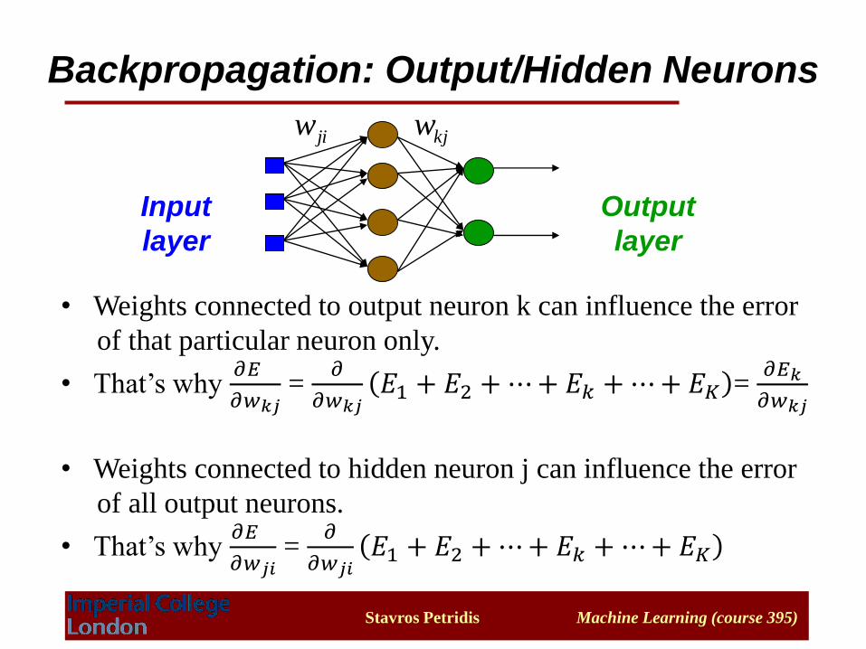
Backpropagation: Output/Hidden Neurons
• Weights connected to output neuron k can influence the error
of that particular neuron only.
• That’s why 𝜕𝐸
𝜕𝑤𝑘𝑗=
𝜕
𝜕𝑤𝑘𝑗𝐸1 + 𝐸2 +⋯+ 𝐸𝑘 +⋯+ 𝐸𝐾 =
𝜕𝐸𝑘
𝜕𝑤𝑘𝑗
• Weights connected to hidden neuron j can influence the error
of all output neurons.
• That’s why 𝜕𝐸
𝜕𝑤𝑗𝑖=
𝜕
𝜕𝑤𝑗𝑖𝐸1 + 𝐸2 +⋯+ 𝐸𝑘 +⋯+ 𝐸𝐾
jiw kjw
Stavros Petridis Machine Learning (course 395)
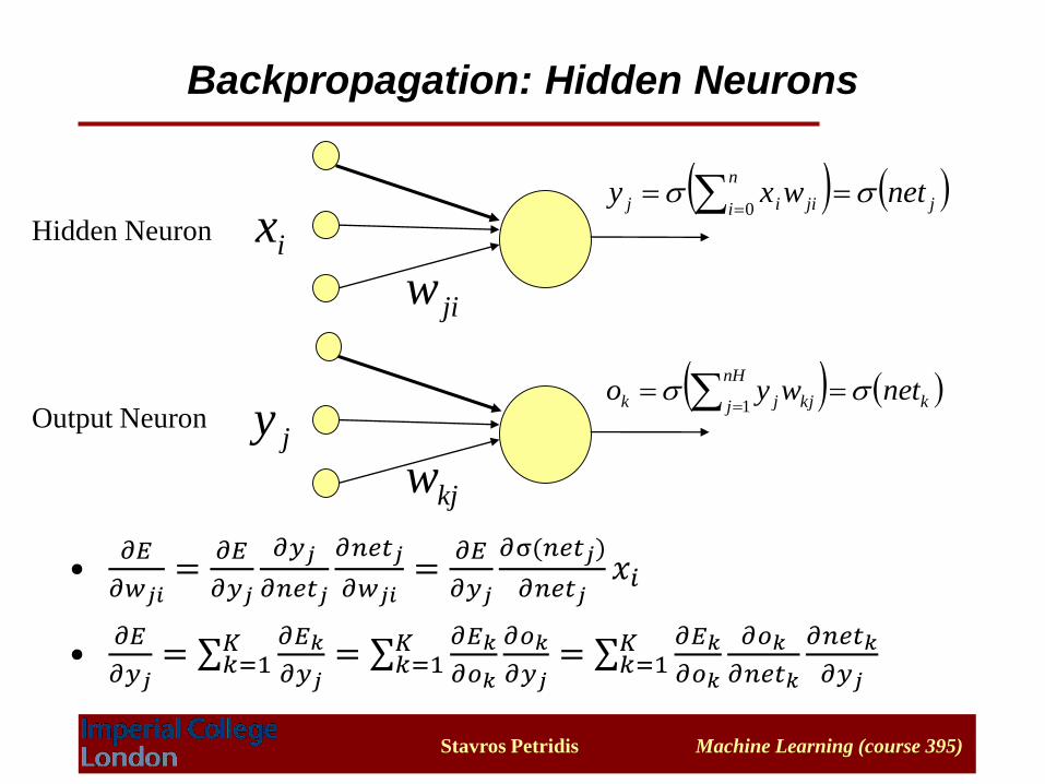
•𝜕𝐸
𝜕𝑤𝑗𝑖=
𝜕𝐸
𝜕𝑦𝑗
𝜕𝑦𝑗
𝜕𝑛𝑒𝑡𝑗
𝜕𝑛𝑒𝑡𝑗
𝜕𝑤𝑗𝑖=
𝜕𝐸
𝜕𝑦𝑗
𝜕σ(𝑛𝑒𝑡𝑗)
𝜕𝑛𝑒𝑡𝑗𝑥𝑖
•𝜕𝐸
𝜕𝑦𝑗= σ𝑘=1
𝐾 𝜕𝐸𝑘
𝜕𝑦𝑗= σ𝑘=1
𝐾 𝜕𝐸𝑘
𝜕𝑜𝑘
𝜕𝑜𝑘
𝜕𝑦𝑗= σ𝑘=1
𝐾 𝜕𝐸𝑘
𝜕𝑜𝑘
𝜕𝑜𝑘
𝜕𝑛𝑒𝑡𝑘
𝜕𝑛𝑒𝑡𝑘
𝜕𝑦𝑗
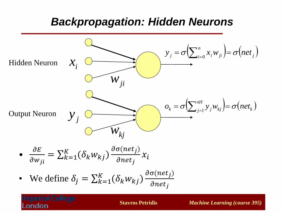
Backpropagation: Hidden Neurons
ix
jiw
( ( j
n
i jiij netwxy 0
jy
kjw
( ( k
nH
j kjjk netwyo 1
Hidden Neuron
Output Neuron
Stavros Petridis Machine Learning (course 395)
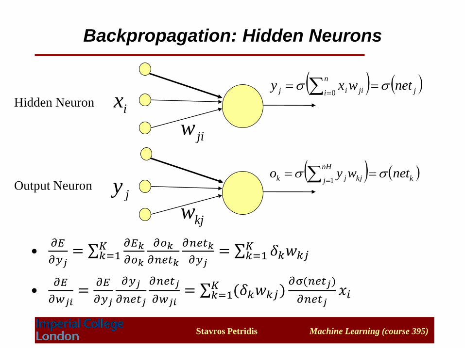
•𝜕𝐸
𝜕𝑦𝑗= σ𝑘=1
𝐾 𝜕𝐸𝑘
𝜕𝑜𝑘
𝜕𝑜𝑘
𝜕𝑛𝑒𝑡𝑘
𝜕𝑛𝑒𝑡𝑘
𝜕𝑦𝑗= σ𝑘=1
𝐾 𝛿𝑘𝑤𝑘𝑗
•𝜕𝐸
𝜕𝑤𝑗𝑖=
𝜕𝐸
𝜕𝑦𝑗
𝜕𝑦𝑗
𝜕𝑛𝑒𝑡𝑗
𝜕𝑛𝑒𝑡𝑗
𝜕𝑤𝑗𝑖= σ𝑘=1
𝐾 (𝛿𝑘𝑤𝑘𝑗)𝜕σ(𝑛𝑒𝑡𝑗)
𝜕𝑛𝑒𝑡𝑗𝑥𝑖
Backpropagation: Hidden Neurons
ix
jiw
( ( j
n
i jiij netwxy 0
jy
kjw
( ( k
nH
j kjjk netwyo 1
Hidden Neuron
Output Neuron
Stavros Petridis Machine Learning (course 395)
•𝜕𝐸
𝜕𝑤𝑗𝑖= σ𝑘=1
𝐾 (𝛿𝑘𝑤𝑘𝑗)𝜕σ(𝑛𝑒𝑡𝑗)
𝜕𝑛𝑒𝑡𝑗𝑥𝑖
• We define 𝛿𝑗 = σ𝑘=1𝐾 (𝛿𝑘𝑤𝑘𝑗)
𝜕σ(𝑛𝑒𝑡𝑗)
𝜕𝑛𝑒𝑡𝑗
Backpropagation: Hidden Neurons
ix
jiw
( ( j
n
i jiij netwxy 0
jy
kjw
( ( k
nH
j kjjk netwyo 1
Hidden Neuron
Output Neuron
Stavros Petridis Machine Learning (course 395)
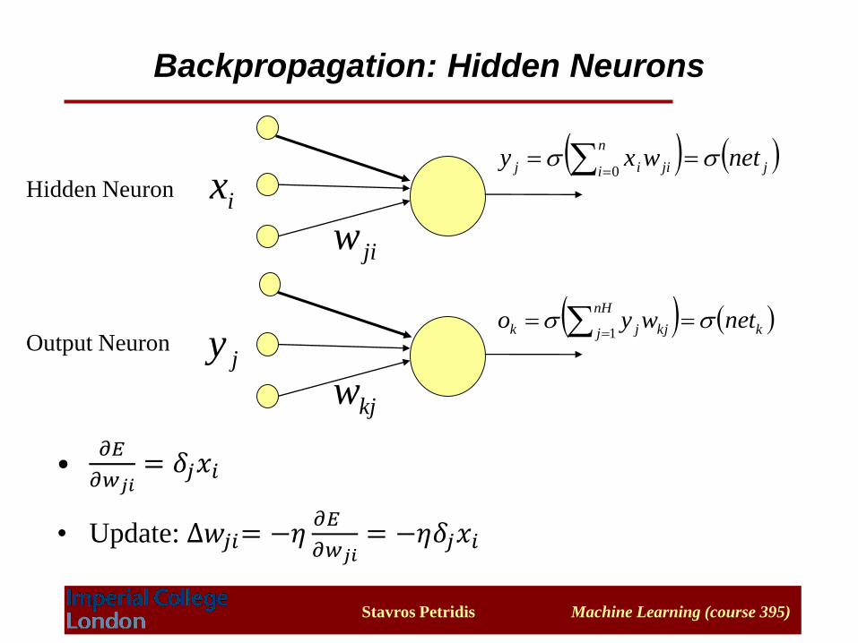
•𝜕𝐸
𝜕𝑤𝑗𝑖= 𝛿𝑗𝑥𝑖
• Update: ∆𝑤𝑗𝑖= −𝜂𝜕𝐸
𝜕𝑤𝑗𝑖= −𝜂𝛿𝑗𝑥𝑖
Backpropagation: Hidden Neurons
ix
jiw
( ( j
n
i jiij netwxy 0
jy
kjw
( ( k
nH
j kjjk netwyo 1
Hidden Neuron
Output Neuron
Stavros Petridis Machine Learning (course 395)
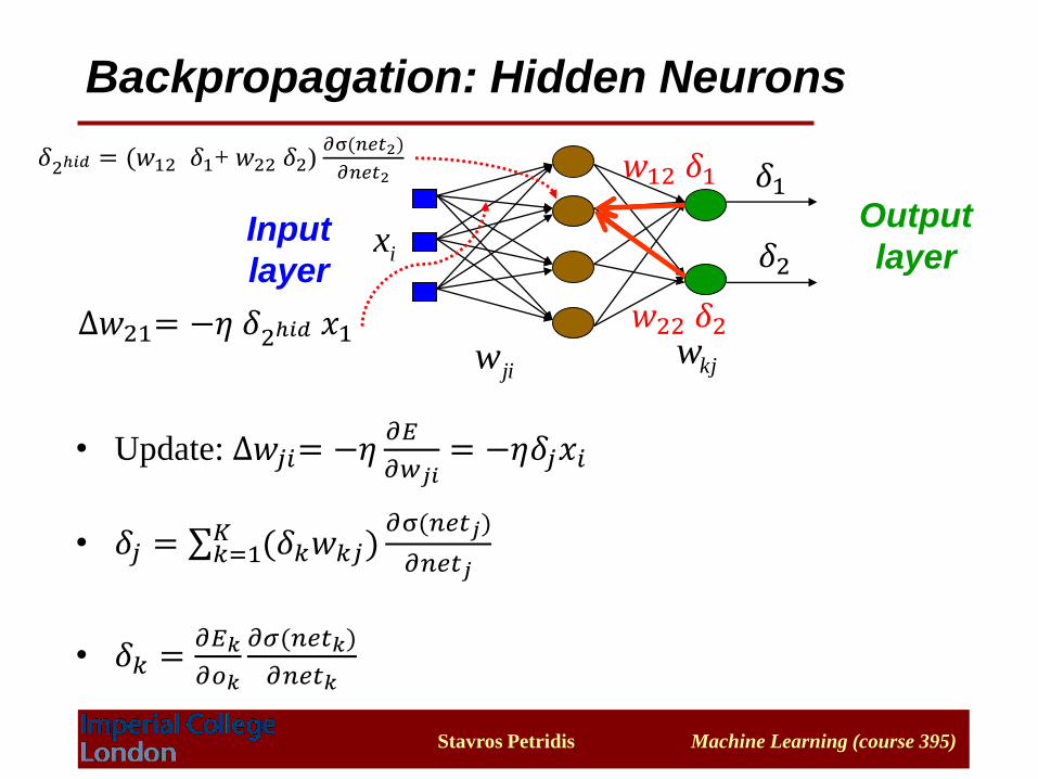
Input
layer
Output
layer
Backpropagation: Hidden Neurons
• Update: ∆𝑤𝑗𝑖= −𝜂𝜕𝐸
𝜕𝑤𝑗𝑖= −𝜂𝛿𝑗𝑥𝑖
• 𝛿𝑗 = σ𝑘=1𝐾 (𝛿𝑘𝑤𝑘𝑗)
𝜕σ(𝑛𝑒𝑡𝑗)
𝜕𝑛𝑒𝑡𝑗
• 𝛿𝑘 =𝜕𝐸𝑘
𝜕𝑜𝑘
𝜕𝜎(𝑛𝑒𝑡𝑘)
𝜕𝑛𝑒𝑡𝑘
jiw kjw
ix
𝛿1
𝛿2
𝑤12 𝛿1
𝑤22 𝛿2
𝛿2ℎ𝑖𝑑 = (𝑤12 𝛿1+ 𝑤22 𝛿2)𝜕σ(𝑛𝑒𝑡2)
𝜕𝑛𝑒𝑡2
∆𝑤21= −𝜂 𝛿2ℎ𝑖𝑑 𝑥1

Stavros Petridis Machine Learning (course 395)
Example
• http://galaxy.agh.edu.pl/~vlsi/AI/backp_t_en/backprop.html