MASTERS THESIS

Coupling Game Theory and Discrete-EventSimulation for Model-Based Ambulance

Dispatching

Author:XinYu FU

Daily Supervisor:dr. Sergey V. KOVALCHUK

Examiner:dr. Valeria KRZHIZHANOVSKAYA

Assessor:dr. Michael LEES

A thesis submitted in fulfillment of the requirementsfor the degree of Master of Science in Computational Science

in the

University of Amsterdam ITMO University

July, 2020

ABSTRACT

Patients in critical medical conditions need professional facilities, and usually, the diseaseoccurs in an unexpected situation, therefore properly allocating medical resources becomes es-sential for them. Particularly, for acute coronary syndrome (ACS) patients in the metropolitanareas of Saint Petersburg, Russia, overcrowding is caused by the irregular inflow of patientsand the limited resources of angiographies (a medical imaging technique requires profession-als and equipment). An applied solution is that overcrowded hospitals (or emergency depart-ments, ED) can divert incoming patients to other hospitals. During the redirecting process,stakeholders such as hospitals, patients, ambulance squad, emergency medical service (EMS)and city authorities are involved. Thus, decisions on the collaborative management of pa-tient flow form a non-cooperative game (a game with competition between individual players)which is incentivised by stakeholders’ self-enforcing operations. Consequently, the social opti-mum of health outcome is hardly achieved. Thus, the demand for investigating the behavioursof stakeholders is emerging.

Because of the complex interactions among stakeholders and global regulation mixed withlocal decision-making, the behaviour pattern of stakeholders is complicated. Moreover, thecomplexity is increasing because the level of patients inflow is irregular; the real-time trafficcondition is affecting the delivery time; the hospitals’ strategies are dynamic. To consider theabove factors, we suppose there are global mechanisms of regulation: 1. Queuing theory isguiding the process of patient inflow 2. self-enforcing operation derived from game theory areguiding the hospital’s actions. As a result, the mechanisms are influential to the social metricof health outcome (e.g. global mortality).

In general, the research sets up a GT-DES model coupling the game theory(GT) and dis-crete event simulation(DES) for analysing the behaviours of patients and hospitals.The sim-ulation assumes hospital acts for the sake of a balance between its own lower mortality andmore patients being served. The model can be used to demonstrate the process of patient in-flows, reveal the predictive strategies of hospital individuals and to find Nash equilibrium.Notably, based on the real data and consultation from medical professionals in Saint Peters-burg, a real-world case about modelling ambulance dispatching of ACS patients by GT-DESmodel is studied. The datasets contain the information of eleven 24-7 hospitals located in SaintPetersburg, 5124 ACS records, 1866 records of serving time to stent patients during ten monthsand 1,310,263 node-to-node travelling paths in Saint Petersburg.

Technically, we firstly deployed a mathematical queuing-network model (QNM) for a

one-dimensional scenario with two hospitals. Secondly, we integrated the stochastic ueuing-network model and game-theoretical approach to a GT-DES model for a two-dimensional sce-nario. In which, a sensitivity analysis (Sobol Indices) is performed to explore the importanceof the factors. Lastly, a case about simulating the ambulance dispatching of ACS patients inSaint Petersburg is studied based on the real data. In which, a connection between the mortal-ity and door-to-balloon time is constructed for mortality estimation. In addition, the model isvalidated by the comparative analysis of the simulated mortality and observed mortality usingPearson correlation test. Also, the result among 130 possible strategy combinations shows, thestrategy combination predicted by GT-DES model has the highest correlation to the observedmortality.

In conclusion, the decision-making process of hospitals is mainly influenced by the levelof patient inflow and the amount of medical resource owned by itself and nearby hospitals.As a result of interactions among all hospital agents, a Nash equilibrium can be formed, andit is possible to be predicted by the game-theoretical model. Lastly, the case studied showsa practical significance in modelling ambulance dispatching for specific patients and can beextended and applied to other city environments.

0

CONTENTS

Abstract

1 Introduction 21.1 Research question . . . . . . . . . . . . . . . . . . . . . . . . . . . . . . . . . . . . . 21.2 Methodology . . . . . . . . . . . . . . . . . . . . . . . . . . . . . . . . . . . . . . . 31.3 Research contributions . . . . . . . . . . . . . . . . . . . . . . . . . . . . . . . . . . 41.4 Thesis outline . . . . . . . . . . . . . . . . . . . . . . . . . . . . . . . . . . . . . . . 4

2 Literature Review 62.1 Modelling simulation for emergency medical service operations . . . . . . . . . . 62.2 Discrete event simulation . . . . . . . . . . . . . . . . . . . . . . . . . . . . . . . . 72.3 Game theory for ambulance dispatching . . . . . . . . . . . . . . . . . . . . . . . . 9

3 Methods and Model Development 113.1 Conceptual model . . . . . . . . . . . . . . . . . . . . . . . . . . . . . . . . . . . . . 113.2 One-dimensional analytical queuing-network model (QNM) . . . . . . . . . . . . 133.3 Two-dimensional stochastic GT-DES model . . . . . . . . . . . . . . . . . . . . . . 173.4 Implementation details . . . . . . . . . . . . . . . . . . . . . . . . . . . . . . . . . . 213.5 Scenario design . . . . . . . . . . . . . . . . . . . . . . . . . . . . . . . . . . . . . . 223.6 Sensitivity analysis by the Sobol method . . . . . . . . . . . . . . . . . . . . . . . . 26

4 Experimental Study and Results 304.1 Simulating with artificial settings . . . . . . . . . . . . . . . . . . . . . . . . . . . . 30

4.1.1 Warm-up simulation . . . . . . . . . . . . . . . . . . . . . . . . . . . . . . . 304.1.2 Result of GT-DES model with multiple hospitals . . . . . . . . . . . . . . . 33

4.2 Simulating ambulance dispatching of ACS patients in Saint Petersburg . . . . . . 394.2.1 Background . . . . . . . . . . . . . . . . . . . . . . . . . . . . . . . . . . . . 394.2.2 Data description . . . . . . . . . . . . . . . . . . . . . . . . . . . . . . . . . 404.2.3 Scenarios . . . . . . . . . . . . . . . . . . . . . . . . . . . . . . . . . . . . . . 414.2.4 Simulation Results . . . . . . . . . . . . . . . . . . . . . . . . . . . . . . . . 41

1

Modelling ACS patients in Saint Petersburg . . . . . . . . . . . . . . . . . 41Local simulation with isolated hospitals . . . . . . . . . . . . . . . . . . . . 49Global simulation with all hospitals in Saint Petersburg . . . . . . . . . . . 49

4.3 Interpretation, discussion and validation . . . . . . . . . . . . . . . . . . . . . . . 52

5 Conclusion and Future Work 585.1 Conclusion . . . . . . . . . . . . . . . . . . . . . . . . . . . . . . . . . . . . . . . . . 585.2 Possible futurework . . . . . . . . . . . . . . . . . . . . . . . . . . . . . . . . . . . . 59

A Supplementary Results 61A.1 Probability of Nash equilibrium for all hospital pairs . . . . . . . . . . . . . . . . 61

List of Figures 63

List of Tables 67

Reference 69

2

1 INTRODUCTION

Recent evidence [36] suggests that an of particular concern in the health-care system isimbalance: some hospitals are always overcrowded while the others are preferably free. Forinstance, according to our data about 13 hospitals in Saint Petersburg, the northern region ofthe city has less density of inhabitants but more hospitals compared with the southern part.It may happen, when the hospitals in the south are in full load, the hospitals in the northare working cosily. Typical reasons can be the increasing number of visits to the emergencydepartment (ED) and decreasing facilities in ED [30]. As a result, the imbalanced allocation ofmedical resources may lead to economic waste, health waste and loss of public trust.

Generally, the simplest solution to overcrowding is to increase the capacity of the resource.However, R.A. McCain’s study [28] proposed a verified Nash equilibrium hypothesis for over-crowding issue, and they suggested that increasing ED capacity has a fewer impact. Thus, apractical solution is that EMS distributes patients to hospitals reasonably from a global per-spective. Another solution is to allow redirecting the ambulance fleet by the hospital receiver.For instance, overcrowded hospitals can redirect patients’ requests, so that EMS can arrangethe patients to another preferably free hospital. Theoretically, all the hospitals in the system canshare the loads properly [8]. However, some evidence shows that social optimum may not beachieved in this decentralised ambulance-dispatching system due to incentives of stakeholders(i.e. hospitals, patients, ambulance squad, emergency medical service (EMS) and city author-ities) [8]. Thus, the demand for investigating the behaviours of stakeholders in a ambulance-dispatching system is emerging.

1.1 Research question

The ambulance dispatching system (ADS) is a system that helps optimise the medical re-source allocation by properly scheduling urgent patients to a medical facility [3]. In which,emergency medical services (EMS) operates as the coordinator to answer an emergency calland assign an ambulance fleet to the emergency site, and transport patient to a medical facil-ity if the patient requires. Emergency department (ED) is a typical medical facility providing

3

acute care to scheduled patients from emergency medical service which is usually attached toa hospital and medical centre.

The ambulance-dispatching system can be categorised into two groups: centralised anddecentralised network. A centralised ambulance-dispatching system suppose scheduling andredirecting the incoming patients are dominantly guided by emergency medical services (EMS),in which EMS functions as a centre to assign the proper ED to incoming ambulance fleets. Inrealistic, ambulance-dispatching systems in many cities are decentralised, in which the EMSworks as a message-passing agent.

An underlying problem is whether the hospitals are willing to sacrifice their interests (be-cause redirecting incoming patients usually results in patient lost). Consequently, system per-formance may not be optimised. For instance, a recent paper [8] claimed the same situationand found a Nash equilibrium among EDs. Also, [29] mentioned that in West San FernandoValley, hospitals lose money when profitable ambulances turned away. In other words, medi-cal facilities use defensive equilibrium to protect themselves from turning incoming ambulanceto other medical facilities. Likewise, we have seen functional similarities in dispatching acutecoronary syndrome (ACS) patients in Saint Petersburg. The specialist explains that when ahospital receives a request from the emergency medical service (EMS), the hospital will acceptpatients as much as possible if only the financial profit is considered. However, as a humanistorganisation being responsible to the society, the health outcome of the patient is also vital.Thus the current capacity of medical resources and ability would be taken into account whiledeciding to make sure the patient will have high-quality salvation. It turns out there is a littlecorporation between nearby hospitals so-called as a non-cooperative game in game theory.

The research goals will be the following: (1) to observe and simulate the process of pa-tient inflow such as arrival, travelling and serving process. (2) to predict hospitals’ actionsin a non-cooperative game by Nash equilibrium, and to dig out the transition pattern ofpredicted actions. (2) to reason the factor importance resulting in the hospital’s action tran-sition. (3) to study the practical use of the GT-DES model by applying it to a real-worldcase.

1.2 Methodology

In the thesis, we will propose a game theoretical(GT)-discrete event simulation (DES)model. In this paper, an analytical and stochastic queuing-network model (QNM) princi-pally based on DES are firstly deployed for modelling arrival, travel and serving process ofpatients[4] [22]. What is more, a game-theoretical approach is constructed to predict hospitalactions by searching for the pure Nash equilibrium.

4

The proposed GT-DES model is set up as a universal framework, meaning we put moreeffort to make the model more simple, general and extendable. At the same time, many exper-iment feasibility and possible scenarios in realistic will be discussed and reasoned. Althoughthe prototype of our model is based on the health-care system in Saint Petersburg, Russia, webelieve it could be modified to adapt to a new health-care environment with less effort.

1.3 Research contributions

Two main contributions from the thesis are

1. A generalised model coupling game theory and discrete event simulation (GT-DES) tomodel decentralised ambulance-dispatching system.

2. A case study about modelling the ambulance dispatching of ACS patients in Saint-Petersburg,and predicting hospital strategies with the support of real-world data and consultationfrom medical professionals.

1.4 Thesis outline

FIGURE 1.1: A modelling and simulation life cycle applied to structure a computational model [16]

This thesis gradually explains the model following the model-simulation life cycle as shownin Figure.1.1.

1. System we studied are introduced in Chapter 1, which introduces research backgroundand goals and Chapter 2 which is the relevant literature .

5

2. Conceptual model is introduced in Section 3.1

3. Computational GT-DES model is introduced in section 3.3

4. In simulation, a sensitivity analysis is performed in section 3.6

5. Chapter 4 demonstrates the simulation results and the practical case study

6. Eventually, we come back to the system we studied in Chapter ?? by concluding ourfindings and possible future works.

6

2 LITERATURE REVIEW

This chapter has included related works and literature review gathered while doing theproject.

2.1 Modelling simulation for emergency medical service operations

Over the past ten years, many studies are involved in developing computational mod-els to answer ambulance dispatching questions. A critical element in ambulance dispatchingsystem is emergency medical service (EMS); it is a pre-hospital component conducts activi-ties including screening incoming call for emergency purpose and scheduling transportationof ambulance fleets. Gradually, the trends to EMS problems were transiting from strategical,tactical decision level to operational decision level because of growing computational tech-nology[5]. Recently, considerable operational research (OR) literature illustrated models forshort-term EMS decision problems such as 1) scheduling more than one ambulance fleet to acall to reduce service time. 2) assigning proper medical facilities to patients to reduce the timeconsumption in transportation and medical transmission. 3) switching target medical facilityto another one (which usually is preferably free) as redeployment strategy [18]. This reviewfocuses more on short-term decision problem in OR level research conducted by EMS becausethe project is real-time ambulance relocation which is in this area.

The emergency medical services (EMS) can be classified into two systems: anglo-Americanand franco-German EMS [10]. The simulation method was usually initially developed for oneof the systems. However, it is possible to form typical EMS operations firstly. In which, atypical EMS operations consists of following steps: (1) arrival of an emergency call, (2) callscreening, (3) vehicle dispatching, (4) vehicle travelling from its current location to the emer-gency site, (5) on-site treatment, and (6) patient transportation to a health facility if required[5].

For a computational model, the performance measure is a crucial element for the specificproblems. Time consumption, survival rate and economic costs are the main aspects of perfor-mance measure for an ambulance dispatching system. A typical example of time-consumption

7

measures is using average response time (defined as the duration between the recital of calland the first arrival of ambulance fleet) [17][41]. The survival rate is a straightforward measurefor the death-cause disease. However, it is less used in research due to the difficulty to describeit quantitatively.

[18] proposed three critical characteristics for a successful EMS operations model: the ar-rival distribution, the geographical distribution and the priority of calls. However, geograph-ical distribution varies in different cities and the priority categorisation changes as well. Thearrival distribution can be seen as a result of the Poisson process or extracted from real-worlddata [13]. The geographical distribution has a crucial impact on travelling time. [41] uses a sim-ple mathematical method to compute the distance in time by Euclidean distance. But recentresearches involves data capture technologies such as GPS (global positioning system) for de-tailed routes since traffic conjunction and road complexity are also explained by GPS distance.A defect to be considered is ambulance has high road priority.Other things to be consideredwhile setting up an ADS is delivery efficiency. Because it is critical in reducing mortality anddisability rates [25]. Coverage and response time are two vital factors for valuate delivery ef-ficiency [31]. [25] also suggested that two significant factors to ambulance relocation in theambulance-dispatching system are the fleet size and hospital locations.

In many models, the principle of proximity is used as the main dispatch rule, such as[47] [23]; where patients were sent to the nearest available base for treatment if transportationrequired . The reason is that the principle of proximity is simple and practically used. Yetsometimes, "the nearest base" may not accept patients for reasons such as lacking medicalresource, expected waiting time is too long [12], a redirection or relocation of ambulance fleetwill be conducted by together EMS and the assigned medical facility in a decentralised system.Besides, Cheng Siong Lim’s paper [25] introduced multiple ambulance dispatch policies anddynamic ambulance relocation models from the perspective of dispatch policies. It turns outwith applying dispatch policy, response time to urgent calls is reduced.

2.2 Discrete event simulation

One method for quantitatively conducting input–throughput–output analyses for patientflows in ED is through detailed computer simulation[6] In practice, techniques such as decisionanalysis, Markov process, mathematical modelling, system dynamics, agent-based modelling(ABM) and discrete event simulation (DES) have all been applied in modelling the heath-caresystem; discrete event simulation (DES) and agent-based modelling (ABM) are the most com-monly used techniques for modelling patient flow and interactions between players. Discreteevent simulation (DES) is a technique for modelling a system that can change at a point in

8

time. The agent-based model (ABM) simulates the interactions between agents where agentsare evaluated as a combination of attributes and entities. The main difference between themis the level of perspective. DES is an event-driven simulation, but ABM focuses more on in-teractions between agents. Therefore, normally DES answers questions such as estimating thewaiting time and queuing length, while ABM reveals the pattern after agents interact with eachother.

Discrete event simulation (DES) has been developed to allow modelling of discontinuoussystems by defining activity as a network of interdependent discrete events [35] The analyticalmethods do not solve the discrete events, but using a computer program to run the modelby generating random numbers (e.g. by Monte Carlo method) as numerical methods. Thesimulation of the system arises from the assumptions of the model, and the researchers collectand observe operational data to analyse and estimate the performance of the real system [4].

DES is now widely applied in various fields. It is used in production, logistics, militaryand other areas, and has played a decision-support role. In the area of modelling the health-care system, discrete event simulation has its unique advantages. Firstly, DES integrates therandom factors in the operation of the ED and patients. The processes of the model can reflectthe running state of the ED and the patient flow, and provide the critical system performancewith related data, such as staying time, waiting time of patients, the capacity of resources inED, and its utilisation. The construction of the DES model can also deepen the understand-ing of the health-care system. Running simulation experiments can virtually change the ED’sstructure or inputs without changing the actual operating conditions of the ED.’ For this reasondiscrete event simulation is a popular and useful decision-making tool in the field of modellinga health-care system in recent years. Furthermore, the simulation results can be widely used inpractice, such as reducing the cost of medical services and helping to improve patients satisfac-tion. An example for modelling emergency medical services and emergency departments thatSun Xu [43] suggested is a queuing model (principally based on discrete event simulation) sim-ulate the emergency-care delivery system. A continuous-time Markov chain is acquainted forthe network model. Besides, LG Connelly and AE Bair [6] proposed a system platform namedEmergency Department SIMulation (EDSIM), a newly developed DES model of ED activity inan academic Level 1 trauma centre. The research novelty is EDSIM is that DES-based simula-tion primarily concentrates on "patient path" in ED. The patient path is defined as a series ofindividual activity which has to be to completed before discharge. EDSIM simulates continu-ally queuing jobs with prioritisation. With the help of the understanding of staffing levels, fa-cility characteristics and patient data drawn from electronic patient tracking databases, billingrecords. The model predicts average patient service times within 10% of actual values. Anadditional scenario that should be carefully examined and simulated in DES is overcrowding.

9

When in overcrowding, an ED can request the emergency medical services (EMS) agency todivert incoming ambulances to neighbouring hospitals, a phenomenon known as "ambulancediversion." [8] However, A non-negligible issue to consider is when and in what condition theED should divert patient to other EDs. Sarang Deo and colleagues propose a possible solutionto this problem; they decided the redirecting threshold by the sum of the capability of ED andaverage patients queuing in ED if there is a vacancy in ED. So that the policy could pool theresources of many ED. Not only it optimises the benefits and easily practicable, but also it isproven to be a Pareto improvement.

2.3 Game theory for ambulance dispatching

Game theory, a concept founded in 1944, is an analytical method for the actions of play-ers in an interactive situation [32]. Game theory is a theory based on assumptions of rationalchoice and focusing on interactive decision making—has the potential to provide models ofthe consultation that can be used to generate empirically testable predictions about the factorsthat promote quality of care [44]. Game theory provides a supplementary means to expli-cate optimal rational strategies in situations where the actual outcome depends on the choicesof the ED[9]. A game-theoretical analysis is usually performed using rigorous mathematicalmodels to consider the optimal decision-making problem under certain conflicting conditions.Nowadays, game theory is frequently applied to in-depth analysis under various social andeconomic options, as well as a health-care system. And it has obtained fruitful research resultsin multiple disciplinary fields [1] [48].

As an analytical tool, game theory is used to help people observe and understand theinteractions and relationship between players. As a method and technology to guide the for-mulation of health-care policies, the game-theoretical model mainly analyses the policy envi-ronment through game theory and predicts and explains the behaviours of policy recipients,city authorisations and related organisations.

When formulating a heath-care plan such as an ambulance-dispatching rule, the city au-thority must consider its own sake (social optimal), as well as the purpose of the relevantrecipients. The sake usually consists of economic and social benefits. Game theory provides away to demonstrate the final-interest balance among players.

The games can be categorised into two groups: cooperative game and non-cooperativegames. It is commonly assumed that modelling the centralised system as a cooperative gameand decentralised system as a non-cooperative game [26]. Ideally, non-cooperative games onlyhave competition. And most of the policies in the non-cooperative game can optimise thescheme by seeking the Nash equilibrium solution of the policy game [46]. [8] founded the

10

ambulance diversion has defensive equilibrium as a non-cooperative-game system. Wherererouting patients could not reach social optimum because ED aims to minimise their ownwaiting time instead of global waiting time. In the proposed GT-DES model, we model thedecentralised ambulance dispatching system as a non-cooperative game.

As a comparison, cooperative-game ADS suggests that the EMS is the only rule-maker andcan arrange the diversions of the ambulance on behalf of the efficiency of the system [8]. Thereare two advantages compared with decentralised ambulance diversion; one is that the systemwill have less chance to reach defensive equilibrium. What is more, the waiting time is indeedreduced. By considering the distance between ED, we can optimise the global time. Likewise,the system reached Pareto improvement. Extensive research has shown that the game theorymodel is a feasible way to simulate the cooperative actions of the player. R. Hagtvedt et al.[14] provided new insights by proposing a cooperative game to reduce ambulance diversion,which is a bit more complicated. Hardy and Te [11] examined this idea in his work at DeKalbMedical Centre (DKMC) in Atlanta, GA. The two types of games can be transformed into eachother under certain conditions, such as maximising the pursuit of own interests.

11

3 METHODS AND MODEL DEVELOPMENT

In this section, the model development and methods will be explained. Firstly, the GT-DESmodel will be discussed both conceptually and computationally. The GT-DES model containstwo sub-models that are simulated separately 1. a queuing network model (QNM, principallymodelled as discrete event simulation) to simulate patients’ arrival(including requesting andtravelling process) and serving process. 2. a game-theoretical model to predict the defensiveactions ("Accepting" or "Redirecting") of hospitals. Also, a situation where patients are uni-formly distributed in the city is configured for the artificial simulation. In addition, a sensitivityanalysis by Sobol method is performed to understand the factor importance.

3.1 Conceptual model

This section reveals the conceptual process of the GT-DES model. There are three mainroles in an ambulance-dispatching system:

1. The patient is the main consumer to emergency medical service (EMS) and needed tobe served in a hospital. During the simulation, We focus on a type of patients who areobligatory to be transferred to ED, meaning patients could not be cured by First Aid suchas acute coronary syndrome (ACS) patients.

2. Emergency department (ED) or hospital (because ED is usually attached to a hospital) is amedical facility to serve incoming patients. In this thesis, ED and hospital are categorizedas the same type of medical facility and will be used as the same agent. Conceptually, EDis an accurate term focusing on serving the patients in emergence. However, walk-inpatients to hospitals and other types or surgery-wanted patients may also be consideredin the model. In the proposed GT-DES model, two main interests for ED or hospital areassumed 1. ensuring the quality of patient life. 2. considering serving more patients byED itself. Thus, ED or hospital has the incentive to choose if accept or redirect incomingpatients.

3. EMS: emergency medical service is a medical centre where it responses to the incomingemergency call and arranges ambulance squad to help and fetch patients. EMS is also

12

FIGURE 3.1: A flowchart explicitly explains the workflow of the ambulance-dispatching system (ADS)from the perspectives of stakeholders, including patients, emergency medical service (EMS) and ED(or hospital). The whole flowchart will be modelled by queuing-network model analytically andstochastically except the marked comment box will be modelled by the game-theoretical model (GTM)

to predict the strategies of EDs or hospitals.

responsible for sending the patient’s request to a nearby medical facility such as ED,asking for acceptance if a patient needs to be transferred for further aids. Besides, EMSusually collect medical data for the support of policymaker. For instance, our data isprovided by Almazov National Medical Research Centre with the help of EMS in SaintPetersburg, Russia.

The flowchart shown in Figure.3.1 conceptually describes the process of the ambulance-dispatching system from different perspectives. The general process simulated is the following:

13

once patients are fetched by the ambulance, the nearest ED (target ED) is chosen as a top prior-ity. The patient will be sent to target ED if the target ED accepts ("Accepting" strategy). How-ever, suppose the target ED’s strategy is redirecting, and the current number of patients hassurpassed the predefined capacity (the sum of the number of the servers and queuing room).In that case, the ambulance then brings them to the next nearest ED. We repeat this process byasking over all the EDs. If all EDs are busy and reject the patient’s requests, then the patientwill be sent to the best ED with the minimum time spent on travelling and predictive serving.It shall be addressed that in an ambulance-dispatching system, the definition of "server" is seenas any medical resource in realistic which is most crucial to patient healing, could be a medicalfacility, professional doctors, nurses and beds.

3.2 One-dimensional analytical queuing-network model (QNM)

An analytical model is a deterministic model employing mathematical solution withoutrandomness. Three reasons for conducting the one-dimensional analytical model are:

1. It provides us with the opportunity to quickly study the behaviours pattern of the system

2. We can verify ideas before running the stochastic model which has more randomness.

3. The analytical model has a lower cost for computational power, we can manipulate pa-rameters freely.

This section is originally derived from my another paper [12].

Figure.3.2 shows the idea of 1-D queuing-network model . In plain words, we firstly as-sign k = 2 hospitals (denoted as H1 and H2) to each side of the one-dimensional map (Note,we use notation "hospital" instead of "ED" in the computational model). Each hospital has astrategy of “Accepting” (abbr. A, accepting all the patients’ requests) or “Redirecting” (abbr. R,redirecting/diverting patients to opposite hospital if the current number of patients in hospitalexceeds the limited capacity including serving facility and waiting room or queuing buffer).

The process of 1-D model is the following: firstly, the patient is initialised uniformly be-tween H1 and H2 as pi. Next, if the hospital accepts the patient, the patient will be deliveredto a hospital by the principle of proximity. Otherwise, the patient will be redirected to anothernearest hospital. Whenever patients arrived at any hospital, they will be served immediately ifthe hospital has free servers (the term "server" is derived from queuing theory [4]). Otherwise,the patient will be queuing in a waiting room. The serving process follows the principles of"First In First Out" (FIFO) and "First Come First Served".

14

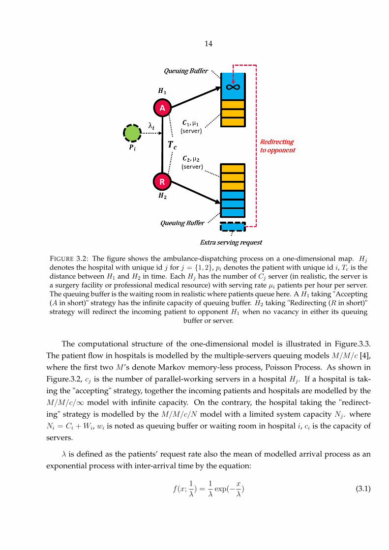
FIGURE 3.2: The figure shows the ambulance-dispatching process on a one-dimensional map. Hj

denotes the hospital with unique id j for j = 1, 2, pi denotes the patient with unique id i, Tc is thedistance between H1 and H2 in time. Each Hj has the number of Cj server (in realistic, the server isa surgery facility or professional medical resource) with serving rate µi patients per hour per server.The queuing buffer is the waiting room in realistic where patients queue here. AH1 taking "Accepting(A in short)" strategy has the infinite capacity of queuing buffer. H2 taking "Redirecting (R in short)"strategy will redirect the incoming patient to opponent H1 when no vacancy in either its queuing

buffer or server.

The computational structure of the one-dimensional model is illustrated in Figure.3.3.The patient flow in hospitals is modelled by the multiple-servers queuing models M/M/c [4],where the first two M ’s denote Markov memory-less process, Poisson Process. As shown inFigure.3.2, cj is the number of parallel-working servers in a hospital Hj . If a hospital is tak-ing the "accepting" strategy, together the incoming patients and hospitals are modelled by theM/M/c/∞ model with infinite capacity. On the contrary, the hospital taking the "redirect-ing" strategy is modelled by the M/M/c/N model with a limited system capacity Nj . whereNi = Ci +Wi, wi is noted as queuing buffer or waiting room in hospital i, ci is the capacity ofservers.

λ is defined as the patients’ request rate also the mean of modelled arrival process as anexponential process with inter-arrival time by the equation:

f(x;1

λ) =

1

λexp(−x

λ) (3.1)

15

FIGURE 3.3: The computational structure of a 1-D queuing-network model (QNM)

Also, M is defined as global serving rate, whilst µ is serving rate of one server with µ =1

Tserving. Thus, we have M = cµ where 1/µ is the mean for the probability density function of

Poisson distribution for serving process:

f(k;1

µ) =

e−1µ

µkk!(3.2)

where 1µ= Tserving is the average serving time and also the mean of Poisson process. There-

fore, the total time of patient pi contains transportation time, queuing time and serving time asthe following:

T itotal = T itravelling + T iqueuing + T iserving (3.3)

Suppose each hospital can select one strategy aj with j being hospital id. Two hospitals in1D map have a1, a2 as strategy combination where a1 ∈ A,R and a2 ∈ A,R (meaning H1

is taking a1 strategy, same a2 to H2). And aj is either accepting strategy or redirecting strategy,the total norm for 1d model are AR/RR/RA/AA situation. Also, we define the load parameterof single server is a = λ/µ and load parameter with multiple servers ρ = λ/cµ.

• In the case of AA (H1 and H2 have Accepting strategy):The request rate in Hj is λj = λ

2, where j ∈ 1, 2 in 1d model.

• In the case of RA (H1 has redirecting strategy and H2 has accepting strategy):Due to the impact of the hospital taking the "redirecting" strategy, we firstly introduce the

16

probability of no patients in the system [4]:

P0 = [1 +c∑

n=1

an/n! + ac/c!N∑

n=c+1

ρn − c]−1

Then we expand it to the probability of N (the capacity of system ) patients in the system,which is equivalent to the probability of redirecting patients prej in the system:

PN = ρnP0

Prej = Pmax =aN

c!cN−cP0

Next, in RA case , the effective λe1 in H1 is [21]:

λe1 = λ1(1− Prej(λ1))

The effective λe2 in H2 is:λe2 = λ2 + λ1Prej(λ1)

• AR case has same result to the case of RA with swapped hospital number i.

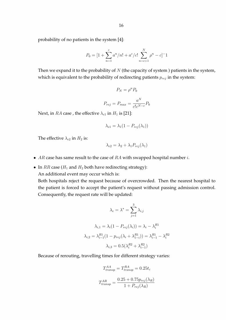
• In RR case (H1 and H2 both have redirecting strategy):An additional event may occur which is:Both hospitals reject the request because of overcrowded. Then the nearest hospital tothe patient is forced to accept the patient’s request without passing admission control.Consequently, the request rate will be updated:

λe = λ∗ =3∑j=1

λi,j

λi,1 = λi(1− Prej(λi)) = λi − λR1i

λi,2 = λR1i−1(1− prej(λi + λR1

1−i)) = λR1i−1 − λR2

i

λi,3 = 0.5(λR2i + λR2

i−1)

Because of rerouting, travelling times for different strategy varies:

TAAtransp = TRAtransp = 0.25tc

TARtransp =0.25 + 0.75prej(λR)

1 + Prej(λR)

17

TRRtransp =0.25λi,1 + 0.75λi,2 + 0.5λi,3

λ∗itc

where Tc is defined as the distance between two hospitals measured by time.

Next, we could deduce some important metrics of the system from a long-term perspec-tive.

Metric 1. The average number of patients in queue and average time of each patient spentin queue [4]:

LQ =P0a

cρ

c!(1− ρ)2)[1− ρN−c − (N − c)ρN−c(1− ρ)]

WQ = LQ/λe

Metric 2. The average number of patients being serving is:

Ls =c∑

n=1

Pnn+N∑

n=c+1

Pnc

Metric 3. Global time, a indicator measuring the system performance. Global time isobtained by:

Tglobal =T 1totalλ1 + T 2

totalλ2T 1total + T 2

total

3.3 Two-dimensional stochastic GT-DES model

A two-dimensional (2D) GT-DES model is an extended one-dimensional model with thestochastic process on the city scale. Meanwhile, multiple hospitals are invoked k = 3 as anexample.

The two-dimensional stochastic model integrates a queuing-network and game-theoreticalmodel (GTM). QNM contains the patient’s arrival process and serving process. QNM is simu-lated to obtain the payoff of each hospital. And the payoffs will be reconstructed as inputs tothe game-theoretical model(GTM) to search for the pure Nash Equilibrium as a prediction forhospitals actions.

We start from introducing the arrival, serving and game process.

Arrival process

This section details the conceptual part of patient’s Markovian arrival process.The arrivalprocess contains contains two parts mostly: requesting and travelling. The arrival process

18

starts from the patient being fetched at a random location, where the interval time between thepatient’s fetching jobs follows an exponential distribution. The travelling time to target hospitalis estimated by Euclidean distance over average vamb. As a result, we obtain the environmenttime that patient arrives at the target hospital and start serving process (will be explained insection 3.3) . Arrival process contains two parts of sub mathematical models:

1. Requesting process, to generate patients’ requests with attached properties: location andtime being fetched by ambulance squad.

2. Responding process, to respond by accepting or rejecting/redirecting to an incoming re-quest

3. Travelling process, to estimate patients’ travelling time to target hospital.

Requesting process is seen as a non-homogeneous Poisson process. We generate a sequence ofinterval times Tinterval between patient-fetch jobs. The Tinterval from exponential distribution by

f(Tinterval;1

λ) =

1

λexp(−Tinterval

λ) (3.4)

with pre-defined λ as request rate (representing the number of requests sent per hour). Thenti+1 = ti + Tinterval where ti indicates the environment time of ith patient-fetch event (where iis again the unique id of patient). In this paper, T (upper case) is notated as a period of timewhile t (lower case) is notated as an instant of time (enviroment time).

Responding process depicts the reply from the target hospital when the hospital receivesa patient request from EMS. The concept has been explained in section 3.2. In short, given pre-defined strategy combination for the system, each hospital has a strategy of “Accepting” (abbr.A, accepting all the patients’ requests) or “Redirecting” (abbr. R, redirecting patients to oppo-site hospital if current number of patients in hospital exceeds the limited capacity includingserving facility and waiting room or queuing buffer). If a patient was rejected, another requestto the nearest available hospital is sent. And the nearest hospital will be forced to accept if therequest was redirected by all available hospitals.

Travelling process aims to estimate the travelling time for each patient. Geographically,we assume that the locations of patients being fetched have a uniform distribution for eachcoordinates px, py in a cartesian coordinate system as talked in section.3.5. Either px or py hasprobability density distribution of

f(x) =

1b−a , a ≤ x ≤ b

0, otherwise

19

where a, b are the lower and higher boundaries respectively.

For each patient pi, the travelling time T itravelling is estimated by:

T itravelling =d(Pp,Ph)

vamb(3.5)

Where vamb is the predefined average speed of the ambulance squad, P denotes a 2D positionvector. And d(Pp,Ph) is Euclidean distance between the fetched patient pi and target hospitalHi as

d(Pp = pix, piy,Ph = hjx, hjy) =√(pix − h

jx)2 + (piy − h

jy)2 (3.6)

where pix, piy are the x, y coordinate of patient pi, and hjx, hjy are the x, y coordinate of target

hospital hj .

The arrival process has a direct impact on the system effect. This can be verified by sensi-tivity analysis at section 3.6,

Serving process

Serving process is a process starting from the moment the patient arrives at the targethospital until discharged. The term “server” in this paper represents a pivotal medical resourcein a hospital which limits the maximum number of patients being served at the same time.Such as professional doctor, medical facility. The general serving process can be described asthe following: after the patient is brought to the target hospital by ambulance squad, a vacancycheck to the server will be be arranged to see if one of the servers is idle. If not, the patient willbe assigned to the waiting room (aka the queuing buffer in 1D model) temporally until one ofservers being released.

Serving process is modelled as a Markov’s Poisson process with parallel-working servers.The serving process can be seen as a multi-classes queuing system with probabilistic routing.Given c as the number of parallel-working servers in a hospital, we have total serving rateM =∑n

j=1 cjµj where µ is the average serving rate for each server (meaning the average number ofpatients being served per hour per server), and average serving time is 1

µ. The serving time’s

probability density distribution is the Poisson distribution (same to the serving process in 1Dmodel as described in section 3.2):

f(k;1

µ) =

e−1µ

µkk!(3.7)

Game process

20

The game process uses a game-theoretical approach to predict the defensive actions ofhospitals at a specific time by searching for the pure Nash Equilibrium in a payoff matrix.The game process is independent from the arrival and serving process. This section focuseson constructing a game-theoretical model (GTM) to predict the defensive actions given λ asrequest rate M as a system serving rate.

To determine the definition of payoff for hospitals, consultation to experts from the medi-cal centre is considered. We introduce two significant factors impacting hospitals decision:

1. Health outcome of patients in the hospital, such as mortality rate.

2. The number of patients can be served in the hospital because of resource utilisation andsocial responsibility.

Below is the summarised words explaining the main interests for hospitals by doctors fromSaint Petersburg: when a hospital receives a request from EMS, the hospital will accept patientsas much as it can if only the resource utilisation and social responsibility are considered. Sec-ondly, the health outcome of the patient in the hospital is vital. Given both considerations, thehospital decides to accept or reject patients. For instance, accepting more patients may lead to afinancial outcome and better resource utilisation, however, if patients have waited a long time,the health loss may happen. Therefore, if a hospital can redirect the patient to another nearbyhospital containing a free resource, it gives a better chance for patients to be cured. However,it may result in an extra loss of incoming patients for the hospital.

Given the above considerations, a payoff metric is used as "score". The score payoff ofhospital j is defined as

Scorej =njservedT jtotal

(3.8)

where njserved is the number of patients being served in hospital j within the simulation time.And the average total time spent for each patient in hospital j is computed by

Ttotal = Ttrans + Tserving + Tqueuing (3.9)

Formally, given [λ,M ], the queuing network model would produce the payoff matrix∈ R2×2×2. For a non-cooperative game, N = 1, 2, 3 is a finite set of three hospital agents.And we define A = A1 × A2 × A3 of action profiles a = (a1, a2, a3) where aj ∈ Aj = A,Rwith A as accepting, and R as rejecting/redirecting action where Aj being the set of actionsavailable to agent j. And u = (u1, u2, u3) is a profile of utility function[24]. Thus, hospital

21

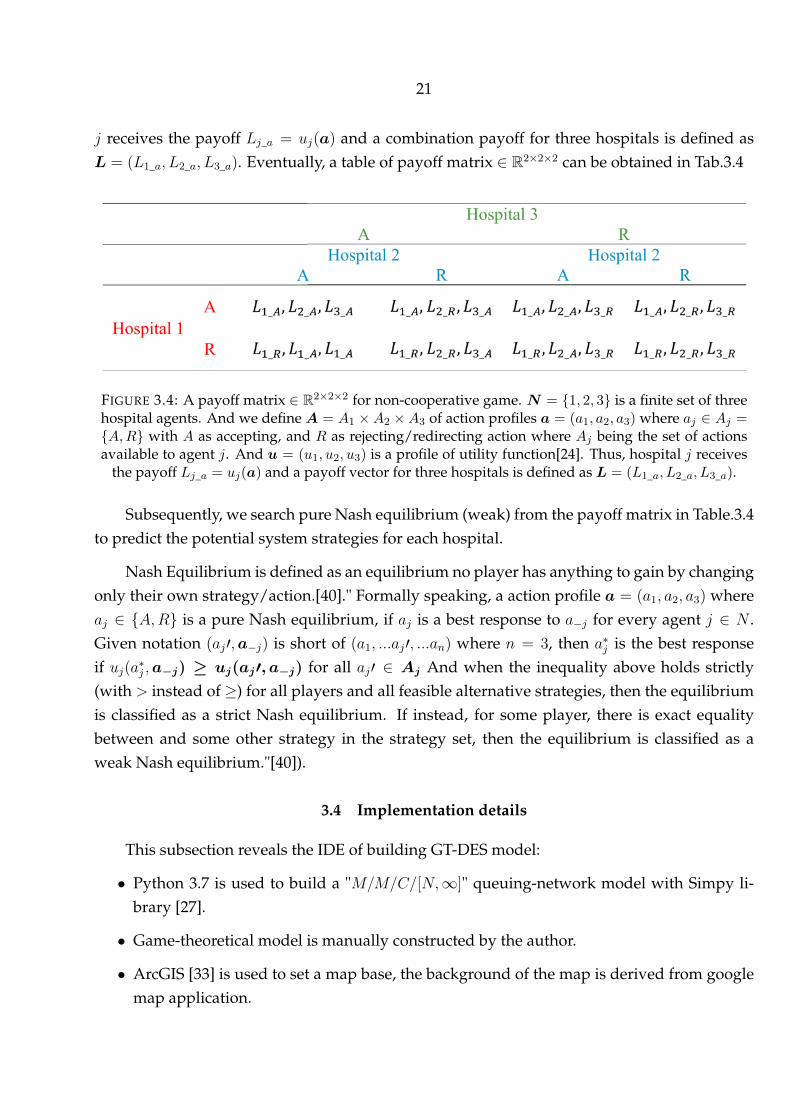
j receives the payoff Lj_a = uj(a) and a combination payoff for three hospitals is defined asL = (L1_a, L2_a, L3_a). Eventually, a table of payoff matrix ∈ R2×2×2 can be obtained in Tab.3.4

FIGURE 3.4: A payoff matrix ∈ R2×2×2 for non-cooperative game. N = 1, 2, 3 is a finite set of threehospital agents. And we define A = A1 × A2 × A3 of action profiles a = (a1, a2, a3) where aj ∈ Aj =A,R with A as accepting, and R as rejecting/redirecting action where Aj being the set of actionsavailable to agent j. And u = (u1, u2, u3) is a profile of utility function[24]. Thus, hospital j receives

the payoff Lj_a = uj(a) and a payoff vector for three hospitals is defined as L = (L1_a, L2_a, L3_a).

Subsequently, we search pure Nash equilibrium (weak) from the payoff matrix in Table.3.4to predict the potential system strategies for each hospital.

Nash Equilibrium is defined as an equilibrium no player has anything to gain by changingonly their own strategy/action.[40]." Formally speaking, a action profile a = (a1, a2, a3) whereaj ∈ A,R is a pure Nash equilibrium, if aj is a best response to a−j for every agent j ∈ N .Given notation (aj′,a−j) is short of (a1, ...aj′, ...an) where n = 3, then a∗j is the best responseif uj(a∗j ,a−j) ≥ uj(aj′, a−j) for all aj′ ∈ Aj And when the inequality above holds strictly(with > instead of ≥) for all players and all feasible alternative strategies, then the equilibriumis classified as a strict Nash equilibrium. If instead, for some player, there is exact equalitybetween and some other strategy in the strategy set, then the equilibrium is classified as aweak Nash equilibrium."[40]).

3.4 Implementation details

This subsection reveals the IDE of building GT-DES model:

• Python 3.7 is used to build a "M/M/C/[N,∞]" queuing-network model with Simpy li-brary [27].

• Game-theoretical model is manually constructed by the author.

• ArcGIS [33] is used to set a map base, the background of the map is derived from googlemap application.

22

• A library SALib [15] is used for sensitivity analysis.

3.5 Scenario design

This section depicts a specific scenario for GT-DES model’s simulation. We firstly set thebasic environment of the model. Secondly, we invoked two types of agents: patient and hos-pital. Each of them is associated with self properties and event-triggered operations [45]. Theidea of designing the computational model is based on Object-modelling technique (OMT)[37]. The biggest strength of using OMT is the computational model can be easily developedby object-oriented programming (OOP) such as Python.

Environment design

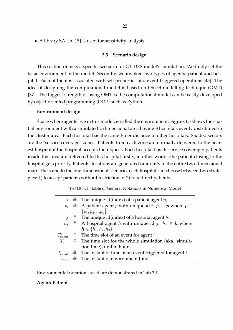
Space where agents live in this model, is called the environment. Figure.3.5 shows the spa-tial environment with a simulated 2-dimensional area having 3 hospitals evenly distributed inthe cluster area. Each hospital has the same Euler distance to other hospitals. Shaded sectorsare the "service coverage" zones. Patients from each zone are normally delivered to the near-est hospital if the hospital accepts the request. Each hospital has its service coverage: patientsinside this area are delivered to this hospital firstly, in other words, the patient closing to thehospital gets priority. Patients’ locations are generated randomly in the entire two-dimensionalmap. The same to the one-dimensional scenario, each hospital can choose between two strate-gies: 1) to accept patients without restriction or 2) to redirect patients.

TABLE 3.1: Table of General Notations in Numerical Model

i , The unique id(index) of a patient agent pipi , A patient agent p with unique id i. pi ∈ p where p ∈

p1, p2, ...pnj , The unique id(index) of a hospital agent hjhj , A hospital agent h with unique id j. hj ∈ h where

h ∈ h1, h2, h3T ievent , The time slot of an event for agent iTenv , The time slot for the whole simulation (aka. simula-

tion time), unit in hourtievent , The instant of time of an event triggered for agent itenv , The instant of environment time

Environmental notations used are demonstrated in Tab.3.1.

Agent: Patient

23

FIGURE 3.5: Simulated two-dimensional area with three hospitals and correspond-ing capacity of servers.Shaded sectors are the "service coverage" zones. Parametersused are Radius = 40km, origin = (40, 40), and locations of hospitals are Ph =

[[20.9014, 28.9734], [59.0985, 28.9734], [40, 62.0531]].

24

The patient is a core role throughout the model. The general term "patient" could be seen asa class with attributes as shown in Tab3.2. Each instance of a patient with a unique ID is namedas a process in SimPy (A python library to model discrete-event simulation as explained insection 3.4). Therefore, as the inner clock env.time starts counting, we first construct a generatorprocess to create patient process whenever "request event" is triggered. Next, each patientinstance (process) starts moving immediately.

TABLE 3.2: Table of Attribute Notations of Agent: Patient

pi , A patient agent p with unique id i. pi ∈ p where p ∈p1, p2, ...pn

T itravelling , The duration of time spent in travelling from the placepatient was fetched to target hospital hj where j ∈1, 2, 3

T iqueue , The duration of time spent by a patient i in queuing atwaiting room of hospital

T iserving , The duration of time spent by a patient i from beingserved till discharged

pi.status , The statues of patient going to target hospital,pi.status ∈ Direct, Redirect

pi.targetHos , The current target hospital of patient pi

Agent: Hospital

Hospitals are initialised at the beginning of simulation with associated properties shownin Tab.3.3

TABLE 3.3: Table of Attribute Notations of Agent: Hospital

hj , A hospital agent h with unique id j. hi ∈ h whereh ∈ h1, h2, h3

hj.strategy , The strategy hospital j is taking, in Accept, Redirecthj.res , A sub property of hospital indicating resource where

patient can request.hj.count , The number of users for resource(server) in hospital

hjhj.capacity , The number of maximum users in resource in hospital

hj , equal to the number of servers.hj.queue , The number of patients queuing for resource(server).

hj.maxQueue , The number of maximum length of queue in hospitalhj . If hj.strategy == Accept, hj.maxQueue = ∞, elsehj.maxQueue is predefined.

25

Algorithm: Searching for Nash Equilibrium

Result: Search weak Nash Equilibriumbegin

for a1 in a, a−1 dofor a2 in a, a−1 do

for a3 in a, a−1 do

if ua1,a2,a31 ≥ ua−11 ,a2,a3

1 and ua1,a2,a32 ≥ ua1,a

−12 ,a3

2 and ua1,a2,a33 ≥ ua1,a2,a

−13

2 thena1, a2, a3 is weak Nash Equilibrium

end

end

end

endAlgorithm 1: Search 3-d weak Nash Equilibrium

This part formally explain the computational process to obtain the Nash Equilibrium forGT-DES model. The general idea is: with running r realisations of GT-DES models by MonteCarlo simulations, we obtain a list of Nash Equilibrium, where the most frequent strategycombination is selected as Nash Equilibrium in given scenario.

Formally speaking, given generated fixed patients lists pi = [p1, p2, . . . , pfi) where eachpi associated with random request time and serving time under the restrain that the averagerequest and serving rate is λ,M . The length of pi is cut off by the end of simulation time. Next,the GT-DES model is considered as a function fi(λ,M, a,pi = [p1, p2, . . . , pfi) which returns aninstance of payoff L = (L1_a, L2_a, L3_a) described in section3.3, where a = [AAA, .., RRR] anda ∈ AAA, .., RRR. So that the payoff matrix could be obtained by

fi(λ,M,a,pi) =

fi(λ,M, a = [AAA],pi = [p1, p2, . . . , pfi)

fi(λ,M, a = [AAR],pi = [p1, p2, . . . , pfi)...

fi(λ,M, a = [RRA],pi = [p1, p2, . . . , pfi)

fi(λ,M, a = [RRR],pi = [p1, p2, . . . , pfi)

(3.10)

Thus, with r random realisations of simulation, N (f(λ,M,a,p])) returns a list of NashEquilibrium (length = r where N(f1(λ,M,a,p1)) returns a instance of Nash Equilibrium byAlg.1. So that we have:

26

N (f(λ,M,a,p])) =

N(f1(λ,M,a,p1))

N(f2(λ,M,a,p2))...

N(fi(λ,M,a,pi))...

N(fr−1(λ,M,a,pr−1))

N(fr(λ,M,a,pr))

(3.11)

Eventually we obtain the Nash Equilibrium anewhere ane = argmaxP (ane|N (f(λ,M,a,p])))

where P denotes the probability density function.

3.6 Sensitivity analysis by the Sobol method

Sensitivity analysis (SA) is a method conducted to quantitatively performances how muchthe effect of the output comes from each input to model[38]. Three reasons we apply SA toGT-DES model are:

1. To increase the understanding between the inputs and output of a model

2. Find potentially useless inputs.

3. Robustness check and validation for model

Sobol indices (or Sobol method) is utilised to SA for GT-DES model [39]. Sobol is anvariance-based sensitivity analysis technique with following advantages [38]:

1. Sobol indices is a global method, meaning either independent interacted influence ofinputs can be performed.

2. Passing Sobol method to Non-linear process in simulation is not a problem

To formally perform Sobol method, we want to obtain the first and total order indices.With i being the index of one of the inputs, Y being the target outcome of the model, the first-order indices (S1) is :

Si =Di

var(Y )(3.12)

whereDi(Y ) = V ar[E(Y |Xi)] (3.13)

Interaction indices is:sij =

Dij

V ar(Y )(3.14)

27

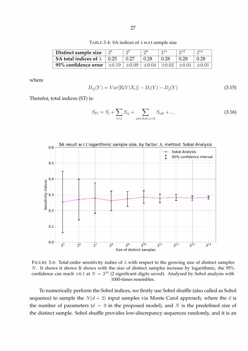
TABLE 3.4: SA indices of λ w.r.t sample size

Distinct sample size 25 27 29 211 213 214

SA total indices of λ 0.25 0.27 0.28 0.28 0.28 0.2895% confidence error ±0.19 ±0.09 ±0.04 ±0.02 ±0.01 ±0.01

whereDij(Y ) = V ar[E(Y |Xi)]−Di(Y )−Dj(Y ) (3.15)

Therefor, total indices (ST) is:

ST i = Si +∑i<j

Sij +∑

j 6=i,k 6=i,j<k

Sijk + ... (3.16)

FIGURE 3.6: Total-order sensitivity indies of λ with respect to the growing size of distinct samplesN . It shows it shows It shows with the size of distinct samples increase by logarithmic, the 95%confidence can reach ±0.1 at N = 214 (2 significant digits saved). Analysed by Sobol analysis with

1000-times resembles.

To numerically perform the Sobol indices, we firstly use Sobol shuffle (also called as Sobolsequence) to sample the N(d + 2) input samples via Monte Carol approach; where the d isthe number of parameters (d = 9 in the proposed model), and N is the predefined size ofthe distinct sample. Sobol shuffle provides low-discrepancy sequences randomly, and it is an

28

efficient sampling method. As N grows, the computational cost increase linearly by O(n). Todetermine the size of the distinct sample, N , as shown in Figure.3.6, with the size of distinctsamples increase by logarithmic, the 95% confidence error can reach ±0.1 at N = 214 as shownin tab.3.4 with two significant digits saved. Thus, the Sobol indices with N = 214 will beperformed.

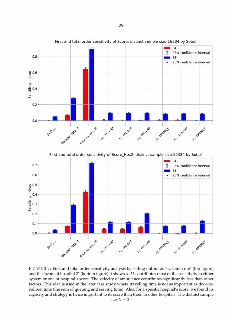
Next, we performed the Sobol method by setting output as "Score" and the "Score of thehospital 2" as shown in the Figure.3.7. The "Score" of hospital j is defined as

Scorej =njservedT jtotal

(3.17)

Where njserved is the number of patients being served in hospital j within the simulation time,it shows λ,M contributes most of the sensitivity to either system or one of hospital’s score.The velocity of ambulance contributes significantly less than other factors. This idea is used inthe later case study where travelling time is not as important as door-to-balloon time (the sumof queuing and serving time). Also, for a specific hospital’s score, we found its capacity andstrategy is twice important to its score than them in other hospitals.

29

FIGURE 3.7: First and total order sensitivity analysis by setting output as "system score" (top figure)and the "score of hospital 2" (bottom figure).It shows λ,M contributes most of the sensitivity to eithersystem or one of hospital’s score. The velocity of ambulance contributes significantly less than otherfactors. This idea is used in the later case study where travelling time is not as important as door-to-balloon time (the sum of queuing and serving time). Also, for a specific hospital’s score, we found itscapacity and strategy is twice important to its score than them in other hospitals. The distinct sample

size N = 214

30

4 EXPERIMENTAL STUDY AND RESULTS

This section presents the results of a one-dimensional mathematical model, two-dimensionalstochastic GT-DES model. Secondly, an application of GT-DES model for simulating the ambu-lance dispatching of ACS patients in Saint Petersburg is discussed, with real-world data beingused.

4.1 Simulating with artificial settings

4.1.1 Warm-up simulation

FIGURE 4.1: Global time spent at two hospitals of a one-dimensional queuing-network model. "A"in the legend stands for accepting strategy, "R" denotes redirecting strategy. The less global time, thebetter to the system. It shows AA strategy is the most beneficial strategy (with dominantly less globaltime) in most cases, except the circled interaction in the left figure; where AA switches to RA and RR,and it starts to reduce the global time when patients flow grows to a certain level, given the server

N =N1, N2 = [2, 1] is not equal. Parameter used are Tc=6, patient flow is defined as λµ1+µ2

The warm-up simulation contains a simple simulation of 1d and 2d queuing-networkmodel.

Firstly, we run a batch of computationally-cheap simulations to check the truth of the 1Dmodel quickly. Some insightful results have caught our eyes: Figure.4.1 presents the globaltime spent by all patients for two hospitals( the less global time, the better to the system). Itshows AA strategy is the most beneficial strategy (with dominantly less global time) in most

31

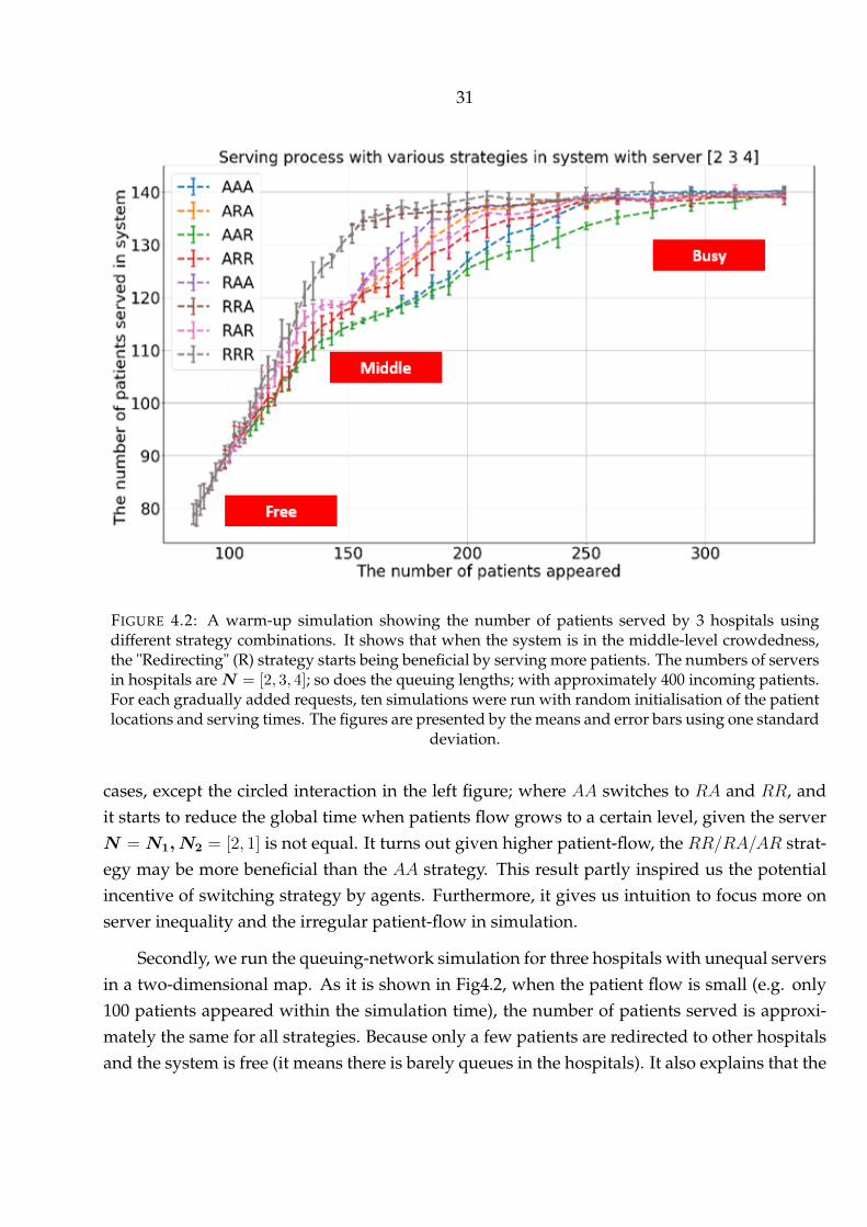
FIGURE 4.2: A warm-up simulation showing the number of patients served by 3 hospitals usingdifferent strategy combinations. It shows that when the system is in the middle-level crowdedness,the "Redirecting" (R) strategy starts being beneficial by serving more patients. The numbers of serversin hospitals areN = [2, 3, 4]; so does the queuing lengths; with approximately 400 incoming patients.For each gradually added requests, ten simulations were run with random initialisation of the patientlocations and serving times. The figures are presented by the means and error bars using one standard

deviation.

cases, except the circled interaction in the left figure; where AA switches to RA and RR, andit starts to reduce the global time when patients flow grows to a certain level, given the serverN = N1, N2 = [2, 1] is not equal. It turns out given higher patient-flow, the RR/RA/AR strat-egy may be more beneficial than the AA strategy. This result partly inspired us the potentialincentive of switching strategy by agents. Furthermore, it gives us intuition to focus more onserver inequality and the irregular patient-flow in simulation.

Secondly, we run the queuing-network simulation for three hospitals with unequal serversin a two-dimensional map. As it is shown in Fig4.2, when the patient flow is small (e.g. only100 patients appeared within the simulation time), the number of patients served is approxi-mately the same for all strategies. Because only a few patients are redirected to other hospitalsand the system is free (it means there is barely queues in the hospitals). It also explains that the

32

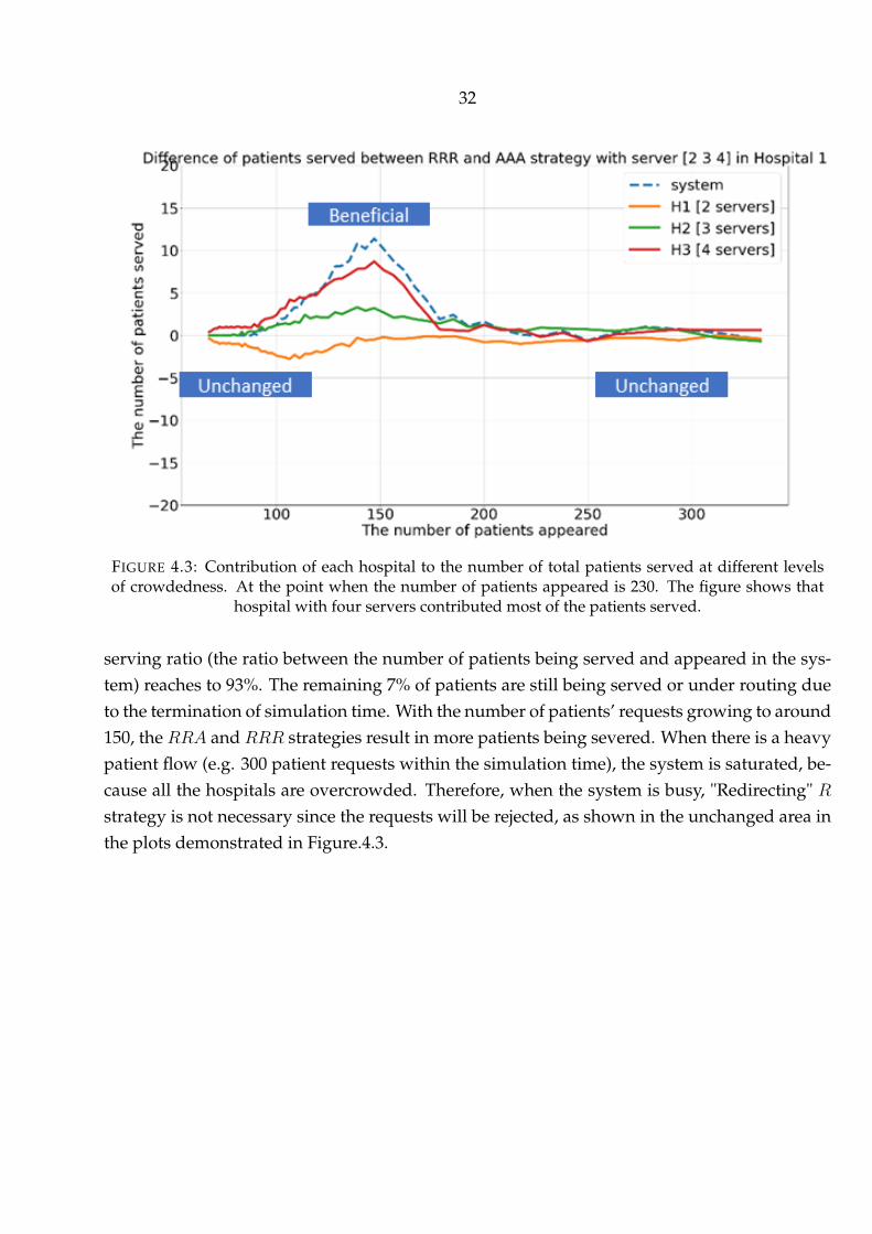
FIGURE 4.3: Contribution of each hospital to the number of total patients served at different levelsof crowdedness. At the point when the number of patients appeared is 230. The figure shows that

hospital with four servers contributed most of the patients served.

serving ratio (the ratio between the number of patients being served and appeared in the sys-tem) reaches to 93%. The remaining 7% of patients are still being served or under routing dueto the termination of simulation time. With the number of patients’ requests growing to around150, the RRA and RRR strategies result in more patients being severed. When there is a heavypatient flow (e.g. 300 patient requests within the simulation time), the system is saturated, be-cause all the hospitals are overcrowded. Therefore, when the system is busy, "Redirecting" Rstrategy is not necessary since the requests will be rejected, as shown in the unchanged area inthe plots demonstrated in Figure.4.3.

33

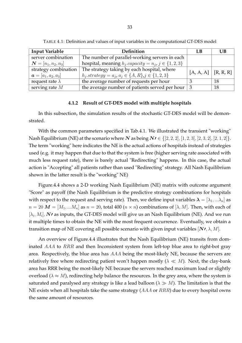
TABLE 4.1: Definition and values of input variables in the computational GT-DES model

Input Variable Definition LB UBserver combinationN = [n1, n2, n3]

The number of parallel-working servers in eachhospital, meaning hj.capacity = nj , j ∈ 1, 2, 3

strategy combinationa = [a1, a2, a3]

The strategy taking by each hospital, wherehj.strategy = aj , aj ∈ A,R,j ∈ 1, 2, 3

[A, A, A] [R, R, R]

request rate λ the average number of requests per hour 3 18serving rate M the average number of patients served per hour 3 18

4.1.2 Result of GT-DES model with multiple hospitals

In this subsection, the simulation results of the stochastic GT-DES model will be demon-strated.

With the common parameters specified in Tab.4.1. We illustrated the transient "working"Nash Equilibrium (NE) at the scenario whereN as beingN ′ ∈ [2, 2, 2], [1, 2, 3], [2, 3, 2], [2, 1, 2].The term "working" here indicates the NE is the actual actions of hospitals instead of strategiesused (e.g. it may happen that due to that the system is free (higher serving rate associated withmuch less request rate), there is barely actual "Redirecting" happens. In this case, the actualaction is "Accepting" all patients rather than used "Redirecting" strategy. All Nash Equilibriumshown in the latter result is the "working" NE)

Figure.4.4 shows a 2-D working Nash Equilibrium (NE) matrix with outcome argument"Score" as payoff (the Nash Equilibrium is the predictive strategy combinations for hospitalswith respect to the request and serving rate). Then, we define input variables λ = [λ1, ...λn] asn = 20M = [M1, ...Mn] as n = 20, total 400 (n × n) combinations of [λ,M ]. Then, with each of[λi,Mi],N ′ as inputs, the GT-DES model will give us an Nash Equilibrium (NE). And we runit multiple times to obtain the NE with the most frequent occurrence. Eventually, we obtain atransition map of NE covering all possible scenario with given input variables [N ′, λ,M ].

An overview of Figure.4.4 illustrates that the Nash Equilibrium (NE) transits from dom-inated AAA to RRR and then Inconsistent system from left-top blue area to right-bot grayarea. Respectively, the blue area has AAA being the most-likely NE, because the servers arerelatively free where redirecting patient won’t happen mostly (λ M ). Next, the clay-bankarea has RRR being the most-likely NE because the servers reached maximum load or slightlyoverload (λ ≈M ), redirecting help balance the resources. In the grey area, where the system issaturated and paralysed any strategy is like a lead balloon (λ M ). The limitation is that theNE exists when all hospitals take the same strategy (AAA or RRR) due to every hospital ownsthe same amount of resources.

34

FIGURE 4.4: A 2-D working Nash Equilibrium (NE) matrix with outcome argument "Score" as thepayoff. given λ = [3, 18],M = [3, 18] in the scenario of N = [2, 2, 2] (left) and N = [2, 1, 2] (right).It shows with growing request rate (λ) and declining serving rate (M ), the pure Nash Equilibriumtransits from AAA to RRR until the system is inconsistent. The term "inconsistent" (abbr. "InconSys", shown as grey square in the plot) states there is no NE due to the system being overcrowded(meaning queuing time goes to infinite in EACH hospital for incoming patients). Each block showsthe most frequent Nash Equilibrium among all 106 realisations The area of a coloured inner squaredivided by 1 is the probability of occurrences (i.e. the probability of AAA strategy being NE at theleft-top corner is 100%). And each NE is searched from payoff matrix 3.4 by algorithm 1, Simulationparameters used are: 106 simulations for each block (20 × 20 = 400 rectangles in total), simulationtime ranges from 30 to 135hours, the appeared number of patients ranges from 400 to 2500, vamb =

50km/hour, hi.maxQueue = [2, 2, 2]

35

FIGURE 4.5: An arbitrary example of the dispersive distribution for the occurrence of Nash Equilib-rium in a simulation. In this case, the RRR strategy is selected as Nash Equilibrium due to RRR

appeared 17.92% in 106 simulations.

To elaborate the story at strategy transition, a zoomed-in distribution at red-circled rectan-gle in Figure.4.4 is demonstrated in Figure.4.5. Stochastically, the NE distribution is dispersivewhere RRR is slightly more chance of being NE (17.92%) than AAA (16.04%)

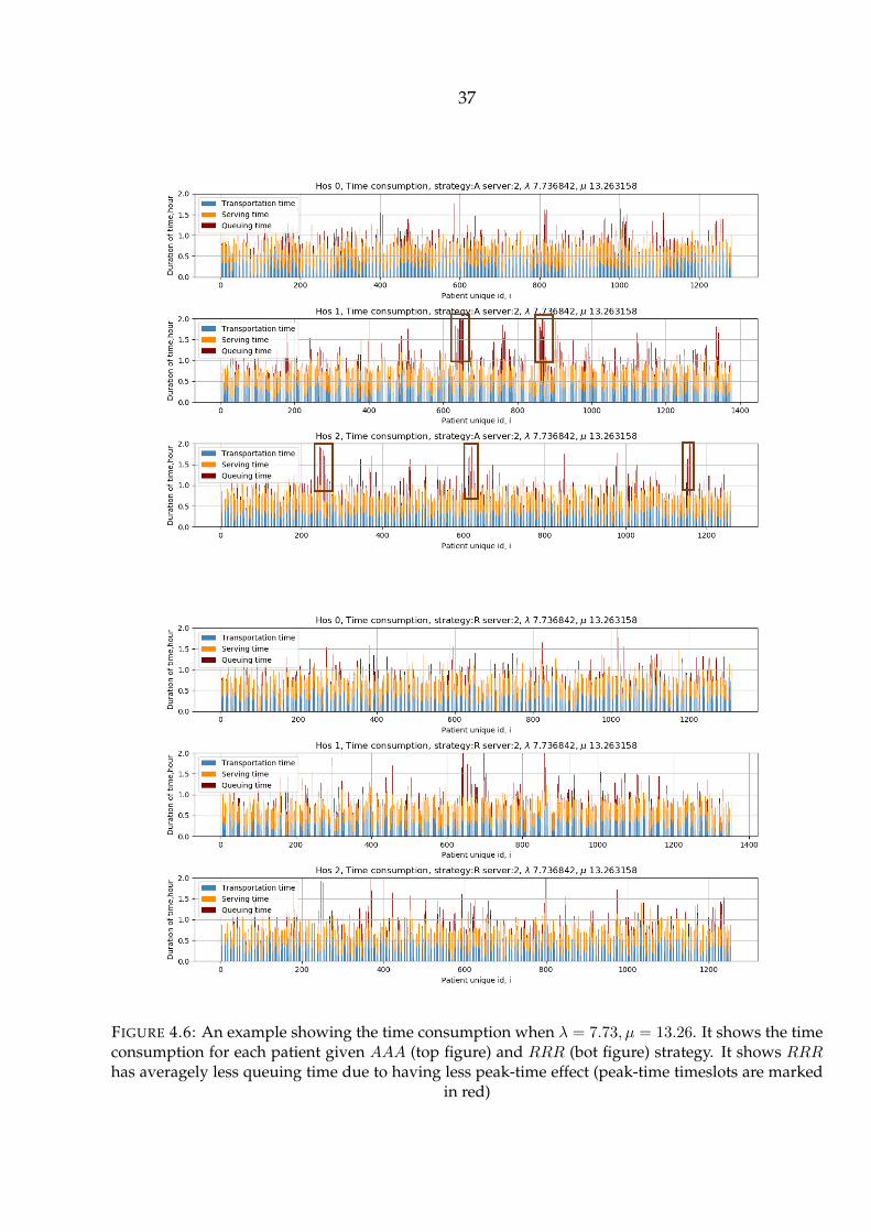
Next, we plotted the time consumption of each patient in each hospital, shown in Fig-ure.4.6. At peak-time period, there is overcrowding in the system which contributes higherqueuing time as shown in the top plot having rectangles area.

The bottom figure in Figure.4.4 reveals the NE transition in the scenario of N = [2, 1, 2]. Itshows the equilibrium transits from AAA ⇒ ARA ⇒ RRR ⇒ RAR ⇒ Inconsistent. It turnsout, when one hospital having less server while others have more same number of servers,the hospital with less server starts switching R strategy with growing request rate (Dark greenarea). However, when system is slightly overload, it firstly switched to A strategy then others.

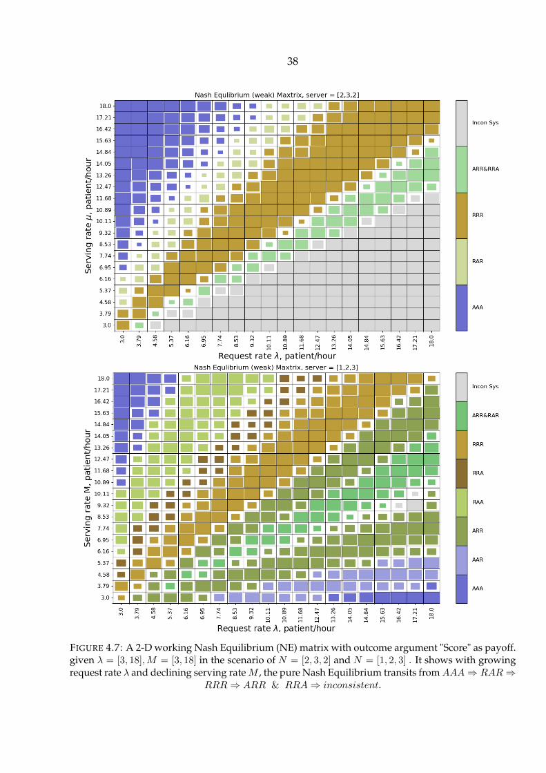
Figure.4.7 reveals the NE transition in the scenario of N = [2, 3, 2]. Likewise, hospital withfewer server are more vulnerable to environment and strategy switched firstly from Acceptingto Redirecting via AAA ⇒ RAR ⇒ RRR ⇒ ARR & RRA ⇒ inconsistent. As well as thebottom figure in Figure.4.7.

To summarise, we see that 1. The system strategy transits from more Accepting to moreRedirecting as the system gets busy. 2. The hospital with fewer servers tends to switch strategy

36

earlier than the one with more servers. These two findings can be verified in the later casestudy of ACS patients in Saint Petersburg.

37

FIGURE 4.6: An example showing the time consumption when λ = 7.73, µ = 13.26. It shows the timeconsumption for each patient given AAA (top figure) and RRR (bot figure) strategy. It shows RRRhas averagely less queuing time due to having less peak-time effect (peak-time timeslots are marked

in red)

38

FIGURE 4.7: A 2-D working Nash Equilibrium (NE) matrix with outcome argument "Score" as payoff.given λ = [3, 18],M = [3, 18] in the scenario of N = [2, 3, 2] and N = [1, 2, 3] . It shows with growingrequest rate λ and declining serving rateM , the pure Nash Equilibrium transits fromAAA⇒ RAR⇒

RRR⇒ ARR & RRA⇒ inconsistent.

39

4.2 Simulating ambulance dispatching of ACS patients in Saint Petersburg

This subsection demonstrates the case study of GT-DES model on ACS patients in SaintPetersburg with real-world data set involved. We firstly simulate the isolated area (with only0_hos and 1_hos). Secondly, we simulate every available pair of hospitals and predict theirstrategies by finding the Nash Equilibrium. The hospital pairs are selected by consideringthe proportion of shared patients by each of hospital in the pair. Thirdly, we calculate theweighted strategy for each hospital and predict the global strategy (the strategy combinationfor all hospitals in the city).

In order to understand the treatment of Acute coronary syndrome (ACS) patients by thehealth-care system in Saint Petersburg, a simulation supported with real-world datasets will beintroduced. Firstly, the background and the datasets will be discussed. Secondly, methods ofsimulating request process, travel process, the serving process of ACS patients with involvingthe real-world dataset will be explained. Thirdly, we applied the GT-DES model to simulatethe ambulance dispatching for an isolated area with two hospitals as a start point. Then weextend the simulation for every interacting hospital’s pair in the city. An interacting hospitalpair such as ihos and jhos means there exist an area where patients are going to either ihos andjhos. (usually, ihos and jhos are neighbouring). As a result, the average door-to-balloon timein each hospital is measured. And the average mortality in a year is estimated by the door-to-balloon time. Subsequently, we compared the simulated mortality with observed mortalityfrom data as validation. In future, a deep understanding of the ACS case can result in furtherresearch in policy-making for the lower mortality of ACS patients in Saint Petersburg.

4.2.1 Background

Acute coronary syndrome (ACS) is a syndrome where the patient’s heart may not be func-tioning properly due to decreased blood flow in the coronary arteries [2]. We choose ACSpatients for simulation because they have two main properties: professional aids in hospital isneeded, ACS occurs in an unexpected situation. Also, the angiography is set up as a server inthe model because 1. an angiography is a must-have surgery resource as an imaging techniquefor ACS patient two due to the high price, most hospitals do not own a sufficient amount ofangiography and supporting resource. Meanwhile, other types of urgent patients may also oc-cupy the server due to angiography is a universal framework for heart diseases, such as Acutemyocardial infarction (AMI), stent and stroking. Thus, sometimes ACS patients have to bewaiting during rush hour, extra time spent can lead to higher mortality in the hospital whichis not expected in the health-care system.

40

4.2.2 Data description

Almazov National Medical Research Centre provides the data in Saint Petersburg. We areauthorised to use them for internal research only.

Datasets contain :

1. 5124 records of ACS patients went to Thirteen hospitals by ambulance from 1th Jan to 15thNov in 2015 in Saint Petersburg. This dataset can be used to build the request process ofACS patients for simulation.

2. Thirteen hospitals linked to the records of patients and the number of angiographies eachhospital has. This dataset is used to set up the simulation environment to support pa-tients’ travel process and serving process.

3. 1,310,263 travelling time records of vehicles spread in Saint Petersburg from 143 locationsto 18 other locations (including 13 hospitals) at each hour. This dataset is used to simulatethe travel process.

4. Serving time for 1866 records of stent patients.This dataset is used to simulate the servingprocess of ACS patients.

5. Annual averaged mortality in 2015 of 10 hospitals in Saint Petersburg. This dataset isused for model validation (as an comparison to the simulated mortality)

41

4.2.3 Scenarios

In this section, methods of simulating request process, travel process, the serving processof ACS patients will be explained.

Simulation environment

Figure.4.8 shows the locations of the 11 hospitals and the number of incoming patients(5124 records in total) in Saint Petersburg. It should be addressed there is more ACS patients inrealistic than we recorded in Saint Petersburg in 2015 because the city ambulance recorded byEMS arranges only roughly 20% of patients, and the rest of patients are delivered by hospital’sprivate ambulance, reported by the doctors in Saint Petersburg. Also in our dataset, we initiallyhave information of 13 hospitals rather than 11. The remaining two hospitals are not adoptedin the model because they have small patient inflow and not operating 24/7 during the periodof observation.

Figure.4.9 shows the modelled hospitals in a rectangular area. We select this area for thereasons: 1. Modelling the whole city with unbalanced density is beyond complicated. 2. ACSpatients in the rectangular area (0_hos and 1_hos) are segregated from other areas (e.g. a riverkeeps back the area from the main island). 3. patients in Pushkin and Kolpino area are lessinfluential by delivering time so that they are excluded

4.2.4 Simulation Results

This section explains an application of GT-DES model applied to a real-world scenario.

Modelling ACS patients in Saint Petersburg

This section depicts the methods of data analysis exploration, fitting the data and artificialdata generation.

Request process

Arrival process models sending the patient’s request to hospitals. Figure.4.10 plots theinterval time of patients’ requests derived from data. It shows the time interval of patientsrequests can be fitted by an exponential distribution with λ = 0.6911, meaning the averageinterval between ACS patient’s request to the medical centre (EMS) is 1

λ≈ 1.4470 hours in

Saint Petersburg from January to November in 2015.

However, in real life, the health-care system will not be as simple as we modelled. Atypical finding is that the request rate λ varies hourly, as shown in Figure.4.11. The figure

42

FIGURE 4.8: Eleven hospitals having angiography in Saint Petersburg (using index instead of realhospital names). Hospitals work 24/7 and 5124 patients going to each of them. Background map isderived from Google Map application. The scale of map is 1km : 1, and 1 yard of latitude equals

111.111km on real world.

shows the rush hour of receiving the request is roughly at around noon. And at 6 am, therewill be fewer requests.

Thus, in the numerical implementation, we firstly extract the hourly average request ratesλd = λh where h ∈ 0, 1, 2..., 23 from records in selected area. Next, the request rate λ at

43

FIGURE 4.9: Patient selected for local simulation in an isolated rectangular area

FIGURE 4.10: Plotted histogram for Tinterval of patients’ requests from our data (5124 records of ACSpatients made calls to EMS). Figure shows the time interval of patients appearances can be fitted byexponential distribution with λ = 0.6911, meaning the average of interval between ACS patient’s

request is 1λ ≈ 1.4470 hours both 4 digits saved.

44

FIGURE 4.11: The average number of requests per hour in a day to Almazov medical centre from01/01/2015 to 15/11/2015. It shows the request rate changes hourly in a day: the rush hour of receiv-

ing request is roughly at around noon. And at 6 am, there will be fewer requests on average.

current time t.env is computed by λ = λh where h = tenv. And to avoid the geographical bias,the simulated patients locations are extracted from recorded data.

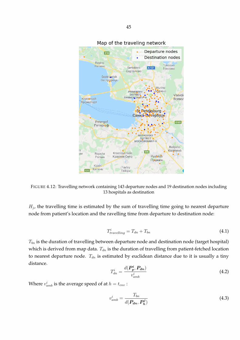
Travel process This section explains the estimation of travelling time of each patient totarget hospital. Instead of estimating travelling time by Euclidean distance in the stochasticmodel, travelling time is estimated from map data here. Travelling time data can be seen asa directed travelling network. 1,310,263 travelling time records are the directed edges linking143 departure nodes to 19 destination nodes (including 13 hospitals), as shown in Figure.4.12.

Figure.4.13 shows the average travelling time hourly for all the available connections. Twopossible explanations for the source of error are:

• peak hours exists. E.g. transportation is busy in main roads.As shown in Figure.4.13, We found the time period at 9 am or between 6 pm, and 7 pmare the peak hours in Saint Petersburg where travelling time grows. It turns out whileestimating travelling time, the rush hour of daily routing shall be carefully considered.

• Even at the same hour, the average velocity changes because of geographical and socialeffects [19].

In this case, the travelling time for the patient is estimated by the collected map data anda supplemented straight-line method. Formally speaking, with patient pi travelling to hospital

45

FIGURE 4.12: Travelling network containing 143 departure nodes and 19 destination nodes including13 hospitals as destination

Hj , the travelling time is estimated by the sum of travelling time going to nearest departurenode from patient’s location and the ravelling time from departure to destination node:

T itravelling = Tdn + Tbn (4.1)

Tbn is the duration of travelling between departure node and destination node (target hospital)which is derived from map data. Tdn is the duration of travelling from patient-fetched locationto nearest departure node. Tdn is estimated by euclidean distance due to it is usually a tinydistance.

T idn =d(P i

p,Pdn)

viamb(4.2)

Where viamb is the average speed of at h = tenv :

viamb =Tbn

d(Pdn,Pjh)

(4.3)

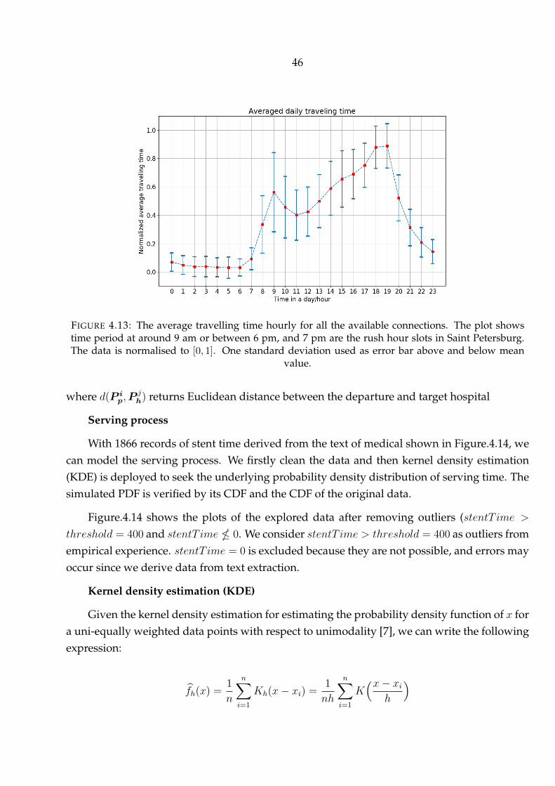
46

FIGURE 4.13: The average travelling time hourly for all the available connections. The plot showstime period at around 9 am or between 6 pm, and 7 pm are the rush hour slots in Saint Petersburg.The data is normalised to [0, 1]. One standard deviation used as error bar above and below mean

value.

where d(P ip,P

jh) returns Euclidean distance between the departure and target hospital

Serving process

With 1866 records of stent time derived from the text of medical shown in Figure.4.14, wecan model the serving process. We firstly clean the data and then kernel density estimation(KDE) is deployed to seek the underlying probability density distribution of serving time. Thesimulated PDF is verified by its CDF and the CDF of the original data.

Figure.4.14 shows the plots of the explored data after removing outliers (stentT ime >

threshold = 400 and stentT ime 0. We consider stentT ime > threshold = 400 as outliers fromempirical experience. stentT ime = 0 is excluded because they are not possible, and errors mayoccur since we derive data from text extraction.

Kernel density estimation (KDE)

Given the kernel density estimation for estimating the probability density function of x fora uni-equally weighted data points with respect to unimodality [7], we can write the followingexpression:

fh(x) =1

n

n∑i=1

Kh(x− xi) =1

nh

n∑i=1

K(x− xi

h

)

47

FIGURE 4.14: Demonstration of stent time after removing outliers (stentT ime > threshold = 400 andstentT ime 0.

whereK is a selected kernel function (Gaussian function in this case because as the numberof data grows, the selection of kernel function does less impact to estimated density) under theassumptions of 1. non-negative K(x) ≥ 0 for every x 2. symmetric: K(x)= K(-x).

As h is the bandwidth, to scale the shape of kernel function. h is selected by Silverman orScott rules. Where in practice, the Silverman rule to obtain the bandwidth as hsm = 4σ5

3n

1/5. And

the Scotts rule hscoot = n−1/(d+4), Where n is the number of data points and d is the number ofdimensions (n = 1866, d = 1 for the dataset of stent time).

As a result shown in Figure.4.15, experimental fit of stent time shows the KDE method hasmostly closer fit and the algorithm for band width selection has less impact in the particularcase. Kolmogorov-Smirnov test (KS test) is used to verify the goodness of KDE fit. KStestdefinition: for a observed random variable x where G(x) is the cumulative results and F (x) isa given CDF. KStest hypothesised the two distributions are identical as G(x) = F (x).

To obtain the CDF of the KDE function, we have Kernel density estimation for probabilitydensity function of x for a unequally weighted data points with respect to unimodality :

fh(x) =1

n

n∑i=1

Kh(x− xi) =1

nh

n∑i=1

K(x− xi

h

)

Then the CDF of KDE function is

Fh(x) =1

nh

n∑i=1

FK

(x− xih

)

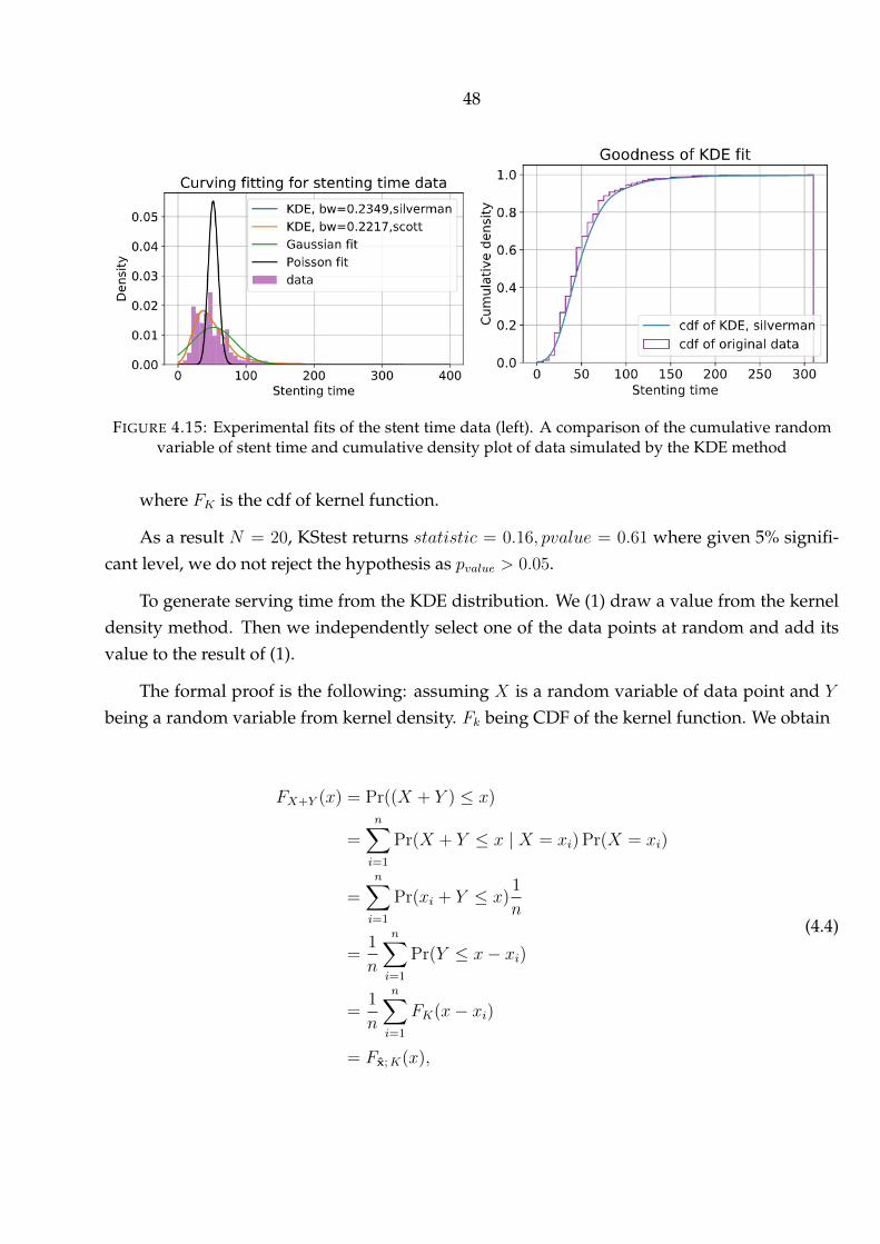
48

FIGURE 4.15: Experimental fits of the stent time data (left). A comparison of the cumulative randomvariable of stent time and cumulative density plot of data simulated by the KDE method

where FK is the cdf of kernel function.

As a result N = 20, KStest returns statistic = 0.16, pvalue = 0.61 where given 5% signifi-cant level, we do not reject the hypothesis as pvalue > 0.05.

To generate serving time from the KDE distribution. We (1) draw a value from the kerneldensity method. Then we independently select one of the data points at random and add itsvalue to the result of (1).

The formal proof is the following: assuming X is a random variable of data point and Y

being a random variable from kernel density. Fk being CDF of the kernel function. We obtain

FX+Y (x) = Pr((X + Y ) ≤ x)

=n∑i=1

Pr(X + Y ≤ x | X = xi) Pr(X = xi)

=n∑i=1

Pr(xi + Y ≤ x)1

n

=1

n

n∑i=1

Pr(Y ≤ x− xi)

=1

n

n∑i=1

FK(x− xi)

= Fx;K(x),

(4.4)

49

The game process is the same to the one in stochastic GT-DES model as explained in sec-tion.3.3.

Local simulation with isolated hospitals

This section depicts the simulation of two selected hospitals and corresponding patients inan isolated area. By looking at data, We see 0_hos accepts 57.63% of local patients and 43.7% ofpatients went to 1_hos with more facilities, but the workload is not ideally balanced. As 0_hoshas facility0 = 2 and 1_hos has facility1 = 1, the workload is not well balanced. Ideally, theratio between the patients in 0_hos and 1_hos shall approach 2 : 1

Firstly, we deployed the GT-DES model for 0_hos and 1_hos, and we obtained the pre-dicted Nash Equilibrium.

Figure.4.16 shows the probability of Nash Equilibrium for 0_hos and 1_hos (left) and re-verse (right) with respect to patient inflow. It shows the predicted strategy transit from AA toAR/RA and RR. It is reasonable according to our finding in the results of stochastic simula-tion, that is, hospitals with fewer servers tends to switch strategy firstly. Moreover, at a lowpatient inflow, "Accepting" strategy is preferred. Compared to the left and right figures, thesimulation is cross-verified because the Nash Equilibrium is symmetric except for the smallstochastic difference. Compared to the top and bot figures where the traffic jam is consideredand not, we found the traffic jam retreat the transition of Nash Equilibrium for lower patientinflow.

In addition, Figure.4.17 shows the Nash Equilibrium transition for selected 10_hos and3_hos and corresponding patients going to them. AA strategy dominated for any patient in-flow. That is reasonable because there are less patient in the north rather than patients in thesouth, meaning there is less competition for hospitals in the north of Saint Petersburg.

To summarise, the local simulations involving real-world data match our expectation of 1.The hospital with fewer servers switches strategy first. 2. Hospitals in the north tend to useAA strategy as there are fewer patients in the north in general.

Global simulation with all hospitals in Saint Petersburg

Next, we aim to simulate with each available hospital pair (5 is excluded due to 5_hos faraway from the urban area, and we tested the strategy of 5_hos is Accepting as expected).

Firstly, in order to find all the interactive hospital pairs, we filtered derive the proportion ofshared patient between each pair as the threshold. The proportion of shared patient is defined

50

FIGURE 4.16: The probability of Nash Equilibrium for 0_hos and 1_hos (left) and reverse (right) withrespect to patient inflow. The range of patient inflow is partitioned between max and min arrival rateof isolated patients in a day. 30 realisations for each patient inflow and 7200 hours simulation time foreach realisation. Also, 0_hos has facility0 = 2 and 1_hos has facility1 = 1 and the serving rate is 1.15patient per hour per server. Traffic jam is considered only for the top two figures. The hospital with

fewer servers 1_hos switches strategy first.

asPshread =

psharedPatptotal

where psharedPat is defined as the number of patients in the grided cell on map and ptotal are thenumber of patients targeting selected pair hospitals.

Figure.4.18 shows the proportion of shared patient for each available hospital pair Thepercentage of the shared patient for a duplicated hospital pair (e.g. 0hos and 0hos is 100%). Theplot shows that the proportion of shared patient is symmetric to the diagonal line as expected.

The following hospitals are filtered with the threshold = 0.05 of shared patients, meaningwith 5% or more shared patients, we assume the hospitals in a pair is interacting to the other.

[1_hos, 0_hos], [2_hos, 1_hos], [2_hos, 0_hos], [4_hos, 3_hos], [7_hos, 6_hos],

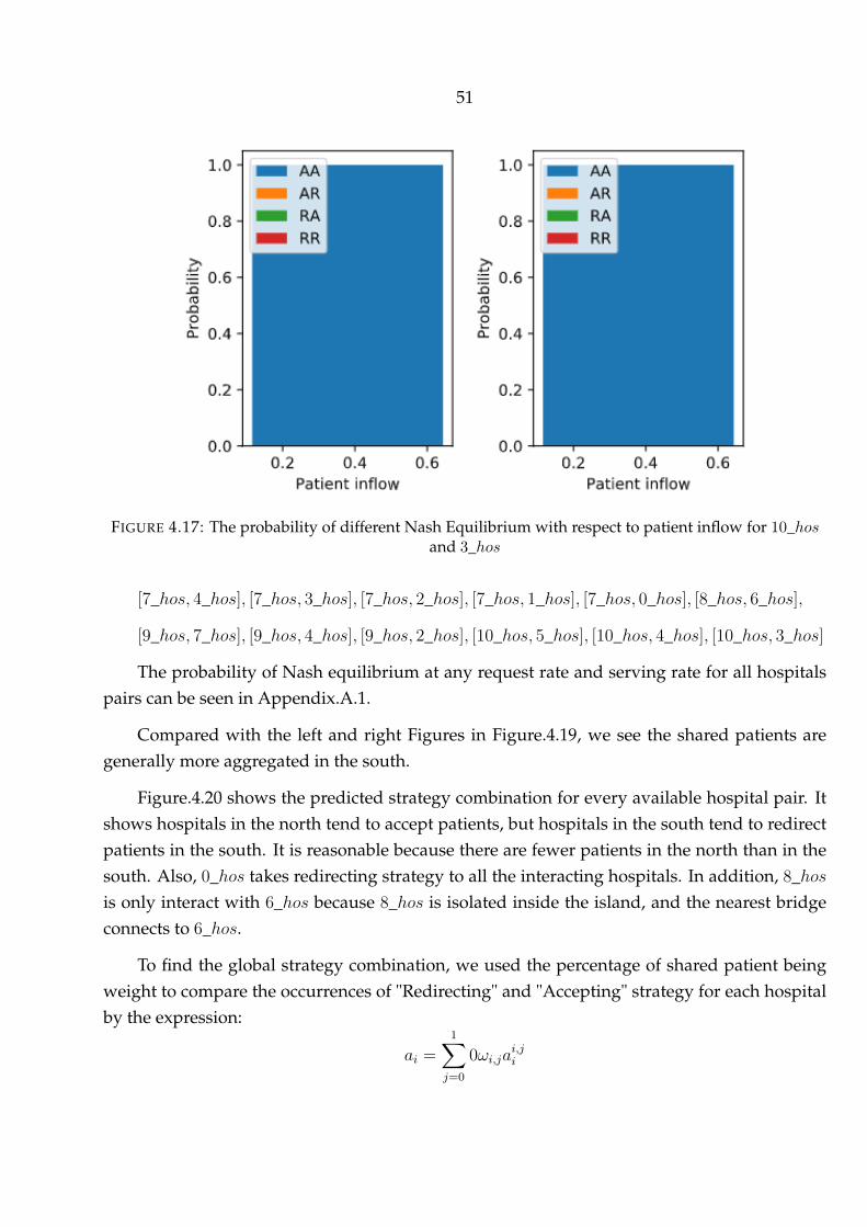
51

FIGURE 4.17: The probability of different Nash Equilibrium with respect to patient inflow for 10_hosand 3_hos

[7_hos, 4_hos], [7_hos, 3_hos], [7_hos, 2_hos], [7_hos, 1_hos], [7_hos, 0_hos], [8_hos, 6_hos],

[9_hos, 7_hos], [9_hos, 4_hos], [9_hos, 2_hos], [10_hos, 5_hos], [10_hos, 4_hos], [10_hos, 3_hos]

The probability of Nash equilibrium at any request rate and serving rate for all hospitalspairs can be seen in Appendix.A.1.

Compared with the left and right Figures in Figure.4.19, we see the shared patients aregenerally more aggregated in the south.

Figure.4.20 shows the predicted strategy combination for every available hospital pair. Itshows hospitals in the north tend to accept patients, but hospitals in the south tend to redirectpatients in the south. It is reasonable because there are fewer patients in the north than in thesouth. Also, 0_hos takes redirecting strategy to all the interacting hospitals. In addition, 8_hosis only interact with 6_hos because 8_hos is isolated inside the island, and the nearest bridgeconnects to 6_hos.

To find the global strategy combination, we used the percentage of shared patient beingweight to compare the occurrences of "Redirecting" and "Accepting" strategy for each hospitalby the expression:

ai =1∑j=0

0ωi,jai,ji

52

FIGURE 4.18: The heat map shows the proportion of the shared patients for every hospital pair.

where ai is the weighted action; ωi,j is the percentage of shared patient between i_hos andj_hos; ai,ji is the action of i_hos while interacting with j_hos independently. For any hospitali_hos where i = 0, 1, 2, 3, 4, 6, 7, 8, 9, 10, if the more weighted action is denoted as the primarystrategy of the hospital.

4.3 Interpretation, discussion and validation

In this section, we first validate the model by showing the comparative analysis of sim-ulated and observed mortality. Then we summarise our findings, ideas while applying theGT-DES model to simulating ACS patients in Saint Petersburg.

In practice, a key metric in the treatment of heart attacks is the door-to-balloon time. Itmeasures the interval starts with the patient’s arrival in the emergency department and endswhen a catheter guidewire crosses the culprit lesion in the Cardiac Catheterization lab [42].In the proposed GT-DES model, the door-to-balloon time of patient i measures the sum ofaveraged queuing and serving time as the following expression shows: Ti,DtB = Ti,queuing +

Ti,serving for hospital i_hos indexed by i for i = 0, 1, 2, 3...10.

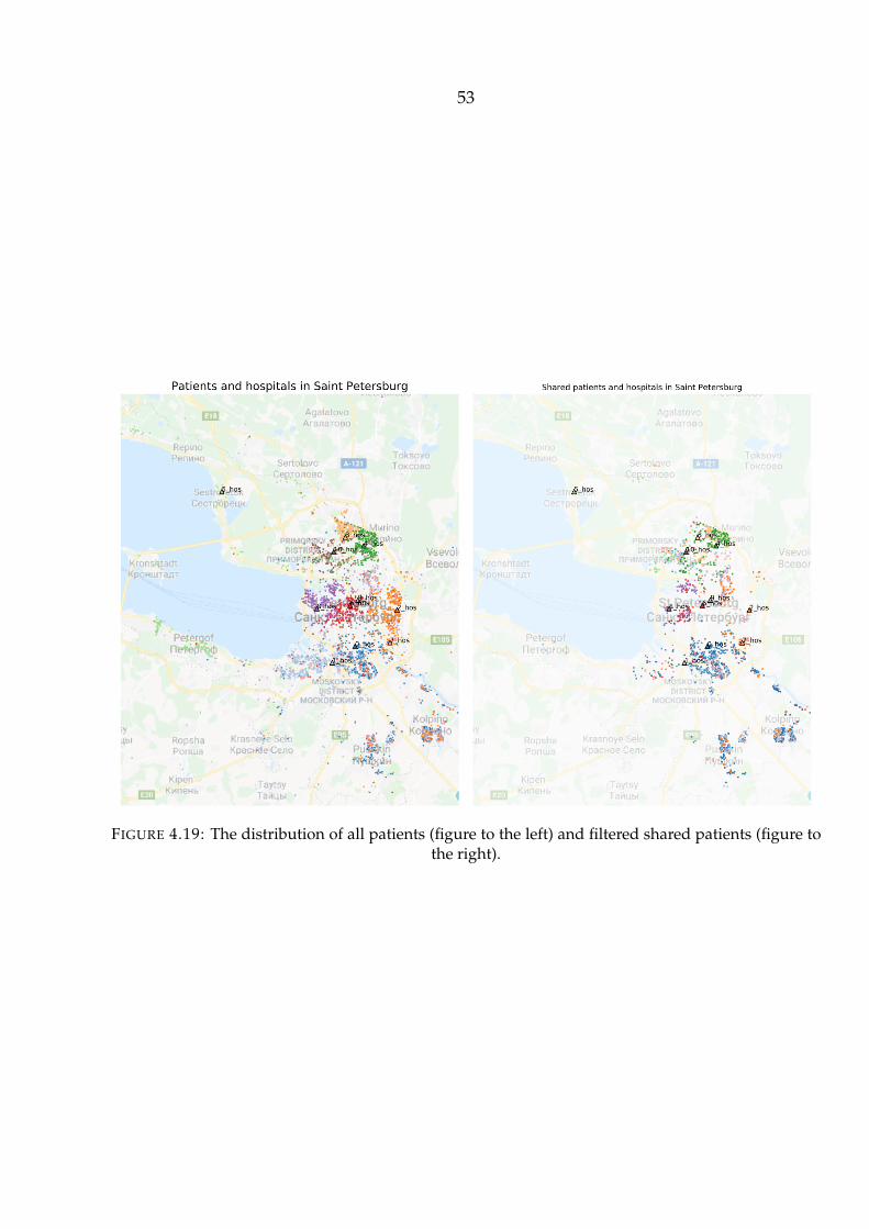
53

FIGURE 4.19: The distribution of all patients (figure to the left) and filtered shared patients (figure tothe right).

54

FIGURE 4.20: The primary actions predicted for all hospitals in Saint Petersburg.

55

TABLE 4.2: Result of the Pearson correlation test for simulated and observed averaged mortality

Strategy combination [’A’, ’A’, ’A’, ’A’, ’A’, ’A’, ’A’, ’A’, ’A’, ’A’](aka "All-Accepting strategies")

Pearson’s r 0.7209P-value 0.0436

Strategy combination [’R’, ’R’, ’R’, ’R’, ’R’, ’R’, ’R’, ’R’, ’R’, ’R’](aka "All-Redirecting strategies")

Pearson’s r 0.8232P-value 0.0064

Strategy combination [’A’, ’R’, ’A’, ’A’, ’R’, ’R’, ’R’, ’A’, ’A’, ’A’](aka "Predicted Strategies")

Pearson’s r 0.7300P-value 0.0256

Thus, the simulated mortality can be estimated by the average door-to-balloon time [34].Figure.4.21 shows the simulated mortality in i_hos for i = 0, 1, 2, 3, 4, 6, 7, 8, 9, 10 by usingpredictive strategies (derived from GT-DES model) is correlated with the observed mortality.However, 0_hos is an exception because 0_hos is a special ACS centre, which behaves dif-ferently from normal hospitals. In addition, since 9_hos is close to 6hos geographically, theGT-DES model is not able to model it accurately because the nearest travelling node to bothof them is the same, so that is occupied by both of them while computing the travelling timeof the simulated patient. Eventually, the lower figures show the mortality simulated by usingpredicted strategies is mostly correlated to the observed mortality.

As a comparative analysis, also to validate the GT-DES model, Table.4.3 shows the Pear-son correlation test is conducted for simulated and real-world mortality in the situation of "AllAccepting", "All Redirecting" and "Predicted Strategies". As the mortality correlation usingpredicted strategies being 0.8232 , the p-value being 0.0064 for a non-correlation test, we re-jected the non-correlation hypothesis by assuming the 1% significant level. The right threefigures in Figure.4.21 shows linear fit of three strategy combinations using least square methodto minimise the error. Besides, Figure.4.22 shows that, by compared with 130 results using dif-ferent combinations of strategy, we fond the strategy combination having the best correlationto the observed mortality is the one predicted by the GT-DES model.

To summarise the ACS case study, at first, we constructed the simulation environmentby transplanted the metropolitan area of Saint Petersburg with locations of 11 hospitals 5124patients. Secondly, we explored the datasets and we found: 1. The geographical distributionof recorded patients is slanted; that is, more patients appeared in the south than the north.Thus, we simulate patient’s requests by random sample from the existed records 2. Due to the

56

FIGURE 4.21: The simulated mortality for recorded hospitals in Saint Petersburg (three figures to theleft) and the correlation between the simulated mortality and observed mortality ( three figures to theright) by using all-accepting strategies, predicted predictive strategies and all-redirecting strategies.It shows the mortality simulated by using predictive strategies is mostly correlated to the observed

mortality.

57

FIGURE 4.22: The Pearson’s r between the observed mortality and simulated mortality by using everypossible strategy combination. Except a0_hos = ”A” a1_hos=”R” a6_hos=”R” are fixed. It shows the mostcorrelated strategy combination is the same to the predicted strategies with Pearson’s being 0.8232.

complex distributions of traffic conjunctions and infrastructures, the travelling time is differentfrom the visual euclidean distance on the map. Thus, we derive the hourly travelling timefrom Yandex.Map and sorted it out properly. 3. Most of the patients request to emergencymedical service between 8 to 23 o’clock, where the timeslot from 10 to 13 o’clock is significantlybusy. Thus, the average request rate is varying hourly according to peak-time effect. 3. Theprobability distribution of serving time is estimated by Kernal density distribution (KDE, anon-parametric estimation) due to the distribution of serving data is an unknown function.

The evaluation of mortality is always challenging for any ambulance dispatching models.Thus, we calculated the average door-to-balloon time for each hospital, which as the primarypayoff, it is strongly correlated to the mortality [42].

As a simulation result for any pair of hospitals, the strategy selection of hospitals matchesour conclusion from stochastic GT-DES model and sensitivity analysis. Furthermore, by ex-tending pair-to-pair simulation to every possible hospital pairs, we rerun and obtained thesimulated mortality for each hospital. We believe the case studied has a practical significancein modelling ambulance-dispatching for acute coronary syndrome patients.

58

5 CONCLUSION AND FUTURE WORK

This thesis has focused on understanding the behaviours of different stakeholders in anambulance-dispatching system (ADS). Specifically, we aimed to clarify the process of patientinflow, the incentive of stakeholders, and the overall pay-off pattern after their complicatedinteraction. Therefore, a queuing-network model was needed to simulate patient inflow (in-cluding sending patient’s request to EMS, deli to the hospital, accepting, redirecting by thehospital and serving and discharging in hospital). What is more, a game-theoretical modelwas needed to predict the hospitals’ actions to patients ("Accepting" or "Redirecting"); wherewe assumed, the hospital is a rational agent and focus on lower mortality as its primary incen-tive. The decision-making process was mainly influenced by the level of patient inflow and theamount of medical resource owned by the hospital and nearby hospitals.

5.1 Conclusion

The main objective of the research project was to simulate and validate the ambulancedispatching of acute coronary syndrome (ACS) patients in a large city (in this thesis, SaintPetersburg was used as an example) by involving real-world data and consultation from localprofessionals.

Traditionally, hospitals would accept a patient without reservation because of their socialresponsibility. However, an initial deterministic simulation for simulating patient inflow byqueuing-network model caught our eyes: "Accepting" action does not always lead to optimumglobal mortality, where "Redirecting" action would result in better global effect when patientinflow reached a certain level. The initial result inspired us to guide hospital to reasonablyredirect patient.

Next, after the verification of the initial experiment by the stochastic queuing-networkmodel, we invoked game theory to analyse the outcome pattern of decision making after as-suming hospitals’ interactions as a non-cooperative game. For which, the internal incentiveand external manifestation of the decision-making process were revealed. The internal incen-tive is that a hospital acts for the sake of a balance between lower mortality and more patients

59

being served by itself. The external manifestation shows hospitals’ strategies formed a Nashequilibrium. Also, we found the strategy selection of a hospital is deliberately slanted as thefollowing: 1. When patient inflow is at a low-level, all hospitals tend to accept patients. 2.Hospital’s strategy transits to "Redirecting" from "Accepting" with the growing level of crowd-edness and transits to "Accepting" back if the whole system is overcrowded. 3. Hospitals withfewer resources (compared to nearby hospitals) tend to switch their strategy preferentially.

The result of the sensitivity analysis provides us with a solid understanding of factor im-portance. 1. Arrival and serving rate are the most and second most important factor for globalmortality. 2. The travelling time is barely affecting the hospital’s strategy selection. 3. Theimportance of capacity of the medical resource owned by a hospital values nearly twice to thehospital’s payoff than the effect resulted by nearby hospitals’ capacity.

Lastly, the properly-validated case study has practical significance in simulating the real-word ambulance-dispatching system. Instead of directly evaluating mortality as the primarypayoff, we simulated the average door-to-balloon time for each hospital, which is strongly cor-related to the mortality. As a result of the local simulation, the behaviour pattern of hospitalsmatches our conclusion from stochastic GT-DES model and sensitivity analysis. Furthermore,by extending pair-to-pair simulation to all available hospitals in Saint Petersburg, we rerun andobtained the simulated mortality of each hospital. To validate the GT-DES model, a compara-tive analysis by comparing simulated and real-world mortality using the Pearson correlationtest is conducted. With the Pearson’s r being 0.8232, the p-value being 0.0064, we reject thenon-correlation hypothesis. Besides, by compared the result of Pearson’s r derived from 130different combinations of strategy, we fond the strategy combination having the best correla-tion to the observed mortality is the one predicted by the GT-DES model.

As supplementary, due to the massive complexity in the health-care system, the proposedGT-DES model was set up as a universal framework. Meaning we put more effort to make themodel more simple, general and extendable. Meanwhile, many experiments’ feasibility andpossible scenarios in realistic were discussed and reasoned with evidence of real-world dataand consultation from local doctors. Although the whole model is thoughtfully based on ahealth-care system in Saint Petersburg, we believe the model can be extended for ambulance-dispatching systems in other cities.

5.2 Possible futurework

This section listed possible work we may go further in the future.

60

The mortality estimation was done by constructing the connection between door-to-balloontime. Further, it is more reliable to construct an improved function where the local factors (e.g.city environment, demographic factors and the capacity of medical resource) are considered[42].

We previously use pair-to-pair simulation to predict the local Nash equilibrium and thencomputed weighted strategies for each hospital. However, it is possible to build and run aglobal simulation entirely. The problem may be the complicated game process (for "Accepting"and "Redirecting" options, the dimension of the payoff matrix would be a 211 = 2048 for elevenhospitals).

The travelling process of patients was estimated by 143 departure nodes and 19 arrivalnodes derived from the map. However, the precision can be improved by coupling with trans-portation models which our colleagues have developed it previously[20].

What is more, the simulated mortality of hospital 0_hos was previously excluded from theresult analysis of ACS case study due to its unique functions (0_hos was a specialised medicalcentre instead of a regular hospital). Thus, a more complicated patient inflow and hospitalregulation shall be taken into account to determine the behaviours of 0_hos and add it to theresult analysis.

In addition, instead of assuming pure Nash equilibrium, a more sophisticated equilibriumcan be assumed, such as the mixed strategies or other complicated GT-approaches.

As the model simulates the ambulance dispatching system, financial and policy-basedregulation can be added and analysed.

In the future, policy-making management can be developed and added to the model,where we can test, verify, compare the different policies to achieve a social optimum of thehealth outcome.

.

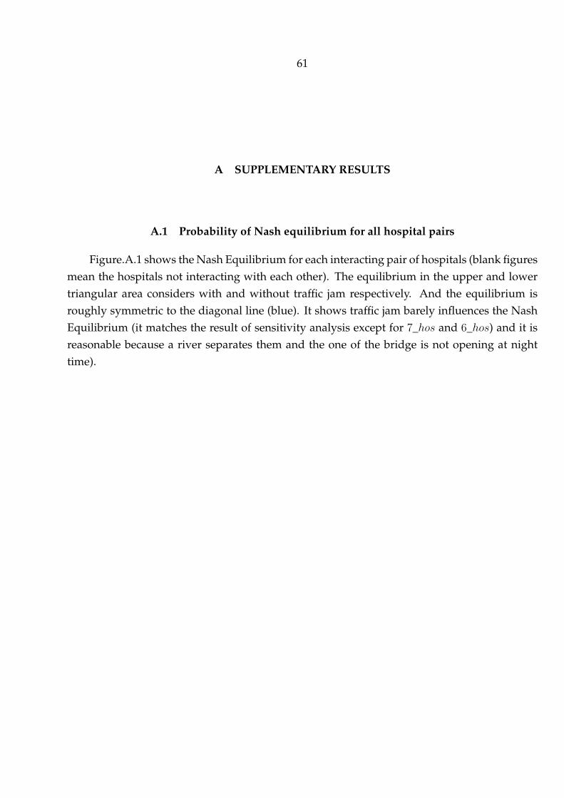
61

A SUPPLEMENTARY RESULTS

A.1 Probability of Nash equilibrium for all hospital pairs

Figure.A.1 shows the Nash Equilibrium for each interacting pair of hospitals (blank figuresmean the hospitals not interacting with each other). The equilibrium in the upper and lowertriangular area considers with and without traffic jam respectively. And the equilibrium isroughly symmetric to the diagonal line (blue). It shows traffic jam barely influences the NashEquilibrium (it matches the result of sensitivity analysis except for 7_hos and 6_hos) and it isreasonable because a river separates them and the one of the bridge is not opening at nighttime).

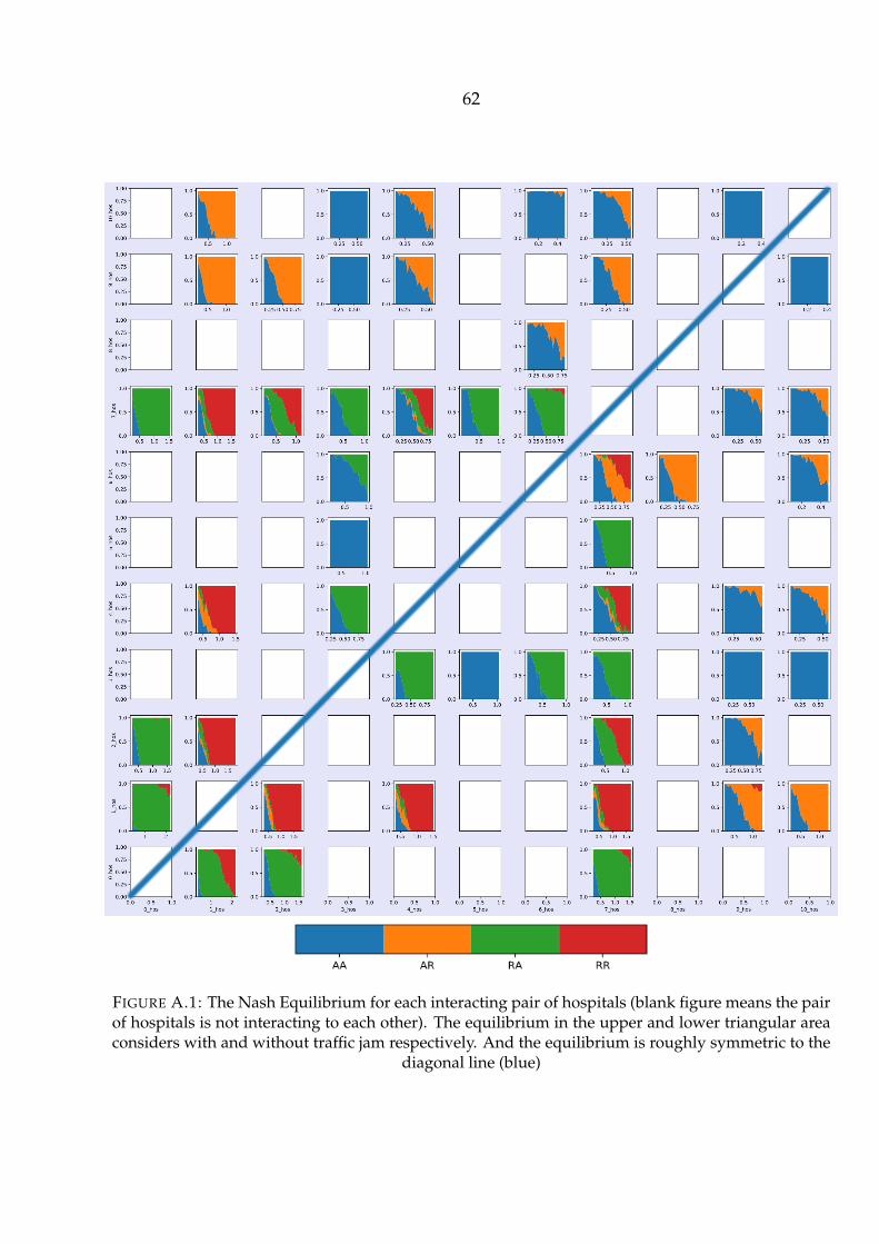
62

FIGURE A.1: The Nash Equilibrium for each interacting pair of hospitals (blank figure means the pairof hospitals is not interacting to each other). The equilibrium in the upper and lower triangular areaconsiders with and without traffic jam respectively. And the equilibrium is roughly symmetric to the

diagonal line (blue)

63

LIST OF FIGURES

1.1 A modelling and simulation life cycle applied to structure a computational model[16] . . . . . . . . . . . . . . . . . . . . . . . . . . . . . . . . . . . . . . . . . . . . . 4

3.1 A flowchart explicitly explains the workflow of the ambulance-dispatching sys-tem (ADS) from the perspectives of stakeholders, including patients, emergencymedical service (EMS) and ED (or hospital). The whole flowchart will be mod-elled by queuing-network model analytically and stochastically except the markedcomment box will be modelled by the game-theoretical model (GTM) to predictthe strategies of EDs or hospitals. . . . . . . . . . . . . . . . . . . . . . . . . . . . . 12

3.2 The figure shows the ambulance-dispatching process on a one-dimensional map.Hj denotes the hospital with unique id j for j = 1, 2, pi denotes the patientwith unique id i, Tc is the distance between H1 and H2 in time. Each Hj has thenumber of Cj server (in realistic, the server is a surgery facility or professionalmedical resource) with serving rate µi patients per hour per server. The queuingbuffer is the waiting room in realistic where patients queue here. A H1 taking"Accepting (A in short)" strategy has the infinite capacity of queuing buffer. H2

taking "Redirecting (R in short)" strategy will redirect the incoming patient toopponent H1 when no vacancy in either its queuing buffer or server. . . . . . . . 14

3.3 The computational structure of a 1-D queuing-network model (QNM) . . . . . . 153.4 A payoff matrix ∈ R2×2×2 for non-cooperative game. N = 1, 2, 3 is a finite

set of three hospital agents. And we define A = A1 × A2 × A3 of action pro-files a = (a1, a2, a3) where aj ∈ Aj = A,R with A as accepting, and R asrejecting/redirecting action where Aj being the set of actions available to agentj. And u = (u1, u2, u3) is a profile of utility function[24]. Thus, hospital j re-ceives the payoff Lj_a = uj(a) and a payoff vector for three hospitals is definedas L = (L1_a, L2_a, L3_a). . . . . . . . . . . . . . . . . . . . . . . . . . . . . . . . . . 21

64

3.5 Simulated two-dimensional area with three hospitals and corresponding capac-ity of servers.Shaded sectors are the "service coverage" zones. Parameters usedareRadius = 40km, origin = (40, 40), and locations of hospitals arePh = [[20.9014, 28.9734], [59.0985, 28.9734], [40, 62.0531]].

. . . . . . . . . . . . . . . . . . . . . . . . . . . . . . . . . . . . . . . . . . . . . . . 233.6 Total-order sensitivity indies of λ with respect to the growing size of distinct

samples N . It shows it shows It shows with the size of distinct samples increaseby logarithmic, the 95% confidence can reach±0.1 atN = 214 (2 significant digitssaved). Analysed by Sobol analysis with 1000-times resembles. . . . . . . . . . . 27

3.7 First and total order sensitivity analysis by setting output as "system score" (topfigure) and the "score of hospital 2" (bottom figure).It shows λ,M contributesmost of the sensitivity to either system or one of hospital’s score. The velocity ofambulance contributes significantly less than other factors. This idea is used inthe later case study where travelling time is not as important as door-to-balloontime (the sum of queuing and serving time). Also, for a specific hospital’s score,we found its capacity and strategy is twice important to its score than them inother hospitals. The distinct sample size N = 214 . . . . . . . . . . . . . . . . . . . 29

4.1 Global time spent at two hospitals of a one-dimensional queuing-network model."A" in the legend stands for accepting strategy, "R" denotes redirecting strategy.The less global time, the better to the system. It shows AA strategy is the mostbeneficial strategy (with dominantly less global time) in most cases, except thecircled interaction in the left figure; where AA switches to RA and RR, and itstarts to reduce the global time when patients flow grows to a certain level, giventhe server N = N1, N2 = [2, 1] is not equal. Parameter used are Tc=6, patientflow is defined as λ

µ1+µ2. . . . . . . . . . . . . . . . . . . . . . . . . . . . . . . . . 30

4.2 A warm-up simulation showing the number of patients served by 3 hospitalsusing different strategy combinations. It shows that when the system is in themiddle-level crowdedness, the "Redirecting" (R) strategy starts being beneficialby serving more patients. The numbers of servers in hospitals are N = [2, 3, 4];so does the queuing lengths; with approximately 400 incoming patients. Foreach gradually added requests, ten simulations were run with random initiali-sation of the patient locations and serving times. The figures are presented bythe means and error bars using one standard deviation. . . . . . . . . . . . . . . . 31

4.3 Contribution of each hospital to the number of total patients served at differentlevels of crowdedness. At the point when the number of patients appeared is230. The figure shows that hospital with four servers contributed most of thepatients served. . . . . . . . . . . . . . . . . . . . . . . . . . . . . . . . . . . . . . . 32

65

4.4 A 2-D working Nash Equilibrium (NE) matrix with outcome argument "Score"as the payoff. given λ = [3, 18],M = [3, 18] in the scenario of N = [2, 2, 2] (left)and N = [2, 1, 2] (right). It shows with growing request rate (λ) and decliningserving rate (M ), the pure Nash Equilibrium transits from AAA to RRR untilthe system is inconsistent. The term "inconsistent" (abbr. "Incon Sys", shownas grey square in the plot) states there is no NE due to the system being over-crowded (meaning queuing time goes to infinite in EACH hospital for incomingpatients). Each block shows the most frequent Nash Equilibrium among all 106realisations The area of a coloured inner square divided by 1 is the probability ofoccurrences (i.e. the probability of AAA strategy being NE at the left-top corneris 100%). And each NE is searched from payoff matrix 3.4 by algorithm 1, Simu-lation parameters used are: 106 simulations for each block (20× 20 = 400 rectan-gles in total), simulation time ranges from 30 to 135hours, the appeared numberof patients ranges from 400 to 2500, vamb = 50km/hour, hi.maxQueue = [2, 2, 2] . . 34

4.5 An arbitrary example of the dispersive distribution for the occurrence of NashEquilibrium in a simulation. In this case, the RRR strategy is selected as NashEquilibrium due to RRR appeared 17.92% in 106 simulations. . . . . . . . . . . . 35

4.6 An example showing the time consumption when λ = 7.73, µ = 13.26. It showsthe time consumption for each patient given AAA (top figure) and RRR (botfigure) strategy. It shows RRR has averagely less queuing time due to havingless peak-time effect (peak-time timeslots are marked in red) . . . . . . . . . . . . 37

4.7 A 2-D working Nash Equilibrium (NE) matrix with outcome argument "Score"as payoff. given λ = [3, 18],M = [3, 18] in the scenario of N = [2, 3, 2] andN = [1, 2, 3] . It shows with growing request rate λ and declining serving rateM , the pure Nash Equilibrium transits from AAA ⇒ RAR ⇒ RRR ⇒ ARR &

RRA⇒ inconsistent. . . . . . . . . . . . . . . . . . . . . . . . . . . . . . . . . . . . 384.8 Eleven hospitals having angiography in Saint Petersburg (using index instead

of real hospital names). Hospitals work 24/7 and 5124 patients going to each ofthem. Background map is derived from Google Map application. The scale ofmap is 1km : 1, and 1 yard of latitude equals 111.111km on real world. . . . . . . 42

4.9 Patient selected for local simulation in an isolated rectangular area . . . . . . . . 434.10 Plotted histogram for Tinterval of patients’ requests from our data (5124 records

of ACS patients made calls to EMS). Figure shows the time interval of patientsappearances can be fitted by exponential distribution with λ = 0.6911, meaningthe average of interval between ACS patient’s request is 1

λ≈ 1.4470 hours both

4 digits saved. . . . . . . . . . . . . . . . . . . . . . . . . . . . . . . . . . . . . . . . 43

66

4.11 The average number of requests per hour in a day to Almazov medical centrefrom 01/01/2015 to 15/11/2015. It shows the request rate changes hourly in aday: the rush hour of receiving request is roughly at around noon. And at 6 am,there will be fewer requests on average. . . . . . . . . . . . . . . . . . . . . . . . . 44

4.12 Travelling network containing 143 departure nodes and 19 destination nodesincluding 13 hospitals as destination . . . . . . . . . . . . . . . . . . . . . . . . . . 45

4.13 The average travelling time hourly for all the available connections. The plotshows time period at around 9 am or between 6 pm, and 7 pm are the rush hourslots in Saint Petersburg. The data is normalised to [0, 1]. One standard deviationused as error bar above and below mean value. . . . . . . . . . . . . . . . . . . . . 46

4.14 Demonstration of stent time after removing outliers (stentT ime > threshold =

400 and stentT ime 0. . . . . . . . . . . . . . . . . . . . . . . . . . . . . . . . . . 474.15 Experimental fits of the stent time data (left). A comparison of the cumulative

random variable of stent time and cumulative density plot of data simulated bythe KDE method . . . . . . . . . . . . . . . . . . . . . . . . . . . . . . . . . . . . . 48

4.16 The probability of Nash Equilibrium for 0_hos and 1_hos (left) and reverse (right)with respect to patient inflow. The range of patient inflow is partitioned betweenmax and min arrival rate of isolated patients in a day. 30 realisations for each pa-tient inflow and 7200 hours simulation time for each realisation. Also, 0_hos hasfacility0 = 2 and 1_hos has facility1 = 1 and the serving rate is 1.15 patientper hour per server. Traffic jam is considered only for the top two figures. Thehospital with fewer servers 1_hos switches strategy first. . . . . . . . . . . . . . . 50

4.17 The probability of different Nash Equilibrium with respect to patient inflow for10_hos and 3_hos . . . . . . . . . . . . . . . . . . . . . . . . . . . . . . . . . . . . . 51

4.18 The heat map shows the proportion of the shared patients for every hospital pair. 524.19 The distribution of all patients (figure to the left) and filtered shared patients

(figure to the right). . . . . . . . . . . . . . . . . . . . . . . . . . . . . . . . . . . . 534.20 The primary actions predicted for all hospitals in Saint Petersburg. . . . . . . . . 544.21 The simulated mortality for recorded hospitals in Saint Petersburg (three figures

to the left) and the correlation between the simulated mortality and observedmortality ( three figures to the right) by using all-accepting strategies, predictedpredictive strategies and all-redirecting strategies. It shows the mortality simu-lated by using predictive strategies is mostly correlated to the observed mortality. 56

4.22 The Pearson’s r between the observed mortality and simulated mortality by us-ing every possible strategy combination. Except a0_hos = ”A” a1_hos=”R” a6_hos=”R”

are fixed. It shows the most correlated strategy combination is the same to thepredicted strategies with Pearson’s being 0.8232. . . . . . . . . . . . . . . . . . . . 57

67

A.1 The Nash Equilibrium for each interacting pair of hospitals (blank figure meansthe pair of hospitals is not interacting to each other). The equilibrium in theupper and lower triangular area considers with and without traffic jam respec-tively. And the equilibrium is roughly symmetric to the diagonal line (blue) . . . 62

68

LIST OF TABLES

3.1 Table of General Notations in Numerical Model . . . . . . . . . . . . . . . . . . . 223.2 Table of Attribute Notations of Agent: Patient . . . . . . . . . . . . . . . . . . . . . 243.3 Table of Attribute Notations of Agent: Hospital . . . . . . . . . . . . . . . . . . . . 243.4 SA indices of λ w.r.t sample size . . . . . . . . . . . . . . . . . . . . . . . . . . . . . 27

4.1 Definition and values of input variables in the computational GT-DES model . . 334.2 Result of the Pearson correlation test for simulated and observed averaged mor-

tality . . . . . . . . . . . . . . . . . . . . . . . . . . . . . . . . . . . . . . . . . . . . 55

69

REFERENCE

[1] Mark D Agee and Zane Gates. “Lessons from game theory about healthcare system priceinflation”. In: Applied health economics and health policy 11.1 (2013), pp. 45–51.

[2] Ezra A Amsterdam et al. “2014 AHA/ACC guideline for the management of patientswith non–ST-elevation acute coronary syndromes: a report of the American College ofCardiology/American Heart Association Task Force on Practice Guidelines”. In: Journalof the American College of Cardiology 64.24 (2014), e139–e228.

[3] Tobias Andersson and Peter Värbrand. “Decision support tools for ambulance dispatchand relocation”. In: Journal of the Operational Research Society 58.2 (2007), pp. 195–201.

[4] Jerry Banks et al. Discrete-event system simulation. Pearson, 2005.[5] Valérie Bélanger, A Ruiz, and Patrick Soriano. “Recent optimization models and trends in

location, relocation, and dispatching of emergency medical vehicles”. In: European Journalof Operational Research 272.1 (2019), pp. 1–23.

[6] Lloyd G Connelly and Aaron E Bair. “Discrete event simulation of emergency depart-ment activity: A platform for system-level operations research”. In: Academic EmergencyMedicine 11.11 (2004), pp. 1177–1185.

[7] Richard A Davis, Keh-Shin Lii, and Dimitris N Politis. “Remarks on some nonparametricestimates of a density function”. In: Selected Works of Murray Rosenblatt. Springer, 2011,pp. 95–100.

[8] Sarang Deo and Itai Gurvich. “Centralized vs. decentralized ambulance diversion: A net-work perspective”. In: Management Science 57.7 (2011), pp. 1300–1319.

[9] George A. Diamond, Alan Rozanski, and Michael Steuer. “Playing doctor: Applicationof game theory to medical decision-making”. In: Journal of Chronic Diseases 39.9 (1986),pp. 669 –677. ISSN: 0021-9681. DOI: https://doi.org/10.1016/0021-9681(86)90148-7. URL: http://www.sciencedirect.com/science/article/pii/0021968186901487.

[10] Wolfgang F Dick. “Anglo-American vs. Franco-German emergency medical services sys-tem”. In: Prehospital and disaster medicine 18.1 (2003), pp. 29–37.

[11] “Effects of increasing the number of players and memory size in the iterated Prisoner’sDilemma: a numerical approach”. In: Proceedings of the Royal Society B: Biological Sciences

70

264.1381 (1997), pp. 513–519. ISSN: 0962-8452. DOI: 10.1098/rspb.1997.0073. URL:http://rspb.royalsocietypublishing.org/cgi/doi/10.1098/rspb.

1997.0073.[12] Xinyu Fu et al. “Coupling Game Theory and Discrete-Event Simulation for Model-Based

Ambulance Dispatching”. In: Procedia Computer Science 136 (2018), pp. 398–407.[13] Jeffrey Goldberg et al. “A simulation model for evaluating a set of emergency vehicle

base locations: Development, validation, and usage”. In: Socio-economic planning sciences24.2 (1990), pp. 125–141.

[14] Reidar Hagtvedt et al. “Cooperative strategies to reduce ambulance diversion”. In: (2009),pp. 1861–1874.

[15] Jonathan D Herman and Will Usher. “SALib: An open-source Python library for Sensi-tivity Analysis.” In: J. Open Source Software 2.9 (2017), p. 97.

[16] Alfons G Hoekstra et al. “Multiscale computing for science and engineering in the era ofexascale performance”. In: Philosophical Transactions of the Royal Society A 377.2142 (2019),p. 20180144.

[17] Keisuke Inakawa, Takehiro Furuta, and Atsuo Suzuki. “Effect of ambulance station lo-cations and number of ambulances to the quality of the emergency service”. In: TheNinth International Symposium on Operations Research and Its Applications (ISORA’10). 2010,pp. 340–347.

[18] Zied Jemai, L Aboueljinane, E Sahin, et al. A review on simulation models applied to emer-gency medical service operations. Tech. rep. 2013.

[19] Charlotte Kelly et al. “Are differences in travel time or distance to healthcare for adultsin global north countries associated with an impact on health outcomes? A systematicreview”. In: BMJ open 6.11 (2016), e013059.

[20] Konstantin Knyazkov et al. “Evaluation of dynamic ambulance routing for the trans-portation of patients with acute coronary syndrome in Saint-Petersburg”. In: ProcediaComputer Science 66 (2015), pp. 419–428.

[21] Sergey V Kovalchuk, Mariia A Moskalenko, and Alexey N Yakovlev. “Towards model-based policy elaboration on city scale using game theory: application to ambulance dis-patching”. In: International Conference on Computational Science. Springer. 2018, pp. 404–417.

[22] BV Gnedenko Igor Nikolaevich Kovalenko. Introduction to queueing theory. Israel Programfor Scientific Translation, Jerusalem, 1968.

[23] Taesik Lee et al. “A simulation-based iterative method for a trauma center—Air ambu-lance location problem”. In: Proceedings of the 2012 Winter Simulation Conference (WSC).IEEE. 2012, pp. 1–12.

71

[24] Kevin Leyton-Brown and Yoav Shoham. “Essentials of game theory: A concise multidis-ciplinary introduction”. In: Synthesis lectures on artificial intelligence and machine learning2.1 (2008), pp. 1–88.

[25] Cheng Siong Lim, Rosbi Mamat, and Thomas Braunl. “Impact of ambulance dispatchpolicies on performance of emergency medical services”. In: IEEE Transactions on Intelli-gent Transportation Systems 12.2 (2011), pp. 624–632.

[26] Kyle Y Lin. “Decentralized admission control of a queueing system: A game-theoreticmodel”. In: Naval Research Logistics (NRL) 50.7 (2003), pp. 702–718.

[27] Norm Matloff. “Introduction to discrete-event simulation and the simpy language”. In:Davis, CA. Dept of Computer Science. University of California at Davis. Retrieved on August2.2009 (2008), pp. 1–33.

[28] J McCarter. Office of the Auditor General of Ontario, 2010 Annual Report. 2010.[29] Natasha Mihal and Renee Moilanen. “When emergency rooms close: Ambulance diver-

sion in the West San Fernando Valley”. In: (2005).[30] Debra K. Moser et al. “Reducing Delay in Seeking Treatment by Patients With Acute

Coronary Syndrome and Stroke”. In: The Journal of Cardiovascular Nursing 22.4 (2007),pp. 326–343. ISSN: 0889-4655. DOI: 10 . 1097 / 01 . JCN . 0000278963 . 28619 . 4a.URL: http://content.wkhealth.com/linkback/openurl?sid=WKPTLP:landingpage\&an=00005082-200707000-00013.

[31] Farzad Mostashari et al. “Use of ambulance dispatch data as an early warning systemfor communitywide influenzalike illness, New York City”. In: Journal of Urban Health80.1 (2003), pp. i43–i49.

[32] Roger B Myerson. Game theory. Harvard university press, 2013.[33] Maribeth Hughett Price. Mastering ArcGIS. McGraw-Hill, 2010.[34] Saif S Rathore et al. “Association of door-to-balloon time and mortality in patients admit-

ted to hospital with ST elevation myocardial infarction: national cohort study”. In: Bmj338 (2009), b1807.

[35] George P Richardson, Alexander L Pugh, et al. Introduction to system dynamics modelingwith DYNAMO. Vol. 48. MIT press Cambridge, MA, 1981.

[36] Jennifer Prah Ruger, Lawrence M Lewis, and Christopher J Richter. “Patterns and factorsassociated with intensive use of ED services: implications for allocating resources”. In:The American journal of emergency medicine 30.9 (2012), pp. 1884–1894.

[37] James Rumbaugh et al. Object-oriented modeling and design. Vol. 199. 1. Prentice-hall En-glewood Cliffs, NJ, 1991.

[38] Andrea Saltelli et al. Global sensitivity analysis: the primer. John Wiley & Sons, 2008.[39] Andrea Saltelli et al. “Sensitivity analysis in practice: a guide to assessing scientific mod-

els”. In: Chichester, England (2004).

72

[40] Martin Shubik. Game theory in the social sciences: concepts and solutions. Vol. 155. MIT pressCambridge, MA, 1982.

[41] Pedro Marinho Sizenando Silva and Luiz Ricardo Pinto. “Emergency medical systemsanalysis by simulation and optimization”. In: Proceedings of the 2010 winter simulationconference. IEEE. 2010, pp. 2422–2432.

[42] CY Soon, WX Chan, and HC Tan. “The impact of time-to-balloon on outcomes in patientsundergoing modern primary angioplasty for acute myocardial infarction”. In: Singaporemedical journal 48.2 (2007), p. 131.

[43] Xu Sun. “Modeling the Emergency Care Delivery”. In: (2014).[44] C Tarrant, T Stokes, and A M Colman. “Models of the medical consultation: opportuni-

ties and limitations of a game theory perspective”. In: BMJ Quality & Safety 13.6 (2004),pp. 461–466. ISSN: 1475-3898. DOI: 10.1136/qshc.2003.008417. eprint: https://qualitysafety.bmj.com/content/13/6/461.full.pdf. URL: https://qualitysafety.bmj.com/content/13/6/461.

[45] Terje Totland. “5.2. 7 Object Modeling Technique (OMT) Thesis”. In: Norwegian Universityof Science and Technology (NTNU), Trondheim (1997).

[46] Rhema Vaithianathan. “Health insurance and imperfect competition in the health caremarket”. In: Journal of health economics 25.6 (2006), pp. 1193–1202.

[47] Martin Van Buuren et al. “Evaluating dynamic dispatch strategies for emergency medicalservices: TIFAR simulation tool”. In: Proceedings of the 2012 Winter Simulation Conference(WSC). IEEE. 2012, pp. 1–12.

[48] Joel Watson. Strategy: an introduction to game theory. Vol. 139. WW Norton New York, 2002.