Department of Chemical and Biological Engineering

CHALMERS UNIVERSITY OF TECHNOLOGY

Gothenburg, Sweden 2014

Coupling dense and dilute granular flows in a high shear Mi-Pro granulator Master’s Thesis within the Innovative and Sustainable Chemical Engineering programme

EVA MARÍA GÓMEZ FINO

ABSTRACT

A multi regime system has been modelled in a high-shear MiPro granulator using the Eulerian-

Eulerian framework. The rheology of the granular material has been studied applying Kinetic

Theory of Granular Flow (KTGF) for dilute regimes and a rheology model for dense regimes (Jop

et al., 2006). Experimens were conducted to validate and study the accuracy of the model. The

velocity profiles were successfully obtained using a high speed camera and PIV analysis. In

general, the highest values of both tangential and axial velocity were found in the region

neighboring the impeller blades, showing that the velocity distribution depends on the impeller

position. The partial slip conditions at the boundaries of the system were also evaluated based

on experimental data. An over–prediction of the velocity was found; however, the model has

shown an improvement making it a good replacement for Schaeffer’s extension of KTGF in

dense regimes.

v

ACKNOWLEDGMENTS

To Anders Rasmuson, for giving me the opportunity to work in the department. To

Mohammad Khalilitehrani, for his dedication and guidance during this project. To my family, for

their infinite love and unconditional support. To my friends, for their company and all the good

times. To Gunnar.

vi

TABLE OF CONTENT

INTRODUCTION ................................................................................................................................................. 10

High shear granulation .................................................................................................................................... 11

General objective ............................................................................................................................................. 12

Outline ............................................................................................................................................................. 12

CHAPTER 1 ......................................................................................................................................................... 13

THEORY ................................................................................................................................................................. 13

1.1 Granular flow regimes ............................................................................................................................... 13

1.2 Continuum modelling of granular flow ...................................................................................................... 15

1.3 Rheology model ......................................................................................................................................... 18

1.4 Solids pressure ........................................................................................................................................... 20

CHAPTER 2 ......................................................................................................................................................... 22

EXPERIMENTAL WORK .......................................................................................................................................... 22

2.1 Materials and equipment .......................................................................................................................... 22

2.2 High Speed Imaging ................................................................................................................................... 23

2.3 Particle Image Velocimetry ........................................................................................................................ 24

2.4 Data post-processing ................................................................................................................................. 25

CHAPTER 3 ......................................................................................................................................................... 26

NUMERICAL MODELLING ..................................................................................................................................... 26

3.1 Mesh and geometry ................................................................................................................................... 26

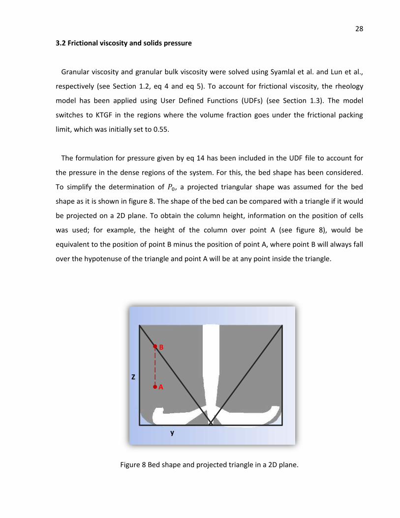
3.2 Frictional viscosity and solids pressure ...................................................................................................... 28

3.3 Boundary conditions .................................................................................................................................. 29

CHAPTER 4 ......................................................................................................................................................... 30

RESULTS AND DISCUSSION ................................................................................................................................... 30

4.1 Visual observations .................................................................................................................................... 31

4.2 Velocity profiles (PIV) ................................................................................................................................. 31

4.3 Numerical model........................................................................................................................................ 36

CONCLUSIONS ................................................................................................................................................... 41

REFERENCES ...................................................................................................................................................... 42

vii

FIGURE INDEX

Figure 1 Schematic view of a Mi-Pro high shear granulator. .........................................................11

Figure 2 Flow regimes of granular material. ..................................................................................14

Figure 3 Separation of scales in multiphase flow. ..........................................................................16

Figure 4 Friction coefficient as a function of inertial number. Inset: definition of pressure, shear

stress and shear rate. (P Jop et al., 2006) ......................................................................................19

Figure 5 Pro-C-epT high shear granulator. .....................................................................................23

Figure 6 Schematic view of experimental setup. ...........................................................................24

Figure 7 Computational mesh of the two sub-domains. (a) Stationary domain: upper view, (b)

stationary domain: side view, (c) rotating domain: upper view, (d) rotating domain: side view.

(Darelius et al., 2008) .................................................................................................................... 27

Figure 8 Bed shape and projected triangle in a 2D plane. .............................................................28

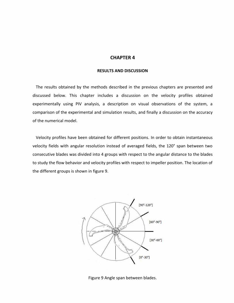
Figure 9 Angle span between blades. .............................................................................................30

Figure 10 Velocity profiles for the three blade passes of one revolution. .....................................32

Figure 11 Averaged velocity profiles experimentally obtained. ....................................................33

Figure 12 Axial velocity profiles with respect to impeller position: (a) from experimental, (b)

from simulation. ............................................................................................................................ 34

Figure 13 Tangential velocity profiles with respect to impeller position: (a) from experimental,

(b) from simulation. ........................................................................................................................35

Figure 14 Histogram over volume fraction distribution in the interior of the vessel. ...................36

Figure 15 Comparison between experimental and simulation results. .........................................37

Figure 16 Contour of volume fraction in the interior of the granulator: dense regions. (a) Side

view, (b) top view, (c) bottom view................................................................................................38

Figure 17 Average volume fraction on the walls of the vessel. .....................................................39

viii

LIST OF SYMBOLS AND ABBREVIATIONS

Latin symbols

Particle diameter

Coefficient of restitution

Constant

Gravity

Radial distribution function

Inertial number

Constant function of particle material and size

Fitting parameter function of particle material, size and shape

Constant

Constant

Confining pressure

Granular pressure

Constant

Particle velocity

Greek symbols

Particle volume fraction

Interphase momentum transfer coefficient

Constant related to quality of the particles

Shear rate

Effective viscosity

Average angle of inclined surface

Granular temperature

Friction coefficient

ix

Particle density

Shear stress

Gas-phase shear stress

Solid-phase shear stress

Abbreviations

CFD Computational Fluid Dynamics

DEM Discrete Element Method

HSI High Speed Imaging

KTGF Kinetic Theory of Granular Flow

PIV Particle Image Velocimetry

UDF User Defined Function

INTRODUCTION

Granulation in high shear mixers is an important unit operation often used in the development

and manufacturing of tablets in the pharmaceutical industry. The study of granulation requires

an understanding of the complex behavior of granular flows. Handling granular materials is also

important in many other industries including food and agricultural industry, mineral processing,

detergents and chemicals (Iveson et al., 2001).

The behavior of granular materials is complex and a complete understanding does not exist

even for simple systems. It displays a varying behavior and it can be considered to be a solid in

a resting state, it can flow as a liquid or behave as a gas when strongly agitated (Jaeger, Nagel, &

Behringer, 1996). For the two extreme regimes, constitutive equations have been proposed

based on kinetic theory for collisional rapid flows, and soil mechanics for slow plastic flows. The

granulation process generally includes multi-regime flow, which means that both dilute and

dense regimes are present. Dilute or rapid granular flows can be modelled using the Kinetic

Theory of Granular Flow (KTGF). However, there is no well-defined theory that described the

dense granular flows because it shows a combination of fluid and solid characteristics (Jop et al.,

2006).

Computational fluid dynamics (CFD) is an emerging technique for predicting the flow behavior

of fluid systems, as it is necessary for scale-up, design, or optimization. Although single-phase

flow CFD models are widely and successfully applied, multiphase CFD is not as simple due to the

difficulty in describing the variety of interactions in these systems. CFD models for multiphase

systems can be divided into two categories: Lagrangian or discrete particle models, and Eulerian

models. The Discrete Element Method (DEM) in which the motion of every single particle and its

interactions with other particles are tracked, is the most conventional and straightforward

approach to modelling particulate systems in mixers. However, it involves a considerable

amount of computational power and it cannot treat more than a million particles (Darelius et

al., 2008), for this reason it becomes unfeasible when studying industrial-size granulation with

billions of particles. Another approach for modelling multiphase flows is the Eularian-Eularian

11

approach where particles are not followed individually, but instead are treated as continua with

properties derived from closure models. The continuum approach drastically decreases

computational power demand having the potential to model industrial-scale granulators, but

potentially misses details about the individual particles (Darelius, 2008).

A recent model framework for dealing with steady dense granular flows have been proposed

(Jop et al., 2006), in which the intermediate regime is described as a visco-plastic fluid based on

the fact that granular liquids shows yield criterion and a complex dependence between shear

stress and shear rate (Khalilitehrani et al., 2013).

High shear granulation

High shear granulation has been one of the most commonly used methods to produce

granules since early 1980s (Parikh, 1997). Most of the high-shear granulators consist of a mixing

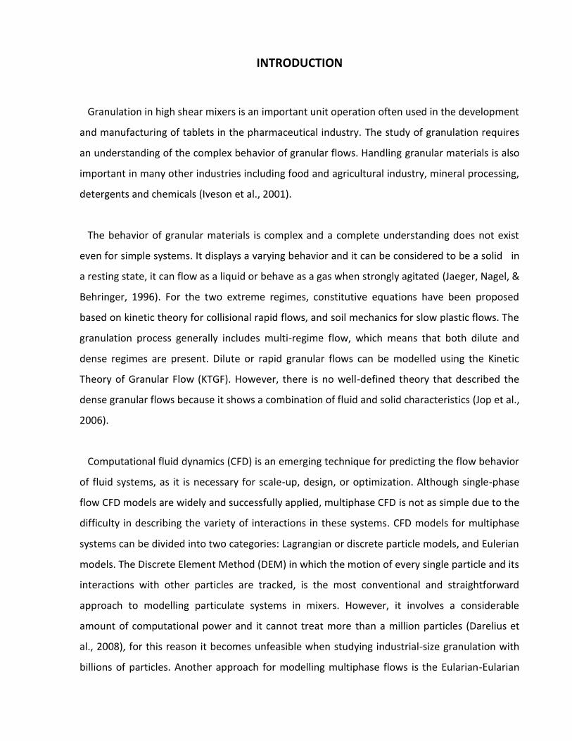
bowl, a three-bladed impeller and an auxiliary chopper to break down the wet mass to produce

granules. Figure 1 shows a schematic view of a Mi-Pro high shear granulator.

Figure 1 Schematic view of a Mi-Pro high shear granulator.

The granulation process includes three different steps: dry mixing, liquid adding and wet

granulation. During the first step, the ingredients are mixed until a homogenous dry mixture is

12

obtained. In the liquid addition stage, a binder liquid is added to the mixture. Once the liquid is

absorbed onto the surface of the powder entities, nucleation starts, particles begin to

agglomerate and grow, and large agglomerates break apart to smaller entities (Darelius et al.,

2010). These simultaneous phenomena make the physics of this part of the process extremely

complex. The last stage of the process is the wet massing. In this stage, several characteristics of

the process are set in a way that gives favorable properties such as size range and level of

compactness. These parameters include process time, chopper and impeller speed, and the

ratio of powder to liquid content. Through this step of the process, particles grow in size and

their liquid content is encapsulated into the structure of the produced entities (Litster, 2003).

General objective

The aim of this study is to model a high shear Mi-Pro granulator that includes both dilute and

dense regimes using the Eulerian-Eulerian framework and study the rheology of granular

material using recent theory for dense particulate flows (Jop et al., 2006). The partial slip

condition at the boundaries of the system is also evaluated based on experimental data.

Velocity profiles from experimental results and simulations will be finally compared to validate

and study the accuracy of the model in both micro- and macro-scale.

Outline

The first chapter of this thesis provides an understanding on the theory of granular flow,

especially on dense particulate flows, and a summary of the most important statements on the

rheology model used for this project. In Chapter 2 there is a detailed description of the

experimental work. A description of the materials and the equipment is included as well as the

techniques used and post-processing procedures. Chapter 3 gives an explanation on the

numerical modelling of the flow, solution strategy and convergence. The results and discussion

on both the experimental work and simulations are found in Chapter 4 to finalize with a set of

conclusions and recommendations for future work.

CHAPTER 1

THEORY

This chapter is indented to provide an understanding of the theoretical basis that constitute

the foundation for this research. The behavior of granular flows, followed by a detailed

description of the continuum modeling of granular flow and the rheology model are presented

in the following sections.

Granular materials are large assemblies of discrete macroscopic particles. If the grains are

large enough (dp > 250µm) and they are surrounded by low viscosity fluid, such as air, the

particle interactions are dominated by contact interactions (Midi, 2004). Capillary forces, van

der Waals forces or viscous interaction can be neglected and the mechanical properties of the

material are only controlled by the momentum transfer during collision or frictional contacts

between grains (Midi, 2004). However, granular material behaves differently from any other

familiar form of matter and is not easy to describe (Jaeger et al., 1996).

1.1 Granular flow regimes

Depending on the local volume fraction and degree of excitation (e.g. flow velocity), granular

flows can be divided in three different categories: granular solids, liquids and gases (Jaeger et

al., 1996). Figure 2 shows the transition between the different flow regimes for granular

materials.

For dilute regimes, when the particles are widely spaced and the system is strongly agitated,

granular flows exhibit gas-like behavior in which the flow is largely governed by the random

movement and collisions between particles; the contact between the particles are of short

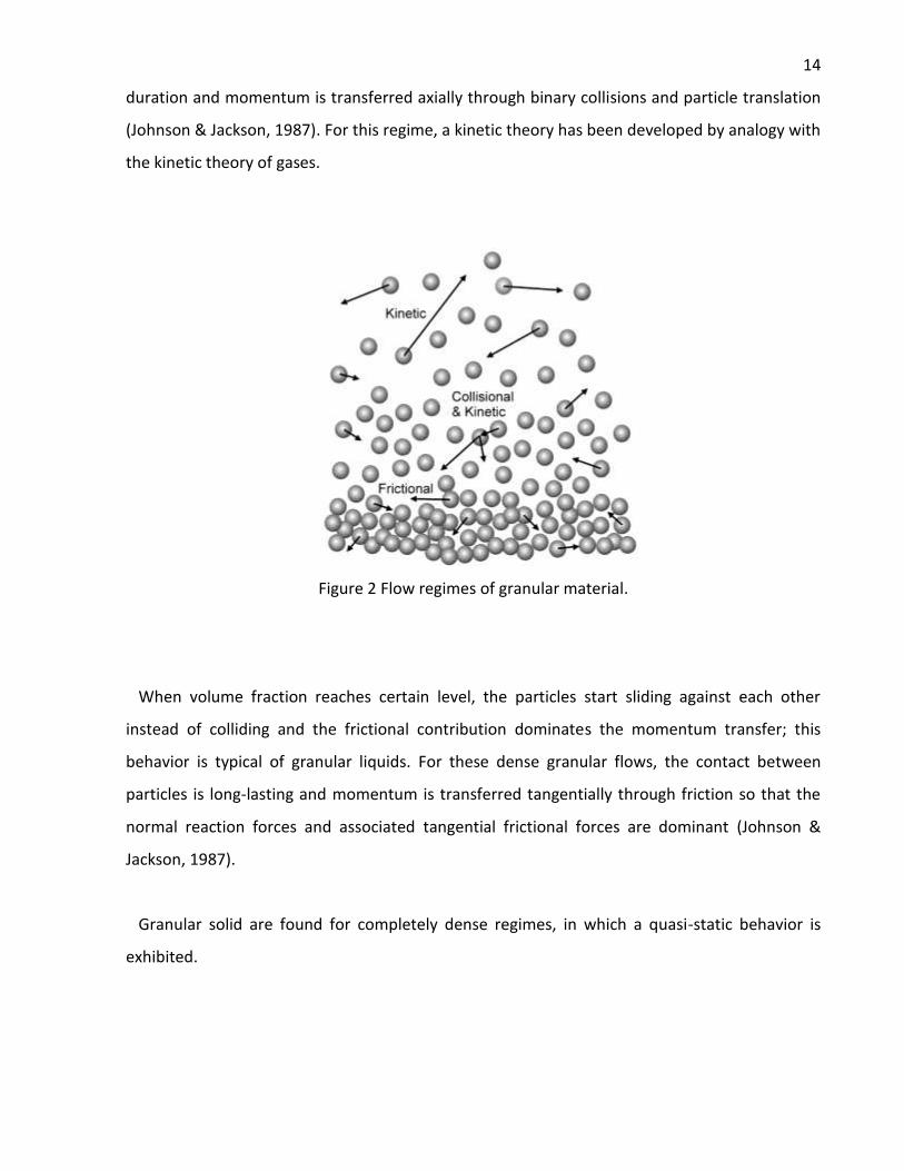
14

duration and momentum is transferred axially through binary collisions and particle translation

(Johnson & Jackson, 1987). For this regime, a kinetic theory has been developed by analogy with

the kinetic theory of gases.

Figure 2 Flow regimes of granular material.

When volume fraction reaches certain level, the particles start sliding against each other

instead of colliding and the frictional contribution dominates the momentum transfer; this

behavior is typical of granular liquids. For these dense granular flows, the contact between

particles is long-lasting and momentum is transferred tangentially through friction so that the

normal reaction forces and associated tangential frictional forces are dominant (Johnson &

Jackson, 1987).

Granular solid are found for completely dense regimes, in which a quasi-static behavior is

exhibited.

15

1.2 Continuum modelling of granular flow

In Eulerian models, the particle phase is treated as a continuum and the motion on the scale

of individual particles is averaged, thus making it possible to treat dense-phase flows in

simulations and study systems of industrial size. As a result, CFD modeling based on this

Eulerian framework is still the only feasible approach for performing parametric investigation

and scale-up and design studies (van Wachem et al., 2001).

The continuum approach for modelling multiphase flows have been developed using the

kinetic theory approach accredited to Bagnold (1954) who derived an equation for particle

pressure. In 1980, Ogawa et al. (1980) formulated an equation for the kinetic energy produced

by shear to emphasize the importance of particle motion. Savage and Jeffrey (1981) noted the

equivalence of the random particle motion to the classical molecular motion and initiated the

kinetic theory approach, and was later complemented by others (Jenkins and Savage, 1983; Lun

et al., 1984; Johnson and Jackson, 1987). In this continuum description particles are not

followed individually, but instead are treated as a continuous medium with properties derived

from closure models, decreasing the demand of computational power and making it suitable for

systems with a large number of particles (Darelius et al., 2008).

The most common used governing equations are those derived by Jackson (1997) which

represent momentum balances for the fluid and solid phases. Jackson used a definition of local

mean variables and the Newton´s equation of motion for a single particle to translate the point

Navier-Stoke equations for the fluid directly into continuum equations. The point variables are

averaged over regions that are large with respect to the particle diameter (microscopic), but

small with respect to the characteristic dimension of the system (macroscopic). Several studies

have shown success in applying continuum models of granular flows. But the approach is also

debated. The averaging procedure used in forming the equations demand that there is a

separation between the microscopic particle scale and the macroscopic flow scale (see figure 3).

16

Figure 3 Separation of scales in multiphase flow.

The continuity and momentum equations derived by Jackson (1997) are given in eq 1 and eq

2, as reported by van Wachem et al. (2001).

(1)

[

] ( ) (2)

where, is the particle velocity and is the particle density, is the solids or granular

pressure and is the shear stress. The first two terms on the right-hand side represent the

forces exerted on particles by the fluid, the next two terms represent the force due to solid-

solid contacts, which can be described using concepts of kinetic theory, followed by the phase

exchange term and the effect of gravity forces on the particles.

The closure of the solid-phase momentum equation requires a description of the solid-phase

stress. For dilute regimes, when the motion is dominated by the particle streaming and

Macroscopic

Microscopic

Plateau

Averaging interval

Ave

rage

d v

alu

e

17

collisional interactions, the effective stress tensor can be described using the kinetic theory of

gases. The model has been previously used in granulators, but has shown deficiencies especially

in the dense regions. The extension of KTGF to dense regions was proposed by Schaeffer, (1987)

and Johnson & Jackson, (1987). The failures of this approach may be explained by the

characteristics of the frictional stress model. Based on this approach, the solid phase stresses

are determined by combination of kinetic, collisional and frictional contributions so that the

frictional stresses are just added to the stress field (see eq 3).

∑ (3)

To account for the shear viscosity due to kinetic motion the expression shown in eq 4 from

Syamlal et al., (1993) is available. On the other hand, the solids bulk viscosity, which accounts

for the resistance of the granular particles to compression and expansion, has the form from

Lun et al., (1984) that is shown in eq 5.

√

[

] (4)

(

)

(5)

where, is the granular temperature, the coefficient of restitution and the radial

distribution function. The frictional contribution for viscosity and frictional pressure are given in

eq 6 and eq 7, respectively.

√ (6)

(7)

where, is the angle of internal friction is the second invariant of the deviatory stress

tensor and, Fr, n, p and q are constants. The angle of internal friction is used to determine the

18

level of the frictional interactions. These models show a very strong resolution dependency,

especially for inelastic collisions (Khalilitehrani et al., 2014). In addition, one of the major

drawbacks of this model is the high contribution of kinetic and collisional terms in very dense

regions of the system for which the assumption of KTGF may not be valid (Abrahamsson et al.,

2013).

Another alternative to account for frictional stresses would be to treat the system on the

macro scale as a fluid and find the rheology of such a fluid.

1.3 Rheology model

A constitutive relation for dense granular flows has been proposed by Jop et al., (2006) that

treats the granular medium as an incompressible fluid with a rheology similar to visco-plastic

fluids. Hence, these similarities with visco-plastic fluids could be used to simplify the complex

dependency of the shear stress to shear rate (Khalilitehrani et al., 2014). The minor variations of

volume fraction of the particulate phase in the dense regime are neglected and consequently,

the dependency of shear stress to shear rate is simplified with a coefficient of proportionality,

given by eq 8, which is a function of a single dimensionless number, called the inertial number

given by eq 9.

(8)

⁄ (9)

where, is the friction coefficient, is the particle size, is the particle density, is the

shear rate and is the isentropic pressure. This inertial number is the ratio between a

macroscopic deformation timescale and an inertial timescale, and it could be used as a criterion

to detect the local flow regime: a small value corresponds to quasi-static regime whereas a large

value determines collisional regime. The value of inertial number could then be used to study

the transition between various granular flow regimes (da Cruz et al., 2005).

19

It is also possible to define an effective viscosity related to the friction coefficient as seen in eq

10.

| |

| | (10)

But in order to assign an effective viscosity for any value of shear rate under steady

conditions, it is necessary to have an appropriate description of the friction coefficient. This

friction coefficient starts from a critical value of at zero shear rate, and it reaches an

asymptotic value of at very high shear rate. The dependency of the friction coefficient on the

inertial number can be seen in figure 4.

Figure 4 Friction coefficient as a function of inertial number. Inset: definition of pressure, shear

stress and shear rate. (P Jop et al., 2006)

Based on this model when shear rate goes to zero the viscosity diverges to infinity which

means a yield criterion should be passed before the materials start to flow. This is in logical

20

agreement to the presence of a quasi-static regime in one extreme of the flow. This yield

criterion is formulated as | | . Below the threshold value the medium behaves as a rigid

body. The friction coefficient is given in eq 11.

⁄ (11)

where, is a constant related to the material, size and other properties of the grains and is

given by eq 12.

√ (12)

Where is the diameter of the particle, is a constant related to the quality of the particles,

is the volume fraction, is an average value for the angle of the inclined surface and is a

fitting parameter that is a function of the size, shape and the material of the particles (Hatano,

2007; Jop, Forterre, & Pouliquen, 2005). The material-dependent parameters including 0,, Ld

which are needed to give the complete definition of the viscosity are given for 0.5mm glass by

(Jop e al., 2005; Pouliquen, 1999).

1.4 Solids pressure

The solids pressure represents the normal solid-phase forces due to particle-particle

interactions. For dilute systems, there is general agreement on the formulation of solid pressure

given by Lun et al. (1984) presented in van Wachem et al., (2001), which accounts for a kinetic

contribution and a collisional contribution. The kinetic part of the stress tensor physically

represents the momentum transferred through the system by particles moving across imaginary

shear layers in the flow; the collisional part denotes the momentum transferred by direct

collisions.

21

On the other extreme of the flow, when the volume fraction is above the random close

packing, the granular medium acts as a poro-elastic solid, and the pressure is a function of the

solid fraction and the elastic contacts of the material. When the particle concentration is

between the random loose packing ( ) and the random close packing ( ), the granular

media can compact and the pressure of the solid phase can be defined in terms of the

configuration chances of the granular material (Baer & Nunziato, 1986) so that the configuration

entropy is then a function of the mean volume fraction (see eq 13). Hence, the gradient of

disorder pressure acts as a diffusion force that pushes the grains towards regions of smaller

volume fractions and gives the medium a compressibility which decreases when the volume

fraction increases (Josserand et al., 2006).

(13)

The expression for the effective viscosity given in eq 10, is dependent on both the shear rate

and the local pressure. This pressure is isotropic and it is comparable with the self-weight

pressure that exist under several granular layers (P Jop et al., 2006; Josserand et al., 2006; GDR

Midi, 2004). The expression shown in eq 14 represents the granular pressure.

(14)

where, is the characteristic pressure equal to . This equation takes into account the

contribution of the self-weight of the particles and the contribution that gives the granular

material a finite compressibility.

CHAPTER 2

EXPERIMENTAL WORK

High Speed Imaging (HSI) has been performed through the transparent walls of a high shear

Mi-Pro granulator. The granulator vessel was loaded with glass particles and operated with a

computer attached to the equipment. The images obtained were analyzed using Particle Image

Velocimetry (PIV) to obtain the data of the velocity vectors, which were finally processed in

Matlab to obtain the velocity fields. A detailed description of the experimental set up, the

equipment used and the PIV software is given in the following sections.

2.1 Materials and equipment

Spherical micro glass particles of 0,5mm from KEBO Lab AB were used for these experiments.

This specific size was chosen because there is available data in literature corresponding to the

rheology model. 1485 gr of particles were loaded on a Mi-Pro granulator model ForMate

Granulator Plus 4 liter manufactured by Pro-C-epT, Belgium (see figure 5).

23

Figure 5 Pro-C-epT high shear granulator.

The vessel has a capacity of 4000 ml and the impeller speed could vary between 50 and

1350rpm. The impeller speed is chosen to be 500 rpm. The liquid distributor and chopper were

not used in this study since they are not part of the dry mixing step. The operation conditions

were controlled with a computer enclosed to the equipment from which torque data was

extracted as a percentage value of the maximum allowed torque of 6 Nm.

2.2 High Speed Imaging

A high speed camera FASTCAM PCI R2 model 2K with a capacity of 2000 frames per second

and a resolution of 240 times 512 pixels was used. The camera was operated by a computer

with the software program Photron FASTCAM Viewer PFV version 2.1. For this work, the shutter

24

High speed camera

Vessel

speed was set to 1000 frames per second and the resolution to 120 times 256 pixels. A

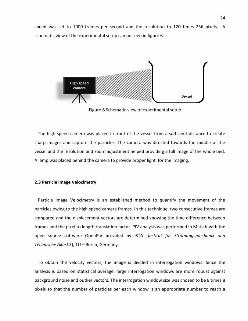
schematic view of the experimental setup can be seen in figure 6.

The high speed camera was placed in front of the vessel from a sufficient distance to create

sharp images and capture the particles. The camera was directed towards the middle of the

vessel and the resolution and zoom adjustment helped providing a full image of the whole bed.

A lamp was placed behind the camera to provide proper light for the imaging.

2.3 Particle Image Velocimetry

Particle Image Velocimetry is an established method to quantify the movement of the

particles owing to the high speed camera frames. In this technique, two consecutive frames are

compared and the displacement vectors are determined knowing the time difference between

frames and the pixel to length translation factor. PIV analysis was performed in Matlab with the

open source software OpenPIV provided by ISTA (Institut für Strömungsmechanik und

Technische Akustik), TU – Berlin, Germany.

To obtain the velocity vectors, the image is divided in interrogation windows. Since the

analysis is based on statistical average, large interrogation windows are more robust against

background noise and outlier vectors. The interrogation window size was chosen to be 8 times 8

pixels so that the number of particles per each window is an appropriate number to reach a

Figure 6 Schematic view of experimental setup.

25

proper averaged velocity field. The size should not be too large or too small since individual or

bulk displacements may be missed respectively. To control the size of the interrogation

windows and set the resolution of the two components of the velocity field, the spacing and

overlap: 8x8 pixels. A global and local filtering was applied in which the vectors which length is

larger than the mean flow plus 3 times its standard deviation are removed. Vectors that are

dissimilar from the close neighbors are removed and the missing values are interpolated from

the neighbor vector values.

2.4 Data post-processing

After the PIV is executed, velocity vectors are obtained as matrices containing the two

components of the velocity field. The velocity vector units are not in physical units. To translate

into [m/s], the time between two frames is required and the relation between meters and pixels

in the images, i.e. the image size and the number of pixels. A post-processing procedure in

Matlab calculates the average velocity profiles and the intensity of velocity fluctuations for each

case. The average intensity of fluctuations has been achieved by calculating the standard

deviation of the velocity field.

CHAPTER 3

NUMERICAL MODELLING

Fluent 14.5 (ANSYS Inc., US) was used to perform the simulations. The mesh was imported

from a previous case from Darelius et al. (2008). It was constructed in Gambit version 2.3.16

(ANSYS Inc., US) and the impeller geometry was based on an imported CAD drawing of the

original impeller.

The material’s properties have been defined to make it comparable to the experimental work;

particle density was set to glass density 2700 kg/m3 and viscosity of 10 kg/m.s to give it a solid

behavior. More particles were patched to reach approximately 500 cm3 and have more dense

regions in the system (total mass 1.48 kg) compared to the starting case. They were initially

patched at the bottom of the vessel, but since the simulation is starting from an already solved

case with particles suspended in the vessel, the increased value of the density increases the

particle mass, hence the possibility that they cluster at the bottom. This dense region at the

bottom involves more complicated phenomena and caused convergence problems; to solve

this, the regions that had volume fraction between 0.15 and 0.3 were patched using iso-value to

have a new value of 0.5, in this way the dense regions would be distributed in the interior of the

vessel.

3.1 Mesh and geometry

The sliding mesh approach is employed to tackle the rotation of the impeller blades: one part

of the geometry rotates with respect to the other one and the momentum fluxes across the

interface between the two sub-domains are matched in each time step. The two sub-domains

can be seen in figure 7.

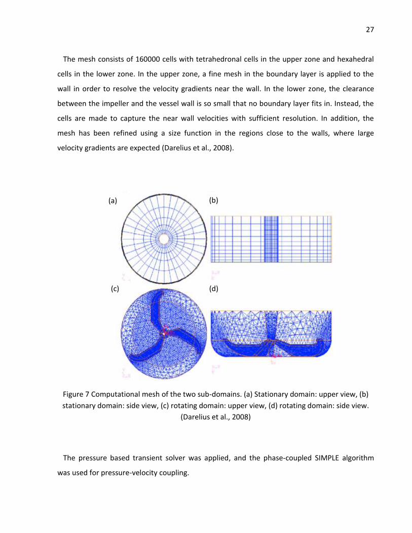
27

The mesh consists of 160000 cells with tetrahedronal cells in the upper zone and hexahedral

cells in the lower zone. In the upper zone, a fine mesh in the boundary layer is applied to the

wall in order to resolve the velocity gradients near the wall. In the lower zone, the clearance

between the impeller and the vessel wall is so small that no boundary layer fits in. Instead, the

cells are made to capture the near wall velocities with sufficient resolution. In addition, the

mesh has been refined using a size function in the regions close to the walls, where large

velocity gradients are expected (Darelius et al., 2008).

Figure 7 Computational mesh of the two sub-domains. (a) Stationary domain: upper view, (b)

stationary domain: side view, (c) rotating domain: upper view, (d) rotating domain: side view.

(Darelius et al., 2008)

The pressure based transient solver was applied, and the phase-coupled SIMPLE algorithm

was used for pressure-velocity coupling.

(a) (b)

(c) (d)

28

3.2 Frictional viscosity and solids pressure

Granular viscosity and granular bulk viscosity were solved using Syamlal et al. and Lun et al.,

respectively (see Section 1.2, eq 4 and eq 5). To account for frictional viscosity, the rheology

model has been applied using User Defined Functions (UDFs) (see Section 1.3). The model

switches to KTGF in the regions where the volume fraction goes under the frictional packing

limit, which was initially set to 0.55.

The formulation for pressure given by eq 14 has been included in the UDF file to account for

the pressure in the dense regions of the system. For this, the bed shape has been considered.

To simplify the determination of , a projected triangular shape was assumed for the bed

shape as it is shown in figure 8. The shape of the bed can be compared with a triangle if it would

be projected on a 2D plane. To obtain the column height, information on the position of cells

was used; for example, the height of the column over point A (see figure 8), would be

equivalent to the position of point B minus the position of point A, where point B will always fall

over the hypotenuse of the triangle and point A will be at any point inside the triangle.

Figure 8 Bed shape and projected triangle in a 2D plane.

Z

y

A

B

29

The slight deviation of the real bed shape from a triangle would lead to underestimation of

the column height in the upper part and an overestimation in the lower part; however, due to

the low values of volume fraction in these regions the error is considered to be negligible.

3.3 Boundary conditions

The gas phase is assumed to obey no slip boundary condition at the walls and on the impeller.

For the solid phase, partial slip condition has been applied using the relation in eq 15 that

provides the degree of partial slip at the boundaries of the system.

|

(15)

where, is the relative velocity of the solid phase at the wall and is the normal direction of

the wall. Thus, “b/a” gives the degree of partial slip with 0 corresponding to no slip and infinity

to full slip. The degree of partial-slip could be represented by the torque exerted on the

impeller, which characterizes the amount of energy transferred from the whole system to the

particles.

Due to the partial slip boundary conditions it was difficult to reach convergence; the under

relaxation factor were gradually increased until obtaining 0.05 for pressure and 0.2 for

momentum.

CHAPTER 4

RESULTS AND DISCUSSION

The results obtained by the methods described in the previous chapters are presented and

discussed below. This chapter includes a discussion on the velocity profiles obtained

experimentally using PIV analysis, a description on visual observations of the system, a

comparison of the experimental and simulation results, and finally a discussion on the accuracy

of the numerical model.

Velocity profiles have been obtained for different positions. In order to obtain instantaneous

velocity fields with angular resolution instead of averaged fields, the 120° span between two

consecutive blades was divided into 4 groups with respect to the angular distance to the blades

to study the flow behavior and velocity profiles with respect to impeller position. The location of

the different groups is shown in figure 9.

Figure 9 Angle span between blades.

31

The impeller speed is chosen to be 500 rpm. 2000 frames have been taken in two seconds

which gives over 80 frames per group per pass. The first blade was marked in the equipment

and it was visually identified during the PIV analysis to determine which frames corresponds to

which group. Axial and tangential velocity profiles have been quantified by PIV whereas due to

experimental limitations there is no access to the radial velocities. The clockwise direction is

assumed as positive direction of the tangential velocities since the impeller rotates clockwise.

The upward direction is assumed as axially positive. The region below 2cm height is considered

unreliable due to limited visibility and the curvature of the vessel.

4.1 Visual observations

A periodical phenomenon with the periodicity of one revolution is observed. The first blade

“breaks” the bed and pushes the largest amount of particles upward showing the lowest values

for axial velocity; when the next blade passes, the amount of particles in the neighboring region

is significantly lower having a greater impact in the axial component of the velocity. Finally,

some particles fill up the area neighboring the blade and the axial velocity reaches an

intermediate value.

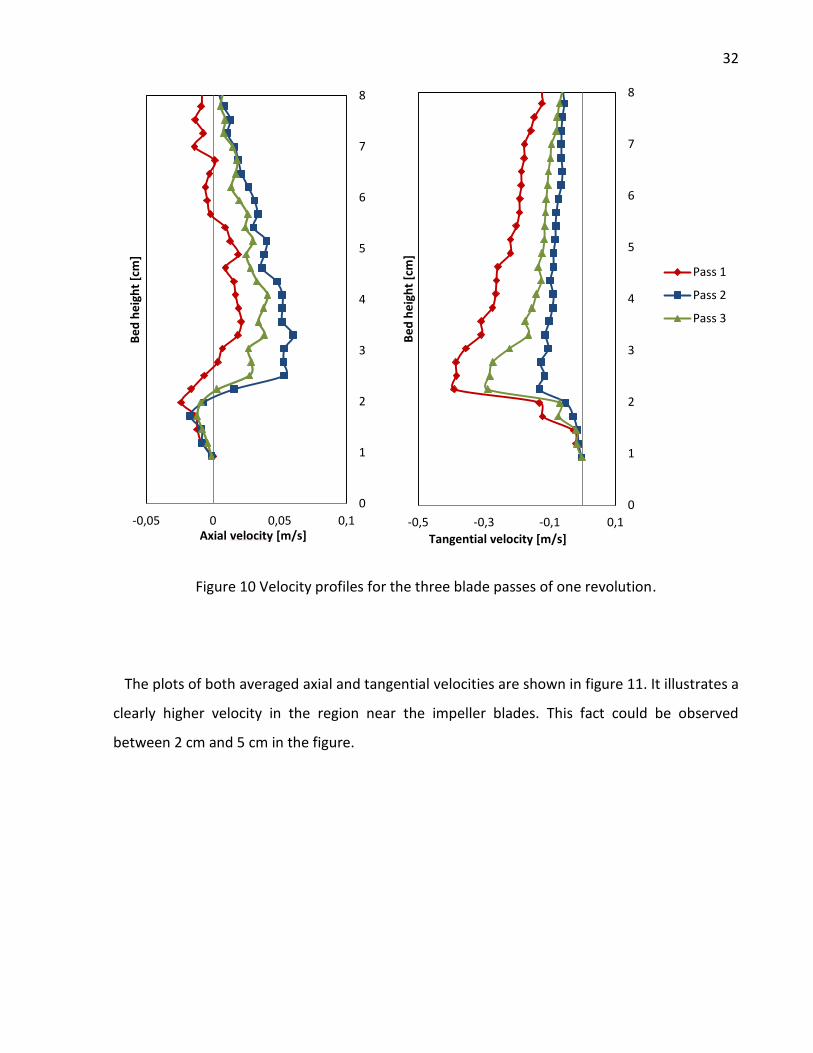
4.2 Velocity profiles (PIV)

Accordingly to the visual observations, figure 10 shows different axial velocity profiles for each

of the 3 passes of one revolution from the images obtained with the high speed camera.

32

Figure 10 Velocity profiles for the three blade passes of one revolution.

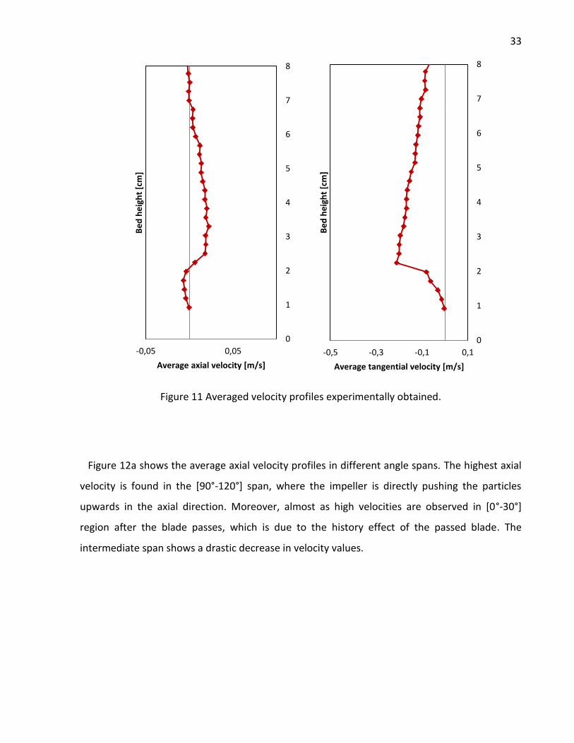
The plots of both averaged axial and tangential velocities are shown in figure 11. It illustrates a

clearly higher velocity in the region near the impeller blades. This fact could be observed

between 2 cm and 5 cm in the figure.

0

1

2

3

4

5

6

7

8

-0,05 0 0,05 0,1

Be

d h

eig

ht

[cm

]

Axial velocity [m/s]

0

1

2

3

4

5

6

7

8

-0,5 -0,3 -0,1 0,1

Be

d h

eig

ht

[cm

]

Tangential velocity [m/s]

Pass 1

Pass 2

Pass 3

33

Figure 11 Averaged velocity profiles experimentally obtained.

Figure 12a shows the average axial velocity profiles in different angle spans. The highest axial

velocity is found in the [90°-120°] span, where the impeller is directly pushing the particles

upwards in the axial direction. Moreover, almost as high velocities are observed in [0°-30°]

region after the blade passes, which is due to the history effect of the passed blade. The

intermediate span shows a drastic decrease in velocity values.

0

1

2

3

4

5

6

7

8

-0,05 0,05

Be

d h

eig

ht

[cm

]

Average axial velocity [m/s]

0

1

2

3

4

5

6

7

8

-0,5 -0,3 -0,1 0,1

Be

d h

eig

ht

[cm

]

Average tangential velocity [m/s]

34

Figure 12 Axial velocity profiles with respect to impeller position: (a) from experimental, (b)

from simulation.

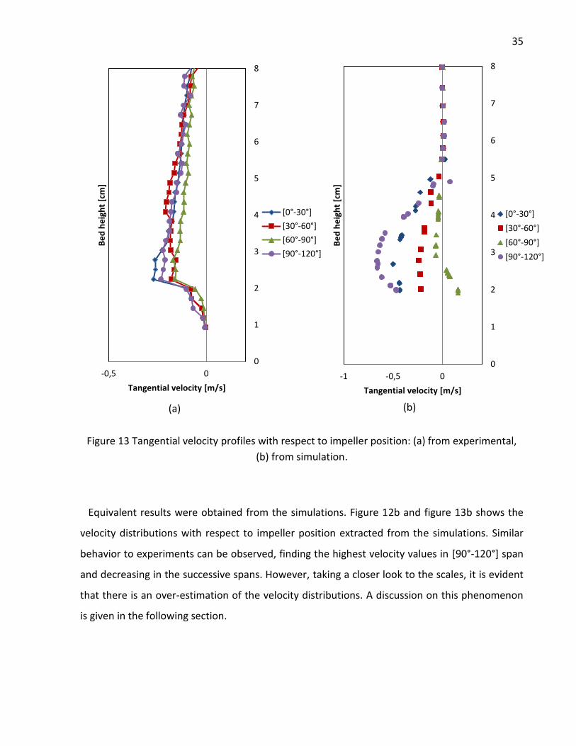
Similar to the results for the axial velocity the highest values for tangential velocity are found

in [90°-120°] span, as shown in figure 13a, due to the pushing effect of the impeller blade. [0°-

30°] shows almost as high velocities as [90°-120°] due to the history effect from the passed

blade and the values decrease in the subsequent spans.

0

1

2

3

4

5

6

7

8

-0,5 0 0,5 1

Be

d h

eig

ht

[cm

]

Axial velocity [m/s]

[0°-30°]

[30°-60°]

[60°-90°]

[90°-120°]

0

1

2

3

4

5

6

7

8

-0,05 0 0,05

Be

d h

eig

ht

[cm

]

Axial velocity [m/s]

[0°-30°]

[30°-60°]

[60°-90°]

[90°-120°]

(a) (b)

35

Figure 13 Tangential velocity profiles with respect to impeller position: (a) from experimental,

(b) from simulation.

Equivalent results were obtained from the simulations. Figure 12b and figure 13b shows the

velocity distributions with respect to impeller position extracted from the simulations. Similar

behavior to experiments can be observed, finding the highest velocity values in [90°-120°] span

and decreasing in the successive spans. However, taking a closer look to the scales, it is evident

that there is an over-estimation of the velocity distributions. A discussion on this phenomenon

is given in the following section.

(a)

0

1

2

3

4

5

6

7

8

-1 -0,5 0

Be

d h

eig

ht

[cm

]

Tangential velocity [m/s]

[0°-30°]

[30°-60°]

[60°-90°]

[90°-120°]

0

1

2

3

4

5

6

7

8

-0,5 0

Be

d h

eig

ht

[cm

]

Tangential velocity [m/s]

[0°-30°]

[30°-60°]

[60°-90°]

[90°-120°]

(b)

36

4.3 Numerical model

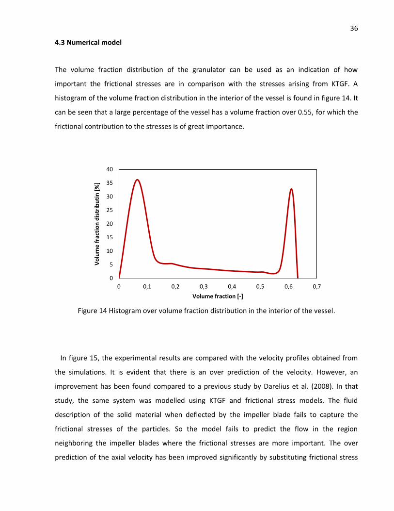
The volume fraction distribution of the granulator can be used as an indication of how

important the frictional stresses are in comparison with the stresses arising from KTGF. A

histogram of the volume fraction distribution in the interior of the vessel is found in figure 14. It

can be seen that a large percentage of the vessel has a volume fraction over 0.55, for which the

frictional contribution to the stresses is of great importance.

Figure 14 Histogram over volume fraction distribution in the interior of the vessel.

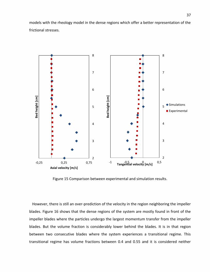
In figure 15, the experimental results are compared with the velocity profiles obtained from

the simulations. It is evident that there is an over prediction of the velocity. However, an

improvement has been found compared to a previous study by Darelius et al. (2008). In that

study, the same system was modelled using KTGF and frictional stress models. The fluid

description of the solid material when deflected by the impeller blade fails to capture the

frictional stresses of the particles. So the model fails to predict the flow in the region

neighboring the impeller blades where the frictional stresses are more important. The over

prediction of the axial velocity has been improved significantly by substituting frictional stress

0

5

10

15

20

25

30

35

40

0 0,1 0,2 0,3 0,4 0,5 0,6 0,7

Vo

lum

e f

ract

ion

dis

trib

uti

n [

%]

Volume fraction [-]

37

models with the rheology model in the dense regions which offer a better representation of the

frictional stresses.

Figure 15 Comparison between experimental and simulation results.

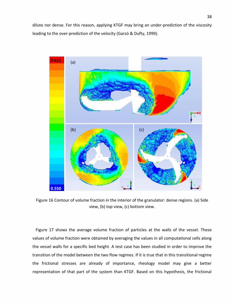
However, there is still an over-prediction of the velocity in the region neighboring the impeller

blades. Figure 16 shows that the dense regions of the system are mostly found in front of the

impeller blades where the particles undergo the largest momentum transfer from the impeller

blades. But the volume fraction is considerably lower behind the blades. It is in that region

between two consecutive blades where the system experiences a transitional regime. This

transitional regime has volume fractions between 0.4 and 0.55 and it is considered neither

2

3

4

5

6

7

8

-0,25 0,25 0,75

Be

d h

eig

ht

[cm

]

Axial velocity [m/s]

2

3

4

5

6

7

8

-1 -0,5 0 0,5

Be

d h

eig

ht

[cm

]

Tangential velocity [m/s]

Simulations

Experimental

38

dilute nor dense. For this reason, applying KTGF may bring an under-prediction of the viscosity

leading to the over-prediction of the velocity (Garzó & Dufty, 1999).

Figure 16 Contour of volume fraction in the interior of the granulator: dense regions. (a) Side

view, (b) top view, (c) bottom view.

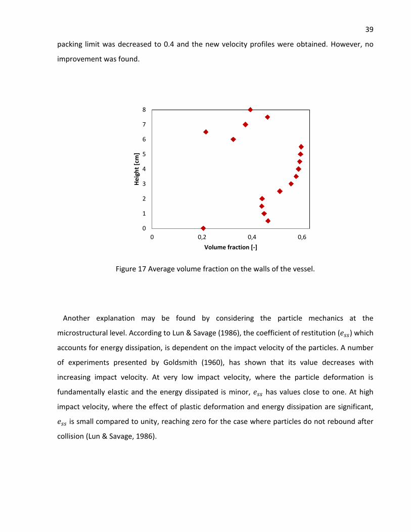
Figure 17 shows the average volume fraction of particles at the walls of the vessel. These

values of volume fraction were obtained by averaging the values in all computational cells along

the vessel walls for a specific bed height. A test case has been studied in order to improve the

transition of the model between the two flow regimes. If it is true that in this transitional regime

the frictional stresses are already of importance, rheology model may give a better

representation of that part of the system than KTGF. Based on this hypothesis, the frictional

0.621

0.550

(a)

(b) (c)

39

packing limit was decreased to 0.4 and the new velocity profiles were obtained. However, no

improvement was found.

Figure 17 Average volume fraction on the walls of the vessel.

Another explanation may be found by considering the particle mechanics at the

microstructural level. According to Lun & Savage (1986), the coefficient of restitution ( ) which

accounts for energy dissipation, is dependent on the impact velocity of the particles. A number

of experiments presented by Goldsmith (1960), has shown that its value decreases with

increasing impact velocity. At very low impact velocity, where the particle deformation is

fundamentally elastic and the energy dissipated is minor, has values close to one. At high

impact velocity, where the effect of plastic deformation and energy dissipation are significant,

is small compared to unity, reaching zero for the case where particles do not rebound after

collision (Lun & Savage, 1986).

0

1

2

3

4

5

6

7

8

0 0,2 0,4 0,6

He

igh

t [c

m]

Volume fraction [-]

40

Several cases were carried out for different values of coefficient of restitution, which values

were kept low based on the fact that the particles will have high impact velocities under a high

shear at the given impeller speed. However, no significant variations were observed.

For particulate systems under high shear, the particles will collide with different impact

velocities depending on the rate of shear, and the coefficient of restitution will vary (Lun &

Savage, 1986). This variability on energy dissipation is not accounted for in the simulations

where the coefficient of restitution has a constant value. However, it is possible to reduce the

error and estimate an approximate value by taking the ratio of the mean separation distance of

the particles to the mean time interval between successive collisions (Lun & Savage, 1986).

Furthermore, this over prediction of the velocity could as well be due to the tangential partial

slip condition at the impeller surface. As stated in Chapter 3, the degree of slip is dependent

upon the relative velocity of the solid phase at the wall. Capturing the partial slip condition in

the walls of the three-bladed impeller is not trivial. The relative velocity becomes a relative

velocity between the moving particles and the rotating impeller, so that the degree of slip will

also be a function of the shape, radius and speed of the impeller.

CONCLUSIONS

It can be concluded that applying KTGF and rheology model in Eulerian-Eulerian framework is

a good strategy for modeling multi-regime granular flows. The model smoothly switches

between KTGF in the dilute regions of the system and rheology model in the dense regions

based on a Inertial Number. Besides, the replacement of Schaeffer’s extension of KTGF for

rheology model has shown an improvement on the prediction of velocity compared to previous

studies.

Comparing the experimental results with the simulations, an over-prediction of axial a

tangential velocities were found. No improvement was found from applying rheology model to

the transitional regions between dilute and dense instead of applying KTGF. Different values for

low coefficient of restitution were tried and no significant variations were observed; a constant

assumption of constant coefficient of restitution could miss the variability of energy dissipation

due to the different impact velocities of the particles. Capturing the partial slip condition at the

walls of the three-bladed impeller is difficult to achieve since it will depends on rotational speed

and geometric configuration of the impeller.

Further work should be performed to adapt the existing models or find a new model that

provides a better description of the transitional region. Perform mesh refinement in regions

with high gradients and investigate the particle-impeller interaction.

REFERENCES

Abrahamsson, P. J., Björn, I. N., & Rasmuson, A. (2013). Parameter study of a kinetic-frictional continuum model of a disk impeller high-shear granulator. Powder Technology, 238, 20–26. doi:10.1016/j.powtec.2012.07.015

Baer, M. R., & Nunziato, J. W. (1986). A two-phase mixture theory for the deflagration-to-detonation transition (ddt) in reactive granular materials. International Journal of Multiphase Flow, 12(6), 861–889. doi:10.1016/0301-9322(86)90033-9

Bagnold, R. A. (1954). Experiments on a gravity-free dispersion of large solid spheres in a Newtonian fluid under shear. Proceedings of the Royal Society of London, 225, 49–63.

Da Cruz, F., Emam, S., Prochnow, M., Roux, J.-N., & Chevoir, F. (2005). Rheophysics of dense granular materials : Discrete simulation of plane shear flows. Phys. Rev.

Darelius, A., Rasmuson, A., van Wachem, B., Niklasson Björn, I., & Folestad, S. (2008). CFD simulation of the high shear mixing process using kinetic theory of granular flow and frictional stress models. Chemical Engineering Science, 63(8), 2188–2197. doi:10.1016/j.ces.2008.01.018

Darelius, A., Remmelgas, J., Rasmuson, A., van Wachem, B., & Björn, I. N. (2010). Fluid dynamics simulation of the high shear mixing process. Chemical Engineering Journal, 164(2-3), 418–424. doi:10.1016/j.cej.2009.12.020

Garzó, V., & Dufty, J. W. (1999). Dense fluid transport for inelastic hard spheres. Physical Review. E, Statistical Physics, Plasmas, Fluids, and Related Interdisciplinary Topics, 59(5 Pt B), 5895–911. Retrieved from http://www.ncbi.nlm.nih.gov/pubmed/11969571

Goldsmith, W. (1960). Impact: The theory and physical behavior of colliding solids. Arnold.

Hatano, T. (2007). Rheology of a dense granular material. Journal of Physics: Conference Series, 89, 012015. doi:10.1088/1742-6596/89/1/012015

Iveson, S. M., Litster, J. D., Hapgood, K., & Ennis, B. J. (2001). Nucleation, growth and breakage phenomena in agitated wet granulation processes: a review. Powder Technology, 117(1-2), 3–39. doi:10.1016/S0032-5910(01)00313-8

Jackson, R. (1997). Locally Averaged Equations of Motion for a Mixture of Identical Spherical Particles and a Newtonian Fluid. Chem. Eng. Sci., (52), 2457.

Jaeger, H., Nagel, S., & Behringer, R. (1996). Granular solids, liquids, and gases. Reviews of Modern Physics, 68(4), 1259–1273. doi:10.1103/RevModPhys.68.1259

43

Jenkins, J.J. and Savage, S. B. (1983). A theory for the rapid flow of identical smooth nearly elastic spherical particles. Journal of Fluid Mechanics, 130(187).

Johnson, P. C., & Jackson, R. (1987). Frictional–collisional constitutive relations for granular materials, with application to plane shearing. Journal of Fluid Mechanics, 176, 66–93. doi:10.1017/S0022112087000570

Jop, P., Forterre, Y., & Pouliquen, O. (2005). Crucial role of sidewalls in granular surface flows: consequences for the rheology. Journal of Fluid Mechanics, 541(-1), 167. doi:10.1017/S0022112005005987

Jop, P., Forterre, Y., & Pouliquen, O. (2006). A constitutive law for dense granular flows. Nature, 441(7094), 727–30. doi:10.1038/nature04801

Josserand, C., Lagrée, P.-Y., & Lhuillier, D. (2006). Granular pressure and the thickness of a layer jamming on a rough incline. Europhysics Letters (EPL), 73(3), 363–369. doi:10.1209/epl/i2005-10398-1

Khalilitehrani, M., Abrahamsson, P. J., & Rasmuson, A. (2013). The rheology of dense granular flows in a disc impeller high shear granulator. Powder Technology, 249, 309–315. doi:10.1016/j.powtec.2013.08.033

Khalilitehrani, M., Abrahamsson, P. J., & Rasmuson, A. (2014). Modeling dilute and dense granular flows in a high shear granulator. Powder Technology, 263, 45–49. doi:10.1016/j.powtec.2014.04.088

Litster, J. D. (2003). Scaleup of wet granulation processes: science not art. Powder Technology, 130(1-3), 35–40. doi:10.1016/S0032-5910(02)00222-X

Lun, C. K. K., & Savage, S. B. (1986). The Effects of an Impact Velocity Dependent Coefficient of Restitution on Stresses Developed by Sheared Granular Materials. Acta Mech., 44.

Lun, C.K.K, Savage, S.B. and Chepurning, N. (1984). Kinetic theories for granular flow: Inelastic particles in Couette flow and single inelastic particles in a general flow field. Journal of Fluid Mechanics, 140(223).

Midi, G. D. R. (2004). On dense granular flows. The European Physical Journal. E, Soft Matter, 14(4), 341–65. doi:10.1140/epje/i2003-10153-0

Parikh, D. M. (Ed.). (1997). Handbook of Pharmaceutical Granulation Technology. New York: Marcel Dekker.

Pouliquen, O. (1999). Scaling laws in granular flows down rough inclined planes. Physics of Fluids, 11(3), 542–548. doi:10.1063/1.869928

44

S.A. Ogawa, A. Umemuta, N. O. (1980). On the equations for fluidized granular materials. Journal of Applied Mathematics and Physic, 31(483).

Savage, S. B. and Jeffrey, D. J. (1981). The stress tensor in a granular flow at high shear rates. Journal of Fluid Mechanics, 110(457).

Schaeffer, D. G. (1987). Instability in the evolution equations describing incompressible granular flow. Journal of Differential Equations, 66(1), 19–50. doi:10.1016/0022-0396(87)90038-6

Syamlal, M., Rogers, W., & O’Brien, T. . (1993). MFIX Documentation: Volume1, Theory Guide (pp. 2353–2373). Springerfield.

Van Wachem, B., Schouten, J. C., van den Bleek, C. M., Krishna, R., & Sinclair, J. L. (2001). Comparative analysis of CFD models of dense gas–solid systems. AIChE Journal, 47(5), 1035–1051. doi:10.1002/aic.690470510