Coupling Basin- and Site-Scale Inverse Models o the Espanola Aquifer by Elizabeth H. Keating 1, Velimir V. Vesselinov 1, Edward Kwicklis 1, and Zhiming Lu 1

Abstract/ Large-scale models are frequently used to estimate fluxes to small-scale models. The uncertainty associated with

these flux estimates, however, is rarely addressed. We present a case study from the Espanola Basin, northern New Mexico, where we use a basin-scale model coupled with a high-resolution, nested site-scale model. Both models are three-dimensional and are analyzed by codes FEHM and PEST. Using constrained nonlinear optimization, we exam­ine the effect of parameter uncertainty in the basin-scale model on the nonlinear confidence limits of predicted fluxes to the site-scale model. We find that some of the fluxes are very well constrained, while for others there is fairly large uncertainty. Site-scale transport simulation results, however, are relatively insensitive to the estimated uncertainty in the fluxes. We also compare parameter estimates obtained by the basin- and site-scale inverse models. Differences in the model grid resolution (scale of parameter estimation) result in differing delineation of hydrostratigraphic units, so the two models produce different estimates for some units. The effect is similar to the observed scale effect in medium properties owing to differences in tested volume. More important, estimation uncertainty of model parameters is quite different at the two scales. Overall, the basin inverse model resulted in significantly lower estimates of uncertainty, because of the larger calibration dataset available. This suggests that the basin-scale model contributes not only important boundary condition information but also improved parameter identification for some units. Our results demonstrate that caution is warranted when applying parameter estimates inferred from a large-scale model to small­scale simulations, and vice versa.

Introduction The most straightforward method to obtain fine grid

resolution in the region of interest and maintain consistency with a larger-scale flow field is to refine the large-scale model grid selectively (Kernodle and Thorn 1995; Tiede­man et al. 1998; Meier 1999; Keating et al. 2000a; Vesseli­nov and Neuman, 2001). This method, however, may not produce sufficient resolution in the area of interest without significantly increasing the total number of grid elements; this is a particularly severe problem with finite-difference methods. Amore complex approach is to build nested mod­els (telescopic mesh refinement) (Ward et al. 1987; Keating and Bahr 1998; Leake et al. 1998; Walker and Gylling 1998; Hunt et al. 2001; Zyvoloski et al. 2002). Nested mod­els can be coupled either through specified-flux or speci­fied-head boundary conditions; specified-flux conditions

1Earth and Environmental Sciences Division, Los Alamos National Laboratory, Los Alamos, NM 87545; ekeating@lanl.gov, vvv@lanl.gov, kwicklis@lanl.gov, zhiming@lanl.gov

have the advantage of conserving mass in the coupled model system. This is especially important if the site-scale model is used to predict the effect of pumping (Giudici et al. 2001). For transient simulations, it may be necessary to specify transient flux boundary conditions (Anderson and Woessner 1992).

In this paper, we discuss parameter uncertainty in site­scale and basin-scale models and investigate two aspects of coupling nested models. The first is the potential differ­ences between estimates of parameters and parameter uncertainty provided by inverse modeling at the two scales. Adjusting parameters within the site-scale model inde­pendently of basin-scale calibration is common (Hunt et al. 2001; Zyvoloski et al. 2002). Calibration of the two mod­els simultaneously, even with weak coupling, has not been reported in the literature. The second aspect is related to evaluation of sources of uncertainty in the site-scale model. There will be a number of possible sources of uncertainty for any prediction made using the site-scale model. We have explored, for example, the influence of parameter uncertainty on ground water flow directions (Keating et al. 2000b). In this paper, we apply a method for quantifying

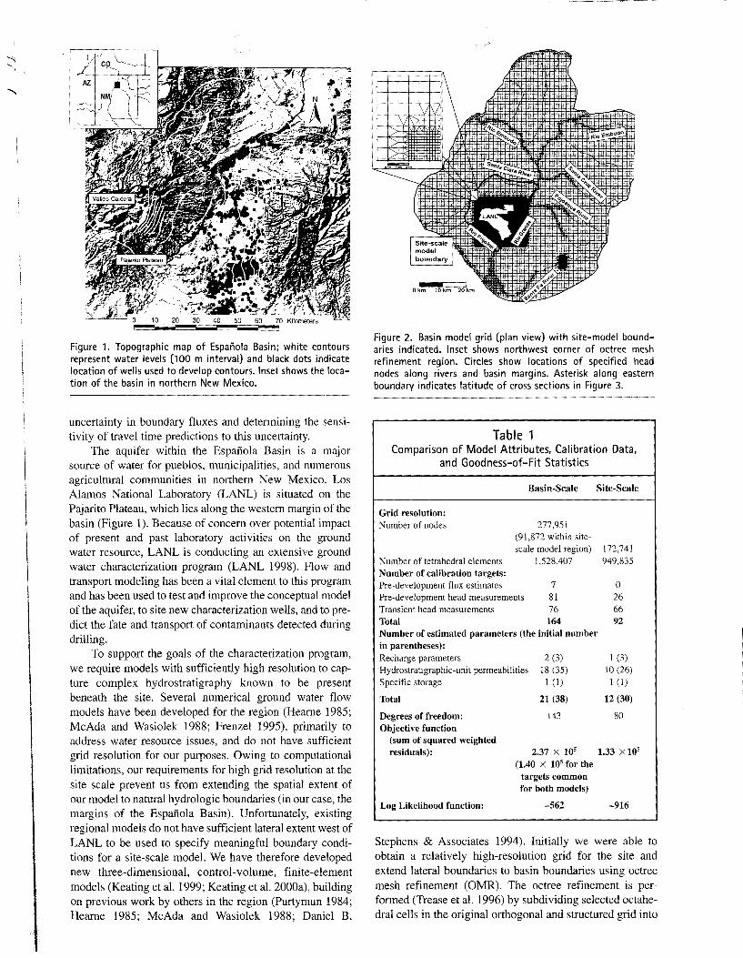
Figure 1. Topographic map of Espanola Basin; white contours represent water levels (100 m interval) and black dots indicate location of wells used to develop contours. Inset shows the loca­tion of the basin in northern New Mexico.

uncertainty in boundary fluxes and determining the sensi­tivity of travel time predictions to this uncertainty.

The aquifer within the Espanola Basin is a major source of water for pueblos, municipalities, and numerous agricultural communities in northern New Mexico. Los Alamos National Laboratory (LANL) is situated on the Pajarito Plateau, which lies along the western margin of the basin (Figure 1). Because of concern over potential impact of present and past laboratory activities on the ground water resource, LANL is conducting an extensive ground water characterization program (LANL 1998). Flow and transport modeling has been a vital element to this program and has been used to test and improve the conceptual model of the aquifer, to site new characterization wells, and to pre­dict the fate and transport of contaminants detected during drilling.

To support the goals of the characterization program, we require models with sufficiently high resolution to cap­ture complex hydrostratigraphy known to be present beneath the site. Several numerical ground water flow models have been developed for the region (Hearne 1985; McAda and Wasiolek 1988; Frenzel 1995), primarily to address water resource issues, and do not have sufficient grid resolution for our purposes. Owing to computational limitations, our requirements for high grid resolution at the site scale prevent us from extending the spatial extent of our model to natural hydrologic boundaries (in our case, the margins of the Espanola Basin). Unfortunately, existing regional models do not have sufficient lateral extent west of LANL to be used to specify meaningful boundary condi­tions for a site-scale model. We have therefore developed new three-dimensional, control-volume, finite-element models (Keating et al. 1999; Keating et al. 2000a), building on previous work by others in the region (Purtymun 1984; Hearne 1985; McAda and Wasiolek 1988; Daniel B.

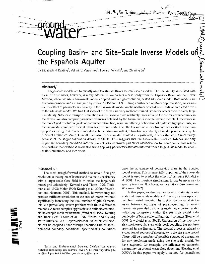
Figure 2. Basin model grid (plan view) with site-model bound­aries indicated. Inset shows northwest corner of octree mesh refinement region. Circles show locations of specified head nodes along rivers and basin margins. Asterisk along eastern boundary indicates latitude of cross sections in Figure 3.

Table 1 Comparison of Model Attributes, Calibration Data,

and Goodness-of-Fit Statistics

Basin-Scale Site-Scale

Grid resolution: Number of nodes 277,951

(91,872 within site-scale model region) 172,741

Number of tetrahedral elements I ,528,407 949,835 Number of calibration targets: Pre-development flux estimates 7 0 Pre-development head measurements 81 26 Transient head measurements 76 66 Total 164 92 Number of estimated parameters (the initial number in parentheses): Recharge parameters 2 (3) I (3) Hydrostratigraphic-unit permeabilities 18 (35) 10 (26) Specific storage I (I) I (I)

Total 21 (38) 12 (30)

Degrees of freedom: 143 80 Objective function

(sum of squared weighted residuals): 2.37 X 105 1.33 X 105

(1.40 X 105 for the targets common for both models)

Log Likelihood function: -562 -916

Stephens & Associates 1994). Initially we were able to obtain a relatively high-resolution grid for the site and extend lateral boundaries to basin boundaries using octree mesh refinement (OMR). The octree refinement is per­formed (Trease et al. 1996) by subdividing selected octahe­dral cells in the original orthogonal and structured grid into

2500

2000

g 1500 r::: 0 +" co 1000 > Q)

jjj

500

0

1900

1800

~ .s 6 ~ 1700 ~ .Ill w

1600

IX

IX

IX

IX

IX

IX

IX 150

P5ooo

1900

1800

.s 6 ~ 1700 ~

.Ill w

1600

r

IS

1\ 15~~000

1\ 1\

1\ 1\

1\ 1\ IX IX 1\ 1\

1\ 1\ 1\ IX IY 1\ 1\

1\ 1\ 1\ IX 1\

1\ 1\ 1\ IX 1\

1\ 1\ 1\ IX 1\ 20000

1'\1

II lXIXI

R

IX 1\ 1\ 1/ IX

1\ IX 1\ 1/ IX IX 1/ 20000

X{m) a

Basin-scale model

1\ 1\ 1/ IX 1\ 1\ IX

IX 1\ 1\ IX IX 1\ 1\ IX IX 1\ 1\

IX 1\ 1\ IX 1\ 1\ IX 1\ 1\ 1/ IX

IX 1\ 1\ IX 1\ IX 1\ 1\ IX

IX 1\ 1\ IX IX 1\ IX 1\ IX 1\

IX 1\ 1\ IX IX 1\ 1\ IX 1\ IX 1\ b 25000 30000

X {m)

Site-scale model

1\ 1/ 1\ II 1\

I~ 1\ I,\ 1/ IX 1\ IX 1\ 1\ 1/ c 25000 30000

X{m)

Figure 3. Cross-sectional views of basin- and site-scale grids: (a) basin grid; box shows location of views in (b) and (c); (b) zoomed basin grid; (c) zoomed site grid. Black circles in (b) and (c) show nodes identified as basalt.

eight octahedral cells. The refined "r~~odel provided very good control on mass flux through the system and reason­ably detailed site-scale transport calculations; however, it ultimately failed to provide sufficient vertical resolution at the site scale to capture significant hydrostratigraphic fea­tures with adequate resolution. To achieve the higher reso­lution, we are coupling two models: this OMR basin-scale model with relatively coarse vertical resolution (50 m) to a site-scale model with an increased vertical resolution (12.5 m). Our modeling approach uses the FEHM (finite element heat and mass transfer) code (Zyvoloski et al. 1997) to sim­ulate flow and transport and the PEST code (Doherty, 2000) to estimate parameters and evaluate uncertainty of model parameters and predictions (Keating et al. 2000a; Keating and Vesselinov 2001; Vesselinov et al. 2001).

Hydrologic Setting The Espanola Basin (Figure 1) is in northern New

Mexico. It is one of a series of basins located within the Rio Grande Rift zone, a tectonic feature that extends from northern Colorado to the south into Mexico. Elevations within the basin range from more than 3800 m along peaks in the surrounding mountain ranges to -1700 m at the Rio Grande near the basin outlet. Vegetation is predominately ponderosa pine forest at higher elevations and pinon pine/juniper at lower elevations (Spiegel and Baldwin 1963, p. 17).

The aquifer comprises predominately Santa Fe Group rocks, which are poorly consolidated basin-fill sediments reaching more than 3000 m in thickness near the basin axis (Cordell 1979). Ground water also occurs in older crys­talline rocks along the eastern and northern basin margin and in younger volcanic lavas and volcaniclastic sedimen­tary rocks in the vicinity of the Pajarito Plateau to the west (Purtymun and Johansen 1974; Coon and Kelly 1984; Daniel B. Stephens & Associates 1994).

The vadose zone is -0 to 60 m thick in most parts of the basin, much thicker on the Pajarito Plateau (up to 350 m) where perched aquifers also exist. Contours of water level data (Purtymun et al. 1995; U.S. Geological Survey 1997) indicate that hydraulic gradients are generally toward the Rio Grande (Figure 1). Water enters the aquifer as inter­flow from basins to the north and as recharge. Water leaves the aquifer at numerous water supply and irrigation wells, as interflow to basins to the south, and to the Rio Chama, the Rio Grande and the lower reaches of its tributaries. Median monthly flow, calculated using USGS average monthly flow data for the last 80 years, is 26.0 m3/sec along the Rio Grande (at Otowi Bridge) and 10.0 m3/sec along the Rio Chama (at Chamita) (USGS 2000). Because of recent exploitation of ground water resources in the basin, some reaches of these rivers and their tributaries, which were once ground water discharge zones, may now be recharging the aquifer.

The climate is semiarid; annual total precipitation ranges from 18 to 86 em/year. Precipitation increases with elevation (Spiegel and Baldwin 1963). Recharge is thought to occur primarily in the higher elevations-estimates based on water budget and chloride mass-balance methods

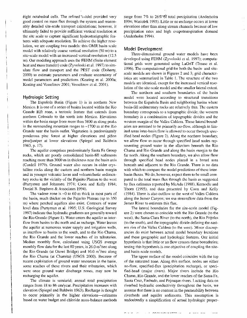
range from 7% to 26o/o'"~I total precipitation (Anderholm 1994; Wasiolek 1995). Little or no recharge occurs at lower elevations other than along stream channels because of low precipitation rates and high evapotranspiration demand (Anderholm 1994).

Model Development Three-dimensional ground water models have been

developed using FEHM (Zyvoloski et al. 1997); computa­tional grids were generated using LaGriT (Trease et al. 1996). The computational grid for both the basin- and site­scale models are shown in Figures 2 and 3; grid character­istics are summarized in Table 1. The structure of the two models are identical, except for the increased vertical reso­lution of the site-scale model and the smaller lateral extent.

The northern and southern boundaries of the basin model were located according to structural transitions between the Espanola Basin and neighboring basins where basin-fill sedimentary rocks are relatively thin. The eastern boundary corresponds to a topographic divide; the western boundary is a combination of topographic divides and the western margin of the Valles Caldera. These lateral bound­aries are assumed to be primarily no-flow, although in lim­ited areas inter-basin flow is allowed to occur through spec­ified head nodes (Figure 2). Along the northern boundary, we allow flow to occur through specified head nodes rep­resenting ground water in the alluvium beneath the Rio Chama and Rio Grande and along the basin margin to the far north. Along the southern boundary, we also allow flow through specified head nodes placed in a broad area beneath and adjacent to the Rio Grande. There is no data with which to compare the model predictions of these inter­basin fluxes. We do, however, expect them to be small com­pared to the total mass flux through the basin as suggested by flux estimates reported by McAda (1988), Kernodle and Thorn (1995), and data presented by Coon and Kelly (1984). There is also outflow to the west of Valles Caldera along the Jemez Canyon; we use streamflow data from the Jemez River to estimate this flux.

The lateral boundaries for the site-scale model (Fig­ure 2) were chosen to coincide with the Rio Grande (to the west), the Santa Clara River (to the north), the Rio Frijoles (to the south), and the topographic divide defining the east­ern rim of the Valles Caldera (to the west). Minor discrep­ancies do exist between actual model boundary locations and these geographic and hydrologic features. Our initial hypothesis is that little or no flow crosses these boundaries; testing this hypothesis is one objective of coupling the site­and basin-scale models.

The upper surface of the model coincides with the top of the saturated zone. Along this surface, nodes are either no-flow, specified-flux (precipitation recharge), or speci­fied-head (major rivers). Major rivers include the Rio Chama, Rio Grande, and the lower reaches of the Santa Fe, Santa Cruz, Embudo, and Pojoaque rivers. Lacking data on riverbed hydraulic conductivity throughout the basin, we assume that there is no contrast in the permeability between riverbeds and aquifer sediments. This assumption is undoubtedly a simplification of actual hydrologic proper-

,·~or

ties. By evaluating the model calibration and simulated river/aquifer fluxes (described later) we will test the impact of this simplifying assumption.

In our study, it is important to estimate not only the total amount but also the spatial distribution of ground water recharge from precipitation within the basin with cor­responding estimates of uncertainty. However, this requires that our recharge model can be parameterized and the respective parameters can be included in the inverse process. Although actual spatial and temporal patterns of recharge in the basin are undoubtedly complex, we use a very simple model that takes advantage of the strong ele­vation dependence of precipitation in the basin. We also assume recharge is constant in time. We define ground water recharge (R) over the model domain as follows:

R(x,y) =a ~(x,y)·P [Z(x,y)] (1)

{

1 Z(x,y) > Zmax

~(x,y) = zi::~~~~:' Zmin < Z(x,y) < Zmax (2)

0 Z(x,y) < Zmin

where P is precipitation, Z is ground-surface elevation defined from the digital elevation model of the region, ~ is a dimensionless weight function, which is characterized by parameters zmin and zmax' and a is the fraction of precipi­tation that becomes recharge above Zmax· Note that Zmin defines the elevation below which no recharge occurs, and above elevation Zmax the recharge is equal to a P. The total recharge flux Q over the model domain Q is defined as

Q = If Rdxdy = a If ~Pdxdy = aP' (Zmin,Zmax) (3) Q Q

where P' is a function of Zmin and Zmax only. We assume P(Z) is a simple linear model with fixed regression param­eters, which we derive using annual precipitation data for the region (Spiegel and Baldwin 1963; Bowen 1992). Thus, there are four unknowns to be estimated (Q, a, zmin' and Zmax) coupled through Equation 3. For example, to calcu­late Q we need to estimate a, Zmin' and Zmax· For our inverse models, we found it to be more computationally efficient to include Q, zmin' and zmax in the estimation process, and compute a as

(4)

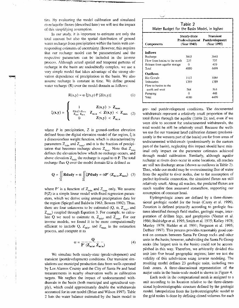
We simulate both steady-state (predevelopment) and transient (postdevelopment) conditions. Our transient sim­ulations use municipal production data from wells operated by Los Alamos County and the City of Santa Fe and head measurements in nearby observation wells as calibration targets. We neglect the impact of undocumented with­drawals in the basin (both municipal and agricultural sup­ply), which could approximately double the withdrawals accounted for in our model (Brian and Wilson 1997). Table 2 lists the -water balance estimated by the basin model in

Table 2 Water Budget for the Basin Model, in kg/sec

Steady-State Transient Predevelopment Postdevelopment

Components (Year 1945) (Year 1995)

Inflows Recharge 3845 3845 Flow from basins to the north 235 235 Release from aquifer storage 0 419 Total 4080 4499

Outflows Rio Grande 1112 1084 Tributaries 1389 1389 Flow to basins to the

south and west 564 564 Pumping 0 448 Total 4080 4499

pre- and postdevelopment conditions. The documented withdrawals represent a relatively small proportion of the total fluxes through the aquifer (Table 2); and, even if we were able to account for undocumented withdrawals, the total would be still be relatively small. Because the wells we use for our transient head calibration dataset (predomi­nantly in the western part of the basin) are far from areas of undocumented withdrawals (predominantly in the eastern part of the basin), neglecting this impact should have min­imal only impact on the parameter estimates achieved through model calibration. Similarly, although aquifer recharge at rivers does occur in some locations, all reaches are still net discharge areas (shown as outflows in Table 2). Thus, while our model may be overestimating flux of water from the aquifer to river nodes, due to the assumption of perfect hydraulic connection, the simulated fluxes are still relatively small. Along all reaches, the predicted fluxes are much smaller than measured streamflow, supporting our assumption of constant head.

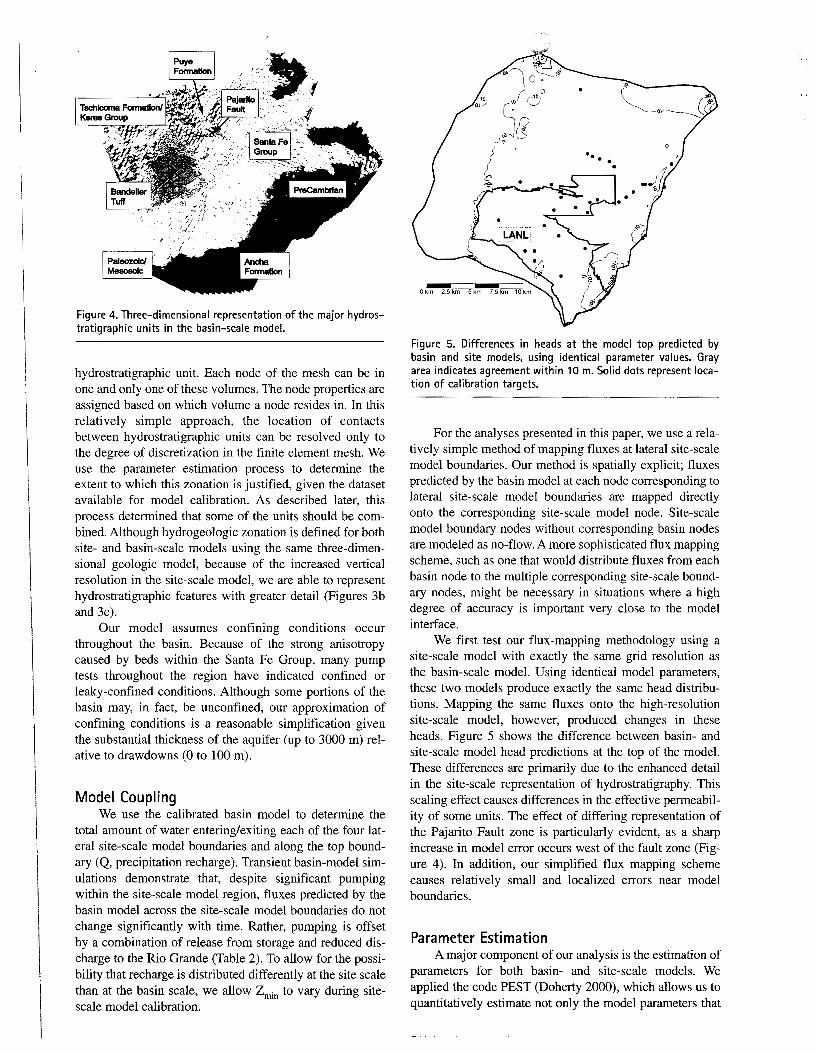
Hydrogeologic zones are defined by a three-dimen­sional geologic model for the basin (Carey et al. 1999). Zonation is defined primarily according to geologic fea­tures identified through field studies, geologic maps, inter­pretation of drillers logs, and geophysics (Vautaz et al. 1986; Baldridge et al. 1995; Smith et al. 1975; Kelley 1978; Manley 1979; Biehler et al. 1991; Ferguson et al. 1995; Dethier 1997). This process provides reasonably good con­trol on contacts between Santa Fe Group rocks and other units in the basin; however, subdividing the Santa Fe Group rocks (the largest unit in the basin) could not be accom­plished in this way. Therefore, we arbitrarily divided this unit into five broad geographic regions; later we test the validity of this subdivision using inverse modeling. The resulting model defines 23 geologic units, including two fault zones. A three-dimensional representation of the major units in the basin-scale model is shown in Figure 4.

Each node in the computational mesh is assigned to a unit according to its location relative to the three-dimen­sional hydrostratigraphic structure defined by the geologic model. Interpolation from the hydrostratigraphic model to the grid nodes is done by defining closed volumes for each

I

I

Figure 4. Three-dimensional representation of the major hydros­tratigraphic units in the basin-scale model.

hydrostratigraphic unit. Each node of the mesh can be in one and only one of these volumes. The node properties are assigned based on which volume a node resides in. In this relatively simple approach, the location of contacts between hydrostratigraphic units can be resolved only to the degree of discretization in the finite element mesh. We use the parameter estimation process to determine the extent to which this zonation is justified, given the dataset available for model calibration. As described later, this process determined that some of the units should be com­bined. Although hydrogeologic zonation is defined for both site- and basin-scale models using the same three-dimen­sional geologic model, because of the increased vertical resolution in the site-scale model, we are able to represent hydrostratigraphic features with greater detail (Figures 3b and 3c).

Our model assumes confining conditions occur throughout the basin. Because of the strong anisotropy caused by beds within the Santa Fe Group, many pump tests throughout the region have indicated confined or leaky-confined conditions. Although some portions of the basin may, in fact, be unconfined, our approximation of confining conditions is a reasonable simplification given the substantial thickness of the aquifer (up to 3000 m) rel­ative to drawdowns (0 to 100 m).

Model Coupling We use the calibrated basin model to determine the

total amount of water entering/exiting each of the four lat­eral site-scale model boundaries and along the top bound­ary (Q, precipitation recharge). Transient basin-model sim­ulations demonstrate that, despite significant pumping within the site-scale model region, fluxes predicted by the basin model across the site-scale model boundaries do not change significantly with time. Rather, pumping is offset by a combination of release from storage and reduced dis­charge to the Rio Grande (Table 2). To allow for the possi­bility that recharge is distributed differently at the site scale than at the basin scale, we allow zmin to vary during site­scale model calibration.

Figure 5. Differences in heads at the model top predicted by basin and site models, using identical parameter values. Gray area indicates agreement within 10m. Solid dots represent loca­tion of calibration targets.

For the analyses presented in this paper, we use a rela­tively simple method of mapping fluxes at lateral site-scale model boundaries. Our method is spatially explicit; fluxes predicted by the basin model at each node corresponding to lateral site-scale model boundaries are mapped directly onto the corresponding site-scale model node. Site-scale model boundary nodes without corresponding basin nodes are modeled as no-flow. A more sophisticated flux mapping scheme, such as one that would distribute fluxes from each basin node to the multiple corresponding site-scale bound­ary nodes, might be necessary in situations where a high degree of accuracy is important very close to the model interface.

We first test our flux-mapping methodology using a site-scale model with exactly the same grid resolution as the basin-scale model. Using identical model parameters, these two models produce exactly the same head distribu­tions. Mapping the same fluxes onto the high-resolution site-scale model, however, produced changes in these heads. Figure 5 shows the difference between basin- and site-scale model head predictions at the top of the model. These differences are primarily due to the enhanced detail in the site-scale representation of hydrostratigraphy. This scaling effect causes differences in the effective permeabil­ity of some units. The effect of differing representation of the Pajarito Fault zone is particularly evident, as a sharp increase in model error occurs west of the fault zone (Fig­ure 4). In addition, our simplified flux mapping scheme causes relatively small and localized errors near model boundaries.

Parameter Estimation A major component of our analysis is the estimation of

parameters for both basin- and site-scale models. We applied the code PEST (Doherty 2000), which allows us to quantitatively estimate not only the model parameters that

,,,.,,

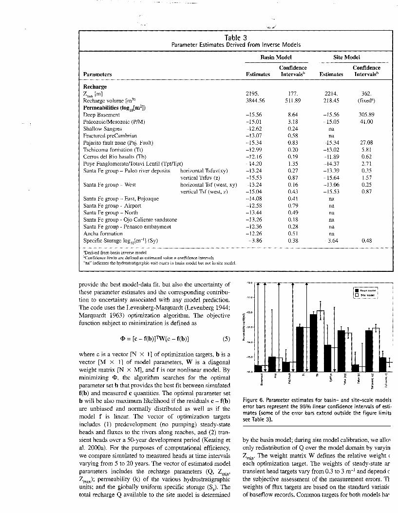
Table 3 Parameter Estimates Derived from Inverse Models

Parameters

Recharge zmin [m] Recharge volume [m3]

Permeabilities (log10[m2])

Deep Basement Paleozoic/Mesozoic (P/M) Shallow Sangres Fractured preCambrian Pajarito fault zone (Paj. Fault) Tschicoma formation (Tt) Cerros del Rio basalts (Tb) Puye Fanglomerateffotavi Lentil (Tpfffpt) Santa Fe group- Paleo river deposits horizontal Tsfuv(xy)

vertical Tsfuv (z) Santa Fe group -West horizontal Tsf (west, xy)

vertical Tsf (west, z) Santa Fe group- East, Pojoaque Santa Fe group -Airport Santa Fe group- North Santa Fe group - Ojo Caliente sandstone Santa Fe group - Penasco embayment Ancha formation Specific Storage log

10[m- 1] (Sy)

'Derived from basin inver<e model bConfidence limits are defined as estimated value ± confidence intervals. "na" indicates the hydrostratigraphic unit exists in basin model but not in site model.

provide the best model-data fit, but also the uncertainty of these parameter estimates and the corresponding contribu­tion to uncertainty associated with any model prediction. The code uses the Levenberg-Marquardt (Levenberg 1944; Marquardt 1963) optimization algorithm. The objective function subject to minimization is defined as

<P = [c- f(b)]1W[c- f(b)] (5)

where c is a vector [N X 1] of optimization targets, b is a vector [M X 1] of model parameters, W is a diagonal weight matrix [N X M], and f is our nonlinear model. By minimizing <P, the algorithm searches for the optimal parameter set b that provides the best fit between simulated f(b) and measured c quantities. The optimal parameter set b will be also maximum likelihood if the residuals c - f(b) are unbiased and normally distributed as well as if the model f is linear. The vector of optimization targets includes (1) predevelopment (no pumping) steady-state heads and fluxes to the rivers along reaches, and (2) tran­sient heads over a 50-year development period (Keating et al. 2000a). For the purposes of c.Jmputational efficiency, we compare simulated to measured heads at time intervals varying from 5 to 20 years. The vector of estimated model parameters includes the recharge parameters (Q, zrnin• zmax); permeability (k) of the various hydrostratigraphic units; and the globally uniform specific storage (Ss). The total recharge Q available to the site model is determined

Basin Model Site Model

Confidence Confidence Estimates Intervalsh Estimates Intervalsh

2195. 177. 2214. 362. 3844.56 511.89 218.45 (fixed a)

-15.56 8.64 -15.56 305.89 -15.01 3.18 -15.05 41.00 -12.62 0.24 na -13.07 0.58 na -15.34 0.83 -15.34 27.08 -12.99 0.20 -13.02 5.81 -12.16 0.19 -11.89 0.62 -14.20 1.35 -14.37 2.71 -13.24 0.27 -13.39 0.35 -15.53 0.87 -15.64 1.57 -13.24 0.16 -13.06 0.25 -15.04 0.43 -15.53 0.87 -14.08 0.41 na -12.58 0.79 na -13.44 0.49 na -13.26 0.18 na -12.36 0.28 na -12.26 0.51 na -3.86 0.38 -3.64 0.48

-16.0

" ,. ;; " ~ " ~ :;;:

~ ;;: ~ i ~ ! £ ~

Figure 6. Parameter estimates for basin- and site-scale models error bars represent the 95<¥o linear confidence intervals of esti· mates (some of the error bars extend outside the figure limits see Table 3).

by the basin model; during site model calibration, we allo1 only redistribution of Q over the model domain by varyin Zrnin· The weight matrix W defines the relative weight< each optimization target. The weights of steady-state ar transient head targets vary from 0.3 to 3 m-1 and depend c the subjective assessment of the measurement errors. Tl weights of flux targets are based on the standard variati< of base flow records. Common targets for both models ha'

I I I

I I

I

I "tl

"' 'iU :; E iii

c c .... N

c c

"'

u o Pre-development~ .1t. Transient

- -Perfect Fit N

c c M N

c c ;;;

c c ~

c c :::: . .;

/.

~ /

1500

/ /

0 /:'> 8 t~> • <* <)

¢ o O/o o<)-O

_:!;< 0,. 0

0;"'

1/Z _;

1700 1900 2100

Measured [m]

/ / ~

'/ /

/ /

/ /

/

v

2300 2500 2700

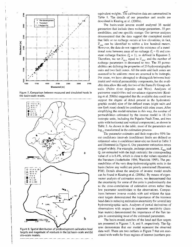
Figure 7. Comparison between measured and simulated heads in the basin-scale model.

<> -111.4 to -20

6. -20 to -10 0 -10 to -5 0 -5 to 5 • 5 to 10 .&. 10 to 20 • 20 to 200

<> -111.4 to -20 /':,. -20 to -10 0 -10 to -5 0 -5 to 5 • 5 to 10 A 10 to 20 + 20 to 200

0 km 5 km

a

0

b

Figure 8. Spatial distribution of predevelopment calibration head targets and magnitude of residuals in the (a) basin-scale and (b) site-scale models.

~4#.#'

equivalent weights. The calibration data are summarized in Table I. The details of our procedure and results are described in Keating et al. (2000a).

The basin-scale inverse model analyzed 38 model parameters that include three recharge parameters, 35 per­meabilities, and one specific storage. Our inverse analyses demonstrated that the data support the conceptual model that little or no recharge occurs at low elevations; in fact, zmin can be identified to within a few hundred meters. However, the data do not support the existence of a transi­tional zone between areas of no recharge (S = 0) and con­stant recharge fraction (S = I), as defined in Equation 2. Therefore, we set Zmax equal to Zmin' and the number of recharge parameters is decreased to two. The 35 perme­abilities are defining the properties of 23 hydrostratigraphic units and two fault zones. All the units and fault zones are assumed to be uniform; most are assumed to be isotropic . For some, we have attempted to distinguish between hori­zontal and vertical permeability components, but the avail­able data allow this only for two of the Santa Fe Group sub­units (Paleo river deposits and West). Analyses of parameter sensitivities and covariance eigenvectors (Keat­ing et al. 2000a) suggested that the available data could not support the degree of detail present in the hydrostrati­graphic model; nine of the defined zones (eight units and one fault zone) should be combined with other zones. After simplifying the model structure in this way, the number of permeabilities estimated by the inverse model is 18 (14 isotropic units, including the Pajarito Fault Zone, and two units with horizontal and vertical components), as shown in Table 3. As shown in the table, most of the parameters are log10 transformed in the estimation process.

The parameter estimates and their respective 95% lin­ear confidence intervals (confidence limits are defined as estimated value± confidence intervals) are listed in Table 3 and illustrated in Figure 6. Our parameter estimation errors ranged widely. For example, recharge parameters, Zmin and Q, are estimated with the high certainty; the corresponding value of a is 8.4%, which is close to the values reported in the literature (Anderholm 1994; Wasiolek 1995). The per­meabilities of the very deep hydrostratigraphic units in the basin (below any wells) are poorly constrained (Basement, P/M). Details about the analysis of inverse model results can be found in Keating et al. (2000a). By means of eigen­vector analysis of estimation errors, we demonstrated that the uncertainty for some of the units is predominantly due to the cross-correlations of estimation errors rather than low parameter sensitivities to the observations. Compar­isons between inverse models with and without the tran­sient targets demonstrated the importance of the transient head data in reducing estimation uncertainty for several key hydrostratigraphic units. Analyses of partial derivatives of observations with respect to parameter sensitivity (Jaco­bian matrix) demonstrated the importance of the flux tar­gets in constraining most of the estimated parameters.

The basin-model matches of the head and flux targets are presented in Figures 7, 8, and 9, respectively. The fig­ures demonstrate that our model represent the observed data well. There are two outliers in Figure 7 that are asso­ciated with wells far from regions of interest (northern por-

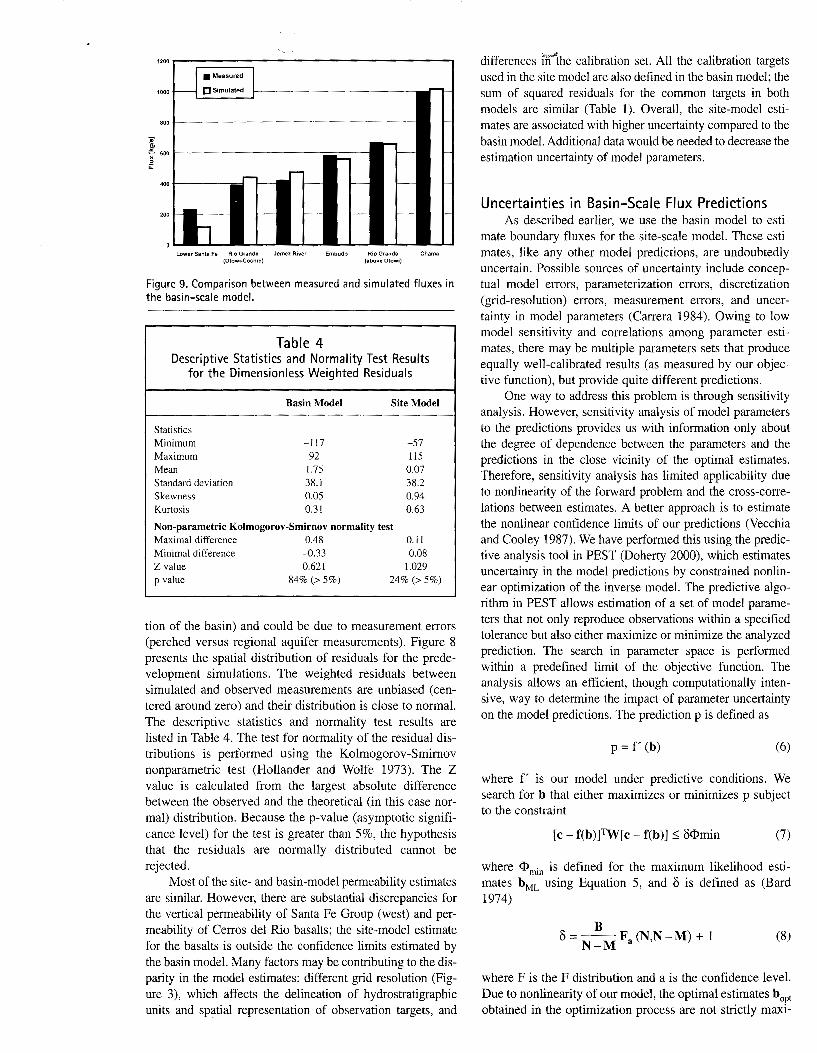
Lower Santa Fe Rio Grande Jemez River Embudo Rio Grande Chama (Otowi-Cochiti) (above otowi)

Figure 9. Comparison between measured and simulated fluxes in the basin-scale model.

Table 4 Descriptive Statistics and Normality Test Results

for the Dimensionless Weighted Residuals

Basin Model Site Model

Statistics Minimum -117 -57 Maximum 92 115 Mean 1.75 0.07 Standard deviation 38.1 38.2 Skewness 0.05 0.94 Kurtosis 0.31 0.63

Non-parametric Kolmogorov-Smirnov normality test Maximal difference 0.48 0.11 Minimal difference -0.33 -0.08 Z value 0.621 1.029 p value 84% (> 5%) 24% (> 5%)

tion of the basin) and could be due to measurement errors (perched versus regional aquifer measurements). Figure 8 presents the spatial distribution of residuals for the prede­velopment simulations. The weighted residuals between simulated and observed measurements are unbiased ( cen­tered around zero) and their distribution is close to normal. The descriptive statistics and normality test results are listed in Table 4. The test for normality of the residual dis­tributions is performed using the Kolmogorov-Smirnov nonparametric test (Hollander and Wolfe 1973). The Z value is calculated from the largest absolute difference between the observed and the theoretical (in this case nor­mal) distribution. Because the p-value (asymptotic signifi­cance level) for the test is greater than 5%, the hypothesis that the residuals are normally distributed cannot be rejected.

Most of the site- and basin-model permeability estimates are similar. However, there are substantial discrepancies for the vertical permeability of Santa Fe Group (west) and per­meability of Cerros del Rio basalts; the site-model estimate for the basalts is outside the confidence limits estimated by the basin model. Many factors may be contributing to the dis­parity in the model estimates: different grid resolution (Fig­ure 3), which affects the delineation of hydrostratigraphic units and spatial representation of observation targets, and

differences 11i'rhe calibration set. All the calibration targets used in the site model are also defined in the basin model; the sum of squared residuals for the common targets in both models are similar (Table 1). Overall, the site-model esti­mates are associated with higher uncertainty compared to the basin model. Additional data would be needed to decrease the estimation uncertainty of model parameters.

Uncertainties in Basin-Scale Flux Predictions As described earlier, we use the basin model to esti­

mate boundary fluxes for the site-scale model. These esti­mates, like any other model predictions, are undoubtedly uncertain. Possible sources of uncertainty include concep­tual model errors, parameterization errors, discretization (grid-resolution) errors, measurement errors, and uncer­tainty in model parameters (Carrera 1984). Owing to low model sensitivity and correlations among parameter esti­mates, there may be multiple parameters sets that produce equally well-calibrated results (as measured by our objec­tive function), but provide quite different predictions.

One way to address this problem is through sensitivity analysis. However, sensitivity analysis of model parameters to the predictions provides us with information only about the degree of dependence between the parameters and the predictions in the close vicinity of the optimal estimates. Therefore, sensitivity analysis has limited applicability due to nonlinearity of the forward problem and the cross-corre­lations between estimates. A better approach is to estimate the nonlinear confidence limits of our predictions (Vecchia and Cooley 1987). We have performed this using the predic­tive analysis tool in PEST (Doherty 2000), which estimates uncertainty in the model predictions by constrained nonlin­ear optimization of the inverse model. The predictive algo­rithm in PEST allows estimation of a set of model parame­ters that not only reproduce observations within a specified tolerance but also either maximize or minimize the analyzed prediction. The search in parameter space is performed within a predefined limit of the objective function. The analysis allows an efficient, though computationally inten­sive, way to determine the impact of parameter uncertainty on the model predictions. The prediction p is defined as

p = f' (b) (6)

where f' is our model under predictive conditions. We search for b that either maximizes or minimizes p subject to the constraint

[c- f(b)FW[c- f(b)] ::;; 8<l>min (7)

where <l>min is defined for the maximum likelihood esti­mates bML using Equation 5, and 8 is defined as (Bard 1974)

B 8 = --Fa (N,N- M) + 1

N-M (8)

where F is the F distribution and a is the confidence level. Due to nonlinearity of our model, the optimal estimates bopt

obtained in the optimization process are not strictly maxi-

.. 120 "

Inflow

80

40

T I I ...

~ e st I north west so~tn

-40

-80

Outflow -120

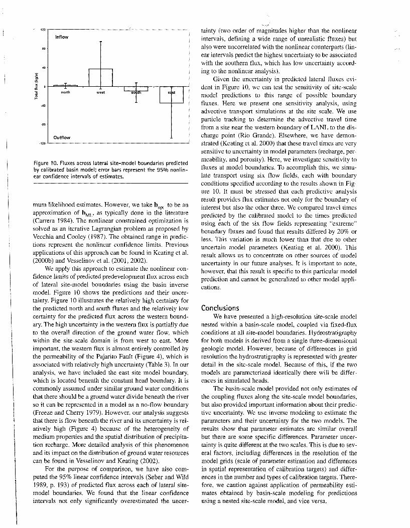
Figure 10. Fluxes across lateral site-model boundaries predicted by calibrated basin model; error bars represent the 95% nonlin­ear confidence intervals of estimates.

mum likelihood estimates. However, we take bopt to be an approximation of bML' as typically done in the literature (Carrera 1984). The nonlinear constrained optimization is solved as an iterative Lagrangian problem as proposed by Vecchia and Cooley (1987). The obtained range in predic­tions represent the nonlinear confidence limits. Previous applications of this approach can be found in Keating et a!. (2000b) and Vesselinov eta!. (2001, 2002).

We apply this approach to estimate the nonlinear con­fidence limits of predicted predevelopment flux across each of lateral site-model boundaries using the basin inverse model. Figure 10 shows the predictions and their uncer­tainty. Figure 10 illustrates the relatively high certainty for the predicted north and south fluxes and the relatively low certainty for the predicted flux across the western bound­ary. The high uncertainty in the western flux is partially due to the overall direction of the ground water flow, which within the site-scale domain is from west to east. More important, the western flux is almost entirely controlled by the permeability of the Pajarito Fault (Figure 4), which is associated with relatively high uncertainty (Table 3). In our analysis, we have included the east site model boundary, which is located beneath the constant head boundary. It is commonly assumed under similar ground water conditions that there should be a ground water divide beneath the river so it can be represented in a model as a no-flow boundary (Freeze and Cherry 1979). However, our analysis suggests that there is flow beneath the river and its uncertainty is rel­atively high (Figure 4) because of the heterogeneity of medium properties and the spatial distribution of precipita­tion recharge. More detailed analysis of this phenomenon and its impact on the distribution of ground water resources can be found in Vesselinov and Keating (2002).

For the purpose of comparison, we have also com­puted the 95% linear confidence intervals (Seber and Wild 1989, p. 193) of predicted flux across each of lateral site­model boundaries. We found that the linear confidence intervals not only significantly overestimated the uncer-

tainty (two order of magnitudes higher than the nonlinear intervals, defining a wide range of unrealistic fluxes) but also were uncorrelated with the nonlinear counterparts (lin­ear intervals predict the highest uncertainty to be associated with the southern flux, which has low uncertainty accord­ing to the nonlinear analysis).

Given the uncertainty in predicted lateral fluxes evi­dent in Figure 10, we can test the sensitivity of site-scale model predictions to this range of possible boundary fluxes. Here we present one sensitivity analysis, using advective transport simulations at the site scale. We use particle tracking to determine the advective travel time from a site near the western boundary of LANL to the dis­charge point (Rio Grande). Elsewhere, we have demon­strated (Keating et a!. 2000) that these travel times are very sensitive to uncertainty in model parameters (recharge, per­meability, and porosity). Here, we investigate sensitivity to fluxes at model boundaries. To accomplish this, we simu­late transport using six flow fields, each with boundary conditions specified according to the results shown in Fig­ure 10. It must be stressed that each predictive analysis result provides flux estimates not only for the boundary of interest but also the other three. We compared travel times predicted by the calibrated model to the times predicted using each of the six flow fields representing "extreme" boundary fluxes and found that results differed by 20% or less. This variation is much lower than that due to other uncertain model parameters (Keating et a!. 2000). This result allows us to concentrate on other sources of model uncertainty in our future analyses. It is important to note, however, that this result is specific to this particular model prediction and cannot be generalized to other model appli­cations.

Conclusions We have presented a high-resolution site-scale model

nested within a basin-scale model, coupled via fixed-flux conditions at all site-model boundaries. Hydrostratigraphy for both models is derived from a single three-dimensional geologic model. However, because of differences in grid resolution the hydrostratigraphy is represented with greater detail in the site-scale model. Because of this, if the two models are parameterized identically there wiii be differ­ences in simulated heads.

The basin-scale model provided not only estimates of the coupling fluxes along the site-scale model boundaries, but also provided important information about their predic­tive uncertainty. We use inverse modeling to estimate the parameters and their uncertainty for the two models. The results show that parameter estimates are similar overall but there are some specific differences. Parameter uncer­tainty is quite different at the two scales. This is due to sev­eral factors, including differences in the resolution of the model grids (scale of parameter estimation and differences in spatial representation of calibration targets) and differ­ences in the number and types of calibration targets. There­fore, we caution against application of permeability esti­mates obtained by basin-scale modeling for predictions using a nested site-scale model, and vice versa.

We have applied a robust (although computationally intensive) method to evaluate the uncertainty in our basin­scale model predictions of fluxes to the site-scale model. This method is preferable to conventional sensitivity analy­sis because it explicitly considers uncertainty in all param­eters and results are limited to combinations of model parameters that fall within specified model calibration cri­teria. Through this exercise, we have determined that fluxes to some lateral site-model boundaries are quite well con­strained by basin-model predictions; however, other lateral boundaries are far more uncertain. Site-scale model predic­tions of advective travel times are relatively insensitive to the uncertainty in these boundary fluxes; therefore, other sources of uncertainty should be given higher priority for future work.

Future work on the coupling of basin- and local-scale inverse models will include more rigorous analysis of prop­agation of uncertainty between the models, and evaluation of not only prediction but also estimation uncertainty in the local-scale inverse model due to uncertainty in the coupling predicted by the basin-scale inverse model.

Acknowledgments This work has been supported by the Department of

Energy and the Los Alamos National Laboratory Hydroge­ologic Characterization Program. We are grateful for con­tributions by Greg Cole, Bill Carey, and Carl Gable in development of the hydrostratigraphic framework model and computational grids.

References Anderholm, S.K. 1994. Ground-water recharge near Santa Fe,

north-central New Mexico. U.S. Geological Survey Water Resources Investigations Report 94-4078.

Anderson, M., and W.W.Woessner. 1992. Applied Groundwater Modeling. San Diego: Academic Press.

Baldridge, W.S., J.F. Ferguson, L.W. Braile, B. Wang, K. Eck­hardt, D. Evans, C. Schultz, B. Gilpin, G.R. Jiracek, and S. Biehler. 1995. The western margin of the Rio Grande Rift in northern New Mexico: An aborted boundary? GSA Bulletin 105, 1538-1551.

Bard, M. 1974. Nonlinear Parameter Estimation. New York: Academic Press.

Biehler, S.J., J. Ferguson, W.S. Baldridge, G.R. Jiracek, J.L. Aldern, M. Martinez, R. Fernandez, J. Romo, B. Gilpin, and L.W. Braille. 1991. A geophysical model of the Espanola Basin, Rio Grande Rift, New Mexico. Geophysics 56, no. 3: 340-353.

Bowen, B.M. 1992. Los Alamos climatology summary including latest normals from 1961-1990. Los Alamos National Lab­oratory Report LA-12232-MS. http://lib-www.lanl.gov/la­pubs/OO 194103 .pdf.42.

Brian, C., and P.E.Wilson.1997. Water use by categories in New Mexico counties and river basins, and irrigated acreage in 1995. New Mexico State Engineer Office, Technical Report, Santa Fe, New Mexico.

Carey, B., G.Cole, C. Lewis, F. Tsai, R. Warren, and G. Wolde­Gabriel. 1999. Revised site-wide geologic model for Los Alamos National Laboratory. Los Alamos National Labora­tory Report LA-UR-00-2056. http://lib-www.lanl.gov/la­pubs/00393599.pdf.

Carrera, J. 1984. Estimation of aquifer parameters under transient and steady state conditions. Ph.D. thesis, University of Ari­zona, Tucson, Arizona.

Coon, L.M., and T.E. Kelly. 1984. Regional hydrogeology and the effect of structural control and the flow of ground water in the Rio Grande trough, northern New Mexico. New Mex­ico Geological Society Guidebook, 35th Field Conference, Rio Grande Rift, Northern New Mexico, 241-244.

Cordell, L. 1979. Gravimetric expression of graben faulting in Santa Fe County and the Espanola Basin, New Mexico. New Mexico Geologic Society Guidebook, 30th Field Con­ference, Santa Fe County, 59-64.

Daniel B. Stephens & Associates Inc. 1994. Santa Fe County water resource inventory. Santa Fe, New Mexico: Daniel B. Stephens and Associates Inc.

Dethier, D.P. 1997. Geology of White Rock quadrangle, Los Alamos and Santa Fe counties, New Mexico. New Mexico Bureau of Mines & Mineral Resources Geologic Map.

Doherty, J. 2000. PEST: Model Independent Parameter Estima­tion. Brisbane, Australia: Watermark Computing.

Ferguson, J.F., W.S. Baldridge, L.W. Braile, S. Biehler, B. Gilpin, and G.R. Jiracek. 1995. Structure of the Espanola Basin, Rio Grande Rift, New Mexico, from SAGE seismic and gravity data. New Mexico Geological Society Guidebook, 46th Field Conference, Geology of the Santa Fe Region, 105-109.

Frenzel, P.F. 1995. Geohydrology and simulation of ground­water flow near Los Alamos, north central New Mexico. U.S. Geological Survey Water Resources Investigations Report 95-4091.

Freeze, R.A., and J.A. Cherry. 1979. Groundwater. New Jersey: Prentice Hall.

Giudici, M., G. Parravicini, G. Ponzini, E. Romano, and D. Villa. 2001. Nested models to simulate groundwater flow at dif­ferent scales. Geophysical Research Abstracts 3, 2086.

Hearne, G.A. 1985. Mathematical model of the Tesuque aquifer system underlying Pojoaque River Basin and vicinity, New Mexico. U.S. Geological Survey Water-Supply Paper 2205.

Hollander, M., and D.A.Wolfe. 1973. Nonparametric Statistical Methods. New York: John Wiley & Sons.

Hunt, R., J. Steuer, M. Mansor, and T. Bullen. 2001. Delineating a recharge area for a spring using numerical modeling, Monte Carlo techniques, and geochemical investigation. Ground Water 39, no. 5: 702-712.

Keating, E.H., and J.M. Bahr. 1998. Using reactive solutes to constrain groundwater flow models at a site in northern Wisconsin. Water Resources Research 34, no. 12: 3561-3571.

Keating, E.H., E. Kwicklis, V. Vesselinov, A. Idar, Z. Lu, G. Zyvoloski, and M. Witkowski. 2000a. A regional flow and transport model for groundwater at Los Alamos National Laboratory. Los Alamos National Laboratory Report LA­UR-01-2199, http://lib-www.lanl.gov/la-pubs/00818241.pdf

Keating, E.H., J. Doherty, and V. Vesselinov. 2000b. Approaches to quantifying uncertainty in flow directions in the regional aquifer beneath the Pajarito Plateau, northern New Mexico Supplement to EOS Transactions 81, no. 48: F511.

Keating, E.H., E. Kwicklis, M. Witkowski, and T. Ballantine 1999. A regional flow model for the regional aquife beneath the Pajarito Plateau. Los Alamos National Labora tory Report LA-UR-00-1029.

Keating, E.H., and V.V. Vesselinov. 2001. A comparison of tw approaches to modeling capture zones at the site-seal( Adaptive mesh refinement within a basin-scale model an site-scale/basin-scale model coupling. Eos. Trans. AGU 8: no. 47, Abstract H22D-0383.

Kelley, V.C. 1978. Geology of the Espanola Basin. New Mexic Bureau of Mines and Mineral Resources Map.

Kernodle, J.M.D.P.M., and C.R. Thorn. 1995. Simulation ground-water flow in the Albuquerque Basin, central Nc Mexico, 1901-1994, with projections to 2020. USC Water-Resources Investigation Report 94-4251.

Los Alamos National Laboratory. 1998. Hydrogeologic Wo, plan. Environment, Safety, and Health Division, LANL, I Alamos, New Mexico, LAUR 01-6511.

\

Leake, S., P. Lawson, M. Lilly, and D~"mar. 1998. Assignment of boundary conditions in embedded ground water flow models. Ground Water 36, no. 4: 621-625.

Levenberg, K.A. 1944. A method for the solution of certain non­linear problems in least squares. Quarterly of Applied Math­ematics 2, 164-168.

Manley, K. 1979. Stratigraphy and structure of the Espanola Basin, Rio Grande Rift, New Mexico. In Rio Grande Rift: Tectonics and Magmatism, ed. R.E. Riecker, 71-86. Ameri­can Geophysical Union Special Publication.

Marquardt, D.W. 1963. An algorithm for least-squares estimation of nonlinear parameters. Journal of the Society of Industrial and Applied Mathematics 11, no. 3:431-441.

McAda, D.P., and M. Wasiolek. 1988. Simulation of the regional geohydrology of the Tesuque aquifer system near Santa Fe, New Mexico. U.S. Geological Survey Water Resources Investigations Report 87-4056.

Meier, P.M., J. Carrera, and X. Sanchez-Vila. 1999. A numerical study on the relationship between transmissivity and spe­cific capacity in heterogeneous aquifers. Gn;nmd Water 37, no. 4:611-617

Purtymun, W.D. 1984. Hydrologic characteristics of the main aquifer in the Los Alamos area: Development of ground water supplies. Los Alamos National Laboratory Report LA-995.

Purtymun, W.D., and S. Johansen. 1974. General geohydrology of the Pajarito Plateau. New Mexico Geologic Society Guidebook, 25th Field Conference.

Purtymun, W.D., A.K. Stoker, and S.G. McLin. 1995. Water sup­ply at Los Alamos during 1993. Los Alamos National Lab­oratory Report LA-12951-PR.

Seber, G.A.F., and C.J. Wild. 1989. Nonlinear Regression. New York: John Wiley & Sons.

Smith, R.L., R.A. Bailey, and C.S. Ross. 1975. Geologic map of the Jemez Mountains, New Mexico. U. S. Geological Sur­vey Miscellaneous Investigations Series Map.

Spiegel, Z., and B. Baldwin. 1963. Geology and water resources of the Santa Fe area. U.S. Geological Survey Water-Supply Paper 1525.

Tiedeman, C.R., J.M. Kernodle, and D.P. McAda. 1998. Appli­cation of nonlinear-regression methods to a ground-water flow model of the Albuquerque Basin, New Mexico. U.S. Geological Survey Water-Resources Investigations Report 98-4172.90.

Trease, H., D. George, C.W. Gable, J. Fowler, A. Kuprat, and A. Khamyaseh. 1996. The X3D grid generation system. In Numerical Grid Generation System in Computational Fluid Dynamics and Related Fields, ed. B.K. Soni, J.F. Thomp­son, H. Hausser, and P.R. Eiseman. 1129. Starkville, Missis­sippi: Mississippi State University.

U.S. Geological Survey. 1997. WATSTORE database.

U.S. Geological SurveMOOI. Surface-Water Data for USA. http://water.usgs.gov/nwis/sw.

Vautaz, F.D., F. Goff, C. Fouillac, and J.Y. Calvez. 1986. Isotope geochemistry of thermal and nonthermal waters in the Valles Caldera, Jemez Mountains, northern New Mexico. Journal of Geophysics Research 91, 1835-1853.

Vecchia, A.V., and R.L. Cooley. 1987. Simultaneous confidence and prediction intervals for nonlinear regression models with application to a groundwater flow model. Water Resources Research 23, no. 7: 1237-1250.

Vesselinov, V.V., E.H. Keating, and J. Doherty. 2001. Analysis of uncertainty in model predictions of flow and transport in the Espanola Basin regional aquifer, northern New Mexico. Eos. Trans. AGU 82, no. 47, Abstract Hl2D-0329.

Vesselinov, V.V., and S. Neuman. 2001. Numerical inverse inter­pretation of single-hole pneumatic tests in unsaturated frac­tured tuff. Ground Water 39, no. 5: 685-695.

Vesselinov, V.V., and E.H.Keating. 2002. Analysis of capture zones of the Buckman Wellfield and a proposed new hori­zontal collector well north of the Otowi Bridge, Los Alamos National Laboratory Report LA-UR-02-2750.

Vesselinov, V.V., E.H. Keating, and G.A. Zyvoloski. 2002. Analysis of model sensitivity and predictive uncertainty of capture zones in the Espanola Basin regional aquifer, north­ern New Mexico. International Conference Mode/CARE 2002 Calibration and Reliability in Groundwater Model­ling: A Few Steps Closer to Reality, Prague, Czech Repub­lic, 17-20.

Walker, D., and B. Gylling. 1998. Site-scale groundwater flow modelling of Aberg. Swedish Nuclear Fuel and Waste Man­agement Company Technical Report, TR-98-23.167.

Ward, D.S., D.R. Buss, J.W. Mercer, and S.S. Hughes. 1987. Evaluation of a groundwater corrective action at the Chem­Dyne hazardous waste site using a telescopic mesh refine­ment modeling approach. Water Resources Research 23, no. 4: 603-617.

Wasiolek, M. 1995. Subsurface recharge to the Tesuque aquifer system from selected drainage basins along the western side of the Sangre de Cristo Mountains near Santa Fe, New Mex­ico. U.S. Geological Survey Water-Resources Investigations Report 94-4072.

Zyvoloski, G., E. Kwicklis, A. Eddebbarh, B. Arnold, C. Faunt, and B.A. Robinson. 2002. The site-scale saturated-zone flow model for Yucca Mountain: Calibration of different conceptual models and their impact on transport. Journal of Contaminant Hydrology, in press.

Zyvoloski, G.A., B.A. Robinson, Z.V. Dash, and L.L. Trease. 1997. Summary of the models and methods for the FEHM application: A finite-element heat- and mass-transfer code. Los Alamos National Laboratory Report LA-13306-MS.