Embed Size (px)
Citation preview
Coupled-resonator Optical Waveguides
and Multiplexed Solitons
Engineering linear and nonlinear periodicphenomena for optical communications
Shayan Mookherjea
In partial fulfillment of the requirements forthe degree of Doctor of Philosophy at theCalifornia Institute of Technology, June 2003
Defended Sept. 6, 2002, Revised Apr. 9, 2003.
ii
Copyright 2003
California Institute of Technology
All rights reserved
Figs 1.1 and 1.2 were generated by the author using data obtained from the
software package Translight written by Andrew L. Reynolds at the Photonic Band
Gap Materials Research Group within the Optoelectronics Research Group of the
Department of Electronics and Electrical Engineering, the University of Glasgow.
Translight is based on the Transfer Matrix Method developed by J. Pendry,
P. M. Bell, A. J. Ward, and L. M. Moreno of the Imperial College, London.
iii
Thesis Committee
Amnon Yariv
Martin and Eileen Summerfield Professor of Applied Physics
Thomas A. Tombrello
William R. Kenan, Jr., Professor and Professor of Physics
Donald S. Cohen
Charles Lee Powell Professor of Applied Mathematics
David B. Rutledge
Kiyo and Eiko Tomiyasu Professor of Electrical Engineering
Axel Scherer
Bernard A. Neches Professor of Electrical Engineering,
Applied Physics and Physics

iv
v
Practically, we are not interested in exact transmission when we havea continuous source, but only in transmission to within a certain tolerance.
—C. E. Shannon, Bell Syst. Tech. J., 27, pp. 379–423, 623–656 (1948).
We observe from Fig. 1.1 thatcommunication system architecture centers or pivots around the
communications channel ... Modeling the effects of the physical channelon the propagating electromagnetic field in different frequency bands
and under various scenarios is a continuous and ongoing task.
—M. K. Simon, S. M. Hinedi and W. C. Lindsey DigitalCommunication Techniques, Prentice Hall (Englewood Cliffs, NJ, 1995).

vi
vii
Preface
The brevity of life does not allow us the luxury of spending time on problems which will lead to nonew results.
—–L. D. Landau, as quoted by E. M. Lifshitz in L. D. Landau and E. M. Lifshitz,Mechanics, Vol. 1 of Course of Theoretical Physics, Pergamon Press (Oxford, 1976).
This thesis addresses two topics in lightwave communication systems—increasing the
bit rate of data transmission, and finding a way to temporarily store information-
carrying optical pulses in compact semiconductor devices. The former identifies a
way to utilize existing (nonlinear) transmission phenomena to advantage in sending
information across optical fiber, and the latter is a proposal for a class of devices that
are frontline components in packet-switched optical networks.
The fundamental format for carrying information is an optical pulse, a localized
packet of electromagnetic energy. The output light from a laser, at a particular carrier
optical frequency, is turned on and off at a particular rate (amplitude modulation1)
to create a train of pulses which represents the information in a sequence of bits. The
frequency (Fourier) spectrum of an amplitude modulated signal contains a narrow
band of frequency components around the carrier frequency; the faster the rate of
modulation, the greater the spectral width of this band.
It is necessary that this band of frequencies fits within the “transparency window”
of the transmission medium. Fibers made of high-purity silica have a very wide range
of frequencies available for carrying information, and therefore, the modulation rate
can be quite high. It is, in fact, other practical issues that place a lower limit on the
minimum pulse width—a few hundred femtoseconds in long-distance communications.
A minimum pulse width means that the maximum spread of the modulation band
1The overwhelming majority of practical schemes for optical communications use amplitude mod-ulation (on-off keying), although other forms of modulation (frequency or phase) have been investi-gated.
viii
around the center (carrier) frequency is restricted, and the available spectrum of the
optical fiber outside this band is not utilized.
For higher data-rate communications, a number of different lasers with different
center frequencies can be modulated simultaneously2, so that more of the available
transmission channel bandwidth is used efficiently. A simple picture of a digital
transmission format is the so-called wavelength-division multiplexing (WDM) over
time-division multiplexing (TDM): the presence of a pulse of light at a particular
frequency (wavelength) in a particular timeslot signifies a “one” and whose absence
then signifies a “zero.” The successful operation of a high-speed multichannel com-
munication system depends on the degree to which the noise of the system can be
compensated for, and the principal sources of noise in optical channels include the
dispersion of the fiber, effects of nonlinearities in the dielectric material that com-
prises the fiber, and the noise added by optical amplifiers. Conventional systems try
to minimize the effect of dispersion and of the nonlinearities; the recent development
of optical solitons makes it possible to design a system that utilizes dispersion and
nonlinearity constructively.
Prof. Amnon Yariv has always made himself available for counsel, and has gener-
ously let me define my own thesis, based on topics I found promising and meaningful.
My experiences associated with his research group will be invaluable in the years
ahead. Profs. Don Cohen and Bruno Crosignani have been valuable collaborators
in aspects of this work, particularly deserving of acknowledgment in an environment
where effective scientific collaboration is difficult. Profs. Tom Tombrello, Don Cohen,
Dave Rutledge, and Axel Scherer graciously served on my thesis committee and have
been a source of continuing help and advice over many years.
At MIT, Prof. Vincent Chan supported my research on optical networks, a col-
laboration and friendship that extended even when I returned to Caltech. The en-
couragment of Profs. Hermann Haus and Erich Ippen was a source of inspiration. I’d
also like to take this opportunity to thank a few other outstanding teachers I’ve had
the privilege of learning from: Profs. Jim Fujimoto, Glen George, Jin Au Kong, Bob
McEliece, and Mark Wise.
2Or a number of designated wavelengths can be filtered from a single source of sufficient band-width.
ix
Historical outline: In January 2001, Yi Li, with whom I shared an office at the
time, told me of his conversations with Prof. Yariv on the frozen-light experiments
performed by the Harvard groups (Hau and Lukin), which led to my interpreting their
approach based on electromagnetically induced transparency as phenomenologically
very similar to holography (February 1, 2001, and in later conversations with Lene
Hau, June 6, 2002). At that time, we weren’t quite sure how to translate the slow-
light phenomenology to the optical domain. A month later (March 14, 2001), Yong
Xu told me about his idea of using defect states pulled outside a CROW band to trap
light propagating in the CROW band. Although this wasn’t in itself a solution to
our problem, it seemed plausible that combining the reduction in the group velocity
of light propagating in a CROW band with the photorefractive process would lead
to interesting new applications. But there were few studies of pulse propagation in
photonic crystal waveguides at that time beyond that of numerical simulations, and
none of nonlinear processes such as the photorefractive effect in such waveguides.
We are now able to characterize pulse propagation in CROWs not only in the
linear dispersion approximation—as is most practical for applications based on index
gratings, e.g., holography—but using the complete (nonlinear) dispersion relationship.
This led to our prediction and analyses of a class of super-resonant modes in CROWs
comprised of χ(3) material, which are essentialy Schrodinger solitons but with zero
group velocity—they remain spatially frozen to a finite section of the waveguide.
My work on solitons in optical fibers began soon after I joined Caltech (July
2000). There are interesting analogies between the diffraction of a Gaussian beam in
a rotationally symmetric quadratic index medium and the propagation of a Gaussian
pulse in the presence of the Kerr effect. Some of the analogies cannot be explained
algebraically, i.e., the ABCD matrix translation rules fail, but topological arguments
are very effective (January 2001, following a suggestion by Prof. D. S. Cohen). Inas-
much as conformal mappings have become an important tool in waveguide design,
geometric arguments may offer a new way to design nonlinear optical transmission
links.
We have analyzed the Hamiltonian approach to designing a nonlinearly multi-
plexed dispersion-managed soliton transmission communication system (June 2001).
Breathing pulse shapes traverse closed orbits in phase space, and therefore, we may
identify different trajectories with different codes to achieve higher channel capacity
than possible in linear channels.
x
My closest collaborators, George T. Paloczi and Dr. Yanyi Huang, are particularly
deserving of thanks for their friendship, and sharing in both the excitement and the
difficulties of research in exciting new fields as part of the Yariv Group at Caltech.
I’m very grateful for the continued support and enthusiasm of my office mates, Prof.
Avishay Eyal, Yi Li, Joyce Poon, and Dr. Koby Scheuer. John Choi, Will Green,
Dr. Reginald Lee, George Ouyang, Shervin Taghavi, and Dr. Yong Xu contributed
to our research, activities and conversations. Past and present students of Prof.
Axel Scherer’s group, including Dr. Marco Loncar, Prof. Oskar Painter, Prof. Jelena
Vuckovic, and Tomo Yoshie, have made numerous helpful suggestions. Dr. Zhiwen
Liu’s expertise on photorefractive holography was useful in designing the experiments
on ultrafast photorefractive holography. Dr. Bill Marshall participated in some of our
discussions on the effects of noise on the nonlinear propagation of breathers. More
than once, Daniel Katz helped as a friendly and informal mathematical consultant.
To them and to the many others who have talked to me about their own work, and
kept me interested in research problems beyond my own, my sincere thanks.
Andre Tkacenko has been a great guy to hang out with since our days as under-
grads at Caltech, and to share a love of mathematics, LATEX, cool computers, and the
finer aspects of life, cars, and electrical engineering. Salil Parikh will make his mil-
lions in matter of months now, and then we’ll hang out in Vegas—or Portland—like
we’ve been promising to. Cheewei Wong and Shashi Murthy have been wonderful
friends, and are a perennial excuse to go to Boston anytime, even in winter. Dr. John
Cortese’s advice on physics, mathematics, and electrical engineering over many years
is much appreciated. And, more than these few words say, a special note of thanks to
Joyce Poon for her friendship and support. I’d also like to acknowledge the friendly
and cheerful assistance of Linda Dosza, Ling Lin, Irene Loera, Connie Rodriguez, and
Michelle Vine.
This work is dedicated, with all my love, to my parents, who through their lives
have given and taught me far more than I could have ever wished. No words can
begin to repay the debt of gratitude I owe them.
Shayan Mookherjea
Pasadena, CA
xi
Abstract
Whether over micron-long or kilometer-long distances, periodic phenomena can strongly
affect both the propagation and the confinement of optical pulses. Periodicities can be
engineered through the structural design of optical waveguides, or they may manifest
self-consistently from induced nonlinear polarizations. In light of recent developments
in fabrication technologies for semiconductor waveguides, polymeric materials, and
optical fiber, we show that both strongly- and weakly-nonlinear channels are promis-
ing for new devices and systems in optical communications. This thesis proposes
and discusses applications of guided wave periodicities in the framework of photonic
crystals (coupled-resonator optical waveguides as well as transverse Bragg resonance
waveguides and amplifiers), nonlinear phenomena in photorefractive semiconductors,
and the nonlinear evolution of temporal solitons in dispersion-managed fibers.
Coupled-resonator optical waveguides (CROWs) are composed of a periodic array
of electromagnetic resonators, typically on the micron or sub-micron length scales. A
photon in such a waveguide sees a periodic potential, and according to the Floquet-
Bloch theorems, has a wavefunction that reflects this periodicity. CROWs have a
unique dispersion relationship compared to other semiconductor waveguides, and can
be used to slow down the speed of propagation, enhance nonlinear interactions such as
second-harmonic generation and four-wave mixing, and form frozen soliton-type field
distributions that use the optical Kerr nonlinearity to stabilize themselves against
decay via adjacent-resonator or waveguide-resonator coupling.
In optical fibers that possess the optical Kerr nonlinearity in addition to group-
velocity dispersion, it is possible to propagate pulses with envelopes that “breathe”
with distance, typically at kilometer or longer length scales. Such waveforms are
characterized by a set of parameters—e.g., amplitude, chirp, etc.—that vary in a
periodic manner as the pulse propagates. Borrowing an idea from field theory, e.g., of
classical pendulums, or quantum-mechanical elementary particles, the pulse envelope
xii
may be viewed as a particle traversing a trajectory in a phase space defined by
its characteristic parameters. Distinct, non-overlapping trajectories are assigned as
symbols of a multilevel communication code. Since it is the periodicity, arising from
the Kerr nonlinearity, that generates this diversity in phase-space, there is no analog
of this multiplexed system in linear optical transmission links. The overall bit-rate
can be improved several fold above the current limits.
xiii
Contents
1 Fundamentals 15
1.1 Pulse propagation in a linear waveguide . . . . . . . . . . . . . . . . . 17
1.2 Field evolution in a linear structure . . . . . . . . . . . . . . . . . . . 18
1.3 Nonlinear pulse propagation: solitons . . . . . . . . . . . . . . . . . . 19
1.4 Quasi-solitons and breathers . . . . . . . . . . . . . . . . . . . . . . . 23
1.5 Photonic crystals . . . . . . . . . . . . . . . . . . . . . . . . . . . . . 24
2 Linear propagation in the tight-binding approximation 33
2.1 Eigenmodes and “coupled mode theory” . . . . . . . . . . . . . . . . 33
2.2 The tight-binding approximation . . . . . . . . . . . . . . . . . . . . 36
2.2.1 Dispersion relationship . . . . . . . . . . . . . . . . . . . . . . 37
2.3 Pulse propagation . . . . . . . . . . . . . . . . . . . . . . . . . . . . . 42
2.4 Frequency, space, and time sampling . . . . . . . . . . . . . . . . . . 46
2.4.1 K-space representation of Eq. (2.24) . . . . . . . . . . . . . . 48
2.5 Linear pulse propagation: Bloch waves . . . . . . . . . . . . . . . . . 49
2.6 Using the full dispersion relationship . . . . . . . . . . . . . . . . . . 52
3 Two-pulse nonlinear interactions 61
3.1 Description of a pulse with an envelope in a CROW . . . . . . . . . . 62
3.2 Representation in the Bloch form . . . . . . . . . . . . . . . . . . . . 65
3.3 Second harmonic generation: formulation . . . . . . . . . . . . . . . . 67
3.4 Solutions to the SHG equations . . . . . . . . . . . . . . . . . . . . . 71
4 Holography and four-pulse mixing 75
4.1 Applications: Nonlinear Delay Lines . . . . . . . . . . . . . . . . . . . 80
4.2 Picosecond dynamics of photorefractive gratings in GaAs . . . . . . . 84
xiv
5 The Kerr effect and super-resonant modes 89
5.1 Formulation of the nonlinear propagation problem . . . . . . . . . . . 90
5.2 The stationary super-resonant mode . . . . . . . . . . . . . . . . . . . 92
6 Dispersion-managed solitons and breathers 99
6.1 Lagrangian and Hamiltonian formulation . . . . . . . . . . . . . . . . 101
6.1.1 Existence of breathing solutions for third-order dispersion . . . 106
6.2 Phase-plane analysis . . . . . . . . . . . . . . . . . . . . . . . . . . . 107
6.3 Dispersion maps including third-order dispersion . . . . . . . . . . . . 113
7 Multilevel communications in nonlinear fibers 119
7.1 Formulation . . . . . . . . . . . . . . . . . . . . . . . . . . . . . . . . 120
7.2 Analytical framework . . . . . . . . . . . . . . . . . . . . . . . . . . . 121
7.3 Multiple orbits and multiplexing . . . . . . . . . . . . . . . . . . . . . 126
7.3.1 RMS radius of the random walk in the phase plane . . . . . . 132
7.4 Gordon-Haus timing jitter . . . . . . . . . . . . . . . . . . . . . . . . 135
7.5 Comments . . . . . . . . . . . . . . . . . . . . . . . . . . . . . . . . . 139
7.5.1 Optimum amplifier gain for fixed total distance . . . . . . . . 141
8 Space-time analogies in pulse propagation 145
8.1 Gaussian beam diffraction and pulse propagation . . . . . . . . . . . 147
8.2 The ABCD formalism for Gaussian pulses . . . . . . . . . . . . . . . 149
8.3 DM soliton transmission experiment . . . . . . . . . . . . . . . . . . . 157
8.4 Hermite-Gaussian basis . . . . . . . . . . . . . . . . . . . . . . . . . . 162
8.5 Geometric analogies . . . . . . . . . . . . . . . . . . . . . . . . . . . . 164
A Superstructure gratings 175
B Watson’s criterion and Gaussian envelopes 177
C Outline of the proof of the Hermiticity of H 179
D Nonlinear polarization for SHG 181
E Period of orbits in the phase plane 185
Chapter 1
Fundamentals
It is my experience that the direct derivation of many simple,well-known formulae from first principles is not easy to find in print.
The original papers do not follow the easiest path, the authors of reviewsfind the necessary exposition too difficult—or beneath their dignity—
and the treatises are too self-conscious about completeness and rigour.
—J. M. Ziman, Principles of the Theory of Solids (1998).
The distinction between the propagation of monochromatic CW waves and the
propagation of pulses is not a trivial one, particularly in many of the waveguide struc-
tures of recent interest. These include geometries that don’t satisfy space-translation
invariance symmetry, such as certain types of waveguides defined by the coupling of
defects in photonic crystals, and nonlinear waveguides, such as optical fibers in the
presence of chromatic dispersion and the Kerr effect.
In studies of linear propagation, which are nowadays a standard part of any un-
dergraduate or graduate optics curriculum, most textbooks don’t explicitly account
for a temporal dependency in the envelope of the eigenmodes of a waveguide1. For
example, we have the Ansatz of Eq. (8.2-7) in [154], which forms the basis for the re-
mainder of the chapter, and the assumption of Eqs. (9.9) and (9.10) in [50]. The study
of CW waves is certainly more venerable than that of pulses, and there are still a few
surprises that one uncovers in the analysis of pulses—superpositions of CW wave-
guide modes—that aren’t a trivial extension of the CW analysis. Further, whereas
CW wave propagation in periodic waveguides is becoming part of the common base
of knowledge at least at the professional level, evinced by the large number of recent
papers that use the terminology of “Bloch functions” and “periodically modulated
1Beyond that of invariance in the reference frame t − z/v, where v is a characteristic velocity ofenergy transport of the pulse.
15
16 Fundamentals
plane waves” without apologia, we haven’t seen an application of this discussion at a
fundamental level to the study of pulse propagation in such structures.
In descriptions of time-dependent phenomena in electromagnetics and solid-state
physics, the focus is often limited to wave packets, in which the eigenfunctions depend
on time2 but the envelope is a function of only one variable. As an example, we have
the wave packets considered by Raimes [112, pp. 320-326],
Ψ(x, t) =
∫ ∞
−∞A(k) ei(kx−ωt) dk. (1.1)
In certain cases, the envelope is taken to be a separable function as in Raimes [112,
pp. 334–335],
Ψ(r, t) =∑k
Ak(t) ψk(r) e−iE(k)t/ (1.2)
for the purposes of calculating transition probabilities in time-dependent perturbation
theory. We will use such an approach in Chapter 5. However, one can also come across
scenarios of pulse propagation in linear waveguides in which an ab initio derivation
is called for, as in Chapters 2 and 3.
In studies of nonlinear propagation, the need to account for pulses differently than
CW waves is self-evident. Solitons are, by definition, envelopes of the electromagnetic
field that are invariant in a moving reference frame. They represent a propagating con-
centration of electromagnetic energy with certain precisely defined properties. We’ve
applied a particular type of variational analysis to a class of optical communications
system of current interest. The “dispersion-managed soliton,” or “breather,” commu-
nication system discussed in Chapter 7 accounts the combined effects of third-order
dispersion and nonlinearity in optical fibers (in addition to group-velocity disper-
sion). Dispersion maps can be constructed analytically, if approximately, to guide
the evolution of pulse parameters such as width and quadratic chirp along specified
system design parameters. A new scheme of multiplexed communications, in addi-
tion to wavelength-division and time-division, is proposed that takes advantage of the
unique properties of nonlinear (soliton- or breather-based) communication formats.
A simple way of characterizing via two-by-two matrices the propagation of Gaus-
sian breathers in nonlinear fibers with second-order dispersion is presented. We’ll see
that this method offers a quick and accurate way to design simple dispersion maps,
2Usually in a simple way, such as exp(iωt).
1.1 Pulse propagation in a linear waveguide 17
without requiring intensive numerical simulations. This is based on the well-known
space-time analogies between (linear) beam diffraction and pulse dispersion, extended
to the nonlinear domain. In addition to such algebraic space-time translation rules,
there exist geometric correspondences, based on the algebraic topology of the spaces
of solutions to nonlinear evolution problems. These new rules can help understand
either nonlinear beam diffraction phenomena or nonlinear pulse propagation.
We’ll set the stage for the remainder of the thesis by briefly describing the state of
the art in the standard descriptions of pulse propagation [154, 152, 50, 57, 113, 126]
in linear and nonlinear media. Space-time analogies are introduced in Chapter 8.
1.1 Pulse propagation in a linear waveguide
Proceeding as in [152, pp. 642–644], we consider an input pulse
E(z = 0, t) = f(t) eiω0t = eiω0t
∫ ∞
−∞
dΩ
2πF (Ω) eiΩt, (1.3)
where ω0 is the carrier optical angular frequency of the laser source modulated to
produce E and F (Ω) is the Fourier transform of the complex input pulse envelope,
F (Ω) =∫∞−∞ dt exp[−iΩt] f(t).
In the words of Yariv [152, pp. 643], “the field at a distance z is obtained by
multiplying each frequency component (ω0 +Ω)” in Eq. (1.3) “by exp[−iβ(ω0 +Ω)z],”
where β(ω) is the propagation constant at the optical frequency. This presentation
uses k(ω) in place of β(ω). Therefore,
E(z, t) = eiω0t
∫ ∞
−∞
dΩ
2πF (Ω) eiΩte−ik(ω0+Ω)z. (1.4)
Expanding k(ω) in a Taylor series about ω0 (called a dispersion relationship),
k(ω0 + Ω) = k(ω0) +dk
dω
∣∣∣∣ω=ω0
Ω + . . . ≡ k0 +1
vΩ + . . . , (1.5)
18 Fundamentals
where v is the group velocity so that Eq. (1.4) becomes
E(z, t) = ei(ω0t−k0z)
∫ ∞
−∞
dΩ
2πF (Ω) eiΩ(t−z/v)
= ei(ω0t−k0z)f(t − z/v). (1.6)
In words, Eq. (1.6) says that a pulse propagates unchanged in shape in a linearly
dispersive medium, apart from an overall phase factor. Moreover, the velocity of
propagation is given by the group velocity of the pulse3.
1.2 Field evolution in a linear structure
We can get the same result in a complementary way. We’ll write down an expres-
sion for the field distribution at t = 0,
E(z, t = 0) = g(z) e−ik0z = e−ik0z
∫ ∞
−∞
dK
2πG(K) e−iKz, (1.7)
where k0 references the central wavenumber or propagation constant of the pulse, and
using the Fourier transform relationships, G(K) =∫∞−∞ dK exp[iKz] g(z).
The field at time t > 0 is obtained by multiplying each frequency component at
k0 + K by exp[iω(k0 + K)t],
E(z, t) = e−ik0z
∫ ∞
−∞
dK
2πG(K) e−iKz eiω(k0+K)t. (1.8)
Writing the dispersion relationship in a Taylor series [57, pp. 323–324],
ω(k0 + K) = ω(k0) +dω
dk
∣∣∣∣k=k0
K + . . . ≡ ω0 + v K + . . . , (1.9)
3The sign convention in the exponents in Sections 1.1 and 1.2 and in Chapters 2 and 3 followsthat of Yariv [154, 152] rather than the one found in [57]. Rather curiously, in the same book,Section 15.4 on self-induced transparency [152, pp. 358] uses the opposite sign convention, E(z, t) ∝exp[i(k0z − ω0t)].
1.3 Nonlinear pulse propagation: solitons 19
where v once again represents the group velocity, we can simplify Eq. (1.8) to
E(z, t) = ei(ω0t−k0z)
∫ ∞
−∞
dK
2πG(K) e−iK(z−vt)
= ei(ω0t−k0z)g(z − vt). (1.10)
It’s obvious that Eq. (1.10) has a completely equivalent (analogous) structure as
Eq. (1.6)4. But there are subtle implications in the two different approaches that are
important in certain types of waveguide structures.
1.3 Nonlinear pulse propagation: solitons
The theoretical prediction and experimental verifications of optical solitons have
revolutionized the field of optics [47]. Whereas in conventional (e.g., non-return to
zero, NRZ) communications, fiber nonlinearities are impediments that must be com-
pensated for, solitons explicitly rely on the existence of these nonlinear effects to
achieve the very same properties that are desirable in linear communications. In
particular, we look for bounded variations in the pulse parameters such as width
and chirp, and robustness to perturbations [63, 41]. As the understanding of soliton
properties has grown, researchers have developed promising applications in optical
communications, leading to the demonstration of new forms of (fiber) lasers [48, 49],
of repeaterless transmission [51], ultrashort pulse propagation, and all-optical switch-
ing and logic circuitry.
One of the most important features of soliton-based communication is the obser-
vation (see, e.g., [44, pp. 102–108]) that a soliton pulse moves with a velocity that is
different from that characterizing the propagation of a linear pulse. In short, a soliton
can separate itself from linear additive noise, opening a new realm of possibilities for
system design in communication theory. It’s no longer true that the traditional met-
ric for information transmission, the signal-to-noise ratio (SNR), necessarily worsens
when the signal is sent through a dissipative or amplifying media.
More recently, a slightly modified form of the fundamental “Schrodinger” soliton
has been shown to demonstrate many advantageous properties as the pulse shape
of choice in optical communications. This will be introduced in the next section.
4Compare Eq. (1.10) with [57, Eq. (7.84)].
20 Fundamentals
This section, closely following the presentation in [4], presents a derivation of the
equation governing the evolution of the Schrodinger soliton envelope in a fiber with
second- and third-order dispersion and the Kerr nonlinearity. In keeping with the
convention used in the majority of the literature, the sign and notation convention is
E(z, t) ∝ exp[i(βz − ωt)], where β is the propagation constant5.
From Maxwell’s equations,
∇2E − 1
c2
∂2E
∂t2= −µ0
∂2P
∂t2, (1.11)
where the complex field envelope E(r, t) satisfies the following Fourier transform
relationships
E(r, ω) =
∫ ∞
−∞dtE(r, t) exp(iωt), (1.12)
E(r, t) =
∫ ∞
−∞
dω
2πE(r, ω) exp(−iωt). (1.13)
We’ll write E(r, t) in terms of a rapidly varying exponent and a slowly varying
envelope, so that along a particular (implicit) polarization of the field,
E(r, t) =1
2
[E(r, t) e−iω0t + c.c.
]. (1.14)
Using Eq. (1.13), we can formulate the Fourier transform of the envelope E(r, ω−ω0), which is the solution to
∇2E + ε(ω)k20E = 0, (1.15)
where k0 = ω/c and ε(ω) is the dielectric constant. To solve this equation, let’s
assume that E can be written as a product of two functions: one will depend only on
the transverse coordinates x and y, and the other on the longitudinal coordinate z,
E(r, ω − ω0) = f(x, y) A(z, ω − ω0) exp(iβ0z). (1.16)
By substituting Eq. (1.16) into Eq. (1.15), we obtain the following pair of equa-
5For a presentation using the convention used in Sections 1.1 and 1.2, see [28].
1.3 Nonlinear pulse propagation: solitons 21
tions,
∇2f +[ε(ω)k0
2 − β2]F = 0 (1.17)
2iβ0∂A
∂z+ (β2 − β0
2)A = 0. (1.18)
The standard method of solving Eq. (1.17) uses first-order perturbation theory, writ-
ing ε in terms of the constant refractive index and a small deviation,
ε n2 + 2n∆n = n2 + 2n
[n2|E|2 + i
α
2k0
], (1.19)
so that ∆n accounts for the Kerr nonlinearity and fiber loss. At this level of ap-
proximation, ∆n does not affect F (x, y) but changes the mode constant β(ω) =
β(ω) + ∆β [4], where ∆β is given by
∆β = k0
∫∫dx dy ∆n |F (x, y)|2∫∫
dx dy |F (x, y)|2. (1.20)
Then, Eq. (1.18) becomes
∂A
∂z= i [β(ω) + ∆β − β0] A. (1.21)
We can expand the mode propagation constant, which depends on the optical
angular frequency ω in a Taylor series around ω0,
β(ω) = β0 + (ω − ω0)β′ +
1
2(ω − ω0)
2β′′ +1
6(ω − ω0)
3β′′′ + . . . , (1.22)
where 1/β′ ≡ dβ/dω|ω=ω0 defines the group velocity, and higher derivatives of β
evaluated at ω0 give the higher-order dispersion coefficients [4, pp. 8–9].
Consequently, converting Eq. (1.21) to the time domain by taking the inverse
Fourier transform,
∂A
∂z+ β′∂A
∂t+ i
β′′
2
∂2A
∂t2− β′′′
6
∂3A
∂t3= i∆βA = −α
2A + iκ|A|2A, (1.23)
22 Fundamentals
using the definition of δn from Eq (1.19). In this equation, κ = n2ω0/(cAeff) is the
nonlinearity coefficient defined in terms of an effective core area Aeff [4].
Now, we transform to moving coordinates, t − β′z → T and ignore the loss by
setting α = 0. To normalize the equation, we introduce [4, Chap. 5]
U =A√P0
, ξ =z
LD
, τ =T
T0
, (1.24)
where P0 is the peak power, T0 is the width of the input pulse, and LD is the dispersion
length, LD = T02/|β′′|. Next, using a parameter N =
√γP0T0
2/|β′′|, let’s introduce
u = NU so that
i∂u
∂ξ+
1
2sgn(β′′)
∂2u
∂τ 2+ |u|2u − iγ
∂3u
∂τ 3= 0, (1.25)
where γ = β′′′/(6|β′′|t0). We define σ = − sgn(β′′) and use the original symbols z and
t for ξ and τ , respectively,
i∂u
∂z+
σ
2
∂2u
∂t2+ |u|2u − iγ
∂3u
∂t3= 0. (1.26)
The case β′′ < 0, or σ = 1 is called “anomalous dispersion,” and corresponsingly, the
case β′′ > 0 or σ = −1 is known as “normal dispersion.”
Soliton solutions to Eq. (1.26) are known for the case of anomalous dispersion.
The family of soliton solutions, comprising of the fundamental Schrodinger soliton and
higher-order Schrodinger solitons, can be found analytically by the inverse scattering
method [160] and by method proposed by Hirota [53]. There’s a large literature on
the remarkable properties of these pulse shapes.
There are a number of partial differential equations in two or more dimensions
that have soliton solutions [55]. An example in optics, other than the propagating
Schrodinger soliton, which is a consequence of a third-order (cubic) nonlinearity, is the
family of quadratic solitons, which are a consequence of a second-order (quadratic)
nonlinearity. A review of optical spatial solitons is presented in [122], and a paper by
Snyder et al. is noteworthy [130].
1.4 Quasi-solitons and breathers 23
1.4 Quasi-solitons and breathers
In recent studies, the term “soliton” has broadened to include self-trapped solu-
tions of non-integrable systems [71]. In particular, we’ll consider the physical impli-
cations of allowing σ in Eq. (1.26) to vary with propagation distance z.
i∂u
∂z+
σ(z)
2
∂2u
∂t2+ |u|2u − iγ
∂3u
∂t3= 0. (1.27)
The variations in this group-velocity dispersion (GVD) parameter are chosen ac-
cording to some prescription (usually piecewise constant) over a length Z0, which
then defines a dispersion map, and the pulse propagates over several such periods.
Eq. (1.27) has been found to support soliton-like solutions, which have come to be
known as dispersion-managed solitons, referring to the management (i.e., design) of
the dispersion map that the pulseshape traverses with propagation distance [103].
The pulse amplitude, width, and certain other parameters describing the envelope
demonstrate periodic oscillations over the map period, and these pulses are conse-
quently also known as “breathers.” It’s useful to note that breathing solutions can
exist even without a dispersion map, as have been shown in one context in [68] and
will be seen in a different setting in Chapter 6.
Waveform distortion consequent of self-phase modulation and dispersion can be
reduced by decreasing the path-averaged dispersion. On the other hand, interchannel
crosstalk in a wavelength-division multiplexed (WDM) communication system arising
from four-wave mixing or cross-phase modulation becomes smaller as the magnitude
of the GVD parameter β′′ is increased [4]. To simultaneously achieve both these
properties, the dispersion map is designed to use sections of fiber with high local
GVD, but low path-averaged GVD [124], e.g., by using nonzero dispersion fibers to
achieve large local GVD and inserting dispersion compensators at regular intervals
to compensate for accumulated GVD [139], or by using reverse dispersion fiber in
conjuction with single-mode fiber [134].
Perhaps the most important analytical tool in the construction of dispersion maps,
i.e., in the specification of σ(z), is the formulation of equations of motion of the pulse
parameters describing the evolution of a dispersion-managed soliton [7, 68]. This is
based on a variational approach borrowed from classical mechanics, where the system
of interest is described by a Hamiltonian functional [39].
24 Fundamentals
Once the averaged GVD coefficient is made small, the effects of third-order disper-
sion (TOD) become significant. While one approach is to design dispersion compen-
sators that attempt to cancel both GVD and TOD (also called dispersion slope) [151],
another approach is to design the dispersion map to explicitly take into account the
effects of TOD [99]. This recent paper is based on numerical simulations, since no
analytical theory of TOD comparable to [68] has existed. This is the problem tackled
in Chapter 6.
1.5 Photonic crystals
Photonic crystals are periodic arrays of dielectric materials with different dielec-
tric constants. Alternating layers of two materials, e.g., GaAs and Al0.3Ga0.7As of
thickness ≈ 200 nm, creates a one-dimensional photonic crystal (1DPC), more com-
monly known as a dielectric multilayer, or a Bragg stack [159]. When we observe the
propagation of waves through such a Bragg stack, we see that for certain ranges of
wavelengths (λ = 1.15 µm ±200 nm), the incident light is completely reflected. These
bands of frequencies are called “forbidden” bands or gaps. The underlying physics is
that of Bragg reflection: at the center of each forbidden gap, the wavelength of light
is an integer multiple of the period of the Bragg stack. Successive reflections from
neighboring interfaces add up in phase with each other, leading to constructive super-
position at the plane of incidence to the stack. A concise derivation of the dispersion
relationship for such a 1DPC is given in [117].
A uniform photonic crystal is a periodic dielectric medium usually thought of as
the equivalent of a “nearly free electron” metal, in which electronic energy levels can
be calculated using the assumption of a weak periodic potential [129]. In a photonic
crystal, the potential is a consequence of the lattice of dielectric material rather than
a periodic array of atoms. We know that plane waves are solutions to the unperturbed
Schrodinger equation, and we assume that in such a medium, the “true” solution can
be expanded in this basis. From solid-state theory, a weak periodic potential strongly
affects those free electron levels whose wave vectors are close to ones at which Bragg
reflections can occur [9, pp. 152–159].
Photonic bands of eigenfrequencies and band gaps between these bands are anal-
ogous to their counterparts in solid-state physics: when an external field changes an
electron’s wave vector across a Bragg plane, the presence of an energy gap implies
1.5 Photonic crystals 25
that the electron must be found in same branch of the energy level across the Bragg
plane. In terms of experimentally observed quantities, a bandgap refers to a gap in
the density of states of the propagating eigenmodes. A measurement of the trans-
mission characteristics of plane waves will reveal intervals of frequencies where the
transmission is very small. Photonic bandgaps in the optical regime can be used to
inhibit spontaneous emission, localize donor and acceptor modes, etc., and also lead
to the formation of stable solitary waves and a nonexponential decay of spontaneous
emission, and in the Anderson localization of light.
As an example of a two-dimensional photonic crystal (2DPC), consider a periodic
array of air columns drilled into a dielectric volume, or the converse. Assuming that
the columns are of infinite length (height), a cross-sectional slice is characterized by
a dielectric constant (rather, the dielectric “function” since it isn’t a constant) that
is periodic in two dimensions. The two most common patterns for the columns are
at the vertices of an equilateral triangle (or hexagon), and a square.
For a triangular lattice of GaAs cylinders (ε = 11.56) in air, the lowest-frequency
TE bandgap is widest when the ratio of the cylinder radius to the lattice constant
r/a = 0.376. This gap extends from f = 0.2875 to f = 0.3193 in units of c/a. In
order to position λvac = 1.55 µm at midgap, we determine the lattice spacing to be
a = 470 nm. This structure then has a TE bandgap from 1.472 µm to 1.635 µm, and
a TM bandgap from 1.087 µm to 1.279 µm.
A 2–D photonic crystal comprising of a square lattice of identical cylindrical rods
(of dielectric constant ε = 8.9) shows a bandgap in the TM polarization6 [58, 115]. A
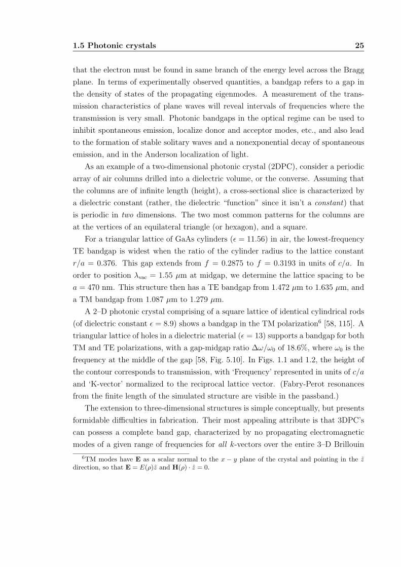
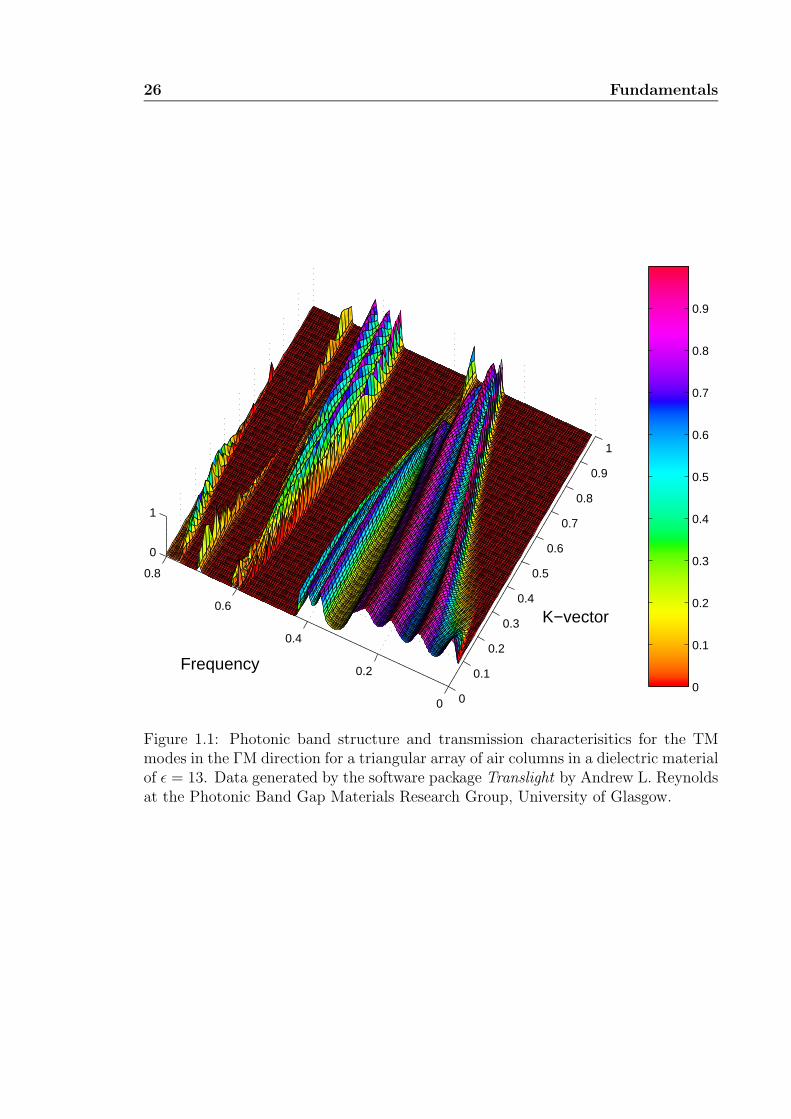
triangular lattice of holes in a dielectric material (ε = 13) supports a bandgap for both
TM and TE polarizations, with a gap-midgap ratio ∆ω/ω0 of 18.6%, where ω0 is the
frequency at the middle of the gap [58, Fig. 5.10]. In Figs. 1.1 and 1.2, the height of
the contour corresponds to transmission, with ‘Frequency’ represented in units of c/a
and ‘K-vector’ normalized to the reciprocal lattice vector. (Fabry-Perot resonances
from the finite length of the simulated structure are visible in the passband.)
The extension to three-dimensional structures is simple conceptually, but presents
formidable difficulties in fabrication. Their most appealing attribute is that 3DPC’s
can possess a complete band gap, characterized by no propagating electromagnetic
modes of a given range of frequencies for all k-vectors over the entire 3–D Brillouin
6TM modes have E as a scalar normal to the x − y plane of the crystal and pointing in the zdirection, so that E = E(ρ)z and H(ρ) · z = 0.
26 Fundamentals
0
0.1
0.2
0.3
0.4
0.5
0.6
0.7
0.8
0.9
0
0.1
0.2
0.3
0.4
0.5
0.6
0.7
0.8
0.9
1
0
0.2
0.4
0.6
0.8
0
1
K−vector
Frequency
Figure 1.1: Photonic band structure and transmission characterisitics for the TMmodes in the ΓM direction for a triangular array of air columns in a dielectric materialof ε = 13. Data generated by the software package Translight by Andrew L. Reynoldsat the Photonic Band Gap Materials Research Group, University of Glasgow.
1.5 Photonic crystals 27
0
0.1
0.2
0.3
0.4
0.5
0.6
0.7
0.8
0.9
0
0.2
0.4
0.6
0.8
1
0
0.1
0.2
0.3
0.4
0.5
0.6
0.7
0.8
0
1
K−vectorFrequency
Figure 1.2: Photonic band structure and transmission characterisitics for the TEmodes in the ΓM direction for a triangular array of air columns in a dielectric materialof ε = 13. Data generated by the software package Translight by Andrew L. Reynoldsat the Photonic Band Gap Materials Research Group, University of Glasgow.
28 Fundamentals
zone. A well-studied example is the face-centered cubic (diamond) lattice of air
spheres in GaAs (ε = 13), where the radius r is related to the lattice constant a by
r/a = 0.325. (The diameter of the air spheres is larger than the distance between
spheres, a√
3/2.)
Quasi-3–D structures such as photonic crystal slabs are similar to 2DPC’s in the
transverse profile of the dielectric function, but are of finite extent vertically. They
rely on index contrast with the surrounding material (e.g., air surrounding a slab of
GaAs) to confine modes to the slab vertically.
Many of the most interesting properties of photonic crystal structures arise when
the periodicity is intentionally interrupted, e.g., by filling in one of a periodic array
of air columns drilled into a GaAs slab. Borrowing once again from the terminology
of crystalline solids, this creates a “point defect” in the crystal. Point defects can
support localized high-Q modes [143], and line or surface defects can give rise to
propagating waveguide modes [108]. Much of the current understanding of photonic
crystal waveguides based on defects relies on numerical simulations, since the mode
structure of the individual defect modes is complicated. However, certain qualitative
features can be readily understood: as the translational symmetry of the structure
is destroyed, we can no longer use an in-plane wave vector to classify waveguide
modes, but mirror-reflection symmetry is still intact for in-plane propagation so that
TE and TM modes are still decoupled. If the eigenfrequency of the defect mode lies
in the photonic band gap, the defect-induced state must be evanescent, i.e., decay
exponentially away from the location of the defect in the plane of the structure.
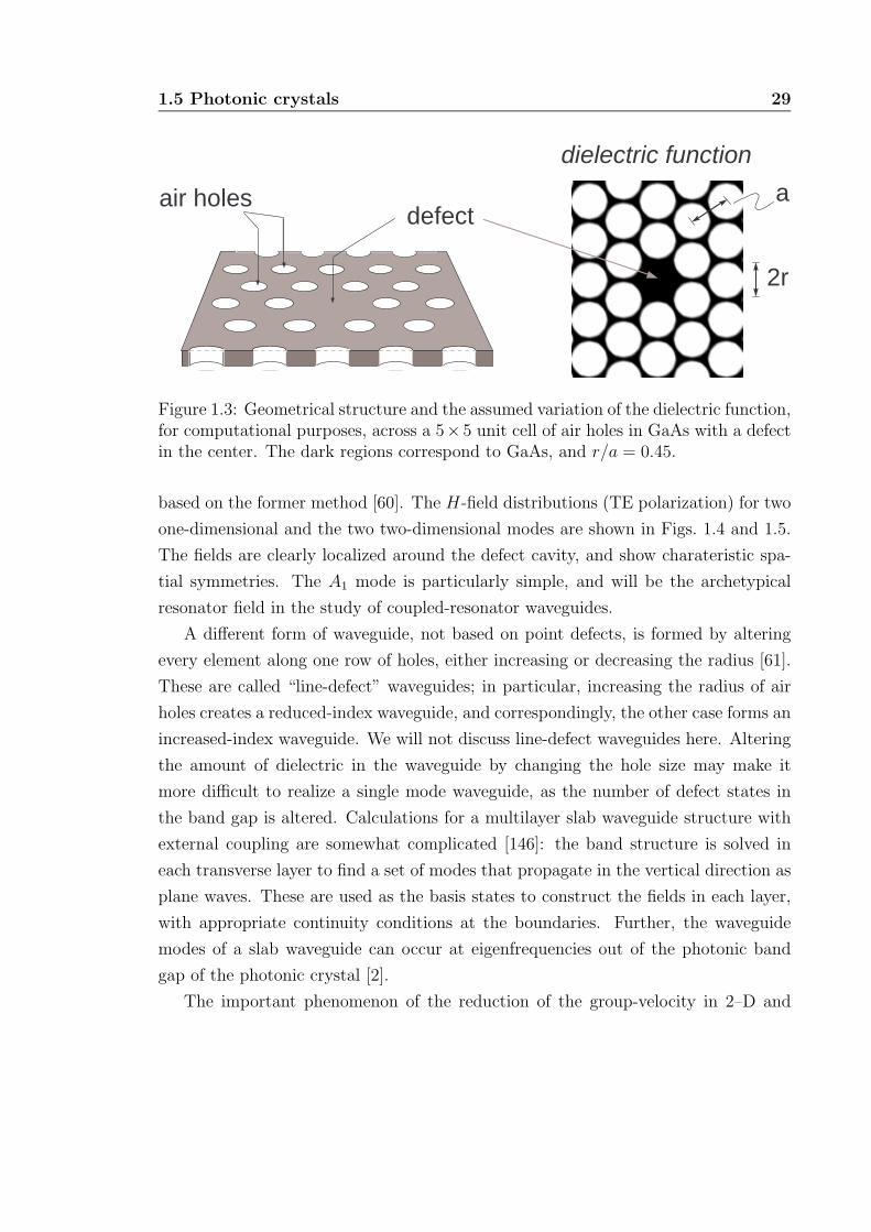
We will examine the defect modes of a triangular lattice of air holes in GaAs
(ε = 11.4) in some detail, because these modes will be used as the basic con-
stituents of coupled-resonator optical waveguides (CROWs). The transverse vari-
ation of the dielectric function over the computational unit cell is shown in Fig. 1.3.
The TE band structure of the uninterrupted periodic crystal shows a bandgap from
ωa/(2πc) = 0.307 to ωa/(2πc) = 0.495. Since the uninterrupted crystal exhibits
the C6v spatial symmetry, each localized eigenmode of the defect may be attributed
to one of its irreducible representations. There are four “one-dimensional” repre-
sentations (non-degenerate eigenvalues) and two “two-dimensional representations”
(doubly degenerate eigenvalues) [117, Ch. 6].
The defect mode field distributions may be calculated using either frequency-
domain or time-domain methods; here, we use a freely available software package
1.5 Photonic crystals 29
defectair holes a
2r
dielectric function
Figure 1.3: Geometrical structure and the assumed variation of the dielectric function,for computational purposes, across a 5× 5 unit cell of air holes in GaAs with a defectin the center. The dark regions correspond to GaAs, and r/a = 0.45.
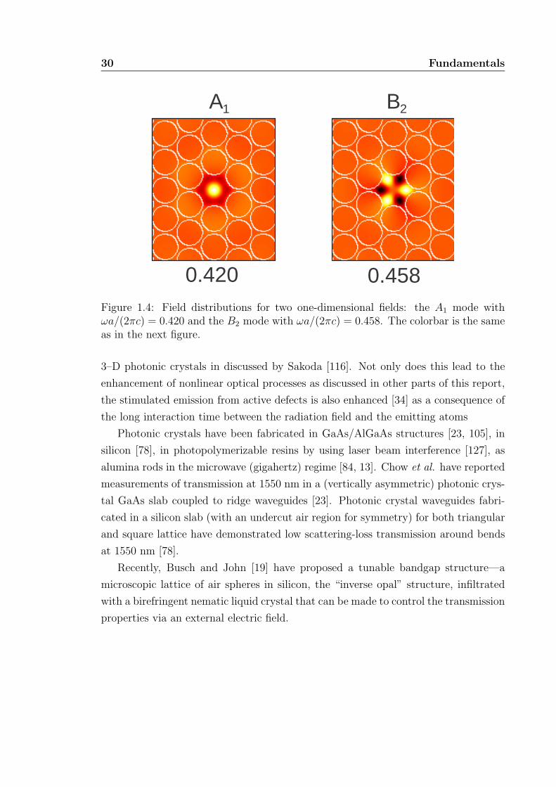
based on the former method [60]. The H-field distributions (TE polarization) for two
one-dimensional and the two two-dimensional modes are shown in Figs. 1.4 and 1.5.
The fields are clearly localized around the defect cavity, and show charateristic spa-
tial symmetries. The A1 mode is particularly simple, and will be the archetypical
resonator field in the study of coupled-resonator waveguides.
A different form of waveguide, not based on point defects, is formed by altering
every element along one row of holes, either increasing or decreasing the radius [61].
These are called “line-defect” waveguides; in particular, increasing the radius of air
holes creates a reduced-index waveguide, and correspondingly, the other case forms an
increased-index waveguide. We will not discuss line-defect waveguides here. Altering
the amount of dielectric in the waveguide by changing the hole size may make it
more difficult to realize a single mode waveguide, as the number of defect states in
the band gap is altered. Calculations for a multilayer slab waveguide structure with
external coupling are somewhat complicated [146]: the band structure is solved in
each transverse layer to find a set of modes that propagate in the vertical direction as
plane waves. These are used as the basis states to construct the fields in each layer,
with appropriate continuity conditions at the boundaries. Further, the waveguide
modes of a slab waveguide can occur at eigenfrequencies out of the photonic band
gap of the photonic crystal [2].
The important phenomenon of the reduction of the group-velocity in 2–D and
30 Fundamentals
0.420 0.458
A1 B2
Figure 1.4: Field distributions for two one-dimensional fields: the A1 mode withωa/(2πc) = 0.420 and the B2 mode with ωa/(2πc) = 0.458. The colorbar is the sameas in the next figure.
3–D photonic crystals in discussed by Sakoda [116]. Not only does this lead to the
enhancement of nonlinear optical processes as discussed in other parts of this report,
the stimulated emission from active defects is also enhanced [34] as a consequence of
the long interaction time between the radiation field and the emitting atoms
Photonic crystals have been fabricated in GaAs/AlGaAs structures [23, 105], in
silicon [78], in photopolymerizable resins by using laser beam interference [127], as
alumina rods in the microwave (gigahertz) regime [84, 13]. Chow et al. have reported
measurements of transmission at 1550 nm in a (vertically asymmetric) photonic crys-
tal GaAs slab coupled to ridge waveguides [23]. Photonic crystal waveguides fabri-
cated in a silicon slab (with an undercut air region for symmetry) for both triangular
and square lattice have demonstrated low scattering-loss transmission around bends
at 1550 nm [78].
Recently, Busch and John [19] have proposed a tunable bandgap structure—a
microscopic lattice of air spheres in silicon, the “inverse opal” structure, infiltrated
with a birefringent nematic liquid crystal that can be made to control the transmission
properties via an external electric field.
1.5 Photonic crystals 31
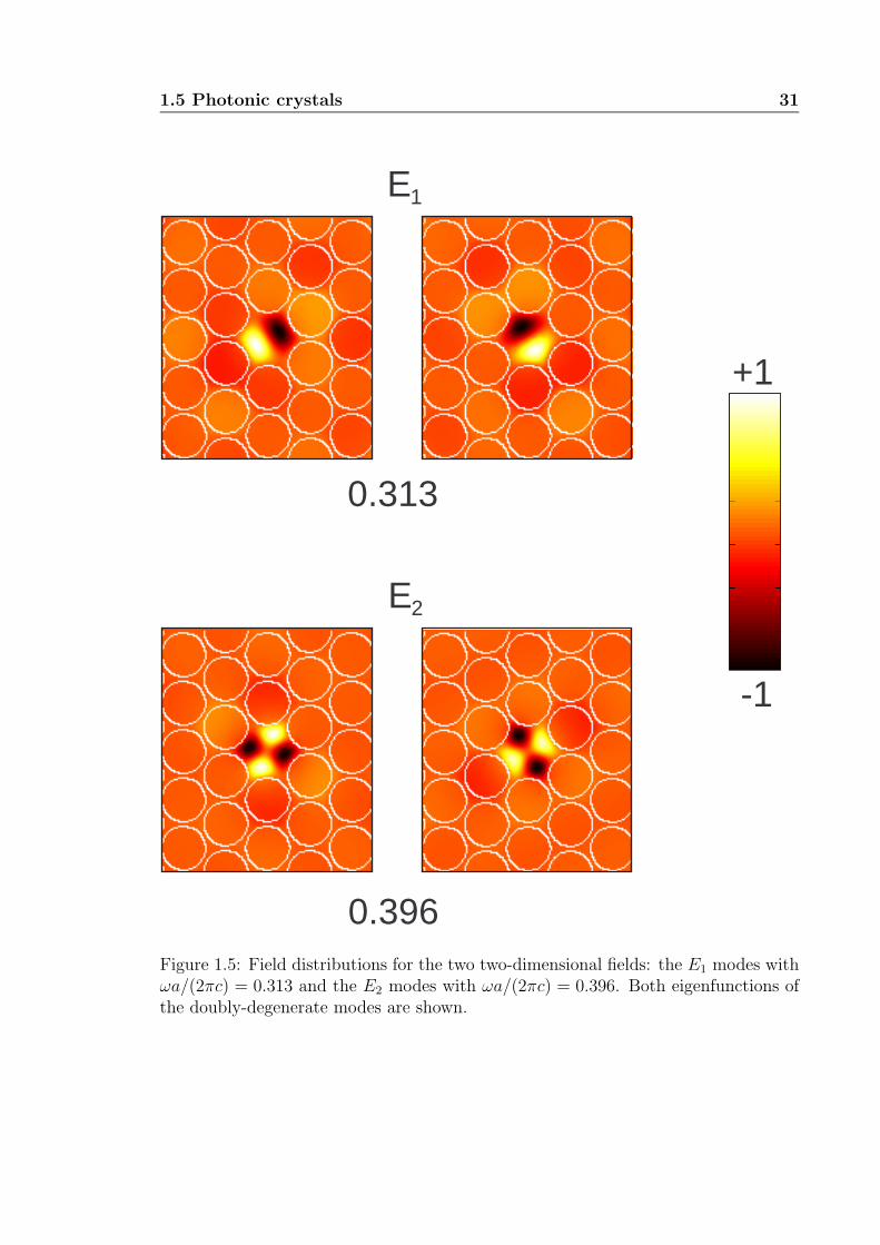
0.313
E1
0.396
E2
+1
-1
Figure 1.5: Field distributions for the two two-dimensional fields: the E1 modes withωa/(2πc) = 0.313 and the E2 modes with ωa/(2πc) = 0.396. Both eigenfunctions ofthe doubly-degenerate modes are shown.

32 Fundamentals
Chapter 2
Linear propagation in the tight-binding approximation
Operator techniques, functional techniques, renormalizationgroup methods, etc., are all available to take on any problem.
What is left open and is simply outside the scope of any of these methodsis the choice of “Equation (1)”, namely the starting point.
No solution technique, no matter how powerful, can derive a resultthat is not already implicit in the starting equation.
—John R. Klauder, Beyond Conventional Quantization, Cambridge (2000).
The development of integrated optoelectronic devices depends, in part, on the un-
derstanding of electromagnetic propagation in microstructure waveguides. Since this
electromagnetic radiation, for applications in communications, consists of pulses of
light, it’s important to explicitly account for temporal variations in the envelopes of
the fields. Mathematically, we discuss linear pulse propagation in one-dimensional
waveguides which do not exhibit spatial translation invariance symmetry, i.e., the
modes are not plane waves. Physical realizations of such structures include modu-
lated gratings in optical fibers or semiconductor materials, a linear array of defects
in a two-dimensional photonic crystal slab, and a chain of polystyrene microspheres.
2.1 Eigenmodes and “coupled mode theory”
Coupled-mode theory is a well-known formalism applicable to the problem of
propagation in an optical waveguide [154, Ch. 13]. It is a method of analysis of the
wave equation [154, 126, 57],
∇× [∇× E] +ε(r)
c2
∂2E
∂t2= − 1
c2
∂2
∂t2Ppert(r, t), (2.1)
33
34 Linear propagation in the tight-binding approximation
where Ppert(r, t) is a perturbation polarization that represents any deviation from the
unperturbed waveguide.
In the paraxial approximation, the total field in the waveguide is written as a
superposition of confined modes1; for TE modes propagating in a slab waveguide
along the z direction, the electric field,
Ey(r, t) =1
2
∑m
Am(z) E (m)y (x) ei(ωt−kmz) + c.c., (2.2)
is a sum of m discrete confined eigenmodes E (m)y (x), with propagation constants km
arising from an eigenvalue equation, modulated by an envelope Am(z).
Substituting the Ansatz Eq. (2.2) into Eq. (2.1) and assuming that derivatives of
second order of Am(z) can be ignored, we can obtain an ordinary differential equation
for Am(z) in terms of Ppert(r, t) and E (m)y (x) [154, Eq. (13.3-9)]. This approximation
in neglecting |d2Am/dz2| compared to km|dAm/dz| is known as the slowly varying
envelope approximation (SVEA).
This approach is useful in the description of wave propagation in gratings and other
periodic optical systems where the strength of the perturbation (relative to the free-
space equations) is weak. Not surprisingly, the same formalism has been applied in
solid state physics to the description of electrons in a weak periodic potential [129, 9].
The structure is viewed as a gas of nearly free conduction electrons, each of which
obeys the Schrodinger equation with a weak perturbation—the periodic potential of
the ions. When the periodic potential is exactly zero, the solutions to the Schrodinger
equation are plane waves [25], and these functions form a complete orthonormal
basis (over a finite interval) as in the well-known Fourier series expansion of periodic
functions2. The perturbative solution to the problem of a weak periodic potential is
then written as a superposition of these plane waves, with coefficients whose values
depend on the expansion of Ppert(r, t) in this basis.
Complementary to this weakly perturbative theory of coupled modes (which, con-
fusingly, is itself often called coupled-mode theory) is the tight-binding approxmation,
also known as the linear combination of atomic orbitals (LCAO) [62]. This approach
1Any coupling to radiation modes, which do not decay exponentially away from the waveguide,is ignored [154, pp. 492–494].
2Periodic functions can be thought of as the periodic extension of functions defined over a finiteinterval. For example, sin(x) over the entire real axis comprises replicas of the function f(x) =sin(x), |x| ≤ π, and which is identically zero for |x| > π.
2.1 Eigenmodes and “coupled mode theory” 35
describes electrons in a crystalline solid with a strong periodic potential due to the lat-
tice structure of localized atoms, characterized by a weak overlap between the atomic
wave functions [129, 9]. By analogy, the optical structures that can be described
using the tight-binding approximation are those that consist of isolated structural
elements (e.g., high-Q resonators such as defect modes in photonic crystals) weakly
coupled to one another. The propagating eigenmodes of the overall system are then
closely related to the eigenmodes of the individual elements, rather than the free-space
eigenmodes.
The wave function for a free electron wave is given by exp(−ik · r), where k is the
wave vector 3. This eigenmode is trivially of the Bloch form [129, pp. 156–160], since
free space can be thought of as periodic medium with an arbitrary small (or large)
period. In the tight-binding approximation, plane waves are not eigenmodes, but the
eigenmodes can still be written in the Bloch form. Lehmann and Ziesche point out
the differences between these two approaches quite early in their text [76, pp. 20–28],
as “the approximation starting from free electrons” and “the approximation starting
from free atoms.” In the words of Raimes [112, pp. 133],
One cannot say that either method is correct, but one or the other will give
better results in given circumstances and will be the more convenient as a basis
for more accurate calculations.
The energy of the wavefunction E is a function of the wave vector k. In terms
of the effective mass d2E/dk2 associated with electron levels, as the overlap between
the atomic energy levels decreases, the effective mass becomes very large, so that
electrons are indeed “tightly bound” to their atoms. For completely isolated atoms,
the group velocity dE/dk is zero, since the energies of all atoms are the same. But
once a band of energies is formed, an electron can move through the crystal, although
its group velocity may be small and its effective mass large.
Lehmann and Ziesche state in their text [76, pp. 36] that the tight-binding
expansion of the wave function of the crystal in terms of atomic orbital wavefuctions
φatn (r − R) is overcomplete since the latter form a complete system for each single
R. On the other hand, Ziman points out [161, pp. 95] that this set is incomplete
as “it lacks all the scattered-wave eigenstates of the Schrodinger equation in the
3In the terminology of solid-state physics, such functions when properly normalized are the eigen-functions of the Hartree equation describing a free-electron gas, and of the Hartree-Fock equationfor a monovalent metal, but with different eigenvalues in the two cases [112].
36 Linear propagation in the tight-binding approximation
continuum,” i.e., above the zero-energy level of the individual atomic wavefunction
potential (see Figs. 54 and 55 in [161].)
As pointed out, among other, by Jones [62, pp. 228–229], a significant criticism
of the tight-binding description, or perhaps of the independent electron approxi-
mation that is implicitly assumed in this description of electron levels in metals is
that it ignores positional correlations between electrons with antiparallel spins. In
the description of photons, this is not relevant as bands formed by different po-
larizations can be shown to be decoupled [150]. Further, every component of the
electromagnetic four-vector potential obeys the massless Klein-Gordon equation (in
the Lorentz gauge), without the need for anti-commutation relationships as are nec-
essary to describe spinor (Dirac) fields such as electrons [110]. In this way, we avoid
the overcounting of the states of a half-filled band in the case of electrons in a crystal
of widely separated monovalent atoms described by Jones.
The formalism is independent of the material in which the CROW geometry is
realized. Stefanou and Modinos have used the tight-binding method to analyze impu-
rity photonic bands in photonic insulators which can be described by a real negative
dielectric function ε(ω) [131]. The impurity cells are formed by introducing nonab-
sorbing dielectric spheres in a chain, and the resonances of the individual spheres
widen into a band of frequencies because of nearest-neighbor interactions. In this
chapter, we’ll focus on a particular case of the analysis in which the pulse envelope
propagates undistorted; these solutions may be thought of as the time-dependent
eigensolutions in the tight-binding approximation.
2.2 The tight-binding approximation
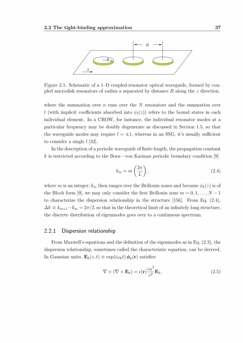
Assume that the resonators comprising the waveguide are identical and lie along
the z axis separated by a distance R as shown in Fig. 2.1. The total length of the
waveguide is taken to be L so that the number of resonators is N = L/R. A waveguide
mode—an eigenmode of a time-independent Hamiltonian—φk(z) with wavevector k
and propagation constant k = |k| is written as a linear combination of the individual
modes ψl(r) of the resonators that comprise the structure [9],
φk(r) =∑
n
exp(−inRk · z)∑
l
ψl(r − nRz) (2.3)
2.2 The tight-binding approximation 37
a
R
z
Figure 2.1: Schematic of a 1–D coupled-resonator optical waveguide, formed by cou-pled microdisk resonators of radius a separated by distance R along the z direction.
where the summation over n runs over the N resonators and the summation over
l (with implicit coefficients absorbed into ψl(z)) refers to the bound states in each
individual element. In a CROW, for instance, the individual resonator modes at a
particular frequency may be doubly degenerate as discussed in Section 1.5, so that
the waveguide modes may require l = ±1, whereas in an SSG, it’s usually sufficient
to consider a single l [32].
In the description of a periodic waveguide of finite length, the propagation constant
k is restricted according to the Born—von Karman periodic boundary condition [9]
km = m
(2π
L
), (2.4)
where m is an integer; km then ranges over the Brillouin zones and because φk(z) is of
the Bloch form [9], we may only consider the first Brillouin zone m = 0, 1, . . . , N − 1
to characterize the dispersion relationship in the structure [156]. From Eq. (2.4),
∆k ≡ km+1−km = 2π/L so that in the theoretical limit of an infinitely long structure,
the discrete distribution of eigenmodes goes over to a continuous spectrum.
2.2.1 Dispersion relationship
From Maxwell’s equations and the definition of the eigenmodes as in Eq. (2.3), the
dispersion relationship, sometimes called the characteristic equation, can be derived.
In Gaussian units, Ek(z, t) ≡ exp(iωkt) φk(r) satisfies
∇× (∇× Ek) = ε(r)ωk
2
c2Ek, (2.5)
38 Linear propagation in the tight-binding approximation
where ε(r) is the location-dependent dielectric coefficient of the waveguide and ωk is
the eigenfrequency of the waveguide mode. Replacing φk with ψl in Eq. (2.5) and ωk
with Ωl, the eigenfrequency of the l-th mode of a single resonator, we get a similar
equation that describes the eigenmode of a single resonator,
∇× (∇× ψl) = ε0(r)Ωl
2
c2ψl. (2.6)
To derive the dispersion relationship, we substitute Eq. (2.3) into Eq. (2.5), mul-
tiply both sides from the left by ψl(r)∗, and integrate over a unit cell, using the
normalization condition4
∫dr ε0(r) ψl(r)
∗ · ψm(r) = δlm, (2.7)
where ε0(r) is the dielectric coefficient of a single resonator in isolation, e.g., as shown
in Fig. 1.3.
After some algebra, the coefficient bl is found to satisfy a transcendental equa-
tion [150, Eq. (5)] which can be simplified under the conditions of weak (nearest-
neighbor) coupling and from symmetry considerations. Further, based on the sym-
metry of the individual resonator modes5 and considering the lowest-order individual
resonator modes, the dispersion relationship can be further simplified. Although the
single defect cavity modes are actually doubly degenerate, the two resultant CROW
bands have opposite polarity and can’t couple to each other; therefore, the dispersion
relation of each band has the same form.
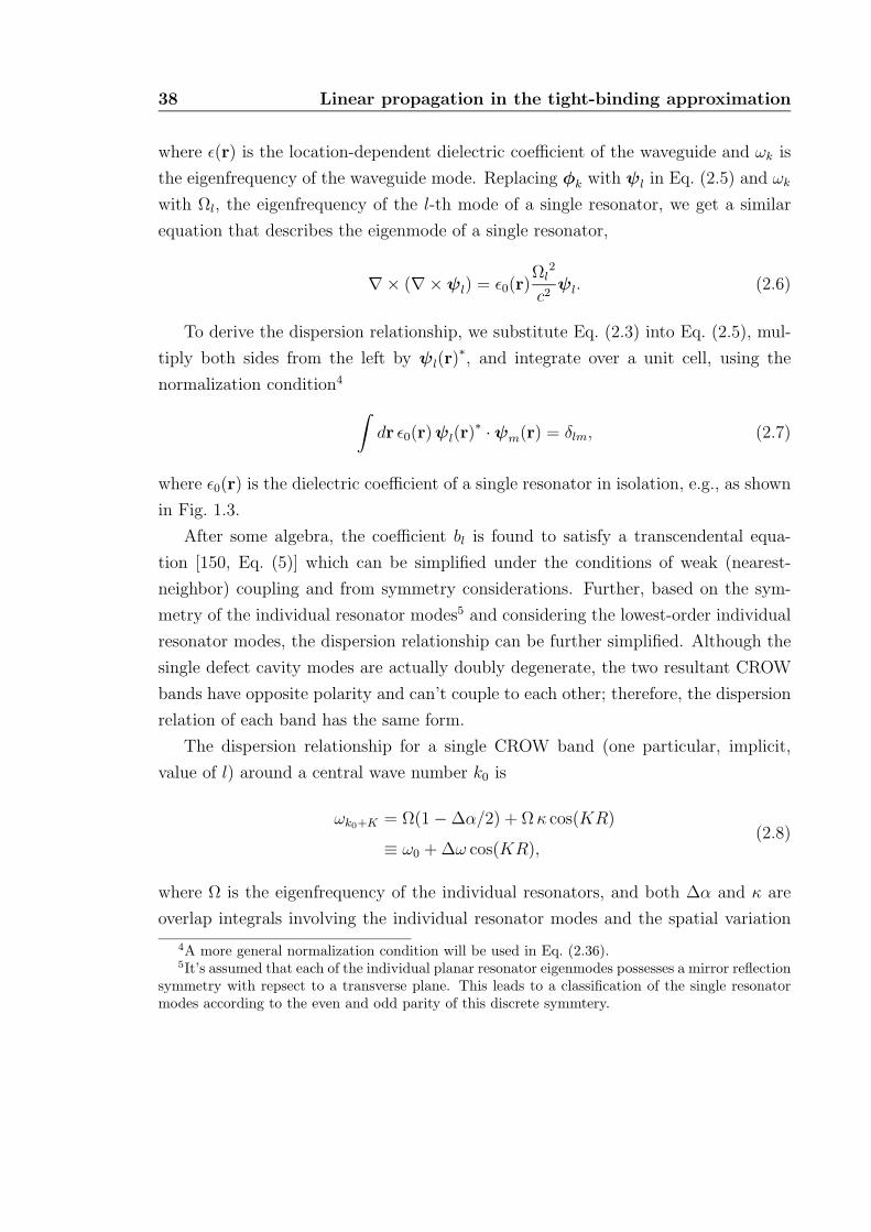
The dispersion relationship for a single CROW band (one particular, implicit,
value of l) around a central wave number k0 is
ωk0+K = Ω(1 − ∆α/2) + Ω κ cos(KR)
≡ ω0 + ∆ω cos(KR),(2.8)
where Ω is the eigenfrequency of the individual resonators, and both ∆α and κ are
overlap integrals involving the individual resonator modes and the spatial variation
4A more general normalization condition will be used in Eq. (2.36).5It’s assumed that each of the individual planar resonator eigenmodes possesses a mirror reflection
symmetry with repsect to a transverse plane. This leads to a classification of the single resonatormodes according to the even and odd parity of this discrete symmtery.
2.2 The tight-binding approximation 39
of the dielectric constant,
∆α =
∫d3r
[εwg(r − Rez) − εres(r − Rez)
]|ψl(r)|2
κ =
∫d3r
[εres(r − Rez) − εwg(r − Rez)
]ψl(r) · ψl(r − Rez),
(2.9)
where εres is the dielectric constant of the individual resonators, and εwg is the dieletric
constant of the waveguide. This is similar to an equivalent derivation in the electronic
levels of crystalline solids in the tight-binding approximation [129, pp. 200–212].
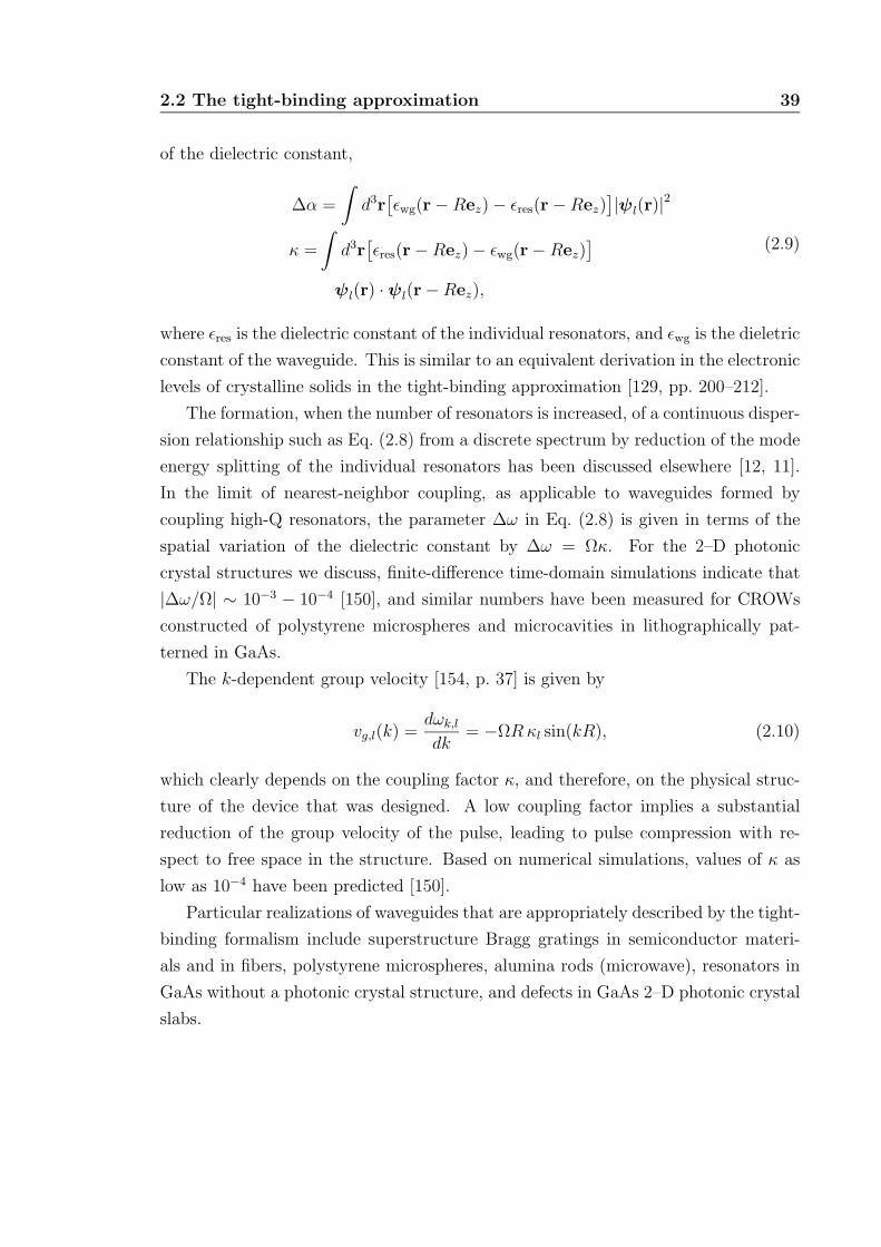
The formation, when the number of resonators is increased, of a continuous disper-
sion relationship such as Eq. (2.8) from a discrete spectrum by reduction of the mode
energy splitting of the individual resonators has been discussed elsewhere [12, 11].
In the limit of nearest-neighbor coupling, as applicable to waveguides formed by
coupling high-Q resonators, the parameter ∆ω in Eq. (2.8) is given in terms of the
spatial variation of the dielectric constant by ∆ω = Ωκ. For the 2–D photonic
crystal structures we discuss, finite-difference time-domain simulations indicate that
|∆ω/Ω| ∼ 10−3 − 10−4 [150], and similar numbers have been measured for CROWs
constructed of polystyrene microspheres and microcavities in lithographically pat-
terned in GaAs.
The k-dependent group velocity [154, p. 37] is given by
vg,l(k) =dωk,l
dk= −ΩR κl sin(kR), (2.10)
which clearly depends on the coupling factor κ, and therefore, on the physical struc-
ture of the device that was designed. A low coupling factor implies a substantial
reduction of the group velocity of the pulse, leading to pulse compression with re-
spect to free space in the structure. Based on numerical simulations, values of κ as
low as 10−4 have been predicted [150].
Particular realizations of waveguides that are appropriately described by the tight-
binding formalism include superstructure Bragg gratings in semiconductor materi-
als and in fibers, polystyrene microspheres, alumina rods (microwave), resonators in
GaAs without a photonic crystal structure, and defects in GaAs 2–D photonic crystal
slabs.
40 Linear propagation in the tight-binding approximation
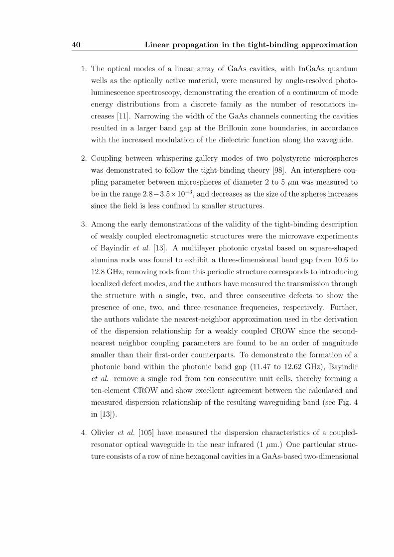
1. The optical modes of a linear array of GaAs cavities, with InGaAs quantum
wells as the optically active material, were measured by angle-resolved photo-
luminescence spectroscopy, demonstrating the creation of a continuum of mode
energy distributions from a discrete family as the number of resonators in-
creases [11]. Narrowing the width of the GaAs channels connecting the cavities
resulted in a larger band gap at the Brillouin zone boundaries, in accordance
with the increased modulation of the dielectric function along the waveguide.
2. Coupling between whispering-gallery modes of two polystyrene microspheres
was demonstrated to follow the tight-binding theory [98]. An intersphere cou-
pling parameter between microspheres of diameter 2 to 5 µm was measured to
be in the range 2.8−3.5×10⁻³, and decreases as the size of the spheres increases
since the field is less confined in smaller structures.
3. Among the early demonstrations of the validity of the tight-binding description
of weakly coupled electromagnetic structures were the microwave experiments
of Bayindir et al. [13]. A multilayer photonic crystal based on square-shaped
alumina rods was found to exhibit a three-dimensional band gap from 10.6 to
12.8 GHz; removing rods from this periodic structure corresponds to introducing
localized defect modes, and the authors have measured the transmission through
the structure with a single, two, and three consecutive defects to show the
presence of one, two, and three resonance frequencies, respectively. Further,
the authors validate the nearest-neighbor approximation used in the derivation
of the dispersion relationship for a weakly coupled CROW since the second-
nearest neighbor coupling parameters are found to be an order of magnitude
smaller than their first-order counterparts. To demonstrate the formation of a
photonic band within the photonic band gap (11.47 to 12.62 GHz), Bayindir
et al. remove a single rod from ten consecutive unit cells, thereby forming a
ten-element CROW and show excellent agreement between the calculated and
measured dispersion relationship of the resulting waveguiding band (see Fig. 4
in [13]).
4. Olivier et al. [105] have measured the dispersion characteristics of a coupled-
resonator optical waveguide in the near infrared (1 µm.) One particular struc-
ture consists of a row of nine hexagonal cavities in a GaAs-based two-dimensional
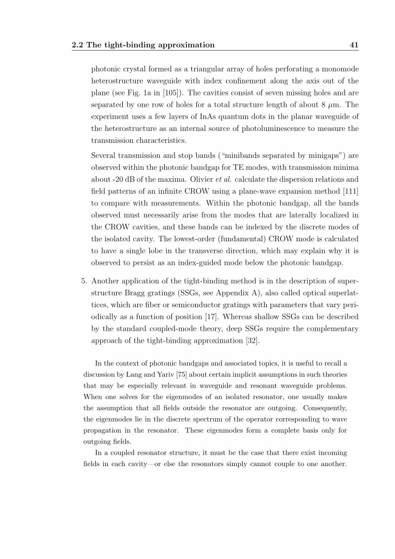
2.2 The tight-binding approximation 41
photonic crystal formed as a triangular array of holes perforating a monomode
heterostructure waveguide with index confinement along the axis out of the
plane (see Fig. 1a in [105]). The cavities consist of seven missing holes and are
separated by one row of holes for a total structure length of about 8 µm. The
experiment uses a few layers of InAs quantum dots in the planar waveguide of
the heterostructure as an internal source of photoluminescence to measure the
transmission characteristics.
Several transmission and stop bands (“minibands separated by minigaps”) are
observed within the photonic bandgap for TE modes, with transmission minima
about -20 dB of the maxima. Olivier et al. calculate the dispersion relations and
field patterns of an infinite CROW using a plane-wave expansion method [111]
to compare with measurements. Within the photonic bandgap, all the bands
observed must necessarily arise from the modes that are laterally localized in
the CROW cavities, and these bands can be indexed by the discrete modes of
the isolated cavity. The lowest-order (fundamental) CROW mode is calculated
to have a single lobe in the transverse direction, which may explain why it is
observed to persist as an index-guided mode below the photonic bandgap.
5. Another application of the tight-binding method is in the description of super-
structure Bragg gratings (SSGs, see Appendix A), also called optical superlat-
tices, which are fiber or semiconductor gratings with parameters that vary peri-
odically as a function of position [17]. Whereas shallow SSGs can be described
by the standard coupled-mode theory, deep SSGs require the complementary
approach of the tight-binding approximation [32].
In the context of photonic bandgaps and associated topics, it is useful to recall a
discussion by Lang and Yariv [75] about certain implicit assumptions in such theories
that may be especially relevant in waveguide and resonant waveguide problems.
When one solves for the eigenmodes of an isolated resonator, one usually makes
the assumption that all fields outside the resonator are outgoing. Consequently,
the eigenmodes lie in the discrete spectrum of the operator corresponding to wave
propagation in the resonator. These eigenmodes form a complete basis only for
outgoing fields.
In a coupled resonator structure, it must be the case that there exist incoming
fields in each cavity—or else the resonators simply cannot couple to one another.
42 Linear propagation in the tight-binding approximation
These fields cannot be described by the modes of an individual resonator, to which
must be added the modes corresponding to the continuous spectrum, corresponding
to fields incident on the cavity from the outside. If we drop this continuous part of
the spectrum, we conceptually introduce “black hole” modes, which in rate equations
act as sinks for energy from the discrete modes but never as sources to the discrete
modes. There is no mechanism for the scattering of energy back from the black hole
modes to the modes we do consider. As a result, calculations of threshold gains from
such a theory will be overestimated, and the fraction of overestimation depends on
the relative fraction of the coupled-cavity modes that is described by the black hole
modes.
For weakly coupled resonators, as in a CROW waveguide, this may be small, but
when the coupling becomes significant, as in a CROW laser, it may be significant.
Although the CROW laser is not discussed here, we point out that Lang and Yariv
have formulated local-field rate equations in terms of the amplitudes of traveling
waves at fixed points inside the composite cavity, rather than the amplitude of an
individual cavity mode [74, 75]. The central approximation made is that the optical
field adiabatically follows the characteristics of the resonator.
2.3 Pulse propagation
Based on our earlier analysis of the individual resonator modes, and the waveguide
modes, we can now analyze how a pulse propagates in a CROW. At a fixed time, taken
for simplicity to be t = 0, the field in the waveguide is given by a superposition of
eigenmodes,
E(r, t = 0) =
∫dk
2πck φk(r), (2.11)
where φk(r) are the eigenmodes at wavevector (propagation constant) k as given by
Eq. (2.3) and ck are certain ‘weights’ to be determined from the boundary condition6.
For a structure of finite length, not all k’s are allowed, according to Eq. (2.4),
and the integral over k in Eq. (2.11) should be replaced by a sum over the allowed
k. Alternatively, we can redefine φk(z) for a 1D structure of finite length along the
6The geometry of the problem dictates that we adopt the methodology of Section 1.2 rather thanof Section 1.1.
2.3 Pulse propagation 43
z-axis as
φk(r) =
[|∆k|
∞∑m=−∞
δ(k − m∆k)
]∑n
exp(−inkR)∑
l
ψl(r − nRez) (2.12)
to preserve the form of Eq. (2.11). The factor |∆k| inside the square brackets in
Eq. (2.12) follows from the usual definition of the Riemann-Stieltjes integral [8]: for
a long waveguide, as L → ∞ and ∆k → 0, the field E(z, t = 0) retains the same
form as given directly by Eq. (2.11) with φk(z) defined by Eq. (2.3), i.e., without the
impulse train (in square brackets) in Eq. (2.12).
Since the system is linear and time invariant, the field at time t is given by
E(z, t) =
∫dk
2πeiω(k)tckφk(z). (2.13)
Since the dispersion relationships of the waveguide modes are approximately linear in
the middle of the band gap (the group velocity goes to zero at the band edges) [156,
32], we can write the dispersion relationship around the central propagation constant
of the pulse k0 as
ω(k0 + K) = ω(k0) +dω
dk
∣∣∣∣k=k0
K + . . . ≈ ω0 + vgK, (2.14)
where vg is the group velocity of the pulse. Then,
E(r, t) = eiω0t
∫dK
2πeivgtKck0+K φk0+K(r). (2.15)
The boundary conditions specify a pulse shape at the z = 0 edge of the waveguide
and centered at the optical frequency ω0,
E(r = 0, t) = eiω0tE(z = 0, t)u, (2.16)
where u is a unit-magnitude vector that describes the vectorial nature of the field at
r = 0. The vectorial behavior of φk0+K(0) must follow u.
We’ll work with the scalar functions φk0+K(z) and ψl(z) in the remainder of this
section, and in the following section. From the equality of Eq. (2.15) evaluated at
44 Linear propagation in the tight-binding approximation
z = 0 and Eq. (2.16), it follows that
ck0+K =1
φk0+K(0)
∫d(|vg|t′) E(z = 0, t′)e−ivgt′K . (2.17)
Combining Eq. (2.15) and Eq. (2.17),
E(z, t) = eiω0t
∫d(|vg|t′) E(z = 0, t′)
∫dK
2π
φk0+K(z)
φk0+K(0)eivg(t−t′)K . (2.18)
In free space, which can be thought of as a “linear space-invariant system,” the
eigenfunctions are φk(z) = exp(−ikz), instead of Eq. (2.3). Substituting this into
Eq. (2.18), we get
E(z, t) = eiω0t
∫d(|vg|t′) E(z = 0, t′)
∫dK
2πe−i(k0+K)z eivg(t−t′)K
= ei(ω0t−k0z)E
(z = 0, t − z
vg
). (2.19)
This is the well-known result (similar to Eq. (1.6) and Jackson [57, pp. 322–326]) that
a pulse propagates unchanged in shape in a weakly dispersive medium, apart from
an overall phase factor, and that the velocity of propagation is given by the group
velocity of the pulse vg defined from the dispersion relationship as in Eq. (2.14).
In Chapter 3, we’ll extend the above description to account for propagation in
waveguides that can amplify or attenuate the pulse, or otherwise transfer power be-
tween the various waveguide modes that comprise the pulse. The goal is to identify, if
possible, a component of that field description that is analogous to, e.g., the envelope
of a conventional waveguide mode, exp[i(ωt− kz)]. By identifying the envelope com-
ponent of the full field description, we may obtain equations that describe the change
in the envelope alone, and do not involve the variables describing the non-envelope
part of the field. It’s usually the case that the envelope usually varies on a longer
spatial scale than the remainder of the field.
CROWs and SSGs in the tight-binding approximation do not have plane-wave
eigenmodes of the form exp[i(ωt − kz)]. For a structure whose eigenmodes are given
by Eq. (2.3) or Eq. (2.12) with ψ(z) rapidly decaying in magnitude for distances
on the order of R, we can carry out further simplifications to the field expression
Eq. (2.18).
2.3 Pulse propagation 45
The individual resonator eigenmodes are normalized as ψl(0) = 1 and are highly
localized around z = 0 so that |ψl(nR)| 1 for all n = 0. We assume that these
eigenmodes are symmetric, so that ψl(−z) = ψl(z). Then,
φk0+K(0) =∑
n
e−i(k0+K)nR∑
l
ψ(−nR)
= 1 +∑
l
ψl(R) 2 cos[(k0 + K)R] + . . . (2.20)
ignoring terms on the order of∑
l ψ(2R) or smaller. Consequently, we can write
[φk0+K(0)]−1 ≈ 1 −∑
l
ψl(R) 2 cos[(k0 + K)R], (2.21)
which can be used in Eq. (2.18).
The leading order contribution to E(z, t) is given by including the first term of
Eq. (2.21),
E(z, t) = eiω0t∑
n
e−ik0nR∑
l
ψl(z − nR)
∫d(|vg|t′) E(z = 0, t′)
×∫
dK
2π
[|∆K|
∑m
δ(K − m∆K)
]eiTK , (2.22)
where T ≡ vg(t − nR/vg − t′), and the index m of the infinite summation can be
translated as desired. The expression on the second line of Eq. (2.22) is the inverse
Fourier transform (evaluated at T ) of an impulse train in the K domain, which
evaluates to an impulse train in the T domain [107],
|∆K|∞∑
m=−∞δ(K − m∆K)
∞∑m=−∞
δ(T − m∆T ), (2.23)
where ∆T = 2π/∆K = L. Carrying out the integrals over t′ for each m,
E(z, t) = eiω0t∑
n
e−ik0nR∑
l
ψl(z − nR)∑m
E
(z = 0, t − nR + mL
vg
). (2.24)
This expression is the tight-binding approximation analog of Eq. (2.19). The vectorial
extension is written in Eq. (2.32).
46 Linear propagation in the tight-binding approximation
It will be shown in Section 2.5 that Eq. (2.24) is of the Bloch form, i.e., E(z, t)
can be written as the product of a plane wave exp[i(ωt − kz)] and a function u(z, t)
with the periodicity of the “lattice” that defines the CROW. It’s important to note,
however, that this does not imply that plane waves of the form exp[i(ωt − kz)] are
eigenfunctions of the CROW as the function u(z, t) is not necessarily slowly varying
(and in fact, varies as “rapidly” as exp[−ikz] does).
The contribution of the first-order corrections to Eq. (2.24) based on Eq. (2.21)
can be evaluated in the same way,
∆E(z, t) = −∑
l′ψl′(R)eiω0t
∑n
e−ik0(n−1)R∑
l
ψl(z − nR) ×∑m
E
(z = 0, t − (n − 1)R + mL
vg
)+∑
n
e−ik0(n+1)R ×
∑l
ψl(z − nR)∑m
E
(z = 0, t − (n + 1)R + mL
vg
). (2.25)
Fig. 2.2 shows an annotated frame from an MPEG animation of Gaussian pulse
propagation in a structure described by the tight-binding approximation to the leading
order, using the approximations that the structure is of infinite length and that it’s
sufficient to consider a single l in Eq. (2.24).
Although Eq. (2.15) is a good approximation to the dispersion relationship in a
CROW [156, 150], it may be necessary for wideband pulses to consider higher-order
terms in Eq. (2.15). The resulting Eq. (2.17) is then obtained from the solution of a
Fredholm integral equation, and Eqs. (2.18) and (2.24) will in general involve envelope
distortion (as for free space propagation [154]).
2.4 Frequency, space, and time sampling
As we’ve already noted, the allowed k vectors are quantized in a structure of
finite length, and using Eq. (2.14), the allowed ω = ω0 + Ω values are quantized. To
prevent aliasing [107], the temporal interval between two samples 2π/∆Ω must be
greater than twice the temporal extent of the pulse envelope T , where ∆Ω = vg∆K
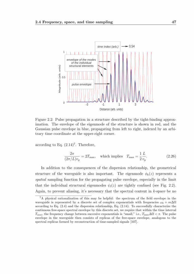
2.4 Frequency, space, and time sampling 47
-3 -1 1 30
0.5
1
0.54
Distance (arb. units)
Ma
gn
itu
de
(a
rb.
un
its)
time index (arb.)
envelope of the modesof the individual
structural elements
pulse envelope
Figure 2.2: Pulse propagation in a structure described by the tight-binding approx-imation. The envelope of the eigenmode of the structure is shown in red, and theGaussian pulse envelope in blue, propagating from left to right, indexed by an arbi-trary time coordinate at the upper-right corner.
according to Eq. (2.14)7. Therefore,
2π
(2π/L)vg
= 2Tmax, which implies Tmax =1
2
L
vg
. (2.26)
In addition to the consequences of the dispersion relationship, the geometrical
structure of the waveguide is also important. The eigenmode φk(z) represents a
spatial sampling function for the propagating pulse envelope, especially in the limit
that the individual structural eigenmodes ψl(z) are tightly confined (see Fig. 2.2).
Again, to prevent aliasing, it’s necessary that the spectral content in k-space be no
7A physical rationalization of this may be helpful: the spectrum of the field envelope in thewaveguide is represented by a discrete set of complex exponentials with frequencies ω0 + m∆Ωaccording to Eq. (2.4) and the dispersion relationship, Eq. (2.14). To successfully characterize thecontinuous free-space spectral envelope by this discrete set, we require that within the time intervalTmax, the frequency change between succesive exponentials is “small,” i.e., Tmax∆Ω < π. The pulseenvelope in the waveguide then consists of replicas of the free-space envelope, analogous to thespectral replicas formed by reconstruction of time-sampled signals [107].
48 Linear propagation in the tight-binding approximation
greater than Kmax,
2π
R= 2Kmax which implies Kmax =
1
2
(2π
R
). (2.27)
But the free-space pulse envelope is invariant in the frame z−vgt, and this maximum
K-space extent translates into a minimum pulse width Tmin,8
1
2vgTmin = R which implies Tmin =
2R
vg
. (2.28)
In a structure of finite length described by the tight-binding approximation, therefore,
there exists both a maximum and a minimum allowed pulse duration; the former arises
because of the finite length of the structure, and the latter because of the sampling
train-like eigenmodes of the waveguide.
Eq. (2.28) limits the bandwidth (where most of the energy of the pulse is concen-
trated) in the Fourier K-space associated with the propagation distance z, and since
the pulse is propagating with group velocity vg, also in the Fourier Ω-space associated
with the temporal coordinate t. The dimension of the space of finite-energy signals
(pulse envelopes) that are identically zero outside the time interval [−T0/2, T0/2] and
have most of their energy concentrated in the bandwidth [−Ω0/2, Ω0/2] is approxi-
mately D = Ω0T0 + 1 [147],
D =
(1
Rvg
)(1
2
L
vg
)+ 1 =
N
2+ 1, (2.29)
where N = L/R is the number of individual structural elements in the waveguide.
These pulse envelopes can be represented in the mean-square sense by a superposition
of the prolate spheroidal wave functions within the interval [−Tmax/2, Tmax/2].
2.4.1 K-space representation of Eq. (2.24)
It’s often convenient in certain problems (e.g., four-wave mixing processes [91])
to have a description of the spatial Fourier transform of Eq. (2.24) in terms of plane
8As a guideline, it’s useful to recall that the Fourier transform of a rectangular pulse between±vgT in the vgt frame is a sinc function with first nulls at ±π/(vgT ) in K-space [107].
2.5 Linear pulse propagation: Bloch waves 49
waves,
E(K, t) ≡∫
E(z, t)e−iKzdz
= eiω0t∑
n
e−i(k0+K)nR∑m
E
[z = 0, t − nR + mL
vg
]∑l
ψl(K), (2.30)
where ψl(K) =∫
ψl(z) exp(−iKz) dz is the spatial Fourier transform of ψl(z).
Eqs. (2.24) and (2.30) describe the propagation of a pulse in a medium described
by the tight-binding approximation. They can be used, for example, to describe the
index grating formed by the interference pattern of two counterpropagating pulses
(at the same optical frequency for simplicity),
δn(z) ∝∫
dK1
2π
∫dK2
2πδn(K1, K2) ei(K1−K2)zE(K1, t)E(K2, t)
∗, (2.31)
where δn(K1, K2) is the coupling coefficient between two plane waves defined by K1
and K2 and depends on the material properties, the orientation of the medium and
the polarization of the waves [123].
We’ve formed equations describing the evolution of optical pulses in
the tight-binding approximation, which is of increasing importance in
the description of a variety of recently developed structures such as cou-
pled resonator optical waveguides in photonic crystals and superstructure
Bragg gratings in both semicondutors and in optical fiber. These equa-
tions form a useful starting point for the analysis of linear and nonlinear
pulsed phenomena in such structures.
2.5 Linear pulse propagation: Bloch waves
In this section, we’ll modify Eq. (2.24) in three ways. Firstly, we limit our attention
to the limiting case of an infinitely long waveguide and drop the summation over m.
Secondly, we’ll account for the vectorial nature of the individual resonator modes ψ(r)
but we’ll continue to look at pulse propagation along the z-axis. For simplicity, we’ll
also omit the summation over the multiple modes of individual resonators, indexed
50 Linear propagation in the tight-binding approximation
by l: their re-introduction is straightforward. The electric field distribution Ek(r, t)
describing a pulse at the frequency ω and wave vector K is
Ek(r, t) = eiω0t∑
n
e−iknR ψ(r − nRez)E[z = 0, t − nR
v
](2.32)
where ψ(r) is the individual resonator eigenmode, E(z = 0, t) is the input pulse
envelope9 and v is the group velocity at K = |K|.For an infinitely long CROW, where the summation over n in Eq. (2.32) can be
relabeled to n ± 1, EK(r, t) satisfies the (3+1)D Bloch theorem [154, 9],
Ek(r + Rez, t + R/v) = eiωR/ve−ikREk(r, t). (2.33)
Consequently, the waveguide field distribution can be written in the Bloch form,
Ek(r, t) = eiωte−ik(ω)z uk(ω)(r, t), (2.34)
where uk(ω)(r, t) is a vector-valued function with the periodicity of the CROW “lat-
tice” and can be written out explicitly as
uk(ω)(r, t) =∑
n
eik(z−nR) ψ(r − nRez) E[z = 0, t − nR
v
]. (2.35)
The notation emphasises that the propagation constant k and the Bloch wave func-
tion depend on the frequency ω (we’ll sometimes write kω in place of k(ω) so that
the mathematical structure of certain equations is not obscured). Nevertheless, our
writing the electromagnetic field distribution in the Bloch form, Eq. (2.34), is mainly
for notational convenience in Section 3.3.
The Bloch wave function is normalized according to the following inner product
definition between the vector space of the Bloch wave function and its dual space,
∫dt
T
∫dr ε(r)
[uk(ω)(r, t)
]∗ · uk(ω)(r, t) = 1, (2.36)
9The terminology “input pulse envelope” shouldn’t be taken too literally since the structures weconsider are infintely long: it merely means that we focus on the field evolution along a section ofan infinite waveguide, and the “input” refers to the field distribution at one edge of this structure,i.e., a boundary condition, as discussed in Chapter 2. The precise mathematical meaning of thisassumption is rather technical and is discussed at the end of Appendix C.
2.5 Linear pulse propagation: Bloch waves 51
where the spatial integration extends over a unit cell and the temporal integration
over the extent of the pulse envelope, with a characteristic time constant T . This
ensures that Eq. (2.36) still represents an electromagnetic energy conservation rela-
tionship [57], and can be interpreted as yielding a time-averaged energy stored in a
unit cell volume [113, pp. 404–405]. We’ll abbreviate the notation in Eq. (2.36) to an
integration over the 4-vector r.
Based on Maxwell’s equation, the waveguide field distribution satisfies the follow-
ing equation: [154, 57]
∇× [∇× E] +ε(r)
c2
∂2E
∂t2= 0. (2.37)
Substituting Eq. (2.34) for E(r, t), we can write Eq. (2.37) as an eigenvalue prob-
lem [96] for the Bloch wavefunction uk(ω)(r, t),
Hkuk(ω) ≡ −kω2ez × [ez × uk(ω)] + ∇× [∇× uk(ω)]
− ikω
[ez× [∇× uk(ω)] + ∇× [ez × uk(ω)]
]+
ε(r)
c2
[∂2uk(ω)
∂t2+ i 2ω
∂uk(ω)
∂t
]
=ω2
c2ε(r)uk(ω).
(2.38)
It can be shown that the operator H is Hermitian (see Appendix C for an outline
of the proof.) As a consequence of the dispersion relationship in the waveguide [57],
the eigenvalue ω2/c2 is parametrized by K and we can use the Hellman-Feynman10
theorem [52, 37, 25, 119],
d(w/c)2
dk=
∫d4r
[uk(ω)
]∗ · [− 2kωez × [ezuk(ω)]
− iez × [∇× uk(ω)] − i∇× [ez × uk(ω)]]
+ i2
c2
dω
dk
∫d4r ε(r)
[uk(ω)
]∗ · ∂uk(ω)
∂t.
(2.39)
Recognizing that dω/dk defines the group velocity v [154], Eq. (2.39) can be re-
10R. P. Feynman was an undergraduate at MIT at the time of writing this paper (1939).
52 Linear propagation in the tight-binding approximation
written as
v
[2ω
c2− i
2
c2
∫d4r ε(r)
[uk(ω)
]∗ · ∂uk(ω)
∂t
]=
∫d4r
[uk(ω)
]∗ · [− 2kωez × [ezuk(ω)]
− iez × [∇× uk(ω)] − i∇× [ez × uk(ω)]]. (2.40)
This equation will be of considerable use in Chapter 3, where we discuss nonlinear
optical phenomena in CROWs.
2.6 Using the full dispersion relationship
From Eq. (2.16), the coefficients ck0+K are derived from
E(z = 0, t) =
∫ π/R
−π/R
dK
2πei∆ωt cos(KR)ck0+K φk0+K(0). (2.41)
This is easily inverted in the limit of a linear dispersion relationship in place of
Eq. (2.8)—the integral operator reduces to the well-known Fourier transform, and this
is the analysis we have discussed earlier. In considering higher-order dispersion terms
in the Taylor series expansion of the dispersion relationship, the integral equation,
Eq. (2.41), can’t in general be inverted to obtain the c’s in closed form. This is
clearly evident when, for example, the exponent involves terms of quadratic or higher
polynomial powers of K. Therefore, rather than work with the successive terms in a
Taylor-series expansion of the dispersion relationship, we’ll work with the full form
of Eq. (2.8).
Note that the dispersion relationship is symmetric about K = 0. We’ll assume that
E(z = 0, t) is a symmetric envelope. Consequently, ck0+K φk0+K(0) = ck0−K φk0−K(0)
for all K within the first Brillouin zone. This is not a critical assumption, and relates
to the choice of cosines rather than sines a subsequent step [Eq. (2.44)].
We introduce changes of variables to highlight the mathematical structure of
2.6 Using the full dispersion relationship 53
Eq. (2.41),
ϕ ≡ KR,
x ≡ ∆ωt,
h(φ) ≡ ck0+K φk0+K(0),
f(x) ≡ 2R E(z = 0, x/∆ω),
(2.42)
so that Eq. (2.41) becomes
πf(x) =
∫ π
−π
dϕ eix cos ϕh(ϕ), (2.43)
where f(x) is a known function, in terms of which we want to find h(ϕ). For the
majority of cases of practical interest, we can instead find the coefficients in the
expansion of h(ϕ) as a Fourier cosine series,
h(ϕ) =∞∑
n=0
cn cos(nϕ). (2.44)
Using the identity [154, Eq. (9.4-5)],
eix cos ϕ =∞∑
m=0
bm Jm(x) cos(mϕ),
where bm =
1, m = 0
2im, m ≥ 1
(2.45)
and the orthogonality of the cosines over the interval (−π, π), we can simplify Eq. (2.43)
to
f(x) =∞∑
n=0
(bncn) Jn(x) ≡∞∑
n=0
anJn(x). (2.46)
Therefore, if we can expand f(x) [which describes the envelope at the z = 0 cross
section—see Eq. (2.42)] in a Neumann series [145, Chap. IX], we can find the co-
efficients cn, and by subsequently using Eq. (2.44) and Eq. (2.42), the coefficients
ck0±K .
The envelopes of practical interest are usually analytic (more specifically, the
complex signal description of the envelope—e.g., the Fourier transform—has no sin-
54 Linear propagation in the tight-binding approximation
gularities) in some circle (of radius c) around the origin (if it’s not entire), and a
general way of obtaining the an’s is
an =1
2πi
∫|z|=c′
dz f(z) On(z), for 0 < c′ < c, (2.47)
where
O2n(z) =n
2
n∑m=0
(n + m − 1)!
(n − m)!
(z
2
)−2m−1
,
O2n+1(z) =n + 1/2
2
n∑m=0
(n + m)!
(n − m)!
(z
2
)−2m−2
,
(2.48)
are the Neumann polynomials [145, Chap. IX]
Since the temporal envelope is a real function, we can use a simpler representation
that does not require integration in the complex plane, and is readily implementable
numerically. The following identity [36, pp. 64–65]
∫ ∞
0
dt
tJν+2n+1(t)Jν+2m+1(t) = (4n + 2ν + 2)−1δmn (2.49)
holds for ν > −1 and implies that a real function g(x) of a real variable x defined on
the interval (0,∞) can be written as
g(x) =∞∑
n=0
Jν+2n+1(x)[(2ν + 2 + 4n)
∫ ∞
0
dt
tg(t)Jν+2n+1(t)
], ν > −1.
(2.50)
The derivation of this representation (for the special case ν = 0) is known as the
Webb-Kapteyn theory of the Neumann series.
Adding the series that results from Eq. (2.50) using ν = 0 and ν = 1, and
assuming that the terms can be rearranged, we can write the coefficients an that
appear in Eq. (2.46) as
an =
0, n = 0,
n
∫ ∞
0
dt
tg(t)Jn(t), n ≥ 1.
(2.51)
2.6 Using the full dispersion relationship 55
It’s obvious that the function g(t) should have no “d.c. value” since Jn(z) ∼ zn near
the origin. Referring back to Eq. (2.42), the function that we expand in the Neumann
series is g(t) ≡ f(t) − f(0).
An important, but technical, point relevant to the validity of this simpler repre-
sentation of the Neumann coefficients is discussed in Appendix B for the particular
case of Gaussian envelopes,
E(z = 0, t) = exp
(− t2
T 2
), (2.52)
with a pulse width indicated by T . In this case, the coefficients evaluate to [1, 11.4.28]
an = 2R
[∆ωT
2
]nΓ(n/2)
2 Γ(n)1F1
[n
2; n + 1;−
(∆ωT
2
)2]− 1
, (2.53)
in terms of the confluent hypergeometric function.
Returning to the original notation, we’ve shown that as a consequence of the
dispersion relationship Eq. (2.8), the field describing the propagation of a pulse in a
CROW can be written as
E(z, t) =eiω0t
∫ π/R
−π/R
dK
2πei∆ωt cos(KR)φk0+K(z)
φk0+K(0)
∞∑n=1
2nR
bn
(∫ ∞
0
dt′
t′
[E(z = 0, t′/∆ω)
− E(0, 0)]
Jn(t′)
)cos(nKR) + ck0φk0(0)
,
(2.54)
where the bn’s are given by Eq. (2.45), and the integral can be evaluated for a specific
case as in Eqs. (2.52)–(2.53). It’s assumed in this analysis that the waveguide modes
are known, i.e., φk0+K(z) is given by Eq. (2.3) and φk0+K(0) evaluates to a known
number.
There’s one extraneous degree of freedom in Eq. (2.54), physically representing an
overall scale factor and represented by ck0 , which can be accounted for by Parseval’s
relationship,
∫ ∞
−∞dt |E(z = 0, t)|2 =
∫ π/R
−π/R
dK
2π
(2
R
)|ck0+K |2|φk0+K(0)|2. (2.55)
56 Linear propagation in the tight-binding approximation
The integral over K in Eq. (2.54) can be carried out by writing the exponential
in the form of Eq. (2.45), and using Eq. (2.21). We define the coefficients
βn =
1
2Rck0 , n = 0
n
in
∫ ∞
0
dt′
t′
[E(0, t′) − E(0, 0)
]Jn(∆ωt′), n ≥ 1
(2.56)
A few pages of straightforward algebra based on the orthogonality of the cosines
leads to the expression,
E(z, t) =eiω0t
∞∑m=0
bm Jm(∆ωt)∞∑
n=0
βn1
4e−i(±m±n)+k0R
∑l
ψl[z − (±m ± n)+R]
(2.57)
where the coefficients bm are defined as
bm =
1, m = 0
2im, m ≥ 1. (2.58)
We’ve used the symbol ‘()+’ in Eq. (2.57) as a compact notation for the sum over
both choices of sign of ‘±’ that yield a non-negative number for the expression inside
the brackets.
Fig. 2.3 shows the temporal profiles of an input Gaussian envelope as would be
detected along such a waveguide. The crest of the envelope travels with a group
velocity ∆z/∆t ∆ωR. The dispersion relationship is nonlinear, and there’s no
single number for the group velocity valid to all propagation distances, but the error
in assuming an equality is less than 0.5% for much of the regime shown in Fig. 2.
Higher-order dispersion develops an oscillatory structure at the trailing edge of the
pulse (see, e.g., Agrawal [4, Fig. 3.7]).
We ask what temporal waveform would be measured by an observer sitting at
one of the resonators, i.e., E(z, t) as a function of t with the spatial coordinate z
set to the location of one of the resonators (so that z/R is an integer). In the
practically important limit of high-Q resonators, ψl(z) is narrowly peaked around
z = 0, |ψl(z = ±R)| |ψ(z = 0)| and we can simplify the double summations over
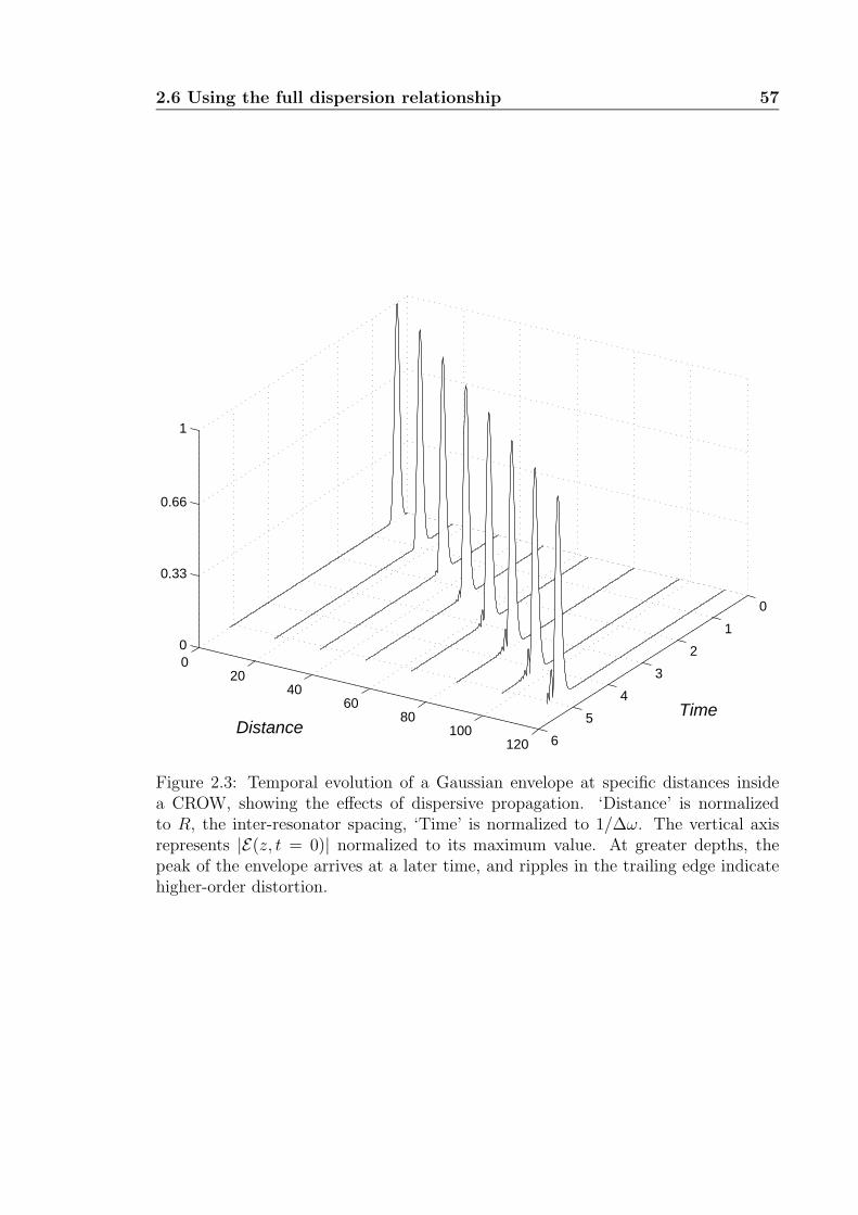
2.6 Using the full dispersion relationship 57
0
1
2
3
4
5
6
020
4060
80100
120
0
0.33
0.66
1
TimeDistance
Figure 2.3: Temporal evolution of a Gaussian envelope at specific distances insidea CROW, showing the effects of dispersive propagation. ‘Distance’ is normalizedto R, the inter-resonator spacing, ‘Time’ is normalized to 1/∆ω. The vertical axisrepresents |E(z, t = 0)| normalized to its maximum value. At greater depths, thepeak of the envelope arrives at a later time, and ripples in the trailing edge indicatehigher-order distortion.
58 Linear propagation in the tight-binding approximation
m and n in Eq. (2.57) by representing this condition as a Kronecker delta function.
After some algebra, we may write an expression for the envelope E(z, t) defined by
the usual relationship, |E(r, t)| ≡ exp[i(ω0t − k0z)]E(z, t), as the sum of two terms,
E(z, t) =1
4
z/R∑n=−∞
bn Jn(∆ωt) βz/R−n
∑l
ψl(z = 0)
+1
4
∞∑n=z/R
bn Jn(∆ωt) βn−z/R
∑l
ψl(z = 0),
(2.59)
where
bn =
2b0, n = 0
bn, n = 0.(2.60)
Note that this equates the magnitudes of the b’s, as a consequence of the original
definition, Eq. (2.58).
As functions of t, the first term on the right-hand side of Eq. (2.59) represents
a backward propagating pulse and the second term gives the forward-propagating
pulse. One way to see this is by using the fact that for small t, Jn(t) ∼ tn, so that as
we increase n, Jn(t) “rises from zero” at larger t. As z increases (and consequently
so does the integer, z/R), a larger n is required to maintain the same argument
of β in the second term of Eq. (2.59). Through its corresponding Bessel function,
this term will contribute significantly at larger t than a term involving a smaller n.
Physically, this describes a point on the envelope reaching greater values of z at later
t, i.e., a forward-propagating pulse. A similar argument shows that the first term in
Eq. (2.59), with the modified coefficients bn, describes a backward-propagating pulse.
A pulse envelope, as a function of t, is therefore described by a contiguous set
of Bessel functions: the field at z is written as a superposition of an appropriately
translated set of these functions Jz/R(t), Jz/R+1(t), . . ., multiplied by the coeffi-
cients β0, β1, . . .. Distortion accumulates with distance as a consequence of the
changing inter-relations between neighboring Bessel functions, e.g., the difference be-
tween the set J0(t), J1(t), . . . , Jp(t) and the set J5(t), J6(t), . . . , J5+p(t) for a given
β0, β1, . . .. Note that the Bessel functions are replaced by sinusoids in the limit of
a linear dispersion relationship in place of Eq. (2.8): these basis functions maintain
the same relationships between neighbors irrespective of the origin of the set, which
is why distortionless propagation may be achieved in this limit.
2.6 Using the full dispersion relationship 59
One additional simplification is illuminatory and may also considerably speed up
numerical computations. The normalizations in the identity [145]
n
∫ ∞
0
dx
xJn(bx) = 1, (2.61)
may be used in the definition of βn in Eq. (2.56). For slowly varying envelopes E(z =
0, t′), the asymptotic limit of the Bessel function is a cosine that, when multiplied by
a slowly varying function and integrated over several periods, averages out to zero.
We replace n/t′Jn(∆ωt′) with δ(t′ − n/∆ω) so that
βn = i−nE(z = 0, n/∆ω), n ≥ 1, (2.62)
i.e., the β’s represent temporal samples of the input pulse envelope along the ∆ωt axis.
The infinite summations in Eq. (2.59) may thereby be restricted to a finite number,
based on the temporal extent of the pulse, without significant loss of accuracy.
Further details may be found in [95, 87].
This analytical formulation allows waveguides to be designed to achieve
desired propagation characteristics. In a waveguide of a given length, the
inter-resonator spacing, which determines the parameters in Eq. (2.8),
may be chosen to limit the distortion, and achieve a certain (effective)
group velocity of propagation. Even though the dispersion relationship
is non-polynomial and nonlinear, this analysis yields a closed-form result
for arbitrary input pulse shapes, and to all orders of dispersion.
Waveguides constructed in electro-optically tunable material will allow the wave-
guide modes to be altered in realtime, through ψ(r) in Eq. (2.3), and consequently, the
eigenmode overlap integrals that appear in Eq. (2.8). Similar effects may be achieved
in MEMS waveguides constructed out of a patterned membrane with piezoelectric
actuators that cause a mechanical deformation; in this case, the physical geometry
of the resonators is altered rather than the refractive index difference between the
resonators and their surroundings. This leads to the development of microscale tun-
able all-optical delay lines and signal processing devices, such as interleavers and
multiplexers.

60 Linear propagation in the tight-binding approximation
Chapter 3
Two-pulse nonlinear interactions
...the powerful unified approach of coupled mode theory makesthe earlier analyses almost obsolete, and ... provides a
straighforward logical approach to the understanding of thephenomena and to the design of structures. In exchange for the
fascination and adventure of the historical approach to a new art,it provides the beauty and unity of a natural logical mathematical approach.
—C.C. Cutler, preface to W.H. Louisell, Coupled Mode andParametric Electronics, John Wiley & Sons (1960).
Among the most interesting applications of the framework of linear propagation of
pulses in the tight-binding method is a description of the basic nonlinear phenomena
in CROWs, such as second harmonic generation. Once we have a successful descrip-
tion of the “free” propagation of a CW field (a waveguide mode) or of a pulse (a
superposition of waveguide modes), it’s appropriate to attempt a description of the
effects of a nonlinear polarization generated in the waveguide, e.g., describing the
generation of a second harmonic field in a nonlinear CROW in the CW regime [150]
or using pulses [93]. The formalism presented here, based on [93], is central to the de-
scription of more complicated nonlinear phenomena, and is most generally described
as a coupled mode formalism of the time-dependent waveguide field distributions as
derived in Chapter 2. As in the previous chapter, we’ll consider the uniaxial propaga-
tion of pulses—along the z axis, to be specific. We do not discuss here any particular
features in the transverse geometry of the waveguide. As in the previous chapter,
we’ll restrict our discussion to modes of a particular parity.
There are certain general aspects of this investigation [93] that are important in
the discussion of any pulsed nonlinear phenomenon in the tight-binding analysis of
CROWs. A nonlinear polarization generated in the waveguide drives the evolution of
61
62 Two-pulse nonlinear interactions
the amplitude (envelope) of the waveguide mode, typically under the slowly-varying
envelope approximation (SVEA, which we maintain) [152]. The CW waveguide modes
which comprise a pulse [92] may each be assumed to be multiplied by an envelope
function, which complicates the analysis somewhat compared to the CW case. Fur-
thermore, an analysis of CW second harmonic generation in CROWs [150] that is not
prohibitively complicated relies on isolating the envelope of the waveguide mode from
the remainder of the field; the latter can be shown to follow the Bloch theorem [156].
Can such an approach be applied to the analysis of pulse propagation in the presence
of a nonlinear polarization? We’ll show that it can, although it requires a Bloch
function that depends both on spatial and temporal coordinates, in contrast with the
usual approach of a spatial Bloch function [94].
The efficiency of (unsaturated) second harmonic generation in a CROW with
CW waves is enhanced relative to that in bulk crystals by the inverse ratio of the
group velocities at the second harmonic frequency in the two waveguides [150], which
can approach 103 or 104 for weakly coupled CROWs [156]. It’s known that the
efficiency of second harmonic generation is enhanced at the band-edge of photonic
crystals, for exactly similar reasons of a reduction in the group velocity. Second
harmonic generation in a CROW combines this advantage with the enhancement
of the optical field found, e.g., in defect cavities in photonic crystals [143, 108]. A
numerical simulation of second harmonic generation with pulses in related structures
is presented in [120] and shows many features that are predicted by our analytical
formulation for this general class of structures.
The equations describing second harmonic generation in a CROW using pulses
rather than CW waves are formulated, allowing for a spatial and temporal variation
in the description of the rapidly varying part of the waveguide field distributions and
their envelopes.
3.1 Description of a pulse with an envelope in a CROW
A pulse is written as a superposition of waveguide modes, Eq. (2.32), with their
respective time evolution propagators,
E(z, t) =∑
allowed k’s
[coefficients]k eiω(k)tφk(z), (3.1)
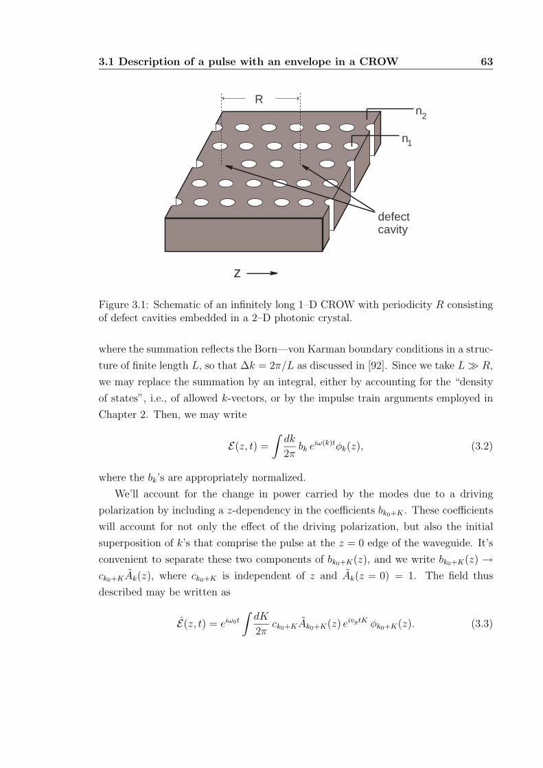
3.1 Description of a pulse with an envelope in a CROW 63
z
defectcavity
n
n
1
2
R
Figure 3.1: Schematic of an infinitely long 1–D CROW with periodicity R consistingof defect cavities embedded in a 2–D photonic crystal.
where the summation reflects the Born—von Karman boundary conditions in a struc-
ture of finite length L, so that ∆k = 2π/L as discussed in [92]. Since we take L R,
we may replace the summation by an integral, either by accounting for the “density
of states”, i.e., of allowed k-vectors, or by the impulse train arguments employed in
Chapter 2. Then, we may write
E(z, t) =
∫dk
2πbk eiω(k)tφk(z), (3.2)
where the bk’s are appropriately normalized.
We’ll account for the change in power carried by the modes due to a driving
polarization by including a z-dependency in the coefficients bk0+K . These coefficients
will account for not only the effect of the driving polarization, but also the initial
superposition of k’s that comprise the pulse at the z = 0 edge of the waveguide. It’s
convenient to separate these two components of bk0+K(z), and we write bk0+K(z) →ck0+KAk(z), where ck0+K is independent of z and Ak(z = 0) = 1. The field thus
described may be written as
E(z, t) = eiω0t
∫dK
2πck0+KAk0+K(z) eivgtK φk0+K(z). (3.3)
64 Two-pulse nonlinear interactions
As in Eq. (2.17), the coefficients ck0+K arise from a specified pulse shape at the
z = 0 edge of the waveguide and centered at the optical frequency ω0,
E(z = 0, t) = eiω0tE(z = 0, t), (3.4)
so that from the equality of Eq. (3.3) evaluated at z = 0 and Eq. (3.4), it follows that
ck0+K =1
φk0+K(0)
∫d(|vg|t′) E(z = 0, t′)e−ivgt′K . (3.5)
Combining Eq. (3.5) with Eq. (3.3), we may write
E(z, t) = eiω0t
∫d(|vg|t′) E(z = 0, t′)
∫dK
2π
φk0+K(z)
φk0+K(0)Ak0+K(z) eivg(t−t′)K . (3.6)
Eq. (3.6) may be simplified, based on the properties of a CROW. As represented
by Eq. (2.21), to leading order, 1/φ(0) ≈ 1, and using the explicit form for φk(z) in
Eq. (2.3),
E(z, t) =eiω0t∑
n
e−ik0nR∑
l
ψl(z − nR)
∫d(|vg|t′) E(z = 0, t′)
×∫
dK
2πAk0+K(z)eiTK ,
(3.7)
where T ≡ vg(t−nR/vg − t′). Using the following notation for the Fourier transform
relationship, ∫dK
2πAk0+K(z)eiTK = AT (z) ≡ A(z; T ), (3.8)
we can rewrite Eq. (3.7) as
E(z, t) =eiω0t∑
n
e−ik0nR∑
l
ψl(z − nR)
[∫
d(|vg|t′) E(z = 0, t′) A
(z; vg
[t − nR
vg
]− vgt
′)]
.
(3.9)
3.2 Representation in the Bloch form 65
3.2 Representation in the Bloch form
We see that the dispersion relationship, Eq. (2.14), dictates a temporal dependency
of the envelope A; however, if A were independent of K, then such would not be the
case. (As an aside, this shows that an assumption in Eq. (3.3) of an envelope of the
form Ak(z, t) would lead to overspecification.) The CROW dispersion relationship,
Eq. (2.14), doesn’t include group-velocity dispersion or higher-order dispersion terms,
and in many problems, the polarization term driving the evolution of the field may
be assumed to be constant over the relatively narrow range of propagation constants
k0 ± K that comprise the pulse in the center of the waveguide band. In such cases,
we would not expect a change in the temporal description of the envelope of the
pulse, since pulse envelopes of any shape (within certain parametric ranges related to
the sampling theorems (see Section 2.4) can propagate undistorted. It would seem
reasonable, therefore, to assume that the envelope A is indeed independent of the
propagation constant.
We can state these arguments and their consequences in the mathematical frame-
work of the previous section, assuming that the envelope is separable, A(z, t) =
α(z) ζ(t). Then, we may write
E(z, t) = α(z) eiω0t∑
n
e−ik0nR∑
l
ψl(z − nR)
∫dτ E(z = 0, τ/vg)
× ζ
[vg
(t − nR
vg
)− τ
],
(3.10)
or, in a more convenient form,
E(z, t) = α(z) ei(ω0t−k0z) uk0(z, t), (3.11)
where we define
uk0(z, t) ≡∑
n
eik0(z−nR)∑
l
ψl(z − nR)
∫dτ E(z = 0, τ/vg) ζ
[vg
(t − nR
vg
)− τ
].
(3.12)
Since the structure is infinitely long, the summation over n in Eq. (3.12) may
be translated as desired. We see that uk0(z + R, t + R/v) = uk0(z, t), and therefore
exp[i(ω0t − k0z)]uk0(z, t) is of the Bloch form (in spatial and temporal coordinates),
66 Two-pulse nonlinear interactions
i.e., a plane wave multiplying a function with an inherent periodicity reflecting that
of a lattice structure [9]. Consequently, E(z, t) may be viewed as an amplitude α(z)
modulating a Bloch wavefunction, uk0(z, t). This observation leads to a powerful and
general way to analyze nonlinear phenomena with pulses in CROWs [93], similar to
the analysis of cw phenomena [150].
Note that the spatial periodicity of the Bloch wavefunction is exactly that of the
CROW structure. The temporal periodicity is the time taken by the pulse envelope
to travel the distance defining the spatial periodicity. This is similar to the invariance
in the reference frame t − z/vg of the field envelope in weakly dispersive fibers and
semiconductor waveguides.
Further, since we’ve assumed Ak(0) = 1, we may use Eq. (3.8) and the consequent
observation α(z = 0) = 1 to write
ζ(T ) =
∫dK
2πeiTK = δ(T ), (3.13)
using the Dirac delta function. Therefore, the convolution integral in Eq. (3.12) can
be evaluated, and
uk0(z, t) =∑
n
eik0(z−nR)∑
l
ψl(z − nR) E
(z = 0, t − nR
vg
). (3.14)
An extension of Eq. (3.14) to three spatial dimensions (with pulse propagation
along the z axis) is straightforward, since the only vectorial functions are the modes
of the individual resonators, ψl(r). We’ll also generalize the notation from ω0 to ω,
since the description is equally valid at any carrier optical frequency, and from k0 to
k(ω), as the dispersion relationship dictates the propagation constant corresponding
to ω. (We’ll sometimes write kω in place of k(ω) so that the mathematical structure
of certain equations is not obscured.) In place of Eq. (3.14), we write
uk(ω)(r, t) =∑
n
eikω(z−nR)∑
l
ψl(r − nRez) E
(z = 0, t − nR
vg
). (3.15)
We can write the polarization in terms of this representation of the field describing
a pulse—an envelope modulating a spatio-temporal Bloch wavefunction—and thereby
obtain an evolution equation for the envelope.
3.3 Second harmonic generation: formulation 67
In characterizing the effects on pulse propagation of a polarization in a
coupled resonator optical waveguide (CROW), we’ve introduced a slowly
varying envelope for each of the waveguide modes comprising the pulse.
We’ve shown that the Ansatz of the envelope is strongly dictated by
the geometry of the waveguide. Under relatively mild assumptions, the
field distribution describing the pulse can be written as the product of a
spatial envelope function (which may in subsequent analyses be assumed
to be slowly varying if desired) and a wavefunction of the Bloch form,
i.e., a plane wave multiplying a periodic function. The periodicity of the
Bloch function depends both on spatial and temporal coordinates.
3.3 Second harmonic generation: formulation
The standard approach to second harmonic generation (SHG) in bulk crystals
accounts for the generation of the envelope of the second harmonic field as a con-
sequence of the nonlinear polarization in the medium using a formalism commonly
known as coupled-wave theory [126, 154]. The definition of the eigenmodes is from
the linear tight-binding equations, i.e., we don’t consider second harmonic generation
of intrinsically nonlinear pulseshapes such as solitons in this analysis. In bulk crys-
tals, the eigenmodes are usually of a simple form—exp[i(ωt−kz)]—and the resultant
equations for both CW waves and slowly varying envelope pulses are derived in [126,
Chap. 6–7]. In a CROW, the eigenmodes are more complicated as in Eq. (2.32), but
we’ve seenn that the analysis may be carried out on similar lines.
Based on the discussion in Section 3.2, we assume the following ansatz for the
second harmonic field distribution
E2(r, t) = E2(z) ei 2ωte−ik2ωzuk(2ω)(r, t), (3.16)
68 Two-pulse nonlinear interactions
so that the equation analogous to Eq. (2.40) is
v2
[4ω
c2− i
2
c2
∫d4r ε(r)
[uk(2ω)
]∗ · ∂uk(2ω)
∂t
]
=
∫d4r
[uk(2ω)
]∗ · [− 2k2ωez × [ezuk(2ω)]
− iez × [∇× uk(2ω)] − i∇× [ez × uk(2ω)]], (3.17)
where v2 ≡ d(2ω)/dk.
The nonlinear polarization PNL(r, t) generates the second harmonic field E2(r, t)
according to [154, 126, 57]
∇× [∇× E2] +ε(r)
c2
∂2E2
∂t2= − 1
c2
∂2
∂t2PNL(r, t). (3.18)
In Eq. (3.16), the exponential evolution factors and the Bloch wave function are all
explicitly dependent on spatial and temporal coordinates. Consequently, the algebra
is somewhat complicated and a table of vector identities is useful in simplifying the
component terms on the left-hand side of Eq. (3.18). We use the slowly varying
approximation [154, 126] to neglect the second-order derivatives of the envelope,
∣∣∣∣d2E2
dz2
∣∣∣∣ k2ω
∣∣∣∣dE2
dz
∣∣∣∣ , k2ω2 |E2| . (3.19)
The spatial derivatives can be written as
∇× [∇× E2] =ei 2ωte−ik(2ω)z
[i∂E2
∂z
− 2k2ωez × [ez × uk(2ω)]
− iez × [∇× uk(2ω)] − i∇× [ez × uk(2ω)]
+ E2
− k2ω
2ez × [ez × uk(2ω)] + ∇× [∇× uk(2ω)]
− ik2ω
[ez × [∇× uk(2ω)] − i∇× [ez × uk(2ω)]
] ],
(3.20)
3.3 Second harmonic generation: formulation 69
and the temporal derivatives can be written as
∂2E2
∂t2= ei 2ωte−iK(2ω)z
E2
[∂2uk(2ω)
∂t2+ i2(2ω)
∂uk(2ω)
∂t− (2ω)2uk(2ω)
]. (3.21)
We use Eq. (3.20) and Eq. (3.21) in Eq. (3.18) and use the eigenvalue equation for
uk(2ω) [analogous to Eq. (2.38)] to cancel certain terms. The result can be written as
idE2
dz
[− 2K2ωez × [ez × uk(2ω)] − iez × [∇× uk(2ω)] − i∇× [ez × uk(2ω)]
]= eiK(2ω)ze−i 2ωt
[− 1
c2
]∂2
∂t2PNL(r, t).
(3.22)
Next, we form the inner product of both sides of Eq. (3.22) with u∗k(2ω) and
integrate over t and r as in Eq. (2.36). Using Eq. (2.40) at the second harmonic
frequency, the left-hand side of Eq. (3.22), which we write as L, becomes
L = idE2
dzv2
[4ω
c2− i
2
c2
∫d4r ε(r)
[uk(2ω)
]∗ · ∂uk(2ω)
∂t
]. (3.23)
We simplify the right-hand side of Eq. (3.22) using Eq. (D.8) if we may assume
an undepleted fundamental, or using Eq. (D.9) otherwise. The differences between
the two cases are mostly notational and we’ll consider the former first. With the
following definitions,
∆kn ≡ k1(ω) + k2(ω) − k(2ω) + n2π
R,
p(r, t) ≡ uk1(ω)(r, t − z/v1)uk2(ω)(r, t − z/v1)(3.24)
forming the abovementioned inner product of the right-hand side of Eq. (3.22), which
we write as R, yields
R = − 1
c2E1
2
∫d4r e−i∆knzein 2π
Rz[uk(2ω)(r, t)
]∗ · d(r)[∂2p
∂t2+ 2i(2ω)
∂p
∂t+ (i 2ω)2p
].
(3.25)
From Eqs. (3.23) and (3.25), it’s clear that E2 will remain small unless there exists
an integer n such that ∆kn is very small. Then, exp(−i∆knz) is essentially constant
70 Two-pulse nonlinear interactions
over one unit cell and can be pulled out of the integral. Therefore,
R =4ω2
c2E1
2 e−i∆knz
[D(0)
n − i1
ωD(1)
n − 1
4ω2D(2)
n
], (3.26)
where
D(0)n ≡
∫d4r ein 2π
Rz[uk2(2ω)(r, t)
]∗ · d(r)uk1(ω)(r, t − z/v1)uk2(ω)(r, t − z/v1), (3.27)
D(1)n ≡
∫d4r ein 2π
Rz[uk2(2ω)(r, t)
]∗ · d(r)∂
∂t
[uk1(ω)(r, t − z/v1)uk2(ω)(r, t − z/v1)
],
(3.28)
D(2)n ≡
∫d4r ein 2π
Rz[uk2(2ω)(r, t)
]∗ · d(r)∂2
∂t2[uk1(ω)(r, t − z/v1)uk2(ω)(r, t − z/v1)
].
(3.29)
As discussed in Appendix D, we can extend the above analysis to allow for vari-
ations in the envelope of the fundamental, E1(r, t). We drop the factor of E12 in
Eq. (3.26) and instead define
p(r, t) ≡ E1(z)2uk1(ω)(r, t − z/v1)uk2(ω)(r, t − z/v1). (3.30)
We write down the equation that describes the evolution of the envelope of the sec-
ond harmonic mode at the frequency 2ω in its complete form for convenient reference
in subsequent analyses,
dE2
dz=
[i4ω
c2+
2
c2
∫d4r ε(r)
[uk(2ω)(r, t)
]∗ · ∂
∂tuk(2ω)(r, t)
]−14ω2
v2 c2
× e−i[k1(ω)+k2(ω)−k(2ω)+n 2πR ]z
∫d4r ein 2π
Rz[uk2(2ω)(r, t)
]∗ · d(r)
E1(z)2
[uk1(ω)(r, t − z/v1)uk2(ω)(r, t − z/v1) − i
ω
∫d4r ein 2π
Rz[uk2(2ω)(r, t)
]∗·d(r)
∂
∂t
[uk1(ω)(r, t − z/v1)uk2(ω)(r, t − z/v1)
]− 1
4ω2
∫d4r ein 2π
Rz
[uk2(2ω)(r, t)
]∗ · d(r)∂2
∂t2[uk1(ω)(r, t − z/v1)uk2(ω)(r, t − z/v1)
] ].
(3.31)
3.4 Solutions to the SHG equations 71
3.4 Solutions to the SHG equations
A closed form solution of Eq. (3.31) under general conditions is not known. In
this section, we’ll discuss certain simplifications which can lead to simple closed form
solutions that highlight the physics behind their formulation. These solutions demon-
strate a correspondence with known results in the theory of second-harmonic gener-
ation with CW waves [150].
As expected, dropping the time dependence and setting all time derivatives to
zero in Eq. (3.31) yields the equation for second harmonic generation with CW fields.
This is an ordinary differential equation for E2(z) and can be solved quite easily with
the assumption of an undepleted constant envelope fundamental. Cumulative growth
of the second harmonic field amplitude requires the phase matching condition,
k(2ω) = k1(ω)+k2(ω) + n2π
R
n = 0,±1,±2, . . .(3.32)
which explicitly involves the Bloch wave ‘vector’ n 2π/R.
Analytical time-dependent solutions may also be obtained under certain approx-
imations. We’ll continue to assume that E1 is constant (undepleted constant funda-
mental) and introduce the parameter p ≡ 1/(i 2ω). Using Eqs. (3.27)–(3.29), we can
write Eq. (3.31) as
v2dE2
dz= − E1
2
2p v2
[1 + p
∫d4r ε(r)
[uk(2ω)
]∗ · ∂
∂tuk(2ω)
]−1
× e−i∆knz[D(0)
n + 2pD(1)n + p2D(2)
n
].
(3.33)
For reasonably well-behaved picosecond pulses at the second harmonic [see Eq. (2.35)],
we may assume ∣∣∣∣p∫
d4r ε(r)[uk(2ω)
]∗ · ∂
∂tuk(2ω)
∣∣∣∣ 1. (3.34)
To see this, we refer to Eq. (2.35) and consider a Gaussian pulse at a second harmonic
frequency of 532 nm in a CROW, E2(z = 0, t) = exp(−t2/τ 2), where the pulse width
τ is 1 ps. Then, the left-hand side of Eq. (3.34) can be written as
1.8 × 10⁻¹⁵ s
(1 × 10⁻¹²)2 s2
∫dt
T2t
∫dr ε(r)
[uk(2ω)
]∗ · uk(2ω) ≤ 1.8 × 10⁻¹⁵ s
(1 × 10⁻¹²)2 s22T (3.35)
72 Two-pulse nonlinear interactions
since the range of t integration in Eq. (2.36) is over a time scale T . For picosecond
pulses, T is on the order of picoseconds, and therefore, the above number is on the
order of 10−2 or smaller.
The dominant contribution to second harmonic generation then follows the equa-
tiondE
(0)2
dz= − E1
2
2p v2
e−i∆knz[D(0)
n + 2pD(1)n + p2D(2)
n
]. (3.36)
Eq. (3.36) can be integrated to yield
E(0)2 (z)
∣∣∣z0
= −iE1
2ω
2v2
[D(0)
n + 2pD(1)n + p2D(2)
n
] [ 1
−i∆kn/2e−i∆knz
]∣∣∣∣z
0
. (3.37)
If we assume the usual boundary condition E(0)2 (z = 0) = 0, the envelope of the
second harmonic field distribution is
E(0)2 (z) = −i
[sin[∆knz/2]
∆knz/2
]e−i∆knz/2 z E1
2 ω
v2
[D(0)
n − i1
ωD(1)
n − 1
4ω2D(2)
n
]. (3.38)
The phase-matching sinc function in Eq. (3.38) is exactly analogous to the results
of CW second harmonic generation in bulk crystals, but with the definition of ∆kn
following Eq. (3.32). The condition ∆kn = 0 (for some n) is known as quasi-phase
matching [154, pp. 319–322] and reflects the important role of the waveguide geometry
on the efficiency of nonlinear processes.
Eq. (3.38) also shows that at the phase-matched condition, the intensity of the
second harmonic |E2|2 grows quadratically with distance z, the intensity of the fund-
mental |E1|2 and, in regions where it’s a constant, the nonlinearity coefficient d; these
are features in common with the analysis of second harmonic generation in bulk me-
dia [126]. As expected for an undepleted fundamental and linear propagation, the
boundary input propagates unchanged in shape, but delayed in time by z/v2 where z
is the length of the region under consideration and v2 is the group velocity of a pulse
at the second harmonic wavelength.
The linear growth of E(0)2 with z can’t persist indefinitely; saturation may be
accounted for by explicitly including the loss coefficient in the expression exp(−Γ2ω +
i 2ωt) in place of exp(i 2ωt) in Eq. (3.16). It may be seen that Eq. (3.38) is valid in
the regime z v2/Γ2ω [150].
In this regime, we can compute the efficiency of second-harmonic generation by
3.4 Solutions to the SHG equations 73
comparing the intensity at the second harmonic obtained from Eq. (3.38) to the power
flux of the fundamental. The electromagnetic energy density for the fundamental as
written in Eq. (D.2) is |E1|2ε(r)uk(ω)∗ · uk(ω). The group velocity v1 (the velocity of
energy flow) is intuitively defined as the ratio of the average power flow Pω to the
time-averaged energy stored per unit length, so that
Pω = v1
∫d4r ε
[uk(ω)
]∗ · uk(ω) =v1
R|E1|2 . (3.39)
Using Eq. (3.38), and assuming that the process is phase-matched and E2(z = 0, t)
is negligible,
P2ω(z) =v2
R
∣∣∣∣∣E12 1
v1 v2
ω R Pω z[D(0)
n − i1
ωD(1)
n − 1
4ω2D(2)
n
]∣∣∣∣∣2
. (3.40)
From Eqs. (3.39)and (3.40), the second harmonic generation efficiency at z = L is
η(L) =P2ω
Pω
=1
v12 v2
ω2 RPω L2∣∣∣D(0)
n − i1
ωD(1)
n − 1
4ω2D(2)
n
∣∣∣2. (3.41)
The factors of 1/v12 and 1/v2 show that the efficiency of second harmonic generation
is greatly increased by slowing down the propagation of pulses in the waveguide.
The equations describing sum-frequency generation in photonic crystal waveguides
with time-independent envelopes have been formulated by Sakoda et al. and solved
using a Green’s function [119, 118]. There are similarities between their analysis and
those in [150], and with the time-independent limit of this formulation. The expression
derived by Sakoda et al. for an “effective nonlinear susceptibility” in Eq. (19) of [119]
is similar to Eq. (3.27) and their final result Eq. (24) of [119] is similar to Eq. (3.38).
In particular, the enhancement of the field intensity by a factor 1/v2 as in Eq. (3.41)
and the conservation of crystal momentum ∆kn(z) = 0 are similar. We point out
that in contrast with Appendix A of [119], plane waves are not eigenfunctions of a
CROW and evaluation of the integrals in a Green’s function approach to the problem
may not be possible.
A numerical study of pulsed second harmonic generation in certain one-dimensional
periodic structures (dielectric stacks) was presented by Scalora et al. [120]. The prin-
ciple difference in their structure from a CROW lies in location of the dispersion
74 Two-pulse nonlinear interactions
curve in the band diagram: in the structure of Scalora et al., pulses are tuned to
the band edge, whereas in the case of the CROW, the defect cavity modes lie within
the bandgap, and pulse propagation results from the weak overlap of the spatial
distributions of these eigenmodes [150].
Although the physics behind the observations is different, there are several com-
mon phenomena such as a large reduction in the group velocity of pulse propagation
(when tuned to the appropriate part of the spectrum) and increased intensity in-
side the waveguide relative to free space. The plots of the ‘pump field eigenmode
distribution’ as numerically obtained by Scalora et al. [120, Fig. 4] from numerical
simulations also correspond closely to our theoretical formulation. This is a direct
consequence of the similarities in the geometrical structure of deep-grating photonic
bandgap structures [32] and a one-dimensional CROW.
Scalora et al. show that in the context of the slowly varying envelope approx-
imation as used here, the assumption of an undepleted fundamental is valid (i.e.,
negligible absorption is observed) and in this regime, the efficiency of second har-
monic is increased by orders of magnitude as predicted in Eq. (3.41). For certain
aspects of the problem, numerical simulations offer insight not yet available from
a theoretical investigation. As we have mentioned in Appendix C, the problem of
coupling a pulse into or out of such a strucure cannot be described as a Hermitian
eigenvalue problem. Scalora et al. demonstrate via simulations the importance of
the pulse width in coupling into such a structure—pulses with a spectral width larger
than that of the transmission resonance at the band-edge experience little field in-
tensity enhancement. It’s not clear at present if the bandwidth limitations that arise
from the discrete geometry of a CROW [92] are related to this phenomena.
The propagation and generation of a pulse as a consquence of a nonlinear
(second harmonic) polarization induced in a CROW is studied. We’ve
derived an approximate but analytical expression for the efficiency of
unsaturated second harmonic generation and have also shown how the
characteristics of the second harmonic pulse envelope in a CROW has
certain features in common with the well-known results in the generation
of second harmonic via CW waves in bulk crystals.
Chapter 4
Holography and four-pulse mixing
If one were running across the room in fast sixteenth notesand wanted to reduce them to eighths or quarters,
something would have to happen between the first and second of the slower notes ...or on the momentum generated by the fast notes, one would go flying through the wall ...
—Ralph Kirkpatrick, Interpreting Bach’s Well-Tempered Clavier, Yale (1984).
The interference pattern of two co-incident pulses in a nonlinear CROW creates an
index grating that may cause power transfer from one waveform to another—this is
known as two-beam coupling. Phenomena such as four-wave mixing and holography
involve a third waveform which is Bragg-scattered from this grating, resulting in the
generation of a fourth field that is related to the waveforms of the other fields. This
relationship is governed by energy and wavevector conversation, and by the material
properties of the medium.
The analysis of four-wave mixing is exactly analogous to that of holography, except
for the time coordinates—we’ll use the terminology interchangeably. We’ve obtained
the spatial Fourier transform (in K-space) of E(z, t) in Eq. (2.30). We will use the
symbols t′ and t to denote the temporal coordinates at the time of writing the holo-
gram and at the time of reconstruction, respectively. In general, t = t′ − T for
some time interval T . (As before, we’ll ignore the multiplicity of l values, assuming
that only a single mode from each of the individual resonators contributes to the
waveguide mode under consideration.) A typical geometry involves a grating writ-
ten by two counterpropagating pulses. We assume that two pulses E1(z = 0, t′) and
E2(z = L, t′) are input at the two opposite ends of a CROW. The pulses propagate
in opposite directions with wavevectors k1 and −k2 and group velocities v1 and v2,
respectively. The total field E(z, t′) is given by the sum of the fields due to these two
75
76 Holography and four-pulse mixing
pulses, and in K-space, can be written as
E(K, t′) =
eiω1t′∑
n
e−i(k1+K)nRψ(K)E1
(z = 0, t′ − nR
v1
)
+eiω2t′∑m
e−i(−k2+K)mRψ(K)E2
(z = L, t′ − mR
v2
) (4.1)
analogous to the K-space representation of a single pulse.
The interference pattern of the spectral components of this field (for example,
considering the component at K1 from the forward-propagating pulse and the com-
ponent at K2 of the backward-propagating pulse) is weighted by a complex coupling
coefficient δn(K1, K2) which depends on the material properties, the orientation of
the medium and the polarization of the waves [154, 123]. Therefore, we may write
the grating as
δn(z, t′) =1
F0
ei(ω1−ω2)t′∑n,m
∫dK1
2π
dK2
2πe−i(K1−K2)z e−i(k1+K1)nRe−i(−k2+K2)mR
× δn(K1, K2) E1
(z = 0, t′ − nR
v1
)E∗
2
(z = L, t′ − mR
v1
)
× ψ(K1)ψ∗(K2) + c.c.,
(4.2)
where F0 is the total optical power.
We assume that this grating persists for a certain amount of time, so that at a
later time t, δn(z, t) = δn(z, t′) and we can relabel the temporal coordinate t′ to t
in Eq. (4.2) to describe the reconstruction process. We will only focus on the term
in Eq. (4.2) written out in full, with the remark that analogous results hold for the
complex conjugate term (written in Eq. (4.2) as c.c.)1
We then use a backward-propagating reference pulse Er(z, t) to illuminate the
grating, and preserve its distinction from the reference pulse at the time of grating
formation E2(z, t) to maintain the generality of this discussion. At a later stage,
we’ll assume that these two pulses are in fact identical, and simplify the expressions
1This term will ultimately give rise to a field propagating in the direction opposite to that of E1,and is not of interest in this discussion.
77
appropriately. We can write Er(z, t) in the Fourier domain using Eq. (2.30),
Er(Kr, t) =
∫dKr
2πeiωrt
∑p
e−i(−kr+Kr)pRψ(Kr)Er
(z = L, t − pR
vr
). (4.3)
Upon illumination by Er(z, t), the polarization driving the propagation equa-
tion [154] for the reconstructed field Ec(z, t) is given in the instantaneous response
approximation by
Pc(z, t) = δn(z, t) Er(z, t). (4.4)
The evolution of the reconstructed field Ec(z, t) will follow that of the original signal
field E1(z, t) if this polarization Eq. (4.4) can be shown to be proportional to E1(z, t).
The multiplicative constant in this relationship includes the third-order susceptibil-
ity χ(3) rather than the linear susceptibility χ(1) since the grating δn(z, t) given by
Eq. (4.2) is proportional to the product of two optical fields [154].
We can multiply both sides of Eq. (4.4) by exp(−iKcz) and integrate over z
to write Eq. (4.4) in Fourier-transformed K-space. In doing so, we use Eqs. (4.2)
and (4.3) which describe the grating and the reference pulse, to obtain
Pc(Kc, t) =1
F0
ei(ω1−ω2+ωr)t∑n,m,p
∫dK1
2π
dK2
2π
dKr
2πδn(K1, K2)
∫dz ei(K1−K2+Kr−Kc)z
× e−i(k1+K1)nRe−i(−kr+Kr)pRei(−k2+K2)mRψ(K1) ψ(Kr) ψ∗(K2)
× E1
(z = 0, t − nR
v1
)Er
(z = L, t − pR
vr
)E∗
2
(z = L, t − mR
v2
).
(4.5)
The phase-matching integral over z can be approximated by 2π δ(K1−Kc)δ(K2−Kr) and we can carry out the integrals over K2 and K1. We write Kr ≡ K ′ and
Kc ≡ K to generalize the notation. In order to focus the discussion on holographic
reconstruction of the signal pulse, we now assume that Er(z = L, t) = E2(z =
L, t′)|t′=t, kr = k2, ωr = ω2 and vr = v2, i.e., we use a replica of the reference write-in
pulse E2 (in the original temporal coordinate t′) as the reference reconstruction pulse.
78 Holography and four-pulse mixing
Then, Eq. (4.5) becomes
Pc(Kc, t) =eiω1t∑
n
e−i(k1+K1)nRψ(K1) E1
(z = 0, t − nR
v1
)[1
2πF0
∫dK ′
2π
δn(K,K ′)∑m,p
e−i(−k2+K′)pRei(−k2+K′)mR ψ(K ′) ψ∗(K ′)
× E2
(z = L, t − pR
v2
)E∗
2
(z = L, t − mR
v2
)].
(4.6)
The term in square brackets in Eq. (4.6) can be written as
[· · · ] =1
2πF0
∫dK ′
2πδn(K,K ′) G(K ′, t)G∗(K ′, t), (4.7)
where
G(K ′, t) =∑
p
e−i(−k2+K′)pRψ(K ′)E2
(z = L, t − pR
v2
). (4.8)
Clearly, we can multiply G(K ′, t) by exp(iω2t) without changing Eq. (4.7).
Then, using the relationship established in Eq. (2.30),
Pc(K, t) = E1(K, t) × h(K, t), (4.9)
where
h(K, t) =1
2πF0
∫dK ′
2πδn(K,K ′) |E2(K
′, t)|2. (4.10)
We assume that the photorefractive properties of the CROW characterized by δn
are spectrally nonselective, i.e.,
δn(K,K ′) ≡ δn δ(K − K ′) for all K and K ′. (4.11)
Further, we assume that the (backward-propagating) reference pulses are narrow,
so that a fair mathematical approximation to the input free-space reference pulse
E2(z = L, t) is
E2(z = L, t) = eiω2tE0 δ (t − t0) . (4.12)
79
The corresponding field in the CROW is given by Eq. (2.30),
E2(K′, t) = E0e
iω2t∑m
ei(−k2+K′)mRψ(K ′) δ
(t − t0 − mR
v2
). (4.13)
Next, if the individual resonator modes are highly localized, ψ(z) = ψ δ(z − z0), we
can writeE2(K
′, t)E∗2 (K ′, t) = |E0|2 |ψ|2
∑m,m′
e−i(−k2+K′)(m−m′)R
×[δ
(t − t0 − mR
v2
)δ
(t − t0 − m′R
v2
)].
(4.14)
In order that power transfer over a significant time interval is cumulative, as given
by integrating the above expression over a region of t comparable to or greater than
R/v2, the term in square brackets in Eq. (4.14) can be replaced by the Kronecker
delta δmm′ , and the result is
E2(K′, t)E∗
2 (K ′, t) = |E0|2 |ψ|2M, (4.15)
where M is the number of resonators.
Using the normalization relationship M∫
dz |ψ(z)|2 = 1, we can simplify Eq. (4.10),
h(K, t) =1
(2π)2F0
δn |E0|2, (4.16)
which is a constant ≡ h, and therefore,
Pc(K, t) = h E1(K, t). (4.17)
This shows that the polarization term driving the evolution of the reconstructed
pulse is indeed proportional to the input signal pulse, as it would be for the input
signal pulse itself. Note that the scaling constant is dependent on the intensity of the
reference pulse, but for weak signal pulses, the total field intensity is dominated by
the reference and F0 ≈ |E0|2 so that the two factors cancel each other.
Photorefractive holography of single pulses has been difficult because of the low
efficiency of the process, and usually, multiple write-in procedures of thousands of
repeated pulses are necessary to obtain a sufficiently strong quasi-steady state grating.
In a CROW, the highly concentrated optical field can also enhance this aspect of the
80 Holography and four-pulse mixing
photorefractive effect. The propagating power flux P in a CROW is proportional to
the group velocity of the CROW band [156],
P =1
8πRvgE
20 , (4.18)
and therefore, we can obtain a higher optical field for a given power flux because of
the reduction in group velocity. Consequently, the time constant which determines
the photorefractive response time (and which varies linearly with the intensity [154])
is reduced by a factor vg ≈ 10−3 compared to the group velocity in a medium with
spatially uniform dielectric properties and refractive index n2. The quasi-steady state
equilibrium is reached with orders of magnitude lower intensities in a photorefractive
CROW as compared to a photorefractive bulk medium. As was pointed out by
Yeh [158], the fundamental limit on the speed of the photorefractive effect depends
on the intensity rather than phenomenological parameters induced by doping or heat
treatment.
We have analyzed optical pulse propagation in a coupled-resonator opti-
cal waveguide (CROW), and propose a new method for the storage and
reconstruction of optical pulses using photorefractive holography in a
CROW. The advantages of this method include a substantial reduction
in the group velocity leading to spatial compression of the signal pulse so
that it may be contained in a relatively short waveguide compared to the
spatial extent of the pulse in free space. The highly localized field dis-
tribution enhances the photorefractive effect, and we have examined in
detail the process of the formation of the grating and the reconstruction
of the signal pulse by holography. There are many possible applications
of such room-temperature, compact, nondestructive and low-intensity
pulse storage mechanisms; two important ones are buffers for optical
switches and correlators for optical measurement devices.
4.1 Applications: Nonlinear Delay Lines
In a 2–D periodic medium, such as a 2–D photonic crystal ‘slab,’ there are two
main types of waveguides: line defect waveguides, where a row of holes is filled in
4.1 Applications: Nonlinear Delay Lines 81
to create a guiding channel [78, 61], and via the coupling of resonator eigenmodes
of adjacent points defects which have been introduced in the desired geometry, e.g.,
the CROW. Although the physics behind waveguiding is quite different in these two
cases, they share the same spectrum of linear and nonlinear optics applications, e.g.,
guide light around sharp bends, highly selective spectral filtering, slowing down the
group velocity of light, efficient second harmonic generation, low-threshold lasing, etc.
In addition to these applications, which attempt to improve on existing methods of
carrying out the same functions in different geometries, these waveguides may realize
the proposals for new types of optical devices, with new functionalities in optical
communications. In particular, these structures offer the first practical possibility
to realize the proposal of ‘nonlinear optical delay lines’ (NLDL’s) [106], a class of
all-optical information processing devices at the mesoscopic and microscopic scale.
NLDL’s operate on the principle of the nonlinear interactions giving rise to power
transfer between several temporally encoded optical fields within a nonlinear medium.
Many of the important applications can be realized in two-wave or four-wave mixing
coupling processes, which we have investigated in the earlier sections. Photorefrac-
tive index gratings are an effective way to realize such effects with moderate intensity
levels, as would be necessary in practical applications. There are many applications
of NLDL’s in all-optical signal processing, including temporal multiplication, corre-
lation, and convolution, envelope time reversal, and space-to-time coding [106].
We will focus on photorefractive effects [154], but other grating mechanisms at a
variety of different timescales are also of potential interest, including free-carrier in-
dex gratings, acousto-optic standing waves, or arrays of nonlinear waveguides written
by spatial solitons. Such effects have been predicted to be particularly prominent in
coupled-defect waveguides, where the field intensity is highly localized to the individ-
ual resonators, and thereby locally enhancing the conversion to second-harmonic [150],
or reducing the build-up time of photorefractive gratings [91]. The effect of the spatial
localization of the field in such waveguides is related to the sampling theorems in com-
munications, and doesn’t invalidate the use of these waveguides if they’re designed
for the appropriate range of waveform parameters (temporal width of the envelope
and its spectral bandwidth) [92].
The second important requirement for the practical realization of NLDL’s is slow
group velocity, so that the grating written by the pulse envelopes can be completely
contained in the physical extent of the waveguide. In linear defect waveguides in
82 Holography and four-pulse mixing
photonic crystals, this can be achieved near the band edge [34], but at the cost
of distortion arising from higher-order dispersion terms in the the rapidly varying
dispersion relationship in this regime. In coupled-resonator waveguides (whether in
photonic crystals or not), slow group velocity can always be achieved more simply
as a natural consequence of the weak overlap between individual high-Q resonator
modes [150].
While so far, either class of waveguides can be considered as candidates for realiz-
ing NLDL’s, the fundamental physics of the grating dynamics preferentially indicates
the choice of coupled-resonator waveguides. We investigate the nonlinear coupling
processes between two pulses, rather than two cw beams, and the propagating en-
velopes in an infinitely long coupled-resonator waveguides have two length scales: an
overall envelope and a faster variation of the field distribution due to the quasi-discrete
nature of the physical structure. Temporal waveforms with two time scales incident
on a thin sample offer a closely related picture, with the advantage of being able
to monitor the dynamics of the grating on the shorter time scale using pump-probe
techniques. The material must be able to respond to the variations of the envelope on
the time-scale required for use in, e.g., a typical 10 Gbit/s communications system.
Considering at the physical aspects of such an experiment, the chosen material
may have a defect state at the wavelengths of interest, which we may or may not
want to use depending on the practical application. We have investigated a particular
geometry and used a material that permits both approaches, but these results refer
to a ‘direct’ two-photon process without an intermediate stage.
The theoretical formulation follows [26]. We consider the interaction of a two-
level system with a pulse, E(r, t) = eE(t) cos ω0t, where e describes the state of the
polarization, ω0 is the optical carrier frequency, and E(t) is the envelope. A two-level
atom (levels a and b) located at r = 0 interacts with this pulse.
We establish two times, t1 and t2, such that the envelope E(t) of width T is
contained in the interval (t1, t2). We’ll assume that the turn-on and turn-off time
intervals for E(t) are large compared to 1/ω0. We’ll also assume that T is large
enough for the validity of the S-matrix approach, i.e., longer than the lifetime of level
b.
The quantity we’re interested in is the S-matrix element
S = limt1→−∞, t2→+∞
< b | eiH0t2/U(t2, t1)e−iH0t1/ | a > (4.19)
4.1 Applications: Nonlinear Delay Lines 83
where U is the evolution operator for the a → b transition, and H0 describes the free
evolution of the atom outside (t1, t2) and is the atomic Hamiltonian in the absence of
an incident field.
Recall that the interaction Hamiltonian for a particle with charge q and mass m
in the presence of an external field described by potentials (A(r, t), U(r, t)) is [26,
p. 267],
H(I) = − q
mp · A(r, t) +
q2
2mA2(r, t) + qU(r, t). (4.20)
The last term is absent in this case. We assume that the levels a and b can’t be
connected via a one-photon transition (we’ll see shortly how this was realized exper-
imentally). We keep terms to order q2 in our calculation.
The second term of Eq. (4.20) doesn’t contribute, since it gives a term proportional
to <b | a>. The expansion of the first term of Eq. (4.20) to order q2 gives
S =( q
m
)2∫∫
dτ dτ ′ θ(τ − τ ′) eiωbτ∑
r
< b | p · A(0, τ) | r>
× e−iωr(τ−τ ′) <r | p · A(0, τ ′) | a > e−iωaτ ′.
(4.21)
The sum over r labels all possible intermediate levels—in our case, we will focus on
one particular value of r.
Dropping the nonresonant terms, and using the identity
e−i(ωra−ω)(τ−τ ′)θ(τ − τ ′) = − 1
2πi
∫ ∞
−∞dΩ
e−iΩ(τ−τ ′)
(Ω − ωra + ω0) + iε(4.22)
where ε → 0+, we can write
S =( q
m
)2pbrpra
i
∫ ∞
∞
E(Ω)E(ωba − 2ω0 − Ω)
4[(Ω − ωra + ω0) + iε], (4.23)
where E(Ω) ≡ 1/√
2π∫
E(t) exp(iΩt) dt is the Fourier transform of the envelope.
Since we’ve assumed that a one-photon transition is not resonant, and |ω0−ωra|
84 Holography and four-pulse mixing
1/θ where θ is the width of E(Ω), we can write
S =1
i
( q
m
)2 pbrpra
(ω0 − ωra)
∫ ∞
∞dΩ
E(Ω)E(ωba − 2ω0 − Ω)
4
=1
i
[( q
m
)2 pbrpra
(ω0 − ωra)
] ∫ ∞
∞dτ
[E(τ)
2
]2
ei(ωba−2ω0)τ .
(4.24)
The expression in square brackets outside the integral in Eq. (4.24) defines M , an
effective matrix element, so that we can simplify the notation:
S =1
iM
∫ ∞
−∞dτ
[E(τ)
2
]2
ei(ωba−2ω0)τ . (4.25)
This is the same expression we would’ve obtained for a one-photon transition, with
the change to [E(τ)/2]2 exp(−i2ω0t) for the field.
The transition amplitude depends on the square of the envelope rather than the
correlation at different times (or convolution for counterpropagating fields), since
there is no intermediate level for a one-photon process to occur. A classical treatment
of the formation of photorefractive gratings, with particular reference to coupled-
resonator waveguides, leads to similar conclusions with regard to the temporal de-
pendency [91].
4.2 Picosecond dynamics of photorefractive gratings in GaAs
But, while we can be certain that parasitic parameters do exist,their magnitude is usually not known, and even less do we know their ratios.
—A. A. Andronov, A. A. Witt, and S. E. Khaikin, Theory of Oscillators, Dover (1987).
We use 100 ps actively-mode-locked Gaussian pulses within a 270 ns Q-switched
envelope from a Nd:YAG laser emitting at 1.06 microns, as shown in Fig. 4.1. As
the photodiode had a bandwidth of a few gigahertz, an individual mode-locked pulse
cannot be resolved directly, but standard interferometry techniques can be used. The
setup is shown in Fig. 4.2. The pump and probe beam average powers were 1.5 W
and 15 mW, respectively. In light of Eq. (4.25), instead of the usual sample cut with
incident-face normal along [110] in the four-wave mixing geometry, we use a sample
with the surface-normal along [100]. The grating formed between the two co-polarized
pump beams will not transfer energy in the direction of the incident probe.
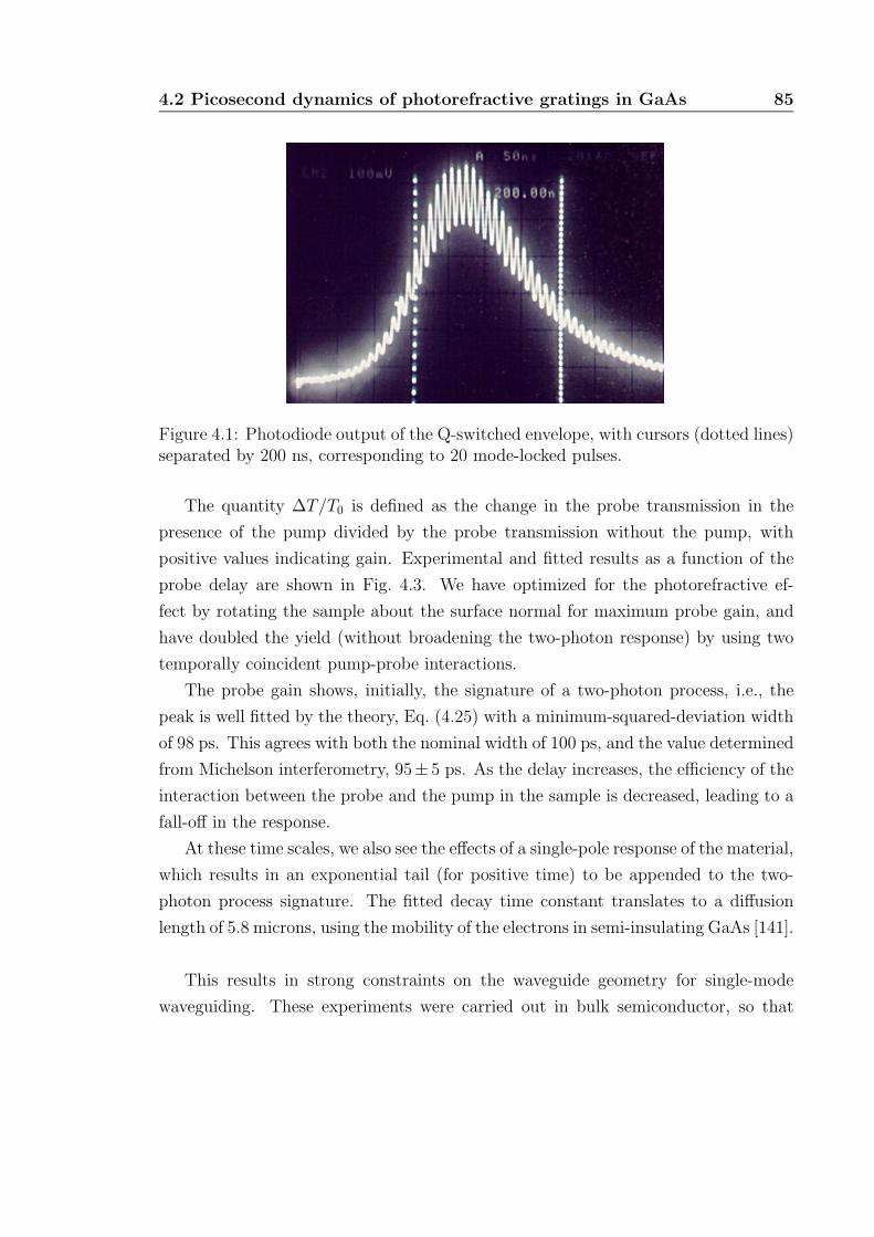
4.2 Picosecond dynamics of photorefractive gratings in GaAs 85
Figure 4.1: Photodiode output of the Q-switched envelope, with cursors (dotted lines)separated by 200 ns, corresponding to 20 mode-locked pulses.
The quantity ∆T/T0 is defined as the change in the probe transmission in the
presence of the pump divided by the probe transmission without the pump, with
positive values indicating gain. Experimental and fitted results as a function of the
probe delay are shown in Fig. 4.3. We have optimized for the photorefractive ef-
fect by rotating the sample about the surface normal for maximum probe gain, and
have doubled the yield (without broadening the two-photon response) by using two
temporally coincident pump-probe interactions.
The probe gain shows, initially, the signature of a two-photon process, i.e., the
peak is well fitted by the theory, Eq. (4.25) with a minimum-squared-deviation width
of 98 ps. This agrees with both the nominal width of 100 ps, and the value determined
from Michelson interferometry, 95± 5 ps. As the delay increases, the efficiency of the
interaction between the probe and the pump in the sample is decreased, leading to a
fall-off in the response.
At these time scales, we also see the effects of a single-pole response of the material,
which results in an exponential tail (for positive time) to be appended to the two-
photon process signature. The fitted decay time constant translates to a diffusion
length of 5.8 microns, using the mobility of the electrons in semi-insulating GaAs [141].
This results in strong constraints on the waveguide geometry for single-mode
waveguiding. These experiments were carried out in bulk semiconductor, so that
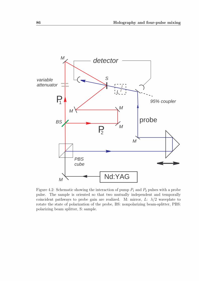
86 Holography and four-pulse mixing
probe
P1
detector
BS
PBScube
95% coupler
M
M
M
S
P2
Nd:YAG
L
M
variableattenuator
M
M
Figure 4.2: Schematic showing the interaction of pump P1 and P2 pulses with a probepulse. The sample is oriented so that two mutually independent and temporallycoincident pathways to probe gain are realized. M: mirror, L: λ/2 waveplate torotate the state of polarization of the probe, BS: nonpolarizing beam-splitter, PBS:polarizing beam splitter, S: sample.
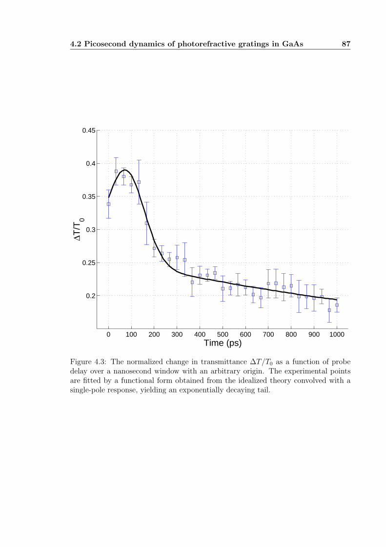
4.2 Picosecond dynamics of photorefractive gratings in GaAs 87
0 100 200 300 400 500 600 700 800 900 1000
0.2
0.25
0.3
0.35
0.4
0.45
Time (ps)
∆T/T
0
Figure 4.3: The normalized change in transmittance ∆T/T0 as a function of probedelay over a nanosecond window with an arbitrary origin. The experimental pointsare fitted by a functional form obtained from the idealized theory convolved with asingle-pole response, yielding an exponentially decaying tail.
88 Holography and four-pulse mixing
geometry-induced distortions to the write-read processes can be ignored 2. The finite
width of a waveguide—be it a line-defect waveguide in a photonic crystal slab or a
CROW—needs to be large compared to the diffusion length, otherwise the diffusing
carriers will be affected by the edges and the hologram will not faithfully reflect the
field envelope. A waveguide width of 6 µm is not single-moded at typical commu-
nications wavelengths (λ = 1.55 µm) for typical values of the dielectric constant in
semiconductor materials (GaAs, InGaAsP, etc.).
For these applications, a more suitable semiconductor would have a smaller dif-
fusion length, which would require a slower mobility for the electrons. At the same
time, we require that the photorefractive grating be established on the time-scales
of typical pulse envelopes as in this experiment. Of course, the material should be
optically transparent, and photorefractive, at these wavelengths. We don’t know of
a better choice than the GaAs family at the present time, but their limitations are
evident.
In light of these results, it’s unlikely that photorefractive holography is a practical
approach to realizing all-optical memory elements in CROWs at the bit rates of mod-
ern communication systems. The development of materials with faster reponses and
slower drift velocities may change this assessment. More promising is the approach
we’ll discuss in the next chapter: we can excite a localized envelope—a super-resonant
mode—in the CROW, which decays only with the time constant of the individual res-
onators. This stationary field distribution, rather than the propagating pulse, can be
used to form the hologram as discussed in this chapter: the advantage is that the
time constraints on the material response are considerably relaxed.
2Such perturbations can be considered, as in the analysis of noisy communication channels,as distorting filters so that the overall input-to-output response is the convolution of the transferfunctions of the undistorted holography and the nonidealities.
Chapter 5
The Kerr effect and super-resonant modes
Our basic dynamic variables shall be the vielbein and the connection.These superfields contain a large number of component fields.
Some will be eliminated through covariant constraintconditions. Others will be gauged away with (14.2).
In this way we shall arrive at a theory with the minimum number of component fields.
—J. Wess and J. Bagger, Supersymmetry and Supergravity, Princeton (1992).
As we’ve seen in Section 2.6, the dispersion relationship in CROWs is intrinsically
non-polynomial, but the propagation of localized excitations, i.e., optical pulses can be
characterized non-perturbatively to all orders of dispersion [95]. This is a somewhat
surprising result, and it leads to a description of the distortion that results from the
nonlinear dispersion relationship. Weighted sums of Bessel functions take the role of
cosines in the Fourier-series decomposition of the propagating field [87].
In optical fibers and similar waveguides, the effects of (anomalous) group-velocity
dispersion can be exactly balanced by the self-phase modulation induced by the Kerr
effect, an intensity-dependent change in the refractive index of the material. This is
the basis for the formation of the (fundamental) Schrodinger soliton in optical fibers,
for instance. Here, we investigate the Kerr effect in coupled-resonator waveguides,
with particular emphasis on determining whether self-phase modulation can com-
pensate for the distortion consequent of the nonlinear dispersion relationship. Such
solutions would lead to the existence of envelopes that can exist or propagate without
distortion in CROWs as eigensolutions of a nonlinear propagation equation (solitary
waves and solitons).
In considering the various choices of basis functions in which to expand the field,
we choose the propagating Bloch wave solutions of the CROWs without optical non-
linearities, which were derived using the tight-binding method in Chapter 2. We take
89
90 The Kerr effect and super-resonant modes
the field to be a superposition of such waves with slowly (time-) varying coefficients.
This expansion has the merit that in the absence of nonlinearities, each field in this
expansion is an eigenmode.
5.1 Formulation of the nonlinear propagation problem
In our treatment of linear pulse propgation in CROWs, we wrote the field describ-
ing a pulse E(r, t) as a superposition of waveguide modes φk(r) within the Brillouin
zone, and using Eq. (2.8),
E(r, t) ≈∫
dk
2πe−iωktckφk(r)
= e−iω0t
∫ π/R
−π/R
dK
2πe−i∆ωt cos[(k0+K)R]ck0+K φk0+K(r).
(5.1)
Since nonlinear phenomena such as the Kerr effect change the relative weights of
the eigenmodes Eq. (2.3) as the waveform evolves with time, it’s necessary to introduce
a time-dependency in the superposition coefficients ck appearing in Eq. (5.1). We
write
E(r, t) = e−iω0t
∫ π/R
−π/R
dK
2π
[e−i∆ωt cos[(k0+K)R]ck0+K(t) φk0+K(r)
]. (5.2)
We substitute Eq. (5.2) which describes the field in the waveguide in terms of the
time-varying coefficients ck0+K(t) into Maxwell’s equations written with an explicit
nonlinear polarization term describing the Kerr effect,
∇×∇× E(r, t) − µεwg(r)∂2
∂t2E(r, t) = µ
∂2
∂t2PNL(r, t) (5.3)
where
PNL(r, t) =3
4ε0χ
(3)|E(r, t)|2E(r, t). (5.4)
in the instantaneous response approximation.
In simplifying the terms, we use the normalization [91]
M∑m
∫dr εwg(r) |Eres(r − mRez)|2 = 1 (5.5)
5.1 Formulation of the nonlinear propagation problem 91
where the CROW waveguide comprises M resonators.
If we assume that ck0+K(t) varies slowly over time intervals ∼ O(2π/ω0), as is
usually the case, then we obtain
dck0+K(t)
dt= iγ
π/R∫∫−π/R
dK1
2π
dK2
2πexp
[− iκΩt
− cos[(k0 + K1)R] + cos[(k0 + K2)R]
+ cos[(k0 + K3)R] − cos[(k0 + K)R]]
ck0+K1(t)∗ck0+K2(t)ck0+K3(t) (5.6)
where K1+K = K2+K3 and γ is the nonlinearity coefficient in the CROW geometry,
defined as
γ = 2n0n2 ε0 ω0
∫dr∑m
|Eres(r − mRez)|4, (5.7)
using the relationship 3χ(3)/8 = n0n2 [4], and we have ignored the dispersion (varia-
tion in ω) of γ.
As an aside, Eq. (5.6) is equivalent to the differential equation
idan
dt+
∆α
2Ωan − κ
2Ω (an+1 + an−1) + γ|an|2an = 0, (5.8)
obtained by Christodoulides and Efremidis [24] for a related set of coefficients, an(t),
where
an(t) =
∫ π/R
−π/R
dK
2πck0+K(t) exp [in(k0 + K)R]
× exp
[i
∆α
2Ω − κΩ cos[(k0 + K)R]
t
].
(5.9)
The notational correspondence from our paper to theirs is (∆α/2)Ω → ∆ω and
−(κ/2)Ω → c. The an’s are the coefficients that appear in the expansion of the field
in terms of individual resonator modes, rather than the waveguide modes. It’s easily
verified that substituting the plane-wave ansatz, an = expi[(Ω − ωk0+K)t − (k0 +
K)nR] in Eq. (5.8) with n2 = 0 leads to the dispersion relationship, Eq. (2.8).
Returning our attention to Eq. (5.6), it’s useful to separate the amplitude and
phase of ck0+K(t),
ck0+K(t) = Ak0+K(t) exp[iφk0+K(t)]. (5.10)
92 The Kerr effect and super-resonant modes
We’ll look for solutions that retain their shape, i.e., dA/dt = 0. Substituting Eq. (5.10)
into Eq. (5.6) and separating the real and imaginary parts, we obtain a pair of equa-
tions,
dAk0+K
dt= −γ
∫∫dK1
2π
dK2
2πAk0+K1Ak0+K2Ak0+K3 sin Φ, (5.11)
dφk0+K
dt=
γ
Ak0+K
∫∫dK1
2π
dK2
2πAk0+K1Ak0+K2Ak0+K3 cos Φ, (5.12)
where Φ is defined as
Φ ≡− φk0+K1 − κ Ω t cos[(k0 + K1)R] + φk0+K2 − κ Ω t cos[(k0 + K2)R]+ φk0+K3 − κ Ω t cos[(k0 + K3)R] − φk0+K − κ Ω t cos[(k0 + K)R]
(5.13)
Based on Eq. (5.11), the A’s will be independent of t if sin Φ ≡ 0 for all t. This
implies that cos Φ = 1, and based on Eq. (5.12), we take φk0+K to be a linear function
of t,
φk0+K(t) = a + b t + κ Ω t cos[(k0 + K)R], (5.14)
where a and b are constants independent of t and K. We drop the constant a which
represents a fixed phase that can be absorbed into the initial conditions. Substituting
this form for φk0+K(t) into Eq. (5.12), we get
b + κΩ cos[(k0 + K)R] =γ
Ak0+K
π/R∫∫−π/R
dK1
2π
dK2
2πAk0+K1Ak0+K2Ak0+K3 . (5.15)
We’ll now discuss a particular regime in which there exist stationary (i.e., non-
propagating) solutions of Eq. (5.15). Such solutions utilize the optical Kerr effect to
exist stably in a confined section of the waveguide, isolated from the edges of the
structure.
5.2 The stationary super-resonant mode
In this section, we investigate in what regime the nonlinear CROW admits solu-
tions of the Schrodinger soliton form, i.e., the hyperbolic secant. The basic physics
reflects a balance between the phase modulation effects of the Kerr effect and (anoma-
5.2 The stationary super-resonant mode 93
lous) group-velocity dispersion (GVD). The GVD term in the nonlinear Schrodinger
equation appears as the coefficient of a second derivative term, which in the Fourier
domain with the Fourier (frequency) variable K, translates to multiplication by (iK)2.
In Eq. (5.15), if we assume that k0R is a multiple of 2π and |KR| 1, then
we may write cos[(k0 + K)R] ≈ 1 − (KR)2/2, which is the desired effective GVD
term. Observe from the dispersion relationship, Eq. (2.8), that ωk0+K is a quadratic
function of K only at the edges of the Brillouin zone, where dωk0+K/dK vanishes, i.e.,
the group velocity is zero. We expect, therefore, that the solutions of Eq. (5.15) in
this regime will be stationary , describing a localized state that is frozen in its initial
(t = 0) spatial distribution and does not propagate along the waveguide.
Using this approxmation, Eq. (5.15) becomes
b + κΩ = κΩ(KR)2
2+
γ
Ak0+K
π/R∫∫−π/R
dK1
2π
dK2
2πAk0+K1Ak0+K2Ak0+K3 . (5.16)
We’ll assume that the A’s are defined to be zero outside the regions of integration
−π/R and π/R so that the limits of integration can be taken as −∞ to ∞. Eq. (5.16)
may then be solved [109],
Ak0+K = A(0)k0+K sech(K/K), (5.17)
where K is a spectral width parameter whose relevance will become clear in the
following discussion. Substituting Eq. (5.17) into Eq. (5.16), we get
b + κΩ = κΩ(KR)2
2+ 2
[A
(0)k0+K
]2 γ
(2πR)2
[(KR)2 +
(πKR
2
)2]
. (5.18)
If b is to be independent of K, then we need
A(0)k0+K =
√−(2πR)2κΩ
4γ. (5.19)
Since the left-hand side represents a real and positive number, we require that κ as
defined in Eq. (2.9) be a negative number (as is physically expected from the meaning
of εwg and εres). This is equivalent to anomalous dispersion in optical fibers and similar
94 The Kerr effect and super-resonant modes
waveguides.
Using Eq. (5.14) and Eq. (5.19) in Eq. (5.10), we write the final expression for
ck0+K(t),
ck0+K(t) = ck0+K(0) exp− iκΩt
[1 + π2(KR)2/8 − cos(KR)
], (5.20)
where
ck0+K(0) ≡ 2πR
√−κΩ
4γsech(K/K), |KR| ≤ π. (5.21)
The field described by these coefficients is
E(r, t) = e−iω0te−iκΩt[1+π2(KR)2/8]∫ π/R
−π/R
dK
2πck0+K(0) φk0+K(r). (5.22)
In light of Eq. (5.21), the integral on the second line of Eq. (5.22) is not expressible in
a simpler form. However, if KR 1, the hyperbolic secant function decays rapidly,
and the limits of integration may be changed to (−∞,∞). The integral then can be
evaluated easily—the Fourier transform of a hyperbolic secant is itself a hyperbolic
secant function. We derive the approximation,
E(r, t) ≈ e−iω0te−iκΩt[1+π2(KR)2/8]
√−κΩ
4γπKR
∑n
sech
(πK
2nR
)Eres(r − nRz).
(5.23)
The modulus of the amplitude |E(z, t = 0)| normalized to its maximum value (in
this approximation) is plotted in Fig. 5.1. Values of the hyperbolic secant function
in Eq. (5.23) at nR (which has the dimensions of length) are the weights of the
individual resonator eigenmodes. In this approximation, the envelope of these weights
is a hyperbolic secant function whose width is inversely proportional to K.
As we had expected from physical arguments, the envelope of E(r, t) is a station-
ary state that is independent of time: its spatial distribution at t = 0 is of finite
extent and is maintained for all subsequent t. This is consistent with the observation
that although the group velocity dispersion coefficient is nonzero, the group velocity
itself is zero. We call the stationary state a super-resonant field since it is formed
in a waveguide that itself comprises the coupling of individual (stationary) resonator
modes. There are two requirements for such a solution: (1) the slowly varying as-
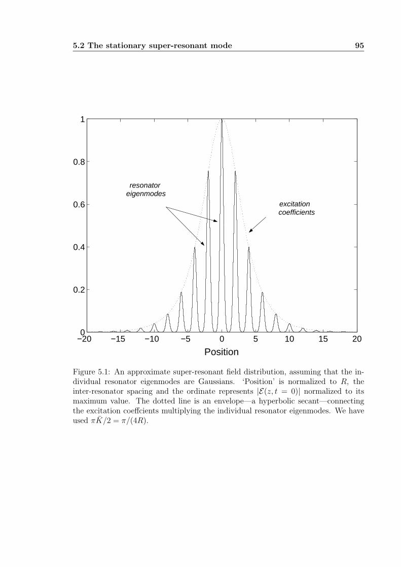
5.2 The stationary super-resonant mode 95
−20 −15 −10 −5 0 5 10 15 200
0.2
0.4
0.6
0.8
1
Position
resonator eigenmodes
excitation coefficients
Figure 5.1: An approximate super-resonant field distribution, assuming that the in-dividual resonator eigenmodes are Gaussians. ‘Position’ is normalized to R, theinter-resonator spacing and the ordinate represents |E(z, t = 0)| normalized to itsmaximum value. The dotted line is an envelope—a hyperbolic secant—connectingthe excitation coeffcients multiplying the individual resonator eigenmodes. We haveused πK/2 = π/(4R).
96 The Kerr effect and super-resonant modes
sumption, which simplifies Eq. (5.22) to Eq. (5.23) and (2) the necessary condition
that k0R is an integer multiple of 2π.
Using Eq. (5.9), Eq. (5.23) may be rephrased as an expression for the individual-
resonator coefficients an(t),
an(zn) =
[√−κΩ
4γπKR
]e−iµt sech
(πK
2zn
), (5.24)
where µ ≡ κΩ[1 + π2(KR)2/8
]is a constant frequency detuning and zn ≡ nR is a
discretization of the spatial axis.
Christodoulides and Efremedis [24] have analyzed this problem using the an coef-
ficients, and have derived the expression (in our notation),
an(zn, t) =
[√−κΩ
4γπKR
√cos q
]e−iµt cos q sech
[πK
2(zn − v t)
], (5.25)
which described an envelope that propagates with the group velocity v ≡ −κΩR sin q
defined in terms of an undetermined parameter q in their analysis. The solution
Eq. (5.25) for nonzero v is derived from a nonlinear Schrodinger equation, which
involves linear dispersion and quadratic terms only. There’s no such point on the dis-
persion relationship, Eq. (2.8) and the validity of this approximation is questionable.
In fact, the dispersion relationship is quadratic only at the edges of the Brillouin
zone where the group velocity goes to zero. A quadratic dispersion relationship is
what is needed to have exact hyperbolic-secant solutions of the nonlinear Schrodinger
equation: the presence of higher-order dispersion doesn’t lead to this form [4].
We’ve investigated the effects of the optical Kerr nonlinearity in coupled-
resonator optical waveguides (CROWs) with regard to the propagation of
optical pulses. In particular, there exists a stationary field distribution of
the hyperbolic secant form which balances the effects of group velocity
dispersion and the Kerr self-phase modulation. This field distribution
remains frozen in space with zero group velocity.
The super-resonant mode in a CROW composed of high-Q resonators can have a
long lifetime, since it decays with the time constant associated with the quality factor
5.2 The stationary super-resonant mode 97
of the isolated individual resonators [150] rather than the time constant associated
with the coupling between high-Q resonators and external waveguides. In addition,
an optical pulse (with nonzero group velocity) traveling down the waveguide can be
made to interact with such a static distribution; their interaction can be enhanced
using quasi-phase-matching (grating) techniques, [91]. This leads to the possibility
of the application of these localized states as memory elements in optical switches,
particularly in conjunction with the photorefractive holography processes discussed
in Chapter 4.
The general phenomenon of the localization of light is not necessarily a conse-
quence of defects in a uniform photonic crystal. In the presence of optical (electromag-
netic) nonlinearities, intrinsic localized modes or discrete breathers can be formed [86].
This has has been proven mathematically for using a class of time-periodic, spatially
localized solutions to a Hamiltonian coupled-oscillator nonlinear lattice [80]. Discrete
breathers have been predicted for 2–D and 3–D photonic crystals with Kerr (cubic)
nonlinearity [59], at nonlinear interfaces with quadratic nonlinearity [132] and along
dielectric waveguide structures with a nonlinear Kerr-type response [85].
A waveguide that, unlike a CROW, exhibits continuous translational symmetry
in the longitudinal z direction, and in the transverse plane, consists of an array
of thin quadratically nonlinear layers embedded in a linear slab waveguide, can
inhibit light propagation along the transverse x axis under certain conditions [133].
“Two-color” spatially localized nonlinear modes can be formed as a consequence of
parametric coupling of the fundamental and second-harmonic fields excited at the
nonlinear interfaces. Such modes are related to spatial quadratic solitons that are
localized in homogeneous media by two-wave parametric mixing of the fundamental
and the second-harmonic waves [64].
A related structure is a one-dimensional grating consisting of χ(2) material.
Forward- and backward-propagating waves of the fundamental frequency and the
second-harmonic interact via terms reminiscent of the cubic Kerr effect. This gives
rise to localized slowly moving two-color envelopes, on picosecond timescales for
fundamental beam intensities of approximately 10 GW/cm2 in LiNbO3 [27]. What
is especially interesting is that the second-harmonic beam is locally generated in the
backward direction, but its envelope is locked to the forward-propagating fundamen-
tal frequency component—it also travels forward.
The interface between two semi-infinite bulk optical media with inversion sym-
metry breaks the inversion symmetry, and consequently possesses a nonzero surface

98 The Kerr effect and super-resonant modes
quadratic response. Recent experiments on second-harmonic generation in periodic
photonic bandgap structures with embedded nonlinear defect layers have observed
enhanced parametric interaction in the vicinity of these defects [138]. This suggests
that second-harmonic generation occurs in localized modes, but is suppressed for
propagating modes [133].
Chapter 6
Dispersion-managed solitons and breathers
... the variational principle is generally useful in unifyinga subject and consolidating a theory rather than in breaking ground
for a new advance ... This is not to minimize the importance of findingthe Lagrange density L, for ... the form of the variational equations
often suggests fruitful analogies and generalizations.
—P. M. Morse and H. Feshbach, Methods of Theoretical Physics, McGraw-Hill, 1953.
Nonlinear pulses, such as solitons [44, 51], are intuitively the pulse envelopes of
choice in high bit-rate optical communications, since they are solutions to the enve-
lope propagation equation accounting for both the dispersion and the nonlinearity of
optical fibers. Some of the principal objections (conceptual and practical) to the pro-
posals of repeaterless long-haul soliton communication systems have been addressed
by the introduction and development of dispersion-managed (DM) solitons [128, 134],
and it is expected that such systems will be used as the primary means of optical
transport beyond 40 Gbit/s per wavelength-division multiplexing (WDM) channel
(recent review papers on the theory and experiments of solitons and DM solitons
include [43] and [103]).
The slowly varying normalized envelope u(z, t) of an optical pulse in a lossless
single-mode fiber with dispersion management in the group-velocity dispersion pa-
rameter and third-order dispersion follows the nonlinear Schrodinger equation derived
in Eq. (1.27),
i∂u
∂z+
σ(z)
2
∂2u
∂t2+ |u|2u − iγ
∂3u
∂t3= 0, (6.1)
where t is the temporal coordinate in the moving reference frame, and is defined with
respect to the laboratory space and time coordinates z and T by the equation t =
T − z/vg, where vg is the group velocity of the pulse. As discussed in Section 1.4, the
99
100 Dispersion-managed solitons and breathers
parameters σ and γ are functions of the propagation distance z; in a later section, we
will focus on pulse propagation characteristics in a piecewise constant (step-function)
dispersion map σ(z) = σ±, with σ+ > 0 > σ−, and periodicity σ(z) = σ(z + zT ).
Recent studies on the use of solitons in dispersion-managed optical communica-
tions systems have shown that the effect of third-order dispersion, which arises from
d3β/dω3 where β(ω) is the mode propagation constant at optical frequency ω, may
be significant since the average group-velocity dispersion can be much lower than the
local group-velocity dispersion.
We derive explicit analytical expressions for the dynamic behavior of soliton-like
pulses (breathers) in such a system. Nonperturbative Lagrangian and Hamiltonian
formulations have been useful in understanding the physical behavior of propaga-
tion in systems characterized by second-order dispersion alone [68]. This work forms
a counterpart to the perturbative analysis of Lakoba and Agrawal [72] based on a
Hermite-Gaussian expansion of the pulse shape. The analysis presented here should
also help understand the physical origins of certain features found in numerical sim-
ulations of the effects of third-order dispersion [38]. Since the nonlinear (noninte-
grable [71]) partial differential (wave) equation is now of a higher order, it may be
useful to show the applicability of a mathematical technique that is easily understood
and widely used in a different problem.
We limit our attention to the steady-state (asymptotic) behavior of such pulses,
and therefore neglect the effect of continuum radiation on the dispersion-managed
breather [72]. A soliton losing energy to linear dispersive waves in the normal disper-
sion regime “recoils” further into the anomalous regime of the spectrum [6]. This
lowers the radiation amplitude, which arises as a consequence of the tail of the
soliton spectrum in the normal dispersion regime. It can then be expected that a
quasi-stationary state is reached where the radiation rate is so small that the soliton
recoil is negligible, and we can ignore further radiation losses. Further, a practical
communication system using dispersion management is likely to use optical filters
and band-limited amplifiers, which can suppress out-of-band dispersive radiation and
frequency shifts due to spectral recoil [140].
Consequently, we are justified in assuming a symmetrical pulse shape. Given
that we do not predict the generation of any new harmonics in this approximation,
we would not expect any associated frequency shift; indeed this will be shown to
be a conserved quantity (as a generalized momentum canonically conjugate to a
6.1 Lagrangian and Hamiltonian formulation 101
cyclic coordinate). It is interesting to note that the perturbative approach used
by Lakoba and Agrawal [72] also does not predict any frequency shift for the lossless
case considered here.
We quantify our results in terms of a representative hyperbolic secant pulse shape,
but the method can be generalized to a number of different (localized) pulse shapes,
e.g., Gaussian, triangular, etc. An appropriate Lagrangian is constructed for the
nonlinear Schrodinger equation, and the condition of its extremality with respect to
our pulse Ansatz forms variational equations of motion for the pulse parameters [7].
Identifying generalized coordinates and their conjugate momenta leads to the Hamil-
tonian and a phase-plane analysis in terms of the acyclic coordinates. We highlight
the modifications brought about by third-order dispersion to the well-known results
of second-order dispersion-managed propagation.
6.1 Lagrangian and Hamiltonian formulation
The partial differential equation (6.1) and its conjugate can be reduced to a system
of ordinary differential equations using the averaged variational method, first intro-
duced in the context of the evolution of solitons by Anderson [7]. The motivation
for this approach is well known and we shall only point out that in the presence of
third-order dispersion, the final term in (6.1) modifies the Euler-Lagrange equation,
δLδu
≡ ∂L∂u
− ∂
∂t
∂L∂(∂u/∂t)
− ∂
∂z
∂L∂(∂u/∂z)
+∂2
∂t2∂L
∂(∂2u/∂t2)= 0 (6.2)
and similarly for u∗ in place of u.
It may be easily verified, e.g., by direct substitution, that the following Lagrangian
density (assumed to be at least C1 in u and its derivatives, except possibly on a set
of measure zero) satisfies this condition,
L(u, u∗) = i
(u∂u∗
∂z− u∗∂u
∂z
)+ σ(z)
∣∣∣∣∂u
∂t
∣∣∣∣2
− |u|4 − iγ
(∂2u
∂t2∂u∗
∂t− ∂2u∗
∂t2∂u
∂t
), (6.3)
where a piecewise continuous σ(z) satisfies the condition in parentheses.
The pulse shape we choose to base our analysis on should be capable of predicting
pulse evolution, and therefore, in view of the term in (6.3) that contributes to third-
102 Dispersion-managed solitons and breathers
order dispersion, we have to choose a pulse shape (envelope) somewhat more involved
than for second-order dispersion alone [68]. We take
u(z, t) = A√
η sech [η(t − c)] exp
[i
(Ω(t − c) + β(t − c)2 +
φ
2
)], (6.4)
where η, β, Ω, c and φ are free parameters that depend on z and represent the
amplitude (and width), quadratic chirp, frequency shift from the carrier frequency
(or velocity), pulse center in the moving reference frame (or group-velocity variation
in laboratory coordinates) and phase, respectively. In the interests of legibility, we
will not write out this dependence explicitly. The pulse energy is then evaluated to
∫ ∞
−∞dt u(z, t)∗.u(z, t) = 2A2. (6.5)
Similar forms of the envelope Ansatz have been used elsewhere [56] for analyzing
pulse interactions in second-order dispersion-managed systems, and reflect the fact
that the equations under consideration need more degrees of freedom than offered by
simpler assumptions.
We now write down the Lagrangian using (6.3) and (6.4). A fair amount of algebra
leads to the following expressions for the four terms on the right-hand side of (6.3),
where we use the shorthand β′ ≡ dβ/dz, etc.
i
(u∂u∗
∂z− u∗∂u
∂z
)→ 2
[(t − c)2β′ + (t − c)(Ω′ − 2βc′) + (φ′ − Ωc′)
]u∗u,
σ
∣∣∣∣∂u
∂t
∣∣∣∣2
→ σ[4(t − c)2β2 + η2tanh[η(t − c)]2
+4(t − c)βΩ + Ω2]u∗u,
−|u|4 → −A2η sech[η(t − c)]2u∗u,
−iγ
(∂2u
∂t2∂u∗
∂t− ∂2u∗
∂t2∂u
∂t
)→ γ
[16(t − c)3β3 + 24(t − c)2β2Ω + 2Ω(η2 + Ω2)
−2β[η tanh[η(t − c)] − (t − c)(η2 + 3Ω2)
]]u∗u.
(6.6)
In each of the above expressions, we can drop those terms that are odd in t as
such terms do not contribute when multiplied by u∗u and integrated over t. These
6.1 Lagrangian and Hamiltonian formulation 103
include terms that are proportional to odd powers of (t − c) and those that vary as
tanh(t − c). After some simplification, we can write the Lagrangian as
L = A2
π2
3η2
dβ
dz+ 4
(dφ
dz− Ω
dc
dz
)− 4A2η
3+ 2σ
[Ω2 +
1
3
(π2β2
η2+ η2
)]
+4γΩ
[π2β2
η2+ Ω2 + η2
]. (6.7)
with a clearly nontrivial role for γ. The Lagrangian function (6.7) has no explicit z
dependence, and so the Hamiltonian is a constant of the motion. This will be the
starting point of our discussion in the following section.
We note in passing that it is possible to construct a Lagrangian for pulse shapes
other than the hyperbolic secant reminiscent of the Schrodinger soliton, generalizing
to any localized Ansatz for which the amplitude and pulse width are related in the
same way as above.
We apply the Legendre transformation [121] to the Lagrangian (6.7) to generate
the Hamiltonian. We take our canonical coordinates as β and c with conjugate
momenta
pβ =∂
∂β′L =π2A2
3η2,
pc =∂
∂c′L = −4A2Ω (6.8)
and express the Lagrangian in terms of these variables, substituting pβ for η and pc
for Ω,
L = A2
γpc
(p2
c
16A6+
π2
3pβ
+3pββ2
A4
)+ σ
(2π2A2
9pβ
+p2
c
8A4+
2pββ2
A2
)
− 4πA3
3√
3pβ
+ 4dφ
dz
+ pββ′ + pcc
′. (6.9)
(It can be verified after extensive algebra (symbolic manipulation tools such as Math-
ematica are useful) that det(∂2L/∂pi∂pj) = 0.)
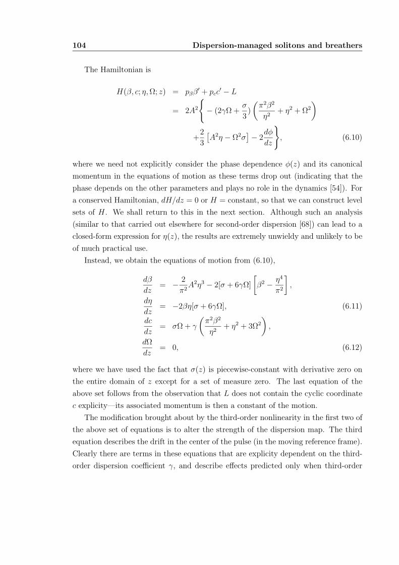
104 Dispersion-managed solitons and breathers
The Hamiltonian is
H(β, c; η, Ω; z) = pββ′ + pcc′ − L
= 2A2
− (2γΩ +
σ
3)
(π2β2
η2+ η2 + Ω2
)
+2
3
[A2η − Ω2σ
]− 2dφ
dz
, (6.10)
where we need not explicitly consider the phase dependence φ(z) and its canonical
momentum in the equations of motion as these terms drop out (indicating that the
phase depends on the other parameters and plays no role in the dynamics [54]). For
a conserved Hamiltonian, dH/dz = 0 or H = constant, so that we can construct level
sets of H. We shall return to this in the next section. Although such an analysis
(similar to that carried out elsewhere for second-order dispersion [68]) can lead to a
closed-form expression for η(z), the results are extremely unwieldy and unlikely to be
of much practical use.
Instead, we obtain the equations of motion from (6.10),
dβ
dz= − 2
π2A2η3 − 2[σ + 6γΩ]
[β2 − η4
π2
],
dη
dz= −2βη[σ + 6γΩ], (6.11)
dc
dz= σΩ + γ
(π2β2
η2+ η2 + 3Ω2
),
dΩ
dz= 0, (6.12)
where we have used the fact that σ(z) is piecewise-constant with derivative zero on
the entire domain of z except for a set of measure zero. The last equation of the
above set follows from the observation that L does not contain the cyclic coordinate
c explicity—its associated momentum is then a constant of the motion.
The modification brought about by the third-order nonlinearity in the first two of
the above set of equations is to alter the strength of the dispersion map. The third
equation describes the drift in the center of the pulse (in the moving reference frame).
Clearly there are terms in these equations that are explicity dependent on the third-
order dispersion coefficient γ, and describe effects predicted only when third-order
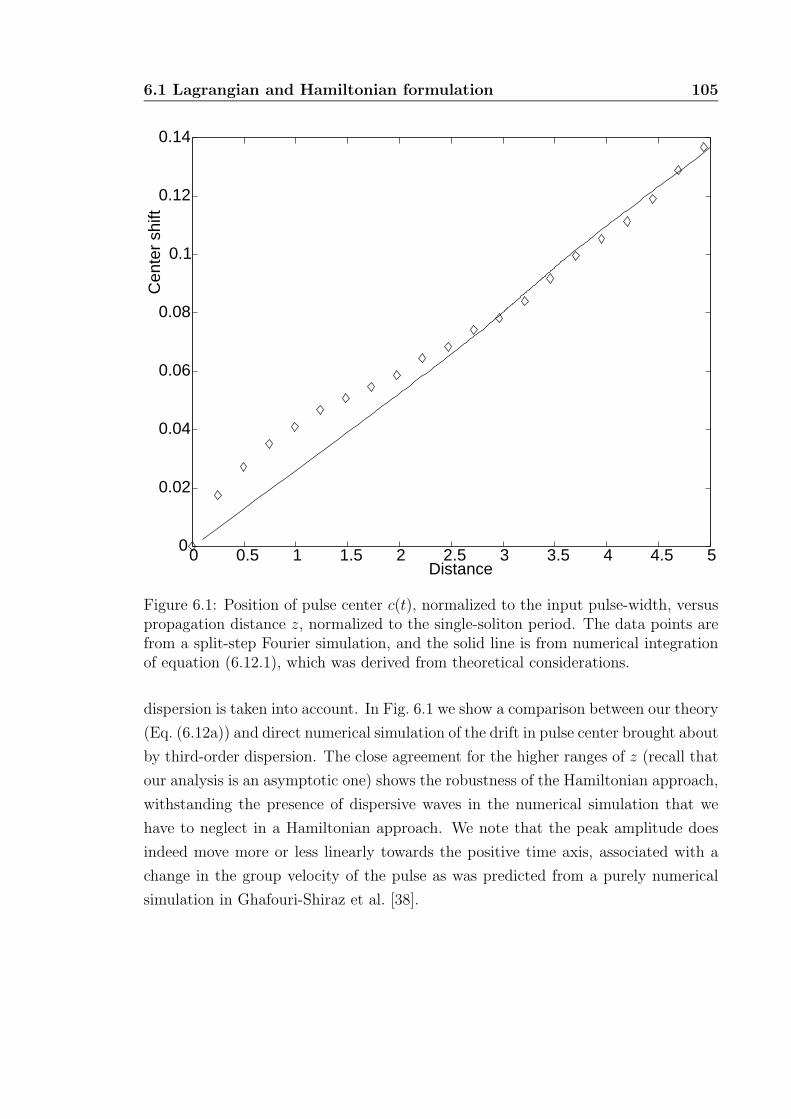
6.1 Lagrangian and Hamiltonian formulation 105
0 0.5 1 1.5 2 2.5 3 3.5 4 4.5 50
0.02
0.04
0.06
0.08
0.1
0.12
0.14
Distance
Cen
ter
shift
Figure 6.1: Position of pulse center c(t), normalized to the input pulse-width, versuspropagation distance z, normalized to the single-soliton period. The data points arefrom a split-step Fourier simulation, and the solid line is from numerical integrationof equation (6.12.1), which was derived from theoretical considerations.
dispersion is taken into account. In Fig. 6.1 we show a comparison between our theory
(Eq. (6.12a)) and direct numerical simulation of the drift in pulse center brought about
by third-order dispersion. The close agreement for the higher ranges of z (recall that
our analysis is an asymptotic one) shows the robustness of the Hamiltonian approach,
withstanding the presence of dispersive waves in the numerical simulation that we
have to neglect in a Hamiltonian approach. We note that the peak amplitude does
indeed move more or less linearly towards the positive time axis, associated with a
change in the group velocity of the pulse as was predicted from a purely numerical
simulation in Ghafouri-Shiraz et al. [38].
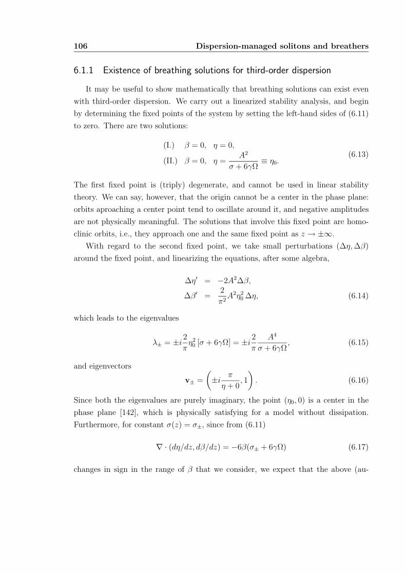
106 Dispersion-managed solitons and breathers
6.1.1 Existence of breathing solutions for third-order dispersion
It may be useful to show mathematically that breathing solutions can exist even
with third-order dispersion. We carry out a linearized stability analysis, and begin
by determining the fixed points of the system by setting the left-hand sides of (6.11)
to zero. There are two solutions:
(I.) β = 0, η = 0,
(II.) β = 0, η =A2
σ + 6γΩ≡ η0.
(6.13)
The first fixed point is (triply) degenerate, and cannot be used in linear stability
theory. We can say, however, that the origin cannot be a center in the phase plane:
orbits aproaching a center point tend to oscillate around it, and negative amplitudes
are not physically meaningful. The solutions that involve this fixed point are homo-
clinic orbits, i.e., they approach one and the same fixed point as z → ±∞.
With regard to the second fixed point, we take small perturbations (∆η, ∆β)
around the fixed point, and linearizing the equations, after some algebra,
∆η′ = −2A2∆β,
∆β′ =2
π2A2η2
0 ∆η, (6.14)
which leads to the eigenvalues
λ± = ±i2
πη2
0 [σ + 6γΩ] = ±i2
π
A4
σ + 6γΩ, (6.15)
and eigenvectors
v± =
(±i
π
η + 0, 1
). (6.16)
Since both the eigenvalues are purely imaginary, the point (η0, 0) is a center in the
phase plane [142], which is physically satisfying for a model without dissipation.
Furthermore, for constant σ(z) = σ±, since from (6.11)
∇ · (dη/dz, dβ/dz) = −6β(σ± + 6γΩ) (6.17)
changes in sign in the range of β that we consider, we expect that the above (au-
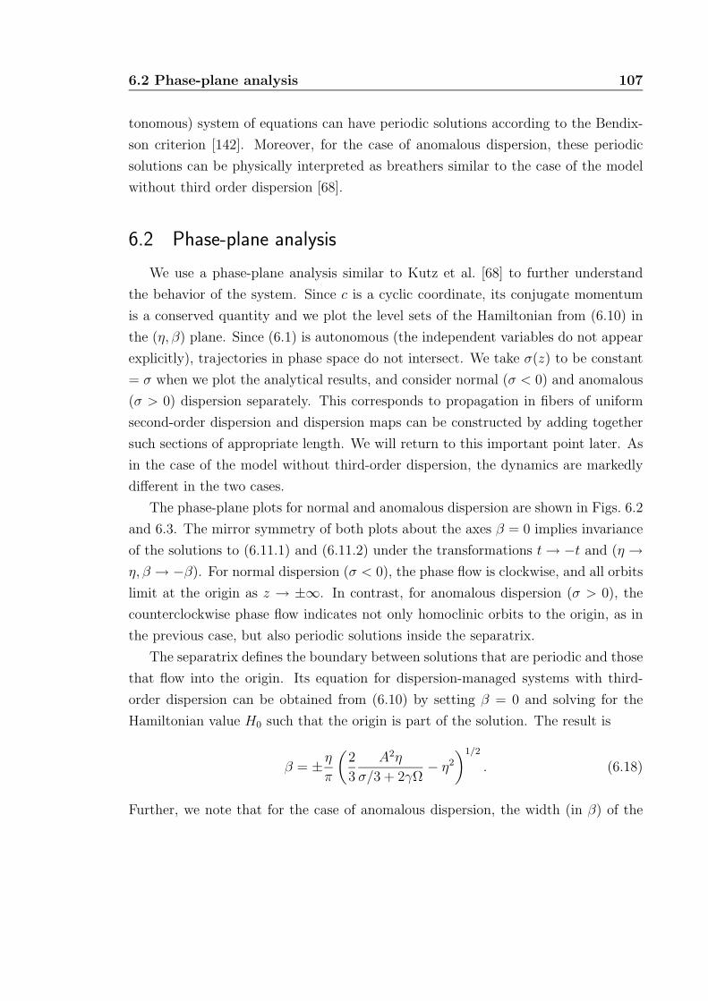
6.2 Phase-plane analysis 107
tonomous) system of equations can have periodic solutions according to the Bendix-
son criterion [142]. Moreover, for the case of anomalous dispersion, these periodic
solutions can be physically interpreted as breathers similar to the case of the model
without third order dispersion [68].
6.2 Phase-plane analysis
We use a phase-plane analysis similar to Kutz et al. [68] to further understand
the behavior of the system. Since c is a cyclic coordinate, its conjugate momentum
is a conserved quantity and we plot the level sets of the Hamiltonian from (6.10) in
the (η, β) plane. Since (6.1) is autonomous (the independent variables do not appear
explicitly), trajectories in phase space do not intersect. We take σ(z) to be constant
= σ when we plot the analytical results, and consider normal (σ < 0) and anomalous
(σ > 0) dispersion separately. This corresponds to propagation in fibers of uniform
second-order dispersion and dispersion maps can be constructed by adding together
such sections of appropriate length. We will return to this important point later. As
in the case of the model without third-order dispersion, the dynamics are markedly
different in the two cases.
The phase-plane plots for normal and anomalous dispersion are shown in Figs. 6.2
and 6.3. The mirror symmetry of both plots about the axes β = 0 implies invariance
of the solutions to (6.11.1) and (6.11.2) under the transformations t → −t and (η →η, β → −β). For normal dispersion (σ < 0), the phase flow is clockwise, and all orbits
limit at the origin as z → ±∞. In contrast, for anomalous dispersion (σ > 0), the
counterclockwise phase flow indicates not only homoclinic orbits to the origin, as in
the previous case, but also periodic solutions inside the separatrix.
The separatrix defines the boundary between solutions that are periodic and those
that flow into the origin. Its equation for dispersion-managed systems with third-
order dispersion can be obtained from (6.10) by setting β = 0 and solving for the
Hamiltonian value H0 such that the origin is part of the solution. The result is
β = ±η
π
(2
3
A2η
σ/3 + 2γΩ− η2
)1/2
. (6.18)
Further, we note that for the case of anomalous dispersion, the width (in β) of the
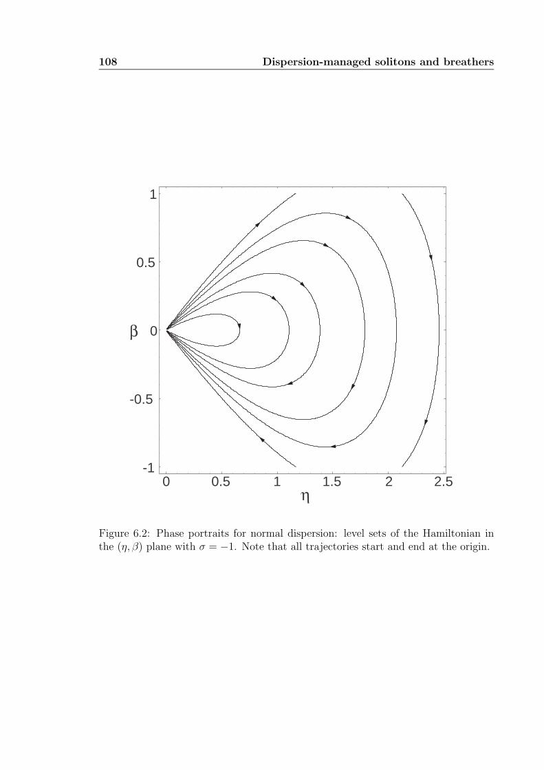
108 Dispersion-managed solitons and breathers
0 0.5 1 1.5 2 2.5-1
-0.5
0
0.5
1
β
η
Figure 6.2: Phase portraits for normal dispersion: level sets of the Hamiltonian inthe (η, β) plane with σ = −1. Note that all trajectories start and end at the origin.
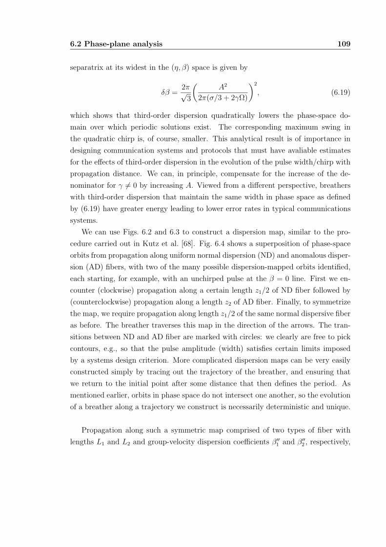
6.2 Phase-plane analysis 109
separatrix at its widest in the (η, β) space is given by
δβ =2π√
3
(A2
2π(σ/3 + 2γΩ)
)2
, (6.19)
which shows that third-order dispersion quadratically lowers the phase-space do-
main over which periodic solutions exist. The corresponding maximum swing in
the quadratic chirp is, of course, smaller. This analytical result is of importance in
designing communication systems and protocols that must have avaliable estimates
for the effects of third-order dispersion in the evolution of the pulse width/chirp with
propagation distance. We can, in principle, compensate for the increase of the de-
nominator for γ = 0 by increasing A. Viewed from a different perspective, breathers
with third-order dispersion that maintain the same width in phase space as defined
by (6.19) have greater energy leading to lower error rates in typical communications
systems.
We can use Figs. 6.2 and 6.3 to construct a dispersion map, similar to the pro-
cedure carried out in Kutz et al. [68]. Fig. 6.4 shows a superposition of phase-space
orbits from propagation along uniform normal dispersion (ND) and anomalous disper-
sion (AD) fibers, with two of the many possible dispersion-mapped orbits identified,
each starting, for example, with an unchirped pulse at the β = 0 line. First we en-
counter (clockwise) propagation along a certain length z1/2 of ND fiber followed by
(counterclockwise) propagation along a length z2 of AD fiber. Finally, to symmetrize
the map, we require propagation along length z1/2 of the same normal dispersive fiber
as before. The breather traverses this map in the direction of the arrows. The tran-
sitions between ND and AD fiber are marked with circles: we clearly are free to pick
contours, e.g., so that the pulse amplitude (width) satisfies certain limits imposed
by a systems design criterion. More complicated dispersion maps can be very easily
constructed simply by tracing out the trajectory of the breather, and ensuring that
we return to the initial point after some distance that then defines the period. As
mentioned earlier, orbits in phase space do not intersect one another, so the evolution
of a breather along a trajectory we construct is necessarily deterministic and unique.
Propagation along such a symmetric map comprised of two types of fiber with
lengths L1 and L2 and group-velocity dispersion coefficients β′′1 and β′′
2 , respectively,
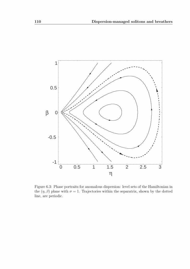
110 Dispersion-managed solitons and breathers
0 0.5 1 1.5 2 2.5 3-1
-0.5
0
0.5
1
η
β
Figure 6.3: Phase portraits for anomalous dispersion: level sets of the Hamiltonian inthe (η, β) plane with σ = 1. Trajectories within the separatrix, shown by the dottedline, are periodic.
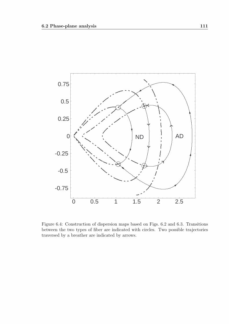
6.2 Phase-plane analysis 111
0 0.5 1 1.5 2 2.5
-0.75
-0.5
-0.25
0
0.25
0.5
0.75
ND AD
Figure 6.4: Construction of dispersion maps based on Figs. 6.2 and 6.3. Transitionsbetween the two types of fiber are indicated with circles. Two possible trajectoriestraversed by a breather are indicated by arrows.
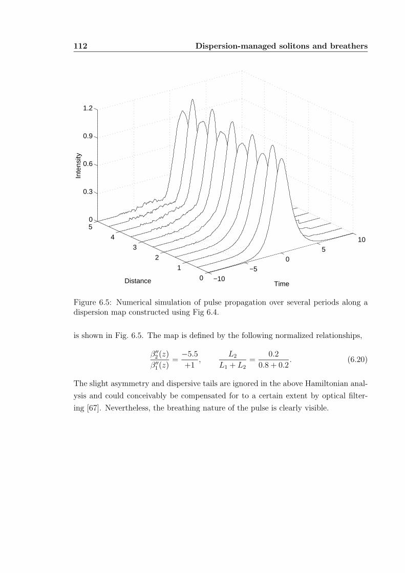
112 Dispersion-managed solitons and breathers
−10−5
05
10
0
1
2
3
4
50
0.3
0.6
0.9
1.2
TimeDistance
Inte
nsity
Figure 6.5: Numerical simulation of pulse propagation over several periods along adispersion map constructed using Fig 6.4.
is shown in Fig. 6.5. The map is defined by the following normalized relationships,
β′′2 (z)
β′′1 (z)
=−5.5
+1,
L2
L1 + L2
=0.2
0.8 + 0.2. (6.20)
The slight asymmetry and dispersive tails are ignored in the above Hamiltonian anal-
ysis and could conceivably be compensated for to a certain extent by optical filter-
ing [67]. Nevertheless, the breathing nature of the pulse is clearly visible.
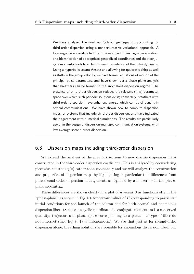
6.3 Dispersion maps including third-order dispersion 113
We have analyzed the nonlinear Schrodinger equation accounting for
third-order dispersion using a nonperturbative variational approach. A
Lagrangian was constructed from the modified Euler-Lagrange equation,
and identification of appropriate generalized coordinates and their conju-
gate momenta leads to a Hamiltonian formulation of the pulse dynamics.
Using a hyperbolic secant Ansatz and allowing for quadratic chirp as well
as shifts in the group velocity, we have formed equations of motion of the
principal pulse parameters, and have shown via a phase-plane analysis
that breathers can be formed in the anomalous dispersion regime. The
presence of third-order dispersion reduces the relevant (η, β) parameter
space over which such periodic solutions exist; conversely, breathers with
third-order dispersion have enhanced energy which can be of benefit in
optical communications. We have shown how to compute dispersion
maps for systems that include third-order dispersion, and have indicated
their agreement with numerical simulations. The results are particularly
useful in the design of dispersion-managed communication systems, with
low average second-order dispersion.
6.3 Dispersion maps including third-order dispersion
We extend the analysis of the previous sections to now discuss dispersion maps
constructed in the third-order dispersion coefficient. This is analyzed by coonsidering
piecewise constant γ(z) rather than constant γ and we will analyze the construction
and properties of dispersion maps by highlighting in particular the differences from
pure second-order dispersion management, as signified by a nonzero γ in the phase-
plane separatrix.
These differences are shown clearly in a plot of η versus β as functions of z in the
“phase-plane” as shown in Fig. 6.6 for certain values of H corresponding to particular
initial conditions for the launch of the soliton and for both normal and anomalous
dispersion fiber. (Since c is a cyclic coordinate, its conjugate momentum is a conserved
quantity; trajectories in phase space corresponding to a particular type of fiber do
not intersect since Eq. (6.1) is autonomous.) We see that just as for second-order
dispersion alone, breathing solutions are possible for anomalous dispersion fiber, but
114 Dispersion-managed solitons and breathers
the countours are scaled nonlinearly in the phase plane. In this regime, the separatrix
defines the boundary between solutions that are periodic and those that flow into the
origin.
1 2
-0.75
-0.5
-0.25
0.25
0.5
0.75
ND
AD
ηβ
δβ/2
δη
Figure 6.6: Change in the trajectory of a breather from second-order dispersion alone(dotted line) to combined second- and third-order dispersion (solid line). Normaldispersion (ND) fibers are traversed clockwise and anomalous dispersion (AD) fibersanticlockwise. The δβ and δη in this figure do not refer to the separatrix but to ageneric trajectory as shown.
From the separatrix Eq. (6.18), we can derive certain phase-space widths of inter-
est. At its widest along the β coordinate, the separatrix width is obtained by solving
6.3 Dispersion maps including third-order dispersion 115
dβ/dη = 0 for η = η and then finding δβ = 2β(η), which yields
δβ =2π√
3
(A2
2π(σ/3 + 2γΩ)
)2
, (6.21)
where η = A2/[2(σ/3 + 2γΩ)]. Similarly, stipulating that dβ/dη becomes infinite for
finite η leads to the maximum value of η, since (η, β) = (0, 0) is trivially part of the
separatrix Eq. (6.18),
δη =2π√
3
A2
σ/3 + 2γΩ. (6.22)
We see that the effects of nonzero γ are different along the two coordinates. Con-
sider the case where σ and γ have the same sign: whereas the separatrix contracts
linearly along the η-axis, it contracts quadratically along the β axis. The role of TOD
is therefore nontrivial and cannot be simply “cancelled” by chosing an appropriately
scaled-up contour relative to the separatrix for second-order dispersion alone. While
this conclusion is intuitive, the precise argument is most meaningful and precise when
approached from the Hamiltonian formalism described here.
Since we know a Hamiltonian describing the evolution of a breather along sections
of normal or anomalous dispersive fiber, we can ask if the effect of TOD in shrinking
the contours can be compensated for by varying the TOD coefficient γ in sign between
the two sections of fiber that comprise a dispersion map in the second-order dispersion
coefficient σ. We note that TOD also results in a translation of the contours, i.e., of
the linearized center in the phase plane [90] but that is of less importance in this
context, since a dispersion map may always be constructed in theory by selecting
sufficiently outlying contours.
Contours in phase space aside from the separatrix are parametrized by a particular
value H∗ of the Hamiltonian (6.10). For any given H∗, we can find the greatest extent
of the contour along the η axis (with β = 0). Since the equation of motion (6.11) for
β is symmetric in β → −β, this point can be found by determining that η ≡ ζ for
which dβ/dη goes to infinity at finite η. Alternatively, we can set β(η) = 0 and solve
for the greatest η. The results are identical and we obtain after some algebra that
116 Dispersion-managed solitons and breathers
the maximum value of η is
ζ =A2
σ + 6γΩ
1 ∓
√1 −
(σ + 6γΩ
A2
)2 [3H∗
2A2(σ + 6γΩ)+ Ω2
(1 + 2
σ
σ + 6γΩ
)] ,
(6.23)
where the minus sign corresponds to a section of fiber with normal dispersion (σ < 0)
and the plus sign for anomalous dispersion (σ > 0).
The simplest dispersion maps involve two sections of fiber with σ taking on op-
posite signs, i.e., σ(z) = ∓σ for normal and anomalous dispersion fiber, respectively.
We now ask if it is possible to design a dispersion map with TOD to maintain the
same separation between the two contours in phase space along the η axis. We use
a subscript N or A on ζ to indicate normal or anomalous dispersion fiber, and a
superscript ζ(0) for second-order dispersion alone and ζ(1) for a dispersion map that
includes TOD. Stated mathematically, we seek the conditions under which
∆ζN ≡ ζ(0)N − ζ
(1)N = ζ
(0)A − ζ
(1)A ≡ ∆ζA, (6.24)
where the normal dispersion contour is selected by a Hamiltonian value H∗N and the
anomalous dispersion contour by H∗A.
From (6.23), we have
ζ(0)N =
A2
−σ
[1 −
√1 −
( σ
A2
)2[
3H∗N
2A2(−σ)+ 3Ω2
]], (6.25)
ζ(1)N =
A2
−σ + 6γNΩ
[1 −
√1 −
(−σ + 6γNΩ
A2
)2 [3H∗
N
2A2(−σ + 6γNΩ)+ Ω2
(1 + 2
−σ
−σ + 6γNΩ
)]],
and similarly for ζ(0)A and ζ
(1)A with the replacements γN → γA, −σ → σ and the
appropriate sign from (6.23).
6.3 Dispersion maps including third-order dispersion 117
Therefore,
∆ζN =
[A2
−σ− A2
−σ + 6γNΩ
]+
A2
σ
√1 −
( σ
A2
)2[−3H∗
N
2A2σ+ 3Ω2
](6.26)
− A2
σ − 6γNΩ
√1 −
(σ − 6γNΩ
A2
)2 [ −3H∗N
2A2(σ − 6γNΩ)+ Ω2
(1 +
2σ
σ − 6γNΩ
)]
∆ζA =
[A2
σ− A2
σ + 6γAΩ
]+
A2
σ
√1 −
( σ
A2
)2[
3H∗A
2A2σ+ 3Ω2
](6.27)
− A2
σ + 6γAΩ
√1 −
(σ + 6γAΩ
A2
)2 [3H∗
A
2A2(σ + 6γAΩ)+ Ω2
(1 +
2σ
σ + 6γAΩ
)] .
Substituting the above expressions into (6.24) yields a complicated equation,
which can be simplified by noting that if for four rationals x +√
y = a +√
b, then
x = a and y = b unless y and b are the squares of rationals. Inspection of (6.26)
and (6.27) shows that the general condition holds, except possibly for one particular
set of values of H∗, which is unlikely to be the exact H∗ that constructs a satisfactory
dispersion map. In any case, it is not practical to impose the Hamiltonian energy to
exactly equal a particular irrational number. Consequently, we can split the condition
∆ζN = ∆ζA into a pair of simultaneous equations, one for the rational part free from
radicals (in this case, the square root) and the other involving (only) radicals (also
known as a “surd”). The first equation of this pair [see (6.26) and (6.27)] then leads
to the requirement1
−σ− 1
−σ + 6γNΩ=
1
σ− 1
σ + 6γAΩ, (6.28)
which after a little algebra simplifies to
1
6Ω
(1
γN
− 1
γA
)=
2
σ. (6.29)
Next, the second terms of (6.26) and (6.27) (involving the radical) can be seen to be
identical for both ∆ζN and ∆ζA if
γN = −γA (6.30)
118 Dispersion-managed solitons and breathers
and we choose contours (i.e., H∗) appropriately. Combining (6.29) and (6.30) yields
the simple condition
σ = 6γΩ, (6.31)
where γN = −γA ≡ γ just as σA = −σN ≡ σ. But σN + 6γNΩ = 0, which sets the
denominator of (6.23) to zero—therefore, the result (6.31) is not a physically mean-
ingful one. This shows that third-order dispersion fundamentally modifies even the
the swing in pulse amplitude and since this is a typical design criterion in dispersion-
managed systems, it is important to design dispersion maps explicitly taking the
effects of γ into account. An example of such a map was discussed elsewhere [90].
This analysis of dispersion-mapped TOD solitons can considerably help the search
for effective ways to compensate for dispersion-slope [3] mismatch in dispersion-
mapped systems [148]. In systems that use nonlinear breathing pulse shapes (en-
velopes), we can explicitly use the dispersion-slope mismatch between different sec-
tions of nonlinear fiber to pick appropriate contours in the phase space. The periodic
dispersion map thereby constructed has breathing solutions that inherently utilize the
different third-order dispersion coefficients encountered along the propagation chan-
nel and the residual mismatch is then of fourth order in chromatic dispersion and
consequently much weaker. The emphasis is now on utilizing third-order dispersion
constructively rather than trying to completely get rid of the effect. Of course, the
Hamiltonian analysis is valid only within certain regimes, and TOD dispersion maps
can be used to utilize the residual dispersion-slope mismatch after reasonably simple
dispersion-slope mismatch compensation schemes have been applied—this will ease
the burden on the latter functionality.
We have shown that the presence of third-order dispersion (TOD)
scales the representative periodic orbit in phase-space—the separatrix—
differently along the two coordinates η and β. For both normal dis-
persion and anomalous dispersion fiber, we have quantified the changes
in the variations of the amplitude (or pulse width) and the quadratic
chirp of the pulse envelope. It is clear that TOD modifies the orbits
in phase-space nontrivially; we have also shown that it is necessary to
explicitly consider TOD even with simpler design constraints, such as
the maximum periodic change in pulse amplitude.
Chapter 7
Multilevel communications in nonlinear fibers
Oh.We have reached the crux of the matter.
The argument that the location of the pole in the quark propagator is anobservable quantity rests upon the assumption that there is no confinement.
Those who look for confinement in the singularities of the quarkpropagator are like the man who settled in Casablanca for the waters.
They have been misinformed.
—S. Coleman, Aspects of Symmetry, Cambridge, 1985.
As we have seen in Chapter 6, a physically intuitive framework for understanding
and predicting the nonlinear evolution of optical pulses (applicable to non-integrable
systems) is the variational characterization of breather dynamics [100, 7] based on
a Lagrangian functional and an appropriate Ansatz for the pulse envelope. The
resulting equations of motion of the pulse parameters, Eqs. (6.11) and (6.12), can be
represented in the phase-plane, simplifying the construction of appropriate dispersion
maps of the group-velocity dispersion (GVD) coefficient [68].
We have proposed a multilevel optical communications scheme using nonlinear
pulses that can substantially increase the bitrate of current signalling formats, since
the advantages are essentially independent of wavelength- and time-division multi-
plexing. This scheme is simply not possible with conventional linear transmission
formats that ignore the Kerr effect in optical fibers, and it relies extensively on un-
derstanding the implications of the equations of motion of the pulse parameters. The
context of this proposal is introduced in Section 7.1, and an overview is presented in
Section 7.3. The remainder of this chapter is mainly concerned with the technical
details of implementing a practical system in the presence of amplifier noise. Quan-
titative estimates of the benefit of this scheme using realistic estimates of the various
119
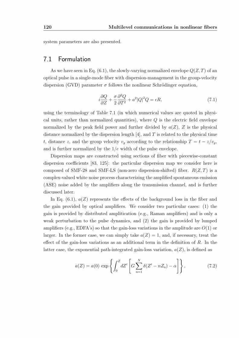
120 Multilevel communications in nonlinear fibers
system parameters are also presented.
7.1 Formulation
As we have seen in Eq. (6.1), the slowly-varying normalized envelope Q(Z, T ) of an
optical pulse in a single-mode fiber with dispersion-management in the group-velocity
dispersion (GVD) parameter σ follows the nonlinear Schrodinger equation,
i∂Q
∂Z+
σ
2
∂2Q
∂T 2+ a2|Q|2Q = εR, (7.1)
using the terminology of Table 7.1 (in which numerical values are quoted in physi-
cal units, rather than normalized quantities), where Q is the electric field envelope
normalized by the peak field power and further divided by a(Z), Z is the physical
distance normalized by the dispersion length [4], and T is related to the physical time
t, distance z, and the group velocity vg according to the relationship T = t − z/vg,
and is further normalized by the 1/e width of the pulse envelope.
Dispersion maps are constructed using sections of fiber with piecewise-constant
dispersion coefficients [83, 125]: the particular dispersion map we consider here is
composed of SMF-28 and SMF-LS (non-zero dispersion-shifted) fiber. R(Z, T ) is a
complex-valued white noise process characterizing the amplified spontaneous emission
(ASE) noise added by the amplifiers along the transmission channel, and is further
discussed later.
In Eq. (6.1), a(Z) represents the effects of the background loss in the fiber and
the gain provided by optical amplifiers. We consider two particular cases: (1) the
gain is provided by distributed amplitication (e.g., Raman amplifiers) and is only a
weak perturbation to the pulse dynamics, and (2) the gain is provided by lumped
amplifiers (e.g., EDFA’s) so that the gain-loss variations in the amplitude are O(1) or
larger. In the former case, we can simply take a(Z) = 1, and, if necessary, treat the
effect of the gain-loss variations as an additional term in the definition of R. In the
latter case, the exponential path-integrated gain-loss variation, a(Z), is defined as
a(Z) = a(0) exp
∫ Z
0
dZ ′[G
N∑n=1
δ(Z ′ − nZa) − α
], (7.2)
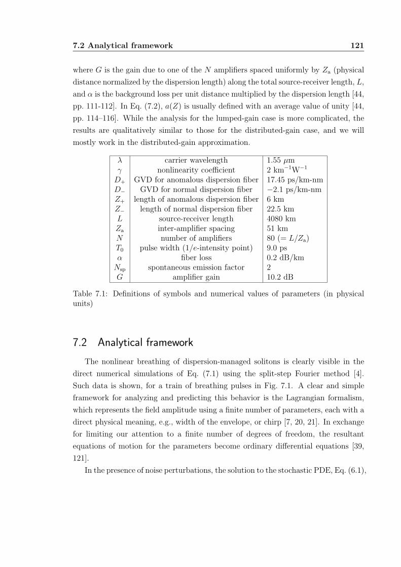
7.2 Analytical framework 121
where G is the gain due to one of the N amplifiers spaced uniformly by Za (physical
distance normalized by the dispersion length) along the total source-receiver length, L,
and α is the background loss per unit distance multiplied by the dispersion length [44,
pp. 111-112]. In Eq. (7.2), a(Z) is usually defined with an average value of unity [44,
pp. 114–116]. While the analysis for the lumped-gain case is more complicated, the
results are qualitatively similar to those for the distributed-gain case, and we will
mostly work in the distributed-gain approximation.
λ carrier wavelength 1.55 µmγ nonlinearity coefficient 2 km−1W−1
D+ GVD for anomalous dispersion fiber 17.45 ps/km-nmD− GVD for normal dispersion fiber −2.1 ps/km-nmZ+ length of anomalous dispersion fiber 6 kmZ− length of normal dispersion fiber 22.5 kmL source-receiver length 4080 kmZa inter-amplifier spacing 51 kmN number of amplifiers 80 (= L/Za)T0 pulse width (1/e-intensity point) 9.0 psα fiber loss 0.2 dB/km
Nsp spontaneous emission factor 2G amplifier gain 10.2 dB
Table 7.1: Definitions of symbols and numerical values of parameters (in physicalunits)
7.2 Analytical framework
The nonlinear breathing of dispersion-managed solitons is clearly visible in the
direct numerical simulations of Eq. (7.1) using the split-step Fourier method [4].
Such data is shown, for a train of breathing pulses in Fig. 7.1. A clear and simple
framework for analyzing and predicting this behavior is the Lagrangian formalism,
which represents the field amplitude using a finite number of parameters, each with a
direct physical meaning, e.g., width of the envelope, or chirp [7, 20, 21]. In exchange
for limiting our attention to a finite number of degrees of freedom, the resultant
equations of motion for the parameters become ordinary differential equations [39,
121].
In the presence of noise perturbations, the solution to the stochastic PDE, Eq. (6.1),
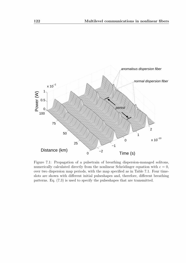
122 Multilevel communications in nonlinear fibers
−2
−1
0
1
2
x 10−10
0
25
50
75
1000
0.5
1
x 10−2
Time (s)Distance (km)
Pow
er (
W)
normal dispersion fiber
anomalous dispersion fiber
period
Figure 7.1: Propagation of a pulsetrain of breathing dispersion-managed solitons,numerically calculated directly from the nonlinear Schrodinger equation with ε = 0,over two dispersion map periods, with the map specified as in Table 7.1. Four time-slots are shown with different initial pulseshapes and, therefore, different breathingpatterns. Eq. (7.3) is used to specify the pulseshapes that are transmitted.
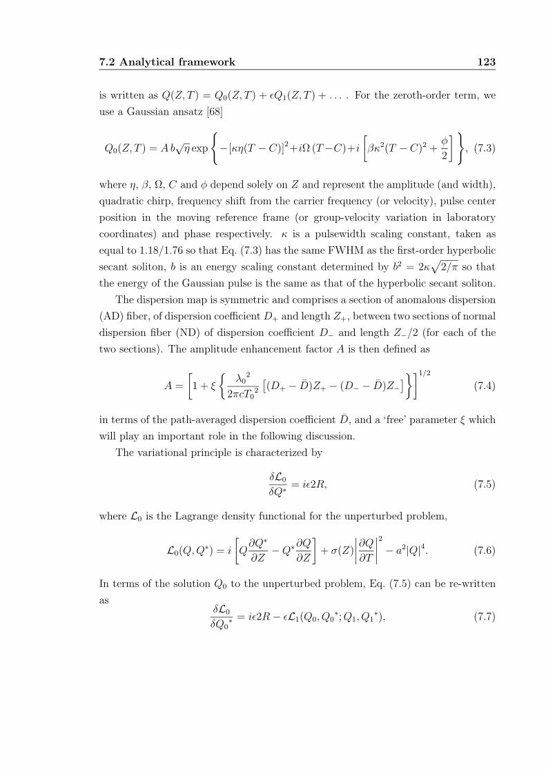
7.2 Analytical framework 123
is written as Q(Z, T ) = Q0(Z, T ) + εQ1(Z, T ) + . . . . For the zeroth-order term, we
use a Gaussian ansatz [68]
Q0(Z, T ) = Ab√
η exp
−[κη(T − C)]2+iΩ (T−C)+i
[βκ2(T − C)2 +
φ
2
], (7.3)
where η, β, Ω, C and φ depend solely on Z and represent the amplitude (and width),
quadratic chirp, frequency shift from the carrier frequency (or velocity), pulse center
position in the moving reference frame (or group-velocity variation in laboratory
coordinates) and phase respectively. κ is a pulsewidth scaling constant, taken as
equal to 1.18/1.76 so that Eq. (7.3) has the same FWHM as the first-order hyperbolic
secant soliton, b is an energy scaling constant determined by b2 = 2κ√
2/π so that
the energy of the Gaussian pulse is the same as that of the hyperbolic secant soliton.
The dispersion map is symmetric and comprises a section of anomalous dispersion
(AD) fiber, of dispersion coefficient D+ and length Z+, between two sections of normal
dispersion fiber (ND) of dispersion coefficient D− and length Z−/2 (for each of the
two sections). The amplitude enhancement factor A is then defined as
A =
[1 + ξ
λ0
2
2πcT02
[(D+ − D)Z+ − (D− − D)Z−
]]1/2
(7.4)
in terms of the path-averaged dispersion coefficient D, and a ‘free’ parameter ξ which
will play an important role in the following discussion.
The variational principle is characterized by
δL0
δQ∗ = iε2R, (7.5)
where L0 is the Lagrange density functional for the unperturbed problem,
L0(Q,Q∗) = i
[Q
∂Q∗
∂Z− Q∗∂Q
∂Z
]+ σ(Z)
∣∣∣∣∂Q
∂T
∣∣∣∣2
− a2|Q|4. (7.6)
In terms of the solution Q0 to the unperturbed problem, Eq. (7.5) can be re-written
asδL0
δQ0∗ = iε2R − εL1(Q0, Q0
∗; Q1, Q1∗), (7.7)
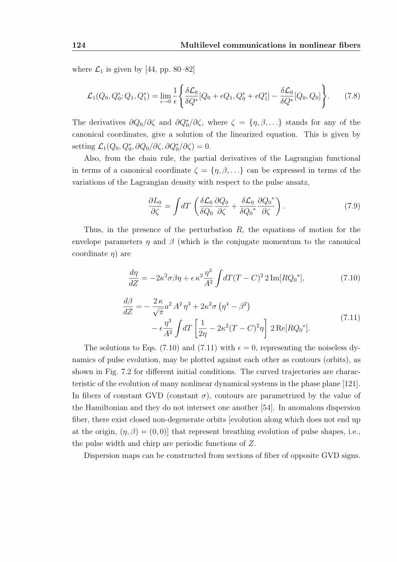
124 Multilevel communications in nonlinear fibers
where L1 is given by [44, pp. 80–82]
L1(Q0, Q∗0; Q1, Q
∗1) = lim
ε→0
1
ε
δL0
δQ∗ [Q0 + εQ1, Q∗0 + εQ∗
1] −δL0
δQ∗ [Q0, Q0]
. (7.8)
The derivatives ∂Q0/∂ζ and ∂Q∗0/∂ζ, where ζ = η, β, . . . stands for any of the
canonical coordinates, give a solution of the linearized equation. This is given by
setting L1(Q0, Q∗0, ∂Q0/∂ζ, ∂Q∗
0/∂ζ) = 0.
Also, from the chain rule, the partial derivatives of the Lagrangian functional
in terms of a canonical coordinate ζ = η, β, . . . can be expressed in terms of the
variations of the Lagrangian density with respect to the pulse ansatz,
∂L0
∂ζ=
∫dT
(δL0
δQ0
∂Q0
∂ζ+
δL0
δQ0∗∂Q0
∗
∂ζ
). (7.9)
Thus, in the presence of the perturbation R, the equations of motion for the
envelope parameters η and β (which is the conjugate momentum to the canonical
coordinate η) are
dη
dZ= −2κ2σβη + ε κ2 η3
A2
∫dT (T − C)2 2 Im[RQ0
∗], (7.10)
dβ
dZ= − 2 κ√
πa2 A2 η3 + 2κ2σ
(η4 − β2
)− ε
η3
A2
∫dT
[1
2η− 2κ2(T − C)2η
]2 Re[RQ0
∗].(7.11)
The solutions to Eqs. (7.10) and (7.11) with ε = 0, representing the noiseless dy-
namics of pulse evolution, may be plotted against each other as contours (orbits), as
shown in Fig. 7.2 for different initial conditions. The curved trajectories are charac-
teristic of the evolution of many nonlinear dynamical systems in the phase plane [121].
In fibers of constant GVD (constant σ), contours are parametrized by the value of
the Hamiltonian and they do not intersect one another [54]. In anomalous dispersion
fiber, there exist closed non-degenerate orbits [evolution along which does not end up
at the origin, (η, β) = (0, 0)] that represent breathing evolution of pulse shapes, i.e.,
the pulse width and chirp are periodic functions of Z.
Dispersion maps can be constructed from sections of fiber of opposite GVD signs.
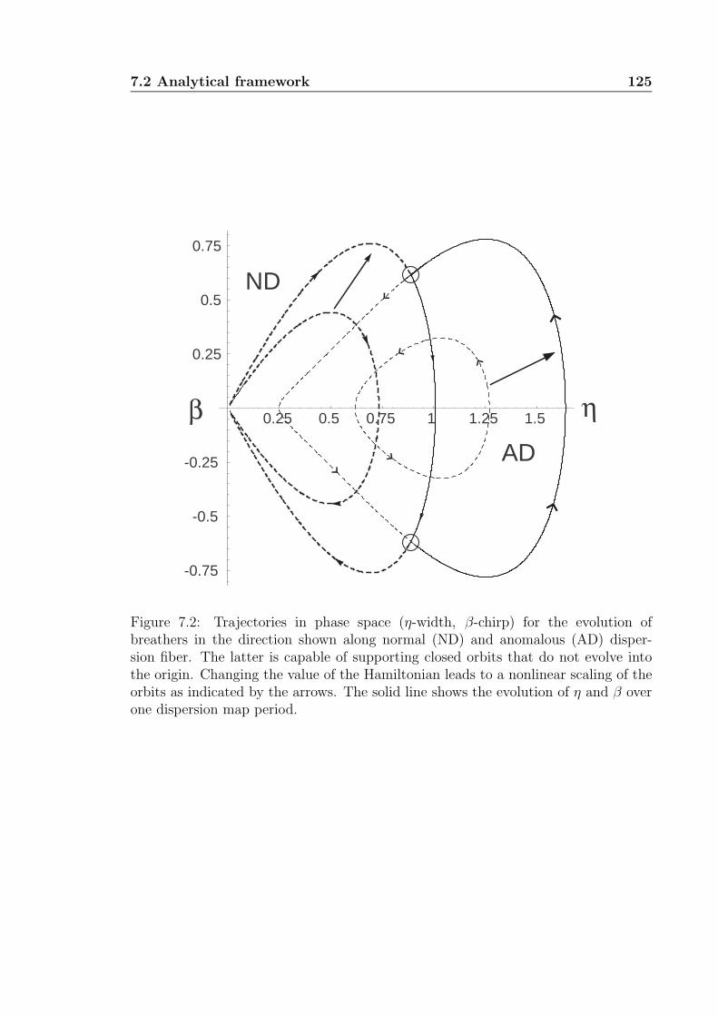
7.2 Analytical framework 125
0.25 0.5 0.75 1 1.25 1.5
-0.75
-0.5
-0.25
0.25
0.5
0.75
ND
AD
β η
Figure 7.2: Trajectories in phase space (η-width, β-chirp) for the evolution ofbreathers in the direction shown along normal (ND) and anomalous (AD) disper-sion fiber. The latter is capable of supporting closed orbits that do not evolve intothe origin. Changing the value of the Hamiltonian leads to a nonlinear scaling of theorbits as indicated by the arrows. The solid line shows the evolution of η and β overone dispersion map period.
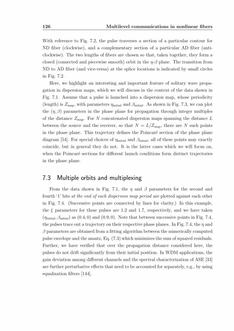
126 Multilevel communications in nonlinear fibers
With reference to Fig. 7.2, the pulse traverses a section of a particular contour for
ND fiber (clockwise), and a complementary section of a particular AD fiber (anti-
clockwise). The two lengths of fibers are chosen so that, taken together, they form a
closed (connected and piecewise smooth) orbit in the η-β plane. The transition from
ND to AD fiber (and vice-versa) at the splice locations is indicated by small circles
in Fig. 7.2.
Here, we highlight an interesting and important feature of solitary wave propa-
gation in dispersion maps, which we will discuss in the context of the data shown in
Fig. 7.1. Assume that a pulse is launched into a dispersion map, whose periodicity
(length) is Zmap, with parameters ηinitial and βinitial. As shown in Fig. 7.3, we can plot
the (η, β) parameters in the phase plane for propagation through integer multiples
of the distance Zmap. For N concatenated dispersion maps spanning the distance L
between the source and the receiver, so that N = L/Zmap, there are N such points
in the phase plane. This trajectory defines the Poincare section of the phase plane
diagram [54]. For special choices of ηinitial and βinitial, all of these points may exactly
coincide, but in general they do not. It is the latter cases which we will focus on,
when the Poincare sections for different launch conditions form distinct trajectories
in the phase plane.
7.3 Multiple orbits and multiplexing
From the data shown in Fig. 7.1, the η and β parameters for the second and
fourth ‘1’ bits at the end of each dispersion map period are plotted against each other
in Fig. 7.4. (Successive points are connected by lines for clarity.) In this example,
the ξ parameters for these pulses are 1.2 and 1.7, respectively, and we have taken
(ηinitial, βinitial) as (0.4, 0) and (0.9, 0). Note that between successive points in Fig. 7.4,
the pulses trace out a trajectory on their respective phase planes. In Fig. 7.4, the η and
β parameters are obtained from a fitting algorithm between the numerically computed
pulse envelope and the ansatz, Eq. (7.3) which minimizes the sum of squared residuals.
Further, we have verified that over the propagation distance considered here, the
pulses do not drift significantly from their initial position. In WDM applications, the
gain deviation among different channels and the spectral characterization of ASE [33]
are further perturbative effects that need to be accounted for separately, e.g., by using
equalization filters [144].
7.3 Multiple orbits and multiplexing 127
−2
−1
0
1
2
x 10−10
320
340
360
380
400
0
0.5
1x 10
−2
Time(s) Distance (km)
Pow
er (
W)
0.7 0.8 0.9 1 1.1 1.2 1.3 1.4−0.2
0
0.2
0.4
0.6
0.8
1
1.2
1.4
η
β
Figure 7.3: The correspondence between the numerically calculated temporal profileand the fitted paramters in the phase-plane, emphasizing that points in the phaseplane are plotted at the end of each dispersion map period. Three such points arehighlighted in this representation. Each of the points shown in Fig. 7.4 is obtainedin this manner.
As Fig. 7.4 shows, there can exist more than one closed orbit in the phase-plane
(for clarity, we have shown only two). The multiplexing scheme works as follows: the
source (laser+modulator) launches a pulse with a particular combination of amplitude
(width), η, and chirp, β to place a particular pulse onto a selected trajectory, i.e.,
by choosing an initial value for η = ηinitial and for β = βinitial, we select the unique
contour that the pulse follows as it propagates. Small unpredicted variations in the
initial parameters will select an adjacent contour, but this is not of much concern if
the separation between the contours assigned to different codes is chosen to be large
enough.
Different contours are assigned to the various alphabets of a multi-level code. The
cardinality of the alphabet depends on the complexity of the receivers. For current
receiver technology, it is practical to require an unchirped pulse be received at the
detector. In this case, there are two allowed pairs, (ηfinal, 0), for each orbit, and the
two orbits shown in Fig. 7.4implement a four-symbol multiplexing scheme. The single
channel bit rate (1/inter-pulse separation) is multiplied by four.
Components of the technology needed to implement such a multiplexing scheme
have already been demonstrated. For the transmitter, a simple and practical way of
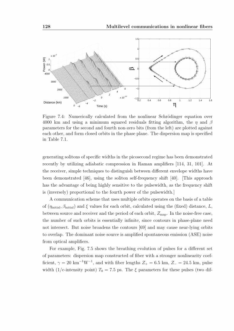
128 Multilevel communications in nonlinear fibers
−6−4
−20
24
6
x 10−10
0
1000
2000
3000
4000
0
0.5
1x 10
−2
Time (s)Distance (km)
Po
we
r (W
)
0.2 0.4 0.6 0.8 1 1.2 1.4 1.6−1.5
−1
−0.5
0
0.5
1
1.5
η
β
Figure 7.4: Numerically calculated from the nonlinear Schrodinger equation over4000 km and using a minimum squared residuals fitting algorithm, the η and βparameters for the second and fourth non-zero bits (from the left) are plotted againsteach other, and form closed orbits in the phase plane. The dispersion map is specifiedin Table 7.1.
generating solitons of specific widths in the picosecond regime has been demonstrated
recently by utilizing adiabatic compression in Raman amplifiers [114, 31, 101]. At
the receiver, simple techniques to distinguish between different envelope widths have
been demonstrated [46], using the soliton self-frequency shift [40]. [This approach
has the advantage of being highly sensitive to the pulsewidth, as the frequency shift
is (inversely) proportional to the fourth power of the pulsewidth.]
A communication scheme that uses multiple orbits operates on the basis of a table
of (ηinitial, βinitial) and ξ values for each orbit, calculated using the (fixed) distance, L,
between source and receiver and the period of each orbit, Zmap. In the noise-free case,
the number of such orbits is essentially infinite, since contours in phase-plane need
not intersect. But noise broadens the contours [69] and may cause near-lying orbits
to overlap. The dominant noise source is amplified spontaneous emission (ASE) noise
from optical amplifiers.
For example, Fig. 7.5 shows the breathing evolution of pulses for a different set
of parameters: dispersion map constructed of fiber with a stronger nonlinearity coef-
ficient, γ = 20 km−1W−1, and with fiber lengths Z+ = 6.5 km, Z− = 24.5 km, pulse
width (1/e-intensity point) T0 = 7.5 ps. The ξ parameters for these pulses (two dif-
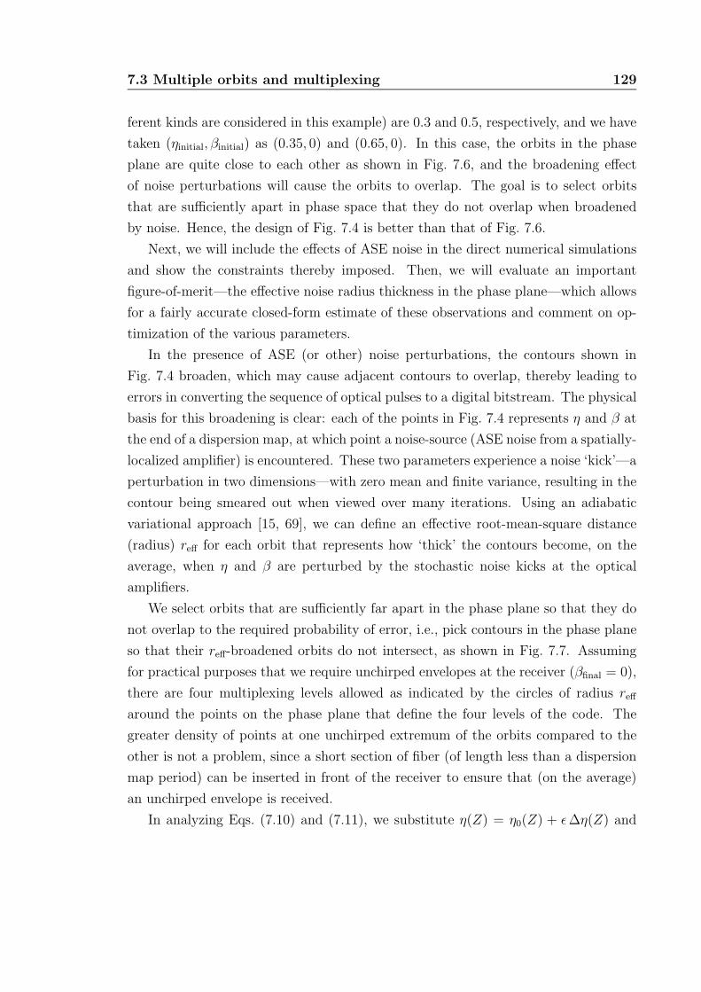
7.3 Multiple orbits and multiplexing 129
ferent kinds are considered in this example) are 0.3 and 0.5, respectively, and we have
taken (ηinitial, βinitial) as (0.35, 0) and (0.65, 0). In this case, the orbits in the phase
plane are quite close to each other as shown in Fig. 7.6, and the broadening effect
of noise perturbations will cause the orbits to overlap. The goal is to select orbits
that are sufficiently apart in phase space that they do not overlap when broadened
by noise. Hence, the design of Fig. 7.4 is better than that of Fig. 7.6.
Next, we will include the effects of ASE noise in the direct numerical simulations
and show the constraints thereby imposed. Then, we will evaluate an important
figure-of-merit—the effective noise radius thickness in the phase plane—which allows
for a fairly accurate closed-form estimate of these observations and comment on op-
timization of the various parameters.
In the presence of ASE (or other) noise perturbations, the contours shown in
Fig. 7.4 broaden, which may cause adjacent contours to overlap, thereby leading to
errors in converting the sequence of optical pulses to a digital bitstream. The physical
basis for this broadening is clear: each of the points in Fig. 7.4 represents η and β at
the end of a dispersion map, at which point a noise-source (ASE noise from a spatially-
localized amplifier) is encountered. These two parameters experience a noise ‘kick’—a
perturbation in two dimensions—with zero mean and finite variance, resulting in the
contour being smeared out when viewed over many iterations. Using an adiabatic
variational approach [15, 69], we can define an effective root-mean-square distance
(radius) reff for each orbit that represents how ‘thick’ the contours become, on the
average, when η and β are perturbed by the stochastic noise kicks at the optical
amplifiers.
We select orbits that are sufficiently far apart in the phase plane so that they do
not overlap to the required probability of error, i.e., pick contours in the phase plane
so that their reff-broadened orbits do not intersect, as shown in Fig. 7.7. Assuming
for practical purposes that we require unchirped envelopes at the receiver (βfinal = 0),
there are four multiplexing levels allowed as indicated by the circles of radius reff
around the points on the phase plane that define the four levels of the code. The
greater density of points at one unchirped extremum of the orbits compared to the
other is not a problem, since a short section of fiber (of length less than a dispersion
map period) can be inserted in front of the receiver to ensure that (on the average)
an unchirped envelope is received.
In analyzing Eqs. (7.10) and (7.11), we substitute η(Z) = η0(Z) + ε ∆η(Z) and
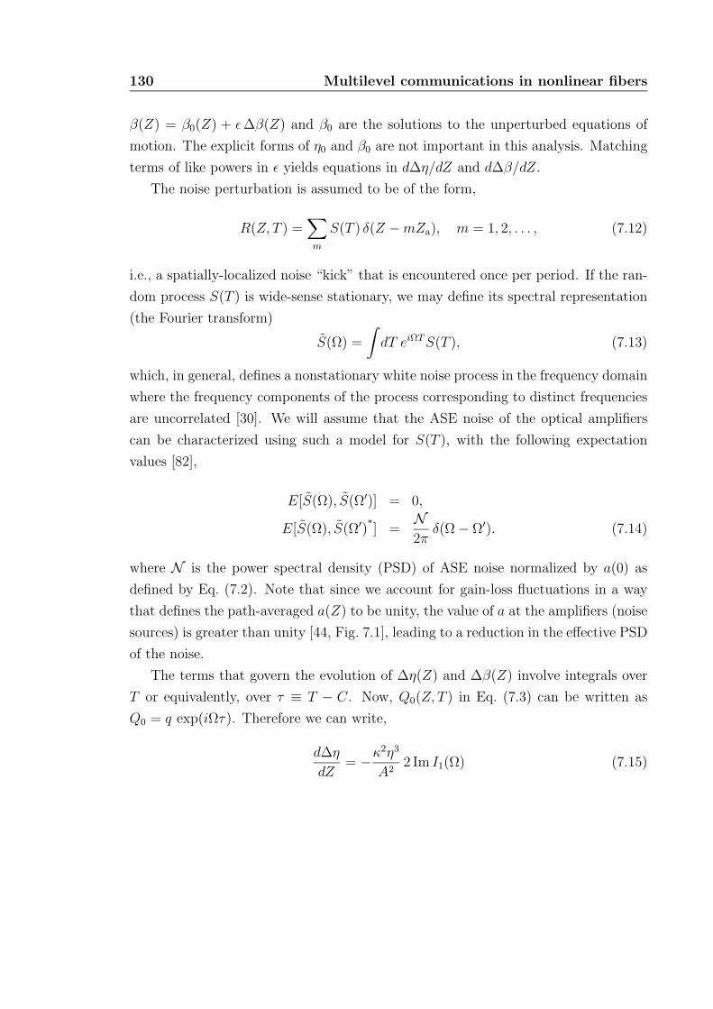
130 Multilevel communications in nonlinear fibers
β(Z) = β0(Z) + ε ∆β(Z) and β0 are the solutions to the unperturbed equations of
motion. The explicit forms of η0 and β0 are not important in this analysis. Matching
terms of like powers in ε yields equations in d∆η/dZ and d∆β/dZ.
The noise perturbation is assumed to be of the form,
R(Z, T ) =∑m
S(T ) δ(Z − mZa), m = 1, 2, . . . , (7.12)
i.e., a spatially-localized noise “kick” that is encountered once per period. If the ran-
dom process S(T ) is wide-sense stationary, we may define its spectral representation
(the Fourier transform)
S(Ω) =
∫dT eiΩT S(T ), (7.13)
which, in general, defines a nonstationary white noise process in the frequency domain
where the frequency components of the process corresponding to distinct frequencies
are uncorrelated [30]. We will assume that the ASE noise of the optical amplifiers
can be characterized using such a model for S(T ), with the following expectation
values [82],
E[S(Ω), S(Ω′)] = 0,
E[S(Ω), S(Ω′)∗] =
N2π
δ(Ω − Ω′). (7.14)
where N is the power spectral density (PSD) of ASE noise normalized by a(0) as
defined by Eq. (7.2). Note that since we account for gain-loss fluctuations in a way
that defines the path-averaged a(Z) to be unity, the value of a at the amplifiers (noise
sources) is greater than unity [44, Fig. 7.1], leading to a reduction in the effective PSD
of the noise.
The terms that govern the evolution of ∆η(Z) and ∆β(Z) involve integrals over
T or equivalently, over τ ≡ T − C. Now, Q0(Z, T ) in Eq. (7.3) can be written as
Q0 = q exp(iΩτ). Therefore we can write,
d∆η
dZ= −κ2η3
A22 Im I1(Ω) (7.15)
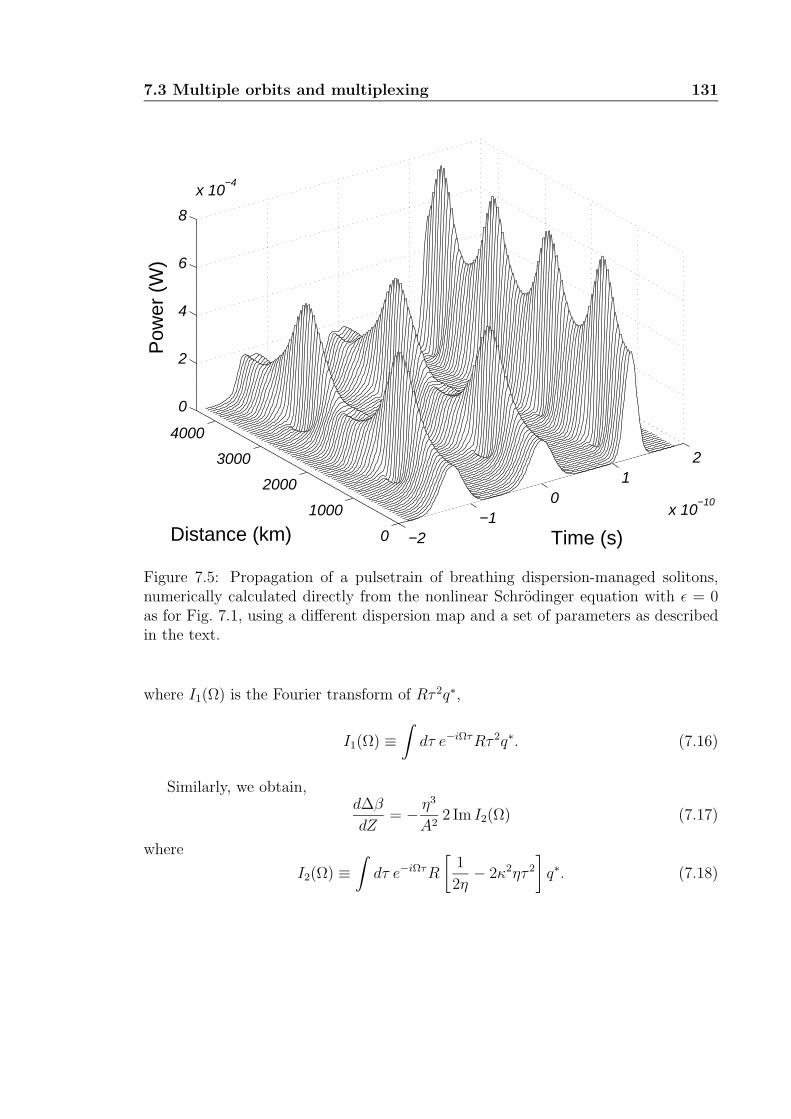
7.3 Multiple orbits and multiplexing 131
−2−1
01
2
x 10−10
0
1000
2000
3000
4000
0
2
4
6
8
x 10−4
Time (s)Distance (km)
Pow
er (
W)
Figure 7.5: Propagation of a pulsetrain of breathing dispersion-managed solitons,numerically calculated directly from the nonlinear Schrodinger equation with ε = 0as for Fig. 7.1, using a different dispersion map and a set of parameters as describedin the text.
where I1(Ω) is the Fourier transform of Rτ 2q∗,
I1(Ω) ≡∫
dτ e−iΩτRτ 2q∗. (7.16)
Similarly, we obtain,d∆β
dZ= − η3
A22 Im I2(Ω) (7.17)
where
I2(Ω) ≡∫
dτ e−iΩτR
[1
2η− 2κ2ητ 2
]q∗. (7.18)
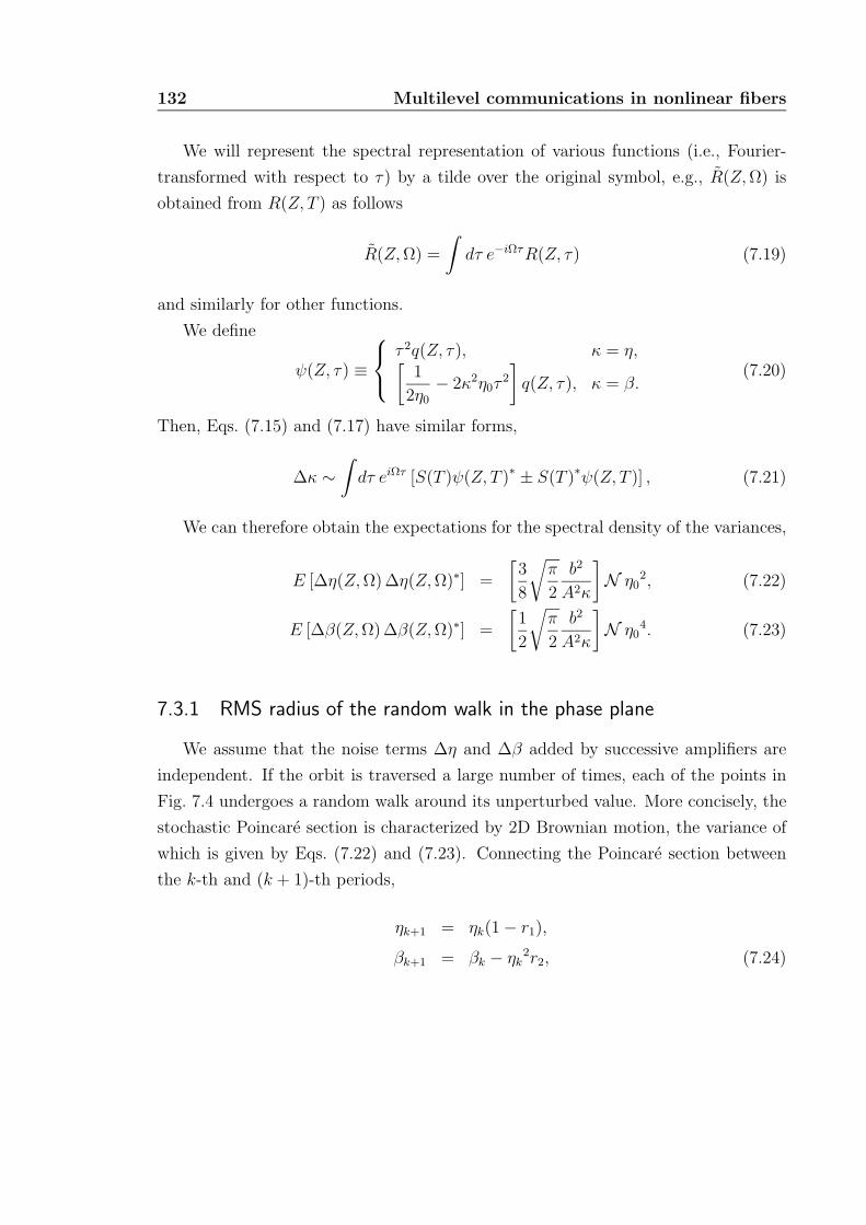
132 Multilevel communications in nonlinear fibers
We will represent the spectral representation of various functions (i.e., Fourier-
transformed with respect to τ) by a tilde over the original symbol, e.g., R(Z, Ω) is
obtained from R(Z, T ) as follows
R(Z, Ω) =
∫dτ e−iΩτR(Z, τ) (7.19)
and similarly for other functions.
We define
ψ(Z, τ) ≡
τ 2q(Z, τ), κ = η,[1
2η0
− 2κ2η0τ2
]q(Z, τ), κ = β.
(7.20)
Then, Eqs. (7.15) and (7.17) have similar forms,
∆κ ∼∫
dτ eiΩτ [S(T )ψ(Z, T )∗ ± S(T )∗ψ(Z, T )] , (7.21)
We can therefore obtain the expectations for the spectral density of the variances,
E [∆η(Z, Ω) ∆η(Z, Ω)∗] =
[3
8
√π
2
b2
A2κ
]N η0
2, (7.22)
E [∆β(Z, Ω) ∆β(Z, Ω)∗] =
[1
2
√π
2
b2
A2κ
]N η0
4. (7.23)
7.3.1 RMS radius of the random walk in the phase plane
We assume that the noise terms ∆η and ∆β added by successive amplifiers are
independent. If the orbit is traversed a large number of times, each of the points in
Fig. 7.4 undergoes a random walk around its unperturbed value. More concisely, the
stochastic Poincare section is characterized by 2D Brownian motion, the variance of
which is given by Eqs. (7.22) and (7.23). Connecting the Poincare section between
the k-th and (k + 1)-th periods,
ηk+1 = ηk(1 − r1),
βk+1 = βk − ηk2r2, (7.24)
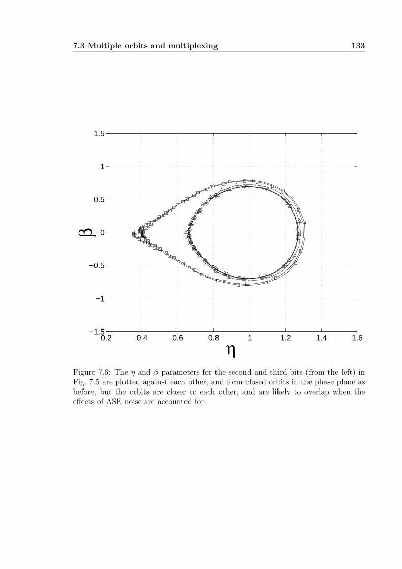
7.3 Multiple orbits and multiplexing 133
0.2 0.4 0.6 0.8 1 1.2 1.4 1.6−1.5
−1
−0.5
0
0.5
1
1.5
η
β
Figure 7.6: The η and β parameters for the second and third bits (from the left) inFig. 7.5 are plotted against each other, and form closed orbits in the phase plane asbefore, but the orbits are closer to each other, and are likely to overlap when theeffects of ASE noise are accounted for.
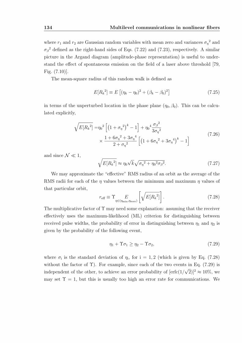
134 Multilevel communications in nonlinear fibers
where r1 and r2 are Gaussian random variables with mean zero and variances ση2 and
σβ2 defined as the right-hand sides of Eqs. (7.22) and (7.23), respectively. A similar
picture in the Argand diagram (amplitude-phase representation) is useful to under-
stand the effect of spontaneous emission on the field of a laser above threshold [79,
Fig. (7.10)].
The mean-square radius of this random walk is defined as
E[Rk2] ≡ E
[(ηk − η0)
2 + (βk − β0)2]
(7.25)
in terms of the unperturbed location in the phase plane (η0, β0). This can be calcu-
lated explicitly,
√E[Rk
2] =η02[(
1 + ση2)k − 1
]+ η0
4 σβ2
3ση2
× 1 + 6ση2 + 3ση
4
2 + ση2
[(1 + 6ση
2 + 3ση4)k − 1
] (7.26)
and since N 1, √E[Rk
2] ≈ η0
√k√
ση2 + η0
2σβ2. (7.27)
We may approximate the “effective” RMS radius of an orbit as the average of the
RMS radii for each of the η values between the minimum and maximum η values of
that particular orbit,
reff ≡ Υ Eη∈(ηmin,ηmax)
[√E[Rk
2]
]. (7.28)
The multiplicative factor of Υ may need some explanation: assuming that the receiver
effectively uses the maximum-likelihood (ML) criterion for distinguishing between
received pulse widths, the probability of error in distinguishing between η1 and η2 is
given by the probability of the following event,
η1 + Υσ1 ≥ η2 − Υσ2, (7.29)
where σi is the standard deviation of ηi, for i = 1, 2 (which is given by Eq. (7.28)
without the factor of Υ). For example, since each of the two events in Eq. (7.29) is
independent of the other, to achieve an error probability of [erfc(1/√
2)]2 ≈ 10%, we
may set Υ = 1, but this is usually too high an error rate for communications. We
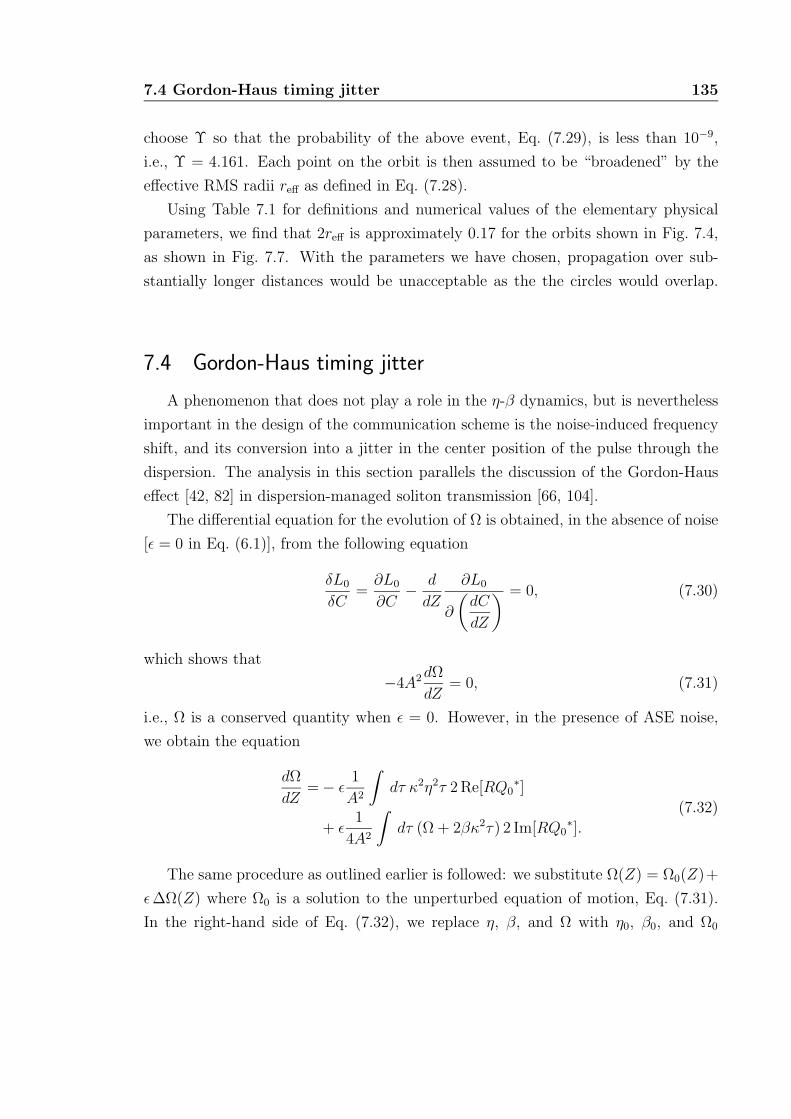
7.4 Gordon-Haus timing jitter 135
choose Υ so that the probability of the above event, Eq. (7.29), is less than 10−9,
i.e., Υ = 4.161. Each point on the orbit is then assumed to be “broadened” by the
effective RMS radii reff as defined in Eq. (7.28).
Using Table 7.1 for definitions and numerical values of the elementary physical
parameters, we find that 2reff is approximately 0.17 for the orbits shown in Fig. 7.4,
as shown in Fig. 7.7. With the parameters we have chosen, propagation over sub-
stantially longer distances would be unacceptable as the the circles would overlap.
7.4 Gordon-Haus timing jitter
A phenomenon that does not play a role in the η-β dynamics, but is nevertheless
important in the design of the communication scheme is the noise-induced frequency
shift, and its conversion into a jitter in the center position of the pulse through the
dispersion. The analysis in this section parallels the discussion of the Gordon-Haus
effect [42, 82] in dispersion-managed soliton transmission [66, 104].
The differential equation for the evolution of Ω is obtained, in the absence of noise
[ε = 0 in Eq. (6.1)], from the following equation
δL0
δC=
∂L0
∂C− d
dZ
∂L0
∂
(dC
dZ
) = 0, (7.30)
which shows that
−4A2dΩ
dZ= 0, (7.31)
i.e., Ω is a conserved quantity when ε = 0. However, in the presence of ASE noise,
we obtain the equation
dΩ
dZ= − ε
1
A2
∫dτ κ2η2τ 2 Re[RQ0
∗]
+ ε1
4A2
∫dτ (Ω + 2βκ2τ) 2 Im[RQ0
∗].(7.32)
The same procedure as outlined earlier is followed: we substitute Ω(Z) = Ω0(Z)+
ε ∆Ω(Z) where Ω0 is a solution to the unperturbed equation of motion, Eq. (7.31).
In the right-hand side of Eq. (7.32), we replace η, β, and Ω with η0, β0, and Ω0
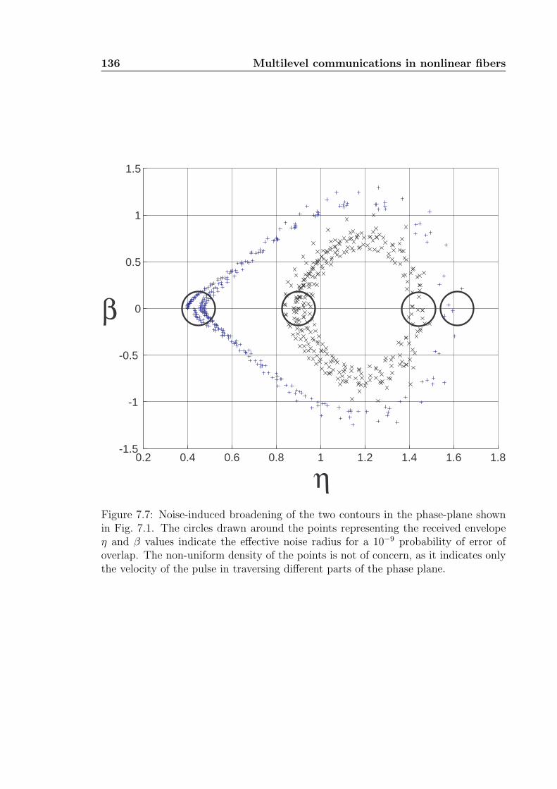
136 Multilevel communications in nonlinear fibers
0.2 0.4 0.6 0.8 1 1.2 1.4 1.6 1.8-1.5
-1
-0.5
0
0.5
1
1.5
η
β
Figure 7.7: Noise-induced broadening of the two contours in the phase-plane shownin Fig. 7.1. The circles drawn around the points representing the received envelopeη and β values indicate the effective noise radius for a 10−9 probability of error ofoverlap. The non-uniform density of the points is not of concern, as it indicates onlythe velocity of the pulse in traversing different parts of the phase plane.
7.4 Gordon-Haus timing jitter 137
which are the leading-order terms in the respective variables. Eq. (7.12) specifies the
perturbation R(Z, T ), and the spectral properties of S are given by Eq. (7.14).
In a similar fashion to the earlier analysis, we obtain the expectation for spectral
density of the variance of ∆Ω,
E [∆Ω ∆Ω∗] =κ2
A2
(η0
2 +1
4
β02
η02
+1
4
Ω02
κ2
)N . (7.33)
Similar to Eqs. (7.22) and (7.23), Eq. (7.33) characterizes the effect of a single
noise source. As evident from Fig. 7.7, the (η, β) locations of the amplifiers are
positioned randomly along the orbit. To obtain approximate analytical expressions,
we assume that the coordinates for the n-th amplifier (noise source) ηn and βn are
uniformly distributed and mutually independent random variables,
ηn ∼ U [ηmin, ηmax],
βn ∼ U [−βmax, βmax]n = 1, 2, . . . , N. (7.34)
where ηmin, ηmax, and βmax can be obtained from the results of simulations as shown
in Fig. 7.4.
The variance in the frequency Ω leads to a jitter in the temporal position of the
pulse: since the group delay is directly proportional to β′ ≡ dβ/dω [4], a change in the
group delay will be caused by a nonzero β′′∆ω [42, 82], or σ(z)∆Ω in our notation. If
we assume that the noise contributions of successive amplifiers are independent, the
overall jitter is given by [66]
E[∆T 2
]=∑
n
E [∆Ωn ∆Ωn∗][∫ NZa
nZa
dZ σ(Z)
]2
, (7.35)
where Za is the spacing between amplifiers, and N such amplifiers span the distance
between the source and the receiver (see Table 7.1).
Based on the discussion in the previous paragraph, we treat ηn2 etc. in the argu-
ment of the summation in the above equation as functions of uniformly distributed
random variables, and replace them with their expected values. We assume Ω0 = 0
corresponding to the ansatz used in Fig. 7.1. Since in this paper we only consider
fibers of uniform GVD, σ(Z) ≡ D, and assume equal spacing between amplifiers, the
138 Multilevel communications in nonlinear fibers
expression can be evaluated in closed-form,
E[∆T 2
]=D2N κ2
A2
ηmin
2 + ηminηmax + ηmax2
3
+βmax
2
12 ηmin ηmax
N(N + 1)(2N + 1)
6Za
2.
(7.36)
For large N , the last term in Eq. (7.36) is approximately (NZa)3/3Za, which iden-
tifies with the well-known cubic dependence of the Gordon-Haus jitter on the total
transmission length [42, Eq. (16)].
Kumar and Lederer [66] have commented that in dispersion-managed soliton sys-
tems that use several amplifiers within a period (i.e., noise sources are encountered
at different locations in the phase plane as in this analysis), a path-averaged inter-
pretation of the Gordon-Haus jitter is a good approximation to the actual dynamics.
This would be especially true here, since the period of the orbit is not the same as
the distance between two successive amplifiers.
To account for the normalizations implicit in Eq. (7.36), we multiply the expression
for E[∆T 2
]by the factor [1.665λ2/(2πc TFWHM)]2 [104]; the dimensions of this factor
are nm2 which account for the nm−2 from D2 in Eq. (7.36). Using numerical values
from Table 7.1, we evaluate the RMS timing jitter for the pulses described in Fig. 7.4:
κ = 1.18/1.76, A = 1.827, P0 = 1.57 mW,
LD =2πc
λ2D
(TFWHM
1.665
)2
= 318 km,
a(0) =
[2αZa
1 − exp(−2αZa)
]1/2
= 2.177
ηmin = 0.80, ηmax = 1.50 (7.37)
which leads to the RMS timing jitter,
∆TRMS ≡√
E[∆T 2
] ≈ 1.63 ps. (7.38)
For comparison, we have carried out 256 numerical simulations of pulse propaga-
tion similar to Fig. 7.7, and using a minimum squared residuals fitting algorithm, we
evaluate that E [∆T ] = 0.066 ps ≈ 0, i.e., zero mean, and ∆TRMS ≈ 2.38 ps. The
7.5 Comments 139
difference (0.75 ps) between the numerically evaluated RMS timing jitter and the
theoretical prediction is less than 0.5% of the inter-pulse time interval and less than
5% of the pulse width, which is very good agreement in light of the approximations
made in this analysis (Gaussian statistics, etc.)
A rule of thumb [82] is to allow a detection window of approximately six times the
RMS timing jitter for a bit-error-rate of 10−9. In the present case, this fits well within
the inter-pulse delay shown in Fig. 7.4, and additional filtering is not needed. The
Gordon-Haus jitter is not the dominant limitation with these parameters, but may
become more important if we use shorter pulses, or propagate over longer distances.
7.5 Comments
Our analysis so far has focused on the dynamics of pulse propagation in the
distributed amplifier approximation. In the case of lumped amplifiers, the pulse
amplitude experiences significant variations on a short length scale, and therefore, it
is convenient to factor out these variations using a(Z) as described in Section 7.1, and
in particular, by using Eq. (7.2). Since a(Z) also appears in Eq. (7.11), the phase-
plane dynamics are altered. Fig. 7.8 shows the change in the contour corresponding
to one of the orbits that was shown in Fig. 7.4. It is evident that the geometrical
structure of the phase plane is not altered and therefore the main conclusions of this
paper are equally valid, although the quantitative estimates must of course be re-
calculated. Further aspects of the differences will be discussed in a separate paper.
The goal of constellation design is simply to pick contours in the phase plane so
that their reff-widened orbits do not intersect, as shown by non-overlapping circles in
Fig. 7.7. In the language of nonlinear dynamic systems, we divide the space of orbits
S ∈ R2 into subsets Si each of which is invariant (stochastically, with 10−9 probability
of error) with respect to the flow of the initial value problem (IVP) vector field, i.e.,
for x = (η, β)T ,
If x(Z = 0) ≡ x0 ∈ Sk for a particular k
then Prx(Z) /∈ Sk ≤ 10−9 for all Z. (7.39)
In the example that we have used for illustrative purposes in this paper, there are
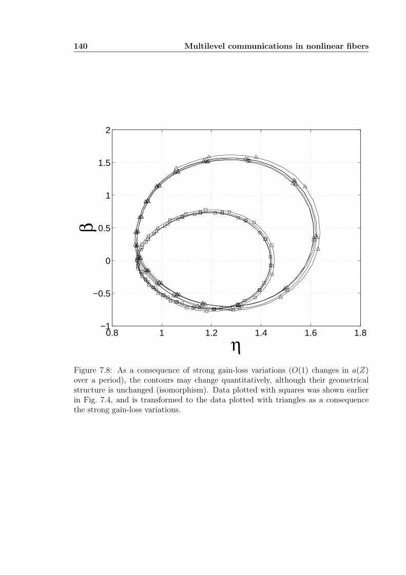
140 Multilevel communications in nonlinear fibers
0.8 1 1.2 1.4 1.6 1.8−1
−0.5
0
0.5
1
1.5
2
η
β
Figure 7.8: As a consequence of strong gain-loss variations (O(1) changes in a(Z)over a period), the contours may change quantitatively, although their geometricalstructure is unchanged (isomorphism). Data plotted with squares was shown earlierin Fig. 7.4, and is transformed to the data plotted with triangles as a consequencethe strong gain-loss variations.
7.5 Comments 141
four multiplexing levels defined by the four circles in Fig. 7.7. These additional levels
of multiplexing arise from the nonlinear evolution of the pulse in the phase-plane;
critical to their existence is the fact that the Kerr nonlinearity acts in a deterministic
manner, and is not merely one of the noise terms as in conventional wavelength-
division multiplexing (WDM) transmission formats.
Such a multiplexing scheme is best utilized if receivers can reliably detect the
quadratic chirp of the received pulse in real time and with milliwatt pulse powers [137].
Then more than four multiplexing levels can be allowed by selecting non-overlapping
neighborhoods for the parameters at the output of the channel. These neighborhoods
are isomorphic to circles in R2 or n-balls in R
n. The ultimate limits of such multi-
plexing are directly related to sphere (or ellipsoid) packing problems in n-dimensions,
where n is the number of statistically significant parameters. For shorter distances,
more levels may be defined since the noise radii are smaller.
7.5.1 Optimum amplifier gain for fixed total distance
For a fixed distance L between source and receiver, the number of amplifier stages
is L/Za which can be re-written in terms of the amplifier gain G as αL/ log G, where
α is the attenuation per unit length of the fiber. Clearly, the number of noise sources
encountered by the pulse is inversely proportional to the gain of the amplifiers, G.
On the other hand, the noise radius increases with G, since higher gain amplifiers
add more ASE noise to the signal [154].
From Eq. (7.27), we can write, as a function of G,
reff(G) ∼[G − 1
log G
]1/2
reff, G ≥ 1. (7.40)
where reff is independent of G. Note that the noise radius increases, and therefore
fewer levels of multiplexing are allowed, if high gain amplifiers are used. Further,
limG→1
reff(G) = reff, (7.41)
which is the minimum noise radius that can be achieved, i.e., in the limit of a lossless
channel. It is interesting that the figure-of-merit for a prototypical linear optical
transmission shows a similar behavior [153].
142 Multilevel communications in nonlinear fibers
In contrast with the proposal by Hasegawa and Nyu [45] for a different nonlinear
multiplexing scheme using (non dispersion-managed) solitons, this scheme does not
require that the information-carrying parameters (η and β) are unchanged during
the course of transmission, but merely that a receiver can clearly distinguish, at its
specific location, between their values corresponding to different codes. In addition,
this scheme explicitly accounts for dispersion-managed fiber links; this is significant
in light of the considerable spans of normal-dispersion fiber already installed in com-
mercial networks.
Higher-dimensional generalizations are richer analytically, but with greater com-
plications in the dynamical evolution. The behavior in the vicinity of non-hyperbolic
critical points (such as the center in the phase plane for the AD fibers) requires a
more sophisticated analysis of the behavior on the central manifold, using normal
form theory, and may result in chaotic behaviour in certain circumstances. If the
section of the phase plane in which we define the channel contains several compound
separatrix cycles (graphics), with the separatrixes homoclinic to the origin (e.g., the
topology of the n-bouquet), this would allow zones of multiplexing, with a reduced
probability of crossing zones. The physical (design) implications of such topologies
are a current research topic.
Each particular implementation has particular features that deserve special atten-
tion. In optical transmission, for example, interactions between nonlinearly-multiplexed
pulses have been suppressed, since we have taken the nonlinear multiplexing to be
super-imposed on top of a WDM and TDM specification. This scheme precludes
strong interactions between two pulses with the same carrier frequency and in the
same time slot. But multiaccess channels do not typically maximize capacity by or-
thogonal multiplexing techniques. Optimizing the design of systems in the presence of
multiaccess interference in nonlinear channels is an open problem. Optical filtering
will probably be implemented in the transmission channel to suppress out-of-band
radiation and the accumulation of dispersive waves, and to guide the evolution of the
nonlinear pulseshapes along desired trajectories.
7.5 Comments 143
We have introduced a new format for multiplexed signal transmis-
sion dispersion-managed optical fiber communication systems which
constructively utilizes the group-velocity dispersion and Kerr nonlin-
earity present in commonly-used optical fibers. This scheme, called
PulseWidth and Chirp Division Multiplexing (PWCDM), is based on the
evolution of the chirp and amplitude (width) parameters describing the
pulse envelope in the phase plane, most conveniently characterized us-
ing a variational approach. Amplified spontaneous emission (ASE) noise
from optical amplifiers results in amplitude and chirp jitter, and deter-
mines the selection of appropriate multiplexing levels and the design of
the signalling constellation. In addition, ASE also results in the Gordon-
Haus timing jitter, and if this effect is not compensated, an additional
constraint may be imposed on the interpulse temporal separation.

144 Multilevel communications in nonlinear fibers
Chapter 8
Space-time analogies in pulse propagation
With the successes of the Glashow-Weinberg-Salam theory of electroweakinteractions, the renormalizability proof of gauge theories by t’Hooft,
and the developments of QCD, it is now universally accepted that all interactionsare based on the gauge principle. I had coined the phrase
Symmetry Dictates Interactions to describe this view about the role thatsymmetry plays in the conceptual structure of nature’s fundamental forces,
a view that is a dominant theme of contemporary physics.
—C. N. Yang, Gauge Fields I, Proc. 20th Int. SchoolSubnuclear Phys. (Ettore Majorana), Erice (1982).
This chapter is an ab initio study of pulse propagation phenomena analogous to
spatial CW diffraction behavior. We address both linear dispersive evolution as well
the self-phase modulation effects of the nonlinear index of refraction [29]. The latter
is responsible for much of the current interest in nonlinear optical communications,
since pulse shapes such as solitons and dispersion-managed solitons display much more
attractive transmission properties than linear transmission formats (e.g., NRZ) [22].
Such nonlinear pulses are usually self-consistent eigensolutions of a wave equa-
tion, which is the primary reason for their robustness to uncompensated spectral
broadening and resultant dissipation into the continuum. The conventional hyper-
bolic secant soliton is an exact solution of the nonlinear Schrodinger equation [4], and
propagates indefinitely in a lossless medium without losing its shape. Lossless media
can be realized in practice quite effectively by using lumped amplification stages, and
erbium-doped fiber amplifiers offer excellent characteristics in this regard.
Breathers, sometimes called dispersion-managed solitons [135, 128], are also self-
consistent eigensolutions of the wave equation that propagate with periodic pulse
width, chirp, etc., but do not require that the governing system of equations is in-
tegrable. While not strictly unchanging in shape, breathers are self-trapped—evolve
145
146 Space-time analogies in pulse propagation
back to their initial configuration, essentially traversing a closed, nondegenerate orbit
in phase space [68]. Unlike pulse shapes designed for linear transmission channels,
these pulses do not require periodic dispersion compensation along the transmission
channel, and so offer an attractive alternative to the strong control requirements of
the nonlinear Schrodinger soliton.
Characterizing the solutions of the nonlinear wave equation is often simplest via
direct numerical simulation, and this has been particularly true for dispersion mapped
solitons [81]. In order to understand, capture, and then predict and utilize the es-
sential physics that guides this behavior, a more conceptually accessible framework is
sometimes preferable, such as the variational approach with a pulse shape Ansatz [7].
The pulse shape is described as a dynamical system; we write the Hamiltonian based
on the action principle and seek solutions to the Euler-Lagrange equations of mo-
tion [100, 39]. This approach is not always applicable, however, especially when the
Ansatz is incapable of capturing some essential physical behavior. Also, it is some-
what more of an analytical tool for probing the dynamics of systems that we already
know something about, or can predict at least partially, and it may be convenient to
have other approaches that can offer quick insight into constructive aspects of nonlin-
ear propagation, so that different geometries can be analyzed and compared quickly
and easily.
The parallels between dispersive pulse propagation in optical fibers and paraxial
CW Gaussian beam diffraction in free space have been identified for some time [5, 157,
14]. More recently, the analogies have been extended to include temporal lenses as a
way to translate the imaging properties of spatial lenses into the temporal domain [65].
In this way, pulse correlation and convolution devices may also be constructed [77].
Still more recently, it was shown that temporal lenses can characterize nonlinear
effects in the wave equation, leading for example, to the formation of a class of
steady-state repeating pulses [155]. This is perhaps the most potentially useful of
the space-time analogies, and in this chapter, we will discuss a further extension of
this formalism to describe still more powerful applications such as Gaussian pulse
propagation in dispersion-managed optical fiber systems, including the effects of the
nonlinear index of refraction.
8.1 Gaussian beam diffraction and pulse propagation 147
8.1 Gaussian beam diffraction and pulse propagation
Consider the diffraction of an electromagnetic field E(x, z, t) of carrier frequency
ω and scalar complex amplitude u(x, z), which obeys the Helmholtz equation
∇2u + k2u = 0, k2 = ω2µε =
(2πn
λ
)2
. (8.1)
In the paraxial approximation, we consider only those optical beams whose plane
wave components propagate at small angles to the z axis [154],
u(z, t) =
√ik
2πz
∫u0(x
′) exp
[− ik
2z(x − x′)2
]dx′, (8.2)
where u0(x) is the envelope of the field at z = 0.
The propagation of CW Gaussian beams in free space and rotationally symmetric
quadratic graded-index media is conveniently described by assuming that the envelope
has the form [154]
u = exp
−i
[P (z) +
k
2q(z)r2
](8.3)
where we find by substitution into the wave equation (8.1) that dP/dz = −i/q(z) for
such media. The q-parameter describes the Gaussian beam completely,
1
q(z)=
1
R(z)− i
λ
πnw2(z). (8.4)
In the above definition, R(z) describes the radius of curvature of the beam and w(z)
describes the beam spot size.
The usefulness of the q parameter lies in the bilinear transformation (ABCD law)
that characterizes how this parameter evolves with propagation. For an optical system
described by a real (or complex) 2 × 2 ABCD matrix, the output q parameter qo is
given by
qo =Aqi + B
Cqi + D, (8.5)
in terms of the input q parameter qi. The real and imaginary parts of qo describe
the radius of curvature and spot size of the Gaussian beam at the output of the
optical system. Many practically important optical systems and their corresponding
148 Space-time analogies in pulse propagation
Spatial frequency (Fourier variable) kx Ω frequency (Fourier variable)Transverse distance x t − z
vgtime (moving ref. frame)
Propagation distance z z propagation distanceWave vector (inverse) k−1 −β′′ GVD coefficient (negative)
Table 8.1: Space-time translation rules.
phenomena can be described by simple ABCD matrices, such as propagation in a
uniform medium, focusing via a thin lens, beam transformation at a dielectric inter-
face, propagation through a curved dielectric interface and thick lens, propagation in
a medium with a quadratic index variation, etc. [154, Table 2-1].
In the temporal case, a single mode in an optical fiber (usually the lowest-order
fundamental mode) can be written in terms of the wavenumber β0,
E(z, t) = u(z, t) exp[i(ω0t − β0z)], (8.6)
assuming that the optical field is quasi-monochromatic centered at ω0. The differential
equation satisifed by u is, to second order of derivatives with respect to the optical
frequency ω of the mode propagation constant β(ω) [4],
∂u
∂z+ β′∂u
∂t+
1
2β′′∂
2u
∂t2= 0. (8.7)
The solution to the above equation is [156]
u(z, t) =
√1
i2πβ′′z
∫u0(t
′) exp
[i
2β′′z(T − t′)2
]dt′, (8.8)
where T = t−β′z = t−z/vg is the time coordinate in the frame of reference comoving
with the pulse envelope at the group velocity vg = 1/β′, and u0(t) is the envelope at
z = 0. Group-velocity dispersion (GVD) is represented by the parameter β′′.
The formal similarity between Eqs. (8.2) and (8.8) is the principal motivation for
this analysis. We can write down a set of space-time translation rules (see Table 8.1)
to apply results from spatial diffraction to temporal dispersion and vice versa. One
family of results that can be derived from this space-time analogy corresponds to
spatial imaging, e.g., the 2-f and 4-f optical systems. These can be applied to pulse
compression or expansion experiments, etc. [65].
8.2 The ABCD formalism for Gaussian pulses 149
But we will see in later sections that many linear and nonlinear pulse propagation
systems can be described by cascading simple ABCD matrices, and this can result
in substantially simpler calculations and more direct physical understanding of the
physical processes involved in nonlinear pulse propagation. We will first need to
develop some additional facility in characterizing optical systems associated with the
pulse propagation equations.
The spatial q-parameter has a temporal equivalent qt in accordance with the space-
time translation rules of Table 8.1 defined by
1
qt(z)=
1
Rt(z)+ i
2β′′
τ 2(z), (8.9)
where τ(z) represents the pulse width (scaled in the T frame by√
2) and Rt(z) is
its chirp. A Gaussian pulse in linearly dispersive fibers is then represented by the
envelope [156]
u(z, t) = u0τ0
τ(z)exp
[i tan−1 z
ζ0
+ it2
2β′′Rt(z)+
β′′
|β′′|t2
τ 2(z)
], (8.10)
where the pulse width and chirp satisfy evolution equations in linear dispersive fibers
exactly analogous to their spatial counterparts, beam spot size and radius of curva-
ture, in free space [155]
τ 2(z) = τ 20
(1 +
z2
ζ20
),
Rt(z) = z
(1 +
ζ20
z2
), (8.11)
with ζ0 = τ 20 /2|β′′| defining the dispersion length [4].
8.2 The ABCD formalism for Gaussian pulses
As a simple example of the application of the above translation rules, we consider
the propagation of a Gaussian input pulse with envelope
U(0, T ) = exp
(− T 2
2 T02
). (8.12)
150 Space-time analogies in pulse propagation
The transmission medium comprises two concatenated sections of fiber with lengths
z1 and z2 and with GVD coefficients β′′1 and β′′
2 respectively. We ignore any nonlinear
effects in this simple problem and assume that the medium is lossless. We will de-
termine the pulse characteristics at the output of the second medium, i.e., the pulse
width at z = z1 + z2.
One way of solving this problem is by recourse to the wave equation solution
Eq. (8.8) by the Fourier transform technique. We have
U(z2, Ω) = U(z1, Ω) exp
(i
2β′′
2z1Ω2
)
= U(z0, Ω) exp
[i
2(β′′
1z1 + β′′2z2) Ω2
]. (8.13)
Taking the inverse Fourier transform,
U(z1 + z2, T ) =1
2π
∫ ∞
−∞U(0, Ω) exp
[i
2(β′′
1z1 + β′′2z2) Ω2 − iΩT
]dΩ
=
[T0
2
T02 − i(β′′
1z1 + β′′2z2)
]1/2
exp
[− T 2
2(T02 − i(β′′
1z1 + β′′2z2)
],
(8.14)
from which we see that the ratio of the output to input pulse width is
T1
T0
=
[1 +
(β′′
1z1 + β′′2z2
T02
)2]1/2
. (8.15)
We will now verify Eq. (8.15) using the ABCD matrix approach. The system is
described very simply by the product of three matrices,
M =
(1 z2
0 1
)(1 0
0β′′2
β′′1
)(1 z1
0 1
)
=
(1 z1 +
β′′2
β′′1z2
0β′′2
β′′1
)(8.16)
so that
q2 =Aq1 + B
Cq1 + D=
β′′1
β′′2
q1 +β′′
1
β′′2
z1 + z2. (8.17)
8.2 The ABCD formalism for Gaussian pulses 151
Using the shorthand notation
R2 ≡ R(z1 + z2), R1 ≡ R(0),
τ2 ≡ τ(z1 + z2), τ1 ≡ τ(0),(8.18)
we have1
R2− i
2β′′2
τ22(
1R2
)2
+(
2β′′2
τ22
)2 =β′′
1
β′′2
1R1
− i2β′′
1
τ21(
1R1
)2
+(
2β′′1
τ21
)2 +β′′
1
β′′2
z1 + z2. (8.19)
The real and imaginary parts of both sides of the above equation have to be equal,
leading to a pair of simultaneous equations. For an unchirped input pulse, R1 = 0 so
that equality of the imaginary parts leads to
(1
R2
)2
+
(2β′′
2
τ 22
)2
=
(2β′′
2
τ2τ1
)2
.
Substituting this expression into the equation of equality of the real parts of Eq. (8.19)
and some algebraic manipulation leads to
τ(z1 + z2)
τ(0)=
τ2
τ1
=
[1 +
(β′′
1z1 + β′′2z2
τ 21 /2
)2]1/2
, (8.20)
which is the same as Eq. (8.15), since τ =√
2 ∆T .
In the above calculation, we have carried out some algebraic simplifications by
hand in order to show that the result obtained by the ABCD matrix approach is the
same as that obtained by the Fourier transform approach. Nevertheless, the former
is computationally much simpler, and separating the real and imaginary parts of
Eq. (8.19) as part of a numerical algorithm can be carried out without the notational
complexity of, for example, rationalizing the denominator.
Our ABCD formalism would be of limited interest if the only phenomena it could
capture were that of dispersive propgation.The time-lens formalism lets us describe
nonlinear mechanisms as well. By analogy to spatial lenses that are characterized by
a lens factor exp(ikr2/2f) which multiplies an incoming optical beam, we define a
temporal lens as a device that multiplies the pulse envelope by a factor [155, 65]
Lens Factor = exp
[−i
t2
2β′′ft
]≡ exp
[−ibt2]. (8.21)
152 Space-time analogies in pulse propagation
The ABCD matrix representing a temporal lens has the same form as that of a
spatial lens,
M =
(1 0
− 1ft
0
), (8.22)
where ft represents the temporal “focal length.”
A comparison of spatial and temporal lensing is shown in Fig. 8.1. In the spatial
case, the lens compensates for the spreading of the beam waist and “flips” the phase
fronts to convert a diverging beam into a converging one. Similarly, a temporal lens
reverses the sign of the chirp, so that further propagation in a β′′ < 0 dispersive
fiber will compensate for the chirp (phase modulation) caused this far. This is also
an interesting and physically illuminating approach to discussing the physics of the
formation of solitons [154, Chap. 19].
One possible implementation, as proposed in [155], is to achieve temporal lensing
by self-phase modulation during the passage of the pulse through a section of nonlinear
fiber (β′′ ≈ 0, n2 > 0). For short distances, z πτ02/|β′′| and when β′′/τ0
2 (2πn2/λ)Ip for peak intensity Ip, a pulse with input electric field envelope u(0, T )
emerges from a length z of nonlinear fiber with phase modulation
u(z, T ) = u(0, T ) exp
[−i
ω0n2z
2cη|u(0, T )|2
](8.23)
where η =√
µ/ε defines the impedance of free space. We write the pulse intensity as
I =|u|22η
= Ip exp
[−2
(T
τ0
)2]
, (8.24)
and keep the first two terms in the Taylor expansion of the exponential in Eq. (8.23),
u(z, T ) = u(0, T ) exp
[i2ω0n2Ipz
cτ02
T 2
], (8.25)
modulo a phase term linear in z that is independent of T . The effect of propagation
through length L of nonlinear fiber is to impart a quadratic chirp to the pulse, which
we represent by the multiplicative term exp(−ibt2) so that
b =1
2β′′ft
= −2ω0n2IpL
cτ02
. (8.26)
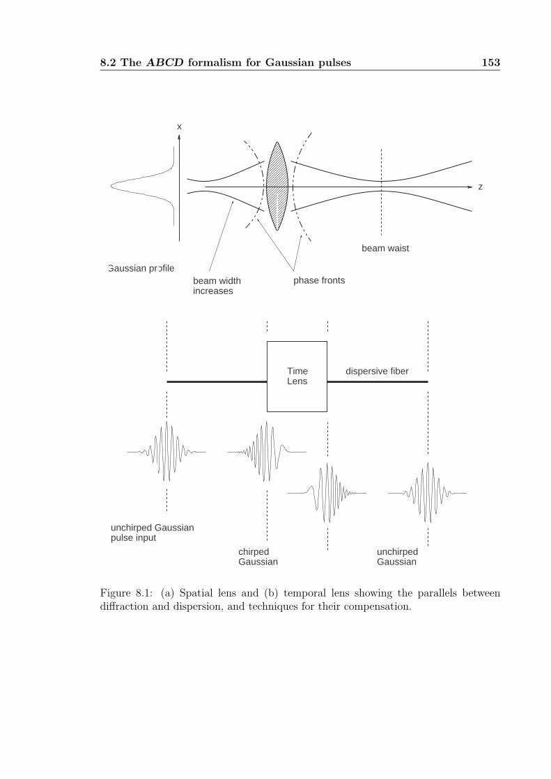
8.2 The ABCD formalism for Gaussian pulses 153
xxxxxxxxxxxxxxxxxxxxxxxxxxxxxxxxxxxxxxxxxxxxxxxxxxxxxxxxxxxxxxxxxxxxxxxxxxxxxxxxxxxxxxxxxxxxxxxxxxxxxxxxxxxxxxxxxxxxxxxxxxxxxxxxxxxxxxxxxxxxxxxxxxxxxxxxxxxxxxxxxxxxxxxxxxxxxxxxxxxxxxxxxxxxxxxxxxx
xxxxxxxxxxxxxxxxxxxxxxxxxxxxxxxxxxxxxxxxxxxxxxxxxxxxxxxxxxxxxxxxxxxxxxxxxxxxxxxxxxxxxxxxxxxxxxxxxxxxxxxxxxxxxxxxxxxxxxxxxxxxxxxxxxxxxxxxxxxxxxxxxxxxxxxxxxxxxxxxxxxxxxxxxxxxxxxxxxxxxxxxxxxxxx
phase fronts
beam waist
Gaussian profile
x
z
beam widthincreases
TimeLens
unchirped Gaussianpulse input
dispersive fiber
chirpedGaussian
unchirpedGaussian
Figure 8.1: (a) Spatial lens and (b) temporal lens showing the parallels betweendiffraction and dispersion, and techniques for their compensation.
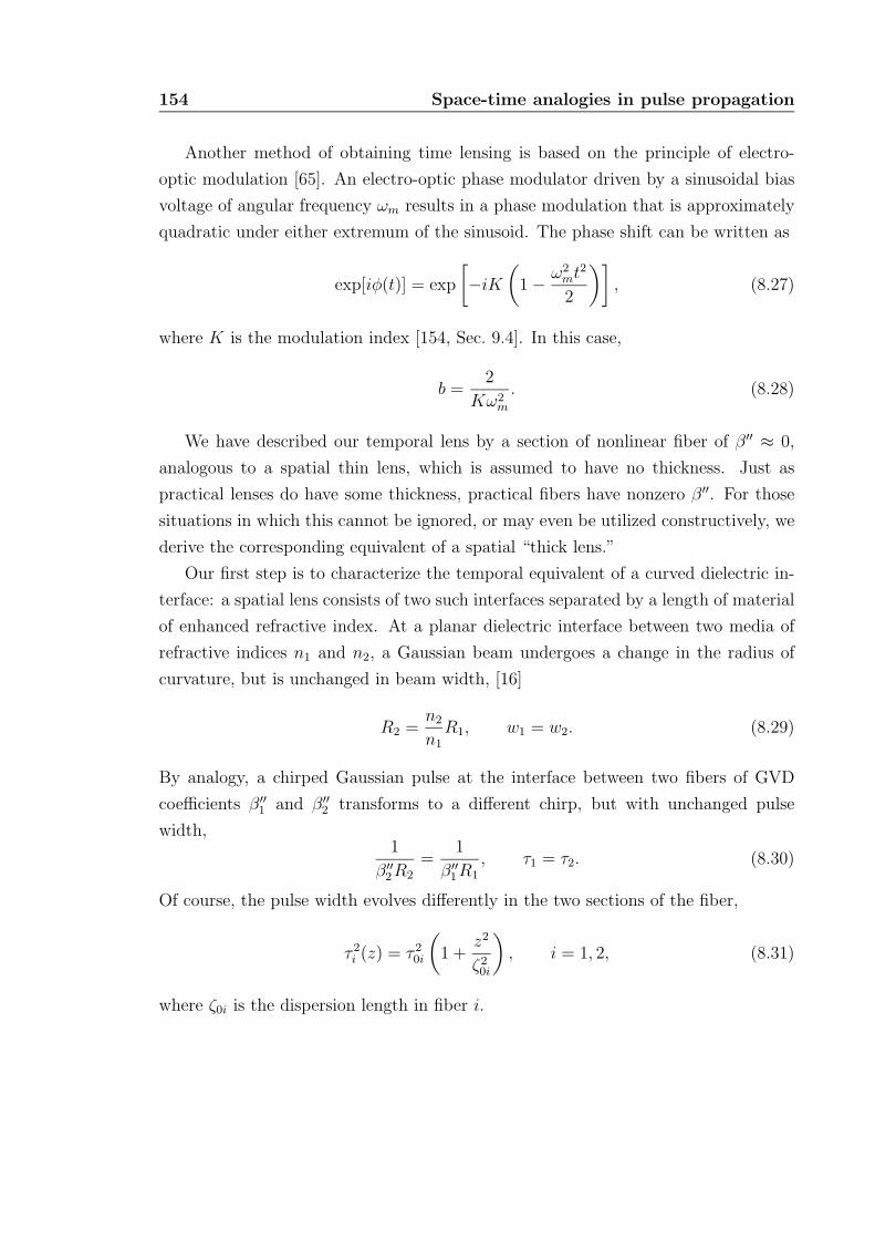
154 Space-time analogies in pulse propagation
Another method of obtaining time lensing is based on the principle of electro-
optic modulation [65]. An electro-optic phase modulator driven by a sinusoidal bias
voltage of angular frequency ωm results in a phase modulation that is approximately
quadratic under either extremum of the sinusoid. The phase shift can be written as
exp[iφ(t)] = exp
[−iK
(1 − ω2
mt2
2
)], (8.27)
where K is the modulation index [154, Sec. 9.4]. In this case,
b =2
Kω2m
. (8.28)
We have described our temporal lens by a section of nonlinear fiber of β′′ ≈ 0,
analogous to a spatial thin lens, which is assumed to have no thickness. Just as
practical lenses do have some thickness, practical fibers have nonzero β′′. For those
situations in which this cannot be ignored, or may even be utilized constructively, we
derive the corresponding equivalent of a spatial “thick lens.”
Our first step is to characterize the temporal equivalent of a curved dielectric in-
terface: a spatial lens consists of two such interfaces separated by a length of material
of enhanced refractive index. At a planar dielectric interface between two media of
refractive indices n1 and n2, a Gaussian beam undergoes a change in the radius of
curvature, but is unchanged in beam width, [16]
R2 =n2
n1
R1, w1 = w2. (8.29)
By analogy, a chirped Gaussian pulse at the interface between two fibers of GVD
coefficients β′′1 and β′′
2 transforms to a different chirp, but with unchanged pulse
width,1
β′′2R2
=1
β′′1R1
, τ1 = τ2. (8.30)
Of course, the pulse width evolves differently in the two sections of the fiber,
τ 2i (z) = τ 2
0i
(1 +
z2
ζ20i
), i = 1, 2, (8.31)
where ζ0i is the dispersion length in fiber i.
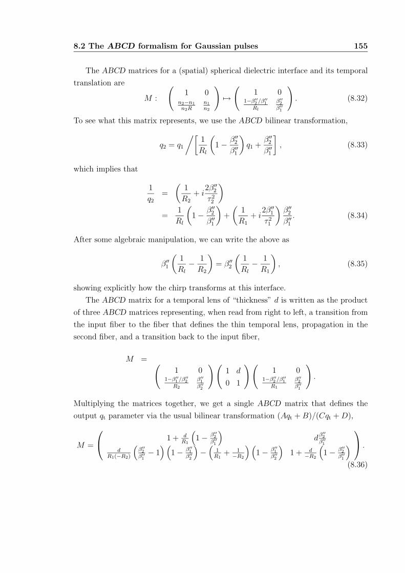
8.2 The ABCD formalism for Gaussian pulses 155
The ABCD matrices for a (spatial) spherical dielectric interface and its temporal
translation are
M :
(1 0
n2−n1
n2Rn1
n2
)→(
1 01−β′′
2 /β′′1
Rl
β′′2
β′′1
). (8.32)
To see what this matrix represents, we use the ABCD bilinear transformation,
q2 = q1
/[1
Rl
(1 − β′′
2
β′′1
)q1 +
β′′2
β′′1
], (8.33)
which implies that
1
q2
=
(1
R2
+ i2β′′
2
τ 22
)
=1
Rl
(1 − β′′
2
β′′1
)+
(1
R1
+ i2β′′
1
τ 21
)β′′
2
β′′1
. (8.34)
After some algebraic manipulation, we can write the above as
β′′1
(1
Rl
− 1
R2
)= β′′
2
(1
Rl
− 1
R1
), (8.35)
showing explicitly how the chirp transforms at this interface.
The ABCD matrix for a temporal lens of “thickness” d is written as the product
of three ABCD matrices representing, when read from right to left, a transition from
the input fiber to the fiber that defines the thin temporal lens, propagation in the
second fiber, and a transition back to the input fiber,
M = (1 0
1−β′′1 /β′′
2
R2
β′′1
β′′2
)(1 d
0 1
)(1 0
1−β′′2 /β′′
1
R1
β′′2
β′′1
).
Multiplying the matrices together, we get a single ABCD matrix that defines the
output qt parameter via the usual bilinear transformation (Aqt + B)/(Cqt + D),
M =
1 + d
R1
(1 − β′′
2
β′′1
)d
β′′2
β′′1
dR1(−R2)
(β′′2
β′′1− 1
)(1 − β′′
1
β′′2
)−(
1R1
+ 1−R2
)(1 − β′′
1
β′′2
)1 + d
−R2
(1 − β′′
2
β′′1
) .
(8.36)
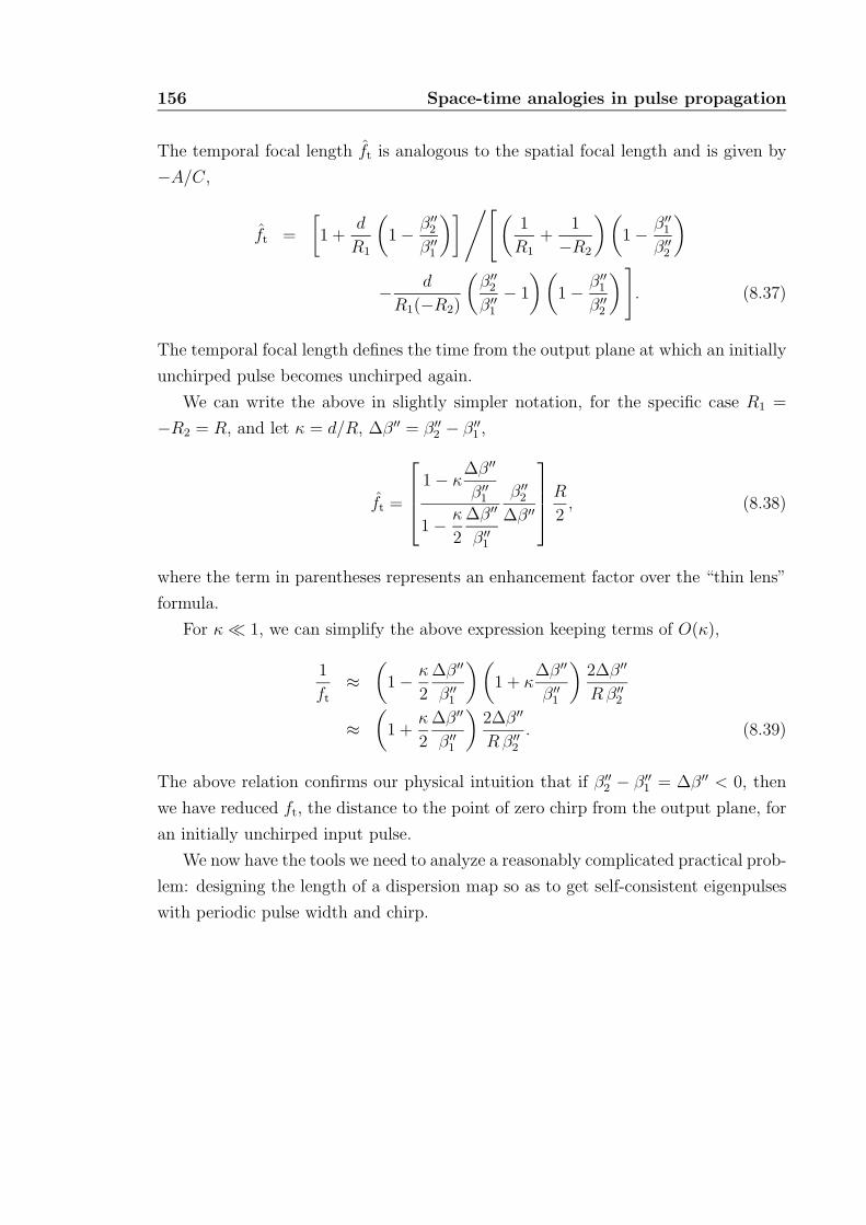
156 Space-time analogies in pulse propagation
The temporal focal length ft is analogous to the spatial focal length and is given by
−A/C,
ft =
[1 +
d
R1
(1 − β′′
2
β′′1
)]/[(1
R1
+1
−R2
)(1 − β′′
1
β′′2
)
− d
R1(−R2)
(β′′
2
β′′1
− 1
)(1 − β′′
1
β′′2
)]. (8.37)
The temporal focal length defines the time from the output plane at which an initially
unchirped pulse becomes unchirped again.
We can write the above in slightly simpler notation, for the specific case R1 =
−R2 = R, and let κ = d/R, ∆β′′ = β′′2 − β′′
1 ,
ft =
1 − κ∆β′′
β′′1
1 − κ
2
∆β′′
β′′1
β′′2
∆β′′
R
2, (8.38)
where the term in parentheses represents an enhancement factor over the “thin lens”
formula.
For κ 1, we can simplify the above expression keeping terms of O(κ),
1
ft
≈(
1 − κ
2
∆β′′
β′′1
)(1 + κ
∆β′′
β′′1
)2∆β′′
R β′′2
≈(
1 +κ
2
∆β′′
β′′1
)2∆β′′
R β′′2
. (8.39)
The above relation confirms our physical intuition that if β′′2 − β′′
1 = ∆β′′ < 0, then
we have reduced ft, the distance to the point of zero chirp from the output plane, for
an initially unchirped input pulse.
We now have the tools we need to analyze a reasonably complicated practical prob-
lem: designing the length of a dispersion map so as to get self-consistent eigenpulses
with periodic pulse width and chirp.
8.3 DM soliton transmission experiment 157
8.3 DM soliton transmission experiment
It has been recently found that a stable, self-consistent pulse solution exists in
a dispersion-managed fiber transmission system [128]. While these are not solitons
in the strict mathematical sense, they have been called dispersion-managed solitons
or perhaps more appropriately, breathers. They demonstrate periodic behavior: the
pulse width and chirp of Gaussian breathers, for instance, are periodic functions of the
propagation distance. Breathers share a property in common with solitons, in that
they can propagate indefinitely without losing shape; even though the pulse shape
undergoes changes within a dispersion map period, the pulse does not disperse away
to infinity or tend to self-focus to a point, either of which invalidate the applicability
of the nonlinear Schrodinger equation after a certain distance.
A dispersion-managed (DM) soliton is closer to a Gaussian shape than the hy-
perbolic secant of the nonlinear Schrodinger equation [73], and it is interesting to
ask whether our analysis is capable of capturing the essential aspects of its evolution
along a dispersion-managed transmission channel.
We consider, as our example, the paper by Mu et al. [97] who have simulated
DM soliton dynamics in a recirculating fiber loop. Their dispersion map consists
of 100 km of dispersion shifted fiber (SMF-LS) with normal dispersion D1 equal to
-1.10 ps/nm-km at 1551 nm, followed by an “approximately 7 km span” of standard
single-mode fiber (SMF-28) with an anomalous dispersion D2 equal to 16.6 ps/nm-km
at 1551 nm. The results of the paper indicate that Gaussian shaped pulses of pulse
duration 5.67 ps and peak power 9 dBm were used. We will derive the result that,
for these parameters and given the length of SMF-LS fiber, the length of SMF-28
fiber that needs to be used is indeed “approximately 7 km.” In other words, we
will show that this given dispersion map can support lowest-order chirped Gaussian
self-consistent solutions, i.e., breathers.
The dispersion map, shown schematically in Fig. 8.2, consists of three fiber seg-
ments: a length z1/2 equal to 50 km of SMF-LS fiber, followed by a length z2 of
SMF-28 fiber whose numerical value is to be determined, and then the remainder
z1/2 of SMF-LS fiber. Each segment of fiber has nonlinear characteristics, which we
model via a time lens situated for simplicity at the individual midpoints of the re-
spective segments. Consequently, each segment is described by the cascaded product
of three ABCD matrices, with two additional matrices representing the transitions
158 Space-time analogies in pulse propagation
between fibers of different β′′. For simplicity, we will assume that the nonlinear
properties of the fibers are identical.
The overall ABCD matrix for the system can be written as the product of the
following eleven matrices,
M =
(1 z1/4
0 1
)(1 0
−1/ft 1
)(1 z1/4
0 1
)(1 0
0 β′′1/β′′
2
)(
1 z2/2
0 1
)(1 0
−1/ft 1
)(1 z2/2
0 1
)(1 0
0 β′′2/β′′
1
)(
1 z1/4
0 1
)(1 0
−1/ft 1
)(1 z1/4
0 1
), (8.40)
which after some algebra can be written as a single 2 × 2 ABCD matrix with the
following elements,
A =
[(1 − z1
4f
)(1 − z2
2f
)− z1
4f
β′′1
β′′2
(2 − z1
4f
)](1 − z1
4f
)(8.41)
−[β′′
2
β′′1
(1 − z1
4f
)(2 − z2
2f
)z2
2f+
(2 − z1
4f
)(1 − z2
2f
)z1
4f
],
B =
[(1 − z1
4f
)(1 − z2
2f
)− z1
4f
β′′1
β′′2
(2 − z1
4f
)]z1
4
(2 − z1
4f
)(8.42)
+
[β′′
2
β′′1
(1 − z1
4f
)(2 − z2
2f
)z2
2+
(2 − z1
4f
)(1 − z2
2f
)z1
4
](1 − z1
4f
),
C = − 1
f
[(1 − z2
2f
)+
β′′1
β′′2
(1 − z1
4f
)](1 − z1
4f
)(8.43)
− 1
f
[−β′′
2
β′′1
z2
2f
(2 − z2
2f
)+
(1 − z2
2f
)(1 − z1
4f
)].
D = − z1
4f
[(1 − z2
2f
)+
β′′1
β′′2
(1 − z1
4f
)](2 − z1
4f
)(8.44)
−[β′′
2
β′′1
z2
2f
(2 − z2
2f
)−(
1 − z2
2f
)(1 − z1
4f
)](1 − z1
4f
),
The algebraic complexity of writing out the expressions explicitly should not mask the
simplicity of multiplying 2×2 matrices, usually numerically. Note that the expression
Eq. (8.44) for D is algebraically identical to that for A, Eq. (8.41), and it may be
verified that AD − BC = 1.
8.3 DM soliton transmission experiment 159
The q parameter (we have dropped the t subscript in this section for notational
elegance) evolves according to the bilinear transformation law and we require that
the pulse repeat itself after propagation through one such ABCD matrix,
1
q=
A + B/q
C + D/q, (8.45)
which has the solution
1
q=
D − A
2B± i
√1 −
(D + A
2
)2
B. (8.46)
Since D = A in our above analysis, we already see that q is purely imaginary at
z = 0, i.e., the pulse has zero chirp at the midplanes as we would expect a breather
to have.
At this stage, we can substitute numerical values for the various parameters (ex-
cept z2, which is what we seek) into the expressions for the A, B, C, and D elements
Eqs. (8.41–8.44) and solve Eq. (8.46) numerically for z2. While this is not difficult
and already yields a quick solution to the problem at hand, we can get further insight
via a well-justified simplification as follows.
The q parameter at the midplanes, where it is purely imaginary, is given by
1
q0
=2|β′′
1 |τ 20
, (8.47)
where β′′1 = 1.40×10⁻²⁷ s2/m and input pulse width τ0 = 5.67×10⁻¹² s. Consequently,
for such pulses 1/q ≈ 0 and since A = D this implies that A = 1 in Eq. (8.46).
With the notational substitutions
x =z2
2f, y =
z1
4f, β′′
r =β′′
1
β′′2
(8.48)
we get the necessary condition
[(1 − y)2 − (2 − y)y] (1 − x) − β′′r y(2 − y)(1 − y)
− 1
β′′r
(1 − y)(2 − x)x = 1.(8.49)
160 Space-time analogies in pulse propagation
The solution of this equation is given by
x = β′′r
y(2 − y)
1 − y, (8.50)
or, in terms of the initial variables,
z2 =
∣∣∣∣β′′1
β′′2
∣∣∣∣z1
2
(2 − z1
4f
)(
1 − z1
4f
) , (8.51)
which is the necessary condition in order to have a stable self-consistent Gaussian
eigenpulse (breather) solution to the dispersion-map problem.
All that remains is for us to interpret the variables in terms of the original problem
and numerically evaluate this expression to get the desired length z2 of SMF-28 fiber
in this dispersion map. The various numerical values are as follows:
β′′1 = 1.40 × 10⁻²⁷ s2/m,
β′′2 = −2.12 × 10⁻²⁶ s2/m,
τ0 = 5.67 × 10⁻¹² s,
z1 = 105 m.
Given the nature of the problem, we realize our time lens with the nonlinear fiber as
described earlier (Eq. 8.26), so that
1
f= −4β′′
NL
(2π
λ
)n2IpLNL
τ 2(8.52)
and take β′′NL = β′′
2 , Ip = 3.62× 10⁶ W/m2 so that with fiber core area Aeff = 47 µm,
we get P = 8 mW = 9 dBm. Also, we take LNL = z2 consistent with our choice of
β′′NL.
The numerical solution (of the quadratic equation) for z2 is equal to 7.00 km,
which is indeed the value “approximately 7 km” stated in the paper [97]. In spite of
apparent exact agreement, we should be careful to appreciate that this analysis is a
characterization of only the most important processes in this experiment. Possible
sources for approximation include the fact that a DM soliton is only approximately
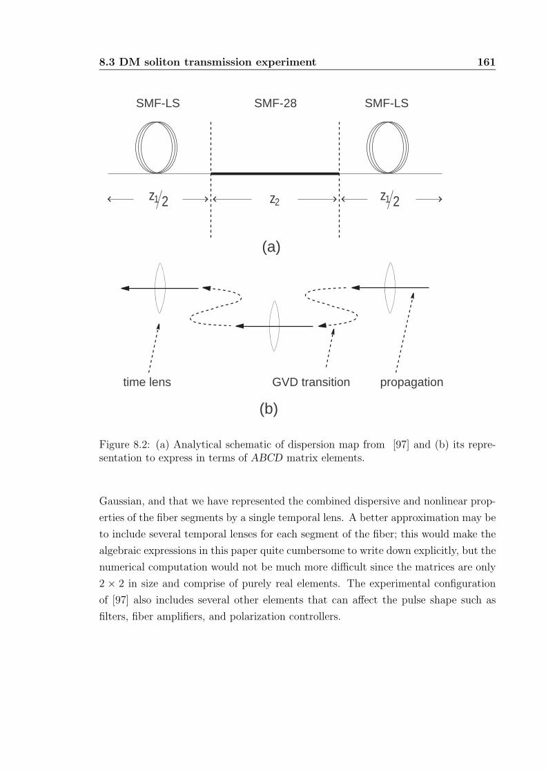
8.3 DM soliton transmission experiment 161
SMF-LS SMF-LSSMF-28
z1 2 z1 2z2
time lens GVD transition propagation
(a)
(b)
Figure 8.2: (a) Analytical schematic of dispersion map from [97] and (b) its repre-sentation to express in terms of ABCD matrix elements.
Gaussian, and that we have represented the combined dispersive and nonlinear prop-
erties of the fiber segments by a single temporal lens. A better approximation may be
to include several temporal lenses for each segment of the fiber; this would make the
algebraic expressions in this paper quite cumbersome to write down explicitly, but the
numerical computation would not be much more difficult since the matrices are only
2 × 2 in size and comprise of purely real elements. The experimental configuration
of [97] also includes several other elements that can affect the pulse shape such as
filters, fiber amplifiers, and polarization controllers.
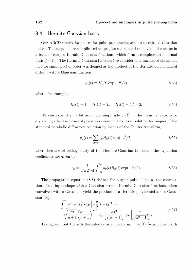
162 Space-time analogies in pulse propagation
8.4 Hermite-Gaussian basis
Our ABCD matrix formalism for pulse propagation applies to chirped Gaussian
pulses. To analyze more complicated shapes, we can expand the given pulse shape in
a basis of chirped Hermite-Gaussian functions, which form a complete orthonormal
basis [50, 73]. The Hermite-Gaussian function (we consider only unchirped Gaussians
here for simplicity) of order n is defined as the product of the Hermite polynomial of
order n with a Gaussian function,
ψn(t) ≡ Hn(t) exp(−t2/2), (8.53)
where, for example,
H0(t) = 1, H1(t) = 2t, H2(t) = 4t2 − 2. (8.54)
We can expand an arbitrary input amplitude u0(t) in this basis, analogous to
expanding a field in terms of plane wave components, as in solution techniques of the
standard parabolic diffraction equation by means of the Fourier transform,
u0(t) =∑n=0
cnHn(t) exp(−t2/2), (8.55)
where because of orthogonality of the Hermite-Gaussian functions, the expansion
coefficients are given by
cn =1√
π 2nn!
∫ ∞
−∞u0(t)Hn(t) exp(−t2/2). (8.56)
The propagation equation (8.8) defines the output pulse shape as the convolu-
tion of the input shape with a Gaussian kernel. Hermite-Gaussian functions, when
convolved with a Gaussian, yield the product of a Hermite polynomial and a Gaus-
sian [50], ∫ ∞
−∞dt0ψn(t0) exp
[−a
2(t − t0)
2]
=√2π
a + 1
(a − 1
a + 1
)n/2
exp
[a t2
2(a2 − 1)
]ψn
[a√
a2 − 1t
].
(8.57)
Taking as input the nth Hermite-Gaussian mode u0 = ψn(t) (which has width
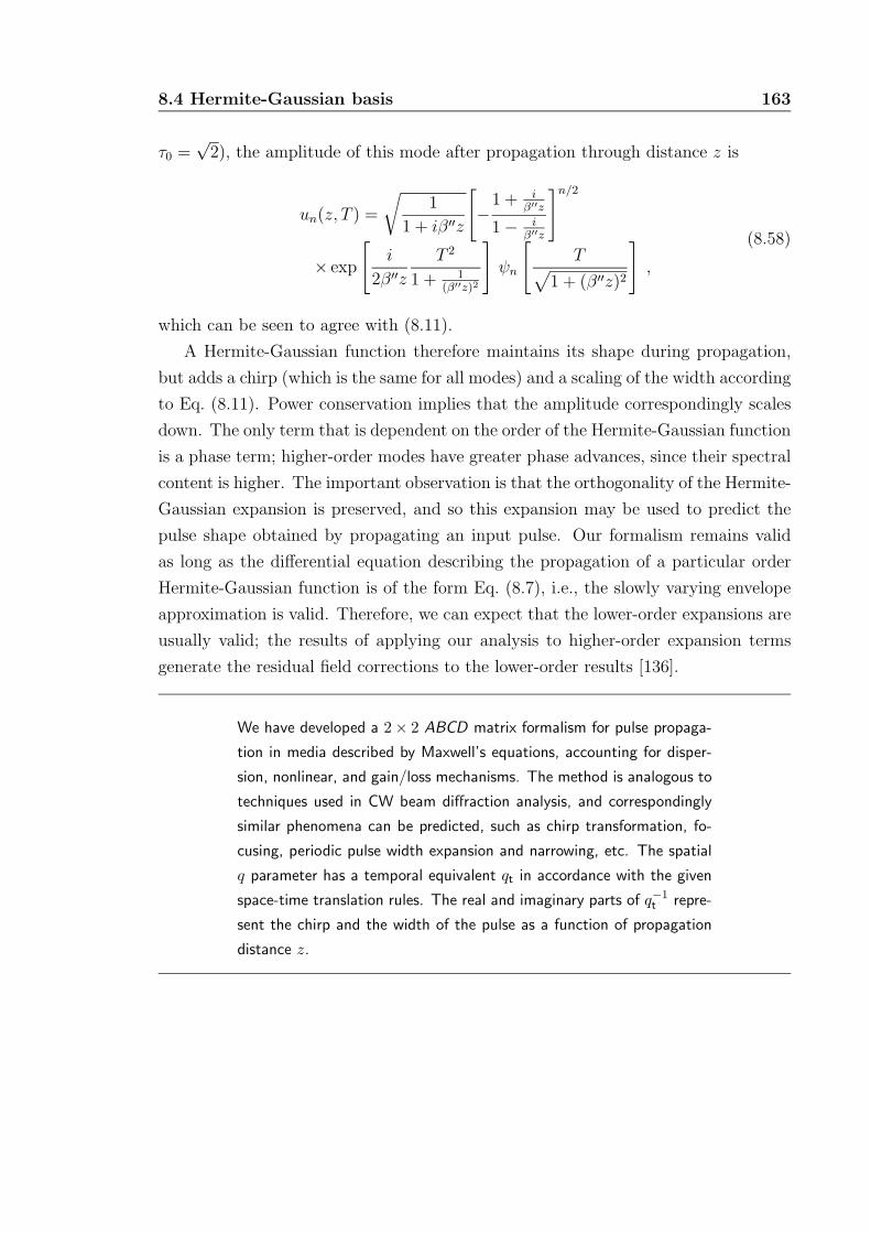
8.4 Hermite-Gaussian basis 163
τ0 =√
2), the amplitude of this mode after propagation through distance z is
un(z, T ) =
√1
1 + iβ′′z
[−1 + i
β′′z
1 − iβ′′z
]n/2
× exp
[i
2β′′zT 2
1 + 1(β′′z)2
]ψn
[T√
1 + (β′′z)2
],
(8.58)
which can be seen to agree with (8.11).
A Hermite-Gaussian function therefore maintains its shape during propagation,
but adds a chirp (which is the same for all modes) and a scaling of the width according
to Eq. (8.11). Power conservation implies that the amplitude correspondingly scales
down. The only term that is dependent on the order of the Hermite-Gaussian function
is a phase term; higher-order modes have greater phase advances, since their spectral
content is higher. The important observation is that the orthogonality of the Hermite-
Gaussian expansion is preserved, and so this expansion may be used to predict the
pulse shape obtained by propagating an input pulse. Our formalism remains valid
as long as the differential equation describing the propagation of a particular order
Hermite-Gaussian function is of the form Eq. (8.7), i.e., the slowly varying envelope
approximation is valid. Therefore, we can expect that the lower-order expansions are
usually valid; the results of applying our analysis to higher-order expansion terms
generate the residual field corrections to the lower-order results [136].
We have developed a 2 × 2 ABCD matrix formalism for pulse propaga-
tion in media described by Maxwell’s equations, accounting for disper-
sion, nonlinear, and gain/loss mechanisms. The method is analogous to
techniques used in CW beam diffraction analysis, and correspondingly
similar phenomena can be predicted, such as chirp transformation, fo-
cusing, periodic pulse width expansion and narrowing, etc. The spatial
q parameter has a temporal equivalent qt in accordance with the given
space-time translation rules. The real and imaginary parts of q−1t repre-
sent the chirp and the width of the pulse as a function of propagation
distance z.
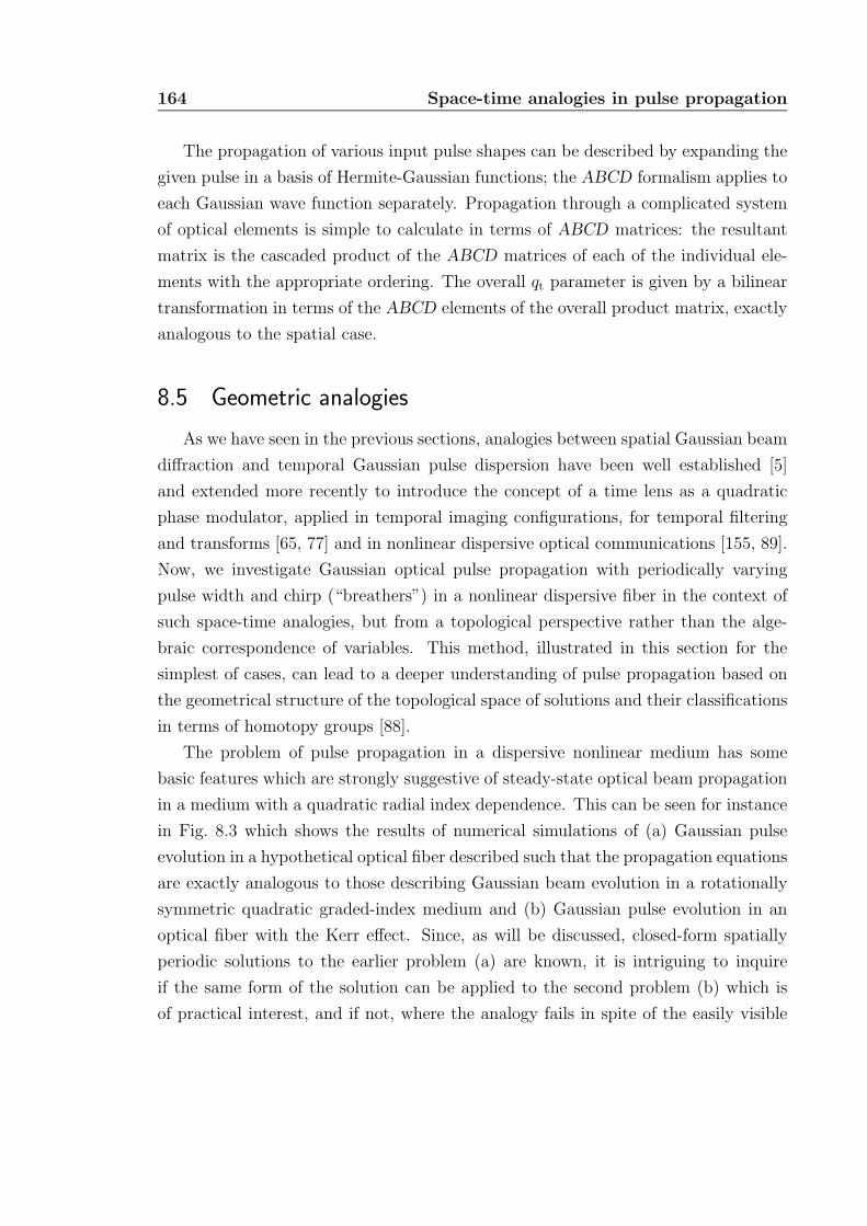
164 Space-time analogies in pulse propagation
The propagation of various input pulse shapes can be described by expanding the
given pulse in a basis of Hermite-Gaussian functions; the ABCD formalism applies to
each Gaussian wave function separately. Propagation through a complicated system
of optical elements is simple to calculate in terms of ABCD matrices: the resultant
matrix is the cascaded product of the ABCD matrices of each of the individual ele-
ments with the appropriate ordering. The overall qt parameter is given by a bilinear
transformation in terms of the ABCD elements of the overall product matrix, exactly
analogous to the spatial case.
8.5 Geometric analogies
As we have seen in the previous sections, analogies between spatial Gaussian beam
diffraction and temporal Gaussian pulse dispersion have been well established [5]
and extended more recently to introduce the concept of a time lens as a quadratic
phase modulator, applied in temporal imaging configurations, for temporal filtering
and transforms [65, 77] and in nonlinear dispersive optical communications [155, 89].
Now, we investigate Gaussian optical pulse propagation with periodically varying
pulse width and chirp (“breathers”) in a nonlinear dispersive fiber in the context of
such space-time analogies, but from a topological perspective rather than the alge-
braic correspondence of variables. This method, illustrated in this section for the
simplest of cases, can lead to a deeper understanding of pulse propagation based on
the geometrical structure of the topological space of solutions and their classifications
in terms of homotopy groups [88].
The problem of pulse propagation in a dispersive nonlinear medium has some
basic features which are strongly suggestive of steady-state optical beam propagation
in a medium with a quadratic radial index dependence. This can be seen for instance
in Fig. 8.3 which shows the results of numerical simulations of (a) Gaussian pulse
evolution in a hypothetical optical fiber described such that the propagation equations
are exactly analogous to those describing Gaussian beam evolution in a rotationally
symmetric quadratic graded-index medium and (b) Gaussian pulse evolution in an
optical fiber with the Kerr effect. Since, as will be discussed, closed-form spatially
periodic solutions to the earlier problem (a) are known, it is intriguing to inquire
if the same form of the solution can be applied to the second problem (b) which is
of practical interest, and if not, where the analogy fails in spite of the easily visible
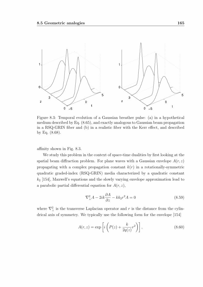
8.5 Geometric analogies 165
Figure 8.3: Temporal evolution of a Gaussian breather pulse: (a) in a hypotheticalmedium described by Eq. (8.65), and exactly analogous to Gaussian beam propagationin a RSQ-GRIN fiber and (b) in a realistic fiber with the Kerr effect, and describedby Eq. (8.68).
affinity shown in Fig. 8.3.
We study this problem in the context of space-time dualities by first looking at the
spatial beam diffraction problem. For plane waves with a Gaussian envelope A(r, z)
propagating with a complex propagation constant k(r) in a rotationally-symmetric
quadratic graded-index (RSQ-GRIN) media characterized by a quadratic constant
k2 [154], Maxwell’s equations and the slowly varying envelope approximation lead to
a parabolic partial differential equation for A(r, z),
∇2⊥A − 2ik
∂A
∂z− kk2r
2A = 0 (8.59)
where ∇2⊥ is the transverse Laplacian operator and r is the distance from the cylin-
drical axis of symmetry. We typically use the following form for the envelope [154]
A(r, z) = exp
[i
(P (z) +
k
2q(z)r2
)], (8.60)
166 Space-time analogies in pulse propagation
with the q-parameter1
q(z)≡ 1
R(z)− i
2λ
kw2(z)(8.61)
defined in terms of the the beam spot size w(z) and the radius of curvature of the
beam R(z). The solution q(z) for a given unchirped (R(0) = 0) input characterized
by q(0) = q0 is expressed in closed form by an ABCD bilinear transformation [154],
q(z) =A(z)q0 + B(z)
C(z)q0 + D(z), (8.62)
where
A(z) = cos
(√k2
kz
), B(z) =
√k
k2
sin
(√k2
kz
),
C(z) = −√
k2
ksin
(√k2
kz
), D(z) = cos
(√k2
kz
). (8.63)
This form of the solution clearly shows the breathing nature of the wave envelope,
i.e., periodic in width and in radius of curvature.
Next, in discussing temporal Gaussian pulse propagation, we know that group-
velocity dispersion (GVD) leads to broadening or narrowing of the temporal envelope
depending on the signs of the GVD parameter β′′ and chirp, although the shape
remains Gaussian. We may counteract this effect by utilizing self-phase modulation
(SPM) caused by a nonzero nonlinear-index coefficient n2. Breathers can be formed
when spectral broadening from a positive n2 balances anomalous dispersion (β′′ < 0)
in fibers. Similarly, negative n2 as found in AlGaAs waveguides [70] can compensate
the effect of normal dispersion, and breathers can be created in this case as well.
Self-consistent Gaussian breathers differ from conventional solitons [154] in that the
pulse parameters vary periodically in such a way that the pulse envelope can, by
assumption, always be described by a Gaussian function.
If SPM were to result in a (temporal) term analogous to the kk2r2 term in (8.59),
the solution would be temporally breathing Gaussian pulses similar to the spatial case
of breathing Gaussian beams, and this would satisfactorily explain the similarities of
Fig. 8.3: the solution would be given in closed form by the temporal equivalent of
8.5 Geometric analogies 167
Eq. (8.62), using the space-time translation rules tabulated in Table 8.1,
z → z, r → T, ∇2⊥ → ∇2
T , k → −1/β′′, k2 → 4γ, (8.64)
where T = t− z/vg is the temporal coordinate in the reference frame co-moving with
the pulse at the group velocity and γ = n2ω0/(cAeff) is the nonlinearity coefficient
defined in terms of the optical frequency ω0 and effective core area Aeff.
It is easily seen, however, that this is not the case. Applying the translation
rules (8.64) to Eq. (8.59) yields
−i∂A
∂z+
β′′
2
∂2A
∂T 2+
b2
2T 2A = 0, (8.65)
which we will refer to in this paper as the temporal RSQ-GRIN problem, whose
solution in obtainable in closed form using the ABCD form. But the wave equation
governing the propagation of the envelope of a Gaussian pulse in a nonlinear dispersive
fiber is [154]
−i∂A
∂z+
β′′
2
∂2A
∂T 2− γ
∆n
n2
A = 0, (8.66)
where n2 is the (constant) nonlinear index of refraction and ∆n(z, T ) is the Kerr
effect field-induced change in the refractive index. For a Gaussian pulse envelope of
width τ(z), ∆n can be approximated as
∆n(z, T ) = n2 exp
[−2
T 2
τ 2(z)
]≈ n2
[1 − 2T 2
τ 2(z)
], (8.67)
where we assume that the nonlinearity responds instantaneously. Eq. (8.66) becomes
−i∂A
∂z+
β′′
2
∂2A
∂T 2− γ
[1 − 2T 2
τ 2(z)
]A = 0. (8.68)
and clearly, Eqs. (8.68) and (8.65) are not identical. Therefore, the ABCD form of
the solution cannot apply to Eq. (8.68).
In order to explain the similarity shown in Fig. 8.3, we seek a different approach.
To identify analogies with the analysis of the spatial RSQ-GRIN problem Eq. (8.60),
168 Space-time analogies in pulse propagation
we write the temporal pulse Ansatz as
A(z, T ) = exp
[i
(P (z) +
T 2
2β′′q(z)
)], (8.69)
with a temporal q parameter,
1
q(z)≡ 1
R(z)+ i
2β′′
τ 2(z)
≡ r(z)[cos θ(z) + i sin θ(z)], (8.70)
where R(z) describes the chirp of the pulse and τ(z) its width. (We will use the
polar representation in our analysis later.) The chirped Gaussian envelope that this
formalism describes may, for instance, be one member of a complete orthonormal
basis of Hermite-Gaussian functions.
We can simplify each of the partial differential equations Eqs. (8.65) and (8.68) into
a pair of ordinary differential equations for P (z) and q(z) by substituting in for the
Ansatz given by Eq. (8.69) and then equating the coefficients of different powers of T .
We know from Gaussian beam diffraction analysis [154] that the equation with terms
quadratic in T involves only the initial-value problem for q(z). As q(z) is complex,
it is simplest to carry out a phase-plane analysis in each of the two systems in polar
(r, θ) co-ordinates using the definition presented in Eq. (8.70). In polar coordinates,
we can graph and compare the evolution of the solutions in the r − θ “phase” plane,
with z as the implicit variable driving the evolution of the instantaneous solution
along one of the contours in the phase plane.
The temporal RSQ-GRIN problem Eq. (8.65) in polar coordinates can be written
asdr/dz = r2 cos θ + 2γ cos θ,
dθ/dz =1
r
[r2 sin θ − 2γ sin θ
],
r(0) ≡ r0, θ(0) ≡ θ0 = π/2,
(8.71)
and for the equations describing pulse propagation in a nonlinear dispersive fiber
Eq. (8.68),
dr/dz = r2 cos θ + 2γ cos θ (r sin θ),
dθ/dz =1
r
[r2 sin θ − 2γ sin θ (r sin θ)
],
r(0) ≡ r0, θ(0) ≡ θ0 = π/2.
(8.72)
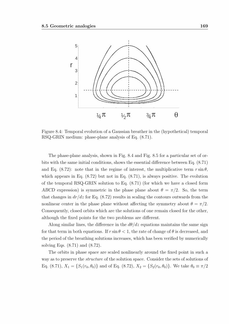
8.5 Geometric analogies 169
1
2
3
4
5
ππ π14 12
34
r
θ
Figure 8.4: Temporal evolution of a Gaussian breather in the (hypothetical) temporalRSQ-GRIN medium: phase-plane analysis of Eq. (8.71).
The phase-plane analysis, shown in Fig. 8.4 and Fig. 8.5 for a particular set of or-
bits with the same initial conditions, shows the essential difference between Eq. (8.71)
and Eq. (8.72): note that in the regime of interest, the multiplicative term r sin θ,
which appears in Eq. (8.72) but not in Eq. (8.71), is always positive. The evolution
of the temporal RSQ-GRIN solution to Eq. (8.71) (for which we have a closed form
ABCD expression) is symmetric in the phase plane about θ = π/2. So, the term
that changes in dr/dz for Eq. (8.72) results in scaling the contours outwards from the
nonlinear center in the phase plane without affecting the symmetry about θ = π/2.
Consequently, closed orbits which are the solutions of one remain closed for the other,
although the fixed points for the two problems are different.
Along similar lines, the difference in the dθ/dz equations maintains the same sign
for that term in both equations. If r sin θ < 1, the rate of change of θ is decreased, and
the period of the breathing solutions increases, which has been verified by numerically
solving Eqs. (8.71) and (8.72).
The orbits in phase space are scaled nonlinearly around the fixed point in such a
way as to preserve the structure of the solution space. Consider the sets of solutions of
Eq. (8.71), X1 = S1(r0, θ0) and of Eq. (8.72), X2 = S2(r0, θ0). We take θ0 ≡ π/2
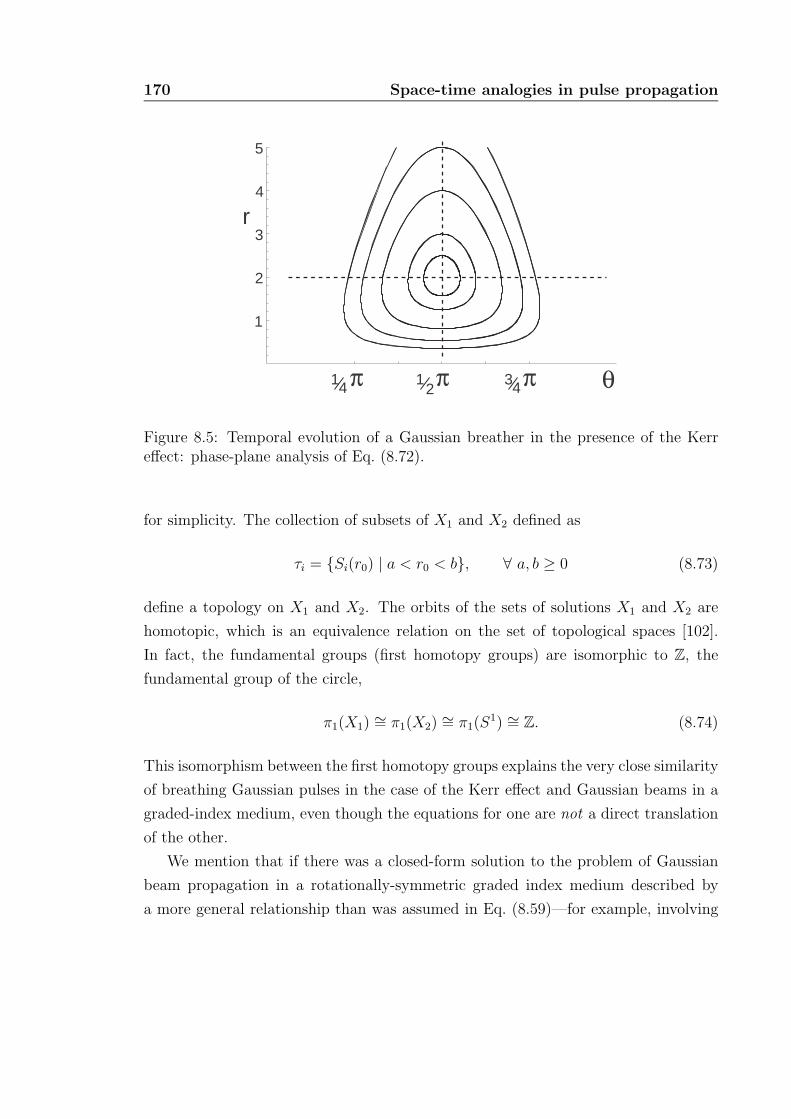
170 Space-time analogies in pulse propagation
1
2
3
4
5
ππ π14 12
34 θ
r
Figure 8.5: Temporal evolution of a Gaussian breather in the presence of the Kerreffect: phase-plane analysis of Eq. (8.72).
for simplicity. The collection of subsets of X1 and X2 defined as
τi = Si(r0) | a < r0 < b, ∀ a, b ≥ 0 (8.73)
define a topology on X1 and X2. The orbits of the sets of solutions X1 and X2 are
homotopic, which is an equivalence relation on the set of topological spaces [102].
In fact, the fundamental groups (first homotopy groups) are isomorphic to Z, the
fundamental group of the circle,
π1(X1) ∼= π1(X2) ∼= π1(S1) ∼= Z. (8.74)
This isomorphism between the first homotopy groups explains the very close similarity
of breathing Gaussian pulses in the case of the Kerr effect and Gaussian beams in a
graded-index medium, even though the equations for one are not a direct translation
of the other.
We mention that if there was a closed-form solution to the problem of Gaussian
beam propagation in a rotationally-symmetric graded index medium described by
a more general relationship than was assumed in Eq. (8.59)—for example, involving
8.5 Geometric analogies 171
higher powers of r2—then we could retain further terms in the Taylor series expansion
in Eq. (8.67) and apply the same topological arguments to justify the similarities of
the two families of solutions. The practical usefulness of such arguments depends,
however, on the existence of closed-form solutions in at least one of the two cases—
spatial or temporal—so that the solutions in the other case can be demonstrated to
be topologically equivalent or related. We expect that more such examples will be
identified in the future, leading to a deeper understanding of space-time analogies in
optical propagation.

172 Space-time analogies in pulse propagation
Epilogue
sreyan dravyamayad yajnaj jnanayajnah. paramtapasarvam karma ’khilam partha jnane parisamapyate
tad viddhi pran. ipatena pariprasnena sevayaupadeks.yanti te jnanam jnaninas tattvadarsinah.
—The Bhagavadgıta IV (33–34), S. Radhakrishnan ed., Blackie (1976).
173

174
Appendix A
Superstructure gratings
A grating in a semiconductor or an optical fiber is characterized by a periodic vari-
ation in the refractive index of the medium, typically in one dimension, e.g., n(z) =
n0 + ∆n(z) cos(2πz/d) where n0 is the average (“background”) refractive index, d is
the period of the grating and ∆n(z) is the amplitude of the index variation. The
simplest gratings are those for which ∆n(z) is a constant, e.g., ∆n(z) = ∆n0 for all z.
Superstructure gratings, (SSGs, or superstructure Bragg gratings, SBGs) are gratings
whose parameters in the description of ∆n(z) vary periodically along the length of
the grating [17, 35, 32], e.g., ∆n(z) = ∆n0 cos(2πz/Λ). Typically, the SSG period Λ
is much longer than d, the period of the underlying uniform grating, which is on the
scale of the wavelength of light. The reflection spectrum of weak gratings consists of a
peak at the Bragg frequency f = c/(2n0d) where n0 is the average refractive index in
the grating, surrounded by a comb of peaks at fk = c/2n0(1/d+k/Λ), k = ±1,±2, . . .
which are called Rowland ghosts. SSGs in semiconductor have been used in tunable
DFB lasers, and in optical fibers for dispersion compensation of WDM systems [17].
Using a coupled-mode theory with slowly varying envelopes, Broderick and de Sterke
have formulated equations describing propagation through a nonlinear SSG [17]. The
ansatz for the field envelope is
E(z, t) = a(z, t)Ψnk(z) e−iv∆nkt, (A.1)
where Ψnk is a Bloch function of the superstructure and ∆nk is the detuning from its
175
176 Superstructure gratings
corresponding eigenfrequency. The envelope1 a(z, t) is assumed to be slowly varying2
and if we consider only one band (i.e., only one Bloch function and its corresponding
envelope), it satisfies a nonlinear Schrodinger equation which has soliton solutions.
When two Bloch functions (and two envelopes) are considered in Eq. (A.1), the
single equation for a(z, t) becomes a pair of coupled mode equations for a1(z, t) and
a2(z, t) or equivalently, for a±(z, t) ≡ a1(z, t) ± a2(z, t), which are called “supercou-
pled mode equations” (SCMEs) by Broderick and de Sterke [17]3. For frequencies
sufficiently close to a Rowland ghost gap, these equations reduce to those describing
a shallow uniform nonlinear grating and therefore have soliton solutions (gap soli-
tons for a uniform grating, Rowland ghost solitons for an SSG in this regime) which
have been verified by numerical simulations [18] and experiments in optical fiber [35].
In addition to these bright soliton solutions, dark solitons and bright solitons on a
pedestal are also known [17].
A deep SSG is more appropriately described by the tight-binding method, as
was pointed out by de Sterke [32]. Such a grating can be though of as a periodic
array of regions with evanescent and propagating wave behavior, which is also seen in
the solutions to the simple quantum-mechanical problem of a periodic (square well)
potential [25]. In the weakly coupled regime, the eigenfield (waveguide mode) for an
SSG is written as a superposition of the eigenmodes of the individual wells, exactly
as in the description of a CROW [156]. It follows that our description of pulse
propagation in Chapter 2 and of second-harmonic generation in Chapter 3 can be
carried over to a deep SSG. It may easily be seen that the formulation of linear pulse
propagation in [92, MPEG movie] has many features in similar with the numerical
simulation of Rowland ghost solitons in a nonlinear SSG in [18, Fig. 4].
1Broderick and de Sterke refer to this as the “superenvelope” but since there is no other “enve-lope” in this formalism, we may simply refer to a(z, t) as the envelope (of the waveguide eigenmode).
2In space with respect to Γ, and in time with respect to (vκ0)−1 where κ0 is the lowest orderFourier component of κ(z) = π∆n(z)/λ.
3Again, there is nothing particularly “super” about this coupling, as physically the equationssimply describe the coupling of (eigen-) modes defined in a specific way; the particular form of theequations is dictated by the choice of the Ansatz.
Appendix B
Watson’s criterion and Gaussian envelopes
As discussed by Watson [145, pp. 533–535], there are three criteria that need to be
satisfied by an odd function f(x) in order for the expansion Eq. (2.50) to be valid.
In our case, f(x) is related (by a linear transformation) to the envelope of the pulse
at the z = 0 cross-section of the CROW, and it is entirely reasonable to assume that
1.∫∞
0f(x)dx exits and is absolutely convergent.
In our analysis, the most important class of functions that represent pulse envelopes
are Gaussians (of real arguments) and we may assume that
2. f(x′) has a continuous differential coefficient for all positive values of x′ <
x, where x refers to the particular value of x chosen in the left hand side of
Eq. (2.50).
Watson’s third criterion is in the form of an integral equation,
3. For all t < x,
2f ′(t) =
∫ ∞
0
dv
vJ1(v) [f(v + t) + f(v − t)] . (B.1)
We do not need to rigorously analyze this condition, and will appeal instead to
physical arguments. We assume that the envelopes we consider [such as taking the
form of Eq. (2.52)] are sufficiently well behaved so that, using the definition of a
derivative,
f ′(t) =1
2limv→0
[f(t + v) − f(t)
v+
f(t) − f(t − v)
v
], (B.2)
and since f(t) is odd,
2f ′(t) = limv→0
f(v + t) + f(v − t)
v. (B.3)
177
178 Watson’s criterion and Gaussian envelopes
It is now evident that one simple way of approximately satisfying Eq. (B.1) is to
stipulate f(t + v) ≈ f(t − v), and in the limit of equality of the last relationship,
the former is satisfied exactly (and trivially). In the context of Eq. (2.52), broader
Gaussian envelopes, with larger T , are “better” represented by the Webb-Kapteyn-
Neumann series. This is easily verified numerically.
More detailed investigations of Eq. (B.1) in the context of Eq. (2.52) are un-
likely, we believe, to reveal much more useful information. A criterion established by
Bateman [10] for the validity of Eq. (2.50) is
∫ ∞
0
dt f(t) J0(tx) =
ψ(x), if x < 1,
0, otherwise,(B.4)
where ψ(x) is a function that takes nonzero values only on the interval 0 < x < 1.
Using Eq. (2.52) for f(t),
∫ ∞
0
dt e−t2
T2 J0(tx) =
√π T
2e−T 2x2/8I0
(T 2x2
8
)
∼ 1
xas x → ∞,
(B.5)
and Eq. (B.4) is clearly not satisfied for any value of T . Nevertheless, Gaussian en-
velopes [and others with a property similar to Eq. (B.5)] are of considerable interest
practically. In this context, the approach we have taken in the previous paragraph
circumvents the assumptions underlying Eq. (B.4) and Bateman’s subsequent conclu-
sions.
Appendix C
Outline of the proof of the Hermiticity of H
Using the two vector identities,
∇ · (a × b) = b · (∇× a) − a · (∇× b),
a · (b × c) = −(b × a) · c, (C.1)
it is easy to show that the the operator H defined in Eq. (2.38) is Hermitian, provided
that the boundary conditions are of the appropriate form [96]. To show this explicitly
for each of the 6 component terms of H as written in Eq. (2.38) is needlessly tedious,
as all the neccessary operations can be demonstrated by considering terms 3 and 4 of
H. We will therefore show that the operator H ′, which is defined by
H ′uk(ω) ≡ −ik[∇× [ez × uk(ω)] + ez × [∇× uk(ω)]
], (C.2)
is Hermitian, i.e., satisfies the following equality among inner products,
(uk(ω), H′uk(ω)) = (H ′uk(ω),uk(ω)), (C.3)
with the inner product definition following Eq. (2.36). The full operator H can be
checked in a similar way.
If the following boundary condition holds,
∫dt
T
∫dr ε(r)∇ · [(∇× uk(ω)) × u∗
k(ω)
]= 0, (C.4)
where the region of r integration is over a unit cell and the region of t integration is
179
180 Outline of the proof of the Hermiticity of H
over the temporal extent of the envelope, then using Eq. (C.1),
(uk(ω), H′uk(ω)) =
∫dt
T
∫dr [−ik ε(r)]
[(∇ · uk(ω))
∗ · [ez × uk(ω)]
−(ez × uk(ω))∗ · (∇× uk(ω))
]=
∫dt
T
∫dr [−ik ε(r)]
[− (
ez × [∇× uk(ω)])∗ · uk(ω)
− (∇× [ez × uk(ω)])∗ · uk(ω)
= (H ′uk(ω),uk(ω)). (C.5)
For terms 5 and 6 of H as given by Eq. (2.38), the following boundary condition
is needed: ∫dr ε(r)
[[uk(ω)
]∗ · (ε(r)
c2
∂uk(ω)
∂t
)∣∣∣∣t+
t−
]= 0. (C.6)
Eqs. (C.4) and (C.6) are satisfied physically since the CROW is a spatially periodic
structure and the pulse envelope goes to zero at both ends of the t integration.
Such boundary conditions are a mathematical statement of the assumption that
the problem of interest is physically completely contained in the CROW. Problems
of coupling a pulse into or out of a CROW of finite length cannot be described by
Hermitian eigenvalue equations as the bilinear concommitant between the original
differential equation and its Hermitian adjoint is no longer periodic [96]. In such
circumstances, one can resort to direct numerical methods of analysis [149].
The imposition of closed boundary conditions in the temporal domain is for sim-
plicity. A more correct approach would allow the positive temporal boundary to
go to infinity and impose appropriate Cauchy boundary conditions (value and slope
specified) on the wave equation. Whereas Cauchy boundary conditions overspecify a
closed boundary hyperbolic differential equation, they provide for a unique and stable
solution to the open boundary problem [96].
Appendix D
Nonlinear polarization for SHG
Based on the discussion of the waveguide modes of a CROW in Chapters 2 and 3, we
assume the following forms for two eigenfields at the fundamental frequency ω with
amplitudes E1,
Ea(r, t) = E1 eiωte−ik1(ω)zuk1(ω)(r, t), (D.1)
Eb(r, t) = E1 eiωte−ik2(ω)zuk2(ω)(r, t). (D.2)
For each field, the frequency-domain (temporal Fourier transformed) field can be
written as
E(r, Ω) ≡ E1
∫dt e−iΩtE(r, t)
= E1 e−ik1(ω)zuk1(r, Ω), (D.3)
where we use the tilde to represent Fourier transformed fields.
The frequency-domain nonlinear polarization for second harmonic generation at
ω2 is given by [154, 126]
PNL(r, ω2) = d(r)
∫ ∞
−∞dΩ Ea(r, ω2 − Ω)Eb(r, Ω), (D.4)
where d is the effective second-order nonlinearity coefficient of the medium. Using
181
182 Nonlinear polarization for SHG
Eq. (D.3), Eq. (D.4) can be written as
PNL(r, ω2) = d(r)E21
∫ ∞
−∞dΩ e−i[k1(ω2−Ω)+k2(Ω)]z
× uk1(r, ω2 − Ω − ω) uk2(r, Ω − ω).
(D.5)
The dispersion relationship between k and ω implies that we can expand k(ω) in
a Taylor series about the central frequency of each pulse [154]. We retain terms upto
the linear in ω to write
k1(ω2 − Ω) = k1 +dk
dω
∣∣∣∣ω
(ω2 − Ω − ω),
k2(Ω) = k2 +dk
dω
∣∣∣∣ω
(Ω − ω). (D.6)
The group velocity at ω1 is defined by the relation 1/v1 = (dk/dω)|ω1 . The assumption
of a linear dispersion relationship in a CROW is not as restrictive as one might expect
based on ω-K curves for conventional waveguides. From the tight-binding analysis,
the dispersion relationship for a weakly coupled CROW can be written as
ω(k) = Ω
[1 − ∆α
2+ κ cos(kR)
](D.7)
where Ω is the mode frequency of the individual resonators, ∆α is an overlap integral
and κ is a coupling coefficient. The group velocity dω/dk goes to zero at the edges of
the Brillouin zone k = 0,±π/R1, but is approximately constant in the central portion
of the zone, where the dispersion relationship is linear.
We can use Eq. (D.6) in Eq. (D.5) and take the inverse Fourier transform to write
the nonlinear polarization in the time domain,
PNL(r, t) =
∫dω2
2πeiω2t PNL(r, ω2)
1Consequently, there are no linear propagating eigenmodes at these points, and referring to thevarious waveguide modes as “states,” we can say that the density of states is zero. In the solid-statephysics of electron levels, these points are known as van Hove singularities [9].
183
or when written out completely,
PNL(r, t) = d(r) E12e−i(k1−ω/v1)ze−i(k2−ω/v1)z
×∫
dω2
2πeiω2(t−z/v1)
∫ ∞
−∞dΩ
[uk1(r, ω2 − Ω − ω) uk2(r, Ω − ω)
]
= d(r) E12[ei(ωt−k1z)uk1(ω)(r, t − z/v1)
][ei(ωt−k2z)uk2(ω)(r, t − z/v1)
].
(D.8)
This can be easily generalized to include a spatial and temporal dependency in
the envelope E1. We can simply include the non-constant part of E1 with the spatial
and temporally varying function uk(ω)(r, t) as the physical interpretation of uk(ω) as
a Bloch wavefunction is irrelevant here. The result is
PNL(r, t) =d(r)[Ea(z) ei(ωt−k1z)uk1(ω)(r, t − z/v1)
][Eb(z)ei(ωt−k2z)uk2(ω)(r, t − z/v1)
].
(D.9)
For simplicity, we will usually assume that the envelopes Ea and Eb are constant
= E1, signifying an undepleted eigenmode at the fundamental carrier frequency ω.

184 Nonlinear polarization for SHG
Appendix E
Period of orbits in the phase plane
Rather than work with the direct form of the Hamiltonian, Eq. (6.10), we introduce
the following change of variables: β = β/π, Z = Z(π/2), and then drop the bars for
notational simplicity. Writing H ′ = −2/3 H and assuming that a(Z) ≡ 1 we obtain
H ′ = (σ + 6γΩ)
[β2
η2+ η2 + Ω2
]− 2(η − Ω2σ) (E.1)
and Eq. (6.12) becomes
dη
dz= −(σ + 6γΩ)βη, (E.2)
dβ
dz= (σ + 6γΩ)(η4 − β2) − η3. (E.3)
For a given level set of this redefined Hamiltonian, parametrized by H ′, Eq. (E.1)
is of quadratic order in β, so that
β = ±η
√H ′ + 2(η − Ω2σ)
σ + 6γΩ− (η2 + Ω2). (E.4)
Since dΩ/dz = 0, and both σ and γ are assumed to be piecewise constant, we can
use Eq. (E.2) to find the distance Z2 − Z1 between the points η = η2 and η1 on the
H ′ contour,
∫ η2
η1
dη
±η2
√H ′ + 2(η − Ω2σ)
σ + 6γΩ− (η2 + Ω2)
−1
= −(Z2 − Z1)(σ + 6γΩ). (E.5)
185
186 Period of orbits in the phase plane
Identifying a = (H ′ − 2Ω2σ)/(σ + 6γΩ) − Ω2, b = 2/(σ + 6γΩ), and c = −1, we
can use the following identity to evaluate the integral,
∫dx
x2√
a + bx + cx2= −
√a + bx + cx2
ax+
b
2a3/2log
[− 2
bx
(2a3/2 +
√a b x
+ 2a√
a + bx + cx2)]
.
(E.6)
We now take η1 and η2 to correspond to the minimum and maximum extents of
the orbit along the η axis (see Fig. 1). These two points are given by the solutions of
the following algebraic equation,
η2 − 2
σ + 6γΩ+
(Ω2 − H ′ − 2Ω2σ
σ + 6γΩ
)= 0. (E.7)
The round-trip period of the H ′ orbit is given by the value of 2(Z2 − Z1), obtained
from Eq. (E.5).
Based on Eq. (E.4), we can solve dβ/dη = 0 to find the η value corresponding
that point on the orbit where β is maximum,
η|βmax=
3
4(σ + 6γΩ)+
1
2
√9
4(σ + 6γΩ)2+
2(E − 3σΩ2 − 6γΩ3)
σ + 6γΩ. (E.8)
Using this value for η in Eq. (E.4) leads to a value for βmax.
References
[1] M. A. Abramowitz and I. A. Stegun. Handbook of Mathematical Functions. Dover, 1972.
[2] A. Adibi, Y. Xu, R. K. Lee, A. Yariv, and A. Scherer. Properties of the slab modes in photoniccrystal optical waveguides. Journal of Lightwave Technology, 18(11):1554–1564, 2000.
[3] G. P. Agrawal. Fiber-Optic Communication Systems. John Wiley & Sons, second edition,1997.
[4] G.P. Agrawal. Nonlinear Fiber Optics. Academic Press, 1989.
[5] S. A. Akhmanov, A. S. Chirkin, K. N. Drabovich, A. I. Kovrigin, R. V. Khokhlov, and A.P.Sukhorukov. Nonstationary nonlinear optical effects and ultrashort light pulse pulse formation.IEEE Journal of Quantum Electronics, QE-4(10):598, 1968.
[6] N. Akhmediev and M. Karlsson. Cherenkov radiation emited by solitons in optical fibers.Physical Review A, 51(3):2602–2607, 1995.
[7] D. Anderson. Variational approach to nonlinear pulse propagation in optical fibers. Phys.Rev. A, 27:3135–3145, 1983.
[8] T. M. Apostol. Mathematical Analysis. Addison-Wesley, 1957.
[9] N. W. Ashcroft and N. D. Mermin. Solid State Physics. Harcourt, Fort Worth, 1976.
[10] H. Bateman. On an expansion of an arbitrary function in a series of Bessel functions. TheMessenger of Mathematics, XXXVI:31–37, 1907.
[11] M. Bayer, I. Gutbrod, A. Forchel, T. Reinecke, P. Knipp, R. Werner, and J. Reithmaier.Optical demonstration of a crystal band structure formation. Physical Review Letters, 83:5374,1999.
[12] M. Bayer, I. Gutbrod, J. P. Reithmaier, A. Forchel, T. L. Reinecke, P. A. Knipp, A. A.Dremin, and Kulakovskii V. D. Optical modes in photonic molecules. Physical Review Letters,81(12):2582–2585, 1998.
[13] M. Bayindir, B. Temelkuran, and E. Ozbay. Tight-binding description of the coupled defectmodes in three-dimensional photonic crystals. Physical Review Letters, 84(10):2140–2143,2000.
187
188 References
[14] P. A. Belanger and P. Mathieu. On an extremum property of Gaussian beams and Gaussianpulses. Optics Communications, 67(6):396–398, 1988.
[15] A. Bondeson, M. Lisak, and D. Anderson. Soliton perturbations: a variational principle forthe soliton parameters. Physica Scripta, 20:479–485, 1979.
[16] M Born and E. Wolf. Principles of Optics. Cambridge University Press, seventh edition, 1999.
[17] N. G. R. Broderick and C. M. de Sterke. Theory of grating superstructures. Physical ReviewE, 55(3):3634–3647, 1997.
[18] N. G. R. Broderick, C. M. de Sterke, and B. J. Eggleton. Soliton solutions in Rowland ghostgaps. Physical Review E, 52(6):R5788–R5791, 1995.
[19] K. Busch and S. John. Liquid-crystal photonic band-gap materials: The tunable electromag-netic vacuum. Physical Review Letters, 83(5):967–970, 1999.
[20] E. Caglioti, B. Crosignani, and P. Di Porto. Hamiltonian description of nonlinear propagationin optical fibers. Physical Review A, 38(8):4036–4042, 1988.
[21] E. Caglioti, S. Trillo, S. Wabnitz, B. Crosignani, and P. Di Porto. Finite-dimensional de-scription of nonlinear pulse propagation in optical-fiber couplers with applications to solitonswitching. Journal of the Optical Society of America B, 7(3):374–385, 1990.
[22] G. M. Carter, R.-M. Mu, V. S. Grigoryan, C. R. Menyuk, P. Sinha, F. Carruthers, M. L.Dennis, and I. N. Duling III. Transmission of disperion-managed solitons at 20 Gbits/s over20 000 km. Electronics Letters, 35:133–134, 1999.
[23] E. Chow, S. Y. Lin, S. G. Johnson, P. R. Villeneuve, J. D. Joannopoulos, J. R. Wendt, G. A.Vawter, W. Zubrzycki, H. Hou, and A. Alleman. Three-dimensional control of light in atwo-dimensional photonic crystal slab. Nature, 407:983–986, 2000.
[24] D. N. Christodoulides and N. K. Efremidis. Discrete temporal solitons along a chain of non-linear coupled microcavities embedded in photonic crystals. Optics Letters, 27(8):568–570,2002.
[25] C. Cohen-Tannoudji, B. Diu, and F. Laloe. Quantum Mechanics. Hermann and John Wiley& Sons, 1977.
[26] C. Cohen-Tannoudji, J. Dupont-Roc, and G. Grynberg. Photons and Atoms. John Wiley &Sons, New York, 1989.
[27] C. Conti, S. Trillo, and G. Assanto. Energy localization in photonic crystals of a purelynonlinear origin. Physical Review Letters, 85:2502–2505, 2000.
[28] B. Crosignani. Nonlinear effects in optical fibers. Fiber and Integrated Optics, 11:235–252,1992.
[29] B. Crosignani, P. Di Porto, and E. Caglioti. The optical Kerr effect in fibers. In A.R. Board-man, M. Bertolotti, and T. Twardowski, editors, Nonlinear Waves in Solid State Physics,NATO ASI Series B. Vol. 247. Plenum Press, 1990.
References 189
[30] W. B. Davenport and W. L. Root. An Introduction to the Theory of Random Signals andNoise. McGraw-Hill, New York, 1958.
[31] C. J. S. de Matos, D. A. Chestnut, and J. R. Taylor. Wavelength- and duration-tunablesoliton source based on a 20-GHz Mach-Zehnder modulator and adiabatic Raman compression.Applied Physics Letters, 81:2932–2934, 2002.
[32] C. M. de Sterke. Superstructure gratings in the tight-binding approximation. Physical ReviewE, 57(3):3502–3509, 1998.
[33] E. Desurvire, M. Zirngibl, H. M. Presby, and D. DiGiovanni. Characterization and modeling ofamplified spontaneous emission in unsaturated erbium-doped fiber amplifiers. IEEE PhotonicsTechnology Letters, 3:127–129, 1991.
[34] J. P. Dowling, M. Scalora, M. J. Bloemer, and C. M. Bowden. The photonic band edge laser:a new approach to gain enhancement. Journal of Applied Physics, 75:1896–1899, 1994.
[35] B. J. Eggleton, C. M. de Sterke, and R. E. Slusher. Nonlinear propagation in superstructureBragg gratings. Optics Letters, 21(16):1223–1225, 1996.
[36] A. Erdelyi, editor. Higher Transcendental Functions, volume II. McGraw-Hill, 1953.
[37] R. P. Feynman. Forces in molecules. Physical Review, 56:340–343, 1939.
[38] H. Ghafouri-Shiraz, P. Shum, and M. Nagata. A novel method for analysis of soliton propa-gation in optical fibers. IEEE Journal of Quantum Electronics, 31(1):190–200, 1995.
[39] H. Goldstein. Classical Mechanics. Addison-Wesley, 1950.
[40] J.P. Gordon. Theory of the soliton self-frequency shift. Optics Letters, 11(10):662–664, 1986.
[41] J.P. Gordon. Dispersive perturbations of solitons of the nonlinear schrodinger equation. Jour-nal of the Optical Society of America B, 9:91–97, 1992.
[42] J.P. Gordon and H.A. Haus. Random walk of coherently amplified solitons in optical fibertransmission. Optics Letters, 11(10):665–667, 1986.
[43] A. Hasegawa. Soliton-based optical communications: an overview. IEEE Journal of SelectedTopics in Quantum Electronics, 6(6):1161–1172, 2000.
[44] A. Hasegawa and Y. Kodama. Solitons in Optical Communications. Oxford, 1995.
[45] A. Hasegawa and T. Nyu. Eigenvalue communication. Journal of Lightwave Technology,11(3):395–399, 1993.
[46] H. Hatami-Hanza, J. Hong, A. Atieh, P. Mylinski, and J. Chrotowski. Demonstration ofall-optical demultiplexing of a multilevel soliton signal employing soliton decomposition andself-frequency shift. IEEE Photonics Technology Letters, 9(6):833–835, 1997.
[47] H. A. Haus. Optical fiber solitons, their propertes and uses. Proceedings of the IEEE,81(7):970–983, 1993.
190 References
[48] H. A. Haus and M. N. Islam. Theory of the soliton laser. IEEE Journal of Quantum Electronics,QE-21(8):1172–1188, 1985.
[49] H. A. Haus, K. Tamura, L. Nelson, and E. P. Ippen. Stretched-pulse additive pulse mode-locking in fiber ring lasers: Theory and experiment. IEEE Journal of Quantum Electronics,31(2):591–598, 1995.
[50] H.A. Haus. Waves and Fields in Optoelectronics. Prentice-Hall, 1984.
[51] H.A. Haus and W.S. Wong. Solitons in optical communications. Reviews of Modern Physics,68(2):423–444, 1996.
[52] H. Hellman. Einfurung in die Quantenchemie. Deuticke, 1937.
[53] R. Hirota. Exact envelope-soliton solutions of a nonlinear wave equation. Journal of Mathe-matical Physics, 14(7):805–809, 1973.
[54] P. Holmes and J.N. Kutz. Dynamics and bifurcations of a planar map modeling dispersionmanaged breathers. SIAM J. Appl. Math, 59(4):1288–1302, 1999.
[55] E. Infeld and G. Rowlands. Nonlinear Waves, Solitons and Chaos. Cambridge UniversityPress, second edition, 2000.
[56] T. Inoue, H. Suguhara, A. Maruta, and Y. Kodama. Interactions between dispersion-managedsolitons in optical time-division-multiplexed system. IEEE Photonics Technology Letters,12(3):299–301, 2000.
[57] J. D. Jackson. Classical Electrodynamics. John Wiley & Sons, third edition, 1999.
[58] J. D. Joannopoulos, R. D. Meade, and J. N. Winn. Photonic Crystals. Princeton UniversityPress, 1995.
[59] S. John and N. Akozbek. Nonlinear optical solitary waves in a photonic band-gap. PhysicalReview Letters, 71(8):1168–1171, 1993.
[60] S. G. Johnson and J. D. Joannopoulos. Block-iterative frequency-domain methods formaxwell’s equations in a planewave basis. Optics Express, 8:173–190, 2001.
[61] S. G. Johnson, P. R. Villeneuve, S. Fan, and J. D. Joannopoulos. Linear waveguides inphotonic-crystal slabs. Physical Review B, 62(12):8212–8222, 2000.
[62] H. Jones. The Theory of Brillouin Zones and Electronic States in Crystals. North-Holland,1960.
[63] V. I. Karpman. Soliton evolution in the presence of perturbations. Physica Scripta, 20:462–478,1979.
[64] Y. S. Kivshar and D. E. Pelinovsky. Self-focusing and transverse instabilities of solitary waves.Physics Reports, 331:117–195, 2000.
[65] B. H. Kolner and M. Nazarathy. Temporal imaging with a time lens. Optics Letters, 14(12):630,1989.
References 191
[66] S. Kumar and F. Lederer. Gordon-Haus effect in dispersion-managed soliton systems. OpticsLetters, 22(24):1870–1872, 1997.
[67] J. Kumasako, M. Matsumoto, and S. Waiyapot. Linear stability analysis of dispersion-managedsolitons controlled by filters. Journal of Lightwave Technology, 18(8):1064–1068, 2000.
[68] J.N. Kutz, P. Holmes, S.G. Evangelides, and J.P. Gordon. Hamiltonian dynamics of dispersionmanaged breathers. J. Opt. Soc. Am. B, 15(1):87–96, 1998.
[69] J.N. Kutz and P.K.A. Wai. Noise-induced amplitude and chirp jitter in dispersion-managedsoliton communications. Optics Letters, 23(13):1022–1024, 1998.
[70] M. J. LaGasse, K. K. Anderson, C. A. Wang, H. A. Haus, and J. G. Fujimoto. Femtosec-ond measurements of the nonresonant nonlinear index in AlGaAs. Applied Physics Letters,56(5):417–419, 1990.
[71] T. I. Lakoba. Non-integrability of equations governing pulse propagation in dispersion-managed optical fibers. Physics Letters A, 260:68–77, 1999.
[72] T. I. Lakoba and G. P. Agrawal. Effects of third-order dispersion on dispersion-managedsolitons. Journal of the Optical Society of America B, 16(9):1332–1343, 1999.
[73] T. I. Lakoba and D. J. Kaup. Hermite-gaussian expansion for pulse propagation in stronglydispersion managed fibers. Physical Review E, 58(5):6728–6741, November 1998.
[74] R. J. Lang and A. Yariv. Analysis of the dynamic response of multielement semiconductorlasers. IEEE Journal of Quantum Electronics, QE-21(10):1683–1688, 1985.
[75] R. J. Lang and A. Yariv. Local-field rate equations for coupled optical resonators. PhysicalReview A, 34(3):2038–2043, 1986.
[76] G. Lehmann and P. Ziesche. Electronic Properties of Metals, volume 64 of Materials ScienceMonographs. Elsevier, 1990.
[77] A. W. Lohmann and D. Mendlovic. Temporal filtering with time lenses. Applied Optics,31(9):6212, 1992.
[78] M. Loncar, D. Nedeljkovic, T. Doll, J. Vuckovic, A. Scherer, and T.P. Pearsall. Waveguidingin planar photonic crystals. Applied Physics Letters, 77(13):1937–1939, 2000.
[79] R. Loudon. The Quantum Theory of Light. Oxford, second edition, 1997.
[80] R. S. Mackay and S. Aubry. Proof of existence of breathers for time-reversible or Hamiltoniannetworks of weakly coupled oscillators. Nonlinearity, 7(6):1623–1643, 1994.
[81] D. Marcure and C. R. Menyuk. Simulation of single-channel optical systems at 100 Gb/s.Journal of Lightwave Technology, 17(4):564–569, 1999.
[82] D. Marcuse. An alternative derivation of the Gordon-Haus effect. Journal of LightwaveTechnology, 10(2):273–278, 1992.
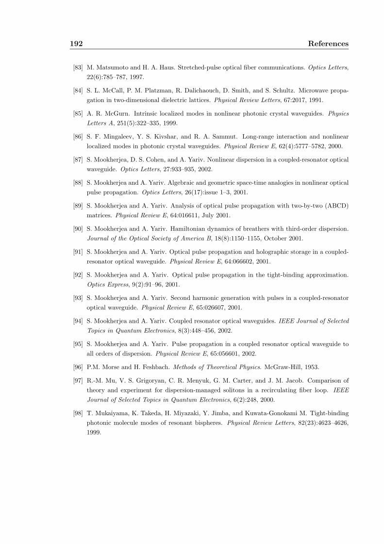
192 References
[83] M. Matsumoto and H. A. Haus. Stretched-pulse optical fiber communications. Optics Letters,22(6):785–787, 1997.
[84] S. L. McCall, P. M. Platzman, R. Dalichaouch, D. Smith, and S. Schultz. Microwave propa-gation in two-dimensional dielectric lattices. Physical Review Letters, 67:2017, 1991.
[85] A. R. McGurn. Intrinsic localized modes in nonlinear photonic crystal waveguides. PhysicsLetters A, 251(5):322–335, 1999.
[86] S. F. Mingaleev, Y. S. Kivshar, and R. A. Sammut. Long-range interaction and nonlinearlocalized modes in photonic crystal waveguides. Physical Review E, 62(4):5777–5782, 2000.
[87] S. Mookherjea, D. S. Cohen, and A. Yariv. Nonlinear dispersion in a coupled-resonator opticalwaveguide. Optics Letters, 27:933–935, 2002.
[88] S. Mookherjea and A. Yariv. Algebraic and geometric space-time analogies in nonlinear opticalpulse propagation. Optics Letters, 26(17):issue 1–3, 2001.
[89] S. Mookherjea and A. Yariv. Analysis of optical pulse propagation with two-by-two (ABCD)matrices. Physical Review E, 64:016611, July 2001.
[90] S. Mookherjea and A. Yariv. Hamiltonian dynamics of breathers with third-order dispersion.Journal of the Optical Society of America B, 18(8):1150–1155, October 2001.
[91] S. Mookherjea and A. Yariv. Optical pulse propagation and holographic storage in a coupled-resonator optical waveguide. Physical Review E, 64:066602, 2001.
[92] S. Mookherjea and A. Yariv. Optical pulse propagation in the tight-binding approximation.Optics Express, 9(2):91–96, 2001.
[93] S. Mookherjea and A. Yariv. Second harmonic generation with pulses in a coupled-resonatoroptical waveguide. Physical Review E, 65:026607, 2001.
[94] S. Mookherjea and A. Yariv. Coupled resonator optical waveguides. IEEE Journal of SelectedTopics in Quantum Electronics, 8(3):448–456, 2002.
[95] S. Mookherjea and A. Yariv. Pulse propagation in a coupled resonator optical waveguide toall orders of dispersion. Physical Review E, 65:056601, 2002.
[96] P.M. Morse and H. Feshbach. Methods of Theoretical Physics. McGraw-Hill, 1953.
[97] R.-M. Mu, V. S. Grigoryan, C. R. Menyuk, G. M. Carter, and J. M. Jacob. Comparison oftheory and experiment for dispersion-managed solitons in a recirculating fiber loop. IEEEJournal of Selected Topics in Quantum Electronics, 6(2):248, 2000.
[98] T. Mukaiyama, K. Takeda, H. Miyazaki, Y. Jimba, and Kuwata-Gonokami M. Tight-bindingphotonic molecule modes of resonant bispheres. Physical Review Letters, 82(23):4623–4626,1999.
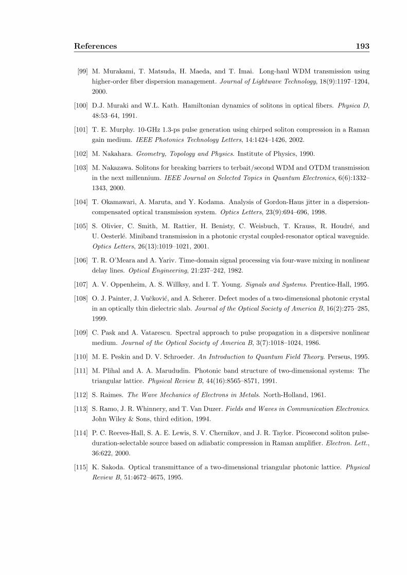
References 193
[99] M. Murakami, T. Matsuda, H. Maeda, and T. Imai. Long-haul WDM transmission usinghigher-order fiber dispersion management. Journal of Lightwave Technology, 18(9):1197–1204,2000.
[100] D.J. Muraki and W.L. Kath. Hamiltonian dynamics of solitons in optical fibers. Physica D,48:53–64, 1991.
[101] T. E. Murphy. 10-GHz 1.3-ps pulse generation using chirped soliton compression in a Ramangain medium. IEEE Photonics Technology Letters, 14:1424–1426, 2002.
[102] M. Nakahara. Geometry, Topology and Physics. Institute of Physics, 1990.
[103] M. Nakazawa. Solitons for breaking barriers to terbait/second WDM and OTDM transmissionin the next millennium. IEEE Journal on Selected Topics in Quantum Electronics, 6(6):1332–1343, 2000.
[104] T. Okamawari, A. Maruta, and Y. Kodama. Analysis of Gordon-Haus jitter in a dispersion-compensated optical transmission system. Optics Letters, 23(9):694–696, 1998.
[105] S. Olivier, C. Smith, M. Rattier, H. Benisty, C. Weisbuch, T. Krauss, R. Houdre, andU. Oesterle. Miniband transmission in a photonic crystal coupled-resonator optical waveguide.Optics Letters, 26(13):1019–1021, 2001.
[106] T. R. O’Meara and A. Yariv. Time-domain signal processing via four-wave mixing in nonlineardelay lines. Optical Engineering, 21:237–242, 1982.
[107] A. V. Oppenheim, A. S. Willksy, and I. T. Young. Signals and Systems. Prentice-Hall, 1995.
[108] O. J. Painter, J. Vuckovic, and A. Scherer. Defect modes of a two-dimensional photonic crystalin an optically thin dielectric slab. Journal of the Optical Society of America B, 16(2):275–285,1999.
[109] C. Pask and A. Vatarescu. Spectral approach to pulse propagation in a dispersive nonlinearmedium. Journal of the Optical Society of America B, 3(7):1018–1024, 1986.
[110] M. E. Peskin and D. V. Schroeder. An Introduction to Quantum Field Theory. Perseus, 1995.
[111] M. Plihal and A. A. Marududin. Photonic band structure of two-dimensional systems: Thetriangular lattice. Physical Review B, 44(16):8565–8571, 1991.
[112] S. Raimes. The Wave Mechanics of Electrons in Metals. North-Holland, 1961.
[113] S. Ramo, J. R. Whinnery, and T. Van Duzer. Fields and Waves in Communication Electronics.John Wiley & Sons, third edition, 1994.
[114] P. C. Reeves-Hall, S. A. E. Lewis, S. V. Chernikov, and J. R. Taylor. Picosecond soliton pulse-duration-selectable source based on adiabatic compression in Raman amplifier. Electron. Lett.,36:622, 2000.
[115] K. Sakoda. Optical transmittance of a two-dimensional triangular photonic lattice. PhysicalReview B, 51:4672–4675, 1995.
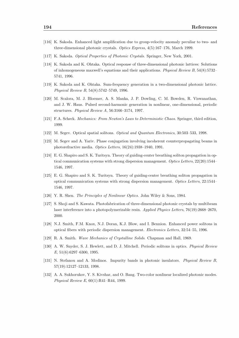
194 References
[116] K. Sakoda. Enhanced light amplification due to group-velocity anomaly peculiar to two- andthree-dimensional photonic crystals. Optics Express, 4(5):167–176, March 1999.
[117] K. Sakoda. Optical Properties of Photonic Crystals. Springer, New York, 2001.
[118] K. Sakoda and K. Ohtaka. Optical response of three-dimensional photonic lattices: Solutionsof inhomogeneous maxwell’s equations and their applications. Physical Review B, 54(8):5732–5741, 1996.
[119] K. Sakoda and K. Ohtaka. Sum-frequency generation in a two-dimensional photonic lattice.Physical Review B, 54(8):5742–5749, 1996.
[120] M. Scalora, M. J. Bloemer, A. S. Manka, J. P. Dowling, C. M. Bowden, R. Viswanathan,and J. W. Haus. Pulsed second-harmonic generation in nonlinear, one-dimensional, periodicstructures. Physical Review A, 56:3166–3174, 1997.
[121] F.A. Scheck. Mechanics: From Newton’s Laws to Deterministic Chaos. Springer, third edition,1999.
[122] M. Segev. Optical spatial solitons. Optical and Quantum Electronics, 30:503–533, 1998.
[123] M. Segev and A. Yariv. Phase conjugation involving incoherent counterpropagating beams inphotorefractive media. Optics Letters, 16(24):1938–1940, 1991.
[124] E. G. Shapiro and S. K. Turitsyn. Theory of guiding-center breathing soliton propagation in op-tical communication systems with strong dispersion management. Optics Letters, 22(20):1544–1546, 1997.
[125] E. G. Shapiro and S. K. Turitsyn. Theory of guiding-center breathing soliton propagation inoptical communication systems with strong dispersion management. Optics Letters, 22:1544–1546, 1997.
[126] Y. R. Shen. The Principles of Nonlinear Optics. John Wiley & Sons, 1984.
[127] S. Shoji and S. Kawata. Photofabrication of three-dimensional photonic crystals by multibeamlaser interference into a photopolymerizable resin. Applied Physics Letters, 76(19):2668–2670,2000.
[128] N.J. Smith, F.M. Knox, N.J. Doran, K.J. Blow, and I. Bennion. Enhanced power solitons inoptical fibers with periodic dispersion management. Electronics Letters, 32:54–55, 1996.
[129] R. A. Smith. Wave Mechanics of Crystalline Solids. Chapman and Hall, 1969.
[130] A. W. Snyder, S. J. Hewlett, and D. J. Mitchell. Periodic solitons in optics. Physical ReviewE, 51(6):6297–6300, 1995.
[131] N. Stefanou and A. Modinos. Impurity bands in photonic insulators. Physical Review B,57(19):12127–12133, 1998.
[132] A. A. Sukhorukov, Y. S. Kivshar, and O. Bang. Two-color nonlinear localized photonic modes.Physical Review E, 60(1):R41–R44, 1999.
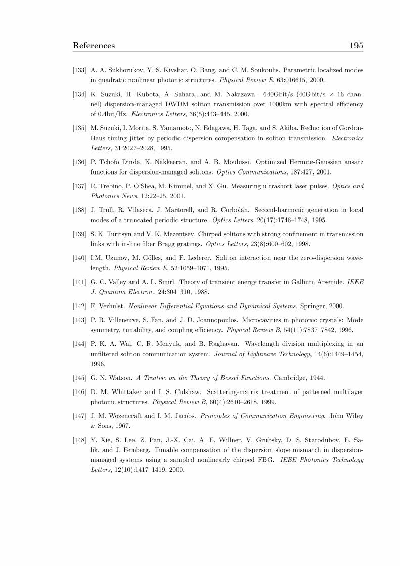
References 195
[133] A. A. Sukhorukov, Y. S. Kivshar, O. Bang, and C. M. Soukoulis. Parametric localized modesin quadratic nonlinear photonic structures. Physical Review E, 63:016615, 2000.
[134] K. Suzuki, H. Kubota, A. Sahara, and M. Nakazawa. 640Gbit/s (40Gbit/s × 16 chan-nel) dispersion-managed DWDM soliton transmission over 1000km with spectral efficiencyof 0.4bit/Hz. Electronics Letters, 36(5):443–445, 2000.
[135] M. Suzuki, I. Morita, S. Yamamoto, N. Edagawa, H. Taga, and S. Akiba. Reduction of Gordon-Haus timing jitter by periodic dispersion compensation in soliton transmission. ElectronicsLetters, 31:2027–2028, 1995.
[136] P. Tchofo Dinda, K. Nakkeeran, and A. B. Moubissi. Optimized Hermite-Gaussian ansatzfunctions for dispersion-managed solitons. Optics Communications, 187:427, 2001.
[137] R. Trebino, P. O’Shea, M. Kimmel, and X. Gu. Measuring ultrashort laser pulses. Optics andPhotonics News, 12:22–25, 2001.
[138] J. Trull, R. Vilaseca, J. Martorell, and R. Corbolan. Second-harmonic generation in localmodes of a truncated periodic structure. Optics Letters, 20(17):1746–1748, 1995.
[139] S. K. Turitsyn and V. K. Mezentsev. Chirped solitons with strong confinement in transmissionlinks with in-line fiber Bragg gratings. Optics Letters, 23(8):600–602, 1998.
[140] I.M. Uzunov, M. Golles, and F. Lederer. Soliton interaction near the zero-dispersion wave-length. Physical Review E, 52:1059–1071, 1995.
[141] G. C. Valley and A. L. Smirl. Theory of transient energy transfer in Gallium Arsenide. IEEEJ. Quantum Electron., 24:304–310, 1988.
[142] F. Verhulst. Nonlinear Differential Equations and Dynamical Systems. Springer, 2000.
[143] P. R. Villeneuve, S. Fan, and J. D. Joannopoulos. Microcavities in photonic crystals: Modesymmetry, tunability, and coupling efficiency. Physical Review B, 54(11):7837–7842, 1996.
[144] P. K. A. Wai, C. R. Menyuk, and B. Raghavan. Wavelength division multiplexing in anunfiltered soliton communication system. Journal of Lightwave Technology, 14(6):1449–1454,1996.
[145] G. N. Watson. A Treatise on the Theory of Bessel Functions. Cambridge, 1944.
[146] D. M. Whittaker and I. S. Culshaw. Scattering-matrix treatment of patterned multilayerphotonic structures. Physical Review B, 60(4):2610–2618, 1999.
[147] J. M. Wozencraft and I. M. Jacobs. Principles of Communication Engineering. John Wiley& Sons, 1967.
[148] Y. Xie, S. Lee, Z. Pan, J.-X. Cai, A. E. Willner, V. Grubsky, D. S. Starodubov, E. Sa-lik, and J. Feinberg. Tunable compensation of the dispersion slope mismatch in dispersion-managed systems using a sampled nonlinearly chirped FBG. IEEE Photonics TechnologyLetters, 12(10):1417–1419, 2000.
196 References
[149] Y. Xu, R.K. Lee, and A. Yariv. Adiabatic coupling between conventional dielectric waveguidesand waveguides with discrete translational symmetry. Optics Letters, 25(10):755–757, 2000.
[150] Y. Xu, R.K. Lee, and A. Yariv. Propagation and second-harmonic generation of electro-magnetic waves in a coupled-resonator optical waveguide. Journal of the Optical Society ofAmerica B, 17(3):387–400, 2000.
[151] T. Yamamoto and M. Nakazawa. Third- and fourth-order active dispersion-compensationwith a phase modulator in a terabit-per-second optical time-division multiplexed transmission.Optics Letters, 26(9):647–649, 2001.
[152] A. Yariv. Quantum Electronics. John Wiley & Sons, third edition, 1989.
[153] A. Yariv. Signal-to-noise considerations in fiber links with periodic or distributed opticalamplification. Optics Letters, 15:1064–1066, 1990.
[154] A. Yariv. Optical Electronics in Modern Communications. Oxford University Press, fifthedition, 1997.
[155] A. Yariv. Steady state repeating optical pulses in a periodic nonlinear fiber. Journal ofNonlinear Optical Physics & Materials, 8(1):165–170, 1999.
[156] A. Yariv, Y. Xu, R. K. Lee, and A. Scherer. Coupled-resonator optical waveguide: a proposaland analysis. Optics Letters, 24(11):711–713, 1999.
[157] A. Yariv and P. Yeh. The application of Gaussian beam formalism to optical propagation innonlinear media. Optics Communications, 27(2):295, 1978.
[158] P. Yeh. Fundamental limit on the speed of photorefractive effect and its impact on deviceapplications and material research. Applied Optics, 26(4):602–604, 1987.
[159] P. Yeh and A. Yariv. Bragg reflection waveguides. Optics Communications, 19:427–430, 1976.
[160] V. E. Zakharov and A. B. Shabat. Exact theory of two-dimensional self-focusing and one-dimensional self-modulation of waves in nonlinear media. Soviet Physics JETP, 34(1):62–69,1972.
[161] J. M. Ziman. Principles of the Theory of Solids. Cambridge University Press, second edition,1998.