Coupled physical–biological modelling study of the East

www.elsevier.com/locate/jmarsys

Journal of Marine System

Coupled physical–biological modelling study of the East Australian

Current with idealised wind forcing: Part II.

Biological dynamical analysis

Mark E. Baird a,*, Patrick G. Timko a, Iain M. Suthers b, Jason H. Middleton a

a Centre for Environmental Modelling and Prediction, School of Mathematics, University of NSW, Sydney NSW, 2052, Australiab School of Biological, Earth and Environmental Sciences, University of NSW, Sydney NSW, 2052, Australia

Received 1 December 2004; accepted 22 September 2005

Available online 19 January 2006

Abstract

A northerly and a southerly wind simulation of a coupled physical–biomechanical NPZ model configured for the East Australian

Current (EAC) are analysed using the relative size of dynamical terms in the biological equations. TheNPZmodel is a configuration of

the Baird et al. [Baird, M.E., Oke, P.R., Suthers, I.M., Middleton, J.H., 2004. A plankton population model with bio-mechanical

descriptions of biological processes in an idealised 2-D ocean basin. J. Mar. Syst. 50, 199–222.] model with biomechanical

descriptions of phytoplankton and zooplankton processes. Analysis of the complete set of dynamical terms affecting the biological

model are presented, including: advection, diffusion, nutrient uptake and light capture, phytoplankton and zooplankton growth,

grazing, and mortality, as well as the local rate of change, or tendency, of the biological state variables. A dynamical analysis is

undertaken at two scales: (1) at the scale of an individual phytoplankton cell of the interaction of light supply, nutrient supply and

organic matter synthesis in determining internal nitrogen and energy reserves, and (2) at the ecosystem scale of phytoplankton and

zooplankton growth in determining dissolved inorganic nitrogen, phytoplankton and zooplankton concentrations. The spatial

distribution of primary and secondary production, an approximation of the f-ratio, and continental shelf fluxes of inorganic and

organic nitrogen are also investigated. As found in Part I of this study, the tracer age provides a useful diagnostic tool for understanding

the affects of the physical forcing on biological processes. The analysis provides a quantification of the biological processes occurring

off the NSW shelf at a spatial scale and interpretive detail which is not possible with the limited in situ sampling of the region.

D 2005 Elsevier B.V. All rights reserved.

Keywords: Phytoplankton; Zooplankton; Processes; Dynamical terms; Primary production; Secondary production

1. Introduction

In natural systems it is often difficult to determine

the relative magnitude of processes that affect the quan-

tity of a particular variable, such as phytoplankton

biomass in the coastal ocean. Typically few, if any,

0924-7963/$ - see front matter D 2005 Elsevier B.V. All rights reserved.

doi:10.1016/j.jmarsys.2005.09.006

* Corresponding author. Tel.: +61 2 9385 7196; fax: +61 2 9385

7123.

E-mail address: [email protected] (M.E. Baird).

measurements are made of the processes that change

the value of an environmental variable. As a result, it is

difficult to determine the dominant processes affecting

an observed time-series. By contrast, with a sufficiently

detailed dynamical analysis of a numerical model, it

should always be possible to quantify why a model

simulation behaves as it does.

The dynamics of complex hydrodynamic and ecolog-

ical models can be quantified by investigating the mag-

nitude of individual terms in the model equations. For

s 59 (2006) 271–291

M.E. Baird et al. / Journal of Marine Systems 59 (2006) 271–291272

example in a hydrodynamic model of shelf circulation

Oke (2002) split the alongshore momentum equation

into tendency, advection, diffusion, ageostrophic, sur-

face stress and bottom stress terms, as a means of quan-

tifying the spatially-resolved relative magnitudes of

these interacting processes. Physical studies have also

included vorticity balances (Mesias and Strub, 2003).

These dynamical balances allow conclusions to be drawn

as to the most quantitatively significant processes driv-

ing observed circulation patterns.

The detailed analysis of terms in marine ecosystem

models is not as common, or as sophisticated, as found

in the physical modelling literature. Nonetheless, the

importance of some biological terms has been well

recognised, and some such as primary productivity

are commonly reported from field experiments and

numerical modelling studies. For example, in two di-

mensional ecosystem models primary productivity, new

production, and secondary productivity have been cal-

culated (Franks and Walstad, 1997; Edwards et al.,

2000).

A coupled physical–biomechanical NPZ model of

the pelagic ecosystem in the East Australian Current

(EAC) off the New South Wales (NSW) coast has been

developed and implemented as described in bCoupledphysical–biological modelling study of the East Aus-

tralian Current with idealised wind forcing. Part I:

Biological model intercomparisonQ (Baird et al., 2006-

this issue). This present paper is an exploration of the

behaviour of the biological quantities in the EAC con-

figuration of the coupled physical–biomechanical NPZ

model, and in particular, an analysis of the spatially

resolved relative magnitude of each of the biological

processes.

The biological model studied in this paper contains

two scales of dynamics. At short timescales within

each phytoplankton cell, a balance exists between the

growth rate of a phytoplankton cell, and the supply of

nitrogen and light energy to the cell. For example, at

an extracellular dissolved inorganic nitrogen (DIN)

concentration of 0.017 mol N m�3 (the maximum in

the model), and a surface light field of 0.05 mol

photon m�2 s-1 (midday summer maximum), the

time for the cell to fill with nitrogen and energy is

approximately 300 and 10 s, respectively. The balance

between nutrient supply, light supply and phytoplank-

ton growth, which largely determines the internal

reserves of nitrogen and energy, is investigated in

Section 3.

Under optimal growing conditions a phytoplankton

cell within the model requires approximately 21,000 s

(or 0.25 d) to use all its nitrogen and energy reserves

and double in biomass, while the model zooplankton

requires 0.5 d to double. The balance of DIN uptake,

phytoplankton growth and zooplankton growth,

which occurs at the population level and over a

timescale of days, is investigated in Section 4. The

dynamical terms which change the DIN concentration,

phytoplankton biomass and zooplankton biomass are

investigated for the same northerly wind (NW) and

southerly wind (SW) simulations used in Baird et al.

(2006-this issue).

Further analysis of the model is undertaken in Sec-

tion 5. Firstly, an analysis of the vertical distribution of

primary productivity (PP) and secondary productivity

(SP) is undertaken. Secondly, the continental shelf flux

of inorganic and organic nitrogen along 900 km of

continental shelf is quantified. And thirdly, the biolog-

ical diagnostic variable f-ratio, the ratio of new produc-

tion to total primary production (Dugdale, 1967; Eppley

and Peterson, 1979), is given and compared to a mea-

sure of the time the water has been above 90 m. These

analyses provide outputs from the model that are com-

monly used in quantifying marine biological processes,

but are difficult to measure over a broad region of the

ocean.

The objective of this study is to provide a detailed

analysis of the Baird et al. (2004) biomechanical model

applied to a northerly wind (NW) and southerly wind

(SW) scenario for the waters off the NSW coast – the

first presentation of a coupled physical-biological

model of the region and the first three dimensional

application of the recently developed biomechanical

model.

2. The coupled physical–biological model

The physical model is the Princeton Ocean Model

(POM) which has a free surface and solves the non-

linear primitive equations on a horizontal orthogonal

curvilinear grid and a vertical sigma (terrain following)

coordinate system using finite difference methods

(Blumberg and Mellor, 1987). The Craig–Banner

scheme (Craig and Banner, 1994) for calculating the

wave-driven flux of turbulent kinetic energy at the

surface has been implemented.

The physical configuration (Fig. 1) extends along

the NSW coast from 28.48 S to 37.58 S, a distance of

1025 km, and extends offshore between 395 km (at

28.48 S) and 500 km (at 37.58 S). The grid has 130

points in the offshore direction with a resolution be-

tween 1 and 6 km, and 82 in the alongshore direction

with a resolution between 6.5 and 24 km. The outer

six boxes on the northern, eastern and southern bound-

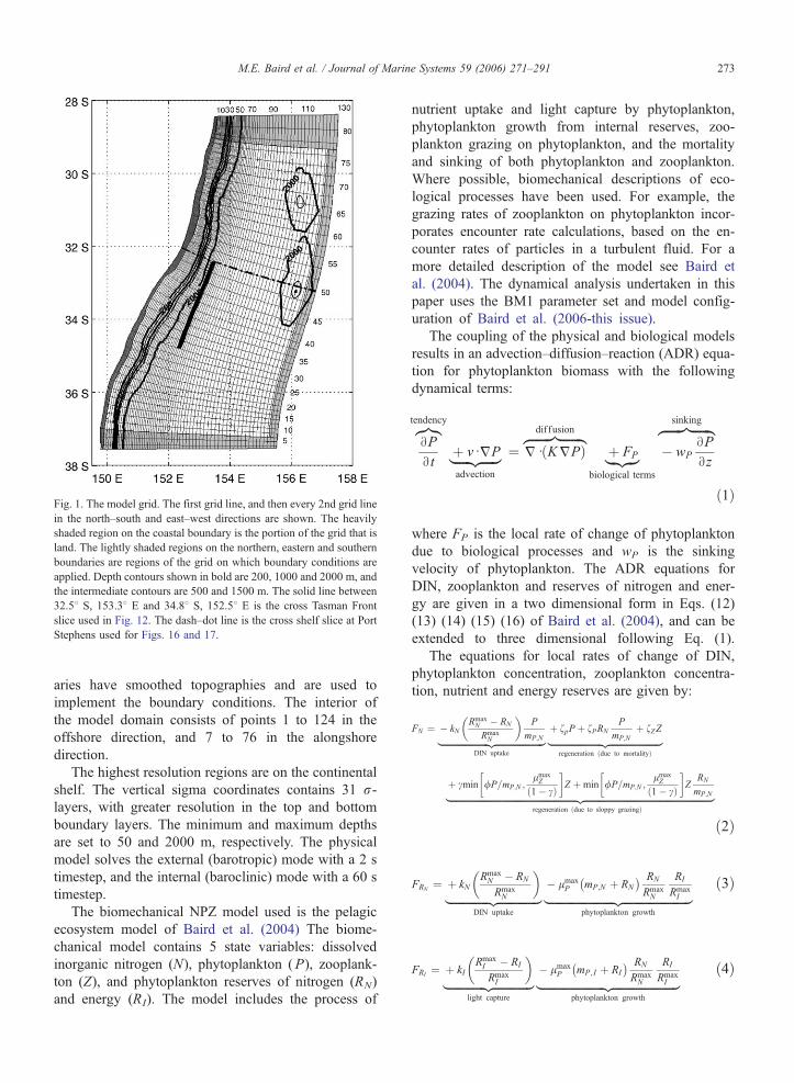
Fig. 1. The model grid. The first grid line, and then every 2nd grid line

in the north–south and east–west directions are shown. The heavily

shaded region on the coastal boundary is the portion of the grid that is

land. The lightly shaded regions on the northern, eastern and southern

boundaries are regions of the grid on which boundary conditions are

applied. Depth contours shown in bold are 200, 1000 and 2000 m, and

the intermediate contours are 500 and 1500 m. The solid line between

32.58 S, 153.38 E and 34.88 S, 152.58 E is the cross Tasman Front

slice used in Fig. 12. The dash–dot line is the cross shelf slice at Port

Stephens used for Figs. 16 and 17.

M.E. Baird et al. / Journal of Marine Systems 59 (2006) 271–291 273

aries have smoothed topographies and are used to

implement the boundary conditions. The interior of

the model domain consists of points 1 to 124 in the

offshore direction, and 7 to 76 in the alongshore

direction.

The highest resolution regions are on the continental

shelf. The vertical sigma coordinates contains 31 r-layers, with greater resolution in the top and bottom

boundary layers. The minimum and maximum depths

are set to 50 and 2000 m, respectively. The physical

model solves the external (barotropic) mode with a 2 s

timestep, and the internal (baroclinic) mode with a 60 s

timestep.

The biomechanical NPZ model used is the pelagic

ecosystem model of Baird et al. (2004) The biome-

chanical model contains 5 state variables: dissolved

inorganic nitrogen (N), phytoplankton (P), zooplank-

ton (Z), and phytoplankton reserves of nitrogen (RN)

and energy (RI). The model includes the process of

nutrient uptake and light capture by phytoplankton,

phytoplankton growth from internal reserves, zoo-

plankton grazing on phytoplankton, and the mortality

and sinking of both phytoplankton and zooplankton.

Where possible, biomechanical descriptions of eco-

logical processes have been used. For example, the

grazing rates of zooplankton on phytoplankton incor-

porates encounter rate calculations, based on the en-

counter rates of particles in a turbulent fluid. For a

more detailed description of the model see Baird et

al. (2004). The dynamical analysis undertaken in this

paper uses the BM1 parameter set and model config-

uration of Baird et al. (2006-this issue).

The coupling of the physical and biological models

results in an advection–diffusion–reaction (ADR) equa-

tion for phytoplankton biomass with the following

dynamical terms:

BP

Bt

z}|{tendency

þ vdjP|fflfflfflfflffl{zfflfflfflfflffl}advection

¼ jd KjPð Þzfflfflfflfflfflfflffl}|fflfflfflfflfflfflffl{dif fusion

þ FP|fflffl{zfflffl}biological terms

� wP

BP

Bz

zfflfflfflfflfflffl}|fflfflfflfflfflffl{sinking

ð1Þ

where FP is the local rate of change of phytoplankton

due to biological processes and wP is the sinking

velocity of phytoplankton. The ADR equations for

DIN, zooplankton and reserves of nitrogen and ener-

gy are given in a two dimensional form in Eqs. (12)

(13) (14) (15) (16) of Baird et al. (2004), and can be

extended to three dimensional following Eq. (1).

The equations for local rates of change of DIN,

phytoplankton concentration, zooplankton concentra-

tion, nutrient and energy reserves are given by:

FN ¼ � kNRmaxN � RN

RmaxN

� �P

mP;N|fflfflfflfflfflfflfflfflfflfflfflfflfflfflfflfflfflfflfflfflfflffl{zfflfflfflfflfflfflfflfflfflfflfflfflfflfflfflfflfflfflfflfflfflffl}DIN uptake

þ fpP þ fPRN

P

mP;Nþ fZZ|fflfflfflfflfflfflfflfflfflfflfflfflfflfflfflfflfflfflfflfflfflfflffl{zfflfflfflfflfflfflfflfflfflfflfflfflfflfflfflfflfflfflfflfflfflfflffl}

regeneration due to mortalityð Þ

þ cmin /P=mP;N ;lmaxZ

1� cð Þ

� �Z þmin /P=mP;N ;

lmaxZ

1� cð Þ

� �Z

RN

mP;N|fflfflfflfflfflfflfflfflfflfflfflfflfflfflfflfflfflfflfflfflfflfflfflfflfflfflfflfflfflfflfflfflfflfflfflfflfflfflfflfflfflfflfflfflfflfflfflfflfflfflfflfflfflfflfflfflfflfflffl{zfflfflfflfflfflfflfflfflfflfflfflfflfflfflfflfflfflfflfflfflfflfflfflfflfflfflfflfflfflfflfflfflfflfflfflfflfflfflfflfflfflfflfflfflfflfflfflfflfflfflfflfflfflfflfflfflfflfflffl}regeneration ðdue to sloppy grazingÞ

ð2Þ

FRN¼ þ kN

RmaxN � RN

RmaxN

� �|fflfflfflfflfflfflfflfflfflfflfflfflfflfflfflffl{zfflfflfflfflfflfflfflfflfflfflfflfflfflfflfflffl}

DIN uptake

� lmaxP mP;N þ RN

� � RN

RmaxN

RI

RmaxI|fflfflfflfflfflfflfflfflfflfflfflfflfflfflfflfflfflfflfflfflfflfflfflfflfflfflffl{zfflfflfflfflfflfflfflfflfflfflfflfflfflfflfflfflfflfflfflfflfflfflfflfflfflfflffl}

phytoplankton growth

ð3Þ

FRI¼ þ kI

RmaxI � RI

RmaxI

� �|fflfflfflfflfflfflfflfflfflfflfflfflfflfflffl{zfflfflfflfflfflfflfflfflfflfflfflfflfflfflffl}

light capture

� lmaxP mP; I þ RI

� � RN

RmaxN

RI

RmaxI|fflfflfflfflfflfflfflfflfflfflfflfflfflfflfflfflfflfflfflfflfflfflfflfflfflffl{zfflfflfflfflfflfflfflfflfflfflfflfflfflfflfflfflfflfflfflfflfflfflfflfflfflffl}

phytoplankton growth

ð4Þ


FP ¼ þ lmaxP

RN

RmaxN

RI

RmaxI

P

|fflfflfflfflfflfflfflfflfflfflfflfflfflfflfflffl{zfflfflfflfflfflfflfflfflfflfflfflfflfflfflfflffl}phytoplankton growth

�min /P=mP;N ;lmaxZ

1� cð Þ

� �Z

|fflfflfflfflfflfflfflfflfflfflfflfflfflfflfflfflfflfflfflfflfflfflfflfflffl{zfflfflfflfflfflfflfflfflfflfflfflfflfflfflfflfflfflfflfflfflfflfflfflfflffl}grazing

� fPP|fflfflffl{zfflfflffl}mortality

ð5ÞFZ ¼ þmin /P=mP;N ;

lmaxZ

1� cð Þ

� �Z � cmin /P=mP;N ;

lmaxZ

1� cð Þ

� �Z

|fflfflfflfflfflfflfflfflfflfflfflfflfflfflfflfflfflfflfflfflfflfflfflfflfflfflfflfflfflfflfflfflfflfflfflfflfflfflfflfflfflfflfflfflfflfflfflfflfflfflfflfflfflffl{zfflfflfflfflfflfflfflfflfflfflfflfflfflfflfflfflfflfflfflfflfflfflfflfflfflfflfflfflfflfflfflfflfflfflfflfflfflfflfflfflfflfflfflfflfflfflfflfflfflfflfflfflfflffl}zooplankton growth

� fZZ|fflfflffl{zfflfflffl}mortality

ð6Þwhere kN and kI are the maximum rates of DIN and

energy uptake of phytoplankton, respectively (and are a

function of N and incident light, respectively), RNmax

and RImax are the maximum values of RN and RI,

respectively; lPmax and lZ

max are the maximum growth

rates of phytoplankton and zooplankton, respectively, /is the encounter rate coefficient between phytoplankton

and zooplankton, fP and fZ are the mortality rates of

phytoplankton and zooplankton, respectively, and

(1�c) is the assimilation efficiency of grazing. The

local time derivatives FN, FP and FZ have units of mol

N m�3 s�1, while FRNhas units of mol N cell�1 s�1,

and FRIhas units of mol photon cell�1 s�1. The term P/

mP,N which appears in the DIN uptake and the phyto-

plankton grazing terms, is the concentration of phyto-

plankton cells. Further explanation of these equations is

given in Baird et al. (2004).

2.1. Description of the terms

The dynamical terms of N, P and Z are reported as

either rates of change of the concentration [mol N m�3

s�1], or as a depth-integrated rate of change [mol N

m�2 s�1, mg C m�2 d�1]. The dynamical terms for

internal reserves are determined per cell, and have units

of mol N cell�1 s�1 or mol photon cell�1 s�1. Some

processes, such as DIN uptake, result in a change in

both a concentration of a water column property, and in

the reserves per cell. To convert the rates between the

two scales, the rate of the water column property must

be divided by the concentration of cells, P/mN, as

illustrated for DIN uptake in Eqs. (2) and (3).

The terms analysed are: advection and diffusion of

all biological tracers; DIN uptake; regeneration of DIN

from phytoplankton and zooplankton mortality, and

from sloppy grazing; phytoplankton growth; phyto-

plankton mortality due to zooplankton grazing; zoo-

plankton growth; and zooplankton mortality. Each of

the biological terms is distinguished by curly brackets

in Eqs. (2)–(6).

Tendency terms. For all biological state variables,

the tendency term is the local rate of change of the

variable with respect to time. Tendency will be the sum

of all physical and biological terms.

Physical terms. The advection term accounts for the

transport of a scalar (i.e., the biological state variables)

from one location to another due to water motion that is

resolved by the hydrodynamic model. At a particular

location, the advection term represents the balance

between the flux of a scalar into the volume due to

resolved water motion, and the flux out. The diffusion

term (turbulent mixing) accounts for the transport of a

scalar from a region of high concentration to a region of

low concentration as a result of water motion that is

below the resolution of the physical model. In this

paper only vertical diffusion is reported. Horizontal

diffusion is included in the calculation of the advection

term by the physical model, and is incorporated in the

advection term in the following analysis.

Biological terms. The DIN uptake term accounts for

the rate of change in concentration of DIN in the water

column due to uptake into phytoplankton internal

reserves (RN). The DIN uptake term is always negative

for N and positive for RN. The regeneration term is the

rate of change in N due to the processes of zooplankton

and phytoplankton mortality and the inefficient (or

sloppy) grazing of phytoplankton, and is always posi-

tive. Note that during grazing the nitrogen held as

internal reserves (RN) of grazed phytoplankton forms

a part of the sloppy grazing component of the regener-

ation term. The other component is the inefficient use

of the organic matter in zooplankton growth.

The phytoplankton growth term, or primary produc-

tivity, is the rate of change in concentration of phyto-

plankton due to the combination of internal reserves of

nitrogen, RN, and energy, RI, to create organic matter

(at a photon :N ratio of 1060 :16). Phytoplankton

growth is always positive for P and negative for RN

and RI. The grazing term is the rate of change in

concentration of phytoplankton due to the grazing by

zooplankton, and is always negative. The phytoplank-

ton mortality term is the rate of change in concentration

of phytoplankton (always negative) due to death of

cells through processes other than zooplankton grazing.

The zooplankton growth term, or secondary produc-

tion, is the rate of change in concentration of zooplank-

ton due to grazing on phytoplankton and is always

positive. Note that zooplankton growth is based on

zooplankton consuming only the nitrogen held as organ-

ic matter in the phytoplankton, and not that held as

internal reserves. Zooplankton growth is approximately

30% of the loss rate of phytoplankton due to grazing, a

result of the inefficiency of ingestion processes. The

zooplankton mortality term is the rate of change in

concentration of zooplankton (always negative) due to

loss of zooplankton nitrogen through all biological pro-


cesses, and represents such processes as excretion, def-

ecation, viral death, and higher order mortality terms.

2.2. Simulation details

The upwelling favourable northerly wind (NW) and

downwelling favourable southerly wind (SW) simula-

tions are those which have already been described in

Part I: Biological model intercomparison (Baird et al.,

2006-this issue) and are implemented on the computa-

tional grid shown in Fig. 1. The NW and SW simula-

tions are forced with a 0.1 N m�2 surface stress which

corresponds to a wind of approximately 5 m s�1. The

terms for the DIN, phytoplankton and zooplankton

fields are the averaged over an inertial period (=|2p/C|=0.9022 d, where �8.06�10�5 s�1 is the Coriolis

parameter in the centre of the model domain). The

terms for RN and RI are not time averaged, as the

timescale for the dynamics of RN and RI is much less

than the inertial period, and close to the model timestep.

3. Dynamical analysis of RN and RI

Within each phytoplankton cell, a dynamical balance

exists between the processes of nutrient uptake, light

capture and phytoplankton growth which determines

the value of the nitrogen reserves (Eq. (3)) and energy

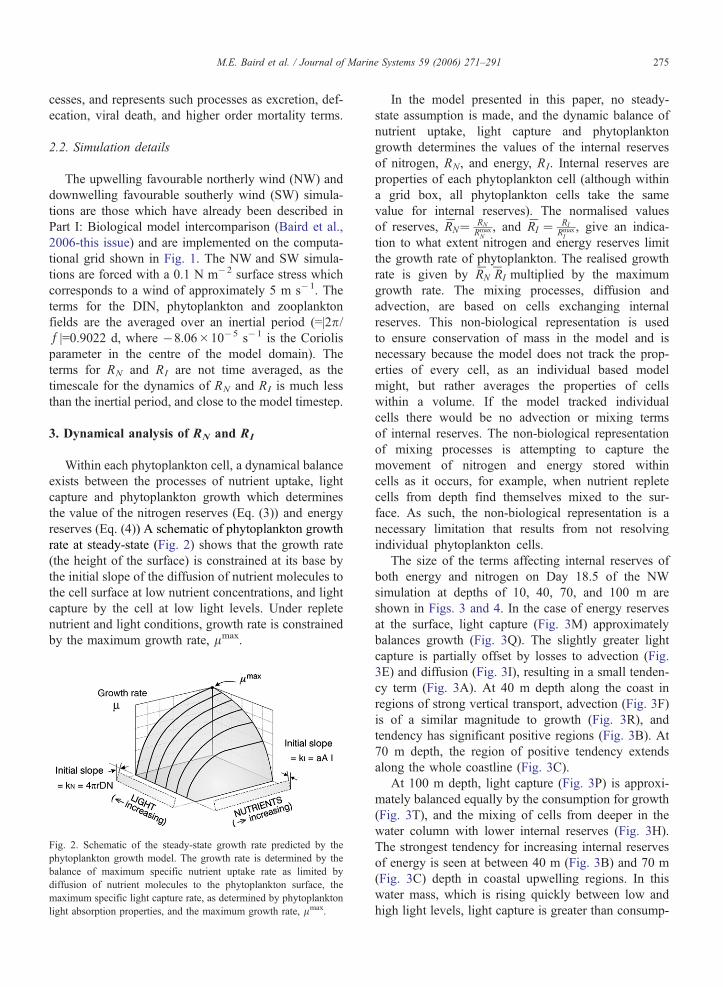
reserves (Eq. (4)) A schematic of phytoplankton growth

rate at steady-state (Fig. 2) shows that the growth rate

(the height of the surface) is constrained at its base by

the initial slope of the diffusion of nutrient molecules to

the cell surface at low nutrient concentrations, and light

capture by the cell at low light levels. Under replete

nutrient and light conditions, growth rate is constrained

by the maximum growth rate, lmax.

Fig. 2. Schematic of the steady-state growth rate predicted by the

phytoplankton growth model. The growth rate is determined by the

balance of maximum specific nutrient uptake rate as limited by

diffusion of nutrient molecules to the phytoplankton surface, the

maximum specific light capture rate, as determined by phytoplankton

light absorption properties, and the maximum growth rate, lmax.

In the model presented in this paper, no steady-

state assumption is made, and the dynamic balance of

nutrient uptake, light capture and phytoplankton

growth determines the values of the internal reserves

of nitrogen, RN, and energy, RI. Internal reserves are

properties of each phytoplankton cell (although within

a grid box, all phytoplankton cells take the same

value for internal reserves). The normalised values

of reserves, RN

P ¼ RN

RmaxN

, and RI

P ¼ RI

RmaxI

, give an indica-

tion to what extent nitrogen and energy reserves limit

the growth rate of phytoplankton. The realised growth

rate is given by RN

PRI

Pmultiplied by the maximum

growth rate. The mixing processes, diffusion and

advection, are based on cells exchanging internal

reserves. This non-biological representation is used

to ensure conservation of mass in the model and is

necessary because the model does not track the prop-

erties of every cell, as an individual based model

might, but rather averages the properties of cells

within a volume. If the model tracked individual

cells there would be no advection or mixing terms

of internal reserves. The non-biological representation

of mixing processes is attempting to capture the

movement of nitrogen and energy stored within

cells as it occurs, for example, when nutrient replete

cells from depth find themselves mixed to the sur-

face. As such, the non-biological representation is a

necessary limitation that results from not resolving

individual phytoplankton cells.

The size of the terms affecting internal reserves of

both energy and nitrogen on Day 18.5 of the NW

simulation at depths of 10, 40, 70, and 100 m are

shown in Figs. 3 and 4. In the case of energy reserves

at the surface, light capture (Fig. 3M) approximately

balances growth (Fig. 3Q). The slightly greater light

capture is partially offset by losses to advection (Fig.

3E) and diffusion (Fig. 3I), resulting in a small tenden-

cy term (Fig. 3A). At 40 m depth along the coast in

regions of strong vertical transport, advection (Fig. 3F)

is of a similar magnitude to growth (Fig. 3R), and

tendency has significant positive regions (Fig. 3B). At

70 m depth, the region of positive tendency extends

along the whole coastline (Fig. 3C).

At 100 m depth, light capture (Fig. 3P) is approxi-

mately balanced equally by the consumption for growth

(Fig. 3T), and the mixing of cells from deeper in the

water column with lower internal reserves (Fig. 3H).

The strongest tendency for increasing internal reserves

of energy is seen at between 40 m (Fig. 3B) and 70 m

(Fig. 3C) depth in coastal upwelling regions. In this

water mass, which is rising quickly between low and

high light levels, light capture is greater than consump-

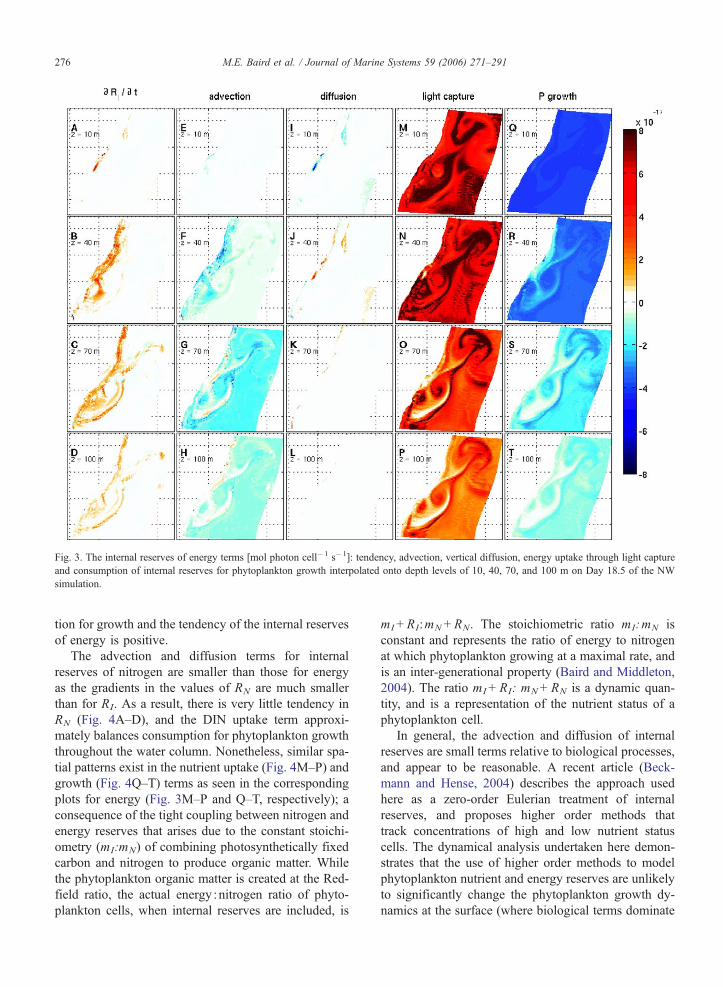
Fig. 3. The internal reserves of energy terms [mol photon cell�1 s�1]: tendency, advection, vertical diffusion, energy uptake through light capture

and consumption of internal reserves for phytoplankton growth interpolated onto depth levels of 10, 40, 70, and 100 m on Day 18.5 of the NW

simulation.


tion for growth and the tendency of the internal reserves

of energy is positive.

The advection and diffusion terms for internal

reserves of nitrogen are smaller than those for energy

as the gradients in the values of RN are much smaller

than for RI. As a result, there is very little tendency in

RN (Fig. 4A–D), and the DIN uptake term approxi-

mately balances consumption for phytoplankton growth

throughout the water column. Nonetheless, similar spa-

tial patterns exist in the nutrient uptake (Fig. 4M–P) and

growth (Fig. 4Q–T) terms as seen in the corresponding

plots for energy (Fig. 3M–P and Q–T, respectively); a

consequence of the tight coupling between nitrogen and

energy reserves that arises due to the constant stoichi-

ometry (mI:mN) of combining photosynthetically fixed

carbon and nitrogen to produce organic matter. While

the phytoplankton organic matter is created at the Red-

field ratio, the actual energy :nitrogen ratio of phyto-

plankton cells, when internal reserves are included, is

mI +RI:mN+RN. The stoichiometric ratio mI:mN is

constant and represents the ratio of energy to nitrogen

at which phytoplankton growing at a maximal rate, and

is an inter-generational property (Baird and Middleton,

2004). The ratio mI+RI: mN+RN is a dynamic quan-

tity, and is a representation of the nutrient status of a

phytoplankton cell.

In general, the advection and diffusion of internal

reserves are small terms relative to biological processes,

and appear to be reasonable. A recent article (Beck-

mann and Hense, 2004) describes the approach used

here as a zero-order Eulerian treatment of internal

reserves, and proposes higher order methods that

track concentrations of high and low nutrient status

cells. The dynamical analysis undertaken here demon-

strates that the use of higher order methods to model

phytoplankton nutrient and energy reserves are unlikely

to significantly change the phytoplankton growth dy-

namics at the surface (where biological terms dominate

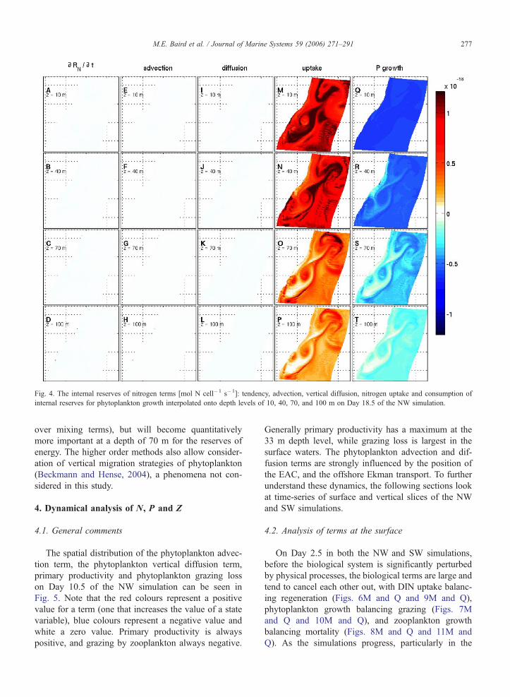
Fig. 4. The internal reserves of nitrogen terms [mol N cell�1 s�1]: tendency, advection, vertical diffusion, nitrogen uptake and consumption of

internal reserves for phytoplankton growth interpolated onto depth levels of 10, 40, 70, and 100 m on Day 18.5 of the NW simulation.


over mixing terms), but will become quantitatively

more important at a depth of 70 m for the reserves of

energy. The higher order methods also allow consider-

ation of vertical migration strategies of phytoplankton

(Beckmann and Hense, 2004), a phenomena not con-

sidered in this study.

4. Dynamical analysis of N, P and Z

4.1. General comments

The spatial distribution of the phytoplankton advec-

tion term, the phytoplankton vertical diffusion term,

primary productivity and phytoplankton grazing loss

on Day 10.5 of the NW simulation can be seen in

Fig. 5. Note that the red colours represent a positive

value for a term (one that increases the value of a state

variable), blue colours represent a negative value and

white a zero value. Primary productivity is always

positive, and grazing by zooplankton always negative.

Generally primary productivity has a maximum at the

33 m depth level, while grazing loss is largest in the

surface waters. The phytoplankton advection and dif-

fusion terms are strongly influenced by the position of

the EAC, and the offshore Ekman transport. To further

understand these dynamics, the following sections look

at time-series of surface and vertical slices of the NW

and SW simulations.

4.2. Analysis of terms at the surface

On Day 2.5 in both the NW and SW simulations,

before the biological system is significantly perturbed

by physical processes, the biological terms are large and

tend to cancel each other out, with DIN uptake balanc-

ing regeneration (Figs. 6M and Q and 9M and Q),

phytoplankton growth balancing grazing (Figs. 7M

and Q and 10M and Q), and zooplankton growth

balancing mortality (Figs. 8M and Q and 11M and

Q). As the simulations progress, particularly in the

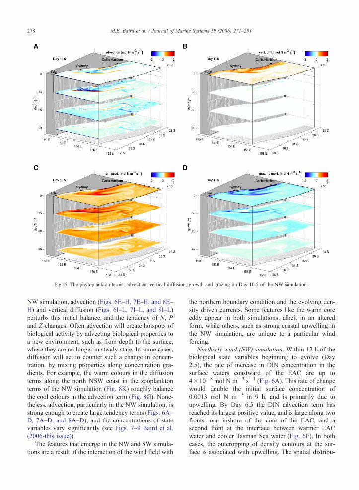
Fig. 5. The phytoplankton terms: advection, vertical diffusion, growth and grazing on Day 10.5 of the NW simulation.


NW simulation, advection (Figs. 6E–H, 7E–H, and 8E–

H) and vertical diffusion (Figs. 6I–L, 7I–L, and 8I–L)

perturbs this initial balance, and the tendency of N, P

and Z changes. Often advection will create hotspots of

biological activity by advecting biological properties to

a new environment, such as from depth to the surface,

where they are no longer in steady-state. In some cases,

diffusion will act to counter such a change in concen-

tration, by mixing properties along concentration gra-

dients. For example, the warm colours in the diffusion

terms along the north NSW coast in the zooplankton

terms of the NW simulation (Fig. 8K) roughly balance

the cool colours in the advection term (Fig. 8G). None-

theless, advection, particularly in the NW simulation, is

strong enough to create large tendency terms (Figs. 6A–

D, 7A–D, and 8A–D), and the concentrations of state

variables vary significantly (see Figs. 7–9 Baird et al.

(2006-this issue)).

The features that emerge in the NW and SW simula-

tions are a result of the interaction of the wind field with

the northern boundary condition and the evolving den-

sity driven currents. Some features like the warm core

eddy appear in both simulations, albeit in an altered

form, while others, such as strong coastal upwelling in

the NW simulation, are unique to a particular wind

forcing.

Northerly wind (NW) simulation. Within 12 h of the

biological state variables beginning to evolve (Day

2.5), the rate of increase in DIN concentration in the

surface waters coastward of the EAC are up to

4�10�8 mol N m�3 s�1 (Fig. 6A). This rate of change

would double the initial surface concentration of

0.0013 mol N m�3 in 9 h, and is primarily due to

upwelling. By Day 6.5 the DIN advection term has

reached its largest positive value, and is large along two

fronts: one inshore of the core of the EAC, and a

second front at the interface between warmer EAC

water and cooler Tasman Sea water (Fig. 6F). In both

cases, the outcropping of density contours at the sur-

face is associated with upwelling. The spatial distribu-

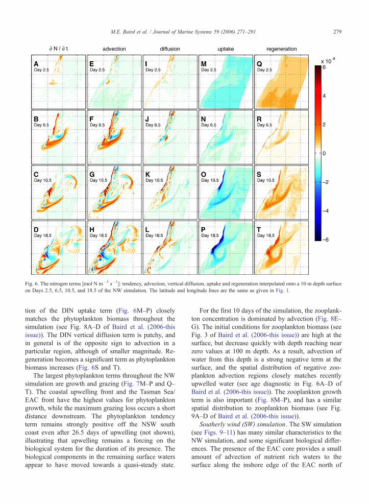
Fig. 6. The nitrogen terms [mol N m�3 s�1]: tendency, advection, vertical diffusion, uptake and regeneration interpolated onto a 10 m depth surface

on Days 2.5, 6.5, 10.5, and 18.5 of the NW simulation. The latitude and longitude lines are the same as given in Fig. 1.


tion of the DIN uptake term (Fig. 6M–P) closely

matches the phytoplankton biomass throughout the

simulation (see Fig. 8A–D of Baird et al. (2006-this

issue)). The DIN vertical diffusion term is patchy, and

in general is of the opposite sign to advection in a

particular region, although of smaller magnitude. Re-

generation becomes a significant term as phytoplankton

biomass increases (Fig. 6S and T).

The largest phytoplankton terms throughout the NW

simulation are growth and grazing (Fig. 7M–P and Q–

T). The coastal upwelling front and the Tasman Sea/

EAC front have the highest values for phytoplankton

growth, while the maximum grazing loss occurs a short

distance downstream. The phytoplankton tendency

term remains strongly positive off the NSW south

coast even after 26.5 days of upwelling (not shown),

illustrating that upwelling remains a forcing on the

biological system for the duration of its presence. The

biological components in the remaining surface waters

appear to have moved towards a quasi-steady state.

For the first 10 days of the simulation, the zooplank-

ton concentration is dominated by advection (Fig. 8E–

G). The initial conditions for zooplankton biomass (see

Fig. 3 of Baird et al. (2006-this issue)) are high at the

surface, but decrease quickly with depth reaching near

zero values at 100 m depth. As a result, advection of

water from this depth is a strong negative term at the

surface, and the spatial distribution of negative zoo-

plankton advection regions closely matches recently

upwelled water (see age diagnostic in Fig. 6A–D of

Baird et al. (2006-this issue)). The zooplankton growth

term is also important (Fig. 8M–P), and has a similar

spatial distribution to zooplankton biomass (see Fig.

9A–D of Baird et al. (2006-this issue)).

Southerly wind (SW) simulation. The SW simulation

(see Figs. 9–11) has many similar characteristics to the

NW simulation, and some significant biological differ-

ences. The presence of the EAC core provides a small

amount of advection of nutrient rich waters to the

surface along the inshore edge of the EAC north of

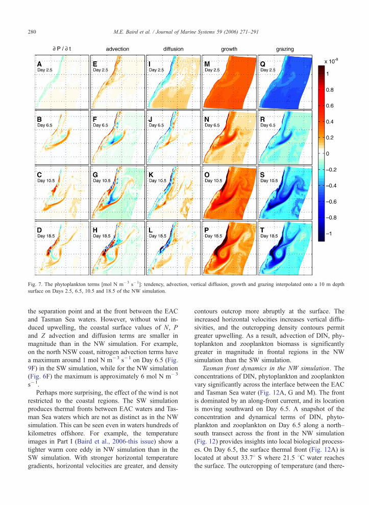
Fig. 7. The phytoplankton terms [mol N m�3 s�1]: tendency, advection, vertical diffusion, growth and grazing interpolated onto a 10 m depth

surface on Days 2.5, 6.5, 10.5 and 18.5 of the NW simulation.


the separation point and at the front between the EAC

and Tasman Sea waters. However, without wind in-

duced upwelling, the coastal surface values of N, P

and Z advection and diffusion terms are smaller in

magnitude than in the NW simulation. For example,

on the north NSW coast, nitrogen advection terms have

a maximum around 1 mol N m�3 s�1 on Day 6.5 (Fig.

9F) in the SW simulation, while for the NW simulation

(Fig. 6F) the maximum is approximately 6 mol N m�3

s�1.

Perhaps more surprising, the effect of the wind is not

restricted to the coastal regions. The SW simulation

produces thermal fronts between EAC waters and Tas-

man Sea waters which are not as distinct as in the NW

simulation. This can be seen even in waters hundreds of

kilometres offshore. For example, the temperature

images in Part I (Baird et al., 2006-this issue) show a

tighter warm core eddy in NW simulation than in the

SW simulation. With stronger horizontal temperature

gradients, horizontal velocities are greater, and density

contours outcrop more abruptly at the surface. The

increased horizontal velocities increases vertical diffu-

sivities, and the outcropping density contours permit

greater upwelling. As a result, advection of DIN, phy-

toplankton and zooplankton biomass is significantly

greater in magnitude in frontal regions in the NW

simulation than the SW simulation.

Tasman front dynamics in the NW simulation. The

concentrations of DIN, phytoplankton and zooplankton

vary significantly across the interface between the EAC

and Tasman Sea water (Fig. 12A, G and M). The front

is dominated by an along-front current, and its location

is moving southward on Day 6.5. A snapshot of the

concentration and dynamical terms of DIN, phyto-

plankton and zooplankton on Day 6.5 along a north–

south transect across the front in the NW simulation

(Fig. 12) provides insights into local biological process-

es. On Day 6.5, the surface thermal front (Fig. 12A) is

located at about 33.78 S where 21.5 8C water reaches

the surface. The outcropping of temperature (and there-

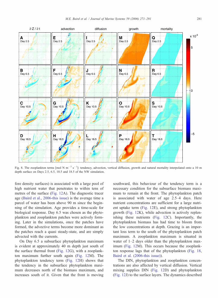
Fig. 8. The zooplankton terms [mol N m�3 s�1]: tendency, advection, vertical diffusion, growth and natural mortality interpolated onto a 10 m

depth surface on Days 2.5, 6.5, 10.5 and 18.5 of the NW simulation.


fore density surfaces) is associated with a large pool of

high nutrient water that penetrates to within tens of

metres of the surface (Fig. 12A). The diagnostic tracer

age (Baird et al., 2006-this issue) is the average time a

parcel of water has been above 90 m since the begin-

ning of the simulation. Age provides a time-scale for

biological response. Day 6.5 was chosen as the phyto-

plankton and zooplankton patches were actively form-

ing. Later in the simulations, once the patches have

formed, the advective terms become more dominant as

the patches reach a quasi steady-state, and are simply

advected with the currents.

On Day 6.5 a subsurface phytoplankton maximum

is evident at approximately 40 m depth just south of

the surface thermal front (Fig. 12G), with a zooplank-

ton maximum further south again (Fig. 12M). The

phytoplankton tendency term (Fig. 12H) shows that

the tendency in the subsurface phytoplankton maxi-

mum decreases north of the biomass maximum, and

increases south of it. Given that the front is moving

southward, this behaviour of the tendency term is a

necessary condition for the subsurface biomass maxi-

mum to remain at the front. The phytoplankton patch

is associated with water of age 2.5–4 days. Here

nutrient concentrations are sufficient for a large nutri-

ent uptake term (Fig. 12E), and strong phytoplankton

growth (Fig. 12K), while advection is actively replen-

ishing these nutrients (Fig. 12C). Importantly, the

phytoplankton biomass has had time to bloom from

the low concentrations at depth. Grazing is an impor-

tant loss term to the south of the phytoplankton patch

maximum. A zooplankton maximum is situated in

water of 1–2 days older than the phytoplankton max-

imum (Fig. 12M). This occurs because the zooplank-

ton response lags that of the phytoplankton (Fig. 18,

Baird et al. (2006-this issue)).

The DIN, phytoplankton and zooplankton concen-

trations are also affected by vertical diffusion. Vertical

mixing supplies DIN (Fig. 12D) and phytoplankton

(Fig. 12J) to the surface layers. The dynamics described

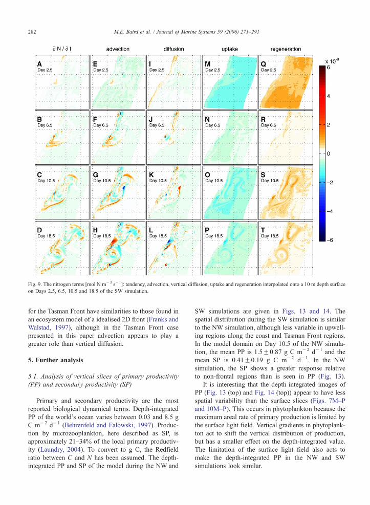
Fig. 9. The nitrogen terms [mol N m�3 s�1]: tendency, advection, vertical diffusion, uptake and regeneration interpolated onto a 10 m depth surface

on Days 2.5, 6.5, 10.5 and 18.5 of the SW simulation.


for the Tasman Front have similarities to those found in

an ecosystem model of a idealised 2D front (Franks and

Walstad, 1997), although in the Tasman Front case

presented in this paper advection appears to play a

greater role than vertical diffusion.

5. Further analysis

5.1. Analysis of vertical slices of primary productivity

(PP) and secondary productivity (SP)

Primary and secondary productivity are the most

reported biological dynamical terms. Depth-integrated

PP of the world’s ocean varies between 0.03 and 8.5 g

C m�2 d�1 (Behrenfeld and Falowski, 1997). Produc-

tion by microzooplankton, here described as SP, is

approximately 21–34% of the local primary productiv-

ity (Laundry, 2004). To convert to g C, the Redfield

ratio between C and N has been assumed. The depth-

integrated PP and SP of the model during the NW and

SW simulations are given in Figs. 13 and 14. The

spatial distribution during the SW simulation is similar

to the NW simulation, although less variable in upwell-

ing regions along the coast and Tasman Front regions.

In the model domain on Day 10.5 of the NW simula-

tion, the mean PP is 1.5F0.87 g C m�2 d�1 and the

mean SP is 0.41F0.19 g C m�2 d�1. In the NW

simulation, the SP shows a greater response relative

to non-frontal regions than is seen in PP (Fig. 13).

It is interesting that the depth-integrated images of

PP (Fig. 13 (top) and Fig. 14 (top)) appear to have less

spatial variability than the surface slices (Figs. 7M–P

and 10M–P). This occurs in phytoplankton because the

maximum areal rate of primary production is limited by

the surface light field. Vertical gradients in phytoplank-

ton act to shift the vertical distribution of production,

but has a smaller effect on the depth-integrated value.

The limitation of the surface light field also acts to

make the depth-integrated PP in the NW and SW

simulations look similar.

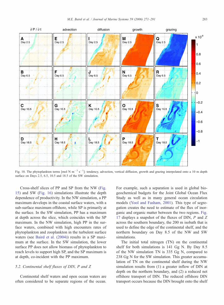
Fig. 10. The phytoplankton terms [mol N m�3 s�1]: tendency, advection, vertical diffusion, growth and grazing interpolated onto a 10 m depth

surface on Days 2.5, 6.5, 10.5 and 18.5 of the SW simulation.


Cross-shelf slices of PP and SP from the NW (Fig.

15) and SW (Fig. 16) simulations illustrate the depth

dependence of productivity. In the NW simulation, a PP

maximum develops in the coastal surface waters, with a

sub-surface maximum offshore, while SP is primarily at

the surface. In the SW simulation, PP has a maximum

at depth across the slice, which coincides with the SP

maximum. In the NW simulation, high PP in the sur-

face waters, combined with high encounters rates of

phytoplankton and zooplankton in the turbulent surface

waters (see Baird et al. (2004)) results in a SP maxi-

mum at the surface. In the SW simulation, the lower

surface PP does not allow biomass of phytoplankton to

reach levels to support high SP, and the SP maximum is

at depth, co-incident with the PP maximum.

5.2. Continental shelf fluxes of DIN, P and Z

Continental shelf waters and open ocean waters are

often considered to be separate regions of the ocean.

For example, such a separation is used in global bio-

geochemical budgets for the Joint Global Ocean Flux

Study as well as in many general ocean circulation

models (Yool and Fasham, 2001). This type of segre-

gation creates the need to estimate of the flux of inor-

ganic and organic matter between the two regions. Fig.

17 displays a snapshot of the fluxes of DIN, P and Z

across the southern boundary, the 200 m isobath that is

used to define the edge of the continental shelf, and the

northern boundary on Day 8.5 of the NW and SW

simulations.

The initial total nitrogen (TN) on the continental

shelf for both simulations is 141 Gg N. By Day 8.5

of the NW simulation TN is 335 Gg N, compared to

238 Gg N for the SW simulation. This greater accumu-

lation of TN on the continental shelf during the NW

simulation results from (1) a greater inflow of DIN at

depth on the northern boundary, and (2) a reduced net

offshore transport of DIN. The reduced offshore DIN

transport occurs because the DIN brought onto the shelf

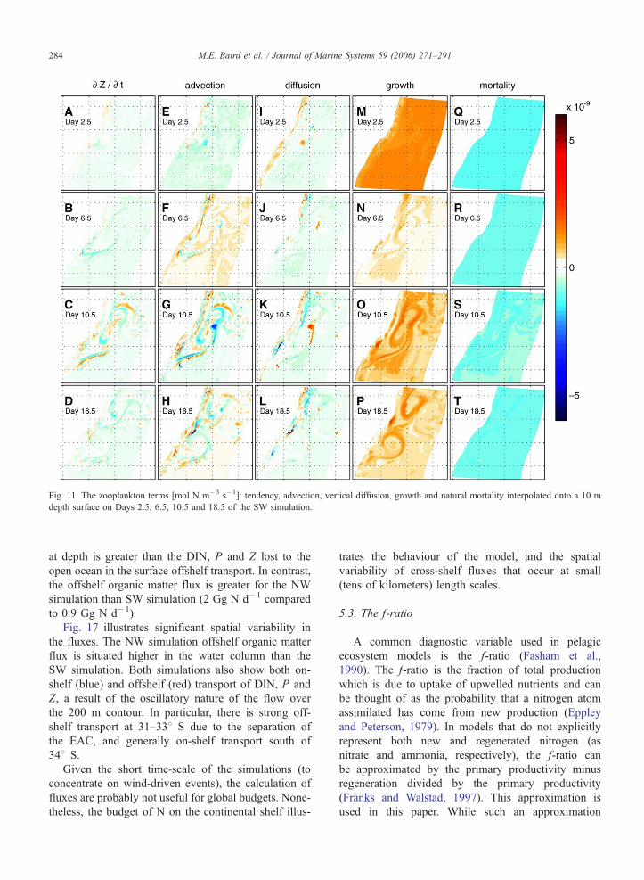
Fig. 11. The zooplankton terms [mol N m�3 s�1]: tendency, advection, vertical diffusion, growth and natural mortality interpolated onto a 10 m

depth surface on Days 2.5, 6.5, 10.5 and 18.5 of the SW simulation.


at depth is greater than the DIN, P and Z lost to the

open ocean in the surface offshelf transport. In contrast,

the offshelf organic matter flux is greater for the NW

simulation than SW simulation (2 Gg N d�1 compared

to 0.9 Gg N d�1).

Fig. 17 illustrates significant spatial variability in

the fluxes. The NW simulation offshelf organic matter

flux is situated higher in the water column than the

SW simulation. Both simulations also show both on-

shelf (blue) and offshelf (red) transport of DIN, P and

Z, a result of the oscillatory nature of the flow over

the 200 m contour. In particular, there is strong off-

shelf transport at 31–338 S due to the separation of

the EAC, and generally on-shelf transport south of

348 S.

Given the short time-scale of the simulations (to

concentrate on wind-driven events), the calculation of

fluxes are probably not useful for global budgets. None-

theless, the budget of N on the continental shelf illus-

trates the behaviour of the model, and the spatial

variability of cross-shelf fluxes that occur at small

(tens of kilometers) length scales.

5.3. The f-ratio

A common diagnostic variable used in pelagic

ecosystem models is the f-ratio (Fasham et al.,

1990). The f-ratio is the fraction of total production

which is due to uptake of upwelled nutrients and can

be thought of as the probability that a nitrogen atom

assimilated has come from new production (Eppley

and Peterson, 1979). In models that do not explicitly

represent both new and regenerated nitrogen (as

nitrate and ammonia, respectively), the f-ratio can

be approximated by the primary productivity minus

regeneration divided by the primary productivity

(Franks and Walstad, 1997). This approximation is

used in this paper. While such an approximation

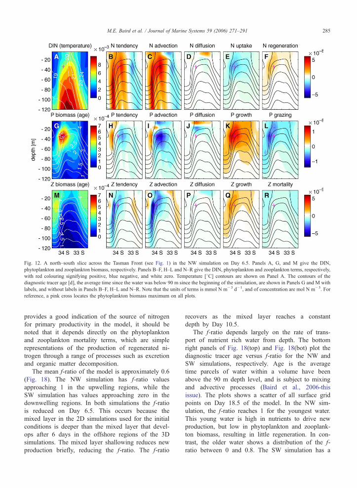
Fig. 12. A north–south slice across the Tasman Front (see Fig. 1) in the NW simulation on Day 6.5. Panels A, G, and M give the DIN,

phytoplankton and zooplankton biomass, respectively. Panels B–F, H–L and N–R give the DIN, phytoplankton and zooplankton terms, respectively,

with red colouring signifying positive, blue negative, and white zero. Temperature [8C] contours are shown on Panel A. The contours of the

diagnostic tracer age [d], the average time since the water was below 90 m since the beginning of the simulation, are shown in Panels G and M with

labels, and without labels in Panels B–F, H–L and N–R. Note that the units of terms is mmol N m�3 d�1, and of concentration are mol N m�3. For

reference, a pink cross locates the phytoplankton biomass maximum on all plots.


provides a good indication of the source of nitrogen

for primary productivity in the model, it should be

noted that it depends directly on the phytoplankton

and zooplankton mortality terms, which are simple

representations of the production of regenerated ni-

trogen through a range of processes such as excretion

and organic matter decomposition.

The mean f-ratio of the model is approximately 0.6

(Fig. 18). The NW simulation has f-ratio values

approaching 1 in the upwelling regions, while the

SW simulation has values approaching zero in the

downwelling regions. In both simulations the f-ratio

is reduced on Day 6.5. This occurs because the

mixed layer in the 2D simulations used for the initial

conditions is deeper than the mixed layer that devel-

ops after 6 days in the offshore regions of the 3D

simulations. The mixed layer shallowing reduces new

production briefly, reducing the f-ratio. The f-ratio

recovers as the mixed layer reaches a constant

depth by Day 10.5.

The f-ratio depends largely on the rate of trans-

port of nutrient rich water from depth. The bottom

right panels of Fig. 18(top) and Fig. 18(bot) plot the

diagnostic tracer age versus f-ratio for the NW and

SW simulations, respectively. Age is the average

time parcels of water within a volume have been

above the 90 m depth level, and is subject to mixing

and advective processes (Baird et al., 2006-this

issue). The plots shows a scatter of all surface grid

points on Day 18.5 of the model. In the NW sim-

ulation, the f-ratio reaches 1 for the youngest water.

This young water is high in nutrients to drive new

production, but low in phytoplankton and zooplank-

ton biomass, resulting in little regeneration. In con-

trast, the older water shows a distribution of the f-

ratio between 0 and 0.8. The SW simulation has a

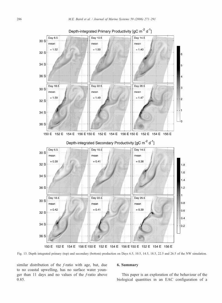
Fig. 13. Depth integrated primary (top) and secondary (bottom) production on Days 6.5, 10.5, 14.5, 18.5, 22.5 and 26.5 of the NW simulation.


similar distribution of the f-ratio with age, but, due

to no coastal upwelling, has no surface water youn-

ger than 11 days and no values of the f-ratio above

0.85.

6. Summary

This paper is an exploration of the behaviour of the

biological quantities in an EAC configuration of a

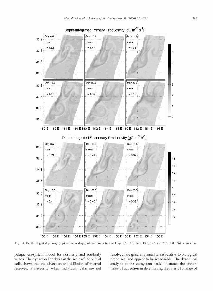
Fig. 14. Depth integrated primary (top) and secondary (bottom) production on Days 6.5, 10.5, 14.5, 18.5, 22.5 and 26.5 of the SW simulation.


pelagic ecosystem model for northerly and southerly

winds. The dynamical analysis at the scale of individual

cells shows that the advection and diffusion of internal

reserves, a necessity when individual cells are not

resolved, are generally small terms relative to biological

processes, and appear to be reasonable. The dynamical

analysis at the ecosystem scale illustrates the impor-

tance of advection in determining the rates of change of

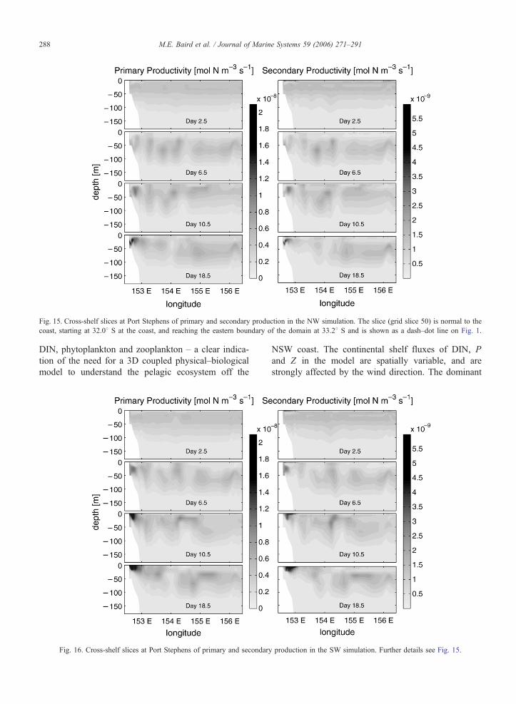
Fig. 15. Cross-shelf slices at Port Stephens of primary and secondary production in the NW simulation. The slice (grid slice 50) is normal to the

coast, starting at 32.08 S at the coast, and reaching the eastern boundary of the domain at 33.28 S and is shown as a dash–dot line on Fig. 1.


DIN, phytoplankton and zooplankton – a clear indica-

tion of the need for a 3D coupled physical–biological

model to understand the pelagic ecosystem off the

Fig. 16. Cross-shelf slices at Port Stephens of primary and secondary

NSW coast. The continental shelf fluxes of DIN, P

and Z in the model are spatially variable, and are

strongly affected by the wind direction. The dominant

production in the SW simulation. Further details see Fig. 15.

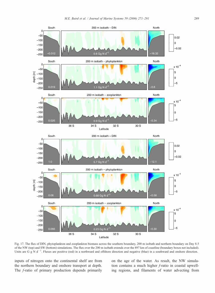
Fig. 17. The flux of DIN, phytoplankton and zooplankton biomass across the southern boundary, 200 m isobath and northern boundary on Day 8.5

of the NW (top) and SW (bottom) simulations. The flux over the 200 m isobath extends over the 897 km of coastline (boundary boxes not included).

Units are G g N d�1. Fluxes are positive (red) in a northward and offshore direction and negative (blue) in a southward and onshore direction.


inputs of nitrogen onto the continental shelf are from

the northern boundary and onshore transport at depth.

The f-ratio of primary production depends primarily

on the age of the water. As result, the NW simula-

tion contains a much higher f-ratio in coastal upwell-

ing regions, and filaments of water advecting from

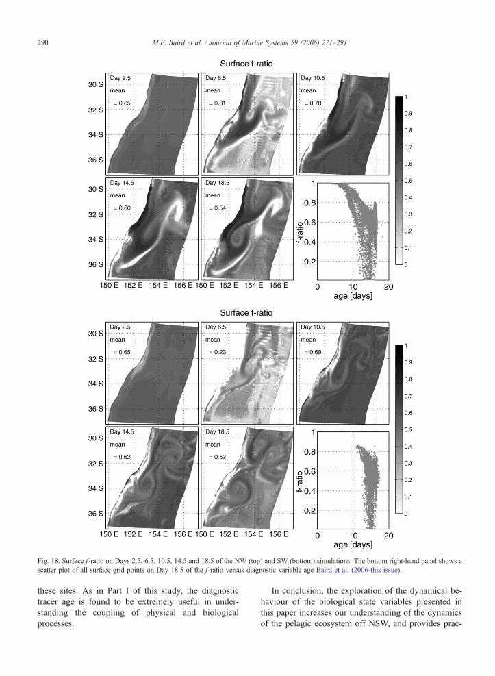
Fig. 18. Surface f-ratio on Days 2.5, 6.5, 10.5, 14.5 and 18.5 of the NW (top) and SW (bottom) simulations. The bottom right-hand panel shows a

scatter plot of all surface grid points on Day 18.5 of the f-ratio versus diagnostic variable age Baird et al. (2006-this issue).


these sites. As in Part I of this study, the diagnostic

tracer age is found to be extremely useful in under-

standing the coupling of physical and biological

processes.

In conclusion, the exploration of the dynamical be-

haviour of the biological state variables presented in

this paper increases our understanding of the dynamics

of the pelagic ecosystem off NSW, and provides prac-


tical outputs such as continental shelf fluxes. Future

work will be directed towards configuring the model to

simulate observed events off the NSW coast over an-

nual time-scales to estimate important biological ocean-

ographic phenomena such as annual productivity and

the transport of organic matter from the shelf regions to

the open ocean.

Acknowledgements

This research was funded by ARC Discovery Project

DP0209193 held by IS and MB and ARC Discovery

Project DP0208663 held by JM. The use of the Aus-

tralian Partnership for Advanced Computing (APAC)

supercomputer, and the scientific programming support

of Clinton Chee (High Performance Computing Unit,

UNSW) is gratefully acknowledged. We thank Alan

Blumberg and George Mellor for the free availability

of the Princeton Ocean Model, and Patrick Marche-

siello and Peter Oke for earlier work on the East

Australian Current configuration.

References

Baird, M.E., Middleton, J.H., 2004. On relating physical limits to the

carbon: nitrogen ratio of unicellular algae and benthic plants.

J. Mar. Syst. 49, 169–175.

Baird, M.E., Oke, P.R., Suthers, I.M., Middleton, J.H., 2004. A

plankton population model with bio-mechanical descriptions of

biological processes in an idealised 2-D ocean basin. J. Mar. Syst.

50, 199–222.

Baird, M.E., Timko, P.G., Suthers, I.M., Middleton, J.H., 2006-this

issue. Coupled physical-biological modelling study of the East

Australian Current with idealised wind forcing: Part I. Biological

model intercomparison. J. Mar. Syst. 59, 249–270. doi:10.1016/

j.jmarsys.2005.09.005.

Beckmann, A., Hense, I., 2004. Torn between extremes: the ups and

downs of phytoplankton. Ocean Dyn. 54, 581–592.

Behrenfeld, M.J., Falowski, P.G., 1997. A consumer’s guide to phy-

toplankton primary productivity models. Limnol. Oceanogr. 42,

1479–1491.

Blumberg, A.F., Mellor, G.L., 1987. A description of a three-dimen-

sional coastal ocean circulation model. In: Heaps, N. (Ed.), Three-

dimensional Coastal Ocean Models. American Geophysical

Union, pp. 1–15.

Craig, P.D., Banner, M.L., 1994. Modelling wave-enhanced turbulence

in the ocean surface layer. J. Phys. Oceanogr. 24, 2546–2559.

Dugdale, R.C., 1967. Nutrient limitation in the sea: dynamics, iden-

tification and significance. Limnol. Oceanogr. 12, 685–695.

Edwards, C.A., Batchelder, H.P., Powell, T.M., 2000. Modelling

microzooplankton and macrozooplankton dynamics within a

coastal upwelling system. J. Plankton. Res. 22, 1619–1648.

Eppley, R.W., Peterson, B.J., 1979. Particle organic matter flux and

planktonic new production in the deep ocean. Nature 282,

677–680.

Fasham, M.J.R., Ducklow, H.W., McKelvie, S.M., 1990. A nitrogen-

based model of plankton dynamics in the oceanic mixed layer.

J. Mar. Res. 48, 591–639.

Franks, P.J.S., Walstad, L.J., 1997. Phytoplankton patches at fronts: A

model of formation and response to wind events. J. Mar. Res. 55,

1–29.

Laundry, M.R., 2004. Microzooplankton production in the oceans.

ICES J. Mar. Sci. 61, 501–507.

Mesias, J.M.R.P.M., Strub, P.T., 2003. Dynamical analysis of the

upwelling circulation off central Chile. J. Geophys. Res. 108

(C3), 3085.

Oke, P.R., 2002. A modelling study of the three-dimensional conti-

nental shelf circulation off. Oregon, Part II. Dynamical analysis. J.

Phys. Oceanogr. 32, 1383–1403.

Yool, A., Fasham, M.J.R., 2001. An examination of the continental

shelf pump in an open ocean general circulation model. Global

Biogeochem. Cyc. 15, 831–844.

http://dx.doi.org/doi:10.1016/j.jmarsys.2005.09.005

Documents

Coupled physical–biological modelling study of the East