Coupled GPS/MEMS IMU Attitude Determination of Small UAVs

electronics

Article

Coupled GPS/MEMS IMU Attitude Determination ofSmall UAVs with COTSMichael Strohmeier * and Sergio Montenegro

Chair of Aerospace Information Technology, Julius-Maximillians-Universität Würzburg, Josef-Martin-Weg,97074 Würzburg, Germany; [email protected]* Correspondence: [email protected]; Tel.: +49-931-31-86192

Academic Editor: Mostafa BassiouniReceived: 15 December 2016; Accepted: 4 February 2017; Published: 10 February 2017

Abstract: This paper proposes an attitude determination system for small Unmanned Aerial Vehicles(UAV) with a weight limit of 5 kg and a small footprint of 0.5 m×0.5 m. The system is realized bycoupling single-frequency Global Positioning System (GPS) code and carrier-phase measurementswith the data acquired from a Micro-Electro-Mechanical System (MEMS) Inertial MeasurementUnit (IMU) using consumer-grade Components-Off-The-Shelf (COTS) only. The sensor fusion isaccomplished using two Extended Kalman Filters (EKF) that are coupled by exchanging informationabout the currently estimated baseline. With a baseline of 48 cm, the static heading accuracy of theproposed system is comparable to the one of a commercial single-frequency GPS heading systemwith an accuracy of approximately 0.25◦/m. Flight testing shows that the proposed system is able toobtain a reliable and stable GPS heading estimation without an aiding magnetometer.

Keywords: UAV; attitude determination; Attitude Heading Reference System (AHRS); GPS; Real-timeKinematics (RTK); MEMS IMU; magnetometer

1. Introduction

Within the Helmholtz Alliance for Robotic Exploration of Extreme Environments (ROBEX),small Unmanned Aerial Vehicles (UAVs) are developed to support an Autonomous UnderwaterVehicle (AUV) during explorations below Arctic sea ice. In order to operate the AUV successfully atthe marginal ice zone, it is crucial to keep track of the permanently-moving ice edge. By deployingGPS-based tracking devices at the ice edge, the ice drift can be continuously observed before and duringAUV operations. In a first attempt, the Alfred Wegener Institute for Polar and Marine Research (AWI)deployed suitable tracking systems manually at the ice edge using zodiacs and a radio-controlledUAV. However, the manual deployment of the tracking systems turned out to be dangerous and timeconsuming [1]. The UAV’s limited operation range was identified as a major disadvantage and createdthe demand for more autonomous UAVs in Arctic environments.

While a variety of consumer-grade and professional solutions for autonomous UAVs exists,the Arctic environment is still a challenge for small autonomous UAVs. One critical aspect is areliable heading estimation despite the weak horizontal component of the Earth’s magnetic field inhigh latitudes. A reliable approach to determine the vehicle heading in the presence of magneticdisturbances is to estimate the relative position between several Global Navigation Satellite System(GNSS) receivers. Typical GNSS attitude determination systems consist of two or more GNSS receiversthat are deployed on a moving platform at a sufficiently large distance from each other. The so-calledbaselines usually range from 1 m for cars up to 40 m or more for aircraft and ships [2–5]. However,smaller baselines down to 2–3 L1 carrier wavelengths (L1 = 1575.42 MHz) are also possible [6]. In orderto obtain the required measurement accuracy, carrier-phase observations are used. Usually, thoseobservations are strongly influenced by error terms, such as tropospheric and ionospheric delay,

Electronics 2017, 6, 15; doi:10.3390/electronics6010015 www.mdpi.com/journal/electronics

http://www.mdpi.com/journal/electronics

http://www.mdpi.com

http://www.mdpi.com/journal/electronics

Electronics 2017, 6, 15 2 of 18

receiver clock errors, multi-path errors and receiver noise. However, by calculating Single-Difference(SD) between receivers and Double-Difference (DD) between receivers and satellites, some of the errorterms in the carrier-phase observation can be eliminated.

Already in the early 1990s, research on GPS-based attitude determination for aircraft wasconducted and successfully tested in flight [7,8]. Since then, systems based on high-end dual-frequency(L1 and L2 band) GNSS receivers emerged as the state of the art solution. However, the upcomingof inexpensive MEMS inertial sensors and the growing demand of small UAVs for various tasksencouraged the development of less expensive GNSS attitude determination systems.

Concoli et al. [9] describe the use of multi-GNSS receivers for the attitude determination of a UAVon a conceptional level and simulate the influence of different baseline length.

Falco et al. [10] describe an approach for their 1.5 m×1.5 m footprint UAV based on an array offour single-frequency GPS receivers combined with a consumer-grade MEMS IMU. In their approach,DDs are exploited to calculate the attitude. The heading angle was estimated during a UAV flighttest with a mean error below one degree using a short baseline array of 50 cm×50 cm. The navigationsystem was implemented on the LOGAM platform, a customized board with four GNSS receivers,an IMU, a barometer and a micro-controller. Since no details about the used components are given,a full price for the system cannot be estimated. However, the price for the four utilized Bullet IIIantennas is about 350$.

Eling et al. [11] combine the measurements of a tactical-grade IMU (ADIS16488) witha dual-frequency (Novatel OEM 615) and a single-frequency (u-Blox Lea6T) GPS receiver.The processing was performed on the National Instruments embedded processing platform sbRIO9606.The dual-frequency receiver is used for the absolute positioning and as one receiver for the movingbaseline. The single-frequency receiver is used as the second baseline receiver. With a baseline of 92 cm,a heading accuracy of 0.2◦ can be achieved. Two geodetic-grade antennas (3G + C, navXperience)were used. Using tactical- to geodetic-grade only, the total system costs are very high compared to thesolution proposed in this article.

This article will focus on the GPS/IMU-based attitude determination of a small UAV witha take-off weight of less than 5 kg and a very small footprint of 0.5 m×0.5 m using low-cost,consumer-grade COTS only. The total costs for the proposed navigation system are less than 400$.The system is compared to the commercial Static Heading Determination System from ANavS andtested during flight.

2. System Architecture

The attitude determination system in this approach is based on two single-frequencyGNSS receivers (Neo-M8T; u-Blox, Thalwil, Switzerland) with active low-cost patch antennas, aconsumer-grade MEMS IMU (LSM9DS0; STMicroelectronics, Geneva, Switzerland) and an embeddedprocessing platform (UDOO Neo; Seco, Arezzo, Italy). The system combines the carrier-phase ofthe L1 frequency GPS signal, the GPS pseudo-ranges, as well as the accelerometer, magnetometerand gyroscope measurements of the IMU using Real-Time Kinematics (RTK). Figure 1 shows theUAV concept.

The origin of the UAV fixed body frame is in its center of mass; the origin of the RTK frame is fixedto one of the GPS antennas, as shown in the figure. The GPS antennas are mounted on the UAV boomsat a distance of 48 cm, while the IMU is mounted in the UAV’s center of mass. The misalignment errordue to installation imprecisions between the IMU and GPS antennas is considered to be very smalland therefore neglected.


Figure 1. Unmanned Aerial Vehicle (UAV) concept with mounted Global Positioning System (GPS)antennas and important coordinate frames.

The matrix Rbr to rotate a vector from the body in the RTK frame is given by:

Rbr =

0 −1 0−1 0 00 0 −1

(1)

The UAV autopilot and its attitude determination system are based on the UDOO Neo. The UDOONeo incorporates an i.MX6 SoloX, a heterogeneous dual-core processor from NXP. The processorfeatures an ARM Cortex-A9 running at 1 GHz and an ARM Cortex-M4 at 200 MHz in one chip andallows inter-core communication using shared memory. The A9 core is running Linux and the RobotOperating System (ROS) [12]. The M4 core is running the Real-time Onboard Dependable OperatingSystem (RODOS) [13]. Therefore, the bigger core is used for computationally heavy tasks with softreal-time requirements, like the GPS heading estimation, while the small core handles firm real-timetasks, such as high-frequency attitude determination and attitude control. The computational tasks forthe attitude determination of the system are distributed among both processors, as shown in Figure 2.

QuaternionExtendedKalman

Filter

Gyro

Accel

Mag

C

C′

Real-TimeKinematics

Rover

Base

WMM

yg

ya

ym

qnb

γGPS

∆xn

∆xn

Φir, Pi

r

Φib, Pi

b

δ

δ

λ, ϕ

IMU

GPS

Cortex-M4

Cortex-A9

Figure 2. Proposed attitude determination system.


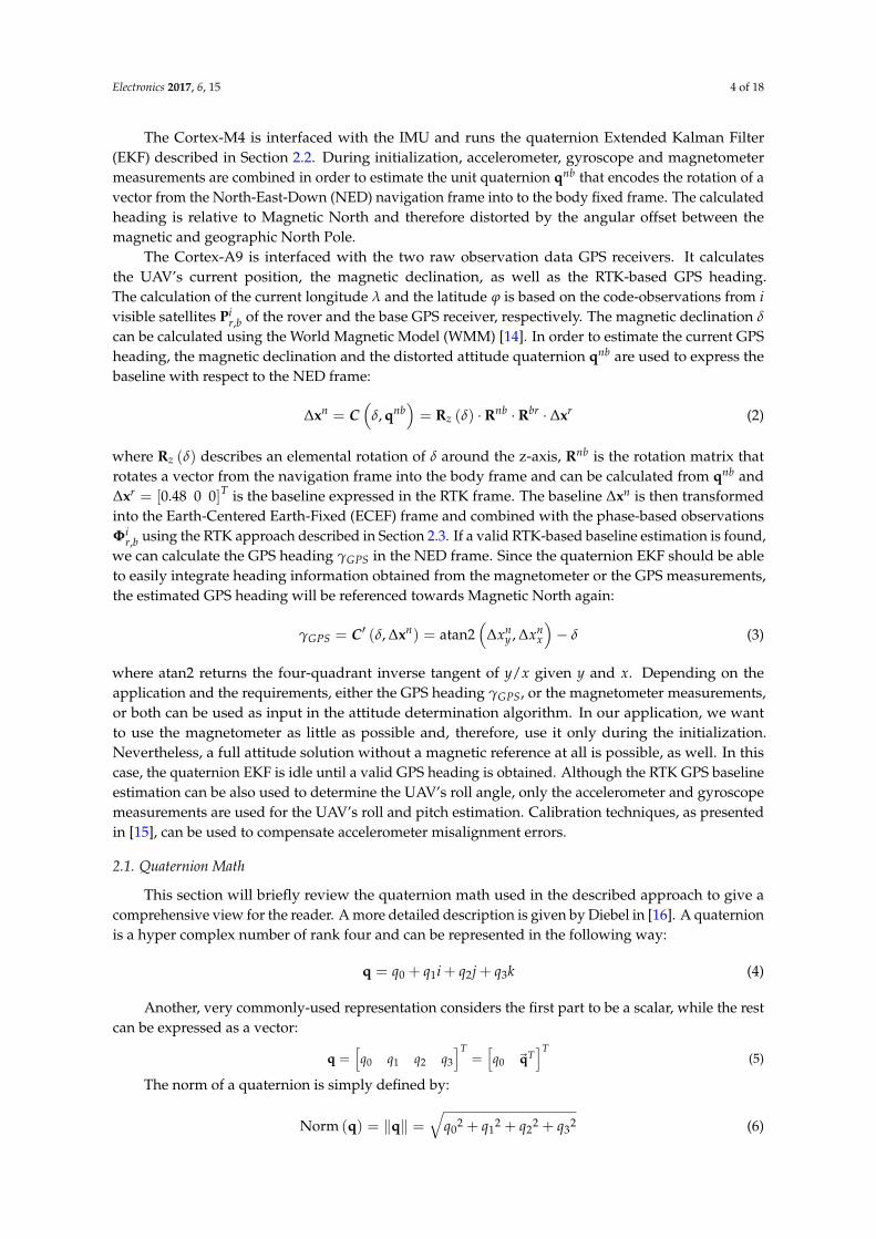
The Cortex-M4 is interfaced with the IMU and runs the quaternion Extended Kalman Filter(EKF) described in Section 2.2. During initialization, accelerometer, gyroscope and magnetometermeasurements are combined in order to estimate the unit quaternion qnb that encodes the rotation of avector from the North-East-Down (NED) navigation frame into to the body fixed frame. The calculatedheading is relative to Magnetic North and therefore distorted by the angular offset between themagnetic and geographic North Pole.

The Cortex-A9 is interfaced with the two raw observation data GPS receivers. It calculatesthe UAV’s current position, the magnetic declination, as well as the RTK-based GPS heading.The calculation of the current longitude λ and the latitude ϕ is based on the code-observations from ivisible satellites Pi

r,b of the rover and the base GPS receiver, respectively. The magnetic declination δ

can be calculated using the World Magnetic Model (WMM) [14]. In order to estimate the current GPSheading, the magnetic declination and the distorted attitude quaternion qnb are used to express thebaseline with respect to the NED frame:

∆xn = C(

δ, qnb)= Rz (δ) ·Rnb ·Rbr · ∆xr (2)

where Rz (δ) describes an elemental rotation of δ around the z-axis, Rnb is the rotation matrix thatrotates a vector from the navigation frame into the body frame and can be calculated from qnb and∆xr = [0.48 0 0]T is the baseline expressed in the RTK frame. The baseline ∆xn is then transformedinto the Earth-Centered Earth-Fixed (ECEF) frame and combined with the phase-based observationsΦi

r,b using the RTK approach described in Section 2.3. If a valid RTK-based baseline estimation is found,we can calculate the GPS heading γGPS in the NED frame. Since the quaternion EKF should be ableto easily integrate heading information obtained from the magnetometer or the GPS measurements,the estimated GPS heading will be referenced towards Magnetic North again:

γGPS = C′ (δ, ∆xn) = atan2(

∆xny , ∆xn

x

)− δ (3)

where atan2 returns the four-quadrant inverse tangent of y/x given y and x. Depending on theapplication and the requirements, either the GPS heading γGPS, or the magnetometer measurements,or both can be used as input in the attitude determination algorithm. In our application, we wantto use the magnetometer as little as possible and, therefore, use it only during the initialization.Nevertheless, a full attitude solution without a magnetic reference at all is possible, as well. In thiscase, the quaternion EKF is idle until a valid GPS heading is obtained. Although the RTK GPS baselineestimation can be also used to determine the UAV’s roll angle, only the accelerometer and gyroscopemeasurements are used for the UAV’s roll and pitch estimation. Calibration techniques, as presentedin [15], can be used to compensate accelerometer misalignment errors.

2.1. Quaternion Math

This section will briefly review the quaternion math used in the described approach to give acomprehensive view for the reader. A more detailed description is given by Diebel in [16]. A quaternionis a hyper complex number of rank four and can be represented in the following way:

q = q0 + q1i + q2j + q3k (4)

Another, very commonly-used representation considers the first part to be a scalar, while the restcan be expressed as a vector:

q =[q0 q1 q2 q3

]T=[q0 ~qT

]T(5)

The norm of a quaternion is simply defined by:

Norm (q) = ‖q‖ =√

q02 + q12 + q22 + q32 (6)


The conjugate of quaternion q can be obtained by negating its vector part and is denoted by q∗:

Conj (q) = q∗ =[q0 −~qT

]T(7)

Unit quaternions can be used to describe rotations in three-dimensional space. For the specialcase of a unitary quaternion, the inverse of the quaternion equals its conjugate:

Inv (q) = q−1 =q∗

‖q‖2 (8)

The product of two quaternions q and p is calculated using the Kronecker product and denotedwith ⊗ . Two subsequent rotations q and p can be expressed in a single rotation by multiplying bothquaternions. It is important to mention that the quaternion multiplication is not commutative.

The quaternion multiplication can therefore be denoted as:

q⊗ p =

[q0 p0 −~q ·~p

q0~p + p0~q +~q×~p

]

=

q0 −q1 −q2 −q3

q1 q0 −q3 q2

q2 q3 q0 −q1

q3 −q2 q1 q0

p0

p1

p2

p3

= Q(q)p

(9)

If a measurement of the rotational velocity in the body frame ωb and a quaternion q that describesthe rotation of a vector from the fixed navigation frame into the body frame are given, we can easilycalculate the quaternion’s derivative q with:

q =12

q⊗[

0ωb

]=

12

Q(q)

[0

ωb

](10)

A vector v given in three-dimensional space can be simply rotated from a fixed frame to a bodyframe, given that the rotation between the two frames is described by q, with:[

0w

]= q ⊗

[0v

]⊗ q∗ (11)

The same rotation can be obtained by expressing the quaternion q as a rotation matrix from thefixed frame n to the body frame b with:

w = Rnbv =

q02 + q1

2 − q22 − q3

2 2 (q1q2 − q0q3) 2 (q0q2 + q1q3)

2 (q1q2 + q0q3) q02 − q1

2 + q22 − q3

2 2 (q2q3 − q0q1)

2 (q1q3 − q0q2) 2 (q0q1 + q2q3) q02 − q1

2 − q22 + q3

2

~v (12)

For a more convenient way to interpret quaternions, they can be converted to Euler angles usingthe following equation: Φ

ΘΨ

=

atan2(2 (q0q1 + q2q3) , 1− 2

(q1

2 + q22))

asin (2 (q0q2 − q1q3))

atan2(2 (q0q3 + q1q2) , 1− 2

(q2

2 + q32)) (13)


2.2. Quaternion Extended Kalman Filter

The IMU measurements are combined with the GPS heading estimation in an EKF.The implemented filter is based on the approach used by Munguia et al. [17], but is augmentedby the RTK GPS heading and designed in such a way that update steps with different sensor ratesare possible.

2.2.1. Measurement Models

The IMU consists of a three-axis gyroscope, a three-axis accelerometer and a three-axismagnetometer. The gyroscope measurement vector yg consists of the angular rate in the body frameωb and additive errors that can be modeled by:

yg = ωb + bg + υg (14)

where bg is the temperature-dependent gyro bias and υg is Gaussian white noise with a variance ofσg

2. The accelerometer measurement vector ya is defined by:

ya = ab − gb + ba + υa (15)

where ab is the device acceleration in the body frame, gb is the gravity vector expressed in the bodyframe, ba is the accelerometer bias and υa is Gaussian white noise with a variance of σa

2. Since thebias in the accelerometer triads can be minimized through proper calibration methods [15], it will beneglected in this filter.

The magnetometer measurement vector ym can be described as:

ym = mb + bm + υm (16)

where mb is the surrounding magnetic field, bm is a constant magnetometer bias and υm is Gaussianwhite noise with a variance of σm

2. The magnetometer bias bm can be compensated for by estimatingthe so-called hard and soft iron effects using appropriate calibration methods as presented in [18].Ideally, the surrounding magnetic field mb is identical to the Earth’s magnetic field. However, metalstructures close to the magnetometer, as well as changing currents in the proximity of the magnetometerdisturb the Earth’s magnetic field. Compensating for those errors is a very challenging task and notalways possible. For simplicity, mb is assumed to be identical to the Earth’s magnetic field in thisfilter design.

Finally, the RTK GPS heading measurement yGPS is modeled by:

yGPS = γGPS + υGPS (17)

where γGPS describes the north heading referenced to the magnetic pole, in order to allow easierintegration of GPS heading and magnetometer measurements, and υGPS is Gaussian white noise witha variance of σGPS

2.

2.2.2. System Propagation

The system state x(k|k) at the time k is given by:

x(k|k) =[qnb(k|k)T

ωb(k|k)Tbg(k|k)

T]T

(18)

where qnb is a unit quaternion representing the orientation of the UAV fixed body frame with respectto the navigation frame and ωb and bg are defined according to Equation (14).


The system state can be predicted at fixed rate ∆t with the following propagation model:

x(k + 1|k) = f(

k, x(k|k), yg(k|k))=

qnb + ∆t · 1

2qnb ⊗

[0

ωb

]︸︷︷︸

qnb

yg − bg(1− λxg · ∆t

)bg

(19)

where qnb is the quaternion derivative and λxg is a time correlation factor that models how fast thegyroscope bias bg can vary.

The system state covariance matrix P can be propagated by:

P(k + 1|k) = ∇FxP(k|k)∇FxT + Q (20)

where ∇Fx is the Jacobian of the system prediction function f and Q is the system noise covariancematrix. The Jacobian of the system prediction function is evaluated for the latest state estimate andgiven by:

∇Fx =∂ f (k)

∂x

∣∣∣∣x=x(k|k)

(21)

The system noise covariance matrix can be expressed as:

Q =

04×4 0 00 σg

2 · I3×3 00 0 σbg

2 · I3×3

(22)

where σg2 is defined according to Equation (14) and σbg

2 is the variance of the gyroscope bias.

2.2.3. System Updates

The filter is designed in such a way that measurement updates can occur independently fromeach other. While the system state is propagated at fixed intervals of 5 ms, the accelerometer updatesoccur only if the body is not accelerating. The magnetometer measurements are only used as long asno valid GPS heading is available, and the GPS heading is integrated at 10 Hz as soon as it is computedby the RTK GPS heading estimation. The measurement update for the system state and the systemstate covariance is given by the following equations:

x(k + 1|k + 1) = x(k + 1|k) + W (zi − zi) (23)

P(k + 1|k + 1) = P(k + 1|k) + WSiWT (24)

where zi is the current measurement and zi is the measurement prediction. W is the Kalman filter gain,and Si is the residual covariance matrix. i describes the sensor used for the particular measurementupdate and can be summarized as i ∈ {a, γm, γGPS}: a represents the accelerometer measurementupdate, γm the yaw angle update based on the magnetometer and γGPS the yaw angle update basedon the estimated GPS heading. The residual covariance matrix Si can be calculated by:

Si = ∇HiP(k + 1|k)∇HiT + Ri (25)

where∇Hi is the Jacobian of the respective measurement prediction model hi evaluated for the currentsystem state prediction:

∇Hi =∂hi(k + 1)

∂x

∣∣∣∣x=x(k+1|k)

(26)


Finally, the Kalman filter gain is given by:

W = P(k + 1|k)∇HiTSi−1 (27)

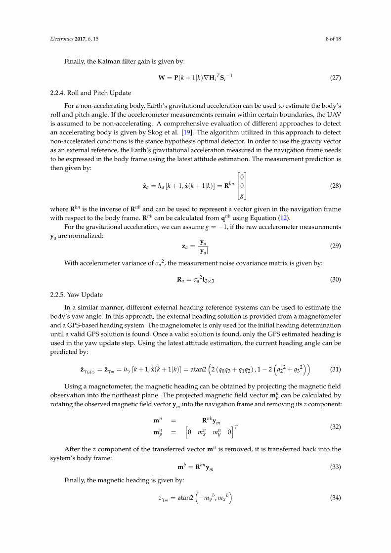
2.2.4. Roll and Pitch Update

For a non-accelerating body, Earth’s gravitational acceleration can be used to estimate the body’sroll and pitch angle. If the accelerometer measurements remain within certain boundaries, the UAVis assumed to be non-accelerating. A comprehensive evaluation of different approaches to detectan accelerating body is given by Skog et al. [19]. The algorithm utilized in this approach to detectnon-accelerated conditions is the stance hypothesis optimal detector. In order to use the gravity vectoras an external reference, the Earth’s gravitational acceleration measured in the navigation frame needsto be expressed in the body frame using the latest attitude estimation. The measurement prediction isthen given by:

za = ha [k + 1, x(k + 1|k)] = Rbn

00g

(28)

where Rbn is the inverse of Rnb and can be used to represent a vector given in the navigation framewith respect to the body frame. Rnb can be calculated from qnb using Equation (12).

For the gravitational acceleration, we can assume g = −1, if the raw accelerometer measurementsya are normalized:

za =ya|ya|

(29)

With accelerometer variance of σa2, the measurement noise covariance matrix is given by:

Ra = σa2I3×3 (30)

2.2.5. Yaw Update

In a similar manner, different external heading reference systems can be used to estimate thebody’s yaw angle. In this approach, the external heading solution is provided from a magnetometerand a GPS-based heading system. The magnetometer is only used for the initial heading determinationuntil a valid GPS solution is found. Once a valid solution is found, only the GPS estimated heading isused in the yaw update step. Using the latest attitude estimation, the current heading angle can bepredicted by:

zγGPS = zγm = hγ [k + 1, x(k + 1|k)] = atan2(

2 (q0q3 + q1q2) , 1− 2(

q22 + q3

2))

(31)

Using a magnetometer, the magnetic heading can be obtained by projecting the magnetic fieldobservation into the northeast plane. The projected magnetic field vector mn

p can be calculated byrotating the observed magnetic field vector ym into the navigation frame and removing its z component:

mn = Rnbym

mnp =

[0 mn

x mny 0

]T (32)

After the z component of the transferred vector mn is removed, it is transferred back into thesystem’s body frame:

mb = Rbnym (33)

Finally, the magnetic heading is given by:

zγm = atan2(−my

b, mxb)

(34)


Using a GPS heading reference system that provides the Magnetic North heading as output,the GPS yaw measurement is simply obtained by:

zγGPS = γGPS (35)

In both cases, for the GPS and the magnetic reference system, the yaw measurements zγj areassumed to have Gaussian white noise with a variance of σγj

2 where j ∈ {m, GPS}. The accordingmeasurement noise covariance matrices are therefore given by:

Rγj = σγj2 (36)

Similar to the non-accelerating body detection for the roll and pitch update, invalid GPSmeasurements have to be detected and should not be integrated into the final attitude estimation of thequaternion EKF. Two criteria are applied at every GPS yaw update step in order to validate whetherthe estimated RTK GPS heading is reliable or not. First, the length of the estimated baseline has to bewithin an acceptable range if compared to the a priori known value, and second, the GPS headingmust be based on an integer fixed solution.

During filter initialization, the sampling variance is additionally compared to the expectedvariance of the GPS heading in a static scenario. The GPS/IMU sensor fusion will be only started ifthe observed sampling variance is below a fixed threshold.

2.3. Real-Time Kinematics

The GPS heading estimation system is combining code measurements, carrier-phasemeasurements, the a priori known baseline length and the current baseline orientation in an EKF.The filter approach is based on the open source Real-Time Kinematics Library (RTKLIB) by Takasu [20],but augmented by the baseline orientation measurement and, therefore, the IMU coupling. The EKFtries to estimate the position and velocity of one antenna (rover) relative to the other antenna (base),as well as the carrier-phase ambiguity float solutions. The obtained float solutions are then resolved intofixed integer solutions. Once a valid three-dimensional baseline estimation is calculated, its headingcan be easily derived.

Since only L1 carrier-phase signals are considered, the measurement models for the DD carrierphase Φ

ijrb and the DD pseudo ranges Pij

rb are given by:

Φijrb = ρ

ijrb + λ1

(Bi

rb,1 − Bjrb,1

)+ εΦ (37)

Pijrb = ρ

ijrb + εP (38)

where ρijrb is the geometric range DD, λ1 is the L1 carrier wavelength and εΦ,P are the carrier phase

and pseudo range measurement errors, respectively. In order to avoid the hand-over problems whenthe reference satellite is changing [20], internally Single-Difference ambiguities Bi

rb,1 are used instead

of Double-Difference ambiguities Bijrb,1. The system state for the EKF is therefore given by:

x(k|k) =[rr(k|k)T vr(k|k)T Bi

rb,1(k|k)T]T

(39)

where rr and vr are the rover position and velocity, respectively. The system state and its covariancecan be predicted by:

x(k + 1|k) = Fx(k|k) (40)

P(k + 1|k) = ∇FP(k|k)∇FT + Q (41)


The system propagation matrix F and the system noise covariance Q are given by:

F =

I3×3 ∆t · I3×3 00 I3×3 00 0 Im×m

, Q =

03×3 0 00 Qv 00 0 0m×m

(42)

where ∆t is the sample time of the GPS receiver and with:

Qv = RenTdiag(

σ2vn∆t, σ2

ve∆t, σ2vd∆t

)Ren (43)

where Ren describes a rotation matrix from the ECEF frame into the local coordinate frame (NED) atthe receiver antenna position and σvn, σve and σvd are the standard deviations of the rover velocity innorth, east and down direction, respectively.

The measurement vector in RTKLIB consists of the baseline length |∆xe|, the DD carrier-phasemeasurements Φ

ijrb and the DD pseudo-range measurements Pij

rb, where the subscript r is the rover, thesubscript b is the base, the superscript j is the reference satellite and the superscript i ∈ {1, 2, . . . , m} isthe number of valid DD measurements. This measurement vector is extended by ∆xe, the baselinevector in the ECEF frame, and thus reads:

z =[Φi1

rb . . . Φimrb Pi1

rb . . . Pimrb |∆xe| ∆xeT

]T(44)

The measurement update equations for the system state and the system state covariances aresimilar to the quaternion EKF approach and can be derived from Equations (23)–(27).

The measurement prediction matrix is given by:

z = h [k + 1, x(k + 1|k)] =

hΦrb,1

hPrb,1

h∆xe

h|∆xe |

=

hΦrb,1

hPrb,1

rr − rb|rr − rb|

(45)

where rb is the code-based calculated single position of the base antenna and hΦrb,1 and hPrb,1 depend

on the DD geometric range ρijrb,1 and L1 the carrier wavelength λ1 as follows:

hΦrb,1 =

ρi1

rb,1 + λ1

(Bi

rb,1 − B1rb,1

)ρi2

rb,1 + λ1

(Bi

rb,1 − B2rb,1

)...

ρimrb,1 + λ1

(Bi

rb,1 − Bmrb,1

)

, hPrb,1 =

ρi1

rb,1ρi2

rb,1...

ρimrb,1

(46)

This yields the following measurement Jacobian matrix:

H =

−DE 0 λ1D−DE 0 0(rr−rb)

T

|rr−rb |0 0

I3×3 0 0

, D =

1 −1...

. . .1 −1

(47)


where D is the double differencing matrix and E = (e1r , e2

r , ..., emr )

T describes the line of sight vectors fromthe rover antenna to the satellite i ∈ {1, 2, . . . , m}. Finally, the measurement noise matrix R is given by:

R =

DΣΦDT 0 0 0

0 DΣPDT 0 00 0 σ|∆xe|

2 00 0 0 Σ∆xe

(48)

where ΣΦ,P = diag(σ1Φ,P

2, . . . , σmΦ,P

2) describes the variances of the carrier-phase and the pseudo-rangemeasurements, respectively. σ|∆xe| is the accuracy of the a priori known baseline length and Σ∆xe theaccuracy of the estimated baseline orientation using the IMU coupling given by:

Σ∆xe = RenTdiag(

σn2, σe

2, σd2)

Ren (49)

where σn2, σe

2, σd2 describe the accuracy of the IMU baseline estimation in the NED frame.

The results of this measurement update are real-valued DD ambiguities. Fixing these real-valuedambiguities to integers improves the quality of the solution significantly. The integer ambiguityresolution is done for each measurement instantaneously using the MLAMBDAmethod [21]. At thispoint, it should be pointed out that the baseline length constraint, as well as the baseline orientationconstraint are used iteratively when estimating the float solution. No additional baseline constraintsare applied during the integer fixing step, as is the case for the baseline-constraint LAMBDA methodproposed by [22].

Once the integer ambiguities are fixed, the RTK-based baseline estimation in the ECEF frame issimply given by:

∆xe = rr(k + 1|k + 1)− rb(k + 1|k + 1); (50)

Using our current position estimate, this can be simply transformed into the NED frame.

3. Evaluation

In order to validate the performance of the proposed approach, various experiments wereconducted using a real-world system. All experiments were carried out on the UAV platform shown inFigure 3. The experiments were performed in Würzburg, Germany, on different days. To increase thequality of the GPS raw measurements, ground planes were used to reduce multipath effects as suggestedby [23]. The GPS raw measurements were obtained at 10 Hz, while the IMU provided data at 200 Hz.

Figure 3. The ROBEX UAV.


The following section will discuss two of the tested scenarios in detail with the focus on theaccuracy of the heading determination. Therefore, the system is first compared to other available GPSheading solutions in a static scenario. Subsequently, the system is evaluated during flight, covering thetypical dynamic range of the system.

3.1. Static Evaluation

In the static scenario, the proposed method is compared to the results of the RTKLIB only and acommercial system, the Static Heading Determination System from ANavS. The results of the ANavSsystem are considered to be the ground truth. The proposed algorithm is implemented on the UAVitself, and the here presented data are calculated on-board in real time while the results for the tworeferences systems were obtained by post-processing the recorded raw data. The proposed method iscompared to the ANavS reference system in Figure 4 for the total experiment duration. After a shortinitialization time, both systems provide a valid, stable and accurate heading solution. Although theUAV was placed on a field with a sufficient distance to trees and buildings in the attempt to provide aclear view of the sky for both GPS antennas for this experiment, two satellites’ locks were temporarilylost during the measurement. The impact of the loss of the two satellite signals can be clearly seenafter approximately 251 s. No valid reference heading could be provided during this time.

time [s]

0 50 100 150 200 250 300 350 400 450 500

Φ [°

]

-30

-20

-10

0

10

ANavS

QEKF/RTK

Figure 4. Static evaluation: the ANavS reference heading and the result of the proposed method.

Comparing the system precision, it can be seen that the combined GPS/IMU approach has muchlower noise than the reference solution. Table 1 lists the measured standard deviations during thisstatic scenario for the ANavS reference system, the proposed method and its RTK GPS-only solution, aswell as the standard RTKLIB solution. The standard deviations are calculated for the time between thefirst fix of all systems (t = 45 s) until the two satellite locks are lost (t = 245 s). Due to the combinationof the high data rate IMU and the RTK GPS heading, the system precision is significantly improved bythe quaternion EKF.

Table 1. Standard deviations during the static scenario.

System ANavS QEKF/RTK RTK RTKLIB

σ 0.37◦ 0.039◦ 0.30◦ 0.35◦

Figure 5 shows the progress of the yaw estimates for the different systems from a cold start untilfixed integer solutions are obtained. All systems obtain a valid solution after less than 45 s.

The reference system from ANavS does not provide any heading information until thecarrier-phase integer ambiguities are fixed and a possible solution is found. The time until thefirst heading estimation is provided takes under open-sky conditions approximately 15 s. During thefirst 30 s, the orbital data of the GPS satellites are gathered.

The proposed system is initialized based on the observed magnetic heading. In addition to theoverall system output, the RTK GPS heading estimates are also shown. Thereby, a comparison betweenthe different systems can be done in a more convenient way. After the orbital data are collected,


the integer ambiguities are fixed for every epoch using the baseline length and its currently-estimatedorientation. The jump after approximately 21 s indicates the moment when enough orbital data are acquiredto estimate the receiver position, and the WMM declination corrections can be applied. In this scenario, thefirst correct ambiguity fix is obtained after 123 epochs, which equals 12.3 s. Nevertheless, it takes someadditional time for the quaternion EKF to adapt the gyroscope biases and adjust its heading estimation.

time [s]

0 10 20 30 40 50 60

Φ [

°]

-30

-25

-20

-15

-10

-5

0

5

10

15

20

ANavS

QEKF/RTK

RTK

RTKLIB

Figure 5. Time to first fix: the reference system from ANavS, the proposed method and its GPSheading measurements and the GPS heading acquired from the RTKLIB using its standard settings fora moving baseline.

As a second reference, the initialization of RTKLIB’s static heading estimation only is also shownin Figure 5. The data are obtained using the RTKLIB default settings for a moving baseline of 48 cm.Using the RTKLIB’s fix and hold approach for the integer ambiguities, the first correct heading isestimated 19.8 s after the orbital data are obtained.

Figure 6 shows the impact of the aforementioned loss of satellite lock in more detail.After approximately 251 s, the signal of two satellite locks was lost presumably by accidentally shieldingthe GPS antennas in a specific direction.

time [s]

230 240 250 260 270 280 290

Φ [°

]

-30

-25

-20

-15

-10

-5

0

5

10

15

20

ANavS

QEKF/RTK

RTK

RTKLib

Figure 6. Temporary loss of the lock of two satellites: The reference system from ANavS, the proposedmethod and its GPS heading measurements and the GPS heading acquired from the RTKLIB using itsstandard settings for a moving baseline.


Figure 7 shows the Signal-to-Noise Ratio (SNR) of the tracked satellites during the satellite lossfor one of the GPS receivers. In total, eight satellites are tracked. The SNR of Satellites G27 and G32drops below 28 dB after 251 s and recovers again after approximately 15 s. Additionally, the signalstrength of the four other satellites is decreased during this time.

time [s]

230 240 250 260 270 280 290

SN

R [

dB

]

10

15

20

25

30

35

40

45

50

G01

G08

G10

G11

G18

G22

G27

G32

Figure 7. Tracked satellites of Receiver 2 during the static experiment: eight satellites are tracked; theSNR of Satellites G27 and G32 drops below 28 dB at t ≈ 251 s.

Although shielding is a very unlikely scenario for the final application, the reaction of the differentsystems is quite interesting. While the commercial system re-obtains a valid heading first at t ≈ 265 s,there are strong fluctuations and a temporary error of 20 degrees. In contrast to that, the proposedmethod takes admittedly longer to re-obtain a correct fix (t ≈ 275 s). However, the maximum errorof the proposed method remains under five degrees due to the IMU stabilization. Additionally, nosudden fluctuations can be observed, allowing a more stable flight. In contrast, the RTKLIB solutiondoes not manage to obtain a valid GPS heading again.

During the satellite loss, the measurements of the IMU and the RTK GPS heading are contradictingeach other. While the gyroscope measurements correctly indicate no change in orientation, the GPSheading indicates a change. Instead of trusting the GPS heading blindly, the gyroscope biases areadapted according to the time correlation factor λxg in Equation (19), while the IMU estimated baselineorientation constraint allows one to keep the RTK GPS heading stable.

3.2. Dynamic Evaluation

In the second scenario, the proposed system is tested during flight. After the initial GPS fix isobtained, the UAV takes off and hovers at a height of 5 m for several seconds. Next, the UAV flies in aclock-wards circle of approximately 11 m in diameter while facing away from the circle center. Thecircle is completed after 30 s. Subsequently, the UAV moves up and down at roughly the same positionwithout changing its heading. The recorded raw GPS positions of one receiver are shown in Figure 8.


East [m]

-10 -5 0 5 10 15 20

Nort

h [m

]

-15

-10

-5

0

5

Figure 8. Two-dimensional position during the evaluation flight.

The upper plot in Figure 9 shows the estimated heading during the flight. Again, in addition tothe overall system output, the GPS heading estimates are shown. Furthermore, the heading calculatedby post-processing the recorded data from the IMU and the magnetometer measurements is displayed,as well. Since the ANavS system is designed for static applications and due to the lack of a lightweightreference system that can be mounted on the UAV platform, the magnetic heading during flight isconsidered as the ground truth. It shall be noted that the magnetic heading is error-prone due tomagnetic disturbances by the UAV’s motors during flight and therefore can only provide an accuracyof a few degrees. Nevertheless, it can still be used to verify the functionality of the proposed methodin flight.

0 50 100 150

Ya

w [

°]

-200

-150

-100

-50

0

50

100

150

200

QEKF/MAG

QEKF/RTK

RTK

Time [s]

0 50 100 1500

0.5

1

Figure 9. Heading estimation during flight: magnetic- and GPS-based solution; update criteria.


The time until all orbit data are gathered takes again roughly 30 s. In contrast to the staticevaluation, an integer ambiguity fix could be obtained immediately with the first measurement. Bothsystems show a smooth circular heading estimation and remain constant once the circular flight iscompleted. The differences between the magnetic and the GPS-based heading can be caused by thepoor calibration of the constant magnetic offsets and the aforementioned additional time-varyingmagnetic effects, e.g., high electrical currents in the sensor vicinity due to the UAV operation. Thelower plot shows whether the update criteria for the yaw update are met or not (see Section 2.2.5) andindicate therefore if the estimated RTK GPS heading is used in the quaternion EKF.

4. Conclusions

This paper presents a method that allows an autonomous UAV to navigate during flightindependently of magnetic field measurements. The proposed method combines single-frequencyL1 GPS measurements with the measurements of a consumer-grade MEMS IMU. The sensorfusion is accomplished by using two EKFs that are coupled by exchanging information about thecurrently-estimated baseline orientation. The first EKF combines the raw GPS code and carrier-phasemeasurements with a priori baseline information and calculates the RTK GPS heading. The second EKFcombines magnetometer, accelerometer and gyroscope measurements with GPS baseline informationand computes a full attitude solution for the UAV. The attitude solution is used to predict the baselinefor the next update of the GPS EKF. Magnetometer measurements are used during initialization toallow a short time to first fix. During flight, the GPS heading estimates are combined with accelerometerand gyroscope measurements only. However, the proposed approach can be easily adjusted to modifythe influence of the magnetometer depending on the application and therefore the UAV’s magneticenvironment.

The system is implemented on a heterogeneous dual-core. Due to a real-time requirement-dependenttask distribution between both cores, no additional or specialized hardware is needed, allowing oneto use only low-cost Components-Off-The-Shelf, dropping the total hardware costs of the proposednavigation system to less than 400$. The static evaluation shows that the accuracy of the L1 GPSheading estimates can be compared to the results obtained with a commercially available system. Themanufacturer states their accuracy with a 0.25◦/m baseline resulting in an accuracy of approximately0.5◦ for a system with a baseline of 48 cm. This is also in accordance with the findings reported byEling et al. in [11]. The proposed IMU sensor integration improves the standard RTKLIB approachsignificantly. The combination of IMU and GPS measurements can additionally improve the obtainedprecision. The precision in static applications is observed to be below 0.05◦. The proposed systemwas successfully tested during flight. It provides a promising alternative to overcome the headingestimation problem of small UAVs in environments with magnetic disturbances or close to themagnetic poles.

Acknowledgments: This project was funded within the Helmholtz Alliance for Robotic Exploration of ExtremeEnvironments.

Author Contributions: Michael Strohmeier implemented the presented approach, conducted the experimentsand wrote this manuscript. Sergio Montenegro directed the research and gave critical feedback. All authorsreviewed the manuscript.

Conflicts of Interest: The authors declare no conflict of interest.

Abbreviations

The following abbreviations are used in this manuscript:

ANAVS Advanced Navigation SolutionAUV Autonomous Underwater VehicleAWI Alfred Wegener Institute for Polar and Marine ResearchCOTS Components-Off-The-ShelfDD Double-Difference


ECEF Earth-Centered Earth-FixedEKF Extended Kalman FilterGNSS Global Navigation Satellite SystemGPS Global Positioning SystemIMU Inertial Measurement UnitNED North-East-DownMEMS Micro-Electro-Mechanical SystemROBEX Helmholtz Alliance for Robotic Exploration of Extreme EnvironmentsROS Robot Operating SystemRODOS Real-time Onboard Dependable Operating SystemRTKLIB Real-Time Kinematics LibraryRTK Real-Time KinematicsSD Single-DifferenceSNR Signal-to-Noise RatioUAV Unmanned Aerial VehicleWMM World Magnetic Model

References

1. Lehmenhecker, S.; Wulff, T. Flying Drone for AUV Under-Ice Missions. Sea Technol. Compass Publ. 2012,55, 61–64.

2. King, B.; Cooper, E. Comparison of ship’s heading determined from an array of GPS antennas with headingfrom conventional gyrocompass measurements. Deep Sea Res. Part I Oceanogr. Res. Pap. 1993, 40, 2207–2216.

3. Lachapelle, G.; Cannon, M.E.; Lu, G.; Loncarevic, B. Shipborne GPS attitude determination during MMST-93.IEEE J. Ocean. Eng. 1996, 21, 100–104.

4. Teunissen, P.J.G.; Giorgi, G.; Buist, P.J. Testing of a new single-frequency GNSS carrier phase attitudedetermination method: Land, ship and aircraft experiments. GPS Solut. 2011, 15, 15–28.

5. Henkel, P.; Günther, C. Attitude determination with low-cost GPS/INS. In Proceedings of the 26-th IONGNSS+, Nashville, TN, USA, 16–20 September 2013; pp. 2015–2023.

6. Hayward, R.C.; Gebre-Egziabher, D.; Schwall, M.; Powell, J.D.; Wilson, J. Inertially aided GPS based attitudeheading reference system (AHRS) for general aviation aircraft. In Proceedings of the 10th InternationalTechnical Meeting of the Satellite Division of The Institute of Navigation (ION GPS 1997), Kansas City, MO,USA, 16–19 September 1997; pp. 1415–1424.

7. Graas, F.; Braasch, M. GPS interferometric attitude and heading determination: Initial flight test results.Navigation 1991, 38, 297–316.

8. Cohen, C.E.; Parkinson, B.W.; McNally, B.D. Flight tests of attitude determination using GPS comparedagainst an inertial navigation unit. Navigation 1994, 41, 83–97.

9. Consoli, A.; Ayadi, J.; Bianchi, G.; Pluchino, S.; Piazza, F.; Baddour, R.; Parés, M.E.; Navarro, J.; Colomina, I.;Gameiro, A.; et al. A Multi-Antenna Approach for UAV’s Attitude Determination. In Proceedings of the2015 IEEE Metrology for Aerospace (MetroAeroSpace), Benevento, Italy, 4–5 June 2015; pp. 401–405.

10. Falco, G.; Gutiérrez, M.; Serna, EP.; Zachello, F.; Bories, S. Low-cost Real-time Tightly-Coupled GNSS/INSNavigation System Based on Carrier-phase Double-differences for UAV Applications. In Proceedings ofthe 27th International Technical Meeting of the Satellite Division of The Institute of Navigation (ION GNSS2014), Tampa, FL, USA, 2014; pp. 841857–841873.

11. Eling, C.; Klingbeil, L.; Kuhlmann, H. Real-time Single-frequency GPS/MEMS-IMU Attitude Determinationof Lightweight UAVs. Sensors 2015, 15, 26212–26235.

12. About ROS. Available online: http://www.ros.org/about-ros/ (accessed on 15 November 2016).13. RODOS–Real-Time Onboard Dependable Operating System. Available online: https://software.dlr.de/p/

rodos/home/ (accessed on 15 November 2016).14. Chulliat, A.; Macmillan, S.; Alken, P.; Beggan, C.; Nair, M.; Hamilton, B.; Woods, A.; Ridley, V.; Maus, S.;

Thomson, A. The US/UK World Magnetic Model for 2015–2020; NOAA: Silver Spring, MD, USA, 2015.15. Pedley, M. High Precision Calibration of a Three-Axis Accelerometer; Freescale Semiconductor Application Note;

Freescale Semiconductor, Inc.: Austin, TX, USA, 2013.16. Diebel, J. Representing attitude: Euler angles, unit quaternions, and rotation vectors. Matrix 2006, 58, 1–35.17. Munguía, R.; Grau, A. A Practical Method for Implementing an Attitude and Heading Reference System.

Int. J. Adv. Robot. Syst. 2014, 11, doi:10.5772/58463.

http://www.ros.org/about-ros/

https://software.dlr.de/p/rodos/home/

https://software.dlr.de/p/rodos/home/


18. Ozyagcilar, T. Calibrating an Ecompass in the Presence of Hard and Soft-Iron Interference; Freescale SemiconductorLtd.: Hong Kong, China, 2012.

19. Skog, I.; Handel, P.; Nilsson, J.O.; Rantakokko, J. Zero-velocity detection–An algorithm evaluation.IEEE Trans. Biomed. Eng. 2010, 57, 2657–2666.

20. Takasu, T. RTKLIB ver. 2.4.2 Manual. Available online: http://www.rtklib.com/prog/manual_2.4.2.pdf(accessed on 16 November 2016).

21. Chang, X.W.; Yang, X.; Zhou, T. MLAMBDA: A modified LAMBDA method for integer least-squaresestimation. J. Geod. 2005, 79, 552–565.

22. Buist, P. The baseline constrained LAMBDA method for single epoch, single frequency attitude determinationapplications. In Proceedings of the 20th International Technical Meeting of the Satellite Division of theInstitute of Navigation (ION GNSS 2007), Fort Worth, TX, USA, 25–28 September 2007; pp. 2962–2973.

23. Achieving Centimeter Level Performance with Low Cost Antennas; u-Blox: Thalwil, Switzerland, 2016.

c© 2017 by the authors; licensee MDPI, Basel, Switzerland. This article is an open accessarticle distributed under the terms and conditions of the Creative Commons Attribution(CC BY) license (http://creativecommons.org/licenses/by/4.0/).

http://www.rtklib.com/prog/manual_2.4.2.pdf

http://creativecommons.org/

http://creativecommons.org/licenses/by/4.0/.

Documents

Coupled GPS/MEMS IMU Attitude Determination of Small UAVs