HAL Id: hal-02183114https://hal.archives-ouvertes.fr/hal-02183114

Submitted on 15 Jul 2019

HAL is a multi-disciplinary open accessarchive for the deposit and dissemination of sci-entific research documents, whether they are pub-lished or not. The documents may come fromteaching and research institutions in France orabroad, or from public or private research centers.

L’archive ouverte pluridisciplinaire HAL, estdestinée au dépôt et à la diffusion de documentsscientifiques de niveau recherche, publiés ou non,émanant des établissements d’enseignement et derecherche français ou étrangers, des laboratoirespublics ou privés.

Coupled CFD-CAA Simulation of the Noise Generatedby a Hot Supersonic Jet Impinging on a Flat Plate with

Exhaust HoleJulien Troyes, François Vuillot, Adrien Langenais, Hadrien Lambaré

To cite this version:Julien Troyes, François Vuillot, Adrien Langenais, Hadrien Lambaré. Coupled CFD-CAA Simulationof the Noise Generated by a Hot Supersonic Jet Impinging on a Flat Plate with Exhaust Hole. 25thAIAA/CEAS Aeroacoustics Conference, May 2019, DELFT, Netherlands. �hal-02183114�

1

Coupled CFD-CAA Simulation of the Noise Generated by a Hot Supersonic Jet Impinging on a Flat Plate with

Exhaust Hole

J. Troyes 1, ONERA, University of Toulouse, F-31055 Toulouse, France

F. Vuillot 2, A. Langenais 3 ONERA, University of Paris-Saclay, F-91123 Palaiseau, France

and H. Lambaré 4

CNES, F-75612 Paris, France

In this study, the methodology relying on LES for the generation of the acoustic sources coupled with an Euler solver for their propagation, previously developed for a free hot supersonic jet, has been applied to a similar jet but impinging on a plate with an exhaust hole. Attention has been paid to the turbulent state of the nozzle exit boundary layer, which is a key parameter for jet noise simulation.

I. Introduction

Noise generated by rocket engines at lift-off of a space launcher is a main concern for the launch pad and the payload. The exhausting jet is hot, supersonic and not perfectly expanded. Besides its own noise, composed of turbulent mixing noise, discrete or broadband tones and characterized by a dependence of the peak emission angle to temperature levels, the interaction of acoustic waves with surrounding structures is also to take into account.

In order to estimate jet noise, many studies have been conducted. Empirical correlations based on acoustic measurements with reduced scale engine, like NASA-SP-8072, are still in use to obtain coarse acoustic levels. However, this method cannot provide detailed mechanisms of sound generation. With the increase of CPU power, CFD for aeroacoustic simulations has become a powerful tool in order to get detailed aerodynamic and acoustic fields. Numerical approaches have also evolved. For instance, RANS simulations have been replaced with direct and more accurate large-eddy simulations (LES) of the sound sources. The noise propagation in the far-field can be carried out with linear integral methods like Ffowcs-Williams & Hawkings (FW-H) or Kirchhoff.

First, results obtained by these techniques have proved to be relevant, but some modeling or numerical issues arose. For instance, from an aerodynamic point of view, fully turbulent nozzle-exit boundary layers result in significant improvements for the flow field and sound predictions [1, 2]. Furthermore, acoustics levels at lift-off are high, over 150 dB, and non-linear propagation effects are expected to occur [3]. Thus, linear methods become irrelevant for such situations and the use of non-linear high-order solver is recommended [4].

Second, the geometrical complexity of the simulated configurations must increase in order to come closer to realistic launch pads. A lot of computations have been performed with the aim of understanding the generation of noise, starting with free jet configurations. Then, some investigations have been performed on impinging jets on an inclined flat plate [5]. Effects of nozzle-exit distance and tilt angle have been investigated [6]. Next step was to consider a horizontal flat plate [7] equipped with an exhaust hole [8, 9].

This paper details the unsteady computation of such configuration using a two-way coupled CFD-CAA methodology that already allowed accurate noise estimation from a free hot supersonic jet [10]. The aeroacoustic computation is validated on a subscale experiment, conducted by CNES at the MARTEL facility [11].

1 Research Scientist, Multi-physics for Energetics Department. 2 Scientific Advisor, Multi-physics for Energetics Department. 3 Research Scientist, Multi-physics for Energetics Department. 4 Research Scientist, Technical division, Launchers directorate.

2

This manuscript is organized as follows. In section 2, the experimental set-up and available measurements are summarized. Section 3 deals with grid design and numerical procedures, including LES and far-field acoustic computation descriptions. Then, in following sections, mean and fluctuating features of the aerodynamic field are presented and sound pressure levels are compared to measurements. Special attention will be paid to the effect of the exhaust hole. Finally, conclusions are drawn, discussing benefits of the present methodology.

II. Experimental set-up

The MARTEL facility is an experimental semi-anechoic test bench supported by CNES, and operated by Institut PPrime. This set-up, located in Poitiers, aims at studying the noise generation mechanisms occurring in hot supersonic jets. It has been configured in order to reproduce the firing conditions of the Ariane 5 lift-off at a scale of 147.

A. Jet parameters An overexpanded hot jet is exhausted from a convergent-divergent nozzle with an exit diameter Dj. The fluid

is composed of an equivalent propellant gas produced by combustion of hydrogen with air. Its specific heat ratio is γ= 1.3. The generating conditions are pi = 30 × 105 Pa for the total pressure and Ti = 1700 K for the total temperature. Ambient medium is air at γ = 1.4, T = T∞, p = p∞. The characteristics of the jet at nozzle exit are Rej = 5.6 × 105, Mj = 3.1, Tj/T∞ = 2.1 and pj/p∞ = 0.6.

B. Experimental set-up The convergent divergent nozzle, whose exit is located 15 Dj above a horizontal plate, is supported by a

cylindrical generator. The plate, which comprises a hole of diameter 1.33 Dj, is mounted on a frame standing at 13.33 Dj from the concrete ground. This configuration will also be used to test mitigation systems relying on water injection. Consequently, a circular ramp, equipped with eight water supplying nozzles, is located at 6 Dj from the nozzle exit. Even if this paper is not dealing with the simulation of water injection, the ramp exists in the dry configuration.

Near-field and far-field acoustic measurements were operated during the firing. These respectively consist in:

• 2 rings of 4 microphones located along the generator at 2 heights above nozzle exit (0.67 Dj denoted G3 and 16.67 Dj denoted G6), 90 degrees spaced at a radius of 5.25 Dj,

• 4 arrays of 6 microphones located at 4 azimuths β (45, 135, 225 and 315 degrees), 10 degrees spaced from α=70 to 120 degrees, at a radius of 25 Dj centered on the nozzle exit.

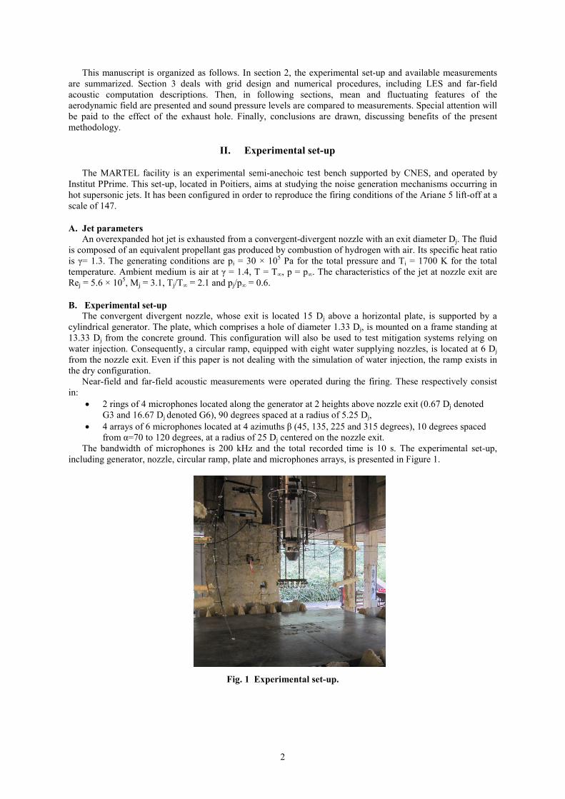
The bandwidth of microphones is 200 kHz and the total recorded time is 10 s. The experimental set-up, including generator, nozzle, circular ramp, plate and microphones arrays, is presented in Figure 1.

Fig. 1 Experimental set-up.

3

III. Numerical procedure

A. Computational tools The proposed methodology aims at fully coupling a Navier-Stokes solver to a full Euler acoustic solver in a

robust and precise way, in a demanding HPC context. To this purpose, ONERA in-house codes CEDRE [12] and SPACE [13] are respectively used and are fully coupled through the CWIPI library [14]. Both codes operate on unstructured grids which are needed to easily describe the complex geometries, typical of actual launch pads. The cut-off Strouhal is defined as:

Stc = (c∞ Dj)/(PPW dcell uj) PPW being the required number of point per wavelength and dcell the diameter of a mesh element. For instance, dcell is strictly equal to (√6/6)a in the case of a regular tetrahedron where a is its characteristic edge length.

1. LES The filtered compressible Navier-Stokes equations are solved with a Smagorinsky subgrid scale model with

a constant set to 0.18. The wall law is laminar, i.e. with friction equal to μu1/y1, subscript 1 standing for the center of the first wall cell. The computation takes into account two species in the gas phase: air and equivalent propellant gas, whose specific heats are respectively defined by a 7th order polynomial and a constant. The spatial scheme is second order, with an HLLC Riemann solver for flux calculation. The required discretization is PPW=20. Time integration is performed with a second order implicit Runge-Kutta scheme and the implicit linear system is solved with the GMRES algorithm including 15 sub-iterations.

2. CAA Euler propagation is carried out in a medium initially at rest (p∞, T∞, ρ∞=p∞/rT∞) and filled with air, whose

thermodynamic properties relies on a molecular weight and a specific heat ratio respectively set to 28.96 g/mol and 1.4. Time integration is performed with a second order explicit Runge-Kutta scheme. The spatial discretization relies on a discontinuous Galerkin method with Gauss-Lobatto quadratures. The spatial order is defined by p+1 where p is the degree of the polynomials. The use of 4thorder, i.e. p=3, is targeted in the propagation zone while decreasing this order in some areas, for robustness at the interface, for accuracy consistency in small cells at the rigid walls and for wave damping at the external boundaries. Such mapping will be detailed further ahead. The PPW for calculating Strouhal cut-off depends on the order: PPW=3 at 4th order and PPW=14 at 2nd order [16].

3. Coupling procedure The coupling is operated along a common boundary of the two solvers. In order to avoid temporal and

spatial aliasing, the solvers are set to operate at identical time steps and the coupling is conducted at every time step. Further, the boundary shares the same grid points on both sides, meaning that the grids are fully coincident along the coupling interface. The coupling is purely surfacic and no overlapping is needed, which greatly simplifies the coupling procedure in view of HPC computations. The order mapping allowed by the acoustic solver is used to match the solver order at the interface where the spatial resolution is dictated by the 2nd order LES simulation. Away from the interface, the grid in the acoustic domain is quickly coarsened, as the order of the acoustic solver is increased up to the 4th order, reducing the CPU cost while preserving the overall 2nd order accuracy of the simulation. These choices are essential in the proposed methodology and ensure a robust and consistent coupling, free of any aliasing problems, while keeping the accuracy and CPU costs under control. Another important point, allowed by the CWIPI library, is that no specific boundary condition is needed in any solver as the coupling interface can emulate existing boundary conditions of both solvers. The coupling procedure operates in a two-way mode, allowing the information to be freely exchanged from one solver to the other according to the physics of the solution. It has been thoroughly checked and validated thanks to a series of academic test cases [14].

B. Computational domain The cylindrical generator, including the nozzle, the perforated plate and the ground are included in a

cylindrical computational domain, whose radius is 33.33 Dj and total height is 61.75 Dj. The plate is 0.08 Dj thick. The cylindrical generator has a radius of 2 Dj, a height of 33.33 Dj and is width centered. As indicated before, the experimental set-up includes an annular ring equipped with eight water supplying nozzles and is then integrated in the computational domain.

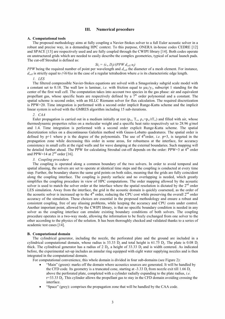
For computational convenience, this whole domain is divided in four sub-domains (see Figure 2): • “Main” (green): marks off the domain where acoustics sources are generated. It will be handled by

the CFD code. Its geometry is a truncated cone, starting at -3.33 Dj from nozzle exit till 1.66 Dj above the perforated plate, completed with a cylinder radially expanding to the plate radius, i.e. r=33.33 Dj. This cylinder allows the propellant gas to stay in the CFD domain avoiding crossing the interface.

• “Space” (grey): comprises the propagation zone that will be handled by the CAA code.

4

• “Below” (yellow): includes the area below the plate. It will be treated by the CFD code. • “Water_Nozzle” (blue, not visible on Figure 2): delimits the liquid part of injection nozzles. It is set

as inactive in this computation.

a. front view b. top view

Fig. 2 Computation domain and microphones.

As it can be seen on Figure 2, microphones located near the generator at 0.67 Dj in the “Main” domain are handled by the CFD code All others microphones are located in the “Space” domain, handled by the CAA code.

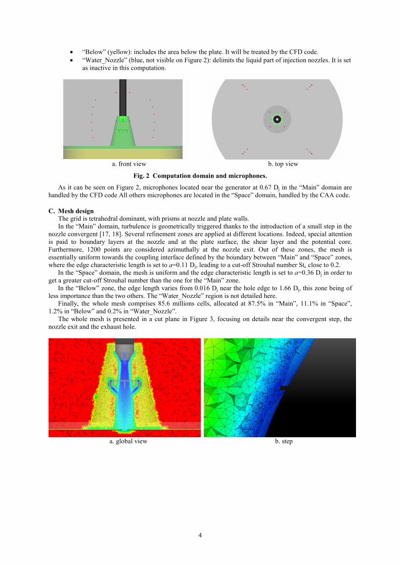
C. Mesh design The grid is tetrahedral dominant, with prisms at nozzle and plate walls. In the “Main” domain, turbulence is geometrically triggered thanks to the introduction of a small step in the

nozzle convergent [17, 18]. Several refinement zones are applied at different locations. Indeed, special attention is paid to boundary layers at the nozzle and at the plate surface, the shear layer and the potential core. Furthermore, 1200 points are considered azimuthally at the nozzle exit. Out of these zones, the mesh is essentially uniform towards the coupling interface defined by the boundary between “Main” and “Space” zones, where the edge characteristic length is set to a=0.11 Dj, leading to a cut-off Strouhal number Stc close to 0.2.

In the “Space” domain, the mesh is uniform and the edge characteristic length is set to a=0.36 Dj in order to get a greater cut-off Strouhal number than the one for the “Main” zone.

In the “Below” zone, the edge length varies from 0.016 Dj near the hole edge to 1.66 Dj, this zone being of less importance than the two others. The “Water_Nozzle” region is not detailed here.

Finally, the whole mesh comprises 85.6 millions cells, allocated at 87.5% in “Main”, 11.1% in “Space”, 1.2% in “Below” and 0.2% in “Water_Nozzle”.

The whole mesh is presented in a cut plane in Figure 3, focusing on details near the convergent step, the nozzle exit and the exhaust hole.

a. global view b. step

5

c. lips

d. exhaust hole

Fig. 3 Mesh edge length (arbitrary scale).

D. Order mapping As indicated in CAA description (cf. III.A.2), acoustic solver allows the use of order mapping. The default

order is set to 2nd. Several geometric boxes are spatially defined with the goal of imposing local orders. Interface with “Main” zone is matched with a 2nd order layer, transitioning to 4th order with an intermediate 3rd order layer. Lateral and top boundaries are set to 2nd order. Figure 4 allows the visualization of the spatial distribution of the polynomials degree in a cut plane. Finally, it must be noted that microphones located near the generator at 16.67 Dj are located in the default zone, set at 2nd order.

Fig. 4 Order mapping in “Space”.

E. Boundaries conditions The initial state consists in air at uniform conditions T∞, p∞. Regarding “Main” CFD zone, total quantities pi and Ti are prescribed at nozzle inlet, walls are adiabatic, and

the outlet is subsonic at p∞. Considering “Below” zone, same conditions as previous zone apply for the wall and the outlet.

In the CAA zone, walls are rigid and all outlets are subsonic non-reflective at p∞. “Main” and “Space” zones are coupled through a boundary denoted hereafter “Interface”. “Main” and

“Below” zones are linked through the “Hole” boundary.

F. Acoustic phase post-processing characteristics Characteristics of the acoustic computation are presented table 1. Setting a=0.11 Dj in the “Main” zone (except in nozzle) ensures that CFL = (c∞Δt)/dcell remains below 1 in

the jet near-field. All power spectral densities are directly calculated from numerical microphones with an in-house library. Computation has been performed on 1736 Intel cores, where 1512 cores were dedicated to CFD and 224 to CAA. This arbitrary proportion derives from the mesh distribution (89% vs. 11%, see paragraph III.C).

6

Table 1 Acoustic phase characteristics.

CPU time elapsed (h) 285 Total time computed (ms) 35

Total time computed (Dj/uj) ~1000 Time step Δt (s) 2.5 × 10-7

Samples 140 000 Acoustic sampling (Stac) 143

Number of averages 6 Frequency resolution (ΔSt) 3.6 × 10-3

IV. Aerodynamic near-field

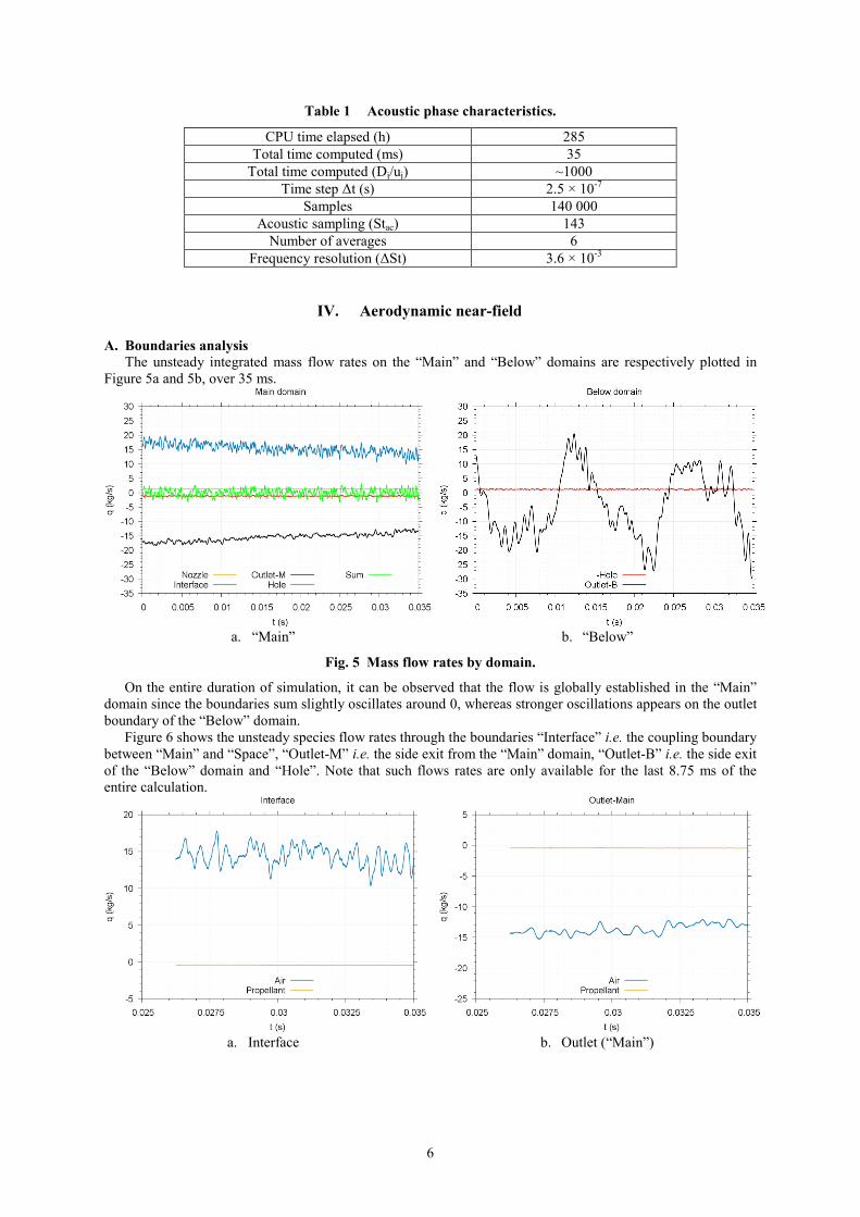
A. Boundaries analysis The unsteady integrated mass flow rates on the “Main” and “Below” domains are respectively plotted in

Figure 5a and 5b, over 35 ms.

a. “Main” b. “Below”

Fig. 5 Mass flow rates by domain.

On the entire duration of simulation, it can be observed that the flow is globally established in the “Main” domain since the boundaries sum slightly oscillates around 0, whereas stronger oscillations appears on the outlet boundary of the “Below” domain.

Figure 6 shows the unsteady species flow rates through the boundaries “Interface” i.e. the coupling boundary between “Main” and “Space”, “Outlet-M” i.e. the side exit from the “Main” domain, “Outlet-B” i.e. the side exit of the “Below” domain and “Hole”. Note that such flows rates are only available for the last 8.75 ms of the entire calculation.

a. Interface b. Outlet (“Main”)

7

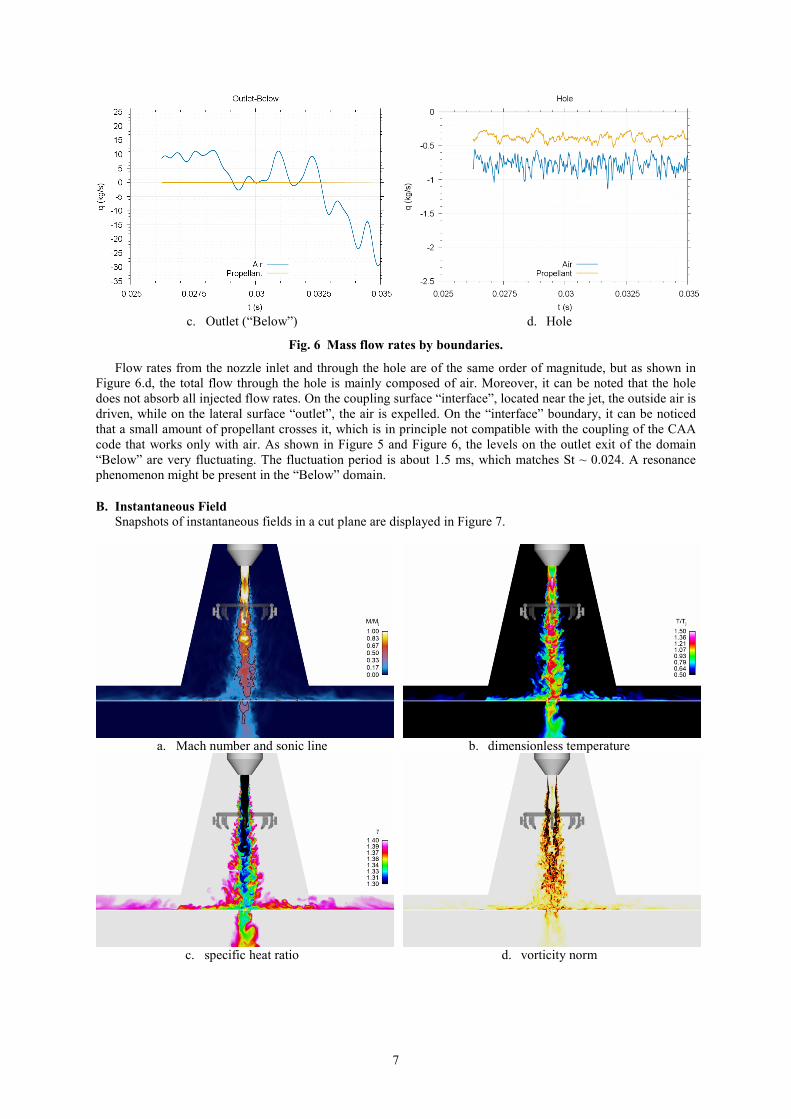
c. Outlet (“Below”) d. Hole

Fig. 6 Mass flow rates by boundaries.

Flow rates from the nozzle inlet and through the hole are of the same order of magnitude, but as shown in Figure 6.d, the total flow through the hole is mainly composed of air. Moreover, it can be noted that the hole does not absorb all injected flow rates. On the coupling surface “interface”, located near the jet, the outside air is driven, while on the lateral surface “outlet”, the air is expelled. On the “interface” boundary, it can be noticed that a small amount of propellant crosses it, which is in principle not compatible with the coupling of the CAA code that works only with air. As shown in Figure 5 and Figure 6, the levels on the outlet exit of the domain “Below” are very fluctuating. The fluctuation period is about 1.5 ms, which matches St ~ 0.024. A resonance phenomenon might be present in the “Below” domain.

B. Instantaneous Field Snapshots of instantaneous fields in a cut plane are displayed in Figure 7.

a. Mach number and sonic line b. dimensionless temperature

c. specific heat ratio d. vorticity norm

8

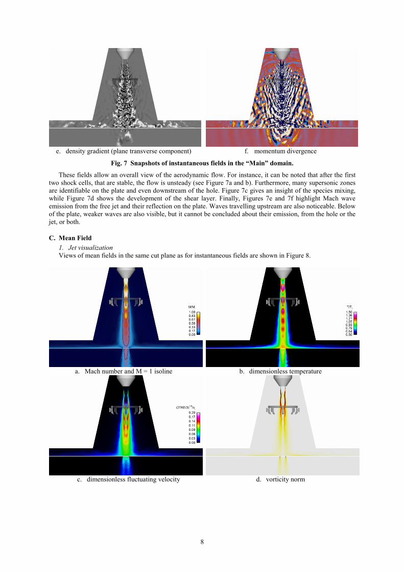
e. density gradient (plane transverse component) f. momentum divergence

Fig. 7 Snapshots of instantaneous fields in the “Main” domain.

These fields allow an overall view of the aerodynamic flow. For instance, it can be noted that after the first two shock cells, that are stable, the flow is unsteady (see Figure 7a and b). Furthermore, many supersonic zones are identifiable on the plate and even downstream of the hole. Figure 7c gives an insight of the species mixing, while Figure 7d shows the development of the shear layer. Finally, Figures 7e and 7f highlight Mach wave emission from the free jet and their reflection on the plate. Waves travelling upstream are also noticeable. Below of the plate, weaker waves are also visible, but it cannot be concluded about their emission, from the hole or the jet, or both.

C. Mean Field 1. Jet visualization Views of mean fields in the same cut plane as for instantaneous fields are shown in Figure 8.

a. Mach number and M = 1 isoline b. dimensionless temperature

c. dimensionless fluctuating velocity d. vorticity norm

9

e. dimensionless axial velocity and streamlines f. fluctuating pressure and velocity isolines

Fig. 8 Maps of mean fields in the “Main” domain.

These fields are averaged only on the last 12.25 ms (~350 Dj/uj) of the computation, due to informatics loss. The fact that the two first shock cells are quite stable is confirmed, as mean and instantaneous fields look the same in this region (see for instance Figure 8a and 8b). Sonic line allows the identification of two supersonic zones separated by the hole. Wall jet is detached in the hole vicinity, and then reattached on the plate (see Figure 8a and 8e). Strong velocity fluctuations (see Figure 8c) are produced after the first two shock cells, mainly at the shear layer location, before merging on the jet axis. Medium levels are maintained downstream in the mixing region, but also near the plate and after the hole (Figure 8.d). High vorticity levels are located at the hole edge. Figure 8e shows obviously high values of axial velocity along the jet axis that remains still high after the hole. The free jet induces a strong air entrainment which can be observed on streamlines, while contracting near the plate. Finally, Figure 8f draws isolines of ux/uj=1 in blue, ux/c∞=1 in cyan and a recall of M=1 line in black. The hole seems to induce a subsonic flow on the plate, unlike it could be expected without hole. Consequently, Mach wave emission of the deflected jet is not occurring. The fluctuating pressure shows high values in the jet and near the hole. High levels (over 160 dB) zones expand radially as height decreases. After the hole, the shape is radially constant. Far from the impingement region, levels near the plate reach lower values.

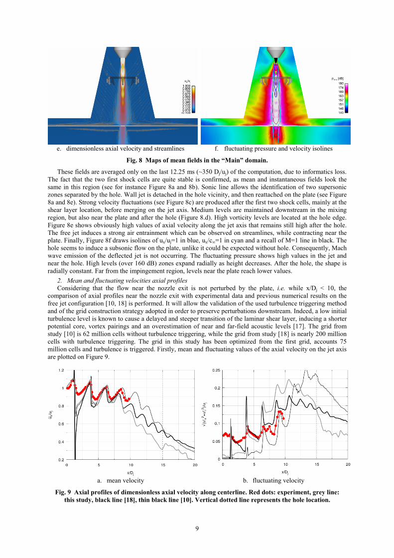
2. Mean and fluctuating velocities axial profiles Considering that the flow near the nozzle exit is not perturbed by the plate, i.e. while x/Dj < 10, the

comparison of axial profiles near the nozzle exit with experimental data and previous numerical results on the free jet configuration [10, 18] is performed. It will allow the validation of the used turbulence triggering method and of the grid construction strategy adopted in order to preserve perturbations downstream. Indeed, a low initial turbulence level is known to cause a delayed and steeper transition of the laminar shear layer, inducing a shorter potential core, vortex pairings and an overestimation of near and far-field acoustic levels [17]. The grid from study [10] is 62 million cells without turbulence triggering, while the grid from study [18] is nearly 200 million cells with turbulence triggering. The grid in this study has been optimized from the first grid, accounts 75 million cells and turbulence is triggered. Firstly, mean and fluctuating values of the axial velocity on the jet axis are plotted on Figure 9.

a. mean velocity b. fluctuating velocity

Fig. 9 Axial profiles of dimensionless axial velocity along centerline. Red dots: experiment, grey line: this study, black line [18], thin black line [10]. Vertical dotted line represents the hole location.

10

First of all, regarding the mean velocity, the location of the first two shock cells is well predicted by the computation, even if their intensities are over-estimated. Third shock location and intensity are well recovered by the computation, in contrary of the fourth one. Until the third shock cell, all computations show similarity results, but thereafter, the velocity decay has different profiles. Secondly, when looking at fluctuating velocity, it can be noticed that even if levels are small at the nozzle exit, computations including a small step in the nozzle exhibit stronger levels, particularly downstream of the second shock cell. After the third shock cell, discrepancies appear, levels being nearly 1.5 higher from one computation to another. Nevertheless, effects of the geometrical triggering seem beneficial for the prediction of velocity fluctuations.

3. Mean and fluctuating velocities radial profiles LDV measurements provide radial profiles of mean and fluctuating velocities at four axial positions.

Comparison of experimental and numerical values are plotted Figure 10. In order to estimate quantities at the nozzle exit, numerical radial profiles at this location are also provided.

a. axial mean velocity b. axial fluctuating velocity

c. radial mean velocity d. radial fluctuating velocity

Fig. 10 Radial profiles of axial and radial, mean and fluctuating velocity (normalized by uj) at four axial locations as a function of r/Dj. Red dots: experiment, grey line: this study, black line [18],

thin black line [10].

At nozzle exit, the improvement due to the turbulence tripping is clear on fluctuating velocities that present non-null levels. Otherwise, mean velocity levels are unchanged, but maximum is obtained at lower r/Dj, indicating a less thick shear layer. When going further downstream, it can be noted that at x=1 Dj and 3.7 Dj, mainly radial velocity does not exhibit the experimental shape of profiles. It must be emphasized that axial positions x/Dj=1 and 3.7 are located in the vicinity of shock cells as seen on Figure 9. Generally, turbulence trigging is beneficial to recover high levels of fluctuations, but as small discrepancies come out from computations taking into account such mechanism, it is thought to be explained by grid sensitivity. Therefore, additional work has to be done in order to tradeoff between precision and cost.

Finally, two radial quantities are defined: the half-radius r0.5, radius where ux = 0.5 ux0, and the shear layer thickness δ, distance between the radius where ux = 0.1 ux0 and the radius where ux = 0.9 ux0, where ux0 is the value of ux on the axis in a given section. These two quantities are plotted in Figure 11.

11

Fig. 11 Axial evolution of half-radius and shear layer thickness.

The end of the potential core is determined by the position where δ = 2r0.5, that is to say where the two curves merge. On the plot, this location is near the hole at 14.5 Dj, where the flow is strongly disrupted. Thus, a reasonable location for the end of potential core may be where the two curves become parallel, which is near 8.75 Dj.

4. Mean profiles on the interface As said previously, the coupling interface is composed of a conical part near the jet axis and of a cylindrical

part above the plate. Values of fluctuating pressure are plotted along the intersection of the interface with a vertical plane. Figure 12a displays its radial evolution. The left dotted line indicates the location of the top of the truncated cone and the right one the location of the bottom of the truncated cone. Figure 12b displays its axial evolution.

a. radial evolution b. axial evolution

Fig. 12 Fluctuating pressure on the coupling surface.

Levels on the interface upstream of the nozzle exit are almost constant (nearly 150 dB). Downstream of the nozzle exit, levels are increasing to nearly 165 dB at the cone bottom. Then, the levels decrease as the distance from the axis increases. Such high levels consolidate the non-linear assumption and thus the use of an Euler solver rather than a linear integral method.

5. Mean profiles on the plate Finally, Figure 13 presents remarkable quantities along the intersection of the plate with a vertical plane.

First, the instantaneous value of y+ is plotted on Figure 13a. Levels are mainly around 30, which is a little too high in order to finely catch all features of the flow. Profile of wall friction in Figure 13b shows that a maximum is obtained at few diameters from the exhaust hole, probably indicating that the jet width is too large to entirely fit in the hole. Figure 13c indicates that jet temperature is maximum at the hole edge, before cooling down away from it. At last, fluctuating pressure levels behave in the same way as temperature and do not seem correlated with friction (see Figure 13d). It could be noted that fluctuating pressure is nearly 190 dB near the hole, this location being the highest value in the whole “Main” domain (except at shocks locations). These levels are of the same order of those on the interface (Figure 12a, reported on Figure 13d in thin black line) from r/Dj ~7.5 to ~9, and till r/Dj=33, levels on the interface are higher than levels on the plate with a maximum reaching 7.5 dB

12

near r/Dj~14, and an inversion between r/Dj=22 and 24, mainly due to the bump at this location on the plate. Otherwise, difference is about 2 dB.

a. dimensionless wall distance b. friction

c. dimensionless temperature d. fluctuating pressure (thin line: interface values)

Fig. 13 Radial evolution of characteristics quantities on the plate.

V. Acoustic near and far-field

A. Instantaneous field Figure 14 displays instantaneous maps of pressure field and momentum norm in a cut plane, allowing

appreciating the continuity of the acoustic solution at the crossing of the CFD-CAA interface.

a. pressure field a. momentum norm field

Fig. 14 Snapshots of instantaneous near and far-fields.

13

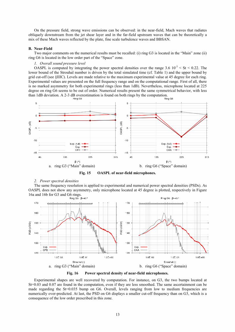
On the pressure field, strong wave emissions can be observed: in the near-field, Mach waves that radiates obliquely downstream from the jet shear layer and in the far-field upstream waves that can be theoretically a mix of these Mach waves reflected by the plate, fine scale turbulence waves and BBSAN.

B. Near-Field Two major comments on the numerical results must be recalled: (i) ring G3 is located in the “Main” zone (ii)

ring G6 is located in the low order part of the “Space” zone. 1. Overall sound pressure level OASPL is computed by integrating the power spectral densities over the range 3.6 10-3 < St < 0.22. The

lower bound of the Strouhal number is driven by the total simulated time (cf. Table 1) and the upper bound by grid cut-off (see §IIIC). Levels are made relative to the maximum experimental value at 45 degree for each ring. Experimental values are presented on the full frequency range and on the computational range. First of all, there is no marked asymmetry for both experimental rings (less than 1dB). Nevertheless, microphone located at 225 degree on ring G6 seems to be out of order. Numerical results present the same symmetrical behavior, with less than 1dB deviation. A 2-3 dB overestimation is found on both rings by the computation.

a. ring G3 (“Main” domain) b. ring G6 (“Space” domain)

Fig. 15 OASPL of near-field microphones.

2. Power spectral densities The same frequency resolution is applied to experimental and numerical power spectral densities (PSDs). As

OASPL does not show any asymmetry, only microphone located at 45 degree is plotted, respectively in Figure 16a and 16b for G3 and G6 rings.

a. ring G3 (“Main” domain) b. ring G6 (“Space” domain)

Fig. 16 Power spectral density of near-field microphones.

Experimental shapes are well recovered by computation. For instance, on G3, the two bumps located at St=0.03 and 0.07 are found in the computation, even if they are less smoothed. The same ascertainment can be made regarding the St=0.035 bump on G6. Overall, levels ranging from low to medium frequencies are numerically over-predicted. At last, the PSD on G6 displays a smaller cut-off frequency than on G3, which is a consequence of the low order prescribed in this zone.

14

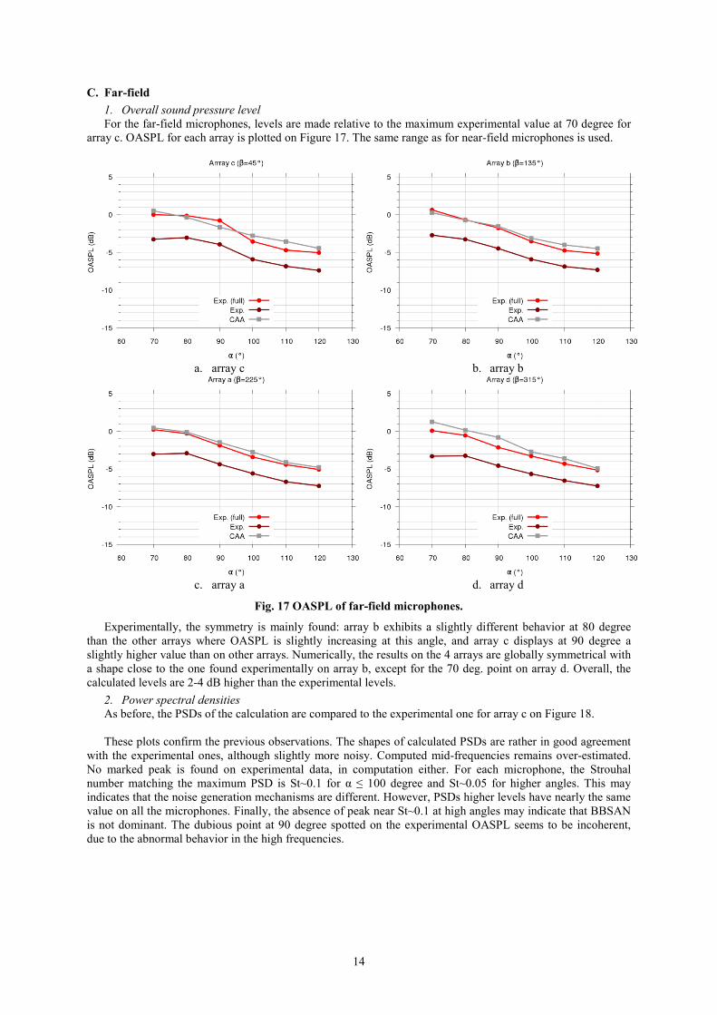
C. Far-field 1. Overall sound pressure level For the far-field microphones, levels are made relative to the maximum experimental value at 70 degree for

array c. OASPL for each array is plotted on Figure 17. The same range as for near-field microphones is used.

a. array c b. array b

c. array a d. array d

Fig. 17 OASPL of far-field microphones.

Experimentally, the symmetry is mainly found: array b exhibits a slightly different behavior at 80 degree than the other arrays where OASPL is slightly increasing at this angle, and array c displays at 90 degree a slightly higher value than on other arrays. Numerically, the results on the 4 arrays are globally symmetrical with a shape close to the one found experimentally on array b, except for the 70 deg. point on array d. Overall, the calculated levels are 2-4 dB higher than the experimental levels.

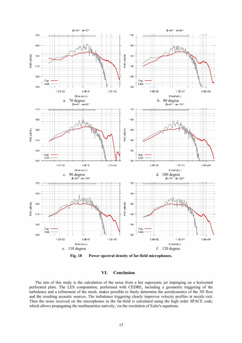
2. Power spectral densities As before, the PSDs of the calculation are compared to the experimental one for array c on Figure 18. These plots confirm the previous observations. The shapes of calculated PSDs are rather in good agreement

with the experimental ones, although slightly more noisy. Computed mid-frequencies remains over-estimated. No marked peak is found on experimental data, in computation either. For each microphone, the Strouhal number matching the maximum PSD is St~0.1 for α ≤ 100 degree and St~0.05 for higher angles. This may indicates that the noise generation mechanisms are different. However, PSDs higher levels have nearly the same value on all the microphones. Finally, the absence of peak near St~0.1 at high angles may indicate that BBSAN is not dominant. The dubious point at 90 degree spotted on the experimental OASPL seems to be incoherent, due to the abnormal behavior in the high frequencies.

15

a. 70 degree b. 80 degree

c. 90 degree d. 100 degree

e. 110 degree f. 120 degree

Fig. 18 Power spectral density of far-field microphones.

VI. Conclusion

The aim of this study is the calculation of the noise from a hot supersonic jet impinging on a horizontal perforated plate. The LES computation, performed with CEDRE, including a geometric triggering of the turbulence and a refinement of the mesh, makes possible to finely determine the aerodynamics of the 3D flow and the resulting acoustic sources. The turbulence triggering clearly improves velocity profiles at nozzle exit. Then the noise received on the microphones in the far-field is calculated using the high order SPACE code, which allows propagating the nonlinearities natively, via the resolution of Euler's equations.

16

Regarding this calculation, the first point to emphasize is the position of the coupling interface between the CFD domain and the CAA domain. Indeed, the propellant jet results of combustion products and since the CAA code only works with air, the interface must not be positioned in a region where there are products other than air. This positioning is all the more delicate as the presence of the plate induces possible recirculations of the species. The calculation presents a satisfactory establishment in terms of flow balancing in the “Main” domain. Moreover, it can be noted that the flow under the plate is totally unsteady, and that resonance phenomena can appear. Besides, the jet becomes subsonic just upstream of the hole and returns to supersonic downstream of it. The jet flow along the plate is subsonic. Even if a brief analysis of the near-wall flow shows a high fluctuating pressure level in the vicinity of the exhaust hole, the acoustic emission of the hole remains to be investigated. A parametric study of the hole width (providing a link between the jet shear layer growth and its propensity to spill out the exhaust hole) may help to characterize it.

From the point of view of far-field acoustics, the experimental shape of the OASPLs curves or of PSDs is well recovered by the simulation. However, the calculated levels are higher than the experimental levels, 2-4 dB on the far-field arrays, and 2-3 dB on the near-field antennas, mainly in medium frequencies. The overestimation can come from the reflection of Mach waves, which is thought to be the dominant noise component on the plate. A better description of the wall boundary layer is therefore needed. For this purpose, a surface refinement of the plate, combined with an adequate model (wall law or RANS -ZDES- treatment) is envisaged. It is not currently possible to specify precisely the influence of the plate on the far-field radiated noise. Additional experimental microphones at lower angles could also help understanding involved acoustic phenomena.

The next step is to perform a computation following the same CFD-CAA procedure activating water supplying nozzles as noise mitigation devices.

Acknowledgments This study is supported by the French national space agency CNES and ONERA scientific direction.

Authors are grateful to G. Chaineray and E. Quémerais for their work on coupling capabilities and C. Peyret for his advices on the use of SPACE.

References [1] Brès, G. A., Jaunet, V., Le Rallic, M., Jordan, P., Colonius, T., and Lele, S.K. “Large eddy simulation for jet noise: the

importance of getting the boundary layer right”. In 21st Aeroacoustics Conference, Dallas, TX, 2015. AIAA/CEAS. 2015-2535.

[2] Bogey, C., Marsden, O., and Bailly, C. “Influence of initial turbulence level on the flow and sound fields of a subsonic jet at a diameter-based Reynolds number of 105”. J. Fluid Mech., 701:352–385, 2012.

[3] de Cacqueray, N., Bogey, C., and Bailly, C. “Investigation of a High-Mach-Number Overexpanded Jet Using Large-Eddy Simulation”. AIAA Journal, 49(10):2171–2182, 2011

[4] Tsutsumi, S. and Terashima, K. “Validation and Verification of a Numerical Prediction Method for Lift-off Acoustics of Launch Vehicles”. Trans. JSASS Aerospace Tech. Japan, 15:7–12, 2017.

[5] Brehm, C., Housman, J, and Kiris, C. “Noise generation mechanisms for a supersonic jet impinging on an inclined plate”. J. Fluid Mech., 797:802–850, 2016.

[6] Akamine, M., Okamoto, K, Gee, K.L., Neilsen, T.B., Teramoto, S., Okunuki, T., and Tsutsumi, S. “Effect of Nozzle Plate Distance on Acoustic Phenomena from Supersonic Impinging Jet”. AIAA Journal, 56(5):1943– 1952, 2018.

[7] Dauptain, A., Gicquel, L. Y. M. and Moreau, S. “Large Eddy Simulation of Supersonic Impinging Jets”. AIAA Journal, 50(7):1560–1574, 2012.

[8] Tsutsumi, S., Takaki, R., Ikaida, H., and Terashima, K. “Numerical Aeroacoustics Analysis of a Scaled Solid Jet Impinging on Flat Plate with Exhaust Hole”. In 30th International Symposium on Space Technology and Science, Kobe, Japan, 2015. 2015-o-2-05

[9] Kawai, S., Tsutsumi, S., Takaki, R., and Fujii, K. “Computational Aeroacoustic Analysis of Overexpanded Supersonic Jet Impingement on a Flat Plate with/without Hole”. In 5th Fluids Engineering Conference, San Diego, CA, 2007. ASME/JSME. FEDSM2007-37563.

[10] Langenais, A., Vuillot, F., Troyes, J., and Bailly, C. “Numerical investigation of the noise generated by a rocket engine at lift-off conditions using a two-way coupled CFD-CAA method”. In 23rd Aeroacoustics Conference, Denver, CO, 2017. AIAA/CEAS. 2017-3212.

[11] Gély, D., Valière, J.-C., Lambaré, H. and Foulon, H. “Overview of aeroacoustic research activities in MARTEL facility applied to jet noise”. In 35th International Congress and Exposition on Noise Control Engineering, Honolulu, HW, 2006

[12] A. Refloch, B. Courbet, A. Murrone, P. Villedieu, C. Laurent, P. Gilbank, J. Troyes, L. Tessé, G. Chaineray, J.-B. Dargaud, E. Quémerais, and F. Vuillot. “CEDRE Software”. Aerospace Lab, (2), 2011.

[13] Léger, R., Peyret, C., and Piperno, S. “Coupled Discontinuous Galerkin/Finite Difference Solver on Hybrid Meshes for Computational Aeroacoustics”. AIAA Journal, 50(2):338–349, 2012.

[14] Quémerais E., “Coupling with interpolation parallel interface”. 2016, https://w3.onera.fr/cwipi/ [15] Delorme, P., Mazet, P., Peyret, C., and Ventribout, Y. “Computational aeroacoustics applications based on a

discontinuous Galerkin method”. C. R. Mécanique, 333:676–682, 2005.

17

[16] Langenais, A., Vuillot, F., Peyret, C., Chaineray, G., and Bailly, C. “Assessment of a Two-Way Coupling Methodology Between a Flow and a High-Order Nonlinear Acoustic Unstructured Solvers”. Flow Turbulence Combust, 2018

[17] Lorteau M., Cléro F., and Vuillot F., “Analysis of noise radiation mechanisms in hot subsonic jet from a validated large eddy simulation solution”. Physics of Fluids 27, 075108, 2015

[18] Langenais A., Vuillot F., Troyes J., and Bailly C., “Accurate simulation of the noise generated by a hot supersonic jet including turbulence tripping and nonlinear acoustic propagation”. Physics of Fluids 31, 016105, 2019