Embed Size (px)
Citation preview

County-level climate change information to supportdecision-making on working lands
Emile Elias1 & T. Scott Schrader1 & John T. Abatzoglou2 &
Darren James1 & Mike Crimmins3 & Jeremy Weiss4 &
Albert Rango1
Received: 28 April 2016 /Accepted: 17 July 2017 /Published online: 28 August 2017# The Author(s) 2017. This article is an open access publication
Abstract Farmers, ranchers, and forest landowners across the USA make weather- andclimate-related management decisions at varying temporal and spatial scales, often with inputfrom local experts like crop consultants and cooperative extension (CE) personnel. In order toprovide additional guidance to such longer-term planning efforts, we developed a tool that
Climatic Change (2018) 148:355–369DOI 10.1007/s10584-017-2040-y
This article is part of a Special Issue on ‘Vulnerability of Regional Forest and Agricultural Ecosystems to aChanging Climate (USDA Southwest Climate Hub)’ edited by David Gutzler and Connie Maxwell
Electronic supplementary material The online version of this article (doi:10.1007/s10584-017-2040-y)contains supplementary material, which is available to authorized users.
* Emile [email protected]
T. Scott [email protected]
John T. [email protected]
Darren [email protected]
Mike [email protected]
Jeremy [email protected]
Albert [email protected]
1 U.S. Department of Agriculture–Agricultural Research Service, Jornada Experimental Range, LasCruces, NM, USA
2 Department of Geography, University of Idaho, Moscow, ID 83844, USA3 Department of Soil, Water and Environmental Science, University of Arizona, Tucson, AZ 85721,
USA4 School of Natural Resources and the Environment, University of Arizona, Tucson, AZ 85721, USA

shows statistically downscaled climate projections of temperature and precipitation consoli-dated to the county level for the contiguous US. Using the county as a fundamental mappingunit encourages the use of this information within existing institutional structures like CE andother U.S. Department of Agriculture (USDA) programs. A Bquick-look^ metric based on thespatial variability of climate within each county aids in the interpretation of county-levelinformation. For instance, relatively higher spatial variability within a county indicates thatmore localized information should be used to support stakeholder planning. Changes in annualprecipitation show a latitudinal dipole where increases are projected for much of the northernUS while declines are projected for counties across the southern US. Seasonal shifts in county-level precipitation are projected nationwide with declines most evident in summer months inmost regions. Changes in the spatial variability of annual precipitation for most counties wereless than 10 mm, indicating fairly spatially homogenous midcentury precipitation changes atthe county level. Annual and seasonal midcentury temperatures are projected to increase acrossthe USA, with relatively low change in the spatial variability (<0.3 °C) of temperature acrossmost counties. The utility of these data is shown for forage and almond applications, bothindicating a potential decline in production in some future years, to illustrate use of county-level seasonal projections in adaptation planning and decision-making.
Keywords Climate change . Decision-making . Agriculture . Forestry . Ranching . USDAclimate hubs . Cooperative extension
1 Introduction
Impacts of climate change on agriculture include redistribution of water availability, changes inthe thermal suitability for agricultural zones, and changes in erosion and crop productivity.Adaptation planning, such as considering alternate crops and management strategies, andconservation practices for nutrients, soil, and water resources can minimize the impacts ofclimate variability and change on the agricultural sector (Walthall et al. 2012). In general, cropproductivity may decline in response to increases in temperature, but impacts vary among croptype and region (Walthall et al. 2012).
Farmers and ranchers frequently make decisions based upon changing weather conditionsand longer-term climate projections may be helpful to sectoral planning. Rising temperaturesare projected to have far-reaching impacts on the agricultural sector in the USA (Schaubergeret al. 2017), especially in combination with decreased water availability (Anderson et al.2015). The increased frequency, duration, and intensity of drought and heat waves mayexacerbate livestock and crop stress, resulting in greater susceptibility to disease and peststhat may have increased occurrences, higher intensities, and expanded ranges (Anyamba et al.2014; Deryng et al. 2014; Walthall et al. 2012). Agriculturists cope within an expected range ofconditions relative to their locations; however, increased temperatures will alter growingseasons with earlier starts and longer duration, more high-temperature days, and warmerwinters with fewer nights below freezing. These climatic changes can produce both negativeand positive effects, for example while warmer winters may reduce yields of chill-dependedcrops (Luedeling et al. 2009), they can also lengthen the growing season of other crops andexpand the potential range of agricultural crops currently limited by short growing seasons orinsufficient heat accumulation. Increasing atmospheric carbon dioxide (CO2) can boost plantgrowth, thus in some regions, climate change could lead to enhanced productivity, especially
356 Climatic Change (2018) 148:355–369
in areas with limited precipitation. However, elevated CO2 can also disproportionately stim-ulate the growth of weed species that can also reduce grain and forage quality (Walthall et al.2012). Impacts to the US agricultural sector are dependent upon actions taken to supportregional and local adaptive management.
1.1 USDA Regional Climate Hubs
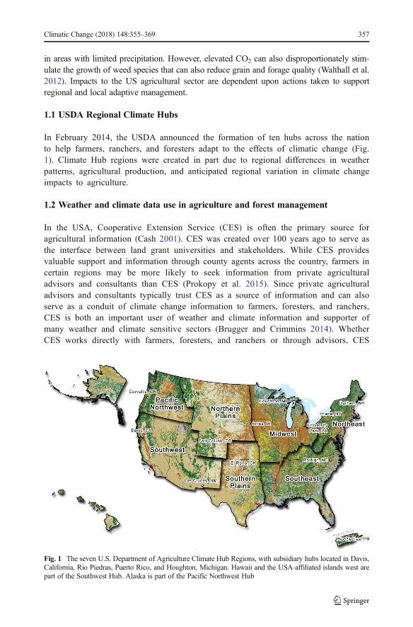
In February 2014, the USDA announced the formation of ten hubs across the nationto help farmers, ranchers, and foresters adapt to the effects of climatic change (Fig.1). Climate Hub regions were created in part due to regional differences in weatherpatterns, agricultural production, and anticipated regional variation in climate changeimpacts to agriculture.
1.2 Weather and climate data use in agriculture and forest management
In the USA, Cooperative Extension Service (CES) is often the primary source foragricultural information (Cash 2001). CES was created over 100 years ago to serve asthe interface between land grant universities and stakeholders. While CES providesvaluable support and information through county agents across the country, farmers incertain regions may be more likely to seek information from private agriculturaladvisors and consultants than CES (Prokopy et al. 2015). Since private agriculturaladvisors and consultants typically trust CES as a source of information and can alsoserve as a conduit of climate change information to farmers, foresters, and ranchers,CES is both an important user of weather and climate information and supporter ofmany weather and climate sensitive sectors (Brugger and Crimmins 2014). WhetherCES works directly with farmers, foresters, and ranchers or through advisors, CES
Fig. 1 The seven U.S. Department of Agriculture Climate Hub Regions, with subsidiary hubs located in Davis,California, Rio Piedras, Puerto Rico, and Houghton, Michigan. Hawaii and the USA-affiliated islands west arepart of the Southwest Hub. Alaska is part of the Pacific Northwest Hub
Climatic Change (2018) 148:355–369 357

requires reputable weather and climate data for customers. The required data, howev-er, depends upon the intended management actions as decisions are made withdifferent time horizons. For example, foresters selecting trees adapted to midcenturytemperatures require different information than farmers who are currently growingannual crops, or considering planting fruit or nut trees that might reach maturation inthe next decade.
Incorporating weather information in agricultural management and planning has beenshown to improve economic returns (Fuglie et al. 2007; Lazo et al. 2011; Solís and Letson2013). On longer-term horizons, adaptive responses to climate change such as the selection ofviable cropping systems would benefit from accessible temperature and precipitation informa-tion. Similarly, adaptive and informed forest management, such as assisted migration, will helpbuild resilience in private and public forests (Duveneck and Scheller 2015; Williams andDumroese 2013).
The impact of climate on crop yield prompted some of the first instrumented temperaturemeasurements in the USA in 1731–1732 in Philadelphia (Fiebrich 2009). Today, weather ismeasured by a variety of networks and systems integrate data from over 10,000 stations,including volunteer observer networks, across the USA (Fiebrich 2009). These observationsprovide the foundation for understanding spatiotemporal variability of weather and climate,and are the primary basis for assessing climate variability and change. However, the observa-tional climate network can suffer from inadequate station density, lack of long-term andcontinuous observations and quality control issues (Abatzoglou 2013; Menne et al. 2012).Gridded surface meteorological data have been developed by incorporating these observationswith a variety of other considerations (e.g., topography, proximity to water) to provide spatiallyand temporally complete estimates (Abatzoglou 2013; Daly et al. 2008).
1.3 Data to support county-level decision-making
Support for agricultural decision-making is typically organized along political bound-aries in the USA. Many counties have USDA service centers, housing the NaturalResources Conservation Service, the Farm Service Agency, Rural Development, andoften county CES agents. Since counties are the typical organizational unit whereinformation is sought and county agents have expressed the need for more long-termdata, we developed a county-level dataset of projected midcentury temperature andprecipitation for adaptation planning.
2 Methods
2.1 Datasets
2.1.1 Historical climate data
We used the 30-year normals data (1971–2000) from the PRISM Climate Group to representhistorical temperature and precipitation (Daly et al. 2008). This is a baseline dataset describingaverage seasonal and annual maximum temperature (Tmax; °C), minimum temperature (Tmin;°C), and total precipitation (ppt; mm). The normals dataset covers the contiguous US at an800-m (1/120th degree) spatial resolution.
358 Climatic Change (2018) 148:355–369

2.1.2 Climate projection data
We used statistically downscaled climate projections from 20 general circulation models(GCM) participating in the Coupled Model Inter-comparison Project 5 (CMIP5). The Multi-variate Adaptive Constructed Analogs (MACA) downscaling approach (Abatzoglou 2013)was used as it has been shown to be able to better capture details of spatiotemporal variabilityin climate across the mountainous western US.
We specifically focus on midcentury (2040–2069) projections for the contiguous US usingclimate experiments run with forcing from Representative Concentration Pathway 8.5 (RCP8.5). MACA downscales daily GCM fields of Tmax, Tmin, and ppt (among other variables),using a linear combination of historical spatial analogs for mapping GCM fields and anequidistant quantile mapping bias correction (Li et al. 2010; Pierce et al. 2015). Wedownloaded the MACAv2-METDATA monthly multi-model mean from 20 models of expect-ed change between 1971 and 2000, representing historic PRISM and MACA, and 2040–2069 at the 4000-m (1/24th degree) resolution.
2.1.3 Historic data spatial resolution
Both the 30-year 1971–2000 normals from PRISM (800 m) and MACA (4000 m) wereconsidered to represent the historic condition. While the MACA data used a dataset that usedPRISM time series data, they were produced at a coarser spatial resolution and correspond tomodel years (1971–2000) that may differ from observed normals slightly due to internalclimate variability. We analyzed the difference in 1971–2000 annual and seasonal climatenormals from the PRISM and MACA datasets (Online resource (OR) I). County-level historicdata were strongly correlated (R2 = 0.971 to 0.9995) despite the difference in originalspatial resolution and internal climate variability. There were only nominal differencesin county-level Tmax, Tmin, and precipitation (mean bias, Tmax 0.2 °C, Tmin 0.3 °C,precipitation −1.1%). This similarity was expected as both datasets use the same basedata (PRISM) and the aggregation of these data to the county level largely negates anydifferences. Given the historic normal data similarity between PRISM and MACA, andthe end-user familiarity with PRISM, we opted to use PRISM data as the normalbackground condition.
2.2 Data processing and analysis
To generate a historical baseline dataset, we used PRISM data to calculate a county-level mean and standard deviation using ArcGIS and zonal statistics for seasonal andannual Tmax, Tmin, and ppt to represent Bnormal^ historic conditions. Seasons weredefined as winter (December-January-February), spring (March-April-May), summer(June-July-August), and fall (September-October-November). Next, we generated asecond dataset (MACA) to represent the projected change for each county betweenthe 2040–2069 and 1971–2000 time periods by using ArcGIS and zonal statistics torepresent the change from historic conditions. Thus, means for historic conditions andfuture changes at the county level were developed discretely. We then summed theseasonal and annual average values from the corresponding multi-model mean tocalculate the future values for each county. This approach of using downscaled datato estimate future change and apply the anticipated change to an alternate baseline
Climatic Change (2018) 148:355–369 359

dataset has precedent (Sofaer et al. 2017). We additionally calculated the standarddeviation (SD) of mean changes among all 4-km pixels within each county, or the SDof the change data layer.
SD can be used as an estimate of the variability in the expected changes in Tmax, Tmin,and ppt across a county. SD represents the amount of variation in the pixel values comprising acounty and is derived from the projected changes in Tmax, Tmin, and ppt, not future valueprojections, which are the sum of historic and projected change values. SD is used to evaluatethe spatial variation in change. SD values closer to zero indicate a more spatially homogenousrange of projected values and higher SD indicates more variability within the projected change.Users can use SD to decide if the average change in county values is sufficient to answer aspecific question for their location, or if more spatially detailed information is warranted.
Results presented as average shifts in seasonal and annual conditions provide anestimate of future changes for scenario planning. However, we present only changesin mean climate distilled from 20 different GCM projections. This has advantages forsome consumers as it avoids introducing the concepts of ensembles and uncertainties.In addition, the multi-model mean is often superior to any single model (Tebaldi andKnutti 2007). However, the full spread of projected changes in climate may be usefulfor more sophisticated consumers of information, particularly those which might wantto devise adaptation strategies for a range of climate projections. Additionally, 30-yearclimatological summaries may help support dialog and planning, but may not suffi-ciently incorporate climatic extremes for scenario planning.
3 Results and discussion
3.1 National county-level dataset summary
National and regional maps and data are available as online resources supplemental to thisarticle and at http://swclimatehub.info/data.
3.1.1 Precipitation
For most of the northern US, total precipitation is projected to increase and shift seasonally(OR II and III). Conversely, total precipitation is projected to decline across parts of thesouthern US. Declines in precipitation are most evident during the summer months acrossthe nation.
In 92% of counties of the nation, the annual precipitation SD was less than 10 mm,indicating that the change in midcentury precipitation varies by less than 10 mm across eachcounty (OR IV). Counties with annual and seasonal precipitation SD larger than 10 mm weregenerally located in mountainous regions of the USA, particularly the Rocky Mountain andAppalachian regions. Nearly all eastern US counties had annual and seasonal precipitation SDless than 10 mm. Based upon SD, seasonal and annual precipitation change for each countyappears fairly homogenous for most of the USA suggesting projected changes in countyprecipitation values from the dataset could likely adequately represent mean county-levelchanges in most parts of the country. Projections of precipitation change in some counties ofthe Northwest, Northern Plains and Southwest Regions should be evaluated prior to applyingchanges uniformly across the counties.
360 Climatic Change (2018) 148:355–369

3.1.2 Temperature
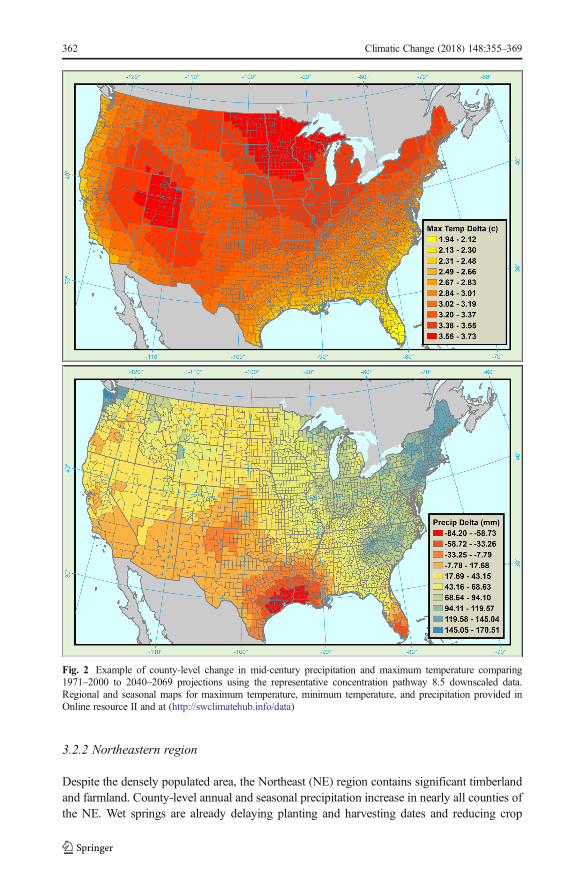
Nationally, annual and seasonal mid-century Tmax (Fig. 2) and Tmin increase in all counties.The magnitude of the increase varies slightly by region and season. Annual Tmax increases areslightly higher for the Midwest and Northern Plains regions, and slightly lower in theSoutheast region, with all regional increases ranging from 2.4 to 3.9 °C. Southeast, SouthernPlains, and Southwest county summer median Tmax is near or higher than the thermaltolerance for some crops in certain counties (Hatfield et al. 2011; Luck et al. 2011). IncreasedTmax in these regions may further limit production of certain crops. Future winter Tmin willincrease most in the coldest counties (+5 °C) and less for warmer counties (+2 °C). Increases inwinter Tmin can adversely impact perennial crops with winter chilling requirements(Baldocchi and Wong 2008; Lobell and Field 2011) and snowpack accumulation. Conversely,warming of winter Tmin may allow for expansion of cold intolerant perennials (Parker andAbatzoglou 2016). Mean annual and seasonal anticipated changes provide a platformfor evaluating and planning for both positive and negative potential impacts on specificcommodities and ecosystems.
Tmax SD is less than 0.3 °C for all counties of the nation, indicating that the projectedchange in mean Tmax across counties is fairly spatially homogeneous. Most eastern countieshave a lower annual and seasonal Tmax SD. The larger western counties located along thePacific Coast have a wider ranging Tmax SD, with the largest Tmax SD occurring in summer.Tmin SD is also typically less than 0.3 °C. Most eastern counties have a low annual andseasonal Tmin SD, with the exception of some larger counties in Maine in winter. Winter TminSD was largest for some inland western counties whereas summer Tmin SD was largest forcounties along the Pacific Coast. Given the low Tmax and Tmin SD (<0.3 °C) for mean annualand seasonal temperature changes in each county of the nation, compared to the daily variationin temperature at one location, the projected mean changes in temperature can be readilyapplied to counties nationwide. Data tables can be used (OR II) to estimate the 95% range ofpixels comprising county values as the mean ± 2SD.
3.2 Regional summaries
3.2.1 Midwestern region
In the Midwest (MW), corn and soybean production occur on 75% of the arable land.Precipitation is projected to increase in fall, winter, and spring and decrease in summer. Theincrease in spring precipitation may reduce the number of workable field days and disruptplanting operations in the region (Hatfield et al. 2015). The median annual increase in countyprecipitation in the MW is projected to be 64 mm, mostly occurring in the winter and spring.The maximum annual ppt change SD of all the counties in the MW is 15.2 mm, suggestingrelatively homogenous county-level precipitation change.
The average annual county-level increase in midcentury Tmax in the MW is 3.5 °C, withthe highest average increase (4.0 °C) in summer. The average annual county-level increase inTmin is 3.4 °C, with the maximum increase in Tmin (5.3 °C) occurring in winter. The largestcounty-level Tmax or Tmin SD is 0.07 °C, indicating small temperature variation in projectedchanges. Warmer temperatures in the MW create the potential for more overwintering ofinsects (Hatfield et al. 2015) and the advancement in the timing of spring greenup withwarming may increase the potential for spring freeze events (Allstadt et al. 2015).
Climatic Change (2018) 148:355–369 361
3.2.2 Northeastern region
Despite the densely populated area, the Northeast (NE) region contains significant timberlandand farmland. County-level annual and seasonal precipitation increase in nearly all counties ofthe NE. Wet springs are already delaying planting and harvesting dates and reducing crop
Fig. 2 Example of county-level change in mid-century precipitation and maximum temperature comparing1971–2000 to 2040–2069 projections using the representative concentration pathway 8.5 downscaled data.Regional and seasonal maps for maximum temperature, minimum temperature, and precipitation provided inOnline resource II and at (http://swclimatehub.info/data)
362 Climatic Change (2018) 148:355–369

yields (Tobin et al. 2015). The annual average increase in county precipitation in the NE is103 mm, mostly falling in winter (39 mm) and spring (33 mm) and expected to furtherchallenge regional crop production. The largest SD in county-wide annual precipitation changeacross the NE is 21.4 mm.
The average annual increase in Tmax and Tmin in NE counties is 3.2 °C, with the largestincrease in Tmax in summer (3.7 °C) and the largest increase in Tmin in winter (4.9 °C). Themaximum annual and seasonal county SD for Tmax (< 0.08 °C) and Tmin (< 0.20 °C) indicatesmall variation in temperature change projections across NE counties.
3.2.3 Northwestern region
Nearly a quarter of the land in the Northwest (NW) region is used for agricultural production,supplying half the nation’s potato crop and 70% of the nation’s apples. Total annual precip-itation increases in all NW counties, whereas summer precipitation decreases in three-fourthsof NW counties. Spring and fall precipitation increase in 90% of the regions’ counties.Increased rainfall in the region can impact fruits, tree nuts, and berries via increased fungalpathogens and rain cracking, characterized by splitting in the outside layer of the cuticle(Creighton et al. 2015). Conversely, increased cool season precipitation, warmer temperatures,and elevated CO2 may be beneficial for rainfed winter crops such as winter wheat that cancapitalize on an earlier start to the growing season when soil water is more available (Stöckleet al. 2010). Reduced mountain snowpack and the lack of water management infrastructuremay impact irrigated crop production in the NWas more runoff is projected to occur during thewinter and spring and less during the summer months when irrigation is required (Fritze et al.2011; Mote et al. 2005). The NW has a relatively large annual precipitation SD with only 36%of counties with an SD of less than 10 mm, but all counties with an SD of less than 80 mm.This indicates that the projected changes in precipitation can vary widely across NW counties,likely consistent with the present high and variable county-level precipitation. Use of NWcounty-level ppt projections should be evaluated on a seasonal, county, and application basis.
Annual average increase in NW Tmax and Tmin are approximately 3.0 °C. The maximumtemperature change SD across NW counties is less than 0.26 °C, with the highest SD in summer.
3.2.4 Northern plains region
The northern plains (NP) region, containing more than one-third of the nation’s rangeland, isexpected to undergo seasonal shifts in precipitation. Annual and winter precipitation isprojected to increase in nearly all NP counties. In contrast, summer precipitation decreasesin 88% of NP counties, influencing availability of water for producers and municipalities(Derner et al. 2015). The highest annual ppt change SD for NP counties (Glacier County, MT)is 53.1 mm. NP winter and spring ppt have counties with larger (>20 mm) SD whereas allcounties have lower summer SD (<4 mm). Use of NP county-level ppt projections should beevaluated on a county basis, particularly in winter and spring where deviation of >20 mmacross a county may have resource management implications.
Annual average increases in midcentury NP county-level Tmax and Tmin are approxi-mately 3.4 °C with the largest increases in summer for Tmax (4.1 °C) and winter for Tmin(5.3 °C). Longer and warmer growing seasons in the NP can alter pest and weed pressureand reduce livestock carrying capacity by favoring non-native, invasive plant expansion(Derner et al. 2015).
Climatic Change (2018) 148:355–369 363

3.2.5 Southeastern region
The Southeastern (SE) region produces much of the nation’s timber and pulp wood suppliesalong with cotton, peanuts, citrus, and specialty crops. Reduced regional farm and forestproductivity may result from altered rainfall patterns and increasing climate variability(McNulty et al. 2015). Annual precipitation is projected to increase in 88% of SE counties,whereas summer precipitation is projected to decline in half of SE counties, mostlylocated in south Florida and southwestern Mississippi and Louisiana. The annualmaximum ppt change SD of the 1009 counties comprising the SE region is 31 mm,with each season/county combination showing a county-wide SD of <10 mm, indi-cating little variance in ppt projections within SE counties. Both drought and exces-sive water are listed as vulnerabilities for crops common to the region includingcotton, corn, rice, wheat, minor grains, and strawberries.
Midcentury annual mean county-level temperatures increase in the SE, with thelargest increases occurring in the summer (Tmax 4.1 °C; Tmin 3.4 °C). Rising temperaturesin the SE may increase the risk of heat stress for crops and increase production costs (McNultyet al. 2015).
3.2.6 Southern Plains region
The Southern Plains (SP) region contributes substantially to the nation’s wheat andbeef production. Over half SP counties are projected to have a decrease in annualprecipitation by midcentury. While the decline is most evident in summer, with 93%of SP counties showing a precipitation decline, county precipitation declines are alsoevident in other seasons. SP ppt change SD is low, with annual (<7.8 mm) andseasonal (<4.4 mm) values indicating low variability in county-level ppt change.Reduced precipitation may make the region more prone to drought thereby reducingproduction and economic viability, increasing reliance on groundwater and furtherreducing Ogallala Aquifer levels (Steiner et al. 2015).
SP annual mean county-level Tmax and Tmin are projected to increase 3.1 and 2.9 °C,respectively, with the largest increase occurring in summer. Increased temperatures in theSPmay increase vulnerability to late season frost, pest pressure and heat stress (Steineret al. 2015).
3.2.7 Southwestern region
Unlike other regions of the USA, where a decline in precipitation is most evident during thesummer months, precipitation declines in southwestern (SW) counties are most evident inspring with 69% of counties exhibiting a decline in projected spring precipitation. Declines inspring precipitation lead to drier conditions during planting of corn, cotton, spring barley, andother regional crops (Elias et al. 2015). The largest SW annual ppt change SD is 24.2 mm, butmost annual ppt change SD in the SW is <10 mm. Winter ppt change SD is high in several SWcounties, located in California and Utah, whereas fall, spring and summer SD are <10 mm inall SW counties.
Mean annual Tmax and Tmin across SW counties is projected to increase by 3.2 and2.9 °C, respectively. The highest increase in Tmax (4.0 °C) occurs in summer, whereas thehighest increase in Tmin (4.1 °C) occurs in winter. The SW contains several counties, mostly
364 Climatic Change (2018) 148:355–369

in central CA, with the largest national annual and seasonal temperature SD. While FresnoCounty in California consistently has the largest Tmax SD, it still represents a relatively smallvalue (0.3 °C) indicating that projected temperature changes vary minimally across countiesand are likely less important than ppt SD values.
3.3 Data access via web-based decision support tool
Annual and seasonal precipitation and temperature data for the historical period, changebetween historical and future, and future period are provided by county (USDA SouthwestClimate Hub 2016). National and regional static and interactive maps of Tmax, Tmin, ppt, andSD by season are provided online (http://swclimatehub.info/data) and as a supplement to thissubmission. Agricultural advisors can access county-level data tables for Tmax, Tmin, ppt, andSD online, as well as boxplots of regional differences. To access data via the interactive mapshowing historic (1971–2000) and future (2040–2069) data and graphs, users select thevariable and county of interest. Users can also download data for each region and export itto an external table.
4 Data use examples in working-lands decision-making
Midcentury county-level data from our dataset are used to estimate the impact of climatechange on forage and almond production as example applications useful to farm and forestadvisors supplying grower information at the county level.
4.1 Rangeland
County-level precipitation can be used to estimate future forage production. We downloadedhistoric and future precipitation by season to use in a New Mexico Drought calculator(http://arsagsoftware.ars.usda.gov) (U.S. Department of Agriculture Agricultural ResearchService 2015). The Drought Calculator (DC) was developed to help farmers and rancherspredict reductions in forage production due to drought for 11 western states. The DC is mostuseful in giving a quantitative prediction of forage growth potential (Dunn et al. 2013). For thisexample, we used the NewMexico Drought calculator with historic and predicted precipitationfor Otero County, New Mexico to estimate changes in forage production. Changes in seasonalprecipitation are projected for the region with decreases during the winter and spring. Toestimate the projected impact on forage yield potential under future changes in climate, weapplied projected changes in precipitation to observed data from a recent drought year (2012).We used measured precipitation of southern New Mexico from the most recentdrought year (2012) downloaded from the National Climatic Data Center for NewMexico Climate Division 8 (Southern Desert) (NOAA 2015). We then applied theprojected seasonal precipitation changes from our dataset for Otero County. In thisapplication, the forage yield potential is reduced to 58% from the 2012 values basedupon Climate Division 8 precipitation, with consistently lower potential throughout theyear. The county mid-century data thus provides an estimate to Otero County ranchersof the impact of a future drought year on forage production. The quick estimatereported here could be refined by using weather station data and other information forscenario analyses with producers.
Climatic Change (2018) 148:355–369 365

4.2 Perennial crops
The county-level increase in winter Tmin can be used to estimate the impact on nut andstone-fruit crops to meet minimum chill requirements. Researchers have reported almondcrops may reach insufficient winter chilling hours in California (Lobell and Field 2011).In 2014, Kern County grew the largest almond acreage in California (CaliforniaDepartment of Food and Agriculture 2015). We use hourly measured temperature(2011 to 2015) from Belridge, California weather station, which is part of the CaliforniaIrrigation Management Information System network, has a consistent record with fewmissing values and is located near almond orchards and the dynamic model, whichmeasures chill portions, to calculate historical chill portions. To estimate midcentury chillportions, the predicted seasonal increases in Tmin for Kern County were added to thehourly temperature data and applied in the dynamic model. Of the 5 years simulated withmidcentury Tmin, none decreased below the minimum chill portion requirement fornonpareil almonds (23 portions), but 1 year decreased to near chill portion requirement(26 portions), indicating a possible lack of sufficient chill portions to sustain almondproduction in one of 5 years in Kern County in future (Pope 2015). Knowledge ofmidcentury temperature projections near the chill portion requirement for nonpareilalmonds in certain years could support adaptation planning, including almond varietyselection and adaptation planning.
4.3 Specialty and field crops
Two articles of this issue rely upon the county-level data to project impacts of future heat stressat the county level on specialty crops in California (Kerr et al., this issue) and regional fieldcrops (Elias et al., this issue).
5 Conclusions
The data tool described here provides an expected mean change in seasonal and annualconditions to support county-level discussions between stakeholders and service providers.While mean seasonal and annual data do not support all management decisions, since naturalvariability and extremes remain a key determinant of annual success in most agriculturalenterprises, the online data tool can provide a rapid indication of expected average changes.
County-level data show regional differences in anticipated changes in Tmax, Tmin, and ppt.While temperatures are projected to increase across all counties, counties of certain regions areprojected to increase more than other regions. For example, the SE has lower projected change inannual Tmax (2–3 °C) than the MW (>3.5 °C). Increases in winter Tmin are higher for MWandNP counties (up to 5.3 °C) than those of the SE and SW (near 2.0 °C). Tmax and Tmin SD for allcounties was less than 0.3 °C indicating that projected changes in temperature are fairly homog-enous within counties. Regional precipitation changes have varied impacts. For example NE ppt isprojected to increase in all seasons impacting planting and harvesting. In contrast, summer ppt isprojected to decrease inmanyMW,NW,NP, and SP counties, whichmay be helpful to agriculturaloperations in certain areas, but hinder operations in arid regions. Supplying the county SD allowsfor data users to decide an acceptable variation in projected temperature or precipitation changeacross a selected county to indicate if use of localized data is warranted. Applications of the
366 Climatic Change (2018) 148:355–369

county-level data tool include informing farm advisor discussions about projected changes,scenario planning for decision-makers, foundational data for educational programs, such as theSW Climate Hub ‘Climate Change and the Hydrologic Cycle’ unit (http://www.swclimatehub.info/education/climate-change-and-water-cycle) and research applications.
While the difference in county size could have important implications for the direct utilityof the county climatic projections by region, these differences were not large enough toinfluence the use of county-level projections of change in Tmax and Tmin, which showedthe largest Tmax and Tmin SD as 0.3 °C. Larger counties, such as those across the western US,may span a range of latitudes and elevations resulting in diverse climates at sub-county levels;however, changes in mean seasonal and annual temperatures from the county-level dataset canbe readily used. Heterogeneity in temperature and precipitation is evident for counties withsubstantial topographic variability, including much of the western half of the country, possiblyrendering county-level precipitation projections less certain when applied county-wide. An-nual precipitation SD shows counties of mountainous regions, particularly in the western US,with higher SD possibly necessitating the use of finer-scale spatial data, depending upon theagricultural management issue to be addressed.
The choice of RCP 8.5 represents the scenario with the highest greenhouse gas emissionsindicating potentially large local changes in temperature and precipitation that would impactagricultural and natural resource management operations. This encourages consideration of thepotential impacts to operations under likely future conditions and supports conversations onmanagement actions that can be taken today to mitigate future risks (e.g., orchard treeselections, long-term forest management plans, and creative options in support of adaptation)and build resilience in agricultural and natural resources operations. The national variability inpresent and anticipated changes, along with the resultant variation in regional and localworking lands, necessitates the use of county-level or finer-scale projections of future changesto support conversations at a local level between agricultural advisors and farmers, ranchersand foresters to build resilient and adaptable communities. Data use examples of county forageproduction, almond chilling portions, and crop vulnerability provide examples of rapid,county-level analyses available to advisors based upon county-level data.
Acknowledgements This work is a contribution of the Southwest Region Climate Hub of the United StatesDepartment of Agriculture (USDA) Risk Adaptation and Mitigation to Climate Change Network. Manuscriptdevelopment was supported by the USDA, Agricultural Research Service, Rangeland Management ResearchUnit based at the Jornada Experimental Range with funding by the USDA (CRIS Project # 3050-11210-007D)and the National Science Foundation (Grant DEB-0618210). Thanks to Danielle Shannon and Ryann Smith.
Open Access This article is distributed under the terms of the Creative Commons Attribution 4.0 InternationalLicense (http://creativecommons.org/licenses/by/4.0/), which permits unrestricted use, distribution, and repro-duction in any medium, provided you give appropriate credit to the original author(s) and the source, provide alink to the Creative Commons license, and indicate if changes were made.
References
Abatzoglou JT (2013) Development of gridded surface meteorological data for ecological applications andmodelling. Int J Climatol 33:121–131
Allstadt AJ, Vavrus SJ, Heglund PJ, Pidgeon AM, Thogmartin WE, Radeloff VC (2015) Spring plant phenologyand false springs in the conterminous US during the 21st century. Environ Res Lett 10:104008
Anderson CJ, Babcock BA, Peng Y, Gassman PW, Campbell TD (2015) Placing bounds on extreme temperatureresponse of maize. Environ Res Lett 10:124001
Climatic Change (2018) 148:355–369 367

Anyamba A, and et al. (2014) Recent weather extremes and impacts on agricultural production and vector-bornedisease outbreak patterns. PloS one, 9
Baldocchi D, Wong S (2008) Accumulated winter chill is decreasing in the fruit growing regions of California.Clim Chang 87:153–166
Brugger J, Crimmins M (2014) Designing institutions to support local-level climate change adaptation: insightsfrom a case study of the U.S. cooperative extension system. Weather, Climate, and Society 7:18–38
California Department of Food and Agriculture, 2015: 2014 California almond acreage reportCash DW (2001) In order to aid in diffusing usefule adn practical information: agricultural extension and
boundary organizations. Science, Technology, and Human Values 26:431–453Creighton J, and et al. (2015) Northwest regional climate hub assessment of climate change vulnerability and
adaptation and mitigation strategiesDaly C et al (2008) Physiographically-sensitive mapping of temperature and precipitation across the contermi-
nous United States. Int J Climatol 28:2031–2064Derner J, Joyce L, Guerrero R, and Steele R (2015) USDA Northern Plains regional climate hub assessment of
climate change vulnerability and adaptation and mitigation strategiesDeryng D, Conway D, Ramankutty N, Price J, Warren R (2014) Global crop yield response to extreme heat stress
under multiple climate change futures. Environ Res Lett 9Dunn GH, Gutwein M, Green TR, Menger A, Printz J (2013) The drought calculator: decision support tool for
predicting forage growth during drought. Rangel Ecol Manag 66:570–578DuveneckMJ, Scheller RM (2015) Climate-suitable planting as a strategy for maintaining forest productivity and
functional diversity. Ecol Appl 25:1653–1668Elias EH, and et al. (2015) Southwest regional climate hub and California subsidiary hub assessment of climate
change vulnerability and adaptation and mitigation strategies. U.S. Department of Agriculture, Ed., 76Fiebrich CA (2009) History of surface weather observations in the United States. Earth Sci Rev 93:77–84Fritze H, Stewart IT, Pebesma E (2011) Shifts in western North American snowmelt runoff regimes for the recent
warm decades. J Hydrometeorol 12:989–1006Fuglie K, MacDonald J, and Ball E (2007) Productivity growth in U.S. agriculture, 7 pp.Hatfield J et al (2011) Climate impacts on agriculture: implications for crop production. Agron J 103:351–370Hatfield J, and et al. (2015) USDA midwest and northern forests regional climate hub: assessment of climate
change vulnerability and adaptation and mitigation strategies, 55 pp.Lazo JK, Lawson M, Larsen PH, Waldman DM (2011) U.S. economic sensitivity to weather variability. Bull Am
Meteorol Soc 92:709–720Li H, Sheffield J, and Wood EF, (2010) Bias correction of monthly precipitation and temperature fields from
Intergovernmental Panel on Climate Change AR4 models using equidistant quantile matching. J GeophysRes, 115
Lobell DB, Field CB (2011) California perennial crops in a changing climate. Clim Chang 109:317–333Luck J, Spackman M, Freeman A, Tre bicki P, Griffiths W, Finlay K, Chakraborty S (2011) Climate change and
diseases of food crops. Plant Pathol 60:113–121Luedeling E, Zhang M, Girvetz EH (2009) Climatic changes lead to declining winter chill for fruit and nut trees
in California during. PLoS One 4:1950–2099McNulty S, and et al. (2015) Southeast regional climate hub assessment of climate change vulnerability and
adaptation and mitigation strategiesMenne MJ, Durre I, Vose RS, Gleason BE, Houston TG (2012) An overview of the global historical climatology
network-daily database. J Atmos Ocean Technol 29:897–910Mote PW, Hamlet AF, Clark MP, Lettenmaier DP (2005) Declining mountain snowpack in western North
America*. Bull Am Meteorol Soc 86:39–49NOAA (2015) Climate at a glance. N. C. f. E. Information, EdParker LE, Abatzoglou JT (2016) Projected changes in cold hardiness zones and suitable overwinter ranges of
perennial crops over the United States. Environ Res Lett 11:034001Pierce DW, Cayan DR, Maurer EP, Abatzoglou JT, Hegewisch KC (2015) Improved bias correction techniques
for hydrological simulations of climate change*. J Hydrometeorol 16:2421–2442Pope K (2015) Chilling requirements in chill portions for California crops. The Almond Doctor, University of
California Cooperative ExtensionProkopy LS et al (2015) Extension’s role in disseminating information about climate change to agricultural
stakeholders in the United States. Clim Chang 130:261–272Schauberger B et al (2017) Consistent negative response of US crops to high temperatures in observations and
crop models. Nat Commun 8:13931Sofaer HR, Barsugli JJ, Jarnevich CS, Abatzoglou JT, Talbert MK, Miller BW, and Morisette JT (2017)
Designing ecological climate change impact assessments to reflect key climatic drivers. Global ChangeBiology, n/a-n/a
368 Climatic Change (2018) 148:355–369

Solís D, Letson D (2013) Assessing the value of climate information and forecasts for the agricultural sector inthe southeastern United States: multi-output stochastic frontier approach. Reg Environ Chang 13:5–14
Steiner JL, Schneider JM, Pope C, Pope S, Ford P, and Steele R, (2015) Southern Plains assessment ofvulnerability and preliminary adaptation and mitigation strategies for farmers, Ranchers, and Forest LandOwners
Stöckle CO et al (2010) Assessment of climate change impact on eastern Washington agriculture. Clim Chang102:77–102
Tebaldi C, Knutti R (2007) The use of the multi-model ensemble in probabilistic climate projections. Phil TransR Soc 365:2053–2075
Tobin D, and et al. (2015) Northeast and northern forests regional climate hub assessment of climate changevulnerability and adaptation and mitigation strategies
U.S. Department of Agriculture Agricultural Research Service, 2015USDA Southwest Climate Hub, cited 2016: County level temperature and precipitation maps. [Available online
at http://swclimatehub.info/data]Walthall CL, and et al. (2012) Climate change and agriculture in the US: effects and adaptation. elec 1935, 186pp
pp.Williams MI, Dumroese RK (2013) Preparing for climate change: forestry and assisted migration. J For 111:287–
297
Climatic Change (2018) 148:355–369 369