DEPARTMENT OF ECONOMICS

ISSN 1441-5429

DISCUSSION PAPER 17/15

Country Size, Economic Structure and Transaction Efficiency:

An Asymmetric Spatial General Equilibrium Model of Income

Differences across Nations

Junhua Li* and Wenli Cheng+

Abstract: Income differences across countries are jointly determined by many factors. Population size

and per capita resource endowments are two important natural characteristics of countries. A

large population size means that the country can produce more product varieties, achieve a

higher degree of division of labor and enjoy relatively more local knowledge spillover.

Another significant source of the large country advantage is savings in international

transaction costs. When international transaction costs are high, a large country still has a

large domestic market, and therefore can have a higher per capita income than a small

country. However, many factors can conspire to erode the large country advantage and as a

result, a large country may not have a higher per capital income than a small country. These

compromising factors include: trade openness, excessive population density and its resultant

falling per capita resources, underdeveloped domestic market and high domestic transaction

costs, an economic structure that excessively relies on land and natural resources, and low

technology levels.

Keywords: Cross-Country Income Differences, Large Country Advantage, Economies of

Specialisation, Trade Openness

JEL Classification Numbers: N10, F12, R12

* Corresponding Author: Junhua Li, Business School, Hunan Normal University, Yuelu District of ChangSha

Municipality, HuNan Province, 410081, China. Phone: 86 189 7515 5738, E-mail: lijhemail@126.com + Department of Economics, Monash University, Australia

© 2015 Junhua Li and Wenli Cheng

All rights reserved. No part of this paper may be reproduced in any form, or stored in a retrieval system, without the prior

written permission of the author.

monash.edu/ business-economics

ABN 12 377 614 012 CRICOS Provider No. 00008C

1. Introduction

There are currently over 200 countries in the world, of which some are rich,

and others are poor. In terms of per capita income, the difference between the

richest and the poorest countries is well over 100 fold. Why are there such large

income differences across countries? A consensus is yet to be reached. After

Solow’s (1966) path-breaking contribution, the human capital model developed

by Uzawa (1965) and Lucas (1988) are often considered to be one of the best

models offering a convincing explanation for cross-country income differences.

However, if one only looks at average schooling, there are some but not large

differences between rich and poor countries. If human capital is the only

explanation, then why cannot poor countries simply invest in human capital by

large amounts to catch up with rich countries? Moreover, it should be noted that

although workers in different countries may have different wage levels due to

differences in human capital, workers with the same human capital levels earn

vastly different wages in different countries. Obviously, at most, human capital

can only partially explain income differences across countries.

Another explanation for cross-country income differences is knowledge

spillovers. The early literature (Romer, 1986; Grossman and Helpman, 1991; and

Helpman, 1999) has an important assumption, namely that, once knowledge is

discovered, it becomes known all over the world, and the world economy grows

as a result. Martin and Ottaviano (1996; 1999) contend that if knowledge spillover

is global in nature, then economic growth has nothing do with firm location. The

global knowledge spillover obviously cannot explain cross-country income

differences. However, if the knowledge spillover is regional, then such spillover

will induce industries to agglomerate to low-cost regions, thereby stimulating

regional economic growth. Martin and Ottaviano (2001) further show that

innovation fosters spatial agglomeration of economic activities, which in turn

1

leads to lower cost of innovation and higher growth. Thus there is a circular

causation between growth and spatial agglomeration. Baldwin et al. (2004),

Dupont (2007), Cassar and Nicolini (2008) also demonstrate the positive effect of

local knowledge spillover on regional economic growth. This local knowledge

spillover effect clearly helps to explain cross-country income differences.

However, it is very likely that the extent of the spillover effect is positively

correlated with population size, which implies that population size may explain

cross-country income differences.

At a more general level, interests in the rise and fall of nations have led some

economists and historians to search for the ultimate reasons explaining differences

in economic performances across nations. For example, Blaut (1998) and Wen

(2005) argue that geographic environment is the root cause of cross-country

income differences. The difficulty with this view is that it cannot explain why

countries with similar geographic environment have very different income levels

(e.g., North Korea and South Korea). Other researchers contend that totalitarian

control is a key reason for economic backwardness. This view can easily slide

into geographic determinism. In river civilizations, those who controlled rivers or

canals controlled food. Centralized governments appeared because “the master of

food was master of people” (Landes, 1998). Acemoglu and Robins (2012) argue

that institutions are the reason behind cross-country income differences. In

particular, inclusive political institutions encourage citizen participation,

education and enterprise. In contrast, extractive political institutions dampen

incentives to produce and innovate. Many economists believe that free market and

private property rights are key explanatory factors of cross-country income

differences. Since authoritarian governments often harm market development,

countries with authoritarian governments tend to be economically backward. In

reality, we do observe that free market democracies tend to enjoy better economic

performance. However, free market economies and non-democracy are not

2

always incompatible. Mexico, Brazil and Singapore are not in fact democratic

countries, but they have developed free market economies.

Lin (1995; 2012) contends that a country’s population size and the structure

of its factor endowments have a significant impact on its economic development.

In the pre-modern era, technological innovations mainly resulted from

experiences of artisans and farmers, and scientific findings were made

spontaneously by talented individuals. Thus a large population constituted an

advantage. At certain level of technological development, this experience-based

method reached a bottleneck, which required methodological innovation to

support technological progress. At this time, the scientific and industrial

revolution occurred in the West. The scientific revolution of the 17th

century

shifted the mode of technology invention from one that is experience-based to one

that is based on controlled-experiments and mathematics. The question, which is

often referred to as the “Neeham Puzzle”, is: why did the scientific revolution

happen in Europe, but not in China, although the Chinese civilization was more

advanced at the time? According to Lin (1995; 2012), controlled experiments

require talented scientists and professionals. Since the Chinese system of civil

service exams attracted Chinese intellectuals to the officialdom, scientific

innovation was not supported by China's talent structure and the Chinese

economy remained in the stage of an agricultural society.

Based on the literature reviewed above, we come to the following views.

First, geographic environment is the ultimate source of cross-country income

differences. In the long term, a country’s population size, political institutions and

market development are all endogenous of the country’s geographical

environment. Second, population size has a positive impact on a country’s

knowledge stock and knowledge spillover, and will further influence the

country’s technological innovation, human capital quality and income differences.

Third, a country’s economic structure is determined by its structure of factor

3

endowments. Institutional design in a country (e.g., the civil service exam system

in China) can obstruct the formation of a special factor (e.g., scientist groups).

Consequently, the factor endowment structure of this country may not able to

support the transformation of economic structure from an agricultural society to

an industrial society. Fourth, the distribution of state power has a direct impact on

across country income differences. It is intimately related to market development,

human capital formation and the extent of knowledge spillover. All these factors

in turn are often endogenous of a country’s geographic environment and

population distribution.

In this paper, we develop a general equilibrium model incorporating

population size, land area, international and domestic transaction costs to study

the effects of these factors on a country’s per capita real income and cross-country

income differences. The innovation of this paper lies in the following aspects.

First, our model allows asymmetry. We assume different population sizes, land

areas, technological levels, domestic transaction costs and different factor

contributions in production in different countries. These asymmetric assumptions

enable us to more clearly analyze the effects of various factors on cross-country

income differences. Second, reduced per capita land endowment is an important

reason for crowdedness. This paper introduces land into a spatial general

equilibrium model. We assume that all economic activities require land.

Continued expansion of labor and enterprises on a limited area of land inevitably

results in diminishing returns, pushing up land rental and leading to crowdedness.

Third, to capture the effect of institutions on income differences, we introduce

transaction costs into our model and show that differences in domestic transaction

costs have a significant effect on cross-country income differences.

The rest of the paper is organized as follows. Section 2 sets out the model,

solves the general equilibrium and use numerical simulations to conduct

4

comparative static analysis. Section 3 applies a dynamic panel data model to test

the conclusions of the theoretical model. Section 4 concludes.

2. Theoretical model

We develop an asymmetric general equilibrium model that enables us to

study some main determinants of income differences across nations, namely,

geography, institutions and technology. Specifically, our model also incorporates

population size and land (to capture some aspects of geography); transaction cost

(which reflects both geographic location and institutional quality); and fixed cost

of production and industrial structure (to represent the contribution of various

factors to production).

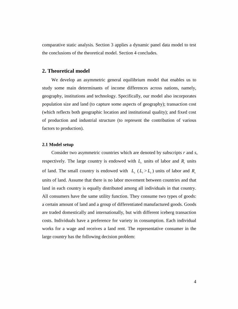
2.1 Model setup

Consider two asymmetric countries which are denoted by subscripts r and s,

respectively. The large country is endowed with rL units of labor and rR units

of land. The small country is endowed with sL ( rL > sL ) units of labor and sR

units of land. Assume that there is no labor movement between countries and that

land in each country is equally distributed among all individuals in that country.

All consumers have the same utility function. They consume two types of goods:

a certain amount of land and a group of differentiated manufactured goods. Goods

are traded domestically and internationally, but with different iceberg transaction

costs. Individuals have a preference for variety in consumption. Each individual

works for a wage and receives a land rent. The representative consumer in the

large country has the following decision problem:

5

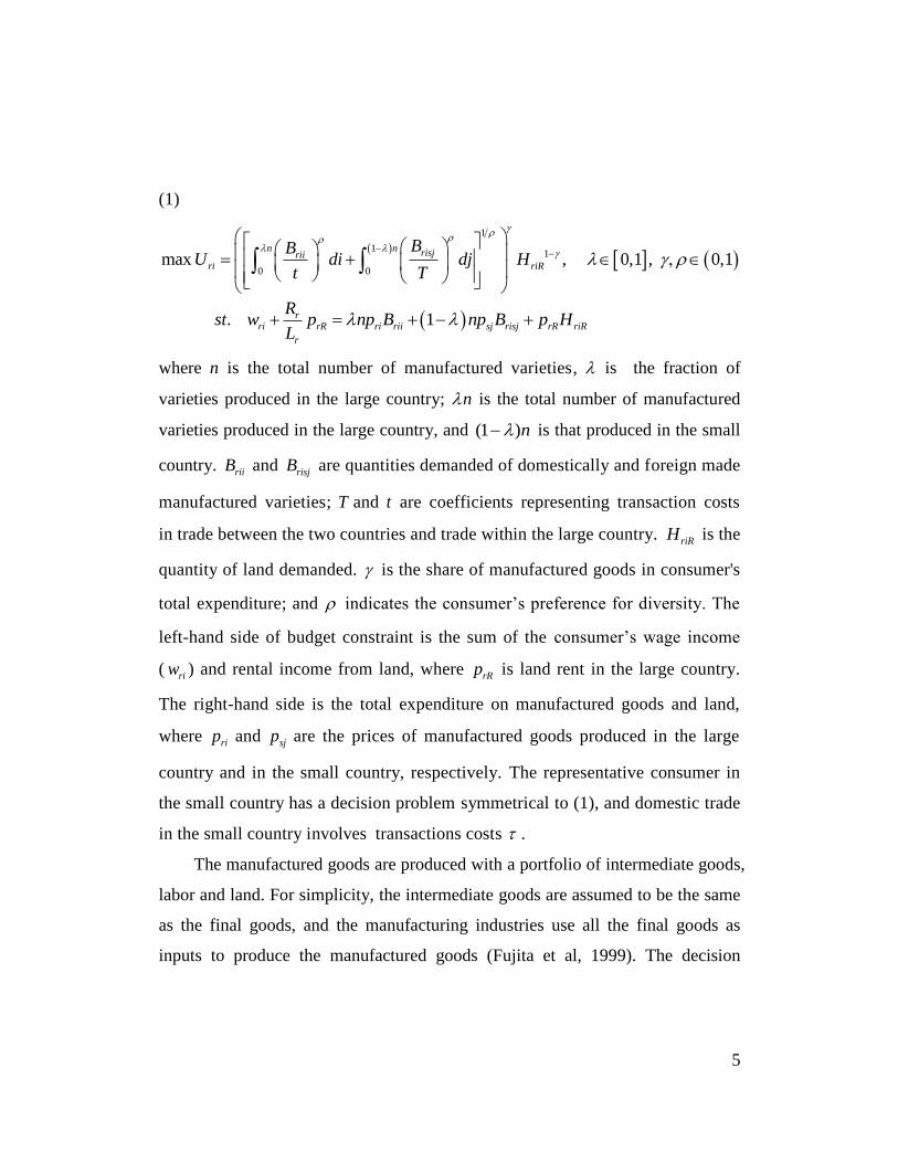
(1)

1

11

0 0max , 0,1 , 0,1

n n risjriiri riR

BBU di dj H

t T

. 1rri rR ri rii sj risj rR riR

r

Rst w p np B np B p H

L

where n is the total number of manufactured varieties, is the fraction of

varieties produced in the large country; n is the total number of manufactured

varieties produced in the large country, and (1 )n is that produced in the small

country. riiB and risjB are quantities demanded of domestically and foreign made

manufactured varieties; T and t are coefficients representing transaction costs

in trade between the two countries and trade within the large country. riRH is the

quantity of land demanded. is the share of manufactured goods in consumer's

total expenditure; and indicates the consumer’s preference for diversity. The

left-hand side of budget constraint is the sum of the consumer’s wage income

( riw ) and rental income from land, where rRp is land rent in the large country.

The right-hand side is the total expenditure on manufactured goods and land,

where rip and sjp are the prices of manufactured goods produced in the large

country and in the small country, respectively. The representative consumer in

the small country has a decision problem symmetrical to (1), and domestic trade

in the small country involves transactions costs .

The manufactured goods are produced with a portfolio of intermediate goods,

labor and land. For simplicity, the intermediate goods are assumed to be the same

as the final goods, and the manufacturing industries use all the final goods as

inputs to produce the manufactured goods (Fujita et al, 1999). The decision

6

problem facing a representative firm producing the manufactured good i in the

large country is:

(2)

max 1ri ri ri ri rii sj risj ri ri rR riRp q np Z np Z w l p A ,

11

0 0. , 0,1 , , , 0,1

n n risjriiri ri riR

ZZst q di dj l A

t T

.

The meaning of (2) is that the representative firm uses various factors to

produce a target output in order to maximize profit. riiZ and risjZ are respectively

the quantities of intermediate good i produced domestically and intermediate

good j produced in the small country and shipped to large country. ril and riRA

are the demand of labor and land. is the share of intermediate goods in the

firm's total expenditure, and is the cost share of land input. and reflect

some features of the economic structure. For instance, a high and a low

indicate a higher level of dependence on intermediate manufactured input (or

capital), and therefore a more industrialized economy; conversely a low and a

high indicate a higher level of dependence on land, and therefore a more

agricultural economy.

We assume that the production technology used by the firms has the

property of increasing returns in scale. Denoting the fixed and marginal input

combinations of the representative firm in the large country as f and , and

their price index as rP , we can write the firm’s total costs as:

(3) , , 0ri ri rC f q P f .

The decision problem for the representative producer in the small country is

symmetrical to (2). To facilitate comparison, we use and to denote the cost

7

share of intermediate input and that of land input in manufacturing in the small

country. Moreover, we denote the fixed and marginal input combinations of the

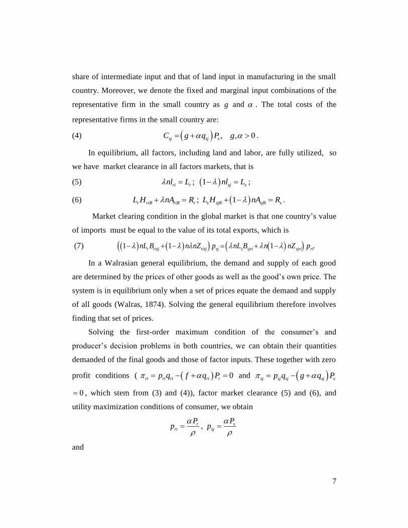
representative firm in the small country as g and . The total costs of the

representative firms in the small country are:

(4) , , 0sj sj sC g q P g .

In equilibrium, all factors, including land and labor, are fully utilized, so

we have market clearance in all factors markets, that is

(5) ri rnl L ; 1 sj snl L ;

(6) r riR riR rL H nA R ; 1s sjR sjR sL H nA R .

Market clearing condition in the global market is that one country’s value

of imports must be equal to the value of its total exports, which is

(7) 1 1 1r risj risj sj s sjri sjri rinL B n nZ p nL B n nZ p .

In a Walrasian general equilibrium, the demand and supply of each good

are determined by the prices of other goods as well as the good’s own price. The

system is in equilibrium only when a set of prices equate the demand and supply

of all goods (Walras, 1874). Solving the general equilibrium therefore involves

finding that set of prices.

Solving the first-order maximum condition of the consumer’s and

producer’s decision problems in both countries, we can obtain their quantities

demanded of the final goods and those of factor inputs. These together with zero

profit conditions ( 0ri ri ri ri rp q f q P and sj sj sj sj sp q g q P

0 , which stem from (3) and (4)), factor market clearance (5) and (6), and

utility maximization conditions of consumer, we obtain

rri

Pp

, s

sj

Pp

and

8

11

r rirR

r

L wp

R

, 1

1

s sj

sR

s

L wp

R

.

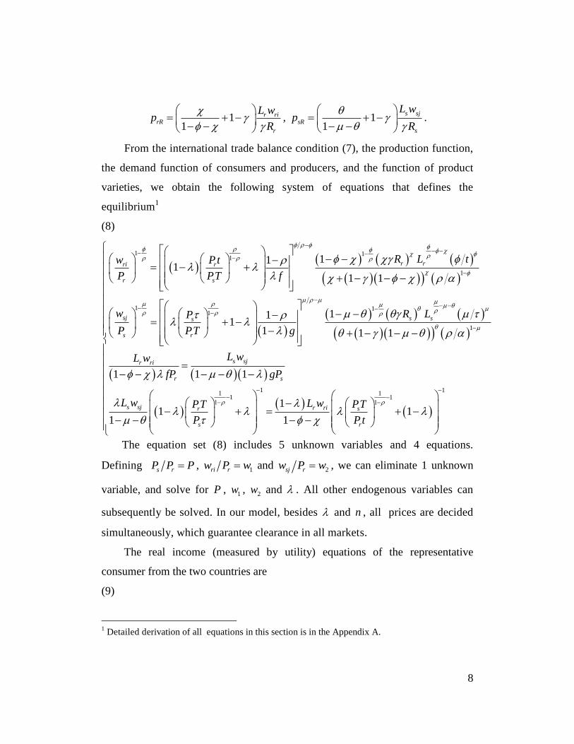
From the international trade balance condition (7), the production function,

the demand function of consumers and producers, and the function of product

varieties, we obtain the following system of equations that defines the

equilibrium1

(8)

1 11

1

1 11

111

1 1

111

1

r rri r

r s

sj s ss

s r

R L tw Pt

P PT f

w R LP

P PT g

1

1 11 1

1 11 1

1 1

1 1 1

11 1

1 1

s sjr ri

r s

s sj r ri sr

s r

L wL w

fP gP

L w L w PTPT

P Pt

The equation set (8) includes 5 unknown variables and 4 equations.

Defining s rP P P , 1ri rw P w and 2sj rw P w , we can eliminate 1 unknown

variable, and solve for P , 1w , 2w and . All other endogenous variables can

subsequently be solved. In our model, besides and n , all prices are decided

simultaneously, which guarantee clearance in all markets.

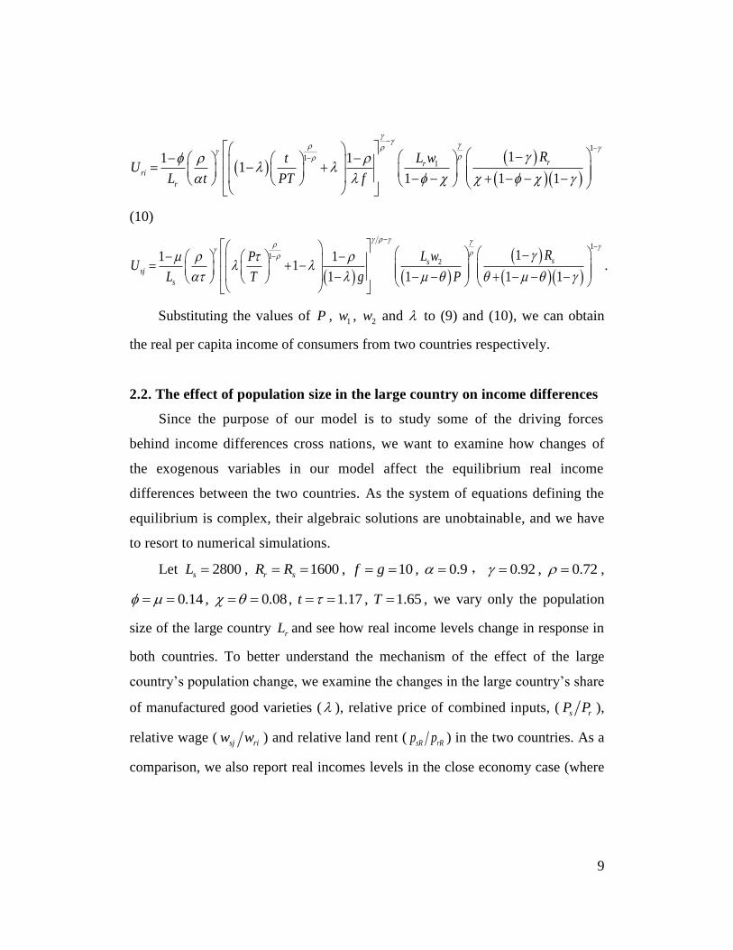
The real income (measured by utility) equations of the representative

consumer from the two countries are

(9)

1 Detailed derivation of all equations in this section is in the Appendix A.

9

1

11

11 11

1 1 1

rrri

r

RL wtU

L t PT f

(10)

1

12

11 11

1 1 1 1

sssj

s

RL wPU

L T g P

.

Substituting the values of P , 1w , 2w and to (9) and (10), we can obtain

the real per capita income of consumers from two countries respectively.

2.2. The effect of population size in the large country on income differences

Since the purpose of our model is to study some of the driving forces

behind income differences cross nations, we want to examine how changes of

the exogenous variables in our model affect the equilibrium real income

differences between the two countries. As the system of equations defining the

equilibrium is complex, their algebraic solutions are unobtainable, and we have

to resort to numerical simulations.

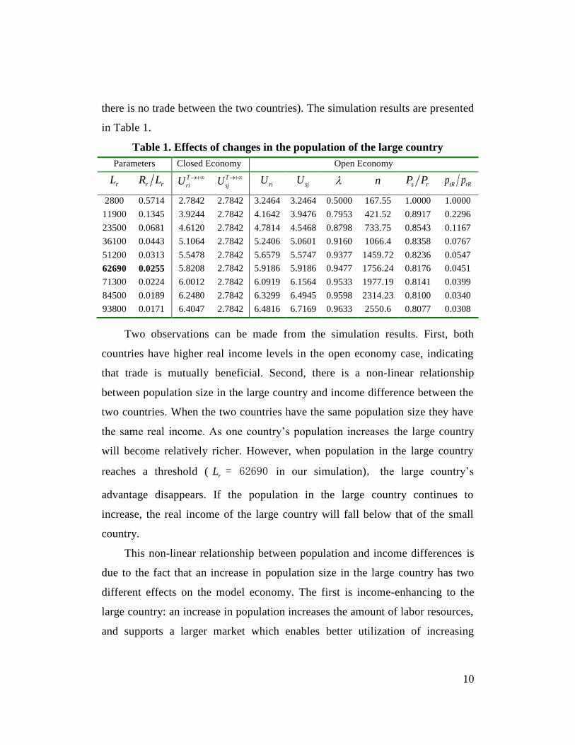
Let 2800sL , 1600r sR R , 10f g , 0.9 ， 0.92 , 0.72 ,

0.14 , 0.08 , 1.17t , 1.65T , we vary only the population

size of the large country rL and see how real income levels change in response in

both countries. To better understand the mechanism of the effect of the large

country’s population change, we examine the changes in the large country’s share

of manufactured good varieties ( ), relative price of combined inputs, ( s rP P ),

relative wage ( sj riw w ) and relative land rent ( sR rRp p ) in the two countries. As a

comparison, we also report real incomes levels in the close economy case (where

10

there is no trade between the two countries). The simulation results are presented

in Table 1.

Table 1. Effects of changes in the population of the large country

Parameters Closed Economy Open Economy

rL r rR L T

riU T

sjU riU sjU n s rP P sR rRp p

2800 0.5714 2.7842 2.7842 3.2464 3.2464 0.5000 167.55 1.0000 1.0000

11900 0.1345 3.9244 2.7842 4.1642 3.9476 0.7953 421.52 0.8917 0.2296

23500 0.0681 4.6120 2.7842 4.7814 4.5468 0.8798 733.75 0.8543 0.1167

36100 0.0443 5.1064 2.7842 5.2406 5.0601 0.9160 1066.4 0.8358 0.0767

51200 0.0313 5.5478 2.7842 5.6579 5.5747 0.9377 1459.72 0.8236 0.0547

62690 0.0255 5.8208 2.7842 5.9186 5.9186 0.9477 1756.24 0.8176 0.0451

71300 0.0224 6.0012 2.7842 6.0919 6.1564 0.9533 1977.19 0.8141 0.0399

84500 0.0189 6.2480 2.7842 6.3299 6.4945 0.9598 2314.23 0.8100 0.0340

93800 0.0171 6.4047 2.7842 6.4816 6.7169 0.9633 2550.6 0.8077 0.0308

Two observations can be made from the simulation results. First, both

countries have higher real income levels in the open economy case, indicating

that trade is mutually beneficial. Second, there is a non-linear relationship

between population size in the large country and income difference between the

two countries. When the two countries have the same population size they have

the same real income. As one country’s population increases the large country

will become relatively richer. However, when population in the large country

reaches a threshold ( rL = 62690 in our simulation), the large country’s

advantage disappears. If the population in the large country continues to

increase, the real income of the large country will fall below that of the small

country.

This non-linear relationship between population and income differences is

due to the fact that an increase in population size in the large country has two

different effects on the model economy. The first is income-enhancing to the

large country: an increase in population increases the amount of labor resources,

and supports a larger market which enables better utilization of increasing

11

returns to scale and a greater variety of manufactured goods produced.1 The

second is income-limiting for the large country: the increase in population

reduces per capita land, which reduces per capita real income in the large

country directly (as land is a consumption item), and indirectly (due to

decreasing returns to labor when land is fixed). Initially the income enhancing

effect dominates, and the large country gains relatively more than the small

country. However, when the population exceeds the threshold value, the income-

limiting effect becomes more severe in the large country and the population

advantage turns into a population burden.

2.3. The effects of other variables on income differences

Obviously (relative) population size is not the only factor determining cross-

country income differences. While a large country has an advantage before its

population reaches a critical threshold, there are other factors which strengthen or

weaken this advantage. Thus a populous country may be rich (e.g., the US, Japan)

or not (e.g., China, India) depending on the joint effects of many forces. In the

following, we consider six factors affecting income differences cross countries,

namely, international transaction costs ( T ), domestic transaction costs ( t ),

technology ( f ), natural resources ( rR ), the industry’s dependence on natural

resources ( ) and the degree of industrial linkage ( ). Similar to our analysis of

the population effect, we still resort to numerical simulations. Specifically, we

start with a given set of parameter values and obtain real income levels in both

countries; then we give different values to only the parameter in question, and

obtain different real income levels. Based on the pattern of responses in real

1 As population in the large country increases, both countries produce more goods, but the share of

varieties produced in the large country increases.

12

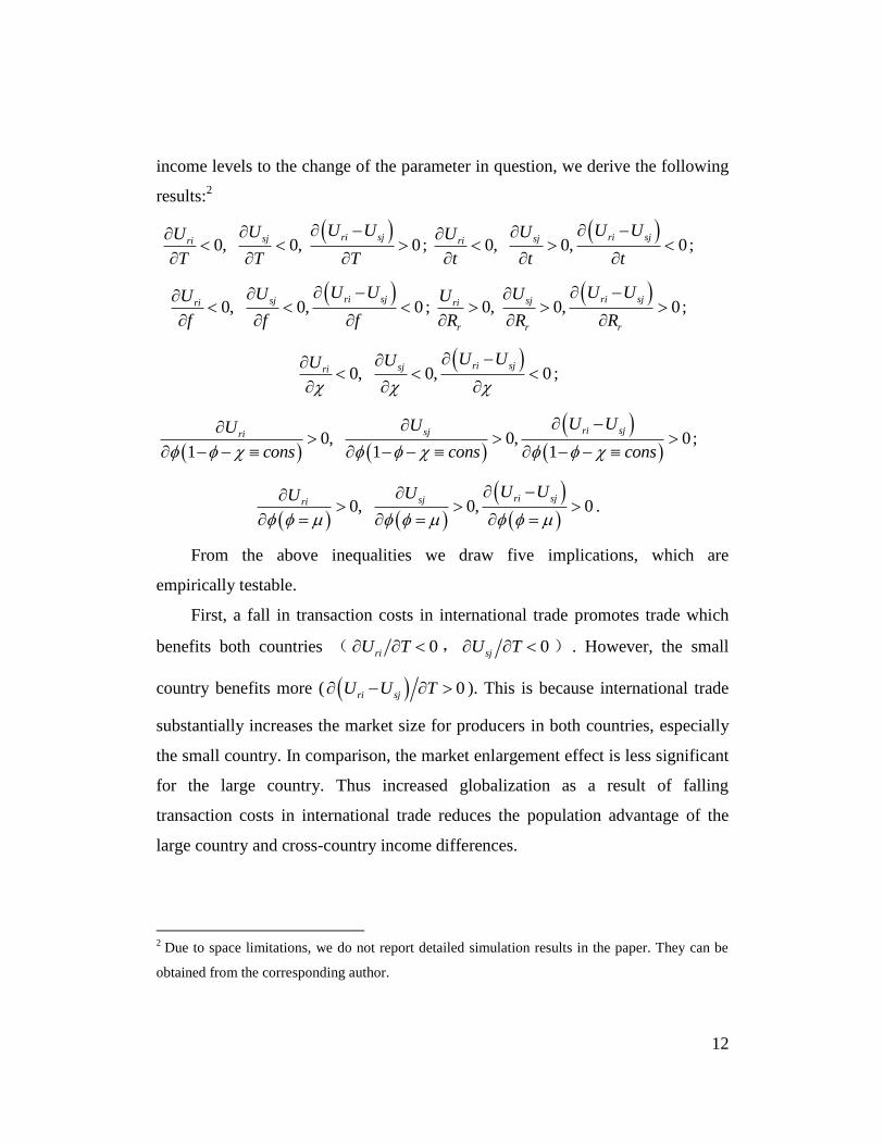
income levels to the change of the parameter in question, we derive the following

results:2

0, 0, 0

ri sjsjriU UUU

T T T

;

0, 0, 0

ri sjsjriU UUU

t t t

;

0, 0, 0

ri sjsjriU UUU

f f f

;

0, 0, 0

ri sjsjri

r r r

U UUU

R R R

;

0, 0, 0

ri sjsjriU UUU

;

0, 0, 01 1 1

ri sjsjriU UUU

cons cons cons

;

0, 0, 0ri sjsjri

U UUU

.

From the above inequalities we draw five implications, which are

empirically testable.

First, a fall in transaction costs in international trade promotes trade which

benefits both countries （ 0riU T ， 0sjU T ） . However, the small

country benefits more ( 0ri sjU U T ). This is because international trade

substantially increases the market size for producers in both countries, especially

the small country. In comparison, the market enlargement effect is less significant

for the large country. Thus increased globalization as a result of falling

transaction costs in international trade reduces the population advantage of the

large country and cross-country income differences.

2 Due to space limitations, we do not report detailed simulation results in the paper. They can be

obtained from the corresponding author.

13

Second, a fall in domestic transaction costs in the large country increases the

large country’s real income ( 0riU t ), but has a small negative effect on the

small country3, therefore the large country’s relative income increases. It should

be noted here that transaction costs in our model can be interpreted to encompass

not only transportation costs, but also other factoring influencing efficiency in

market transaction, in particular, institutional factors such as rule of law, security

property rights and contract enforcement. If a large poor country (e.g., China and

India) reduces its domestic transaction costs through for example reforms that

improve domestic institutions, it will capture most of the resulting benefits with

little spillover, and consequently narrowing cross-country income differences.

Third, technology and natural resources are important determinants of real

income. If the large country has a low level of technology (a large f ) or a low

level of per capita natural resources (small r rR L ), it will have a low level of real

income. An improvement in technology or a discovery of more natural resources

in the large country not only benefits the large country and increases its real

income relative to the small country ( ( ) 0rj sjU U f , ( ) 0rj sj rU U R ),

but also has a positive spillover effect through trade on the small country, i.e.,

0sjU f , 0sj rU R .

Fourth, a high level of dependence of production on natural resources (a

large ) is not favorable to a country. When a country is in transition from a

natural resource-intensive industrial structure to a labor-intensive or capital-

3 A reduction in domestic transaction costs has two effects. First, it increase the total number of

good varieties, which benefits both countries through international trade. Second, it may induce

industries in another country to move to the country with reduced domestic transaction cost. As

shown in Table B.2 in the Appendix B, as domestic transaction costs are reduced, the number of

goods produced in another country ( 1 n ) falls.。

14

intensive industrial structure, the country is likely to experience a significant

increase in per capita real income, and extends the benefits to other countries

through trade. indicates the large country’s degree of dependence on land or

natural resource. indicates the large country’s degree of dependence on capital

(or intermediate inputs). If remains unchanged, and falls, it means that the

large country is transitioning from an land-intensive agricultural economy to a

labor-intensive handicraft economy. On the other hand, if increases and

1 remains unchanged (1 cons ), then must move in opposite

direction to . This means that the economic structure in the large country is

moving from land-intensive agriculture to capital-intensive modern

manufacturing. 0ri sjU U and 1 0ri sjU U cons

imply that if one country has transitioned from an agricultural economy to a

handicraft economy or a modern manufacturing economy, whereas another

country remains in an agricultural economy, then the former will enjoy a

significantly higher per capital income.

Fifth, the degree of industrial linkage has a positive effect on both countries’

per capita real income, with the large country benefiting more from higher levels

of industrial linkage. has two meanings. Apart from the economic structure

mentioned above, it can also indicate the linkages between firms and the degree of

roundaboutness in production. In this paper, capital is intermediate input, which

reflects the roundaboutness in production in the Böhm-Barwerkian sense. The

degree of roundaboutness is related to the number of intermediate varieties. To

some degree, indicates the intensity of intermediate goods use. However, since

an increase in also increases the number of intermediate input varieties, thus it

also reflects the extent to intermediate input use. The larger the number of

intermediate input used, the longer the roundabout production process. Since the

15

large country produces more varieties of intermediate goods, when the degree of

linkages between firms increases, the large country will purchase more

intermediate inputs from its domestic market, thus saving international transaction

costs and lowering costs of production. This may widen the real income

differences between the large country and the small country

( 0ri sjU U ).

3. Empirical Analysis

Our theoretical model above has shown the existence of a large country

advantage (before the threshold population level has been reached), however

there are many other factors constraining the development of a large country. If

the constraining factors are significant, the large country advantage will be

offset and a large country is possibly poorer than a small country. Indeed there

are many large poor countries in the world, giving an impression that a larger

population is associated of poverty. However, first impression can often be

deceiving. In this section, we test the main conclusions of our theoretical model,

including the existence of the large country advantage.

3.1 Model setup and choice of variables

Although the subject of our paper concerns income growth, but our

theoretical model is one of spatial allocation, and we use comparative statics to

derive our conclusions. In the empirical analysis, we therefore try to exclude the

effect of time per se on the economic system. Based on the conclusions of our

theoretical model, we choose the following empirical model:

(11)

1 2 3 4 5

6 7

cosit it it it it it

it it i it

gdpdev popshare urban export road t energy

dust tech

.

16

Where i denotes country or region, t denotes time, i is unobservable

country/region effects, it is random error.

The dependent variable in the model, gdpdev, measures the deviation of a

country’s average per capita real income from the world mean. Barro and Sala-

i-Martin (1992) use the cross-country deviation of real per capital income to

indicate cross-country income differences. In our analysis, gdpdev is

calculated as the ratio of each country’s per capita real GDP (constant 1990

PPP $) and the world average per capita real GDP.

Independent variable popshare is a country’s population as a share of the

world total. This variable measures population distribution, and is the key

explanatory variable of our model. Since population is an important production

input, and labor income in turn determines demand, a country’s GDP is likely

to be positively correlated with its population. We will also use laborshare

(which is a country’s total labor employed as a share of the world total labor

employed), as an alternative indicator of population size.

Independent variable urban is the deviation of a country’s urban

population share from the world average. The share of urban population is a

common measure of urbanization and reflects also the degrees of

industrialization. Since industries and services are labor-intensive industries

which tend to concentrate in urban areas, a higher urban indicates that

industrial products and services take a larger share in the total output, whereas

agriculture takes a small share. Thus urban to some extent reflects the

importance of non-agricultural activities in the economy structure.

Independent variable export is ratio of a country’s the share of exports in

GDP to the world average. This is a measure of trade openness. The degree of

trade openness is associated with country size. A large country tends to have a

lower degree of trade openness because it has a large domestic economy and

17

residents can purchase more goods and services domestically. The US is

considered to be a very open economy, however, its average trade openness

over our sample periods is 11.02. The average trade openness for China is

27.37, however, the corresponding figure for Singapore is 198.08. Clearly, a

small country tends to be more deeply immersed in international trade. Apart

from population size, a country’s geographic location (distance to ocean,

capacity of ports), international transportation and other transaction costs also

affect a country’s trade openness.

Independent variable roadcost is the ratio of a country’s energy

consumption per unit of GDP (PPP) by the road sector to the world average. It to

some degree reflects cross-country differences in domestic transportation costs.

Since a large portion of the transaction costs is unobservable, domestic transaction

costs and the extent of market development is very hard to be measured. Of the

measurable transportation costs, it is hard to be classified by type. We adopt

energy use by the road transportation sector as a proxy of domestic transportation

costs because it reflects millage travelled, which in turn is closely related vehicle

depreciation and wage costs of drivers.

Independent variables land and energy measure cross country difference in

per capita natural resources. land is the ratio of a country’s per capita land area to

the world average. energy is the ratio of a country’s per capita production of

energy equivalent to the world average. Since land in many countries includes

deserts, jungles, high altitude mountains and plateaus, that are not suitable for

human habitation or production, land is not an accurate measure of resources.

Some scholars recommend the use of resource reserves per unit of land, but

resource reserves are also hard to be measured accurately. Moreover, from the

economic perspective, reserves do not reflect the difficulty and costs of resource

extraction. Since resources will only be extracted up to the point where the margin

benefit of extracting equals its marginal costs, resource output and value in each

18

country can better reflect differences in resource endowment. Therefore we use

energy to measure cross country resource differences.

Independent variable densitysq and dust measure the degree of crowdedness

due to land scarcity. densitysq is calculated by taking the ratio of a country’s

population density (population per unit of land) to the world average, then

squaring the ratio. Since population is positively correlated to GDP, if the

coefficient of densitysq in our estimation turns out to be negative, it suggests a

inverted U relationship between population and per capita GDP. dust is the ratio

of a country’s per cubic meter total suspended particulates (TSP) to the world

average. If the coefficient of dust is negative, it would suggest that environment

degradation and overcrowding has a negative impact on economic development.

Independent variable tech is ratio of a country’s energy use per unit of GDP

(constant 1990 PPP $) to the world average. As a rule countries with high levels

energy efficiency also have advanced technologies albeit energy efficiency also

reflects superiority of management practices.

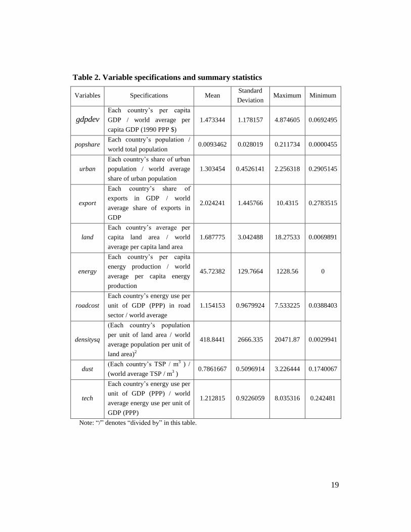
3.2 Data sources and summary statistics

Our empirical analysis is based on a panel data set covering 91 countries

over the period of 1994-2011. The main data source is the World Bank. Table

2 lists all variables, their definitions and summary statistics.

19

Table 2. Variable specifications and summary statistics

Variables Specifications Mean Standard

Deviation Maximum Minimum

gdpdev

Each country’s per capita

GDP / world average per

capita GDP (1990 PPP $)

1.473344 1.178157 4.874605 0.0692495

popshare Each country’s population /

world total population 0.0093462 0.028019 0.211734 0.0000455

urban

Each country’s share of urban

population / world average

share of urban population

1.303454 0.4526141 2.256318 0.2905145

export

Each country’s share of

exports in GDP / world

average share of exports in

GDP

2.024241 1.445766 10.4315 0.2783515

land

Each country’s average per

capita land area / world

average per capita land area

1.687775 3.042488 18.27533 0.0069891

energy

Each country’s per capita

energy production / world

average per capita energy

production

45.72382 129.7664 1228.56 0

roadcost

Each country’s energy use per

unit of GDP (PPP) in road

sector / world average

1.154153 0.9679924 7.533225 0.0388403

densitysq

(Each country’s population

per unit of land area / world

average population per unit of

land area)2

418.8441 2666.335 20471.87 0.0029941

dust (Each country’s TSP / m

3 ) /

(world average TSP / m3 )

0.7861667 0.5096914 3.226444 0.1740067

tech

Each country’s energy use per

unit of GDP (PPP) / world

average energy use per unit of

GDP (PPP)

1.212815 0.9226059 8.035316 0.242481

Note: “/” denotes “divided by” in this table.

20

3.3. Estimation method and results

Usually, a country’s income level in the current period depends on its

income level in the last period. A poor country does not suddenly turn into a rich

country or vice versa. Therefore we introduce lagged gdpdev to equation (11)

and make it into a dynamic panel:

(12)

, 1 1 2 3 4

5 6 7

cosit i t it it it it

it it it i it

gdpdev gdpdev popshare urban export road t

energy dust tech

A dynamic panel not only solves the problem of serial correlation but also

addresses the problem of endogenity between independent variables. Since the

economic system in essence is a general equilibrium, the variables are

interdependent, which gives rise to the endogeneity problem. In this case, the

OLS estimator is biased and inconsistent. Our empirical model has this problem

as well. In addition, the endogeneity problem arises when there is omitted variable

due to unobtainable data or unmeasurable variables. Since we have only limited

data from the World Bank, our model has the problem of omitted variables. These,

together with possible measurement errors in the data, imply that all OLS

estimates would be biased and inconsistent.

The data period in our analysis is 18 years. In the short run, popshare may be

considered to be exogenous. However, over a longer term, population is affected

by birth rate, mortality rate and migration rate, which in turn are affected by per

capita GDP. Thus popshare and gdpdev are jointly determined. urban reflects

changes in economic structure, and export reflects changes in trade openness.

Both are influenced by per capita GDP. If per capita GDP in a country increases,

its domestic demand and consumption structure will change in a way to facilitate

the transition from an agricultural economy to an industrialized economy. An

increase in GDP also implies larger production capacity and improvement in

21

transportation, therefore lowering transportation costs, and promoting domestic

and international trade. Thus, gdpdev, urban, export and roadcost are

interdependent as well. A country’s energy production is also affected by its level

of economic development and industrialization. Countries with higher levels of

per capita GDP, industrialization and urbanization have higher demand for energy,

which stimulates energy production. Since energy production itself is energy

intensive, higher energy production may also lead to higher CO2 emission and

higher total suspended particulates in the air. Thus, energy, dust, urban and

gdpdev are interdependent. Finally, due to knowledge spillover effects, a

country’s population size, urbanization and degree of industrialization may also

affect the country’s energy efficiency and technology level. Thus, popshare,

urban, and tech may also be interdependent. All these complex endogeneity

problems may be addressed by dynamic panel Generalized method of moments

(GMM) estimation.

Either the one-step GMM estimator or the two-step GMM estimator can be

used. Windmeijer (2005) shows that estimated asymptotic standard errors of the

two-step GMM estimator may be downward biased in small samples due to the

use of estimated parameters in constructing the weight matrix. He therefore

recommends the use of a correction term generated by a Taylor expansion.

However since this method leads to an asymptotically inefficient GMM estimator,

one-step GMM estimator is more widely used (Bond, 2002). According to

Blundell and Bond (2000), Blundell and Windmeijer (2002), one-step system

GMM estimator is more precise than the standard first-step differenced GMM

estimator. In this paper, we apply the one-step system GMM estimation (Arellano

and Bover, 1995 and Blundell and Bond, 1998). As a robust check, we also report

results from the two-step system GMM estimation. The estimation results of

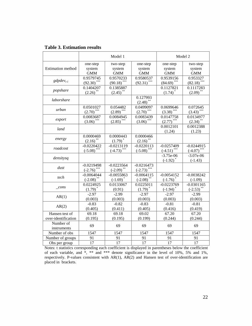
model (12) are presented in Table 3.

22

Table 3. Estimation results

Model 1 Model 2

Estimation method

one-step

system

GMM

two-step

system

GMM

one-step

system

GMM

one-step

system

GMM

two-step

system

GMM

gdpdevt-1 0.9579745

(92.30) ***

0.9570233

(90.18) ***

0.9580537

(92.31) ***

0.9539156

(84.69) ***

0.953327

(82.18) ***

popshare 0.1404207

(2.26) **

0.1385887

(2.45) **

0.1127821

(1.74) *

0.1117283

(2.09) **

laborshare 0.127993

(2.48) **

urban 0.0501027

(2.70) ***

0.054482

(2.89) ***

0.0499097

(2.70) ***

0.0699646

(3.38) ***

0.072645

(3.43) ***

export 0.0083687

(3.06) ***

0.0084945

(2.85) ***

0.0083439

(3.06) ***

0.0147758

(2.77) ***

0.0134977

(2.34) **

land 0.0012101

(1.24)

0.0012388

(1.23)

energy 0.0000469

(2.16) **

0.0000443

(1.79) *

0.0000466

(2.16) **

roadcost -0.0220422

(-5.08) ***

-0.0213119

(-4.73) ***

-0.0220113

(-5.08) ***

-0.0257409

(-4.51) ***

-0.0244915

(-4.07) ***

densitysq -3.75e-06

(-1.92) *

-3.07e-06

(-1.43)

dust -0.0219498

(-2.76) ***

-0.0223564

(-2.09) **

-0.0216473

(-2.73) ***

tech -0.0064044

(-2.08) **

-0.0055863

(-1.69) *

-0.0064115

(-2.08) **

-0.0054152

(-1.76) *

-0.0038242

(-1.09)

_cons 0.0224925

(1.79) *

0.0133067

(0.91)

0.0225011

(1.79) *

-0.0223769

(-1.94) *

-0.0301165

(-2.53) **

AR(1) -2.97

(0.003)

-2.99

(0.003)

-2.97

(0.003)

-2.97

(0.003)

-2.99

(0.003)

AR(2) -0.83

(0.405)

-0.82

(0.411)

-0.83

(0.405)

-0.81

(0.416)

-0.81

(0.419)

Hansen test of

over-identification

69.18

(0.195)

69.18

(0.195)

69.02

(0.199)

67.20

(0.244)

67.20

(0.244)

Number of

instruments 69 69 69 69 69

Number of obs 1547 1547 1547 1547 1547

Number of groups 91 91 91 91 91

Obs per group 17 17 17 17 17

Notes: t statistics corresponding each coefficient is displayed in parentheses below the coefficient

of each variable, and *, ** and *** denote significance in the level of 10%, 5% and 1%,

respectively. P-values consistent with AR(1), AR(2) and Hansen test of over-identification are

placed in brackets.

23

Table 3 reports test statistics for residual serial correlation AR(1), AR(2) and

over-identification and their corresponding p-values. It is clear that the null

hypothesis of no first-order serial correlation is rejected at 1% level, whereas the

null hypothesis of no AR(2) cannot be rejected. In all of our estimations, we use

69 instrumental variables to estimate 8 explanatory variables, giving rise to

multiple over-identification moment conditions. The Hansen test statistics for all

models has a p-value of greater than 10%, indicating the null hypothesis of valid

instruments cannot be rejected. This implies that our choice of instrumental

variables and their lag orders are appropriate.

From Table 3, we see that lagged income difference (gdpdevt-1) has a

positive and significant coefficient of 0.95. This indicates that much of cross-

country income difference is determined by historical factors. Nature does not

make jumps (Marshall, 1920), neither do human societies. There is clear path-

dependence in economic development. Apart from the factors analyzed in this

paper, a country’s development is influenced by many other factors including

existing market potential, per capita capital stock, stock of knowledge and human

capital accumulation, social institutions, and other “historical stock” (Acemoglu

and Zilibotti, 1997). Since these factors do not change suddenly, a country’s per

capita GDP can only grow on the basis of its previous level.

The variable of our most interest, a country’s population share (popshare)

has a positive and significant coefficient in all models. This supports our

theoretical model’s conclusion that population size has a positive impact on a

country’s per capita real income (before a population threshold level has been

reached). Although this conclusion does not seem to match our casual

observation, we consider the coefficient of 0.2 may in fact underestimate the

extent of the large country advantage. This is because the large country advantage

is likely to be a long term influence, however we have only 18 years of data. If we

take China and India as large country examples, these two countries are currently

24

poor, but during the 1000 years before the modern era, they were among the

richest in the world.

There are many reasons why the large country advantage may be offset. In

our theoretical model, a number of factors interact to undermine the large country

advantage, including trade openness, crowdedness due to over-population, under-

developed domestic market and high transaction costs, high dependence on land

and natural resources, low levels of technology, etc. The effects of these variables

can be seen from Table 3.

Trade openness (export) has a positive effect on income. As mentioned

before, in a closed economy, the income difference between the large country and

the small country is very big. When international trade takes place, the large

country advantage will spill over to the small country, leading to a narrowing of

income differences. However, even with international trade, if the international

transaction costs are high, the large country will still enjoy higher income. With

the falling international transaction costs, trade volume will increase, and the

degree of openness for the small country will rise faster. As a result, income

differences narrow. In comparison, since a large country produces more product

varieties and its residents can purchase more goods domestically, its benefit from

international trade is relatively smaller. The estimation results support our

theoretical prediction.

Domestic transaction costs (roadcost) have a significantly negative impact

on a country’s income. Our theoretical model predicts that a fall in a country’s

domestic transaction costs will increase the country’s per capita real income, but

has a tiny negative impact on its trade partner. It should be noted that although

fuel consumption by the road transportation sector is a good proxy of

transportation costs, it does not cover all domestic transaction costs. The scope of

transaction costs is large, including social customs, law and regulations, market

development, corporate governance, property right systems etc. However these

25

factors are mostly un-measurable. Since we apply dynamic panel GMM

estimation, the problems associated with omitted variables and measurement

errors are addressed by lagged variables. The results in Table 3 support the

conclusion that an improvement in domestic transaction efficiency enhances a

country’s international competitiveness.

A country’s urban population as a share total population (urban) has

significant positive effect on per capita GDP. The share of urban population

reflects a country’s degree of industrialization. Usually a higher urban indicates a

high proportion of non-agricultural activities in a country’s economy. Agriculture

is a sector highly dependent on land. In countries with high proportions of

agricultural population, the level of division of labor tends to be low. Farmers

self-provide agricultural products and sell the surplus to the market. This low

level of division of labor is not conducive to economic development. The

transition from agricultural-based to industry-based economic structure in poor

countries will narrow the income differences between these countries and the rich

countries.

The estimated coefficient of energy use per unit of GDP (tech) is negative

and significant. One the one hand, tech measures technological differences:

countries with more advance technologies tend to consume less energy to produce

a unit of GDP. On the other hand, tech to some extent describes the structure of

the economy. If a country’s economy is dominated by energy-intensive industries

such as electricity generation, mining and steel making, then it will have a high

value of tech. The negative sign of the estimated coefficient suggests that higher

technology levels and low energy intensity are associated with higher per capita

real income.

A country’s per capita land area (land) has a positive coefficient but is not

significant. Although land is an objective measure of per capital land area, it does

not accurately capture the distribution of resources. Land of the same size may

26

differ in soil fertility and in resources. It is thus not entirely surprising to find land

to be an insignificant explanatory variable for income differences.

A country’s energy production (energy) has a positive and significant effect

on income differences, but the effect is small. Resource endowment contributes to

per capita GDP, but it is possible to have the “resource curse”, resulting in a small

net positive effect.

A country’s TSP measure in cities (dust) has a negative and significant effect

on income differences. TSP measure may be related to industrial production and

energy consumption. High levels of TSP may affect economic development

through two channels: air pollution harms the health status of residents, and

induce local enterprise to move elsewhere. Secondly, local governments and

enterprises need to devote more resources to clean the environment, pushing up

the costs faced by businesses. The negative coefficient of dust implies that

excessive industry and population density creates over-crowded environment

which has a negative impact on per capita GDP. This result is also supported by a

negative and significant coefficient of densitysq.

4. Conclusion

In this paper we have studied various factors affecting cross-country income

differences within the framework of a spatial general equilibrium model. We have

also empirically tested the conclusions of our theoretical model using data of 91

countries (regions) over the period of 1994-2011. The main conclusions are as

follows.

First, cross-country income differences are determined by many different

factors. A country’s population size and per capita natural resource endowment

has an important impact on cross-country income differences. This conclusion is

derived from our theoretical model and supported by our empirical test. We can

also find much supporting evidence outside our sample period. China and India

27

are historically populous countries and were among the wealthiest in the world

during the 1000 or so years before the modern era.

Second, falling international transaction cost and increasing trade openness

tend to reduce cross-country income differences, whereas falling domestic

transaction costs tend to increase them. Notably, some economists have identified

significant club convergence. Mankiw et al (1992) find evidence of convergence

at the rate predicted by the augmented Solow model. Kaitila (2004) shows that

real per capita GDP in the EU15 countries converged during the periods 1963-

1973 and 1981-2001. O’Rourke and Williamson (1994) demonstrate that trade

liberalization since the end of 19th

century ushered in an era of economic

convergence. Ireland and Scandinavian countries have gradually caught up with

the older developed countries such as Britain, France and Germany. The income

gap has also narrowed between countries in Latin America and Oceania on the

one hand and the older developed countries on the other (Yang, 2003). However

the income levels of a number of African and South Asian countries still lag far

behind developed countries, in some cases the income gap has even widened. One

explanation for this growth pattern is that transaction costs within the EU have

substantially fallen, and trade openness has also improved for North America,

Latin America and Oceania. In contrast, South Asia, and African countries tend to

be less integrated into the world economy, and their domestic markets are also

under-developed. Our model suggests that when transaction costs within the EU

fall, EU countries develop faster, increasing the income gap between them and

countries outside of the EU. It should be also noted that while markets in many

other countries enjoyed fast development after WWII, some African and South

Asian countries had chosen the paths of central planning with authoritarian

regimes. This led to political instability and high domestic transaction costs. As a

result, their income levels have fallen further behind those of developed countries.

28

Third, a country’s per capita resource endowment and geographical location

have important effects on its per capita income. Countries with high degrees of

trade openness usually enjoy an advantage in maritime transport. This advantage

has a positive impact on these countries’ income. When a country has a large per

capita resource endowment, marginal productivity of labor tends to be large,

which in turn raise per capita real income. In comparison, when per capita

resource is small, people have to adopt intensive farming on limited land,

consequently marginal product of labor is low. Hence, ceteris paribus, per capita

income will be low.

Fourth, a shift of a country’s economic structure from land intensive

production to capital intensive production usually raises per capita real income of

this country. When per capita land resource is small, the shift in economic

structure relaxes the country’s land constraint, enabling extraordinary growth.

Kuznets (1973) argues a high rate of structural shifts is a main characteristic of

modern economic growth. Our model supports this view. Historically, many

populous countries indeed achieved fast economic growth following their

structural shift from agricultural economies to industrial economies. China was a

strong agricultural economy in pre-modern times. At the beginning of the 19th

century, China’s population had reach 300 million, resulting in substantially

smaller per capita arable land area. However, for various reasons, China did not

achieve the structural shift from an agricultural economy to an industrial economy.

Unsurprisingly, China remained a poor country.

29

References

[1] Acemoglu, Daron, and James Robinson, Why Nations Fail: The Origins

of Power, Prosperity, and Poverty. New York: Random House, Crown Publishing,

2012.

[2]Acemoglu, Daron, Simon Johnson and James A. Robinson, Reversal of

Fortune: Geography and Development in the Making of the Modern World

Income Distribution, Quarterly Journal of Economics, 2002, 117, (4), 1231－

1294.

[3]Acemoglu, Daron and F. Zilibotti, Was Prometheus Unbound by Chance?

Risk, Diversification, and Growth, Journal of Political Economy, 1997, 105: 709

－775.

[4]Arellano, M. and O. Bover, Another Look at the Instrumental Variables

Estimation of Errors-component Models, Journal of Econometrics, 1995, 68: 29

－51.

[5]Baldwin, R. , Forslid, R. , Martin, P. , Ottaviano, G. and Robert-Nicoud,

Economic Geography and Public Policy, Princeton University Press, 2003.

[6]Baldwin, R. and Martin, P. , Agglomeration and Regional Growth, The

Handbook of Regional and Urban Economics: Cities and Geography, Vol. 4,

Elsevier Press, 2004.

[7]Baltagi, B. H. , Forecasting with Panal Data, Journal of Forecasting,

2008, 27: 153－173.

[8]Barro, Robert J. and Xavier Sala-i-Martin, Convergence, Journal of

Political Economy, 1992, 100, (2): 223－251.

[9]Blaut, J. M. , The Colonizer's Model of the World: Geographical

Diffusionism and Eurocentric History, New York: The Guilford Press, 1993.

30

[10]Blundell, R. and S. Bond, GMM Estimation with Persistent Panal Data:

an Application to Production Functions, Econometrics Reviews, 2000, 87: 115－

143.

[11]Blundell, R. and S. Bond, Initial Conditions and Moment Restrictions in

Dynamic Panal Data Models, Journal of Econometrics, 1998, 87: 115－143.

[12]Blundell, R. , S. Bond and F. Windmeijer, Estimation in Dynamic Panel

Data Models: Improving on the Performance of the Standard GMM Estimator,

Advances in Econometrics, 2000, 15: 53－91.

[13]Bond, S. , Dynamic Panel Data Models: A Guide to Micro Data

Methods and Practice, CEMMAP Working Paper CWP09/02, Department of

Economics, Institute for Fiscal Studies, London, 2002.

[14]Cassar, A. and Nicolini, R. , Spillovers and Growth in a local Interaction

Model, Annual of Regional Science, 2008, 42: 291－306.

[15]Dupont, Vincent, Do Geographical Agglomeration, Growth and Equity

Conflict?. Papers in Regional Science, 2007, 86, (2): 193－212.

[16]Fujita, M. , Krugman, P. and Venables, A. J. , “The Spatial Economy:

Cities, Regions, and International Trade”, Cambridge: Massachusetts Institute

of Technology, 1999.

[17]Grossman, G. M. and Helpman, E. , Innovation and Growth in the

Global Economy, Cambridge, MA: The MIT Press. 1991.

[18]Helpman, E. , R&D Spillovers and Global Growth, Journal of

International Economics. 1999, 47: 399－428.

[19]Kaitila, Ville, Convergence of Real GDP Per Capita in the EU15,

How Do the Accession Counties Fit in? European Network of Economic

Policy Research Institutes Working Paper， 2004, No. 25.

[20]Kuznets, Simon, Modern Economic Growth: Finding and Reflections,

American Economic Review, 1973, 63, (3): 247－258.

31

[21]Landes, David S. , The Wealth and Poverty of Nations: Why Some Are

So Rich and Some So Poor, New York: W.W. Norton & Company, 1998.

[22]Lin, Justin, The Needham Puzzle: Why the Industrial Revolution Did

Not Originate in China? Economic Development and Cultural Change, 1995,

41: 269－292.

[23]Lin, Justin, Special Topics of the Chinese Economy? 2nd

edition, Beijing:

Beijing University Press, 2012.

[24]Lucas, Robert E. , On the Mechanics of Economic Development,

Journal of Monetary Economics, 1988, 22, (1): 3－42.

[25]Mankiw, N. G. , D. Romer and D. N. Weil, A Contribution to the

Empirics of Economic Growth, The Quarterly Journal of Economics, 1992,

107, (2): 407－437.

[26]Marshall, Alfred, Principles of Economics. 8th ed. London: Macmillan,

1920.

[27]Martin, P. and Ottaviano, G. , Growth and Agglomeration, International

Economic Review, 2001, 42, (4): 947－968.

[28]Martin, P. and Ottaviano, G. , Growth and Agglomeration, CEPR

working paper, No. 1529, 1996.

[29]Martin, P. and Ottaviano, G. , Growing Locations: Industry Location in

A Model of Endogenous Growth, European Economic Review, 1999, (43): 281－

302.

[30]Needham, J. , Science in Traditional China: A Comparative Perspective,

Cambridge, MA: Harvard University Press, 1981.

[31]O’Rourke, K. H. and J. G. , Williamson, Globalization and History.

Cambridge, MA: The MIT Press, 1999.

[32]Romer, Paul M. , Increasing Returns and Long-Run Growth, Journal of

Political Economy, 1986, 94, (5): 1002－1037.

32

[33]Solow, Robert M. , A Contribution to the Theory of Economic Growth,

Quarterly Journal of Economics, 1956, 70, (1): 65－94.

[34]Uzawa, Hirofumi, Optimal Technical Change in an Aggregative Model

of Economic Growth, International Economic Review, 1965, 6: 18－31.

[35]Walras, Léon (1874), Elements of Pure Economics. Homeword, Ill. :

Irwin, 1954.

[36]Wen, James G. . Changes in China’s Territory and Its Impulse to

Come out of the Agrarian Trap: An Economic Geography Approach to the

Needham Puzzle, China Economic Quarterly, 2005, 4, (2): 519－540.

[37]Windmeijer, F. , A Finite Sample Correction for the Variance of Linear

Efficient Two-step GMM Estimators, Journal of Econometrics, 2005, 126: 25－

51.

[38]Yang, X. , Development Economics: Inframarginal versus Marginal

Analyses, Beijing: Social Sciences Academic Press, 2003.

33

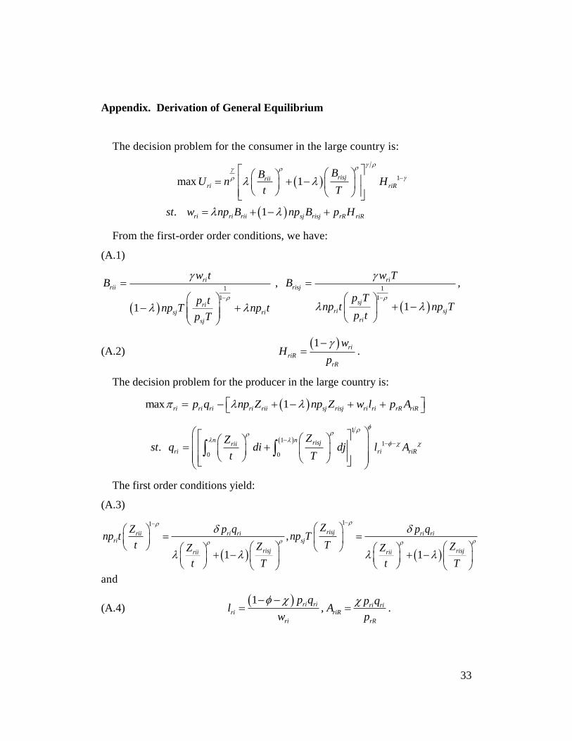
Appendix. Derivation of General Equilibrium

The decision problem for the consumer in the large country is:

1max 1

. 1

risjriiri riR

ri ri rii sj risj rR riR

BBU n H

t T

st w np B np B p H

From the first-order order conditions, we have:

(A.1)

1

1

1

ri

rii

ri

sj ri

sj

w tB

p tnp T np t

p T

,

1

1

1

ri

risj

sj

ri sj

ri

w TB

p Tnp t np T

p t

,

(A.2) 1 ri

riR

rR

wH

p

.

The decision problem for the producer in the large country is:

max 1ri ri ri ri rii sj risj ri ri rR riRp q np Z np Z w l p A

1

11

0 0.

n n risjrii

ri ri riR

ZZst q di dj l A

t T

The first order conditions yield:

(A.3)

11

,

1 1

risjrii ri ri ri riri sj

risj risjrii rii

ZZ p q p qnp t np T

t TZ ZZ Z

t T t T

and

(A.4) 1

,ri ri ri ri

ri riR

ri rR

p q p ql A

w p

.

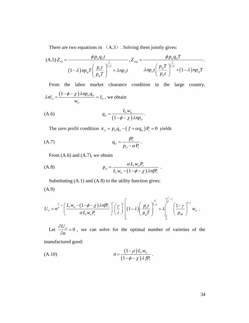
34

There are two equations in （A.3）. Solving them jointly gives:

(A.5)

1 1

1 1

,

11

ri ri ri ririi risj

sjriri sjsj ri

risj

p q t p q TZ Z

p Tp tnp t np Tnp T np t

p tp T

.

From the labor market clearance condition in the large country,

1 ri ri

ri r

ri

np qnl L

w

, we obtain

(A.6) 1

r riri

ri

L wq

np

.

The zero profit condition ri ri ri ri rp q f q P yields

(A.7) rri

ri r

fPq

p P

.

From (A.6) and (A.7), we obtain

(A.8) 1

r ri rri

r ri r

L w Pp

L w nfP

.

Substituting (A.1) and (A.8) to the utility function gives:

(A.9)

111 1

1r ri r ri

ri ri

r ri r sj rR

L w nfP p tU n w

L w P t p T p

.

Let 0riU

n

, we can solve for the optimal number of varieties of the

manufactured good:

(A.10)

1

1

r ri

r

L wn

fP

.

35

From (A.10), (A.8) and (A.7), we solve for the price and quantity produced in

the large country of the manufactured good i:

(A.11) rri

Pp

，

1ri

fq

.

From the land market clearance condition in the large country

r riR riR rL H nA R , we solve for the land rental in the large country:

(A.12) 11

r rirR

r

L wp

R

.

Substituting (A.4), (A.5), (A.10), (A.11), (A.12) into the production function,

we can obtain the following equation:

(A.13)

111 1 1

1 111

1 1

r rri r

r s

R Lw Pt

P f t PT

Following a similar procedure for the small country, we can obtain

(A.14)

1, ,

1 1 1

s sj ssj sj

s

L w P gn p q

gP

，

11

s sj

sR

s

L wp

R

and

(A.15)

1 1 11 11

11 1 1

sj s ss

s r

w R LP

P PT g

From (A.10) and (A.14), we have:

(A.16) 1 1 1

s sjr ri

r s

L wL w

fP gP

.

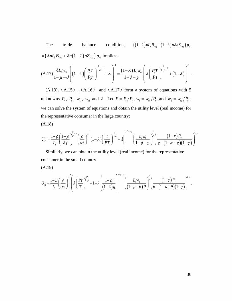
36

The trade balance condition, 1 1r risj risj sjnL B n nZ p

1s sjri sjri rinL B n nZ p implies:

(A.17)

1 11 1

1 11 11

1 11 1

s sj r ri sr

s r

L w L w PTPT

P Pt

.

(A.13),（A.15）,（A.16） and（A.17）form a system of equations with 5

unknowns rP , sP , riw , sjw and . Let s rP P P , 1 ri rw w P and 2 sj rw w P ,

we can solve the system of equations and obtain the utility level (real income) for

the representative consumer in the large country:

(A.18)

1

11

11 11

1 1 1

rrri

r

RL wtU

L f t PT

Similarly, we can obtain the utility level (real income) for the representative

consumer in the small country.

(A.19)

1

12

11 11

1 1 1 1

sssj

s

RL wPU

L T g P

.