Comments Welcome

The Term Structure of Country Risk and

Valuation in Emerging Markets *

Juan J. Cruces† Marcos Buscaglia†† Joaquín Alonso‡

First draft: Jan. 31, 2002

This draft: Aug. 12, 2002

Abstract

The prevailing valuation technique in Emerging Markets adds the country risk spread to the discount

rate in an ad-hoc manner. This practice does not account for the term structure of default risk. The

mismatch between the duration of the project being valued and the duration of the measure of country

risk used, such as J.P. Morgan’s EMBI, leads to an overvaluation (undervaluation) of long-term

projects when the term structure of default risk is upward (downward) sloping. Even if the term

structure of default risk were flat, this practice implies attenuating the covariance risk premium.

Using sovereign bond data from five Emerging Markets, we estimate a simple model that captures

most of the variation of expected collection at different horizons for a given country at one point in

time. We show the mispricing errors that are likely to be incurred in practice and how our model can

be used to avoid them.

JEL classification codes: G15, G31

Keywords : Emerging Economies, Cost of Capital, Default Risk

* We thank Javier García Sánchez, Andrew Powell, Ramiro Tosi and seminar participants at Univ. de San

Andrés, Univ. Torcuato Di Tella, IAE-Univ. Austral, Univ. of La Plata, Catholic Univ. of Argentina, CEMA,and the Latin American meetings of the Econometric Society (Sao Paulo, Brazil) for useful comments andGloria M. Kim from J.P. Morgan-Chase for kindly providing the panel of EMBI duration data. The mostcurrent version of this paper is posted at http://www.udesa.edu.ar/cruces/cc.

† Universidad de San Andrés, Argentina. E-mail address: cruces@udesa.edu.ar†† IAE School of Management and Business, Universidad Austral. Mariano Acosta s/n y Ruta Nac. 8, Casilla de

Correo 49, B1629WWA Pilar, Provincia de Buenos Aires, Argentina. Tel.: +54-2322-481069. E-mailaddress: mbuscaglia@iae.edu.ar. Corresponding author.

‡ Mercado Abierto, S.A., Buenos Aires, Argentina. E-mail address: joaquin@masa.com.ar.

1

I. Introduction

Investment projects in emerging markets are generally perceived as riskier than otherwise

similar projects in developed countries. The “additional risks” include currency

inconvertibility, civil unrest, institutional instability, expropriation, and widespread

corruption. Emerging markets (henceforth EM) are also more volatile than developed

economies: their business cycles are more intense, and inflation and currency risks are

higher.1

Several problems have restricted the use among practitioners of the Capital Asset Pricing

Model (CAPM) or its international version, the IAPM, to calculate the cost of capital of

projects in EM. First, there is no complete agreement about the degree of integration of EM

capital markets to the world market (see Errunza and Losq, 1985, and Bekaert et al., 2001).

Second, local returns are non-normal, show significant first-order autocorrelation (Bekaert et

al., 1998), and there are problems of liquidity and infrequent trading (Harvey, 1995). Finally,

as these additional risks are seldom covariance risks, the cost of capital that emerges from the

IAPM appears as “too low”.

Traditional finance theory would suggest dealing with idiosyncratic risks in the numerator

and handling covariance risks by adjusting the discount rate of a present value equation. But

given the practical difficulty of estimating truly expected cash flows and the lack of

consensus among academics on what the appropriate discount rate should be, the standard

approach is to use the most likely dividends in the numerator and hike the discount rate to

penalize for the additional risks of EM. Godfrey and Espinosa (1996), for instance, propose

to calculate the cost of capital in EM (k) by using

( ) ( )frECSfkE mUS

US

jjj −++=

σ

σ6.0 (1)

1 Neumeyer and Perri (2001) find that output in Argentina, Brazil, Korea, Mexico and Philippines is at least

twice as volatile as it is in Canada.

2

where f is the risk free rate, jCS is the credit spread between the yield of a U.S. dollar-

denominated EM sovereign bond of country j and the yield of a comparable U.S. bond, and

the term preceding the last parenthesis is an “adjusted beta”, that is equivalent to 60% of the

ratio of the volatility of the domestic market to that of the U.S. market.2 Although there are

different versions of this model (see Pereiro and Galli, 2000, Abuaf and Chu, 1994, and

Harvey, 2001), all of them add the country risk to the U.S. risk free rate in order to define the

EM´s “analog” of the U.S. risk free rate.

There are few systematic surveys of cost of capital estimation practices in EM, but those

available show that variants of this model are the most widely used among practitioners.

Keck et al. (1998) find in a survey of Chicago School of Business graduates that in

international valuations most respondents adjust discount rates for factors such as political,

sovereign, or currency risks. Pereiro and Galli (2000) show that the vast majority of

Argentine firms add the country risk to the U.S. risk free rate.3

Several objections have been raised in the literature to the addition of the country risk to the

discount rate. First, the model lacks any sound theoretical foundation (Harvey, 2001).

Second, in most versions of this model country risk is double counted, since part of the

variability in local market returns is correlated with country risk and this correlation is likely

to vary across countries (Estrada, 2000). Third, for global investors part of the country risk is

diversifiable, and hence it should not be included in the discount rate. Fourth, although this

model gives a unique discount rate for all projects, the “additional” risks inherent to EM do

not have a uniform impact on all firms and projects (Harvey, 2001). For example, the country

risk may be high because the market expects a sharp devaluation that would deteriorate the

public sector’s financial position. A devaluation, however, would benefit some sectors (e.g.,

exporters), and damage others (e.g., importers).

2 The 60% adjustment is due to the finding of Erb, Harvey and Viskanta (1995) that on average, about 40% of

the volatilities of emerging equity markets are explained by variations in credit quality. To avoid double-

counting credit risk, only the fraction of equity variation that is unaccounted for by variation in credit spreads

is taken into account --see Godfrey and Espinosa (1996) for details.

3 A number of important investment banks also add the country spread to the discount rate (Harvey, 2001).

3

In this paper we show that there is a very narrow set of circumstances under which this

approach delivers correct values and propose a simple and more general method that provides

more accurate values than the current practice.

First and foremost, we show that the mismatch between the duration of the project under

valuation and the duration of the most widely used measures of country risk leads to an

overvaluation (undervaluation) of long-term projects when the term structure of default risk is

upward (downward) sloping. The reverse is true for short-term projects. Second, we show

that even if each cash flow were discounted with CSj in (1) matching the duration of that

cash-flow, this would imply attenuating the covariance risk premium.4

The country risk measures most widely used are J.P. Morgan’s Emerging Market Bond Index

(EMBI), and its extensions EMBI+ and EMBI-Global (see Pereiro, 2001). Assuming zero

covariance risk, using these default risk measures in the discount rate to value long-term

projects would bear no additional problem to the ones mentioned above if the default risk

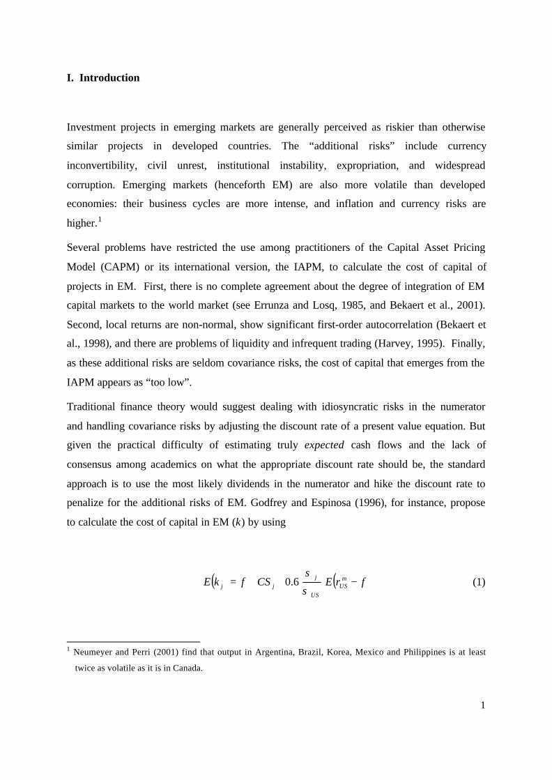
term structure were flat. But, in fact, this is not the case. In normal times, default risk spreads

are low at the short end of the curve and slope upward for longer durations. Often times,

however, the default risk term structure is downward sloping --as when the market expects a

default in the short run. Figure I.C. illustrates our first point: if, say, the project at hand had a

duration of four years and Argentina’s and Russia’s EMBI spreads had a duration of two

years each, valuation according to (1) would have overestimated the value of the Argentinean

relative to the Russian project.

4 To overcome some of the criticisms to using (1) Harvey (2001) proposes a model, based on Erb, Harvey and

Viskanta (1996), that relates expected returns to credit ratings according to ( ) ( )jj CCRaakE lnˆˆ 10 += ,

where CCRj is country j’s credit rating, as measured by Institutional Investor’s semiannual survey of bankers.

Our first critique also applies to this model, given that a single CCR is used to discount project cash flows of

different maturities, when the true credit risk varies by horizon. Moreover, the horizon for which credit ratings

are assessed is likely to vary across countries to match that of the loans extended to each nation by banks (see

Cruces, 2001, for details). Our second critique is harder to show based on Harvey’s proposal since he mixes

the covariance and institutional risks of EM in one CCR measure. Therefore the rest of the paper focuses on

equation (1).

4

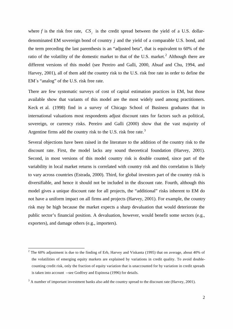
In addition, there is a high cross-country variability in the average duration of the EMBI-

Global country components (see Figure II).5 While the average duration for Bulgaria is lower

than one year, for Poland it is eight years. This variability undermines the significance of net

present value comparisons of otherwise similar projects in different countries, discounted in

each country with the EMBI Global as the country spread used in equation (1).

Using sovereign bond data from five Emerging Markets, we estimate a simple model that

captures most of the variation in the sequence of expected collection for a given country at

one point in time. This model can be used to solve the misvaluation problem.

The paper proceeds as follows. Section II presents the model, discusses the conditions under

which the current practice provides the right solution and obtains the correct valuation under

a more general set of circumstances. Section III describes the data and section IV presents the

estimation results. Section V concludes.

II. The Model

II.1. Bond Prices and Expected Collection

Let r0,t be the yield to maturity implicit in the price of a risky sovereign zero-coupon bond

denominated in U.S. dollars issued at time 0 and maturing at time t. Similarly, let f0,t be the

expected return of holding this bond during the same time interval. 6 In line with Claessens

and Pennacchi (1996) and Cumby and Pastine (2001) we assume that EM sovereign bonds

carry no systematic risk and so f is the risk free rate. Let Qt be the probability of full payment

5 Naturally, not all practitioners use the EMBI spread as a measure of country risk, although anecdotal evidence

suggests that it is the preferred one (see for instance Pereiro, 2001). The most important feature of the

literature and of investment bank brochures we have reviewed, however, is the use of one rate per country

regardless of the duration of the project under valuation. Some acknowledge the problem of cross-country

comparison and use bonds of similar maturities (but not duration) for all countries. Mariscal and Hargis

(1999), for instance, use 10-year Eurobonds, while Shores and Santos (2001) use 30-year bonds.

6 Both r0,t and f0,t are quoted on a per-period basis and we omit the j country subscript from now to avoid clutter.

5

on this bond, and tγ the recovery rate in the event of default. For a one-period bond issued at

time zero, these definitions imply,

( ) ( ) ( ) 1,01,011,01 1111 frQrQ t +=+−++ γ . (2)

Rearranging the left-hand side gives the expected collection per dollar due, P1,

( )1,0

1,0111 1

11

r

fQQP

++

=−+= γ . (3)

Similarly, if there is another bond issued at t=0 and maturing at t=2, we have

( ) ( )22,0

22,02 11 frP +=+ . (4)

So given a sequence of promised and expected yields for zero-coupon zero-beta bonds of

different maturities we can extract the sequence of expected collections for different horizons

implicit in bond prices. We call default spread the ratio )1/()1( ,0,0 tt fr ++ . From (3) and (4) it

is easy to see that if the default spread is constant for all t, then

tt PP 1= (5)

6

The case of constant default spreads corresponds to a risky yield curve whose slope is that of

the risk free yield curve times 11 P .7 As we argued in Section I, this case is a rare exception

in the data. Most of the time, EM default spreads vary with duration. To account for this, we

propose a reduced form model for expected collection over time that seems consistent with

the data,8

≥

==

2

1

1

1

tifP

tifPP

tt δµ . (6)

Note that this model reduces to (5) in the special case of constant default spreads

(i.e., 1== δµ ).

II.2. Implications on Valuation in EM

The volatile environments of EM aggravate the usual difficulties of forecasting dividends

many years into the future under different states of nature and their associated probabilities.

The standard response to this problem has been to work with the most likely dividends (or the

expected dividends under normal circumstances) in the numerator of a present value equation

and to add extra factors to the discount rate as in equation (1) to penalize for the upward bias

of the most likely dividends in estimating the true expected dividends (see Keck et al., 1998,

Pereiro and Galli, 2000, Abuaf and Chu, 1994, Godfrey and Espinosa, 1996). This can be

interpreted in terms of the typical “downward” risks of EM noted by Estrada (2000).

7 If default spreads are constant for all t, then from (3) and (5) ( )tt fPP

r ,011

,0 11

+−= . In this case, the slopes

of the two yield curves will be related by ( )tsttst ffP

rr ,0,01

,0,0

1−=− ++ . Note that when the risk free yield

curve is flat, the risky yield curve would also be flat.

8 See Merrick (2001) and Yawitz (1977) for alternative specifications.

7

Consider the case of a firm located in an EM whose expected dividends conditional on

normal circumstances are d̂$ (constant) per period forever.9 Let MPr βτ +,0 be the constant

per-period discount rate stemming from (1), where τ stands for the interest rate duration of

the bond portfolio used to measure the country risk, and MPβ is analogous to the last term

in (1).10 In this case, the common practice is to compute the value of the firm as

MPrd

MPrd

Vt

t ββ ττ +=

++= ∑

∞

= ,01 ,0

ˆ

)1(

ˆˆ . (7)

We call V̂ “miscalculated value”, for reasons that will become apparent below. Note that,

from (4),

ττ

ττ 1

,0,0

11

P

fr

+=+ , (8)

so that (7) is equivalent to

( )( ) τ

ττ

ττ

ττ

τττ

ττ

ββ11

,0

1

11

,0

1

1

ˆ

1

ˆˆ

PMPPf

dP

MPPf

dPV

tt

t

−++=

++= ∑

∞

=

. (9)

Therefore, the standard approach is tantamount to adjusting central scenario dividends by

direct compounding of the τ -th root of the expected collectionτ -periods hence, and using in

the denominator an expected return where the market premium is attenuated by ττ1P .

9 We use “most likely dividends,” “central scenario dividends,” and “expected dividends conditional on normal

circumstances” interchangeably.

10 Here τττ ,0,0,0 CSfr += in (1).

8

We argue that this is not the best way to convert central scenario dividends into expected

dividends, as it does not make an efficient use of the data available from bond markets. Our

proposed alternative consists in using the actual sequence of expected collections on

government bonds, Pt, as a proxy for the likelihood that central scenario dividends will be

realized in each period. The idea is that in the states of nature in which the government breaks

its promise to lenders it might also break its promise to foreign direct investors about

respecting property rights and it might impose similar losses on both types of investors.11

On the one hand, the government could be more likely to violate the rights of direct investors

than those of bondholders. Given that the secondary market for direct investment claims is

much less liquid than that for sovereign bonds, it is relatively more costly for direct investors

to get rid of their firms than it is for bondholders and the government may take advantage of

this fact.

On the other hand, direct investors are stakeholders in the local economy and have more

retaliatory power than bondholders. While both types of investors can threaten to curtail

future investment, direct investors can backfire immediately by laying off workers (so raising

civilian unrest), postponing the liquidation of foreign exchange earnings (so further reducing

the demand for local currency in times of runs on the currency), or delaying investments

currently underway, etc. So the government may actually be less hostile towards direct

investors.

We use the working assumption of equal expected collection of central scenario cash flows

for the bond and equity markets, implicitly assuming that these effects might cancel one

another out. Equation (9) shows that the standard practice tacitly makes a similar assumption,

though it uses an adjustment factor in the numerator, which -under our hypothesis- may be

inconsistent with the information provided by bond markets. Our proposal does not provide a

solution to the fact that expected collections may vary by sector of industry. Our contribution

is to compute the mispricing errors that arise from (9) when the term structure of default risk

is non flat and to provide a simple solution to adjust the valuation for any term structure of

11 There are many ways in which the government can violate the property rights of direct investors, for instance

by changing public utility rate regulations, by shifting tax rates, by inducing inflation when some prices are

fixed or by outright confiscation. This is the standard justification for the sovereign ceiling usually imposed

on corporate bond ratings in EM (see Durbin and Ng, 1999, for details).

9

expected collection. 12 Moreover, our proposal is immune from the attenuation of the

covariance risk premium noted in (9).

We can think that the amount of dividends received and the maintenance of the current

property rights are not independent events. Let ( )ldg DL , denote the joint probability density

function of these two random variables. While D is a continuous positive random variable, L

is discrete and equals 1 under normal circumstances and 0 when the government (at least

partially) violates property rights. Then, expected year-t dividends are

( ) ( )∑∫=

=

∞

=1

0 0

,l

lt

tDLtt ddldgdDE (10)

Given that the joint density is always equal to the product of the conditional and the marginal

densities, (10) can be rearranged as,

( ) ( ) ( ) ( ) ( )0|0Pr1|1Pr ==+=== ttttttt LDELLDELDE (11)

Note that td̂ is equal to ( )1| =tt LDE . If we associate ( )1Pr =tL with the probability of full

payment on sovereign debt in year t and assume that foreign director investors will be

confiscated a similar amount than bondholders in the event of default in that year, then we

can set ( ) tttt dLDE ˆ0| γ== . Plugging this in (11) gives,

( ) ( )[ ] ttttttt dPdQQDE ˆˆ1 =−+= γ (12)

Conditional on these assumptions, the “true value”, V, of the firm would be

∑∞

= +=

1 ,0 )1(

ˆ

tt

t

t

idP

V (13)

12 See Robichek and Myers (1966) and Chen (1967) for an old debate about the effects on discount rates of

alternative assumptions about the resolution of uncertainty over time.

10

where i0,t is the expected rate of return of investing in this firm, and the numerator gives the

expected dividend each period. In equation (13) i0,t does not include the sovereign spread and

we can easily assume that it is constant.13 In financially integrated markets where the CAPM

holds, i would approximately be equal to the risk-free rate plus the beta of the firm with

respect to the world portfolio times the world market portfolio premium.14 In segmented

markets, beta and the market premium would be measured locally.

Given the proposed model for Pt in (6), equation (13) can be solved as

−+++

++= δ

δ

βµ

β 1

21

1 11

ˆ

PMPfP

PMPf

dV (14)

and so the practitioner, by using (9) instead of (14) would be introducing a mispricing error

m, given by

VVV

m−

=

∧

(15)

We can analytically distinguish between two sources of this mispricing error. The first one

arises, as is the main argument in this paper, from the use of a constant country spread rate

(CSj) that is obtained from a bond portfolio with a duration different from that of the project

under valuation. To see that, let 0=β in equations (9) and (14). We can express them,

respectively, as

−++

+=

−+=

ττ

τττ

τττ

ττ

1

21

1

1

11

ˆ

1

ˆˆ

Pf

PP

fd

Pf

dPV (9a)

13 Note that MPfi tt β+= ,0,0 . In Section V we show that given that the term structure of the risk-free rate is

relatively flat, assuming ff t =,0 is not a likely source of error.

14 Plus a term that reflects a premium for real exchange rate risk. See Adler and Dumas (1983).

11

and

−++

+= δ

δµ

1

21

1 11

ˆ

PfP

Pf

dV (14a)

From (9a) and (14a), and assuming that τ is smaller than the duration of a perpetuity, it can

be easily shown that )1(1 <> δδ implies ).0(0 <> mm

Let

−+

++= δ

δµ

1

21

1,0 1)1(

PfP

Pfr v in (14a) (so that vrdV ,0ˆ= ) where v is the duration of

the perpetuity. From this and equation (7) in the special case of 0=β , the mispricing ratio

becomes

τ

τ

,0

,0,0

r

rr

VVV

m v −=

−=

∧

(15a)

The mispricing ratio has a straightforward interpretation. If the default spread is upward

sloping and τ is smaller than the duration of the project, v (so that τ,0,0 rr v > ), then the

standard practice overestimates the value of the project (m>0). This is because such method

uses in the numerator of (9) a direct compounding of an expected collection that is very high

for the short run, and that when compounded directly over time, gives values of expected

collections for long-run dividends that are too high relative to what is implicit in

contemporaneous long bond prices. Hence the overestimation.

It could be argued, then, that just by using the “right” credit spread in the denominator of

each term in (7) we would get a correct valuation. This indeed is not the case. Using the

“right” rate from the term structure of sovereign yields to discount central scenario dividends

gives a value of the firm equal to

12

∑∞

= ++=

1 ,0 )1(

ˆ'ˆ

tt

t MPrd

Vβ

(7a)

which, conditional on (6), can be written as

( ) ( )∑∞

= +++

++=

21

1

1

1

1

ˆ

1

ˆ'ˆ

tt

t

t

tMPPf

dP

MPPf

dPV

βµ

µβ δ

δ

. (7b)

Assume, for the sake of simplicity, that the default spread is constant (i.e., 1== δµ ). Then,

there is no source of confusion as to what country risk spread should be used. Specializing

(7b) and (14) for this case, we can appreciate the second type of mispricing error that the

current practice induces,

( )11

1

11

PMPPfPMP

m−++

−=

ββ

. (15b)

Note that given 11 <P , this mispricing will always be positive. So that even if the “right”

yields were extracted for each duration from the sovereign rate spot curve (or if the risky and

risk free yield curves were flat), the current practice implicitly attenuates the market risk

premium and introduces a second source of mispricing error in the valuation.

In section IV we use data from U.S. dollar-denominated EM bonds to estimate the stP and

equation (6), and illustrate the mispricing ratios that are likely to be observed for empirically

reasonable values of µ and δ .

III. Data

We collected effective annual ask yields and durations of non-guaranteed U.S. dollar-

denominated EM sovereign bonds (typically called “global bonds”). Data are from

13

Bloomberg for the last trading day of each month since September 1995 until December

2001. Also included are comparable U.S. Treasury yields, which are taken as the risk free

rate.

The sample was narrowed to those emerging countries which had data for more than one

bond at any point throughout the sample: Argentina, Brazil, Colombia, Ecuador, Mexico,

Poland, Russia, Thailand, Turkey, and Venezuela. Since we focus on yields spaced one-year

apart starting one year from the beginning of each period, we further narrowed the sample to

countries whose shorter traded bond had a duration smaller than 365 days for three months

that we considered representative of likely yield curve configurations: April 1997, January

2000 and August 2001. This restricted our sample to Argentina, Colombia, Mexico, Russia

and Turkey. 15 For those sample months for which the shortest bond had a duration greater

than one year, we estimated the one-year yield by linear extrapolation of the two nearest

bonds available.

Figure I reports the yield curves for the sample considered, which were constructed by linear

interpolation of the available data.16 The horizontal axis shows the duration of the respective

bonds measured in years. Very few of the bonds used are actually zero coupon. However, we

used the fact that for zero coupon bonds, duration and maturity are equal and that the main

determinant of yield for a given credit quality is duration. Therefore, we assumed that each

country had outstanding, at each month in the sample, a set of zero coupon bonds for

maturities at one year intervals into the future.17 The duration of the longest zero coupon

bond so constructed was smaller than that for the bond outstanding of highest duration. In

line with Claessens and Pennacchi (1996) and Cumby and Pastine (2001) we assumed that

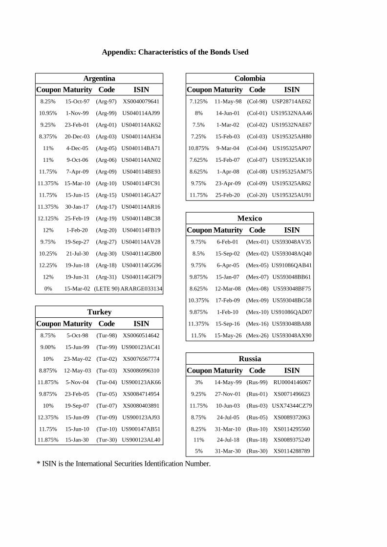
15 The appendix lists the characteristics of all the included bonds. The only bond that is partially guaranteed is

Russia-99, which had debentures as collateral. If the bond were stripped, the non-guaranteed part of the bond

should have a greater duration and a higher yield, so the April 1997 Russian yield curve would have had an

even greater downward slope than that reported in Figure I.C.

16 Plots of all available yields available are posted at http://www.udesa.edu.ar/cruces/cc/yield_curves.pdf.

17 Theoretically, it would be more appropriate to bootstrap the available bonds to generate a spot rate curve.

Unfortunately, given the paucity of EM bonds this procedure would hinge on imputing yields for horizons that

fall in between available bonds. We found more reasonable to pair each bond’s yield to maturity and duration

and to interpolate those points to generate an implicit zero-coupon bond yield curve.

14

these bonds had no systematic risk and so set their expected returns equal to the risk free rate

for each duration. With this information we used equation (3) to estimate the sequence of

expected collections for different horizons that are consistent with bond prices.

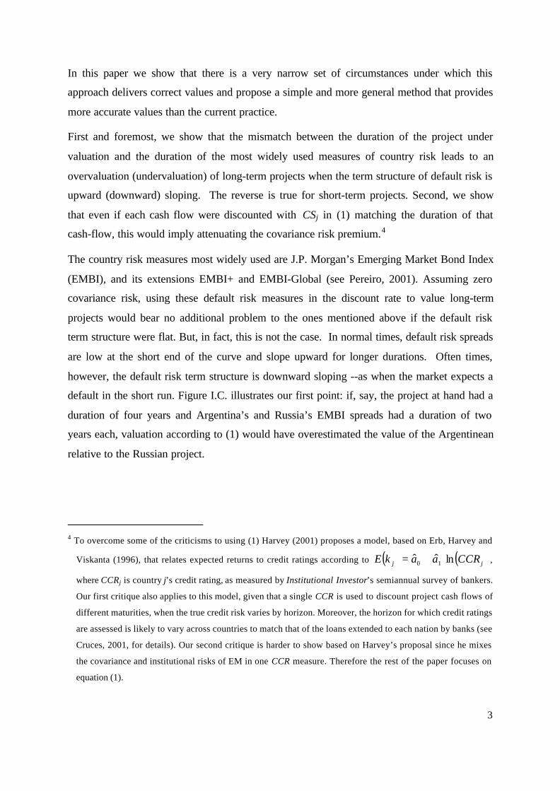
Figure III shows tP and ( )tP1 from this computation (it also shows the estimated tP from

model (3) which will be discussed below). It shows that while on some occasions tt PP 1≈ , it

is often the case that they differ substantially. For example, Figure I.A shows that Argentina

had a negatively sloping yield curve in August 2001. This translates in an expected collection

for year 10 implicit in bond prices of about 0.30, which is about twice the 0.16 that would

result from direct compounding of the first year expected collection. The reverse is true for

Colombia, which had a steep yield curve at that time.

IV. Estimation Results and their Implications on Valuation in EM

IV.1. Estimation of Expected Collection Model

With these data in hand, we estimated the empirical analog of equation (6),

( ) ( ) ( ) TtePtP tt ,...,2lnlnln 1 =++= δµ (16)

separately for each country and for each month, by OLS. The rationale behind separate

estimation is that the yield curves in Figure I change dramatically across time and countries

so that assuming a model with constant parameters would be inadequate. This shortcoming

could be avoided by the use of conditioning information so that µ and δ depend on lagged

instruments. While that is an interesting approach that we propose to explore in future

research, it would lead us into yield curve modeling, an issue beyond the scope of this paper.

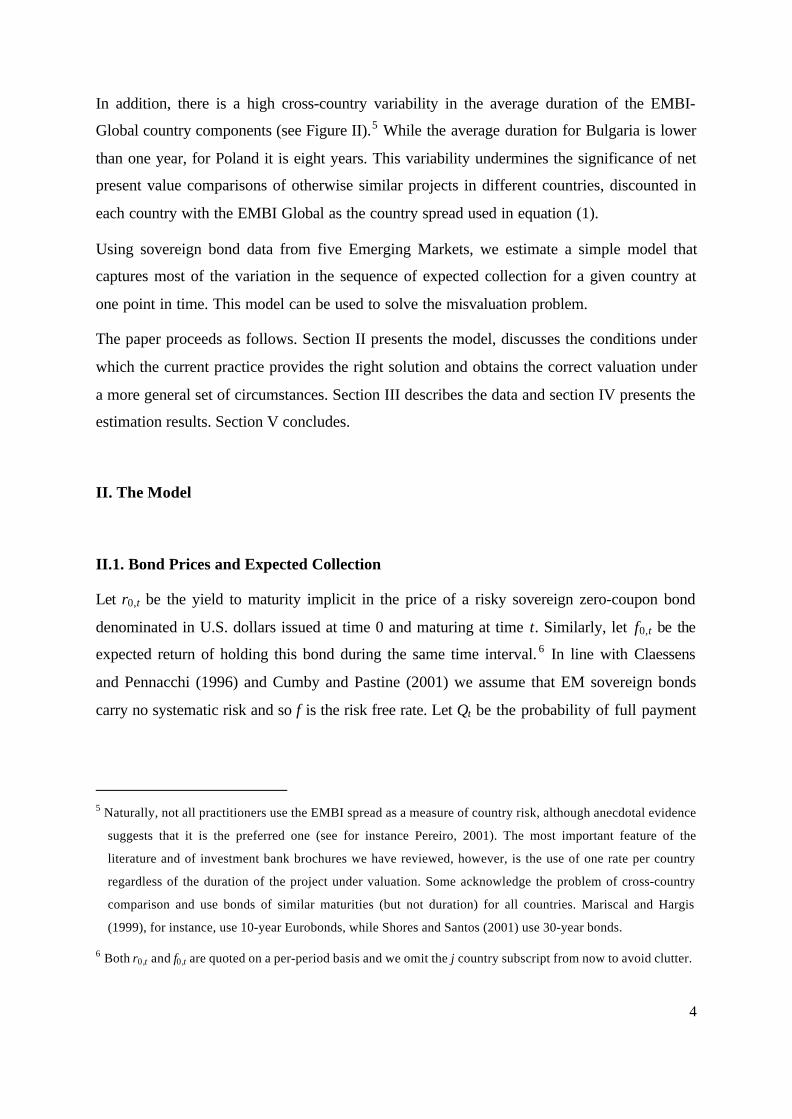
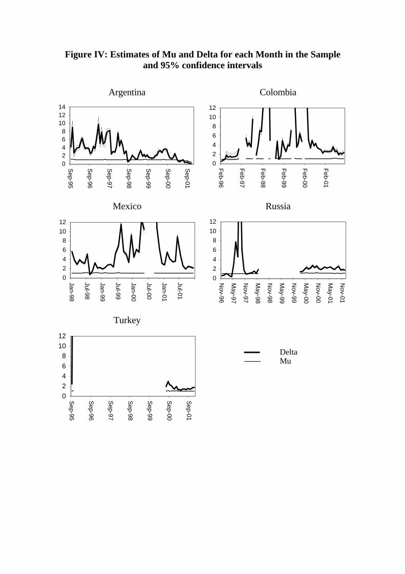
We estimated (16) for all months in the sample and report the key parameters. Figure IV

reports the estimated µ and δ for all months in the sample. It is apparent that most of the

action of the expected collection model is around the parameter δ , while µ is rather stable

15

around one over time for all countries. Most of the time δ is greater than one, corresponding

to an upward sloping default spread term-structure. Nevertheless, δ smaller than one are not

uncommon, as in Mexico and Argentina in mid-1998, Russia in early 1997, Colombia around

February 1996 and finally as Argentina approached the sovereign default of 2001.

Given the possible measurement error implicit in the extrapolation, we focus the subsequent

analysis on the results for three representative months at which the shortest traded bond had a

duration lower than one year. Table I reports the results for those three points along the

sample.18 All parameter estimates are statistically different from zero and the model fits well

the sequence of expected collection implicit in bond prices --a feature that is clearly

identifiable from the plots of fitted values in Figure III. Also, the estimated values agree with

the intuition that when sovereign spreads are upward sloping, sδ are greater than one, and

conversely when they are decreasing. It is noteworthy that, in spite of having few

observations for each regression, we can reject the null that the parameters are equal to one --

the maintained hypothesis in the standard practice reflected in equation (9) if the τ used is

one year. Sinceδ is the parameter that affects the expected collection as time passes, it is the

one that changes the most as the economic environment changes: from a minimum of about

0.4 as countries approach default (Argentina in August 2001 and Russia in April 1997) to

about 8 when the yield curve steeps up.

IV.2. Implications for Valuation in Emerging Markets

This section reports the main findings of the paper. We have argued above that from an

analytical point of view we can distinguish between two sources of mispricing error that the

prevailing valuation technique in EM induces. The first one arises from the addition of a

constant country risk spread to the cost of capital, while the second appears even if the

“right” country risk spread is added to the discount rate for each period. For each source we

present two alternative measures of the mispricing error, one based on the valuation of a

18 Given the deterministic time trend, the estimator of δ is superconsistent --it converges to its true value faster

than in a stationary regression. If the errors are Gaussian, then the usual OLS t-tests have exact small sample

t-distributions. Even if the innovations are not Gaussian, the t-tests are asymptotically valid (see Hamilton,

1994, p.460-462 for details).

16

perpetuity and the use of empirically reasonable parameter values, and the other based on the

valuation of projects of different durations and the use of observed interest rates in the

selected emerging markets.

Table II shows vr ,0 and the mispricing ratio m for 1=τ and 0=β as in (15a), for a range of

empirically reasonable parameter values. For µ =1 and δ =1.5, for instance, the constant

discount rate that would correctly value the project is 12 percent while the estimated value

assuming a flat term structure of default risk (i.e. a constant discount rate of 9 percent) would

be 30 percent higher than the true value.

When δ is less than one, the short-term sovereign spread is much higher than its long-term

counterpart and the estimated value can miss up to 35 percent of the true value. On the

contrary, when δ is larger than one, the estimated value under the current practice (using

1=τ ) can overestimate the true value of a project by a factor of about three or four.

For a given δ , �higher values of µ lower the estimated relative to the true value since a

higher µ raises expected dividends. Naturally, when the yield curve steeps up, the constant

discount rate that would make the value of the project from (7) equal to that of (14) is much

higher than the short-term rate.

As noted in Section I, however, instead of using a one-year sovereign spread , it is common

to use J.P. Morgan’s Emerging Bond Market Indices (EMBI) or some other single measure of

country risk in equation (1) . To have a clear sense of the magnitude of the mispricing error

that the current practice might have induced when the duration of the project differed from

that of the bond portfolio used to calculate the EMBI, we calculated it for each country and

each month in the sample for projects of various durations

For each country and each month in the sample we first calculated the hypothetical tP (t =

1,…, 10) that would have arisen from the estimated 1P , µ and δ and the use of equation (6).

From (8) and the term structure of the risk-free rate ( tf ,0 ), we obtained the hypothetical term

structure of the risky interest rate for each month. We also calculated the hypothetical risky

interest rate corresponding to the duration of the EMBI for each country and each month in

the sample ( τ,0r ). With these data in hand, we computed the mispricing error for zero-beta

17

projects of different durations as follows. For a project of duration s, the mispricing error is

given by

1

)1(1$

)1(1$

1ˆ

,0

,0 −

+

+=−=

ss

s

ss

r

r

VV

m τ (17)

Figure V reports the mispricing error, ms, for projects with durations of one year, five years,

and 10 years and shows some interesting results:19

- The mispricing error for projects of five years of duration is small in all countries

except Mexico, precisely because the duration of the EMBI has been close to five

years in those countries.

- The overvaluation of 10-year duration projects has typically been very high in all

countries throughout the sample: 9.5 % in Argentina –up to January 2001-, 11.1 % in

Colombia, 4.0 % in Mexico, 18.4 % in Russia, and 10.1 % in Turkey. The maximum

overvaluation of projects of this duration reached 25.2 % in Argentina (1999), 23.3 %

in Colombia (2001), 11.1 % in Mexico (1997), 105.9 % in Russia (1999), and 18.9 %

in Turkey (2001).

- In periods in which the term structure of the risky interest rate was inverted, as in

Argentina during 2001, the undervaluation of projects of 10 years of duration reached

50 %.

- Short-term projects were typically undervalued by around 3 %.

To have an idea of the relative magnitude of the mispricing error ms, note that most

practitioner-oriented books recommend the use of a 10-year Treasury bond rate as the risk

free rate in a U.S. valuation (e.g. Copeland et al., 2000). The mispricing error that would have

arisen from the use of this rate in the valuation of U.S. projects with a duration different from

that of the bond was in the range of –1 percent (for projects with a duration of four years) to

19 The mispricing errors for projects of other durations are available from the authors on request.

18

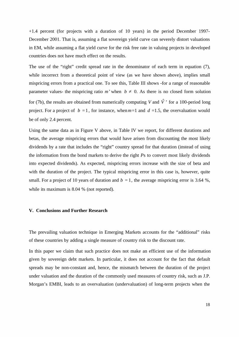
+1.4 percent (for projects with a duration of 10 years) in the period December 1997-

December 2001. That is, assuming a flat sovereign yield curve can severely distort valuations

in EM, while assuming a flat yield curve for the risk free rate in valuing projects in developed

countries does not have much effect on the results.

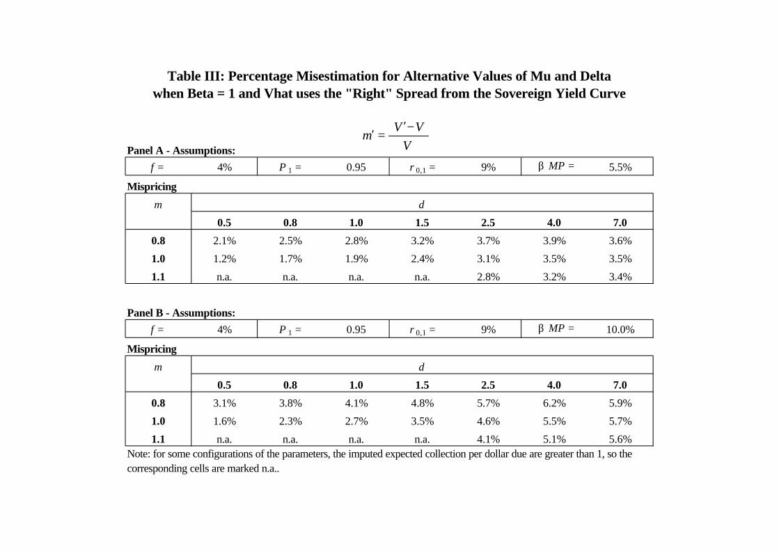
The use of the “right” credit spread rate in the denominator of each term in equation (7),

while incorrect from a theoretical point of view (as we have shown above), implies small

mispricing errors from a practical one. To see this, Table III shows -for a range of reasonable

parameter values- the mispricing ratio m’ when ≠β 0. As there is no closed form solution

for (7b), the results are obtained from numerically computing V and V̂ ’ for a 100-period long

project. For a project of 1=β , for instance, whenµ =1 and δ =1.5, the overvaluation would

be of only 2.4 percent.

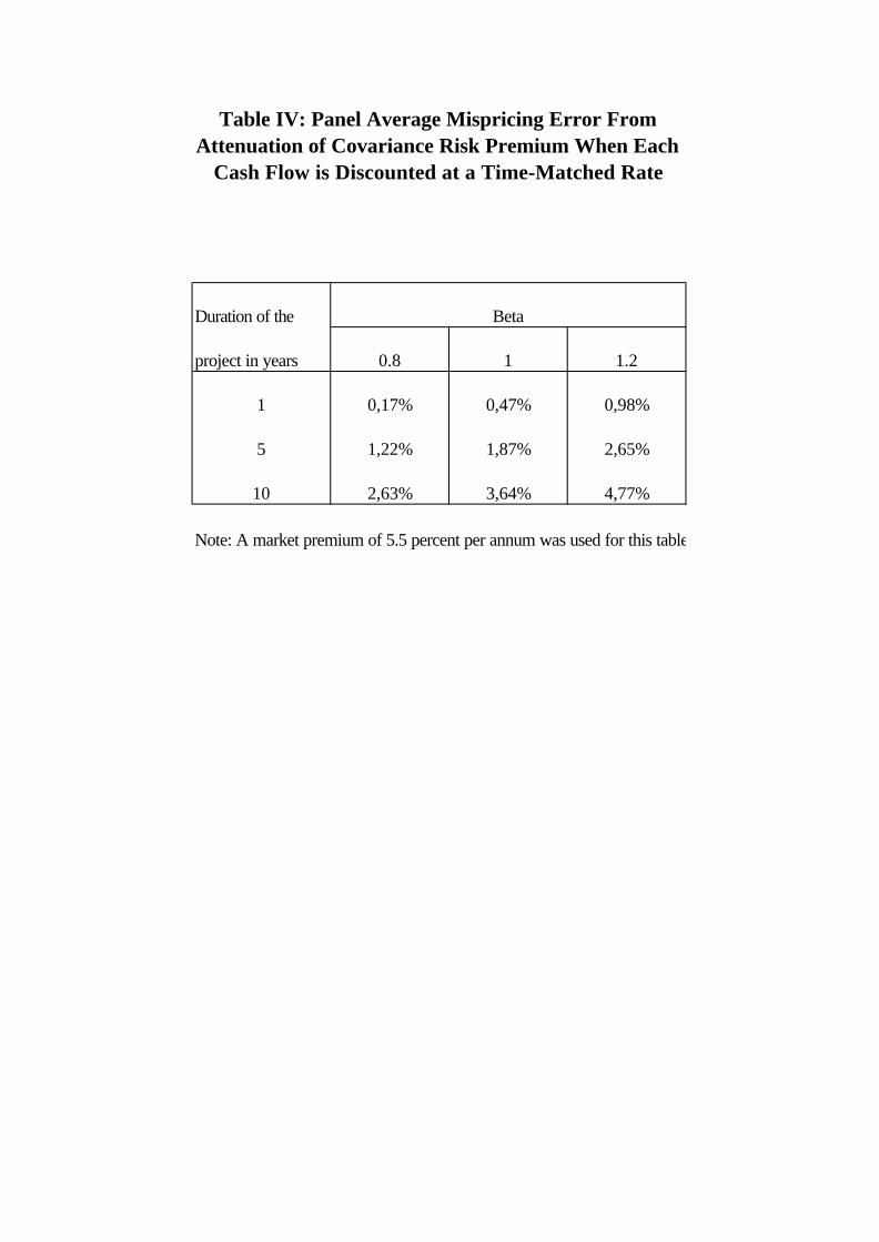
Using the same data as in Figure V above, in Table IV we report, for different durations and

betas, the average mispricing errors that would have arisen from discounting the most likely

dividends by a rate that includes the “right” country spread for that duration (instead of using

the information from the bond markets to derive the right Ps to convert most likely dividends

into expected dividends). As expected, mispricing errors increase with the size of beta and

with the duration of the project. The typical mispricing error in this case is, however, quite

small. For a project of 10 years of duration and 1=β , the average mispricing error is 3.64 %,

while its maximum is 8.04 % (not reported).

V. Conclusions and Further Research

The prevailing valuation technique in Emerging Markets accounts for the “additional” risks

of these countries by adding a single measure of country risk to the discount rate.

In this paper we claim that such practice does not make an efficient use of the information

given by sovereign debt markets. In particular, it does not account for the fact that default

spreads may be non-constant and, hence, the mismatch between the duration of the project

under valuation and the duration of the commonly used measures of country risk, such as J.P.

Morgan’s EMBI, leads to an overvaluation (undervaluation) of long-term projects when the

19

term structure of default risk is upward (downward) sloping. The reverse is true for short-

term projects.

We establish that such practice amounts to reducing central scenario dividends by a power of

the expected collection for a horizon equal to the duration of the bonds used to measure the

country spreads when 0=β . This would not be subject to additional criticisms to those

already raised in the literature if the default spreads were constant but it is problematic when

they are not. In normal times, however, default risk is low at the short end of the curve and

slopes upward for longer durations. Moreover, often times the default risk term structure is

downward sloping --as when the market expects a default in the short run.

We use data from five EM to estimate a simple model of the term structure of default risk and

derive its implications on valuation. We find that mispricing errors in the range of minus 30

to plus 400 percent can be made for reasonable parameter values under current practice

When 0>β , if each cash-flow is discounted at a duration-matched rate taken from the

sovereign spot rate curve, this amounts to attenuating the premium for covariance risk --

though the mistake incurred is not nearly as important.

To correct the mispricing, we propose a valuation procedure based on our model that treats

the institutional uncertainties of emerging markets separate from the covariance risk in a way

that is more amenable to financial theory than the standard practice and yet accounts for the

high idiosyncratic volatility of EM.

There are two directions for further research. First, it would be useful to generate expected

collections per dollar of central scenario cash flows that vary by industrial sector, since the

instability of EM has heterogeneous impact across sectors (Eaton and Gersovitz, 1984).

Second, by using conditioning information to model the term structure of default risk, one

could estimate how its shape responds to fundamentals. If yield spreads are upward sloping in

booms and downward sloping in recessions, and if a sizable share of the market is appraising

investments in the way that practitioner surveys indicate, then this would induce an extra pro-

cyclicality in private investment in EM.

Figure I. Yields on U.S. Dollar -Denominated Sovereign Bonds

Figure I.A. August 2001

0

5

10

15

20

25

30

1 2 3 4 5 6 7 8 9Duration in Years

Yie

ld (%

poi

nts)

Argentina

USA

Mexico

ColombiaRussia

Turkey

Figure I.B. January 2000

4

6

8

10

12

14

1 2 3 4 5 6 7 8 9Duration in Years

Yie

ld (%

poi

nts)

Argentina

USA

Mexico

Colombia

Figure I.C. April 1997

4

6

8

10

12

1 2 3 4 5 6 7 8Duration in Years

Yie

ld (%

poi

nts) Argentina

USA

Colombia

Russia

1. EMBI Global 5. Chile 9. Egypt 13. Mexico 17. Peru 21. Turkey2. Argentina 6. China 10. Hungary 14. Malaysia 18. Philippines 22. Uruguay3. Bulgaria 7. Colombia 11. Korea 15. Nigeria 19. Poland 23. Venezuela4. Brazil 8. Ecuador 12. Lebanon 16. Panama 20. Thailand 24. South Africa

Source: J.P. Morgan

Figure II: Interest Rate Duration of Selected EMBI-Global Country Components

D

FE

C

A BDecember 1997 - March 2002

-

1

2

3

4

5

6

7

Dec-97

Apr-98

Aug-98

Dec-98

Apr-99

Aug-99

Dec-99

Apr-00

Aug-00

Dec-00

Apr-01

Aug-01

Dec-01

Du

rati

on

in

Ye

ars 1

2

3

4

-

1

2

3

4

5

6

7

8

9

Dec-97

Mar-98

Jun-98

Sep-98

Dec-98

Mar-99

Jun-99

Sep-99

Dec-99

Mar-00

Jun-00

Sep-00

Dec-00

Mar-01

Jun-01

Sep-01

Dec-01

Mar-02

Du

rati

on

in

Ye

ars 5

6

7

8

-

1

2

3

4

5

6

7

Dec-97

Mar-98

Jun-98

Sep-98

Dec-98

Mar-99

Jun-99

Sep-99

Dec-99

Mar-00

Jun-00

Sep-00

Dec-00

Mar-01

Jun-01

Sep-01

Dec-01

Mar-02

Du

rati

on

in

Ye

ars

9

10

11

12

-

1

2

3

4

5

6

7

8

9

Dec-97

Mar-98

Jun-98

Sep-98

Dec-98

Mar-99

Jun-99

Sep-99

Dec-99

Mar-00

Jun-00

Sep-00

Dec-00

Mar-01

Jun-01

Sep-01

Dec-01

Mar-02

Du

rati

on

in

Ye

ars

13

14

15

16

-

1

2

3

4

5

6

7

8

9

Dec-97

Mar-98

Jun-98

Sep-98

Dec-98

Mar-99

Jun-99

Sep-99

Dec-99

Mar-00

Jun-00

Sep-00

Dec-00

Mar-01

Jun-01

Sep-01

Dec-01

Mar-02

Du

rati

on

in

Ye

ars

17

18

19

20

-

2

4

6

8

10

12

Dec-97

Mar-98

Jun-98

Sep-98

Dec-98

Mar-99

Jun-99

Sep-99

Dec-99

Mar-00

Jun-00

Sep-00

Dec-00

Mar-01

Jun-01

Sep-01

Dec-01

Mar-02

Du

rati

on

in

Ye

ars

21

22

23

24

August 2001

January 2000

April 1997

Fig. III: Expected Collection for Different Horizons (in Years)

Argentina

0.0

0.3

0.6

0.9

1 2 3 4 5 6 7 8 9 10 11

P(t)P(1)^tEstimated P(t)

Colombia

0.5

0.7

0.9

1.1

1 2 3 4 5 6 7 8

Argentina

0.6

0.7

0.8

0.9

1.0

1.1

1 2 3 4 5 6 7 8

Colombia

0.7

0.8

0.9

1.0

1.1

1 2 3 4 5 6

Mexico

0.7

0.8

0.9

1.0

1.1

1 2 3 4 5 6 7 8 9

Argentina

0.7

0.8

0.9

1.0

1.1

1 2 3 4 5 6 7 8

Colombia

0.8

0.9

1.0

1.1

1 2 3 4 5 6

Russia

0.80

0.86

0.92

0.98

1 2 3

Mexico

0.7

0.8

0.9

1.0

1.1

1 2 3 4 5 6 7 8 9

Russia

0.6

0.8

1.0

1 2 3 4 5 6 7

Turkey

0.5

0.7

0.9

1.1

1 2 3 4 5 6 7

Note: The source data for this figure are posted at http://www.udesa.edu.ar/cruces/cc/fig_3_source.xls.

Delta Mu

Turkey

Argentina Colombia

Figure IV: Estimates of Mu and Delta for each Month in the Sample

Mexico Russia

and 95% confidence intervals

02468

101214

Sep-95

Sep-96

Sep-97

Sep-98

Sep-99

Sep-00

Sep-01

0

2

4

6

8

10

12

Feb-96

Feb-97

Feb-98

Feb-99

Feb-00

Feb-01

0

2

4

6

8

10

12

Jan-98

Jul-98

Jan-99

Jul-99

Jan-00

Jul-00

Jan-01

Jul-01

0

2

4

6

8

10

12

Nov-96

May-97

Nov-97

May-98

Nov-98

May-99

Nov-99

May-00

Nov-00

May-01

Nov-01

0

2

4

6

8

10

12S

ep-95

Sep-96

Sep-97

Sep-98

Sep-99

Sep-00

Sep-01

Figure V: Mispricing Error when Using EMBI Spread to Discount Cash Flows of Projects of Different Durations

Argentina

-60%

-30%

0%

30%

60%

Dec-97 Dec-98 Dec-99 Dec-00 Dec-01

Colombia

-10%

0%

10%

20%

30%

Dec-97 Dec-98 Dec-99 Dec-00 Dec-01

Mexico

-6%-4%-2%0%2%4%6%8%

10%12%

Dec-97 Dec-98 Dec-99 Dec-00 Dec-01

Russia

-40%

0%

40%

80%

120%

Dec-97 Dec-98 Dec-99 Dec-00 Dec-01

Turkey

-10%

0%

10%

20%

30%

Dec-97 Dec-98 Dec-99 Dec-00 Dec-01

duration = 1 year

duration = 5 years

duration = 10 years

T -1 µ δ R 2

Argentina 10 0.75 0.40 0.98(0.022) (0.019)

Colombia 7 1.14 2.86 0.96(0.04) (0.249)

Mexico 8 1.06 2.55 0.99(0.007) (0.07)

Russia 6 1.06 2.31 0.99(0.005) (0.029)

Turkey 6 1.04 1.50 0.99(0.007) (0.024)

T -1 µ δ R 2

Argentina 7 1.04 2.03 0.97(0.028) (0.169)

Colombia 5 1.07 7.33 0.99(0.008) (0.256)

Mexico 8 1.06 4.53 0.99(0.008) (0.159)

T -1 µ δ R 2

Argentina 7 1.10 7.86 0.97(0.02) (0.628)

Colombia 5 1.04 5.45 0.98(0.007) (0.4)

Russia 2 0.95 0.37 .. .

Minimum 0.75 0.37Maximum 1.14 7.86

Table I: Estimates of Mu and Delta for Different Samples

Estimated by OLS. Standard errors in parentheses. For mu, the standard deviations estimated by the delta method are identical up to four digits with those resulting from assuming normal errors and using the exact lognormal variance. P -values from the t -distribution are smaller than one percent for all parameter estimates. No statistics are involved for Russia in April 1997 since only two usable observations are available in that case.

April 1997

January 2000

August 2001

( ) ( ) ( ) TtePtP tt ,...,2lnlnln 1 =++= δµ

Assumptions:

f = 4% P 1 = 0.95 r 0,1 = 9% β MP = 0 * 5.5% = 0

Mispricing

µ

0.5 0.8 1.0 1.5 2.5 4.0 7.0

0.8 -13% 8% 22% 58% 128% 232% 425%

1.0 -29% -12% 0% 30% 90% 182% 362%

1.1 -35% -19% -8% 19% 75% 162% 336%

µ

0.5 0.8 1.0 1.5 2.5 4.0 7.0

0.8 8% 10% 12% 15% 22% 31% 50%

1.0 7% 8% 9% 12% 18% 27% 44%

1.1 6% 8% 9% 11% 17% 25% 41%

δ

Table II: Percentage Misestimation for Alternative Values of Mu and Delta when Beta = 0

δ

vr ,0

1,0

1,0,0

rrr

VVV

m v −=−=

∧

Panel A - Assumptions:

f = 4% P 1 = 0.95 r 0,1 = 9% β MP = 5.5%

Mispricing

µ

0.5 0.8 1.0 1.5 2.5 4.0 7.0

0.8 2.1% 2.5% 2.8% 3.2% 3.7% 3.9% 3.6%

1.0 1.2% 1.7% 1.9% 2.4% 3.1% 3.5% 3.5%

1.1 n.a. n.a. n.a. n.a. 2.8% 3.2% 3.4%

Panel B - Assumptions:

f = 4% P 1 = 0.95 r 0,1 = 9% β MP = 10.0%

Mispricing

µ

0.5 0.8 1.0 1.5 2.5 4.0 7.0

0.8 3.1% 3.8% 4.1% 4.8% 5.7% 6.2% 5.9%

1.0 1.6% 2.3% 2.7% 3.5% 4.6% 5.5% 5.7%

1.1 n.a. n.a. n.a. n.a. 4.1% 5.1% 5.6%

Table III: Percentage Misestimation for Alternative Values of Mu and Deltawhen Beta = 1 and Vhat uses the "Right" Spread from the Sovereign Yield Curve

δ

δ

Note: for some configurations of the parameters, the imputed expected collection per dollar due are greater than 1, so the corresponding cells are marked n.a..

VVV

m−′

=′∧

Duration of the

project in years 0.8 1 1.2

1 0,17% 0,47% 0,98%

5 1,22% 1,87% 2,65%

10 2,63% 3,64% 4,77%

Note: A market premium of 5.5 percent per annum was used for this table.

Table IV: Panel Average Mispricing Error From Attenuation of Covariance Risk Premium When Each

Cash Flow is Discounted at a Time-Matched Rate

Beta

Coupon Maturity Code ISIN Coupon Maturity Code ISIN

8.25% 15-Oct-97 (Arg-97) XS0040079641 7.125% 11-May-98 (Col-98) USP28714AE62

10.95% 1-Nov-99 (Arg-99) US040114AJ99 8% 14-Jun-01 (Col-01) US19532NAA46

9.25% 23-Feb-01 (Arg-01) US040114AK62 7.5% 1-Mar-02 (Col-02) US19532NAE67

8.375% 20-Dec-03 (Arg-03) US040114AH34 7.25% 15-Feb-03 (Col-03) US195325AH80

11% 4-Dec-05 (Arg-05) US040114BA71 10.875% 9-Mar-04 (Col-04) US195325AP07

11% 9-Oct-06 (Arg-06) US040114AN02 7.625% 15-Feb-07 (Col-07) US195325AK10

11.75% 7-Apr-09 (Arg-09) US040114BE93 8.625% 1-Apr-08 (Col-08) US195325AM75

11.375% 15-Mar-10 (Arg-10) US040114FC91 9.75% 23-Apr-09 (Col-09) US195325AR62

11.75% 15-Jun-15 (Arg-15) US040114GA27 11.75% 25-Feb-20 (Col-20) US195325AU91

11.375% 30-Jan-17 (Arg-17) US040114AR16

12.125% 25-Feb-19 (Arg-19) US040114BC38

12% 1-Feb-20 (Arg-20) US040114FB19 Coupon Maturity Code ISIN

9.75% 19-Sep-27 (Arg-27) US040114AV28 9.75% 6-Feb-01 (Mex-01) US593048AV35

10.25% 21-Jul-30 (Arg-30) US040114GB00 8.5% 15-Sep-02 (Mex-02) US593048AQ40

12.25% 19-Jun-18 (Arg-18) US040114GG96 9.75% 6-Apr-05 (Mex-05) US91086QAB41

12% 19-Jun-31 (Arg-31) US040114GH79 9.875% 15-Jan-07 (Mex-07) US593048BB61

0% 15-Mar-02 (LETE 90) ARARGE033134 8.625% 12-Mar-08 (Mex-08) US593048BF75

10.375% 17-Feb-09 (Mex-09) US593048BG58

9.875% 1-Feb-10 (Mex-10) US91086QAD07

Coupon Maturity Code ISIN 11.375% 15-Sep-16 (Mex-16) US593048BA88

8.75% 5-Oct-98 (Tur-98) XS0060514642 11.5% 15-May-26 (Mex-26) US593048AX90

9.00% 15-Jun-99 (Tur-99) US900123AC41

10% 23-May-02 (Tur-02) XS0076567774

8.875% 12-May-03 (Tur-03) XS0086996310 Coupon Maturity Code ISIN

11.875% 5-Nov-04 (Tur-04) US900123AK66 3% 14-May-99 (Rus-99) RU0004146067

9.875% 23-Feb-05 (Tur-05) XS0084714954 9.25% 27-Nov-01 (Rus-01) XS0071496623

10% 19-Sep-07 (Tur-07) XS0080403891 11.75% 10-Jun-03 (Rus-03) USX74344CZ79

12.375% 15-Jun-09 (Tur-09) US900123AJ93 8.75% 24-Jul-05 (Rus-05) XS0089372063

11.75% 15-Jun-10 (Tur-10) US900147AB51 8.25% 31-Mar-10 (Rus-10) XS0114295560

11.875% 15-Jan-30 (Tur-30) US900123AL40 11% 24-Jul-18 (Rus-18) XS0089375249

5% 31-Mar-30 (Rus-30) XS0114288789

* ISIN is the International Securities Identification Number.

Turkey

Russia

Appendix: Characteristics of the Bonds Used

Argentina Colombia

Mexico

References

Abuaf, Niso, and Quyen Chu, 1994, The Executive´s Guide to International CapitalBudgeting: 1994 Update, Salomon Brothers.

Adler, Michael and Bernard Dumas, 1983, International Portfolio Choice and CorporationFinance: A Synthesis, Journal of Finance 38, 925-984.

Bekaert, Geert, Campbell R. Harvey, and Robin Lumsdaine, 2001, Dating the Integration ofWorld Equity Markets, Working paper, Duke University.

Bekaert, Geert, Claude Erb, Campbell R. Harvey and Tadas Viskanta, 1998, DistributionalCharacteristics of Emerging Markets Returns and Asset Allocation, Journal of PortfolioManagement, Winter, 102-116.

Chen, Houng-Yhi, 1967, Valuation under Uncertainty, Journal of Financial and QuantitativeAnalysis 2, 313-325.

Claessens, Stijn and George Pennacchi, 1996, Estimating the Likelihood of Mexican Defaultfrom the Market Prices of Brady Bonds, Journal of Financial and Quantitative Analysis31, 109-126.

Copeland, Tom, Tim Koller, and Jack Murrin, 2000, Valuation: Measuring and Managingthe Value of Companies, 3rd ed. (John Wiley and Sons, New York).

Cruces, Juan J., 2001, Statistical Properties of Sovereign Credit Ratings, Working paper,University of Washington.

Cumby, Robert E., and Tuvana Pastine, 2001, Emerging Market Debt: Measuring CreditQuality and Examining Relative Pricing, Journal of International Money and Finance 20,591-609.

Durbin, Erik, and David Tat-Chee Ng, 1999, Uncovering Country Risk in Emerging MarketBond Prices, International Finance Discussion Papers 1999-639.

Eaton, Jonathan and Mark Gersovitz, 1984, A Theory of Expropriation and Deviations FromPerfect Capital Mobility, Economic Journal 94, 16-40.

Erb, Claude, Campbell R. Harvey and Tadas Viskanta, 1995, Country Risk and Global EquitySelection, Journal of Portfolio Management, Winter, 74-83.

Erb, Claude, Campbell R. Harvey and Tadas Viskanta, 1996, Expected Returns and Volatilityin 135 Countries, Journal of Portfolio Management, Spring, 46-58.

Errunza, Vihang and Etienne Losq, 1985, International Asset Pricing under MildSegmentation: Theory and Test, Journal of Finance 40, 105-124.

Estrada, Javier, 2000, The Cost of Equity in Emerging Markets: A Downside Risk Approach,Emerging Markets Quarterly 4, 19-30.

Godfrey, Stephen and Ramón Espinosa, 1996, A Practical Approach To Calculating Costs ofEquity for Investments in Emerging Markets, Journal of Applied Corporate Finance 9,80-89.

Hamilton, James D., 1994, Time Series Analysis (Princeton University Press, Princeton, NJ).

Harvey, Campbell R., 1995, Predictable Risk and Returns in Emerging Markets, Review ofFinancial Studies 8, 773-816.

Harvey, Campbell R., 2001, The International Cost of Capital and Risk Calculator (ICCRC),Working paper, Duke University.

J.P. Morgan, Emerging Markets Bond Index Monitor, various issues.

Keck, Tom, Eric Levengood, and Al Longfield, 1998, Using Discounted Cash Flow Analysisin an International Setting: A Survey of Issues in Modeling the Cost of Capital, Journal ofApplied Corporate Finance 11, 82-99.

Mariscal, Jorge, and Kent Hargis, 1999, A Long-Term Perspective on Short-Term Risk,Global Emerging Markets, Goldman, Sachs & Co.

Merrick, John J., Jr., 2001, Crisis Dynamics of Implied Default Recovery Ratios: Evidencefrom Russia and Argentina, Journal of Banking and Finance 25, 1921-1939.

Neumeyer, Pablo Andrés and Fabrizio Perri, 2001, Business Cycles in Emerging Economies:The Role of Interest Rates, Working paper, Universidad Torcuato Di Tella.

Pereiro, Luis, 2001, The Valuation of Closely-Held Companies in Latin America, EmergingMarkets Review 2, 330-370.

Pereiro, Luis and María Galli, 2000, La Determinación del Costo de Capital en la Valuaciónde Empresas de Capital Cerrado: una Guía Práctica, Working paper, Centro deInvestigación en Finanzas, Universidad Torcuato Di Tella.

Robichek, Alexander and Stewart Myers, 1966, Conceptual Problems in the Use of Risk-Adjusted Discount Rates, Journal of Finance 21, 727-730.

Shores, Andrew, and Gustavo Santos, 2001, Strategy: Revision of Discount Rates, CreditSuisse First Boston, September.

Yawitz, Jess, 1977, An Analitical Model of Interest Rate Differentials and Different DefaultRecoveries, Journal of Financial and Quantitative Analysis , 481-490.