“Counting Your Customers” the Easy Way:An Alternative to the Pareto/NBD Model

Peter S. FaderBruce G. S. Hardie

Ka Lok Lee1

August 2003

1Peter S. Fader is the Frances and Pei-Yuan Chia Professor of Marketing at the Wharton School of theUniversity of Pennsylvania (address: 749 Huntsman Hall, 3730 Walnut Street, Philadelphia, PA 19104-6340; phone: 215.898.1132; email: faderp@wharton.upenn.edu; web: www.petefader.com). Bruce G. S.Hardie is Associate Professor of Marketing, London Business School (email: bhardie@london.edu;web: www.brucehardie.com). Ka Lok Lee is a graduate of the Wharton School of the University ofPennsylvania. The second author acknowledges the support of ESRC grant R000223742 and the LondonBusiness School Centre for Marketing

Abstract

“Counting Your Customers” the Easy Way:An Alternative to the Pareto/NBD Model

Today’s researchers are very interested in predicting the future purchasing patterns of theircustomers, which can then serve as an input into “lifetime value” calculations. Among themodels that provide such capabilities, the Pareto/NBD “Counting Your Customers” frameworkproposed by Schmittlein, Morrison, and Colombo (1987) is highly regarded. But despite therespect it has earned, it has proven to be a difficult model to implement, particularly becauseof computational challenges required to perform parameter estimation.

We develop a new model, the beta-geometric/NBD (BG/NBD), which represents a slightvariation in the behavioral “story” associated with the Pareto/NBD, but it is vastly easier toimplement. We show, for instance, how its parameters can be obtained quite easily in MicrosoftExcel. The two models yield very similar results, leading us to suggest that the BG/NBD couldbe viewed as an attractive alternative to the Pareto/NBD in any empirical application.

An important secondary objective of this paper is to convey the types of performance mea-sures and managerial diagnostics that should be regularly constructed and examined when de-veloping models for customer base analysis, whether or not models such as the BG/NBD orPareto/NBD are being utilized.

Keywords: Customer Base Analysis, Repeat Buying, Pareto/NBD, Probability Models,Forecasting, Lifetime Value

1 Introduction

Faced with a database containing information on the frequency and timing of transactions for

a list of past customers, it is natural to try to make forecasts about future purchasing patterns.

These projections often range from aggregate sales trajectories (e.g., for the next 52 weeks),

to individual-level conditional expectations (i.e., the best guess about a particular customer’s

future purchasing, given information about his past behavior). Many other related issues may

arise from a customer-level database, but these are typical of the questions that a manager

should initially try to address. This is particularly true for any firm with serious interest in

tracking and managing “customer lifetime value” (CLV) on a systematic basis. There is a great

deal of interest, among marketing practitioners and academics alike, in developing models to

accomplish these tasks.

One of the first models to explicitly address these issues is the Pareto/NBD “Counting Your

Customers” framework originally proposed by Schmittlein, Morrison, and Colombo (1987), here-

after SMC. This model was developed to describe repeat-buying behavior in a setting where cus-

tomers buy at a steady rate (albeit in a stochastic manner) for a period of time, and then become

inactive. More specifically, time to “dropout” is modelled using the Pareto (exponential-gamma

mixture) timing model; but while the customer is still active/alive, his repeat-buying behavior

is modelled using the negative binomial (Poisson-gamma) counting model. The Pareto/NBD is

a powerful model for customer base analysis, but its empirical application can be challenging,

especially in terms of parameter estimation.

Perhaps because of these operational difficulties, relatively few researchers actively followed

up on the SMC paper soon after it was published (as judged by citation counts). But it has

received a steadily increasing amount of attention in recent years as many researchers and

managers have become concerned about issues such as customer churn, attrition, retention, and

CLV. While a number of researchers (e.g., Balasubramanian et al. 1998; Jain and Singh 2002;

Mulhern 1999; Niraj et al. 2001) refer to the applicability and usefulness of the Pareto/NBD,

only a small handful claim to have actually implemented it. Nevertheless, some of these papers

(e.g., Reinartz and Kumar 2000; Schmittlein and Peterson 1994) have, in turn, become quite

popular and widely cited themselves.

1

The primary objective of this paper is to develop a new model, the beta-geometric/NBD

(BG/NBD), which represents a slight variation in the behavioral “story” that lies at the heart

of SMC’s original work, but it is vastly easier to implement. We show, for instance, how its

parameters can be obtained quite easily in Microsoft Excel, with no appreciable loss in the

model’s ability to fit or predict customer purchasing patterns. We develop the BG/NBD model

from first principles, and present the expressions required for making individual-level statements

about future buying behavior. We also provide an illustrative empirical application of the model,

comparing and contrasting its performance to that of the Pareto/NBD. The two models yield

very similar results, leading us to suggest that the BG/NBD should be viewed as an attractive

alternative to the Pareto/NBD in any empirical application.

An important secondary objective of this paper is to convey the types of performance mea-

sures and managerial diagnostics that should be regularly constructed and examined when de-

veloping models for customer base analysis, whether or not models such as the BG/NBD or

Pareto/NBD are being utilized.

Before developing the BG/NBD model, we briefly review the Pareto/NBD model (Section 2).

In Section 3 we outline the assumptions of the BG/NBD model, deriving the key expressions at

the individual-level, and for a randomly-chosen individual, in Sections 4 and 5 respectively. This

is followed by the aforementioned empirical analysis. We conclude with a discussion of several

issues that arise from this work.

2 The Pareto/NBD Model

The Pareto/NBD model is based on five assumptions:

i. While active, the number of transactions made by a customer in a time period of length t

is distributed Poisson with transaction rate λ.

ii. Heterogeneity in transaction rates across customers follows a gamma distribution with

shape parameter r and scale parameter α.

iii. Each customer has an unobserved “lifetime” of length τ . This point at which the customer

becomes inactive is distributed exponential with dropout rate µ.

2

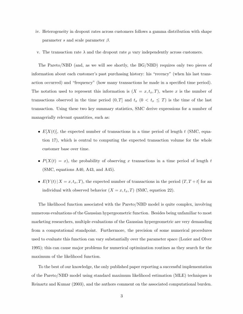
iv. Heterogeneity in dropout rates across customers follows a gamma distribution with shape

parameter s and scale parameter β.

v. The transaction rate λ and the dropout rate µ vary independently across customers.

The Pareto/NBD (and, as we will see shortly, the BG/NBD) requires only two pieces of

information about each customer’s past purchasing history: his “recency” (when his last trans-

action occurred) and “frequency” (how many transactions he made in a specified time period).

The notation used to represent this information is (X = x, tx, T ), where x is the number of

transactions observed in the time period (0, T ] and tx (0 < tx ≤ T ) is the time of the last

transaction. Using these two key summary statistics, SMC derive expressions for a number of

managerially relevant quantities, such as:

• E[X(t)], the expected number of transactions in a time period of length t (SMC, equa-

tion 17), which is central to computing the expected transaction volume for the whole

customer base over time.

• P (X(t) = x), the probability of observing x transactions in a time period of length t

(SMC, equations A40, A43, and A45).

• E(Y (t) |X = x, tx, T ), the expected number of transactions in the period (T, T + t] for an

individual with observed behavior (X = x, tx, T ) (SMC, equation 22).

The likelihood function associated with the Pareto/NBD model is quite complex, involving

numerous evaluations of the Gaussian hypergeometric function. Besides being unfamiliar to most

marketing researchers, multiple evaluations of the Gaussian hypergeometric are very demanding

from a computational standpoint. Furthermore, the precision of some numerical procedures

used to evaluate this function can vary substantially over the parameter space (Lozier and Olver

1995); this can cause major problems for numerical optimization routines as they search for the

maximum of the likelihood function.

To the best of our knowledge, the only published paper reporting a successful implementation

of the Pareto/NBD model using standard maximum likelihood estimation (MLE) techniques is

Reinartz and Kumar (2003), and the authors comment on the associated computational burden.

3

As an alternative to MLE, SMC proposed a three-step method-of-moments estimation procedure,

which was further refined by Schmittlein and Peterson (1994). While simpler than MLE, the

proposed algorithm is still not easy to implement; furthermore, it does not have the desirable

statistical properties commonly associated with MLE. In contrast, the BG/NBD model, to be

introduced in the next section, can be implemented very quickly and efficiently via MLE, and

its parameter estimation does not require any specialized software or the evaluation of any

unconventional mathematical functions.

3 BG/NBD Assumptions

Most aspects of the BG/NBD model directly mirror those of the Pareto/NBD. The only differ-

ence lies in the story being told about how/when customers become inactive. The Pareto timing

model assumes that dropout can occur at any point in time, independent of the occurrence of

actual purchases. If we assume instead that dropout occurs immediately after a purchase, we

can model this process using the beta-geometric (BG) model.

More formally, the BG/NBD model is based on the following five assumptions:

i. While active, the number of transactions made by a customer follows a Poisson process

with transaction rate λ. This is equivalent to assuming that the time between transactions

is distributed exponential with transaction rate λ, i.e.,

f(tj | tj−1;λ) = λe−λ(tj−tj−1) , tj > tj−1 ≥ 0 . (1)

ii. Heterogeneity in λ follows a gamma distribution with pdf

f(λ | r, α) = αrλr−1e−λα

Γ(r), λ > 0 . (2)

iii. After any transaction, a customer becomes inactive with probability p. Therefore the

point at which the customer “drops out” is distributed across transactions according to a

(shifted) geometric distribution with pmf

4

P (inactive immediately after jth transaction) = p(1 − p)j−1 , j = 1, 2, 3, . . . . (3)

iv. Heterogeneity in p follows a beta distribution with pdf

f(p | a, b) =pa−1(1 − p)b−1

B(a, b), 0 ≤ p ≤ 1 . (4)

where B(a, b) is the beta function, which can be expressed in terms of gamma functions:

B(a, b) = Γ(a)Γ(b)/Γ(a + b).

v. The transaction rate λ and the dropout probability p vary independently across customers.

4 Model Development at the Individual Level

4.1 Derivation of the Likelihood Function

Consider a customer who had x transactions in the period (0, T ] with the transactions occurring

at t1, t2, . . . , tx:

✲· · · · · ·0 T

×t1

×t2

×tx

We derive the individual-level likelihood function in the following manner:

• the likelihood of the first transaction occurring at t1 is a standard exponential likelihood

component, which equals λe−λt1 .

• the likelihood of the second transaction occurring at t2 is the probability of remaining active

at t1 times the standard exponential likelihood component, which equals (1−p)λe−λ(t2−t1).

. . .

• the likelihood of the xth transaction occurring at tx is the probability of remaining ac-

tive at tx−1 times the standard exponential likelihood component, which equals (1 −p)λe−λ(tx−tx−1).

5

• the likelihood of observing zero purchases in (tx, T ] is the probability the customer became

inactive at tx, plus the probability he remained active but made no purchases in this

interval, which equals p + (1 − p)e−λ(T−tx).

Therefore,

L(λ, p | t1, t2, . . . , tx, T ) = λe−λt1(1 − p)λe−λ(t2−t1) · · · (1 − p)λe−λ(tx−tx−1){p + (1 − p)e−λ(T−tx)}

= p(1 − p)x−1λxe−λtx + (1 − p)xλxe−λT

As pointed out earlier for the Pareto/NBD, note that information on the timing of the x trans-

actions is not required; a sufficient summary of the customer’s purchase history is (X = x, tx, T ).

Similar to SMC, we assume that all customers are active at the beginning of the observation

period, therefore the likelihood function for a customer making 0 purchases in the interval (0, T ]

is the standard exponential survival function:

L(λ |X = 0, T ) = e−λT

Thus we can write the individual-level likelihood function as

L(λ, p |X = x, T ) = (1 − p)xλxe−λT + δx>0 p(1 − p)x−1λxe−λtx (5)

where δx>0 = 1 if x > 0, 0 otherwise.

4.2 Derivation of P (X(t) = x)

Let the random variable X(t) denote the number of transactions occurring in a time period of

length t (with a time origin of 0). To derive an expression for the P (X(t) = x), we recall the

fundamental relationship between inter-event times and the number of events,

X(t) ≥ x ⇔ Tx ≤ t

6

where Tx is the random variable denoting the time of the xth transaction. Given our assumption

regarding the nature of the dropout process,

P (X(t) = x) = P (active after xth purchase) · P (Tx ≤ t and Tx+1 > t)

+ δx>0 · P (becomes inactive after xth purchase) · P (Tx ≤ t)

Given the assumption that the time between transactions is characterized by the exponential

distribution, P (Tx ≤ t and Tx+1 > t) is simply the Poisson probability that X(t) = x, and

P (Tx ≤ t) is the Erlang-x cdf. Therefore

P (X(t) = x|λ, p) = (1 − p)x(λt)xe−λt

x!+ δx>0 p(1 − p)x−1

[1 − e−λt

x−1∑j=0

(λt)j

j!

](6)

4.3 Derivation of E[X(t)]

Given that the number of transactions follows a Poisson process, E[X(t)] is simply λt if the

customer is active at t. For a customer who becomes inactive at τ ≤ t, the expected number of

transactions in the period (0, τ ] is λτ .

But what is the likelihood that a customer becomes inactive at τ? Conditional on λ and p,

P (τ > t) = P (active at t |λ, p) =∞∑

j=0

(1 − p)j(λt)je−λt

j!

= e−λpt

This implies that the pdf of the dropout time is given by

g(τ |λ, p) = λpe−λpτ

(Note that this takes on an exponential form. But it features an explicit association with the

transaction rate λ, in contrast with the Pareto/NBD, which has an exponential dropout process

that is independent of the transaction rate.) It follows that the expected number of transactions

in a time period of length t is given by

7

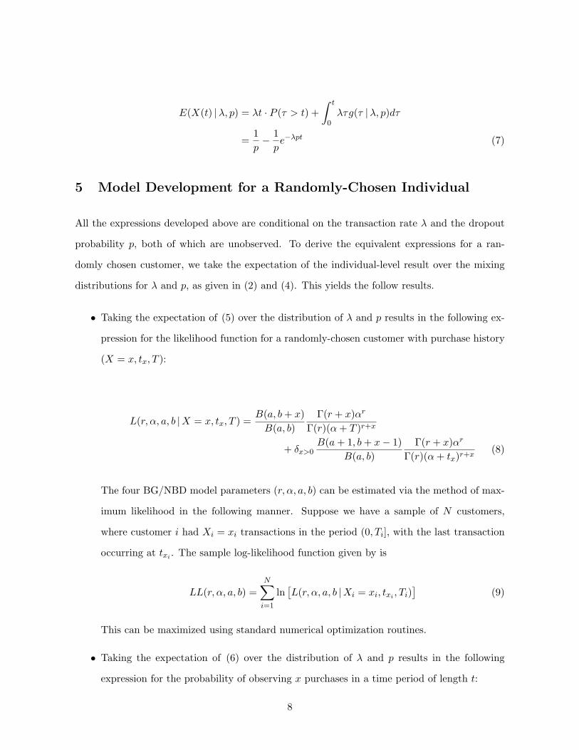
E(X(t) |λ, p) = λt · P (τ > t) +∫ t

0λτg(τ |λ, p)dτ

=1p

− 1pe−λpt (7)

5 Model Development for a Randomly-Chosen Individual

All the expressions developed above are conditional on the transaction rate λ and the dropout

probability p, both of which are unobserved. To derive the equivalent expressions for a ran-

domly chosen customer, we take the expectation of the individual-level result over the mixing

distributions for λ and p, as given in (2) and (4). This yields the follow results.

• Taking the expectation of (5) over the distribution of λ and p results in the following ex-

pression for the likelihood function for a randomly-chosen customer with purchase history

(X = x, tx, T ):

L(r, α, a, b |X = x, tx, T ) =B(a, b + x)

B(a, b)Γ(r + x)αr

Γ(r)(α + T )r+x

+ δx>0B(a + 1, b + x − 1)

B(a, b)Γ(r + x)αr

Γ(r)(α + tx)r+x(8)

The four BG/NBD model parameters (r, α, a, b) can be estimated via the method of max-

imum likelihood in the following manner. Suppose we have a sample of N customers,

where customer i had Xi = xi transactions in the period (0, Ti], with the last transaction

occurring at txi . The sample log-likelihood function given by is

LL(r, α, a, b) =N∑

i=1

ln[L(r, α, a, b |Xi = xi, txi , Ti)

](9)

This can be maximized using standard numerical optimization routines.

• Taking the expectation of (6) over the distribution of λ and p results in the following

expression for the probability of observing x purchases in a time period of length t:

8

P (X(t) =x|r, α, a, b) =B(a, b + x)

B(a, b)Γ(r + x)Γ(r)x!

(α

α + t

)r( t

α + t

)x

+ δx>0B(a + 1, b + x − 1)

B(a, b)

[1 −

(α

α + t

)r{ x−1∑j=0

(Γ(r + j)Γ(r)j!

(t

α + t

)j}](10)

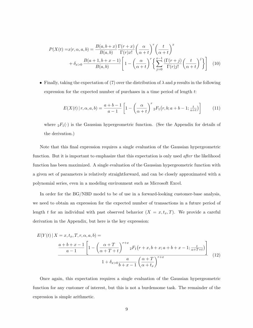
• Finally, taking the expectation of (7) over the distribution of λ and p results in the following

expression for the expected number of purchases in a time period of length t:

E(X(t) | r, α, a, b) =a + b − 1

a − 1

[1 −

(α

α + t

)r

2F1(r, b; a + b − 1; t

α+t

)](11)

where 2F1(·) is the Gaussian hypergeometric function. (See the Appendix for details of

the derivation.)

Note that this final expression requires a single evaluation of the Gaussian hypergeometric

function. But it is important to emphasize that this expectation is only used after the likelihood

function has been maximized. A single evaluation of the Gaussian hypergeometric function with

a given set of parameters is relatively straightforward, and can be closely approximated with a

polynomial series, even in a modeling environment such as Microsoft Excel.

In order for the BG/NBD model to be of use in a forward-looking customer-base analysis,

we need to obtain an expression for the expected number of transactions in a future period of

length t for an individual with past observed behavior (X = x, tx, T ). We provide a careful

derivation in the Appendix, but here is the key expression:

E(Y (t) |X = x, tx, T, r, α, a, b) =

a + b + x − 1a − 1

[1 −

(α + T

α + T + t

)r+x

2F1(r + x, b + x; a + b + x − 1; t

α+T+t

)]

1 + δx>0a

b + x − 1

(α + T

α + tx

)r+x (12)

Once again, this expectation requires a single evaluation of the Gaussian hypergeometric

function for any customer of interest, but this is not a burdensome task. The remainder of the

expression is simple arithmetic.

9

6 Empirical Analysis

We explore the performance of BG/NBD model using data on the purchasing of CDs at the

online retailer CDNOW. The full dataset focuses on a single cohort of new customers who made

their first purchase at the CDNOW web site in the first quarter of 1997. We have data covering

their initial (trial) and subsequent (repeat) purchase occasions for the period January 1997

through June 1998, during which the 23,570 Q1/97 triers bought nearly 163,000 CDs after their

initial purchase occasions. (See Fader and Hardie (2001) for further details about this dataset.)

For the purposes of this analysis, we take a 1/10th systematic sample of the customers.

We calibrate the model using the repeat transaction data for the 2357 sampled customers over

the first half of the 78-week period and forecast their future purchasing over the remaining 39

weeks. For customer i (i = 1, ..., 2357), we know the length of the time period during which

repeat transactions could have occurred (Ti = 39− time of first purchase), the number of repeat

transactions in this period (xi) and the time of his last repeat transaction (txi). (If xi = 0,

txi = 0.) In contrast to Fader and Hardie (2001), we are focusing on the number of transactions,

not the number of CDs purchased.

Maximum likelihood estimates of the model parameters (r, α, a, b) are obtained by maximiz-

ing the log-likelihood function given in (9) above. Standard numerical optimization methods

are employed, using the Solver tool in Microsoft Excel, to obtain the parameter estimates. (We

also ran the model using the more sophisticated MATLAB programming language, and obtained

identical results.) To implement the model in Excel, we rewrite the log-likelihood function, (8),

as

L(r, α, a, b |X = x, tx, T ) = A1 · A2 · (A3 + δx>0 A4)

where

A1 =Γ(r + x)αr

Γ(r)

A2 =Γ(a + b)Γ(b + x)Γ(b)Γ(a + b + x)

A3 =( 1

α + T

)r+x

A4 =( a

b + x − 1

)( 1α + tx

)r+x

10

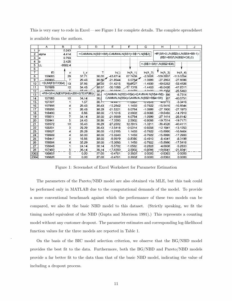
This is very easy to code in Excel— see Figure 1 for complete details. The complete spreadsheet

is available from the authors.

Figure 1: Screenshot of Excel Worksheet for Parameter Estimation

The parameters of the Pareto/NBD model are also obtained via MLE, but this task could

be performed only in MATLAB due to the computational demands of the model. To provide

a more conventional benchmark against which the performance of these two models can be

compared, we also fit the basic NBD model to this dataset. (Strictly speaking, we fit the

timing model equivalent of the NBD (Gupta and Morrison 1991).) This represents a counting

model without any customer dropout. The parameter estimates and corresponding log-likelihood

function values for the three models are reported in Table 1.

On the basis of the BIC model selection criterion, we observe that the BG/NBD model

provides the best fit to the data. Furthermore, both the BG/NBD and Pareto/NBD models

provide a far better fit to the data than that of the basic NBD model, indicating the value of

including a dropout process.

11

BG/NBD NBD Pareto/NBDr 0.243 0.385 0.553α 4.414 12.072 10.578a 0.793b 2.426s 0.606β 11.669LL −9582.4 −9763.7 −9595.0BIC 19195.9 19542.9 19221.1

Table 1: Model Estimation Results

In Figure 2, we examine the fit of these models visually: the expected numbers of people

making 0, 1, . . . , 7+ repeat purchases in the 39-week model calibration period from three models

are compared to the actual frequency distribution. The fits of the three models are very close.

On the basis of the chi-square goodness-of-fit test, we note that the BG/NBD model provides

the best fit to the data (χ23 = 4.82, p = 0.19); for the Pareto/NBD, χ2

3 = 11.99, (p = 0.007); and

the NBD fits the histogram surprisingly well, χ25 = 10.27, (p = 0.07).

0 1 2 3 4 5 6 7+0

500

1000

1500

# Transactions

Fre

quen

cy

ActualBG/NBDPareto/NBDNBD

Figure 2: Predicted versus Actual Frequency of Repeat Transactions

The relative performance of these models becomes more apparent when we consider how well

the models track the actual number of repeat transactions over time. In Figure 3 we consider the

cumulative number of repeat transactions. We immediately observe that the NBD not only fails

to track actual sales in the 39-week calibration period, but also deviates significantly from the

actual sales trajectory over the subsequent 39 weeks. By the end of June 1998, the NBD model is

over-forecasting by 24%. During the 39-week calibration period, the tracking performance of the

12

BG/NBD and Pareto/NBD models is practically identical. In the subsequent 39-week forecast

period, both models track the actual sales trajectory, with the Pareto/NBD performing slightly

better than the BG/NBD (under-forecasting by 2% versus 4%), but both models demonstrate

superb tracking/forecasting capabilities.

0 10 20 30 40 50 60 70 800

1000

2000

3000

4000

5000

6000

Week

Cum

. Rpt

Tra

nsac

tions

ActualBG/NBDPareto/NBDNBD

Figure 3: Predicted versus Actual Cumulative Repeat Transactions

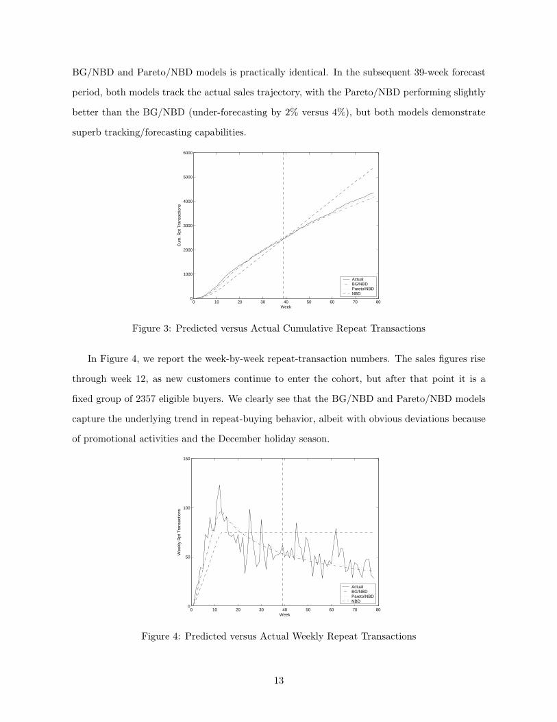
In Figure 4, we report the week-by-week repeat-transaction numbers. The sales figures rise

through week 12, as new customers continue to enter the cohort, but after that point it is a

fixed group of 2357 eligible buyers. We clearly see that the BG/NBD and Pareto/NBD models

capture the underlying trend in repeat-buying behavior, albeit with obvious deviations because

of promotional activities and the December holiday season.

0 10 20 30 40 50 60 70 800

50

100

150

Week

Wee

kly

Rpt

Tra

nsac

tions

ActualBG/NBDPareto/NBDNBD

Figure 4: Predicted versus Actual Weekly Repeat Transactions

13

Our final—and perhaps most critical—examination of the relative performance of the three

models focuses on the quality of the predictions of individual-level transactions in the forecast

period (Weeks 40–78) conditional on the number of observed transactions in the model calibra-

tion period. For the BG/NBD model, these are computed using (12). For the Pareto/NBD, as

noted earlier, the equivalent expression is represented by equation (22) in SMC. For the NBD

model, conditional expectations can be computed using the following expression (Morrison and

Schmittlein 1988):

E(Y (t) |X = x, T ) =(r + x)tα + T

where t = 39 for our analysis.

In Figure 5, we report these conditional expectations along with the average of the actual

number of transactions that took place in the forecast period, broken down by the number

of calibration-period repeat transactions. (For each x, we are averaging over customers with

different values of tx.)

0 1 2 3 4 5 6 7+0

1

2

3

4

5

6

7

8

9

10

# Transactions in Weeks 1−39

Exp

ecte

d #

Tra

nsac

tions

in W

eeks

40−

78

ActualBG/NBDPareto/NBDNBD

Figure 5: Conditional Expectations

Both the BG/NBD and Pareto/NBD models provide excellent predictions of the expected

number of transactions in the holdout period. It appears that the Pareto/NBD offers slightly

better predictions than the BG/NBD, but it is important to keep in mind that the groups towards

the right of the figure (i.e., buyers with larger values of x in the calibration period) are extremely

small. An important aspect that is hard to discern from the figure is the relative performance

14

for the very large “zero class” (i.e., the 1411 people who made no repeat purchases in the first

39 weeks). This group makes a total of 334 transactions in weeks 40–78, which comprises 18%

of all of the forecast period transactions. (This is second only to the 7+ group, which accounts

for 22% of the forecast period transactions.) The BG/NBD conditional expectation for the zero

class is 0.23, which is much closer to the actual average (334/1411=0.24) than that predicted

by the Pareto/NBD (0.14).

Nevertheless, these differences are not necessarily meaningful. Taken as a whole across

the full set of 2357 customers, the predictions for the BG/NBD and Pareto/NBD models are

indistinguishable from each other and from the actual transaction numbers. This is confirmed

by a three-group ANOVA (F2,7068 = 2.65), which is not significant at the usual 5% level. (As is

made obvious in Figure 5, the conditional expectations for the NBD differ quite significantly from

the two dropout models and the actual data.) This is an important test that demonstrates the

high degree of validity of both models, particularly for the purposes of forecasting a customer’s

future purchasing, conditional on his past buying behavior.

7 Discussion

Many researchers have praised the Pareto/NBD model for its sensible behavioral story, its

excellent empirical performance, and the useful managerial diagnostics that arise quite naturally

from its formulation. We fully agree with these positive assessments and have no misgivings

about the model whatsoever, besides its computational complexity. It is simply our intention

to make this type of modeling framework more broadly accessible so that many researchers and

practitioners can benefit from the original ideas of SMC.

The BG/NBD model arises by making a small, relatively inconsequential, change to the

Pareto/NBD assumptions. The transition from an exponential distribution to a geometric pro-

cess (to capture customer dropout) does not require any different psychological theories nor

does it have any noteworthy managerial implications. When we evaluate the two models on

their primary outcomes (i.e., their ability to fit and predict repeat transaction behavior), they

are effectively indistinguishable from each other.

15

As Albers (2000) notes, the use of marketing models in actual practice is becoming less

of an exception, and more of a rule, because of spreadsheet software. It is our hope that the

ease with which the BG/NBD model can be implemented in a familiar modeling environment

will encourage more firms to take better advantage of the information already contained in

their customer transaction databases. Furthermore, as key personnel become comfortable with

this type of model, we can expect to see growing demand for more complete (and complex)

models—and more willingness to commit resources to them (Urban and Karash 1971).

Beyond the purely technical aspects involved in deriving the BG/NBD model and comparing

it to the Pareto/NBD, we have attempted to highlight some important managerial aspects

associated with this kind of modeling exercise. For instance, to the best of our knowledge, this is

only the second empirical validation of the Pareto/NBD model— the first being Schmittlein and

Peterson (1994). (Other researchers (e.g., Reinartz and Kumar 2000, 2003; Wu and Chen 2000)

have employed the model extensively, but did not report any statistics about its performance in a

holdout period.) We find that the Pareto/NBD model yields extraordinarily accurate forecasts of

future purchasing, both at the aggregate level as well as at the level of the individual (conditional

on past purchasing).

Besides using these empirical tests as a basis to compare models, we also want to call more

attention to these analyses—with particular emphasis on conditional expectations—as the

proper yardsticks that all researchers should use when judging the absolute performance of

other forecasting models for CLV-related applications. It is important for a model to be able to

accurately project the future purchasing behavior of a broad range of past customers, and its

performance for the zero class is especially critical, given the typical size of that “silent” group.

Finally, the BG/NBD easily lends itself to relevant generalizations, such as the inclusion

of demographics or measures of marketing activity (Gupta 1991), but even then it would still

serve as an appropriate (and hard-to-beat) benchmark model in its basic form. For all of the

reasons discussed in this paper (e.g., parsimony, computational simplicity, and robust empirical

performance), the BG/NBD provides researchers with an excellent framework to begin their

CLV model-building efforts; we feel that it should be viewed as the right starting point for any

customer-base analysis exercise.

16

Appendix

In this appendix, we derive the expressions for E[(X(t)] and E(Y (t) |X = x, tx, T ). Central to

these derivations is Euler’s integral for the Gaussian hypergeometric function:

2F1(a, b; c; z) =1

B(b, c − b)

∫ 1

0tb−1(1 − t)c−b−1(1 − zt)−adt , c > b .

Derivation of E[X(t)]

To arrive at an expression for E[X(t)] for a randomly-chosen customer, we need to take the

expectation of (7) over the distribution of λ and p. First we take the expectation with respect

to λ, giving us

E(X(t) | r, α, p) =1p

− αr

p(α + pt)r

The next step is to take the expectation of this over the distribution of p. We first evaluate

∫ 1

0

1p

pa−1(1 − p)b−1

B(a, b)dp =

a + b − 1a − 1

Next, we evaluate

∫ 1

0

αr

p(α + pt)rpa−1(1 − p)b−1

B(a, b)dp = αr 1

B(a, b)

∫ 1

0pa−2(1 − p)b−1(α + pt)−rdp

letting q = 1 − p (which implies dp = −dq)

=(

α

α + t

)r 1B(a, b)

∫ 1

0qb−1(1 − q)a−2(1 − t

α+tq)−r

dq

which, recalling Euler’s integral for the Gaussian hypergeometric function,

=(

α

α + t

)r B(a − 1, b)B(a, b) 2F1

(r, b; a + b − 1; t

α+t

)

17

It follows that

E(X(t) | r, α, a, b) =a + b − 1

a − 1

[1 −

(α

α + t

)r

2F1(r, b; a + b − 1; t

α+t

)]

Derivation of E(Y (t) | X = x, tx, T )

Let the random variable Y (t) denote the number of purchases made in the period (T, T + t].

We are interested in computing the conditional expectation E(Y (t) |X = x, tx, T ), the expected

number of purchases in the period (T, T + t] for a customer with purchase history X = x, tx, T .

If the customer is active at T , it follows from (7) that

E(Y (t) |λ, p) =1p

− 1pe−λpt (A1)

What is the probability that a customer is active at T? Given our assumption that all

customers are active at the beginning of the initial observation period, a customer cannot drop

out before he has made any transactions; therefore,

P (active at T |X = 0, T, λ, p) = 1

For the case where purchases were made in the period (0, T ], the probability that a customer

with purchase history (X = x, tx, T ) is still active at T , conditional on λ and p, is simply the

probability that he did not drop out at tx and made no purchase in (tx, T ], divided by the

probability of making no purchases in this same period. Recalling that this second probability is

simply the probability that the customer became inactive at tx, plus the probability he remained

active but made no purchases in this interval, we have

P (active at T |X = x, tx, T, λ, p) =(1 − p)e−λ(T−tx)

p + (1 − p)e−λ(T−tx)

Multiplying this by [(1 − p)x−1λxe−λtx ]/[(1 − p)x−1λxe−λtx ] gives us

P (active at T |X = x, tx, T, λ, p) =(1 − p)xλxe−λT

L(λ, p |X = x, tx, T )(A2)

18

where the expression for L(λ, p |X = x, tx, T ) is given in (5). (Note that when x = 0, the

expression given in (A2) equals 1.)

Multiplying (A1) and (A2) yields

E(Y (t) |X = x, tx, T, λ, p) =(1 − p)xλxe−λT

(1p − 1

pe−λpt)

L(λ, p |X = x, tx, T )

=p−1(1 − p)xλxe−λT − p−1(1 − p)xλxe−λ(T+pt)

L(λ, p |X = x, tx, T )(A3)

(Note that this reduces to (A1) when x = 0, which follows from the result that a customer who

made zero purchases in the time period (0, T ] must be assumed to be active at time T .)

As the transaction rate λ and dropout probability p are unobserved, we compute E(Y (t) |X =

x, tx, T ) for a randomly chosen customer by taking the expectation of (A3) over the distribution

of λ and p, updated to take account of the information X = x, tx, T :

E(Y (t) |X = x, tx, T, r, α, a, b) =∫ 1

0

∫ ∞

0E(Y (t) |X = x, tx, T, λ, p)f(λ, p | r, α, a, b,X = x, tx, T )dλ dp (A4)

By Bayes theorem, the joint posterior distribution of λ and p is given by

f(λ, p | r, α, a, b,X = x, tx, T ) =L(λ, p |X = x, tx, T )f(λ | r, α)f(p | a, b)

L(r, α, a, b |X = x, tx, T )(A5)

Substituting (A3) and (A5) in (A4), we get

E(Y (t) |X = x, tx, T, r, α, a, b) =A − B

L(r, α, a, b |X = x, tx, T )(A6)

where

A =∫ 1

0

∫ ∞

0p−1(1 − p)xλxe−λT f(λ | r, α)f(p | a, b)dλ dp

=B(a − 1, b + x)

B(a, b)Γ(r + x)αr

Γ(r)(α + T )r+x(A7)

19

and

B =∫ 1

0

∫ ∞

0p−1(1 − p)xλxe−λ(T+pt)f(λ | r, α)f(p | a, b)dλ dp

=∫ 1

0

pa−2(1 − p)b+x−1

B(a, b)

{∫ ∞

0

αrλr+x−1e−λ(α+T+pt)

Γ(r)dλ

}dp

=Γ(r + x)αr

Γ(r)B(a, b)

∫ 1

0pa−2(1 − p)b+x−1(α + T + pt)−(r+x)dp

letting q = 1 − p (which implies dp = −dq)

=Γ(r + x)αr

Γ(r)B(a, b)(α + T + t)r+x

∫ 1

0qb+x−1(1 − q)a−2(1 − t

α+T+tq)−(r+x)

dq

which, recalling Euler’s integral for the Gaussian hypergeometric function,

=B(a − 1, b + x)

B(a, b)Γ(r + x)αr

Γ(r)(α + T + t)r+x 2F1(r + x, b + x; a + b + x − 1; t

α+T+t

)(A8)

Substituting (8), (A7) and (A8) in (A6) and simplifying, we get

E(Y (t) |X = x, tx, T, r, α, a, b) =

a + b + x − 1a − 1

[1 −

(α + T

α + T + t

)r+x

2F1(r + x, b + x; a + b + x − 1; t

α+T+t

)]

1 + δx>0a

b + x − 1

(α + T

α + tx

)r+x

20

References

Albers, Sonke (2000), “Impact of Types of Functional Relationships, Decisions, and Solutionson the Applicability of Marketing Models,” International Journal of Research in Marketing,17 (2–3), 169–175.

Balasubramanian, S., S. Gupta, W. Kamakura, and M. Wedel (1998), “Modeling Large Datasetsin Marketing,” Statistica Neerlandica, 52 (3), 303–323.

Fader, Peter S. and Bruce G. S. Hardie, (2001), “Forecasting Repeat Sales at CDNOW: A CaseStudy,” Interfaces, 31 (May–June), Part 2 of 2, S94–S107.

Gupta, Sunil (1991), “Stochastic Models of Interpurchase Time with Time-Dependent Covari-ates,” Journal of Marketing Research, 28 (February), 1–15.

Gupta, Sunil and Donald G. Morrison (1991), “Estimating Heterogeneity in Consumers’ Pur-chase Rates,” Marketing Science, 10 (Summer), 264–269.

Jain, Dipak and Siddhartha S. Singh (2002), “Customer Lifetime Value Research in Marketing:A Review and Future Directions,” Journal of Interactive Marketing, 16 (Spring), 34–46.

Lozier D.W. and F.W. J. Olver (1995), “Numerical Evaluation of Special Functions,” in WalterGautschi (ed.), Mathematics of Computation 1943–1993: A Half-Century of ComputationalMathematics, Proceedings of Symposia in Applied Mathematics, Providence, RI: AmericanMathematical Society.

Morrison, Donald G. and David C. Schmittlein (1988), “Generalizing the NBD Model for Cus-tomer Purchases: What Are the Implications and Is It Worth the Effort?” Journal ofBusiness and Economic Statistics, 6 (April), 145–159.

Mulhern, Francis J. (1999), “Customer Profitability Analysis: Measurement, Concentration,and Research Directions,” Journal of Interactive Marketing, 13 (Winter), 25–40.

Niraj, Rakesh, Mahendra Gupta, and Chakravarthi Narasimhan (2001), “Customer Profitabilityin a Supply Chain,” Journal of Marketing, 65 (July), 1–16.

Reinartz, Werner and V. Kumar (2000), “On the Profitability of Long-Life Customers in a Non-contractual Setting: An Empirical Investigation and Implications for Marketing,” Journal ofMarketing, 64 (October), 17–35.

Reinartz, Werner and V. Kumar (2003), “The Impact of Customer Relationship Characteristicson Profitable Lifetime Duration,” Journal of Marketing 67 (January), 77–99.

Schmittlein, David C., Donald G. Morrison, and Richard Colombo (1987), “Counting YourCustomers: Who They Are and What Will They Do Next?” Management Science, 33(January), 1–24.

Schmittlein, David C. and Robert A. Peterson (1994), “Customer Base Analysis: An IndustrialPurchase Process Application,” Marketing Science, 13 (Winter), 41–67.

Urban, Glen L. and Richard Karash (1971), “Evolutionary Model Building,” Journal of Mar-keting Research, 8 (February), 62–66.

Wu, Couchen and Hsiu-Li Chen (2000), “Counting Your Customers: Compounding Customer’sIn-store Decisions, Interpurchase Time, and Repurchasing Behavior,” European Journal ofOperational Research, 127 (1) 109–119.

21