Nonlinear Analysis 42 (2000) 1055–1062www.elsevier.nl/locate/na

Counting periodic solutions of the forcedpendulum equation

Rafael Ortega∗;1

Departamento de Matem�atica Aplicada, Facultad de Ciencias, Universidad de Granada,18071 Granada, Spain

Received 1 August 1998; accepted 22 September 1998

Keywords: Pendulum; Zeros; Holomorphic functions

1. Introduction

Let h be a holomorphic function with h(0) = 1. The number of zeros of h on adisk centered at the origin can be controlled by the maximum value of |h| on a largerdisk. This is a classical result in complex analysis that is sometimes called Jensen’sinequality (see for instance [4]). In [2] Il’yashenko and Yakovenko applied this resulttogether with the theory of conformal mappings to count the zeros of the solutionsof linear di�erential equations. The same techniques will be applied in this paper tothe forced pendulum equation. The result will be an upper estimate on the number ofperiodic solutions.The forced pendulum equation can be written in the form

�x + a sin x = f(t) + s; (1)

where a¿ 0, f : R→ R is a locally integrable function satisfying

f(t + 1) = f(t); a:e: t ∈R;∫ 1

0f(t) dt = 0;

and s∈R is a parameter. The periodic problem for this equation has been studied bymany authors and a very extensive list of references can be found in the survey paper

∗ Fax: +34-958-248596.E-mail address: rortega@goliat.ugr.es (R. Ortega)1 Supported by DGES PB95-1203, Spain.

0362-546X/00/$ - see front matter ? 2000 Elsevier Science Ltd. All rights reserved.PII: S0362 -546X(99)00169 -8

1056 R. Ortega / Nonlinear Analysis 42 (2000) 1055–1062

by Mawhin [5]. We recall some known facts: given a �xed function f, there exist twonumbers s− and s+, −a ≤ s− ≤ 0 ≤ s+ ≤ a, such that (1) has periodic solutions ifand only if

s− ≤ s ≤ s+:

The numbers s± depend continuously on f and it is not known if they can vanish.There are some explicit estimates on s±, valid for certain classes of forcings f.Since the equation is 2�-periodic in x, solutions that only di�er by a multiple of 2�

will be identi�ed. After this identi�cation, N [f; s] will denote the number of 1-periodicsolutions. In [8], Tarantello computed the exact value of N [f; s] when f satis�es asmallness condition and a¡ 4�2. The next result will give an upper estimate on N [f; s].In contrast to the result in [8], it will not be necessary to impose any condition on f,but the assumption on a will be more restrictive.

Theorem. Assume

a¡ 18√3: (2)

Then there exist two positive numbers �, � (depending only on a) such that for eachs∈ [s−; s+]

N [f; s] ≤ �− � ln �(s);

where �(s) = max{s+ − s; s− s−}.

The proof will provide concrete values for � and �. For instance, if a = 1, anadmissible choice is

N [f; s] ≤ 8:552− 2:558 ln �(s):The identity N [f; s]=∞ can only happen if �(s)=0 or, equivalently, if s=s+=s−=0.If such a situation can ever occur, the set of solutions should be a one-dimensionalcontinuum. This was proved by Serra et al. [7]. It is possible to �nd functions f suchthat N [f; 0] can be made arbitrarily large (see [6]). For these functions, the number�(0) has to be very small and so the interval [s−; s+] will become arbitrarily small.To prove the theorem we shall proceed in two steps. First we present a variant of

Jensen’s inequality that is valid for periodic holomorphic functions. It follows along thelines of Lemma 1 in [2]. After this, the periodic problem for (1) will be reduced to thestudy of the real zeros of one of these periodic holomorphic functions. This reductionis achieved using the Alternative Method in a space of complex-valued functions. Therestriction imposed on a by (2) is employed to guarantee that the auxiliary equationin the Lyapunov-Schmidt reduction is uniquely solvable.

2. Zeros of periodic holomorphic functions

Given �¿ 0 let B� be the horizontal strip of the complex plane de�ned as

B� = {z ∈C | |Imz|¡�}:

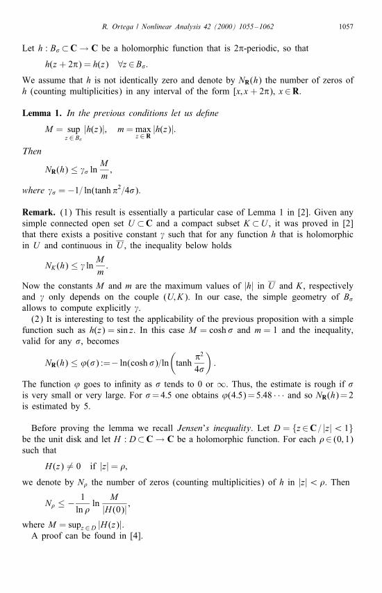
R. Ortega / Nonlinear Analysis 42 (2000) 1055–1062 1057

Let h : B� ⊂C→ C be a holomorphic function that is 2�-periodic, so thath(z + 2�) = h(z) ∀z ∈B�:

We assume that h is not identically zero and denote by NR(h) the number of zeros ofh (counting multiplicities) in any interval of the form [x; x + 2�), x∈R.

Lemma 1. In the previous conditions let us de�ne

M = supz∈ B�

|h(z)|; m=maxz∈R

|h(z)|:

Then

NR(h) ≤ � lnMm

;

where � =−1= ln(tanh �2=4�).

Remark. (1) This result is essentially a particular case of Lemma 1 in [2]. Given anysimple connected open set U ⊂C and a compact subset K ⊂U , it was proved in [2]that there exists a positive constant such that for any function h that is holomorphicin U and continuous in U , the inequality below holds

NK (h) ≤ lnMm

:

Now the constants M and m are the maximum values of |h| in U and K , respectivelyand only depends on the couple (U;K). In our case, the simple geometry of B�

allows to compute explicitly .(2) It is interesting to test the applicability of the previous proposition with a simple

function such as h(z) = sin z. In this case M = cosh � and m = 1 and the inequality,valid for any �, becomes

NR(h) ≤ ’(�) :=− ln(cosh �)=ln(tanh

�24�

):

The function ’ goes to in�nity as � tends to 0 or ∞. Thus, the estimate is rough if �is very small or very large. For �=4:5 one obtains ’(4:5)=5:48 · · · and so NR(h)=2is estimated by 5.

Before proving the lemma we recall Jensen’s inequality. Let D = {z ∈C = |z|¡ 1}be the unit disk and let H : D⊂C→ C be a holomorphic function. For each �∈ (0; 1)such that

H (z) 6= 0 if |z|= �;

we denote by N� the number of zeros (counting multiplicities) of h in |z|¡�. Then

N� ≤ − 1ln �

lnM

|H (0)| ;

where M = supz∈D |H (z)|.A proof can be found in [4].

1058 R. Ortega / Nonlinear Analysis 42 (2000) 1055–1062

Proof. It is not restrictive to assume

|h(0)|=maxz∈R

|h(z)|:This is achieved with a translation z → z − z0.The strip B� can be transformed conformally in the disk D in a standard way (see

for example [3]). The mapping

1 : z → w; w = exp(�z=2�)transforms B� onto H = {w∈C |R w¿ 0}. After this, the mapping

2 : w → �; �=w − 1w + 1

transforms H onto D. Moreover, the set K = [− �; �] becomesK1 = 1(K) = [exp(−�2=2�); exp(�2=2�)]

and

K2 = 2(K1) = [− tanh(�2=4�); tanh(�2=4�)]:The conclusion of the lemma follows after applying Jensen’s inequality to the function

H : D → C; H (�) = h(z); �= 2 ◦ 1(z):

Since H is not constant, � can be chosen as any arbitrary number satisfying

1¿�¿ tanh(�2=4�); H (�) 6= 0 if |�|= �:

3. The complex pendulum equation

In this section we consider Eq. (1) in the complex plane. This is understood in thefollowing sense: the independent variable t remains real but the unknown can takecomplex values. To emphasize this point of view we change the notation and rewrite(1) in the form

�z + a sin z = f(t) + s: (3)

This is equivalent to the real system

�x + a sin x cosh y = f(t) + s; �y + a cosh x sinh y = 0:

Our �rst task will be to formulate the periodic problem for (3) in an abstract setting.Let X be the complex Banach space of continuous and periodic functions

z : R→ C; t → z(t); z(t + 1) = z(t) ∀t ∈Rwith norm

‖z‖=maxt ∈R

|z(t)|:Given z ∈X , the mean value is denoted as

�z =∫ 1

0z(t) dt

R. Ortega / Nonlinear Analysis 42 (2000) 1055–1062 1059

and X0 is the hyperplane de�ned by the equation

�z = 0:

The space X is splitted as X = C ⊕ X0 and each z ∈X is decomposed as z = � + wwith �=�z ∈C and w∈X0.Finally, we de�ne the operators

L : X → X0; p → w;

where w(t) is the unique periodic solution of

�w = p(t)−�p; �w = 0;

and

N : X → X; Nz(t) = sin z(t):

The search of 1-periodic solutions of (3) is equivalent to the system

a∫ 1

0sin(�+ w(t)) dt = s; (4)

w =−aLN (�+ w) + F; (5)

where the unknown is (�; w)∈C × X0 and F is the unique function in X0 satisfying�F(t) = f(t), a.e. t ∈R.We shall solve the auxiliary equation (5) for �xed �. To do this we need the value

of the norm of L.

Lemma 2. ‖L‖= 1=18√3.

Proof. Given p∈X and w∈X0 with �w(t) = p(t)−�p, we wish to estimate ‖w‖ interms of ‖p‖. After a translation, we can assume |w(0)|= ‖w‖.Consider the function

�(t) = 12 t(1− t)− 1

12 ; t ∈ [0; 1]:It satis�es

�(0) = �(1); �̇(0) =−�̇(1) = 12 ;

��=−1;∫ 1

0�= 0:

An integration by parts leads to the identities∫ 1

0p�=

∫ 1

0(p−�p)�=

∫ 1

0�w�= w(0) +

∫ 1

0w ��= w(0):

Thus,

‖w‖= |w(0)| ≤(∫ 1

0|�|)‖p‖= 1

18√3‖p‖;

1060 R. Ortega / Nonlinear Analysis 42 (2000) 1055–1062

and this implies ‖L‖ ≤ 1=18√3. To prove the reversed inequality it is su�cient to

consider a sequence pn ∈X with

‖pn‖= 1; pn(t)→ sign(�(t)); a:e: t ∈ (0; 1):A passage to the limit in the identity∫ 1

0pn�= wn(0)

shows that ‖L‖ ≥ 1=18√3.

Remark. If L is restricted to X0 then the previous estimate can be improved. Actually,

‖Lp‖ ≤ 132‖p‖ ∀p∈X0:

This constant is optimal and was computed in [1, p. 139]. The previous proof stillworks in this case if one replaces � by

�∗(t) = 12 t(1− t)− 3

32 :

Given �¿ 0 we de�ne

� = {w∈X0 | |Imw(t)|¡� ∀t ∈R}:We shall solve (5) for �∈B� and w∈�, where � and � satisfy

a‖L‖ sinh(� + �)¡�; (6)

a‖L‖ cosh(� + �)¡ 1: (7)

These inequalities hold for certain small � and �. This is a consequence of (2), thatimplies

a‖L‖¡ 1:

The following estimates are consequences of some of the elementary properties of thesine function. Given �∈B� and w; w1; w2 ∈�,

|Im sin(�+ w(t))| ≤ sinh(� + �); t ∈R; (8)

|sin(�+ w1(t))− sin(�+ w2(t))| ≤ cosh(� + �)|w1(t)− w2(t)|; t ∈R: (9)

Given �∈B� we consider the operator

T� : X0 → X0; T�w =−aLN (�+ w) + F:

Inequalities (6) and (8) imply that

T�(�)⊂�:

Moreover, from (7) and (9) we deduce that T� is a contraction in �. In consequencethere is a unique �xed point w = w� in �.

R. Ortega / Nonlinear Analysis 42 (2000) 1055–1062 1061

The function

T : B� × � ⊂C× X0 → � ⊂X0; T (�; w) = T�w

is analytic and its partial derivative with respect to w is

@wT (�; w)�=−aL(cosh(�+ w)�) ∀�∈X0:

Again (7) implies that I − @wT (�; w) is an isomorphism of X0 and we can apply theimplicit function theorem to deduce that the function

�∈B� ⊂C→ w� ∈� ⊂X0

is holomorphic.In the region B� × �, the system (4)–(5) is equivalent to the equation

a∫ 1

0sin(�+ w�(t)) dt = s:

In particular, the real-valued 1-periodic solutions of (3) will correspond to the realzeros of the holomorphic periodic function

h(�) = a∫ 1

0sin(�+ w�(t)) dt − s; �∈B�:

Since s∈ [s−; s+]⊂ [− a; a], the function satis�es the estimate

|h(�)| ≤ a cosh(� + �) + a:=M; �∈B�:

Moreover, h(R) = [s− − s; s+ − s] and

max�∈R

|h(�)|= �(s):

Thus,

N [f; s] ≤ NR(h) ≤ �( lnM − ln �(s))

and the theorem is proved with

�= � lnM; � = �:

Remark. If a= 1 inequalities (6) and (7) hold for � = 3 and �= 1. The values of �and � given in the introduction are determined from the previous identities.

Acknowledgements

I thank Juan Campos for several useful remarks.

References

[1] M.R. Herman, Sur les courbes invariantes par les di��eomorphismes de l’anneau, vol. 2, Ast�erisque, 1986,p. 144.

1062 R. Ortega / Nonlinear Analysis 42 (2000) 1055–1062

[2] Y. Il’yashenko, S. Yakovenko, Counting real zeros of analytic functions satisfying linear ordinarydi�erential equations, J. Di�erential Equations 126 (1996) 87–105.

[3] M. Lavrentiev, B. Chavat, M�ethodes de la th�eorie des fonctions d’une variable complexe, Mir, Moscou.[4] A.I. Markushevich, Theory of Functions of a Complex Variable, vol II, Prentice-Hall, Englewood Cli�s,

NJ, 1965.[5] J. Mawhin, Seventy-�ve years of global analysis around the forced pendulum equation, in: Agarwal,

Neuman, Vosmansk�y (Eds.), Proceedings of the Conference Equadi� 9 (Brno, 1997), Masanyk Univ.,1998, pp. 115–145.

[6] R. Ortega, A forced pendulum equation with many periodic solutions, Rocky Mountain J. Math. 27(1997) 861–876.

[7] E. Serra, M. Tarallo, S. Terracini, On the structure of the solution set of forced pendulum-type equations,J. Di�erential Equations 131 (1996) 189–208.

[8] G. Tarantello, On the number of solutions for the forced pendulum equation, J. Di�erential Equations80 (1989) 79–93.