Embed Size (px)
Citation preview
Income and Beyond:
Multidimensional Poverty in six Latin American countries
Diego Battiston , Guillermo Cruces , Luis Felipe Lopez-Calva
Maria Ana Lugo , and Maria Emma Santos
Abstract
This paper studies multidimensional poverty for Argentina, Brazil, Chile, El Salvador, Mexico and
Uruguay for the period 1992–2006. The approach overcomes the limitations of the two traditional
methods of poverty analysis in Latin America (income-based and unmet basic needs) by combining
income with five other dimensions: school attendance for children, education of the household head,
sanitation, water and shelter. The results allow a fuller understanding of the evolution of poverty in
the selected countries. Over the study period, El Salvador, Brazil, Mexico and Chile experienced
significant reductions in multidimensional poverty. In contrast, in urban Uruguay there was a small
reduction in multidimensional poverty, while in urban Argentina the estimates did not change
significantly. El Salvador, Brazil and Mexico, and rural areas of Chile display significantly higher
and more simultaneous deprivations than urban areas of Argentina, Chile and Uruguay. In all
countries, access to proper sanitation and education of the household head are the highest
contributors to overall multidimensional poverty.
Keywords: Multidimensional poverty measurement, counting approach, Latin America, Unsatisfied
Basic Needs, rural and urban areas.
JEL Classification: D31, I32, O54.
London School of Economics and Centro de Estudios Distributivos Laborales y Sociales (CEDLAS), Universidad
Nacional de La Plata, Argentina. Centro de Estudios Distributivos Laborales y Sociales (CEDLAS)-Universidad Nacional de La Plata (UNLP) and
Consejo Nacional de Investigaciones Cientificas y Técnicas (CONICET), Argentina. World Bank
World Bank
Consejo Nacional de Investigaciones Científicas y Técnicas (CONICET)-Universidad Nacional del Sur, Argentina, and
Oxford Poverty and Human Development Initiative (OPHI), Oxford University. Corresponding autor:
1
1. Introduction
This study contributes to the longstanding literature on poverty analysis in Latin America. This
literature is mostly based on either the Unsatisfied Basic Needs (UBN) approach or on income
poverty. The former approach was promoted in the region by the United Nation’s Economic
Commission for Latin America and the Caribbean (ECLAC) and used extensively since the
beginning of the 1980s (Feres and Mancero, 2001).1 The latter was spurred by the development of
calorie consumption-based national poverty lines derived from consumption and expenditure surveys
(Altimir, 1982). These two approaches have a series of advantages and disadvantages that
differentiate them. The UBN approach aggregates a set of disparate indicators of living standard such
as construction material of the dwelling, number of people per room, access to sanitary services, and
the level of education and economic capacity of household members (generally the household head),
while the income approach has the advantage of dealing with a homogeneous indicator (although this
entails a large number of decisions and assumptions along its computation). However, both share the
same crudeness in the aggregation methodology when reporting headcount ratios.
This study provides an analysis of poverty which combines the strengths of the two traditions – the
relevance of the underlying dimensions – by means of a more sophisticated approach: income and
other indicators are combined based on sound principles of distributive analysis. This document not
only contributes to a fuller understanding of the characteristics of poverty in the region, but its results
are also relevant to creating the targeting tools that effective social programmes require.2
The existing studies on multidimensional poverty in Latin America that go beyond the Unsatisfied
Basic Need approach are few and are all country specific. Amarante et al. (2010) analyse the
evolution of poverty in Montevideo, Uruguay, between 2004 and 2006 using three alternative
methodologies: Bourguignon and Chakravarty (2003), the fuzzy sets approach (Lemmi, 2005;
Chiappero-Martinetti, 2000) and the stochastic dominance approach (Duclos, Sahn and Younger,
2006). The authors find that all methods agree that multidimensional poverty has decreased, with the
exception of stochastic dominance when income is excluded from the set of dimensions of well-
being. Also on Uruguay, Arim and Vigorito (2007) compare the evolution of income poverty among
households with children between 1991 and 2005 with that of multidimensional poverty using the
Bourguignon and Chakravarty (2003) family of indices. They find that the evolution of
multidimensional poverty over time is smoother than that of income poverty, as the first one includes
less volatile indicators. Finally, the Bourguignon and Chakravarty family of indices is also employed
in a study on Argentina for the period around the last financial crisis. Conconi and Ham (2007)
compute multidimensional poverty measurements between 1998 and 2002 using four dimensions:
dwelling, education, employment and income. The authors find that the increased deprivation in the
last two dimensions is behind the rising trend in poverty in the study period.
A number of other studies propose alternative measures of multidimensional poverty to study Latin
American countries. Paes de Barros et al. (2006) suggest using a weighted average of dichotomous
indicators of deprivations as a multidimensional poverty measure for Brazil. They apply the measure
to the national periodic household survey, including 48 indicators associated with six poverty
dimensions. The authors find a monotonic decreasing trend in multidimensional poverty between
1 The approach was also implemented by the World Bank in other developing regions of the world since 1978 (Streeten
et al., 1981). 2 Indeed, a growing number of social policy initiatives in Latin America are based on multidimensional indicators – for
instance, for the identification of beneficiaries of the Progresa/Oportunidades conditional cash transfer program in
Mexico and in the SISBEN targeting system in Colombia.
2
1993 and 2003. Calvo (2008) proposes a measure of vulnerability to multidimensional poverty and
exemplifies it using Peruvian data. Ballon and Krishnakumar (2008) develop a multidimensional
capability deprivation index based on structural equation modeling. The ‘freedom to choose’ in each
capability domain is modeled as a latent variable, partially observed by a set of indicators and
explained by a set of exogenous variables. The model is applied to a household survey dataset for
Bolivia in 2002, focusing on two capability domains of children: knowledge and living conditions.
The authors find a strong interdependence between the two studied dimensions. Lopez-Calva and
Rodriguez-Chamussy (2005) and Lopez-Calva and Ortiz-Juarez (2009) have also adopted a
multidimensional approach to studying poverty in Mexico. They estimate the magnitude of the
‘exclusion error’ in targeting programmes when a monetary measure is adopted instead of a
multidimensional one. They find a large variability in the exclusion error depending on the selected
criterion to identify the multidimensionally poor (union vs. intersection, explained in the next
section). The Mercosur Human Development Report 2009-2010 developed a multidimensional
poverty index for young people (15-29 years old) for the four Mercosur’s countries, implementing
the Alkire and Foster methodology (PNUD, 2009). Finally, since 2004, the Programa Observatorio
de la Deuda Social Argentina (Pontificia Universidad Catolica Argentina) implements a survey
which collects information on housing conditions, health and subsistence and computes a composite
indicator of deprivation constructed using principal components analysis.
The present paper analyses the evolution of multidimensional poverty in six Latin American
countries (Argentina, Brazil, Chile, El Salvador, Mexico and Uruguay). The contribution of this
study is twofold. First, we make over-time and cross-country poverty comparisons using two existing
multidimensional measures – those of Bourguignon and Chakravarty (BC) (2003) and the
Unsatisfied Basic Needs index – and a new multidimensional poverty index proposed by Alkire and
Foster (AF)(2007, 2011), built in the spirit of the capability approach. Second, we use a unique
dataset based on comparable data sources and indicators for the six countries. This allows the
comparisons of the evolution of poverty across countries. The analysis and evidence presented
contribute to the documentation of the diversity of experiences in terms of poverty reduction in the
countries and period under study – Argentina, Brazil, Chile, El Salvador, Mexico and Uruguay from
the early 1990s to the mid- 2000s.
The poverty measures used in this paper have been presented in the introduction of this special issue.
Thus, the rest of the paper is organised as follows. Section 2 presents the dataset, the selected
dimensions and indicators, as well as the thresholds and weights employed in the analysis. Section 3
discusses the empirical results, and Section 4 provides some concluding remarks.
2. Datasets, Dimensions, Poverty Lines and Weights
2.1 Dataset
The dataset used in this paper corresponds to the Socioeconomic Database for Latin America and the
Caribbean (SEDLAC), constructed by the Centro de Estudios Distributivos Laborales y Sociales
(CEDLAS) and the World Bank. The dataset comprises household surveys of different Latin
American countries which have been homogenised to make variables comparable across countries –
the details of this process are covered in CEDLAS (2009). The present research concentrates on a
subset of the available database to maximize the possibilities for comparison across time and
between countries. The study covers Argentina, Brazil, Chile and Uruguay, El Salvador and Mexico.
Altogether, they account for about 64 per cent of the total population in Latin America in 2006.

3
The paper performs estimates at five points in time between 1992 and 2006 for each country. In the
case of Argentina and Uruguay, the data are representative of urban areas only.3 In the other four
countries data are nationally representative, including information from both urban and rural areas.
In each country data corresponds to six point observations between 1991 and 2006; in most cases the
years coincide across countries. Full details of survey names, sample sizes precise estimation years
can be found in Table A.1 in the Appendix.. The definition of ‘rural areas’ by the surveys performed
in each of these four countries is fairly similar.4 In each country, only households with complete
information on all variables and consistent answers on income were considered.
2.2 Dimensions and Indicators
The selection of dimensions and indicators constitutes a crucial step in the process of defining a
multidimensional poverty measure, and there has been significant discussion on the best procedures
to follow (Alkire, 2002, 2008, Alkire and Santos, 2009 for a summary). In this paper we do not
intend to prescribe a list of indicators that should constitute a multidimensional poverty measure for
Latin America. The aim is much more modest in that respect: we intend to look at the evolution and
current state of indicators that have traditionally constituted measures of poverty in the region and
put them together in better aggregate measures. Yet, the tradition for using these indicators has well-
founded reasons.
In the mid- 1970s a new approach to development issues started to gain consensus: the basic needs
approach. The Declaration of Cocoyoc (1974) presented by two United Nations bodies (UNCTAD
and UNEP)5 was echoed by the 1976 International Labour Organisation’s World Employment
Conference Meeting Basic Needs: Strategies for Eradicating Mass Poverty and Unemployment (ILO,
1976) and the 1976 Report of the Dag Hammarskjöld Foundation, What Now: Another Development.
The approach was also supported within the Latin America region by the Bariloche Project’s
Catastrophe or New Society? (Herrera et al., 1976). All these reports, books and declarations pointed
to the need for prioritizing the satisfaction of the basic human needs in the development agenda. In
1978, the World Bank started to foster this approach, promoting a series of country studies. The
approach constituted a powerful and important idea that shifted the attention of the development
thinking away from growth and its assumed ‘trickle downs’ to removing mass deprivation.
Although it was recognised that it was not possible to reach complete agreement on the list of basic
needs, a few were consistently mentioned: ‘... some needs are common to the poor in most countries
– these include food and nutrition, health services, education, water, sanitation and shelter. These are
basic human needs in large part because they contribute to two fundamental aspects of human life –
health and education’ (Stewart 1980). In order to monitor progress, ECLAC adopted this approach
to measure poverty, which became known as the Unsatisfied Basic Needs or the ‘direct’ method to
measure poverty, as opposed to the ‘indirect method’, based on household income. The UBN method
was implemented using census data. The level of disaggregation of census data allowed the
3 Both Argentina and Uruguay are highly urbanized countries, with an urban population share of 87 and 92 per cent
correspondingly. In the case of Argentina, the survey currently covers about 61 per cent of the total population in the country. However, over the years, the survey has progressively incorporated urban areas. For comparability reasons we work with the 15 urban agglomerations that were included since 1992. These urban areas represent 45.7 per cent of the total country population. The survey in Uruguay covers about 80 per cent of the total country population. 4 In Chile it corresponds to localities of less than 1,000 people or with 1,000 to 2,000 people, of which most perform primary activities. In Mexico it refers to localities of less than 2,500 people. In Brazil, rural areas are not defined according to population size but rather they are all those not defined as urban agglomerations by the Brazilian Institute of Geography and Statistics. In El Salvador, rural areas are all those outside the limits of municipalities heads, which are populated centres where the administration of the municipality is located. Again, this definition does not refer to any particular population size. 5 UNCTAD is the United Nations Conference on Trade and Development, and UNEP is the United Nations Environment Programme.
4
construction of poverty maps.6 However, some compromises had to be made in terms of the
indicators to be considered. In particular, censuses do not typically incorporate indicators of health
such as nutrition or mortality. Thus, this had to be proxied by access to water and sanitation, which
were in the indicators of basic needs themselves. Such approximation is actually incomplete, yet at
least it captures part of the health threats. There is ample evidence on the positive impact that safe
water and improved sanitation have on reducing the prevalence of a number of diseases, some of
which are direct causes of child mortality.7
We draw from the tradition of the UBN approach and its gained consensus and use five indicators
typically included there. However, it has been long argued that both the direct and the indirect
methods capture partial aspects of poverty (Feres and Mancero, 2001; Boltvinik, 1990), that both the
income dimension as well as the UBN indicators are relevant for assessing well-being, and that there
are significant errors in targeting the poor (either of inclusion or exclusion) when only one of them is
used. 8
Thus, given the availability of the income indicator in household surveys, we incorporate it in
our measurement, as a complement of the others, constituting what can be seen as a hybrid method. 9
Table 1 presents the indicators selected to perform the poverty estimates. For income, the World
Bank’s poverty line of US$2 per capita per day was selected. It is acknowledged that this is a rather
conservative poverty line for Latin America, but it guarantees full comparability across countries.10
Children’s education is another indicator considered, requiring all children between 7 and 15 years
old (inclusive) to be attending school. This indicator belongs to the UBN approach. Households with
no children are considered non-deprived in this indicator.11
A third indicator refers to the educational
level of the household head, with the threshold set at five years of education. Again this indicator is
part of the UBN approach, although in that approach the required threshold is the second grade of
primary school and it is usually part of a composite indicator together with the dependency index of
the household (considered to be deprived if there are four or more people per employed member).
Two years of education seemed a very low threshold, so five years were used instead. Also, given
that the income indicator is being included, the high dependency index seemed less relevant in this
hybrid approach. Additionally, it is worth noting that the education of the household head is a stock
variable; it is very unlikely to change in the short run. The other three indicators used relate to the
dwelling’s conditions and are also UBN indicators: having proper sanitation (flush toilet or pit
6 For most countries in the region there are UBN estimates with the 1980, 1990 and 2000 censuses. 7 For example, water, sanitation, and hygiene interventions reduce diarrhoeal disease on average by between one-quarter and
one-third. According to the WHO, diarrhoea causes 2.2 million deaths every year mostly among children under the age of
five. Safe water is estimated to reduce the median infection rate of trachoma by 25 per cent. It has also been found that well designed water and sanitation interventions reduce by 77 per cent the median infection rate of schistosomiasis. Finally, cholera can also be prevented with access to safe drinking water (WHO, 2000). 8 Cruces and Gasparini (2008) illustrate these inclusion and exclusion effects by studying the targeting of cash transfer programs based on a combination of income and other UBN-related indicators. 9 This ‘hybrid method’ can be criticized for potential double-counting, arguing that dimensions that may have been
considered in the basic consumption basket used to determine the poverty line are included again as a separate indicator. However, in this dataset, the Spearman correlations between income and the other different indicators are relatively low (not exceeding 0.5 in any case) and decrease over time, suggesting that a multidimensional approach does indeed incorporate new elements to poverty analysis. Table A.2 in the Appendix reports these correlations. 10
This poverty line is prior to the latest amendment by the World Bank (Ravallion, Chen and Sangraula, 2009), which raised this line from approximately from US$2.15 to US$2.50. The impact of this change in the poverty line differs across countries. In Argentina, Brazil, Chile and Uruguay it produced an increase in the income poverty estimates, whereas in El Salvador and Mexico it produced a decrease in the income poverty estimates. Therefore the income deprivation rates reported in this paper should be taken as a lower bound in the first group of countries and as an upper bound in the second. This does not alter the conclusions of this paper. 11
Note that this is also the approach taken in the Multidimensional Poverty Index developed by Alkire and Santos (2010) for the 2010 Human Development Report.
5
latrine), living in a shelter with non-precarious wall materials and having access to running water in
the dwelling.
It is worth recognising that the six considered indicators are less than perfect. They are all indicators
of access to resources but provide no guarantee that the person actually enjoys good nutrition and
education for example. Sen’s capability approach – developed later than the basic needs approach –
argues the importance of considering the person’s functionings – that is – the actual abilities she has
to pursue the life she values and has reason to value (Sen, 1992, 1999). ‘To understand that the
means of satisfactory human living are not themselves the ends of good living helps to bring about a
significant extension of the reach of the evaluative exercise’ (Sen, 2009, p. 234). Moreover, Sen
argues that the list of capabilities (defined as the set of functionings) to be included in such
evaluative exercises should be developed through participatory processes and public reasoning (Sen,
2009). Unfortunately, we are limited by the data in including indicators of functionings, but we
consider that these ideas should guide future developments in the design of household surveys.
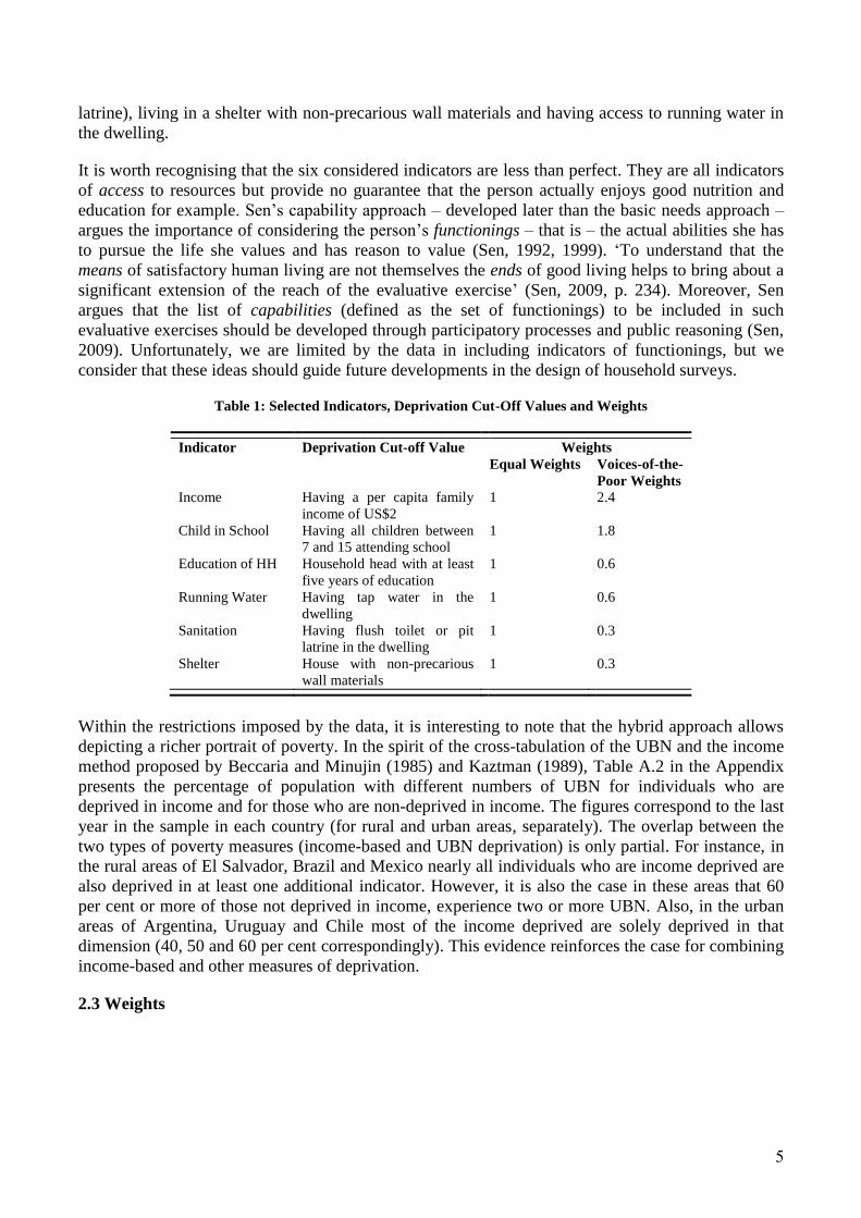
Table 1: Selected Indicators, Deprivation Cut-Off Values and Weights
Indicator Deprivation Cut-off Value Weights
Equal Weights Voices-of-the-
Poor Weights
Income Having a per capita family
income of US$2
1 2.4
Child in School Having all children between
7 and 15 attending school
1 1.8
Education of HH Household head with at least
five years of education
1 0.6
Running Water Having tap water in the
dwelling
1 0.6
Sanitation Having flush toilet or pit
latrine in the dwelling
1 0.3
Shelter House with non-precarious
wall materials
1 0.3
Within the restrictions imposed by the data, it is interesting to note that the hybrid approach allows
depicting a richer portrait of poverty. In the spirit of the cross-tabulation of the UBN and the income
method proposed by Beccaria and Minujin (1985) and Kaztman (1989), Table A.2 in the Appendix
presents the percentage of population with different numbers of UBN for individuals who are
deprived in income and for those who are non-deprived in income. The figures correspond to the last
year in the sample in each country (for rural and urban areas, separately). The overlap between the
two types of poverty measures (income-based and UBN deprivation) is only partial. For instance, in
the rural areas of El Salvador, Brazil and Mexico nearly all individuals who are income deprived are
also deprived in at least one additional indicator. However, it is also the case in these areas that 60
per cent or more of those not deprived in income, experience two or more UBN. Also, in the urban
areas of Argentina, Uruguay and Chile most of the income deprived are solely deprived in that
dimension (40, 50 and 60 per cent correspondingly). This evidence reinforces the case for combining
income-based and other measures of deprivation.
2.3 Weights
6
The weighting of indicators also constitutes a challenge when constructing a multidimensional
poverty measure since they reflect the relative value of the different considered dimensions.12
Both
statistical and normative weights have been used in the literature. Normative weights have the
advantage of being more transparent and allowing comparisons over time. When discussing the
selection and aggregation of social indicators for Europe, Atkinson et al. (2002) have argued in
favour of a balanced portfolio of indicators across different dimensions and of proportionate weights
across indicators.
In this paper two alternative weighting systems are used. The first scheme weights each indicator
equally. However, it can be argued that in the set of selected indicators, more than one indicator is
associated with the same dimension. For example, water, sanitation and shelter can be associated
with a dwelling’s characteristics and the other two indicators (children attending school and the
education of the household head) refer to the dimension of education of the household.13
Therefore,
the equal weights are implicitly weighting the dwelling conditions three times, and the education
dimension twice, compared to the income dimension.
The second weighting structure is derived from a replica of a participatory study on the voices of the
poor carried out by Mexico’s Secretaría de Desarrollo Social (Székely, 2003). In this study the poor
were asked about their valuation of different dimensions. The number and variety of dimensions
included in the questionnaire exceeds those considered here; however, its results are useful for
producing a ranking of the six indicators. This weight structure (last column in Table 1) gives the
income dimension the highest weight – a weight which is 1.3 times the weight assigned to children’s
education, four times the weight placed on the education of the household head and access to running
water, and eight times the weight assigned to access to sanitation and proper shelter. These sets of
weights will be referred to in what follows as voices of the poor weights (VP weights). This
weighting system is in line with Sen’s capability approach in that it aims at weighting indicators
according to what the poor value. However, in this particular case it has some limitations. Because
the study was restricted to Mexico, this ranking should not be interpreted as necessarily representing
the poor’s values in the six countries under study. Also, a different cardinalisation of these weights
would have emerged if we had considered some of the other dimensions included in the study.
Despite these shortcomings, we understand that the VP weights offer a valuable and interesting
alternative to quantify multidimensional poverty in the region in this study.
Three of the indicators are cardinal variables (income, proportion of children in the household not
attending school and years of education of the household head) and three are dichotomous (having
running water in the household, having proper sanitation and living in a house with non-precarious
materials). If a person falls short in one of the dichotomous indicators, her poverty gap in this
indicator will be equal to one, provided she has been identified as multidimensionally poor. This
implies that for measures such as M1, M2 and the BC measures, deprivation in dichotomous
indicators will generally have by definition a higher impact than deprivation in cardinal ones. Also,
for pairs of dichotomous indicators, the substitutability or complementarity relationship does not
apply. Therefore, using dichotomous information in measures that require cardinal data is not
completely satisfactory; their difference with respect to M0 as well as their changes over time will be
dominated by the variations in the cardinal variables. Still, we present these results to obtain a rough
sense of the depth and distribution of the deprivation in these dimensions. It is also worth noting that
when VP weights are used, the two variables that receive the highest weights (income and children in
12 On the meaning of dimension weights in multidimensional indices of well-being and deprivation and alternative approaches to setting them, see Decancq and Lugo (forthcoming). 13 Note however that the distinction is not clear. As argued above, sanitation and water can be understood as proxies for health, belonging to a different dimension.

7
school) are continuous, shifting weight from dichotomous to cardinal variables, which lessens some
of the problems mentioned above.
3. Empirical Results14
3.1 Deprivation Rates by Indicator
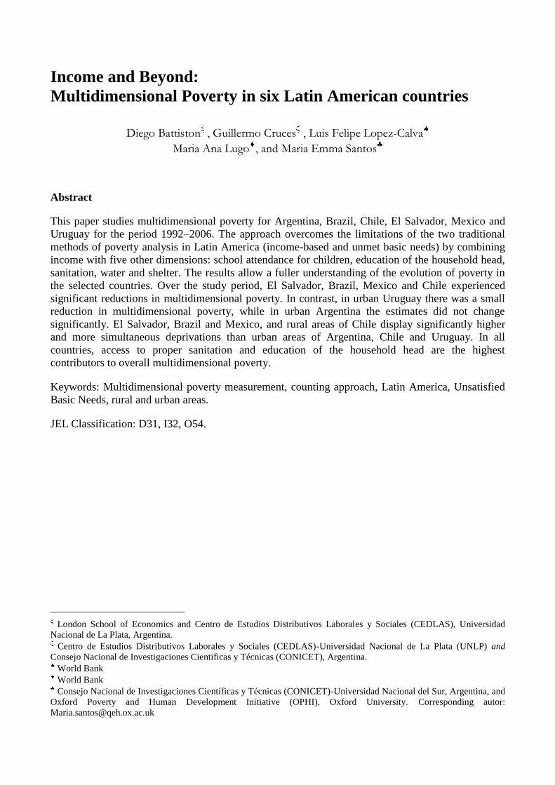
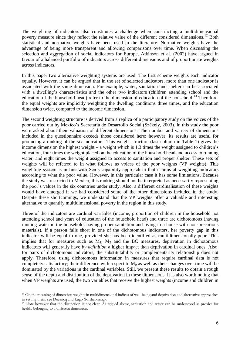
Fig. 1 presents the deprivation rates for each indicator in each country and year, in rural and urban
areas, except for Argentina and Uruguay where the rates correspond only to urban areas. Despite
being a crude poverty measure, the headcount ratio for each indicator provides a preliminary picture
of deprivation in the region. It is possible to distinguish two groups: the urban and rural areas of El
Salvador, Mexico and Brazil together with the rural areas of Chile, and the urban areas of the
southern cone countries – Argentina, Chile and Uruguay. The first group of countries and regions
exhibit much higher deprivation rates than those in the second group. In particular, El Salvador is the
country with the highest levels of deprivation in all indicators. The deprivation rates in this country
are high, not only relative to those of other countries, but also from an absolute point of view: in five
out of the six indicators, the rural areas of the country presented deprivation rates of 50 per cent or
higher in 2006. Deprivation headcounts in rural areas of El Salvador are followed by those of the
rural areas of Brazil, Mexico and Chile, and then by the urban areas of El Salvador, Brazil and
Mexico. Deprivation rates in the urban areas of Argentina, Chile and Uruguay are, for each indicator,
well below those in the aforementioned regions. It is also worth noting the disparities within
countries between urban and rural areas: deprivation rates in rural areas are at least double urban
deprivation rates. In Chile the difference is particularly marked, as if each of these areas – rural and
urban – belonged to a different country.
Comparing across indicators, three interesting features emerge. First, the indicators with the highest
headcount ratios for all countries refer to deprivations in the level of education of the household head
and sanitation. In the rural areas of El Salvador, Brazil and Mexico 70, 75 and 50 per cent of the
population, respectively, lived in a household where the household head had less than five years of
education in 2006 and 96, 80 and 68 per cent, respectively, lived in a household without access to
proper sanitation facilities. Comparable deprivation rates in respective urban areas and in rural areas
of Chile are between 22 and 45 per cent, whereas in the urban areas of Argentina, Chile and Uruguay
they do not exceed 17 per cent. Second, in all countries, income deprivation lies in the middle of the
rankings of deprivations, though rates vary significantly across countries (between 58 per cent in
rural El Salvador to 3 per cent in urban Chile). Finally, a somewhat encouraging feature is that,
although deprivation in the education level of the household head is one of the most prevalent
deprivations in all countries, the percentage of families with at least one child not attending school is
among the lowest deprivation rates.
Temporal trends are also encouraging. In almost all cases, deprivation rates declined between 1992
and 2006 and in many cases they were halved. The few exceptions are Uruguay, where income
poverty steadily increased throughout the period, and Argentina, where poverty headcounts in
income, sanitation and shelter are somewhat higher in 2006 than fifteen years before.
14 All estimates were bootstrapped using 200 replications. Detailed and complete estimates of all measures, all k cut-offs and weights, as well as their confidence intervals, are available upon request to the authors.
8
Fig. 1: Deprivation Rates by Indicator
Rural and Urban Areas, 1992–2006
0
10
20
30
40
50
60
70
80
90
10
0
% o
f D
ep
rive
d P
eo
ple
Income Child in School HH Education Sanitation Water Shelter
19921995
20002003
20061992
19952000
20032006
19921995
20002003
20061992
19952000
20032006
19921995
20002003
20061992
19952000
20032006
Argentina
01
02
03
04
05
06
07
08
09
01
00
% o
f D
epri
ve
d P
eo
ple
Income Child in School HH Education Sanitation Water Shelter
19921995
20012003
20061992
19952001
20032006
19921995
20012003
20061992
19952001
20032006
19921995
20012003
20061992
19952001
20032006
Brazil
Urban Rural
01
02
03
04
05
06
07
08
09
01
00
% o
f D
epri
ve
d P
eo
ple
Income Child in School HH Education Sanitation Water Shelter
19921996
20002003
20061992
19962000
20032006
19921996
20002003
20061992
19962000
20032006
19921996
20002003
20061992
19962000
20032006
Chile
Urban Rural
01
02
03
04
05
06
07
08
09
01
00
% o
f D
epri
ve
d P
eo
ple
Income Child in School HH Education Sanitation Water Shelter
19921996
20002004
20061992
19962000
20042006
19921996
20002004
20061992
19962000
20042006
19921996
20002004
20061992
19962000
20042006
Mexico
Urban Rural
01
02
03
04
05
06
07
08
09
01
00
% o
f D
epri
ve
d P
eo
ple
Income Child in School HH Education Sanitation Water Shelter
19911995
20002003
20051991
19952000
20032005
19911995
20002003
20051991
19952000
20032005
19911995
20002003
20051991
19952000
20032005
El Salvador
Urban Rural
01
02
03
04
05
06
07
08
09
01
00
% o
f D
ep
rive
d P
eo
ple
Income Child in School HH Education Sanitation Water Shelter
19921995
20002003
20061992
19952000
20032006
19921995
20002003
20061992
19952000
20032006
19921995
20002003
20061992
19952000
20032006
Uruguay
3.2. Multidimensional Poverty: The Multidimensional H and the M0 measure
The Multidimensional Headcount H and the Adjusted Multidimensional Headcount M0 measures
were estimated for k=1,…6, using the two weighting structures detailed above. This section focuses
on the most relevant points that can be derived from these results.
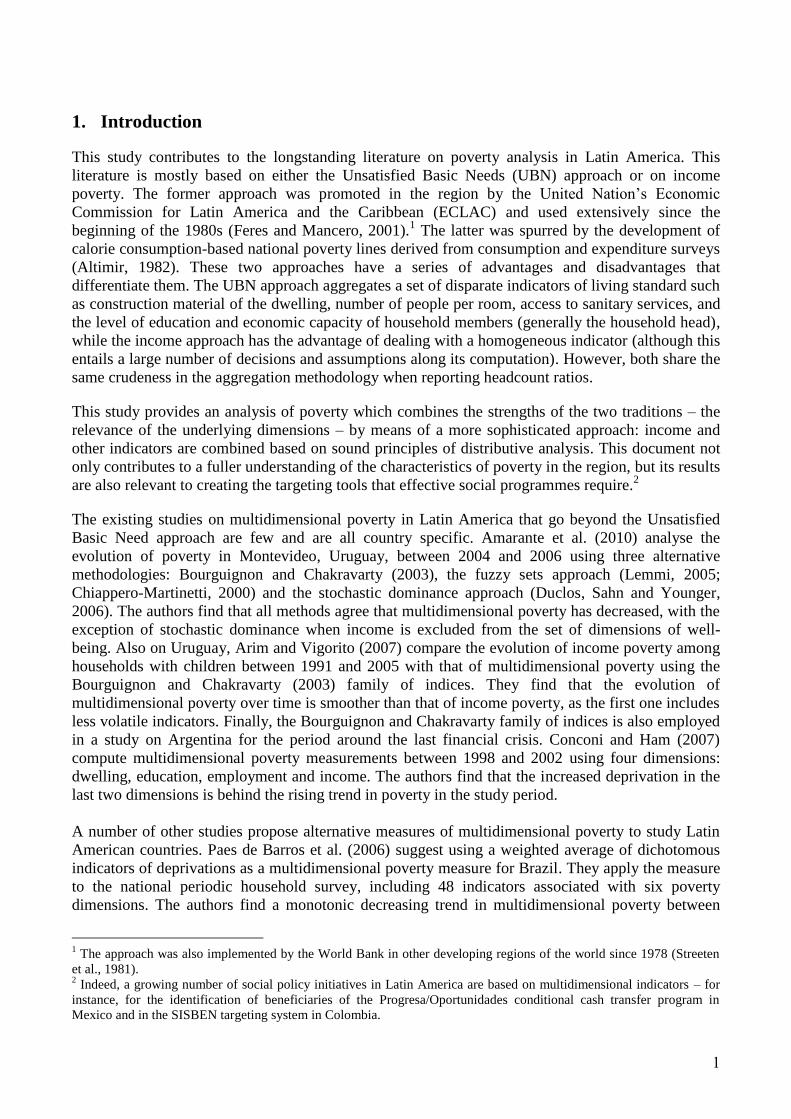
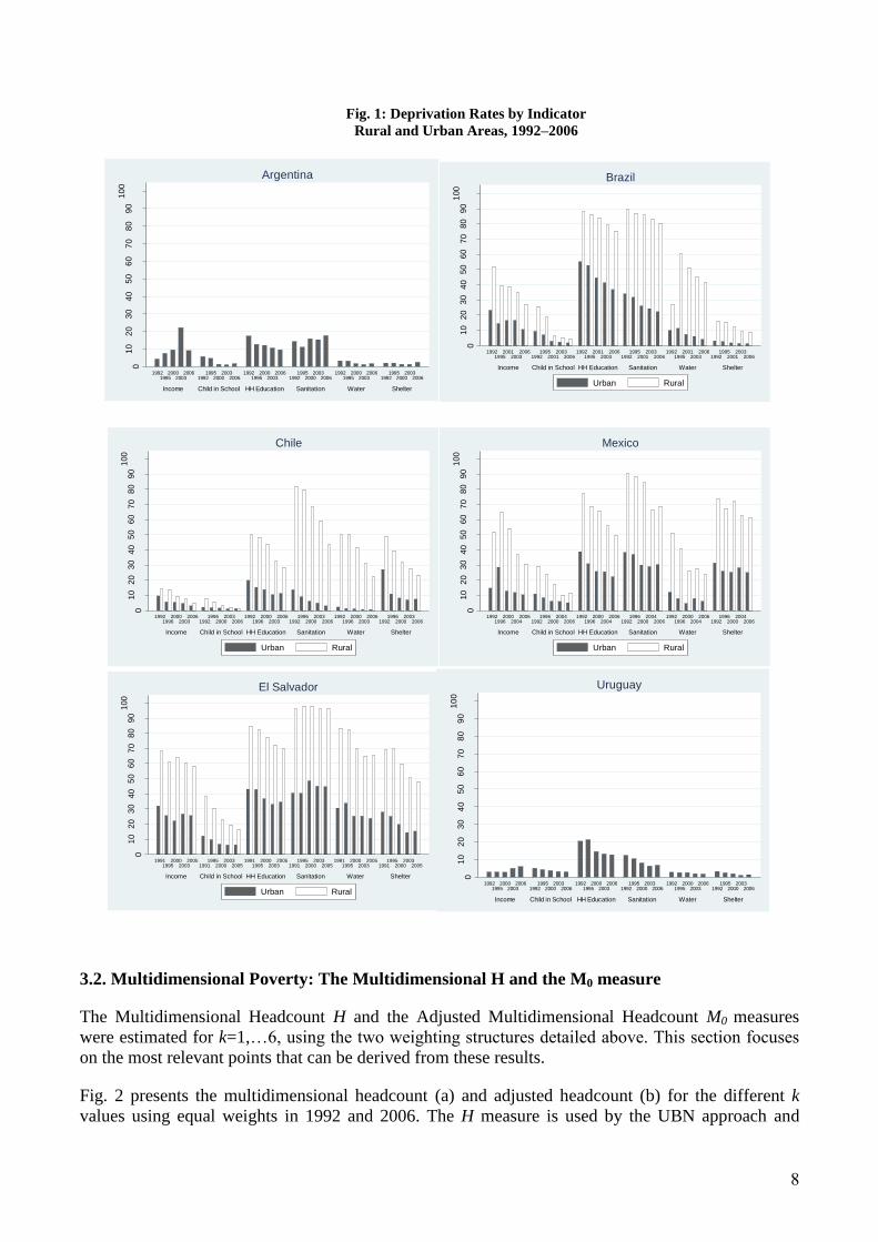
Fig. 2 presents the multidimensional headcount (a) and adjusted headcount (b) for the different k
values using equal weights in 1992 and 2006. The H measure is used by the UBN approach and
9
indicates the percentage of people deprived in one or more dimensions (k=1), two or more (k=2), and
so on. In the figure, countries are sorted according to their deprivation in 1992 when k=1.
Fig. 2: Multidimensional Poverty for Different k Values and Equal Weights
1992 and 2006
(a) Multidimensional Headcount H (b) Adjusted Multidimensional Headcount M0
010
20
30
40
50
60
70
80
90
10
0
Multid
imen
sio
na
l H
El Salvador Brazil Mexico Chile Uruguay Argentina
k=1k=2
k=3k=4
k=5k=6
k=1k=2
k=3k=4
k=5k=6
k=1k=2
k=3k=4
k=5k=6
k=1k=2
k=3k=4
k=5k=6
k=1k=2
k=3k=4
k=5k=6
k=1k=2
k=3k=4
k=5k=6
1992 2006
0
10
20
30
40
50
60
70
80
90
10
0
M0 w
ith
Eq
ua
l W
eig
hts
El Salvador Brazil Mexico Chile Uruguay Argentina
k=1k=2
k=3k=4
k=5k=6
k=1k=2
k=3k=4
k=5k=6
k=1k=2
k=3k=4
k=5k=6
k=1k=2
k=3k=4
k=5k=6
k=1k=2
k=3k=4
k=5k=6
k=1k=2
k=3k=4
k=5k=6
1992 2006
Note: Estimates in Uruguay and Argentina correspond only to urban areas.
Among the countries for which data are available for both urban and rural areas, El Salvador is the
poorest country, followed by Brazil, Mexico and then Chile. For k=1, Brazil has a higher H than
Mexico in 1992, and about the same in 2006, but for higher k values, Mexico has much higher H.
This suggests that deprivations in Mexico are more coupled than in Brazil: if one person fails to
achieve an adequate level in a given indicator, it is more likely that she will also fall short in another
indicator in Mexico than in Brazil.
Between 1992 and 2006, all countries reduced their multidimensional headcounts for all k values.
Most impressively, Chile halved its headcounts for all k values whereas El Salvador, Mexico and
Brazil achieved this sort of reduction for higher k values (k≥4). In urban Argentina, the reduction in
the multidimensional headcount was very mild and indicates that losses in some dimensions (such as
income, shelter and sanitation) are being compensated by gains in others (such as education and
water).
Using the adjusted headcount ratio M0, a measure sensitive to the breadth of poverty shown in (b) of
Fig. 2, the differences between El Salvador and the rest of the countries for which urban and rural
data are available become sharper. Not only does it exhibit the highest multidimensional poverty
levels, but it is also well above the estimates for the other countries, doubling or more the next
highest estimate for all k values. Also, once the multidimensional headcount is adjusted it becomes
more evident that Mexico is worse off than Brazil; the average number of deprivations experienced
by the poor in Mexico is higher relative to Brazil. In El Salvador, Mexico, Brazil and Chile, the
declines in M0 are larger in relative terms than those in H, most notably for lower values of k. The
interpretation of this is that not only are fewer deprived people at the end of the period but also that
those who are deprived experience fewer deprivations on average. In urban Uruguay, the reduction
of M0 was very small and virtually nil for urban Argentina. All in all, this is a promising picture in
terms of poverty for the countries considered and complements the declining trend in inequality
documented by Gasparini et al. (2008) for most countries in Latin America over the same period.
10
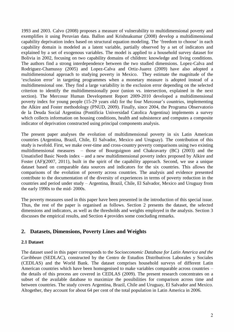
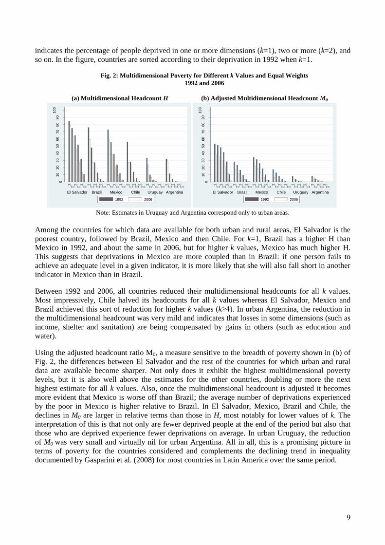
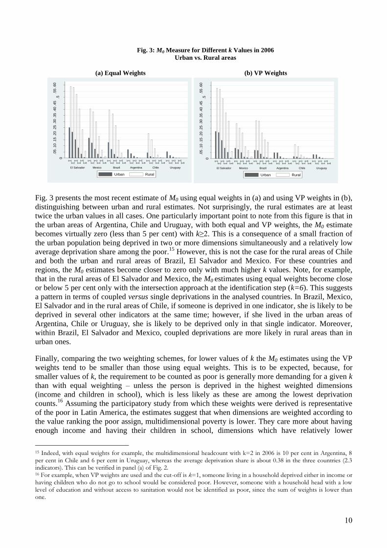
Fig. 3: M0 Measure for Different k Values in 2006
Urban vs. Rural areas
(a) Equal Weights (b) VP Weights
0
.05
.10
.15
.20
.25
.30
.35
.40
.45
.5.5
5.6
0
M0
with E
qu
al W
eig
hts
El Salvador Mexico Brazil Argentina Chile Uruguay
k=1k=2
k=3k=4
k=5k=6
k=1k=2
k=3k=4
k=5k=6
k=1k=2
k=3k=4
k=5k=6
k=1k=2
k=3k=4
k=5k=6
k=1k=2
k=3k=4
k=5k=6
k=1k=2
k=3k=4
k=5k=6
Urban Rural
0
.05
.10
.15
.20
.25
.30
.35
.40
.45
.5.5
5.6
0
M0
with V
P W
eig
hts
El Salvador Mexico Brazil Argentina Chile Uruguay
k=1k=2
k=3k=4
k=5k=6
k=1k=2
k=3k=4
k=5k=6
k=1k=2
k=3k=4
k=5k=6
k=1k=2
k=3k=4
k=5k=6
k=1k=2
k=3k=4
k=5k=6
k=1k=2
k=3k=4
k=5k=6
Urban Rural
Fig. 3 presents the most recent estimate of M0 using equal weights in (a) and using VP weights in (b),
distinguishing between urban and rural estimates. Not surprisingly, the rural estimates are at least
twice the urban values in all cases. One particularly important point to note from this figure is that in
the urban areas of Argentina, Chile and Uruguay, with both equal and VP weights, the M0 estimate
becomes virtually zero (less than 5 per cent) with k≥2. This is a consequence of a small fraction of
the urban population being deprived in two or more dimensions simultaneously and a relatively low
average deprivation share among the poor.15
However, this is not the case for the rural areas of Chile
and both the urban and rural areas of Brazil, El Salvador and Mexico. For these countries and
regions, the M0 estimates become closer to zero only with much higher k values. Note, for example,
that in the rural areas of El Salvador and Mexico, the M0 estimates using equal weights become close
or below 5 per cent only with the intersection approach at the identification step (k=6). This suggests
a pattern in terms of coupled versus single deprivations in the analysed countries. In Brazil, Mexico,
El Salvador and in the rural areas of Chile, if someone is deprived in one indicator, she is likely to be
deprived in several other indicators at the same time; however, if she lived in the urban areas of
Argentina, Chile or Uruguay, she is likely to be deprived only in that single indicator. Moreover,
within Brazil, El Salvador and Mexico, coupled deprivations are more likely in rural areas than in
urban ones.
Finally, comparing the two weighting schemes, for lower values of k the M0 estimates using the VP
weights tend to be smaller than those using equal weights. This is to be expected, because, for
smaller values of k, the requirement to be counted as poor is generally more demanding for a given k
than with equal weighting – unless the person is deprived in the highest weighted dimensions
(income and children in school), which is less likely as these are among the lowest deprivation
counts.16
Assuming the participatory study from which these weights were derived is representative
of the poor in Latin America, the estimates suggest that when dimensions are weighted according to
the value ranking the poor assign, multidimensional poverty is lower. They care more about having
enough income and having their children in school, dimensions which have relatively lower
15 Indeed, with equal weights for example, the multidimensional headcount with k=2 in 2006 is 10 per cent in Argentina, 8 per cent in Chile and 6 per cent in Uruguay, whereas the average deprivation share is about 0.38 in the three countries (2.3 indicators). This can be verified in panel (a) of Fig. 2. 16 For example, when VP weights are used and the cut-off is k=1, someone living in a household deprived either in income or having children who do not go to school would be considered poor. However, someone with a household head with a low level of education and without access to sanitation would not be identified as poor, since the sum of weights is lower than one.
11
deprivation rates, than having access to sanitation and a household head with five or more year of
education, dimensions which have relatively higher deprivation rates.
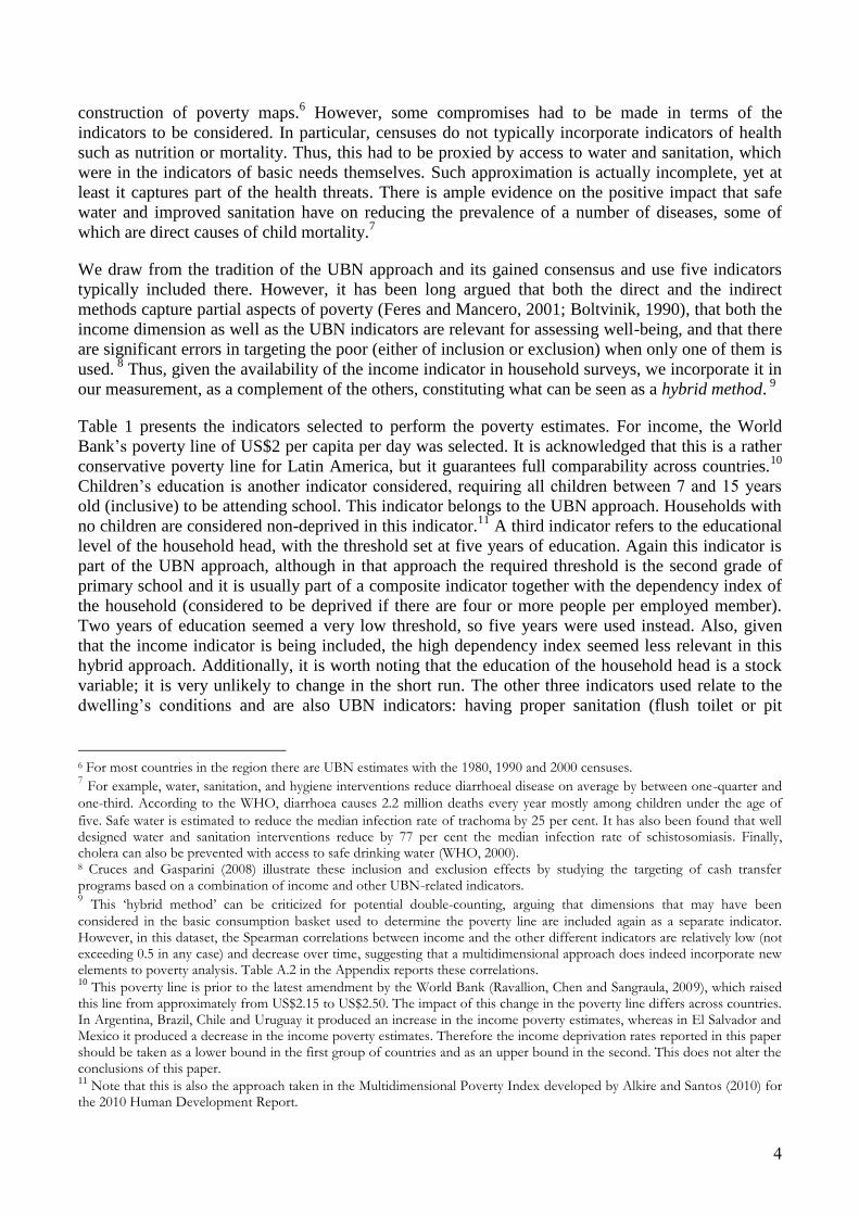
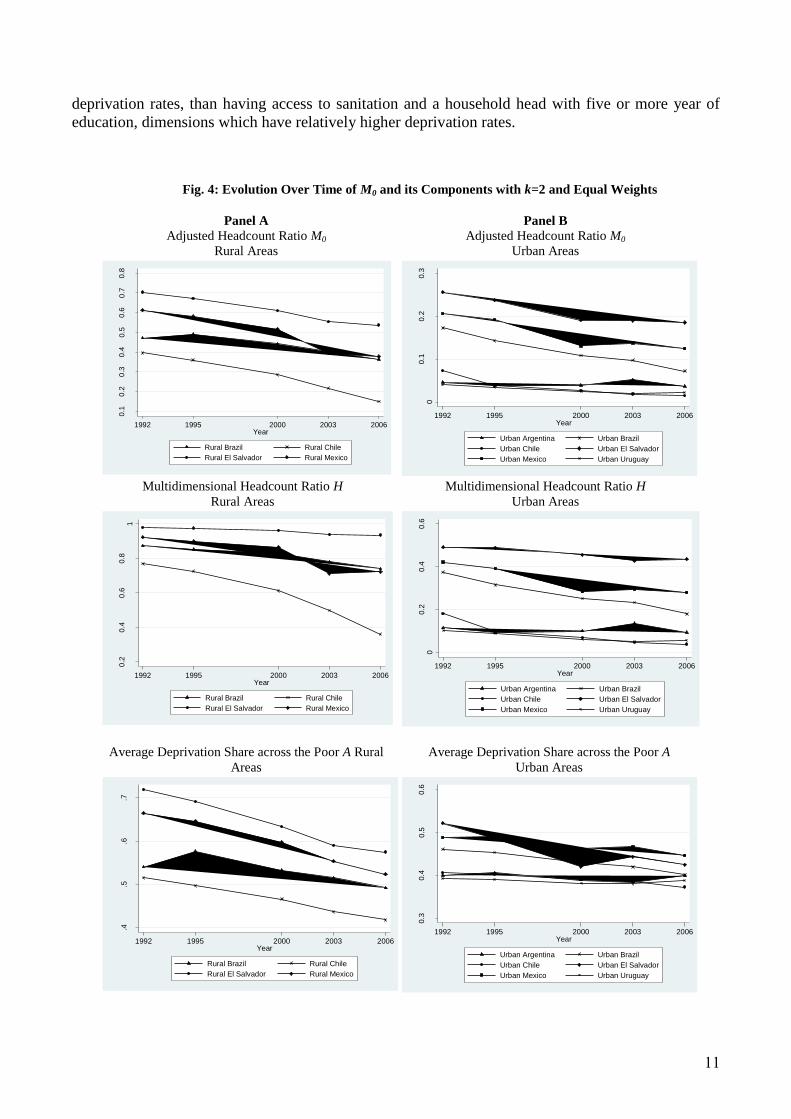
Fig. 4: Evolution Over Time of M0 and its Components with k=2 and Equal Weights
Panel A Panel B
Adjusted Headcount Ratio M0
Rural Areas
Adjusted Headcount Ratio M0
Urban Areas
0.1
0.2
0.3
0.4
0.5
0.6
0.7
0.8
M0
with k
=2
an
d E
qu
al W
eig
ths
1992 1995 2000 2003 2006Year
Rural Brazil Rural Chile
Rural El Salvador Rural Mexico
00.1
0.2
0.3
M0 w
ith
k=
2 a
nd E
qu
al W
eig
ths
1992 1995 2000 2003 2006Year
Urban Argentina Urban Brazil
Urban Chile Urban El Salvador
Urban Mexico Urban Uruguay
Multidimensional Headcount Ratio H
Rural Areas
Multidimensional Headcount Ratio H
Urban Areas
0.2
0.4
0.6
0.8
1
H w
ith k
=2
an
d E
qu
al W
eig
ths
1992 1995 2000 2003 2006Year
Rural Brazil Rural Chile
Rural El Salvador Rural Mexico
00.2
0.4
0.6
H w
ith
k=
2 a
nd E
qu
al W
eig
ths
1992 1995 2000 2003 2006Year
Urban Argentina Urban Brazil
Urban Chile Urban El Salvador
Urban Mexico Urban Uruguay
Average Deprivation Share across the Poor A Rural
Areas
Average Deprivation Share across the Poor A
Urban Areas
.4.5
.6.7
A w
ith
k=
2 a
nd
Eq
ua
l W
eig
ths
1992 1995 2000 2003 2006Year
Rural Brazil Rural Chile
Rural El Salvador Rural Mexico
0.3
0.4
0.5
0.6
A w
ith k
=2
and
Eq
ua
l W
eig
ths
1992 1995 2000 2003 2006Year
Urban Argentina Urban Brazil
Urban Chile Urban El Salvador
Urban Mexico Urban Uruguay
12
Note: It is worth emphasizing that the Adjusted Headcount Ratio M0 (top graph of each panel) is the product of the
Multidimensional Headcount H (middle graph of each panel) and the Average Deprivation Share across the poor A
(bottom graph of each panel).
As explained in the Introduction to this special issue, the M0 measure is the product of two
informative measures: the multidimensional headcount ratio H and the average deprivation share
across the poor A. The evolution of M0 together with its two components H and A over the study
period is presented in Fig. 4 for the case of k=2 and equal weights. Fig. 4 panel A refers to rural areas
of Brazil, Chile, El Salvador and Mexico, while panel B refers to urban areas of these countries
together with Argentina and Uruguay. k=2 is chosen because it is the minimum k that requires an
individual to be deprived in more than one indicator in order to be considered poor (i.e., it is ‘truly’
multidimensional) and at the same time it is meaningful for all countries (for higher k values the
aggregate M0 estimate becomes virtually zero in the urban areas of Chile, Argentina and Uruguay).
This figure shows clearly the different patterns of evolution of multidimensional poverty in rural and
urban areas of the six countries. For example, in both the urban and rural areas of Brazil, Chile, El
Salvador and Mexico, the reduction in M0 is the result both of reductions in the percentage of people
deprived in two or more dimensions (H), as well as of the fact that, on average, they became poor in
fewer dimensions (A). However, the proportional reductions in each of the components of M0 differs
among countries and regions.
One advantage of the M0 measure over the UBN Index and BC measures is that it can be broken
down into the contributions of deprivation in each dimension to overall poverty. Santos et al. (2010)
provide a detailed description of the results of such decomposition for the case of k=2. For this paper
it is worth emphasizing that in all countries deprivation in access to proper sanitation and in the years
of education of the household head are the highest contributors to overall multidimensional poverty –
about a third each. Income deprivation increased its contribution over time in Argentina and
Uruguay, and it is also a significant contributor in Brazil, while in Mexico and Chile, deprivation in
shelter is another significant contributor. What seems encouraging is that deprivation in children
attending school is among the lowest contributors in all countries, which results from the high
enrolment rates observed in the region. This may imply that future generations will enjoy better
educated household heads. These results are consistent with the headcounts by indicator analyzed in
Section 2.1.
3.3 Multidimensional Poverty: BC Family of Measures
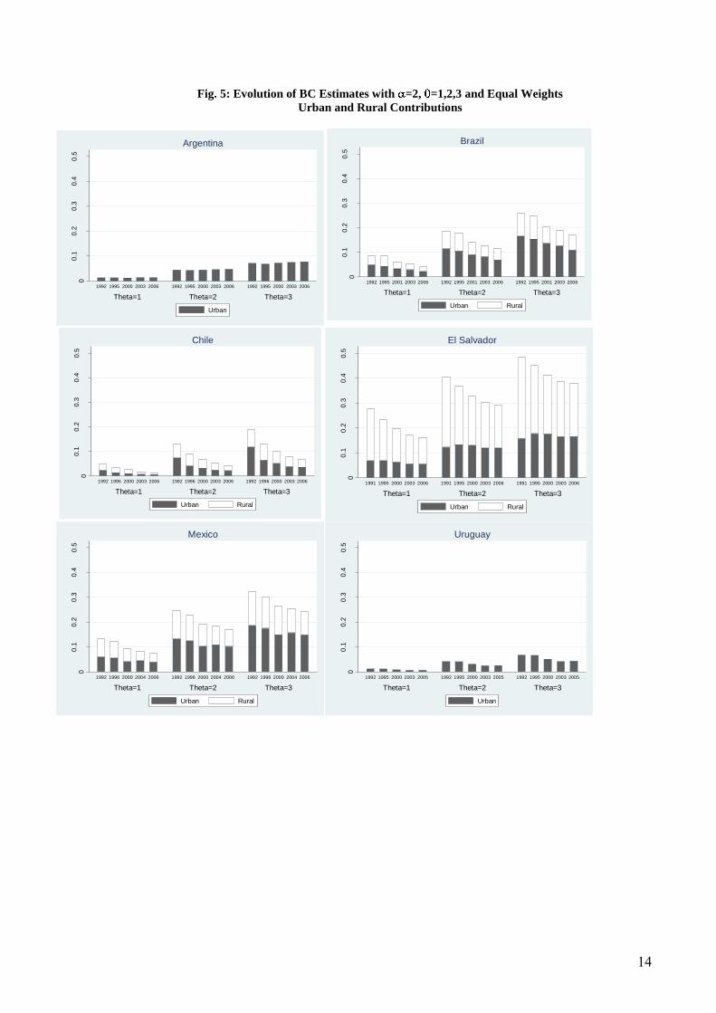
Fig. 5 presents the BC estimates for each country and each year, with 2 and equal weights. It
also contains the contribution of urban and rural areas to the overall estimate. The first group of bars
corresponds to the combination of )1,2( , meaning that dimensions are considered
substitutes, the second group of bars corresponds to the case of )2,2( , which is the M2
measure of AF with k=1, and dimensions are considered independent, and finally the third group of
bars corresponds to the case of )3,2( , with dimensions considered as complements. In all
the figures, results correspond to the equal weights case.17
For a given value of , the estimates of
poverty are higher as increases, as the lower elasticity of substitution, the higher the weight given
in the aggregation to larger gaps.
17 Note that the BC indices with α=0 coincide with the multidimensional headcount for k=1 already reported in Fig. 3. When VP weights are used, the estimates with each combination of (α, θ) are lower. This is because weight is shifted from the dichotomous variables to the two continuous variables that receive the highest weights (income and children in school), which are not the ones with the highest deprivation rates.
13
BC indices with α=1 and α=3, with equal and VP weights were also estimated. Results do not differ
from those emphasized here. The main finding is that for each country over time and across
countries, the same pattern is found across the different values of and , which is in turn
coincident to the one found with the 0M measure. For all combinations of parameters among
countries with information on both urban and rural areas, El Salvador, Mexico and Brazil are the
countries with the highest levels of multidimensional poverty, while Chile is the lowest. In terms of
evolution over time, El Salvador, Mexico, Brazil and Chile experienced important decreases in the
levels of multidimensional poverty for all combinations of parameters. Urban Uruguay experienced a
small reduction in multidimensional poverty, which was already at low levels at the beginning of the
period, while urban Argentina’s estimates remained stable over the study period. The importance of
the results with the BC measures lies in the fact that they imply that both the reduction of
multidimensional poverty found in Brazil, Chile, El Salvador, Mexico and urban Uruguay, as well as
the stagnation found in urban Argentina are robust to the values of the parameters regarding poverty
aversion; in those countries where there was poverty reduction, this was not only in terms of
incidence but also in depth and severity (for the cardinal indicators). Moreover, the results are robust
to alternative assumptions regarding the substitutability, complementarity or independent
relationship between the cardinal indicators.
Independent of the measure used, rural areas have higher poverty than urban ones. However, it is
worth noting that the BC measures allow analysing the change in the ratio of rural to urban poverty
in each country as one alters the balance between the aversion to multidimensional poverty and
aversion to dimension-specific poverty by varying the values of the two parameters α and θ. A higher
value of α gives a higher weight to the multidimensionally poorest individuals whereas a higher
value of θ gives a higher weight to the biggest gaps. In Fig. 6, it can be seen that for a given value of
α, the ratio of rural to urban poverty is decreasing in θ whereas for a given value of θ, it is increasing
in α. These results suggest that more people in rural areas suffer from coupled deprivations, so that
as α is increased, they receive a higher weight and the difference with poverty in urban areas
increases more and more. While people in urban areas experience fewer simultaneous deprivations
than in rural areas, they suffer from poverty gaps at least as big as those in rural areas. When the
poorest gaps receive an increasing weight as θ increases, the difference between poverty in rural and
urban areas is reduced. Therefore, the magnitude of the rural-urban gap depends upon the judgement
on the two types of aversion to poverty.
14
Fig. 5: Evolution of BC Estimates with =2, =1,2,3 and Equal Weights
Urban and Rural Contributions
00.1
0.2
0.3
0.4
0.5
B&
C A
lpha
=2
Theta=1 Theta=2 Theta=3
1992 1995 2000 2003 2006 1992 1995 2000 2003 2006 1992 1995 2000 2003 2006
Argentina
Urban
00
.10
.20
.30
.40
.5
B&
C A
lph
a=
2Theta=1 Theta=2 Theta=3
1992 1995 2001 2003 2006 1992 1995 2001 2003 2006 1992 1995 2001 2003 2006
Brazil
Urban Rural
00
.10
.20
.30
.40
.5
B&
C A
lph
a=
2
Theta=1 Theta=2 Theta=3
1992 1996 2000 2003 2006 1992 1996 2000 2003 2006 1992 1996 2000 2003 2006
Chile
Urban Rural
00
.10
.20
.30
.40
.5
B&
C A
lph
a=
2
Theta=1 Theta=2 Theta=3
1991 1995 2000 2003 2006 1991 1995 2000 2003 2006 1991 1995 2000 2003 2006
El Salvador
Urban Rural
00
.10
.20
.30
.40
.5
B&
C A
lph
a=
2
Theta=1 Theta=2 Theta=3
1992 1996 2000 2004 2006 1992 1996 2000 2004 2006 1992 1996 2000 2004 2006
Mexico
Urban Rural
00
.10
.20
.30
.40
.5
B&
C A
lph
a=
2
Theta=1 Theta=2 Theta=3
1992 1995 2000 2003 2005 1992 1995 2000 2003 2005 1992 1995 2000 2003 2005
Uruguay
Urban

15
Fig. 6: Ratio of Rural Poverty to Urban Poverty BC Estimates
with α=1,2,3, θ=1,2,3 and Equal Weights, 2006
4. Concluding Remarks
This paper provides an in-depth study of multidimensional poverty in Argentina, Brazil, Chile, El
Salvador, Mexico and Uruguay for the period 1992–2006. A hybrid approach is used for the selected
dimensions. They include the widely used income dimension (using the US$2 per day poverty line),
together with five indicators typically considered in the Unsatisfied Basic Needs Approach:
education of the household head (at least five years of education), children attending school, access
to improved sanitation, shelter with adequate wall materials, and access to running water (the latter is
used as the best available proxy for health).
A broad set of measures is estimated, ranging from simple headcounts by indicator and the
multidimensional headcount with different deprivation cut-offs (as typically used by the UBN
approach), to more sophisticated ones which correspond to two multidimensional versions of the
Foster-Greer-Thorbecke class of poverty indices. One of these extensions corresponds to Alkire and
Foster (2007, 2011) which, by assuming that dimensions are independent, allows the measure to be
broken down into the contributions of each dimension (once identification has been applied). The
other extension corresponds to Bourguignon and Chakravarty (2003), which allows for
interrelationships between the dimensions. All estimations were performed for two alternative
weighting systems: one in which each indicator receives the same weight, and another derived from a
participatory study performed in Mexico, where the income and children in school indicators receive
the highest weights (VP weights).
12
34
56
78
91
01
11
21
31
4
Ratio
Rura
l-U
rban
Po
vert
y
1 2 3Theta
Alpha=1 Alpha=2 Alpha=3
Chile
12
34
56
78
91
01
11
21
31
4
Ratio
Rura
l-U
rban
Po
vert
y
1 2 3Theta
Alpha=1 Alpha=2 Alpha=3
Brazil
12
34
56
78
91
01
11
21
31
4
Ratio
Rura
l-U
rban
Po
vert
y
1 2 3Theta
Alpha=1 Alpha=2 Alpha=3
El Salvador
12
34
56
78
91
01
11
21
31
4
Ratio
Rura
l-U
rban
Po
vert
y
1 2 3Theta
Alpha=1 Alpha=2 Alpha=3
Mexico
16
The data available for Brazil, Chile, El Salvador and Mexico allows urban areas to be distinguished
from rural areas. Among these four countries, El Salvador is the poorest, followed by Mexico and
Brazil, while Chile is the least multidimensionally poor. The possibility to distinguish between areas
allows the huge disparities within countries to be identified, to the point that rural areas of Chile can
be grouped together with El Salvador, Mexico and Brazil in terms of their poverty estimates and the
degree of coupled deprivations, while the urban areas of Chile have poverty levels similar to those of
urban Argentina and Uruguay. In El Salvador, Mexico and Brazil, higher poverty and more coupled
disadvantages are found in the rural areas as compared to the urban ones.
Over the study period, El Salvador, Brazil, Mexico and Chile experienced significant reductions of
multidimensional poverty independently of the measure considered. This is a robust result and
suggests that in these countries there was a decrease in the incidence, as well as in the depth and
severity, of multidimensional poverty. An analysis of the components of M0 also showed that the
average number of deprivations among those multidimensionally deprived decreased in the four
countries over the study period. In contrast, in urban Uruguay there was a small reduction in
multidimensional poverty, while in urban Argentina the estimates did not change significantly. Also
contrasting with the other four countries, both Uruguay and Argentina experienced an important
increase in income poverty between 1992 and 2006. However, because of the reduction of
deprivation in other dimensions, this worsening did not translate to an increase in multidimensional
poverty. When VP weights are used, the estimates for all countries tend to be lower, because the two
dimensions that have the highest weight (income and children in school) are not those that show the
highest levels of deprivation. These weights do not significantly change the conclusions regarding
cross-country and over-time comparisons.
These robust results contribute to the discussion of the diversity of experiences in terms of poverty
reduction in the region over the period under study. The years between the early 1990s and the mid-
2000s were especially eventful in Latin America, with a series of structural market-oriented reforms,
the effects of the increasing internationalization and openness of its economies, episodes of growth
and some severe macroeconomic crises. The evidence summarized in the previous paragraph both
complements and reflects these circumstances and trends. The fall in most non-income measures of
deprivation over the whole period indicates a relatively positive outlook, since more structural facets
of poverty seem to have a declining secular trend. Moreover, this trend is especially strong in rural
areas, which have exhibited higher degrees of deprivation over time in the region. The differences
between country-specific trends are also informative: Chile experienced substantial economic growth
over this period, and this is reflected in the downward tendency of all (income and non-income)
measures of deprivation. The results also highlight the economic growth and the vast social
programmes implemented in Brazil and Mexico over the period. Finally, the evidence for Argentina
and Uruguay indicates that non-income measures of deprivation might improve despite mixed
trajectories in terms of income poverty.
This paper opens several lines of debate in terms of policy implications and measures to monitor
poverty in the region. In terms of the measures to monitor poverty, the paper places renewed
attention on the fact that neither the income nor the UBN measures alone are satisfactory. The
evolution of income poverty is sensitive to changes in the flow variable which reacts quickly to crisis
situations. On the other hand, the UBN indicators reflect more structural conditions of poverty, such
as access to basic services, housing and education. These change more slowly, reflecting lagged
effects of policies implemented in the past. Integrating both types of indicators into a single measure
seems relevant and useful. However, a thorough discussion of the dimensions and indicators to
include in a multidimensional poverty measure is needed in the region. Such a discussion is required
to move beyond what data currently offers and to determine whether it is necessary to collect

17
different indicators, ones that – as suggested by the capability approach – capture actual functionings
rather than mere means to them. A further point is the aggregation methodology to be used when
combining such indicators into a multidimensional poverty measure. Whenever the considered
indicators include ordinal variables, which is the most frequent case, it is advisable to use a measure
that is not based on gaps. In such a context, the adjusted headcount ratio M0 is recommended, as it
combines the multidimensional headcount with the average share of deprivations that the poor
experience – making it sensitive to the intensity of poverty.
In terms of policy implications, the paper also refocuses the rural-urban discussion. Many Latin
American countries are now highly urbanised, and this has concentrated resources for poverty
reduction into urban areas. However, our results indicate that poverty is more acute in rural areas.
This calls for policies tailored to these particular regions.
The overall picture from these six Latin American countries seems encouraging, with a decreasing
trend in aggregate multidimensional poverty and in deprivation in the underlying dimensions over
the 1990s and the first half of the 2000s. On the other hand, the international financial crisis of 2007–
2008 and the ensuing fall in prices of commodities exported by countries in the region might hamper
the declining trends in both poverty and inequality in the near future.

18
References
Alkire, S. (2002). Dimensions of human development. World Development, 30 (2), 181-205.
Alkire, S. (2008). Choosing dimensions: The capability approach and multidimensional poverty. In
N. Kakwani & J. Silber (Eds.) The many dimensions of poverty (pp. 89–119). Basingstoke:
Palgrave Macmillan.
Alkire, S. and J. E. Foster (2007), ‘Counting and Multidimensional Poverty Measurement’, OPHI
Working Paper 07, Oxford Poverty & Human Development Initiative.
Alkire, S. and J. E. Foster, (2011) “Counting and multidimensional poverty measurement”, Journal
of Public Economics, 95 (7-8): 476–487.
Alkire, S. and Santos, M. E. (2009). Poverty and inequality measurement. In Deneulin, S. & Shahani,
L. An introduction to the human development and capability approach. (pp 121–161).
London: Earthscan.
Alkire, S. & Santos, M. E. (2010). Acute multidimensional poverty: a new index for developing
countries. OPHI Working Paper No. 38. Oxford: Oxford Poverty and Human Development
Initiative.
Altimir, O. (1982). The extent of poverty in Latin America. World Bank Staff Working Papers No.
522. Washington, DC: World Bank.
Amarante, V., Arim, R. & Vigorito, A. (2010). Multidimensional poverty among children in Uruguay.
Research on Economic Inequality Vol. 18: Studies in Applied Welfare Analysis: Papers from the Third ECINEQ Meeting. Bingley: Emerald, pp: 31 – 253
Arim, R. & Vigorito, A. (2007). Un análisis multidimensional de la pobreza en Uruguay. 1991–2005,
Serie Documentos de Trabajo DT 10/06. Uruguay: Instituto de Economía, Universidad de la
República.
Atkinson, A., Cantillon, B., Marlier, E. & Nolan, B. (2002). Social indicators – The EU and social
inclusion. Oxford: Oxford University Press.
Ballon, P. & Krishnakumar, J. (2008). Estimating basic capabilities: A structural equation model
applied to Bolivia. World Development, 36(6), 992–1010.
Beccaria, L. & Minujin, A. (1985). Metodos Alternativos para Medir la Evolucion del Tamaño de la
Pobreza, Documento de Trabajo No 6. Buenos Aires: INDEC.
Boltvinik, J. (1990). Pobreza y necesidades básicas, conceptos y métodos de medición. Proyecto
Regional para la Superacion de la Pobreza. Caracas: PNUD.
Bourguignon, F. & Chakravarty, S. (2003). The measurement of multidimensional poverty. Journal of
Economic Inequality, 1 (1), 25–49.
CEDLAS (2009). A guide to the SEDLAC-Socio-Economic Database for Latin America and the
Caribbean. Centro de Estudios Distributivos, Laborales y Sociales, Universidad Nacional de La
Plata. http://www.cedlas.org/sedlac.
CEDLAS & World Bank (2009). Socio-Economic Database for Latin America and the Caribbean
(SEDLAC). http://www.cedlas.org/sedlac.
Calvo, C. (2008) Vulnerability to Mulidmensional Poverty. World Development 36, pp. 1011–1020.

19
Chiappero Martinetti E. (2000). A multi-dimensional assessment of well-being based on Sen’s
functioning theory. Rivista Internationale di Scienzie Sociali, CVIII, 207–231.
Conconi, A. & Ham, A. (2007). Pobreza multidimensional relativa: Una aplicación a la Argentina.
Documento de trabajo CEDLAS N. 57. Universidad Nacional de La Plata, Argentina:
CEDLAS.
Cruces, G. & Gasparini, L. (2008). Programas sociales en Argentina: Alternativas para la ampliación
de la cobertura. Documento de trabajo CEDLAS N. 77. Universidad Nacional de La Plata,
Argentina: CEDLAS.
Decancq, K. & Lugo, M. A. forthcoming. Weights in multidimensional indices of well-being: An
overview, Econometrics Review.
Duclos, J-Y., Sahn, D & Younger, S. (2006). Robust multidimensional poverty comparisons. The
Economic Journal, 116 (514), 943–68.
Feres, J. C. & Mancero, X. (2001). El método de las necesidades básicas insatisfechas (NBI) y sus
aplicaciones a América Latina, Series Estudios Estadísticos y Prospectivos. Santiago, Chile:
CEPAL.
Gasparini, L. & Cruces, G. (2008). A distribution in motion: The case of Argentina, Documento de
trabajo CEDLAS N. 78. Universidad Nacional de La Plata, Argentina: CEDLAS.
Gasparini, L., Cruces, G. & Tornarolli, L. (2008). A turning point? Recent developments on inequality
in Latin America and the Caribbean. Nacional de La Plata, Argentina: CEDLAS.
Herrera, A. O., Scolnik, H. D., Chichilnisky, G., Gallopin, G. C., et al. (1976). Catastrophe or new
Society? A Latin America world model. Ottawa: IDRC.
International Labour Organisation. (1976). Meeting basic needs: strategies for eradicating mass
poverty and unemployment : conclusions of the World Employment Conference. Geneva:
ILO.
Betti G., Cheli B., Lemmi A. and Verma V. (2007) The Fuzzy Approach to Multidimensional Poverty:
the Case of Italy in the 1990s, in Kakwani N., Silber J. (eds.), Quantitative Approaches to
Multidimensional Poverty Measurement, Palgrave Macmillan, pp. 30-48.
López-Calva, L. F. & Ortiz-Juárez, E. (2009). Medición multidimensional de la pobreza en México:
significancia estadística en la inclusión de dimensiones no monetarias. Estudios Económicos,
special issue, 3–33.
López-Calva, L. F. & Rodríguez-Chamussy, L. (2005). Muchos rostros, un solo espejo: restricciones
para la medición multidimensional de la pobreza en México. In Székely, M. (Ed.), Números
que mueven al mundo: La medición de la pobreza en México. Mexico City: Miguel Ángel
Porrúa.
Paes de Barros, R., De Carvalho, M. & Franco, S. (2006). Pobreza multidimensional no Brasil. Texto
para discussão No. 1227. Brazil: IPEA.
PNUD (2009) Informe sobre Desarrollo Humano para Mercosur 2009-2010 “Innovar para incluir: jóvenes y desarrollo humano”. Buenos Aires.
Ravallion, M. , Chen, S. and Sangraula, P. (2009) Dollar a Day Revisited. The World Bank Economic
Review 23:163-184.
Santos, M., Lugo, M., Lopez Calva, L. Cruces, G. & Battiston, D. (2010). Refining the basic needs
approach: A multidimensional analysis of poverty in Latin America. Research on Economic
20
Inequality Vol. 18: Studies in Applied Welfare Analysis: Papers from the Third ECINEQ Meeting. Bingley: Emerald, pp: 1 – 29.
Sen, A. (1990). More than 100 million women are missing. New York Review of Books, 20, 61–66.
Sen, A. (1992). Inequality re-examined. Cambridge, MA: Harvard University Press.
Sen, A. K. K. (1999). Development as Freedom, Oxford: Oxford University Press.
Sen, A. (2009). The idea of justice. London: Allen Lane.
Stewart, F. (1980). Country experience in providing for basic needs. In Streeten, P., Stewart, F.,
Burki, S. J., Berg, A., et al. Poverty and basic needs. World Bank Working Paper 33061 (pp.
9–12). Washington, DC: World Bank.
Streeten, P. (1980). From growth to basic needs. In Streeten, P., Stewart, F., Burki, S. J., Berg, A., et
al. Poverty and basic needs. World Bank Working Paper 33061 (pp. 5–8). Washington, DC,
World Bank.
Streeten, P., Burki, J. S., Haq, M. U., Hicks, N. & Stewart, F. (1981). First things first: Meeting basic
human needs in developing countries. New York: Oxford University Press.
Székely, M. (2003). Lo que dicen los pobres. Cuadernos de desarrollo humano No. 13. México:
Secretaría de Desarrollo Social.
The Cocoyoc Declaration. (1974). Adopted by participants in the UNEP/UNCTAD Symposium on
Patterns of Resource Use, Environment and Development Strategies. International
Organization, 29(3), 893–901.
What Now: Another Development. (1976). The 1975 Dag Hammarskjöld report on development and
international cooperation. Sweden: Motala Grafiska.

21
Appendix
Table A.1: Sample size for each country and year, rural and urban areas
Country Household Survey Year Sample Size
(People)
Urban Rural
Argentina*
Encuesta Permanente de Hogares
(EPH)
1992 59,528 NA
1995 62,372 NA
2000 43,255 NA
2003 29,075 NA
Encuesta Permanente de Hogares
Continua (EPH-C)
2006 45,676
NA
Brazil
Pesquisa Nacional por Amostra de
Domicilios (PNAD)
1992 244,473 55,544
1995 266,287 57,859
2001 316,860 52,753
2003 322,839 53,932
2006 337,509 65,372
Chile
Encuesta de Caracterizacion
Socioeconomica Nacional (CASEN)
1992 86,179 46,698
1996 94,925 32,500
2000 142,029 89,441
2003 150,156 80,411
2005 153,234 86,058
El Salvador
Encuesta de Hogares de Propositos
Multiples (EHPM)
1991 49,243 39,235
1995 20,989 18,009
2000 40,940 29,843
2003 35,622 35,708
2005 34,127 35,517
Mexico
Encuesta Nacional de Ingresos y
Gastos de los Hogares (ENIGH)
1992 27,913 20,265
1996 39,974 21,840
2000 26,402 13,989
2004 68,016 21,907
2006 58,760 23,140
Uruguay
Encuesta Continua de Hogares
(ECH)
1992 28,658 NA
1995 64,177 NA
2000 51,913 NA
2003 54,750 NA
2005 53,738 NA
*For the sake of comparability over time, the samples used correspond to the same 15 urban agglomerations.

22
Table A.2: Distribution of the population by number of unmet basic needs and income deprivation status
Rural and Urban Areas, 2006
Urban Rural
%
sample
N° of UBN %
sample
N° of UBN
[0] [1] [2] [3] [4] [5] Total [0] [1] [2] [3] [4] [5] Total
Argentina
Income deprived 9.1 39.6 36.7 17.0 6.1 0.6 0.0 100 - - - - - - - -
Income non-deprived 90.9 78.0 17.9 3.4 0.7 0.0 0.0 100 - - - - - - - -
Brasil
Income deprived 10.6 28.7 35.6 23.8 9.4 2.3 0.2 100 27.0 2.1 11.5 25.1 44.9 14.8 1.5 100
Income non-deprived 89.4 53.9 34.4 9.6 1.8 0.3 0.0 100 73.0 10.2 24.7 35.7 24.1 5.1 0.3 100
Chile
Income deprived 3.0 60.3 28.3 7.5 3.2 0.6 0.0 100 4.5 17.5 25.6 29.1 18.7 8.3 0.8 100
Income non-deprived 97.0 80.9 16.3 2.4 0.3 0.1 0.0 100 95.5 34.5 31.6 21.5 10.2 2.2 0.0 100
Uruguay *
Income deprived 6.0 49.8 29.5 18.0 2.8 0.0 0.0 100 - - - - - - - -
Income non-deprived 94.0 80.8 16.3 2.5 0.4 0.0 0.0 100 - - - - - - - -
Mexico
Income deprived 10.3 17.3 21.5 28.1 22.8 9.7 0.7 100 30.1 3.0 11.5 25.4 35.5 20.2 4.4 100
Income non-deprived 89.7 54.2 24.1 14.2 6.1 1.3 0.1 100 69.9 16.7 21.7 28.5 24.0 8.5 0.6 100
El Salvador *
Income deprived 25.6 14.9 21.1 27.3 22.1 12.1 2.5 100 58.4 0.3 3.9 20.5 30.9 34.5 9.8 100
Income non-deprived 74.4 46.0 24.7 17.6 8.8 2.5 0.3 100 41.6 3.5 11.8 34.0 30.7 17.6 2.4 100
* For these countries, the estimated values correspond to the year 2005
23
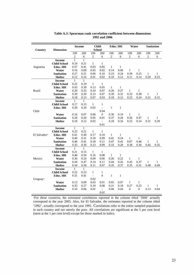
Table A.3: Spearman rank correlation coefficient between dimensions
1992 and 2006
Country
Dimension
Income Child
School
Educ. HH Water Sanitation
199
2
200
6
199
2
200
6
199
2
200
6
199
2
200
6
199
2
200
6
Argentina
Income 1 1
Child School 0.19 0.21 1 1
Educ. HH 0.37 0.41 0.03 0.05 1 1
Water 0.16 0.09 0.05 0.02 0.14 0.06 1 1
Sanitation 0.27 0.31 0.06 0.10 0.23 0.24 0.39 0.25 1 1
Shelter 0.12 0.16 0.01 0.02 0.10 0.12 0.11 0.14 0.20 0.23
Brazil
Income 1 1
Child School 0.22 0.19 1 1
Educ. HH 0.43 0.39 0.13 0.05 1 1
Water 0.29 0.25 0.10 0.07 0.26 0.27 1 1
Sanitation 0.39 0.30 0.13 0.07 0.39 0.32 0.33 0.38 1 1
Shelter 0.18 0.13 0.07 0.03 0.18 0.12 0.23 0.24 0.21 0.15
Chile
Income 1 1
Child School 0.17 0.15 1 1
Educ. HH 0.20 0.29 0.02 -
0.04
1 1
Water 0.16 0.07 0.06 0 0.30 0.19 1 1
Sanitation 0.28 0.20 0.05 0.01 0.37 0.28 0.56 0.47 1 1
Shelter 0.18 0.12 0.02 -
0.01
0.18 0.16 0.25 0.14 0.31 0.28
El Salvador*
Income 1 1
Child School 0.23 0.21 1 1
Educ. HH 0.41 0.40 0.17 0.10 1 1
Water 0.40 0.31 0.19 0.09 0.41 0.24 1 1
Sanitation 0.46 0.41 0.18 0.11 0.47 0.41 0.67 0.46 1 1
Shelter 0.35 0.30 0.13 0.09 0.33 0.28 0.38 0.30 0.45 0.35
Mexico
Income 1 1
Child School 0.21 0.15 1 1
Educ. HH 0.46 0.50 0.16 0.08 1 1
Water 0.30 0.24 0.09 0.06 0.26 0.22 1 1
Sanitation 0.44 0.47 0.14 0.11 0.44 0.43 0.45 0.37 1 1
Shelter 0.34 0.36 0.11 0.07 0.35 0.37 0.35 0.31 0.48 0.49
Uruguay*
Income 1 1
Child School 0.22 0.23 1 1
Educ. HH 0.31 0.41 -
0.02
0 1 1
Water 0.13 0.09 0.03 0.01 0.05 0.07 1 1
Sanitation 0.35 0.27 0.10 0.08 0.21 0.18 0.27 0.25 1 1
Shelter 0.10 0.06 0.01 -
0.01
0.06 0.04 0 0 0.13 0.04
*For these countries, the estimated correlations reported in the column titled ‘2006’ actually
correspond to the year 2005. Also, for El Salvador, the estimates reported in the column titled
‘1992’, actually correspond to the year 1991. Correlations refer to the entire sampled population
in each country and not merely the poor. All correlations are significant at the 5 per cent level
(most at the 1 per cent level) except for those marked in italics.