Counterparty Credit Risk in Interest RateSwaps during Times of Market Stress

Antulio N. Bomfim∗

Federal Reserve Board

First Draft: September 27, 2002

This Draft: December 17, 2002

Abstract

This paper examines whether empirical and theoretical results sug-gesting a relatively small role for counterparty credit risk in the deter-mination of interest rate swap rates hold during periods of stress in thefinancial markets, such as the chain of events that followed the Rus-sian default crisis of 1998. The analysis sheds light on the robustnessof netting and credit enhancement mechanisms, which are common ininterest rate swaps, to widespread turmoil in the financial markets.

JEL Classification: G12, G13

Keywords: convexity adjustment, futures and forward rates, affine models

∗Board of Governors of the Federal Reserve System, Washington, DC 20551; E-mail:abomfim@frb.gov; Fax: (202) 452-2301, Tel.: (202) 736-5619. I am grateful to JeffDewynne and Pat White for helpful comments, to Emily Cauble and Joseph Rosenbergfor excellent research assistance, and to seminar participants at the Federal Reserve Boardfor their insights. The opinions expressed in this paper are not necessarily shared by theBoard of Governors of the Federal Reserve System or any other members of its staff.

1 Introduction

Spreads of rates on interest rate swaps over comparable U.S. Treasury yields

widened dramatically during the acute financial market turmoil that followed

the Russian default crisis of 1998 (Figure 1). While a significant portion of

that widening in swap spreads likely reflected increased concerns about credit

risk in general and greater demand by investors for the safety and liquidity

of Treasury securities—corporate bond and LIBOR spreads over Treasuries

had also moved substantially higher—it is conceivable that swap spreads were

also affected by market participants’ worries about counterparty credit risk in

swaps. This paper examines a well-known no-arbitrage relationship between

interest rate swaps and eurodollar futures contracts to take a novel look at

this issue. In particular, I examine whether the spread between swap rates

quoted by dealers and “synthetic” swap rates implied by the futures market—

where counterparty credit risk is virtually absent—provided any indication

that swap rates were signaling heightened concerns about counterparty risk

in the swaps market at that time.

Understanding the potential role that concerns about counterparty credit

risk play in the pricing of interest rate swaps during times of financial mar-

ket stress is important for at least two reasons. First, while a vast academic

literature has studied the issue both from a theoretical and an empirical per-

spective, existing studies have not assessed the robustness of their findings to

episodes of turmoil in the financial markets. Second, the interest swap mar-

ket has been increasingly taking on a benchmark role in the broader fixed-

income market that had previously virtually been the exclusive domain of

U.S. Treasury debt securities. Given its greater prominence for the financial

markets as a whole, the question of assessing the ability of the swaps mar-

ket to continue to function without major impediments—such as heightened

concerns about counterparty credit risk—when other (less liquid) markets

are disrupted gains special significance for academics, market practitioners,

1

and policymakers alike.

This paper is organized as follows. In Section 2, I provide some back-

ground on the institutional make-up of the interest rate swap market, as

well as the theoretical underpinnings of swap valuation. Section 3 contains

a review of the literature on counterparty credit risk in swaps, and, in Sec-

tion 4, I discuss the construction of synthetic swap rates from futures rates,

including a discussion of the modeling framework used to estimate the con-

vexity differential between futures and forward rates. In Section 5, I describe

how synthetic swap rates were constructed in practice. I conduct formal

statistical comparisons between market and synthetic swap rates in Section

6, examining the potential role of counterparty credit risk in the pricing of

swaps in general and during times of market stress in particular. Section

7 includes an assessment of the robustness of the main results to different

modeling assumptions in the derivation of the convexity adjustment, and,

in Section 8, I discuss alternative interpretations of the findings. Section 9

contains an overall summary and the main conclusions.

2 Interest Rate Swaps

In its most common (vanilla) form, an interest rate swap is an agreement

between two parties to exchange fixed and variable interest rate payments

on a notional principal amount over a predetermined period ranging from one

to thirty years. The notional amount itself is never exchanged. In the United

States, the variable interest rate is typically six- or three-month LIBOR, and

the fixed interest rate, which is determined in the swaps market, is generally

quoted as a spread to yields on recently auctioned Treasury securities of

comparable maturity.

The overall credit quality of swap market participants is high, commonly

rated A or above; those entities with credit ratings of BBB or lower are

typically either rejected or required to adopt stricter credit enhancing mech-

2

anisms, which are clauses in swap agreements that are intended to mitigate

concerns about counterparty credit risk in swaps. Such mechanisms include

(i) credit triggers clauses, which give the higher-quality counterparty the

right to terminate the swap if its counterparty’s credit rating falls below,

say, BBB, (ii) the posting of collateral against the market value of the swap,

and (iii) requirements to obtain insurance or guarantees from highly-rated

third parties (Litzenberger, 1992).

Swaps are negotiated and traded in a large over-the-counter market that

has grown spectacularly since its inception in the early 1980s. According to

the Bank for International Settlements (2002), notional amounts outstand-

ing in U.S. dollar-denominated swaps reached $19 trillion at the end of 2001.

Most swaps are entered with dealers, who then seek to limit their exposure

to interest rate risk by entering into offsetting swaps with other counter-

parties. In addition to swap dealers, major market participants include fi-

nancial institutions and other corporations, international organizations such

as the World Bank, government-sponsored enterprises, corporate bond and

mortgage-backed securities dealers, and hedge funds.

The swap market is one of the most active segments of the global fixed-

income market. The introduction, in the mid-1980s, of master swap agree-

ments, which are standardized legally binding agreements that detail the

rights and obligations of each party in the swap, helped enhance market liq-

uidity. Rather than spending time and resources on bilateral negotiations

on the terms and language of individual contracts, such master agreements,

which were sponsored by ISDA—the International Swaps and Derivatives

Association—allowed market participants to converge to a common set of

market practices and standards. Attesting to the liquidity of the market,

typical bid-asked spreads are substantially narrower for swaps than those

corresponding to even the most liquid corporate bonds.

As the swap market has grown in size and liquidity, so have dealers’

exposures to each other and, in response, the practice of posting collateral

3

that can be used to limit potential default-related losses in swaps has become

increasingly widespread even among major market participants, as opposed

to being limited to agreements with counterparties of lower credit quality.

Also widespread, indeed virtually universal, is the practice of netting, which

means that, rather than exchanging fixed and floating payments on the dates

specified in the swap contract, the values of the two payments are netted,

and only the party with a net amount due transfers funds to its counterparty.

2.1 Swap valuation

Consider an interest rate swap entered at time-t, with simultaneous ex-

changes of payments at dates Si, i = 1, ..., n, and a notional amount of $1.

Let Y (t, Sn) denote the fixed rate written into the swap agreement, expressed

on an annual basis. The floating-rate payments are assumed to be LIBOR

flat so that, at each payment date Si, the fixed-rate receiver pays δiL(Si−1, Si)

to its swap counterparty and receives in return the amount δiY (t, Sn), where

δi is the accrual factor that pertains to period [Si, Si+1]—e.g., if the swap in-

volves semiannual payments, δi = 0.5—and L(Si−1, Si) is the corresponding

LIBOR, also expressed on an annual basis.1

A simple approach to value such a swap is to compute the market values

of its fixed- and floating-rate payments separately. For a fixed-rate receiver,

the market value V (SWA)(t, S) of the swap is the difference between the time-

t market value of the fixed leg, V (FX)(t, S), and that of the floating leg,

V (FL)(t, S), where S ≡ [S1, S2, ..., Sn].

Assuming that there is no risk that either party in the swap will renege on

its obligations, i.e. there is no counterparty credit risk, the valuation of the

floating and fixed legs of the swap is relatively straightforward. In particular,

1For ease of exposition, I ignore the different day-count conventions of the money andbond markets, which would affect the accrual factors used in the evaluation of the fixedand floating legs of the swap. These conventions, however, are explicitly taken into accountin the empirical work described in later sections.

4

I assume that the future payments associated with both legs are discounted

based on the same zero-coupon yield curve, with no adjustment for the credit

quality of individual counterparties. For the fixed leg I can write

V (FX)(t, S) =n∑

i=1

δiY (t, Sn)P (t, Si) (1)

where P (t, Si) is the time-t price of a zero-coupon bond that matures at Si,

which is the time-t value of $1 to be received at Si.

To value the floating leg of the swap, I rely on a simple investment strategy

that exactly replicates its cash flow: At time t an investor sells a zero-coupon

bond that matures at Sn and invests $1 into a LIBOR-paying bank account,

for a net cash outlay of 1 − P (t, Sn). The bond has a face value of $1, and

the bank deposit pays an interest rate of L(t, S1) per annum, where S1 is

the maturity date of the deposit and L(t, S1) has a compounding frequency

of δ1 ≡ S1 − t. At time S1, the investor receives 1 + δ1L(t, S1) from the

bank, reinvests $1 into another LIBOR-paying deposit, this one maturing at

S2 and paying the interest rate L(S1, S2), and ends up with a net cash flow

of δ1L(t, S1). The investors keeps on following this same strategy at times

Si, i = 2, ..., n− 1, receiving a net payment of δiL(Si−1, Si) in each occasion.

Lastly, at time Sn, the investor receives 1 + δnL(Sn−1, Sn) from the bank,

pays back the face value of the bond issued at t, receiving a net cash flow of

δnL(Sn−1, Sn).

Note that the cash flow of the above investment strategy matches exactly

the floating-rate payments of the swap. As a result, in the absence of arbi-

trage opportunities, the time-t value of the swap’s floating leg should then

be equal to the time-t cash outlay of the investment strategy. Thus,

V (FL)(t, S) = 1 − P (t, Sn) (2)

5

which implies that the time-t value of the swap for a fixed-rate receiver is

V (SWA)(t, S) =n∑

i=1

δiY (t, Sn)P (t, Si) − 1 + P (t, Sn) (3)

2.2 Par swap rates and forward rates

It typically costs nothing to enter into a vanilla swap, which implies that the

swap rate written into the contract is such that the swap has zero market

value at its inception. Solving (3) for Y (t, Sn) while setting V (SWA)(t, S) = 0,

I obtain the following expression for the “par” swap rate Y ∗(t, Sn)

Y ∗(t, Sn) =1 − P (t, Sn)∑ni=1 δiP (t, Si)

(4)

For the purposes of this paper, it will be convenient to express P (t, Si) in

terms of simple (discretely compounded) forward rates. It can be shown that

the time-t forward LIBOR that corresponds to the future period [Si−1, Si] can

be written as

h(t, Si−1, Si) = δ−1i

[P (t, Si−1)

P (t, Si)− 1

](5)

Note that, starting with i = 1—and defining S0 ≡ t—I can solve (5)

recursively to write zero-coupon bond prices in terms of simple forward rates.

This allows me to express par swap rates entirely as a function of the forward

LIBOR curve, h(t, Sj−1, Sj), j = 1, 2, ..., n,

Y ∗(t, Sn) =1 − ∏n

j=1[1 + δjh(t, Sj−1, Sj)]−1∑n

i=1

∏ij=1[1 + δjh(t, Sj−1, Sj)]−1

(6)

Equation (6), which is a model-independent relationship, plays a central

role in the reminder of this paper. It implies that, for a given position of the

forward LIBOR curve, one can synthesize par swap rates, which, in the ab-

sence of arbitrage opportunities and liquidity and credit-quality differentials

6

between the swap and forward LIBOR markets, should correspond to the

swap rates quoted in the marketplace. Hence, under the market conditions

just described, one can think of (6) as the fair value of the par swap rate.

3 Counterparty Credit Risk in Swaps

In the previous section, I made two main simplifying assumptions to outline

a simple methodology for determining the fair market value of an interest

rate swap. First, I assumed the absence of counterparty credit risk in the

derivation of the expression for the par swap rate. Second, in establishing

a link between swaps and the forward LIBOR curve, I assumed that the

two corresponding markets are equally liquid across all maturities. In this

section, I shall assess the likely consequences of relaxing the first of these

assumptions by examining theoretical and empirical results regarding the

importance of counterparty credit risk in the determination of swap rates. I

shall turn to the second assumption in the next section.

There is a vast literature in which counterparty credit risk in swaps is

examined, with some studies dating back to the early years of the market.

For instance, Cooper and Mello (1991) used a partial equilibrium framework

to model the default risk premium embedded in swap rates and found that,

although uncollateralized swaps do entail some counterparty credit risk expo-

sure, such an exposure is substantially lower than that in related debt market

instruments such as fixed- and floating-rate notes. In particular, given the

netting provisions of swap contracts (discussed in Section 2), the counter-

parties are exposed only to the net difference between cash flows on the two

synthetic debt contracts underlying the swap.

Another relatively early work on the importance of counterparty risk in

swaps is that of Sorensen and Bollier (1994), who used an option theoretic

framework that explicitly took into account both bilateral risk—or the fact

that counterparties are exposed to each other’s credit risk—and the effects of

7

the slope of the yield curve on the determination of swap rates. They found

that, when the yield curve steepens because of greater odds of higher interest

rates in the future, the market value of fixed-rate paying positions in swaps

becomes more likely to rise than to fall, leaving the holders of such positions

more exposed to their swap counterparties, the floating-rate payers. (The

reverse would be true in a flattening yield curve environment.) Sorensen and

Bollier (1994) reported that adjustments to swap rates because of the credit

risk of the counterparty can range from less than one basis point to more than

15 basis, but adjustments in excess of 10 basis points corresponded to swaps

arranged with speculative-grade firms—who are not typical counterparties in

swaps—under the most unfavorable term structure environments.

In practice, the role of counterparty credit risk in the determination of

swap rates could be even lower than the relatively small effects suggested

by Cooper and Mello (1991) and Sorensen and Bollier (1994). In particular,

their analyses did not consider some important institutional details of the

market, many of which are specifically designed to address issues related to

the creditworthiness of potential counterparties. Such institutional details

are at the heart of the discussion by Litzenberger (1992), who argued that

swap dealers typically do not vary quoted swap rates with the credit quality of

the prospective counterparty, instead adopting the practice of either rejecting

counterparties with weaker credit ratings or requiring them to adopt one or

more of the credit enhancement techniques described in Section 2.

More recent theoretical work has tended to confirm Litzenberger’s main

conclusions. For instance, Duffie and Huang (1996) proposed a model of

asymmetric default risk that takes into account both the default character-

istics of the counterparties and the probability distribution of the potential

paths taken by the future value of the swap itself. The latter issue was not

examined explicitly by Sorensen and Bollier (1994), and Duffie and Huang

found even smaller effects of counterparty credit risk on swap rates than did

Sorensen and Bollier. They reported that swap spreads are virtually insen-

8

sitive to the credit quality of the counterparties, a result that, similar to the

above mentioned paper by Cooper and Mello (1991), depended importantly

on the netting provisions of swap contracts. Huge and Lando (1999) ex-

tended the Duffie-Huang framework to explicitly take into account the credit

rating of each counterparty and to allow additional credit enhancement mech-

anisms in swap agreements, such as credit triggers. Their theoretical work,

too, found little scope for counterparty credit risk to affect swap rates, and,

indeed, recent papers on the determinants of swap rates abstract from credit

risk questions altogether (e.g., He, 2000 and Liu, Longstaff, and Mandell,

2002).

Nonetheless, Minton (1997) interpreted results of her empirical analysis

of swap rates as casting some doubt on Litzenberger’s main conclusions and

on the theoretical results obtained by Duffie and Huang and others. Using

futures rates as proxies for forward rates, she used the methodology described

in Section 2 to construct swap rates implied by the no-arbitrage relationship

between swaps and forward rates. She found that (6) failed to hold in her

sample. She then reported on evidence that suggested that proxies for con-

cerns about counterparty credit risk—such as spreads between yields on cor-

porate bonds and those on U.S. Treasury securities—played, in some cases, a

statistically significant role in the determination of swap rates. In particular,

Minton argued that the fact that actual swap rates differ from those implied

by the futures market—where the futures exchange and margining provi-

sions essentially eliminate worries about counterparty credit risk—could be

interpreted as a sign of counterparty risk concerns in the interest rate swap

market.

More recently, however, Gupta and Subrahmanyam (2000) provided some

counter evidence to Minton’s findings. Although Gupta and Subrahmanyam’s

focus was on whether interest rate swaps were correctly priced in the early

years of the swap market, they also examined the relationship between swap

rates and proxies for counterparty credit risk similar to the ones used by

9

Minton. They found that, while statistically significant in some instances,

the effect of counterparty risk on swap rates is so small as to be economically

insignificant. Gupta and Subrahmanyam also argued that Minton’s approach

of using futures as direct proxies for forward rates introduces a significant

bias in the pricing of interest rate swaps because such a practice ignores the

differential convexity of the two contracts.2 Accordingly, they used various

interest rate models to derive a convexity adjustment for futures rates (rela-

tive to forward rates) and argued that the spread between actual swap rates

and those implied by unadjusted futures rates moves largely in line with the

convexity adjustment term and not, as suggested by Minton, as a result of

counterparty credit risk.

Minton’s (1997) and Gupta and Subrahamanyam’s (2000) work, as well

as most of the empirical papers referenced above, predate recent episodes of

stress in financial markets, ranging from the Asian financial crisis of 1997

to the bout of financial market uncertainty surrounding the century-date

change.3 Thus, the question of whether credit enhancement mechanisms and

netting arrangements have been sufficiently effective in insulating swap rates

from concerns about counterparty risk during times of turmoil in the broader

financial markets remains largely unanswered. Addressing this empirical is-

sue is one of the main intended contributions of this paper. I extend the

empirical analysis of Minton (1997) and Gupta and Subrahmanyam (2000)

by examining the likely importance of concerns about counterparty credit

risk in the determination of swap rates in a larger and more recent sample

and, more important, in a framework that explicitly allows for such concerns

to potentially play a more prominent role during times of financial market

2In addition to Gupta and Subrahmanyam (2000), the relationship between forwardand futures contracts has been analyzed in several previous works, including Cox, Ingersoll,and Ross (1981), Sundaresan (1991), Burghardt, Belton, Lane, Luce, and McVey (1991),Kamara (1994), Muelbroek (1992), and Grinblatt and Jegadeesh (1996). The next sectiondiscusses the convexity adjustment factor in some detail.

3Gupta and Subrahmanyam (2000) used data through 1996.

10

stress.4

4 Futures-Implied Swap Rates

I now turn to the other main simplifying assumption implicitly made in

Section 2, the one that asserted that the forward LIBOR quotes in the right-

hand-side of (6) were derived from a market that is as liquid as that for

interest rate swaps. In reality, liquidity in the LIBOR market is highly con-

centrated in instruments maturing in less than two years, and the same is

true for the forward rate agreement market, where forward LIBOR contracts

are commonly negotiated. As a result, assessing the no-arbitrage relationship

between par swap rates and the forward LIBOR curve is not as simple as

(6) suggests. Instead of directly relying on (6), many market practitioners

and researchers have often turned to eurodollar futures contracts, which are

highly liquid close cousins to forward LIBOR contracts, to determine fair

valuations and potentially identify mispricings across the LIBOR and swap

markets.

4.1 Anatomy of an eurodollar futures contract

At its core, an eurodollar futures contract is very similar to a forward LIBOR

contract. Let H(t, Si−1, Si) be the time-t annualized interest rate written into

a newly entered futures contract, where the interest rate will be applied to a

future period [Si−1, Si], and I assume that the notional amount of the contract

is $1. In principle, similar to a forward contract, one of the parties to the

futures contract has agreed to borrow $1 at time Si−1 and repay it at time Si

plus an interest payment of δiH(t, Si−1, Si). Also analogous to most forward

4Other papers that address the issue of counterparty credit risk in swaps include Belton(1987), Sun, Sundaresan, and Wang (1993), Duffie and Singleton (1997), and Grinblatt(2001).

11

LIBOR contracts, the rate H(t, Si−1, Si) is such that the futures contract has

zero market value at its inception, in which case H(t, Si−1, Si) is called the

time-t futures rate for future lending/borrowing at [Si−1, Si].5

In the United States, eurodollar futures contracts are traded primarily at

the Chicago Mercantile Exchange (CME), with the maturity of the underly-

ing futures rates, Si − Si−1, most commonly corresponding to three months.

As for the maturities of the contracts themselves, Si−1− t, they range from a

few days to as far out as ten years. Eurodollar futures contracts are among

the most liquid futures contracts traded in the CME and the Chicago Board

of Trade, the two major futures exchanges in the United States.

Combined with their high liquidity, the close resemblance between futures

and forward contracts, makes eurodollar futures rates potentially useful prox-

ies for the forward LIBOR rates that appeared in equation (6). Nonetheless,

futures and forward contracts do differ in a subtle but important way: Fu-

tures contracts are marked to market on a daily basis and, unlike a forward

contract—which pays out only at its maturity—margin account balances are

adjusted accordingly throughout the life of the futures contract. This dif-

ference in the timing of cash flows associated with the two contracts has

important implications for their pricing.

4.2 Futures and forward rates in a generic spot rate

model

All the results that I have derived thus far are model independent. To take a

closer look at the difference between futures and forward rates, and the im-

plications of using the former in the no-arbitrage relationship between swap

and forward rates—equation (6)—I will now turn to a relatively simple mod-

eling framework that is general enough to encompass a variety of well-known

spot interest rate models. In particular, I start by assuming that forward

5Throughout this paper, I assume the equality between lending and borrowing rates.

12

and futures rates are functions f(r(t), t, Si−1, Si) and F (r(t), t, Si−1, Si), re-

spectively, of the spot rate r(t)—defined as the instantaneous short rate at

time t—where the specific forms of f(.) and F (.) are yet to be determined.

Regarding r(t), I assume that it follows a stochastic process with drift

µ(r, t) and diffusion v(r, t) under the real (objective) probability measure.

dr(t) = µ(r, t)dt + v(r, t)dX(t) (7)

and where dX(t) is an infinitesimal increment in a standard Brownian motion

under the objective measure. I shall refer to (7) as a generic spot rate model

for as long as I leave the functional forms of µ(r, t) and v(r, t) unspecified.

Futures contracts. To derive an expression for the futures rate under the

generic spot rate model, I follow a valuation approach similar to the Black-

Scholes methodology for valuing calls and puts. This allows me to write

down the partial differential equation that F (.) must satisfy in an economy

without arbitrage opportunities:

∂F

∂t+

v(r, t)2

2

∂2F

∂r2+ [µ(r, t) − λ(r, t)v(r, t)]

∂F

∂r= 0 (8)

where λ(.) denotes the market price of risk. The final condition given by

F (r(Si−1), Si−1, Si−1, Si) = L(Si−1, Si) (9)

i.e., the futures rate must converge to the spot rate.

At this point, I can invoke the Feynman-Kac stochastic representation

formula to obtain the function F (.) that solves the problem defined by (8)

and (9):

F (r(t), t, Si−1, Si) = Et[L(Si−1, Si)] (10)

where Et[.] denotes an expectation based on the risk-adjusted (risk-neutral)

13

process for r(t):

dr(t) = [µ(r, t) − λ(r, t)v(r, t)] dt + v(r, t)dX(t) (11)

and where dX(t) is an infinitesimal increment in a standard Brownian motion

under the risk-neutral measure.

Equation (10) is the familiar result that the futures rate corresponds to

the risk-adjusted expectation of the interest rate underlying the contract.

Forward contracts. The derivation of the forward LIBOR curve in the context

of the spot rate model is straightforward. Consider a forward LIBOR contract

written at time t for borrowing $1 at the future period [Si−1, Si]. The contract

will be cash-settled at time Si−1 and its payoff will be based on the difference

between the L(Si−1, Si)—the actual LIBOR prevailing at Si−1 for lending

and borrowing until Si—and the rate K∗ specified in the contract.6 I can

use the risk-neutral valuation approach to write out the time-t value of this

forward contract

V (FWD)(r(t), t, Si−1, Si) = Et{e−R Si−1

t r(s)dsδi[L(Si−1, Si) − K∗]} (12)

where, as above, Et[.] denotes a conditional expectation computed under the

risk-neutral probability measure.

Equation (12) has the intuitive result that the market value of the forward

contract is just the risk-adjusted expectation of the present value of its payoff.

Ordinarily, of course, it costs nothing to enter into a forward contract so that,

in the absence of arbitrage opportunities, the rate K∗ specified in the contract

is such that V (FWD)(r(t), t, Si−1, Si) = 0. Letting f(r(t), t, Si−1, Si) denote

6This is basically the structure of a forward rate agreement (FRA), which is a commonlynegotiated over-the-counter contract.

14

the value of K∗ such that V (FWD)(r(t), t, Si−1, Si) = 0, I obtain

f(r(t), t, Si−1, Si) =Et[e

− R Si−1t r(s)dsL(Si−1, Si)]

Et[e−R Si−1t r(s)ds]

(13)

which is the function that the forward LIBOR curve satisfies in the generic

spot rate model.

The futures-forward differential. I am now ready to compare futures and

forward rates in the context of the generic spot rate model. Using the fact

that, for any two stochastic variables zi and zj , Et[zizj ] = Et[zi]Et[zj] +

cvt[zi, zj], where cvt[zi, zj] denotes the covariance of zi and zj under the risk

neutral measure, I can rewrite (13) as

f(r(t), t, Si−1, Si) = F (r(t), t, Si−1, Si) +cvt[e

− R Si−1t r(s)ds, L(Si−1, Si)]

Et[e−R Si−1t r(s)ds]

(14)

where, to arrive at the above expression, I used (10).

Note that the last term of the above equation is the so-called convexity

adjustment that translates futures rates into forward rates. When the short

rate is deterministic, the covariance term is zero and forward and futures

rates coincide, as demonstrated by Cox, Ingersoll, and Ross (1981) and many

others.

4.3 Results from a specific spot rate model

One can write out an explicit formula for the difference between futures and

forward rates by making specific assumptions about the drift and diffusion

terms of the generic spot rate model (11). I show below how this can be done

with the no-arbitrage model of Ho and Lee (1986). The Ho-Lee model has

the advantage that it is extremely simple and tractable, and this is my main

motivation for using it in this illustrative subsection. Its simplicity, however,

15

comes at the cost of some unrealistic implications, discussed in Section 7,

where I also examine results based on other models.

In the Ho-Lee model, the drift and the diffusion terms of the risk-neutral

process for r(t), (11), become µ(r, t) − λ(r, t)v(r, t) = θ(t) and v(r, t) = σ,

where σ denotes the volatility of the short rate, and the drift θ(t) is chosen

at each point in time such that the theoretical bond prices implied by the

model fit the observed term structure of interest rates exactly.

Using a standard hedging argument, one can show that the time-t price

P (r(t), t, S) of a zero-coupon bond maturing at time S satisfies the following

partial differential equation

∂P

∂t+

σ2

2

∂2P

∂r2+ θ

∂P

∂r− rP = 0 (15)

with final condition given by P (r(S), S, S) = 1. The solution to this PDE

has the form

P (r(t), t, S) = e−A(t,S)−B(t,S)r(t) (16)

where B(t, S) ≡ S − t and A(t, S) ≡ ∫ S

tθ(s)[s − S]ds + σ2[S−t]3

6, and, to

ensure that the model fits observed bond prices exactly, θ(s) = ∂f∗(t,s)∂s

+

σ2[s− t], where f ∗(t, s) denotes the instantaneous time-t forward for lending

or borrowing at time s, for s > t, derived directly from observed market

prices.

In light of (5) and (16), the simple time-t forward rate that corresponds

to the future period [Si−1, Si] can be written as:

f(r(t), t, Si−1, Si) =1

δi

[eA(Si−1,Si)+B(Si−1,Si)Et[r(Si−1)]−σ2

2p(t,Si−1,Si) − 1

](17)

where p(t, Si−1, Si) ≡ (Si−1 − t)(Si − t)(Si − Si−1), and, given (11) and θ(t),

Et[r(Si−1)] = r(t) +

∫ Si−1

t

θ(s)ds = f ∗(t, Si−1) +σ2

2(Si−1 − t)2

16

In the Ho-Lee model, the futures rate F (t, Si−1, Si) becomes

F (r(t), t, Si−1, Si) =1

δi

[eA(Si−1,Si)+B(Si−1,Si)Et[r(Si−1)]+

12Vt[r(Si−1)]B(Si−1,Si)2 − 1

](18)

where Vt[r(Si−1)] ≡ σ2(Si−1 − t) denotes the conditional variance of r(Si−1),

computed under the risk-neutral measure, based on information available at

time t.

From equations (17) and (18) I can derive the convexity adjustment,

ξ(r(t), t, Si−1, Si) ≡ F (r(t), t, Si−1, Si) − f(r(t), t, Si−1, Si), that converts ob-

served eurodollar futures rates into implied forward rates,

ξ(r(t), t, Si−1, Si) = q(r(t), t, Si−1, Si)[1 − e−

σ2

2(Si−1−t)(Si−Si−1)[(Si−1−t)+2(Si−Si−1)]

](19)

where q(r(t), t, Si−1, Si) ≡ F (r(t), t, Si−1, Si) + δ−1i . It can be shown that the

convexity adjustment is positive and that it is an increasing function both of

the volatility σ of the short rate and of the maturity (Si−1 − t) of the futures

contract.7 Thus, for instance, the longer the maturity of a futures contract,

the more its corresponding futures rate will overstate the forward rate that

pertains to a forward contract of same maturity.

The results obtained thus far allow us to use the Ho-Lee model to translate

futures rates into forward rates and, in light of (6), obtain the corresponding

futures-implied par swap rate:

Y (t, Sn) =1 − ∏n

j=1[1 + δj f(r(t), t, Sj−1, Sj)]−1∑n

i=1

∏ij=1[1 + δj f(r(t), t, Sj−1, Sj)]−1

(20)

where I used the symbols Y (.) and f(.) to denote model-dependent futures-

implied par swap and forward rates, respectively, as opposed to the symbols

7ξ(r(t), t, Si−1, Si) is also increasing in (S2−S1), the maturity of the underlying LIBORdeposit, but this relationship is less important for my purposes given my focus on contractswritten on three-month LIBOR.

17

Y ∗(.) and f(.), which I used to represent observed par swap rates and the

forward rates that would prevail in a fully liquid forward LIBOR market.

I shall henceforth refer to Y (t, Sn) as the synthetic swap rate. As demon-

strated above, such a rate is jointly determined by the eurodollar futures

curve and the particular spot rate model used to compute the convexity

adjustment. To check the sensitivity of my empirical findings to the as-

sumptions made in the Ho-Lee model, I shall follow the spirit of Gupta and

Subrahmanyam (2000) and report results for a variety of well-known interest

rate models.

5 Synthetic Swap Rates

I now take the theoretical results derived in earlier sections and apply them

to the data in order to examine whether they were valid over the past decade,

in general, and during times of market stress in particular. Again, the basic

premise of the analysis is that I can use synthetic swap rates computed

from convexity-adjusted futures rates as benchmark swap rates involving no

adjustment for counterparty credit risk, as this is absent in the exchange-

based futures market. Given these synthetic rates, I examine the extent to

which they differ from actual swap rates and whether such differences can

be explained by common proxies for counterparty credit risk. I use weekly

quotes on one-, three-, and six-month LIBOR, two-, three-, five-, seven-,

and ten-year swap rates, three-month eurodollar futures rates for contract

maturities extending through ten years, and prices of European options to

enter into five-year swaps (swaptions), with expiration dates ranging from

six months to five years. The data are sampled from quotes which extend

from January 1994 to March 2002.

18

5.1 Futures-implied swap rates

The first step in the construction of swap rates implied by eurodollar fu-

tures contracts involves using observed futures rates to construct a string

of futures contracts with settlement dates that coincide with the payment

dates that correspond to the swap rate that I want to synthesize. At a given

point in time, I observe swap rates for fixed maturities—e.g., two, five, and

ten years—but the quoted eurodollar futures rates I use are for contracts

written with reference to fixed three-month periods in the future and, thus,

their maturities are time-varying. Moreover, the payment dates of the swaps

typically do not coincide with the settlement dates of the futures contracts.

To address this mismatch between payment dates and maturities of swaps

and futures, I interpolated the eurodollar futures curve for each date in the

sample and picked out those points in the curve that allowed me to exactly

mimic the timing of the payments associated with the swap rate I want to

synthesize.8

In Figure 2, I compare average swap rates quoted in the marketplace to

those implied by interpolated eurodollar futures rates, based on equation (6)

with f(.) substituted by F (.) as is implicit in the work of Minton (1997) and

others who used futures rates as direct proxies for forward rates. The solid

line shows the sample average of market swap rates, where the average is

taken across the time series dimension. The dashed line is analogously char-

acterized for the futures-implied swap rates. The figure implies that market

and futures-implied rates are virtually identical, on average, for maturities

up to around four years, suggesting that the convexity adjustment is neg-

ligible for short maturities. As we look farther up the curve, however, the

average difference between futures-implied swap rates and market-observed

swap rates increases with the maturity of the swap. This is consistent with

8I interpolated the futures rate curve by using conventional cubic spline interpolationmethods. For each date t in the sample, I used short-term LIBOR quotes to bridge anygaps between t and the beginning of the first futures contract.

19

the theoretical results derived thus far, which showed that the spread be-

tween futures and forward rates is positive and increasing in the maturity of

the contracts.9

5.2 Estimating the size of the convexity correction

I start with the modeling framework described in Section 4, where I noted

that the Ho-Lee model implies that the size of the convexity adjustment

depends primarily on the maturity, (Si−1−t), of the futures contract and the

volatility, σ, of the short rate. While the first of these variables is written

into the contract, the second has to be inferred from observed data.

Calibration of the volatility parameter. For each date t in the sample, I

combined theoretical swaption prices implied by the spot rate model with

actual swaption prices quoted in the marketplace to obtain a market-implied

value of σ. I used weekly data on prices of five-year swaptions with expiration

dates ranging from six months to five years out.

I relied on standard numerical procedures to search for the value of σ

at each point in time that, given the then prevailing yield curve, provided

the best fit between swaption prices quoted in the market and the theoret-

ical swaption prices derived from the Ho-Lee model. The first four pan-

els of Figure 3 compare actual and theoretical swaption prices; the prices

shown correspond to six-month/five-year, one-year/five-year, two-year/five-

year, and five-year/five-year swaptions. As can be seen, despite its simplicity,

the model does a good job capturing the observed term-structure of swaption

prices. The bottom panel shows the values of σ that allowed the model to

best fit the quoted prices. The average value of σ over the sample, about

9Using (6), it can be shown that par swap rates are increasing functions of their un-derlying forward rates. Thus, if I use futures rates as proxies for forward rates in (6) thepositive differential between futures and forward rates is such that futures-implied swaprates will overstate the actual swap rates quoted in the market place.

20

0.01, falls within the range of estimates reported in other work, e.g. Hull

(2000).

Given the calibrated values of σ, I now proceed to infer the size of the

convexity adjustment implied by the model. The solid and dashed lines in

Figure 4 show the average and futures-implied swap rates depicted in Figure

2, and the dotted line shows average swap rates implied by convexity-adjusted

futures rates, where the latter were constructed based on equation (20). As

shown in Figure 4, the convexity-adjusted, futures-implied swap curve is,

on average, everywhere less than five basis points away from the market

swap rates, suggesting that the Ho-Lee convexity differential between futures

and forward rates explains most of the average spread between market and

futures-implied swap rates. This implies that concerns about counterparty

credit risk in swaps generally do not appear to be a significant factor in the

determination of market swap rates. Figure 5 shows market and synthetic

swap rates for a given date (the last date in the sample). The close fit between

market and synthetic swap rates is remarkable.

6 Empirical Analysis of Synthetic and Mar-

ket Rates

Thus far I have mostly focused on the relationship between average values of

market and synthetic swap rates. I now turn my attention to the behavior of

these two sets of rates, considered over time and across different maturities,

especially to the extent to which they deviate from one another. Figure 6

provides a first look at the data, showing differences between Y ∗(t, Sn) and

Y (t, Sn) for all swap rates and dates in the sample. As can be seen, these

differences are generally very close to zero.

In order to look more closely at the differences between market and syn-

21

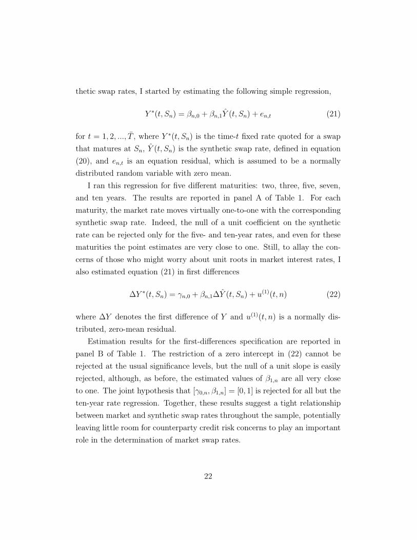
thetic swap rates, I started by estimating the following simple regression,

Y ∗(t, Sn) = βn,0 + βn,1Y (t, Sn) + en,t (21)

for t = 1, 2, ..., T , where Y ∗(t, Sn) is the time-t fixed rate quoted for a swap

that matures at Sn, Y (t, Sn) is the synthetic swap rate, defined in equation

(20), and en,t is an equation residual, which is assumed to be a normally

distributed random variable with zero mean.

I ran this regression for five different maturities: two, three, five, seven,

and ten years. The results are reported in panel A of Table 1. For each

maturity, the market rate moves virtually one-to-one with the corresponding

synthetic swap rate. Indeed, the null of a unit coefficient on the synthetic

rate can be rejected only for the five- and ten-year rates, and even for these

maturities the point estimates are very close to one. Still, to allay the con-

cerns of those who might worry about unit roots in market interest rates, I

also estimated equation (21) in first differences

∆Y ∗(t, Sn) = γn,0 + βn,1∆Y (t, Sn) + u(1)(t, n) (22)

where ∆Y denotes the first difference of Y and u(1)(t, n) is a normally dis-

tributed, zero-mean residual.

Estimation results for the first-differences specification are reported in

panel B of Table 1. The restriction of a zero intercept in (22) cannot be

rejected at the usual significance levels, but the null of a unit slope is easily

rejected, although, as before, the estimated values of β1,n are all very close

to one. The joint hypothesis that [γ0,n, β1,n] = [0, 1] is rejected for all but the

ten-year rate regression. Together, these results suggest a tight relationship

between market and synthetic swap rates throughout the sample, potentially

leaving little room for counterparty credit risk concerns to play an important

role in the determination of market swap rates.

22

6.1 Testing for counterparty credit risk effects

The results reported in Table 1 suggest that market swap rates move nearly

one-to-one with synthetic swap rates derived from Ho-Lee convexity-adjusted

futures rates. It is possible, however, that there are other factors that are

systematically behind fluctuations in market swap rates. Table 2 summarizes

the findings of regressions that examine whether changes in a common proxy

for counterparty credit risk are likely to be one of these missing factors. In

particular, I am interested in whether changes in corporate credit risk spreads

have explanatory power for changes in market swap rates over and above

that provided by changes in the synthetic swap rates. I ran the following

regressions for the same maturities listed in Table 2:

∆Y ∗(t, Sn) = γn,0 + βn,1∆Y (t, Sn) + βn,2∆Y C(t) + u(2)(t, n) (23)

where Y C(t) is the spread between yields on BBB- and AAA-rated corporate

bonds with maturities between seven and ten years, and u(2)(t, n) is a nor-

mally distributed residual, assumed to have zero mean. As can be seen in the

table, the estimated values of βn,2 were statistically insignificant for all ma-

turities, implying that changes in this measure of the market’s perception of

counterparty credit risk have generally not been a factor in the determination

of market swap rates. This insignificance result was unchanged when I used

either the spread of BBB-rated corporate bond yields over Treasury yields

or the spread or BBB-rated corporate yields over AA-rated yields, instead of

the BBB/AAA spread used in the regression results reported in Table 2.

I also ran regressions of the spread between market and synthetic swap

rates on the various proxies for counterparty credit risk,

[Y ∗(t, Sn) − Y (t, Sn)] = τn,0 + τn,1Y C(t) + v(1)(t, n) (24)

where v(1)(t, n) is the normally distributed residual, assumed to have zero

23

mean. I found no systematic effects of Y C on [Y − Y ]. The slope coefficient

was often statistically insignificant and its sign varied from maturity to ma-

turity. Moreover, for all maturities, the estimated coefficients were so small

as to be economically insignificant: The absolute value of τn,1 was always

less than 0.04, implying that a 100 basis point change in Y C is typically

associated with no more than a 4 basis point change in [Y ∗(t, Sn)− Y (t, Sn)].

6.2 Swap valuation during the 1998 market crisis

Although the results obtained thus far have generally downplayed the im-

portance of counterparty credit risk in the determination of swap rates, it

may well be that market participants become especially sensitive to such

risk during times of market stress. That would suggest, for instance, that

the tight relationship between market and synthetic swap rates could have

been significantly disrupted during the fall of 1998, when much of the global

financial markets was in disarray following the Russian default and hedge

fund crises. Did movements in market swap rates at that time systemati-

cally diverge from movements in synthetic rates? Would such a divergence,

if any, be related to heightened concerns about counterparty credit risk? To

address the first of these questions I augmented (22) as follows

∆Y ∗(t, Sn) = γn,0 + βn,1∆Y (t, Sn) + βn,3φ(t) + u(3)(t, n) (25)

where u(3)(t, n) is normally distributed with zero mean. φ(t) is a dummy

variable set to one between the weeks of August 21, 1998 and October 16,

1998—roughly the time period that most people associate with the peak of

the 1998 market crisis—and zero elsewhere.10 Thus, (25) allows the equation

10The week of August 21 immediately followed the Russian default and devaluation ofAugust 17 and the week of October 16 followed the initial easing of monetary policy by theU.S. Federal Reserve, which appeared to have had a calming effect on financial markets.I also experimented with different time intervals for the 1998 crisis, and the main resultswere essentially unchanged.

24

to have an intercept of γn,0+βn,3 during the 1998 financial crisis—when φ(t) =

1—and γn,0 during other times—when φ(t) = 0. Intuitively, the equation

allows for the possibility the market swap rates systematically moved away

from their normal relationship with synthetic rates during the 1998 crisis, in

the sense that the average weekly change in Y ∗(.) during the crisis differed

significantly what would be suggested by changes in Y (.) alone.

The estimation results related to (25) are summarized in panel A of Ta-

ble 3. They suggest no statistically significant role for the dummy variable

φ(t) in the equation intercept as the coefficient βn,3 cannot be statistically

distinguished from zero.

To address the issue of whether swap market participants became partic-

ularly sensitive to changes in counterparty credit risk during the 1998 crisis,

I also estimated the following relationship

∆Y ∗(t, Sn) = γn,0+βn,1∆Y (t, Sn)+[βn,2 +βn,4φ(t)]∆Y C(t)+u(4)(t, n) (26)

where u(4)(t, n) is a normally distributed residual, assumed to have zero mean.

Estimation results based on (26) are reported in panel B of Table 3. The

regressions failed to detect a statistically significant effect of the 1998 crisis on

the sensitivity of market swap rates to the counterparty risk proxy for all of

the maturities examined—the estimated value of βn,4 cannot be statistically

distinguished from zero. These conclusions remained unchanged for the other

two credit risk spreads mentioned above.

Regression results based on the spread between market and synthetic

swap rates also failed to uncover a systematic effect of the 1998 crisis on

swap rates. I estimated the following equation for all maturities analyzed in

Table 3, which simultaneously allows for the 1998 crisis to affect both the

intercept and the slope of (24),

[Y ∗(t, Sn) − Y (t, Sn)] = τn,0 + τn,1Y C(t) + φ(t)[τn,2 + τn,3Y C(t)] + v(2)(t, n)

(27)

25

where v(2)(t, n) is a normally distributed residual with zero mean.

With the exception of a very small but statistically significant τn3 coeffi-

cient for the two-year swap rate, I found no significant crisis effect on either

the slope or the intercept of (27). The finding that the 1998 crisis did not

appear to have a noticeable effect on the relationship between market and

synthetic swap rates can also be checked informally by looking at the time

series of regression residuals associated with equations (21) and (22). As

can be seen in Figures 7 and 8, there does not appear to exist a systematic

difference between the 1998 residuals and those of other years.

7 Sensitivity Analysis

The results obtained thus far suggest that concerns about counterparty credit

risk seem to be largely mitigated by institutional details of the swaps mar-

ket, such as the practices of netting and requiring collateral. Moreover, the

findings are consistent with recent theoretical work—e.g. Duffie and Huang

(1996) and Huge and Lando (1999)—and with the conclusions reached by

Litzenberger (1992). Nonetheless, my results are based, in part, on the spe-

cific assumptions underlying the Ho and Lee model, and one might wonder

about the extent to which these assumptions are are valid, and, more im-

portantly, how sensitive the results are to the particular choice of spot rate

model. Although the Ho and Lee framework has the advantage of being

analytically tractable and easy to apply, in addition to providing an exact

fit to the observed yield curve, it has some drawbacks, such as the fact that

it allows for no mean-reversion in the short rate process, the property that

all spot and forward rates have the same volatility, and the possibility of

negative spot rates. As a result, both to check the sensitivity of the results

to other modeling assumptions and to allay the concerns of those who might

be unhappy with the Ho-Lee model for the short-rate process, I ran the same

26

analysis described above for other widely used models.11

7.1 The Hull and White model

First, I looked at another no-arbitrage model, the one developed by Hull and

White (1990). In its most common form, the Hull-White model assumes that

the risk-neutral process for short rate is given by

dr(t) = [θ(t) − ar(t)]dt + σdX(t) (28)

where X(t) is a standard Brownian motion, θ(t) is a deterministic function

that, as in the Ho and Lee model, allows the model to be calibrated to exactly

fit the observed yield curve, and a and σ are positive constants that need

to be inferred from observable data such as market prices of swaptions of

various maturities.12

As with the the Ho-Lee framework, I calibrated the model to observed

swaptions prices so that, for each time t, a and σ are chosen in order to

minimize the difference between actual and model-implied prices. I then sub-

jected the synthetic swap rates implied by the Hull-White model to the same

battery of tests reported above for the Ho-Lee framework. Results obtained

with the Hull-White model led to virtually the same conclusions reported

above, suggesting that my findings are not peculiar to the assumptions made

by Ho and Lee.

7.2 Estimated Vasicek-type models

I also tested the sensitivity of my results to three alternative models, which

were formally estimated, rather than calibrated. I used the one-factor model

11In appendix A, I provide formulae for the derivation of the convexity adjustment undereach of the models examined in this paper.

12Note that the Hull-White model allows for mean reversion in the short rate: Thespeed of mean reversion is a, and the mean reversion level is given by θ(t)/a.

27

originally proposed by Vasicek (1977), a two-factor extension of the Vasicek

model analyzed in Bomfim (2002), and the one-factor model developed by

Cox, Ingersoll, and Ross (1985).

As in the Hull-White model, the Vasicek model assumes that the short

rate follows a mean reverting process, but, unlike Hull and White, Vasicek

assumes that the short rate reverts to a time-invariant level, l. Indeed, as

the Vasicek model predates Hull and White’s work, the Hull-White model is

also called an extended Vasicek model.

The one-factor Vasicek model assumes that the short rate r(t) evolves

according to

dr(t) = a[l − r(t)]dt + σdX(t) (29)

where, unlike the models examined thus far, the above equation corresponds

to the evolution of r(t) under the real probability measure.

The following two-factor version postulates a similar real process for the

spot rate, except that the level of mean reversion of the spot rate is itself

also assumed to be stochastic and mean reverting:

dr(t) = a[l(t) − r(t)]dt + σdX(t) (30)

dl(t) = b[l − l(t)]dt + ηdW (t) (31)

where both a and b are assumed to be positive; η is the volatility of l(t); l is

the long-term value of the mean-reversion level, and W (t) is assumed to be

a second standard Brownian motion uncorrelated with X(t).13

I estimated the parameters in both the (29) and (30-31) models using a

Kalman-filter-based maximum likelihood procedure.14 The basic conclusions

of the regression analysis comparing actual swap rates to synthetic generated

by the Vasicek-type models confirmed the results obtained with the Ho-Lee

13The assumption of zero correlation allows me to uniquely interpret l(t) and a as thelevel and speed of mean reversion of r(t), respectively (Babbs and Nowman, 1999).

14Bomfim (2002) provides details of the estimation procedure.

28

and Hull-White. Although the estimated one-factor Vasicek model had a

tendency to underestimate the convexity adjustment relative to the other

models, the central result that the futures-implied swap rate and the market

swap rate tend to move one-to-one even during the market stress of 1998 was

still valid.

7.3 The Cox, Ingersoll, and Ross Model

All spot rate models examined so far have the general form

dr(t) = µ(r, t)dt + vdX(t) (32)

where the volatility v of the spot rate r(t) is constant. In addition, these

models have the potentially undesirable property of allowing the spot rate to

become negative. To examine whether these common characteristics of the

models explain why they led me to essentially the same conclusions regard-

ing the importance of counterparty credit risk in the determination of swap

rates, I also examined synthetic swap rates derived from the spot rate model

developed by Cox, Ingersoll, and Ross (1985). The CIR model assumes that

the short rate evolves according to the following real process

dr(t) = a[l − r(t)]dt + σ√

r(t)dX(t) (33)

which is defined under the objective probability measure. (It can be shown

that the CIR model rules out negative spot rates.)

Using parameter estimates reported by Gupta and Subrahmanyam (2000),

I generated synthetic swap rates based on the CIR model and compared them

to market swap rates. Given the parameter values used, the synthetic swap

rates implied by the CIR model tended to underestimate the corresponding

actual swap rates. Nonetheless, regarding the role of proxies for counter-

party credit risk in the determination of swap rates, I generally arrived at

29

the same conclusions reached with the other models. In most regressions,

counterparty credit risk proxies and the dummy variable for the 1998 crisis

had statistically insignificant coefficients attached to them, and even in those

cases where the coefficients were significant, they were very small and, most

likely, economically insignificant.

8 Counterparty Risk and Mid-Market Rates

The analysis in this paper is based on mid-market rates—defined as the

average of the bid and offer rates posted by swap dealers—but one might

argue that a shortcoming of such an analysis is that it is based on quotes

that may be indicative of some “generic” credit quality, rather than on rates

at which transactions actually took place. In response to this argument,

I would make two points. First, in addition Litzenberger’s (1992) work,

conversations with dealers themselves suggest that they do not adjust posted

rates according to the creditworthiness of counterparties, relying, instead, on

credit enhancement mechanisms to manage their exposure to counterparty

credit risk. Second, even if the quoted rates were specific to some generic

credit quality, the meaning of “generic” could well vary according to the credit

environment. For instance, what is considered to be an acceptable risk during

“normal” times might be deemed too risky during times of market stress. If

that were the case, one would, again, see quoted swap rates deviate from

synthetic rates according to the credit environment. I found no evidence of

such deviations.

An alternative potential criticism to the analysis would be that adjust-

ments for the credit quality of counterparties are actually made on the bid

and offer rates quoted by dealers, and it may well be that these adjustments

do not show through in the mid-market rates. For instance, suppose height-

ened concerns about counterparty credit risk lead dealers to post lower paying

rates and higher receiving rates. If such adjustments are always symmetric,

30

they would leave mid-market rates unchanged, and a study based on mid-

market rates, like this paper, would incorrectly conclude that swap rates are

insensitive to concerns about counterparty credit risk.

It turns out, however, that scenarios involving symmetric adjustments to

paying and receiving rates in response to concerns about counterparty credit

risk require some fairly strong assumptions, especially if the symmetry of

adjustments is to be maintained on a day-by-day basis. To see this, recall

that what matters to a rational dealer is the likelihood of the joint event of

default by her swap counterparty while her position in the swap is in the

money. Let us assume at first a flat yield curve. Under such a scenario, the

dealer’s position in the swap is just as likely to be in as out of the money

over some given time horizon and, thus, the dealer needs only care about the

credit quality of its counterparty (Sorensen and Bollier, 1994). Given a flat

yield curve, what additional assumption would I need to guarantee symmetric

adjustments to paying and receiving rates in response to a deterioration in

counterparty credit risk? Suppose that the average credit quality of fixed rate

payers worsens more than that of fixed rate receivers. In this case, the dealer

would increase her receiving rate by more than she would decrease her paying

rate, which would lead to a higher mid-market rate. Thus, with a flat yield

curve, and maintaining the assumption that, rather than adjusting collateral

positions or relying on other credit enhancement mechanisms, the dealer

changes her posted swap rates in response to concerns about counterparty

credit risk, the mid-market swap rate will be insensitive to such concerns only

if the credit quality of her fixed rate payers and receivers always changes to

the same degree. Of course a situation that would be consistent with this

result would be one where fixed payers and receivers always have the same

average credit quality. Nonetheless, such a scenario contradicts some well-

known theories on the rationale for swaps, which suggest that highly rated

entities such as AAA-rated firms and government-sponsored enterprises have

a tendency to be fixed rate receivers in swaps, while lower quality firms tend

31

to be fixed rate payers.15 In this case, symmetric adjustments to paying and

receiving rates would essentially require that whenever the quality of lower

credits deteriorates, that of highly rate entities also worsens to the same

degree, an assumption that may not hold in general, especially in a sample

as long as the one examined in this paper.

What if I relax the assumption of a flat yield curve? Consider, for in-

stance, an upward sloping yield curve. Intuitively, that would suggest that

fixed-paying positions in swaps are now more likely to be in the money in the

future and thus the holders of such positions are more likely to be adversely

affected by a default by their floating rate payers (fixed rate receivers)—

(Duffie and Huang, 1996). Other things being equal, dealers would pay a

lower fixed rate to offset their greater expected exposure and, by the same

logic, would be willing to receive a lower fixed rate. Accordingly, as pointed

out by Sorensen and Bollier (1994), in an upward-sloping yield curve environ-

ment, the creditworthiness of fixed rate receivers becomes more important in

the pricing of swaps than that of fixed rate payers. (The reverse would be

true with an inverted yield curve.) As a result, any adjustments that dealers

might make in swap rates in a response to changes in counterparty credit risk

are generally not symmetric and consequently are likely to leave an imprint

on the mid-market swap rates that are examined in this paper. Thus, the

fact that I detected no such effect in the empirical analysis of market and

synthetic rates suggests that dealers by and large do not adjust their posted

rates in response to changes in counterparty credit risk.

9 Summary and Conclusions

I used various spot rate models to price the convexity differential between

futures and forward contracts. Based on the resulting convexity-adjusted

15Hull (2000) discusses these theories.

32

futures rates, as well as the no-arbitrage relationship between par swap rates

and the forward LIBOR curve, I constructed a series of synthetic swap rates

that can be thought as those that would prevail in a market where swap

rates are not adjusted for counterparty credit risk. These synthetic swap

rates can then be used as benchmarks against which actual swap rates—

those quoted by dealers—can be compared: Other things being equal, any

significant differences between actual and synthetic rates would be indicative

of a non-trivial role for counterparty credit risk in the determination of swap

rates. The analysis detailed in this paper failed to detect any such differences.

The empirical results are also noteworthy in that this paper is the first to

explicitly examine the role of counterparty credit risk in swaps during times

of financial market turmoil. I found that the nearly one-to-one relationship

between synthetic and market swap rates remained relatively intact even

during the 1998 market crisis, which roiled financial markets throughout the

world. On the whole, I interpret these findings as confirming empirically the

view expressed by some that the netting and credit enhancement mechanisms

that are prevalent in the swaps market go a long way in the mitigation of

the role of counterparty credit risk in the determination of swap rates.

It should be noted, however, that the finding of no statistically significant

role for counterparty credit risk in the determination of market swap rates

should not be taken to mean that financial market participants and regula-

tors can simply think of swaps as riskless contracts and ignore the potential

for default-related losses in swap books. After all, it is the very existence

of working procedures for mitigating counterparty risk that is presumably

partly responsible for the lack of sensitivity of swap rates to common proxies

for counterparty credit risk. For instance, effective collateralization requires

efficient monitoring of risk exposures and the existence of reliable mechanisms

for transferring collateral among counterparties.

33

Appendix

A Convexity Adjustment in the Various Mod-

els Used in this Paper

All spot rate models examined in this paper are affine models, i.e., the solu-

tion to the bond pricing PDE has the property that zero-coupon bond yields

are linear functions of the stochastic variables assumed to influence bond

prices—r(t) in the case of the one-factor models, and r(t) and l(t) in the

case of the two-factor model. In particular, for the one-factor models,

P (r(t), t, S) = e−A(t,S)−B(t,S)r(t) (34)

where the forms of A(.) and B(.) depend on the specific model being used.

Equation (34) allows one to write the following general formulae for the

simple (discretely compounded) forward rate:16

f(r(t), t, Si−1, Si) = δ−1i

[eA(t,Si)−A(t,Si−1)+[B(t,Si)−B(t,Si−1)]r(t) − 1

](35)

For the corresponding futures rates, one can derive the following general

formula for the models used in this paper:

F (r(t), t, Si−1, Si) =1

δi

[eA(Si−1,Si)Et[e

B(Si−1,Si)r(Si−1)] − 1]

(36)

and, thus, the convexity adjustment can be computed as the difference be-

tween (36) and (35).17

16Note that for the Ho-Lee and Hull-White models, one can bypass the forward rateformula and use market prices in the right-hand-side of (5). This is because these modelsare calibrated to exactly fit the yield curve, which implies that the model-implied forwardrates will exactly match the ones derived from market prices.

17Formulae for the two-factor model are analogously written with the help of matrix

34

The following is a list of the formulae for A(t, S), B(t, S), and Et[eB(Si−1,Si)r(Si−1)]

for every model used in the text.

• Ho-Lee

B(t, S) = S − t (37)

A(t, S) =

∫ S

t

θ(s)[s − S]ds +σ2[S − t]3

6(38)

θ(s) =∂f ∗(t, s)

∂s+ σ2[s − t] (39)

Et[eB(Si−1,Si)r(Si−1)] = eB(Si−1,Si)Et[r(Si−1)]+

12Vt[r(Si−1)]B(Si−1,Si)

2

(40)

Et[r(Si−1)] = f ∗(t, Si−1) +σ2

2(Si−1 − t)2 (41)

Vt[r(Si−1)] = σ2(Si−1 − t) (42)

where f ∗(t, s) denotes the instantaneous time-t forward for lending or

borrowing at time s, for s > t, derived directly from observed market

prices.

• Hull-White

B(t, S) =1 − e−a(S−t)

a(43)

A(t, S) =

∫ S

t

[.5σ2B(s, S)2 − θ(s)B(s, S)]ds (44)

θ(s) = −∂2logP ∗(t, s)∂s2

− a∂P ∗(t, s)

∂s+ Vt[r(s)](45)

Et[eB(Si−1,Si)r(Si−1)] = eB(Si−1,Si)Et[r(Si−1)]+

12Vt[r(Si−1)]B(Si−1,Si)

2

(46)

Et[r(Si−1)] = f ∗(t, Si−1) +σ2

2B(t, Si−1)

2 (47)

Vt[r(Si−1)] =σ2

2a(1 − e−2a(Si−1−t)) (48)

notation.

35

where where P ∗(t, s) denotes observed zero-coupon bond prices.

• One-factor Vasicek

A(t, S) =

∫ S

t

J(s)ds (49)

B(t, S) =1 − e−a(S−t)

a(50)

Et[eB(Si−1,Si)r(Si−1)] = eB(Si−1,Si)Et[r(Si−1)]+

12Vt[r(Si−1)]B(Si−1,Si)2 (51)

Et[r(Si−1)] = e−a(Si−1−t)r(t) + [1 − e−a(Si−1−t)]l (52)

Vt[r(Si−1)] =σ2

2a(1 − e−2a(Si−1−t)) (53)

where J(s) ≡ (al − λrσ)B(t, s) − .5σ2B(t, s)2 and l ≡ l − λσ/a.

• CIR

A(t, S) = −log

(2γe(a+γ+λ)((S−t)/2)

2γ + (a + γ + λ)(eγ(S−t) − 1)

)2al/v2

(54)

B(t, S) =2(eγ(S−t) − 1)

2γ + (a + γ + λ)(eγ(S−t) − 1)(55)

Et[eB(Si−1,Si)r(Si−1)] =

exp(

B(Si−1,Si)exp(−(a+λ)(Si−1−t))r(t)1−B(Si−1,Si)(v2/2)C(Si−1)

)[1 − B(Si−1, Si)(v2/2)C(Si−1)]2al/v2 (56)

C(Si−1) =1

a + λ(1 − e−(a+λ)(Si−1−t)) (57)

where γ ≡ √(a + λ)2 + 2v2.

• Two-factor Vasicek18

A(t, S) =

∫ S

t

J(s)ds (58)

B(t, S) = (1 − e−a(S−t))/a (59)

18For a = b, C(t, S) becomes (1 − e−a(S−t))/a − (S − t)e−a(S−t).

36

C(t, S) =1

b+

e−a(S−t)

a − b− a

e−b(S−t)

b(a − b)(60)

Et[eAQ(Si−1,Si)Q(Si−1)] = eAQ(Si−1,Si)Et[Q(Si−1)]+ 1

2Vt[Q(Si−1)]AQ(Si−1,Si)2(61)

Et[Q(Si−1)] = e−Ξ(s−t)Q(t) + (I − e−Ξ(s−t))Θ (62)

Vt[Q(Si−1)] =

∫ Si−1

t

e−Ξ(Si−1−u)ΣΣ′e−Ξ′(Si−1−u)du (63)

where J(s) ≡ (al−λrσ)B(t, s)−λlηC(t, s)− .5(σ2B(t, s)2+η2C(t, s)2).

Q(t) ≡ [r(t), x(t)]′; x(t) ≡ l(t) − l, Ξ ≡[

a −a

0 b

], Θ ≡ [l, 0]′, Σ ≡[

σ 0

0 η

], I is a 2x2 identity matrix, AQ(.) ≡ [B(.), C(.)], and Θ ≡

Θ − Ξ−1[λrσ, λlη]′.

37

References

Babbs, S. and B. Nowman, “Kalman Filtering of Generalized Vasicek

Term Structure Models,” Journal of Financial and Quantitative Analy-

sis, 1999, 34, 115–30.

Bank for International Settlements, “The global OTC derivatives mar-

ket at end-December 2001,” 2002. Press Release, May 15.

Belton, T., “Credit Risk in Interest Rate Swaps,” 1987. Working Paper,

Federal Reserve Board.

Bomfim, A., “Monetary Policy and The Yield Curve,” 2002. Working

Paper, Federal Reserve Board.

Burghardt, G., T. Belton, M. Lane, G. Luce, and R. McVey, Eu-

rodollar Futures and Options: Controlling Money Market Risk, Chicago,

IL: Probus, 1991.

Cooper, I. and A. Mello, “The Default Risk on Swaps,” The Journal of

Finance, 1991, 46, 597–620.

Cox, J., J. Ingersoll, and S. Ross, “The Relation Between Forward Prices

and Futures Prices,” Journal of Financial Economics, 1981, 9, 321–46.

, , and , “A Theory of the Terms Structure of Interest Rates,”

Econometrica, 1985, 53, 385–408.

Duffie, D. and K. Singleton, “An Econometric Model of the Term Struc-

ture of Interest Rate Swap Spreads,” The Journal of Finance, 1997, 52,

1287–1321.

and M. Huang, “Swap Rates and Credit Quality,” The Journal of

Finance, 1996, 51, 921–49.

38

Grinblatt, M., “An Analytical Solution for Interest Rate Swap Spreads,”

International Finance Review, 2001.

and N. Jegadeesh, “Relative Pricing of Eurodollar Futures and For-

ward Contracts,” Journal of Finance, 1996, 51, 1499–1522.

Gupta, A. and M. Subrahmanyam, “An Empirical Examination of the

Convexity Bias in the Pricing of Interest Rate Swaps,” Journal of Fi-

nancial Economics, 2000, 55, 239–79.

He, H., “Modeling Term Structures of Swap Spreads,” 2000. Working Paper,

Yale University.

Ho, T. and S. Lee, “Term Structure Movements and Pricing Interest Rate

Contingent Claims,” Journal of Finance, 1986, 41, 1011–29.

Huge, B. and D. Lando, “Swap Pricing with Two-Sided Default Risk in

a Rating-Based Model,” European Finance Review, 1999, 3, 239–68.

Hull, J., Options, Futures, and Other Derivatives, Prentice Hall Interna-

tional Inc., 2000.

and A. White, “Pricing Interest Rate Derivative Securities,” Review

of Financial Studies, 1990, 3, 573–92.

Kamara, A., “Liquidity, Taxes, and Short-Term Treasury Yields,” Journal

of Financial and Quantitative Analysis, 1994, 29, 403–17.

Litzenberger, R., “Swaps: Plain and Fanciful,” The Journal of Finance,

1992, 42, 831–50.

Liu, J., F. Longstaff, and R. Mandell, “The Market Price of Credit Risk:

An Empirical Analysis of Interest Rate Swap Spreads,” 2002. NBER

Working Paper #8990.

39

Minton, B., “An Empirical Examination of Basic Valuation Models for

Plain Vanilla U.S. Interest Rate Swaps,” Journal of Financial Eco-

nomics, 1997, 44, 251–77.

Muelbroek, L., “A Comparison of Forward and Futures Prices of an Interest

Rate-Sensitive Financial Asset,” Journal of Finance, 1992, 47, 381–96.

Newey, W. and K. West, “A Simple Positive Semi-Definite, Heteroskedas-

ticity and Autocorrelation Consistent Covariance Matrix,” Economet-

rica, 1987, 55, 703–8.

Sorensen, E. and T. Bollier, “Pricing Swap Default Risk,” Financial

Analysts Journal, May-June 1994, pp. 23–33.

Sun, T., S. Sundaresan, and C. Wang, “Interest Rate Swaps: An Em-

pirical Investigation,” Journal of Financial Economics, 1993, 36, 77–99.

Sundaresan, S., “Valuation of Swaps,” in S. Khoury, ed., Recent Develop-

ments in International Banking and Finance, Vol. 5, New York: Elsevier

Science Publishers, 1991.

Vasicek, O., “An Equilibrium Characterization of the Term Structure,”

Journal of Financial Economics, 1977, 5, 177–88.

40

Table 1 —Market and Synthetic Swap Ratesa

Y ∗(t, Sn) = βn,0 + βn,1Y (t, Sn) + en,t

∆Y ∗(t, Sn) = γn,0 + βn,1∆Y (t, Sn) + u(t, n)

two years three years five years seven years ten years

A. Levels

constant 0.0275 0.0123 0.0662 0.0133 -0.0743(0.012) (0.013) (0.009) (0.011) (0.020)

synthetic rate 1.0000 1.0006 0.9927 0.9998 1.0194(0.002) (0.002) (0.001) (0.002) (0.003)

R2 0.9987 0.9989 0.9992 0.9989 0.9968Durbin-Watson 0.8123 1.0551 0.9491 0.959 0.437P{H0 : βn,1 = 1}b 0.99 0.70 0.00 0.90 0.00P{H0 : [βn,0, βn,1] = [0, 1]} 0.00 0.00 0.00 0.00 0.00

B. First Differences

constant -0.0001 -0.0000 -0.0000 -0.0000 -0.0001(0.001) (0.001) (0.001) (0.001) (0.001)

synthetic rate 0.9255 0.9458 0.9686 0.9674 0.9849(0.028) (0.020) (0.014) (0.015) (0.016)

R2 0.9228 0.94351 0.9594 0.9523 0.9408Durbin-Watson 2.9341 2.9905 2.9610 2.8616 2.7417P{H0 : βn,1 = 1} 0.00 0.00 0.00 0.00 0.21P{H0 : [γn,0, βn,1] = [0, 1]} 0.00 0.00 0.00 0.00 0.37

aEstimation period: January 7, 1994 to March 22, 2002 (428 weekly observations).Heteroskedasticity- and autocorrelation-consistent standard errors shown in parenthesis (Neweyand West, 1987).

bP{.} denote P-values associated with null hypothesis shown in brackets.

41

Table 2 —Testing for Counterparty Credit Riska

∆Y ∗(t, Sn) = γn,0 + βn,1∆Y (t, Sn) + βn,2∆Y C(t) + v(t, n)

two years three years five years seven years ten years

constant -0.0001 -0.0001 -0.0001 -0.0001 -0.0000(0.001) (0.001) (0.001) (0.001) (0.001)

synthetic rate 0.9252 0.9472 0.9705 0.9690 0.9856(0.028) (0.020) (0.014) (0.015) (0.015)

BBB/AAA spread -0.0040 0.0226 0.0331 0.0264 0.0121(0.039) (0.033) (0.028) (0.028) (0.028)

R2 0.9226 0.9434 0.9594 0.9522 0.9407Durbin-Watson 2.9339 2.9914 2.9613 2.8584 2.7403

aEstimation period: January 7, 1994 to March 22, 2002 (428 weekly observations).Heteroskedasticity- and autocorrelation-consistent standard errors shown in parenthesis (Neweyand West, 1987).

42

Table 3 —Swap Valuation during the 1998 Market Crisisa

two years three years five years seven years ten years

A. ∆Y ∗(t, Sn) = γn,0 + βn,1∆Y (t, Sn) + βn,2φ(t) + v(t, n)

constant -0.0001 -0.0001 -0.0001 -0.0001 0.0001(0.001) (0.001) (0.001) (0.001) (0.001)

synthetic rate 0.9249 0.9456 0.9685 0.9670 0.9845(0.028) (0.021) (0.014) (0.015) (0.015)

dummy (φ(t)) -0.0031 -0.0013 -0.0003 -0.0037 -0.0049(0.009) (0.010) (0.007) (0.007) (0.007)

R2 0.9226 0.9434 0.9593 0.9522 0.9407Durbin-Watson 2.9334 2.9905 2.9610 2.8628 2.7421

B. ∆Y ∗(t, Sn) = γn,0 + βn,1∆Y (t, Sn) + [βn,2 + βn,3φ(t)]∆Y C(t) + v(t, n)

constant -0.0001 -0.0001 -0.0002 -0.0001 -0.0001(0.001) (0.001) (0.001) (0.001) (0.010)

synthetic rate 0.9252 0.9471 0.9703 0.9689 0.9856(0.028) (0.020) (0.014) (0.015) (0.015)

BBB/AAA spread -0.0072 0.0129 0.0186 0.0220 0.0093(0.050) (0.039) (0.034) (0.035) (0.035)

dummy (φ(t)∆Y C(t)) 0.0089 0.0279 0.0414 0.0127 0.0080(0.081) (0.074) (0.062) (0.060) (0.059)

R2 0.9224 0.9433 0.9593 0.9521 0.9406Durbin-Watson 2.9345 2.9940 2.9661 2.8598 2.7409

aEstimation period: January 7, 1994 to March 22, 2002 (428 weekly observations).Heteroskedasticity- and autocorrelation-consistent standard errors shown in parenthesis (Neweyand West, 1987).

43

94 95 96 97 98 99 00 01 02 030

20

40

60

80

100

120

140

Ba

sis

Po

ints

2−year5−year10−year

Figure 1Historical Swap Spreads

* The figure shows spreads of two-, five-, and ten-year swap rates over yields on U.S. Treasury debt

securities of comparable maturities.

44

2 3 4 5 6 7 8 9 105.8

5.9

6

6.1

6.2

6.3

6.4

6.5

6.6

6.7

6.8

maturity (years)

pe

rce

nt

ActualImplied by futures

Figure 2Average swap curve (Jan 1994 − Mar 2002)

* For each maturity listed in the horizontal axis, the figure shows the average actual swap rate and the

average futures-implied swap rate over the entire January 1994–March 2002 sample. The underlying data

are composed of weekly observations.

45

93 94 95 96 97 98 99 00 01 02 0350

100

150

200six−month/five−year swaption

93 94 95 96 97 98 99 00 01 02 03100

150

200

250one−year/five−year swaption

93 94 95 96 97 98 99 00 01 02 03150

200

250

300two−year/five−year swaption

93 94 95 96 97 98 99 00 01 02 03200

250

300

350

400five−year/five−year swaption

93 94 95 96 97 98 99 00 01 02 030.6

0.8

1

1.2

1.4Memo: Short Rate Volatility (percentage points)

Figure 3

Actual and Theoretical Swaption Prices*

*Swaption prices (the solid lines) are in US dollars and correspond to options to enter into a five−year swap with a notional principal of $10,000. Theoretical prices (the dashed lines) are based on the Ho−Lee model. The lower panel shows the values of the short rate volatility paramenter (σ) that allowed the model to best fit the quoted prices.

46

2 3 4 5 6 7 8 9 105.8

5.9

6

6.1

6.2

6.3

6.4

6.5

6.6

6.7

6.8

maturity (years)

pe

rce

nt

ActualImplied by futuresSynthetic

Figure 4Average swap curve (Jan 1994 − Mar 2002)

* For each maturity listed in the horizontal axis, the figure shows the average actual swap rate, the

average futures-implied swap rate, and the average synthetic swap rate over the entire January 1994–March

2002 sample. (The solid and dashed curves are the same ones shown in Figure 2.) The underlying data are

composed of weekly observations.

47

2 3 4 5 6 7 8 9 104

4.5

5

5.5

6

6.5

maturity (years)

pe

rce

nt

ActualImplied by futuresSynthetic

Figure 5Swap curves (week ending March 22, 2002)

* The figure shows the actual swap curve, the futures-implied swap curve, and the synthetic swap curve

on the week ending March 22, 2002. (Figures 2 and 4 showed average rates over the 1994/2002 sample,

which included this particular week.)

48

9495

9697

9899

0001

0203 2

4

6

8

10

−50

0

50

maturity (years)

Figure 6: Spread between Actual and Synthetic Swap Rates

Time

ba

sis

po

ints

* The figure shows differences (in basis points) between actual and synthetic swap rates over time and

across various maturities.

49

95 96 97 98 99 00 01 02

−20

−10

0

10

20

two−year rate

95 96 97 98 99 00 01 02

−20

−10

0

10

20

three−year rate

95 96 97 98 99 00 01 02

−20

−10

0

10

20

basis

poi

nts

five−year rate

95 96 97 98 99 00 01 02

−20

−10

0

10

20

seven−year rate

95 96 97 98 99 00 01 02

−20

−10

0

10

20

ten−year rate

Figure 7

Residuals of Levels Regressions

* The figure shows the residuals from regressing market swap rates with the maturity indicated in each

panel on a constant and on the corresponding synthetic swap rate.

50

95 96 97 98 99 00 01 02

−20

−10

0

10

20

two−year rate

95 96 97 98 99 00 01 02

−20

−10

0

10

20

three−year rate

95 96 97 98 99 00 01 02

−20

−10

0

10

20

basis

poi

nts

five−year rate

95 96 97 98 99 00 01 02

−20

−10

0

10

20

seven−year rate

95 96 97 98 99 00 01 02

−20

−10

0

10

20

ten−year rate

Figure 8

Residuals of First−Differences Regressions

* The figure shows the residuals from regressing changes in market swap rates with the maturity

indicated in each panel on a constant and on changes in the corresponding synthetic swap rate.

51