MS Thesis

Reykjavík Energy Graduate School of Sustainable Systems

Costs, Profitability and Potential Gains of the CarbFix Program

Elisabet Vilborg Ragnheidardottir

Business Department University of Iceland

Advisors: Helga Kristjansdottir

William Harvey

Holmfridur Sigurdardottir

January, 2010

iii

ABSTRACT

This paper aims to review the costs associated with the CarbFix injection program and

determine its possible revenues. The CarbFix costs are reviewed both in its current pilot

project state, as well as two larger scenarios involving the Hellisheidi geothermal power

plant in southwest Iceland and a pulverized coal plant. The Simple Multi-attribute

Technique (SMART) combined with a PESTLE analysis provides a detailed portfolio of

positive markets that CarbFix could enter with its knowledge to provide a service. While

costs of storage of CO2 in other types of reservoirs have been widely studied, there are

limited data on storage through mineralization. The largest cost contributors for both the

CarbFix pilot program and the Hellisheidi plant are the capital and monitoring costs, but

water and electricity costs become more predominant in the pulverized coal case. This

paper, specifically through its cost analysis, adds much needed information on the

economics of this emerging form of CCS. The cost analysis shows that the cost per tonne

of CO2 emitted would need to be 77!/tCO2 for the Hellisheidi scenario to be profitable

while the pulverized coal scenario would be profitable at 50!/tCO2 emitted. The market

analysis shows that the most efficient markets, in terms of low barriers to entry and

adequate purchasing power, are Russia, the United States, Canada, Italy and Germany.

KEYWORDS: carbon capture and storage; mineral carbonation; CarbFix; carbon dioxide;

Hellisheidi; Iceland

iv

TABLE OF CONTENTS

Abstract ........................................................................................................................... iii

I. Introduction.................................................................................................................11

II. Literature Review........................................................................................................15

II.1 Geological Storage ...............................................................................................15

II.2 Mineral Carbonation.............................................................................................18

II.3 Carbon Capture & Storage....................................................................................20

II.4 Associated Risks...................................................................................................22

II.5 Liability................................................................................................................24

II.5.1 Short-term versus Long-term.......................................................................24

II.5.2 Insurance .....................................................................................................25

II.5.3 Multiparty Liability .....................................................................................27

II.6 Regulations...........................................................................................................28

II.6.1 Classification of CO2 ...................................................................................28

II.6.2 Pore Space Ownership.................................................................................29

II.6.3 Licensing & Permits ....................................................................................29

II.7 Incentives .............................................................................................................30

II.8 Economics............................................................................................................31

II.8.1 Capture........................................................................................................33

II.8.2 Transport .....................................................................................................38

II.8.3 Storage ........................................................................................................40

v

II.8.4 Monitoring ..................................................................................................42

II.8.5 Total CCS Costs ..........................................................................................43

II.9 PESTLE Analysis.................................................................................................44

II.10 Simple Multi-Attribute Rating Technique .....................................................45

III. Techno-Economic Scenarios.................................................................................47

III.1 CarbFix – Present Status & Methodology .............................................................47

III.1.1 H2S Abatement System .........................................................................48

III.1.2 Basalt ....................................................................................................49

III.1.3 CarbFix methodology............................................................................50

III.2 CarbFix Pilot Program..........................................................................................52

III.2.1 Data ......................................................................................................52

III.2.2 Cost Analysis ........................................................................................55

III.2.3 Profitability Assessment........................................................................59

III.3 Hellisheidi full-scale scenario ...............................................................................63

III.3.1 Data ......................................................................................................63

III.3.2 Injection well calculations.....................................................................64

III.3.3 Cost analysis .........................................................................................65

III.3.4 Profitability assessment .........................................................................69

III.4 CarbFix applied to a pulverized coal plant ............................................................72

III.4.1 Coal ......................................................................................................72

III.4.2 Existing plant and data ..........................................................................74

III.4.3 Cost analysis .........................................................................................75

III.4.4 Profitability assessment .........................................................................77

IV. Market Analysis ...................................................................................................81

IV.1.1 Methodology.........................................................................................81

IV.1.2 Attribute descriptions ............................................................................86

vi

IV.1.3 Purchasing power parity........................................................................91

IV.2 Data..................................................................................................................92

IV.3 Efficiency frontier ............................................................................................92

IV.4 Sensitivity analysis ...........................................................................................93

V. Conclusions.................................................................................................................97

References .....................................................................................................................101

vii

LIST OF FIGURES

Figure 1: CO2 captured vs. CO2 avoided...........................................................................32

Figure 2: Separation process of CO2 through chemical solvents. ......................................34

Figure 3: Costs for CO2 transport as a function of CO2 mass flow rate. ............................39

Figure 4: Levelized costs for CO2 transport as a function of CO2 mass flow rate. .............40

Figure 5: Well drilling cost as a function of depth. ...........................................................42

Figure 6: N-S geological cross section of the injection site, including injection well (HN-2)

and monitoring wells. ...............................................................................................51

Figure 7: Percentage breakdown of total capital costs for pilot program ...........................56

Figure 8: Percentage breakdown of total annual costs for pilot program. ..........................57

Figure 9: Sensitivity Analysis of annual cost factors, pilot program..................................58

Figure 10: Sensitivity Analysis of annualized capital costs, pilot program. .......................58

Figure 11: Accumulated Net Present Value of the CarbFix Pilot Program at 900!/tCO2. ..61

Figure 12: Debt Cover Ratios of the CarbFix Pilot Program at 900!/tCO2........................62

Figure 13: Accumulated Net Present Value of the CarbFix Pilot Program at 1.200!/tCO2.

.................................................................................................................................62

Figure 14: Changes in costs from pilot program to full-scale program. .............................67

Figure 15: Sensitivity Analysis of annual cost factors, full-scale program.........................67

Figure 16: Sensitivity Analysis of annualized capital costs, full-scale program.................68

Figure 17: Sensitivity Analysis of annualized capital costs, full-scale program with 10

injection wells. .........................................................................................................69

Figure 18: Accumulated Net Present Value of the Hellisheidi Full-Scale Program at

50!/tCO2. .................................................................................................................70

Figure 19: Accumulated Net Present Value of the Hellisheidi Full-Scale Program at

77!/tCO2. .................................................................................................................71

viii

Figure 20: Debt Cover Ratios of the Hellisheidi Full-Scale Program at 77!/tCO2. ............71

Figure 21: Sensitivity Analysis of annual cost factors, PC plant with 17 wells..................77

Figure 22: Internal Rate of Return on total cash flow and net cash flow for the Pulverized

Coal case with CarbFix at 13!/tCO2. ........................................................................78

Figure 23: Accumulated Net Present Value of the Pulverized Coal program with CarbFix

at 50!/tCO2. .............................................................................................................79

Figure 24: Debt Cover Ratios of the pulverized coal scenario at 50!/tCO2........................79

Figure 25: Value tree of PESTLE attributes by their category...........................................82

Figure 26: World map indicating countries that were used in the market analysis. ............92

Figure 27: Market analysis efficiency frontier. .................................................................93

Figure 28: Sensitivity analysis of the top three ranked weights in each category, Threats

and Opportunities. ....................................................................................................94

Figure 29: Natural gas production in tera joules per year by country.................................95

Figure 30: Changes in the weight of natural gas; lower performing countries. ..................95

Figure 31: Changes in the weight of natural gas: higher performing countries. .................96

ix

LIST OF TABLES

Table 1: Review of the costs for CCS according to the literature. .....................................43

Table 2: Most likely cost and applied cost of transport and injection of CO2 sequestration

.................................................................................................................................53

Table 3: Cost summary for carbon mineralization. ...........................................................55

Table 4: Economic parameters used for profitability assessment of the CarbFix pilot

program....................................................................................................................60

Table 5: Resulting profitability ratios from varying prices of !/tCO2, pilot program. ........63

Table 6: Cost increase for full-scale Hellisheidi program..................................................66

Table 7: Resulting profitability ratios from varying prices of !/tCO2, Hellisheidi full-scale

scenario....................................................................................................................72

Table 8: Characteristics overview of a 308 MWe reference pulverized coal plant and PC

plant with capture. ....................................................................................................75

Table 9: Cost increase for PC plant using CarbFix............................................................76

Table 10: Resulting profitability ratios from varying prices of !/tCO2, PC plant with

CarbFix. ...................................................................................................................80

Table 11: List of attributes, their unit, and the source and base year for the SMART

analysis. ...................................................................................................................83

Table 12: Attribute ranks, swing weights and normalized weights. ...................................85

11

I. INTRODUCTION

The world is currently in a battle against increasing levels of carbon dioxide (CO2) in the

atmosphere and its negative effect on the environment. As economies and nations grow,

driven by continuous population increase, the emissions of those nations and their

industries add to global CO2 emissions. While energy efficiency and fuel choice for

electrical production remain driving forces in decreasing greenhouse gases, another path is

currently being pursued that not only could decrease emissions but also participate in

macroeconomic trading markets. Carbon, capture and storage (CCS) is a method by which

CO2 is captured as a clean stream and re-injected into various geological formations for the

purpose of long-term storage. Mineral carbonation is an option by which this re-injection

and storage of CO2 could take place. By fixing CO2 as a stable mineral the natural

weathering processes are replicated and nature is imitated, specifically in the CarbFix case

by using basalt to produce carbonates. CarbFix aims to test in-situ mineral sequestration of

CO2 by utilizing geothermal gases produced from the Hellisheidi geothermal power plant

located in southwest Iceland.

The questions that this thesis will specifically answer are the following:

1. What is the cost of storing one tonne of CO2 (tCO2) in the CarbFix pilot program?

2. What is the cost of storing one tCO2 using the CarbFix method for larger flow rates

of CO2?

3. What are the main cost drivers of the CarbFix method of CCS?

4. What is the possible revenue that may be achieved in relation to the determined

costs and differing prices of CO2 available on the market?

5. What are the positive markets with low barriers to entry that CarbFix should focus

on in the future?

Chapter 2 will review the literature of carbon capture and storage. The review provides an

oversight as to the total costs that are known today through both studies and research pilot

programs similar to the CarbFix program. The literature however distinctly shows that

while the costs for storage of CO2 in alternative sites, such as aquifers and oil fields, are

12

well known, cost information associated to mineral carbonation is limited. This paper adds

to the large portfolio of information on CCS as a process by identifying cost drivers of

mineral carbonation. The resulting information from this thesis will help to focus future

work, both engineering and geological, as to where sensitive points of the project lie

economically.

The third chapter models both technological and economical scenarios. The goals of the

chapter are to analyze the costs for three separate scenarios that differ in CO2 flow rate.

The first scenario considers the current CarbFix pilot program while the other two

scenarios are scaled up models, which assess the Hellisheidi geothermal power plant and a

pulverized coal plant. The capital and annual costs, such as water and energy, are scaled

from the pilot program as well as known geophysical requirements in order to achieve

correct geochemical reactions. A cost analysis is done by assessing both capital costs and

variable costs associated with water and energy, and determine an estimated cost per tCO2

stored. By analyzing the changes in the costs according to the differing flow rates the

sensitive cost factors are identified in order to better focus future work on where cost

reductions are needed. Specifically the costs associated with water and energy

requirements are modelled, reviewed and analyzed in order to better understand the effect

on the total costs per tonne.

As Chapter 3 provides a list of factors that dominate the resulting cost per tCO2 it is

important to know exactly how sensitive the cost is to variations in these factors. A Monte

Carlo simulation shows the sensitivity of the levelized cost to changes in those factors. The

results are important in order to understand the need for accurate cost estimates in the

beginning of the project and also determine in what range the capital costs must lie in order

for the levelized cost to lay within a corresponding range. However, as the flow rate is such

a dominant factor in the cost assessments for the large flow scenario, the pulverized coal

plant is also tested for its sensitivity to changes in water and energy requirements.

Chapter 3 also includes a profitability assessment for each scenario. The purpose is to

accurately identify at what cost per tCO2 the market must provide in order for the

scenarios, at current costs, to realize revenue. Carbon trading on the global market is

increasing due to public and political pressure to reduce greenhouse gases while still

providing a free market solution. Additionally, carbon taxes on energy related CO2 are not

uncommon in Europe and as governments try to produce additional state income while

reducing carbon dioxide emissions immobile emitters of CO2 must consider compliance

13

options. This paper then provides clues as to at what price the tax would need to be in

order for CarbFix to be an attractive option in lieu of paying the tax. Lastly, international

agreements such as the Kyoto Protocol provide nations with options to achieve emission

targets. In order for CarbFix to present this service as an option, to both nations and

corporations within those nations, the cost must be accurately defined in order to better

develop prices at which the service is offered.

As CarbFix is producing an industrial method for CO2 storage it is important to recognize

its future possibilities as revenue for Orkuveita Reykjavikur (Reykjavik Energy). This

possibility lies not only within the borders of Iceland but also on a global level and is the

main focus of Chapter 4. More international pressure on countries to reduce greenhouse

gas emissions is creating a more open market for companies that possess tools to realize

this goal. However, marketing a product in any given country can be an expensive and

lengthy process. Being aware of the proper countries to perform this marketing is

important and executing this action in the most efficient way a priority. The market

analysis in this chapter identifies the key factors that create a positive market for CarbFix

both through identifying opportunities and threats. The methodology includes identifying

attributes using the PESTLE analysis and then rating the attributes using the Simple Multi-

Attribute Rating Technique. The analysis also takes into account the purchasing power of

the country’s currency in order to identify countries that have a lower purchasing barrier.

The results from the market analysis provide a short list of those countries that are the most

viable markets for CarbFix to enter. Due to the prescriptive nature of the SMART analysis

a sensitivity analysis is also employed in order to better understanding the driving factors

that produce this short list of countries. The analysis only presents results according to the

preferences of the decision maker as elicited through the attributes. By changing the weight

of the top ranking attributes the changes in the top performer countries are shown.

Chapter 5 will bring together the results of each of the chapters in order to provide an

overall conclusion. The technological and economical models show the strong relationship

between the flow rate of CO2 and the resulting cost per tonne. This is due to the linear

relationship between the flow rate and the water requirements. The energy requirements

are also driven by the CO2 flow rate. The costs, while high in the pilot program, become

competitive at large flow rates when compared to the information in the literature review.

The information in Chapter 5 will also provide insight into the role of the number of

required wells. This accentuates the importance of the number of wells being determined

14

both for injection as well as monitoring. The Hellisheidi full-scale scenario is also one with

a dynamic that may change in the near future. The increased electrical production, and as

such annual CO2 emissions, can help to drive down costs in the future at the current costs.

All of these factors combined result in a program that may be highly competitive and a

viable service product in the future. The costs known and used for analysis in this thesis

are still on a preliminary basis as this is a pilot program. Internal learning through doing

may lead CarbFix to be a leader in the carbon mineralization method of carbon capture and

storage.

The market analysis provides a short list based on the attributes utilized in the SMART

analysis as well as the purchasing power of the market. It is important to note that while

some countries do not lie on the efficiency frontier, which produces the short list, they may

be acceptable markets to enter in the future. For example, Malaysia provides an adequate

attribute score and has sufficient power purchasing but does not lie on the efficiency

frontier. It is however the sensitivity of one particular attribute, natural gas, that provides

the most interesting information. While it was not listed as being the highest weighted

attribute it is found to be the most prominent attribute in terms of sensitivity in the

resulting markets. Natural gas production requires CO2 to be removed in order for the

natural gas to reach its required quality for sale. Tax associated to CO2 emissions from

natural gas has already motivated one company to turn to carbon storage as an alternative

option to the tax. Being aware of this key aspect can help CarbFix in the future to remain a

living organism capable of adapting as other countries possibly adopt this tax.

15

II. LITERATURE REVIEW

II.1 Geological Storage

Geological sequestration of carbon dioxide is in itself not a new idea towards the lowering

of atmospheric emissions. In fact, natural underground CO2 fields are present around the

world and have existed for geological timescales1 (Holloway, 2005). To date research has

mainly focused on depleted oil and gas fields, non-economic coal beds and saline aquifers

(Oelkers & Cole, 2008; Benson & Cole, 2008). The literature review and this Chapter

discuss the injection of CO2 into these types of formations where pressures and

temperatures are above the critical point, or 7,38 Mega Pascal (MPa) and 31,6°C2. These

formations are at depths of more than 1.000 m (McGrail et al., 2006).

Gas and oil fields are natural pools of trapped gases and fluids. They are covered by a cap

rock, which has trapped the oil and gas before exploitation by man. Once these fields are

depleted they can be used to re-inject CO2 and store it stably. The setup could be minimal

as most of the existing infrastructure, such as wells and geophysical data, can be re-used

and this would help minimize capital costs; however it may be necessary to drill new

injection wells instead of using the existing ones if the quality of the well has degraded

(IEA, 2004). Also, previous extraction of oil and gas must not damage or fracture the cap

rock (Holloway, 2005). Because there is usually no water present in gas fields the volume

of CO2 possible to store could be approximately equal to the volume of gas that was

present beforehand (Holloway, 2005).

Coal beds have fractures called cleats. Pores present in the cleat contain gas known as coal

bed methane (CBM). The methane is absorbed into the pores but is dependent on

temperature and pressure and can, depending on changes in these two factors, be desorbed

1 Periods of time as defined by significant historical and geological events such as mass extinction. 2 When CO2 is injected into reservoirs with a temperature above 31,1°C and a pressure above 7.39 MPa it is said to be at its supercritical state in where it has the properties between that of being a gas and a liquid.

16

(Davidson, 1995 as cited by Holloway, 2005). Once the CO2 is pumped into this type of

reservoir it can absorb onto the coal and can be held in place, dependent on temperature

and pressure (Holloway, 2005). The methane recovered when CBM is released can

additionally have economic value, which can then offset the sequestration costs. This was

first tested on a large scale at the San Juan Basin in New Mexico. In 1995 CO2 was

injected through multiple wells and led to an increase in methane recovery from 77% to

95%. The total amount of CO2 injected over the following six years was 370 thousand

tonnes (Mazzotti, Pini & Storti, 2009).

Statoil in Norway is performing an industrial-scale example of the geological storage of

CO2 in a saline aquifer. In order to produce saleable natural gas according to consumable

specifications the CO2 is stripped (Alphen, Ruijven, Kasa, Hekkert & Turkenburg, 2009).

The CO2 is then re-injected into the offshore Sleipner West gas field and has been

operating since 1996 at a rate of 1 mega tonne (Mt) CO2 per year (Holloway, 2005; Torp &

Gale, 2004). The area in which Statoil is re-injecting is the Utsira formation, which is an

offshore sand bed 800-1.000 meters below the sea bottom and 150-200 m thick (Holloway,

2005; Torp & Gale, 2004). The purpose of this sequestration scheme was mainly due to

financial burdens that would have otherwise been incurred due to a carbon tax, !40 per

emitted tonne3, for offshore petroleum activities (Karstad, 1992 as cited by Alphen et al.,

2009). The extra costs to Statoil from this operation are $15 per tCO2 avoided4 (Herzog,

1999).

The sequestration of supercritical CO2 in basalt, depleted oil or gas reservoirs, coal beds

and aquifers all require an impermeable cap rock. This is due to the nature of CO2 at

various conditions but specifically its tendency to be more buoyant than in-situ fluids

(Benson & Cole, 2008; Oelkers & Cole, 2008). When the CO2 pervades the reservoir rock

the fluid that filled the rock’s pores is pushed out and the CO2 fills the space. Any barriers

to flow through the reservoir of the in-situ5 fluids can limit the amount of CO2 possible to

inject because of the pressure increases (Holloway, 2005). The migration behaviour of CO2

is dependent on the pore fluid’s properties; that is whether the CO2 will be miscible or

immiscible. Miscible means that the CO2 can mix completely with the pore fluid to form a

3 The tax was introduced in 1991. 4 In 1999 USD. 5 In-situ is a Latin phrase meaning literally “in its original place”.

17

single phase, whereas immiscible means the two phases remain separate (Benson & Cole,

2008).

The cap rock plays an important role, as the re-injection reservoir does not require a dome

shaped structure such as oil or gas fields. The reservoir can be flat as long as it is large

enough that the CO2 will simply rise until it reaches the cap rock. When the structure has

reached its full storage capacity the CO2 could spill out and follow migration paths of

interlocked pores and begin to fill any connecting formations (Holloway, 2005).

The options discussed for geological sequestration have incredible potential for storage as

they are estimated to have the capacity of up to 3,3 teratonnes (Tt) of CO2 in oil and gas

reservoirs, 36,7 Tt in saline aquifers and 734 gigatonnes (Gt) in unmineable coal beds6

(IPCC, 2005). As a comparison the annual CO2 emissions from fuel combustion in the

world are approximately 29 Gt (IEA Statistics, 2009). There are large uncertainties in

regards to the actual capabilities of storage. The storage potential will vary by region and

so a case-by-case analysis is always important and no real standardization analysis method

is available (IPCC, 2005).

Enhanced oil recovery (EOR) and enhanced gas recovery (EGR) are techniques used

currently in various locations and represents a more economical approach to CO2 re-

injection. EOR is the process by which additional oil is recovered through various

processes, one of which is the injection of supercritical CO2. The CO2 displaces residual oil

that was not removed during primary production or secondary recovery (Ravagnani, Ligero

& Suslick, 2009). EGR is a similar process in which CO2 is used to displace residual

natural gas in mature reservoirs (Solomon, Carpenter & Flach, 2008). The additional oil or

gas recoverable can offset the sequestration costs (Holloway, 2005).

EOR increases the recovery of original oil by 50% and EGR a 5 to 15% increase in gas

recovery (IEA, 2004). Even though these two techniques seem to be economical options to

offset CCS costs, they are sensitive to location. In general the farther the distance of the

injection reservoir from the point source of the CO2 emissions, the higher costs are for

transportation (IEA, 2004). However, in EGR and EOR the cost of injecting CO2 is limited

to the increased value in the additionally produced gas or oil, and the cost for

6 Original values were given in amounts of carbon. One tonne of carbon, when combined with oxygen to produce CO2, has a mass of 3,67 tonnes.

18

transportation must not exceed this threshold. The deployment of CCS for the purpose of

EOR or EGR may be one of the key driving factors for the overall deployment of CCS as

an emissions reducer. Economics for EOR and EGR will lead to a market in which the

emitter can sell the CO2 to another entity, for example an oil production company, who is

attempting to increase their oil or gas production. Through increasing attempts by the

emitter to capture CO2 in an economical manner, at the lowest possible cost in order to

achieve the highest net gains, there may be a gain in technological knowledge through

learning by doing.

II.2 Mineral Carbonation

Fixing CO2 as a mineral is referred to as mineral carbonation and results in calcite

(CaCO3), dolomite (CaMg(CO3)2), magnesite (MgCO3), siderite (FeCO3), and magnesium-

iron carbonate solid solutions (Oelkers, Gislason & Matter, 2008), which are stable over

geologic timescales and thus not prone to leakage (Oelkers & Cole, 2008). The process

itself is a naturally occurring one and referred to as silicate weathering. The

Intergovernmental Panel on Climate Change, IPCC, (2005) identified mineral carbonation

as one such method to produce stable elements over long periods with a retention rate7 of

near 100%. The IPCC however mainly addresses mineral carbonation as an ex-situ8

process in which the minerals would need to be mined and transported and after the

carbonation processes has taken place, the resulting carbonate contained in a waste site.

Hepple and Benson (2002) find in their research that an acceptable leakage rate for

geological sequestration was less than 1% per year. Their analysis considers six allowable

emissions levels to reflect the emissions scenarios set out by the IPCC Special Report on

Emissions Scenarios within a 300-year timeframe. It is however noted that mineralization

of CO2 would decrease the migration towards the surface (Hepple & Benson, 2002).

In order to fix the CO2 and produce these stable minerals there is a need for, in addition to

the CO2 itself, divalent cations9 such as Ca2+, Mg2+ and Fe2+(Gislason et al., 2009). The

groundwater present in basaltic rocks in Iceland has been found to be rich in Ca2+ and

7 The retention rate is the percent of CO2 that remains in the injection site and does not leak in the long-term. 8 Ex-situ is the opposite of in-situ and refers to operations “off site”.

19

Mg2+(Arnorsson et al., 2003 as cited by Gislason et al., 2009). When CO2 is exposed to

this groundwater the reaction follows:

(Fe2+, Ca2+, Mg2+) + CO2 + H2O = (Fe,Ca,Mg)CO3 + 2H+ (1)

Oelkers et al. (2008) estimated that each one tonne of carbon to be fixed (approximately

3,67 tCO2) requires 8,8 tonnes of basaltic glass10. The precipitation of carbonates is

dependent on the pH. As the basalt dissolution increases the amount of cations available

increases and thus increases the pH until the precipitation begins (Matter et al., 2008).

Additionally the dissolution rate is increased with a lower silica content of the reactive

rock (Alfredsson, Hardarson, Franzson & Gislason, 2008). Through tracer tests it has been

confirmed that the basaltic bedrock at the Hellisheidi injection site is made up of

homogeneous porous media and thus a network of interconnected pore space for a large

reactive surface area (Khalilabad, Axelsson, Gislason, 2008).

An area being studied that is comparable to the CarbFix project is the Columbia River

Basalts Group (CRBG) in the United States, specifically in the states of Washington,

Oregon and Idaho. Its land coverage is 164.000 km2 and is estimated to have a volume of

174.000 km3. McGrail et al. (2006) state that the storage potential of this area is 100 Gt of

CO2. The area in the CarbFix pilot study is able to accommodate 12 Mt of CO2 (Gislason

et al., 2009)11. In comparison to this volume it takes 2.3 m3 to fix the CO2 produced

annually by one car and the human produced annual emissions from large industries12 is 29

Gt of CO2 (Oelkers & Cole, 2008).

The CRBG is made up of multiple lava flows and shows significant porosity as well as a

cap rock in the form of low-permeable interbedded sediments and impermeable basalt

between interflow zones (McGrail et al., 2006). Samples from the CRBG in the laboratory

have produced carbon mineralization when exposed to water and supercritical CO2.

9 Divalent cations are atoms that are missing electrons when they are compared to their elemental state. 10 This is assuming 100% dissolution of the mineral and glass and that all divalent cations end up in carbonates. 11 This is assuming that there is 10% porosity in the rock and 10% of the pores are filled with calcite. 12 These are emissions primarily from coal, oil, natural gas, and the production of cement. Their emissions constitute, of total CO2 emissions, 36%, 42%, 18% and 4% respectively (Oelkers & Cole, 2008).

20

Another finding from McGrail et al. that may have more global relevance is their

comparison of CRBG samples to those from the Deccan basalts in India (2006).

The Deccan Volcanic Province (DVP) is one of the largest flood basalt formations in the

world. It is located in western central India and is estimated to cover 500.000 km2 and have

a volume of 512.000 km3, or three times the size of the CRBG (Eldholm & Coffin, 2000 as

cited by McGrail et al., 2006). Samples taken from this area and compared to the samples

from the CRBG showed similar mineralogy. The importance of the presence of the DVP is

accentuated even more when the fossil fuel powered electricity generation in the country is

considered. Of the 37 gigawatts (GWe) electrical production in India, 26% is located near

or on the DVP (McGrail et al., 2006). India was also listed as fourth in the top CO2

emitting countries of 2004 superseded only by Russia, China and the United States

(Marland et al., 2007 as cited by Oelkers & Cole, 2008).

Because basalt is dominant in seafloors there has been some discussion towards oceanic

injection. The advantages would be the large amount of water available and thus lower the

costs in regards to the water required in the CarbFix method of storage. The ocean floor

could also offer a low-permeable cap rock (Oelkers et al., 2008). The transportation costs

to move the CO2 flow from the source to these offshore locations may however outweigh

this reduction in water costs. Off shore pipelines tend to increase costs by 40 to 80% above

on-shore pipeline costs (IPCC, 2005).

II.3 Carbon Capture & Storage

Carbon capture and storage, more commonly referred to as CCS, is the process of three

separate actions: capture, transport and storage. The CO2 is captured from an immobile

emitter, such as a power plant, and is then transported via pipelines to a storage site. The

CO2 is injected into any of the reservoir formations discussed in Chapter II.1. CCS is a

manner of reducing atmospheric greenhouse gases by removing and sequestering CO2

before it ever reaches the atmosphere.

This literature review will present the economics and costs of CCS, which are still quite

high. Although technological advances are expected they depend on the continued research

and large-scale implementation of CCS in order for the larger scientific community to

learn how to reduce the costs. The IPCC identifies five key factors that will affect the rate

at which CCS is deployed (2005). The first is the governmental and international policy

21

regime and the emissions targets set in the future. Closely related is the second factor of

what baseline is used. The higher the emissions in the baseline and the lower the emissions

targets will lead to an increase in the pace at which large emitters turn to CCS as a possible

mitigation path.

The third factor is the nature of the future fuel source. If coal continues to be a significant

part of the energy mix in the future the outlook for CCS is more positive than if cleaner

production options are chosen, such as wind and solar. The nature of the emissions trading

programs can also have a large impact and is the fourth factor. A world where trading of

credits is unconstrained and the price is low will have a negative impact on CCS. This is

because the price of CCS is still quite high, and given the choice emitters will choose the

less expensive option of purchasing credits instead of committing to the capital that CCS

entails. To date economic modelling has shown CCS deployment when carbon dioxide

prices approach 25 to 30 US$/tCO2 avoided for coal plants (IEA, 2004). The fifth key

factor is the rate at which technological improvements are made and the reduction of costs

in CCS thus leading this emission reductions option to become more competitive.

The importance of CCS can be best exemplified through the Kaya equation named for

Professor Yoichi Kaya (1990) of the University of Tokyo.

Net (CO2) = [ P (GNP/P) (E/GNP) (CO2/E) ] – S (2)

Where the net carbon dioxide emissions are a factor of P = population; GNP/P = per capita

Gross National Product; E/GNP = energy consumption per unit of GNP; CO2/E = amount

of CO2 emitted per unit of energy consumed; and S = amount of CO2 sequestered.

As the global community will continue to grow, the remaining avenues of reduction for net

CO2 emissions are to reduce the energy intensity of the economy, to reduce the carbon

intensity of the fuel used, and to increase the amount of CO2 sequestered. Equation 2 also

shows the connection between the economic growth of a nation and their resulting

emissions as well as the importance of the choice of fuel for electrical production in the

future. Energy efficiencies have already improved to some extent as the required amount of

energy to produce one unit of world Gross Domestic Product (GDP) has decreased steadily

1,6% on average per year between 1990 and 2006 (World Energy Council, 2008).

However, more efficiency gains will be essential to reducing emissions (IEA, 2004). These

efficiency gains will be most prominent in developing nations rather than in developed

ones as developing nations have more gains to be made. The fact remains however that as

22

world growth progresses, both in population size and economic growth, there will be an

increasing demand for energy services13. Carbon storage then becomes a key part of the

Kaya equation in stabilizing net emissions or even possibly reducing them.

II.4 Associated Risks

There are different risks that are associated with the re-injection of CO2. Some of these

risks are real, such as leakage, while others are perceived and connected to public

perception. While proper site selection, monitoring and verification of CO2 storage sites

can help to mitigate the real risks of leakage, the problem of negative public perception is

one that poses more qualitative problems (Robertson, Findsen, & Messner, 2006). Those

working in CCS and its future large-scale deployment maintain that this can only be

resolved through energy literacy and global environmental education of the public

(Marliave, 2009).

When a site is selected for storage it is important that all possible leakage sites are

assessed. These can be unknown open wells in an area outside of the injection site but

within the area of expected migration, as well as cracks in the cap rock. This accentuates

the importance of CO2 migration modelling and a deep understanding of the geophysical

and geochemical make up of the storage reservoir. Monitoring during and after injection

should focus on the lateral migration of CO2 as well as the vertical leakage in and outside

the vicinity of the storage area (Robertson, et al., 2006). Monitoring also has a direct effect

on verification of CO2 storage for the purposes of gaining trading credits.

In 2009 van der Zwaan and Gerlagh studied the effectiveness of CCS in terms of long-term

CO2 leakage. They assessed six separate leakage scenarios, one of which was no leakage,

and studied the annual leakage rates as well as cumulative storage until the year 2200.

Each of the scenarios were studied with the parameters that future climate control would

impose a carbon tax and a target of 450 parts per million by volume (ppmv) of CO2. The

scenarios where leakage was present were either through a constant leakage rate or a two-

layer leakage rate, where the leakage would follow the path of a bell curve. The findings

13 Economic growth and energy consumption relationships may differ between income groups. Middle income group countries show a positive correlation between economic growth and energy consumption while high income group countries have a negative correlation reflecting efforts to increase energy efficiency (Huang, Hwang & Yang, 2008).

23

conclude that a leakage rate of less than 1% would be acceptable which is in agreement

with the work done by Hepple and Benson (2002). An additional, and equally important,

result is that the cumulative geological storage of CO2 peaks at the year 2100 and then

begins to plateau. From the start date, the year 2000, until 2100 the cumulative storage

increases from a range of 50 to 200 Gt14. However the range in 2200, 100 years later, is

only 90 to 330 Gt calling for a continued effort to stabilize atmospheric concentration of

CO2 through utilization of energy resources low in carbon intensity coupled with CCS.

Regulations and permits will undoubtedly have an effect on how monitoring and

verification (M&V) will be required and carried out for CCS. The IEA (2007) identified

the possible way in which the phases of these actions would be compartmentalized: site

assessment, project baseline identification, operational and long-term monitoring. The site

assessment would require a characterization of the storage site in three different ways:

geographically, geologically and geochemically; and would include migration modelling.

The project baseline is an important aspect as it gives the current situation of the site and a

comparative standard during injection and post-injection. The operational monitoring

would include the monitoring of the injection wells and any monitoring wells for possible

leakage as well as any other sites that were possibly identified as leakage risks during the

site assessment. The long-term monitoring is one of the most controversial aspects of the

M&V framework. The surface and subsurface would need to be monitored but the main

questions remain: how long is the entity required to monitor and how frequently?

Additionally, after the entity has been released by a pre-determined contract from

monitoring, is it the States’ responsibility to continue monitoring, and for how long?

The European Union has addressed some of these issues of regulation requirements in the

Directive concerning geological storage of carbon dioxide and resulting amendments to

older Directives (Directive 2009/31/EC). The storage of CO2 under seabeds has been

addressed by the amendment to the 1996 London Protocol while Directive 2008/1/EC15 is

a suitable framework for addressing the environmental and health risks of CO2 capture.

Directive 85/337/EEC16 concerning the effects of projects on the environment is also

14 This range is excluding the “no leakage” scenario. 15 Directive 2008/1/EC of the European Parliament and of the Council of 15 January 2008 concerning integrated pollution prevention and control. 16 Council Directive of 27 June 1985 on the assessment of the effects of certain public and private projects on the environment.

24

amended to be applicable to CCS and requires environmental impact assessments.

Directive 2004/35/EC17 and 2003/87/EC18 were also amended to include CCS operations,

specifically the latter Directive to include a financial burden on the operator of the storage

site in the case of environmental clean up due to damage.

Directive 2009/31/EC,19 in addition to these amendments, sets guidelines on regulation of

CCS in member states. The factor of storage site selection is, while under control of the

member state, under the Directive required to be one that presents no significant risk of

leakage and no significant environmental or health risks. Storage sites are mandated to be

operated with a storage permit as well as a permit required for exploration of a site for

possible storage. As Iceland proceeds to adopt this Directive in its legislation projects such

as the Hellisheidi full-scale scenario will likely be required to follow the guidelines as

prescribed by the Directive.

II.5 Liability

The subject of risk is directly related to the subject of liability. At what point is the private

entity relieved of its liability and risk assumed to be a public liability? There are many

issues that have to be included in liability such as the time frame, the extent of the liability,

who specifically is liable for what portion of the CCS process and trans-border issues.

Directive 2009/31/EC makes some provisions, which will help clarify the issue of liability

in CCS projects in the future.

II.5.1 Short-term versus Long-term

The time frame can be split into two different periods; short-term and long-term. The

short-term time frame is generally considered to be the operational liability and is the time

during injection and any post-injection period as stipulated by contracts (Robertson et al.,

2006). There are numerous issues to be covered by operational liability such as the

17 Directive on environmental liability through prevention and remedying of environmental damage. 18 Directive on emissions trading and subsequently the surrender of emissions allowance in cases of CO2 leakage. 19 Directive 2009/31/EC of the European Parliament and of the Council of 23 April, 2009 on the geological storage of carbon dioxide.

25

environmental, health and safety liability. The short-term timeframe is generally thought to

be the lesser problem of the two in terms of allocating responsibility and many feel should

be modelled after the oil and gas industry (Robertson et al., 2006).

During the long-term time frame the main aspects are the environmental effects such as

leakage, in-situ effects such as contamination of water supplies or damaged hydrocarbon

resources (Robertson et al., 2006). Additionally, trans-border liability has become an issue

as the CO2 may migrate into the pore space of other nations (IEA, 2007). All of these

factors, especially the latter, are closely related to pore space ownership, which is covered

in Chapter II.6. To review the list and give a better understanding of the connection to

liability the first issue is addressed: leakage. Currently there are many efforts to account

and verify global CO2 emissions as well as on a national level. This can be connected to

the national emissions targets due to the Kyoto Protocol and due to trading schemes of

carbon credits. Should there be a leakage of CO2 in the long-term the accounting

inventories would need to be corrected as well as liability of the CO2 possibly reassigned

(Robertson et al., 2006).

The in-situ liability is connected to any contamination of natural resources present in the

sub-surface that may be damaged by the CO2 and its unforeseen migration. This could be a

water supply or hydrocarbon resources. Again, it is emphasized the importance of correct

site assessment and modelling to better understand and forecast the long-term effects of re-

injection of CO2. There is some legislation already in place that would deal with these

liability issues such as the United States Safe Drinking Water Act (US SDWA)20. The

trans-border liability is one that would need to be addressed and dealt with on an

international scale through protocols. Any migration of CO2 and resulting damage would

then need to follow these frameworks on how to assess liability and within what time

frame (Robertson et al., 2006).

II.5.2 Insurance

There is also discussion in the CCS world as to whether there should be a requirement of

insurance (Robertson et al., 2006) and, again, for what time period? Currently there are no

insurance products related to the post-injection period and very limited products offered

20 Standards on the drinking water in the United States as set out by the Environmental Protection Agency (EPA).

26

during the injection period. Also, while the insurance may answer the calls for a clear

liability framework it may also hinder the deployment of CCS as a technology. CCS is

currently still a maturing technology and the costs high; adding an additional cost of

insurance, especially if the perception of risk is high, could lead to industries abandoning

research and trial efforts (Robertson et al., 2006).

Directive 2009/31/EC makes provisions for the transfer of responsibility requiring that

responsibility be transferred from the operator to the state when and only if evidence

indicates that the stored CO2 is contained in a permanent manner. The state should then at

that point continue monitoring for a period of 30 years in a fashion that would confirm

permanent containment. Should there be any form of leakage during the post-closure

monitoring period the operator is not liable for recovery costs unless there is fault on the

operator’s part before the transfer. However, the operator is required to make a financial

contribution before the transfer and guidelines regarding the amount have yet to be

determined. The operator is also required to attain some type of financial security, possibly

in the form of an insurance policy, before the injection may begin. This financial security

would then cover any operator liability that may arise during the injection or post-closure

phase.

Some regulating authorities are offering indemnities to industries wishing to explore CCS

in their regions. An example can be seen currently in the American Clean Energy

Leadership Act (ACELA), which in September of 2009 was submitted to the United States

Congress. Through this Act there would be an amendment to the Energy Policy Act of

200521, Section 963, allowing for indemnity of ten large-scale re-injection projects that can

inject and store yearly over 1 Mt of CO2. The indemnity would cover issues of liability

related to health and safety, loss or damage to property and injury or destruction of natural

resources (ACELA, 2009).

Another example of clarifying and relieving liability is the Carbon Storage Stewardship

Trust Fund Act (CSSTFA) of 2009. This bill differs from the ACELA in that it offers a

framework instead of direct indemnity. During injection the entity is required to deposit a

risk-based fee into a fund on a tCO2 injected basis. After a contractual post-injection period

the government would claim stewardship over the site. Any hazards that may present

21 The Act provides financial incentives and loan guarantees for energy production, specifically ones that do so while decreasing emissions.

27

themselves in the long-term are then addressed using funds that were collected during

injection. Some other characteristics of the Bill are the requirement of insurance during

injection, although not limited to third-party insurance, as well as an established standard

for measurement, monitoring and verification during the post-injection stewardship, which

is outlined in coordination with the Environmental Protection Agency (CSSTFA, 2009).

In the process of laying down the legislation framework for CCS there must be caution

placed in not increasing negative public perception. For example, the Price-Anderson Act

of 1957, while a good act for laying the framework for insurance requirements and

liability, is not an Act that CCS would be well served to copy. The reason being that the

Price-Anderson Act deals with the insurance and liability issues of nuclear plants. By

pursuing a similar cap there may be a public misperception that CCS entails the same risks

and is comparable to nuclear energy production when in fact the two are entirely different

(Robertson et al., 2006).

II.5.3 Multiparty Liability

As CCS is a multi-stage process in which many different entities may partake, the steps of

the process must also be clearly defined. At what point is the entity responsible for

transport legally liable for any damages and at what point does the entity responsible for

injection take over? The Australian government in 2005 outlined the Regulatory Guiding

Principles for Carbon Capture and Storage, which outlined the processes from start to

finish and thus could be used as a guideline for where liability transfers. The process

identified the following phases (MCMPR, 2005):

• Capture; the CO2 from an industrial process, electricity generation or hydrogen

production to the flue stacks.

• Transport; from the flue stack to the injection well.

• Injection; pre- and post-injection activities

• Post-closure phase; storage, decommissioning and long-term responsibility.

All of these issues underscore the importance of understanding the risks, clearly

identifying the responsible parties, outlining the time frames and properly classifying CO2

and its subsequent ownership. Public awareness is as well a large factor and one that, while

there is agreement is a crucial element, remains to receive more work on the part of the

28

government entities as well as industry. These issues will be explored more in Chapter II.6

and how regulations and permits can set these guidelines.

II.6 Regulations

All of the issues mentioned in Chapters II.4 and II.5 regarding risk and liability should and

will be addressed in the future through regulations and permit allowances. While there are

currently regulations that will have an impact on CCS projects, such as Directive

2009/31/EC, the extent of that impact will be more known once CO2 emissions are more

formally defined. There are three different ways in which CO2 could be defined and

classified: as an industrial product, as a waste product or as a resource (Robertson et al.,

2006). Waste products are generally subject to more stringent environmental regulations

than industrial products. The last classification, resource, leads to issues directly related to

liability, such as that of ownership, which would inevitably lead to greater liability.

II.6.1 Classification of CO2

In the current CCS projects, and the corresponding pre-existing legislation, the

classification seems to be unclear and contradictory. The Sleipner project in Norway gives

a mixed signal as to the perception of CO2. The CO2 itself is classified as an industrial

commodity because it is the result of industrial activities: the production of natural gas. A

regulation and monitoring requirement of the Sleipner project, however, is the Pollution

Control Act, which protects against pollution and waste, giving the impression that it

should be classified as a waste (Ministry of the Environment, Norway, 1981).

The EPA, in a publication from 2008, admits that CO2 is not listed as a hazardous

substance according to the Comprehensive Environmental Response, Compensation and

Liability Act22, however it maintains that there may be other hazardous substances present

in the CO2 stream such as mercury. This substance, in reaction with groundwater, could

produce sulphuric acid, which is a listed hazardous waste. This makes the assumption that

all flue gas scrubbers are equal and does not make allowances for the fact that flue gas

composition is also varied depending on the point source.

22 The CERCLA, more commonly known as the Superfund, is a law that allows the EPA to clean up contaminated sites and seek financial compensation from the liable party.

29

II.6.2 Pore Space Ownership

One topic that has received a considerable amount of attention is pore space ownership and

property rights (IEA, 2007). This is especially important when the migration of the CO2

plume falls into a property not owned by the injection site property owners. The rights can

be twofold then with the pore space being owned by the surface owner but the injected

CO2 owned by the operating entity. This would lead the issue back to liability as well as

possible pore space renting demands by the surface owner. There are also two different

theories that are defined as the “American rule” and the “English rule.” The first holds that

the owner of the surface is the pore space owner while the latter argues that the mineral

rights owner, or in this case the owner of the CO2, is the pore space owner (Wilson &

Gerard, 2007). In Iceland the laws seem to follow more closely to the “American rule” as

there are no restrictions on ownership in relation to depth (Elin Smaradottir, personal

communication, December 6, 2009). Any injected CO2 and resulting possible migration

would need to be closely followed so as not to violate pore space ownership of surrounding

properties.

A reason why clear frameworks for regulation, as well as liability and monitoring, are

difficult to develop is because there are many governmental entities that may have

jurisdiction and each with its own policy on regulation. There are ministries that oversee

energy matters, environmental and natural resources and storing CO2 can cross all of these

paths in a lateral manner (Robertson et al., 2006). Thus, there is an extended amount of

coordination needed in order to identify all stakeholders and address all of their needs.

II.6.3 Licensing & Permits

Regardless of who holds pore space ownership and what regulations are set into place there

will have to be a licensing or permits framework. A licensing regime has been outlined by

Australia who seems to be taking the global lead in defining complex issues concerning

CCS. The regime gives the option of four separate permits (IEA, 2007).

• Exploration permit; a six-year permit. The permit requires some information such

as site assessments to be performed on the hand of the applicant and

administrational fees. If after the six-year period no further permits have been

processed the original permit is deemed complete and all rights are relinquished.

30

• Storage retention lease; a 5-year permit lease. This permit is useful for sites that are

identified as positive geological formations for storage but no CO2 stream is yet

economically available for injection. A storage plan is required so as not to promote

pore space hoarding.

• Injection and storage permit; injection is permitted at a specified rate and for a

certain period of time, generally the life of the CO2 stream. The area permitted for

storage is the injection site and the modelled migration path.

• Decommissioning; the decommissioning would replicate regulations already in

place by the Offshore Petroleum Act of 2006.

II.7 Incentives

While the legal issues previously outlined may have a deterring effect on the deployment

of CCS, other international bodies are working towards creating incentives that may

encourage CCS along. The incentives can take many forms; some being direct actions such

as taxes or subsidies, while others rely on free market trade to develop incentives.

The Kyoto Protocol is an international agreement formed from the United Nations

Framework Convention on Climate Change, which binds certain nations voluntarily to

targets of lowering greenhouse gas emissions. The application of the protocol would set to

reduce emissions by nations by a certain percentage when benchmarked against 1990

levels of emissions. The Kyoto Protocol allows for three mechanisms that are market-

based in helping achieve these targets. At this time only one would have a possible future

effect on the CCS industry: the Clean Development Mechanism (CDM). The CDM allows

a developed nation to invest and partake in emission reducing projects in developing

countries in which it can earn credits, or carbon emission reductions (CER), towards its

own emission targets. Although CCS is not currently an approved CDM project the topic is

actively being debated and the possibility of it being included later is positive (UNFCCC,

1998).

The European Union Emissions Trading Scheme (EU ETS) resulted from the European

Energy Policy that aims to decrease carbon intensity, decrease emissions, and increase

energy security and energy efficiency. The EU ETS is a multi-national trading scheme that

is segmented into three separate trading phases. Currently Phase II is in place; it began in

31

2008 and will end in 2012. Phase III will begin January 1st, 2013. Large emitters would be

allotted allowances for the emission of CO2 on a t/CO2 basis. At the end of each fiscal year

the emitter must return the allowances equal to emissions for that year. The trading

mechanism then allows for those emitters that are able to decrease emissions in the most

economical fashion to sell allowances to those emitters who exceed their allowance

(Directive 2003/87/EC).

In the European Union there are also subsidies, which can be given by the State to any

entity wishing to undertake a project in the domestic economy. The main aim of subsidies

is to help industries. If a subsidy were considered to be a reward to CCS then the form of

taxes could be considered the penalty to the carbon intensive industries. As mentioned

previously in Chapter II.1, Statoil was subject to a tax on carbon, which ultimately was a

leading factor that led them to begin storing CO2. The ultimate goal and effect on

emissions of the subsidy and the tax are the same but they employ different social

pressures on the emitter. There are also large international groups that are considering CCS

for funding such as the Global Environment Facility (GEF). The GEF allocates funds to

developing countries that wish to undertake projects that protect the global environment

(Robertson et al., 2006).

II.8 Economics

The following sections will cover the costs of capture, transport and storage in recent

literature so that the CarbFix costs can be placed in context. The totality of these three

processes can present the mitigation costs associated to CCS as a process. The mitigation

cost is however not just the sum of these three parts as there is a distinction to be made

between the amount of CO2 captured and the amount of CO2 avoided. The additional

components of capture, transport and storage require some additional work and energy,

which increases the fuel and as such emissions produced per net unit of product, or

kilowatt-hour (kWh). The amount of emissions avoided will always be less than the

emissions captured unless the capture and storage requires no work. Due to the smaller

quantity of CO2 to spread the cost on, the cost per tCO2-avoided basis will always be more

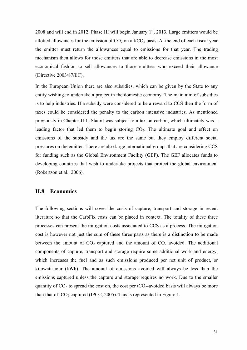
than that of tCO2 captured (IPCC, 2005). This is represented in Figure 1.

32

Figure 1: CO2 captured vs. CO2 avoided. (Source: IPCC, 2005)

The costs of capture and mitigation can also be found by the following formula:

Costavoided = [Costcaptured x CE] / [effnew / effold – (1-CE)] (3)

Where CE = fraction of CO2 captured; effnew = the efficiency of the power plant with

capture; effold = the efficiency of the power plant without capture (IEA, 2004). The

difference between the cost of capture and mitigation is largely dependent on the energy

efficiency penalty and as this factor decreases the two costs will begin to gravitate towards

each other.

When comparing a reference plant to a plant with capture it is common in academic

literature to compare similar plants, for example, a coal plant without capture to a coal

plant with capture. If a comparison were made to a coal plant with capture to a geothermal

power plant the emissions avoided would not seem very impressive as the emissions per

kWh are much lower in geothermal plants then coal plants.

Chapter II.8.1 compares costs between a coal reference plant and the same plant with

capture. If however, the marginal cost approach is taken in order to compare any two

plants with and without capture, regardless of the fuel source, the following formula could

be used:

MC = (COEcap – COEref) / (Eref – Ecap) (4)

33

Where the mitigation cost (MC) is found through the COEcap = cost of electricity of the

capture plant; COEref = cost of electricity of the reference plant; Eref = energy requirements

of the reference plant and Ecap = energy requirements of the capture plant.

II.8.1 Capture

Large sources of CO2 are industrial emitters such as fossil-fuel power plants, cement

treatment plants and oil and gas refineries (IPCC, 2005). The flue gas exiting the plant

contains CO2 from production although the content of CO2 in the gas varies according to

the source. In a coal-fired power plant the composition is of approximately 14% while a

natural gas fired plant may contain 3 to 4% (Holloway, 2005; IPCC, 2005). There are four

different routes that can be taken to capture a clean stream of CO2: capture from industrial

process streams, post-combustion capture, oxy-fuel combustion, and pre-combustion

capture (IPCC, 2005). The following section goes into detail on post-combustion capture

or the capture of CO2 from flue gases produced by fossil fuel combustion in order to make

the connection to the pulverized coal scenario in Chapter III.4.

One method of capture is the separation of CO2 through a chemical solvent and is currently

the common option. It has a capture efficiency of 85-90% (IPCC, 2005). The flue gas exits

the power plant and is then cooled before it comes into contact with the solvent and the

CO2 attaches. Once this is done the solvent is transported to a separate container where it is

manipulated in either pressure or temperature to release the CO2. The solvent is then

regenerated and free to be returned to the original vessel for reuse. Chemical solvents are

the best option when CO2 in the flue gas is at low concentrations such as less than 15%

(IEA, 2004).

A common chemical solvent is monoethanol amine (MEA), an amine-based solvent,

although others are available. The cost of the MEA is 1,25$/kg (Rao & Rubin, 2002). The

choice of solvent can be affected by the amount of by-products that form during use as

well as the decomposition rate (IPCC, 2005). The more by-products that are produced

increases the costs associated with cleanup and disposal, and the faster the solvent

decomposes leads to additional costs for replacement solvent. In some cases the by-

products and decomposed solvent can even be classified as hazardous waste and require

special disposal (Rao & Rubin, 2002).

34

Although MEA is the most commonly used amine there are competitors entering the

market as research and development is being completed. One such competitor is the KS1

amine developed by Mitsubishi and is being tested in various plants. One example is a coal

plant in Nagasaki, Japan where in 2006 10 tCO2 was captured per day (Oishi, 2006). The

KS1 solvent has a lower energy requirement and is not as vulnerable to degradation

leading to less waste but it is a more expensive solvent than MEA (Ho, Allinson & Wiley,

2009).

Sequestration requires that the gas be stripped of any additional species such as nitrogen

oxide (NOX), sulphur oxide (SOX) and other by-product gases in order for easier

compression and storage. The presence of these by-products can also have negative effects

on the solvent and decrease the ability for regeneration. Costs of capture generally include

the costs for compression, which changes the CO2 to a supercritical state making transport

easier and cheaper (Rubin, 2008).

The largest portion of the costs associated to capture is due to the energy penalty required

for regeneration of the solvent using heat as well as the steam necessary for stripping the

CO2 and compression of the subsequent stream (IPCC, 2005). The capture portion of CCS

can be quite energy intensive and can constitute an energy penalty of between 9 and 34%

(Aroonwilas & Veawab, 2007; Herzog, 1999). Post-combustion treatment is generally

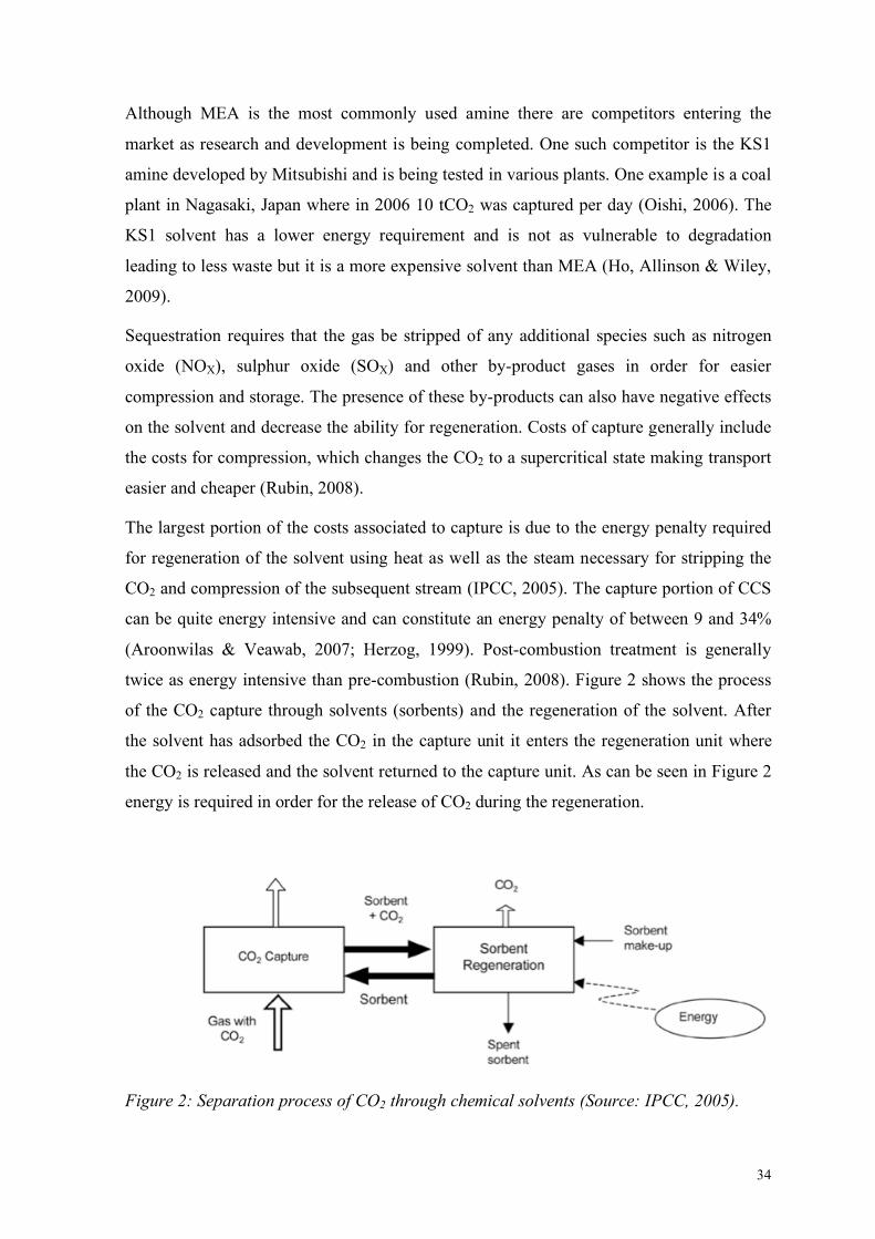
twice as energy intensive than pre-combustion (Rubin, 2008). Figure 2 shows the process

of the CO2 capture through solvents (sorbents) and the regeneration of the solvent. After

the solvent has adsorbed the CO2 in the capture unit it enters the regeneration unit where

the CO2 is released and the solvent returned to the capture unit. As can be seen in Figure 2

energy is required in order for the release of CO2 during the regeneration.

Figure 2: Separation process of CO2 through chemical solvents (Source: IPCC, 2005).

35

This capture technology can be retrofitted to existing fossil fuel plants. The disadvantages

are that the site may be constrained in the area available for additional equipment. Also,

the remaining plant life would need to be significant so that the high capital costs of the

capture equipment would be justified. Additionally, an older plant may have lower

efficiencies, which means the unavoidable energy penalty will have a greater effect on the

net output (IPCC, 2005). However an advantage is that the site, although perhaps not pre-

planned to include CCS, has an existing infrastructure and the facilities may be amortized

to a considerable degree. Also, they have a higher baseline of CO2 emissions compared to

new plants that may have lower emissions due to environmental pressures at the time of

design (Simbeck, 2001).

When considering the regions where plants, specifically coal-fired, may have substantial

life times left in order to justify retrofitting for capture technology, the United States may

have to wait until 2010-2020 to see any substantial actions. This is because the USA

peaked in its coal-fired generation construction around 1970 and since most plants have a

life of 40 to 50 years the remaining life of these plants should only average 2 to 12 years

(IEA, 2004). Some plants are being adapted to allow for better efficiency and this may

justify reanalyzing the capture retrofitting option as the plant may have an extended life-

time due to these changes in efficiency. However, Japan and China have only recently

begun building the main bulk of their coal-fired power plants and the average age is under

15 years of age making them optimum for retrofitting (IEA, 2004). The deployment of

CCS in China would be difficult to predict at this moment due to political uncertainty in

regards to emissions reductions.

Capital cost for capture generally includes the cost of the design, purchase and installation

of the capture system. The incremental cost is then the difference in capital cost between a

reference plant23 and the same plant with capture while producing the same amount of net

output on an MWe basis for example (IPCC, 2005). This then represents the amount of

additional capital needed in order to capture CO2. An additional comparison is the

incremental product cost in which the cost of electricity (COE) in $/kWh increases when

capture is added. The incremental COE gives an appropriate idea of what effect the capture

has on the cost of electricity. The COE can be found with the following equation:

23 A reference plant refers to a power generating plant with no capture and “business as usual” emissions.

36

COE = [(TCR)(FCF) + (FOM)] / [(CF)(8760)(kW)] + VOM + (HR)(FC) (5)

Where COE = levelized cost of electricity ($/kWh), TCR = total capital requirement ($),

FCF = fixed charge factor (fraction/yr), FOM = fixed operating costs ($/yr), CF = capacity

factor (fraction), 8760 = total hours in a typical year and kW = net plant power (kW),

VOM = variable operating costs ($/kWh), HR = net plant heat rate (kJ kWh-1), FC = unit

fuel cost ($/kJ), (IPCC, 2005). Using Equation 5 to calculate the COE of both a reference

plant and the plant with capture and comparing them can then give the incremental COE.

Equation 5 helps to explain why the economics of capture can sometimes seem bleak

especially when the energy penalty is considered. The energy is assumed to come from the

power plant itself. In Equation 5 the addition of capture means that the TCR is increasing

as well as the FOM and VOM. The kW in the denominator however is decreasing. Even if

the energy required for the capture were obtained elsewhere, outside of the plant, the unit

fuel cost would still increase. Overall the unit capital cost ($/kW) will increase and lead to

higher COE costs in ($/kWh). Cost is also dependent on the capacity factor of the plant and

the fixed charge rate (IPCC, 2005). The cost of the CO2 captured is represented in the

following equation:

$/tCO2 = [(COE)capture – (COE)ref] / (CO2, captured kWh-1) (6)

Where CO2, captured kWh-1 = total mass of CO2 captured (in tonnes) per net kWh (IPCC,

2005).

Costs for capture are in the range of US$ 18-72/tCO2 avoided (Herzog, 1999; David &

Herzog, 2001; IEA, 2004; Simbeck, 2001) and adds 44-87% to the capital costs of a plant,

$/kW (IPCC, 2005). Of the total costs for CCS the capture portion can contribute 83 to

93% (Rubin, 2008; Rubin, Chen & Rao, 2007). David (2000) compares four separate

pulverized coal (PC) plants and readjusts the economic evaluation to common factors such

as yearly operating hours, fixed charge factor and fuel prices to find that the range of the

incremental COE increase is 2,27 to 5,66 ¢/kWh.

Appendix A contains an adapted table from the IPCC that compared a compilation of

studies to illustrate the difference in cost of CO2 captured between studies and the resulting

range of US$ 23-35/tCO2 captured for new pulverized coal plants. This range is smaller

than the US$ 18-72 range cited from Herzog and others because as has already been

explained in Chapter II.8 the cost of capture on a tCO2 basis is always less than the cost of

tCO2 avoided. The highest and lowest values were taken for simplification purposes. If the

37

lowest value and highest value are studied more closely the same key elements are seen

leading to the difference in cost on a tCO2-captured basis. The highest case, a study by

Parsons in 2002 (as cited by IPCC, 2005) uses a reference plant with a much lower net

output (MWe) for the reference plant, 462 MWe, then the study conducted by the

International Energy Agency, (IEA GHG24), 758 MWe (2004). Also, the fixed charge

factor is much higher in the Parsons case, or 15,5% while the IEA GHG study uses 11,0%.

The capacity factor and the plant efficiency are also lower for the Parsons case. This

supports the notion that the cost of capture for new plants is sensitive to factors such as net

output or fixed charge factor as well as efficiency.

The following two columns in Appendix A show the lowest and highest costs for CO2

capture for existing pulverized coal plants. Both studies were conducted by Chen et al.

from 2003 (as cited by IPCC, 2005) and use relatively similar values for the two cases. The

capital cost has been fully amortized which does help to lower the COE. The lower case

constitutes an existing plant that adds an MEA capture system and has a higher capital cost

than the higher value case. However, the higher case assumes that instead of accessing the

required energy penalty internally that a natural gas boiler is added to compensate for this.

This leads to a higher fuel cost, as the natural gas must now be purchased in addition to the

coal. The capital costs are lower but the new fuel costs seem to be a sensitive factor when

existing plants are considered. The same technique of adding a natural gas boiler is

performed by Simbeck in 2001 in order to compensate for the additional energy needs.

While the IPCC compilation of reports shows incremental COE increases of between 1,8 to

4,6¢/kWh some later studies, such as by the IEA (2004), found that the COE increases

would be in the range of 1-2¢/kWh. When the results found by David (2000) are added,

which have already been mentioned, the resulting range in the literature can be from 1-

5,66¢/kWh. This is quite a large range and only accentuates the importance that plants

considering CCS must prepare their own analysis with the economical and technical

parameters that best fit their plant.

The IEA also projects that a coal plant starting operations in 2010 would see an

incremental cost of 775 US$/kW when capture is added while the same plant starting

operations in 2020 would only have an incremental cost of 695 US$/kW. This represents a

10% decrease in capital cost in $/kW basis while David and Herzog (2001) maintain that

24 Greenhouse Gas Research & Development Program

38

capital costs for capture could decline by as much as 33% by 2012 for a pulverized coal

plant. The cost range of 23 to 35 US$/tCO2 from the IPCC could also decline to as much as

10 to 25 US$/tCO2 according to the IEA (2004).

David (2000) through the study of the sensitivity of mitigation costs to technical and

economic variations found that the mitigations costs for a PC plant were most sensitive to

changes in the heat rate and energy requirement25. By decreasing the energy requirement

for capture by 10% the mitigation costs decreased by nearly 8% while a decrease of 10% in

the heat rate led to a decrease of mitigation costs by just over 4%. The least sensitive

factors were the operating and maintenance (O&M) costs as well as the incremental O&M.

There are, however, advancements being made that could possibly lower the capture costs.

As all technologies follow a learning curve26 the costs are expected to lower similarly, as

SOx scrubbers have done so through time (IPCC, 2005). The incremental COE and

mitigation costs could be reduced by 35% in 2012 when compared to 2000 (David, 2000).

Projects include advanced amines, chilled ammonia, and increased plant efficiency (Rubin,

2008). Perhaps the most promising option is sterically hindered amines that do not have as

strong of a bonding strength between the solvent and the CO2 and as such requires less

energy to release the CO2 from the solvent (IEA, 2004).

II.8.2 Transport

The most common method for transporting CO2 streams is by pipelines. The costs are

generally expressed in terms of US$/tCO2 captured. The major cost contributors are

construction costs, operations and maintenance and other costs that may include design,

insurance and right-of-way,27 (ROW) (IPCC, 2005). The cost of transport is dependent on

multiple factors including flow rate, diameter and distance. A report from the IEA (2004)

maintains that the cost is 1 to 5 US$/tCO2 transported per 100 km while Heddle, Herzog

and Klett (2003) find that when the flow is more than 10 Mt per year that the costs reach

economies of scale and are less than 1 US$/tCO2 per 100 km. These figures were then re-

examined and confirmed in 2006 by McCollum and Ogden.

25 The energy requirement can be illustrated by ER = EP/E where EP = energy penalty and E = emissions of CO2. 26 A phenomenon in which unit costs of technologies decrease as more units are produced. 27 ROW: The cost associated with the granting of land for transportation.

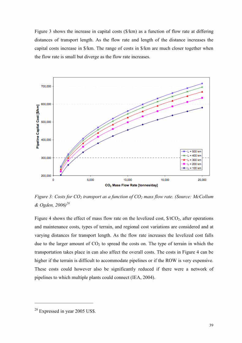
39

Figure 3 shows the increase in capital costs ($/km) as a function of flow rate at differing

distances of transport length. As the flow rate and length of the distance increases the

capital costs increase in $/km. The range of costs in $/km are much closer together when

the flow rate is small but diverge as the flow rate increases.

Figure 3: Costs for CO2 transport as a function of CO2 mass flow rate. (Source: McCollum

& Ogden, 2006)28

Figure 4 shows the effect of mass flow rate on the levelized cost, $/tCO2, after operations

and maintenance costs, types of terrain, and regional cost variations are considered and at

varying distances for transport length. As the flow rate increases the levelized cost falls

due to the larger amount of CO2 to spread the costs on. The type of terrain in which the

transportation takes place in can also affect the overall costs. The costs in Figure 4 can be

higher if the terrain is difficult to accommodate pipelines or if the ROW is very expensive.

These costs could however also be significantly reduced if there were a network of

pipelines to which multiple plants could connect (IEA, 2004).

28 Expressed in year 2005 US$.

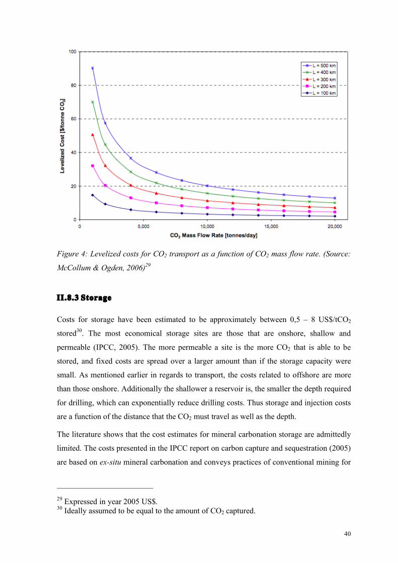
40

Figure 4: Levelized costs for CO2 transport as a function of CO2 mass flow rate. (Source:

McCollum & Ogden, 2006)29

II.8.3 Storage

Costs for storage have been estimated to be approximately between 0,5 – 8 US$/tCO2

stored30. The most economical storage sites are those that are onshore, shallow and

permeable (IPCC, 2005). The more permeable a site is the more CO2 that is able to be

stored, and fixed costs are spread over a larger amount than if the storage capacity were

small. As mentioned earlier in regards to transport, the costs related to offshore are more

than those onshore. Additionally the shallower a reservoir is, the smaller the depth required

for drilling, which can exponentially reduce drilling costs. Thus storage and injection costs

are a function of the distance that the CO2 must travel as well as the depth.

The literature shows that the cost estimates for mineral carbonation storage are admittedly

limited. The costs presented in the IPCC report on carbon capture and sequestration (2005)

are based on ex-situ mineral carbonation and conveys practices of conventional mining for

29 Expressed in year 2005 US$. 30 Ideally assumed to be equal to the amount of CO2 captured.

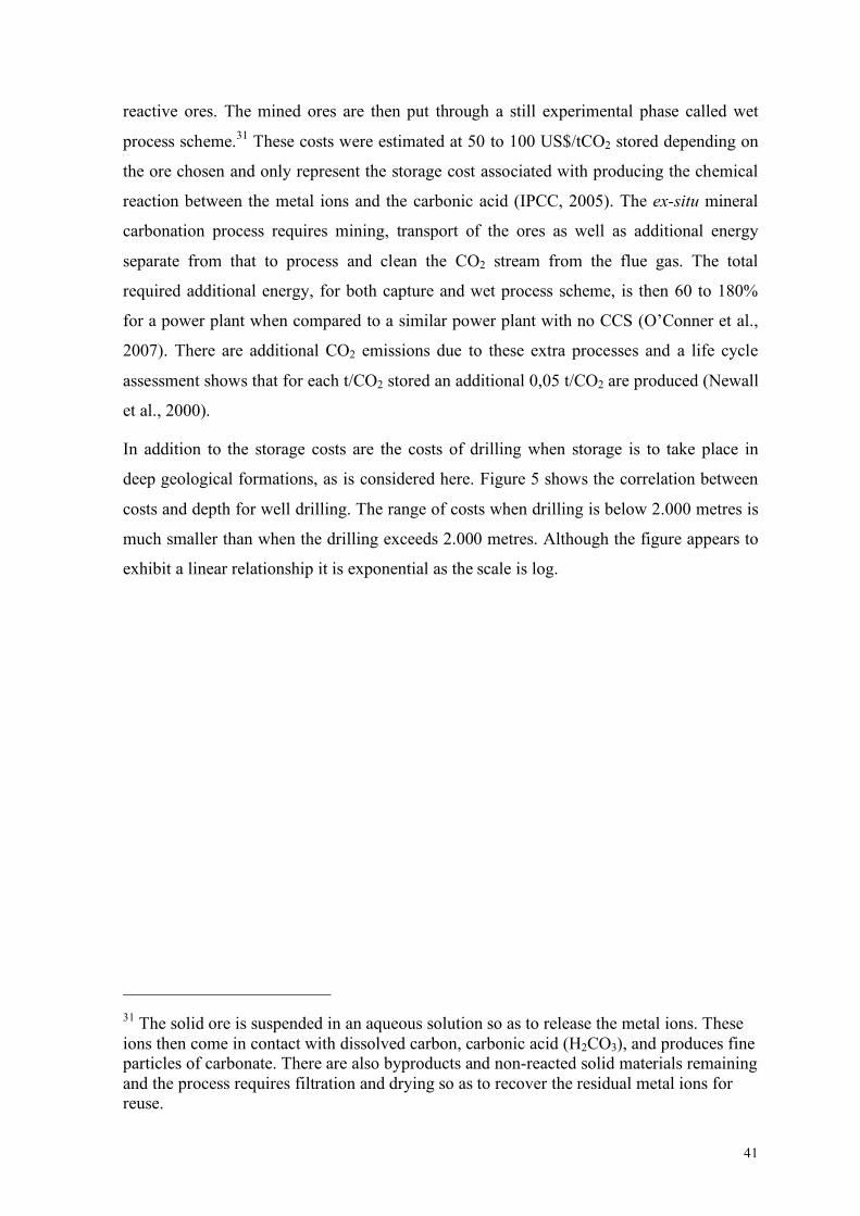
41

reactive ores. The mined ores are then put through a still experimental phase called wet

process scheme.31 These costs were estimated at 50 to 100 US$/tCO2 stored depending on

the ore chosen and only represent the storage cost associated with producing the chemical

reaction between the metal ions and the carbonic acid (IPCC, 2005). The ex-situ mineral

carbonation process requires mining, transport of the ores as well as additional energy

separate from that to process and clean the CO2 stream from the flue gas. The total

required additional energy, for both capture and wet process scheme, is then 60 to 180%

for a power plant when compared to a similar power plant with no CCS (O’Conner et al.,

2007). There are additional CO2 emissions due to these extra processes and a life cycle

assessment shows that for each t/CO2 stored an additional 0,05 t/CO2 are produced (Newall

et al., 2000).

In addition to the storage costs are the costs of drilling when storage is to take place in

deep geological formations, as is considered here. Figure 5 shows the correlation between

costs and depth for well drilling. The range of costs when drilling is below 2.000 metres is

much smaller than when the drilling exceeds 2.000 metres. Although the figure appears to

exhibit a linear relationship it is exponential as the scale is log.

31 The solid ore is suspended in an aqueous solution so as to release the metal ions. These ions then come in contact with dissolved carbon, carbonic acid (H2CO3), and produces fine particles of carbonate. There are also byproducts and non-reacted solid materials remaining and the process requires filtration and drying so as to recover the residual metal ions for reuse.

42

Figure 5: Well drilling cost as a function of depth. (Source: Heddle et al., 2003)

Site screening and selection is estimated to cost $1.685.00032 in order to screen and

evaluate the possibility of CO2 injection (Smith, 2001). This includes, as defined by Smith,

a definition of screening factors, collection of data describing the candidate area,

evaluating with respect to screening factors and preparing the final report to rank the site.

In order to evaluate the site multiple tasks must be undertaken including but not limited to:

installing sampling wells, analyzing samples, installing a test well and logging the

performance as well as site modelling and seismic evaluations.

II.8.4 Monitoring

Monitoring is essential in CCS programs to ensure there is no leakage as described in

Chapter II.4. Leakage in this paper refers to the limits set by Ha-Duong and Keith (2003)

where a leakage rate of less than 0,1% per year is considered to be perfect storage. This

limit can be found by considering future emissions, which are vital in calculating how long

storage is required. If it is possible to store CO2 for a time between 100 and 2.000 years

then the leakage rate can be between 0,01% and 1% (IEA, 2004). Zwaan and Gerlagh

(2009), as well as Hepple and Benson (2002), have confirmed this rate. Monitoring data is

limited but have been estimated to add 0,1-0,3 US$/tCO2 stored to the CCS total cost

(IPCC, 2005).

32 In 2001 US$.

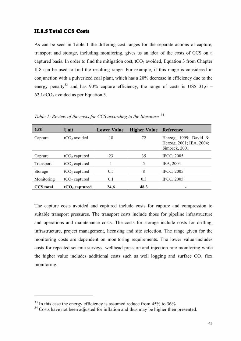
43

II.8.5 Total CCS Costs

As can be seen in Table 1 the differing cost ranges for the separate actions of capture,

transport and storage, including monitoring, gives us an idea of the costs of CCS on a

captured basis. In order to find the mitigation cost, tCO2 avoided, Equation 3 from Chapter

II.8 can be used to find the resulting range. For example, if this range is considered in

conjunction with a pulverized coal plant, which has a 20% decrease in efficiency due to the

energy penalty33 and has 90% capture efficiency, the range of costs is US$ 31,6 –

62,1/tCO2 avoided as per Equation 3.

Table 1: Review of the costs for CCS according to the literature. 34

USD Unit Lower Value Higher Value Reference Capture tCO2 avoided 18 72 Herzog, 1999; David &

Herzog, 2001; IEA, 2004; Simbeck, 2001

Capture tCO2 captured 23 35 IPCC, 2005

Transport tCO2 captured 1 5 IEA, 2004

Storage tCO2 captured 0,5 8 IPCC, 2005

Monitoring tCO2 captured 0,1 0,3 IPCC, 2005

CCS total tCO2 captured 24,6 48,3 -

The capture costs avoided and captured include costs for capture and compression to

suitable transport pressures. The transport costs include those for pipeline infrastructure

and operations and maintenance costs. The costs for storage include costs for drilling,

infrastructure, project management, licensing and site selection. The range given for the

monitoring costs are dependent on monitoring requirements. The lower value includes

costs for repeated seismic surveys, wellhead pressure and injection rate monitoring while

the higher value includes additional costs such as well logging and surface CO2 flex

monitoring.

33 In this case the energy efficiency is assumed reduce from 45% to 36%. 34 Costs have not been adjusted for inflation and thus may be higher then presented.

44

II.9 PESTLE Analysis

A tool that is often used to assess external risk factors is the PESTLE analysis. This

acronym stands for political, economic, socio, technical, legal and environmental analysis.

These six separate external influences can be the source of risk or opportunity for a firm as

well as a driving force in the market that the firm is trying to enter (McGee et al., 2005).

This analysis is used in combination with the SMART analysis explained in Chapter II.10,

to evaluate opportunities for CarbFix in the global marketplace. This type of analysis can

help not only to identify risks and opportunities today but also possible future business

environments. By being aware of the status of these external influences, such as the type of

political party currently in place in a country market, a firm is better able to minimize risk

events (Worthington & Britton, 2006).

Political factors are any actions by the government that may affect the behaviour or actions

of a firm. This could be in the form of taxes, regulations, subsidies to competitors and

many other actions (Cheverton, 2004). These can also be large and far-reaching impacts

such as the fall of a political party or commanding regime, or a complete country profile

overhaul such as the fall of the U.S.S.R. This could be the fall of the exchange rate and

thus less buying power of the household (Cheverton, 2004). All are external factors that

can affect the demand of the product or service of a firm.

Socio and cultural factors that can affect the demand of a product or service are an

important indication as to the cultural demographic of the market. This factor not only

lends to what type of products or services are demanded but also the values of the culture

(Cheverton, 2004). This can be for example the demand for ecologically friendly products

pointing towards a culture that is environmentally oriented. Technological factors are any

factors that can affect the production or use of a product or service not only in the firm

entering the market but also of the competitors (Cheverton, 2004).

Legal aspects of the PESTLE analysis cover laws and regulations in place that will affect

the business operations of a firm. Laws can affect the costs of a firm through employment

laws, production laws, and waste removal laws (Worthington & Britton, 2006). The more

stringent the laws the more costs can be accrued due to actions that the firm may not have

undertaken in the absence of the law. Environmental factors can range from resources that

are readily or scarcely available that may be required for production to weather patterns

45

and harsh weather climates that may hinder regular business actions such as transport

(Cheverton, 2004).

II.10 Simple Multi-Attribute Rating Technique

The SMART analysis is based on the preferences of a decision maker. It is a prescriptive

analysis that describes the alternative best chosen when the decision maker behaves in

accordance to preferences (Goodwin & Wright, 2004). This type of analysis is commonly

used where the level of uncertainty is low or information is readily available. Information

can be in the form of known costs or through proxies35, which describe a certain attribute

in a quantitative manner (Goodwin & Wright, 2004). The analysis provides the decision

maker with the correct course of action to take where multiple alternatives were present.

Before being able to employ the SMART analysis an objective must be set out and is

determined to be the goal met by the decision determined through SMART. Attributes are

then the performance of factors that can help achieve this predetermined objective and the

score determined to be the value (Edwards, 1971). There are then 8 stages of the analysis

as described in the following (Goodwin & Wright, 2004).

• The first stage is to determine the decision maker.

• The second stage is to determine all the alternative avenues available to meet the

predetermined objective.

• The third stage is to identify and define those attributes that can affect the choice of

alternative.

• The fourth stage involves assigning a quantitative value to each identified attribute.

This may be done through proxies.

• The fifth stage is to determine the weight of each attribute. This is a key stage and

determines how important each attribute is.

• The sixth stage is to find the weighted average of the values that have been given to

each attribute. The weighted average is found by multiplying the weight of an

attribute by its value.

35 An attribute which may not be directly related but be a descriptive representative.

46

• The seventh stage is to analyze the results of the aggregate scores. The aggregate

score is found by summing all of the weighted averages of all of the benefits for

one decision alternative.

• The eighth stage is generally a sensitivity analysis to determine how sensitive the

final decision path is to changes in values.

47

III. TECHNO-ECONOMIC SCENARIOS

III.1 CarbFix – Present Status & Methodology

CarbFix is a pilot study being performed at the Hellisheidi geothermal power plant area

located in southwest Iceland. It was launched September 29th, 2007 and is a cooperation

between four partners: Reykjavik Energy (OR), University of Iceland36, University of

Columbia37 and the Centre National de la Recherche Scientifique in Toulouse, France. The

goal of the CarbFix pilot program is to test the in-situ sequestration of carbon dioxide

(CO2) through mineral carbonation in basalt. The project will develop industrial methods

of CO2 storage in basaltic rock. The project consists of field scale injection of water-

saturated CO2 into basalt, laboratory experiments, geochemical modelling and natural CO2

water analogues. Through this program considerable expertise and knowledge are built up

in order to continue advancing science for CO2 storage in basalt.

The Hellisheidi power plant is a geothermal plant that currently has a capacity of 213 MWe

but is due to be extended to 303 MWe (Reykjavik Energy, 2009). It produces

approximately 60.000 tCO2 per year (Gislason et al., 2009) but with the future increases in

production this will reach approximately 90.000 tCO238. The CO2 emissions combined

with hydrogen sulphide (H2S), hydrogen (H2), nitrogen (N2), methane (CH4) and oxygen

(O2) make up the geothermal non-condensable gas, which is present in the geothermal

steam (Gislason et al., 2009). They are drawn up from the produced fluids from wells and

are discharged to atmosphere. The composition of the gas is mainly carbon dioxide, or

83% of mass, while the hydrogen sulphide is 16% and the remaining elements combined

make up 1% of the gas (Matter et al., 2008).

In the 2008 Environmental Report from Reykjavík Energy the hydrogen sulphide

emissions are discussed and a project proposed to reduce these emissions from the Hengill

36 Institute of Earth Sciences 37 Earth Institute – Lamont-Doherty Earth Observatory

48

area, where the Hellisheidi geothermal plant is located. This would be accomplished by

separating the H2S from the geothermal gas, mixing it with water and re-injecting into the

ground. This program, like CarbFix, is in its initial research stages. After this process the

stream from the H2S abatement system is an almost pure stream of CO2. CarbFix then has

a unique opportunity to use this pure stream to test re-injection and mineral carbonation of

CO2.

III.1.1 H2S Abatement System

The resulting flow from the abatement system is a compressed and cooled gas containing

98% CO2 and 2% H2S (Matter et al., 2008). It is then transported to the injection site by a

3-kilometer long HDPE pipeline (Sigurdardottir, 2009).

The costs of the abatement system were not included in the profitability analysis of this

thesis, as they are regarded as a sunk cost39. The H2S abatement is a separate project from

CarbFix and would be performed regardless of the CarbFix status. The author did want to

provide some of the costs and energy requirements that this process entails for reference.

Although the literature costs have been given in US$, all of the following cost analysis will

be in Euros, !.

The capture efficiency describes how much of the gas coming through the abatement

system is actually cleaned and ready for pipe-end use. As there are always some losses as

well as downtime in the system for operations and maintenance an efficiency of 95% has

been used here. This also corresponds to the average capacity factor of a geothermal plant.

As the pilot program research continues the capture efficiency may change. Thus streams

from the pilot project, 0,07 kg/s, and also from a full-scale scenario, 1,9 kg/s, would be

scaled down to 0,067 kg/s and 1,8 kg/s respectively.

The abatement system requires some internal energy use by the Hellisheidi plant in order

to separate and compress the gas stream from the geothermal steam. The equipment costs

for the pilot program were approximately 0,58 million Euros while the electrical

38 Calculations based on CO2 emissions by sector as published by Bloomfield, Moore & Neilson, 2003. 39 Costs that cannot be recovered once they have been incurred.

49

requirement yielded a yearly cost of 0,05 million Euros. The electricity costs are based on

an energy requirement of 173 kW and a cost of electricity of 0,036 !/kWh40.

The cost of the abatement system was also analyzed based on a full-scale scenario, in

which all of the geothermal gas from Hellisheidi would be processed through the system

and subsequently sequestered using the CarbFix method. The total capital costs and

electrical requirements were scaled41 and increased to 4,17 million Euros and the

electricity cost to 1,02 million Euros per year. The energy requirements were scaled from

173 kW to 3,4 MW.

III.1.2 Basalt

Basalt is an igneous rock that can be present as glassy or crystalline. It contains calcium

oxide (CaO), which is a key element of mineral carbonation (Sigurdardottir, 2008). A

reaction between the CO2 and the calcium present produces calcite (CaCO3), which is a

stable geological formation and has a small of risk of leakage (Oelkers & Cole, 2008;

Gislason et al., 2009)). More than 90% of Iceland’s bedrock is basaltic (Sigurdardottir,

2008) but basalt makes up less than 10% of the Earth’s crust (Gislason et al., 2009).

Although 10% may seem like a small percentage, that portion of the crust does an

incredible amount of work to reduce atmospheric CO2, as approximately 33% of the CO2

consumed through natural weathering is done so by basalt (Oelkers et al., 2008).

Using the basalt present towards the mineral carbonation process does have some

requirements and challenges. There are water requirements for re-injection that must be

met as well as the presence of a cap rock in order to prevent leakage. The cap rock helps to

keep the dissolved CO2 in contact with the basalt for a sufficient time in order for the

carbon mineralization to take place (Oelkers et al., 2008). However, this may prove in the

future to not be absolutely required. This is due to the nature of the water when it has been

mixed with CO2. While supercritical CO2 is buoyant and lighter than the water present in

the geological formation, water-saturated CO2 is heavier and thus would tend to sink (S.R.

Gislason, personal communication, October 23, 2009).

40 This cost is found by referring to Reykjavík Energy’s stated prices at http://www.or.is/Fyrirtaeki/Verdskraogskilmalar/Rafmagn/ given in ISK and exchanged to Euros. Prices accessed May 2009 and may have changed. 41 The equation is explained in detail in Chapter III.3 and is listed as Equation 7.

50

III.1.3 CarbFix methodology

The CarbFix method begins after the H2S abatement system has produced a clean stream of

CO2. The site for re-injection is approximately 3 km south of the Hellisheidi power plant.

The water requirement, as described by Gislason et al. (2009), maintains that for each kg/s

of CO2 flow there is a need for 27 litres/second (l/s) when the water temperature is at 19°C.

While dry CO2 could be injected, the mineral carbonation process would be expected to be

slower as the CO2 would need to react with the groundwater (Matter et al., 2008). This

could ultimately allow for a higher possibility of leakage. Water from well HN-1 is

pumped to the injection well HN-2 where it flows into an injection pipe. The CO2 gas is

piped from the H2S abatement system and will continue down the well HN-2 inside the

injection pipe. At a suitable depth the CO2 will be dissolved in the water. The injection

pipe leads the water containing the dissolved CO2 down to a depth where it reaches the

basaltic rock. The temperature at this depth is between 30°C and 50°C (Matter et al.,

2008).

Tracers42 are added for monitoring the fate of the injected CO2 in the subsurface (Gislason

et al., 2009). The gas stream of CO2 is piped from the abatement system to well HN-2, the

re-injection well, through a plastic pipeline. The delivery pressure from the abatement

system, 30 bar, is sufficient so no further pressurization is needed.

The area for re-injection is estimated to be 3 kilometres (km) long, 1.500 m wide and 600

m thick (Aradottir, Sonnenthal, Bjornsson, Gunnlaugsson, & Jonsson, 2009). As

mentioned in Chapter II.2, Gislason et al. (2009) estimate that the volume of this target

area can accommodate 12 Mt of CO2. To give a clear picture of how much this is the

current total yearly CO2 stream from Hellisheidi is 60.000 tonnes and as such, this area

would accommodate 200 years of re-injection.

Figure 6 shows the layout of the wells HN-2 and HN-1 as well as the monitoring wells.

The wells, HN-1 (water) and HN-2 (injection well), are identified within the boxes.

Multiple monitoring wells in conjunction with the tracers will allow for reservoir

monitoring as well as the aquifer along the hydraulic gradient (Matter et al., 2008). The

deep monitoring wells are marked by HN-4, HK-34, HK-31 and HK-26 and the shallow

42 Tracers are the injection of chemicals into systems in order to assess the recovery during various times and at multiple observation points, in this case the monitoring wells (Khalilabad, Axelsson & Gislason, 2008).

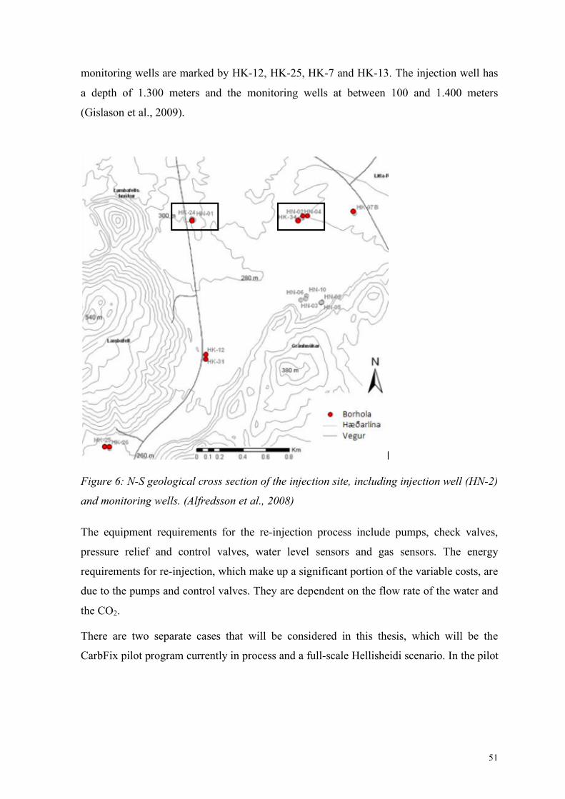
51

monitoring wells are marked by HK-12, HK-25, HK-7 and HK-13. The injection well has

a depth of 1.300 meters and the monitoring wells at between 100 and 1.400 meters

(Gislason et al., 2009).

Figure 6: N-S geological cross section of the injection site, including injection well (HN-2)

and monitoring wells. (Alfredsson et al., 2008)

The equipment requirements for the re-injection process include pumps, check valves,

pressure relief and control valves, water level sensors and gas sensors. The energy

requirements for re-injection, which make up a significant portion of the variable costs, are

due to the pumps and control valves. They are dependent on the flow rate of the water and

the CO2.

There are two separate cases that will be considered in this thesis, which will be the

CarbFix pilot program currently in process and a full-scale Hellisheidi scenario. In the pilot

52

program the aim is to inject CO2 at a rate of 0,067 kg/s43 with approximately 2 l/s of water.

This would be a total of 2.100 tCO2 per year. The full-scale project would however, if

undertaken in the future, inject at a rate of 1,8 kg/s and sequester a total of 57.000 tonnes

per year.

III.2 CarbFix Pilot Program

The following section details the costs and economic parameters of the CarbFix pilot

program. The purpose of the pilot program is to test the storage abilities of basalt. Should

the sequestration prove to be a long-term solution a decision will be made whether to

continue on a full scale. Understanding the key cost drivers of this process will not only

help to make an informed decision but also signify what areas need more focus in order for

this to be economical.

It is also important to note that the following section does not review the costs of the

capture system, as that is a sunken cost. Please refer to Chapter III.1.1 for a review of the

H2S abatement plant, which acts as a capture system in this process.

III.2.1 Data

The capital costs were given to a certain degree of uncertainty. A three-point method44

with 95% confidence interval was used and the resulting costs used in the application of

the cost analysis. Table 2 shows the most likely cost that was given and the applied cost

after the three-point method. The monitoring wells total 9 and each well has a cost of 0,3

million Euros while the site screening costs were directly referenced from Simbeck (2001)

and adjusted for inflation.

43 This is the injection rate of 0,07 kg/s after a capture efficiency limitation has been applied as was discussed in Chapter III.1.1. 44 The three-point method is a statistical estimation technique based on the normal distribution. Three estimates are used (best case, most likely case, worst case) with a confidence interval in order to find an estimation of the applied cost.

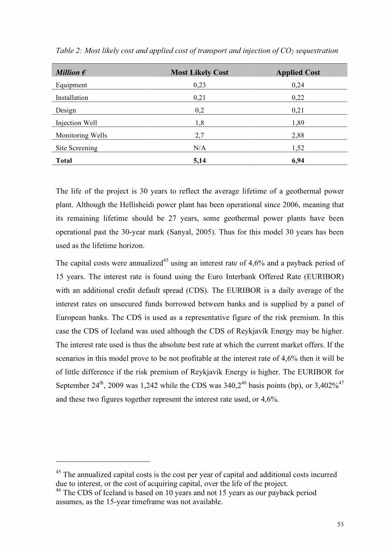
53

Table 2: Most likely cost and applied cost of transport and injection of CO2 sequestration

Million ! Most Likely Cost Applied Cost Equipment 0,23 0,24

Installation 0,21 0,22

Design 0,2 0,21

Injection Well 1,8 1,89

Monitoring Wells 2,7 2,88

Site Screening N/A 1,52

Total 5,14 6,94

The life of the project is 30 years to reflect the average lifetime of a geothermal power

plant. Although the Hellisheidi power plant has been operational since 2006, meaning that

its remaining lifetime should be 27 years, some geothermal power plants have been

operational past the 30-year mark (Sanyal, 2005). Thus for this model 30 years has been

used as the lifetime horizon.

The capital costs were annualized45 using an interest rate of 4,6% and a payback period of

15 years. The interest rate is found using the Euro Interbank Offered Rate (EURIBOR)

with an additional credit default spread (CDS). The EURIBOR is a daily average of the

interest rates on unsecured funds borrowed between banks and is supplied by a panel of

European banks. The CDS is used as a representative figure of the risk premium. In this

case the CDS of Iceland was used although the CDS of Reykjavík Energy may be higher.

The interest rate used is thus the absolute best rate at which the current market offers. If the

scenarios in this model prove to be not profitable at the interest rate of 4,6% then it will be

of little difference if the risk premium of Reykjavík Energy is higher. The EURIBOR for

September 24th, 2009 was 1,242 while the CDS was 340,246 basis points (bp), or 3,402%47

and these two figures together represent the interest rate used, or 4,6%.

45 The annualized capital costs is the cost per year of capital and additional costs incurred due to interest, or the cost of acquiring capital, over the life of the project. 46 The CDS of Iceland is based on 10 years and not 15 years as our payback period assumes, as the 15-year timeframe was not available.

54

The resulting annualized capital costs were 0,65 M!. As some of the costs were given in

varying currencies the following exchange rates were used according to the 2009 averages

from January to June: ISK48/US$ = 124; EUR/US$ = 0,74; ISK/EUR = 166. These

exchange rates are constant throughout Chapters III.3 and III.4 as well. The operating and

maintenance costs were calculated by using a factor of 0,02549 of the capital costs for the

equipment, injection wells and monitoring wells resulting in a yearly cost of 0,13 M!.

The remaining costs are CO2 flow dependent of the stream exiting the H2S abatement

system as well as on the flow of the water. In the pilot program the flow entering the

abatement system is 0,07 kg/s but due to capture efficiencies, 95%, has been reduced to

0,067 kg/s. The water requirement is 27 l/s for each kg/s of CO2, which results in a yearly

water requirement of 56.6 million litres. The water costs were calculated to be 0,0001

!/litre50 which gives a yearly cost of 0,008 M!.

The energy requirement for the transportation and injection is approximately 200 kW. This

is split up between pumping, 15 kW and support systems, 185 kW. Using an electricity

cost of 0,036 !/kWh and a capacity factor of 95% the yearly costs were 0,06 M!. It is

assumed that pumping energy requirements will scale linearly with flow rates and support

system power consumption is fixed to a certain degree.

Monitoring

The remaining cost is monitoring for CO2 leakage and other environmental damages.

There are many different techniques available. Specific regulatory requirements have yet to

47 Although the currency exchange rates are based on the averages of January to June of 2009 this is not the same method used representative figure for the CDS. This is because the CDS on September 24th of 2008 was 340bp, the same as the date used for this year. Additionally, before the September 24th date of 2008 the point spread was fairly stable. The average from January to June resulted in 728bp, a much higher figure. Thus we can assume that the CDS has followed a bell curve from September of 2008 until 2009 and a hypothesis can be made that it is perhaps finding market equilibrium once again. 48 Icelandic Krona 49 The O&M factor takes into account the labor costs of injection. This is slightly lower than the 3% factor used for capture in literature as there is no solvent to renew or waste to dispose of. It is also lower than the 3% factor used for transport, as the CarbFix method of transportation does not employ the use of booster stations (Neele, Hendriks, Brandsma, & Blomen, 2009). 50 This cost is found by referring to Reykjavík Energy’s stated prices at http://www.or.is/Fyrirtaeki/Verdskraogskilmalar/Kaltvatn/ given in ISK and exchanged to Euros. Prices accessed May, 2009 and may have changed.

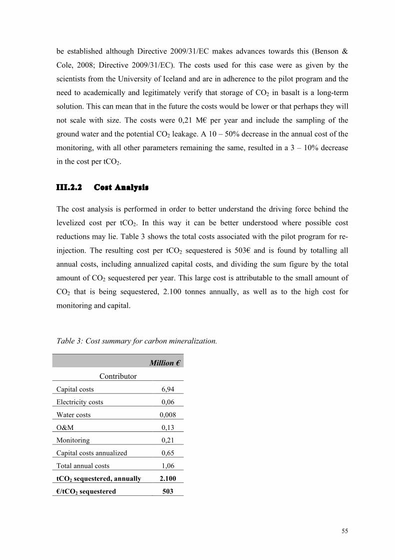
55

be established although Directive 2009/31/EC makes advances towards this (Benson &

Cole, 2008; Directive 2009/31/EC). The costs used for this case were as given by the

scientists from the University of Iceland and are in adherence to the pilot program and the

need to academically and legitimately verify that storage of CO2 in basalt is a long-term

solution. This can mean that in the future the costs would be lower or that perhaps they will

not scale with size. The costs were 0,21 M! per year and include the sampling of the

ground water and the potential CO2 leakage. A 10 – 50% decrease in the annual cost of the

monitoring, with all other parameters remaining the same, resulted in a 3 – 10% decrease

in the cost per tCO2.

III.2.2 Cost Analysis

The cost analysis is performed in order to better understand the driving force behind the

levelized cost per tCO2. In this way it can be better understood where possible cost

reductions may lie. Table 3 shows the total costs associated with the pilot program for re-

injection. The resulting cost per tCO2 sequestered is 503! and is found by totalling all

annual costs, including annualized capital costs, and dividing the sum figure by the total

amount of CO2 sequestered per year. This large cost is attributable to the small amount of

CO2 that is being sequestered, 2.100 tonnes annually, as well as to the high cost for

monitoring and capital.

Table 3: Cost summary for carbon mineralization.

Million ! Contributor

Capital costs 6,94

Electricity costs 0,06

Water costs 0,008

O&M 0,13

Monitoring 0,21

Capital costs annualized 0,65

Total annual costs 1,06

tCO2 sequestered, annually 2.100

!/tCO2 sequestered 503

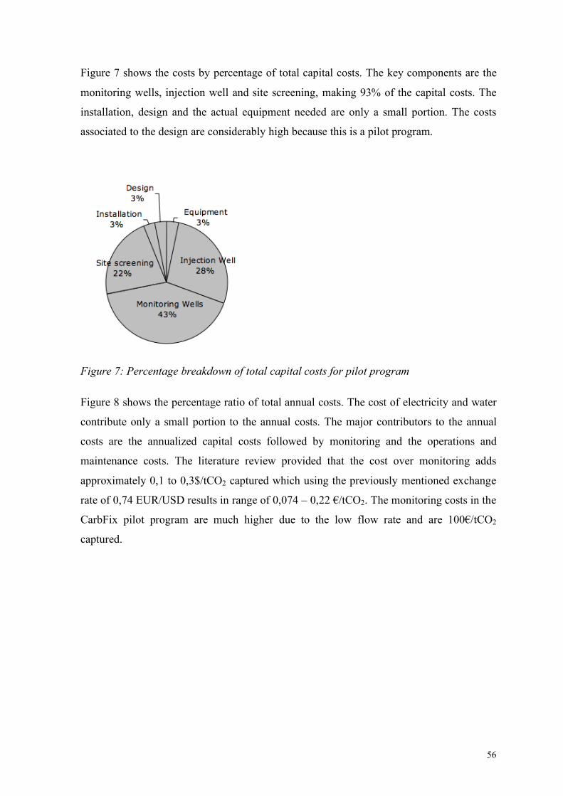
56

Figure 7 shows the costs by percentage of total capital costs. The key components are the

monitoring wells, injection well and site screening, making 93% of the capital costs. The

installation, design and the actual equipment needed are only a small portion. The costs

associated to the design are considerably high because this is a pilot program.

Figure 7: Percentage breakdown of total capital costs for pilot program

Figure 8 shows the percentage ratio of total annual costs. The cost of electricity and water

contribute only a small portion to the annual costs. The major contributors to the annual

costs are the annualized capital costs followed by monitoring and the operations and

maintenance costs. The literature review provided that the cost over monitoring adds

approximately 0,1 to 0,3$/tCO2 captured which using the previously mentioned exchange

rate of 0,74 EUR/USD results in range of 0,074 – 0,22 !/tCO2. The monitoring costs in the

CarbFix pilot program are much higher due to the low flow rate and are 100!/tCO2

captured.

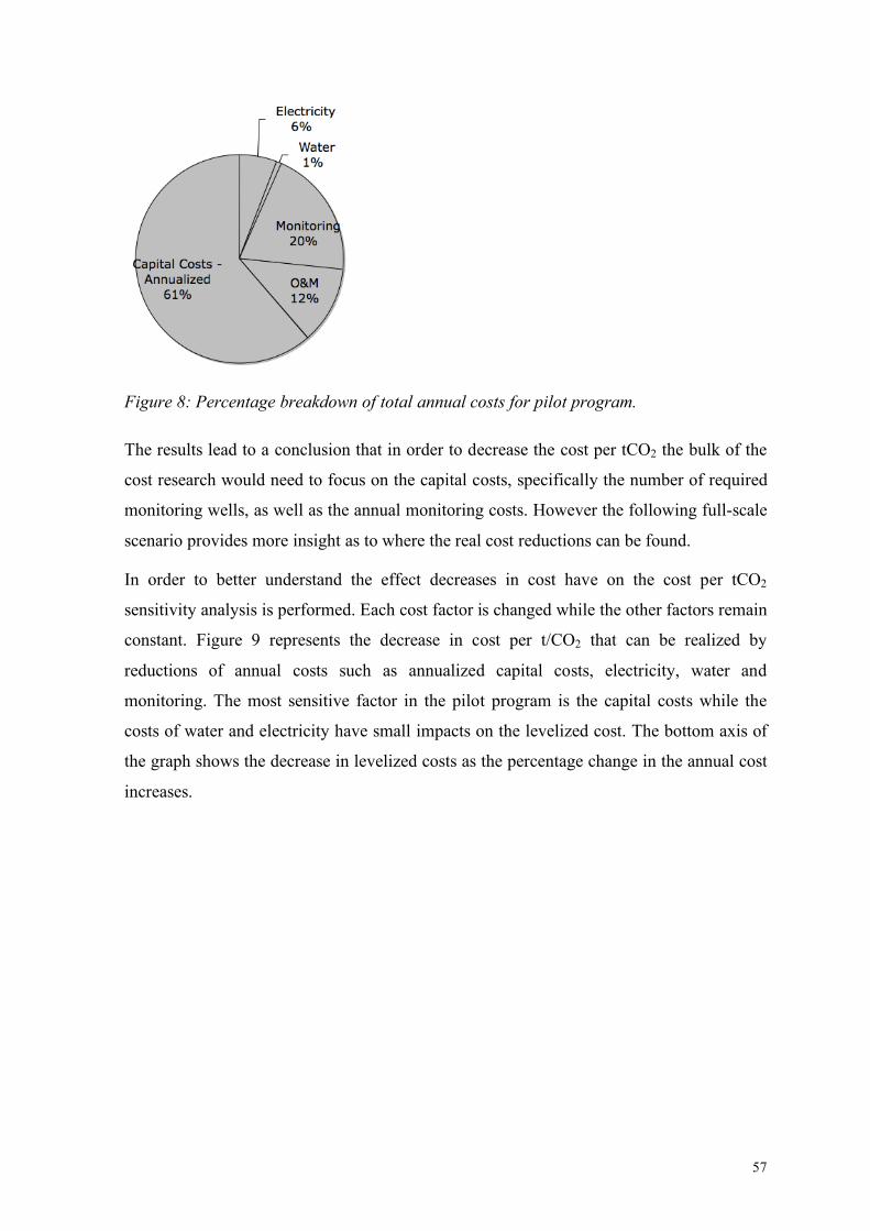
57

Figure 8: Percentage breakdown of total annual costs for pilot program.

The results lead to a conclusion that in order to decrease the cost per tCO2 the bulk of the

cost research would need to focus on the capital costs, specifically the number of required

monitoring wells, as well as the annual monitoring costs. However the following full-scale

scenario provides more insight as to where the real cost reductions can be found.

In order to better understand the effect decreases in cost have on the cost per tCO2

sensitivity analysis is performed. Each cost factor is changed while the other factors remain

constant. Figure 9 represents the decrease in cost per t/CO2 that can be realized by

reductions of annual costs such as annualized capital costs, electricity, water and

monitoring. The most sensitive factor in the pilot program is the capital costs while the

costs of water and electricity have small impacts on the levelized cost. The bottom axis of

the graph shows the decrease in levelized costs as the percentage change in the annual cost

increases.

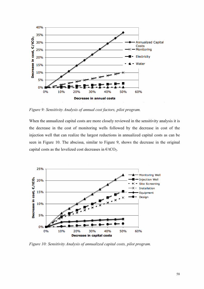
58

Figure 9: Sensitivity Analysis of annual cost factors, pilot program.

When the annualized capital costs are more closely reviewed in the sensitivity analysis it is

the decrease in the cost of monitoring wells followed by the decrease in cost of the

injection well that can realize the largest reductions in annualized capital costs as can be

seen in Figure 10. The abscissa, similar to Figure 9, shows the decrease in the original

capital costs as the levelized cost decreases in !/tCO2.

Figure 10: Sensitivity Analysis of annualized capital costs, pilot program.

59

A Monte Carlo simulation51 on the CarbFix pilot program and a range of possible capital

costs provides additional information. The simulation includes 5,000 runs and the capital

costs assumed to follow a normal distribution. The mean of the simulation is 486 !/tCO2

while 90% of the events are between 456 and 515 !/tCO2.

III.2.3 Profitability Assessment

The profitability assessment performed on the pilot program is done to find what the price

of mitigation would need to be in order for the system to realize a reasonable return. This

could be through the form of a trading price on the carbon market or carbon dioxide

emissions tax imposed by the government. As the costs are high and the captured amount

of CO2 low the profitability assessment returns quite high figures for a needed price per

tCO2.

The key profitability ratios and figures that were looked at were the following: Debts-to-

Capital ratio (D/C), Return-on-Equity ratio (ROE), the internal rate of return (IRR), the net

present value (NPV) of the net cash flow and the net profit or loss over the project life. The

D/C ratio helps us to understand the financial strength of the project. The higher the ratio

the more debt there is than capital and thus the higher chance of default due to the weight

of those debts. There are varying versions of this ratio and so it is important to point out

that the debts here are considered to be the short and long term debts while the capital is

the net profit and the shareholder equity. The ROE shows the income that is generated with

shareholder money and is the profit after tax in ratio to the total capital at a given time.

The NPV is a consideration of the future cash flows when the time value of money is taken

into account. It is dependent on the discount factor used and the risk level of the project.

The IRR is the rate at which the NPV is equal to zero and projects are usually considered

acceptable when the IRR is higher than the minimum acceptable rate of return (MARR)

given by a company or shareholders, in this case 15%.

Additionally, the net profit (loss) over the project life is considered. It is the profit after tax

after deductions have been made for payable dividends. All of the ratios and figures

considered in the profitability assessments, with the exception of the net profit (loss), are

51 Monte Carlo simulation is a mathematical and computer based model in which multiple combinations of factors are generated to find the probability that a specific outcome will happen (Goodwin & Wright, 2004).

60

for year 8 giving the project sufficient time to progress and giving a deadline for which to

begin to show financial promise. The net profit (loss) figure is calculated using the full life

of the project, or 30 years.

The economic parameters used in all of the profitability assessments discussed are the

following, in addition to the capital costs and variable costs discussed in preceding section:

Table 4: Economic parameters used for profitability assessment of the CarbFix pilot

program.

Economic Parameters Variable cost, !/tCO2 32,5

Fixed cost, M!/year 0,34

Time horizon, years 30

Loan interest rate, % 4,6

Payback period, years 15

Working capital, M! 0,18

Discount rate, % 15

Loan management fee, % 2

Income tax, % 15

Depreciation rates, % Equipment 5

Injection wells 15

Monitoring wells 15

Other 20

The initial price is 900!/tCO2 avoided, approximately 97% higher than the cost, which

means that if the selling price in the trading market were to be 900 ! per tonne then the

sequestration at Hellisheidi and its resulting trading permits would realize a certain profit

per year. Similarly, if the tax is 900 !/tCO2 emitted then the profit can be assumed to be a

saved cost. While all aspects of the profitability analysis will be covered, it is clear this will

not be economical.

Figure 11 represents the progression of the NPV of the total and net cash flows through the

life of the project. The net cash flow becomes positive at year 4, 2013, while the total cash

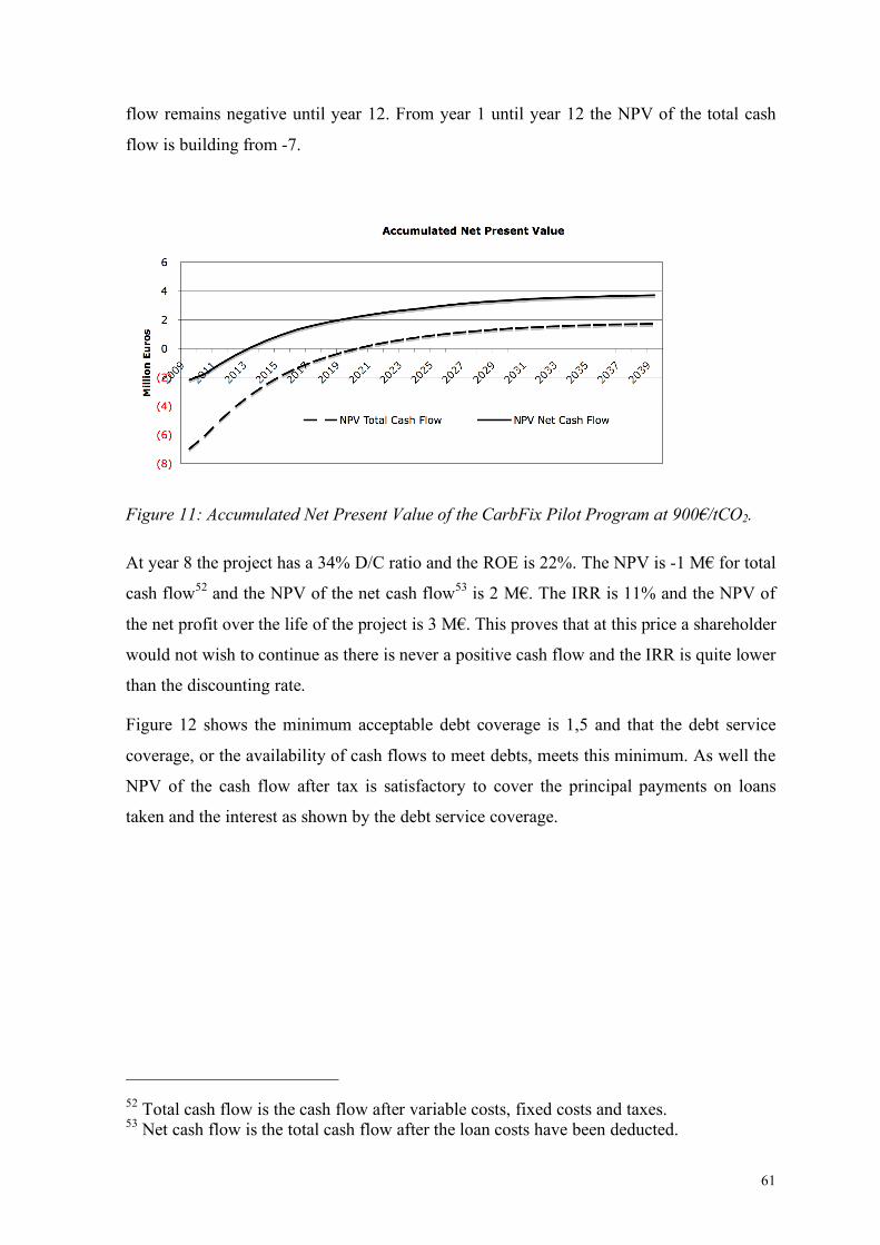
61

flow remains negative until year 12. From year 1 until year 12 the NPV of the total cash

flow is building from -7.

Figure 11: Accumulated Net Present Value of the CarbFix Pilot Program at 900!/tCO2.

At year 8 the project has a 34% D/C ratio and the ROE is 22%. The NPV is -1 M! for total

cash flow52 and the NPV of the net cash flow53 is 2 M!. The IRR is 11% and the NPV of

the net profit over the life of the project is 3 M!. This proves that at this price a shareholder

would not wish to continue as there is never a positive cash flow and the IRR is quite lower

than the discounting rate.

Figure 12 shows the minimum acceptable debt coverage is 1,5 and that the debt service

coverage, or the availability of cash flows to meet debts, meets this minimum. As well the

NPV of the cash flow after tax is satisfactory to cover the principal payments on loans

taken and the interest as shown by the debt service coverage.

52 Total cash flow is the cash flow after variable costs, fixed costs and taxes. 53 Net cash flow is the total cash flow after the loan costs have been deducted.

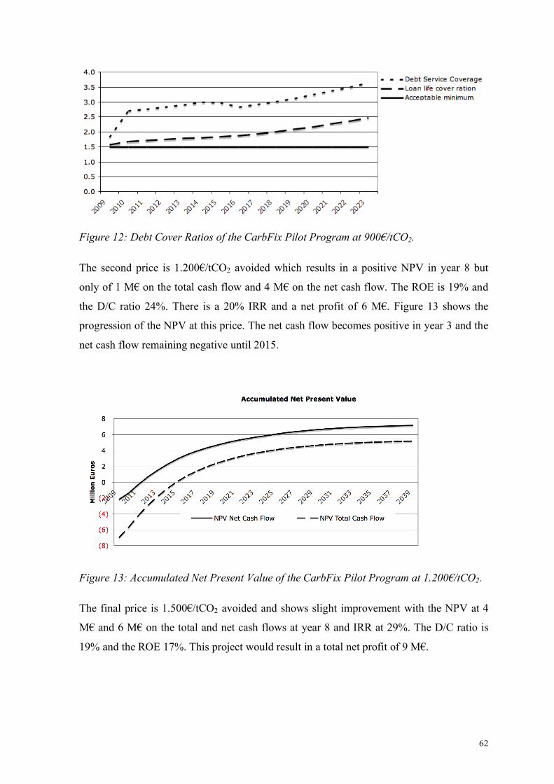
62

Figure 12: Debt Cover Ratios of the CarbFix Pilot Program at 900!/tCO2.

The second price is 1.200!/tCO2 avoided which results in a positive NPV in year 8 but

only of 1 M! on the total cash flow and 4 M! on the net cash flow. The ROE is 19% and

the D/C ratio 24%. There is a 20% IRR and a net profit of 6 M!. Figure 13 shows the

progression of the NPV at this price. The net cash flow becomes positive in year 3 and the

net cash flow remaining negative until 2015.

Figure 13: Accumulated Net Present Value of the CarbFix Pilot Program at 1.200!/tCO2.

The final price is 1.500!/tCO2 avoided and shows slight improvement with the NPV at 4

M! and 6 M! on the total and net cash flows at year 8 and IRR at 29%. The D/C ratio is

19% and the ROE 17%. This project would result in a total net profit of 9 M!.

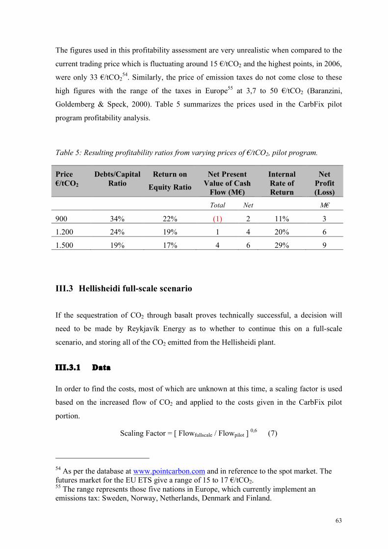
63

The figures used in this profitability assessment are very unrealistic when compared to the

current trading price which is fluctuating around 15 !/tCO2 and the highest points, in 2006,

were only 33 !/tCO254. Similarly, the price of emission taxes do not come close to these

high figures with the range of the taxes in Europe55 at 3,7 to 50 !/tCO2 (Baranzini,

Goldemberg & Speck, 2000). Table 5 summarizes the prices used in the CarbFix pilot

program profitability analysis.

Table 5: Resulting profitability ratios from varying prices of !/tCO2, pilot program.

Price !/tCO2

Debts/Capital Ratio

Return on Equity Ratio

Net Present Value of Cash

Flow (M!)

Internal Rate of Return

Net Profit (Loss)

Total Net M!

900 34% 22% (1) 2 11% 3

1.200 24% 19% 1 4 20% 6

1.500 19% 17% 4 6 29% 9

III.3 Hellisheidi full-scale scenario

If the sequestration of CO2 through basalt proves technically successful, a decision will

need to be made by Reykjavík Energy as to whether to continue this on a full-scale

scenario, and storing all of the CO2 emitted from the Hellisheidi plant.

III.3.1 Data

In order to find the costs, most of which are unknown at this time, a scaling factor is used

based on the increased flow of CO2 and applied to the costs given in the CarbFix pilot

portion.

Scaling Factor = [ Flowfullscale / Flowpilot ] 0,6 (7)

54 As per the database at www.pointcarbon.com and in reference to the spot market. The futures market for the EU ETS give a range of 15 to 17 !/tCO2. 55 The range represents those five nations in Europe, which currently implement an emissions tax: Sweden, Norway, Netherlands, Denmark and Finland.

64

The resulting scaling is used in two separate ways. The first way is to find the increase in

flow from the CarbFix pilot program to the Hellisheidi full-scale scenario, which would

have an effect on the energy requirement. The second method is using the scaling factor to

find the possible increase of costs of equipment. The flow in the full-scale scenario is 27

times more than the pilot program, as the full-scale scenario considers the current

electricity production at Hellisheidi and its resulting CO2 emissions, or 60.000 tonnes per

year. Using a scaling exponent of 0,6 the scaling factor for equipment is 7. By using these

two factors the equipment and other capital costs as well as electricity costs can be

estimated. However not all electricity scales equally. The figures that were given in

Chapter III.2 were those that the CarbFix pilot program uses 200 kW total energy, which is

split between pumps and support systems. While the pumping energy requirement should

scale with the flow, the support systems would not. The resulting energy requirement is

650 kW. The water costs are calculated using the water requirement of 27 l/s per kg/s of

CO2, which is given.

III.3.2 Injection well calculations

A large portion of the capital costs are the injection wells and the number of wells needed.

The number of injection wells needed is dependent on three factors. The first is the rate at

which the CO2 mixed fluid reacts with the basalt forming carbonates. The second is the

rate at which the fluid flows away from the injection well. Should the water flow slowly

from the injection well and react at a higher rate with the basalt the risk is that the injection

well and area surrounding it becomes clogged by carbonate scaling, limiting the amount of

solution that is possible for re-injection. The third factor is the amount of water flow the

injection well is able to maintain.

Typical wells at Hellisheidi are able to receive 80 to 120 l/s (H. Sigurdardottir, personal

communication, July 10, 2009). The injection area being considered has a horizontal

permeability of 500 mD and 4% porosity. The ground water velocity is 25 m/year and is

slower than had originally been expected. This could result in problems of clogging around

the injection hole and requires additional increases in groundwater flow in order to push

the fluid away from the injection site (Aradottir, et al., 2009). This has been resolved by

pumping two monitoring wells in order to push the fluid (H. Sigurdardottir, personal

communication, October 27, 2009).

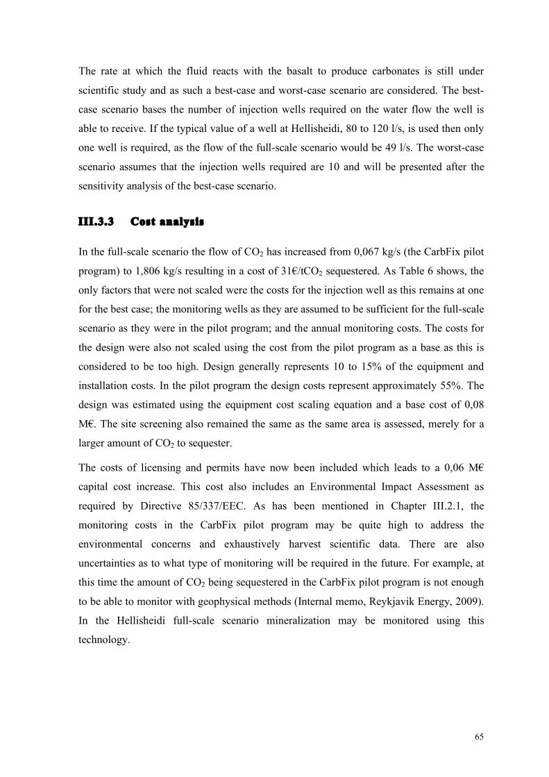
65

The rate at which the fluid reacts with the basalt to produce carbonates is still under

scientific study and as such a best-case and worst-case scenario are considered. The best-

case scenario bases the number of injection wells required on the water flow the well is

able to receive. If the typical value of a well at Hellisheidi, 80 to 120 l/s, is used then only

one well is required, as the flow of the full-scale scenario would be 49 l/s. The worst-case

scenario assumes that the injection wells required are 10 and will be presented after the

sensitivity analysis of the best-case scenario.

III.3.3 Cost analysis

In the full-scale scenario the flow of CO2 has increased from 0,067 kg/s (the CarbFix pilot

program) to 1,806 kg/s resulting in a cost of 31!/tCO2 sequestered. As Table 6 shows, the

only factors that were not scaled were the costs for the injection well as this remains at one

for the best case; the monitoring wells as they are assumed to be sufficient for the full-scale

scenario as they were in the pilot program; and the annual monitoring costs. The costs for

the design were also not scaled using the cost from the pilot program as a base as this is

considered to be too high. Design generally represents 10 to 15% of the equipment and

installation costs. In the pilot program the design costs represent approximately 55%. The

design was estimated using the equipment cost scaling equation and a base cost of 0,08

M!. The site screening also remained the same as the same area is assessed, merely for a

larger amount of CO2 to sequester.

The costs of licensing and permits have now been included which leads to a 0,06 M!

capital cost increase. This cost also includes an Environmental Impact Assessment as

required by Directive 85/337/EEC. As has been mentioned in Chapter III.2.1, the

monitoring costs in the CarbFix pilot program may be quite high to address the

environmental concerns and exhaustively harvest scientific data. There are also

uncertainties as to what type of monitoring will be required in the future. For example, at

this time the amount of CO2 being sequestered in the CarbFix pilot program is not enough

to be able to monitor with geophysical methods (Internal memo, Reykjavik Energy, 2009).

In the Hellisheidi full-scale scenario mineralization may be monitored using this

technology.

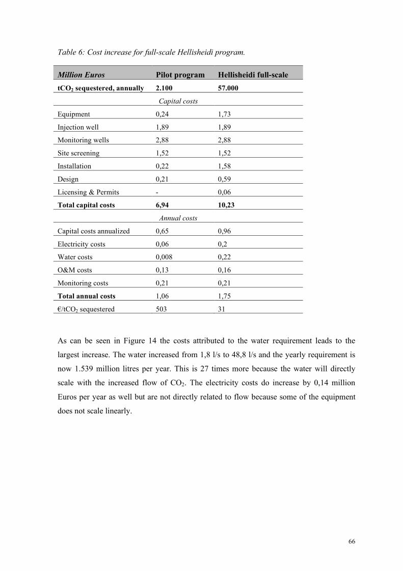
66

Table 6: Cost increase for full-scale Hellisheidi program.

Million Euros Pilot program Hellisheidi full-scale tCO2 sequestered, annually 2.100 57.000

Capital costs

Equipment 0,24 1,73

Injection well 1,89 1,89

Monitoring wells 2,88 2,88

Site screening 1,52 1,52

Installation 0,22 1,58

Design 0,21 0,59

Licensing & Permits - 0,06

Total capital costs 6,94 10,23

Annual costs

Capital costs annualized 0,65 0,96

Electricity costs 0,06 0,2

Water costs 0,008 0,22

O&M costs 0,13 0,16

Monitoring costs 0,21 0,21

Total annual costs 1,06 1,75

!/tCO2 sequestered 503 31

As can be seen in Figure 14 the costs attributed to the water requirement leads to the

largest increase. The water increased from 1,8 l/s to 48,8 l/s and the yearly requirement is

now 1.539 million litres per year. This is 27 times more because the water will directly

scale with the increased flow of CO2. The electricity costs do increase by 0,14 million

Euros per year as well but are not directly related to flow because some of the equipment

does not scale linearly.

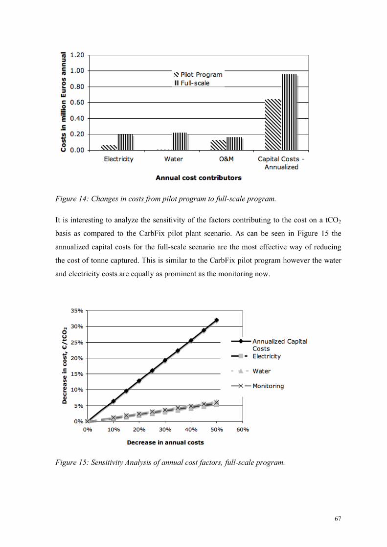
67

Figure 14: Changes in costs from pilot program to full-scale program.

It is interesting to analyze the sensitivity of the factors contributing to the cost on a tCO2

basis as compared to the CarbFix pilot plant scenario. As can be seen in Figure 15 the

annualized capital costs for the full-scale scenario are the most effective way of reducing

the cost of tonne captured. This is similar to the CarbFix pilot program however the water

and electricity costs are equally as prominent as the monitoring now.

Figure 15: Sensitivity Analysis of annual cost factors, full-scale program.

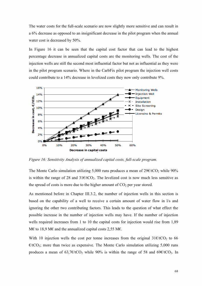
68

The water costs for the full-scale scenario are now slightly more sensitive and can result in

a 6% decrease as opposed to an insignificant decrease in the pilot program when the annual

water cost is decreased by 50%.

In Figure 16 it can be seen that the capital cost factor that can lead to the highest

percentage decrease in annualized capital costs are the monitoring wells. The cost of the

injection wells are still the second most influential factor but not as influential as they were

in the pilot program scenario. Where in the CarbFix pilot program the injection well costs

could contribute to a 14% decrease in levelized costs they now only contribute 9%.

Figure 16: Sensitivity Analysis of annualized capital costs, full-scale program.

The Monte Carlo simulation utilizing 5,000 runs produces a mean of 29!/tCO2 while 90%

is within the range of 28 and 31!/tCO2. The levelized cost is now much less sensitive as

the spread of costs is more due to the higher amount of CO2 per year stored.

As mentioned before in Chapter III.3.2, the number of injection wells in this section is

based on the capability of a well to receive a certain amount of water flow in l/s and

ignoring the other two contributing factors. This leads to the question of what effect the

possible increase in the number of injection wells may have. If the number of injection

wells required increases from 1 to 10 the capital costs for injection would rise from 1,89

M! to 18,9 M! and the annualized capital costs 2,55 M!.

With 10 injection wells the cost per tonne increases from the original 31!/tCO2 to 66

!/tCO2; more than twice as expensive. The Monte Carlo simulation utilizing 5,000 runs

produces a mean of 63,7!/tCO2 while 90% is within the range of 58 and 69!/tCO2. In

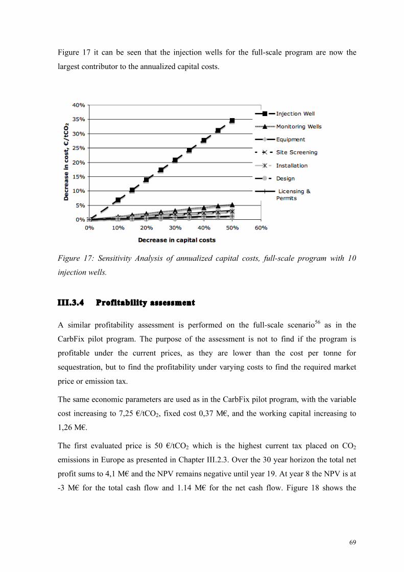
69

Figure 17 it can be seen that the injection wells for the full-scale program are now the

largest contributor to the annualized capital costs.

Figure 17: Sensitivity Analysis of annualized capital costs, full-scale program with 10

injection wells.

III.3.4 Profitability assessment

A similar profitability assessment is performed on the full-scale scenario56 as in the

CarbFix pilot program. The purpose of the assessment is not to find if the program is

profitable under the current prices, as they are lower than the cost per tonne for

sequestration, but to find the profitability under varying costs to find the required market

price or emission tax.

The same economic parameters are used as in the CarbFix pilot program, with the variable

cost increasing to 7,25 !/tCO2, fixed cost 0,37 M!, and the working capital increasing to

1,26 M!.

The first evaluated price is 50 !/tCO2 which is the highest current tax placed on CO2

emissions in Europe as presented in Chapter III.2.3. Over the 30 year horizon the total net

profit sums to 4,1 M! and the NPV remains negative until year 19. At year 8 the NPV is at

-3 M! for the total cash flow and 1.14 M! for the net cash flow. Figure 18 shows the

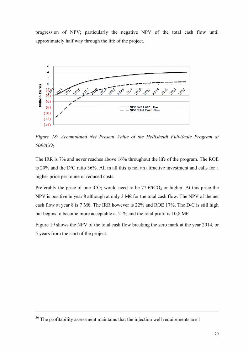
70

progression of NPV; particularly the negative NPV of the total cash flow until

approximately half way through the life of the project.

Figure 18: Accumulated Net Present Value of the Hellisheidi Full-Scale Program at

50!/tCO2.

The IRR is 7% and never reaches above 16% throughout the life of the program. The ROE

is 20% and the D/C ratio 36%. All in all this is not an attractive investment and calls for a

higher price per tonne or reduced costs.

Preferably the price of one tCO2 would need to be 77 !/tCO2 or higher. At this price the

NPV is positive in year 8 although at only 3 M! for the total cash flow. The NPV of the net

cash flow at year 8 is 7 M!. The IRR however is 22% and ROE 17%. The D/C is still high

but begins to become more acceptable at 21% and the total profit is 10,8 M!.

Figure 19 shows the NPV of the total cash flow breaking the zero mark at the year 2014, or

5 years from the start of the project.

56 The profitability assessment maintains that the injection well requirements are 1.

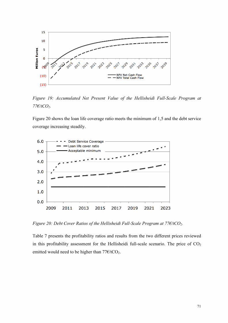
71

Figure 19: Accumulated Net Present Value of the Hellisheidi Full-Scale Program at

77!/tCO2.

Figure 20 shows the loan life coverage ratio meets the minimum of 1,5 and the debt service

coverage increasing steadily.

Figure 20: Debt Cover Ratios of the Hellisheidi Full-Scale Program at 77!/tCO2.

Table 7 presents the profitability ratios and results from the two different prices reviewed

in this profitability assessment for the Hellisheidi full-scale scenario. The price of CO2

emitted would need to be higher than 77!/tCO2.

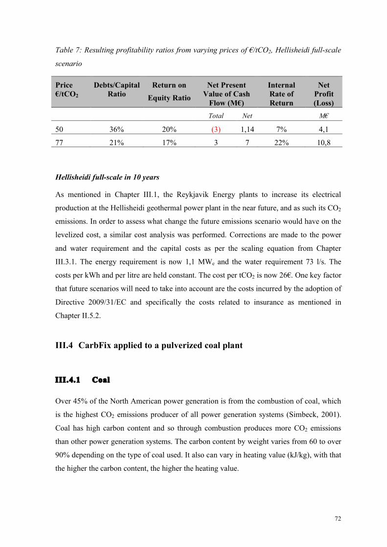
72

Table 7: Resulting profitability ratios from varying prices of !/tCO2, Hellisheidi full-scale

scenario

Price !/tCO2

Debts/Capital Ratio

Return on Equity Ratio

Net Present Value of Cash

Flow (M!)

Internal Rate of Return

Net Profit (Loss)

Total Net M!

50 36% 20% (3) 1,14 7% 4,1

77 21% 17% 3 7 22% 10,8

Hellisheidi full-scale in 10 years

As mentioned in Chapter III.1, the Reykjavik Energy plants to increase its electrical

production at the Hellisheidi geothermal power plant in the near future, and as such its CO2

emissions. In order to assess what change the future emissions scenario would have on the

levelized cost, a similar cost analysis was performed. Corrections are made to the power

and water requirement and the capital costs as per the scaling equation from Chapter

III.3.1. The energy requirement is now 1,1 MWe and the water requirement 73 l/s. The

costs per kWh and per litre are held constant. The cost per tCO2 is now 26!. One key factor

that future scenarios will need to take into account are the costs incurred by the adoption of

Directive 2009/31/EC and specifically the costs related to insurance as mentioned in

Chapter II.5.2.

III.4 CarbFix applied to a pulverized coal plant

III.4.1 Coal

Over 45% of the North American power generation is from the combustion of coal, which

is the highest CO2 emissions producer of all power generation systems (Simbeck, 2001).

Coal has high carbon content and so through combustion produces more CO2 emissions

than other power generation systems. The carbon content by weight varies from 60 to over

90% depending on the type of coal used. It also can vary in heating value (kJ/kg), with that

the higher the carbon content, the higher the heating value.

73

According to the IPCC Special Report on Emission Scenarios (2000) multiple future

energy mix scenarios are analyzed with their corresponding forecasted effect. There are

three specific scenarios, which are of interest specifically due to the characteristics after

2020: A1F1, fossil-intensive, A1T, non-fossil energy sources and A1B, a balance of energy

sources. The fossil-intensive future could result in a 5-degree rise in global temperatures

while even the non-fossil energy source future could still result in a 3-degree rise due to the

higher CO2 concentrations already present prior to 2020.

Coal-fired generating plants are classified according to their steam conditions: sub critical,

supercritical and ultra-supercritical. These different types of cycles have different

efficiencies with the supercritical being the most mature technology and having an

efficiency of 44% and 45% based on the lower heating value, (LHV) (IEA, 2004). Plants in

the USA usually have lower efficiencies when compared to Europe due to the higher

sulphur content in the coal and as such higher flue gas temperatures.

There is also a limit on the efficiency of a coal-fired steam cycle plant, which adheres to

the Carnot efficiency: �= TH – TC/ TH. If the maximum boiler temperature due to the

metallurgical limitations of the steel used is 580°C (Coutsouradis, 1994) and the cooling

water temperature is 20°C than the efficiency limit is 66%57. Once corrections have been

made to the efficiency for internal power requirements and losses it reaches the more

commonly seen figures of approximately 45% (IEA, 2004).

There are discussions in the literature, such as from the IEA, as to whether CCS should be

utilized more in developing nations that have less efficient plants and more emissions. One

argument says that this idea is flawed due to the lower efficiency in these plants. When the

energy requirements due to capture and pressurization are accounted for, the fuel

requirements become higher and as such the emissions increase. However, because the

plant is less efficient the cost for fuel is higher than in comparison to a plant with a more

efficient cycle. Thus the cost of electricity will be higher and the cost of avoidance in

t/CO2 higher (IEA, 2004).

57 �= (580-20)/(580+273)

74

III.4.2 Existing plant and data

The reference plant used in this case is based on work done by Simbeck (2001) and SFA

Pacific, Inc. Simbeck analyzes the costs of a 308 MWe gross pulverized coal plant with

capture and an additional natural gas auxiliary boiler. The information in Table 8

summarizes the plant used as the base reference plant with capture in the CarbFix cost

analysis.

Simbeck, in his analysis58, allows for all but 10% of the original plant capital to be

amortized. This remaining capital is then refinanced with the additional capital for the new

capture equipment and the fixed charged rate set at 15%. The original capital cost

unamortized is 21 M! which added to the new capital gives a total of 269 M!.

Instead of internally consuming the energy penalty for capture, a natural gas boiler is

added and as such additionally the gas fuel costs yearly. There is a flue gas

desulphurization (FGD) system added in order to strip the gas of SO2 and decrease the

occurrences of degradation of amines. Simbeck gives a total cost captured of 18,5!/tCO2.

If the range from the literature, presented in Table 1, is readjusted to Euros the range is 17

to 26 !/tCO2 captured. Thus the cost in the reference plant with capture is within the range,

however on the lower spectrum. This is due to the option to use an older plant with the

remaining capital refinanced.59 The range of increase in capital costs is 34% and the

increase in COE is 0,029!/kWh while the literature gives the range of 0,014 to

0,036!/kWh60 (David, 2000).

58 The analysis by Simbeck is given in USD but has been exchanged to Euros using the exchange rates from Chapter III.2.1. 59 The lower figure can also be a reflection of the lack of inflation correction. 60 Original figures given in USD.

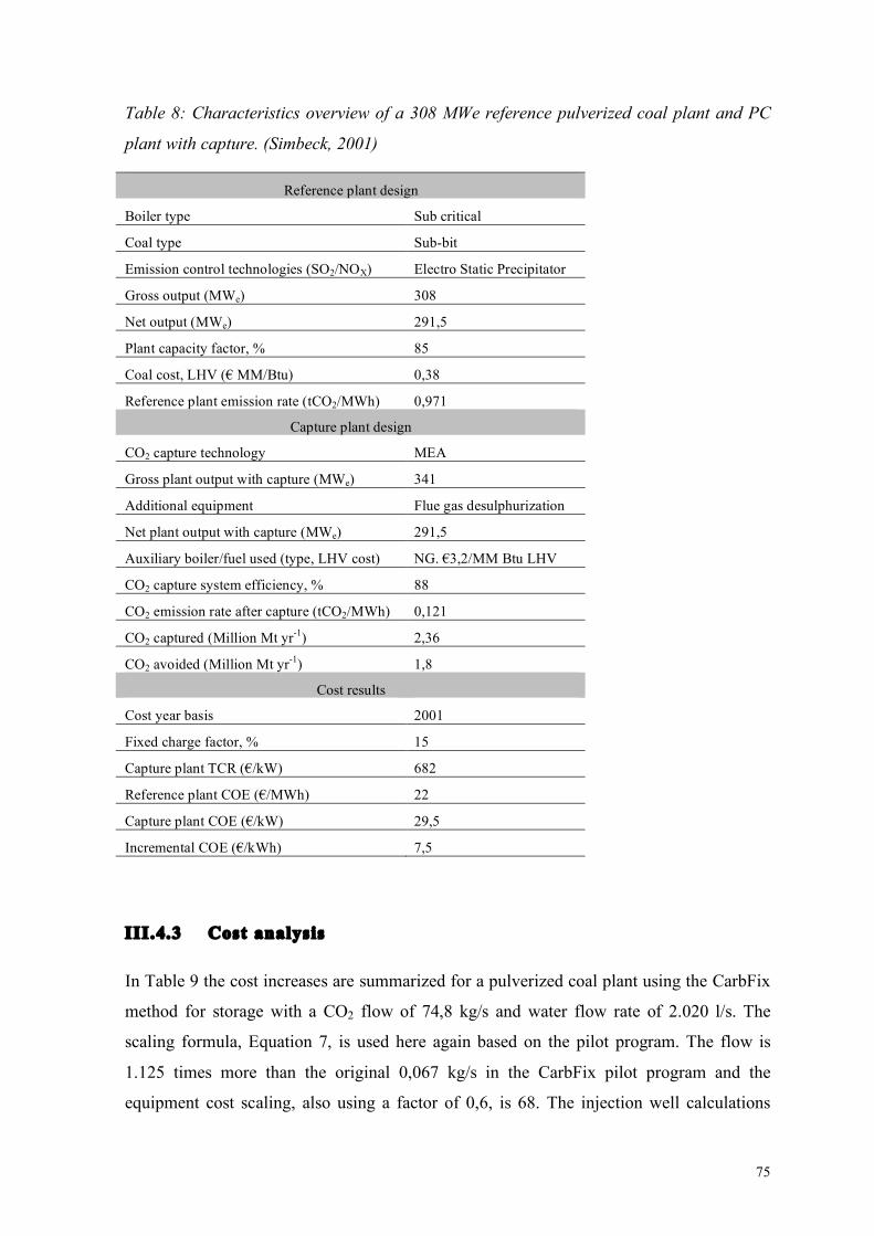
75

Table 8: Characteristics overview of a 308 MWe reference pulverized coal plant and PC

plant with capture. (Simbeck, 2001)

Reference plant design

Boiler type Sub critical

Coal type Sub-bit

Emission control technologies (SO2/NOX) Electro Static Precipitator

Gross output (MWe) 308

Net output (MWe) 291,5

Plant capacity factor, % 85

Coal cost, LHV (! MM/Btu) 0,38

Reference plant emission rate (tCO2/MWh) 0,971

Capture plant design

CO2 capture technology MEA

Gross plant output with capture (MWe) 341

Additional equipment Flue gas desulphurization

Net plant output with capture (MWe) 291,5

Auxiliary boiler/fuel used (type, LHV cost) NG. !3,2/MM Btu LHV

CO2 capture system efficiency, % 88

CO2 emission rate after capture (tCO2/MWh) 0,121

CO2 captured (Million Mt yr-1) 2,36

CO2 avoided (Million Mt yr-1) 1,8

Cost results

Cost year basis 2001

Fixed charge factor, % 15

Capture plant TCR (!/kW) 682

Reference plant COE (!/MWh) 22

Capture plant COE (!/kW) 29,5

Incremental COE (!/kWh) 7,5

III.4.3 Cost analysis

In Table 9 the cost increases are summarized for a pulverized coal plant using the CarbFix

method for storage with a CO2 flow of 74,8 kg/s and water flow rate of 2.020 l/s. The

scaling formula, Equation 7, is used here again based on the pilot program. The flow is

1.125 times more than the original 0,067 kg/s in the CarbFix pilot program and the

equipment cost scaling, also using a factor of 0,6, is 68. The injection well calculations

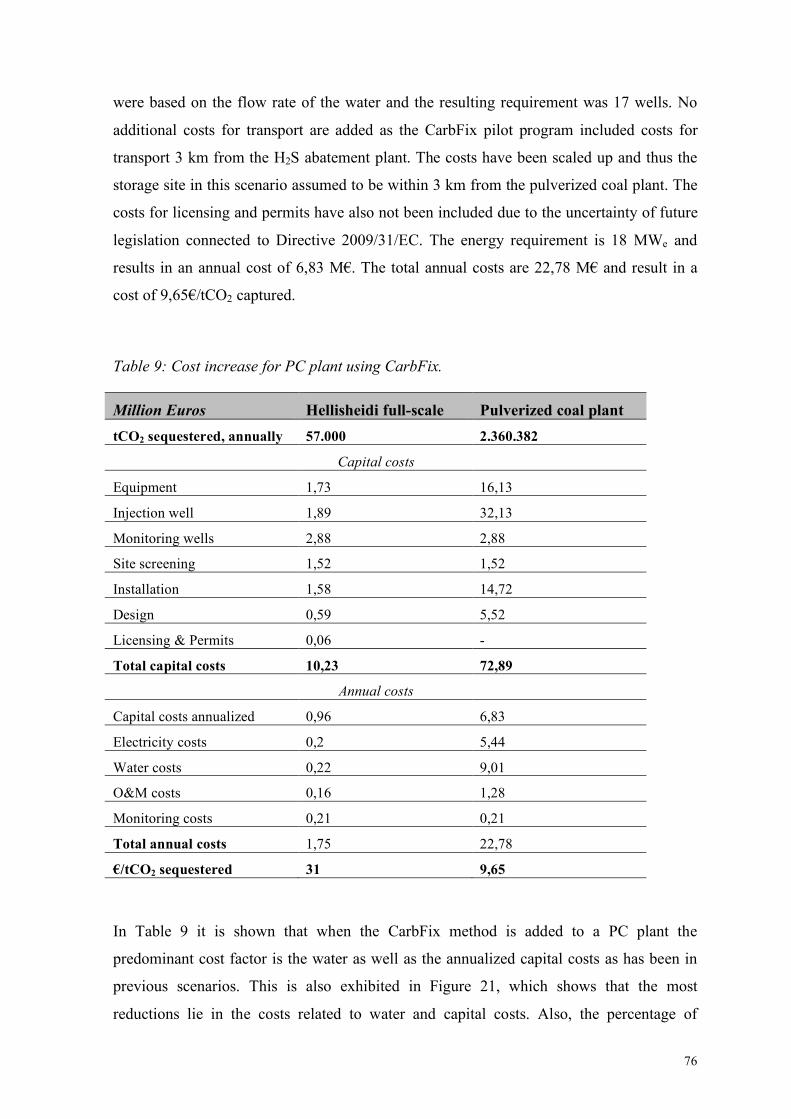
76

were based on the flow rate of the water and the resulting requirement was 17 wells. No

additional costs for transport are added as the CarbFix pilot program included costs for

transport 3 km from the H2S abatement plant. The costs have been scaled up and thus the

storage site in this scenario assumed to be within 3 km from the pulverized coal plant. The

costs for licensing and permits have also not been included due to the uncertainty of future

legislation connected to Directive 2009/31/EC. The energy requirement is 18 MWe and

results in an annual cost of 6,83 M!. The total annual costs are 22,78 M! and result in a

cost of 9,65!/tCO2 captured.

Table 9: Cost increase for PC plant using CarbFix.

Million Euros Hellisheidi full-scale Pulverized coal plant tCO2 sequestered, annually 57.000 2.360.382

Capital costs

Equipment 1,73 16,13

Injection well 1,89 32,13

Monitoring wells 2,88 2,88

Site screening 1,52 1,52

Installation 1,58 14,72

Design 0,59 5,52

Licensing & Permits 0,06 -

Total capital costs 10,23 72,89

Annual costs

Capital costs annualized 0,96 6,83

Electricity costs 0,2 5,44

Water costs 0,22 9,01

O&M costs 0,16 1,28

Monitoring costs 0,21 0,21

Total annual costs 1,75 22,78

!/tCO2 sequestered 31 9,65

In Table 9 it is shown that when the CarbFix method is added to a PC plant the

predominant cost factor is the water as well as the annualized capital costs as has been in

previous scenarios. This is also exhibited in Figure 21, which shows that the most

reductions lie in the costs related to water and capital costs. Also, the percentage of

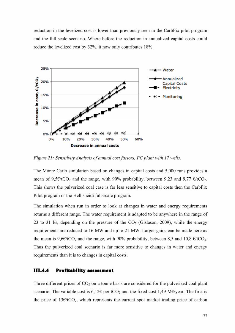
77

reduction in the levelized cost is lower than previously seen in the CarbFix pilot program

and the full-scale scenario. Where before the reduction in annualized capital costs could

reduce the levelized cost by 32%, it now only contributes 18%.

Figure 21: Sensitivity Analysis of annual cost factors, PC plant with 17 wells.

The Monte Carlo simulation based on changes in capital costs and 5,000 runs provides a

mean of 9,5!/tCO2 and the range, with 90% probability, between 9,23 and 9,77 !/tCO2.

This shows the pulverized coal case is far less sensitive to capital costs then the CarbFix

Pilot program or the Hellisheidi full-scale program.

The simulation when run in order to look at changes in water and energy requirements

returns a different range. The water requirement is adapted to be anywhere in the range of

23 to 31 l/s, depending on the pressure of the CO2 (Gislason, 2009), while the energy

requirements are reduced to 16 MW and up to 21 MW. Larger gains can be made here as

the mean is 9,6!/tCO2 and the range, with 90% probability, between 8,5 and 10,8 !/tCO2.

Thus the pulverized coal scenario is far more sensitive to changes in water and energy

requirements than it is to changes in capital costs.

III.4.4 Profitability assessment

Three different prices of CO2 on a tonne basis are considered for the pulverized coal plant

scenario. The variable cost is 6,12! per tCO2 and the fixed cost 1,49 M!/year. The first is

the price of 13!/tCO2, which represents the current spot market trading price of carbon

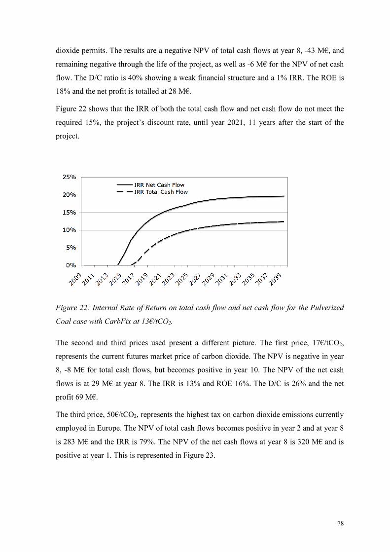
78

dioxide permits. The results are a negative NPV of total cash flows at year 8, -43 M!, and

remaining negative through the life of the project, as well as -6 M! for the NPV of net cash

flow. The D/C ratio is 40% showing a weak financial structure and a 1% IRR. The ROE is

18% and the net profit is totalled at 28 M!.

Figure 22 shows that the IRR of both the total cash flow and net cash flow do not meet the

required 15%, the project’s discount rate, until year 2021, 11 years after the start of the

project.

Figure 22: Internal Rate of Return on total cash flow and net cash flow for the Pulverized

Coal case with CarbFix at 13!/tCO2.

The second and third prices used present a different picture. The first price, 17!/tCO2,

represents the current futures market price of carbon dioxide. The NPV is negative in year

8, -8 M! for total cash flows, but becomes positive in year 10. The NPV of the net cash

flows is at 29 M! at year 8. The IRR is 13% and ROE 16%. The D/C is 26% and the net

profit 69 M!.

The third price, 50!/tCO2, represents the highest tax on carbon dioxide emissions currently

employed in Europe. The NPV of total cash flows becomes positive in year 2 and at year 8

is 283 M! and the IRR is 79%. The NPV of the net cash flows at year 8 is 320 M! and is

positive at year 1. This is represented in Figure 23.

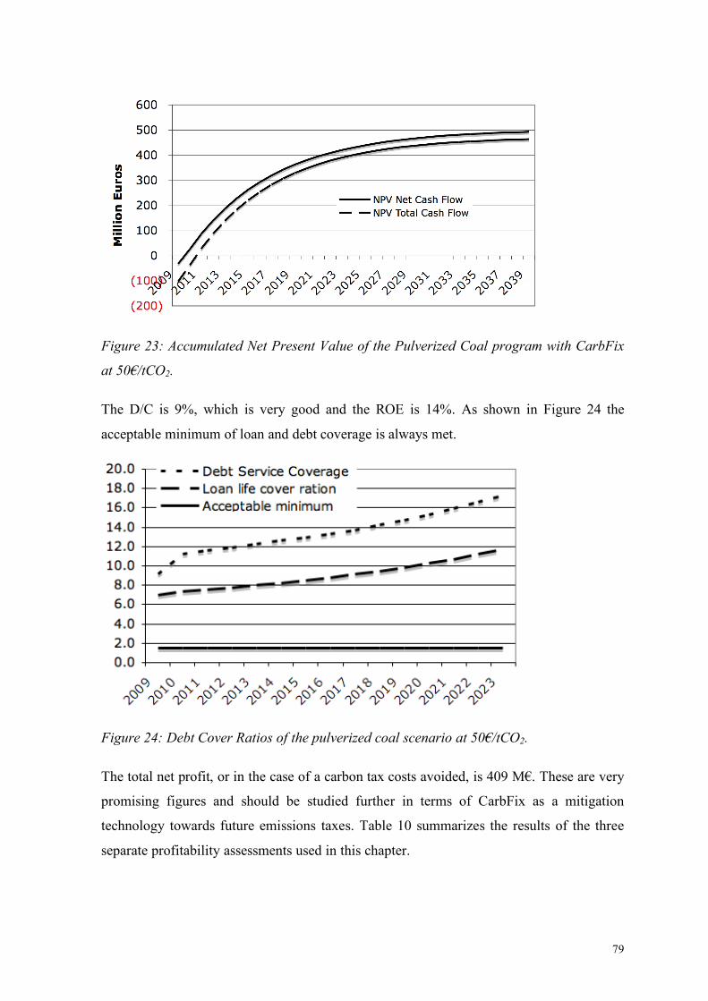
79

Figure 23: Accumulated Net Present Value of the Pulverized Coal program with CarbFix

at 50!/tCO2.

The D/C is 9%, which is very good and the ROE is 14%. As shown in Figure 24 the

acceptable minimum of loan and debt coverage is always met.

Figure 24: Debt Cover Ratios of the pulverized coal scenario at 50!/tCO2.

The total net profit, or in the case of a carbon tax costs avoided, is 409 M!. These are very

promising figures and should be studied further in terms of CarbFix as a mitigation

technology towards future emissions taxes. Table 10 summarizes the results of the three

separate profitability assessments used in this chapter.

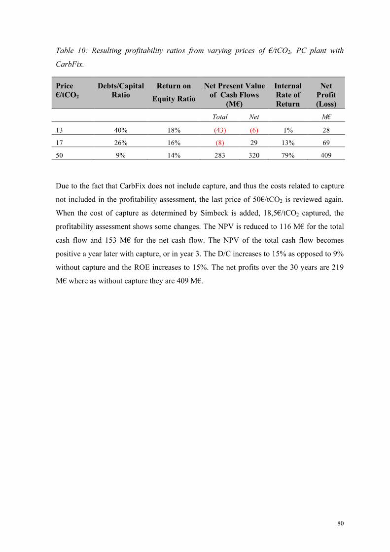
80

Table 10: Resulting profitability ratios from varying prices of !/tCO2, PC plant with

CarbFix.

Price !/tCO2

Debts/Capital Ratio

Return on Equity Ratio

Net Present Value of Cash Flows

(M!)

Internal Rate of Return

Net Profit (Loss)

Total Net M!

13 40% 18% (43) (6) 1% 28

17 26% 16% (8) 29 13% 69

50 9% 14% 283 320 79% 409

Due to the fact that CarbFix does not include capture, and thus the costs related to capture

not included in the profitability assessment, the last price of 50!/tCO2 is reviewed again.

When the cost of capture as determined by Simbeck is added, 18,5!/tCO2 captured, the

profitability assessment shows some changes. The NPV is reduced to 116 M! for the total

cash flow and 153 M! for the net cash flow. The NPV of the total cash flow becomes

positive a year later with capture, or in year 3. The D/C increases to 15% as opposed to 9%

without capture and the ROE increases to 15%. The net profits over the 30 years are 219

M! where as without capture they are 409 M!.

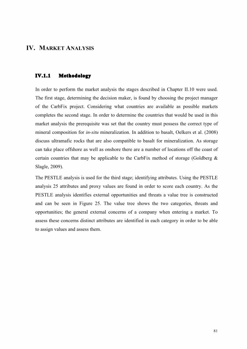
81

IV. MARKET ANALYSIS

IV.1.1 Methodology

In order to perform the market analysis the stages described in Chapter II.10 were used.

The first stage, determining the decision maker, is found by choosing the project manager

of the CarbFix project. Considering what countries are available as possible markets

completes the second stage. In order to determine the countries that would be used in this

market analysis the prerequisite was set that the country must possess the correct type of

mineral composition for in-situ mineralization. In addition to basalt, Oelkers et al. (2008)

discuss ultramafic rocks that are also compatible to basalt for mineralization. As storage

can take place offshore as well as onshore there are a number of locations off the coast of

certain countries that may be applicable to the CarbFix method of storage (Goldberg &

Slagle, 2009).

The PESTLE analysis is used for the third stage; identifying attributes. Using the PESTLE

analysis 25 attributes and proxy values are found in order to score each country. As the

PESTLE analysis identifies external opportunities and threats a value tree is constructed

and can be seen in Figure 25. The value tree shows the two categories, threats and

opportunities; the general external concerns of a company when entering a market. To

assess these concerns distinct attributes are identified in each category in order to be able

to assign values and assess them.

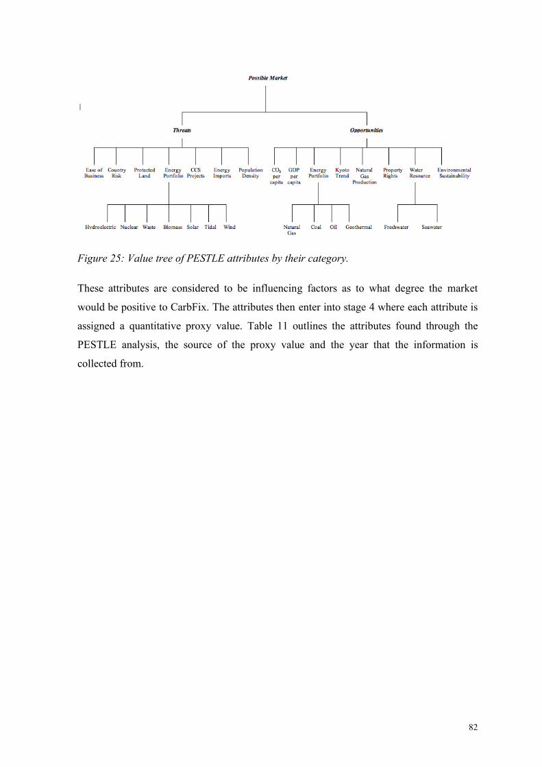
82

Figure 25: Value tree of PESTLE attributes by their category.

These attributes are considered to be influencing factors as to what degree the market

would be positive to CarbFix. The attributes then enter into stage 4 where each attribute is

assigned a quantitative proxy value. Table 11 outlines the attributes found through the

PESTLE analysis, the source of the proxy value and the year that the information is

collected from.

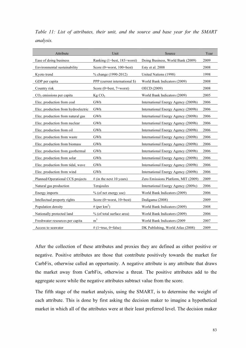
83

Table 11: List of attributes, their unit, and the source and base year for the SMART

analysis.

Attribute Unit Source Year

Ease of doing business Ranking (1=best, 183=worst) Doing Business, World Bank (2009) 2009

Environmental sustainability Score (0=worst, 100=best) Esty et al. 2008 2008

Kyoto trend % change (1990-2012) United Nations (1998) 1998

GDP per capita PPP (current international $) World Bank Indicators (2009) 2008

Country risk Score (0=best, 7=worst) OECD (2009) 2008

CO2 emissions per capita Kg CO2 World Bank Indicators (2009) 2005

Elec. production from coal GWh International Energy Agency (2009b) 2006

Elec. production from hydroelectric GWh International Energy Agency (2009b) 2006

Elec. production from natural gas GWh International Energy Agency (2009b) 2006

Elec. production from nuclear GWh International Energy Agency (2009b) 2006

Elec. production from oil GWh International Energy Agency (2009b) 2006

Elec. production from waste GWh International Energy Agency (2009b) 2006

Elec. production from biomass GWh International Energy Agency (2009b) 2006

Elec. production from geothermal GWh International Energy Agency (2009b) 2006

Elec. production from solar GWh International Energy Agency (2009b) 2006

Elec. production from tidal, wave GWh International Energy Agency (2009b) 2006

Elec. production from wind GWh International Energy Agency (2009b) 2006

Planned/Operational CCS projects # (in the next 10 years) Zero Emissions Platform, MIT (2009) 2009

Natural gas production Terajoules International Energy Agency (2009c) 2006

Energy imports % (of net energy use) World Bank Indicators (2009) 2006

Intellectual property rights Score (0=worst, 10=best) Dedigama (2008) 2009

Population density # (per km2) World Bank Indicators (2009) 2008

Nationally protected land % (of total surface area) World Bank Indicators (2009) 2006

Freshwater resources per capita m3 World Bank Indicators (2009 2007

Access to seawater # (1=true, 0=false) DK Publishing, World Atlas (2008) 2009

After the collection of these attributes and proxies they are defined as either positive or

negative. Positive attributes are those that contribute positively towards the market for

CarbFix, otherwise called an opportunity. A negative attribute is any attribute that draws

the market away from CarbFix, otherwise a threat. The positive attributes add to the

aggregate score while the negative attributes subtract value from the score.

The fifth stage of the market analysis, using the SMART, is to determine the weight of

each attribute. This is done by first asking the decision maker to imagine a hypothetical

market in which all of the attributes were at their least preferred level. The decision maker

84

is then asked if only one attribute could be moved to its most preferred level, which should

that be. The first attribute chosen is freshwater resources per capita and the remaining

attributes are all ranked accordingly. As freshwater resources per capita is the first chosen

attribute it receives a weight of 100. The remaining weights are found by employing swing

weights. Swing weights compare a swing of an attribute from the least preferred level to

most preferred level in comparison to the base weight, or the attribute with a weight of

100. For example the second ranked attribute is electrical production from coal. The

question is then posed, “Consider a swing from a market with no electrical production

from coal to a market where coal is the only source of electrical production with a swing

from a market with no fresh water resources to a country with excess fresh water

resources.” The value given is 95 and as such is the appropriate weight for the attribute

electrical production from coal. Each attribute is swing weighted against the base weight

until all of the attributes have been valued.

As shown in Table 12 the swing weights are summed up to 1.501 and the weights then

normalized. Dividing the attribute weight by the total sum and the result multiplied by 100

normalizes the weights.

85

Table 12: Attribute ranks, swing weights and normalized weights.

Attribute Rank Weight Normalized

Freshwater resources per capita 1 100 6,7

Elec. from coal 2 95 6,3

CO2 emissions per capita 3 90 6,0

Population density 4 89 5,9

Ease of doing business 5 85 5,7

Country risk 6 84 5,6

Elec. from hydroelectric 7 83 5,5

Elec. from nuclear 8 82 5,5

Elec. from waste 9 81 5,4

Elec. from biomass 10 80 5,3

Elec. from solar 11 79 5,3

Elec. from tidal, wave 12 78 5,2

Elec. from wind 13 77 5,1

Energy imports 14 76 5,1

Natural gas production 15 75 5,0

Kyoto trend 16 50 3,3

Planned/Operational CCS projects 17 45 3,0

Environmental sustainability 18 40 2,7

Nationally protected land 19 30 2,0

GDP per capita 20 20 1,3

Elec. from natural gas 21 18 1,2

Elec. from geothermal 22 15 1,0

Elec. from oil 23 14 0,9

Intellectual property rights 24 10 0,7

Access to seawater 25 5 0,3

Total 1.501

A description of the attribute proxy values used in the analysis is given in the next chapter,

IV.1.2. The description discusses both the source of the values used and the effect of the

attribute value on the aggregate score.

86

IV.1.2 Attribute descriptions

Ease of doing business ranking

The Ease of Doing Business score is published in the 2010 Doing Business, a part of the

World Bank publications (2009). It is a measure of the regulations in place for business

activities that take place during the life cycle of a business and the time and actions

required for each activity. A total of 183 countries are compared with a standard case of a

limited liability company of medium size, or 60 employees. The countries are ranked from

1 to 183, with the lower figure being the better score. The Ease of Doing Business score is

only a time and motion indicator score and does not consider economic stability, labour

skills present in the economy, or the strength of the regulating institutions (World Bank,

2010). This proxy value is chosen to represent one of the political factor attributes. It

represents the ease with which business can be done in the prospective market. This is

attribute is listed as a negative because the higher the score, the worse that country is

considered to have an environment that supports ease of doing business.

Environmental sustainability index

The second attribute in the political factors is the environmental sustainability of the

market or the way in which the policies of the country support a sustainable environment.

A proxy of the environmental sustainability index score represents this attribute. This

index considers 21 indicators and which represent 76 data sets. These 21 indicators

represent 5 categories: environmental systems, reducing environmental stresses, reducing

human vulnerability, social and institutional capacity and global stewardship. Each country

receives a score from 0 to 100, with 100 representing the highest value achievable (Esty et

al., 2008). This is a positive attribute as the higher the score the better the country is

promoting environmentally sustainable policies.

Kyoto trend

The attribute “Kyoto Trend” represents both the commitments by Annex I61 countries to

the Kyoto Protocol as well as the trends in emissions shown by non-Annex I countries. The

Kyoto Protocol following the United Nations Framework Convention on Climate Change

61 Annex I countries are defined and listed in the United Nations Framework Convention on Climate Change.

87

(UNFCCC, 1998), is a voluntary commitment by industrialized nations, otherwise known

as Annex I countries, to reduce global greenhouse gases. It is important to note that the

UNFCCC is not a legal binding target but a treaty. The period of the Kyoto Protocol, from

2008 until 2012, sets a reduction target for each country to reduce their emissions of

greenhouse gases by a certain percentage in comparison to their emissions in the base year,

1990 (UNFCCC, 1998). The proxy used for all Annex I countries is the listed commitment

in the Kyoto Protocol unless otherwise stated here.

Article 4 of the Kyoto Protocol allows for those economies that wish to do so to meet their

target reduction together. This is for example done through the European Union member

states that jointly committed to an 8% decrease through the decision by the European

Council in 2004 (Council Decision 280/2004/EC). This joint decision is described as the

EU-15 who reallocated the target reductions amongst themselves in order to reach the

average goal of 8% decrease. Those countries who are part to the EU-15 are here

represented in the Kyoto Trend by the proxy of their commitment to reductions pursuant to

Decision 280/2004/EC.

Because not all countries are party to the Kyoto Protocol and thus have no target, either

because they have not ratified the Protocol through their domestic legislation or because

they are considered to be a non-Annex I country, CO2 emissions data are analyzed and

forecasted. Data is available through the World Bank (2009) in regards to the CO2

emissions total per year from 1990 until 2005. Using this data the years from 2006 until

2012 are forecasted and the percentage increase or decrease from 2012 compared to 1990

levels used as a “trend” value.

The resulting trend figure is either a positive or negative depending on its value. Any

trends that are positive are then reversed to a negative figure, as countries that are

increasing their CO2 emissions are less likely to be considering carbon storage at this

juncture. It is more likely that countries that are exhibiting decreasing trends would have

an open market for storage. Thus, any negative trends are reversed to a positive figure and

contribute to the aggregate score.

GDP per capita

The Gross Domestic Product (GDP) per capita is the sum market value of the final

products and services produced in the boundaries of a country spread over the total of the

population (World Bank, 2007). This indicator gives us a snap shot of the standard of

88

living in a country and is often regarded as a social indicator (van den Bergh, 2009). The

higher the GDP per capita the higher the living conditions in a country although this

indicator does not take into account multiple other factors such as income distribution (van

den Bergh, 2009). This attribute is a positive figure and contributes to the aggregate score.

Country risk

The Country Risk Classification is a rating produced by the Organisation for Economic

Co-operation and Development (OECD). It measures the country’s credit risk or the

possibility of a country defaulting on its external debt62. Generally, the higher the risk

rating of a country is, the higher the risk premium that is placed on interest rates. This

classification was originally done in connection to the Arrangement on Export Credits63 in

order to define the risk premium added to the premium rate (OECD, 2009). The

classification itself does not have to directly relate to a specific company in the country as

an individual company may have a higher credit profile then the country itself. However,

the higher the risk classifications of the country the lower the probability of many

companies in that country being of lower risk. This attribute is negative and subtracts from

the aggregate score as the higher the figure the more risk possibly involved in business

operations in this country.

CO2 emissions per capita

The CO2 emission per capita indicator is collected from the World Bank Indicators. The

World Bank defines carbon dioxide emissions as those resulting from the production for

cement as well as the burning of fossil fuels and the consumption of fuels whether solid,

liquid or gas (World Bank, 2007). Although a high emission per capita would generally be

viewed socially as a negative factor, this attribute is a positive factor. This is due to the fact

that CarbFix would have a more positive entry to markets that have high supplies of CO2

that need to be sequestered.

62 Also known as foreign debt. 63 Trade and Agriculture Directorate of the Organization for Economic Co-operation and Development, Participants to the Arrangement on Officially Supported Export Credits, 5. August, 2009.

89

Electricity production by fuel source

There are 11 attributes that describe the amount of electricity produced by fuel source in

GWh. Some of the attributes are positive while others are negative and this is dependent on

the amount of CO2 produced through their generation. The information on the amount of

GWh produced is collected from the International Energy Agency (2009b).

The positive attributes include electrical production from coal, natural gas, oil and

geothermal. The amount of CO2 emitted per kWh from these sources is 1.160 grams (g),

400 g, 680 g and 40 g respectively (IEA Statistics, 2009). Although geothermal produces a

small amount of CO2 per kWh this is a positive factor because it is the same type of

technology used in the CarbFix pilot program and thus an easily transferred technology.

The negative attributes include electrical production from hydroelectric, nuclear, waste,

biomass, wind, solar (including photovoltaic) and tidal, wave and ocean. These are

negative because capture is performed through pre-combustion, post-combustion and oxy-

combustion. These sources of electrical production do not provide a flue gas source in

which capture could take place.

Planned or operational CCS projects

This attribute takes into account any planned CCS projects or that are already operational.

The value listed is the number of projects that meet the following criteria. The project must

be planned to take place within the next 10 years and must have already have a chosen

storage site. Any project in which the CO2 will be utilized for EOR or EGR was not

included. Projects both with on shore and off shore storage were included. Thus the

number of actual projects may be higher but did not meet the criteria for this evaluation.

The information on the projects was collected from the Zero Emissions Platform database

(2009) as well as from the Massachusetts Institute of Technology (2009).

The value is a negative attribute and subtracts from the aggregate score. This is because

this is considered to be domestic knowledge and thus a competitor in CCS for CarbFix.

Natural gas production

Natural gas contains CO2 that must be stripped away in order for the gas to be sold to users

much like in the Statoil natural gas sales contract (Torp & Gale, 2004). The amount of CO2

that must be separated depends on the contract between the producer and the buyer. A

market where large amounts of natural gas are being produced offers an already available

90

concentrated source of CO2. The costs of capture have already been addressed and the

producer of the natural gas has incurred this cost and should consider it to be a sunk cost.

This attribute then is positive and adds to the aggregate score. This data is compiled from

the IEA statistics on natural gas (IEA, 2009c).

Energy imports as a percentage of net energy use

As CO2 is produced at the source of the immobile emitter, the end-user, or energy buyer,

does not have to consider the CO2 emissions. Countries that import a large part of their

energy have possibly smaller amounts of CO2, or emitter points, available for storage. This

attribute is negative and subtracts from the aggregate score.

Intellectual property rights

The method by which CarbFix performs in-situ mineralization is classified as a service or

purchased knowledge. It is then important that the market in which is entered into has a

strong regulatory system to protect intellectual property rights. The International Property

Rights Index (IPRI) (Dedigama, 2009) was used as a proxy for this attribute. The Index

was designed and modelled to better gauge the effectiveness of domestic regulations in

protecting property rights, both physical and intellectual. The IPRI measures 3 categories;

legal and political environment, physical property rights and intellectual property rights

(IPR). The IPR spans 70 countries in total spanning 95% of the world’s GDP. Countries

are scored from 0 to 10 with the higher figure representing the best possible environment

for protecting intellectual property. This attribute is a positive factor and adds to the

aggregate score.

Population density

The population density was found through the World Bank Indicators database (2009). The

higher the density the more negative the value. This is due to the negative perception the

general public may have towards CCS without further energy literacy of the public. As

CCS would require additional infrastructure and perhaps piping to distant storage sites, the

higher the population density figure may hinder that development. This attribute subtracts

from the aggregate score.

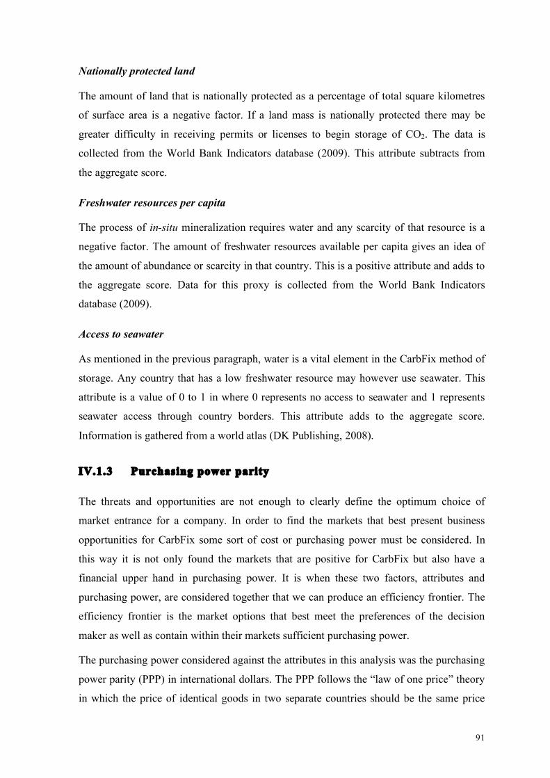
91

Nationally protected land

The amount of land that is nationally protected as a percentage of total square kilometres

of surface area is a negative factor. If a land mass is nationally protected there may be

greater difficulty in receiving permits or licenses to begin storage of CO2. The data is

collected from the World Bank Indicators database (2009). This attribute subtracts from

the aggregate score.

Freshwater resources per capita

The process of in-situ mineralization requires water and any scarcity of that resource is a

negative factor. The amount of freshwater resources available per capita gives an idea of

the amount of abundance or scarcity in that country. This is a positive attribute and adds to

the aggregate score. Data for this proxy is collected from the World Bank Indicators

database (2009).

Access to seawater

As mentioned in the previous paragraph, water is a vital element in the CarbFix method of

storage. Any country that has a low freshwater resource may however use seawater. This

attribute is a value of 0 to 1 in where 0 represents no access to seawater and 1 represents

seawater access through country borders. This attribute adds to the aggregate score.

Information is gathered from a world atlas (DK Publishing, 2008).

IV.1.3 Purchasing power parity

The threats and opportunities are not enough to clearly define the optimum choice of

market entrance for a company. In order to find the markets that best present business

opportunities for CarbFix some sort of cost or purchasing power must be considered. In

this way it is not only found the markets that are positive for CarbFix but also have a

financial upper hand in purchasing power. It is when these two factors, attributes and

purchasing power, are considered together that we can produce an efficiency frontier. The

efficiency frontier is the market options that best meet the preferences of the decision

maker as well as contain within their markets sufficient purchasing power.

The purchasing power considered against the attributes in this analysis was the purchasing

power parity (PPP) in international dollars. The PPP follows the “law of one price” theory

in which the price of identical goods in two separate countries should be the same price

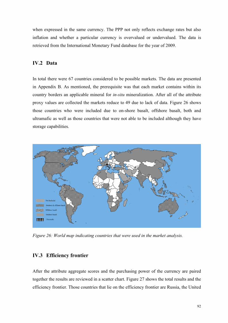
92

when expressed in the same currency. The PPP not only reflects exchange rates but also

inflation and whether a particular currency is overvalued or undervalued. The data is

retrieved from the International Monetary Fund database for the year of 2009.

IV.2 Data

In total there were 67 countries considered to be possible markets. The data are presented

in Appendix B. As mentioned, the prerequisite was that each market contains within its

country borders an applicable mineral for in-situ mineralization. After all of the attribute

proxy values are collected the markets reduce to 49 due to lack of data. Figure 26 shows

those countries who were included due to on-shore basalt, offshore basalt, both and

ultramafic as well as those countries that were not able to be included although they have

storage capabilities.

Figure 26: World map indicating countries that were used in the market analysis.

IV.3 Efficiency frontier

After the attribute aggregate scores and the purchasing power of the currency are paired

together the results are reviewed in a scatter chart. Figure 27 shows the total results and the

efficiency frontier. Those countries that lie on the efficiency frontier are Russia, the United

93

States, Canada, Italy and Germany. Those countries dominate the others in either the

aggregate attribute score or purchasing power. These five countries initially are then the

five that show the most promise as positive markets for CarbFix to enter.

Figure 27: Market analysis efficiency frontier.

It is important to note that a second interview was taken with another applicable decision

maker. The two decision makers differ in roles in the project as well as educational

background. The purpose of the second interview is to note any changes to the efficiency

frontier that may be present. The results show that while there was some difference in the

results in the lower performing countries, ultimately the efficiency frontier presents the

same five countries that should be focused on.

IV.4 Sensitivity analysis

The SMART analysis employs the use of prescriptive weights. In order to better

understand the changes in weights has on the overall outcome a sensitivity analysis is

performed. In this case the weights that are given to the two different categories,

opportunities and threats, will be changed.

The first analysis is to reduce the top three ranked attributes in the category “Threats” to a

weight of zero with all other threats remaining the same. The attributes, population density,

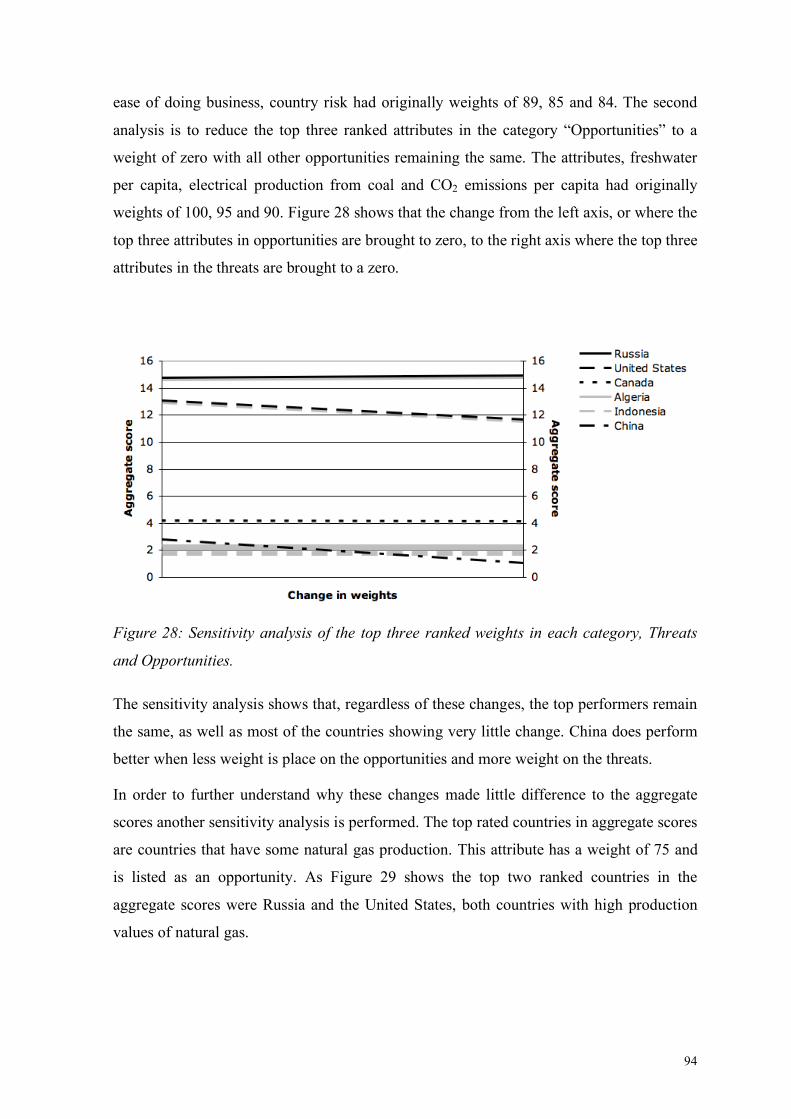
94

ease of doing business, country risk had originally weights of 89, 85 and 84. The second

analysis is to reduce the top three ranked attributes in the category “Opportunities” to a

weight of zero with all other opportunities remaining the same. The attributes, freshwater

per capita, electrical production from coal and CO2 emissions per capita had originally

weights of 100, 95 and 90. Figure 28 shows that the change from the left axis, or where the

top three attributes in opportunities are brought to zero, to the right axis where the top three

attributes in the threats are brought to a zero.

Figure 28: Sensitivity analysis of the top three ranked weights in each category, Threats

and Opportunities.

The sensitivity analysis shows that, regardless of these changes, the top performers remain

the same, as well as most of the countries showing very little change. China does perform

better when less weight is place on the opportunities and more weight on the threats.

In order to further understand why these changes made little difference to the aggregate

scores another sensitivity analysis is performed. The top rated countries in aggregate scores

are countries that have some natural gas production. This attribute has a weight of 75 and

is listed as an opportunity. As Figure 29 shows the top two ranked countries in the

aggregate scores were Russia and the United States, both countries with high production

values of natural gas.

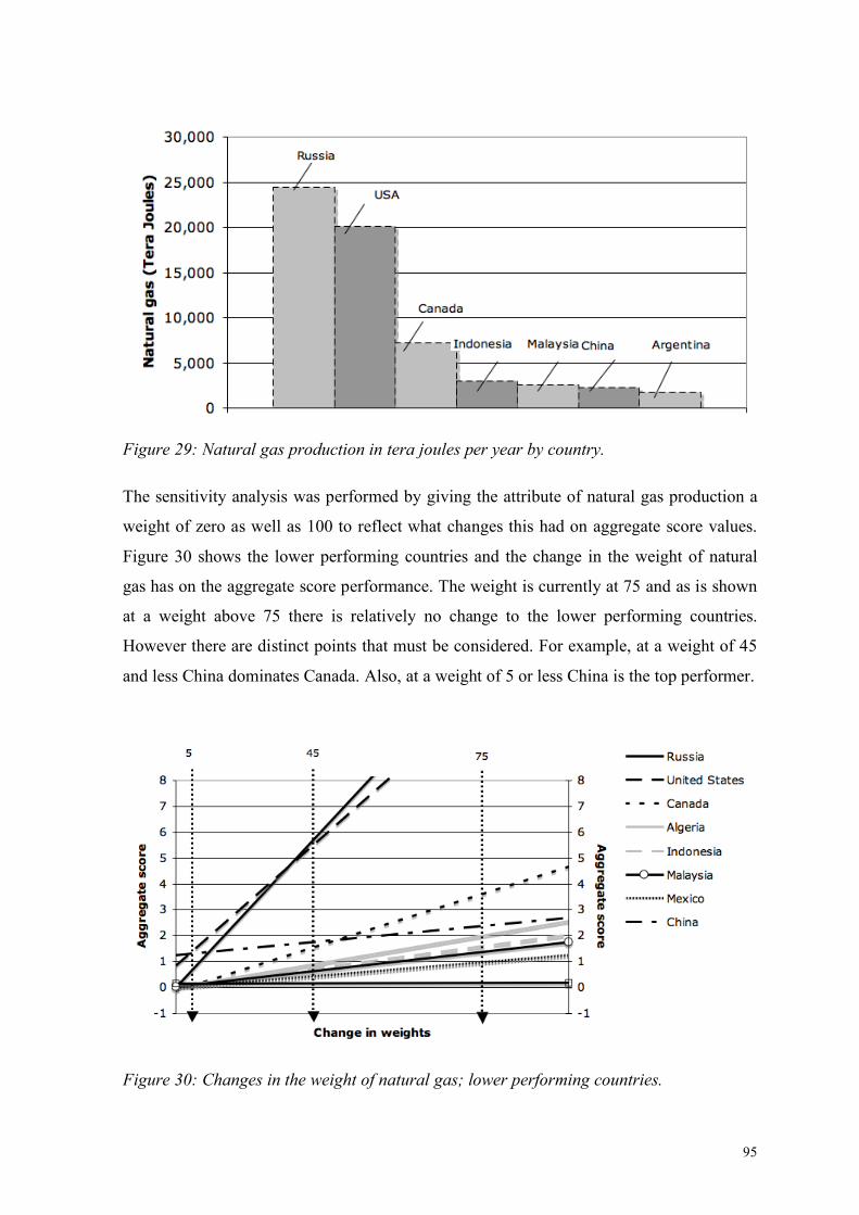
95

Figure 29: Natural gas production in tera joules per year by country.

The sensitivity analysis was performed by giving the attribute of natural gas production a

weight of zero as well as 100 to reflect what changes this had on aggregate score values.

Figure 30 shows the lower performing countries and the change in the weight of natural

gas has on the aggregate score performance. The weight is currently at 75 and as is shown

at a weight above 75 there is relatively no change to the lower performing countries.

However there are distinct points that must be considered. For example, at a weight of 45

and less China dominates Canada. Also, at a weight of 5 or less China is the top performer.

Figure 30: Changes in the weight of natural gas; lower performing countries.

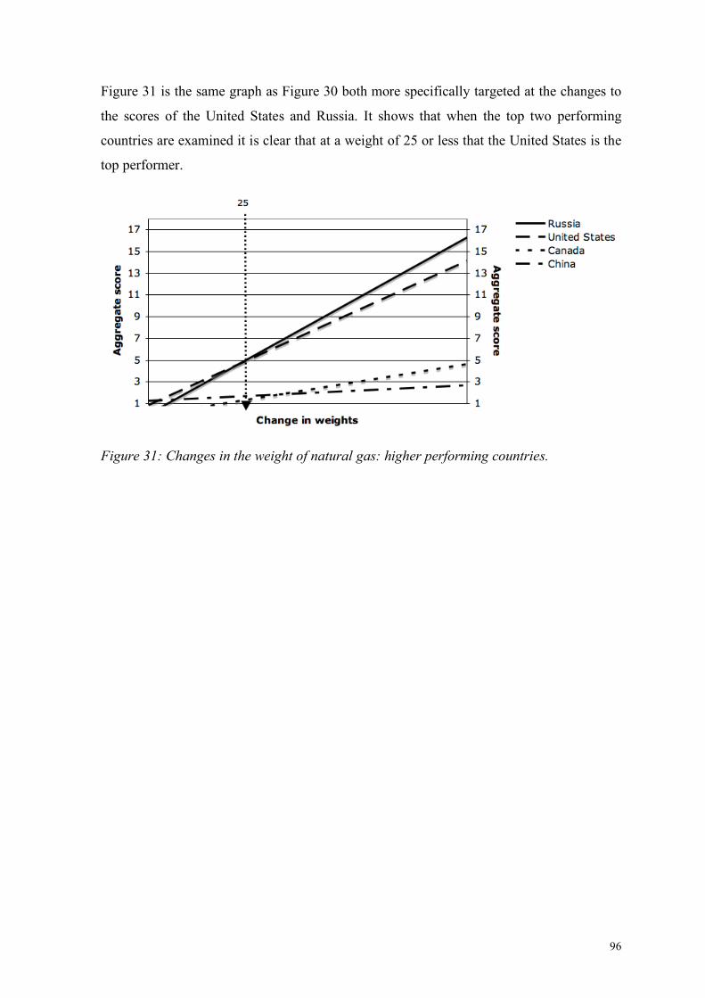
96

Figure 31 is the same graph as Figure 30 both more specifically targeted at the changes to

the scores of the United States and Russia. It shows that when the top two performing

countries are examined it is clear that at a weight of 25 or less that the United States is the

top performer.

Figure 31: Changes in the weight of natural gas: higher performing countries.

97

V. CONCLUSIONS

This paper reviewed the current CarbFix pilot program and its associated costs to find cost

drivers. In order to better understand the changes in cost drivers relative to CO2 flow, two

additional scenarios were considered; the full-scale injection scenario from the Hellisheidi

geothermal power plant, and a capture ready pulverized coal plant. The cost analysis shows

that while the CarbFix pilot program is largely dominated by the capital costs, specifically

monitoring wells, the injection well and site screening, the Hellisheidi full-scale scenario is

dominated by the monitoring wells with all of the other capital costs more evenly spread.

The costs of CO2 captured per tCO2 for these two scenarios are 503! and 31!, respectively.

A sensitivity analysis of both the pilot program and the full-scale scenario shows where the

largest reductions in the cost per tonne can be realized. The pilot program shows relatively

no changes when the water and electricity costs are reduced and this is due to the small

flow of CO2, which the two factors are dependent on. The pilot program can realize the

most reductions in the levelized cost by reducing the capital costs associated to the

monitoring and injection wells. A reduction in these costs of up to 50% can result in a

reduction in the levelized cost in a range from 15 to 23%. The full-scale scenario proves to

be more dependent on the water and electricity requirements, as the flow of CO2 is 27

times more than in the pilot program. A 50% reduction in the water and electrical

requirements could result in a 6% reduction in the levelized cost. Both scenarios, when

applied with a Monte Carlo simulation, show a decreasing sensitivity to capital costs as the

flow increases. The pilot program, with its smaller flow, is the most sensitive providing a

range from 456 to 515!/tCO2. The Hellisheidi scenario shows a much smaller range of 28

to 31!/tCO2.

The pulverized coal plant scenario and its cost analysis is where the greater appeal lies.

The flow is 1.125 times more than in the pilot program and the cost per tonne 9,65!. The

water and electricity costs make up 63% of the total annual costs. The sensitivity analysis

also shows that the water costs are the leading target to reduce the annual costs, providing

up to a 20% reduction in the levelized costs. Even when capture costs are added the total

costs of 28,15!t/CO2 lies within an acceptable range of 18,2 to 35,7!/tCO2 as provided by

the literature. A Monte Carlo simulation also shows that the range of cost per tonne is far

98

less sensitive to changes in capital costs then the changes in the water and electricity

requirements. The range, when the capital costs are tested, is from 9,23 to 9,77!/tCO2

while the range for the water and electricity factors was from 8,5 to 10,8!/tCO2.

These results show that the predominant cost factors are flow dependent and as the flow

increases the CarbFix method of CCS becomes more sensitive to water and electricity

requirements, predominantly the water. When the flow is small the predominant factors are

the capital costs. The number of injection wells is also an important factor and one that

must be studied extensively as the associated capital costs can play a major role. When the

Hellisheidi scenario was increased in regards to injection well requirements, from 1 to 10,

the costs changed drastically. This emphasizes the importance and need for more

geoscientific work concerning injection wells. The cost per tonne increased from 31! to

66!/tCO2, more than twice as expensive. Also, the sensitivity changes as the Monte Carlo

simulation shows that the range is now between 58 and 69!/tCO2. This is an 11-point

difference where the Hellisheidi scenario with one injection well only showed a range of 3

points. The costs analysis also shows that the Hellisheidi full-scale program may become

more economical in the future as the electrical production increases providing more CO2

flow. In 10 years, given that the flow will increase from 60 thousand to 90 thousand tCO2

per year, the cost of the scenario with one injection well decreases from 31!/tCO2 to

26!/tCO2.

The profitability assessment of the three scenarios indicates as to what cost CO2 per tonne

must lie at in order for the scenario, at its current costs, to provide revenue at an acceptable

rate. The CarbFix pilot program provides a price of 1.200!/tCO2 or higher while the

Hellisheidi scenario provides a more reasonable price of 77!/tCO2 or higher. These prices

are dependent on the investor and what the appropriate required return is acceptable, as

well as loan rates and other economic parameter assumptions. However, both scenarios

would find difficulty in competing in a trading market where the current price is

fluctuating around 15!/tCO2.

The pulverized coal plant with capture and CarbFix storage method provides a much more

positive outlook. While a price of 17!/tCO2 could be acceptable, depending on the

investor, a price of 50!/tCO2 would be more reasonable. Even when the capture costs are

included in the profitability assessment the price of 50!/tCO2 still fairs well and offers a

valid investment opportunity. This is comparable to the highest tax currently exhibited in

Europe on energy based CO2 emissions. CarbFix may be better positioned, at its current

99

costs, to work towards a costs avoided scenario where an energy based CO2 tax is

implemented.

The market analysis employs the use of the Simple Multi-Attribute Rating Technique

combined with a PESTLE analysis. The results take into account the external factors, in the

form of opportunities and threats that provide a positive market with low barriers to entry

for CarbFix. The analysis shows that the most efficient markets to enter at this time,

according to the attributes identified and the strength of the market’s currency are Russia,

the United States, Italy and Germany. However, these results may be skewed by the

attribute attached to natural gas production even though it is not a predominant attribute.

When the sensitivity of the top rated threats and opportunities are analyzed there is

relatively no change. When the attribute of natural gas production on its own is tested for

sensitivity there is more change. When this attribute is given a weight of 5 or less China

becomes the top performer while between 5 and 25 the United States outranks the rest.

From the weight of 75 to 100 there is relatively no change with Russia remaining the top

performer and the lower rated countries remaining constant in ranking.

As the SMART analysis is a prescriptive approach it is important that the weights attached

to the attributes are in 100% accordance to the decision maker’s priorities, specifically the

attribute of natural gas production. It is also important that as markets and technologies

change that this sensitivity of the market analysis be reassessed. A Norwegian tax on CO2

in 1991 is one of the main incentives that led to Statoil to store CO2. If more countries

decide to implement a similar tax perhaps the weight of the natural gas attribute should be

increased, as such changing the analysis.

In the future it will be important to work on the major cost factors of the CarbFix method

of storage depending on the flow being assessed. Work should continue in both reducing

capital costs, specifically in the form of monitoring wells, as well as working towards

lower water and energy requirements. The water requirements can be changed according to

the temperature or by using seawater and as such continued research would be needed to

assess what changes this would have on the actual reaction of the basalt and saturated CO2.

The number of required injection wells will also need to be accurately known in order to

bind the capital costs. As the market analysis in this paper only reviewed foreign markets it

would be wise to review the domestic market in terms of potential customers, such as

aluminium smelters. Also, CO2 is a resource and can be utilized in other ways while also

100

providing revenue. Other opportunities should be economically assessed so as to wholly

define all the possible methods of utilization.

This analysis should be reviewed once costs for monitoring are standardized through

legislation both in the international community as well as within the Icelandic legal system.

As Directive 2009/31/EC is adopted into Icelandic legislation and more defining

requirements finalized through the European Council of the European Union additional

factors such as insurance could increase the cost per tonne captured. It is therefore

important for Reykjavik Energy to remain well informed of these changes and

subsequently review this analysis with those changes in mind.

101

REFERENCES

Alfredsson, H.A., Hardarson, B.S., Franzson, H. & Gislason, S.R. (2008, February). CO2 sequestration in basaltic rock at the Hellisheidi site in SW Iceland: Stratigraphy and chemical composition of the rocks at the injection site. Mineralogical Magazine, Vol. 72 (1), pp. 1,5.

Alphen, K. van, Ruijven, J. van, Kasa, S., Hekkert, M., & Turkenburg, W. (2009, September). The performance of the Norwegian carbon dioxide, capture and storage innovation system. Energy Policy 37 (9), pp. 43,55.

American Clean Energy Leadership Act of 2009, S. 1462, 111th Cong., 1st Sess.

Aradottir, E.S.P., Sonnenthal, E., Bjornsson, G., Gunnlaugsson, E. & Jonsson, H. (2009, September 14 - 16). Development of a coupled reactive fluid flow model for mineral CO2 capture in Hellisheidi, Iceland. Paper presented at the 2009 TOUGH Symposium proceedings, Berkeley, CA

Aroonwilas, A., & Veawab, A. (2007). Integration of CO2 capture unit using single- and blended-amines into supercritical coal-fired power plants: Implications for emission and energy management. International Journal of Greenhouse Gas Control (I), pp. 143,150.

Baranzini, A., Goldemberg, J. & Speck, S. (2000). A future for carbon taxes. Ecological Economics (32), pp. 395,412.

Benson, S.M. & Cole, D.R. (2008). CO2 sequestration in deep sedimentary formations. Elements (4), pp. 325,331.

Bloomfield, K.K., Moore, J.N., & Neilson, R.M. (2003, March). Geothermal Energy Reduces Greenhouse Gases. Climate Change Research, pp. 77,79.

Carbon Storage Stewardship Trust Fund Act of 2009, S. 1502, 111th Cong., 1st Sess.

Cheverton, P. (2004). Key marketing skills: strategies, tools, and techniques for marketing success, 2nd Edition. London: Kogan Page Limited.

Cipolli, F., Gambardella, B., Marini, L., Ottonello, G., and Vetuschi Zuccolini, M. (2004, May). Geochemistry of high-pH waters from serpentinites of the Gruppo di Voltri (Genova, Italy) and reaction path modelling of CO2 sequestration in serpentinite aquifers. Applied Geochemistry (19), pp. 787,802.

102

Council Decision 280//2004/EC of 11 February 2004 concerning a mechanism for monitoring community greenhouse gas emissions and for implementing the Kyoto Protocol.

Council Directive (EC) 2003/87/EC of 13 October 2003 on Establishing a Scheme for Greenhouse Gas Emission Allowance Trading within the Community and amending Council Directive 96/61/EC.

Council Directive (EC) 2009/31/EC of 23 April 2009 on the geological storage of carbon dioxide.

Coutsouradis, D. (1994) Materials for Advanced Power Engineering Part II. Netherlands: Kluwer Academic Publishers.

David, J. (2000). Economic evaluation of leading technology options for sequestration of carbon dioxide. Masters Thesis. Massachusetts Institute of Technology, 2000. Retrieved February 15, 2009 from the MIT Libraries.

David, J. & Herzog, H.J. (2001). The cost of carbon capture. Presented at the proceedings of the fifth international conference on greenhouse gas control technologies. Collingwood, Australia.

Dedigama, A.C. (2009). International Property Rights Index (IPRI) 2009 Report. Washington, D.C.: Property Rights Alliance.

Dorling Kindersley Publishing (2008). Essential Atlas of the World. London: Dorling Kindersley Publishing.

Edwards, W. (1971). Social utilities. Engineering Economist, Summer Symposium Series 6, pp. 119,129.

Environmental Protection Agency (2008). Federal requirements under the underground injection control (UIC) program for Carbon Dioxide geological sequestration wells. Federal Register (73), pp. 42492,43451.

Esty, D.C., Levy, M.A., Kim, C.H., de Sherbinin, A., Srebotnjak, T. & Mara, V. (2008). 2008 Environmental Performance Index. New Haven: Yale Center for Environmental Law and Policy.

Goodwin, P. & Wright, G. (2004). Decision analysis for management judgement. 3rd Ed. West Sussex: John Wiley & Sons.

Gislason, S.R., Wolff-Boenisch, D., Stefansson, A., Oelkers, S., Gunnlaugsson, E., Sigurdardottir, H., Sigfusson, B., Broecker, W., Matter, J., Stute, M., Axelsson, G. & Fridriksson, ". (2009). Mineral sequestration of carbon dioxide in basalt: The CarbFix project. International Journal of Greenhouse Gas. Manuscript submitted for publication.

103

Goldberg, D. & Slagle, A. (2009, February). A global assessment of deep-sea basalt sites for carbon sequestration. Energy Procedia (1), pp. 3675,3682.

Ha-Duong, M. & Keith, D.W. (2003, October). CO2 sequestration: the economics of leakage. Clean Technology and Environmental Policy (5), 181-189.

Heddle, G., Herzog, H. & Klett, M. (2003). The economics of CO2 storage. Laboratory for energy and the environment. Cambridge: Massachusetts Institute of Technology.

Hepple, R.P. & Benson, S.M. (2002). Implications of surface seepage on the effectiveness of geologic storage of carbon dioxide as a climate change mitigation strategy. Berkeley: Lawrence Berkeley National Laboratory.

Herzog, H.J. (1999). The economics of CO2 capture. In: Eliasson, B., Riemer, P.W.F., Wokaum, A., editors. Greenhouse gas control technologies. Oxford: Elsevier Science Ltd, pp. 101,106.

Ho, M.T., Allinson, G.W., Wiley, D.E. (2009, February). Factors affecting the cost of capture for Australian lignite coal fired power plants. Energy Procedia (1), pp. 763,770.

Holloway, S. (2005, August). Underground sequestration of carbon dioxide – A viable greenhouse gas mitigation option. Energy (30), pp. 2318,2333.

Huang, B., Hwang, M.J. & Yang, C.W. (2008, August). Causal relationship between energy consumption and GDP growth revisited: A dynamic panel data approach. Ecological Economics (67), pp. 41,54.

IEA (2004). The prospects for CO2 capture and storage. Paris: Organization for Economic Co-Operation & Development/International Energy Agency.

IEA(2007). Legal aspects of storing CO2. Paris: International Energy Agency.

IEA Statistics (2009). CO2 emissions from fuel combustion. Paris: International Energy Agency.

IEA Statistics (2009b). Statistics by country on electricity and heat. Retrieved September 12, 2009, from the International Energy Agency Web site: http://www.iea.org/stats/prodresult.asp?PRODUCT=Electricity/Heat

IEA Statistics (2009c). Statistics by country on natural gas. Retrieved September 12, 2009, from the International Energy Agency Web site: http://www.iea.org/stats/prodresult.asp?PRODUCT=Natural%20Gas

IPCC (2000). Special Report on Emissions Scenarios. Cambridge: Cambridge University Press.

104

IPCC (2005). Underground geological storage. In: Metz, B., Davidson, O., de Coninck, H.C., Loos, M., Meyer, L.A. (Eds) IPCC Special Report on Carbon Dioxide Capture and Storage, prepared by Working Group III of the Intergovernmental Panel on Climate Change. Cambridge: Cambridge University Press.

IMF (2009). World Economic Outlook Database. Retrieved November 25, 2009, from the International Monetary Fund Web site: http://www.imf.org/external/pubs/ft/weo/2009/02/weodata/index.aspx

Kaya, Y. (1990). Impact of carbon dioxide emission control on GNP growth: Interpretation of Proposed Scenarios. Paper presented to the IPCC Energy and Industry Subgroup, Response Strategies Working Group, Paris.

Khalilabad, M.R., Axelsson, G., & Gislason, S.R. (2008, February). Aquifer characterization with tracer test technique; Permanent CO2 sequestration into basalt, SW Iceland. Mineralogical Magazine, (72), pp. 121-125

Marliave, L. de (2009, September). Operational feed back from the first CCS retrofitted power & utility plant. Presented at Carbon Capture & Sequestration Summit, Washington, D.C.

Massachusetts Institute of Technology (2009). Carbon capture and sequestration technologies. Retrieved September 15, 2009, from MIT Carbon Capture Web site: http://sequestration.mit.edu/

Matter, J.M. & Kelemen, P.B. (2009). Permanent storage of carbon dioxide in geological reservoirs by mineral carbonation. Nature Geoscience, Article ngeo683. Retrieved November 1, 2009, from http://www.nature.com/ngeo/journal/vaop/ncurrent/full/ngeo683.html

Matter, J.M., Broecker, W.S., Stute, M., Gislason, S.R., Oelkers, E.H., Stefansson, A., Wolff-Boenisch, D., Gunnlaugsson, E., Axelsson, G. & Bjornsson, G. (2008). Permanent carbon dioxide storage into basalt: The CarbFix pilot project, Iceland. Energy Procedia (1), pp. 3641, 3646.

Mazzotti, M., Pini, R., & Storti, G. (2009, January). Enhanced coal bed methane recovery. Journal of Supercritical Fluids (47), pp. 619,627.

McCollum, D.L. & Ogden, J.M. (2006). Techno-economics models for carbon dioxide compression, transport, and storage. Institute of Transportation Studies, San Francisco: University of California, Davis.

McGee, J., Thomas, H. & Wilson, D. (2005). Strategy analysis & practice. Berkshire: McGraw-Hill Education.

105

McGrail, B.P., Schaef, H.T., Ho, A.M. Chien, Y.J., Dooley, J.J. & Davidson, C.L. (2006). Potential for carbon dioxide sequestration in flood basalts. Journal of Geophysical Research 111, B12201.

Ministerial Council on Mineral and Petroleum Resources (2005). Carbon Dioxide capture and geological storage. Canberra: Australian Regulatory Guiding Principles.

Ministry of the Environment, Norway (1981). Act of 13 March 1981 No. 6 concerning protection against pollution and concerning waste. Oslo, Norway.

Newall, P.S., Clarke, S.J., Haywood, H.M., Scholes, H., Clarke, N.R., King, P.A., & Barley, R.W. (2000). CO2 storage as carbonate minerals. Report PH3/17 for IEA Greenhouse Gas R&D programme, Cornwall: CSMA Consultants Ltd.

Neele, F., Hendriks, C., & Brandsma, R. (2009). Geocapacity: economic feasibility of CCS in networked systems. Presented at the 9th International Conference on Greenhouse Gas Control Technologies, Washington, 16-20 November, 2008.

O’Conner, W.K., Dahlin, D.C., Rush, G.E., Gedermann, S.J., & Penner, L.R. (2007, March). Ex Situ aqueous mineral carbonation. Environmental Science Technology (41), pp. 2587,2593.

OECD (2009). Country risk classifications of the participants to the Arrangement on officially supported export credits. Retrieved September 10, 2009 from the Organization for Economic Co-Operation and Development Web site: http://www.oecd.org/dataoecd/47/29/3782900.pdf

Oelkers, E.H. & Cole, D.R. (2008, October). Carbon dioxide sequestration: A solution to a global problem. Elements (4), pp. 305,310.

Oelkers, E.H., Gislason, S.R. & Matter, J. (2008, October). Mineral Carbonation of CO2. Elements (4), pp. 333,357.

Oishi, O. (2006, June). Mitsubishi CO2 Recovery Technology from Flue Gas. Presented at 9th International CO2 Capture Network, Copenhagen, Denmark.

Point Carbon. Point Carbon EUA OTC assessment – Historical Prices. Retrieved August 20, 2009 from the Point Carbon Web site: http://www.pointcarbon.com/news/historicprices/.

Rubin, E.S., & Rao, A.B. (2002). A technical, economic, and environmental assessment of amine-based CO2 capture technology for power plant greenhouse gas control. Morgantown: U.S. Department of Energy, National Energy Technology Laboratory.

106

Ravagnani, A.T.F.S. G., Ligero, E.L., & Suslick, S.B. (2009, April). CO2 sequestration through enhanced oil recovery in a mature oil field. Journal of Petroleum Science and Engineering (65), pp. 129,138.

Reykjavik Energy (2008). Environmental Report. Retrieved July 15, 2009, from the Reykjavik Energy Web site: http://www.or.is/media/PDF/OR_Umhverfisskyrsla_2008.pdf

Reykjavik Energy (2009). Hellisheidi Power Plant. Retrieved November 2, 2009, from the Reykjavik Energy Web site: http://www.or.is/English/Projects/HellisheidiGeothermalPlant/

Robertson, K., Findsen, J., & Messner, S. (2006). International Carbon Capture and Storage Projects Overcoming Legal Barriers. Morgantown: National Energy Technology Laboratory.

Rubin, E.S., Chen, C. & Rao, A. (2007, September). Cost and performance of fossil fuel power plants with CO2 capture and storage. Energy Policy (35), pp. 4444,4454.

Rubin, E.S. (2008, October). CO2 capture and transport. Elements (4), pp. 311,317.

Sanyal, S. (2005). Cost of geothermal power and factors that affect it. Presented at the proceedings of the World Geothermal Congress, Antalya, Turkey, 24-29 April, 2005.

Sigurdardottir, H. (2008). “CO2 fixation into basalts: Experiment at Hellisheidi geothermal plant.” Reykjavik Energy Graduate School of Sustainable Systems, M-3 Seminar. Reykjavik, Iceland. October 2, 2008.

Sigurdardottir, H. (2009). CarbFix Annual Status Report. Retrieved March 20, 2009, from the Reykjavik Energy Web site: http://www.or.is/English/Projects/CarbFix/AbouttheProject/AnnualStatusReports/

Simbeck, D.R. (2001). CO2 mitigation economics for existing coal-fired power plants. Presented at the First National Conference on Carbon Sequestration, Washington, D.C., May 14-17.

Smith, L.A., Gupta, N., Sass, B.M. & Bubenik, T.A. (2001). Engineering and economic assessment of carbon dioxide sequestration in saline formations. Morgantown: National Energy Technology Laboratory.

Solomon, S., Carpenter, M. & Flach, T.A. (2008, October). Intermediate storage of carbon dioxide in geological formations: A technical perspective. International Journal of Greenhouse Gas Control (2), pp. 502,510.

Torp, T.A. & Gale, J. (2004, July). Demonstrating storage of CO2 in geological reservoirs: The Sleipner and SACS project. Energy (29), pp. 1361,1369.

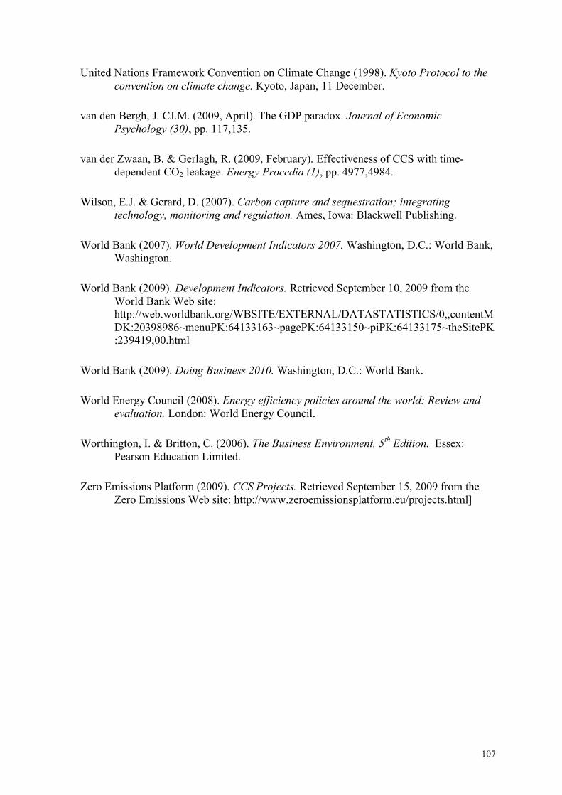
107

United Nations Framework Convention on Climate Change (1998). Kyoto Protocol to the convention on climate change. Kyoto, Japan, 11 December.

van den Bergh, J. CJ.M. (2009, April). The GDP paradox. Journal of Economic Psychology (30), pp. 117,135.

van der Zwaan, B. & Gerlagh, R. (2009, February). Effectiveness of CCS with time-dependent CO2 leakage. Energy Procedia (1), pp. 4977,4984.

Wilson, E.J. & Gerard, D. (2007). Carbon capture and sequestration; integrating technology, monitoring and regulation. Ames, Iowa: Blackwell Publishing.

World Bank (2007). World Development Indicators 2007. Washington, D.C.: World Bank, Washington.

World Bank (2009). Development Indicators. Retrieved September 10, 2009 from the World Bank Web site: http://web.worldbank.org/WBSITE/EXTERNAL/DATASTATISTICS/0,,contentMDK:20398986~menuPK:64133163~pagePK:64133150~piPK:64133175~theSitePK:239419,00.html

World Bank (2009). Doing Business 2010. Washington, D.C.: World Bank.

World Energy Council (2008). Energy efficiency policies around the world: Review and evaluation. London: World Energy Council.

Worthington, I. & Britton, C. (2006). The Business Environment, 5th Edition. Essex: Pearson Education Limited.

Zero Emissions Platform (2009). CCS Projects. Retrieved September 15, 2009 from the Zero Emissions Web site: http://www.zeroemissionsplatform.eu/projects.html]

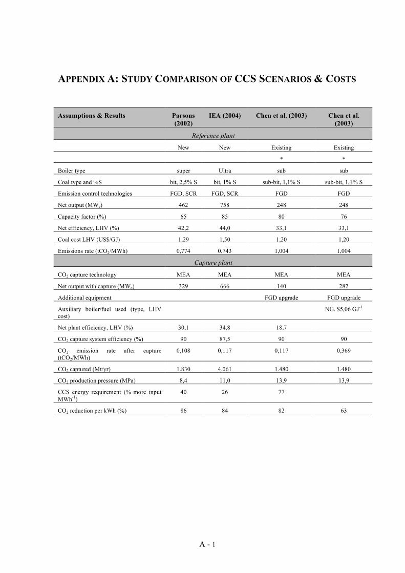
A - 1

APPENDIX A: STUDY COMPARISON OF CCS SCENARIOS & COSTS

Assumptions & Results Parsons (2002)

IEA (2004) Chen et al. (2003) Chen et al. (2003)

Reference plant

New New Existing Existing

* *

Boiler type super Ultra sub sub

Coal type and %S bit, 2,5% S bit, 1% S sub-bit, 1,1% S sub-bit, 1,1% S

Emission control technologies FGD, SCR FGD, SCR FGD FGD

Net output (MWe) 462 758 248 248

Capacity factor (%) 65 85 80 76

Net efficiency, LHV (%) 42,2 44,0 33,1 33,1

Coal cost LHV (US$/GJ) 1,29 1,50 1,20 1,20

Emissions rate (tCO2/MWh) 0,774 0,743 1,004 1,004

Capture plant

CO2 capture technology MEA MEA MEA MEA

Net output with capture (MWe) 329 666 140 282

Additional equipment FGD upgrade FGD upgrade

Auxiliary boiler/fuel used (type, LHV cost)

NG. $5,06 GJ-1

Net plant efficiency, LHV (%) 30,1 34,8 18,7

CO2 capture system efficiency (%) 90 87,5 90 90

CO2 emission rate after capture (tCO2/MWh)

0,108 0,117 0,117 0,369

CO2 captured (Mt/yr) 1.830 4.061 1.480 1.480

CO2 production pressure (MPa) 8,4 11,0 13,9 13,9

CCS energy requirement (% more input MWh-1)

40 26 77

CO2 reduction per kWh (%) 86 84 82 63

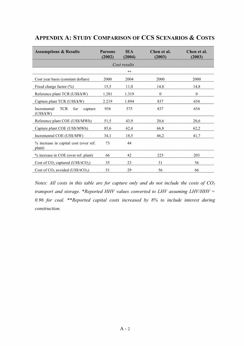
A - 2

APPENDIX A: STUDY COMPARISON OF CCS SCENARIOS & COSTS

Assumptions & Results Parsons (2002)

IEA (2004)

Chen et al. (2003)

Chen et al. (2003)

Cost results **

Cost year basis (constant dollars) 2000 2004 2000 2000

Fixed charge factor (%) 15,5 11,0 14,8 14,8

Reference plant TCR (US$/kW) 1.281 1.319 0 0

Capture plant TCR (US$/kW) 2.219 1.894 837 654

Incremental TCR for capture (US$/kW)

938 575 837 654

Reference plant COE (US$/MWh) 51,5 43,9 20,6 20,6

Capture plant COE (US$/MWh) 85,6 62,4 66,8 62,2

Incremental COE (US$/MW) 34,1 18,5 46,2 41,7

% increase in capital cost (over ref. plant)

73 44

% increase in COE (over ref. plant) 66 42 225 203

Cost of CO2 captured (US$/tCO2) 35 23 31 56

Cost of CO2 avoided (US$/tCO2) 51 29 56 66

Notes: All costs in this table are for capture only and do not include the costs of CO2

transport and storage. *Reported HHV values converted to LHV assuming LHV/HHV =

0.96 for coal. **Reported capital costs increased by 8% to include interest during

construction.

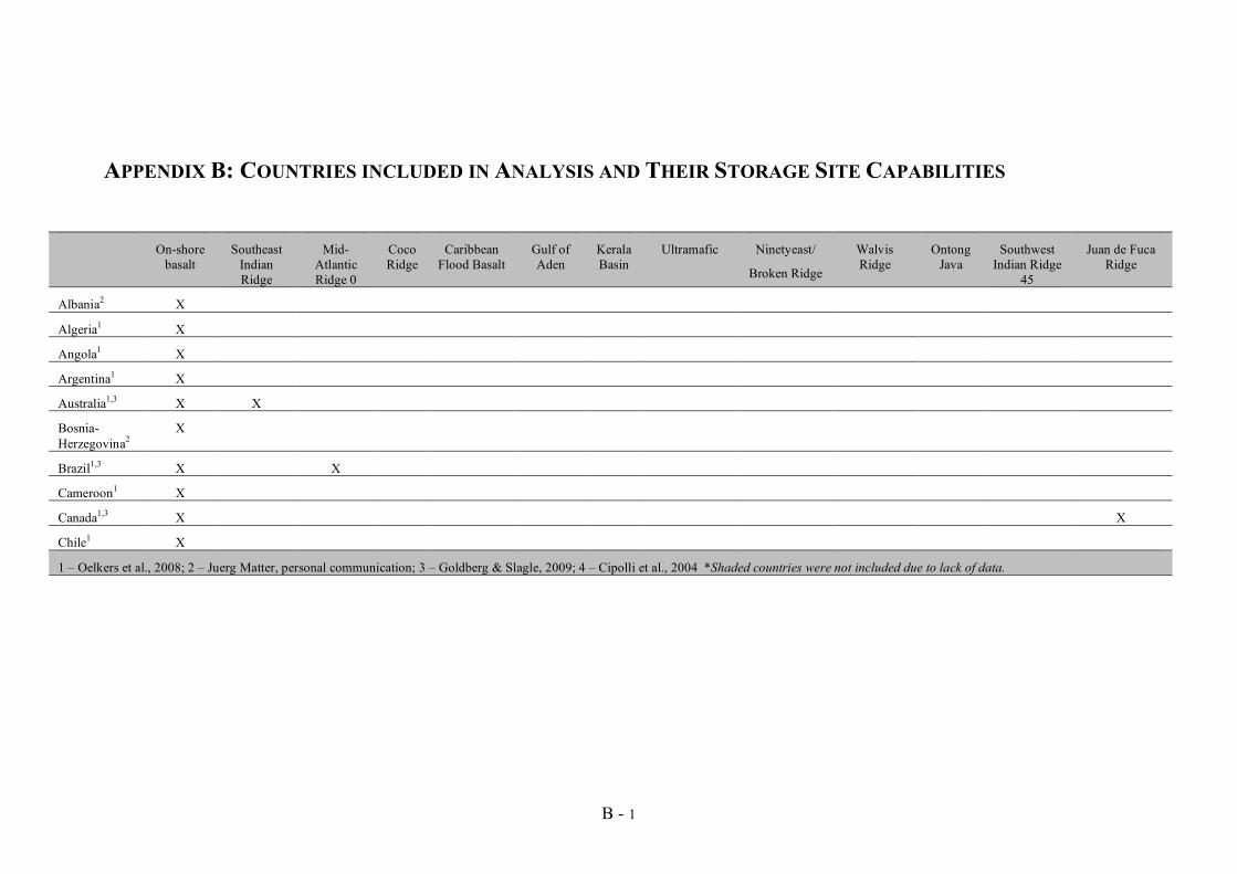
B - 1

APPENDIX B: COUNTRIES INCLUDED IN ANALYSIS AND THEIR STORAGE SITE CAPABILITIES

On-shore basalt

Southeast Indian Ridge

Mid-Atlantic Ridge 0

Coco Ridge

Caribbean Flood Basalt

Gulf of Aden

Kerala Basin

Ultramafic Ninetyeast/

Broken Ridge

Walvis Ridge

Ontong Java

Southwest Indian Ridge

45

Juan de Fuca Ridge

Albania2 X

Algeria1 X

Angola1 X

Argentina1 X

Australia1,3 X X

Bosnia-Herzegovina2

X

Brazil1,3 X X

Cameroon1 X

Canada1,3 X X

Chile1 X

1 – Oelkers et al., 2008; 2 – Juerg Matter, personal communication; 3 – Goldberg & Slagle, 2009; 4 – Cipolli et al., 2004 *Shaded countries were not included due to lack of data.

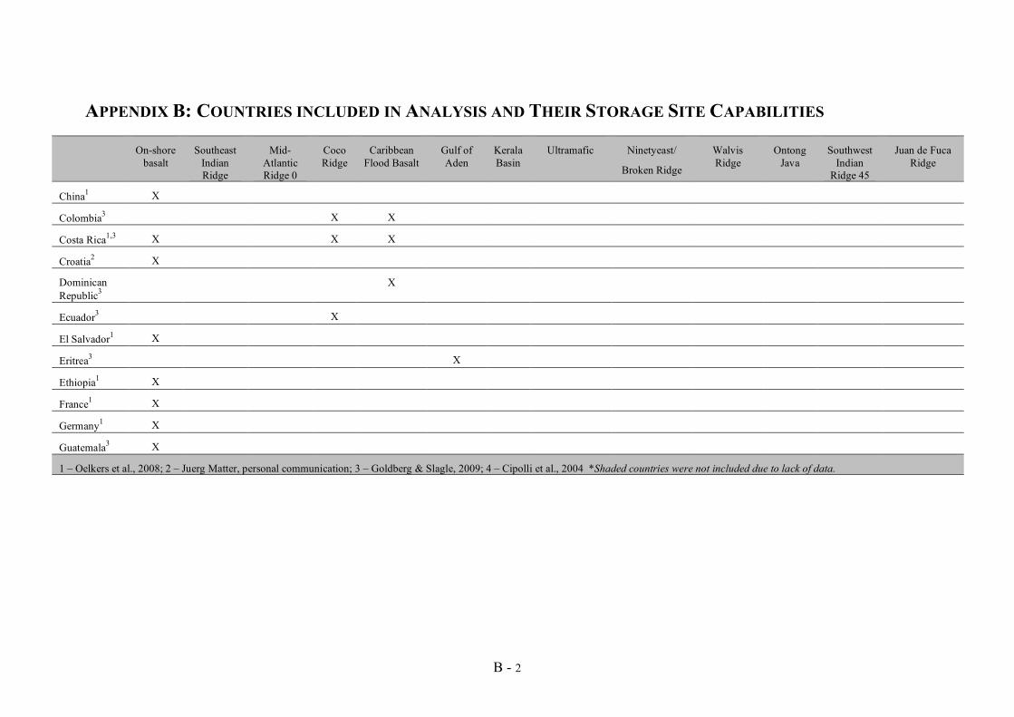
B - 2

APPENDIX B: COUNTRIES INCLUDED IN ANALYSIS AND THEIR STORAGE SITE CAPABILITIES

On-shore basalt

Southeast Indian Ridge

Mid-Atlantic Ridge 0

Coco Ridge

Caribbean Flood Basalt

Gulf of Aden

Kerala Basin

Ultramafic Ninetyeast/

Broken Ridge

Walvis Ridge

Ontong Java

Southwest Indian

Ridge 45

Juan de Fuca Ridge

China1 X

Colombia3 X X

Costa Rica1,3 X X X

Croatia2 X

Dominican Republic3

X

Ecuador3 X

El Salvador1 X

Eritrea3 X

Ethiopia1 X

France1 X

Germany1 X

Guatemala3 X

1 – Oelkers et al., 2008; 2 – Juerg Matter, personal communication; 3 – Goldberg & Slagle, 2009; 4 – Cipolli et al., 2004 *Shaded countries were not included due to lack of data.

B - 3

APPENDIX B: COUNTRIES INCLUDED IN ANALYSIS AND THEIR STORAGE SITE CAPABILITIES

On-shore basalt

Southeast Indian Ridge

Mid-Atlantic Ridge 0

Coco Ridge

Caribbean Flood Basalt

Gulf of Aden

Kerala Basin

Ultramafic Ninetyeast/

Broken Ridge

Walvis Ridge

Ontong Java

Southwest Indian

Ridge 45

Juan de Fuca Ridge

Honduras3 X X

India1,3 X X

Indonesia1 X

Israel1 X

Italy4 X

Japan1 X

Kenya1 X

Malaysia1,3 X X

Mexico1 X

Morocco1 X

Mozambique1 X

Nicaragua1,3 X X X

1 – Oelkers et al., 2008; 2 – Juerg Matter, personal communication; 3 – Goldberg & Slagle, 2009; 4 – Cipolli et al., 2004 *Shaded countries were not included due to lack of data.

B - 4

APPENDIX B: COUNTRIES INCLUDED IN ANALYSIS AND THEIR STORAGE SITE CAPABILITIES

On-shore basalt

Southeast Indian Ridge

Mid-Atlantic Ridge 0

Coco Ridge

Caribbean Flood Basalt

Gulf of Aden

Kerala Basin

Ultramafic Ninetyeast/

Broken Ridge

Walvis Ridge

Ontong Java

Southwest Indian

Ridge 45

Juan de Fuca Ridge

Nigeria1 X

Panama1,3 X X X

Peru3 X

Philippines1 X

Russia1 X

South Africa1,3 X X

Sri Lanka3 X

Tanzania1 X

Turkey1 X

United States1,3 X X

Uruguay1 X

Venezuela1,3 X X

1 – Oelkers et al., 2008; 2 – Juerg Matter, personal communication; 3 – Goldberg & Slagle, 2009; 4 – Cipolli et al., 2004 *Shaded countries were not included due to lack of data.

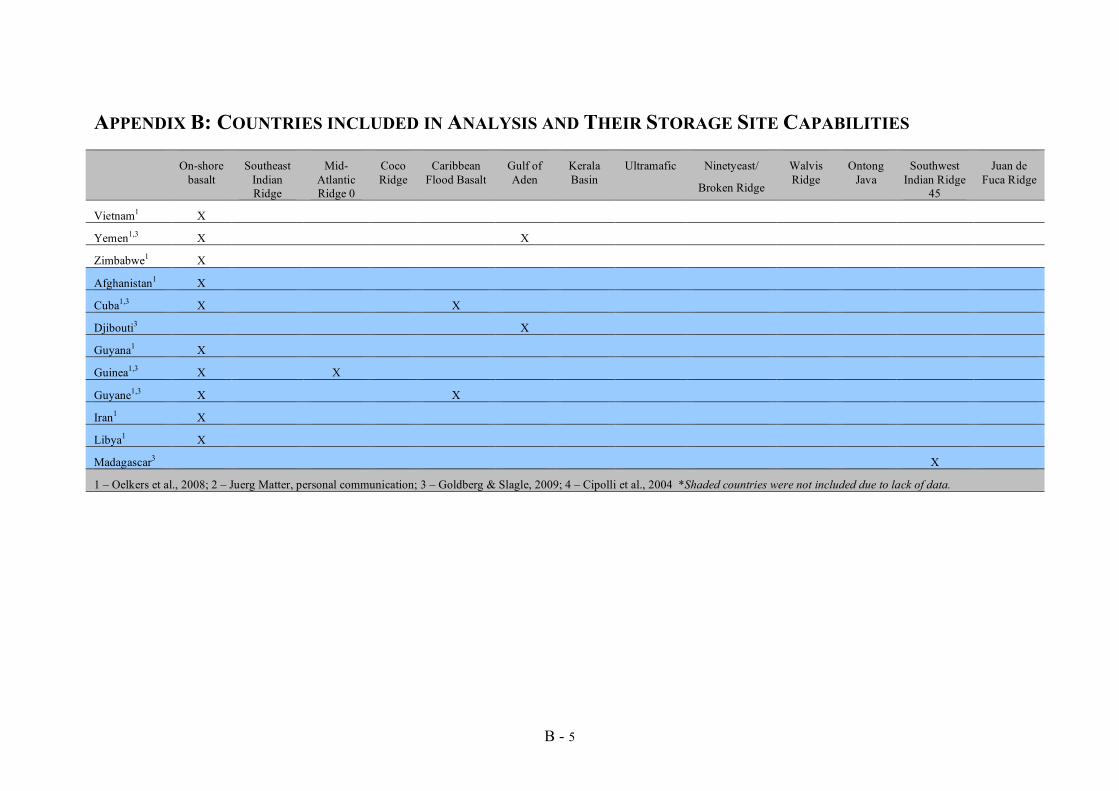
B - 5

APPENDIX B: COUNTRIES INCLUDED IN ANALYSIS AND THEIR STORAGE SITE CAPABILITIES

On-shore basalt

Southeast Indian Ridge

Mid-Atlantic Ridge 0

Coco Ridge

Caribbean Flood Basalt

Gulf of Aden

Kerala Basin

Ultramafic Ninetyeast/

Broken Ridge

Walvis Ridge

Ontong Java

Southwest Indian Ridge

45

Juan de Fuca Ridge

Vietnam1 X

Yemen1,3 X X

Zimbabwe1 X

Afghanistan1 X

Cuba1,3 X X

Djibouti3 X

Guyana1 X

Guinea1,3 X X

Guyane1,3 X X

Iran1 X

Libya1 X

Madagascar3 X

1 – Oelkers et al., 2008; 2 – Juerg Matter, personal communication; 3 – Goldberg & Slagle, 2009; 4 – Cipolli et al., 2004 *Shaded countries were not included due to lack of data.

B - 6

APPENDIX B: COUNTRIES INCLUDED IN ANALYSIS AND THEIR STORAGE SITE CAPABILITIES

On-shore basalt

Southeast Indian Ridge

Mid-Atlantic Ridge 0

Coco Ridge

Caribbean Flood Basalt

Gulf of Aden

Kerala Basin

Ultramafic Ninetyeast/

Broken Ridge

Walvis Ridge

Ontong Java

Southwest Indian Ridge

45

Juan de Fuca Ridge

Montenegro2 X

Namibia1,3 X X

New Caledonia2

X

Oman2,3 X X

Papua New Guinea2,3

X X

Puerto Rico3 X

Saudi Arabia1 X

Somalia3 X

Swaziland1 X

1 – Oelkers et al., 2008; 2 – Juerg Matter, personal communication; 3 – Goldberg & Slagle, 2009; 4 – Cipolli et al., 2004 *Shaded countries were not included due to lack of data.

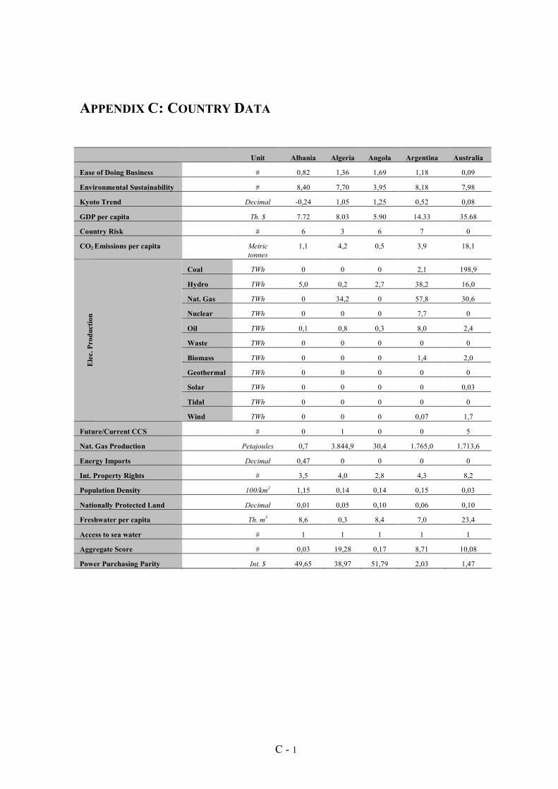
C - 1

APPENDIX C: COUNTRY DATA

Unit Albania Algeria Angola Argentina Australia

Ease of Doing Business # 0,82 1,36 1,69 1,18 0,09

Environmental Sustainability # 8,40 7,70 3,95 8,18 7,98

Kyoto Trend Decimal -0,24 1,05 1,25 0,52 0,08

GDP per capita Th. $ 7.72 8.03 5.90 14.33 35.68

Country Risk # 6 3 6 7 0

CO2 Emissions per capita Metric tonnes

1,1 4,2 0,5 3,9 18,1

Coal TWh 0 0 0 2,1 198,9

Hydro TWh 5,0 0,2 2,7 38,2 16,0

Nat. Gas TWh 0 34,2 0 57,8 30,6

Nuclear TWh 0 0 0 7,7 0

Oil TWh 0,1 0,8 0,3 8,0 2,4

Waste TWh 0 0 0 0 0

Biomass TWh 0 0 0 1,4 2,0

Geothermal TWh 0 0 0 0 0

Solar TWh 0 0 0 0 0,03

Tidal TWh 0 0 0 0 0

Ele

c. P

rodu

ctio

n

Wind TWh 0 0 0 0,07 1,7

Future/Current CCS # 0 1 0 0 5

Nat. Gas Production Petajoules 0,7 3.844,9 30,4 1.765,0 1.713,6

Energy Imports Decimal 0,47 0 0 0 0

Int. Property Rights # 3,5 4,0 2,8 4,3 8,2

Population Density 100/km2 1,15 0,14 0,14 0,15 0,03

Nationally Protected Land Decimal 0,01 0,05 0,10 0,06 0,10

Freshwater per capita Th. m3 8,6 0,3 8,4 7,0 23,4

Access to sea water # 1 1 1 1 1

Aggregate Score # 0,03 19,28 0,17 8,71 10,08

Power Purchasing Parity Int. $ 49,65 38,97 51,79 2,03 1,47

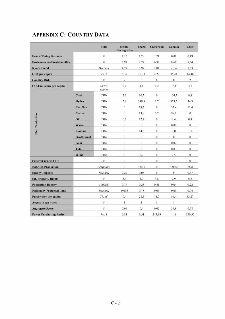
C - 2

APPENDIX C: COUNTRY DATA

Unit Bosnia-Herzegovina

Brazil Cameroon Canada Chile

Ease of Doing Business # 1,16 1,29 1,71 0,08 0,49

Environmental Sustainability # 7,97 8,27 6,38 8,66 8,34

Kyoto Trend Decimal 4,77 0,97 2,01 -0,06 1,33

GDP per capita Th. $ 8,39 10,30 2,22 36,44 14,46

Country Risk # 7 3 6 0 2

CO2 Emissions per capita Metric tonnes

7,0 1,8 0,2 16,6 4,1

Coal TWh 7,3 10,2 0 104,7 9,8

Hydro TWh 5,9 348,8 3,7 355,5 34,3

Nat. Gas TWh 0 18,3 0 33,4 11,4

Nuclear TWh 0 13,8 0,2 98,0 0

Oil TWh 0,2 12,4 0 9,4 0,9

Waste TWh 0 0 0 0,02 0

Biomass TWh 0 14,8 0 9,0 1,1

Geothermal TWh 0 0 0 0 0

Solar TWh 0 0 0 0,02 0

Tidal TWh 0 0 0 0,03 0

Ele

c. P

rodu

ctio

n

Wind TWh 0 0,2 0 2,5 0

Future/Current CCS # 0 0 0 3 0

Nat. Gas Production Petajoules 0 435,1 0 7.206,4 78,8

Energy Imports Decimal 0,27 0,08 0 0 0,67

Int. Property Rights # 3,3 4,7 3,8 7,9 6,5

Population Density 100/km2 0,74 0,23 0,41 0,04 0,22

Nationally Protected Land Decimal 0,005 0,18 0,09 0,01 0,04

Freshwater per capita Th. m3 9,4 28,5 14,7 86,4 53,27

Access to sea water # 1 1 1 1 1

Aggregate Score # 0,09 0,4 0,05 34,9 0,68

Power Purchasing Parity Int. $ 0,81 1,51 243,89 1,18 350,57

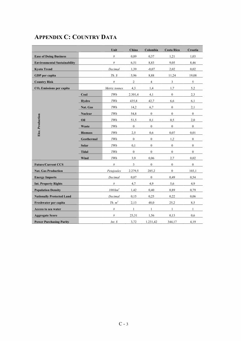
C - 3

APPENDIX C: COUNTRY DATA

Unit China Colombia Costa Rica Croatia

Ease of Doing Business # 0,89 0,37 1,21 1,03

Environmental Sustainability # 6,51 8,83 9,05 8,46

Kyoto Trend Decimal 1,39 -0,07 2,02 0,02

GDP per capita Th. $ 5,96 8,88 11,24 19,08

Country Risk # 2 4 3 5

CO2 Emissions per capita Metric tonnes 4,3 1,4 1,7 5,2

Coal TWh 2.301,4 4,1 0 2,3

Hydro TWh 435,8 42,7 6,6 6,1

Nat. Gas TWh 14,2 6,7 0 2,1

Nuclear TWh 54,8 0 0 0

Oil TWh 51,5 0,1 0,5 2,0

Waste TWh 0 0 0 0

Biomass TWh 2,5 0,6 0,07 0,01

Geothermal TWh 0 0 1,2 0

Solar TWh 0,1 0 0 0

Tidal TWh 0 0 0 0

Ele

c. P

rodu

ctio

n

Wind TWh 3,9 0,06 2,7 0,02

Future/Current CCS # 3 0 0 0

Nat. Gas Production Petajoules 2.279,5 285,2 0 103,1

Energy Imports Decimal 0,07 0 0,49 0,54

Int. Property Rights # 4,7 4,9 5,6 4,9

Population Density 100/km2 1,42 0,40 0,89 0,79

Nationally Protected Land Decimal 0,15 0,25 0,22 0,06

Freshwater per capita Th. m3 2,13 48,0 25,2 8,5

Access to sea water # 1 1 1 1

Aggregate Score # 23,31 1,56 0,13 0,6

Power Purchasing Parity Int. $ 3,72 1.231,42 344,17 4,19

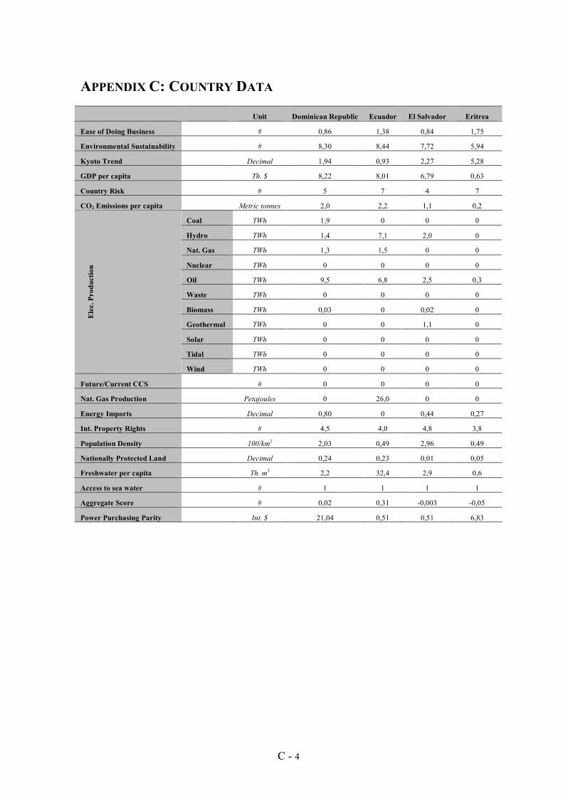
C - 4

APPENDIX C: COUNTRY DATA

Unit Dominican Republic Ecuador El Salvador Eritrea

Ease of Doing Business # 0,86 1,38 0,84 1,75

Environmental Sustainability # 8,30 8,44 7,72 5,94

Kyoto Trend Decimal 1,94 0,93 2,27 5,28

GDP per capita Th. $ 8,22 8,01 6,79 0,63

Country Risk # 5 7 4 7

CO2 Emissions per capita Metric tonnes 2,0 2,2 1,1 0,2

Coal TWh 1,9 0 0 0

Hydro TWh 1,4 7,1 2,0 0

Nat. Gas TWh 1,3 1,5 0 0

Nuclear TWh 0 0 0 0

Oil TWh 9,5 6,8 2,5 0,3

Waste TWh 0 0 0 0

Biomass TWh 0,03 0 0,02 0

Geothermal TWh 0 0 1,1 0

Solar TWh 0 0 0 0

Tidal TWh 0 0 0 0

Ele

c. P

rodu

ctio

n

Wind TWh 0 0 0 0

Future/Current CCS # 0 0 0 0

Nat. Gas Production Petajoules 0 26,0 0 0

Energy Imports Decimal 0,80 0 0,44 0,27

Int. Property Rights # 4,5 4,0 4,8 3,8

Population Density 100/km2 2,03 0,49 2,96 0,49

Nationally Protected Land Decimal 0,24 0,23 0,01 0,05

Freshwater per capita Th. m3 2,2 32,4 2,9 0,6

Access to sea water # 1 1 1 1

Aggregate Score # 0,02 0,31 -0,003 -0,05

Power Purchasing Parity Int. $ 21,04 0,51 0,51 6,83

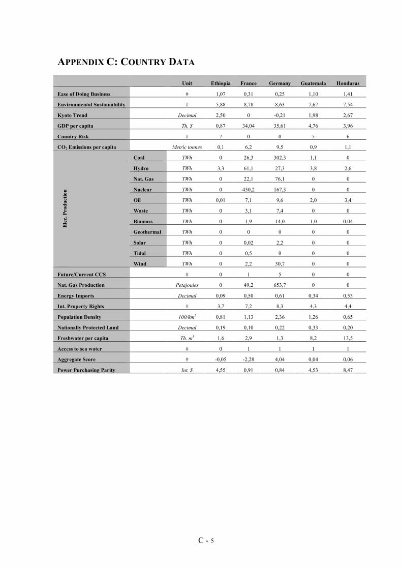
C - 5

APPENDIX C: COUNTRY DATA

Unit Ethiopia France Germany Guatemala Honduras

Ease of Doing Business # 1,07 0,31 0,25 1,10 1,41

Environmental Sustainability # 5,88 8,78 8,63 7,67 7,54

Kyoto Trend Decimal 2,50 0 -0,21 1,98 2,67

GDP per capita Th. $ 0,87 34,04 35,61 4,76 3,96

Country Risk # 7 0 0 5 6

CO2 Emissions per capita Metric tonnes 0,1 6,2 9,5 0,9 1,1

Coal TWh 0 26,3 302,3 1,1 0

Hydro TWh 3,3 61,1 27,3 3,8 2,6

Nat. Gas TWh 0 22,1 76,1 0 0

Nuclear TWh 0 450,2 167,3 0 0

Oil TWh 0,01 7,1 9,6 2,0 3,4

Waste TWh 0 3,1 7,4 0 0

Biomass TWh 0 1,9 14,0 1,0 0,04

Geothermal TWh 0 0 0 0 0

Solar TWh 0 0,02 2,2 0 0

Tidal TWh 0 0,5 0 0 0

Ele

c. P

rodu

ctio

n

Wind TWh 0 2,2 30,7 0 0

Future/Current CCS # 0 1 5 0 0

Nat. Gas Production Petajoules 0 49,2 653,7 0 0

Energy Imports Decimal 0,09 0,50 0,61 0,34 0,53

Int. Property Rights # 3,7 7,2 8,3 4,3 4,4

Population Density 100/km2 0,81 1,13 2,36 1,26 0,65

Nationally Protected Land Decimal 0,19 0,10 0,22 0,33 0,20

Freshwater per capita Th. m3 1,6 2,9 1,3 8,2 13,5

Access to sea water # 0 1 1 1 1

Aggregate Score # -0,05 -2,28 4,04 0,04 0,06

Power Purchasing Parity Int. $ 4,55 0,91 0,84 4,53 8,47

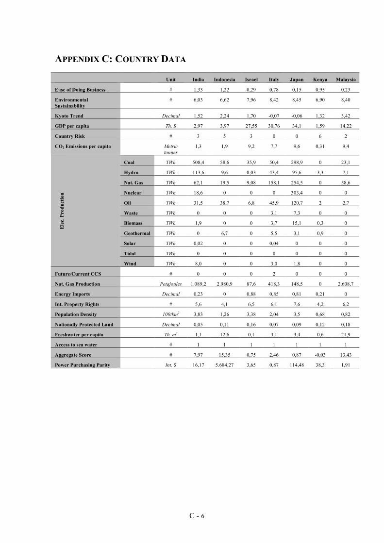
C - 6

APPENDIX C: COUNTRY DATA

Unit India Indonesia Israel Italy Japan Kenya Malaysia

Ease of Doing Business # 1,33 1,22 0,29 0,78 0,15 0,95 0,23

Environmental Sustainability

# 6,03 6,62 7,96 8,42 8,45 6,90 8,40

Kyoto Trend Decimal 1,52 2,24 1,70 -0,07 -0,06 1,32 3,42

GDP per capita Th. $ 2,97 3,97 27,55 30,76 34,1 1,59 14,22

Country Risk # 3 5 3 0 0 6 2

CO2 Emissions per capita Metric tonnes

1,3 1,9 9,2 7,7 9,6 0,31 9,4

Coal TWh 508,4 58,6 35,9 50,4 298,9 0 23,1

Hydro TWh 113,6 9,6 0,03 43,4 95,6 3,3 7,1

Nat. Gas TWh 62,1 19,5 9,08 158,1 254,5 0 58,6

Nuclear TWh 18,6 0 0 0 303,4 0 0

Oil TWh 31,5 38,7 6,8 45,9 120,7 2 2,7

Waste TWh 0 0 0 3,1 7,3 0 0

Biomass TWh 1,9 0 0 3,7 15,1 0,3 0

Geothermal TWh 0 6,7 0 5,5 3,1 0,9 0

Solar TWh 0,02 0 0 0,04 0 0 0

Tidal TWh 0 0 0 0 0 0 0

Ele

c. P

rodu

ctio

n

Wind TWh 8,0 0 0 3,0 1,8 0 0

Future/Current CCS # 0 0 0 2 0 0 0

Nat. Gas Production Petajoules 1.089,2 2.980,9 87,6 418,3 148,5 0 2.608,7

Energy Imports Decimal 0,23 0 0,88 0,85 0,81 0,21 0

Int. Property Rights # 5,6 4,1 6,5 6,1 7,6 4,2 6,2

Population Density 100/km2 3,83 1,26 3,38 2,04 3,5 0,68 0,82

Nationally Protected Land Decimal 0,05 0,11 0,16 0,07 0,09 0,12 0,18

Freshwater per capita Th. m3 1,1 12,6 0,1 3,1 3,4 0,6 21,9

Access to sea water # 1 1 1 1 1 1 1

Aggregate Score # 7,97 15,35 0,75 2,46 0,87 -0,03 13,43

Power Purchasing Parity Int. $ 16,17 5.684,27 3,65 0,87 114,48 38,3 1,91

C - 7

APPENDIX C: COUNTRY DATA

Unit Mexico Morocco Mozambique Nicaragua Nigeria

Ease of Doing Business # 0,51 1,27 1,35 1,17 1,25

Environmental Sustainability

# 7,98 7,21 5,39 7,34 5,62

Kyoto Trend Decimal 0,10 1,21 1,02 0,95 1,76

GDP per capita Th. $ 14,50 4,39 0,86 2,68 2,08

Country Risk # 3 3 6 7 6

CO2 Emissions per capita Metric tonnes 4,1 1,6 0,1 0,7 0,8

Coal TWh 31,7 13,5 0 0 0

Hydro TWh 30,4 1,6 14,7 0,4 7,7

Nat. Gas TWh 113,6 3,0 0,01 0 13,4

Nuclear TWh 10,9 0 0 0 0

Oil TWh 53,8 5,0 0,01 2,1 2,0

Waste TWh 0 0 0 0 0

Biomass TWh 2,5 0 0 0,1 0

Geothermal TWh 6,7 0 0 0,3 0

Solar TWh 0,01 0 0 0 0

Tidal TWh 0 0 0 0 0

Ele

c. P

rodu

ctio

n

Wind TWh 0,06 0,2 0 0 0

Future/Current CCS # 0 0 0 0 0

Nat. Gas Production Petajoules 1.885,6 2,6 103,4 0 1.111,8

Energy Imports Decimal 0 0,95 0 0,39 0

Int. Property Rights # 4,8 5,1 4,2 3,6 3,5

Population Density 100/km2 0,55 0,70 0,28 0,47 1,66

Nationally Protected Land Decimal 0,01 0,01 0,06 0,18 0,06

Freshwater per capita Th. m3 3,9 0,9 4,7 33,9 1,5

Access to sea water # 1 1 1 1 1

Aggregate Score # 9,36 -0,61 0.44 0,21 5,51

Power Purchasing Parity Int. $ 8,06 5,09 13.149,04 7,63 75,42

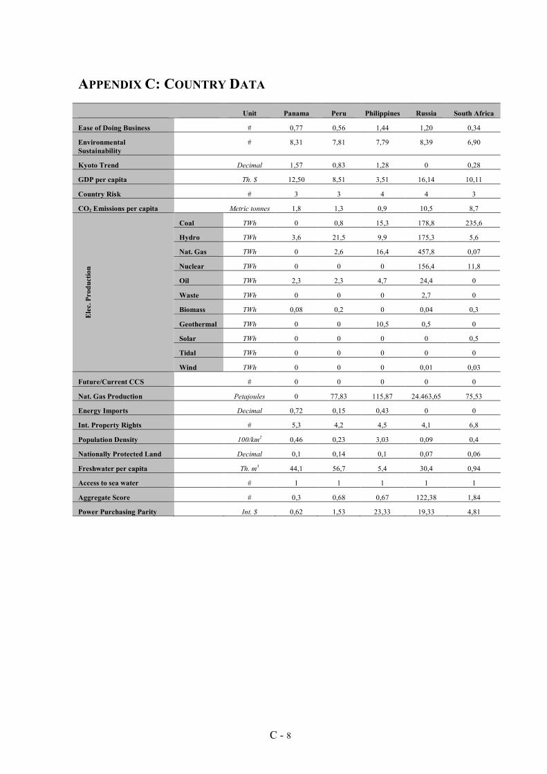
C - 8

APPENDIX C: COUNTRY DATA

Unit Panama Peru Philippines Russia South Africa

Ease of Doing Business # 0,77 0,56 1,44 1,20 0,34

Environmental Sustainability

# 8,31 7,81 7,79 8,39 6,90

Kyoto Trend Decimal 1,57 0,83 1,28 0 0,28

GDP per capita Th. $ 12,50 8,51 3,51 16,14 10,11

Country Risk # 3 3 4 4 3

CO2 Emissions per capita Metric tonnes 1,8 1,3 0,9 10,5 8,7

Coal TWh 0 0,8 15,3 178,8 235,6

Hydro TWh 3,6 21,5 9,9 175,3 5,6

Nat. Gas TWh 0 2,6 16,4 457,8 0,07

Nuclear TWh 0 0 0 156,4 11,8

Oil TWh 2,3 2,3 4,7 24,4 0

Waste TWh 0 0 0 2,7 0

Biomass TWh 0,08 0,2 0 0,04 0,3

Geothermal TWh 0 0 10,5 0,5 0

Solar TWh 0 0 0 0 0,5

Tidal TWh 0 0 0 0 0

Ele

c. P

rodu

ctio

n

Wind TWh 0 0 0 0,01 0,03

Future/Current CCS # 0 0 0 0 0

Nat. Gas Production Petajoules 0 77,83 115,87 24.463,65 75,53

Energy Imports Decimal 0,72 0,15 0,43 0 0

Int. Property Rights # 5,3 4,2 4,5 4,1 6,8

Population Density 100/km2 0,46 0,23 3,03 0,09 0,4

Nationally Protected Land Decimal 0,1 0,14 0,1 0,07 0,06

Freshwater per capita Th. m3 44,1 56,7 5,4 30,4 0,94

Access to sea water # 1 1 1 1 1

Aggregate Score # 0,3 0,68 0,67 122,38 1,84

Power Purchasing Parity Int. $ 0,62 1,53 23,33 19,33 4,81

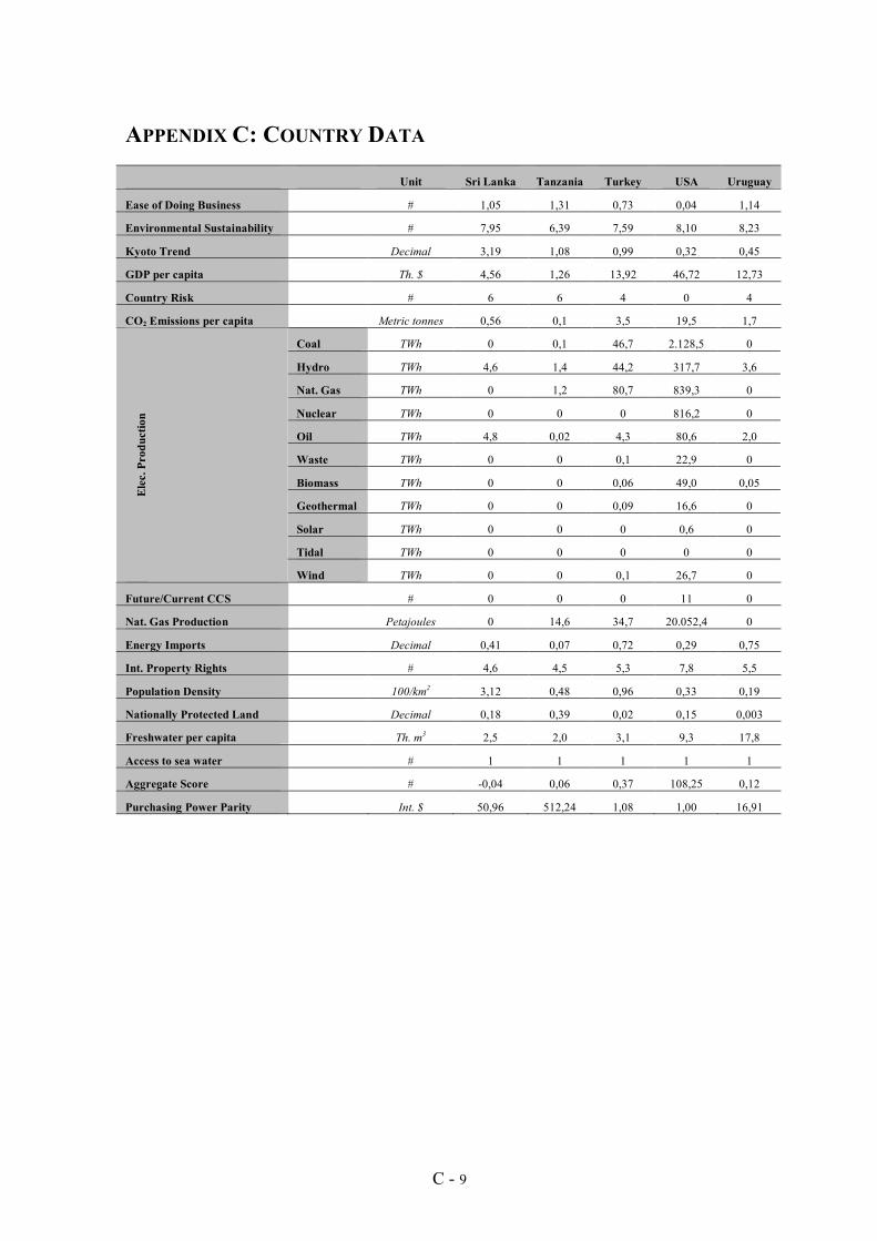
C - 9

APPENDIX C: COUNTRY DATA

Unit Sri Lanka Tanzania Turkey USA Uruguay

Ease of Doing Business # 1,05 1,31 0,73 0,04 1,14

Environmental Sustainability # 7,95 6,39 7,59 8,10 8,23

Kyoto Trend Decimal 3,19 1,08 0,99 0,32 0,45

GDP per capita Th. $ 4,56 1,26 13,92 46,72 12,73

Country Risk # 6 6 4 0 4

CO2 Emissions per capita Metric tonnes 0,56 0,1 3,5 19,5 1,7

Coal TWh 0 0,1 46,7 2.128,5 0

Hydro TWh 4,6 1,4 44,2 317,7 3,6

Nat. Gas TWh 0 1,2 80,7 839,3 0

Nuclear TWh 0 0 0 816,2 0

Oil TWh 4,8 0,02 4,3 80,6 2,0

Waste TWh 0 0 0,1 22,9 0

Biomass TWh 0 0 0,06 49,0 0,05

Geothermal TWh 0 0 0,09 16,6 0

Solar TWh 0 0 0 0,6 0

Tidal TWh 0 0 0 0 0

Ele

c. P

rodu

ctio

n

Wind TWh 0 0 0,1 26,7 0

Future/Current CCS # 0 0 0 11 0

Nat. Gas Production Petajoules 0 14,6 34,7 20.052,4 0

Energy Imports Decimal 0,41 0,07 0,72 0,29 0,75

Int. Property Rights # 4,6 4,5 5,3 7,8 5,5

Population Density 100/km2 3,12 0,48 0,96 0,33 0,19

Nationally Protected Land Decimal 0,18 0,39 0,02 0,15 0,003

Freshwater per capita Th. m3 2,5 2,0 3,1 9,3 17,8

Access to sea water # 1 1 1 1 1

Aggregate Score # -0,04 0,06 0,37 108,25 0,12

Purchasing Power Parity Int. $ 50,96 512,24 1,08 1,00 16,91

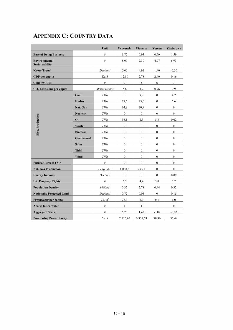
C - 10

APPENDIX C: COUNTRY DATA

Unit Venezuela Vietnam Yemen Zimbabwe

Ease of Doing Business # 1,77 0,93 0,99 1,59

Environmental Sustainability

# 8,00 7,39 4,97 6,93

Kyoto Trend Decimal 0,60 4,91 1,40 -0,50

GDP per capita Th. $ 12,80 2,78 2,40 0,16

Country Risk # 7 5 6 7

CO2 Emissions per capita Metric tonnes 5,6 1,2 0,96 0,9

Coal TWh 0 9,7 0 4,2

Hydro TWh 79,5 23,6 0 5,6

Nat. Gas TWh 14,8 20,9 0 0

Nuclear TWh 0 0 0 0

Oil TWh 16,1 2,3 5,3 0,02

Waste TWh 0 0 0 0

Biomass TWh 0 0 0 0

Geothermal TWh 0 0 0 0

Solar TWh 0 0 0 0

Tidal TWh 0 0 0 0

Ele

c. P

rodu

ctio

n

Wind TWh 0 0 0 0

Future/Current CCS # 0 0 0 0

Nat. Gas Production Petajoules 1.088,6 293,1 0 0

Energy Imports Decimal 0 0 0 0,09

Int. Property Rights # 3,2 4,4 5,0 3,2

Population Density 100/km2 0,32 2,78 0,44 0,32

Nationally Protected Land Decimal 0,72 0,05 0 0,15

Freshwater per capita Th. m3 26,3 4,3 0,1 1,0

Access to sea water # 1 1 1 0

Aggregate Score # 5,23 1,42 -0,02 -0,02

Purchasing Power Parity Int. $ 2.125,63 6.351,69 90,96 35,49

D - 1

APPENDIX D: MAP OF COUNTRIES INCLUDED IN MARKET ANALYSIS