Costs of Production

KW Chapter 8

Costs: Explicit vs. Implicit

• Explicit Costs of Production: Direct payments for resources not owned by a firm (raw materials, wages, energy payments, interest payments).

• Opportunity Cost: (The best alternative to any action).

• Implicit Costs: Opportunity Costs of assets owned by firms– Ex. Owner of barbershop could earn $100 per

hour working as a barber. Implicit cost of the owners time is $100 per hour.

– Opportunity cost of equity capital is return that could have been earned elsewhere.

Short-Run vs. Long Run

• Firms typically have several types of inputs that they can adjust to adjust production.

• Long-run - When firms are able to adjust all of their inputs including physical plant.

• Short-run – When firms are able to adjust only some of their inputs (usually energy, labor, and raw material costs).

Production in the Short-Run

• Given a set of fixed inputs (like plant and capital equipment), a firm can vary other inputs (typically labor) and to vary production.

• Typically, as you add workers, you get more output.

• But, diminishing returns sets in, and the addition of extra workers will generate less and less extra production.

Labor Productivity Function

Output

Labor

Short Run Production Function

OutputMPL

Labor

ΔLabor

ΔOutput

ΔLaborΔOutput

Marginal Product Function

MPL

Labor

Increasing Marginal Product at Low Production Levels

• Up to a point each additional worker adds synergy and adding more workers leads to more and more extra pay-off.

• When a production plant is operating below capacity, adding more workers can generate more output at a relatively constant rate.

Fixed Costs vs. Variable Costs• In short-run, we distinguish between the

costs that are adjustable as production is adjusted (variable costs) and costs that are unchanged regardless of production (fixed costs).– Variable costs (Wages of production workers,

supply and raw materials costs, short-term finance costs)

– Fixed costs (Depreciation costs, Financial costs, wages of non-production workers).

Cost Shares Various 4 Digit Industry

(USA, 1991-1996)

Production NonproductionIndustry Workers Energy Materials Workers Labor IntensityCement 9.02% 17.83% 43.21% 4.23% 34.00%Typesetting 28.17% 0.96% 18.96% 13.07% 51.50%Oil Refinery 1.65% 2.62% 83.80% 1.07% 20.09%Automobiles 5.41% 0.37% 71.97% 1.06% 23.38%Furniture 18.03% 1.62% 47.86% 5.56% 46.68%Mens Clothes 20.20% 1.23% 40.08% 7.67% 47.49%

NBER Productivity Database

Types of Costs

• Total Fixed Costs – Invariant to the number of goods produced (in the short-run)

• Total Variable Costs- Increasing in the number of goods produced.

• Total Costs: Fixed Costs + Variable Costs

Bakery: Wages $10 per Worker, $5 Wheat per Loaf

Output Fixed Workers Bakers Wheat Variable Total(Loaves) Costs Wages Costs Costs

0.00 1000 0 0 0.00 0.00 1000.00

10.00 1000 10 100 50.00 150.00 1150.00

20.00 1000 40 400 100.00 500.00 1500.00

30.00 1000 90 900 150.00 1050.00 2050.00

40.00 1000 160 1600 200.00 1800.00 2800.00

50.00 1000 250 2500 250.00 2750.00 3750.00

60.00 1000 360 3600 300.00 3900.00 4900.00

Total Variable Costs are increasing at an accelerating rate.

Reason: Diminishing returns to variable inputs.

0

1000

2000

3000

4000

5000

6000

0.00 10.00 20.00 30.00 40.00 50.00 60.00

Output

Fixed Costs Variable Costs Total Costs

Costs: Average vs. Marginal

• Total Costs are the sum of all relevant costs for a firm.

• Average Costs: Costs per unit of output.

• Marginal Cost: Extra Cost per Extra Unit of Output.

Average and Marginal CostsAverage Fixed Costs decreases as production increases

AVC, ATC, MC all increase as diminishing returns kick in

MC equals AVC and ATC when each of the latter are at their minimum level. -15

5

25

45

65

85

105

125

0.00

5.00

10.00

15.00

20.00

25.00

30.00

35.00

40.00

45.00

50.00

55.00

60.00

Output

Average Fixed Costs Average Variable Costs

Average Total Costs Average Marginal Costs

Cost SchedulesOutput Average Average Average

Total Fixed Variable Total Marginal(Loaves) Costs Costs Costs Costs Costs

0.00 1000.0015.00

10.00 1150.00 100 15 11535.00

20.00 1500.00 50 25 7555.00

30.00 2050.00 33.33333 35 6875.00

40.00 2800.00 25 45 7095.00

50.00 3750.00 20 55 75115.00

60.00 4900.00 16.66667 65 82

Costs in the Long Run

• In the short-run, the size of a firms physical plant is a fixed factor.

• Over-time, the plant size can adjust.

• In the bakery example, extra ovens can be added.

Minimizing Costs in the Long Run

• Consider average total cost schedules at different numbers of ovens.

• Each oven will have a production level that generates the minimum average total cost.

• To minimize average costs in the long-run, choose the number of ovens which will have the lowest, minimum average total cost.

Average Total Cost Schedules at Different Scales of Production

48

68

88

108

128

148

168

188

208

2281

0

20

30

40

50

60

70

80

90

10

0

11

0

12

0Output

1 Oven

2 Ovens

3 Ovens

4 Ovens

5 Ovens

6 Ovens

7 Ovens

8 Ovens

Minimum of the different cost Schedules

48

68

88

108

128

148

168

188

208

2281

0

20

30

40

50

60

70

80

90

10

0

11

0

12

0Output

1 Oven

2 Ovens

3 Ovens

4 Ovens

5 Ovens

6 Ovens

7 Ovens

8 Ovens

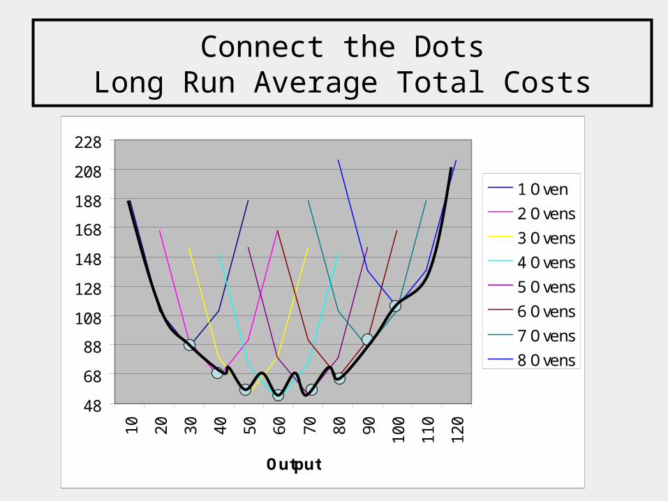
Connect the DotsLong Run Average Total Costs

48

68

88

108

128

148

168

188

208

2281

0

20

30

40

50

60

70

80

90

10

0

11

0

12

0Output

1 Oven

2 Ovens

3 Ovens

4 Ovens

5 Ovens

6 Ovens

7 Ovens

8 Ovens

If we adjust capital scale continuously, the collection of minimum points is the

Long Run Average Total cost cuve

LR ATC

Short-run ATC

Economies of Scale• When firms are able to adjust all of their inputs,

they can choose a size that will minimize costs. • If a firm is able to achieve some economies of

scale, increasing size will reduce the average total cost.

• Sources of Economies of Scale– Production requires major expenditure on items needed

to produce even zero products• Ex. Software, pharmaceuticals

– Production requires many specific steps which can be most efficiently done through specialization

• Ex. Airplanes, automobiles

Long Run ATC increasing returns to scale.

Output

Costs

LR ATC

Economies of Scale

Returns to Scale

• Scale Economies is not always likely to characterize production.

• If each production unit can act autonomously with identical costs then we may experience constant returns to scale.

• Firms at some point experience diseconomies of scale or increasing long run average total costs.

• Sources of diseconomies of scale– Limits of managerial invention. – Limits of some other fixed resource.

Long Run ATC decreasing returns to scale.

Output

Costs

LR ATC

Constant Returns Scale

Diseconomies

Overall Cost Function

LR ATC

Minimum Efficient Scale

MES and Market Structure

• If MES is relatively large in comparison with the market demand:

$

Q

D

LRAC

The market is most efficiently served by a single firm---natural monopoly!

MES and Market Structure

• If MES is relatively small in comparison with market demand:

$

Q

Many “small” firms in the market.

Typical Scale varies across sectors in USA

Sales per Establishment

0

5000

10000

15000

20000

25000

Mining Utilities Construction Manufacturing Retail trade Professional,scientific, &

technicalservices

2002 Census of Manufactures

Learning OutcomesStudents should be able to • Define and calculate various types of economic costs.

– Explicit, implicit, fixed, variable, total, average, marginal, economic, accounting.

• Describe the shape of various relevant cost curves– Average Total (in LR and SR), Average Fixed,

Marginal Costs• Describe the relationship between production,

productivity (marginal and average) and the law of diminishing returns.