Embed Size (px)
Citation preview
8/12/2019 Costing & Analysis for Engineering
http://slidepdf.com/reader/full/costing-analysis-for-engineering 1/48
CHAPTER 17
ENGINEERING COST
ANALYSIS
Charles V. Higbee
Geo-Heat Center
Klamath Falls, OR 97601
17.1 INTRODUCTION
In the early 1970s, life cycle costing (LCC) was
adopted by the federal government. LCC is a method of
evaluating all the costs associated with acquisition, con-
struction and operation of a project. LCC was designed to
minimize costs of major projects, not only in consideration
of acquisition and construction, but especially to emphasize
the reduction of operation and maintenance costs during the
project life.
Authors of engineering economics texts have been very
reluctant and painfully slow to explain and deal with LCC.
Many authors devote less than one page to the subject. The
reason for this is that LCC has several major drawbacks.
The first of these is that costs over the life of the project
must be estimated based on some forecast, and forecasts
have proven to be highly variable and frequently inaccurate.
The second problem with LCC is that some life span must
be selected over which to evaluate the project, and many
projects, especially renewable energy projects, are expected
to have an unlimited life (they are expected to live forever).
The longer the life cycle, the more inaccurate annualcosts become because of the inability to forecast accurately.
This chapter on engineering cost analysis is designed
to provide a basic understanding and the elementary skills
to complete a preliminary LCC analysis of a proposed
project. The time value of money is discussed and mathe-
matical formulas for dealing with the cash flows of a project
are derived. Methods of cost comparison are presented.
Depreciation methods and depletion allowances are inclu-
ded combined with their effect on the after-tax cash flows.
The computer program RELCOST, designed to perform
LCC for renewable energy projects, is also presented. A
discussion of caveats related to performing LCC is included. No one should attempt to do a comprehensive cost analysis
of any project without an extensive background on the
subject, and considerable expertise in the current tax law.
17.1.1 Use of Interest Tables
When performing engineering cost analysis, it is
necessary to apply the mathematical formulas developed in
this chapter and avoid using interest tables for the following
reasons:
1. Interest rates applying to real world problems are not
found in interest tables, and therefore, interpolation
is required.
When trying to solve problems with interpolation the
assumption is made that compound interest formulas
are linear functions. THEY ARE NOT. They are
logarithmic functions.
2. Not only are real world interest rates difficult to find intables, but it is frequently difficult to find the required
number of interest periods for the project in a set of
tables.
3. If the need arises to convert a frequently compounded
interest rate to a weekly or monthly interest rate, it is
almost certain the value of the effective interest rate
will not be in any interest table.
4. Renewable energy projects, especially those for district
heating systems, can run into hundreds of millions of
dollars. Although it is understood that this chapter was
written for preliminary economic studies, nevertheless,interpolation of interest tables can cause an error many
times larger than the cost analyst's annual salary.
5. With today's microcomputers and sophisticated hand-
held calculators, interest tables are obsolete. Calcula-
tors capable of computing all time value functions
except gradients are available for under $20. These
calculators can also solve the number of interest per-
iods and iterate an interest rate to nine decimal places.
17.2 THE TIME VALUE OF MONEY
The concept of the time value of money is as old as
money itself. Money is an asset, the same as plant and
equipment and other owned resources. If equipment is
borrowed, a plant is rented or land is leased, the owner
should receive equitable compensation for its use. If money
is borrowed, the lender should be reimbursed for its use.
The rent paid for using someone else's money is called
interest. Interest takes two different forms: simple interest
and compound interest.
359
8/12/2019 Costing & Analysis for Engineering
http://slidepdf.com/reader/full/costing-analysis-for-engineering 2/48
Throughout this chapter, the time value of money and
compound interest are used in the cost analysis of projects.
Such things as risk and uncertainty are ignored, and the
concept of an unstable dollar or the value of the dollar
fluctuating in the foreign market are not considered.
However, in LCC analysis of renewable energy projects,
inflation rates for operation and maintenance, equipment
purchases, energy consumed and the revenue from energy
sold for both conventional and renewable energy, will be
considered.
The concept of the time value of money evolves from
the fact that a dollar today is worth considerably more than
a promise to pay a dollar at some future date. The reason
this is true is because a dollar today could be invested and be
earning interest such that, at sometime in the future, the
interest earned would make the investment worth
considerably more than one dollar. To illustrate the time
value of money, it is convenient to consider money invested
at a simple interest rate.
17.2.1 Simple Interest
Simple interest is interest accumulated periodically on
a principal sum of money that is provided as a loan or
invested at some rate of interest (i), where i represents an
interest rate per interest period. It is important to notice that
in problems involving simple interest, interest is only
charged or earned on the original amount borrowed or
invested. Consider a deposit of $100 made into an account
that pays 6% simple interest annually. If the money is left
on deposit for 1 year, the balance at the end of year one
would be:
100 + 0.06(100) = $106.
If the money is left on deposit for 2 years, the balance
at the end of year two would be:
100 + 0.06(100) + 0.06(100) = $112.
If the money is left on deposit for 3 years, the balance
at the end of year three would be:
100 + 0.06(100) + 0.06(100) + 0.06(100) = $118.
If n equals the number of interest periods the money is
left on deposit and i equals the rate of interest for each period, the formula for calculating the balance at the end of
n periods would be:
100 + 100(i x n).
Substituting 6% for i and 3 for n, the formula becomes:
100 + 100(0.06 x 3) = $118.
360
Substituting present value (Pv) for the amount of
money loaned or deposited at time zero (beginning of the
time period covered by the investment), and future value
(Fv) for the balance in the account at the end of n periods,
the formula becomes:
Fv = Pv + Pv(i x n).
Factoring out Pv, the formula becomes:
Fv = Pv(1 + i x n). (17.1)
Going back to the original values, if the $100 is left on
deposit for 5 years, the future value would be $130, and is
written:
Pv = 100; i = 0.06; n = 5
Fv = 100(1 + 0.06 x 5)
Fv = $130.
Remember, in simple interest problems, interest is
earned only on the amount of the original deposit. Consider
the case where interest is calculated more frequently thanonce per year. This would not change the amount of money
earned in simple interest calculations.
Suppose that $100 was deposited for 5 years at a rate of
6% simple interest, calculated every three months. Since
there are four 3-month periods in a year, the simple interest
per interest period becomes 0.06/4 = 0.015 and n becomes
4 quarters per year x 5 y = 20 total interest periods.
Therefore:
Fv = 100(1 + 0.015 x 20)
Fv = $130.
Applying this formula to the time value of money, it
can be shown that for any given rate of interest, $100
received today would be much greater value than $100
received 5 years from today. Consider:
Proposal 1: A promise to pay $100 5 years from today.
Proposal 2: A promise to pay $100 today.
If proposal 2 is accepted over proposal 1, the $100
received today could be deposited into an account that
earned 9% annually, and in 5 years the balance would be
$145. Using this same theory, the present value of a promise to pay $100 5 years from today can be evaluated as:
Fv = 100; i = 0.09; n = 5 y
100 = Pv(1 + 0.09 x 5).
Solving for Pv, the equation becomes:
Pv = 100/(1 + 0.09 x 5)
Pv = $68.97.
8/12/2019 Costing & Analysis for Engineering
http://slidepdf.com/reader/full/costing-analysis-for-engineering 3/48
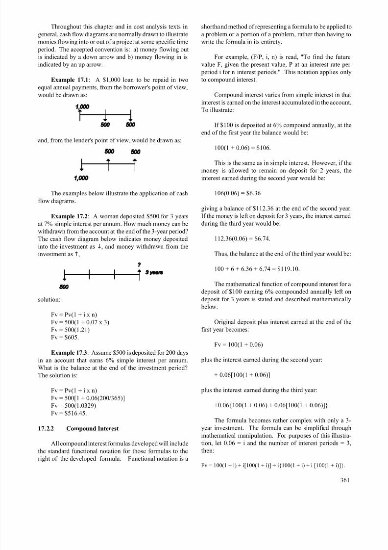
Throughout this chapter and in cost analysis texts in
general, cash flow diagrams are normally drawn to illustrate
monies flowing into or out of a project at some specific time
period. The accepted convention is: a) money flowing out
is indicated by a down arrow and b) money flowing in is
indicated by an up arrow.
Example 17.1: A $1,000 loan to be repaid in two
equal annual payments, from the borrower's point of view,
would be drawn as:
and, from the lender's point of view, would be drawn as:
The examples below illustrate the application of cashflow diagrams.
Example 17.2: A woman deposited $500 for 3 years
at 7% simple interest per annum. How much money can be
withdrawn from the account at the end of the 3-year period?
The cash flow diagram below indicates money deposited
into the investment as i, and money withdrawn from the
investment as h,
solution:
Fv = Pv(1 + i x n)
Fv = 500(1 + 0.07 x 3)
Fv = 500(1.21)
Fv = $605.
Example 17.3: Assume $500 is deposited for 200 days
in an account that earns 6% simple interest per annum.
What is the balance at the end of the investment period?
The solution is:
Fv = Pv(1 + i x n)
Fv = 500[1 + 0.06(200/365)]
Fv = 500(1.0329)
Fv = $516.45.
17.2.2 Compound Interest
All compound interest formulas developed will include
the standard functional notation for those formulas to the
right of the developed formula. Functional notation is a
shorthand method of representing a formula to be applied to
a problem or a portion of a problem, rather than having to
write the formula in its entirety.
For example, (F/P, i, n) is read, "To find the future
value F, given the present value, P at an interest rate per
period i for n interest periods." This notation applies only
to compound interest.
Compound interest varies from simple interest in thatinterest is earned on the interest accumulated in the account.
To illustrate:
If $100 is deposited at 6% compound annually, at the
end of the first year the balance would be:
100(1 + 0.06) = $106.
This is the same as in simple interest. However, if the
money is allowed to remain on deposit for 2 years, the
interest earned during the second year would be:
106(0.06) = $6.36
giving a balance of $112.36 at the end of the second year.
If the money is left on deposit for 3 years, the interest earned
during the third year would be:
112.36(0.06) = $6.74.
Thus, the balance at the end of the third year would be:
100 + 6 + 6.36 + 6.74 = $119.10.
The mathematical function of compound interest for a
deposit of $100 earning 6% compounded annually left on
deposit for 3 years is stated and described mathematically
below.
Original deposit plus interest earned at the end of the
first year becomes:
Fv = 100(1 + 0.06)
plus the interest earned during the second year:
+ 0.06[100(1 + 0.06)]
plus the interest earned during the third year:
+0.06{100(1 + 0.06) + 0.06[100(1 + 0.06)]}.
The formula becomes rather complex with only a 3-
year investment. The formula can be simplified through
mathematical manipulation. For purposes of this illustra-
tion, let 0.06 = i and the number of interest periods = 3,
then:
Fv = 100(1 + i) + i[100(1 + i)] + i{100(1 + i) + i [100(1 + i)]}.
361
8/12/2019 Costing & Analysis for Engineering
http://slidepdf.com/reader/full/costing-analysis-for-engineering 4/48
Factoring out $100 from the above equation:
Fv = 100[(1 + i) + i(1 +i) + i{(1 + i) + i(1 + i)}]
simplifying:
Fv = 100[1 + i + i + i2 + i(1 + i + i + i2)]
simplifying further:
Fv = 100(1 + i + i + i2 + i + i2 + i2 + i3)
and collecting terms:
Fv = 100(1 + 3i + 3i2 + i3)
then, this equation can be factored into:
Fv = 100[(1 + i)(1 + i)(1 + i)] = 100(1 + i)3.
Substituting n for the number of interest periods, which
in this case is 3, the result is:
Fv = 100(1 + i)n.
Letting Pv = the amount of the investment, then:
Fv = Pv(1 + i)n (F/P,i,n)(17.2)
This is the single payment compound amount factor.
Solving Equation (17.2) for Pv gives:
(P/F,i,n)(17.3)
which is the single payment present worth factor.
With the development of the equation for finding the
future value of a lump sum investment at a compound
interest rate for n interest periods, it can be shown how more
frequent compounding increases the interest earned.
An interest rate of 3%/6 mo would be stated in nominal
form as 6% compounded semiannually.
Consider the following examples with interest rates
stated as an annual percentage rate (APR), commonlyreferred to as the "nominal interest rate."
Example 17.4: An amount of $100 is invested for 3
years in an account that earns 18% compounded annually.
The future value at the end of the 3-year period will be:
Fv = Pv(1 + i)n
Fv = 100(1 + 0.18)3
Fv = 100(1.6430)
Fv = $164.30.
362
Example 17.5: Assume $100 is invested for three
years in an account that earns 18% compounded quarterly.
The future value at the end of the 3-year period is:
Fv = Pv(1 + i)n
where
i = 0.18/4 quarters/y = 0.045 per quarter
n = 3 y x 4 quarters/y = 12 interest periods.
Solution:
Fv = 100(1 + 0.045)12
Fv = 100(1.6959)
Fv = $169.59.
Example 17.6: Suppose $100 is invested in an account
that earns 18% compounded monthly. The future value at
the end of a 3-year period is:
Fv = Pv(1 + i)n
where
i = 0.18/12 months/y = 0.015/mo
n = 3 y x 12 mo/y = 36 interest periods.
Solution:
Fv = 100(1 + 0.015)36
Fv = 100(1.7091)
Fv = $170.91.
Example 17.7: An amount of $100 is invested for 3
years in an account that earns 18% compounded weekly.
The future value at the end of the 3-year period is:
Fv = Pv(1 + i)n
where
i = 0.18/52 weeks/y = 0.0034615/week
n = 3 y x 52 weeks/y = 156 weeks.
Solution:
Fv = 100(1 + 0.0034615)
156
Fv = 100(1.7144)
Fv = $171.44.
Example 17.8: If $100 is invested for 3 years in an
account that earns 18% compounded daily, the future value
at the end of the 3-year period is:
Fv = Pv(1 + i)n
8/12/2019 Costing & Analysis for Engineering
http://slidepdf.com/reader/full/costing-analysis-for-engineering 5/48
where
i = 0.18/365 days/y = 0.00049315/d
n = 3 y x 365 d/y = 1095 d.
Solution:
Fv = 100(1 + 0.00049315)1095
Fv = 100(1.71577)
Fv = $171.58.
Money invested today will grow to a larger amount in
the future. If this is true, then the promise to pay some
amount of money in the future is worth a smaller amount
today.
Example 17.9: What is the present value of a promise
to pay $3,000 5 years from today if the interest rate is 12%
compounded monthly? This can be written:
where
i = 0.12/12 = 0.01
n = 5 x 12 = 60.
Solution:
Pv = 3,000/(1 + 0.01)60
Pv = $1,651.35.
17.2.3 Annual Effective Interest Rates
It is convenient at this point in the development of
compound interest to introduce annual effective interest
rates. Annual effective interest (AEI) is interest stated in
terms of an annual rate compounded yearly, which is the
equivalent of a nominally stated interest rate. Table 17.1
illustrates the relationship between nominal interest, interest
rate per interest period, and annual effective interest.
Notice that the nominal interest rate remains the same
percentage while the compounding periods change. The
interest rate per interest period is obtained by dividing the
nominal rate by the number of interest periods per year. The
annual effective interest rate is the only true indicator of theamount of annual interest, and therefore, annual effective
interest provides a true measure for comparing interest rates
when the frequency of compounding is different.
The annual effective interest rate may be found for any
nominal interest rate as shown below.
Table 17.1 Comparative Interest Rates
______________________________________________
(APR) Nominal Interest Rate per Annual Effective
Interest Rate Interest Period Interest (AEI)
(18%) (%) (%)
Compound 18.00 18.00
annually
Compounded 9.00 18.81 semiannually
Compounded 4.50 19.25
quarterly
Compounded 1.50 19.56
monthly
Compounded 0.346 19.71
weekly
Compounded 0.04932 19.716
daily
Compounded 19.7217
continuously
______________________________________________
Consider a dollar that was invested for 1 year at a
nominal rate of 18% compounded monthly. To calculate the
balance (Fv) at the end of the year:
Fv = 1[1 + (0.18/12)]12
therefore,
Fv = 1(1.015)12
Fv = 1(1.1956)
Fv = $1.1956.
Because a dollar was invested originally, the annual
interest earned may be found by subtracting the original
investment:
1.1956 - 1 = 0.1956
and the effective interest is 19.56%. Then, the formula for finding annual effective interest is:
(17.4)
363

8/12/2019 Costing & Analysis for Engineering
http://slidepdf.com/reader/full/costing-analysis-for-engineering 6/48
where
AEI = annual effective interest rate
r = nominal interest rate/y
m = number of interest periods/y.
The annual percentage rate is divided by the number of
compounding periods/y and raised to the power of the
number of compounding periods/y, and 1 is subtracted from
that answer to arrive at the annual effective interest rate.
The following examples are used to further illustrate
the differences between APR and AEI.
Example 17.10: For an APR of 12% compounded
annually, the annual effective interest (AEI) is 12%.
Therefore:
AEI = 12% compounded annually. There is no
difference between the two.
Example 17.11: For an APR of 12% compounded
semi-annually, the semiannual effective interest rate is0.12/2 = 0.06 or 6%, presented as:
AEI = (1 + 0.12/2)2 - 1 = 0.1236 or 12.36%.
Example 17.12: For an APR of 12% compounded
quarterly, the quarterly effective interest rate is 0.03 or 3%,
AEI becomes:
AEI = (1 + 0.12/4)4 - 1 = 0.1255 or 12.55%.
Example 17.13: For an APR of 12% compounded
daily, the daily effective interest rate is 0.12/365 = 0.003288
or 0.3288%, giving:
AEI = (1 + 0.12/365)365 - 1 = 0.12747 or 12.75%.
When interest is compounded continuously (when n
approaches infinity), the annual effective interest rate takes
the form of e - 1, where e = the natural logarithm
2.7182818. Therefore, an APR of 12% compounded
continuously would yield an AEI of (2.7182818)0.12 - 1 =
12.749%.
Effective interest rates can be calculated for periods
other than annually.
To find a weekly effective interest rate of 12%
compounded daily, the weekly effective interest rate would
be:
(1 + 0.12/365)7 - 1 = 0.0023, or 0.23%.
Therefore,
(17.5)
364
where
r = annual percentage rate
m = number of compound periods/year
c = number of compound periods for the time frame
of the effective interest rate.
Example 17.14: The present value of a promise to pay
$4,000 6 years from today at an interest rate that is
compounded quarterly is $2,798. Find the nominal interestrate and the annual effective interest rate.
Fv = Pv(1 + i)n
where
n = 6 x 4 = 24 quarters
and solving
4,000 = 2,798(1 + i)24
dividing both sides by 2,798
1.42959 = (1 + i)24
taking the 24th root of both sides
(1.42959)0.04167 = [(1 + i)24]0.04167
1.015 = 1 + i
i = 0.015, or 1.5%.
By definition, i is the interest rate per interest period.
Therefore, the answer, 1.5%, is the interest rate per quarter.
In order to find the nominal interest rate (or annual
percentage rate), it is necessary to multiply i times the
number of quarters per year. The nominal interest rate is
0.015 x 4 = 0.06, or 6% compounded quarterly. The answer
would be incorrect if the frequency of compounding was not
included. If the nominal rate is given as 6%, this would
indicate 6% compounded annually.
The annual effective interest rate, using Equation
(17.4), becomes:
AEI = (1 + 0.015)4 - 1
AEI = 0.0614, or 6.14%.
8/12/2019 Costing & Analysis for Engineering
http://slidepdf.com/reader/full/costing-analysis-for-engineering 7/48
Years
5
10
15 20 25 3530 4010
20
30
40
50
60
70
80
90
100
4%
6%
8%
10%
12%
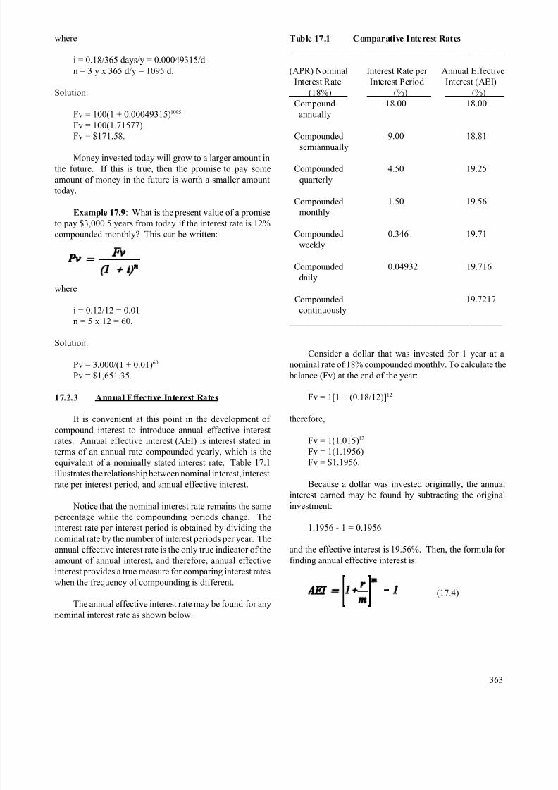
Figure 17.1 Exponential nature of compound interest rates.
The formulas developed for compound interest and thesimilar formula for converting APR to AEI are logarithmic
functions (see Figure 17.1).
When interest rates are extremely low, the number of
compounding periods is almost insignificant. For example,
2% APR compounded annually is 2% AEI; 2% APR
compounded daily is 2.02% AEI while 40% APR
compounded daily jumps to 49.15% AEI.
In evaluating projects for nonprofit organizations,
interest rates are usually kept rather low, but there are many
private entities that evaluate alternatives at the corporation’s
rate of return, which can be a very high rate.
17.3 ANNUITIES
17.3.1 Ordinary Annuities
The definition of an ordinary annuity is a stream of
equal end-of-period payments. Ordinary annuities are the
most common form of payment series used in cost analysis.
Loan payments, car payments, charge card payments,
maintenance and operating costs of equipment are all stated
in terms of ordinary annuities. These payments arefrequently monthly payments, but they can be weekly, yearly
or any other uniform time period. The important thing is
that they begin at the end of the first interest period. For
example, a person purchases an automobile for $5,000 and
is obligated to pay $125 per month for 48 months. The first
payment will be due one month after the purchase of the car
and the last payment will be due at the end of month 48. In
order to derive a mathematical formula to evaluate ordinary
annuities, it is convenient to use the future value formula for
compound interest Equation (17.2).
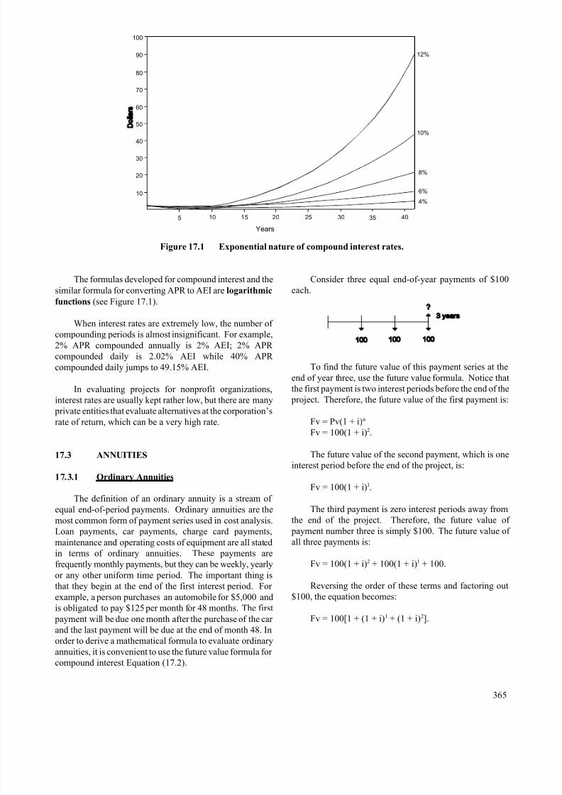
Consider three equal end-of-year payments of $100each.
To find the future value of this payment series at the
end of year three, use the future value formula. Notice that
the first payment is two interest periods before the end of the
project. Therefore, the future value of the first payment is:
Fv = Pv(1 + i)n
Fv = 100(1 + i)2.
The future value of the second payment, which is one
interest period before the end of the project, is:
Fv = 100(1 + i)1.
The third payment is zero interest periods away from
the end of the project. Therefore, the future value of
payment number three is simply $100. The future value of
all three payments is:
Fv = 100(1 + i)2 + 100(1 + i)1 + 100.
Reversing the order of these terms and factoring out
$100, the equation becomes:
Fv = 100[1 + (1 + i)1 + (1 + i)2].
365
8/12/2019 Costing & Analysis for Engineering
http://slidepdf.com/reader/full/costing-analysis-for-engineering 8/48
Notice that with a 3-year project and three annual
payments, n does not get higher than 2. This is because the
payments are made at the end of each period. Letting A =
the amount of each payment, a general equation can be
written to find the future value of n payments as:
Fv = A[1 + (1 + i)1 + (1 + i)2 + (1 + i)3 +...+ (1 + i)n-1].
Multiplying this equation by (1 + i) results in:
Fv(1 + i) = A[(1 + i)1 + (1 + i)2 + (1 + I)3
+ (1 + i)4 +...+ (1 + i)n].
Subtracting the first equation from the second equation:
Fv(1 + i) - Fv = A[-1 + (1 + i)n]
also
Fv + i(Fv) - Fv = A[(1 + i)n - 1]
and
i(Fv) = A[(1 + i)n - 1]
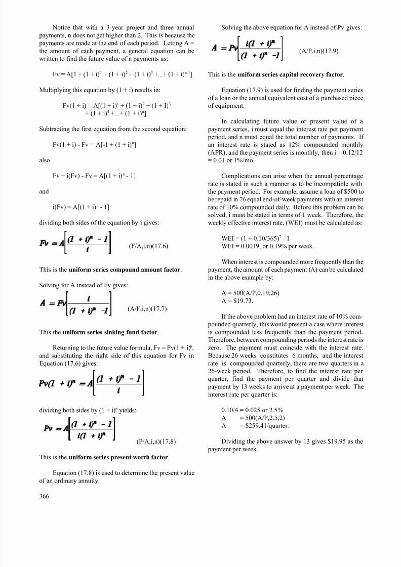
dividing both sides of the equation by i gives:
(F/A,i,n)(17.6)
This is the uniform series compound amount factor.
Solving for A instead of Fv gives:
(A/F,i,n)(17.7)
This the uniform series sinking fund factor.
Returning to the future value formula, Fv = Pv(1 + i)n,
and substituting the right side of this equation for Fv in
Equation (17.6) gives:
dividing both sides by (1 + i)n yields:
(P/A,i,n)(17.8)
This is the uniform series present worth factor.
Equation (17.8) is used to determine the present value
of an ordinary annuity.
366
Solving the above equation for A instead of Pv gives:
(A/P,i,n)(17.9)
This is the uniform series capital recovery factor.
Equation (17.9) is used for finding the payment series
of a loan or the annual equivalent cost of a purchased pieceof equipment.
In calculating future value or present value of a
payment series, i must equal the interest rate per payment
period, and n must equal the total number of payments. If
an interest rate is stated as 12% compounded monthly
(APR), and the payment series is monthly, then i = 0.12/12
= 0.01 or 1%/mo.
Complications can arise when the annual percentage
rate is stated in such a manner as to be incompatible with
the payment period. For example, assume a loan of $500 to
be repaid in 26 equal end-of-week payments with an interestrate of 10% compounded daily. Before this problem can be
solved, i must be stated in terms of 1 week. Therefore, the
weekly effective interest rate, (WEI) must be calculated as:
WEI = (1 + 0.10/365)7 - 1
WEI = 0.0019, or 0.19% per week.
When interest is compounded more frequently than the
payment, the amount of each payment (A) can be calculated
in the above example by:
A = 500(A/P,0.19,26)
A = $19.73.
If the above problem had an interest rate of 10% com-
pounded quarterly, this would present a case where interest
is compounded less frequently than the payment period.
Therefore, between compounding periods the interest rate is
zero. The payment must coincide with the interest rate.
Because 26 weeks constitutes 6 months, and the interest
rate is compounded quarterly, there are two quarters in a
26-week period. Therefore, to find the interest rate per
quarter, find the payment per quarter and divide that
payment by 13 weeks to arrive at a payment per week. The
interest rate per quarter is:
0.10/4 = 0.025 or 2.5%
A = 500(A/P,2.5,2)
A = $259.41/quarter.
Dividing the above answer by 13 gives $19.95 as the
payment per week.
8/12/2019 Costing & Analysis for Engineering
http://slidepdf.com/reader/full/costing-analysis-for-engineering 9/48
Returning to the problem at the beginning of 17.3.1
Ordinary Annuities, $5,000 was financed on an automobile
for 48 months at an interest rate of 9.24% compounded
monthly. Find the monthly payment:
where
i = 0.0924/12 = 0.0077
n = 4 x 12 = 48.
Solution
A = 5,000(A/P,0.77,48)
A = $124.996 or $125/mo.
17.3.2 Annuities Due
The definition of an annuity due is a stream of equal,
beginning-of-the-period payments. Although this payment
series is not nearly as common as an ordinary annuity, it is
still found in many projects. Beginning-of-the-period
payments apply to such things as rents, leases, insurance
premiums, subscriptions, etc. Rather than attempt to derivea formula to evaluate annuities due, it is much simpler to
modify the existing formulas that have already been derived.
Consider a 5-year cash flow diagram with payments made
at the beginning of each year. These payments will be
designated as (a) to avoid confusion with an ordinary
annuity. The diagram is shown as:
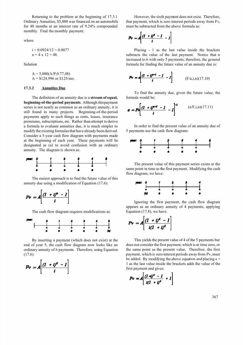
The easiest approach is to find the future value of this
annuity due using a modification of Equation (17.6):
The cash flow diagram requires modifications as:
By inserting a payment (which does not exist) at theend of year 5, the cash flow diagram now looks like an
ordinary annuity of 6 payments. Therefore, using Equation
(17.6):
However, the sixth payment does not exist. Therefore,
that payment, which is zero interest periods away from Fv,
must be subtracted from the above formula as:
Placing - 1 as the last value inside the brackets
subtracts the value of the last payment. Notice that n
increased to 6 with only 5 payments; therefore, the generalformula for finding the future value of an annuity due is:
(F/a,i,n)(17.10)
To find the annuity due, given the future value, the
formula would be:
(a/F,i,n)(17.11)
In order to find the present value of an annuity due of
5 payments use the cash flow diagram:
The present value of this payment series exists at the
same point in time as the first payment. Modifying the cash
flow diagram, we have:
Ignoring the first payment, the cash flow diagram
appears as an ordinary annuity of 4 payments, applying
Equation (17.8), we have:
This yields the present value of 4 of the 5 payments butdoes not consider the first payment, which is at time zero, or
the same point as the present value. Therefore, the first
payment, which is zero interest periods away from Pv, must
be added. By modifying the above equation and placing a +
1 as the last value inside the brackets adds the value of the
first payment and gives:
367
8/12/2019 Costing & Analysis for Engineering
http://slidepdf.com/reader/full/costing-analysis-for-engineering 10/48
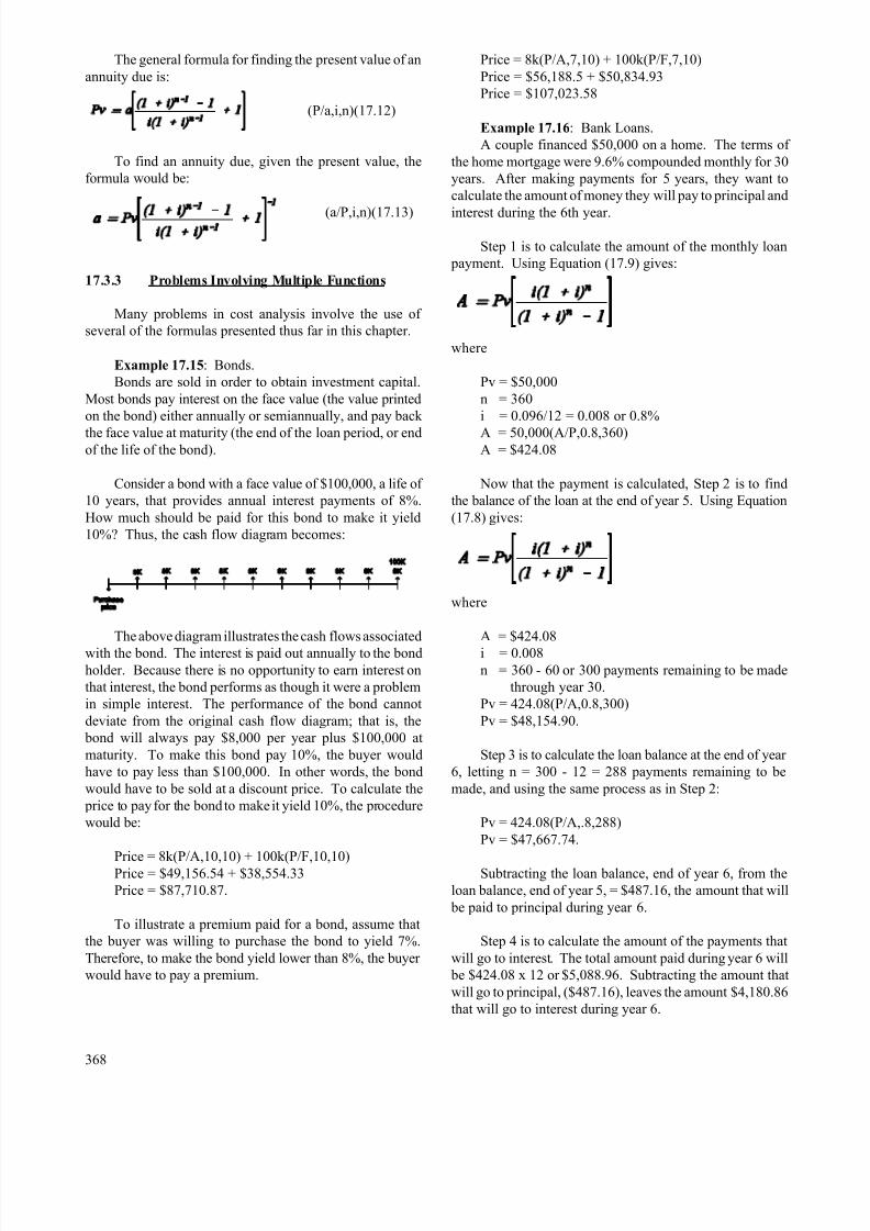
The general formula for finding the present value of an
annuity due is:
(P/a,i,n)(17.12)
To find an annuity due, given the present value, the
formula would be:
(a/P,i,n)(17.13)
17.3.3 Problems Involving Multiple Functions
Many problems in cost analysis involve the use of
several of the formulas presented thus far in this chapter.
Example 17.15: Bonds.
Bonds are sold in order to obtain investment capital.
Most bonds pay interest on the face value (the value printed
on the bond) either annually or semiannually, and pay back
the face value at maturity (the end of the loan period, or endof the life of the bond).
Consider a bond with a face value of $100,000, a life of
10 years, that provides annual interest payments of 8%.
How much should be paid for this bond to make it yield
10%? Thus, the cash flow diagram becomes:
The above diagram illustrates the cash flows associated
with the bond. The interest is paid out annually to the bond
holder. Because there is no opportunity to earn interest on
that interest, the bond performs as though it were a problem
in simple interest. The performance of the bond cannot
deviate from the original cash flow diagram; that is, the
bond will always pay $8,000 per year plus $100,000 at
maturity. To make this bond pay 10%, the buyer would
have to pay less than $100,000. In other words, the bond
would have to be sold at a discount price. To calculate the
price to pay for the bond to make it yield 10%, the procedure
would be:
Price = 8k(P/A,10,10) + 100k(P/F,10,10)Price = $49,156.54 + $38,554.33
Price = $87,710.87.
To illustrate a premium paid for a bond, assume that
the buyer was willing to purchase the bond to yield 7%.
Therefore, to make the bond yield lower than 8%, the buyer
would have to pay a premium.
368
Price = 8k(P/A,7,10) + 100k(P/F,7,10)
Price = $56,188.5 + $50,834.93
Price = $107,023.58
Example 17.16: Bank Loans.
A couple financed $50,000 on a home. The terms of
the home mortgage were 9.6% compounded monthly for 30
years. After making payments for 5 years, they want to
calculate the amount of money they will pay to principal and
interest during the 6th year.
Step 1 is to calculate the amount of the monthly loan
payment. Using Equation (17.9) gives:
where
Pv = $50,000
n = 360
i = 0.096/12 = 0.008 or 0.8%
A = 50,000(A/P,0.8,360)A = $424.08
Now that the payment is calculated, Step 2 is to find
the balance of the loan at the end of year 5. Using Equation
(17.8) gives:
where
A = $424.08
i = 0.008
n = 360 - 60 or 300 payments remaining to be made
through year 30.
Pv = 424.08(P/A,0.8,300)
Pv = $48,154.90.
Step 3 is to calculate the loan balance at the end of year
6, letting n = 300 - 12 = 288 payments remaining to be
made, and using the same process as in Step 2:
Pv = 424.08(P/A,.8,288)
Pv = $47,667.74.
Subtracting the loan balance, end of year 6, from the
loan balance, end of year 5, = $487.16, the amount that will
be paid to principal during year 6.
Step 4 is to calculate the amount of the payments that
will go to interest. The total amount paid during year 6 will
be $424.08 x 12 or $5,088.96. Subtracting the amount that
will go to principal, ($487.16), leaves the amount $4,180.86
that will go to interest during year 6.
8/12/2019 Costing & Analysis for Engineering
http://slidepdf.com/reader/full/costing-analysis-for-engineering 11/48
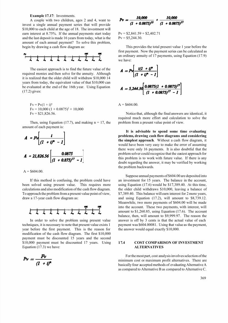
Example 17.17: Investments.
A couple with two children, ages 2 and 4, want to
invest a single annual payment series that will provide
$10,000 to each child at the age of 18. The investment will
earn interest at 8.75%. If the annual payments start today
and the last deposit is made 16 years from today, what is the
amount of each annual payment? To solve this problem,
begin by drawing a cash flow diagram as:
The easiest approach is to find the future value of the
required monies and then solve for the annuity. Although
it is realized that the older child will withdraw $10,000 14
years from today, the equivalent value of that $10,000 can
be evaluated at the end of the 16th year. Using Equation
(17.2) gives:
Fv = Pv(1 + i)n
Fv = 10,000 (1 + 0.0875)2 + 10,000
Fv = $21,826.56.
Then, using Equation (17.7), and making n = 17, the
amount of each payment is:
A = $604.00.
If this method is confusing, the problem could have
been solved using present value. This requires more
calculations and also modification of the cash flow diagram.
To approach the problem from a present value point of view,
draw a 17-year cash flow diagram as:
In order to solve the problem using present value
techniques, it is necessary to note that present value exists 1year before the first payment. This is the reason for
modification of the cash flow diagram. The first $10,000
payment must be discounted 15 years and the second
$10,000 payment must be discounted 17 years. Using
Equation (17.3) we have:
Pv = $2,841.59 + $2,402.71
Pv = $5,244.30.
This provides the total present value 1 year before the
first payment. Now the payment series can be calculated as
an ordinary annuity of 17 payments, using Equation (17.9)we have:
A = $604.00.
Notice that, although the final answers are identical, itrequired much more effort and calculation to solve the
problem from a present value point of view.
It is advisable to spend some time evaluating
problems, drawing cash flow diagrams and considering
the simplest approach. Without a cash flow diagram, it
would have been very easy to make the error of assuming
there were only 16 payments. It is also doubtful that the
problem solver could recognize that the easiest approach for
this problem is to work with future value. If there is any
doubt regarding the answer, it may be verified by working
the problem backwards.
Suppose annual payments of $604.00 are deposited into
an investment for 15 years. The balance in the account,
using Equation (17.6) would be $17,389.40. At this time,
the older child withdraws $10,000, leaving a balance of
$7,389.40. This balance will earn interest for 2 more years,
and using Equation (17.2), will amount to $8,739.12.
Meanwhile, two more payments of $604.00 will be made
into the account. These two payments, with interest, will
amount to $1,260.85, using Equation (17.6). The account
balance, then, will amount to $9,999.97. The reason the
answer is off by 3 cents is that the actual value of each
payment was $604.00081. Using that value as the payment,the answer would equal exactly $10,000.
17.4 COST COMPARISON OF INVESTMENT
ALTERNATIVES
For the most part, cost analysis involves selection of the
minimum cost or maximum profit alternatives. There are
basically four accepted methods of evaluating Alternative A
as compared to Alternative B as compared to Alternative C.
369
8/12/2019 Costing & Analysis for Engineering
http://slidepdf.com/reader/full/costing-analysis-for-engineering 12/48
17.4.1 Present Value Method
The first of these methods is the present value
technique, wherein all costs and revenues are discounted
back to present value to arrive at a net present value for the
project. This method is very time consuming if performed
manually and presents problems when the alternatives have
different economic lives. Alternative A may have an
expected life of 10 years, Alternative B may have an
expected life of 15 years, and Alternative C may have anexpected life of 20 years. Therefore, in order to do any
meaningful evaluation of these three alternatives in terms of
present value, it is necessary to find a common denominator
for their expected life, which, in this case, would be 60 years,
where Alternative A would be replaced six times, B replaced
four times, and C replaced three times.
17.4.2 Future Value Technique
The future value technique of evaluating alternatives is
almost identical to the present value method except that all
costs and revenues are stated in terms of future value. The
problem still arises of alternatives with incompatible usefullives. The above techniques are self-explanatory, and
because they require such extensive calculations, they will
not be covered further. But, because they exist, when
evaluating alternatives using computers, it is convenient to
indicate, somewhere in the output data generated, the net
present value (NPV) of each alternative. Many
organizations base their decisions on NPV, and
governmental agencies, expect to evaluate benefit-cost ratios.
The benefit-cost ratio is the ratio of benefits provided by the
alternative versus cost incurred, and will be discussed later
in this chapter.
17.4.3 Annual Equivalent Cost Method
The annual equivalent cost method of evaluating
alternative projects states all costs and revenues over
the useful life of the project in terms of an equal annual
payment series (an ordinary annuity). This is probably the
most widely used method in the industry, for several reasons:
1. It requires less effort and fewer calculations.
2. It eliminates the problem of alternatives with
incompatible useful lives.
3. It allows for much more sophistication when
considering inflation, increasing equipment cost,
equipment depreciation schedules, etc.
The annual cost method assumes that the project will
live forever, and that, if Alternative A has a useful life of 10
years and Alternative B has a useful life of 15 years, each
alternative will be replaced at the end of its useful life.
Therefore, the alternative with the minimum annual cost or
maximum annual profit is the alternative that will be chosen.
370
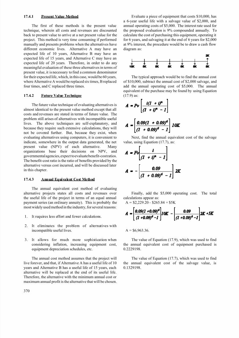
Evaluate a piece of equipment that costs $10,000, has
a 6-year useful life with a salvage value of $2,000, and
annual operating costs of $5,000. The interest rate used for
the proposed evaluation is 9% compounded annually. To
calculate the cost of purchasing this equipment, operating it
for 6 years, and salvaging it at the end of 6 years for $2,000
at 9% interest, the procedure would be to draw a cash flow
diagram as:
The typical approach would be to find the annual cost
of $10,000, subtract the annual cost of $2,000 salvage, and
add the annual operating cost of $5,000. The annual
equivalent of the purchase may be found by using Equation
(17.9) as:
Next, find the annual equivalent cost of the salvage
value, using Equation (17.7), as:
Finally, add the $5,000 operating cost. The total
calculations appear as:
A = $2,229.20 - $265.84 + $5K
A = $6,963.36.
The value of Equation (17.9), which was used to find
the annual equivalent cost of equipment purchased is
0.2229198.
The value of Equation (17.7), which was used to find
the annual equivalent cost of the salvage value, is
0.1329198.
8/12/2019 Costing & Analysis for Engineering
http://slidepdf.com/reader/full/costing-analysis-for-engineering 13/48
Notice that the difference between 0.2229198 and
0.1329198 is exactly equal to the interest rate (i), 0.09. This
is true for all interest rates, provided that these functions
have the same i and the same n.
In calculating the annual equivalent cost of purchasing
the equipment and subtracting the annual equivalent cost of
the equipment salvage at some time in the future, this is
always the case: i and n are equal; and Equation (17.9) - i
= Equation (17.7).
Using functional notation as symbols for these formulas
we have:
[(A/P,9,6) - 0.09] = (A/F,9,6).
Making this substitution, the annual cost formula
becomes:
A = (A/P,9,6)10K - [(A/P,9,6) - 0.09]2K + 5K
multiplying,
A = (A/P,9,6)10K - (A/P,9,6)2K + 0.09(2K) + 5K
factoring out (A/P,9,6),
A = (A/P,9,6)(10K - 2K) + 0.09(2K) +5K
the general equation for the annual cost equation becomes:
then
A = (A/P,i,n)(cost - salvage) + i(salvage) + OC (17.14)
represents the annual equivalent cost formula
where
OC = annual operating cost.
This modification of the annual cost formula greatly
reduces the amount of calculation necessary to arrive at the
annual equivalent cost.
Values can be produced by this formula as monthly
equivalent costs or weekly equivalent costs by simply
changing i to the interest rate per period and allowing n to
equal the total number of periods. Using the previous
example, suppose the annual percentage rate was 9%
compounded monthly. To calculate the periodic costs in
terms of monthly equivalent costs (as a monthly ordinary
annuity):
A = (A/P,0.75,72)(10K - 2K) + 0.0075(2K) + 5K/12
A = $144.20 + $15.00 + $416.67
A = $575.87.
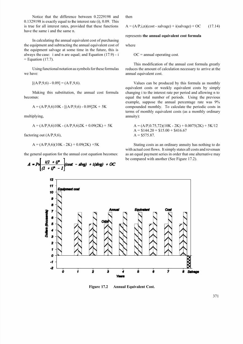
Stating costs as an ordinary annuity has nothing to do
with actual cost flows. It simply states all costs and revenues
as an equal payment series in order that one alternative may
be compared with another (See Figure 17.2).
Figure 17.2 Annual Equivalent Cost.
371
8/12/2019 Costing & Analysis for Engineering
http://slidepdf.com/reader/full/costing-analysis-for-engineering 14/48
17.4.4 Rate of Return Method
The rate of return (ROR) method of comparing
alternatives calculates the interest rate for each alternative
and selects the highest ROR. A word of caution is
necessary, ROR evaluates INVESTED capital and the costs
of operation and maintenance as opposed to revenues or
benefits received from the project. Therefore, a project
totally financed with borrowed money has no rate of return
because there is no invested capital. The followingexamples assume 100% equity financing and are used to
illustrate rate of return calculations.
Example 17.18: An investment of $7,000 is placed
into an account for a 10-year period. At the end of 10 years,
the balance in the account is $17,699.30. What was the
annual interest rate earned? Using Equation (17.2):
Fv = Pv(1 + i)n
$17,699.30 = $7,000(1 + i)10.
This problem can be solved by dividing both sides of the equation by $7,000 giving:
17,699.30/7,000 = (1 + i)10
2.528 = (1 + i)10.
Extracting the tenth root of each side of the equation
gives:
(2.528)0.1 = [(1 + i)10]0.1
1.0972 = 1 + i
i = 0.0972.
A ROR can also be calculated by evaluating the
difference between alternatives that provide cost savings
rather than revenues.
Example 17.19: Fire insurance premiums on a ware-
house are $500/y (Alternative A). The same coverage can
be purchased by paying a 3-year premium of $1,250
(Alternative B). Find the ROR realized by purchasing a 3-
year policy in place of three 1-year policies.
To simplify this problem, notice that the 3-year
insurance premium is 2.5 times the annual premium. The
cash flow diagram for Alternative A appears below.
The cash flow diagram for Alternative B appears
below.
372
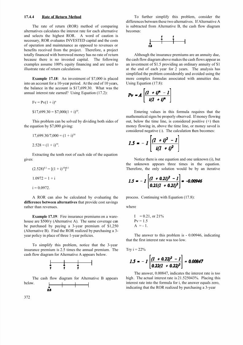
To further simplify this problem, consider the
differences between these two alternatives. If Alternative A
is subtracted from Alternative B, the cash flow diagram
becomes:
Although the insurance premiums are an annuity due,
the cash flow diagram above makes the cash flows appear asan investment of $1.5 providing an ordinary annuity of $1
at the end of each year for 2 years. The analysis has
simplified the problem considerably and avoided using the
more complex formulas associated with annuities due.
Using Equation (17.8):
Entering values in this formula requires that the
mathematical signs be properly observed. If money flowing
out, below the time line, is considered positive (+) thenmoney flowing in, above the time line, or money saved is
considered negative (-). The calculation then becomes:
Notice there is one equation and one unknown (i), but
the unknown appears three times in the equation.
Therefore, the only solution would be by an iterative
process. Continuing with Equation (17.8):
where
I = 0.21, or 21%
Pv = 1.5
A = - 1.
The answer to this problem is - 0.00946, indicating
that the first interest rate was too low.
Try i = 22%
The answer, 0.00847, indicates the interest rate is too
high. The actual interest rate is 21.525043%. Placing this
interest rate into the formula for i, the answer equals zero,
indicating that the ROR realized by purchasing a 3-year
8/12/2019 Costing & Analysis for Engineering
http://slidepdf.com/reader/full/costing-analysis-for-engineering 15/48
policy instead of three 1-year policies is 21.5%. There are
many pocket calculators costing under $20 that are designed
to calculate financial functions and are capable of iterating
for problems involving a single financial function.
Consider the annual cost formula where:
a = (A/P,i,n) x ( cost - salvage) + (i) salvage + OC - revenues.
Suppose it is required to find the ROR on such a project. Once again, the solution to the problem is found by
iteration. But in this case, there is more than one financial
function. Choose an interest rate. Work the problem at that
interest rate, and find out if the answer comes out positive or
negative. With the mathematical signs we have used in this
example, if revenues exceed costs the answer would be
negative; if costs exceed revenues the answer would be
positive. When the exact i is placed into the formula that
denotes the ROR, the answer would be zero. That is, the
interest rate that causes revenues and costs to be exactly
equal. Interest tables may be used to help find an upper and
lower range for i to reduce the number of iterations
necessary.
A much easier solution is to place all of the cash flows
by year into a computer and write a simple program that can
do thousands of iterations in a matter of seconds to find i.
Trying to iterate i for a problem with more than one
function on a financial calculator nearly always results in
error because of the tremendous amount of time and data
that must be entered by hand. Even with a computer
program, if the cash flows turn from negative to positive and
back to negative during the project life, i can take on the
form of a quadratic equation and the computer is unable to
determine whether i is positive or negative. There are
computer spreadsheets and other software available for
iterating i, but these have their limitations. One of the most
popular and widely used spread-sheets is designed to iterate
i for a series of cash flows. However, this spreadsheet
requires a rather accurate guess for i; because, if it does not
find i after 20 iterations, the resultant answer is "Err"
(error). The RELCOST program developed to accomplish
LCC analysis (copyright, Washington State Energy Office)
will iterate i to seven decimal places in a matter of seconds
for projects with over 150 input variables and more than 500
inflation rates, and evaluate the iterated i to determine
whether it is positive or negative. This program will bediscussed in more detail in Subsection 17.7, entitled "LIFE
CYCLE COST ANALYSIS."
17.5 GRADIENTS
17.5.1 Arithmetic Gradients
Having developed formulas for equal payment series
involving both ordinary annuities and annuities due, an end-
of-period payment series that increases by a fixed dollar
amount at the end of each period can now be evaluated.
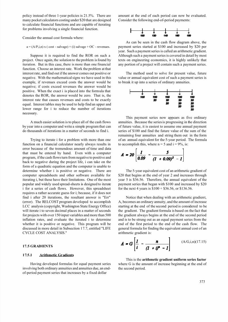
Consider the following end-of-period payments:
As can be seen in the cash flow diagram above, the
payment series started at $100 and increased by $20 per
year. Such a payment series is called an arithmetic gradient.
Although such a payment series is covered in detail by mosttexts on engineering economics, it is highly unlikely that
any portion of a project will contain such a payment series.
The method used to solve for present value, future
value or annual equivalent cost of such a payment series is
to break it up into a series of ordinary annuities.
This payment series now appears as five ordinary
annuities. Because the series is progressing in the direction
of future value, it is easiest to assume one annual payment
series of $100 and find the future value of the sum of the
remaining four annuities and string them out in the form
of an annual equivalent for the 5-year period. The formula
to accomplish this, where n = 5 and i = 9%, is:
The 5-year equivalent cost of an arithmetic gradient of
$20 that begins at the end of year 2 and increases through
year 5 is $36.56. Therefore, the annual equivalent of the
payment series that began with $100 and increased by $20
for the next 4 years is $100 + $36.56, or $136.56.
Notice that when dealing with an arithmetic gradient,
A1 becomes an ordinary annuity, and the amount of increase
starting at the end of the second period is considered to be
the gradient. The gradient formula is based on the fact that
the gradient always begins at the end of the second period
and is to be strung out as an equal payment series from the
end of the first period to the end of the cash flow. Thegeneral formula for finding the equivalent annual cost of an
arithmetic gradient is:
(A/G,i,n)(17.15)
This is the arithmetic gradient uniform series factor
where G is the amount of increase beginning at the end of
the second period.
373
8/12/2019 Costing & Analysis for Engineering
http://slidepdf.com/reader/full/costing-analysis-for-engineering 16/48
If the present value or future value of an arithmetic
gradient is required, one could simply multiply Equation
(17.15) by (P/A,i,n) or (F/A,i,n).
The most common use of arithmetic gradients is in
calculating the value of sum-of-years-digits (S-Y-D)
depreciation, which takes the form of a negative arithmetic
gradient. This method of depreciation is no longer allowed
under the 1987 tax law.
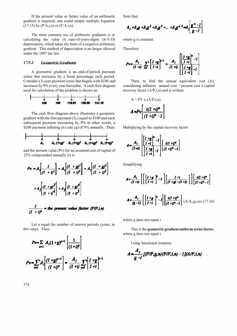
17.5.2 Geometric Gradients
A geometric gradient is an end-of-period payment
series that increases by a fixed percentage each period.
Consider a 5-year payment series that begins with $100 and
increases by 9% every year thereafter. A cash flow diagram
used for calculation of the problem is shown as:
The cash flow diagram above illustrates a geometric
gradient with the first payment (A1) equal to $100 and eachsubsequent payment increasing by 9% in other words, a
$100 payment inflating at a rate (g) of 9% annually. Then:
and the present value (Pv) for an assumed cost of capital of
12% compounded annually (i) is:
Let n equal the number of interest periods (years, in
this case). Then:
374
Note that:
where g is constant.
Therefore:
Then, to find the annual equivalent cost (A),
considering inflation: annual cost = present cost x capital
recovery factor (A/P,i,n) and is written:
A = PV x (A/P,i,n)
Multiplying by the capital recovery factor:
Simplifying:
(A/A1,g,i,n) (17.16)
where g does not equal i.
This is the geometric gradient uniform series factor,
where g does not equal i.
Using functional notation:
8/12/2019 Costing & Analysis for Engineering
http://slidepdf.com/reader/full/costing-analysis-for-engineering 17/48
Inserting the initial values in this example:
(0.2774) = $117.38.
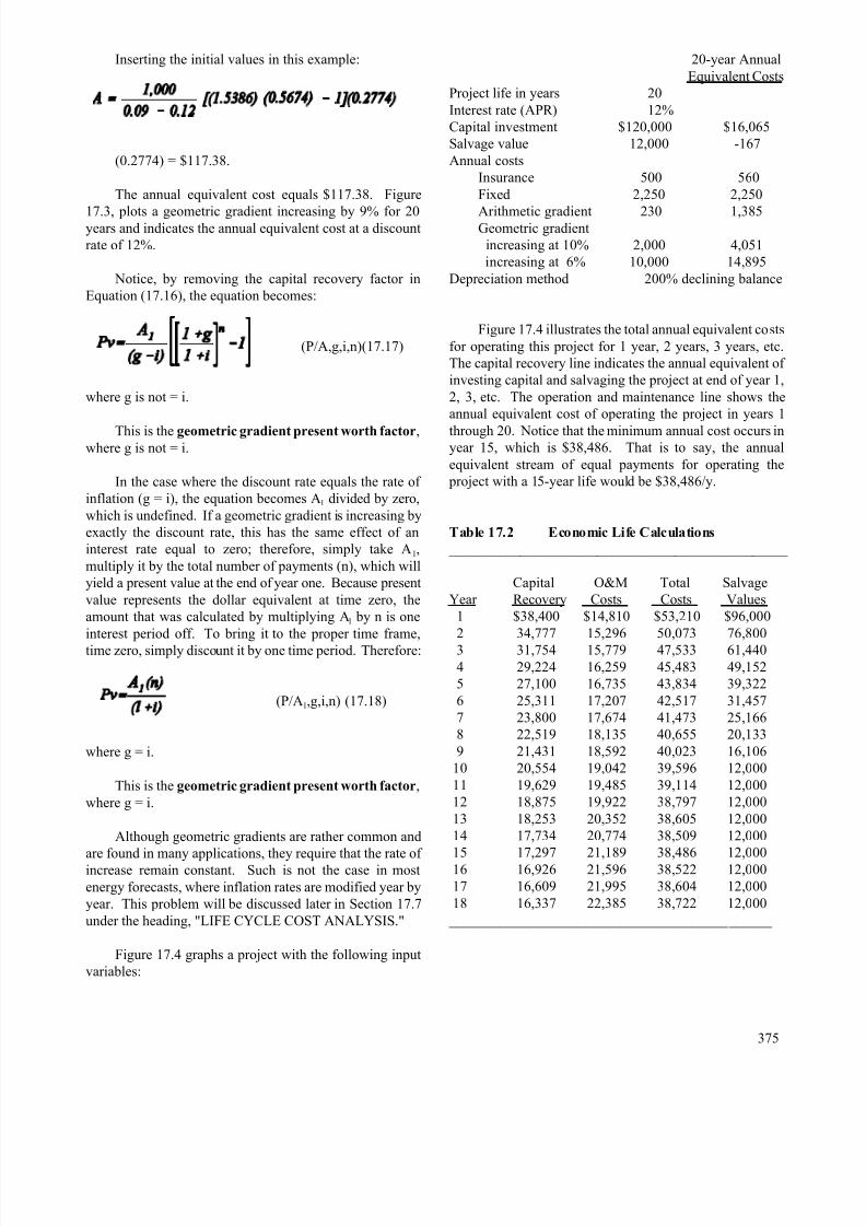
The annual equivalent cost equals $117.38. Figure
17.3, plots a geometric gradient increasing by 9% for 20years and indicates the annual equivalent cost at a discount
rate of 12%.
Notice, by removing the capital recovery factor in
Equation (17.16), the equation becomes:
(P/A,g,i,n)(17.17)
where g is not = i.
This is the geometric gradient present worth factor,where g is not = i.
In the case where the discount rate equals the rate of
inflation (g = i), the equation becomes A1 divided by zero,
which is undefined. If a geometric gradient is increasing by
exactly the discount rate, this has the same effect of an
interest rate equal to zero; therefore, simply take A1,
multiply it by the total number of payments (n), which will
yield a present value at the end of year one. Because present
value represents the dollar equivalent at time zero, the
amount that was calculated by multiplying A1 by n is one
interest period off. To bring it to the proper time frame,
time zero, simply discount it by one time period. Therefore:
(P/A1,g,i,n) (17.18)
where g = i.
This is the geometric gradient present worth factor,
where g = i.
Although geometric gradients are rather common and
are found in many applications, they require that the rate of increase remain constant. Such is not the case in most
energy forecasts, where inflation rates are modified year by
year. This problem will be discussed later in Section 17.7
under the heading, "LIFE CYCLE COST ANALYSIS."
Figure 17.4 graphs a project with the following input
variables:
20-year Annual
Equivalent Costs
Project life in years 20
Interest rate (APR) 12%
Capital investment $120,000 $16,065
Salvage value 12,000 -167
Annual costs
Insurance 500 560
Fixed 2,250 2,250
Arithmetic gradient 230 1,385Geometric gradient
increasing at 10% 2,000 4,051
increasing at 6% 10,000 14,895
Depreciation method 200% declining balance
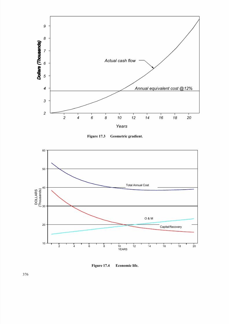
Figure 17.4 illustrates the total annual equivalent costs
for operating this project for 1 year, 2 years, 3 years, etc.
The capital recovery line indicates the annual equivalent of
investing capital and salvaging the project at end of year 1,
2, 3, etc. The operation and maintenance line shows the
annual equivalent cost of operating the project in years 1
through 20. Notice that the minimum annual cost occurs inyear 15, which is $38,486. That is to say, the annual
equivalent stream of equal payments for operating the
project with a 15-year life would be $38,486/y.
Table 17.2 Economic Life Calculations
________________________________________________
Capital O&M Total Salvage
Year Recovery Costs Costs Values
1 $38,400 $14,810 $53,210 $96,000
2 34,777 15,296 50,073 76,800
3 31,754 15,779 47,533 61,440
4 29,224 16,259 45,483 49,152
5 27,100 16,735 43,834 39,322
6 25,311 17,207 42,517 31,457
7 23,800 17,674 41,473 25,166
8 22,519 18,135 40,655 20,133
9 21,431 18,592 40,023 16,106
10 20,554 19,042 39,596 12,000
11 19,629 19,485 39,114 12,000
12 18,875 19,922 38,797 12,000
13 18,253 20,352 38,605 12,000
14 17,734 20,774 38,509 12,000
15 17,297 21,189 38,486 12,000 16 16,926 21,596 38,522 12,000
17 16,609 21,995 38,604 12,000
18 16,337 22,385 38,722 12,000
_____________________________________________
375
8/12/2019 Costing & Analysis for Engineering
http://slidepdf.com/reader/full/costing-analysis-for-engineering 18/48
Years
2 4 6 8 10 12 14 16 18 20
3
5
4
6
4
2
7
8
9
Actual cash flow
Annual equivalent cost @12%
10
20
30
40
50
60
D O L L A R S
( T h o u s a n d s )
2 4 6 8 10 12 14 16 18 20YEARS
Capital Recovery
Total Annual Cost
O & M
Figure 17.3 Geometric gradient.
Figure 17.4 Economic life.
376
8/12/2019 Costing & Analysis for Engineering
http://slidepdf.com/reader/full/costing-analysis-for-engineering 19/48
Table 17.2 provides annual equivalent values from year
1 through year 18 for capital recovery, operation and
maintenance costs, and total annual costs. Salvage values
for any given year are indicated in the last column. This
analysis is beyond the scope of this chapter, but could be
used to determine the economic life (minimum annual cost)
of a project that had these cost characteristics. Table 17.2
provides answers for various costs that could be beneficial to
those who want to sharpen their expertise in calculating
capital recovery, annuities due, ordinary annuities,geometric gradients, and arithmetic gradients.
17.6 EQUIPMENT DEPRECIATION
A discussion of equipment depreciation is essential in
evaluating projects for taxable entities because equipment
depreciation significantly lowers the annual cost of a project.
This subject is also the area of constant change because it
changes as tax laws are revised. The amount of total capital
investment in a project and the reduction in tax liability
caused by depreciation or investment and energy tax credits
or both, all have a major bearing on whether or not the project is economically feasible. However, the 1986 tax law
drastically reduced many of these incentives. Competent tax
accountants should be a part of the development team to
ensure proper utilization of these considerations.
17.6.1 Straight Line Depreciation
Straight line depreciation is the simplest form of
depreciation and has survived tax law changes for many
decades and it is accepted by the 1987 tax law. The formula
for straight line depreciation is:
Life can be expressed in years, months, units of
production, operating hours, or miles. Under the 1987 tax
law, salvage values are set to zero.
17.6.2 Sum-of-Years Digits Depreciation
This depreciation method is an accelerated depreciation
schedule that recovers larger amounts of depreciation in the
early life of the asset. The method of calculation is as
follows:
1. Find the sum of the years' digits of the life of the
equipment. Example: For a 10-year life, the sum of
the digits 1 through 10 is equal to 55. The easiest way
to make this calculation is:
in this case,
2. This sum is then divided into cost minus salvage to
obtain one unit of depreciation, which is:
Example: Equipment cost = $60,000
Salvage value = $ 5,000
then,
3. This unit of depreciation is then multiplied by the years
of life in descending order, that is:
year 1 = 10 units = $10,000
year 2 = 9 units = $ 9,000
year 3 = 8 units = $ 8,000------ -- -- --------- -- ---------
year 10 = 1 unit = $ 1,000.
The depreciation charge under this method performs
like a negative arithmetic gradient where A1 is
$10,000 and G is -$1,000.
Although this method of depreciation is accepted
accounting practice and may be used on equipment
purchased before 1980, it is no longer allowed under
the 1987 tax law and is only discussed to illustrate an
application of the arithmetic gradient.
17.6.3 Declining Balance Depreciation
This method of depreciation is also an accelerated form
and may obtain even larger depreciation in the early life
than S-Y-D. With 200% declining balance depreciation, the
annual rate is 200% times the straight line rate. As an
example:
An asset with a 10-year life has a straight line rate of
1/10. Therefore, the 200% declining balance rate
would be 2/10 or 20%.
This rate is applied to the book value of the asset,
where book value equals cost minus accumulated
depreciation. Any salvage value of the equipment was
not considered except that the tax code provided that
the equipment could not be depreciated below its
salvage value. The $60,000 piece of equipment in the
example above would be evaluated using 200%
declining balance as shown in Table 17.3.
377
8/12/2019 Costing & Analysis for Engineering
http://slidepdf.com/reader/full/costing-analysis-for-engineering 20/48
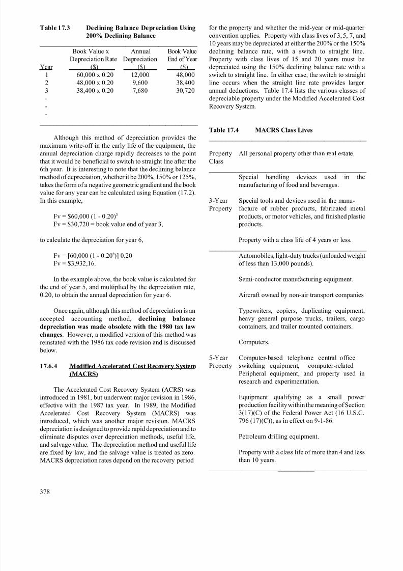
Table 17.3 Declining Balance Depreciation Using
200% Declining Balance
________________________________________________
Book Value x Annual Book Value
Depreciation Rate Depreciation End of Year
Year ($) ($) ($)
1 60,000 x 0.20 12,000 48,000
2 48,000 x 0.20 9,600 38,400
3 38,400 x 0.20 7,680 30,720
- -
-
________________________________________________
Although this method of depreciation provides the
maximum write-off in the early life of the equipment, the
annual depreciation charge rapidly decreases to the point
that it would be beneficial to switch to straight line after the
6th year. It is interesting to note that the declining balance
method of depreciation, whether it be 200%, 150% or 125%,
takes the form of a negative geometric gradient and the book
value for any year can be calculated using Equation (17.2).
In this example,
Fv = $60,000 (1 - 0.20)3
Fv = $30,720 = book value end of year 3,
to calculate the depreciation for year 6,
Fv = [60,000 (1 - 0.205)] 0.20
Fv = $3,932,16.
In the example above, the book value is calculated for
the end of year 5, and multiplied by the depreciation rate,
0.20, to obtain the annual depreciation for year 6.
Once again, although this method of depreciation is an
accepted accounting method, declining balance
depreciation was made obsolete with the 1980 tax law
changes. However, a modified version of this method was
reinstated with the 1986 tax code revision and is discussed
below.
17.6.4 Modified Accelerated Cost Recovery System
(MACRS)
The Accelerated Cost Recovery System (ACRS) was
introduced in 1981, but underwent major revision in 1986,effective with the 1987 tax year. In 1989, the Modified
Accelerated Cost Recovery System (MACRS) was
introduced, which was another major revision. MACRS
depreciation is designed to provide rapid depreciation and to
eliminate disputes over depreciation methods, useful life,
and salvage value. The depreciation method and useful life
are fixed by law, and the salvage value is treated as zero.
MACRS depreciation rates depend on the recovery period
378
for the property and whether the mid-year or mid-quarter
convention applies. Property with class lives of 3, 5, 7, and
10 years may be depreciated at either the 200% or the 150%
declining balance rate, with a switch to straight line.
Property with class lives of 15 and 20 years must be
depreciated using the 150% declining balance rate with a
switch to straight line. In either case, the switch to straight
line occurs when the straight line rate provides larger
annual deductions. Table 17.4 lists the various classes of
depreciable property under the Modified Accelerated CostRecovery System.
Table 17.4 MACRS Class Lives
________________________________________________
Property All personal property other than real estate.
Class
________________________________________________
Special handling devices used in the
manufacturing of food and beverages.
3-Year Special tools and devices used in the manu-Property facture of rubber products, fabricated metal
products, or motor vehicles, and finished plastic
products.
Property with a class life of 4 years or less.
________________________________________________
Automobiles, light-duty trucks (unloaded weight
of less than 13,000 pounds).
Semi-conductor manufacturing equipment.
Aircraft owned by non-air transport companies
Typewriters, copiers, duplicating equipment,
heavy general purpose trucks, trailers, cargo
containers, and trailer mounted containers.
Computers.
5-Year Computer-based telephone central office
Property switching equipment, computer-related
Peripheral equipment, and property used in
research and experimentation.
Equipment qualifying as a small power production facility within the meaning of Section
3(17)(C) of the Federal Power Act (16 U.S.C.
796 (17)(C)), as in effect on 9-1-86.
Petroleum drilling equipment.
Property with a class life of more than 4 and less
than 10 years.
________________________________________________
8/12/2019 Costing & Analysis for Engineering
http://slidepdf.com/reader/full/costing-analysis-for-engineering 21/48
Table 17.4 MACRS Class Lives (continued)
________________________________________________
Property All personal property other than real estate.
Class
______________________________________________
All property not assigned by law to another
class.
Any railroad track.
7-Year Office furniture, equipment, and fixtures.
Property Cellular phones, fax machines, refrigerators,
dishwashers. Machines used to produce
jewelry, toys, musical instruments, and
sporting goods.
Single-purpose agricultural or horticultural
structures placed in service in 1987 or 1988.
Property with a class life of 10 years or more,
but less than 16 years.
_______________________________________________
Equipment used in the refining of petroleum,
the manufacture of tobacco products andcertain food products.
Railroad cars.
10-Year
Property Water transportation equipment and vessels.
Single-purpose agricultural or horticultural
structures place in service after 1988.
Property with a class life of 16 years or more,
but less than 20 years.
________________________________________________
Land improvements such as fences, shrubbery,
roads, and bridges.
Any municipal waste water treatment plant.
15-Year Telephone distribution plants and equipment
Property used for 2-way exchange of voice and data
communications.
Property with a class life of 20 years or more,
but less than 25 years.
________________________________________________
Farm buildings.
20-Year Municipal sewers.
Property
Property with a class life of 25 years or more.
________________________________________________
27.5-Year Residential rental property (excluding hotels
Property and motels) placed in service after December
31, 1986.
________________________________________________
31.5 Year Non-residential real property placed in
Property service after December 31, 1986, but before
May 13, 1993.
________________________________________________
39-Year Non-residential property placed in service
Property after May 12, 1993.
________________________________________________
The mid-year convention treats all property acquired
during the year as though it were acquired in mid-year and
only half of the first year depreciation is allowed. Similarly,
in the year after the last class life year, the remaining
depreciation is written off. If property is sold, only half of
the full depreciation for the year of sale is allowed.
Therefore, if the $60,000 piece of equipment is depreciated
under MACRS, the depreciation schedule would be as
shown in Table 17.5
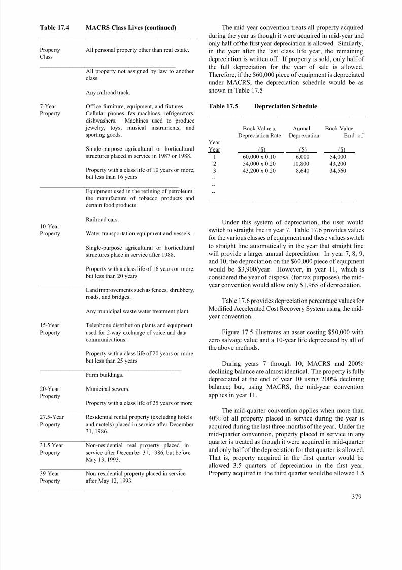
Table 17.5 Depreciation Schedule
________________________________________________
Book Value x Annual Book Value
Depreciation Rate Depreciation End of
Year
Year ($) ($) ($)
1 60,000 x 0.10 6,000 54,000
2 54,000 x 0.20 10,800 43,200
3 43,200 x 0.20 8,640 34,560
--
--
--
__________________________________________________
Under this system of depreciation, the user would
switch to straight line in year 7. Table 17.6 provides values
for the various classes of equipment and these values switch
to straight line automatically in the year that straight line
will provide a larger annual depreciation. In year 7, 8, 9,
and 10, the depreciation on the $60,000 piece of equipment
would be $3,900/year. However, in year 11, which is
considered the year of disposal (for tax purposes), the mid-
year convention would allow only $1,965 of depreciation.
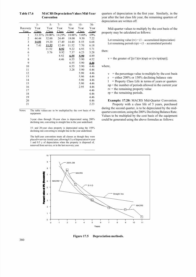
Table 17.6 provides depreciation percentage values for Modified Accelerated Cost Recovery System using the mid-
year convention.
Figure 17.5 illustrates an asset costing $50,000 with
zero salvage value and a 10-year life depreciated by all of
the above methods.
During years 7 through 10, MACRS and 200%
declining balance are almost identical. The property is fully
depreciated at the end of year 10 using 200% declining
balance; but, using MACRS, the mid-year convention
applies in year 11.
The mid-quarter convention applies when more than
40% of all property placed in service during the year is
acquired during the last three months of the year. Under the
mid-quarter convention, property placed in service in any
quarter is treated as though it were acquired in mid-quarter
and only half of the depreciation for that quarter is allowed.
That is, property acquired in the first quarter would be
allowed 3.5 quarters of depreciation in the first year.
Property acquired in the third quarter would be allowed 1.5
379
8/12/2019 Costing & Analysis for Engineering
http://slidepdf.com/reader/full/costing-analysis-for-engineering 22/48
Years
0 1 2
200% DB
4 5 6 7 8 9 10 11
0
1
2
3
4
5
6
8
7
9
10
3
MACRS
S-Y-D
Straight line
MACRS
MACRS
Table 17.6 MACRS Depreciation Values Mid-Year
Convention
________________________________________________ 3- 5- 7- 10- 15- 20-
Recovery Year Year Year Year Year Year
Year Class Class Class Class Class Class
1 33.33% 20.00% 14.29% 10.00% 5.00% 3.75%
2 44.44 32.00 24.49 18.00 9.50 7.22
3 14.81 19.20 17.49 14.40 8 .55 6.68
4 7.41 11.52 12.49 11.52 7.70 6.18
5 11.52 8.92 9.22 6.93 5.71 6 5.76 8.92 7.37 6.23 5.28
7 8.92 6.55 5.90 4.89
8 4.46 6.55 5.90 4.52
9 6.55 5.90 4.46
10 6.55 5.90 4.46
11 3.28 5.90 4.46
12 5.90 4.46
13 5.90 4.46
14 5.90 4.46
15 5.90 4.46
16 2.95 4.46
17 4.46
18 4.46
19 4.4620 4.46
21 2.23
__________________ Notes: The table values are to be multiplied by the cost basis of the
equipment.
3-year class through 10-year class is depreciated using 200%declining rate, converting to straight line in the year underlined.
15- and 20-year class property is depreciated using the 150%
declining rate converting to straight line in the year underlined.
The half-year convention treats all classes as though they were placed in service in mid-year, allowing 0.5 y of depreciation in year 1 and 0.5 y of depreciation when the property is disposed of,
removed from service, or in the last recovery year. ____________________________________________________
quarters of depreciation in the first year. Similarly, in the
year after the last class life year, the remaining quarters of
depreciation are written off.
Mid-quarter values to multiply by the cost basis of the
property may be calculated as follows:
Let remaining value (rv) = (1 - accumulated depreciation)
Let remaining periods (rp) = (1 - accumulated periods)
then:
v = the greater of [(r/1)(rv)(np) or (rv/rp)(np)].
where,
v = the percentage value to multiple by the cost basis
r = either 200% or 150% declining balance rate
l = Property Class Life in terms of years or quarters
np = the number of periods allowed in the current year
rv = the remaining property value
rp = the remaining periods.
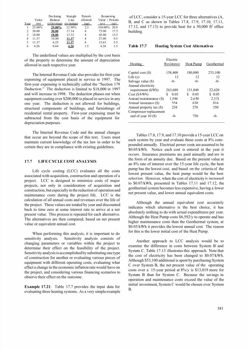
Example: 17.20: MACRS Mid-Quarter Convention.
Property with a class life of 5 years, purchased
during the second quarter, is to be depreciated by the mid-
quarter convention, using the 200% Declining Balance Rate.
Values to be multipled by the cost basis of the equipment
could be generated using the above formulas as follows:
Figure 17.5 Depreciation methods.
380
8/12/2019 Costing & Analysis for Engineering
http://slidepdf.com/reader/full/costing-analysis-for-engineering 23/48
Declining Straight Periods Remaining Value Balance Line Allowed Value | Periods
Year (m) (r/l)(rv)(np) (rv/rp)(np) (np) (rv) (rp)
1 25.00% 25.00% 12.50% 2.5 100.00% 20.0
2 30.00 30.00 17.14 4 75.00 17.5
3 18.00 18.00 13.33 4 45.00 13.5
4 11.37 10.80 11.37 4 27.00 9.5
5 11.37 6.25 11.37 4 15.63 5.5
6 4.26 0.64 4.26 1.5 4.26 1.5
The underlined values are multiplied by the cost basis
of the property to determine the amount of depreciationallowed in each respective year.
The Internal Revenue Code also provides for first-year
expensing of equipment placed in service in 1997. The
first-year expensing is technically called the “Section 179
Deduction.” The deduction is limited to $18,000 in 1997
and will increase in 1998. The deduction phases out when
equipment costing over $200,000 is placed in service in any
one year. The deduction is not allowed for buildings,
structural components of buildings, and furnishings of
residential rental property. First-year expensing must be
subtracted from the cost basis of the equipment for
depreciation purposes.
The Internal Revenue Code and the annual changes
that occur are beyond the scope of this text. Users must
maintain current knowledge of the tax law in order to be
certain they are in compliance with existing guidelines.
17.7 LIFE CYCLE COST ANALYSIS
Life cycle costing (LCC) evaluates all the costs
associated with acquisition, construction and operation of a
project. LCC is designed to minimize costs of major
projects, not only in consideration of acquisition andconstruction, but especially in the reduction of operation and
maintenance costs during the project life. LCC is the
calculation of all annual costs and revenues over the life of
the project. These values are totaled by year and discounted
back to time zero at some interest rate to arrive at a net
present value. This process is repeated for each alternative.
The alternatives are then compared, based on net present
value or equivalent annual cost.
When performing this analysis, it is important to do
sensitivity analysis. Sensitivity analysis consists of
changing parameters or variables within the project todetermine their effect on the feasibility of the project.
Sensitivity analysis is accomplished by substituting one type
of construction for another or evaluating various pieces of
equipment with different operating costs, evaluating what
effect a change in the economic inflation rate would have on
the project, and considering various financing scenarios to
observe their effect on the outcome.
Example 17.21: Table 17.7 provides the input data for
evaluating three heating systems. As a very simple example
of LCC, consider a 15-year LCC for three alternatives (A,
B, and C as shown in Tables 17.8, 17.9, 17.10, 17.11,
17.12, and 17.13) to provide heat for a 30,000 ft2 office
building.
Table 17.7 Heating System Cost Alternatives
________________________________________________
Electric Heating Resistance Heat Pump Geothermal
Capital cost ($) 158,400 180,000 233,100
Life (y) 12 12 12
Salvage value ($) -0- -0- -0-
Annual electricity
requirement (kWh) 263,680 131,840 22,620
Cost ($/kWh) $ 0.05 $ 0.05 $ 0.05
Annual maintenance ($) 1,584 2,650 2,331
Annual insurance ($) 554 630 816
Annual property tax ($) 238 270 350
Compressor replacement
end of year 10 ($) -0- 750 -0-
________________________________________________
Tables 17.8, 17.9, and 17.10 provide a 15-year LCC on
each system by year and evaluate these costs at 8% com-
pounded annually. Electrical power costs are assumed to be
$0.05/kWh. Notice each cost is entered in the year it
occurs. Insurance premiums are paid annually and are in
the form of an annuity due. Based on the present value at
an 8% rate of interest over the 15-year life cycle, the heat
pump has the lowest cost, and based on the criteria of the
lowest present value, the heat pump would be the best
selection. However, when the cost of electricity is increased
to $0.07/kWh, presented in Tables 17.11 and 17.12, thegeothermal system becomes less expensive, having a lower
net present value, and lower annual equivalent costs.
Although the annual equivalent cost accurately
indicates which alternative is the best choice, it has
absolutely nothing to do with actual expenditures per year.
Although the Heat Pump costs $6,592/y to operate and has
higher maintenance costs than the Geothermal system, at
$0.05/kWh it provides the lowest annual cost. The reason
for this is the lower initial cost of the Heat Pump.
Another approach to LCC analysis would be to
examine the difference in costs between System B andSystem C. Table 17.13 illustrates this approach. Note that
the cost of electricity has been changed to $0.07/kWh.
Although $53,100 additional is spent by purchasing System
C over System B, the net present value of the operating
costs over a 15-year period at 8%/y is $13,019 more for
System B than for System C. Because the savings in
operation and maintenance costs exceed the value of the
initial investment, System C would be chosen over System
B.
381
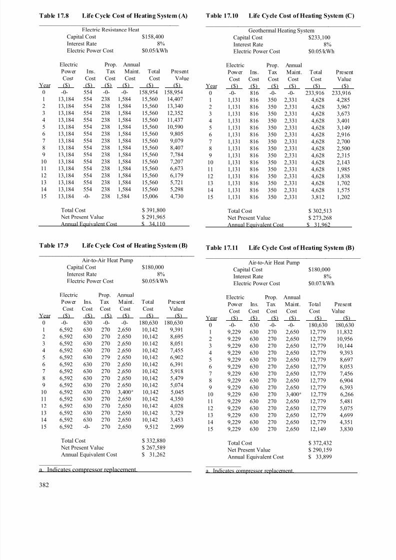
8/12/2019 Costing & Analysis for Engineering
http://slidepdf.com/reader/full/costing-analysis-for-engineering 24/48
Table 17.8 Life Cycle Cost of Heating System (A) ________________________________________________
Electric Resistance Heat
Capital Cost $158,400
Interest Rate 8%
Electric Power Cost $0.05/kWh
Electric Prop. Annual
Power Ins. Tax Maint. Total Present
Cost Cost Cost Cost Cost Value
Year ($) ($) ($) ($) ($) ($)
0 -0- 554 -0- -0- 158,954 158,954
1 13,184 554 238 1,584 15,560 14,407 2 13,184 554 238 1,584 15,560 13,340
3 13,184 554 238 1,584 15,560 12,352
4 13,184 554 238 1,584 15,560 11,437
5 13,184 554 238 1,584 15,560 10,590
6 13,184 554 238 1,584 15,560 9,805
7 13,184 554 238 1,584 15,560 9,079
8 13,184 554 238 1,584 15,560 8,407
9 13,184 554 238 1,584 15,560 7,784
10 13,184 554 238 1,584 15,560 7,207
11 13,184 554 238 1,584 15,560 6,673
12 13,184 554 238 1,584 15,560 6,179
13 13,184 554 238 1,584 15,560 5,721
14 13,184 554 238 1,584 15,560 5,298
15 13,184 -0- 238 1,584 15,006 4,730
Total Cost $ 391,800
Net Present Value $ 291,965
Annual Equivalent Cost $ 34,110
Table 17.9 Life Cycle Cost of Heating System (B)
________________________________________________ Air-to-Air Heat Pump
Capital Cost $180,000
Interest Rate 8%
Electric Power Cost $0.05/kWh
Electric Prop. Annual Power Ins. Tax Maint. Total Present
Cost Cost Cost Cost Cost Value
Year ($) ($) ($) ($) ($) ($)
0 -0- 630 -0- -0- 180,630 180,630
1 6,592 630 270 2,650 10,142 9,391
2 6,592 630 270 2 ,650 10,142 8,695
3 6,592 630 270 2 ,650 10.142 8,051
4 6,592 630 270 2 ,650 10,142 7,455
5 6,592 630 279 2 ,650 10,142 6,902
6 6,592 630 270 2 ,650 10,142 6,391
7 6,592 630 270 2 ,650 10,142 5,918
8 6,592 630 270 2 ,650 10,142 5,479
9 6,592 630 270 2 ,650 10,142 5,074
10 6,592 630 270 3,400a
10,142 5,045 11 6,592 630 270 2,650 10,142 4,350
12 6,592 630 270 2,650 10,142 4,028
13 6,592 630 270 2,650 10,142 3,729
14 6,592 630 270 2,650 10,142 3,453
15 6,592 -0- 270 2,650 9,512 2,999
Total Cost $ 332,880
Net Present Value $ 267,589
Annual Equivalent Cost $ 31,262
__________
a. Indicates compressor replacement.
382
Table 17.10 Life Cycle Cost of Heating System (C)
________________________________________________ Geothermal Heating System
Capital Cost $233,100
Interest Rate 8%
Electric Power Cost $0.05/kWh
Electric Prop. Annual
Power Ins. Tax Maint. Total Present
Cost Cost Cost Cost Cost Value
Year ($) ($) ($) ($) ($) ($)
0 -0- 816 -0- -0- 233,916 233,916
1 1,131 816 350 2,331 4,628 4,285 2 1,131 816 350 2,331 4,628 3,967
3 1,131 816 350 2,331 4,628 3,673
4 1,131 816 350 2,331 4,628 3,401
5 1,131 816 350 2,331 4,628 3,149
6 1,131 816 350 2,331 4,628 2,916
7 1,131 816 350 2,331 4,628 2,700
8 1,131 816 350 2,331 4,628 2,500
9 1,131 816 350 2,331 4,628 2,315
10 1,131 816 350 2,331 4,628 2,143
11 1,131 816 350 2,331 4,628 1,985
12 1,131 816 350 2,331 4,628 1,838
13 1,131 816 350 2,331 4,628 1,702
14 1,131 816 350 2,331 4,628 1,575
15 1,131 816 350 2,331 3,812 1,202
Total Cost $ 302,513
Net Present Value $ 273,268
Annual Equivalent Cost $ 31,962
Table 17.11 Life Cycle Cost of Heating System (B)
________________________________________________ Air-to-Air Heat Pump
Capital Cost $180,000
Interest Rate 8%
Electric Power Cost $0.07/kWh
Electric Prop. Annual
Power Ins. Tax Maint. Total Present
Cost Cost Cost Cost Cost Value
Year ($) ($) ($) ($) ($) ($)
0 -0- 630 -0- -0- 180,630 180,630
1 9,229 630 270 2,650 12,779 11,832
2 9.229 630 270 2,650 12,779 10,956
3 9,229 630 270 2,650 12,779 10,144
4 9,229 630 270 2,650 12,779 9,393
5 9,229 630 270 2,650 12,779 8,697
6 9,229 630 270 2,650 12,779 8,053
7 9,229 630 270 2,650 12,779 7,456
8 9,229 630 270 2,650 12,779 6,904
9 9,229 630 270 2,650 12,779 6,393
10 9,229 630 270 3,400a 12,779 6,266 11 9,229 630 270 2,650 12,779 5,481
12 9,229 630 270 2,650 12,779 5,075
13 9,229 630 270 2,650 12,779 4,699
14 9,229 630 270 2,650 12,779 4,351
15 9,229 630 270 2,650 12,149 3,830
Total Cost $ 372,432
Net Present Value $ 290,159
Annual Equivalent Cost $ 33,899
____________
a. Indicates compressor replacement.
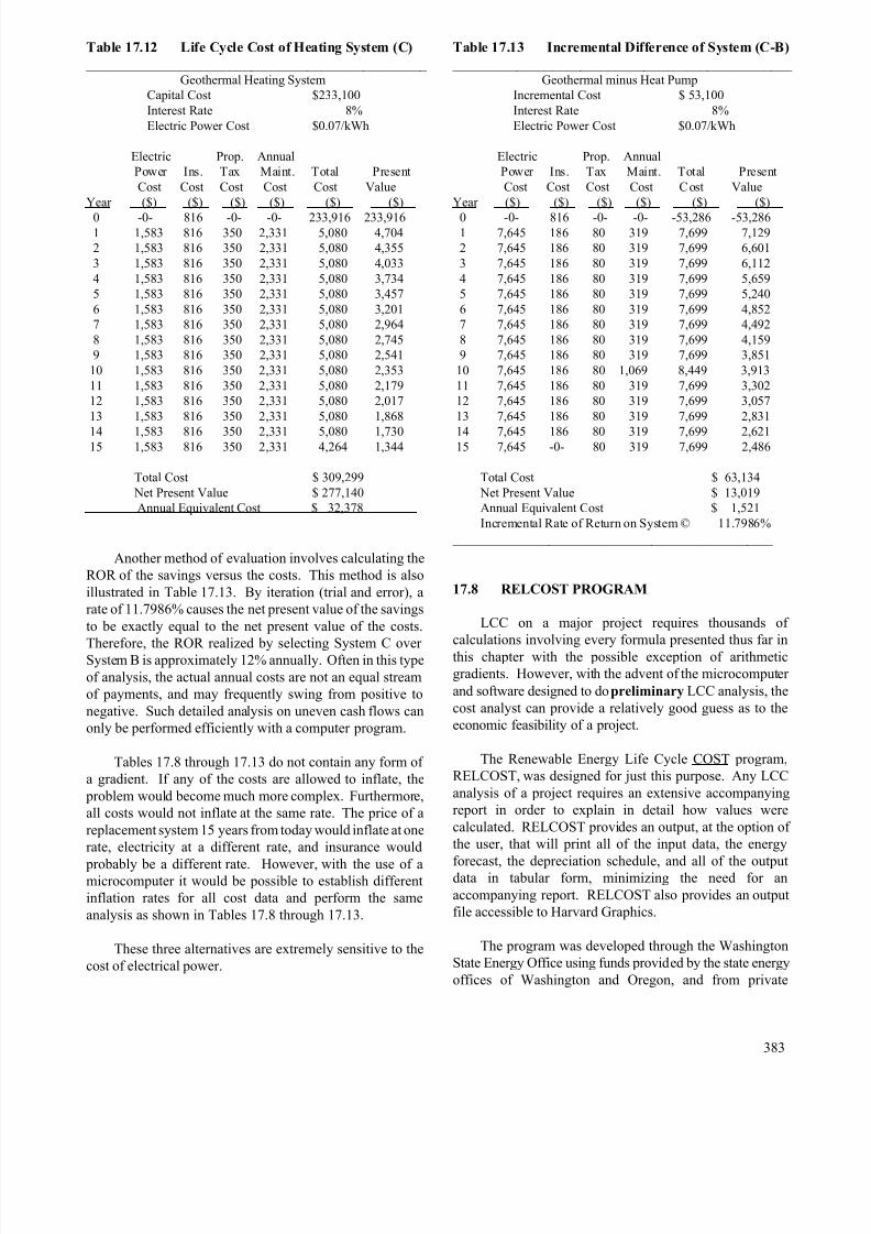
8/12/2019 Costing & Analysis for Engineering
http://slidepdf.com/reader/full/costing-analysis-for-engineering 25/48
Table 17.12 Life Cycle Cost of Heating System (C)
________________________________________________ Geothermal Heating System
Capital Cost $233,100
Interest Rate 8%
Electric Power Cost $0.07/kWh
Electric Prop. Annual
Power Ins. Tax Maint. Total Present
Cost Cost Cost Cost Cost Value
Year ($) ($) ($) ($) ($) ($)
0 -0- 816 -0- -0- 233,916 233,916 1 1,583 816 350 2,331 5,080 4,704
2 1,583 816 350 2,331 5,080 4,355
3 1,583 816 350 2,331 5,080 4,033
4 1,583 816 350 2,331 5,080 3,734
5 1,583 816 350 2,331 5,080 3,457
6 1,583 816 350 2,331 5,080 3,201
7 1,583 816 350 2,331 5,080 2,964
8 1,583 816 350 2,331 5,080 2,745
9 1,583 816 350 2,331 5,080 2,541
10 1,583 816 350 2,331 5,080 2,353
11 1,583 816 350 2,331 5,080 2,179
12 1,583 816 350 2,331 5,080 2,017
13 1,583 816 350 2,331 5,080 1,868
14 1,583 816 350 2,331 5,080 1,730 15 1,583 816 350 2,331 4,264 1,344
Total Cost $ 309,299
Net Present Value $ 277,140
Annual Equivalent Cost $ 32,378
Another method of evaluation involves calculating the
ROR of the savings versus the costs. This method is also
illustrated in Table 17.13. By iteration (trial and error), a
rate of 11.7986% causes the net present value of the savings
to be exactly equal to the net present value of the costs.
Therefore, the ROR realized by selecting System C over System B is approximately 12% annually. Often in this type
of analysis, the actual annual costs are not an equal stream
of payments, and may frequently swing from positive to
negative. Such detailed analysis on uneven cash flows can
only be performed efficiently with a computer program.
Tables 17.8 through 17.13 do not contain any form of
a gradient. If any of the costs are allowed to inflate, the
problem would become much more complex. Furthermore,
all costs would not inflate at the same rate. The price of a
replacement system 15 years from today would inflate at one
rate, electricity at a different rate, and insurance would
probably be a different rate. However, with the use of amicrocomputer it would be possible to establish different
inflation rates for all cost data and perform the same
analysis as shown in Tables 17.8 through 17.13.
These three alternatives are extremely sensitive to the
cost of electrical power.
Table 17.13 Incremental Difference of System (C-B)
________________________________________________ Geothermal minus Heat Pump
Incremental Cost $ 53,100
Interest Rate 8%
Electric Power Cost $0.07/kWh
Electric Prop. Annual
Power Ins. Tax Maint. Total Present
Cost Cost Cost Cost Cost Value
Year ($) ($) ($) ($) ($) ($)
0 -0- 816 -0- -0- -53,286 -53,286 1 7,645 186 80 319 7,699 7,129
2 7,645 186 80 319 7,699 6,601
3 7,645 186 80 319 7,699 6,112
4 7,645 186 80 319 7,699 5,659
5 7,645 186 80 319 7,699 5,240
6 7,645 186 80 319 7,699 4,852
7 7,645 186 80 319 7,699 4,492
8 7,645 186 80 319 7,699 4,159
9 7,645 186 80 319 7,699 3,851
10 7,645 186 80 1,069 8,449 3,913
11 7,645 186 80 319 7,699 3,302
12 7,645 186 80 319 7,699 3,057
13 7,645 186 80 319 7,699 2,831
14 7,645 186 80 319 7,699 2,621 15 7,645 -0- 80 319 7,699 2,486
Total Cost $ 63,134
Net Present Value $ 13,019
Annual Equivalent Cost $ 1,521
Incremental Rate of Return on System © 11.7986%
__________________________________________________
17.8 RELCOST PROGRAM
LCC on a major project requires thousands of
calculations involving every formula presented thus far in
this chapter with the possible exception of arithmetic
gradients. However, with the advent of the microcomputer
and software designed to do preliminary LCC analysis, the
cost analyst can provide a relatively good guess as to the
economic feasibility of a project.
The Renewable Energy Life Cycle COST program,
RELCOST, was designed for just this purpose. Any LCC
analysis of a project requires an extensive accompanying
report in order to explain in detail how values were
calculated. RELCOST provides an output, at the option of
the user, that will print all of the input data, the energy
forecast, the depreciation schedule, and all of the outputdata in tabular form, minimizing the need for an
accompanying report. RELCOST also provides an output
file accessible to Harvard Graphics.
The program was developed through the Washington
State Energy Office using funds provided by the state energy
offices of Washington and Oregon, and from private
383
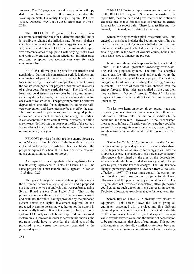
8/12/2019 Costing & Analysis for Engineering
http://slidepdf.com/reader/full/costing-analysis-for-engineering 26/48
sources. The 150 page user manual is supplied on a floppy
disk. To obtain copies of this program, contact the
Washington State University Energy Program, PO Box
43165, Olympia, WA 98504-3165, telephone: 360-956-
2016.
The RELCOST Program, Release 2.1, can
accommodate inflation rates for 13 different energies, and it
is possible to change the inflation rate for each of these
energies every year throughout an energy forecast of up to
30 years. In addition, RELCOST will accommodate up tofive different classes of equipment with varying useful lives
and with different depreciation schedules. Inflation rates
regarding equipment replacement can vary for each
equipment class.
RELCOST allows up to 5 years for construction and
acquisition. During this construction period, it allows any
combination of project financing to include bonds, bank
loans, and equity. It also allows capital investment during
the construction period for project funds that are in excess
of project costs for any particular year. The life of bank
loans and bond issues can vary year by year, and interest
rates may differ for bonds, bank loans, and investments for
each year of construction. The program permits 12 different
depreciation schedules for equipment, including the half-
year convention, and these rates may be altered by the user.
The program makes provisions for percentage depletion
allowances, investment tax credits, and energy tax credits.
It can accept up to three annual revenue streams, inflating
at some user-defined rate per year over the life of the project.
It also allows for a growth rate in the number of customers
on-line in any given year.
RELCOST provides for four resident energy forecasts,
up to 30 years in length. Once all the input data has beencollected, and energy forecasts have been established, the
program requires less than 30 minutes to enter the data and
do the calculations for a major project.
A complete run on a hypothetical heating district for a
taxable entity is provided in Tables 17.14 thru 17.22. The
same project for a non-taxable entity appears in Tables
17.23 thru 17.29.
The typical life-cycle cost input data supplied considers
the difference between an existing system and a proposed
system; the same type of analysis that was performed using
System B and System C in Table 17.13. That is, the program considers the initial cost of the proposed system
and evaluates the annual savings provided by the proposed
system versus the capital investment required for the
proposed system to determine whether or not the system is
economically feasible. It is not necessary to have a present
system. LCC analysis could be accomplished on a proposed
system only. However, in order to perform this analysis, the
program would have to consider the initial cost of the
proposed system versus the revenues generated by the
proposed system.
384
Table 17.14 illustrates input screen one, two, and three
of the RELCOST Program. Screen one consists of the
report title, location, date, and gives the user the option of
choosing one of four forecast files or creating an energy
forecast for this report only. These forecast files must be
created, maintained, and updated by the user.
Screen two begins with capital investment data. Data
entered on this sheet includes the beginning year of invest-
ment, construction period, economic inflation rate, discount
rate or cost of capital selected for the project and allfinancing data in the form of owner's equity, bonds, and
bank loans used to finance the project.
Input screen three, which appears in the lower third of
Table 17.14, includes all present costs of energy for the exis-
ting and the proposed system. The first five energies:
natural gas, fuel oil, propane, coal, and electricity, are the
conventional fuels supplied for every project. The next five
energies included under the heading Other Energy" are user
selectable. The titles of these fuels are obtained from the
energy forecast. If no titles are supplied by the user, then
they are listed as "Other 1" through "Other 5." The user
may elect to use any one or all of these fuels in the project
under study.
The last two items on screen three: property tax and
insurance, and operation and maintenance, have their own
independent inflation rates that are not in addition to the
economic inflation rate. However, if the user wanted
these rates to inflate differently year by year, they could be
entered on an energy forecast as an energy, properly titled,
and these two items could be omitted at the bottom of screen
three.
Screen four Table 17.15 presents energy sales for boththe present and proposed systems. This screen also allows
percentages depletion allowance for energy sales under the
proposed system. The amount of the percentage depletion
allowance is determined by the user on the depreciation
schedule under depletion, and if necessary, could change
year by year, or as the tax code changes. The 1986 tax code
changed percentage depletion allowance from 20 to 22%,
effective in 1987. The user must consult the current tax
code to determine those energies eligible for depletion
allowance and the percent of depletion allowance. The
program does not provide cost depletion, although the user
could calculate such depletion in the depreciation section.
Depletion allowances are only available for taxable entities.
Screen five on Table 17.15 presents five classes of
equipment. This screen allows the user to group all
equipment associated with a project into five different
classes depending upon economic life (the actual usable life
of the equipment), taxable life, actual expected salvage
value, taxable salvage value, and the method of depreciation
to be applied against that class of equipment. This portion
of the input section also allows inflation rates for subsequent
purchases of equipment and inflation rates for actual salvage
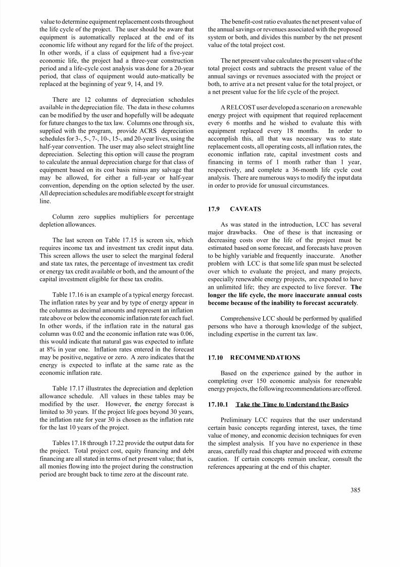
8/12/2019 Costing & Analysis for Engineering
http://slidepdf.com/reader/full/costing-analysis-for-engineering 27/48
value to determine equipment replacement costs throughout
the life cycle of the project. The user should be aware that
equipment is automatically replaced at the end of its
economic life without any regard for the life of the project.
In other words, if a class of equipment had a five-year
economic life, the project had a three-year construction
period and a life-cycle cost analysis was done for a 20-year
period, that class of equipment would auto-matically be
replaced at the beginning of year 9, 14, and 19.
There are 12 columns of depreciation schedulesavailable in the depreciation file. The data in these columns
can be modified by the user and hopefully will be adequate
for future changes to the tax law. Columns one through six,
supplied with the program, provide ACRS depreciation
schedules for 3-, 5-, 7-, 10-, 15-, and 20-year lives, using the
half-year convention. The user may also select straight line
depreciation. Selecting this option will cause the program
to calculate the annual depreciation charge for that class of
equipment based on its cost basis minus any salvage that
may be allowed, for either a full-year or half-year
convention, depending on the option selected by the user.
All depreciation schedules are modifiable except for straight
line.
Column zero supplies multipliers for percentage
depletion allowances.
The last screen on Table 17.15 is screen six, which
requires income tax and investment tax credit input data.
This screen allows the user to select the marginal federal
and state tax rates, the percentage of investment tax credit
or energy tax credit available or both, and the amount of the
capital investment eligible for these tax credits.
Table 17.16 is an example of a typical energy forecast.The inflation rates by year and by type of energy appear in
the columns as decimal amounts and represent an inflation
rate above or below the economic inflation rate for each fuel.
In other words, if the inflation rate in the natural gas
column was 0.02 and the economic inflation rate was 0.06,
this would indicate that natural gas was expected to inflate
at 8% in year one. Inflation rates entered in the forecast
may be positive, negative or zero. A zero indicates that the
energy is expected to inflate at the same rate as the
economic inflation rate.
Table 17.17 illustrates the depreciation and depletion
allowance schedule. All values in these tables may bemodified by the user. However, the energy forecast is
limited to 30 years. If the project life goes beyond 30 years,
the inflation rate for year 30 is chosen as the inflation rate
for the last 10 years of the project.
Tables 17.18 through 17.22 provide the output data for
the project. Total project cost, equity financing and debt
financing are all stated in terms of net present value; that is,
all monies flowing into the project during the construction
period are brought back to time zero at the discount rate.
The benefit-cost ratio evaluates the net present value of
the annual savings or revenues associated with the proposed
system or both, and divides this number by the net present
value of the total project cost.
The net present value calculates the present value of the
total project costs and subtracts the present value of the
annual savings or revenues associated with the project or
both, to arrive at a net present value for the total project, or
a net present value for the life cycle of the project.
A RELCOST user developed a scenario on a renewable
energy project with equipment that required replacement
every 6 months and he wished to evaluate this with
equipment replaced every 18 months. In order to
accomplish this, all that was necessary was to state
replacement costs, all operating costs, all inflation rates, the
economic inflation rate, capital investment costs and
financing in terms of 1 month rather than 1 year,
respectively, and complete a 36-month life cycle cost
analysis. There are numerous ways to modify the input data
in order to provide for unusual circumstances.
17.9 CAVEATS
As was stated in the introduction, LCC has several
major drawbacks. One of these is that increasing or
decreasing costs over the life of the project must be
estimated based on some forecast, and forecasts have proven
to be highly variable and frequently inaccurate. Another
problem with LCC is that some life span must be selected
over which to evaluate the project, and many projects,
especially renewable energy projects, are expected to have
an unlimited life; they are expected to live forever. The
longer the life cycle, the more inaccurate annual costsbecome because of the inability to forecast accurately.
Comprehensive LCC should be performed by qualified
persons who have a thorough knowledge of the subject,
including expertise in the current tax law.
17.10 RECOMMENDATIONS
Based on the experience gained by the author in
completing over 150 economic analysis for renewable
energy projects, the following recommendations are offered.
17.10.1 Take the Time to Understand the Basics
Preliminary LCC requires that the user understand
certain basic concepts regarding interest, taxes, the time
value of money, and economic decision techniques for even
the simplest analysis. If you have no experience in these
areas, carefully read this chapter and proceed with extreme
caution. If certain concepts remain unclear, consult the
references appearing at the end of this chapter.
385
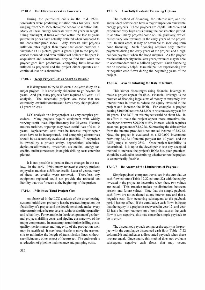
8/12/2019 Costing & Analysis for Engineering
http://slidepdf.com/reader/full/costing-analysis-for-engineering 28/48
17.10.2 Use Ultraconservative Forecasts
During the petroleum crisis in the mid 1970s,
forecasters were predicting inflation rates for fossil fuels
ranging from 5 to 15% above the economic inflation rate.
Many of these energy forecasts were 20 years in length.
Using hindsight, it turns out that within the last 10 years
petroleum prices have actually deflated when compared to
the consumer price index. Any forecast that projects
inflation rates higher than those that occur provides a
favorable LCC picture, gives a green light to the project,causes thousands and even millions of dollars to be spent in
acquisition and construction, only to find that when the
project goes into production, competing fuels have not
inflated as projected and the project either operates at a
continual loss or is abandoned.
17.10.3 Keep Project Life as Short as Possible
It is dangerous to try to do even a 20-year study on a
major project. It is absolutely ridiculous to go beyond 20
years. And yet, many projects have required 50-year LCC
analysis. The successful projects are those that use
extremely low inflation rates and have a very short payback (4 years or less).
LCC analysis on a large project is a very complex pro-
cedure. Many projects require equipment with widely
varying useful lives. Pipe lines may last 25 years. Electric
motors, turbines, or pumps may have useful lives of 5 to 10
years. Replacement costs must be forecast, major repair
costs have to be incorporated, and competing alternatives
should be as accurately evaluated as possible. If the project
is owned by a private entity, depreciation schedules,
depletion allowances, investment tax credits, energy tax
credits, and in some cases, intangible drilling costs enter the picture.
It is not possible to predict future changes in the tax
law. In the early 1980s, many renewable energy projects
enjoyed as much as a 55% tax credit. Later (5 years), many
of these tax credits were removed. Therefore, any
equipment replaced could not provide the reduced tax
liability that was forecast at the beginning of the project.
17.10.4 Minimize Total Project Cost
As observed in the LCC analysis of the three heating
systems, initial cost probably has the greatest impact on thefeasibility of a project and the developer should make every
effort to minimize the project cost without sacrificing quality
and reliability. For example, in the development of geother-
mal projects, drilling costs, and pipeline costs are two of the
major components. In an attempt to minimize drilling costs,
quality, performance and longevity of the production well
may be sacrificed. It may be advisable to move the user on-
site to minimize the length of transmission lines without
sacrificing any other aspect of the project. The end result is
a reduction of pipeline maintenance and pumping costs.
386
17.10.5 Carefully Evaluate Financing Options
The method of financing, the interest rate, and the
annual debt service can have a major impact on renewable
energy projects. These projects are capital intensive and
experience very high costs during the construction period.
In addition, many projects come on-line gradually, which
causes very low revenues in the early years of the project
life. In such cases, it may be advisable to seek long-term
bond financing. Such financing requires only interest
payments during the early years of the project, and a high balloon payment when the bond matures. As the project
reaches full capacity in the later years, revenues may be able
to accommodate such a balloon payment. Such financing
can be especially helpful to municipalities experiencing low
or negative cash flows during the beginning years of the
project.
17.10.6 Avoid Distorting the Rate of Return
This author discourages using financial leverage to
make a project appear feasible. Financial leverage is the
practice of financing large sums of money at extremely low
interest rates in order to reduce the equity invested in the project and increase the ROR. For example, a project
costing $100,000 returns $15,000 in revenues every year for
10 years. The ROR on this project would be about 8%. In
an effort to make the project appear more attractive, the
developer borrows $90,000 at 6% interest, which requires
an annual payment of $12,228. Subtracting the debt service
from the income provides a net annual income of $2,772.
Now, the project is evaluated as a $10,000 investment
providing $2,772 of income per year for 10 years and the
ROR jumps to nearly 25%. Once project feasibility is
determined, it is up to the developer to use any accepted
method to increase the project's ROR; but, such practicesshould be avoided in determining whether or not the project
is economically feasible.
17.10.7 Be Aware of the Limitations of Payback
Simple payback compares the values in the cumulative
cash flow column (Table 17.22 column 22) with the equity
invested in the project to determine when these two values
are equal. This practice makes no distinction between
present and future values. Note that the simple payback
cash flows are not evaluated at any interest rate and that a
negative cash flow occurring subsequent to the payback
period has no effect. If the cumulative cash flows indicatethat the equity in a project is recovered in year 12, and year
13 has a balloon payment on a bond that causes the cash
flow to turn negative, this may cause the simple payback to
be in error.
The discounted payback compares the equity in the pro-
ject with the cumulative discounted cash flow (Table 17.22
column 24) and indicates a discounted payback when these
two are equal. Once again, this method does not evaluate
subsequent negative cash flows that may occur.
8/12/2019 Costing & Analysis for Engineering
http://slidepdf.com/reader/full/costing-analysis-for-engineering 29/48
Nonetheless, it is a more accurate measure of payback
because the accumulated cash flows are discounted at the
discount rate stated in the input section.
The reason the simple and discounted payback periods
are evaluated in this manner is because it is the accepted
calculation method in the industry. Because these values
may be in error, the program RELCOST also evaluates cash
flows beyond these payback periods and prints a warning in
the output section if negative cash flows occur beyond the
payback period.
The LCC analysis is a very powerful tool. It can be
used to rank projects in the order of feasibility and to
determine which projects are most likely to be successful.
At best however, it is only an educated guess and the values
calculated should be treated only as rough estimates.
NOTE: See Glossary and References List at end of Chapter.
387
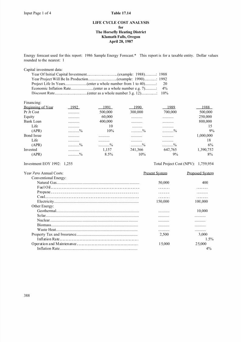
8/12/2019 Costing & Analysis for Engineering
http://slidepdf.com/reader/full/costing-analysis-for-engineering 30/48
Input Page 1 of 4 Table 17.14
LIFE CYCLE COST ANALYSIS
for
The Horsefly Heating District
Klamath Falls, Oregon
April 28, 1987
Energy forecast used for this report: 1986 Sample Energy Forecast.* This report is for a taxable entity. Dollar values
rounded to the nearest: 1
Capital investment data:
Year Of Initial Capital Investment...............................(example: 1988)...........: 1988
Year Project Will Be In Production.............................(example: 1990)............: 1992
Project Life In Years......................(enter a whole number from 1 to 40)...........: 20
Economic Inflation Rate.......................(enter as a whole number e.g. 7)...........: 4%
Discount Rate.................................(enter as a whole number 3.g. 12)...............: 10%
Financing:
Beginning of Year 1992 1991 1990 1989 1988
Pr Jt Cost ........... 500,000 300,000 700,000 500,000
Equity ........... 60,000 ........... ........... 250,000
Bank Loan ........... 400,000 ........... ........... 800,000
Life ........... 10 .......... ........... 15
(APR) ...........% 10% ...........% ...........% 9%
Bond Issue ........... ........... ........... ........... 1,000,000
Life ........... ........... ........... ........... 18
(APR) ...........% ...........% ...........% ...........% 6%
Invested ........... 1,157 241,366 642,765 1,390,752
(APR) ...........% 8.5% 10% 9% 8%
Investment EOY 1992: 1,255 Total Project Cost (NPV): 1,759,954
Year Zero Annual Costs: Present System Proposed System
Conventional Energy: Natural Gas........... ............... ................ ............... ............... .......... 50,000 400
Fuel Oil... ... .. ... .. ... ... .. ... .. ... ... .. ... .. ... ... .. ... .. ... ... .. ... ... .. ... .. ... ... .. ... .. .. . .. .. ... .. . . .. ... .. .. .
Propane....................................................................................... ........... ...........
Coal. ... .. ... .. ... .. .. ... .. ... .. ... .. .. ... .. ... .. ... .. .. ... .. ... .. ... .. .. ... .. ... .. ... .. .. ... .. .. . .. .. ... .. . . .. ... .. .. .
Electricity.................................................................................... 150,000 100,000
Other Energy:
Geothermal.................................................................................. ........... 10,000
Solar............................................................................................ ........... ...........
Nuclear. ............... ................ ............... ................ ............... ......... ........... ...........
Biomass...................................................................................... ........... ...........
Waste Heat................................................................................. ........... ...........
Property Tax and Insurance............................................................. 2,500 3,000
Inflation Rate... ... ... ... .. ... ... ... ... ... ... ... ... ... ... ... ... ... ... ... ... ... ... ... ... ... . 1.5%Operation and Maintenance.. ... ... ... .... ... ... .... ... ... ... .... ... ... ... .... ... ... ... . 15,000 25,000
Inflation Rate............................................................................. 4%
388
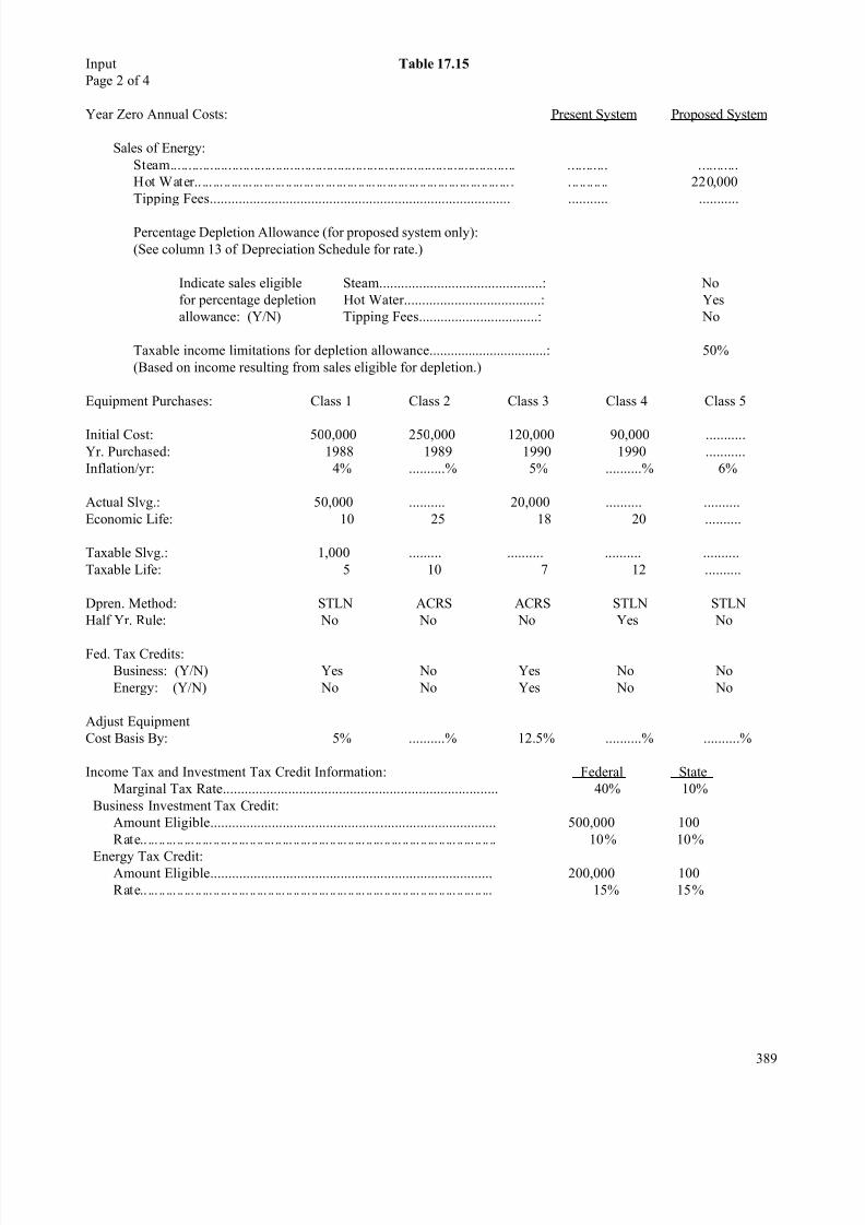
8/12/2019 Costing & Analysis for Engineering
http://slidepdf.com/reader/full/costing-analysis-for-engineering 31/48
Input Table 17.15
Page 2 of 4
Year Zero Annual Costs: Present System Proposed System
Sales of Energy:
Steam............................................................................................... ........... ...........
Hot Water.. ... ... .. ... ... ... ... ... .. ... ... ... ... ... ... .. ... ... ... ... ... .. ... ... ... ... ... .. ... ... . . .. .. .. .. .. 220,000
Tipping Fees................................................................................... ........... ...........
Percentage Depletion Allowance (for proposed system only):
(See column 13 of Depreciation Schedule for rate.)
Indicate sales eligible Steam.............................................: No
for percentage depletion Hot Water......................................: Yes
allowance: (Y/N) Tipping Fees.................................: No
Taxable income limitations for depletion allowance.................................: 50%
(Based on income resulting from sales eligible for depletion.)
Equipment Purchases: Class 1 Class 2 Class 3 Class 4 Class 5
Initial Cost: 500,000 250,000 120,000 90,000 ...........
Yr. Purchased: 1988 1989 1990 1990 ...........
Inflation/yr: 4% ..........% 5% ..........% 6%
Actual Slvg.: 50,000 .......... 20,000 .......... ..........
Economic Life: 10 25 18 20 ..........
Taxable Slvg.: 1,000 ......... .......... .......... ..........
Taxable Life: 5 10 7 12 ..........
Dpren. Method: STLN ACRS ACRS STLN STLN
Half Yr. Rule: No No No Yes No
Fed. Tax Credits:
Business: (Y/N) Yes No Yes No No
Energy: (Y/N) No No Yes No No
Adjust Equipment
Cost Basis By: 5% ..........% 12.5% ..........% ..........%
Income Tax and Investment Tax Credit Information: Federal State
Marginal Tax Rate............................................................................ 40% 10%
Business Investment Tax Credit:
Amount Eligible............................................................................... 500,000 100
Rate.. ... .. ... .. ... .. ... .. ... .. ... .. .. ... .. ... .. ... .. ... .. ... .. ... .. ... .. ... .. ... .. ... .. ... .. ... .. .. .. 10% 10%
Energy Tax Credit:Amount Eligible.............................................................................. 200,000 100
Rate.. ... .. ... .. ... .. ... .. ... .. ... .. ... .. ... .. .. ... .. ... .. ... .. ... .. ... .. ... .. ... .. ... .. ... .. ... .. ... 15% 15%
389
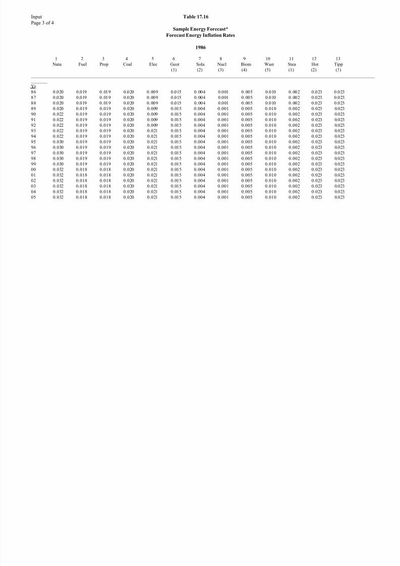
8/12/2019 Costing & Analysis for Engineering
http://slidepdf.com/reader/full/costing-analysis-for-engineering 32/48
Input Table 17.16
Page 3 of 4
Sample Energy Forecast*
Forecast Energy Inflation Rates
1986
1 2 3 4 5 6 7 8 9 10 11 12 13
Natu Fuel Prop Coal Elec Geot Sola Nucl Biom Wast Stea Hot Tipp
(1) (2) (3) (4) (5) (1) (2) (3)
____________________________________________________________________________________________________________________________________________________
_______
Yr
86 0.020 0.019 0.019 0.020 0.009 0.015 0.004 0.001 0.005 0.010 0.002 0.023 0.023
87 0.020 0.019 0.019 0.020 0.009 0.015 0.004 0.001 0.005 0.010 0.002 0.023 0.02388 0.020 0.019 0.019 0.020 0.009 0.015 0.004 0.001 0.005 0.010 0.002 0.023 0.023
89 0.020 0.019 0.019 0.020 0.009 0.015 0.004 0.001 0.005 0.010 0.002 0.023 0.023
90 0.022 0.019 0.019 0.020 0.009 0.015 0.004 0.001 0.005 0.010 0.002 0.023 0.023
91 0.022 0.019 0.019 0.020 0.009 0.015 0.004 0.001 0.005 0.010 0.002 0.023 0.023
92 0.022 0.019 0.019 0.020 0.009 0.015 0.004 0.001 0.005 0.010 0.002 0.023 0.023
93 0.022 0.019 0.019 0.020 0.021 0.015 0.004 0.001 0.005 0.010 0.002 0.023 0.023
94 0.022 0.019 0.019 0.020 0.021 0.015 0.004 0.001 0.005 0.010 0.002 0.023 0.023
95 0.030 0.019 0.019 0.020 0.021 0.015 0.004 0.001 0.005 0.010 0.002 0.023 0.023
96 0.030 0.019 0.019 0.020 0.021 0.015 0.004 0.001 0.005 0.010 0.002 0.023 0.023
97 0.030 0.019 0.019 0.020 0.021 0.015 0.004 0.001 0.005 0.010 0.002 0.023 0.023
98 0.030 0.019 0.019 0.020 0.021 0.015 0.004 0.001 0.005 0.010 0.002 0.023 0.023
99 0.030 0.019 0.019 0.020 0.021 0.015 0.004 0.001 0.005 0.010 0.002 0.023 0.023
00 0.032 0.018 0.018 0.020 0.021 0.015 0.004 0.001 0.005 0.010 0.002 0.023 0.023
01 0.032 0.018 0.018 0.020 0.021 0.015 0.004 0.001 0.005 0.010 0.002 0.023 0.023
02 0.032 0.018 0.018 0.020 0.021 0.015 0.004 0.001 0.005 0.010 0.002 0.023 0.023
03 0.032 0.018 0.018 0.020 0.021 0.015 0.004 0.001 0.005 0.010 0.002 0.023 0.023
04 0.032 0.018 0.018 0.020 0.021 0.015 0.004 0.001 0.005 0.010 0.002 0.023 0.023
05 0.032 0.018 0.018 0.020 0.021 0.015 0.004 0.001 0.005 0.010 0.002 0.023 0.023
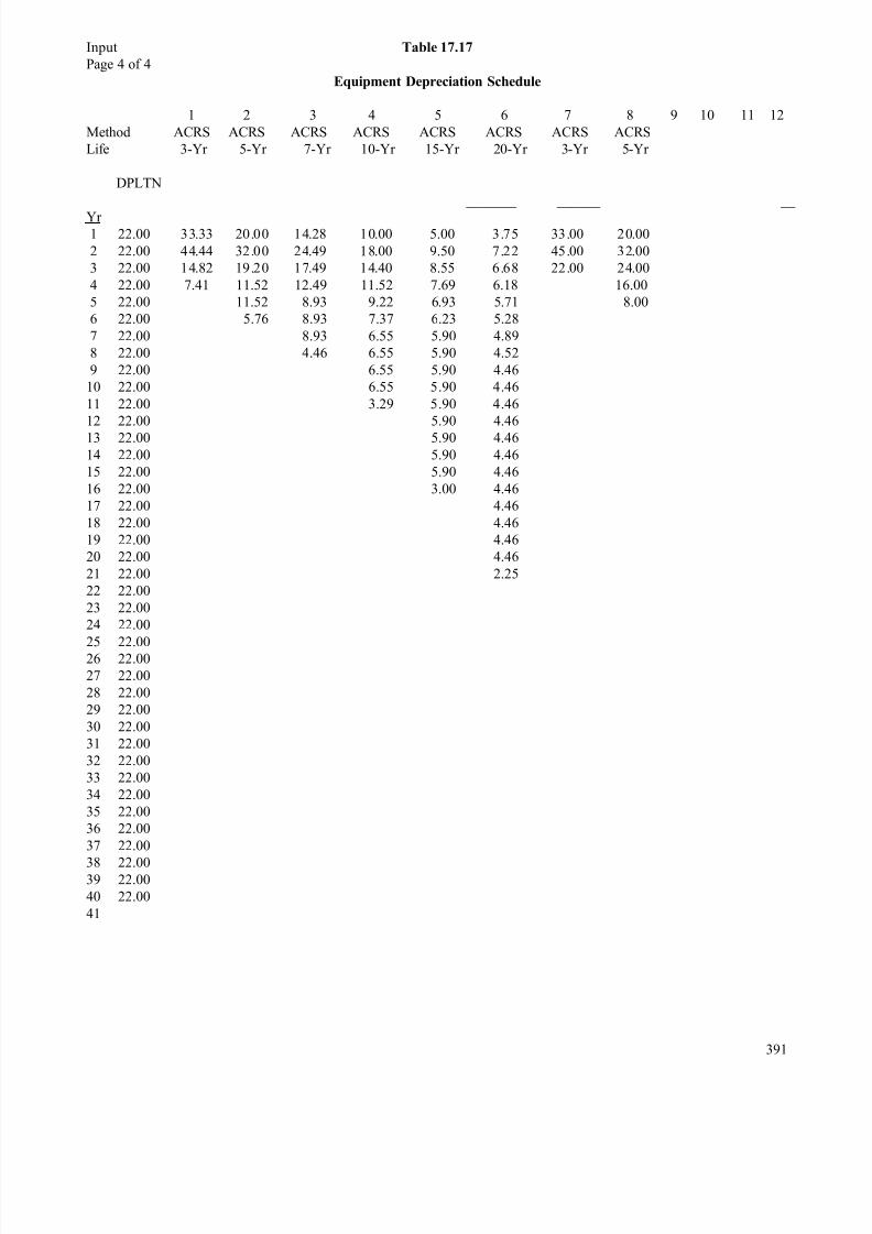
8/12/2019 Costing & Analysis for Engineering
http://slidepdf.com/reader/full/costing-analysis-for-engineering 33/48
Input Table 17.17
Page 4 of 4
Equipment Depreciation Schedule
1 2 3 4 5 6 7 8 9 10 11 12
Method ACRS ACRS ACRS ACRS ACRS ACRS ACRS ACRS
Life 3-Yr 5-Yr 7-Yr 10-Yr 15-Yr 20-Yr 3-Yr 5-Yr
DPLTN
____________________________________________________________________________________________________
Yr 1 22.00 33.33 20.00 14.28 10.00 5.00 3.75 33.00 20.00
2 22.00 44.44 32.00 24.49 18.00 9.50 7.22 45.00 32.00
3 22.00 14.82 19.20 17.49 14.40 8.55 6.68 22.00 24.00
4 22.00 7.41 11.52 12.49 11.52 7.69 6.18 16.00
5 22.00 11.52 8.93 9.22 6.93 5.71 8.00
6 22.00 5.76 8.93 7.37 6.23 5.28
7 22.00 8.93 6.55 5.90 4.89
8 22.00 4.46 6.55 5.90 4.52
9 22.00 6.55 5.90 4.46
10 22.00 6.55 5.90 4.46
11 22.00 3.29 5.90 4.46
12 22.00 5.90 4.46
13 22.00 5.90 4.46
14 22.00 5.90 4.46
15 22.00 5.90 4.46
16 22.00 3.00 4.46
17 22.00 4.46
18 22.00 4.46
19 22.00 4.46
20 22.00 4.46
21 22.00 2.25
22 22.00
23 22.00
24 22.00
25 22.0026 22.00
27 22.00
28 22.00
29 22.00
30 22.00
31 22.00
32 22.00
33 22.00
34 22.00
35 22.00
36 22.00
37 22.00
38 22.0039 22.00
40 22.00
41
391
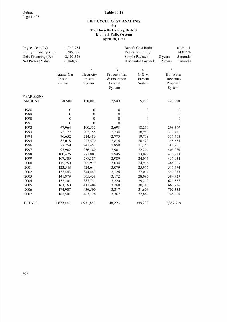
8/12/2019 Costing & Analysis for Engineering
http://slidepdf.com/reader/full/costing-analysis-for-engineering 34/48
Output Table 17.18
Page 1 of 5
LIFE CYCLE COST ANALYSIS
for
The Horsefly Heating District
Klamath Falls, Oregon
April 28, 1987
Project Cost (Pv) 1,759.954 Benefit Cost Ratio 0.39 to 1
Equity Financing (Pv) 295,078 Return on Equity 14.825%
Debt Financing (Pv) 2,100,526 Simple Payback 8 years 5 months Net Present Value -1,068,686 Discounted Payback 12 years 2 months
1 2 3 4 5
Natural Gas Electricity Property Tax O & M Hot Water
Present Present & Insurance Present Revenues
System System Present System Proposed
System System
YEAR ZERO
AMOUNT 50,500 150,000 2,500 15,000 220,000
1988 0 0 0 0 0
1989 0 0 0 0 0
1990 0 0 0 0 0
1991 0 0 0 0 0
1992 67,964 190,532 2,693 18,250 298,599
1993 72,177 202,155 2,734 18,980 317,411
1994 76,652 214,486 2,775 19,739 337,408
1995 82,018 227,570 2,816 20,529 358,665
1996 87,759 241,452 2,858 21,350 381,261
1997 93,902 256,180 2,901 22,204 405,280
1998 100,476 271,807 2,945 23,092 430,813
1999 107,509 288,387 2,989 24,015 457,954
2000 115,250 305,979 3,034 24,976 486,805
2001 123,548 324,644 3,079 25,975 517,474 2002 132,443 344,447 3,126 27,014 550,075
2003 141,979 365,458 3,172 28,095 584,729
2004 152,201 387,751 3,220 29,219 621,567
2005 163,160 411,404 3,268 30,387 660,726
2006 174,907 436,500 3,317 31,603 702,352
2007 187,501 463,126 3,367 32,867 746,600
TOTALS: 1,879,446 4,931,880 48,296 398,293 7,857,719
392
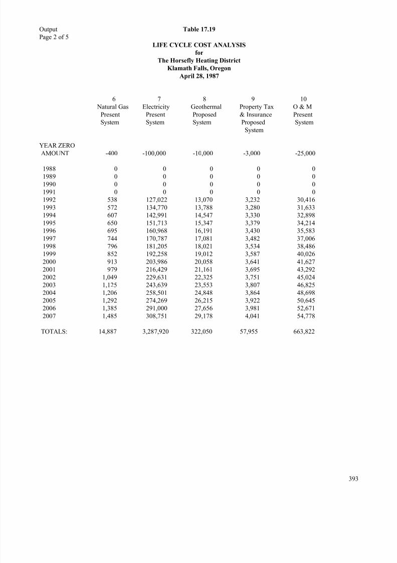
8/12/2019 Costing & Analysis for Engineering
http://slidepdf.com/reader/full/costing-analysis-for-engineering 35/48
Output Table 17.19
Page 2 of 5
LIFE CYCLE COST ANALYSIS
for
The Horsefly Heating District
Klamath Falls, Oregon
April 28, 1987
6 7 8 9 10 Natural Gas Electricity Geothermal Property Tax O & M
Present Present Proposed & Insurance Present
System System System Proposed System
System
YEAR ZERO
AMOUNT -400 -100,000 -10,000 -3,000 -25,000
1988 0 0 0 0 0
1989 0 0 0 0 0
1990 0 0 0 0 0
1991 0 0 0 0 0
1992 538 127,022 13,070 3,232 30,416
1993 572 134,770 13,788 3,280 31,633
1994 607 142,991 14,547 3,330 32,898
1995 650 151,713 15,347 3,379 34,214
1996 695 160,968 16,191 3,430 35,583
1997 744 170,787 17,081 3,482 37,006
1998 796 181,205 18,021 3,534 38,486
1999 852 192,258 19,012 3,587 40,026
2000 913 203,986 20,058 3,641 41,627
2001 979 216,429 21,161 3,695 43,292
2002 1,049 229,631 22,325 3,751 45,024
2003 1,125 243,639 23,553 3,807 46,825
2004 1,206 258,501 24,848 3,864 48,698 2005 1,292 274,269 26,215 3,922 50,645
2006 1,385 291,000 27,656 3,981 52,671
2007 1,485 308,751 29,178 4,041 54,778
TOTALS: 14,887 3,287,920 322,050 57,955 663,822
393
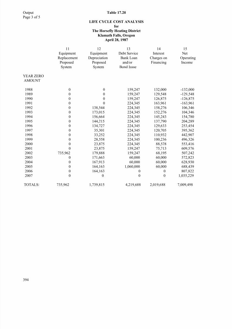
8/12/2019 Costing & Analysis for Engineering
http://slidepdf.com/reader/full/costing-analysis-for-engineering 36/48
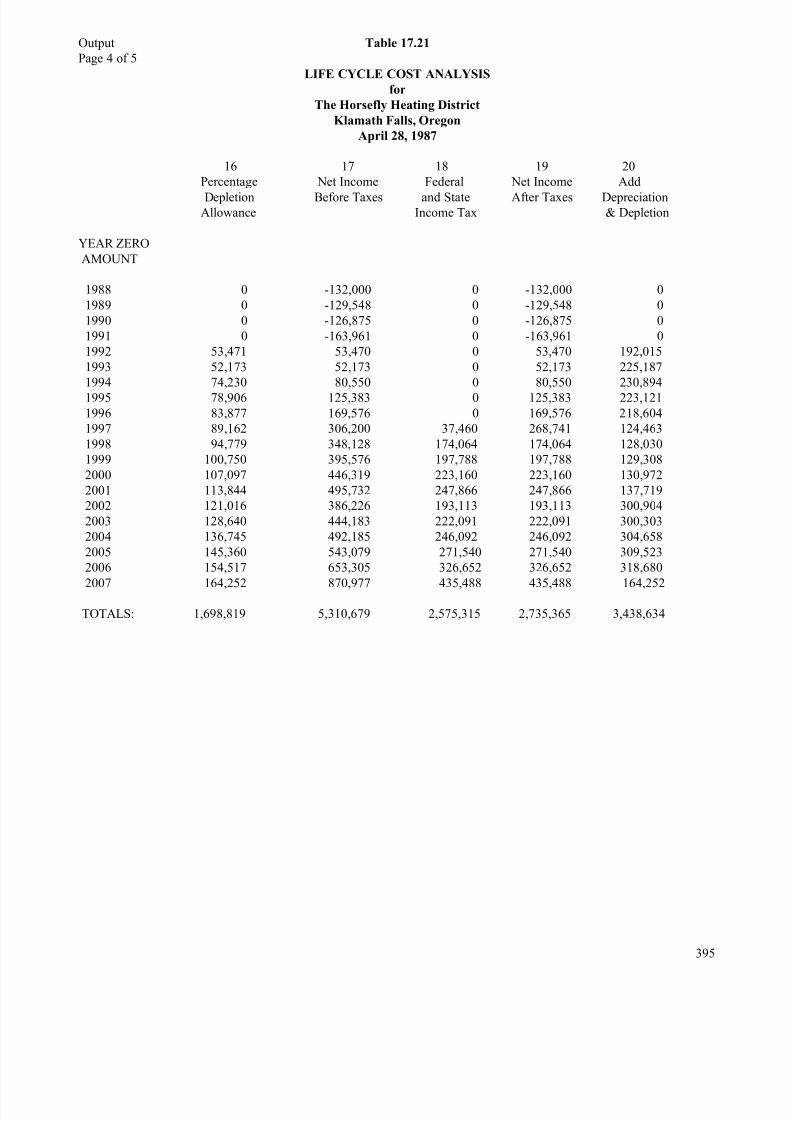
8/12/2019 Costing & Analysis for Engineering
http://slidepdf.com/reader/full/costing-analysis-for-engineering 37/48
Output Table 17.21
Page 4 of 5
LIFE CYCLE COST ANALYSIS
for
The Horsefly Heating District
Klamath Falls, Oregon
April 28, 1987
16 17 18 19 20
Percentage Net Income Federal Net Income Add
Depletion Before Taxes and State After Taxes Depreciation Allowance Income Tax & Depletion
YEAR ZERO
AMOUNT
1988 0 -132,000 0 -132,000 0
1989 0 -129,548 0 -129,548 0
1990 0 -126,875 0 -126,875 0
1991 0 -163,961 0 -163,961 0
1992 53,471 53,470 0 53,470 192,015
1993 52,173 52,173 0 52,173 225,187
1994 74,230 80,550 0 80,550 230,894
1995 78,906 125,383 0 125,383 223,121
1996 83,877 169,576 0 169,576 218,604
1997 89,162 306,200 37,460 268,741 124,463
1998 94,779 348,128 174,064 174,064 128,030
1999 100,750 395,576 197,788 197,788 129,308
2000 107,097 446,319 223,160 223,160 130,972
2001 113,844 495,732 247,866 247,866 137,719
2002 121,016 386,226 193,113 193,113 300,904
2003 128,640 444,183 222,091 222,091 300,303
2004 136,745 492,185 246,092 246,092 304,658
2005 145,360 543,079 271,540 271,540 309,523
2006 154,517 653,305 326,652 326,652 318,680
2007 164,252 870,977 435,488 435,488 164,252
TOTALS: 1,698,819 5,310,679 2,575,315 2,735,365 3,438,634
395
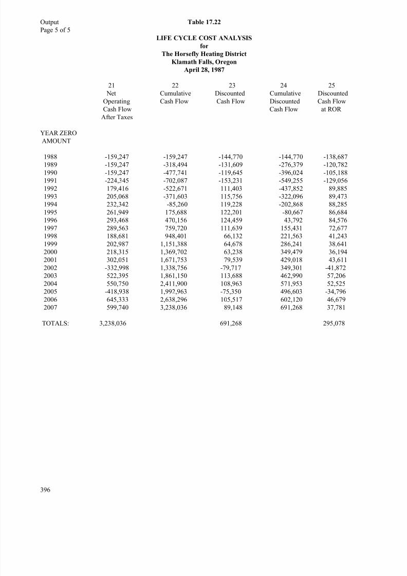
8/12/2019 Costing & Analysis for Engineering
http://slidepdf.com/reader/full/costing-analysis-for-engineering 38/48
Output Table 17.22
Page 5 of 5
LIFE CYCLE COST ANALYSIS
for
The Horsefly Heating District
Klamath Falls, Oregon
April 28, 1987
21 22 23 24 25
Net Cumulative Discounted Cumulative Discounted
Operating Cash Flow Cash Flow Discounted Cash FlowCash Flow Cash Flow at ROR
After Taxes
YEAR ZERO
AMOUNT
1988 -159,247 -159,247 -144,770 -144,770 -138,687
1989 -159,247 -318,494 -131,609 -276,379 -120,782
1990 -159,247 -477,741 -119,645 -396,024 -105,188
1991 -224,345 -702,087 -153,231 -549,255 -129,056
1992 179,416 -522,671 111,403 -437,852 89,885
1993 205,068 -371,603 115,756 -322,096 89,473
1994 232,342 -85,260 119,228 -202,868 88,285
1995 261,949 175,688 122,201 -80,667 86,684
1996 293,468 470,156 124,459 43,792 84,576
1997 289,563 759,720 111,639 155,431 72,677
1998 188,681 948,401 66,132 221,563 41,243
1999 202,987 1,151,388 64,678 286,241 38,641
2000 218,315 1,369,702 63,238 349,479 36,194
2001 302,051 1,671,753 79,539 429,018 43,611
2002 -332,998 1,338,756 -79,717 349,301 -41,872
2003 522,395 1,861,150 113,688 462,990 57,206
2004 550,750 2,411,900 108,963 571,953 52,525
2005 -418,938 1,992,963 -75,350 496,603 -34,796
2006 645,333 2,638,296 105,517 602,120 46,679 2007 599,740 3,238,036 89,148 691,268 37,781
TOTALS: 3,238,036 691,268 295,078
396
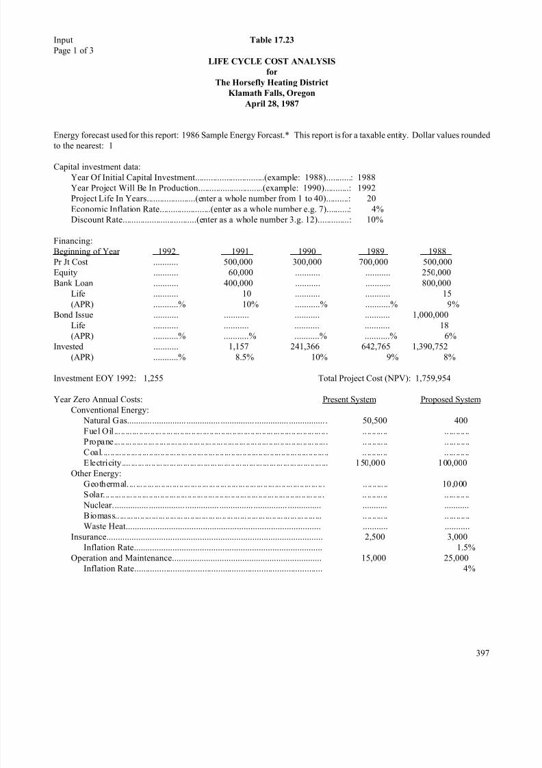
8/12/2019 Costing & Analysis for Engineering
http://slidepdf.com/reader/full/costing-analysis-for-engineering 39/48
Input Table 17.23
Page 1 of 3
LIFE CYCLE COST ANALYSIS
for
The Horsefly Heating District
Klamath Falls, Oregon
April 28, 1987
Energy forecast used for this report: 1986 Sample Energy Forcast.* This report is for a taxable entity. Dollar values roundedto the nearest: 1
Capital investment data:
Year Of Initial Capital Investment...............................(example: 1988)...........: 1988
Year Project Will Be In Production.............................(example: 1990)...........: 1992
Project Life In Years......................(enter a whole number from 1 to 40)..........: 20
Economic Inflation Rate.......................(enter as a whole number e.g. 7)..........: 4%
Discount Rate.................................(enter as a whole number 3.g. 12)..............: 10%
Financing:
Beginning of Year 1992 1991 1990 1989 1988
Pr Jt Cost ........... 500,000 300,000 700,000 500,000
Equity ........... 60,000 ........... ........... 250,000
Bank Loan ........... 400,000 ........... ........... 800,000
Life ........... 10 ........... ........... 15
(APR) ...........% 10% ...........% ...........% 9%
Bond Issue ........... ........... ........... ........... 1,000,000
Life ........... ........... ........... ........... 18
(APR) ...........% ...........% ...........% ...........% 6%
Invested ........... 1,157 241,366 642,765 1,390,752
(APR) ...........% 8.5% 10% 9% 8%
Investment EOY 1992: 1,255 Total Project Cost (NPV): 1,759,954
Year Zero Annual Costs: Present System Proposed SystemConventional Energy:
Natural Gas........... ............... ............... ............... ............... ................ . 50,500 400
Fuel Oil... .. ... ... .. ... .. ... .. ... ... .. ... .. ... ... .. ... .. ... .. ... ... .. ... .. ... ... .. ... .. ... .. ... ... .. . .. .. .. ... .. .. ... .. .. ..
Propane... .. ... .. ... .. ... .. ... .. ... .. ... .. ... .. ... .. ... .. ... .. ... .. ... .. ... .. ... .. ... .. ... .. ... .. ... . .. .. .. ... .. .. ... .. .. ..
Coal. ... .. ... .. .. ... .. ... .. ... .. .. ... .. ... .. .. ... .. ... .. .. ... .. ... .. .. ... .. ... .. ... .. .. ... .. ... .. .. ... .. .. .. .. ... .. .. ... .. .. ..
Electricity.... ... ... ... .. ... ... ... ... ... ... ... ... ... ... ... .. ... ... ... ... ... ... ... ... ... ... ... .. ... ... 150,000 100,000
Other Energy:
Geothermal.... ... .. ... ... .. ... ... .. ... ... .. ... ... .. ... .. ... ... .. ... ... .. ... ... .. ... ... .. ... ... .. . .. .. .. ... .. 10,000
Solar. .. .. ... .. ... .. .. ... .. ... .. .. ... .. ... .. .. ... .. ... .. .. ... .. .. ... .. ... .. .. ... .. ... .. .. ... .. ... .. .. . .. .. .. ... .. .. ... .. .. ..
Nuclear. ............... ................ ............... ............... ............... ............... ........... ...........
Biomass.. ... ... ... .. ... ... ... .. ... ... ... .. ... ... ... ... .. ... ... ... .. ... ... ... .. ... ... ... ... .. ... ... .. .. .. ... .. .. ... .. .. ..
Waste Heat...................................................................................... ........... ...........
Insurance............................................................................................... 2,500 3,000Inflation Rate................................................................................... 1.5%
Operation and Maintenance.................................................................. 15,000 25,000
Inflation Rate................................................................................... 4%
397
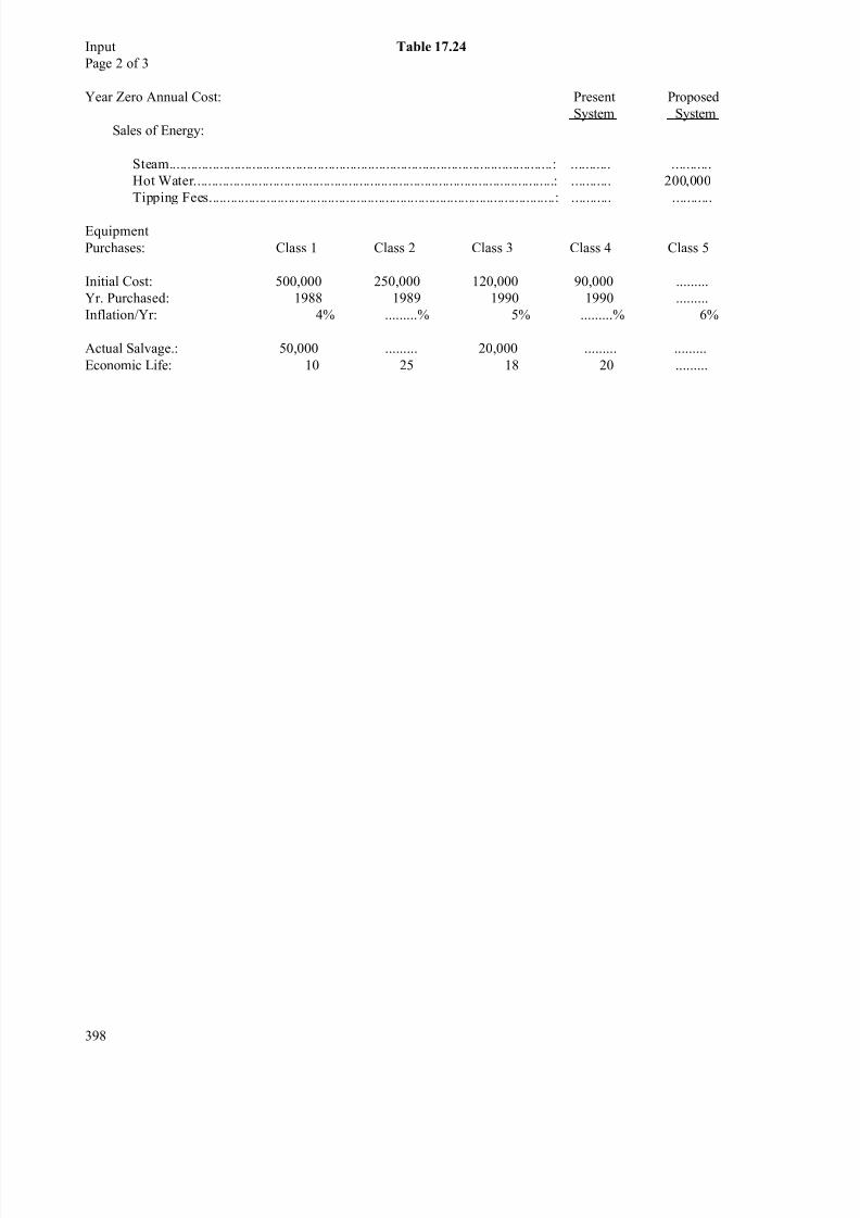
8/12/2019 Costing & Analysis for Engineering
http://slidepdf.com/reader/full/costing-analysis-for-engineering 40/48
Input Table 17.24
Page 2 of 3
Year Zero Annual Cost: Present Proposed
System System
Sales of Energy:
Steam..........................................................................................................: ........... ...........
Hot Water....................................................................................................: ........... 200,000
Tipping Fees................................................................................................: ........... ...........
Equipment
Purchases: Class 1 Class 2 Class 3 Class 4 Class 5
Initial Cost: 500,000 250,000 120,000 90,000 .........
Yr. Purchased: 1988 1989 1990 1990 .........
Inflation/Yr: 4% .........% 5% .........% 6%
Actual Salvage.: 50,000 ......... 20,000 ......... .........
Economic Life: 10 25 18 20 .........
398
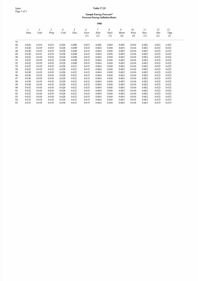
8/12/2019 Costing & Analysis for Engineering
http://slidepdf.com/reader/full/costing-analysis-for-engineering 41/48
Input Table 17.25
Page 3 of 3
Sample Energy Forecast*
Forecast Energy Inflation Rates
1986
1 2 3 4 5 6 7 8 9 10 11 12 13
Natu Fuel Prop Coal Elec Geot Sola Nucl Biom Wast Stea Hot Tipp
(1) (2) (3) (4) (5) (1) (2) (3)
_______________________________________________________________________________________________________________________________________
Yr
86 0.020 0.019 0.019 0.020 0.009 0.015 0.004 0.001 0.005 0.010 0.002 0.023 0.023
87 0.020 0.019 0.019 0.020 0.009 0.015 0.004 0.001 0.005 0.010 0.002 0.023 0.02388 0.020 0.019 0.019 0.020 0.009 0.015 0.004 0.001 0.005 0.010 0.002 0.023 0.023
89 0.020 0.019 0.019 0.020 0.009 0.015 0.004 0.001 0.005 0.010 0.002 0.023 0.023
90 0.022 0.019 0.019 0.020 0.009 0.015 0.004 0.001 0.005 0.010 0.002 0.023 0.023
91 0.022 0.019 0.019 0.020 0.009 0.015 0.004 0.001 0.005 0.010 0.002 0.023 0.023
92 0.022 0.019 0.019 0.020 0.009 0.015 0.004 0.001 0.005 0.010 0.002 0.023 0.023
93 0.022 0.019 0.019 0.020 0.021 0.015 0.004 0.001 0.005 0.010 0.002 0.023 0.023
94 0.022 0.019 0.019 0.020 0.021 0.015 0.004 0.001 0.005 0.010 0.002 0.023 0.023
95 0.030 0.019 0.019 0.020 0.021 0.015 0.004 0.001 0.005 0.010 0.002 0.023 0.023
96 0.030 0.019 0.019 0.020 0.021 0.015 0.004 0.001 0.005 0.010 0.002 0.023 0.023
97 0.030 0.019 0.019 0.020 0.021 0.015 0.004 0.001 0.005 0.010 0.002 0.023 0.023
98 0.030 0.019 0.019 0.020 0.021 0.015 0.004 0.001 0.005 0.010 0.002 0.023 0.023
99 0.030 0.019 0.019 0.020 0.021 0.015 0.004 0.001 0.005 0.010 0.002 0.023 0.023
00 0.032 0.018 0.018 0.020 0.021 0.015 0.004 0.001 0.005 0.010 0.002 0.023 0.023
01 0.032 0.018 0.018 0.020 0.021 0.015 0.004 0.001 0.005 0.010 0.002 0.023 0.023
02 0.032 0.018 0.018 0.020 0.021 0.015 0.004 0.001 0.005 0.010 0.002 0.023 0.023
03 0.032 0.018 0.018 0.020 0.021 0.015 0.004 0.001 0.005 0.010 0.002 0.023 0.023
04 0.032 0.018 0.018 0.020 0.021 0.015 0.004 0.001 0.005 0.010 0.002 0.023 0.023
05 0.032 0.018 0.018 0.020 0.021 0.015 0.004 0.001 0.005 0.010 0.002 0.023 0.023
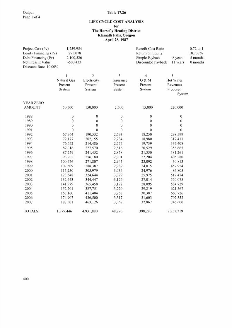
8/12/2019 Costing & Analysis for Engineering
http://slidepdf.com/reader/full/costing-analysis-for-engineering 42/48
Output Table 17.26
Page 1 of 4
LIFE CYCLE COST ANALYSIS
for
The Horsefly Heating District
Klamath Falls, Oregon
April 28, 1987
Project Cost (Pv) 1,759.954 Benefit Cost Ratio 0.72 to 1
Equity Financing (Pv) 295,078 Return on Equity 18.737%
Debt Financing (Pv) 2,100,526 Simple Payback 8 years 5 months Net Present Value -500,433 Discounted Payback 11 years 0 months
Discount Rate 10.00%
1 2 3 4 5
Natural Gas Electricity Insurance O & M Hot Water
Present Present Present Present Revenues
System System System System Proposed
System
YEAR ZERO
AMOUNT 50,500 150,000 2,500 15,000 220,000
1988 0 0 0 0 0
1989 0 0 0 0 0
1990 0 0 0 0 0
1991 0 0 0 0 0
1992 67,964 190,532 2,693 18,250 298,599
1993 72,177 202,155 2,734 18,980 317,411
1994 76,652 214,486 2,775 19,739 337,408
1995 82,018 227,570 2,816 20,529 358,665
1996 87,759 241,452 2,858 21,350 381,261
1997 93,902 256,180 2,901 22,204 405,280
1998 100,476 271,807 2,945 23,092 430,813
1999 107,509 288,387 2,989 24,015 457,954
2000 115,250 305,979 3,034 24,976 486,805 2001 123,548 324,644 3,079 25,975 517,474
2002 132,443 344,447 3,126 27,014 550,075
2003 141,979 365,458 3,172 28,095 584,729
2004 152,201 387,751 3,220 29,219 621,567
2005 163,160 411,404 3,268 30,387 660,726
2006 174,907 436,500 3,317 31,603 702,352
2007 187,501 463,126 3,367 32,867 746,600
TOTALS: 1,879,446 4,931,880 48,296 398,293 7,857,719
400
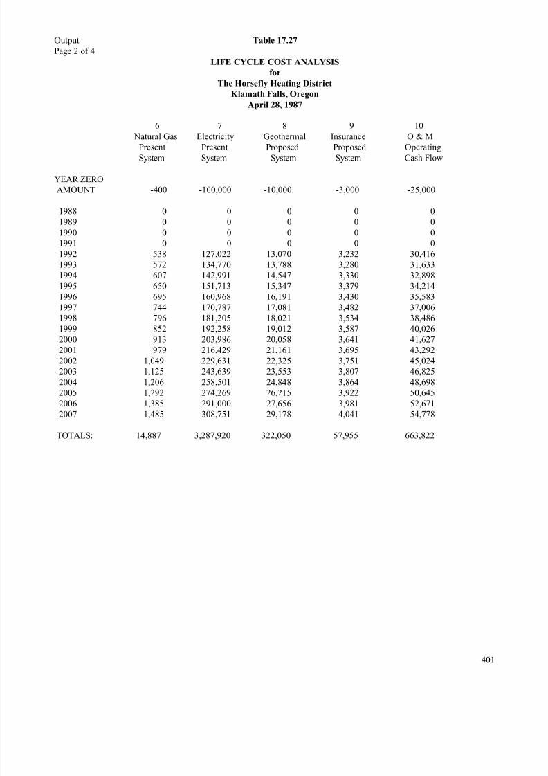
8/12/2019 Costing & Analysis for Engineering
http://slidepdf.com/reader/full/costing-analysis-for-engineering 43/48
Output Table 17.27
Page 2 of 4
LIFE CYCLE COST ANALYSIS
for
The Horsefly Heating District
Klamath Falls, Oregon
April 28, 1987
6 7 8 9 10
Natural Gas Electricity Geothermal Insurance O & M Present Present Proposed Proposed Operating
System System System System Cash Flow
YEAR ZERO
AMOUNT -400 -100,000 -10,000 -3,000 -25,000
1988 0 0 0 0 0
1989 0 0 0 0 0
1990 0 0 0 0 0
1991 0 0 0 0 0
1992 538 127,022 13,070 3,232 30,416
1993 572 134,770 13,788 3,280 31,633
1994 607 142,991 14,547 3,330 32,898
1995 650 151,713 15,347 3,379 34,214
1996 695 160,968 16,191 3,430 35,583
1997 744 170,787 17,081 3,482 37,006
1998 796 181,205 18,021 3,534 38,486
1999 852 192,258 19,012 3,587 40,026
2000 913 203,986 20,058 3,641 41,627
2001 979 216,429 21,161 3,695 43,292
2002 1,049 229,631 22,325 3,751 45,024
2003 1,125 243,639 23,553 3,807 46,825
2004 1,206 258,501 24,848 3,864 48,698
2005 1,292 274,269 26,215 3,922 50,645
2006 1,385 291,000 27,656 3,981 52,671 2007 1,485 308,751 29,178 4,041 54,778
TOTALS: 14,887 3,287,920 322,050 57,955 663,822
401
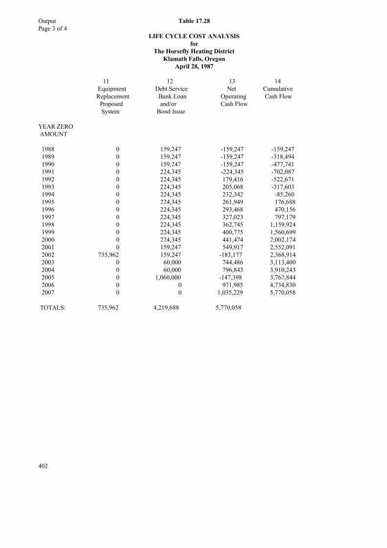
8/12/2019 Costing & Analysis for Engineering
http://slidepdf.com/reader/full/costing-analysis-for-engineering 44/48
Output Table 17.28
Page 3 of 4
LIFE CYCLE COST ANALYSIS
for
The Horsefly Heating District
Klamath Falls, Oregon
April 28, 1987
11 12 13 14
Equipment Debt Service Net Cumulative
Replacement Bank Loan Operating Cash Flow Proposed and/or Cash Flow
System Bond Issue
YEAR ZERO
AMOUNT
1988 0 159,247 -159,247 -159,247
1989 0 159,247 -159,247 -318,494
1990 0 159,247 -159,247 -477,741
1991 0 224,345 -224,345 -702,087
1992 0 224,345 179,416 -522,671
1993 0 224,345 205,068 -317,603
1994 0 224,345 232,342 -85,260
1995 0 224,345 261,949 176,688
1996 0 224,345 293,468 470,156
1997 0 224,345 327,023 797,179
1998 0 224,345 362,745 1,159,924
1999 0 224,345 400,775 1,560,699
2000 0 224,345 441,474 2,002,174
2001 0 159,247 549,917 2,552,091
2002 735,962 159,247 -183,177 2,368,914
2003 0 60,000 744,486 3,113,400
2004 0 60,000 796,843 3,910,243
2005 0 1,060,000 -147,398 3,762,844
2006 0 0 971,985 4,734,830 2007 0 0 1,035,229 5,770,058
TOTALS: 735,962 4,219,688 5,770,058
402
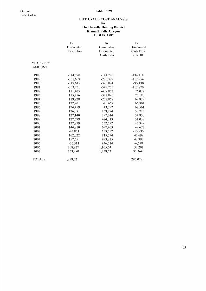
8/12/2019 Costing & Analysis for Engineering
http://slidepdf.com/reader/full/costing-analysis-for-engineering 45/48
Output Table 17.29
Page 4 of 4
LIFE CYCLE COST ANALYSIS
for
The Horsefly Heating District
Klamath Falls, Oregon
April 28, 1987
15 16 17
Discounted Cumulative Discounted
Cash Flow Discounted Cash Flow Cash Flow at ROR
YEAR ZERO
AMOUNT
1988 -144,770 -144,770 -134,118
1989 -131,609 -276,379 -112,954
1990 -119,645 -396,024 -95,130
1991 -153,231 -549,255 -112,870
1992 111,403 -437,852 76,022
1993 115,756 -322,096 73,180
1994 119,228 -202,868 69,829
1995 122,201 -80,667 66,304
1996 124,459 43,792 62,561
1997 126,081 169,874 58,713
1998 127,140 297,014 54,850
1999 127,699 424,713 51,037
2000 127,879 552,592 47,349
2001 144,810 697,403 49,673
2002 -43,851 653,552 -13,935
2003 162,022 815,574 47,699
2004 157,651 973,225 42,997
2005 -26,511 946,714 -6,698
2006 158,927 1,105,641 37,201
2007 153,880 1,259,521 33,369
TOTALS: 1,259,521 295,078
403
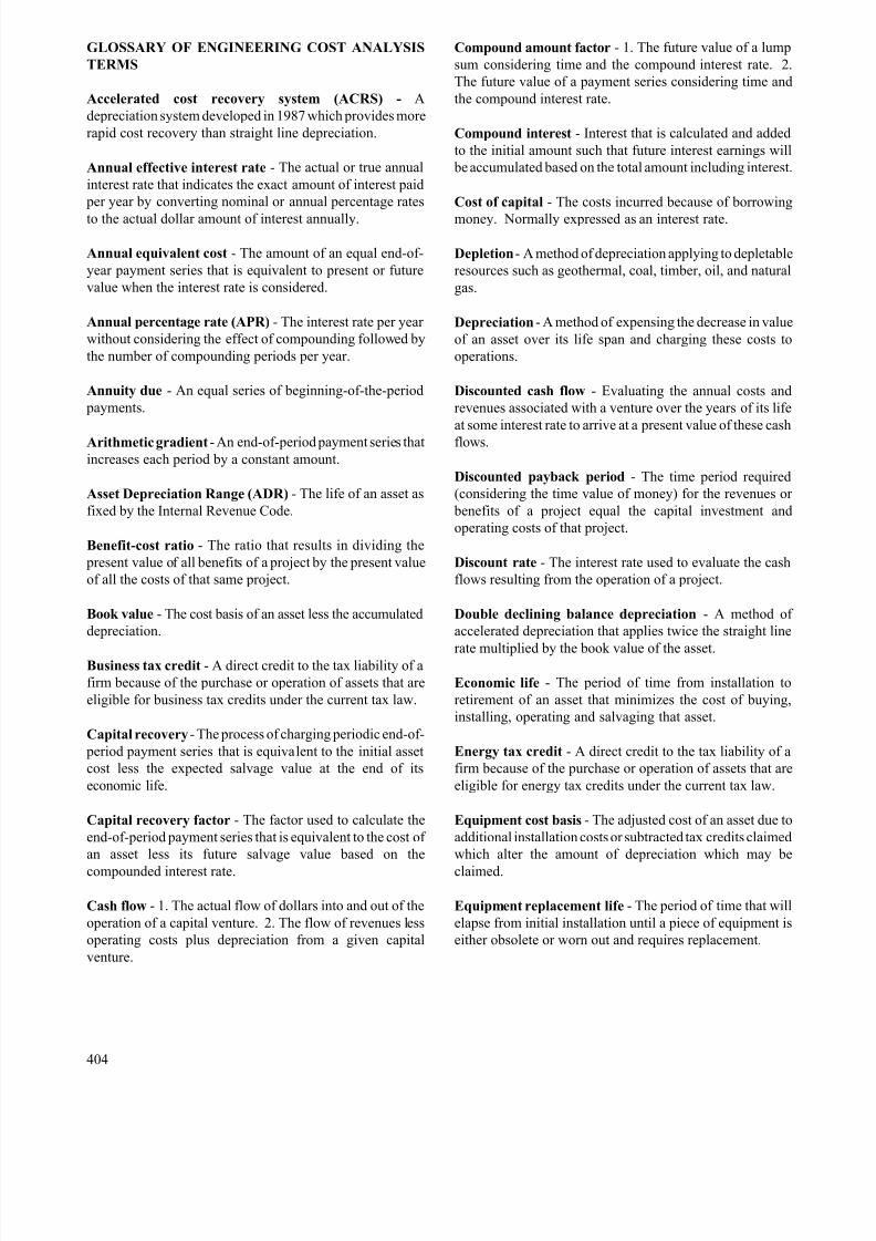
8/12/2019 Costing & Analysis for Engineering
http://slidepdf.com/reader/full/costing-analysis-for-engineering 46/48
GLOSSARY OF ENGINEERING COST ANALYSIS
TERMS
Accelerated cost recovery system (ACRS) - A
depreciation system developed in 1987 which provides more
rapid cost recovery than straight line depreciation.
Annual effective interest rate - The actual or true annual
interest rate that indicates the exact amount of interest paid
per year by converting nominal or annual percentage rates
to the actual dollar amount of interest annually.
Annual equivalent cost - The amount of an equal end-of-
year payment series that is equivalent to present or future
value when the interest rate is considered.
Annual percentage rate (APR) - The interest rate per year
without considering the effect of compounding followed by
the number of compounding periods per year.
Annuity due - An equal series of beginning-of-the-period
payments.
Arithmetic gradient - An end-of-period payment series that
increases each period by a constant amount.
Asset Depreciation Range (ADR) - The life of an asset as
fixed by the Internal Revenue Code.
Benefit-cost ratio - The ratio that results in dividing the
present value of all benefits of a project by the present value
of all the costs of that same project.
Book value - The cost basis of an asset less the accumulated
depreciation.
Business tax credit - A direct credit to the tax liability of a
firm because of the purchase or operation of assets that are
eligible for business tax credits under the current tax law.
Capital recovery - The process of charging periodic end-of-
period payment series that is equivalent to the initial asset
cost less the expected salvage value at the end of its
economic life.
Capital recovery factor - The factor used to calculate the
end-of-period payment series that is equivalent to the cost of
an asset less its future salvage value based on the
compounded interest rate.
Cash flow - 1. The actual flow of dollars into and out of the
operation of a capital venture. 2. The flow of revenues less
operating costs plus depreciation from a given capital
venture.
404
Compound amount factor - 1. The future value of a lump
sum considering time and the compound interest rate. 2.
The future value of a payment series considering time and
the compound interest rate.
Compound interest - Interest that is calculated and added
to the initial amount such that future interest earnings will
be accumulated based on the total amount including interest.
Cost of capital - The costs incurred because of borrowing
money. Normally expressed as an interest rate.
Depletion - A method of depreciation applying to depletable
resources such as geothermal, coal, timber, oil, and natural
gas.
Depreciation - A method of expensing the decrease in value
of an asset over its life span and charging these costs to
operations.
Discounted cash flow - Evaluating the annual costs and
revenues associated with a venture over the years of its life
at some interest rate to arrive at a present value of these cash
flows.
Discounted payback period - The time period required
(considering the time value of money) for the revenues or
benefits of a project equal the capital investment and
operating costs of that project.
Discount rate - The interest rate used to evaluate the cash
flows resulting from the operation of a project.
Double declining balance depreciation - A method of
accelerated depreciation that applies twice the straight line
rate multiplied by the book value of the asset.
Economic life - The period of time from installation to
retirement of an asset that minimizes the cost of buying,
installing, operating and salvaging that asset.
Energy tax credit - A direct credit to the tax liability of a
firm because of the purchase or operation of assets that are
eligible for energy tax credits under the current tax law.
Equipment cost basis - The adjusted cost of an asset due to
additional installation costs or subtracted tax credits claimed
which alter the amount of depreciation which may be
claimed.
Equipment replacement life - The period of time that will
elapse from initial installation until a piece of equipment is
either obsolete or worn out and requires replacement.
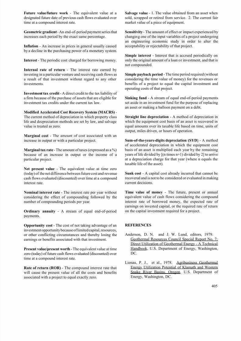
8/12/2019 Costing & Analysis for Engineering
http://slidepdf.com/reader/full/costing-analysis-for-engineering 47/48
Future value/future work - The equivalent value at a
designated future date of previous cash flows evaluated over
time at a compound interest rate.
Geometric gradient - An end-of-period payment series that
increases each period by the exact same percentage.
Inflation - An increase in prices in general usually caused
by a decline in the purchasing power of a monetary system.
Interest - The periodic cost charged for borrowing money.
Internal rate of return - The interest rate earned by
investing in a particular venture and receiving cash flows as
a result of that investment without regard to any other
investments.
Investment tax credit - A direct credit to the tax liability of
a firm because of the purchase of assets that are eligible for
investment tax credits under the current tax law.
Modified Accelerated Cost Recovery System (MACRS) -
The current method of depreciation in which property class
life and decpreciation methods are set by law, and salvage
value is treated as zero.
Marginal cost - The amount of cost associated with an
increase in output or with a particular project.
Marginal tax rate - The amount of taxes (expressed as a %)
because of an increase in output or the income of a
particular project.
Net present value - The equivalent value at time zero
(today) of the net difference between future cost and revenue
cash flows evaluated (discounted) over time at a compoundinterest rate.
Nominal interest rate - The interest rate per year without
considering the effect of compounding followed by the
number of compounding periods per year.
Ordinary annuity - A stream of equal end-of-period
payments.
Opportunity cost - The cost of not taking advantage of an
investment opportunity because of limited capital, resources,
or other conflicting circumstances and thereby losing the
earnings or benefits associated with that investment.
Present value/present worth - The equivalent value at time
zero (today) of future cash flows evaluated (discounted) over
time at a compound interest rate.
Rate of return (ROR) - The compound interest rate that
will cause the present value of all the costs and benefits
associated with a project to equal exactly zero.
Salvage value - 1. The value obtained from an asset when
sold, scrapped or retired from service. 2. The current fair
market value of a piece of equipment.
Sensitivity - The amount of effect or impact experienced by
changing one of the input variables of a project undergoing
an engineering economic study in order to alter the
acceptability or rejectability of that project.
Simple interest - Interest that is accrued periodically on
only the original amount of a loan or investment, and that isnot compounded.
Simple payback period - The time period required (without
considering the time value of money) for the revenues or
benefits of a project to equal the capital investment and
operating costs of that project.
Sinking fund - A stream of equal end-of-period payments
set aside in an investment fund for the purpose of replacing
an asset or making a balloon payment on a debt.
Straight line depreciation - A method of depreciation in
which the equipment cost basis of an asset is recovered in
equal amounts over its taxable life based on time, units of
output, miles driven, or hours of operation.
Sum-of-the-years-digits depreciation (SYD) - A method
of accelerated depreciation in which the equipment cost
basis of an asset is multiplied each year by the remaining
years of life divided by [(n times n+1) divided by 2] to arrive
at a depreciation charge for that year (where n equals the
taxable life of the asset).
Sunk cost - A capital cost already incurred that cannot be
recovered and is not to be considered or evaluated in makingcurrent decisions.
Time value of money - The future, present or annual
equivalent value of cash flows considering the compound
interest rate of borrowed money, the expected rate of
earnings on invested capital, or the required rate of return
on the capital investment required for a project.
REFERENCES
Anderson, D. N. and J. W. Lund, editors, 1979.
Geothermal Resources Council Special Report No. 7:Direct Utilization of Geothermal Energy - A Technical
Handbook, U.S. Department of Energy, Washington,
DC.
Lienau, P. J., et al., 1978. Agribusiness Geothermal
Energy Utilization Potential of Klamath and Western
Snake River Basins, Oregon, U.S. Department of
Energy, Washington, DC.
405
8/12/2019 Costing & Analysis for Engineering
http://slidepdf.com/reader/full/costing-analysis-for-engineering 48/48
Newnan, D. G., 1988. Engineering Economic Analysis,
3rd edition, Engineering Press Inc., San Jose, CA.
Riggs, J. L. and T. M. West, 1986. Engineering
Economics, 3rd edition, McGraw-Hill Book Co.,
NY.
Thuesen, G. H. and W. J. Fabrycky, 1984. Engineering
Economy, 6th edition, Prentice-Hall Inc., Englewood
Cliffs, NJ.