Cost Optimum Design of Posttensioned I-Girder Bridge … · Cost Optimum Design of Posttensioned I-Girder Bridge Using Global Optimization Algorithm Raquib Ahsan1; Shohel Rana2; and

Cost Optimum Design of Posttensioned I-Girder BridgeUsing Global Optimization Algorithm

Raquib Ahsan1; Shohel Rana2; and Sayeed Nurul Ghani3

Abstract: This paper presents an optimization approach to the design of simply supported, post-tensioned, prestressed concrete I-girderbridges. The objective is to minimize the total cost of the structure, considering cost of materials, fabrication, and installation. For a particulargirder span and bridge width, the design variables considered for cost minimization of the bridge system are girder spacing, various cross-sectional dimensions of the girder, number of strands per tendon, number of tendons, tendon layout and configuration, slab thickness, slabrebar, and shear rebar for the girder. Explicit constraints on the design variables are developed on the basis of geometric requirements,practical conditions for construction, and code restrictions. Implicit constraints for design are formulated as per the American Associationof State Highway and Transportation Officials (AASHTO) Standard Specifications. The optimization problem is characterized by having acombination of continuous, discrete, and integer sets of design variables and multiple local minima. An optimization algorithm, evolutionaryoperation (EVOP), is used that is capable of locating directly with high probability the global minimum without requiring information ongradient or subgradient of the objective function. The present optimization approach is used for a real-life bridge project, leading to a feasibleand acceptable design resulting in around 35% savings in cost per square meter of the deck area. Computational time required for opti-mization of the present problem is only a few seconds. Because constant design parameters have influence on the optimum design, this costminimization procedure is performed for a range of such parameters. DOI: 10.1061/(ASCE)ST.1943-541X.0000458. © 2012 AmericanSociety of Civil Engineers.

CE Database subject headings: Cost; Structural design; Girder bridges; Post tensioning; Optimization; Algorithms.

Author keywords: Cost optimum design; Prestressed concrete; Post-tensioned girder bridge; Constrained global optimization.

Introduction

Prestressed concrete (PC) I-girder bridge systems are ideal as shortto medium span (20 to 60 m) highway bridges because of theirmoderate self weight, structural efficiency, ease of fabrication, fastconstruction, low initial cost, long life expectancy, low mainte-nance, simple deck removal, and replacement (Precast/PrestressedConcrete Institute (PCI) 2003). To compete with steel bridge sys-tems, the design of PC I-girder bridges should lead to the most eco-nomical use of materials (PCI 1999). Large numbers of designvariables are involved in the design process of the PC I-girderbridges, and all variables are related to one other, leading to numer-ous alternative feasible designs. In the traditional design approach,bridge engineers follow iterative procedures for designing pre-stressed I-girder bridge structures. There is no formal attempt toreach the best design in the strict mathematical sense of minimizingcost, weight, or volume. The design process relies solely on thedesigners’ experience, intuition, and ingenuity resulting in a highcost in material, time, and human effort.

The optimum design procedure is an alternative to the tradi-tional design approach. Such a design usually implies the mosteconomic structure without impairing any of its functional pur-poses. The optimization technique transforms the conventional de-sign process of trial and error to a formal, systematic, and digitalcomputer-based automated procedure that yields a design that is thebest in the designer-specified figure of merit—the goodness factorof design. Advances in numerical optimization methods, computer-based numerical tools for analysis, and design of structures andavailability of powerful computing hardware have all significantlyaided the design process. So, the time is now appropriate to performresearch on realistically optimizing three-dimensional structures,especially large structures with hundreds of members where opti-mization can result in substantial savings (Adeli and Sarma 2006).Large and important projects containing I-girder bridge structureshave the potential for substantial cost reduction through applicationof optimum design methodology and thus, will be of great value topracticing engineers.

Many research performed on structural optimization deal withminimization of the weight of the structure (Vanderplaats 1984;Arora 1989; Adeli and Kamal 1993; Adeli 1994; Cohn andDinovitzer 1994; Adeli and Sarma 2006). For concrete structures,however, the approach to optimum design may take the form of costminimization problem because different materials are involved. Areview of articles pertaining to the cost optimization of concretestructures is presented by Sarma and Adeli (1998) and the samefor concrete bridge structures by Hassanain and Loov (2003).Torres et al. (1966) and Fereig (1985, 1996) presented the mini-mum cost design of prestressed concrete bridges using the linearprogramming method. Cohn and MacRae (1984a, b) studied theminimum cost design of fully prestressed and partially prestressedconcrete I-beams with fixed cross-sectional geometry using a

1Professor, Dept. of Civil Engineering, Bangladesh Univ. of Engineer-ing and Technology (BUET), Dhaka-1000, Bangladesh (correspondingauthor). E-mail: [email protected]

2Assistant Professor, Dept. of Civil Engineering, Bangladesh Univ. ofEngineering and Technology (BUET), Dhaka-1000, Bangladesh. E-mail:[email protected]

3Principal Engineer/Consultant, Optimum System Designers, 2387 ESkipping Rock Way, Tucson, AZ85737. E-mail: [email protected]

Note. This manuscript was submitted on June 10, 2010; approved onJune 15, 2011; published online on June 17, 2011. Discussion period openuntil July 1, 2012; separate discussions must be submitted for individual pa-pers. This paper is part of the Journal of Structural Engineering, Vol. 138,No.2,February1,2012.©ASCE,ISSN0733-9445/2012/2-273–284/$25.00.

JOURNAL OF STRUCTURAL ENGINEERING © ASCE / FEBRUARY 2012 / 273

Downloaded 08 Jun 2012 to 150.135.239.97. Redistribution subject to ASCE license or copyright. Visit http://www.ascelibrary.org

http://dx.doi.org/10.1061/(ASCE)ST.1943-541X.0000458




nonlinear programming technique. Jones (1985), Yu et al. (1986),and Fereig (1994) formulated a minimum cost design of the PC boxgirder bridge system. Lounis and Cohn (1993) presented a costoptimization method for short and medium span pretensionedPC I-girder bridge. Nonlinear programming methods (projectedLagrangian method and sieve-search technique) were utilized toobtain the minimum superstructure cost as a criterion for the bestdesign. They first found the maximum feasible girder spacingfor each standard Canadian Precast Concrete I (CPCI) girderand American Association of State Highway and TransportationOfficials (AASHTO) sections and then minimized the prestressedand non-prestressed reinforcement in the I-girder and the deck.Costs of individual components, such as the girders or the deck,were then minimized. No attempt was made regarding ascertainingthe optimal girder cross section and the spacing that may minimizethe total cost inclusive of the cost of the bridge deck. Sirca andAdeli (2005) presented an optimization method for minimizingthe total cost of the pretensioned PC I-beam bridge system by con-sidering the concrete area, deck slab thickness, reinforcement, sur-face area of formwork, and number of beams as design variables.The problem is formulated as a mixed integer-discrete nonlinearprogramming problem and solved by using a patented robust neuraldynamics model. They did not consider cross-sectional dimensionsas design variables; instead, they used standard AASHTO sections.In the studies discussed previously, the prestressing strands/tendonswere assumed to be located at a fixed eccentricity. In reality, how-ever, strands/tendons are located at different positions at a crosssection of the girder. The longitudinal profiles of tendons also varydepending on their location on a cross section. Again, a lump-sumvalue (a certain percentage of initial prestress) of prestress losseswas estimated in these studies. As prestress losses are implicit func-tions of material properties, girder geometry and constructionmethod, a more accurate assessment of these losses, however, isrequired for greater precision. Ayvaz and Aydin (2009) presenteda study on minimizing the cost of a pretensioned PC I-girder bridgethrough topological and shape optimization. This topological andshape optimization of the bridge system were performed togetherwith a genetic algorithm (GA).

In this paper, an optimum design approach for simply supportedpost-tensioned I-girder bridges with cross-sectional dimensions andtendon arrangements as design variables is developed, while con-sidering the cost of materials, including fabrication and installation.The bridge system consists of precast girders with a cast-in situreinforced concrete deck. A large number of design variables andconstraints are considered, and an optimization algorithm evolu-tionary operation (EVOP) (Ghani 1989) is used. The algorithmis capable of dealing with an objective function containing a mixof integer, discrete, and continuous design variables and locatingdirectly the global minimum with a high probability. The EVOPcode is written in FORTRAN. The main program that executesEVOP is developed in C++ language to formulate the mathematicalexpressions required for analysis and design of the bridge system,to define a starting point inside the feasible space, and to inputEVOP control parameters. Three functions are also defined in thisprogram: an objective function, an explicit constraint function, andan implicit constraint function, all required by the EVOP code. Allare then compiled, linked, and executed to perform a cost optimumdesign of the previously discussed bridge system. A case study ispresented by comparing the optimum design obtained by thepresent approach with the design of a recently constructed struc-ture. A parametric study is also conducted by optimizing the designof post-tensioned PC I-girder bridges for different sets of values ofconstant parameters.

Problem Formulation

Design Variables and Constant Design Parameters

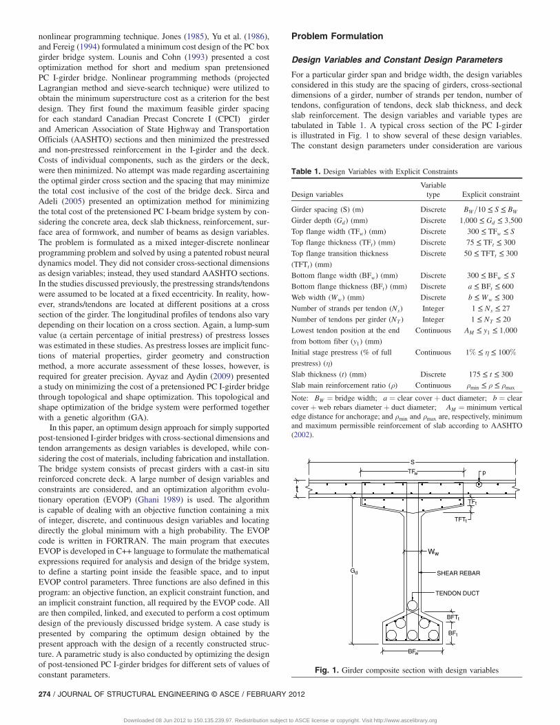
For a particular girder span and bridge width, the design variablesconsidered in this study are the spacing of girders, cross-sectionaldimensions of a girder, number of strands per tendon, number oftendons, configuration of tendons, deck slab thickness, and deckslab reinforcement. The design variables and variable types aretabulated in Table 1. A typical cross section of the PC I-girderis illustrated in Fig. 1 to show several of these design variables.The constant design parameters under consideration are various

Table 1. Design Variables with Explicit Constraints

Design variablesVariabletype Explicit constraint

Girder spacing (S) (m) Discrete BW=10 ≤ S ≤ BW

Girder depth (Gd) (mm) Discrete 1;000 ≤ Gd ≤ 3;500

Top flange width (TFw) (mm) Discrete 300 ≤ TFw ≤ S

Top flange thickness (TFt) (mm) Discrete 75 ≤ TFt ≤ 300

Top flange transition thickness

(TFTt) (mm)

Discrete 50 ≤ TFTt ≤ 300

Bottom flange width (BFw) (mm) Discrete 300 ≤ BFw ≤ S

Bottom flange thickness (BFt) (mm) Discrete a ≤ BFt ≤ 600

Web width (Ww) (mm) Discrete b ≤ Ww ≤ 300

Number of strands per tendon (Ns) Integer 1 ≤ Ns ≤ 27

Number of tendons per girder (NT ) Integer 1 ≤ NT ≤ 20

Lowest tendon position at the end

from bottom fiber (y1) (mm)

Continuous AM ≤ y1 ≤ 1;000

Initial stage prestress (% of full

prestress) (η)Continuous 1% ≤ η ≤ 100%

Slab thickness (t) (mm) Discrete 175 ≤ t ≤ 300

Slab main reinforcement ratio (ρ) Continuous ρmin ≤ ρ ≤ ρmax

Note: BW ¼ bridge width; a ¼ clear cover þ duct diameter; b ¼ clearcover þ web rebars diameter þ duct diameter; AM ¼ minimum verticaledge distance for anchorage; and ρmin and ρmax are, respectively, minimumand maximum permissible reinforcement of slab according to AASHTO(2002).

BFw

BF

BFT

t

t

TF

S

tTF

TFT

G

Ww

d

t

t

w p

SHEAR REBAR

TENDON DUCT

Fig. 1. Girder composite section with design variables

274 / JOURNAL OF STRUCTURAL ENGINEERING © ASCE / FEBRUARY 2012


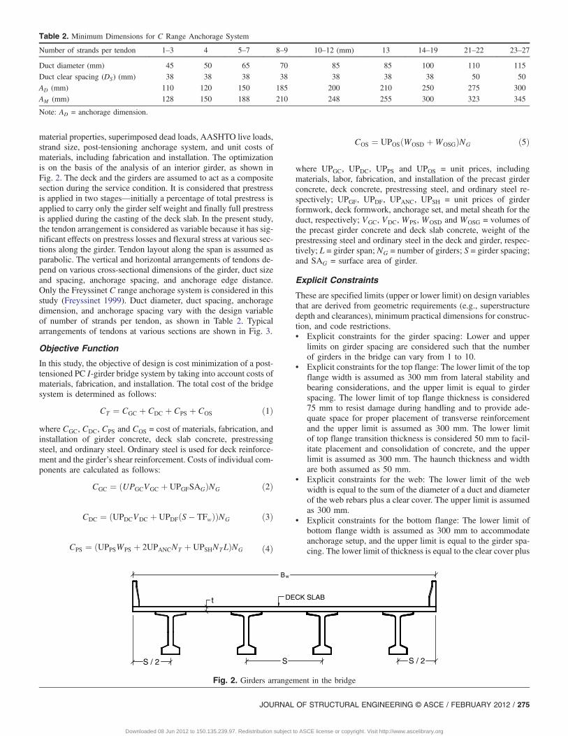
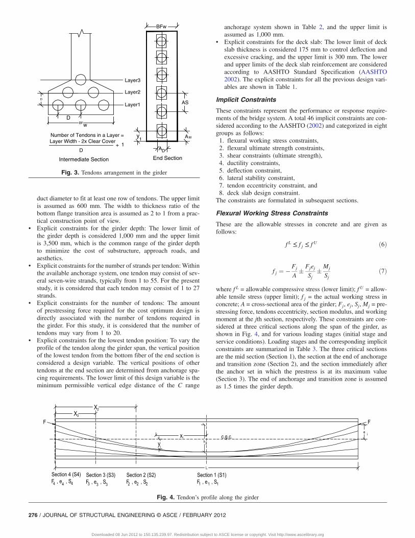
material properties, superimposed dead loads, AASHTO live loads,strand size, post-tensioning anchorage system, and unit costs ofmaterials, including fabrication and installation. The optimizationis on the basis of the analysis of an interior girder, as shown inFig. 2. The deck and the girders are assumed to act as a compositesection during the service condition. It is considered that prestressis applied in two stages—initially a percentage of total prestress isapplied to carry only the girder self weight and finally full prestressis applied during the casting of the deck slab. In the present study,the tendon arrangement is considered as variable because it has sig-nificant effects on prestress losses and flexural stress at various sec-tions along the girder. Tendon layout along the span is assumed asparabolic. The vertical and horizontal arrangements of tendons de-pend on various cross-sectional dimensions of the girder, duct sizeand spacing, anchorage spacing, and anchorage edge distance.Only the Freyssinet C range anchorage system is considered in thisstudy (Freyssinet 1999). Duct diameter, duct spacing, anchoragedimension, and anchorage spacing vary with the design variableof number of strands per tendon, as shown in Table 2. Typicalarrangements of tendons at various sections are shown in Fig. 3.

Objective Function

In this study, the objective of design is cost minimization of a post-tensioned PC I-girder bridge system by taking into account costs ofmaterials, fabrication, and installation. The total cost of the bridgesystem is determined as follows:

CT ¼ CGC þ CDC þ CPS þ COS ð1Þwhere CGC, CDC, CPS and COS = cost of materials, fabrication, andinstallation of girder concrete, deck slab concrete, prestressingsteel, and ordinary steel. Ordinary steel is used for deck reinforce-ment and the girder’s shear reinforcement. Costs of individual com-ponents are calculated as follows:

CGC ¼ ðUPGCVGC þ UPGFSAGÞNG ð2Þ

CDC ¼ ðUPDCVDC þ UPDFðS� TFwÞÞNG ð3Þ

CPS ¼ ðUPPSWPS þ 2UPANCNT þ UPSHNTLÞNG ð4Þ

COS ¼ UPOSðWOSD þWOSGÞNG ð5Þ

where UPGC, UPDC, UPPS and UPOS = unit prices, includingmaterials, labor, fabrication, and installation of the precast girderconcrete, deck concrete, prestressing steel, and ordinary steel re-spectively; UPGF, UPDF, UPANC, UPSH = unit prices of girderformwork, deck formwork, anchorage set, and metal sheath for theduct, respectively; VGC, VDC, WPS, WOSD and WOSG = volumes ofthe precast girder concrete and deck slab concrete, weight of theprestressing steel and ordinary steel in the deck and girder, respec-tively; L = girder span; NG = number of girders; S = girder spacing;and SAG = surface area of girder.

Explicit Constraints

These are specified limits (upper or lower limit) on design variablesthat are derived from geometric requirements (e.g., superstructuredepth and clearances), minimum practical dimensions for construc-tion, and code restrictions.• Explicit constraints for the girder spacing: Lower and upper

limits on girder spacing are considered such that the numberof girders in the bridge can vary from 1 to 10.

• Explicit constraints for the top flange: The lower limit of the topflange width is assumed as 300 mm from lateral stability andbearing considerations, and the upper limit is equal to girderspacing. The lower limit of top flange thickness is considered75 mm to resist damage during handling and to provide ade-quate space for proper placement of transverse reinforcementand the upper limit is assumed as 300 mm. The lower limitof top flange transition thickness is considered 50 mm to facil-itate placement and consolidation of concrete, and the upperlimit is assumed as 300 mm. The haunch thickness and widthare both assumed as 50 mm.

• Explicit constraints for the web: The lower limit of the webwidth is equal to the sum of the diameter of a duct and diameterof the web rebars plus a clear cover. The upper limit is assumedas 300 mm.

• Explicit constraints for the bottom flange: The lower limit ofbottom flange width is assumed as 300 mm to accommodateanchorage setup, and the upper limit is equal to the girder spa-cing. The lower limit of thickness is equal to the clear cover plus

Table 2. Minimum Dimensions for C Range Anchorage System

Number of strands per tendon 1–3 4 5–7 8–9 10–12 (mm) 13 14–19 21–22 23–27

Duct diameter (mm) 45 50 65 70 85 85 100 110 115

Duct clear spacing (DS) (mm) 38 38 38 38 38 38 38 50 50

AD (mm) 110 120 150 185 200 210 250 275 300

AM (mm) 128 150 188 210 248 255 300 323 345

Note: AD = anchorage dimension.

S

Bw

DECK SLABt

S / 2 S / 2

Fig. 2. Girders arrangement in the bridge



duct diameter to fit at least one row of tendons. The upper limitis assumed as 600 mm. The width to thickness ratio of thebottom flange transition area is assumed as 2 to 1 from a prac-tical construction point of view.

• Explicit constraints for the girder depth: The lower limit ofthe girder depth is considered 1,000 mm and the upper limitis 3,500 mm, which is the common range of the girder depthto minimize the cost of substructure, approach roads, andaesthetics.

• Explicit constraints for the number of strands per tendon: Withinthe available anchorage system, one tendon may consist of sev-eral seven-wire strands, typically from 1 to 55. For the presentstudy, it is considered that each tendon may consist of 1 to 27strands.

• Explicit constraints for the number of tendons: The amountof prestressing force required for the cost optimum design isdirectly associated with the number of tendons required inthe girder. For this study, it is considered that the number oftendons may vary from 1 to 20.

• Explicit constraints for the lowest tendon position: To vary theprofile of the tendon along the girder span, the vertical positionof the lowest tendon from the bottom fiber of the end section isconsidered a design variable. The vertical positions of othertendons at the end section are determined from anchorage spa-cing requirements. The lower limit of this design variable is theminimum permissible vertical edge distance of the C range

anchorage system shown in Table 2, and the upper limit isassumed as 1,000 mm.

• Explicit constraints for the deck slab: The lower limit of deckslab thickness is considered 175 mm to control deflection andexcessive cracking, and the upper limit is 300 mm. The lowerand upper limits of the deck slab reinforcement are consideredaccording to AASHTO Standard Specification (AASHTO2002). The explicit constraints for all the previous design vari-ables are shown in Table 1.

Implicit Constraints

These constraints represent the performance or response require-ments of the bridge system. A total 46 implicit constraints are con-sidered according to the AASHTO (2002) and categorized in eightgroups as follows:1. flexural working stress constraints,2. flexural ultimate strength constraints,3. shear constraints (ultimate strength),4. ductility constraints,5. deflection constraint,6. lateral stability constraint,7. tendon eccentricity constraint, and8. deck slab design constraint.

The constraints are formulated in subsequent sections.

Flexural Working Stress Constraints

These are the allowable stresses in concrete and are given asfollows:

f L ≤ f j ≤ f U ð6Þ

f j ¼ �Fj

A� Fjej

Sj�Mj

Sjð7Þ

where f L = allowable compressive stress (lower limit); f U = allow-able tensile stress (upper limit); f j = the actual working stress inconcrete; A = cross-sectional area of the girder; Fj, ej, Sj, Mj = pre-stressing force, tendons eccentricity, section modulus, and workingmoment at the jth section, respectively. These constraints are con-sidered at three critical sections along the span of the girder, asshown in Fig. 4, and for various loading stages (initial stage andservice conditions). Loading stages and the corresponding implicitconstraints are summarized in Table 3. The three critical sectionsare the mid section (Section 1), the section at the end of anchorageand transition zone (Section 2), and the section immediately afterthe anchor set in which the prestress is at its maximum value(Section 3). The end of anchorage and transition zone is assumedas 1.5 times the girder depth.

Fig. 4. Tendon’s profile along the girder

M

AS

BFw

AD

1

End Section

BFwD

D

Layer2

Layer1

Layer3

Number of Tendons in a Layer = Layer Width - 2x Clear Cover

D+ 1

Intermediate Section

Ay

Fig. 3. Tendons arrangement in the girder



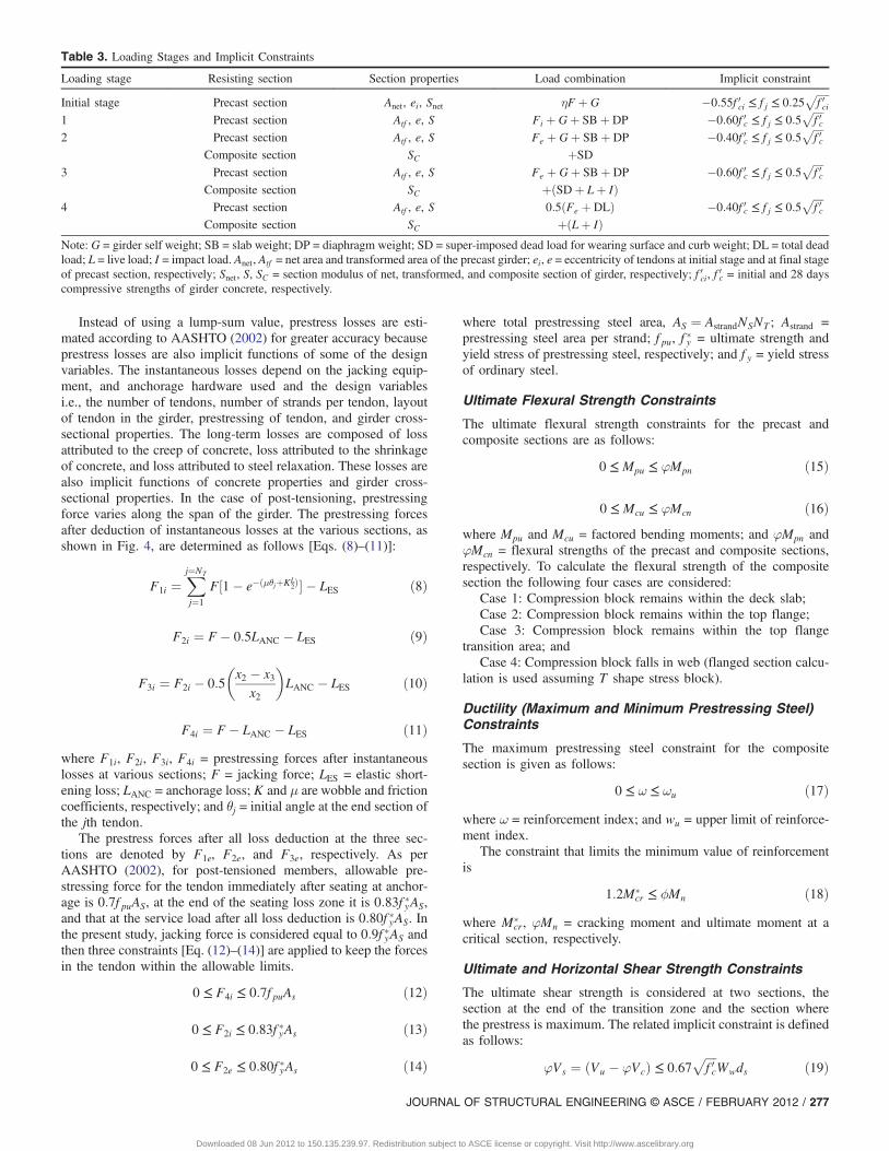
Instead of using a lump-sum value, prestress losses are esti-mated according to AASHTO (2002) for greater accuracy becauseprestress losses are also implicit functions of some of the designvariables. The instantaneous losses depend on the jacking equip-ment, and anchorage hardware used and the design variablesi.e., the number of tendons, number of strands per tendon, layoutof tendon in the girder, prestressing of tendon, and girder cross-sectional properties. The long-term losses are composed of lossattributed to the creep of concrete, loss attributed to the shrinkageof concrete, and loss attributed to steel relaxation. These losses arealso implicit functions of concrete properties and girder cross-sectional properties. In the case of post-tensioning, prestressingforce varies along the span of the girder. The prestressing forcesafter deduction of instantaneous losses at the various sections, asshown in Fig. 4, are determined as follows [Eqs. (8)–(11)]:

F1i ¼Xj¼NT

j¼1

F½1� e�ðμθjþKL2Þ� � LES ð8Þ

F2i ¼ F � 0:5LANC � LES ð9Þ

F3i ¼ F2i � 0:5

�x2 � x3

x2

�LANC � LES ð10Þ

F4i ¼ F � LANC � LES ð11Þwhere F1i, F2i, F3i, F4i = prestressing forces after instantaneouslosses at various sections; F = jacking force; LES = elastic short-ening loss; LANC = anchorage loss; K and μ are wobble and frictioncoefficients, respectively; and θj = initial angle at the end section ofthe jth tendon.

The prestress forces after all loss deduction at the three sec-tions are denoted by F1e, F2e, and F3e, respectively. As perAASHTO (2002), for post-tensioned members, allowable pre-stressing force for the tendon immediately after seating at anchor-age is 0:7f puAS, at the end of the seating loss zone it is 0:83f �yAS,and that at the service load after all loss deduction is 0:80f �yAS. Inthe present study, jacking force is considered equal to 0:9f �yAS andthen three constraints [Eq. (12)–(14)] are applied to keep the forcesin the tendon within the allowable limits.

0 ≤ F4i ≤ 0:7f puAs ð12Þ

0 ≤ F2i ≤ 0:83f �yAs ð13Þ

0 ≤ F2e ≤ 0:80f �yAs ð14Þ

where total prestressing steel area, AS ¼ AstrandNSNT ; Astrand =prestressing steel area per strand; f pu, f �y = ultimate strength andyield stress of prestressing steel, respectively; and f y = yield stressof ordinary steel.

Ultimate Flexural Strength Constraints

The ultimate flexural strength constraints for the precast andcomposite sections are as follows:

0 ≤ Mpu ≤ φMpn ð15Þ

0 ≤ Mcu ≤ φMcn ð16Þwhere Mpu and Mcu = factored bending moments; and φMpn andφMcn = flexural strengths of the precast and composite sections,respectively. To calculate the flexural strength of the compositesection the following four cases are considered:

Case 1: Compression block remains within the deck slab;Case 2: Compression block remains within the top flange;Case 3: Compression block remains within the top flange

transition area; andCase 4: Compression block falls in web (flanged section calcu-

lation is used assuming T shape stress block).

Ductility (Maximum and Minimum Prestressing Steel)Constraints

The maximum prestressing steel constraint for the compositesection is given as follows:

0 ≤ ω ≤ ωu ð17Þwhere ω = reinforcement index; and wu = upper limit of reinforce-ment index.

The constraint that limits the minimum value of reinforcementis

1:2M�cr ≤ ϕMn ð18Þ

where M�cr , φMn = cracking moment and ultimate moment at a

critical section, respectively.

Ultimate and Horizontal Shear Strength Constraints

The ultimate shear strength is considered at two sections, thesection at the end of the transition zone and the section wherethe prestress is maximum. The related implicit constraint is definedas follows:

φVs ¼ ðVu � φVcÞ ≤ 0:67ffiffiffiffif 0c

pWwds ð19Þ

Table 3. Loading Stages and Implicit Constraints

Loading stage Resisting section Section properties Load combination Implicit constraint

Initial stage Precast section Anet, ei, Snet ηF þ G �0:55f 0ci ≤ f j ≤ 0:25ffiffiffiffiffif 0ci

p1 Precast section Atf , e, S Fi þ Gþ SBþ DP �0:60f 0c ≤ f j ≤ 0:5

ffiffiffiffif 0c

p2 Precast section Atf , e, S Fe þ Gþ SBþ DP �0:40f 0c ≤ f j ≤ 0:5

ffiffiffiffif 0c

pComposite section SC þSD

3 Precast section Atf , e, S Fe þ Gþ SBþ DP �0:60f 0c ≤ f j ≤ 0:5ffiffiffiffif 0c

pComposite section SC þðSDþ Lþ IÞ

4 Precast section Atf , e, S 0:5ðFe þ DLÞ �0:40f 0c ≤ f j ≤ 0:5ffiffiffiffif 0c

pComposite section SC þðLþ IÞ

Note: G = girder self weight; SB = slab weight; DP = diaphragm weight; SD = super-imposed dead load for wearing surface and curb weight; DL = total deadload; L = live load; I = impact load. Anet, Atf = net area and transformed area of the precast girder; ei, e = eccentricity of tendons at initial stage and at final stageof precast section, respectively; Snet, S, SC = section modulus of net, transformed, and composite section of girder, respectively; f 0ci, f

0c = initial and 28 days

compressive strengths of girder concrete, respectively.



where Vu = factored shear at a section; Vc = the concrete contri-bution taken as lesser of flexural shear, Vci and web shear, Vcw, inkilonewtons; and Vs = shear carried by the steel in kN. These twoshear capacities are determined according to AASHTO (2002).

The constraint for horizontal shear for composite section is

Vu ≤ φVnh ð20Þwhere Vnh = nominal horizontal shear strength.

Deflection Constraints

Deflection attributed to live load (AISC Marketing 1986) is

ΔLL ¼ 324EcIc

PTðL3 � 555Lþ 4780Þ ð21Þ

where PT = weight of one front wheel multiplied by the distributionfactor plus impact; Ec = modulus of elasticity of girder concrete;and Ic = moment of inertia of the composite girder section.

The live load deflection constraint is

ΔLL ≤ L800

ð22Þ

End Section Tendon Eccentricity Constraint

The constraint that limits the tendon eccentricity at the end sectionso that the extreme fiber tension remains within the allowable limitsis as follows:

Gd

6þ 0:25

ffiffiffiffiffif 0ci

p AendGd

6F4i≤ e4 ≤ Gd

6þ 0:5

ffiffiffiffif 0c

p AendGd

6F4eð23Þ

where Aend = cross-sectional area of the end section of the girder.

Lateral Stability Constraint

The following constraint, according to PCI (2003), ensures thesafety and stability during the lifting of a long girder, subject toroll about the weak axis

FSC ≥ 1:5 ð24Þwhere FSc = factor of safety against cracking of top flange when thegirder hangs from the lifting loop.

Deck Slab Constraints

The constraint considered for deck slab thickness according to thedesign criteria of ODOT (2000) is

t ≥ Sd þ 173

ð25Þ

The constraint that limits the required effective depth for deckslab is

dmin ≤ dreq ≤ dprov ð26Þwhere Sd = effective slab span in feet = S� TFw=2; t = slabthickness in inches; and dreq, dprov, dmin = required, providedand minimum effective depth of deck slab, respectively.

Optimization Method

The bridge optimization problem under discussion is characterizedby a large number of design variables and constraints. The designvariables are a combination of continuous, discrete, and integertypes. Expressions for the objective function and the constraints

are nonlinear functions of these design variables. The optimal de-sign problem, therefore, becomes highly nonlinear and nonconvex,having multiple local minimums that require a method capable oflocating the global optimum by handling mixed integer, discrete,and continuous arguments.

The procedure EVOP has successfully minimized a large num-ber of recognized test problems (Ghani 1989, 1995). An updatedversion of EVOP is used in this study that is capable of minimizingobjective functions having a combination of integer, discrete, andcontinuous arguments as well. The method treats all arguments ascontinuous, but for discrete and integer design variables, themethod picks values from within thin strips centered on specifiedvalues. A Users’ Manual for EVOP with several test examples canbe found in Ghani (2008).

The algorithm can minimize an objective function

f 0ðxÞ ¼ f 0ðx1; x2…xnÞ ð27Þwhere f 0ðxÞ = function of n independent variablesxT ¼ ðx1; x2…xnÞ.

The n independent variables xi‘s ði ¼ 1; 2…:nÞ are subject toexplicit constraints

li ≤ xi ≤ ui ð28Þwhere li‘s and ui‘s = lower and upper limits on the variables, re-spectively. They are either constants or functions of n independentvariables (moving boundaries). These explicit constraints must de-fine, at best, a convex or, at worst, a semiconvex n-dimensionalvector-space but never a nonconvex vector-space. Any explicit con-straint that renders the vector-space nonconvex should be classifiedas an implicit constraint discussed subsequently and shifted to theimplicit constraint set. The corresponding variable, however,should be given a fixed upper and a lower limit and included inthe explicit constraint set, thus, rendering the vector-space definedby only the explicit constraints to become semiconvex.

These n independent variables xi‘s are also subject tom numbersof implicit constraints

Lj ≤ f jðx1; x2…xnÞ ≤ Uj ð29Þ

where j ¼ 1; 2…:m; and Lj‘s and Uj‘s = lower and upper limits onthe m implicit constraints, respectively. They are either constants orfunctions of the n independent variables. The implicit constraintsare allowed to make the feasible vector-space nonconvex.

Additionally, the optimization may also be subject to k numbersof equality constraints of the form

hjðxÞ ¼ 0 where j ¼ 1; 2…; k ð30Þ

Functions hjðxÞ are also of arbitrary complexity of n indepen-dent variables ðx1; x2;……:; xnÞ. The procedure is unable todirectly deal with the previous form of equality constraints. It, how-ever, can indirectly handle such equality constraints by defining anaugmented objective function

Fðx;λÞ ¼ f 0ðxÞ þ ΣλjhjðxÞ ð31Þ

where j ¼ 1;………; k; and λj‘s = unknown weighting factors suchthat all hjðxÞ vanish at the minimum of Fðx;λÞ.

In the literature, λj‘s are known as Lagrange multipliers.The previous problem needs to be presented to the subroutine

EVOP as follows:

MinimizeFðx;λÞ ¼ f 0ðxÞ þ ΣλjhjðxÞ where j ¼ 1;………:; k

ð32Þ



Subject to explicit constraints li ≤ xi ≤ uii ¼ 1;………:; n Eq. (28)repeated

and 0 ≤ λj ≤ any positive number j ¼ 1;………:; k ð33Þand an additional set of k numbers of implicit constraints

0 ≤ hjðxÞ ≤ any positive number greater than hjðx0Þ ð34Þwhere x0 = starting point.

If the numerical value of hjðxÞ is negative, then either negatehjðxÞ to make it positive or just square it.

Procedure

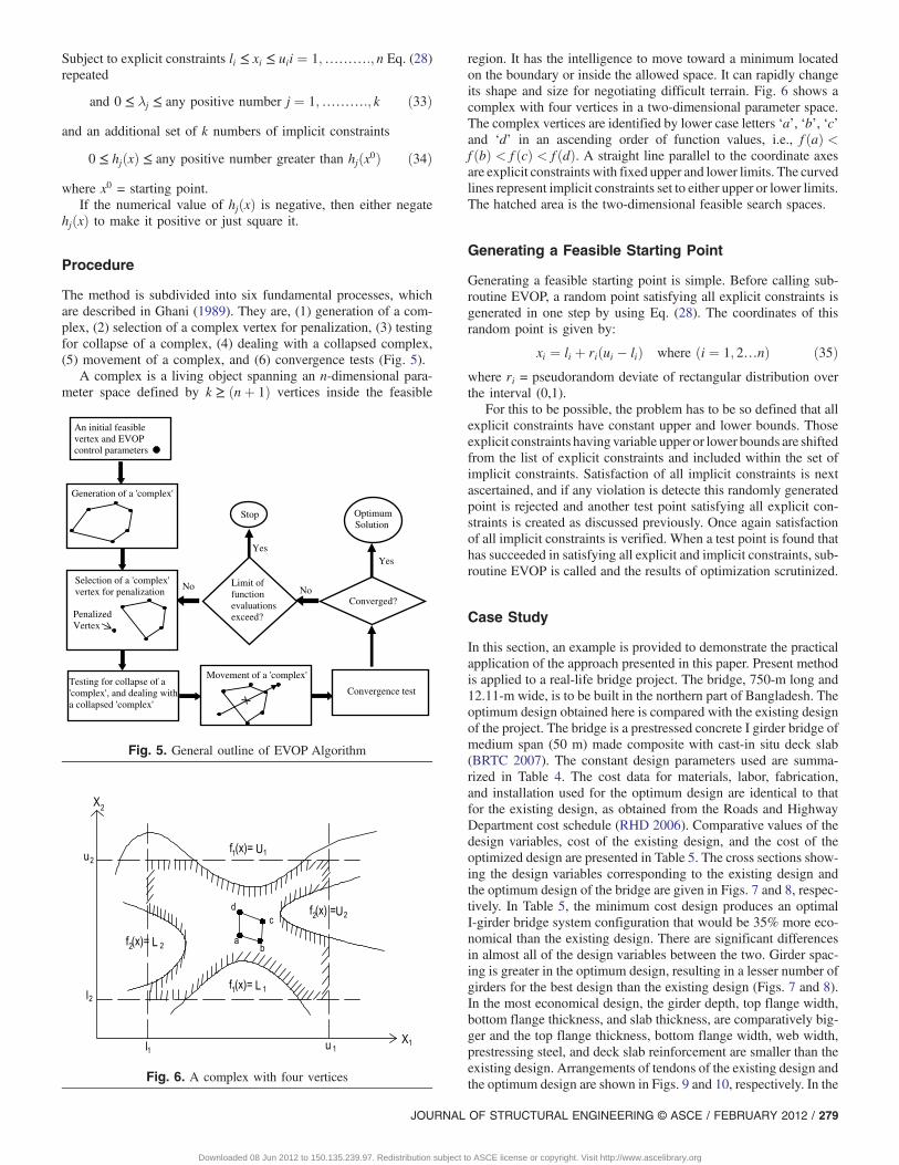
The method is subdivided into six fundamental processes, whichare described in Ghani (1989). They are, (1) generation of a com-plex, (2) selection of a complex vertex for penalization, (3) testingfor collapse of a complex, (4) dealing with a collapsed complex,(5) movement of a complex, and (6) convergence tests (Fig. 5).

A complex is a living object spanning an n-dimensional para-meter space defined by k ≥ ðnþ 1Þ vertices inside the feasible

region. It has the intelligence to move toward a minimum locatedon the boundary or inside the allowed space. It can rapidly changeits shape and size for negotiating difficult terrain. Fig. 6 shows acomplex with four vertices in a two-dimensional parameter space.The complex vertices are identified by lower case letters ‘a’, ‘b’, ‘c’and ‘d’ in an ascending order of function values, i.e., f ðaÞ <f ðbÞ < f ðcÞ < f ðdÞ. A straight line parallel to the coordinate axesare explicit constraints with fixed upper and lower limits. The curvedlines represent implicit constraints set to either upper or lower limits.The hatched area is the two-dimensional feasible search spaces.

Generating a Feasible Starting Point

Generating a feasible starting point is simple. Before calling sub-routine EVOP, a random point satisfying all explicit constraints isgenerated in one step by using Eq. (28). The coordinates of thisrandom point is given by:

xi ¼ li þ riðui � liÞ where ði ¼ 1; 2…nÞ ð35Þwhere ri = pseudorandom deviate of rectangular distribution overthe interval (0,1).

For this to be possible, the problem has to be so defined that allexplicit constraints have constant upper and lower bounds. Thoseexplicit constraints having variable upper or lower bounds are shiftedfrom the list of explicit constraints and included within the set ofimplicit constraints. Satisfaction of all implicit constraints is nextascertained, and if any violation is detecte this randomly generatedpoint is rejected and another test point satisfying all explicit con-straints is created as discussed previously. Once again satisfactionof all implicit constraints is verified. When a test point is found thathas succeeded in satisfying all explicit and implicit constraints, sub-routine EVOP is called and the results of optimization scrutinized.

Case Study

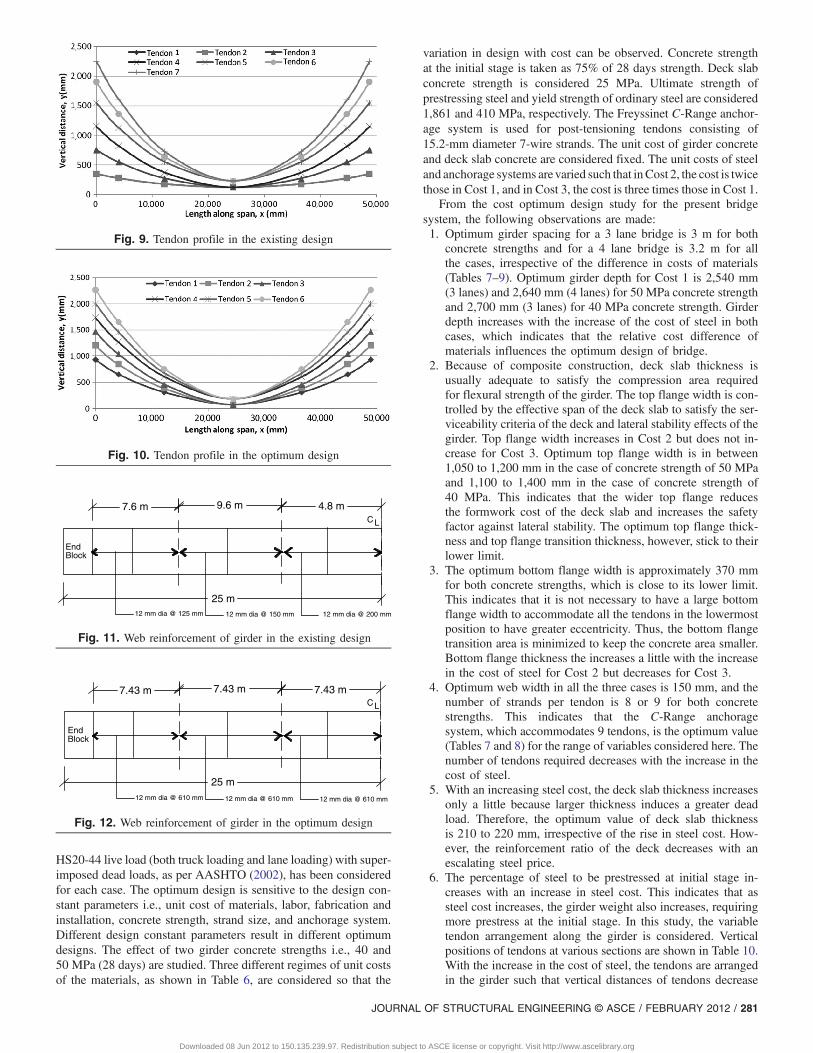
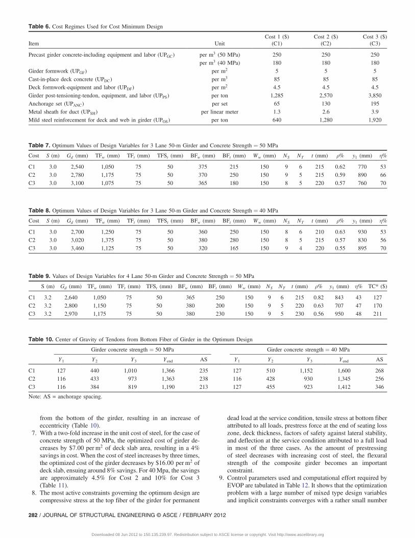
In this section, an example is provided to demonstrate the practicalapplication of the approach presented in this paper. Present methodis applied to a real-life bridge project. The bridge, 750-m long and12.11-m wide, is to be built in the northern part of Bangladesh. Theoptimum design obtained here is compared with the existing designof the project. The bridge is a prestressed concrete I girder bridge ofmedium span (50 m) made composite with cast-in situ deck slab(BRTC 2007). The constant design parameters used are summa-rized in Table 4. The cost data for materials, labor, fabrication,and installation used for the optimum design are identical to thatfor the existing design, as obtained from the Roads and HighwayDepartment cost schedule (RHD 2006). Comparative values of thedesign variables, cost of the existing design, and the cost of theoptimized design are presented in Table 5. The cross sections show-ing the design variables corresponding to the existing design andthe optimum design of the bridge are given in Figs. 7 and 8, respec-tively. In Table 5, the minimum cost design produces an optimalI-girder bridge system configuration that would be 35% more eco-nomical than the existing design. There are significant differencesin almost all of the design variables between the two. Girder spac-ing is greater in the optimum design, resulting in a lesser number ofgirders for the best design than the existing design (Figs. 7 and 8).In the most economical design, the girder depth, top flange width,bottom flange thickness, and slab thickness, are comparatively big-ger and the top flange thickness, bottom flange width, web width,prestressing steel, and deck slab reinforcement are smaller than theexisting design. Arrangements of tendons of the existing design andthe optimum design are shown in Figs. 9 and 10, respectively. In the

No No

Yes

Testing for collapse of a 'complex', and dealing with a collapsed 'complex'

Convergence test

Movement of a 'complex'

Generation of a 'complex'

Selection of a 'complex' vertex for penalization

Penalized Vertex

An initial feasible vertex and EVOP control parameters

Limit of function evaluations exceed?

Stop OptimumSolution

Yes

Converged?

Fig. 5. General outline of EVOP Algorithm

Fig. 6. A complex with four vertices



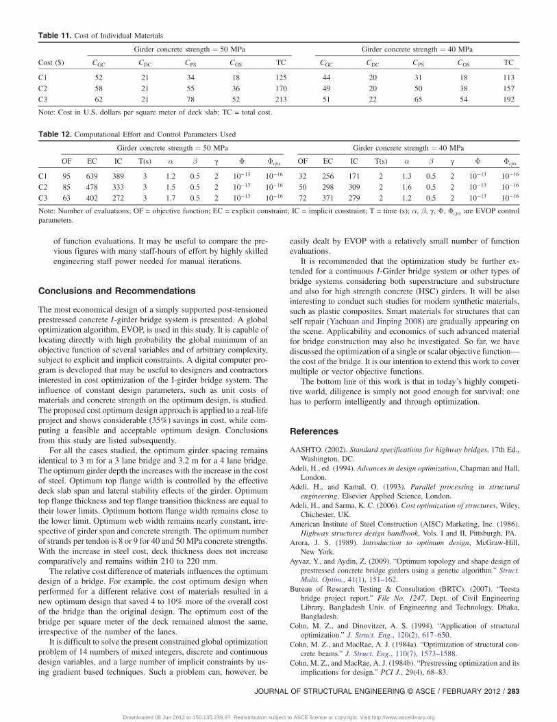
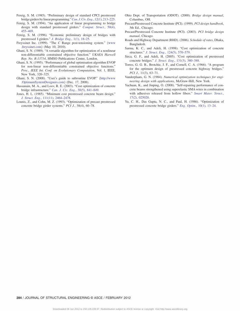
optimum design, tendon arrangement is steeper than that of theexisting design. This indicates that consideration of tendon arrange-ment as a design variable is important because it affects, to a greatextent, the prestress losses and flexural stress at various sectionsalong the girder. Web reinforcement of the girder is also less in theoptimum design than that of the existing design (Figs. 11 and 12).The optimization problem with 14 mixed type design variables and46 implicit constraints converges with just 32 numbers of objectivefunction evaluations with 3 digit accuracy. The correspondingnumbers of explicit and implicit constraints evaluations are 256 and171, respectively. An Intel COREi3 processor has been used in thisstudy, and computational time required for optimization by EVOPis around only 2 s. Further, the design process becomes fully auto-mated, making costly expert human involvement unnecessary.

Parametric Study

The present cost optimum design method has been applied for 3lane and 4 lane bridges of a 50 m girder span. The AASHTO

Table 4. Constant Design Parameters

Cost data Material properties Bridge design data

UPGC ¼ $180 per m3 f pu ¼ 1;861 MPa Girder length ¼ 50 m (L ¼ 48:8 m)

UPGF ¼ $5 per m2 f y ¼ 410 MPa Bridge width, BW ¼ 12:0 m (3 lane)

UPDC ¼ $85 per m3 f 0c ¼ 40 MPa Live load = HS20-44 (both truck loading and lane loading)

UPDF ¼ $4:5 per m2 f 0cd ¼ 25 MPa No of diaphragm ¼ 4; diaphragm width ¼ 250 mm

UPPS ¼ $1;285 per t f 0ci ¼ 30 MPa Wearing surface ¼ 50 mm

UPANC ¼ $65 per set K ¼ 0:005=m Curb height ¼ 600 mm; curb width ¼ 450 mm

UPSH ¼ $1:3 per linear m μ ¼ 0:25 7 wire low-relaxation strand

UPOS ¼ $640 per t δ ¼ 6 mm Freyssinet anchorage system

Note: f 0cd = compressive strength of slab concrete.

Table 5. Existing Design and Cost Optimum Design

Design Variables Existingdesign

Optimumdesign

Girder spacing (S) (m) 2.4 3.0

Girder depth (Gd) (mm) 2,500 2,700

Top flange width (TFw) (mm) 1,060 1,250

Top flange thickness (TFt) (mm) 130 75

Top flange transition thickness (mm) 75 50

Web width (Ww) (mm) 220 150

Bottom flange width (BFw) (mm) 710 360

Bottom flange thickness (BFt) (mm) 200 250

Number of strands per tendon (Ns) 12 (0.5″dia) 8 (0.6″dia)Number of tendons per girder (NT ) 7 6

Lowest tendon position (y1) 400 930

Initial stage prestress (η) 42.8% 53%

Slab thickness (t) (mm) 187.5 210

Slab main reinforcement ratio (ρ) 0.82% 0.63%

Other cross-sectional parameters Existing

design

Optimum

design

Top flange transition width (mm) 270 500

Top flange haunch width (mm) 150 50

Top flange haunch thickness (mm) 150 50

Bottom flange transition width (mm) 245 105

Bottom flange transition thickness (mm) 250 52.5

Total cost per square meter of deck ($) 175 113

%SAVING ¼ ½ð175� 113Þ=175 × 100� 35.0%

710

200

250

245

130

150

1,0502,400

2,500

130

7 Tendon12.7 mm dia-12 Strand

per Tendon

187

220

270150

75

Fig. 7. The existing design (dimensions are in millimeters)

360

250

52105

50

50

1,250

2,700

150

6 Tendon15.2 mm dia-8 Strand

per Tendon

210

75

3,000

500

Fig. 8. The optimum design obtained in this study (dimensions are inmillimeters)



HS20-44 live load (both truck loading and lane loading) with super-imposed dead loads, as per AASHTO (2002), has been consideredfor each case. The optimum design is sensitive to the design con-stant parameters i.e., unit cost of materials, labor, fabrication andinstallation, concrete strength, strand size, and anchorage system.Different design constant parameters result in different optimumdesigns. The effect of two girder concrete strengths i.e., 40 and50 MPa (28 days) are studied. Three different regimes of unit costsof the materials, as shown in Table 6, are considered so that the

variation in design with cost can be observed. Concrete strengthat the initial stage is taken as 75% of 28 days strength. Deck slabconcrete strength is considered 25 MPa. Ultimate strength ofprestressing steel and yield strength of ordinary steel are considered1,861 and 410 MPa, respectively. The Freyssinet C-Range anchor-age system is used for post-tensioning tendons consisting of15.2-mm diameter 7-wire strands. The unit cost of girder concreteand deck slab concrete are considered fixed. The unit costs of steeland anchorage systems arevaried such that inCost 2, the cost is twicethose in Cost 1, and in Cost 3, the cost is three times those in Cost 1.

From the cost optimum design study for the present bridgesystem, the following observations are made:1. Optimum girder spacing for a 3 lane bridge is 3 m for both

concrete strengths and for a 4 lane bridge is 3.2 m for allthe cases, irrespective of the difference in costs of materials(Tables 7–9). Optimum girder depth for Cost 1 is 2,540 mm(3 lanes) and 2,640 mm (4 lanes) for 50 MPa concrete strengthand 2,700 mm (3 lanes) for 40 MPa concrete strength. Girderdepth increases with the increase of the cost of steel in bothcases, which indicates that the relative cost difference ofmaterials influences the optimum design of bridge.

2. Because of composite construction, deck slab thickness isusually adequate to satisfy the compression area requiredfor flexural strength of the girder. The top flange width is con-trolled by the effective span of the deck slab to satisfy the ser-viceability criteria of the deck and lateral stability effects of thegirder. Top flange width increases in Cost 2 but does not in-crease for Cost 3. Optimum top flange width is in between1,050 to 1,200 mm in the case of concrete strength of 50 MPaand 1,100 to 1,400 mm in the case of concrete strength of40 MPa. This indicates that the wider top flange reducesthe formwork cost of the deck slab and increases the safetyfactor against lateral stability. The optimum top flange thick-ness and top flange transition thickness, however, stick to theirlower limit.

3. The optimum bottom flange width is approximately 370 mmfor both concrete strengths, which is close to its lower limit.This indicates that it is not necessary to have a large bottomflange width to accommodate all the tendons in the lowermostposition to have greater eccentricity. Thus, the bottom flangetransition area is minimized to keep the concrete area smaller.Bottom flange thickness the increases a little with the increasein the cost of steel for Cost 2 but decreases for Cost 3.

4. Optimum web width in all the three cases is 150 mm, and thenumber of strands per tendon is 8 or 9 for both concretestrengths. This indicates that the C-Range anchoragesystem, which accommodates 9 tendons, is the optimum value(Tables 7 and 8) for the range of variables considered here. Thenumber of tendons required decreases with the increase in thecost of steel.

5. With an increasing steel cost, the deck slab thickness increasesonly a little because larger thickness induces a greater deadload. Therefore, the optimum value of deck slab thicknessis 210 to 220 mm, irrespective of the rise in steel cost. How-ever, the reinforcement ratio of the deck decreases with anescalating steel price.

6. The percentage of steel to be prestressed at initial stage in-creases with an increase in steel cost. This indicates that assteel cost increases, the girder weight also increases, requiringmore prestress at the initial stage. In this study, the variabletendon arrangement along the girder is considered. Verticalpositions of tendons at various sections are shown in Table 10.With the increase in the cost of steel, the tendons are arrangedin the girder such that vertical distances of tendons decrease

Fig. 9. Tendon profile in the existing design

Fig. 10. Tendon profile in the optimum design

C L

EndBlock

7.6 m 9.6 m 4.8 m

25 m12 mm dia @ 125 mm 12 mm dia @ 150 mm 12 mm dia @ 200 mm

Fig. 11. Web reinforcement of girder in the existing design

12 mm dia @ 610 mm 12 mm dia @ 610 mm 12 mm dia @ 610 mm

CL

EndBlock

7.43 m 7.43 m 7.43 m

25 m

Fig. 12. Web reinforcement of girder in the optimum design



from the bottom of the girder, resulting in an increase ofeccentricity (Table 10).

7. With a two-fold increase in the unit cost of steel, for the case ofconcrete strength of 50 MPa, the optimized cost of girder de-creases by $7:00 per m2 of deck slab area, resulting in a 4%savings in cost. When the cost of steel increases by three times,the optimized cost of the girder decreases by $16:00 per m2 ofdeck slab, ensuing around 8% savings. For 40Mpa, the savingsare approximately 4.5% for Cost 2 and 10% for Cost 3(Table 11).

8. The most active constraints governing the optimum design arecompressive stress at the top fiber of the girder for permanent

dead load at the service condition, tensile stress at bottom fiberattributed to all loads, prestress force at the end of seating losszone, deck thickness, factors of safety against lateral stability,and deflection at the service condition attributed to a full loadin most of the three cases. As the amount of prestressingof steel decreases with increasing cost of steel, the flexuralstrength of the composite girder becomes an importantconstraint.

9. Control parameters used and computational effort required byEVOP are tabulated in Table 12. It shows that the optimizationproblem with a large number of mixed type design variablesand implicit constraints converges with a rather small number

Table 6. Cost Regimes Used for Cost Minimum Design

Item UnitCost 1 ($)

(C1)Cost 2 ($)

(C2)Cost 3 ($)

(C3)

Precast girder concrete-including equipment and labor (UPGC) per m3 (50 MPa) 250 250 250

per m3 (40 MPa) 180 180 180

Girder formwork (UPGF) per m2 5 5 5

Cast-in-place deck concrete (UPDC) per m3 85 85 85

Deck formwork-equipment and labor (UPDF) per m2 4.5 4.5 4.5

Girder post-tensioning-tendon, equipment, and labor (UPPS) per ton 1,285 2,570 3,850

Anchorage set (UPANC) per set 65 130 195

Metal sheath for duct (UPSH) per linear meter 1.3 2.6 3.9

Mild steel reinforcement for deck and web in girder (UPOS) per ton 640 1,280 1,920

Table 7. Optimum Values of Design Variables for 3 Lane 50-m Girder and Concrete Strength ¼ 50 MPa

Cost S (m) Gd (mm) TFw (mm) TFt (mm) TFSt (mm) BFw (mm) BFt (mm) Ww (mm) NS NT t (mm) ρ% y1 (mm) η%

C1 3.0 2,540 1,050 75 50 375 215 150 9 6 215 0.62 770 53

C2 3.0 2,780 1,175 75 50 370 250 150 9 5 215 0.59 890 66

C3 3.0 3,100 1,075 75 50 365 180 150 8 5 220 0.57 760 70

Table 8. Optimum Values of Design Variables for 3 Lane 50-m Girder and Concrete Strength ¼ 40 MPa

Cost S (m) Gd (mm) TFw (mm) TFt (mm) TFSt (mm) BFw (mm) BFt (mm) Ww (mm) NS NT t (mm) ρ% y1 (mm) η%

C1 3.0 2,700 1,250 75 50 360 250 150 8 6 210 0.63 930 53

C2 3.0 3,020 1,375 75 50 380 280 150 8 5 215 0.57 830 56

C3 3.0 3,460 1,125 75 50 320 165 150 9 4 220 0.55 895 70

Table 9. Values of Design Variables for 4 Lane 50-m Girder and Concrete Strength ¼ 50 MPa

S (m) Gd (mm) TFw (mm) TFt (mm) TFSt (mm) BFw (mm) BFt (mm) Ww (mm) NS NT t (mm) ρ% y1 (mm) η% TC* ($)

C1 3.2 2,640 1,050 75 50 365 250 150 9 6 215 0.82 843 43 127

C2 3.2 2,800 1,150 75 50 380 200 150 9 5 220 0.63 707 47 170

C3 3.2 2,970 1,175 75 50 380 230 150 9 5 230 0.56 950 48 211

Table 10. Center of Gravity of Tendons from Bottom Fiber of Girder in the Optimum Design

Girder concrete strength ¼ 50 MPa Girder concrete strength ¼ 40 MPa

Y1 Y2 Y3 Yend AS Y1 Y2 Y3 Yend AS

C1 127 440 1,010 1,366 235 127 510 1,152 1,600 268

C2 116 433 973 1,363 238 116 428 930 1,345 256

C3 116 384 819 1,190 213 127 455 923 1,412 346

Note: AS = anchorage spacing.



of function evaluations. It may be useful to compare the pre-vious figures with many staff-hours of effort by highly skilledengineering staff power needed for manual iterations.

Conclusions and Recommendations

The most economical design of a simply supported post-tensionedprestressed concrete I-girder bridge system is presented. A globaloptimization algorithm, EVOP, is used in this study. It is capable oflocating directly with high probability the global minimum of anobjective function of several variables and of arbitrary complexity,subject to explicit and implicit constraints. A digital computer pro-gram is developed that may be useful to designers and contractorsinterested in cost optimization of the I-girder bridge system. Theinfluence of constant design parameters, such as unit costs ofmaterials and concrete strength on the optimum design, is studied.The proposed cost optimum design approach is applied to a real-lifeproject and shows considerable (35%) savings in cost, while com-puting a feasible and acceptable optimum design. Conclusionsfrom this study are listed subsequently.

For all the cases studied, the optimum girder spacing remainsidentical to 3 m for a 3 lane bridge and 3.2 m for a 4 lane bridge.The optimum girder depth the increases with the increase in the costof steel. Optimum top flange width is controlled by the effectivedeck slab span and lateral stability effects of the girder. Optimumtop flange thickness and top flange transition thickness are equal totheir lower limits. Optimum bottom flange width remains close tothe lower limit. Optimum web width remains nearly constant, irre-spective of girder span and concrete strength. The optimum numberof strands per tendon is 8 or 9 for 40 and 50MPa concrete strengths.With the increase in steel cost, deck thickness does not increasecomparatively and remains within 210 to 220 mm.

The relative cost difference of materials influences the optimumdesign of a bridge. For example, the cost optimum design whenperformed for a different relative cost of materials resulted in anew optimum design that saved 4 to 10% more of the overall costof the bridge than the original design. The optimum cost of thebridge per square meter of the deck remained almost the same,irrespective of the number of the lanes.

It is difficult to solve the present constrained global optimizationproblem of 14 numbers of mixed integers, discrete and continuousdesign variables, and a large number of implicit constraints by us-ing gradient based techniques. Such a problem can, however, be

easily dealt by EVOP with a relatively small number of functionevaluations.

It is recommended that the optimization study be further ex-tended for a continuous I-Girder bridge system or other types ofbridge systems considering both superstructure and substructureand also for high strength concrete (HSC) girders. It will be alsointeresting to conduct such studies for modern synthetic materials,such as plastic composites. Smart materials for structures that canself repair (Yachuan and Jinping 2008) are gradually appearing onthe scene. Applicability and economics of such advanced materialfor bridge construction may also be investigated. So far, we havediscussed the optimization of a single or scalar objective function—the cost of the bridge. It is our intention to extend this work to covermultiple or vector objective functions.

The bottom line of this work is that in today’s highly competi-tive world, diligence is simply not good enough for survival; onehas to perform intelligently and through optimization.

References

AASHTO. (2002). Standard specifications for highway bridges, 17th Ed.,Washington, DC.

Adeli, H., ed. (1994). Advances in design optimization, Chapman and Hall,London.

Adeli, H., and Kamal, O. (1993). Parallel processing in structuralengineering, Elsevier Applied Science, London.

Adeli, H., and Sarma, K. C. (2006). Cost optimization of structures, Wiley,Chichester, UK.

American Institute of Steel Construction (AISC) Marketing, Inc. (1986).Highway structures design handbook, Vols. I and II, Pittsburgh, PA.

Arora, J. S. (1989). Introduction to optimum design, McGraw-Hill,New York.

Ayvaz, Y., and Aydin, Z. (2009). “Optimum topology and shape design ofprestressed concrete bridge girders using a genetic algorithm.” Struct.Multi. Optim., 41(1), 151–162.

Bureau of Research Testing & Consultation (BRTC). (2007). “Teestabridge project report.” File No. 1247, Dept. of Civil EngineeringLibrary, Bangladesh Univ. of Engineering and Technology, Dhaka,Bangladesh.

Cohn, M. Z., and Dinovitzer, A. S. (1994). “Application of structuraloptimization.” J. Struct. Eng., 120(2), 617–650.

Cohn, M. Z., and MacRae, A. J. (1984a). “Optimization of structural con-crete beams.” J. Struct. Eng., 110(7), 1573–1588.

Cohn, M. Z., and MacRae, A. J. (1984b). “Prestressing optimization and itsimplications for design.” PCI J., 29(4), 68–83.

Table 11. Cost of Individual Materials


Cost ($) CGC CDC CPS COS TC CGC CDC CPS COS TC

C1 52 21 34 18 125 44 20 31 18 113

C2 58 21 55 36 170 49 20 50 38 157

C3 62 21 78 52 213 51 22 65 54 192

Note: Cost in U.S. dollars per square meter of deck slab; TC = total cost.

Table 12. Computational Effort and Control Parameters Used


OF EC IC T(s) α β γ Φ Φcpx OF EC IC T(s) α β γ Φ Φcpx

C1 95 639 389 3 1.2 0.5 2 10�13 10�16 32 256 171 2 1.3 0.5 2 10�13 10�16

C2 85 478 333 3 1.5 0.5 2 10�13 10�16 50 298 309 2 1.6 0.5 2 10�13 10�16

C3 63 402 272 3 1.7 0.5 2 10�13 10�16 72 371 279 2 1.2 0.5 2 10�13 10�16

Note: Number of evaluations; OF = objective function; EC = explicit constraint; IC = implicit constraint; T = time (s); α, β, γ, Φ, Φcpx are EVOP controlparameters.



http://dx.doi.org/10.1007/s00158-009-0404-2

http://dx.doi.org/10.1007/s00158-009-0404-2

http://dx.doi.org/10.1061/(ASCE)0733-9445(1994)120:2(617)


Fereig, S. M. (1985). “Preliminary design of standard CPCI prestressedbridgegirdersby linear programming.”Can. J.Civ.Eng., 12(1),213–225.

Fereig, S. M. (1994). “An application of linear programming to bridgedesign with standard prestressed girders.” Comput. Struct., 50(4),455–469.

Fereig, S. M. (1996). “Economic preliminary design of bridges withprestressed I-girders.” J. Bridge Eng., 1(1), 18–25.

Freyssinet Inc. (1999). “The C Range post-tensioning system.” ⟨www.freyssinet.com⟩ (May 10, 2010).

Ghani, S. N. (1989). “A versatile algorithm for optimization of a nonlinearnon-differentiable constrained objective function.” UKAEA HarwellRep. No. R-13714, HMSO Publications Centre, London.

Ghani, S. N. (1995). “Performance of global optimisation algorithm EVOPfor non-linear non-differentiable constrained objective functions.”Proc., IEEE Int. Conf. on Evolutionary Computation, Vol. 1, IEEE,New York, 320–325.

Ghani, S. N. (2008). “User’s guide to subroutine EVOP.” ⟨http://www.OptimumSystemDesigners.com⟩ (Dec. 17, 2008).

Hassanain, M. A., and Loov, R. E. (2003). “Cost optimization of concretebridge infrastructure.” Can. J. Civ. Eng., 30(5), 841–849.

Jones, H. L. (1985). “Minimum cost prestressed concrete beam design.”J. Struct. Eng., 111(11), 2464–2478.

Lounis, Z., and Cohn, M. Z. (1993). “Optimization of precast prestressedconcrete bridge girder systems.” PCI J., 38(4), 60–78.

Ohio Dept. of Transportation (ODOT). (2000). Bridge design manual,Columbus, OH.

Precast/Prestressed Concrete Institute (PCI). (1999). PCI design handbook,5th Ed., Chicago.

Precast/Prestressed Concrete Institute (PCI). (2003). PCI bridge designmanual, Chicago.

Roads and Highway Department (RHD). (2006). Schedule of rates, Dhaka,Bangladesh.

Sarma, K. C., and Adeli, H. (1998). “Cost optimization of concretestructures.” J. Struct. Eng., 124(5), 570–579.

Sirca, G. F., and Adeli, H. (2005). “Cost optimization of prestressedconcrete bridges.” J. Struct. Eng., 131(3), 380–388.

Torres, G. G. B., Brotchie, J. F., and Cornell, C. A. (1966). “A programfor the optimum design of prestressed concrete highway bridges.”PCI J., 11(3), 63–71.

Vanderplaats, G. N. (1984). Numerical optimization techniques for engi-neering design with applications, McGraw-Hill, New York.

Yachuan, K., and Jinping, O. (2008). “Self-repairing performance of con-crete beams strengthened using superelastic SMAwires in combinationwith adhesives released from hollow fibers.” Smart Mater. Struct.,17(2), 025020.

Yu, C. H., Das Gupta, N. C., and Paul, H. (1986). “Optimization ofprestressed concrete bridge girders.” Eng. Optim., 10(1), 13–24.



http://dx.doi.org/10.1139/l85-020

http://dx.doi.org/10.1016/0045-7949(94)90016-7

http://dx.doi.org/10.1016/0045-7949(94)90016-7


http://www.freyssinet.com



http://www.OptimumSystemDesigners.com



http://dx.doi.org/10.1139/l03-045




http://dx.doi.org/10.1088/0964-1726/17/2/025020

http://dx.doi.org/10.1088/0964-1726/17/2/025020

http://dx.doi.org/10.1080/03052158608902524

Documents

Cost Optimum Design of Posttensioned I-Girder Bridge … · Cost Optimum Design of Posttensioned I-Girder Bridge Using Global Optimization Algorithm Raquib Ahsan1; Shohel Rana2; and