Embed Size (px)
Citation preview

Cost of CapitalEstimation and ApplicationsSECOND EDITION
Shannon P. Pratt, CFA, FASA, MCBA
JOHN WILEY & SONS, INC.


Cost of Capital
3953 P-00 8/29/02 2:41 PM Page i
Critical Praise forCost of Capital: Estimation and Applications, Second Edition
“Good job on enhancing an already great book.”James R. HitchnerPhillips Hitchner Group, Inc.Atlanta, GA
The research using Pratt’s Stats™ database on the size effect “will be most helpfulfor the readers. . . . The discussion of how these studies can get one from where thestudies leave off to the smaller valuation target is great.”
Ronald L. SeigneurSeigneur & Company, P.C., CPAsLakewood, CO
“Many of us have been anxiously awaiting [the] second edition . . . Cost of capitalprocedures are a frequent source of major logical errors, not just judgment errors.Mistakes of this type can leave the decision maker vulnerable, inasmuch as he orshe can actually be proven wrong. This is an area where practitioners badly need aguide such as Cost of Capital, so they understand what they are doing.”
Roger G. IbbotsonIbbotson AssociatesChicago, IL
Other Wiley books by Shannon P. Pratt include:
Cost of Capital WorkbookBusiness Valuation Body of Knowledge: Exam Review and Professional
Reference, Second EditionBusiness Valuation Body of Knowledge WorkbookThe Market Approach to Valuing BusinessesBusiness Valuation Discounts and Premiums
3953 P-00 8/29/02 2:41 PM Page ii
Cost of CapitalEstimation and ApplicationsSECOND EDITION
Shannon P. Pratt, CFA, FASA, MCBA
JOHN WILEY & SONS, INC.
3953 P-00 8/29/02 2:41 PM Page iii
This book is printed on acid-free paper.
Copyright © 2002 by John Wiley & Sons, Inc., Hoboken, New Jersey. All rights reserved.
Chapter 13, copyright © 2002 by Ibbotson Associates. All rights reserved.
Published simultaneously in Canada
No part of this publication may be reproduced, stored in a retrieval system, or transmitted in any form or by any means,
electronic, mechanical, photocopying, recording, scanning, or otherwise, except as permitted under Section 107 or 108
of the 1976 United States Copyright Act, without either the prior written permission of the Publisher, or authorization
through payment of the appropriate per-copy fee to the Copyright Clearance Center, Inc., 222 Rosewood Drive,
Danvers, MA 01923, 978-750-8400, fax 978-750-4470, or on the web at www.copyright.com. Requests to the Pub-
lisher for permission should be addressed to the Permissions Department, John Wiley & Sons, Inc., 111 River Street,
Hoboken, NJ 07030, 201-748-6011, fax 201-748-6008, e-mail: [email protected].
Limit of Liability/Disclaimer of Warranty: While the publisher and author have used their best efforts in preparing this
book, they make no representations of warranties with respect to the accuracy or completeness of the contents of this
book and specifically disclaim any implied warranties of merchantability or fitness for a particular purpose. No war-
ranty may be created or extended by sales representatives or written sales materials. The advice and strategies con-
tained herein may not be suitable for your situation. You should consult with a professional where appropriate. Neither
the publisher nor author shall be liable for any loss of profit or any other commercial damages, including but not
limited to special, incidental, consequential, or other damages.
For general information on our other products and services, or technical support, please contact our Customer Care
Department within the United States at 800-762-2974, outside the United States at 317-572-3993 or fax 317-572-4002.
Wiley also publishes its books in a variety of electronic formats. Some content that appears in print may not be avail-
able in electronic books.
Library of Congress Cataloging-in-Publication Data:
Pratt, Shannon P.
Cost of capital : estimation and applications / Shannon P. Pratt.—2nd ed.
p. cm.
Includes bibliographical references and index.
ISBN 0-471-22401-4 (cloth : alk paper)
1. Capital investments—United States. 2. Business enterprises—Valuation—United States. I. Title.
HG4028.C4 P72 2002
658.15′—dc21 2002009954
Printed in the United States of America
10 9 8 7 6 5 4 3 2 1
3953 P-00 8/29/02 2:41 PM Page iv

To my family(expanded since the first edition)
Millie
Son Mike Pratt Daughter Susie WilderDaughter-in-law Barbara Brooks Son-in-law Tim Wilder
Randall JohnKenneth Calvin
Portland, Oregon MegSpringfield, Virginia
Daughter Georgie Senor Son Steve PrattSon-in-law Tom Senor Daughter-in-law Jenny Pratt
Elisa AdelineKatie ZephGraham Tecate, Mexico
Fayetteville, Arkansas
3953 P-00 8/29/02 2:41 PM Page v
vi
About the Authors
Dr. Shannon P. Pratt is a founder and a managing director of Willamette Man-agement Associates. Founded in 1969, Willamette is one of the oldest and largest in-dependent valuation consulting, economic analysis, and financial advisory servicesfirms, with offices in principal cities across the United States. He is also a member ofthe board of directors of Paulson Capital Corp., an investment banking firm.
Over the last 35 years, Dr. Pratt has performed valuation engagements for merg-ers and acquisitions, employee stock ownership plans (ESOPs), fairness opinions, giftand estate taxes, incentive stock options, buy-sell agreements, corporate and partner-ship dissolutions, dissenting stockholder actions, damages, marital dissolutions, andmany other business valuation purposes. He has testified in a wide variety of federaland state courts across the country and frequently participates in arbitration and me-diation proceedings.
He holds an undergraduate degree in business administration from the Univer-sity of Washington and a doctorate in business administration, majoring in finance,from Indiana University. He is a Fellow of the American Society of Appraisers, aMaster Certified Business Appraiser, a Chartered Financial Analyst, a CertifiedBusiness Counselor, and a Certified Financial Planner, and a Certified in Mergersand Acquisitions Advisor.
Dr. Pratt’s professional recognitions include being designated a life member ofthe Business Valuation Committee of the American Society of Appraisers, past chair-man and a life member of the ESOP Association Advisory Committee on Valuation,a life member of the Institute of Business Appraisers, the recipient of the Magna CumLaude in Business Appraisal Award from the National Association of Certified Val-uation Analysts, and the recipient of the Distinguished Achievement Award from thePortland Society of Financial Analysts. He served two three-year terms (the maxi-mum) as a trustee-at-large of The Appraisal Foundation.
Dr. Pratt is author of Business Valuation Discounts and Premiums, Business Val-uation Body of Knowledge, Cost of Capital: Estimation and Applications, 2nd edition,and The Market Approach to Valuing Businesses (all published by John Wiley &Sons, Inc.) and The Lawyer’s Business Valuation Handbook (published by the Amer-ican Bar Association). He is coauthor of Valuing a Business: The Analysis and Ap-praisal of Closely Held Companies, 4th edition, and Valuing Small Businesses andProfessional Practices, 3rd edition (both published by McGraw-Hill). He is also coau-thor of Guide to Business Valuations, 12th edition (published by Practitioners Pub-lishing Company).
3953 P-00 8/29/02 2:41 PM Page vi
About the Authors vii
He is editor-in-chief of the monthly newsletter Shannon Pratt’s Business Valua-tion Update®. He oversees BVLibrary.comsm, which includes papers, regulations,court case decisions, and many other resources. He also oversees Pratt’s Stats™, theofficial completed transaction database of the International Business Brokers Associa-tion, and BVMarketData.comsm, which includes the online version of Pratt’s Stats™as well as BIZCOMPS®, Mergerstat/Shannon Pratt’s Control Premium Study™, TheFMV Restricted Stock Study™, and The Valuation Advisors Lack of MarketabilityDiscount Study™.
Dr. Pratt develops and teaches business valuation courses for the American So-ciety of Appraisers and the American Institute of Certified Public Accountants andfrequently speaks on business valuation at national legal, professional, and trade as-sociation meetings. He has also developed a seminar on business valuation for judgesand lawyers.
Michael W. Barad is currently manager of Ibbotson Associates’ valuation prod-uct line, including the Stocks, Bonds, Bills, and Inflation Valuation Edition Yearbook,Cost of Capital Yearbook, Beta Book, and Cost of Capital Center Web site. Mr. Baradalso manages Ibbotson’s legal and valuation consulting and data permissions groups.
Mr. Barad has published and/or spoken on such topics as the cost of capital, equityrisk premium, size premium, asset allocation, returns-based style analysis, mean-variance optimization (MVO), MVO inputs generation, and other various topics inthe fields of finance and economics.
Donald H. Chew, Jr., is a partner of Stern Stewart & Co. and has been the edi-tor-in-chief of the Journal of Applied Corporate Finance since its inception. Heearned a doctor of philosophy in English and a master of business administration infinance from the University of Rochester.
Carl R.E. Hoemke is a national partner in Ernst & Young’s property tax prac-tice and is also the property tax practice leader in utilities, telecommunication, andtransportation. Prior to joining Ernst & Young as a senior manager, Mr. Hoemke hadbeen with Deloitte & Touche as a director of the utility property tax services practice.Before that, he was chief executive officer of the Austin-based RETS Industrial/Utility Group, which Deloitte & Touche bought in April 1998.
Harold G. Martin, Jr., MBA, CPA, ABV, ASA, CFE, is the principal-in-chargeof the Business Valuation and Litigation Services Group for Keiter, Stephens, Hurst,Gary & Shreaves, P.C., a full-service CPA firm located in Richmond, Virginia. He isthe editor of the American Institute of Certified Public Accounts’ (AICPA) ABV E-Valuation Alert, a national instructor for the AICPA’s business valuation educationprogram, and a former member of the AICPA Business Valuation Subcommittee. Heis a frequent speaker and writer on valuation topics and is a coauthor of Financial Val-uation: Applications and Models, to be published by Wiley Finance in 2002.
Prior to joining Keiter Stephens, he served as a senior manager in ManagementConsulting Services for Price Waterhouse and as a director in Financial Advisory Ser-
3953 P-00 8/29/02 2:41 PM Page vii
vices for Coopers & Lybrand. Mr. Martin received his AB in English from The Collegeof William and Mary and his MBA from Virginia Commonwealth University.
Tara McDowell is a senior analyst at Ibbotson Associates whose main re-sponsibility is to the valuation product line. In addition to serving as a contributor toIbbotson’s valuation publications, Ms. McDowell works heavily in the valuation con-sulting arena where she concentrates on cost of capital issues. Through her experienceat Ibbotson Associates, Ms. McDowell has spoken and trained on such topics as the costof capital, asset allocation, econometrics, and returns-based style analysis.
Joel M. Stern has been the managing partner of Stern Stewart & Co. since itsfounding in 1982. Prior to that, he served as president of Chase Financial Policy, thefinancial advisory arm of Chase Manhattan Bank, which he joined after completinghis graduate studies in economics and finance at the University of Chicago.
G. Bennett Stewart, III, is a senior partner of Stern Stewart & Co. He also waspart of the Chase Financial Policy team before the formation of Stern Stewart. He isthe author of The Quest for Value, the definitive text on Stern Stewart’s proprietaryEconomic Value Added (EVA®) framework. He holds a master of business adminis-tration in finance and economics from the University of Chicago and a bachelor ofscience in electrical engineering from Princeton University.
Z. Christopher Mercer, ASA, CFA, is founder and chief executive officer ofMercer Capital. Mr. Mercer is a member of the Editorial Advisory Board of ValuationStrategies, a national magazine published by Warren, Gorham & Lamont (a division ofRIA) dealing with current business appraisal issues, and a member of the Editorial Re-view Board of the Business Valuation Review, a quarterly journal published by theAmerican Society of Appraisers.
Mr. Mercer is the author of Quantifying Marketability Discounts: Developingand Supporting Marketability Discounts in the Appraisal of Closely Held BusinessInterests (published by Peabody Publishing, LP) and Valuing Financial Institutions(published by Business One Irwin, now Irwin Professional Publishing).
viii About the Authors
3953 P-00 8/29/02 2:41 PM Page viii
ix
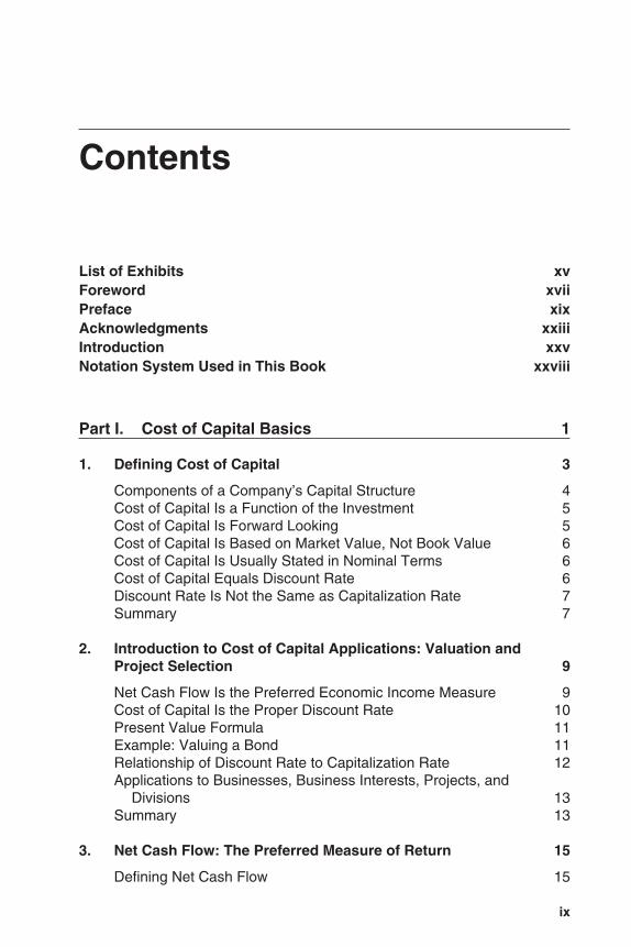
Contents
List of Exhibits xvForeword xviiPreface xixAcknowledgments xxiiiIntroduction xxvNotation System Used in This Book xxviii
Part I. Cost of Capital Basics 1
1. Defining Cost of Capital 3
Components of a Company’s Capital Structure 4Cost of Capital Is a Function of the Investment 5Cost of Capital Is Forward Looking 5Cost of Capital Is Based on Market Value, Not Book Value 6Cost of Capital Is Usually Stated in Nominal Terms 6Cost of Capital Equals Discount Rate 6Discount Rate Is Not the Same as Capitalization Rate 7Summary 7
2. Introduction to Cost of Capital Applications: Valuation andProject Selection 9
Net Cash Flow Is the Preferred Economic Income Measure 9Cost of Capital Is the Proper Discount Rate 10Present Value Formula 11Example: Valuing a Bond 11Relationship of Discount Rate to Capitalization Rate 12Applications to Businesses, Business Interests, Projects, and
Divisions 13Summary 13
3. Net Cash Flow: The Preferred Measure of Return 15
Defining Net Cash Flow 15
Net Cash Flows Should Be Probability-Weighted Expected Values 17
Why Net Cash Flow Is the Preferred Measure of Economic Income 19
Summary 20
4. Discounting versus Capitalizing 21
Capitalization Formula 22Example: Valuing a Preferred Stock 22Functional Relationship between Discount Rate and
Capitalization Rate 23Major Difference between Discounting and Capitalizing 25Gordon Growth Model 25Combining Discounting and Capitalizing (Two-stage Model) 26Equivalency of Discounting and Capitalizing Models 29Midyear Convention 30Converting from After-tax Rate to Pretax Rate 32Summary 32
5. Relationship between Risk and the Cost of Capital 34
Defining Risk 34Types of Risk 35How Risk Impacts the Cost of Capital 36Cost of Equity Capital 37Cost of Conventional Debt and Preferred Equity Capital 37Cost of Overall Invested Capital 37Summary 37
6. Cost Components of a Company’s Capital Structure 39
Debt 40Preferred Equity 41Convertible Debt or Preferred Stock 42Common Stock or Partnership Interests 42Summary 43
7. Weighted Average Cost of Capital 45
When to Use Weighted Average Cost of Capital 45Weighted Average Cost of Capital Formula 46Computing WACC for a Public Company 46Computing WACC for a Private Company 48Should an Actual or a Hypothetical Capital Structure Be Used? 52Summary 52
x Contents
Part II. Estimating the Cost of Equity Capital 55
8. Build-up Models 57
Formula for the Equity Cost of Capital Build-up Model 58Risk-free Rate 58Equity Risk Premium 60Small Stock Premium 64Company-specific Risk Premium 65Example of a Build-up Model 67Summary 68
9. Capital Asset Pricing Model 70
Concept of Systematic Risk 70Background of the Capital Asset Pricing Model 71Systematic and Unsystematic Risk 71Using Beta to Estimate Expected Rate of Return 72Expanding CAPM to Incorporate Size Premium and Specific Risk 75Expanded CAPM Cost of Capital Formula 76Assumptions Underlying the Capital Asset Pricing Model 77Recent Research on the Equity Risk Premium 78Summary 79
10. Proper Use of Betas 80
Estimation of Beta 80Differences in Estimation of Beta 82Levered and Unlevered Betas 83Modified Betas: Shrunk and Lagged 86Summary 87
11. Size Effect 90
Ibbotson Associates Studies 90Standard & Poor’s Corporate Value Consulting Studies
(formerly the PricewaterhouseCoopers Studies) 93Extension of Data to Smaller Size Categories:
Results from the Pratt’s Stats™ Database 99Summary 107
12. DCF Method of Estimating Cost of Capital 109
Theory of the DCF Method 109Mechanics of the DCF Method 110Single-stage DCF Model 110Multistage DCF Models 113Sources of Information 115Summary 115
Contents xi
13. Using Ibbotson Associates Cost of Capital Data 116Michael W. Barad and Tara McDowell
Stocks, Bonds, Bills and Inflation 117Cost of Capital Yearbook 128Ibbotson Beta Book 134Cost of Capital Center 139
14. Arbitrage Pricing Model 143
Explanation of the APT Model 143APM Formula 144Summary 147
Part III. Other Topics Related to Cost of Capital 149
15. Minority versus Control Implications of Cost of Capital Data 151
Minority versus Control Has Little or No Impact on Cost of Capital 153
Company Efficiency versus Shareholder Exploitation 154Impact of the Standard of Value 155Under What Circumstances Should a Control Premium
Be Applied? 155A Tale of Two Markets 156Many Takeovers at Less Than Public Trading Price 157Summary 163
16. Handling the Discount for Lack of Marketability 165
Discrete Percentage Discount for Lack of Marketability 165Building the Discount for Lack of Marketability into the
Discount Rate 173Summary 174
17. How Cost of Capital Relates to the Excess Earnings Method of Valuation 176
Basic “Excess Earnings” Valuation Method 178Cost of Capital Reasonableness Check 180Vagaries of the Excess Earnings Method 182Summary 183
18. Common Errors in Estimation and Use of Cost of Capital 184
Confusing Discount Rates with Capitalization Rates 185Using the Firm’s Cost of Capital to Evaluate a More or Less
Risky Acquisition or Project 185
xii Contents
Mistaking Historical Rates of Return for Expected Rates of Return 185
Mismatching the Discount Rate with the Economic Income Measure 186
Performing an Excess Earnings Method Valuation That Results in an Unrealistic Cost of Capital 188
Projecting Growth beyond That Which the Capital Being Valued Will Support 189
Internally Inconsistent Capital Structure Projection 190Assumptions That Produce a Standard of Value Other Than
That Specified in the Valuation Engagement 190Incorrect or Inadequately Supported Data in Estimating the
Cost of Equity 190Summary 191
19. Cost of Capital in the Courts 193
Cost of Capital in Shareholder Disputes 193Cost of Capital in the Tax Court 194Cost of Capital in Family Law 197Cost of Capital in Bankruptcy Reorganizations 198Cost of Capital Included in Damages 202Cost of Capital in Utility Rate-setting 203Taxicab Lease Rates 204Summary 205
20. Cost of Capital in Ad Valorem Taxation 207Carl R.E. Hoemke
Introduction to Ad Valorem Taxation 208Some Examples of Law That Promulgates the Definition of
Income to Discount 209General Categories of Legislative Constraints Where
Adjustments to the Cost of Capital Are Necessary 209Cost of Capital in a Constant, Perpetual Cash Flow Scenario 210Different Types of Adjustments 210Other Adjustments to the Cost of Capital 221Summary 223
21. Capital Budgeting and Feasibility Studies 224
Invest for Returns above Cost of Capital 224DCF Is Best Corporate Decision Model 225Focus on Net Cash Flow 225Adjusted Present Value Analysis 225Use Target Cost of Capital over Life of Project 227Summary 227
Contents xiii
22. Central Role of Cost of Capital in Economic Value Added 229Joel M. Stern, G. Bennett Stewart III, and Donald H. Chew Jr.
EVA Financial Management System 232EVA and the Corporate Reward System 233Summary 237
Appendixes 239
Appendix A Bibliography 241Appendix B Courses and Conferences 252Appendix C Data Resources 254Appendix D Developing Cost of Capital (Capitalization Rates
and Discount Rates) Using ValuSource PRO Software 264Z. Christopher Mercer, ASA, CFA
Appendix E Iterative Process Using CAPM to Calculate the Cost of Equity Component of the Weighted Average Cost of Capital 274Harold G. Martin, Jr., MBA, CPA/ABV, ASA, CFE
Appendix F International Glossary of Business Valuation 292Terms
Appendix G Converting After-tax Discount Rates to PretaxDiscount Rates 300
CPE Self-study Examination 303
Index 314
xiv Contents
xv
List of Exhibits
3.1 Cash Flow Expectation Tables3.2 Cash Flow Expectation Graphs6.1 Capital Structure Components8.1 Stock Market Return and Equity Risk Premium Over Time8.2 Summary of Development of Equity Discount Rate9.1 Security Market Line9.2 Capital Asset Pricing Model Method of Estimating Equity Discount Rate10.1 Example of One Common Method for Calculation of Beta10.2 Computing Unlevered and Relevered Betas10.3 Excerpt from Second 2001 Edition Beta Book11.1 Long-term Returns in Excess of CAPM Estimation for Decile Portfolios of
the NYSE/AMEX/NASDAQ, with Tenth Decile Split (1926–2000)11.2 Size-Decile Portfolios of the NYSE/AMEX/NASDAQ, Largest Company
and Its Market Capitalization by Decile (September 30, 2000)11.3 Premiums over Long-term Riskless Rate11.4 Premiums over CAPM11.5 Companies Ranked by Measure of Risk11.6 Pratt’s Stats™ Median Values by SIC Code13.1 Build-up versus CAPM Cost of Equity Models13.2 Security Market Line versus Size-Decile Portfolios of the NYSE/AMEX/
NASDAQ (1926–2000)13.3 Long-term Returns in Excess of CAPM Estimation for Decile Portfolios of
the NYSE/AMEX/NASDAQ (1926–2000)13.4 Sample Page from the 2001 Cost of Capital Yearbook13.5 Sample Page from the Beta Book Second 2001 Edition13.6 International Cost of Capital Report13.7 International Cost of Capital Perspectives Report14.1 Explanation of APT Risk Factors14.2 APT and CAPM Cost of Equity Capital Estimates Example15.1 “Levels of Value” in Terms of Characteristics of Ownership15.2 Schematic Relationship of Stock Market and M&A Market15.3 Mergerstat/Shannon Pratt’s Control Premium Study™ Takesovers from
1998 to 200116.1 Summary of Restricted Stock Transaction Studies16.2 FMV Opinions, Inc. Restricted Stock Study Transaction Report
3953 P-00 8/29/02 2:41 PM Page xv

16.3 Summary of Discounts for Private Transaction P/E Multiples Compared toPublic Offering P/E Multiples Adjusted for Changes in Industry P/E Multiples
16.4 Value of Marketability as Illustrated in Initial Public Offerings of CommonStock
16.5 Results of Valuation Advisors Study for 200016.6 Sample Transaction Report from Valuation Advisors Lack of Marketability
Discount Study™16.7 Estimating Cost of Capital, Including Illiquidity Factor17.1 Revenue Ruling 68-60921.1 Pros and Cons of Approaches to Corporate Decision MakingD.1 Calculating Build-up or CAPM Discount and Capitalization RatesD.2 Calculating Indicated Values
xvi List of Exhibits
3953 P-00 8/29/02 2:41 PM Page xvi
xvii
Foreword
Many of us have been anxiously awaiting Shannon Pratt’s second edition of Costof Capital: Estimation and Applications, following the successful first edition. Thecurrent edition includes a totally rewritten and expanded chapter on how to use Ibbot-son Associates’ new Stocks, Bonds, Bills, and Inflation® Valuation Edition Yearbook,emphasizing the easy-to-use build-up method, as well as providing clarifying links tomany of our other methods and products throughout this book. Shannon also hasadded a chapter on the cost of capital in Economic Value Added (EVA)®, includednew sections and data on lack of marketability, control, and minority interests, andprovided results from new studies on micro-stocks, sold companies, and price valua-tion multiples.
Shannon Pratt has been a leader in the valuation field for decades, writing nu-merous books, operating a consulting and valuation firm, and producing such indus-try resources as Shannon Pratt’s Business Valuation Update® and Pratt’s Stats™. Hehas been a collector and provider of data and information on prices, ratios, deals, andsales, as well as legal and tax developments in the industry. He has been a developerand compiler of theoretical approaches and practical procedures. It is particularlyhelpful that he has turned his attention to the cost of capital.
The cost of capital is a critical component of both the valuation and the corpo-rate decision-making processes. Yet the theory is much less understood than the the-ory of forecasting expected cash flows. For example, increasing leverage may increasethe cost of equity and the cost of debt without necessarily affecting the weighted av-erage cost of capital. Cost of capital procedures are a frequent source of major logi-cal errors, not just judgment errors. Mistakes of this type can leave the decisionmaker or appraiser vulnerable, inasmuch as he or she can actually be proven wrong.This is an area where practitioners badly need a guide such as Cost of Capital, so theyunderstand what they are doing.
The cost of capital is one of the key components in valuation. But it is rarely ob-served directly. Instead, it must be estimated. Numerous models can be used to estimatethe cost of capital, such as the build-up models, the Capital Asset Pricing Model, thediscounted cash flow model, and the arbitrage pricing theory. These models may re-quire adjustments for risk, capital structure, size of company, and so forth. There arealso many ways to estimate the parameters in these models. All of them may be com-bined in the weighted average cost of capital. Ibbotson Associates is the provider ofmany of these estimates. I certainly welcome the second edition of Cost of Capital as a
3953 P-00 8/29/02 2:41 PM Page xvii

publication that can help to educate practitioners about what the data mean and howthey can use them.
This book is beginning to serve as the standard reference on cost of capital. It willjoin Shannon Pratt’s set of valuation books in providing the theoretical foundationsand practical procedures in valuation, capital budgeting, and investment decision mak-ing. However, cost of capital is the most challenging subject in valuation, with therichest data and most complex issues. I am personally enthusiastic about adding thisbook to my reference library.
Roger G. IbbotsonChairman, Ibbotson AssociatesProfessor in Practice, Yale School of Management
xviii Foreword
3953 P-00 8/29/02 2:41 PM Page xviii
xix
Preface
Cost of capital estimation is at once the most critical and the most difficult elementof most business valuations and capital expenditure decisions. This book provides aprimer for both the neophyte and the experienced financial analyst in making or as-sessing the cost of capital estimate.
The book is fully indexed and designed to be both a straightforward tutorial anda handy desk reference for:
• Business valuation analysts
• Corporate finance analysts
• CPAs
• Judges and attorneys
• Investment bankers and business sale intermediaries
• Academicians and students
WHAT’S NEW IN THIS EDITION
The second edition is not only updated with current data and references since thefirst edition in 1998, but is also greatly expanded with additional material:
• A new chapter on cost of capital in Economic Value Added (EVA)®.
• A new appendix detailing the iterative process in calculating the cost of equitycomponent in the weighted average cost of capital (WACC).
• A totally new and expanded chapter on using Ibbotson data, with emphasis on thenew Stocks, Bonds, Bills, and Inflation® (SBBI) Valuation Edition Yearbook,which was inaugurated in 1999 and has been updated annually.
• The chapter on the build-up method has been modified to reflect use of additionaldata available in the SBBI Valuation Edition.
• Two new sections have been added to the minority versus control implicationschapter. One is a study conducted on the Mergerstat/Shannon Pratt’s ControlPremium Study™ database showing, among other things, that 16% of takeovers ofpublic companies occur at prices below their public trading prices! The other is a“tale of two markets,” making the point that the merger market is a separate market
3953 P-00 8/29/02 2:41 PM Page xix
from the public stock market. These sections provide support for Roger Ibbotson’scontention that cost of capital is not influenced by control or minority status.
• Additional studies on the small stock phenomenon by Roger Grabowski andDavid King, as well as updates of their original studies.
• In addition to the 25-sector-size total returns for the groups plus the “financiallydistressed” group, they have done a parallel study on premiums over CAPM forthe same size categories.
• They have added a new study on costs of capital related to three risk factors de-rived from company financial statements.
• A new study on the Pratt’s Stats™ sold company database comparing median price/EBITDA multiples and price/sales multiples for transactions from $10 million to$50 million in deal size, with transactions from $1 million to $10 million, andunder $10 million for eight broad industry groups, giving evidence that the size ef-fect does continue below $10 million market value.
• The chapter on handling the discount for lack of marketability has been expandedto include summary results of all major discount for lack of marketability studies.In addition, details of two studies that have been newly developed since the firstedition are presented.
• The common errors chapter has been expanded.
• The chapter on cost of capital in the courts has been more than doubled, reflectingcases since the first edition and some previous landmark cases.
• The bibliography and data resources appendixes have been updated and expanded.
• The index has been completely rewritten and expanded, making it much moreuser-friendly and helpful.
SCOPE AND CONTENT OF THE BOOK
My goal has been to make this book a state-of-the-art treatise on cost of capital es-timation, while still making it understandable to the nonprofessional. To this end, theorganization of the book starts with a layperson’s understanding of the basic conceptsand then moves from simpler applications to some of the more complex applicationsregularly found in the marketplace. The presentation is generously supplemented withtables, graphical diagrams, and examples.
This book addresses the following applications:
• Valuation
Businesses and business interests
Intangible assets, including intellectual properties
Other income-generating assets
Ad valorem (property) taxation
xx Preface
3953 P-00 8/29/02 2:41 PM Page xx
• Capital budgeting, feasibility studies, and corporate finance decisions
Capital budgeting and allocation
Feasibility studies
It lays out basic tools that anyone can use immediately either in estimating thecost of capital or in reviewing someone else’s cost of capital estimate:
• Basic cost of capital theory
• How cost of capital is used in business and in business asset valuation and capitalexpenditure decision making:
In the income approach
In the market approach
In the excess earnings method
• The basic mathematical formulas used, with clear explanations
• Comprehensive sources of information
• Clear and complete definitions of commonly used terminology
• Common errors—how to identify them in other people’s work products and howto avoid them
• A comprehensive bibliography
CPE CREDIT
A self-study mail-in quiz at the back of the book will entitle the reader to eighthours of CPE credit.
COST OF CAPITAL WORKBOOK
We have also prepared a Cost of Capital Workbook in conjunction with this sec-ond edition. Section One of the workbook has questions and computational problemsbased on each chapter in this text, and Section Two has answers to the questions andsolutions to the problems. This will provide hands-on experience for those who de-sire to practice or test their understanding of the concepts in this book. It will also bevaluable preparation for those taking examinations in the AIMR, ASA, AICPA, IBA,NACVA, or CICBV programs. The workbook also contains a mail-in quiz for eighthours of CPE credit as well.
COST OF CAPITAL IS DYNAMIC
Cost of capital is dynamic, in terms of both current market statistics and theo-retical development. There has been an acceleration of research and literature on cost
Preface xxi
3953 P-00 8/29/02 2:41 PM Page xxi

of capital in recent years. While this book draws heavily on Ibbotson Associatesdata, many are challenging its applications today, including both the general equityrisk premium and data on the size effect. There is growing emphasis on what in thisbook we call the “DCF method” of estimating the cost of equity capital (Chapter 12).As noted in that chapter, the DCF method consistently produces lower estimates ofthe cost of equity capital than either the build-up model or the Capital Asset PricingModel (CAPM). A few references to recent views are presented at the end of Chap-ter 9 on CAPM, and others are scattered throughout the Bibliography.
Readers can keep up-to-date on both market and theoretical developmentthrough the monthly “Cost of Capital Update” and “Market Data Corner” sections inShannon Pratt’s Business Valuation Update®. Please contact us with any commentsor questions on the book, and/or for a complimentary current issue of the newsletter,at the following address or at (888) BUS-VALU [(888) 287-8258], fax (503) 291-7955, (800) 846-2291.
Shannon P. Pratt7412 S.W. Beaverton-Hillsdale HighwaySuite 106Portland, OR 97225e-mail: [email protected]
xxii Preface
3953 P-00 8/29/02 2:41 PM Page xxii
xxiii
Acknowledgments
This book has benefited immensely from review by many people with a highlevel of knowledge and experience in cost of capital and valuation. The followingpeople reviewed the manuscript, and the book reflects their invaluable efforts and le-gions of constructive suggestions:
Michael W. BaradIbbotson AssociatesChicago, Ill.
Stephen J. BravoApogee Business ValuationsFramingham, Mass.
Roger GrabowskiStandard & Poor’sCorporate Value ConsultingChicago, Ill.
James R. HitchnerPhillips Hitchner Group, Inc.Atlanta, Ga.
Harold G. MartinKeiter, Stephens, Hurst, Gary &
ShreavesGlen Allen, Va.
Michael J. MattsonThe Financial Valuation GroupChicago, Ill.
Chad PhillipsBusiness Valuation Resources, LLCPortland, Ore.
James S. RigbyThe Financial Valuation GroupLos Angeles, Calif.
Robert P. SchweihsWillamette Management AssociatesChicago, Ill.
Ronald L. SeigneurSeigneur & Company, P.C., CPAsLakewood, Colo.
Doug TwitchellBusiness Valuation Resources, LLCPortland, Ore.
In addition, I thank Rich Schmitt and William Roper of The Alcar Group andEdwin Burmeister of BIRR Portfolio Analysis, Inc. for review and feedback onChapter 14, “Arbitrage Pricing Model.”
I especially thank Michael W. Barad and Tara McDowell, both of Ibbotson Asso-ciates, for contributing the revised and updated Chapter 13 on using Ibbotson Associ-ates cost of capital data. And I thank Carl R. E. Hoemke of Ernst & Young forcontributing Chapter 20 on using cost of capital in ad valorem (property tax) valuations.I also thank Z. Christopher Mercer of Mercer Capital for Appendix D on using cost ofcapital in conjunction with Wiley ValuSource PRO Software, and Harold G. Martin, ofKeiter, Stephens, Hurst, Gary & Shreaves, P.C., for contributing Appendix E on the it-
3953 P-00 8/29/02 2:41 PM Page xxiii
erative model for estimating cost of equity capital in the weighted average cost of cap-ital. Thanks also to Joel M. Stern, G. Bennett Stewart III, and Donald H. Chew Jr., ofStern Stewart & Co., for permitting the adaptation of an excerpt from their article onEconomic Value Added as Chapter 22.
Janet Marcley of Business Valuation Resources, LLC, provided much assistancein obtaining permissions to reprint material from other sources. For these permis-sions, I thank:
The Alcar Group, Inc.American Society of AppraisersBIRR Portfolio Analysis, Inc.Thomas CopelandEmory Business Valuation, LLCFMV Opinions, Inc.Ibbotson AssociatesMark Lee of Sutter Securities IncorporatedMcGraw-Hill CompaniesPeabody Publishing, LPPractitioners Publishing CompanyStandard & Poors Corporate Value ConsultingStern Stewart & Co.Valuation Advisors, Inc.Willamette Management Associates
Several other individuals at Business Valuation Resources, LLC, contributedsignificantly to this second edition of the book. For their valuable data research con-tributions, I would like to thank Jill Johnson, research analyst, Doug Twitchell, amanager of BVMarketData.comsm, and Alina Niculita, managing editor of ShannonPratt’s Business Valuation Update®. I would also like to thank Chad Phillips, a man-ager of BVMarketData.comsm, and Doug Twitchell for their meticulous review of theformulas and calculations in the first edition. Linda Kruschke, publications depart-ment manager, made considerable improvements to the bibliography and index, andLaurie Morrisey assisted with typing. The bibliography and data resources appendixeswere both greatly enhanced by reference to the 2002 Business Valuation Data, Pub-lications & Internet Directory, which is published annually by Business ValuationResources, LLC, and made possible by the exhaustive efforts of research analysts JillJohnson and Paul Heidt, production manager Michael Thomas, and Alina Niculita.
I greatly appreciate the continuing cooperation of the professionals at JohnWiley & Sons, Inc.: John DeRemigis, executive editor; Judy Howarth, associate ed-itor; and Louise Jacob, associate managing editor.
Last, but not least, the entire project was coordinated by the assiduous efforts ofTanya Hanson, associate editor at Business Valuation Resources, LLC, and projectmanager for this second edition.
Shannon PrattPortland, Oregon
xxiv Acknowledgments
3953 P-00 8/29/02 2:41 PM Page xxiv
xxv
Introduction
PURPOSE AND OBJECTIVE OF THIS BOOK
The purpose of this book is to present both the theoretical development of cost ofcapital estimation and its practical application to valuation, capital budgeting, andrate-setting problems encountered in current practice. It is intended both as a learningtext for those who want to study the subject and as a handy reference for those who areinterested in background or seek direction in some specific aspect of cost of capital.
The objective is to serve two primary categories of users:
1. The practitioner who seeks a greater understanding of the latest theory and prac-tice in cost of capital estimation
2. The reviewer who needs to make an informed evaluation of someone else’smethodology and data used to produce a cost of capital estimate
OVERVIEW
The reader can expect the following:
• The theory of what drives the cost of capital
• The models currently in use to estimate cost of capital
• The data available as inputs to the models to estimate cost of capital
• How to use the cost of capital estimate in:
Valuation
Feasibility studies
Corporate finance decisions
• How to reflect minority/control and marketability considerations
• Terminology, with its unfortunately varied and sometimes ambiguous usage incurrent-day financial analysis
IMPORTANCE OF THE COST OF CAPITAL
The cost of capital estimate is the essential link that enables us to convert astream of expected income into an estimate of present value. Doing this allows us to
3953 P-00 8/29/02 2:41 PM Page xxv
make informed pricing decisions for purchases and sales and a comparison of one in-vestment opportunity against another.
COST OF CAPITAL ESSENTIAL IN THE MARKET
In valuation and financial decision making, the cost of capital estimate is just asimportant as the estimate of the expected amounts of income to be discounted or cap-italized. Yet we continually see income estimates laboriously developed and then con-verted to estimated value by a cost of capital that is practically pulled out of thin air.
In the marketplace, better-informed cost of capital estimation will improve liter-ally billions of dollars’ worth of financial decisions every day.
SOUND SUPPORT ESSENTIAL IN THE COURTROOM
In the courts, billions of dollars turn on experts’ disputed cost of capital estimatesin many contexts:
• Gift, estate, and income tax disputes
• Dissenting stockholder suits
• Corporate and partnership dissolutions
• Marital property settlements
• Employee stock ownership plans (ESOPs)
• Ad valorem (property) taxes
• Utility rate-setting
• Damages calculations
Fortunately, courts are becoming unwilling to accept “Trust me, I’m a great ex-pert” in these disputes and instead are carefully weighing the quality of supportingevidence presented by opposing sides. Because cost of capital is critical to the valu-ation of any ongoing business, the thorough understanding, analysis, and presentationof cost of capital issues will go a long way toward carrying the day in a battle of ex-perts in a legal setting.
ORGANIZATION OF THIS BOOK
Part I. Cost of Capital Basics
The first chapter defines cost of capital. The second chapter describes, in a gen-eral sense, how it is used in business valuation and capital budgeting. Chapter 3 de-fines net cash flow and explains why it is the preferred economic income variable forvaluation and capital budgeting. Chapter 4 explains the difference between discount-
xxvi Introduction
3953 P-00 8/29/02 2:41 PM Page xxvi
ing and capitalizing. Chapter 5 addresses the concept of risk and the impact of risk onthe cost of capital. From there we move to the various components of a company’scapital structure and the concept of a weighted average of the cost of each component(weighted average cost of capital).
Part II. Estimating the Cost of Equity Capital
The second part explores cost of capital estimation. This includes the build-upmodel, the Capital Asset Pricing Model (CAPM), discounted cash flow (DCF) mod-els, and arbitrage pricing theory (APT) for estimating the cost of equity.
Part III. Other Topics Related to Cost of Capital
The third part addresses commonly encountered variations in cost of capital ap-plication:
• Minority versus controlling interest valuations
• Handling discounts for lack of marketability
• Court case examples of cost of capital issues
• How cost of capital relates to the excess earnings valuation method
• Ad valorem applications
• Cost of capital in Economic Value Added (EVA®)
• Common errors
Appendixes
The appendixes provide sources for follow-up to this book, including a detailedbibliography, cost of capital courses and conferences, sources for the current dataneeded to implement cost of capital estimation, a ValuSource PRO software section,and a detailed explanation of the iterative process for cost of equity capital estimationin the context of the weighted average cost of capital (WACC).
SUMMARY
The book is designed to serve as both a primer and a reference source.Part I covers cost of capital basics. Part II covers the methods generally used to
estimate cost of equity capital. Part III covers a variety of topics commonly encoun-tered in cost of capital applications. The appendixes provide a directory for furtherstudy, data sources, a discussion of using ValuSource PRO software, and a detailedexplanation and illustration of the iterative process to estimating cost of equity in theWACC.
Introduction xxvii
3953 P-00 8/29/02 2:41 PM Page xxvii
xxviii
Notation System Used inThis Book
A source of confusion for those trying to understand financial theory and meth-ods is that financial writers have not adopted a standard system of notation. The fol-lowing notation system is adapted from the fourth edition of Valuing a Business: TheAnalysis and Appraisal of Closely Held Companies, by Shannon P. Pratt, Robert F.Reilly, and Robert P. Schweihs (New York: McGraw-Hill, 2000).
VALUE AT A POINT IN TIME
PV = Present valueFV = Future valueMVIC = Market value of invested capital
COST OF CAPITAL AND RATE OF RETURN VARIABLES
k = Discount rate (generalized)ke = Discount rate for common equity capital (cost of common equity
capital). Unless otherwise stated, it generally is assumed that thisdiscount rate is applicable to net cash flow available to commonequity.
ke(pt) = Cost of equity prior to tax effectkp = Discount rate for preferred equity capitalkd = Discount rate for debt (net of tax effect, if any)
(Note: For complex capital structures, there could be more thanone class of capital in any of the preceding categories, requiringexpanded subscripts.)
kd(pt) = Cost of debt prior to tax effectkni = Discount rate for equity capital when net income rather than net
cash flow is the measure of economic income being discountedc = Capitalization ratece = Capitalization rate for common equity capital. Unless otherwise
stated, it generally is assumed that this capitalization rate isapplicable to net cash flow available to common equity.
cni = Capitalization rate for net incomecp = Capitalization rate for preferred equity capital
3953 P-00 8/29/02 2:41 PM Page xxviii
Notation System Used in This Book xxix
cd = Capitalization rate for debt(Note: For complex capital structures, there could be more thanone class of capital in any of the preceding categories, requiringexpanded subscripts.)
t = Tax rate (expressed as a percentage of pretax income)R = Rate of returnRf = Rate of return on a risk-free securityE(R) = Expected rate of returnE(Rm) = Expected rate of return on the “market” (usually used in the
context of a market for equity securities, such as the New YorkStock Exchange [NYSE] or Standard & Poor’s [S&P] 500)
E(Ri) = Expected rate of return on security iB = Beta (a coefficient, usually used to modify a rate of return
variable)BL = Levered betaBU = Unlevered betaRP = Risk premiumRPm = Risk premium for the “market” (usually used in the context of a
market for equity securities, such as the NYSE or S&P 500)RPs = Risk premium for “small” stocks (usually average size of lowest
quintile or decile of NYSE as measured by market value ofcommon equity) over and above RPm
RPu = Risk premium for unsystematic risk attributable to the specificcompany
RPi = Risk premium for the ith securityK1 … Kn = Risk premium associated with risk factor 1 through n for the
average asset in the market (used in conjunction with arbitragepricing theory)
WACC = Weighted averaged cost of capital
INCOME VARIABLES
E = Expected economic income (in a generalized sense; i.e., could bedividends, any of several possible definitions of cash flows, netincome, etc.)
NI = Net income (after entity-level taxes)NCFe = Net cash flow to equityNCFf = Net cash flow to the firm (to overall invested capital, or entire
capital structure, including all equity and long-term debt)PMT = Payment (interest and principal payment on debt security)D = DividendsT = Tax (in dollars)GCF = Gross cash flow (usually net income plus noncash charges)EBT = Earnings before taxes
3953 P-00 8/29/02 2:41 PM Page xxix
EBIT = Earnings before interest and taxesEBDIT = Earnings before depreciation, interest, and taxes (“Depreciation”
in this context usually includes amortization. Some writers useEBITDA to specifically indicate that amortization is included.)
EBITDA = Earnings before interest, taxes, depreciation, and amortization
PERIODS OR VARIABLES IN A SERIES
i = The ith period or the ith variable in a series (may be extended tothe jth variable, the kth variable, etc.)
n = The number of periods or variables in a series, or the last numberin a series
∞ = Infinity0 = Period0, the base period, usually the latest year immediately
preceding the valuation date
WEIGHTINGS
W = WeightWe = Weight of common equity in capital structureWp = Weight of preferred equity in capital structureWd = Weight of debt in capital structure
(Note: For purposes of computing a weighted average cost ofcapital [WACC], it is assumed that preceding weightings are atmarket value.)
GROWTH
g = Rate of growth in a variable (e.g., net cash flow)
MATHEMATICAL FUNCTIONS
∑ = Sum of (add all the variables that follow)∏ = Product of (multiply together all the variables that follow)x̄ = Mean average (the sum of the values of the variables divided by
the number of variables)G = Geometric mean (the product of the values of the variables taken
to the root of the number of variables)
xxx Notation System Used in This Book
3953 P-00 8/29/02 2:41 PM Page xxx
PART I
Cost of Capital Basics
3953 P-01 8/29/02 2:18 PM Page 1

3953 P-01 8/29/02 2:18 PM Page 2
3
Chapter 1
Defining Cost of CapitalComponents of a Company’s Capital StructureCost of Capital Is a Function of the InvestmentCost of Capital Is Forward LookingCost of Capital Is Based on Market Value, Not Book ValueCost of Capital Is Usually Stated in Nominal TermsCost of Capital Equals Discount RateDiscount Rate Is Not the Same as Capitalization RateSummary
Cost of capital is the expected rate of return that the market requires in order toattract funds to a particular investment. In economic terms, the cost of capital for aparticular investment is an opportunity cost—the cost of forgoing the next best alter-native investment. In this sense, it relates to the economic principle of substitution—that is, an investor will not invest in a particular asset if there is a more attractivesubstitute.
The “market” refers to the universe of investors who are reasonable candidates toprovide funds for a particular investment. Capital or funds are usually provided in theform of cash, although in some instances capital may be provided in the form of otherassets. The cost of capital usually is expressed in percentage terms, that is, the annualamount of dollars that the investor requires or expects to realize, expressed as a per-centage of the dollar amount invested.
Put another way:
Since the cost of anything can be defined as the price one must pay to get it, the cost ofcapital is the return a company must promise in order to get capital from the market, eitherdebt or equity. A company does not set its own cost of capital; it must go into the mar-ket to discover it. Yet meeting this cost is the financial market’s one basic yardstick fordetermining whether a company’s performance is adequate.1
As the preceding quote suggests, most of the information for estimating the cost ofcapital for any company, security, or project comes from the investment markets. Thecost of capital is always an expected return. Thus, analysts and would-be investorsnever actually observe it. We analyze many types of market data to estimate the costof capital for a company, security, or project in which we are interested.
As Roger Ibbotson put it, “The Opportunity Cost of Capital is equal to the returnthat could have been earned on alternative investments at a specific level of risk.”2 In
3953 P-01 8/29/02 2:18 PM Page 3
other words, it is the competitive return available in the market on a comparable in-vestment, risk being the most important component of comparability.
COMPONENTS OF A COMPANY’S CAPITAL STRUCTURE
The term “capital” in this context means the components of an entity’s capitalstructure. The primary components of a capital structure include:
• Long-term debt
• Preferred equity (stock or partnership interests with preference features, such asseniority in receipt of dividends or liquidation proceeds)
• Common equity (stock or partnership interests at the lowest or residual level of thecapital structure)
There may be more than one subcategory in any or all of the above categories ofcapital. Also, there may be related forms of capital, such as warrants or options. Eachcomponent of an entity’s capital structure has its unique cost, depending primarily onits respective risk.
Simply and cogently stated, “The cost of equity is the rate of return investors re-quire on an equity investment in a firm.”3
Recognizing that the cost of capital applies to both debt and equity investments,a well-known text states, “Both creditors and shareholders expect to be compensatedfor the opportunity cost of investing their funds in one particular business instead ofothers with equivalent risk.”4
The next quote explains how the cost of capital can be viewed from three differ-ent perspectives:
The cost of capital (sometimes called the expected or required rate of return or the dis-count rate) can be viewed from three different perspectives. On the asset side of a firm’sbalance sheet, it is the rate that should be used to discount to a present value the futureexpected cash flows. On the liability side, it is the economic cost to the firm of attractingand retaining capital in a competitive environment, in which investors (capital providers)carefully analyze and compare all return-generating opportunities. On the investor’sside, it is the return one expects and requires from an investment in a firm’s debt or eq-uity. While each of these perspectives might view the cost of capital differently, they areall dealing with the same number.5
When we talk about the cost of ownership capital (i.e., the expected return to astock or partnership investor), we usually use the phrase “cost of equity capital.” Whenwe talk about the cost of capital to the firm overall (i.e., the average cost of capital forboth ownership interests and debt), we usually use the phrase “weighted average costof capital” (WACC) or “blended cost of capital.”
4 Cost of Capital Basics
3953 P-01 8/29/02 2:18 PM Page 4
COST OF CAPITAL IS A FUNCTION OF THE INVESTMENT
As Ibbotson puts it, “The cost of capital is a function of the investment, not theinvestor.”6 The cost of capital comes from the marketplace. The marketplace is theuniverse of investors for a particular asset.
Brealey and Myers state the same concept: “The true cost of capital depends onthe use to which the capital is put.”7 They make the point that it would be an error toevaluate a potential investment on the basis of a company’s overall cost of capital ifthat investment were more or less risky than the company’s existing business. “Eachproject should be evaluated at its own opportunity cost of capital.”8
When a company uses the cost of capital to evaluate a commitment of capital toan investment or project, it often refers to that cost of capital as the “hurdle rate.” The“hurdle rate” means the minimum expected rate of return that the company would bewilling to accept to justify making the investment. As noted in the previous para-graph, the “hurdle rate” for any given prospective investment may be at, above, orbelow the company’s overall cost of capital, depending on the degree of risk of theprospective investment compared to the company’s overall risk.
The most popular theme of contemporary corporate finance is that companiesshould be making investments, either capital investments or acquisitions, from whichthe returns will exceed the cost of capital for that investment. Doing so creates eco-nomic value added, economic profit, or shareholder value added.9
COST OF CAPITAL IS FORWARD LOOKING
The cost of capital represents investors’ expectations. There are three elementsto these expectations:
1. The “real” rate of return—the amount investors expect to obtain in exchange forletting someone else use their money on a riskless basis
2. Expected inflation—the expected depreciation in purchasing power while themoney is tied up
3. Risk—the uncertainty as to when and how much cash flow or other economic in-come will be received
It is the combination of the first two items above that is sometimes referred to as the“time value of money.” While these expectations may be different for different in-vestors, the market tends to form a consensus with respect to a particular investmentor category of investments. That consensus determines the cost of capital for invest-ments of varying levels of risk.
The cost of capital, derived from investors’ expectations and the market’s con-sensus of those expectations, is applied to expected economic income, usually measuredin terms of cash flows, in order to estimate present values or to compare investment
Defining Cost of Capital 5
3953 P-01 8/29/02 2:18 PM Page 5
alternatives of similar or differing levels of risk. “Present value,” in this context, refersto the dollar amount that a rational and well-informed investor would be willing topay today for the stream of expected economic income being evaluated. In mathemat-ical terms, the cost of capital is the percentage rate of return that equates the stream ofexpected income with its present cash value.
COST OF CAPITAL IS BASED ON MARKET VALUE, NOT BOOK VALUE
The cost of capital is the expected rate of return on some base value. That basevalue is measured as the market value of an asset, not its book value. For example,the yield to maturity shown in the bond quotations in the financial press is based onthe closing market price of a bond, not on its face value. Similarly, the implied costof equity for a company’s stock must be (or should be) based on the market price pershare at which its trades, not on the company’s book value per share of stock. It wasnoted earlier that the cost of capital is estimated from market data. This data refers toexpected returns relative to market prices. By applying the cost of capital derivedfrom market expectations to the expected cash flows (or other measure of economicincome) from the investment or project under consideration, the market value can beestimated.
COST OF CAPITAL IS USUALLY STATED IN NOMINAL TERMS
Keep in mind that we have talked about expectations, including inflation. The returnan investor requires includes compensation for reduced purchasing power of the dol-lar over the life of the investment. Therefore, when the analyst or investor applies thecost of capital to expected returns to estimate value, he or she must also include ex-pected inflation in those expected returns.
This obviously assumes that investors have reasonable consensus expectationsregarding inflation. For countries subject to unpredictable hyperinflation, it is some-times more practical to estimate cost of capital in real terms rather than in nominalterms.
COST OF CAPITAL EQUALS DISCOUNT RATE
The essence of the cost of capital is that it is the percentage return that equatesexpected economic income with present value. The expected rate of return in thiscontext is called a discount rate. By a “discount rate,” the financial community meansan annually compounded rate at which each increment of expected economic incomeis discounted back to its present value. A discount rate reflects both time value ofmoney and risk and therefore represents the cost of capital. The sum of the discountedpresent values of each future period’s incremental cash flow or other measure of return
6 Cost of Capital Basics
3953 P-01 8/29/02 2:18 PM Page 6
equals the present value of the investment, reflecting the expected amounts of returnover the life of the investment. The terms “discount rate,” “cost of capital,” and “re-quired rate of return” are often used interchangeably.
The economic income referenced here represents total expected returns. In otherwords, this economic income includes increments of cash flow realized by the investorwhile holding the investment, as well as proceeds to the investor on liquidation of theinvestment. The rate at which these expected future total returns are reduced to pre-sent value is the discount rate, which is the cost of capital (required rate of return) fora particular investment.
DISCOUNT RATE IS NOT THE SAME AS CAPITALIZATION RATE
Discount rate and capitalization rate are two distinctly different concepts. As notedin the previous section, discount rate equates to cost of capital. It is a rate applied toall expected incremental returns to convert the expected return stream to a presentvalue.
A capitalization rate, however, is merely a divisor applied to one single elementof return to estimate a present value. The only instance in which the discount rate isequal to the capitalization rate is when each future increment of expected return isequal (i.e., no growth), and the expected returns are in perpetuity. One of the few ex-amples would be a preferred stock paying a fixed amount of dividend per share inperpetuity.
In the unique case where an amount of return is expected to grow at a constantrate in perpetuity, the capitalization rate applicable to that expected return is equal tothe discount rate less the expected rate of growth. The relationship between discountand capitalization rates is discussed further in future chapters, especially in Chapter4 on “Discounting versus Capitalizing.”
SUMMARY
As stated in the Introduction, “The cost of capital estimate is the essential link thatenables us to convert a stream of expected income into an estimate of present value.”
Cost of capital has several key characteristics:
• It is market driven. It is the expected rate of return that the market requires to com-mit capital to an investment.
• It is a function of the investment, not the investor.
• It is forward looking, based on expected returns.
• The base against which cost of capital is measured is market value, not bookvalue.
• It is usually measured in nominal terms, that is, including expected inflation.
Defining Cost of Capital 7
3953 P-01 8/29/02 2:18 PM Page 7
• It is the link, called a discount rate, that equates expected future returns for the lifeof the investment with the present value of the investment at a given date.
Notes
1. Mike Kaufman, “Profitability and the Cost of Capital,” Chapter 8 in Handbook of Bud-geting, 4th ed., Robert Rachlin, ed. (New York: John Wiley & Sons, Inc., 1999), 8-3.
2. Ibbotson Associates, Cost of Capital Workshop (Chicago: Ibbotson Associates, 1999),Chapter 1, p. 2.
3. Aswath Damodaran, Investment Valuation: Tools and Techniques for Determining theValue of Any Asset, 2d ed. (New York: John Wiley & Sons, Inc., 2000), 182.
4. Tom Copeland, Tim Koller, and Jack Murrin, Valuation: Measuring and Managing theValue of Companies, 3d ed. (New York: John Wiley & Sons, Inc., 2000), 201.
5. Stocks, Bonds, Bills and Inflation, Valuation Edition 2002 Yearbook (Chicago: IbbotsonAssociates, 2002), 23.
6. Ibbotson Associates, Cost of Capital Workshop (Chicago: Ibbotson Associates, 1999),Chapter 1, p. 7.
7. Richard A. Brealey and Stewart C. Myers, Principles of Corporate Finance, 6th ed.(Boston: Irwin McGraw-Hill, 2000), 222.
8. Ibid. at 221.9. See, for example, Copeland et al., Valuation; also see Alfred Rappaport, Creating Share-
holder Value, rev. ed. (New York: The Free Press, 1998).
8 Cost of Capital Basics
3953 P-01 8/29/02 2:18 PM Page 8
9
Chapter 2
Introduction to Cost of Capital Applications:Valuation and ProjectSelectionNet Cash Flow Is the Preferred Economic Income MeasureCost of Capital Is the Proper Discount RatePresent Value FormulaExample: Valuing a BondRelationship of Discount Rate to Capitalization RateApplications to Businesses, Business Interests, Projects, and DivisionsSummary
Cost of capital has many applications, the two most common being valuation andcapital investment project selection. These two applications are very closely related.This chapter discusses these two applications in very general terms so the reader canquickly understand how the cost of capital is used every day in valuations and financialdecisions worth billions of dollars. Later chapters discuss these applications in moredetail.
NET CASH FLOW IS THE PREFERRED ECONOMIC INCOME MEASURE
For the purpose of this chapter, we will assume that the measure of economicincome to which cost of capital will be applied is net cash flow (sometimes calledfree cash flow). Net cash flow is discretionary cash available to be paid out to capitalstakeholders (e.g., dividends, withdrawals, discretionary bonuses) without jeopardizingthe projected ongoing operations of the business. We will provide a more exact def-inition of net cash flow in Chapter 3.
Net cash flow is the measure of economic income on which most financial analyststoday prefer to focus for both valuation and capital investment project selection. Weexplain the reasons for this preference in more detail in Chapter 3. Net cash flow rep-resents money available to stakeholders. Most analysts prefer this measure of income
3953 P-02 8/29/02 2:18 PM Page 9
because it obviates owners’ discretionary disposal of company funds. Although thecontemporary literature of corporate finance widely embraces a preference for net cashflow as the relevant economic income variable to which to apply cost of capital forvaluation and decision making, there is still a contingent of analysts who like to focuson accounting income.1
COST OF CAPITAL IS THE PROPER DISCOUNT RATE
At the end of Chapter 1, it was said that the cost of capital is customarily used asa discount rate to convert expected future returns to a present value. This concept issummarized succinctly by Brealey and Myers: “Value today always equals future cashflow discounted at the opportunity cost of capital.”2
In this context, let us keep in mind critical characteristics of a discount rate:
• Definition: A discount rate is a yield rate used to convert anticipated future pay-ments or receipts into present value (i.e., a cash value as of today or as of a specifiedvaluation date).
• The discount rate represents the total rate of return that the investor expects to re-alize on the amount invested.
The use of the cost of capital to estimate present value thus requires two sets ofestimates:
1. The numerator: The expected amount of return on the investment in each futureperiod over the life of the investment
2. The denominator: The discount rate, which is the cost of capital
Usually analysts and investors make the simplifying assumption that the cost ofcapital is constant over the life of the investment and use the same cost of capital toapply to each increment of expected future return. There are, however, special casesin which analysts might choose to estimate a discrete cost of capital to apply to theexpected return in each future period. (An example is when the analyst anticipates achanging weighted average cost of capital because of a changing capital structure.)The above notwithstanding, well-known author, professor, and consultant Dr. AlfredRappaport espouses a constant cost of capital in his 1998 edition of Creating Share-holder Value:
The appropriate rate for discounting the company’s cash flow stream is the weighted av-erage of the costs of debt and equity capital. . . . It is important to emphasize that the rel-ative weights attached to debt and equity, respectively, are neither predicated on dollarsthe firm has raised in the past, nor do they constitute the relative proportions of dollars thefirm plans to raise in the current year. Instead, the relevant weights should be based on theproportions of debt and equity that the firm targets for its capital structure over the long-term planning period.3
The latter view is most widely accepted.
10 Cost of Capital Basics
3953 P-02 8/29/02 2:18 PM Page 10
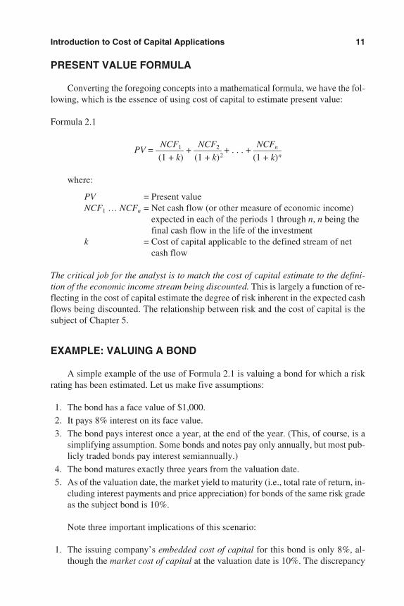
PRESENT VALUE FORMULA
Converting the foregoing concepts into a mathematical formula, we have the fol-lowing, which is the essence of using cost of capital to estimate present value:
Formula 2.1
NCF1 NCF2 NCFnPV = —–—– + ——–– + . . . + –——–(1 + k) (1 + k)2 (1 + k)n
where:
PV = Present valueNCF1 … NCFn = Net cash flow (or other measure of economic income)
expected in each of the periods 1 through n, n being thefinal cash flow in the life of the investment
k = Cost of capital applicable to the defined stream of netcash flow
The critical job for the analyst is to match the cost of capital estimate to the defini-tion of the economic income stream being discounted. This is largely a function of re-flecting in the cost of capital estimate the degree of risk inherent in the expected cashflows being discounted. The relationship between risk and the cost of capital is thesubject of Chapter 5.
EXAMPLE: VALUING A BOND
A simple example of the use of Formula 2.1 is valuing a bond for which a riskrating has been estimated. Let us make five assumptions:
1. The bond has a face value of $1,000.
2. It pays 8% interest on its face value.
3. The bond pays interest once a year, at the end of the year. (This, of course, is asimplifying assumption. Some bonds and notes pay only annually, but most pub-licly traded bonds pay interest semiannually.)
4. The bond matures exactly three years from the valuation date.
5. As of the valuation date, the market yield to maturity (i.e., total rate of return, in-cluding interest payments and price appreciation) for bonds of the same risk gradeas the subject bond is 10%.
Note three important implications of this scenario:
1. The issuing company’s embedded cost of capital for this bond is only 8%, al-though the market cost of capital at the valuation date is 10%. The discrepancy
Introduction to Cost of Capital Applications 11
3953 P-02 8/29/02 2:18 PM Page 11
may be because the general level of interest rates was lower at the time of issuanceof this particular bond, or because the market’s rating of the risk associated withthis bond increased between the date of issuance and the valuation date.
2. If the issuing company wanted to issue new debt on comparable terms as of thevaluation date, it presumably would have to offer investors a 10% yield, the cur-rent market-driven cost of capital for bonds of that risk grade, to induce investorsto purchase the bonds.
3. For purposes of valuation and capital budgeting decisions, when we refer to costof capital, we mean market cost of capital, not embedded cost of capital. (Em-bedded cost of capital is sometimes used in utility rate-making, but this chapterfocuses only on valuation and capital budgeting applications of cost of capital.)
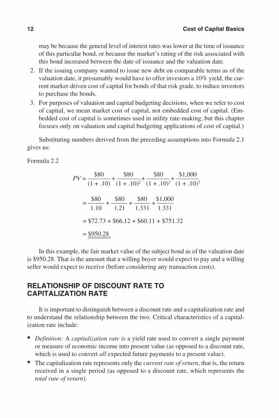
Substituting numbers derived from the preceding assumptions into Formula 2.1gives us:
Formula 2.2
$80 $80 $80 $1,000PV = ———– + ——–— + ——–— + —–——
(1 + .10) (1 + .10)2 (1 + .10)3 (1 + .10)3
$80 $80 $80 $1,000= —–— + —–— + —–— + ——–
1.10 1.21 1.331 1.331
= $72.73 + $66.12 + $60.11 + $751.32
= $950.28= ———–= ———–
In this example, the fair market value of the subject bond as of the valuation dateis $950.28. That is the amount that a willing buyer would expect to pay and a willingseller would expect to receive (before considering any transaction costs).
RELATIONSHIP OF DISCOUNT RATE TO CAPITALIZATION RATE
It is important to distinguish between a discount rate and a capitalization rate andto understand the relationship between the two. Critical characteristics of a capital-ization rate include:
• Definition: A capitalization rate is a yield rate used to convert a single paymentor measure of economic income into present value (as opposed to a discount rate,which is used to convert all expected future payments to a present value).
• The capitalization rate represents only the current rate of return, that is, the returnreceived in a single period (as opposed to a discount rate, which represents thetotal rate of return).
12 Cost of Capital Basics
3953 P-02 8/29/02 2:18 PM Page 12
APPLICATIONS TO BUSINESSES, BUSINESS INTERESTS,PROJECTS, AND DIVISIONS
The same construct can be used to value an equity interest in a company or acompany’s entire invested capital. One projects the cash flows available to the interestto be valued and discounts those cash flows at a cost of capital discount rate that re-flects the risk associated with achieving the particular cash flows. Details of this pro-cedure for valuing entire companies or interests in companies are presented in laterchapters.
Similarly, the same construct can be applied to evaluating a capital budgeting de-cision, such as building a plant or buying equipment. In that case, the cash flows tobe discounted are incremental cash flows, that is, cash flows resulting from the deci-sion that would not occur absent the decision. The early portions of the cash flowstream may be negative while funds are being invested in the project.
The primary relationship to remember is that cost of capital is a function of theinvestment, not of the investor. Therefore, the analyst must evaluate the risk of eachproject under consideration. If the risk of the project is greater or less than the com-pany’s overall risk, then the cost of capital by which that project is evaluated shouldbe commensurately higher or lower than the company’s overall cost of capital.
Although some companies apply a single “hurdle rate” to all proposed projectsor investments, the consensus in the literature of corporate finance is that the rate bywhich to evaluate any investment should be based on the risk of that investment, noton the company’s overall risk that drives the company’s cost of capital. I agree with thisconsensus. If the company invests in something riskier than its normal operations, thecompany’s risk will increase marginally. When this increased risk is recognized andreflected in the market, it will raise the company’s cost of capital. If the returns on theriskier new investment are not great enough to achieve higher returns commensuratewith this higher cost of capital, the result will be a decrease in the stock price and aloss of shareholder value.
Somewhere between estimating cost of capital for an entire company and cost ofcapital for a specific project is the matter of divisional cost of capital, or estimatingcost of capital for a division of a company. In many respects, estimating cost of cap-ital for a division is akin to estimating cost of capital for an entire privately heldcompany.
SUMMARY
The most common cost of capital applications are valuation of an investment orprospective investment and project selection decisions (the core component of capitalbudgeting). In both applications, returns expected from the capital outlay are discountedto a present value by a discount rate, which should be the cost of capital applicable tothe specific investment or project. The measure of returns generally preferred todayis net cash flow, as discussed in the next chapter.
Introduction to Cost of Capital Applications 13
3953 P-02 8/29/02 2:18 PM Page 13

Notes
1. See, for example, Z. Christopher Mercer, Valuing Financial Institutions (Homewood, IL:Business One Irwin, 1992), Chapter 13; and his article “The Adjusted Capital Asset PricingModel for Developing Capitalization Rates,” Business Valuation Review (December1989): 147 et. seq.
2. Richard A. Brealey and Stewart C. Myers, Principles of Corporate Finance, 6th ed.(Boston: Irwin McGraw-Hill, 2000), 73.
3. Alfred Rappaport, Creating Shareholder Value (New York: The Free Press, 1998), 37.
14 Cost of Capital Basics
3953 P-02 8/29/02 2:18 PM Page 14
15
Chapter 3
Net Cash Flow: The PreferredMeasure of ReturnDefining Net Cash Flow
Net Cash Flow to EquityNet Cash Flow to Invested Capital
Net Cash Flows Should Be Probability-Weighted Expected ValuesWhy Net Cash Flow Is the Preferred Measure of Economic Income
Conceptual Reason for Preferring Net Cash FlowEmpirical Reason for Preferring Net Cash Flow
Summary
Cost of capital is a meaningless concept until we define the measure of economicincome to which it is to be applied. The variable of choice for most financial decisionmaking based on the tools of modern finance is net cash flow. This, obviously, posestwo critical questions:
1. How do we define net cash flow?
2. Why is it considered the best economic income variable to use in net presentvalue analysis?
DEFINING NET CASH FLOW
Net cash flow is cash that a business or project does not have to retain and rein-vest in itself to sustain the projected levels of cash flows in future years. In other words,it is cash available to be paid out in any year to the owners of capital without jeopar-dizing the company’s expected-cash-flow-generating capability in future years. (Netcash flow is sometimes called free cash flow. It is also sometimes called net free cashflow, although this phrase seems redundant. Finance terminology being as ambiguousas it is, minor variations in the definitions of these terms arise occasionally.)
3953 P-03 8/29/02 2:19 PM Page 15
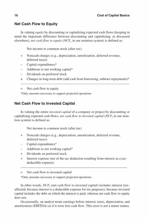
Net Cash Flow to Equity
In valuing equity by discounting or capitalizing expected cash flows (keeping inmind the important difference between discounting and capitalizing, as discussedelsewhere), net cash flow to equity (NCFe in our notation system) is defined as:
Net income to common stock (after tax)
+ Noncash charges (e.g., depreciation, amortization, deferred revenue,deferred taxes)
– Capital expenditures*
– Additions to net working capital*
– Dividends on preferred stock
± Changes in long-term debt (add cash from borrowing, subtract repayments)*
————————————————————————————————
= Net cash flow to equity
*Only amounts necessary to support projected operations
Net Cash Flow to Invested Capital
In valuing the entire invested capital of a company or project by discounting orcapitalizing expected cash flows, net cash flow to invested capital (NCFf in our nota-tion system) is defined as:
Net income to common stock (after tax)
+ Noncash charges (e.g., depreciation, amortization, deferred revenue,deferred taxes)
– Capital expenditures*
– Additions to net working capital*
+ Dividends on preferred stock
+ Interest expense (net of the tax deduction resulting from interest as a tax-deductible expense)
———————————————————————————————
= Net cash flow to invested capital
*Only amounts necessary to support projected operations
In other words, NCFf (net cash flow to invested capital) includes interest (tax-affected, because interest is a deductible expense for tax purposes), because investedcapital includes the debt on which the interest is paid, whereas net cash flow to equitydoes not.
Occasionally, an analyst treats earnings before interest, taxes, depreciation, andamortization (EBITDA) as if it were free cash flow. This error is not a minor matter,
16 Cost of Capital Basics
3953 P-03 8/29/02 2:19 PM Page 16
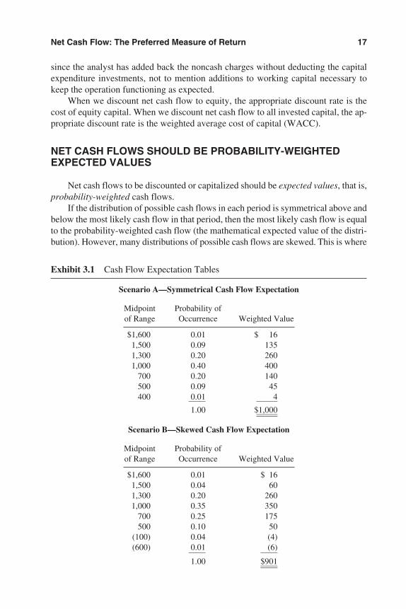
since the analyst has added back the noncash charges without deducting the capitalexpenditure investments, not to mention additions to working capital necessary tokeep the operation functioning as expected.
When we discount net cash flow to equity, the appropriate discount rate is thecost of equity capital. When we discount net cash flow to all invested capital, the ap-propriate discount rate is the weighted average cost of capital (WACC).
NET CASH FLOWS SHOULD BE PROBABILITY-WEIGHTEDEXPECTED VALUES
Net cash flows to be discounted or capitalized should be expected values, that is,probability-weighted cash flows.
If the distribution of possible cash flows in each period is symmetrical above andbelow the most likely cash flow in that period, then the most likely cash flow is equalto the probability-weighted cash flow (the mathematical expected value of the distri-bution). However, many distributions of possible cash flows are skewed. This is where
Net Cash Flow: The Preferred Measure of Return 17
Exhibit 3.1 Cash Flow Expectation Tables
Scenario A—Symmetrical Cash Flow Expectation
Midpoint Probability ofof Range Occurrence Weighted Value
$1,600 0.01 $ 161,500 0.09 1351,300 0.20 2601,000 0.40 400
700 0.20 140500 0.09 45400 0.01 4—–– ——–
1.00 $1,000——–——–
Scenario B—Skewed Cash Flow Expectation
Midpoint Probability ofof Range Occurrence Weighted Value
$1,600 0.01 $ 161,500 0.04 601,300 0.20 2601,000 0.35 350
700 0.25 175500 0.10 50
(100) 0.04 (4)(600) 0.01 (6)—–– –—–
1.00 $901–—––—–
3953 P-03 8/29/02 2:19 PM Page 17
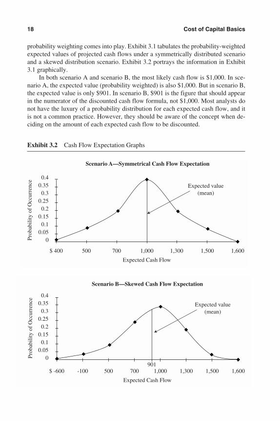
probability weighting comes into play. Exhibit 3.1 tabulates the probability-weightedexpected values of projected cash flows under a symmetrically distributed scenarioand a skewed distribution scenario. Exhibit 3.2 portrays the information in Exhibit3.1 graphically.
In both scenario A and scenario B, the most likely cash flow is $1,000. In sce-nario A, the expected value (probability weighted) is also $1,000. But in scenario B,the expected value is only $901. In scenario B, $901 is the figure that should appearin the numerator of the discounted cash flow formula, not $1,000. Most analysts donot have the luxury of a probability distribution for each expected cash flow, and itis not a common practice. However, they should be aware of the concept when de-ciding on the amount of each expected cash flow to be discounted.
18 Cost of Capital Basics
Exhibit 3.2 Cash Flow Expectation Graphs
Scenario A—Symmetrical Cash Flow Expectation
Expected Cash Flow
Expected value(mean)
Prob
abili
ty o
f O
ccur
renc
e
$ 400
0.40.350.3
0.250.2
0.150.1
0.050
500 700 1,000 1,300 1,500 1,600
Scenario B—Skewed Cash Flow Expectation
Expected Cash Flow
Expected value(mean)
Prob
abili
ty o
f O
ccur
renc
e
$ -600 -100 500 700901
1,000 1,300 1,500 1,600
0.40.350.3
0.250.2
0.150.1
0.050
3953 P-03 8/29/02 2:19 PM Page 18
WHY NET CASH FLOW IS THE PREFERRED MEASURE OFECONOMIC INCOME
There are two reasons why the financial community tends to focus on net cashflow as the preferred measure of economic income to be discounted by the opportunitycost of capital to estimate the net present value of an investment opportunity. They are:
1. Conceptual: It is what you really get (i.e., what an investor actually expects toreceive).
2. Empirical: It is the economic income measure for which we have the best his-torical data available to estimate a discount rate.
Conceptual Reason for Preferring Net Cash Flow
Net cash flow, as defined earlier, is that portion of the cash flow over which thecontrol owner has total discretion as to its disposal. It is not necessary to retain netcash flow to sustain the business; rather, it is available to be paid out to owners or usedfor any other desired purposes. This is the measure of economic income of greatestinterest to most investors.
Ibbotson clearly states the case for preferring what it terms “free cash flows” (i.e.,net cash flows after tax) as the appropriate economic income measure to discount:
There are several things to note about free cash flow. First, it is an after-tax concept.While the equation starts with earnings before interest and taxes (EBIT), this number istax-adjusted to get to an after-tax value. The equation starts with tax-adjusted EBIT be-cause we want to focus on cash flows independently of capital structure. We must there-fore start with earnings before interest expenses and then tax adjust those earnings.Secondly, pure accounting adjustments need to be added back into the analysis. It is forthis reason that depreciation expense and deferred tax expense are added back into theafter-tax EBIT. Finally, cash flows necessary to keep the company going forward mustbe subtracted from the equation. These cash flows represent necessary capital expendi-tures to maintain plant, property, and equipment or other capital expenditures that ariseout of the ordinary course of business. Another common subtraction is reflected inchanges in working capital. The assumption in most business valuation settings is thatthe entity in question will remain a long-term going concern that will grow over time.As companies grow, they accumulate additional accounts receivable and other workingcapital elements that require additional cash to support.
Free cash flow is the relevant cash flow stream because it represents the broadestlevel of earnings that can be generated by the asset. With free cash flow as the startingpoint, the owners of a firm can decide how much of the cash flow stream should be di-verted toward new ventures, capital expenditures, interest payments, and dividend pay-ments. It is incorrect to focus on earnings as the cash flow stream to be valued becauseearnings contain a number of accounting adjustments and already include the impact ofthe capital structure.1
Net Cash Flow: The Preferred Measure of Return 19
3953 P-03 8/29/02 2:19 PM Page 19
Empirical Reason for Preferring Net Cash Flow
If the Ibbotson Associates data are used to develop an equity discount rate—using either the build-up model or the Capital Asset Pricing Model (CAPM)—the dis-count rate is applicable to net cash flow available to the equity investor. This isbecause the Ibbotson return data have two components:
1. Dividends
2. Change in stock price
The investor receives the dividends, so their utilization is entirely at the investor’sdiscretion. The investor’s realization of the change in stock price is equally discre-tionary because the stocks are highly liquid (i.e., they can be sold at their market priceat any time, with the seller receiving the proceeds in cash within three business days).
SUMMARY
Net cash flow is the measure of economic income that most financial analysts pre-fer to use today when using the cost of capital for valuation or project selection. If valu-ing cash flows to equity, the discount rate should be the cost of equity capital. Ifvaluing cash flows to debt, the discount rate should be the cost of the debt capital.If valuing cash flows available for all invested capital, the discount rate should be theweighted average cost of capital (WACC).
There are two good reasons why financial analysts lean toward using net cashflow as the preferred measure of economic income when using cost of capital for val-uation or project selection:
1. Conceptually, it is the amount of discretionary money available to be distributedwithout disrupting the projected ongoing operations of the enterprise.
2. Empirically, it is the economic income measure for which the best historical datais available for estimating cost of equity capital.
Net cash flows should be measured as the mathematical expected value of theprobability-weighted distribution of expected outcomes for each projected period ofreturns, not the most likely value. In Chapter 5, we define risk by uncertainty of pos-sible outcomes, a definition intended to encompass the entire range of possible re-turns for each future period.
Note
1. Stocks, Bonds, Bills and Inflation, Valuation Edition 2002 Yearbook (Chicago: IbbotsonAssociates, 2002), 13. Used with permission. All rights reserved.
20 Cost of Capital Basics
3953 P-03 8/29/02 2:19 PM Page 20
21
Chapter 4
Discounting versusCapitalizingCapitalization FormulaExample: Valuing a Preferred StockFunctional Relationship between Discount Rate and Capitalization RateMajor Difference between Discounting and CapitalizingGordon Growth ModelCombining Discounting and Capitalizing (Two-stage Model)Equivalency of Discounting and Capitalizing ModelsMidyear Convention
Midyear Discounting ConventionMidyear Capitalization ConventionMidyear Convention in the Two-stage Model
Converting from After-tax Rate to Pretax RateConverting After-tax Capitalization Rate to Pretax Capitalization RateConverting After-tax Rate to Pretax Discount Rate
Summary
In the context of cost of capital applications, there is a very clear distinction be-tween a discount rate and a capitalization rate. The first two chapters explained thatthe cost of capital is used as a discount rate to discount a stream of future returns toa present value. This process is called discounting.
In discounting, we project all expected returns (cash flows or other measure ofeconomic income) from the subject investment to the respective class or classes ofcapital over the life of the investment. Thus, the percentage return that we call the dis-count rate represents the total compound rate of return that an investor in that classof investment expects to achieve over the life of the investment.
There is a related process for estimating present value, which we call capitaliz-ing. In capitalizing, instead of projecting all future returns on the investment to the re-spective class(es) of capital, we focus on the return of just one single period, usuallythe return expected in the first year immediately following the valuation date. We thendivide that single number by a divisor called the capitalization rate. This process iscalled capitalizing.
As will be seen, the process of capitalizing is really just a shorthand form of dis-counting, and the capitalization rate is actually a derivative of the discount rate. That
3953 P-04 8/29/02 2:20 PM Page 21
is, the capitalization rate, as used in the income approach to valuation or project selec-tion, is formed by derivation from the discount rate. (This differs from the marketapproach to valuation, where capitalization rates for various economic income mea-sures are observed directly in the marketplace.)
CAPITALIZATION FORMULA
Putting this concept into a formula, we have:
Formula 4.1
where:
PV = Present valueNCF1 = Net cash flow expected in the first period immediately following the
valuation datec = Capitalization rate
EXAMPLE: VALUING A PREFERRED STOCK
A simple example of applying Formula 4.1 uses a preferred stock for which a riskrating has been estimated. Let us make five assumptions:
1. The preferred stock pays dividends of $5 per share per year.
2. The preferred stock is issued in perpetuity and is not callable.
3. It pays dividends once a year, at the end of the year. (This, of course, is a simplify-ing assumption. Some privately owned preferred stocks pay only annually, butmost publicly traded preferred stocks pay dividends quarterly.)
4. As of the valuation date, the market yield for preferred stocks of the same riskgrade as the subject preferred stock is 10%. (We also must assume comparablerights, such as voting, liquidation preference, redemption, conversion, participa-tion, cumulative dividends, etc.)
5. There is no prospect of liquidation.
Note that the par value of the preferred stock is irrelevant, since the stock is issuedin perpetuity and there is no prospect of a liquidation. The entire cash flow an investorcan expect to receive over the life of the investment (perpetuity in this case) is the $5per-year per-share dividend.
Substituting numbers derived from the preceding assumptions into Formula 4.1produces:
PVNCF
c= 1
22 Cost of Capital Basics
3953 P-04 8/29/02 2:20 PM Page 22
Formula 4.2
In this example, the estimated fair market value of the subject preferred stock is$50 per share. That is the amount a willing buyer would expect to pay and a willingseller would expect to receive (before considering any transaction costs).
FUNCTIONAL RELATIONSHIP BETWEEN DISCOUNT RATE AND CAPITALIZATION RATE
The preceding example presented the simplest possible scenario in which to applythe cost of capital through the capitalization method: a fixed cash flow stream in per-petuity. This is the one unique situation in which the discount rate (cost of capital)equals the capitalization rate. The discount rate equals the capitalization rate becauseno growth or decline in the investor’s cash flow is expected. But most real-world in-vestments are not quite that simple.
In the case of an investment in common stock, a partnership interest, or a capi-tal budgeting project in an operating company, investors often are expecting somelevel of growth over time in the cash flows available to pay dividends or partnershipwithdrawals. Even if unit volume is expected to remain constant (i.e., no real growth),investors still might expect cash flows to grow at a rate approximating expected in-flation. If the expected annually compounded rate of growth is stable and sustainableover a long period of time, then the discount rate (cost of capital) can be converted toa capitalization rate.
As stated earlier, the capitalization rate is a function of the discount rate. This ob-viously raises the question: What is the functional relationship between the discountrate and the capitalization rate?
Assuming stable long-term growth in the cash flows available to the investmentbeing valued, the capitalization rate equals the discount rate minus the expected long-term growth rate. In a formula, this functional relationship can be stated as:
Formula 4.3
c = k – g
where:
c = Capitalization ratek = Discount rate (cost of capital) for the subject investmentg = Expected long-term sustainable growth rate in the cash flow available
to the subject investment
The critical assumption in this formula is that the growth in the return availableto the capital is relatively constant over the long term (technically in perpetuity).
Caveat: Note carefully the phrase “return available to the capital.” This does notinclude growth in overall company cash flows that are dependent on future capital in-
PV =
=
$ .
.$ .
5 00
0 1050 00
Discounting versus Capitalizing 23
3953 P-04 8/29/02 2:20 PM Page 23
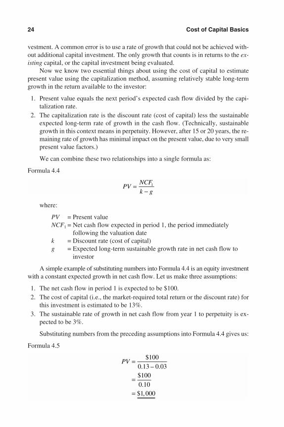
vestment. A common error is to use a rate of growth that could not be achieved with-out additional capital investment. The only growth that counts is in returns to the ex-isting capital, or the capital investment being evaluated.
Now we know two essential things about using the cost of capital to estimatepresent value using the capitalization method, assuming relatively stable long-termgrowth in the return available to the investor:
1. Present value equals the next period’s expected cash flow divided by the capi-talization rate.
2. The capitalization rate is the discount rate (cost of capital) less the sustainableexpected long-term rate of growth in the cash flow. (Technically, sustainablegrowth in this context means in perpetuity. However, after 15 or 20 years, the re-maining rate of growth has minimal impact on the present value, due to very smallpresent value factors.)
We can combine these two relationships into a single formula as:
Formula 4.4
where:
PV = Present valueNCF1 = Net cash flow expected in period 1, the period immediately
following the valuation datek = Discount rate (cost of capital)g = Expected long-term sustainable growth rate in net cash flow to
investor
A simple example of substituting numbers into Formula 4.4 is an equity investmentwith a constant expected growth in net cash flow. Let us make three assumptions:
1. The net cash flow in period 1 is expected to be $100.2. The cost of capital (i.e., the market-required total return or the discount rate) for
this investment is estimated to be 13%.3. The sustainable rate of growth in net cash flow from year 1 to perpetuity is ex-
pected to be 3%.
Substituting numbers from the preceding assumptions into Formula 4.4 gives us:
Formula 4.5
PV =
=
=
$
. – .$
.$ ,
100
0 13 0 03100
0 101 000
PVNCF
k g=
−1
24 Cost of Capital Basics
3953 P-04 8/29/02 2:20 PM Page 24
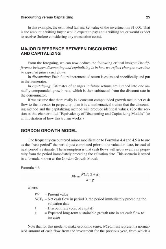
In this example, the estimated fair market value of the investment is $1,000. Thatis the amount a willing buyer would expect to pay and a willing seller would expectto receive (before considering any transaction costs).
MAJOR DIFFERENCE BETWEEN DISCOUNTING AND CAPITALIZING
From the foregoing, we can now deduce the following critical insight: The dif-ference between discounting and capitalizing is in how we reflect changes over timein expected future cash flows.
In discounting: Each future increment of return is estimated specifically and putin the numerator.
In capitalizing: Estimates of changes in future returns are lumped into one an-nually compounded growth rate, which is then subtracted from the discount rate inthe denominator.
If we assume that there really is a constant compounded growth rate in net cashflow to the investor in perpetuity, then it is a mathematical truism that the discount-ing method and the capitalizing method will produce identical values. (See the sec-tion in this chapter titled “Equivalency of Discounting and Capitalizing Models” foran illustration of how this truism works.)
GORDON GROWTH MODEL
One frequently encountered minor modification to Formulas 4.4 and 4.5 is to useas the “base period” the period just completed prior to the valuation date, instead ofnext period’s estimate. The assumption is that cash flows will grow evenly in perpe-tuity from the period immediately preceding the valuation date. This scenario is statedin a formula known as the Gordon Growth Model:
Formula 4.6
where:
PV = Present valueNCF0 = Net cash flow in period 0, the period immediately preceding the
valuation datek = Discount rate (cost of capital)g = Expected long-term sustainable growth rate in net cash flow to
investor
Note that for this model to make economic sense, NCF0 must represent a normal-ized amount of cash flow from the investment for the previous year, from which a
PVNCF g
k g= +
−0 1( )
Discounting versus Capitalizing 25
3953 P-04 8/29/02 2:20 PM Page 25
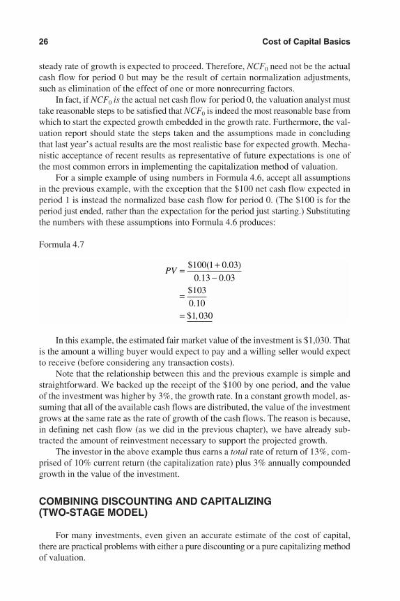
steady rate of growth is expected to proceed. Therefore, NCF0 need not be the actualcash flow for period 0 but may be the result of certain normalization adjustments,such as elimination of the effect of one or more nonrecurring factors.
In fact, if NCF0 is the actual net cash flow for period 0, the valuation analyst musttake reasonable steps to be satisfied that NCF0 is indeed the most reasonable base fromwhich to start the expected growth embedded in the growth rate. Furthermore, the val-uation report should state the steps taken and the assumptions made in concludingthat last year’s actual results are the most realistic base for expected growth. Mecha-nistic acceptance of recent results as representative of future expectations is one ofthe most common errors in implementing the capitalization method of valuation.
For a simple example of using numbers in Formula 4.6, accept all assumptionsin the previous example, with the exception that the $100 net cash flow expected inperiod 1 is instead the normalized base cash flow for period 0. (The $100 is for theperiod just ended, rather than the expectation for the period just starting.) Substitutingthe numbers with these assumptions into Formula 4.6 produces:
Formula 4.7
In this example, the estimated fair market value of the investment is $1,030. Thatis the amount a willing buyer would expect to pay and a willing seller would expectto receive (before considering any transaction costs).
Note that the relationship between this and the previous example is simple andstraightforward. We backed up the receipt of the $100 by one period, and the valueof the investment was higher by 3%, the growth rate. In a constant growth model, as-suming that all of the available cash flows are distributed, the value of the investmentgrows at the same rate as the rate of growth of the cash flows. The reason is because,in defining net cash flow (as we did in the previous chapter), we have already sub-tracted the amount of reinvestment necessary to support the projected growth.
The investor in the above example thus earns a total rate of return of 13%, com-prised of 10% current return (the capitalization rate) plus 3% annually compoundedgrowth in the value of the investment.
COMBINING DISCOUNTING AND CAPITALIZING (TWO-STAGE MODEL)
For many investments, even given an accurate estimate of the cost of capital,there are practical problems with either a pure discounting or a pure capitalizing methodof valuation.
PV = +−
=
=
$ ( . )
. .$
.$ ,
100 1 0 03
0 13 0 03103
0 101 030
26 Cost of Capital Basics
3953 P-04 8/29/02 2:20 PM Page 26
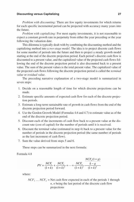
Problem with discounting: There are few equity investments for which returnsfor each specific incremental period can be projected with accuracy many years intothe future.
Problem with capitalizing: For most equity investments, it is not reasonable toexpect a constant growth rate in perpetuity from either the year preceding or the yearfollowing the valuation date.
This dilemma is typically dealt with by combining the discounting method and thecapitalizing method into a two-stage model. The idea is to project discrete cash flowsfor some number of periods into the future and then to project a steady growth modelstarting at the end of the discrete projection period. Each period’s discrete cash flow isdiscounted to a present value, and the capitalized value of the projected cash flows fol-lowing the end of the discrete projection period is also discounted back to a presentvalue. The sum of the present values is the total present value. The capitalized value ofthe projected cash flows following the discrete projection period is called the terminalvalue or residual value.
The preceding narrative explanation of a two-stage model is summarized inseven steps:
1. Decide on a reasonable length of time for which discrete projections can bemade.
2. Estimate specific amounts of expected cash flow for each of the discrete projec-tion periods.
3. Estimate a long-term sustainable rate of growth in cash flows from the end of thediscrete projection period forward.
4. Use the Gordon Growth Model (Formulas 4.6 and 4.7) to estimate value as of theend of the discrete projection period.
5. Discount each of the increments of cash flow back to a present value at the dis-count rate (cost of capital) for the number of periods until it is received.
6. Discount the terminal value (estimated in step 4) back to a present value for thenumber of periods in the discrete projection period (the same number of periodsas the last increment of cash flow).
7. Sum the value derived from steps 5 and 6.
These steps can be summarized in the next formula:
Formula 4.8
where:
NCF1 … NCFn = Net cash flow expected in each of the periods 1 throughn, n being the last period of the discrete cash flowprojections
PVNCF
k
NCF
k
NCF
k
NCF g
k gk
nn
n
n=+
++
+ ++
+−
+1 2
21 1 1
1
1( ) ( ) ( )
( )
( )L
Discounting versus Capitalizing 27
3953 P-04 8/29/02 2:20 PM Page 27
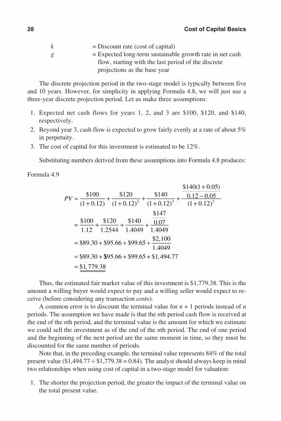
k = Discount rate (cost of capital)g = Expected long-term sustainable growth rate in net cash
flow, starting with the last period of the discreteprojections as the base year
The discrete projection period in the two-stage model is typically between fiveand 10 years. However, for simplicity in applying Formula 4.8, we will just use athree-year discrete projection period. Let us make three assumptions:
1. Expected net cash flows for years 1, 2, and 3 are $100, $120, and $140,respectively.
2. Beyond year 3, cash flow is expected to grow fairly evenly at a rate of about 5%in perpetuity.
3. The cost of capital for this investment is estimated to be 12%.
Substituting numbers derived from these assumptions into Formula 4.8 produces:
Formula 4.9
Thus, the estimated fair market value of this investment is $1,779.38. This is theamount a willing buyer would expect to pay and a willing seller would expect to re-ceive (before considering any transaction costs).
A common error is to discount the terminal value for n + 1 periods instead of nperiods. The assumption we have made is that the nth period cash flow is received atthe end of the nth period, and the terminal value is the amount for which we estimatewe could sell the investment as of the end of the nth period. The end of one periodand the beginning of the next period are the same moment in time, so they must bediscounted for the same number of periods.
Note that, in the preceding example, the terminal value represents 84% of the totalpresent value ($1,494.77 ÷ $1,779.38 = 0.84). The analyst should always keep in mindtwo relationships when using cost of capital in a two-stage model for valuation:
1. The shorter the projection period, the greater the impact of the terminal value onthe total present value.
PV =+
++
++
+
+−
+
= + + +
= + + +
= +
$
( . )
$
( . )
$
( . )
$ ( . )
. .( . )
$
.
$
.
$
.
$
..
$ . $ . $ .$ ,
.$ .
100
1 0 12
120
1 0 12
140
1 0 12
140 1 0 05
0 12 0 051 0 12
100
1 12
120
1 2544
140
1 4049
147
0 071 4049
89 30 95 66 99 652 100
1 404989 30
2 3 3
$$ . $ . $ , .
$ , .
95 66 99 65 1 494 77
1 779 38
+ +=
28 Cost of Capital Basics
3953 P-04 8/29/02 2:20 PM Page 28
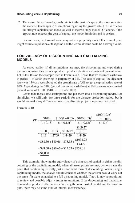
2. The closer the estimated growth rate is to the cost of capital, the more sensitivethe model is to changes in assumptions regarding the growth rate. (This is true forthe straight capitalization model as well as the two-stage model.) Of course, if thegrowth rate exceeds the cost of capital, the model implodes and is useless.
In some cases, the terminal value may not be a perpetuity model. For example, onemight assume liquidation at that point, and the terminal value could be a salvage value.
EQUIVALENCY OF DISCOUNTING AND CAPITALIZINGMODELS
As stated earlier, if all assumptions are met, the discounting and capitalizingmethods of using the cost of capital will produce identical estimates of present value.Let us test this on the example used in Formula 4.5. Recall that we assumed cash flowin period 1 of $100, growing in perpetuity at 3%. The cost of capital (the discountrate) was 13%, so we subtracted the growth rate of 3% to get a capitalization rate of10%. Capitalizing the $100 (period 1 expected cash flow) at 10% gave us an estimatedpresent value of $1,000 ($100 ÷ 0.10 = $1,000).
Let us take these same assumptions and put them into a discounting model. Forsimplicity, we will only use three periods for the discrete projection period, but itwould not make any difference how many discrete projection periods we used.
Formula 4.10
This example, showing the equivalency of using cost of capital in either the dis-counting or the capitalizing model, when all assumptions are met, demonstrates thepoint that capitalizing is really just a shorthand form of discounting. When using acapitalizing model, the analyst should consider whether the answer would work outthe same if it were expanded to a full discounting model. If not, it may be propitiousto review and possibly adjust certain assumptions. If the discounting and capitaliza-tion models produce different answers using the same cost of capital and the same in-puts, there may be some kind of internal inconsistency.
PV =+
+ ++
++
+ −
= + + +
= + + +
$
( . )
$ ( . )
( . )
$ ( . )
( . )
$ ( . )
. .( . )
$
.
$
.
$ .
.
$ .
..
$ . $ . $ .
100
1 0 13
100 1 0 03
1 0 13
100 1 03
1 0 13
100 1 03
0 13 0 031 13
100
1 13
103
1 2769
106 09
1 4429
109 27
0 101 4429
88 50 80 66 73 53
2
2
3
3
3
$$ .
.$ . $ . $ . $ .
$ ,
1092 73
1 442988 50 80 66 73 53 757 31
1 000
= + + +=
Discounting versus Capitalizing 29
3953 P-04 8/29/02 2:20 PM Page 29
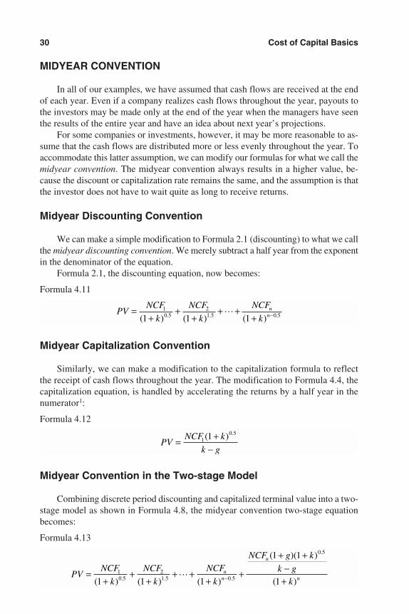
MIDYEAR CONVENTION
In all of our examples, we have assumed that cash flows are received at the endof each year. Even if a company realizes cash flows throughout the year, payouts tothe investors may be made only at the end of the year when the managers have seenthe results of the entire year and have an idea about next year’s projections.
For some companies or investments, however, it may be more reasonable to as-sume that the cash flows are distributed more or less evenly throughout the year. Toaccommodate this latter assumption, we can modify our formulas for what we call themidyear convention. The midyear convention always results in a higher value, be-cause the discount or capitalization rate remains the same, and the assumption is thatthe investor does not have to wait quite as long to receive returns.
Midyear Discounting Convention
We can make a simple modification to Formula 2.1 (discounting) to what we callthe midyear discounting convention. We merely subtract a half year from the exponentin the denominator of the equation.
Formula 2.1, the discounting equation, now becomes:
Formula 4.11
Midyear Capitalization Convention
Similarly, we can make a modification to the capitalization formula to reflectthe receipt of cash flows throughout the year. The modification to Formula 4.4, thecapitalization equation, is handled by accelerating the returns by a half year in thenumerator1:
Formula 4.12
Midyear Convention in the Two-stage Model
Combining discrete period discounting and capitalized terminal value into a two-stage model as shown in Formula 4.8, the midyear convention two-stage equationbecomes:
Formula 4.13
PVNCF
k
NCF
k
NCF
k
NCF g k
k gk
nn
n
n=+
++
+ ++
+
+ +−
+−10 5
21 5 0 5
0 5
1 1 1
1 1
1( ) ( ) ( )
( )( )
( ). . .
.
L
PVNCF k
k g= +
−1
0 51( ) .
PVNCF
k
NCF
k
NCF
kn
n=+
++
+ ++ −
10 5
21 5 0 51 1 1( ) ( ) ( ). . .L
30 Cost of Capital Basics
3953 P-04 8/29/02 2:20 PM Page 30
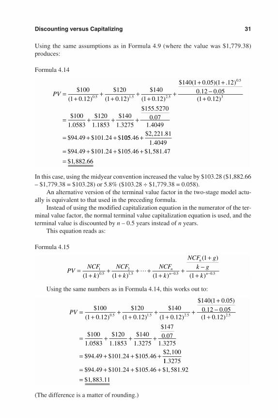
Using the same assumptions as in Formula 4.9 (where the value was $1,779.38)produces:
Formula 4.14
In this case, using the midyear convention increased the value by $103.28 ($1,882.66– $1,779.38 = $103.28) or 5.8% ($103.28 ÷ $1,779.38 = 0.058).
An alternative version of the terminal value factor in the two-stage model actu-ally is equivalent to that used in the preceding formula.
Instead of using the modified capitalization equation in the numerator of the ter-minal value factor, the normal terminal value capitalization equation is used, and theterminal value is discounted by n – 0.5 years instead of n years.
This equation reads as:
Formula 4.15
Using the same numbers as in Formula 4.14, this works out to:
(The difference is a matter of rounding.)
PV =+
++
++
+
+−
+
= + + +
= + + +
$
( . )
$
( . )
$
( . )
$ ( . )
. .( . )
$
.
$
.
$
.
$
..
$ . $ . $ .$ ,
. . . .
100
1 0 12
120
1 0 12
140
1 0 12
140 1 0 05
0 12 0 051 0 12
100
1 0583
120
1 1853
140
1 3275
147
0 071 3275
94 49 101 24 105 462 100
0 5 1 5 2 5 2 5
11 327594 49 101 24 105 46 1 581 92
1 883 11
.$ . $ . $ . $ , .
$ , .
= + + +=
PVNCF
k
NCF
k
NCF
k
NCF g
k gk
nn
n
n=+
++
+ ++
+
+−
+− −10 5
21 5 0 5 0 51 1 1
1
1( ) ( ) ( )
( )
( ). . . .L
PV =+
++
++
+
+ +−
+
= + + +
= + +
$
( . )
$
( . )
$
( . )
$ ( . )( . ). .
( . )
$
.
$
.
$
.
$ ..
.
$ . $ . $
. . .
.
100
1 0 12
120
1 0 12
140
1 0 12
140 1 0 05 1 120 12 0 051 0 12
100
1 0583
120
1 1853
140
1 3275
155 52700 07
1 4049
94 49 101 24
0 5 1 5 2 5
0 5
3
105105 462 221 81
1 404994 49 101 24 105 46 1 581 47
1 882 66
.$ , .
.$ . $ . $ . $ , .
$ , .
+
= + + +=
Discounting versus Capitalizing 31
3953 P-04 8/29/02 2:20 PM Page 31
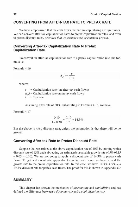
CONVERTING FROM AFTER-TAX RATE TO PRETAX RATE
We have emphasized that the cash flows that we are capitalizing are after taxes.We can convert after-tax capitalization rates to pretax capitalization rates, and evento pretax discount rates, provided that we assume zero or constant growth.
Converting After-tax Capitalization Rate to Pretax Capitalization Rate
To convert an after-tax capitalization rate to a pretax capitalization rate, the for-mula is:
Formula 4.16
where:
c = Capitalization rate (on after-tax cash flows)c(pt) = Capitalization rate on pretax cash flowst = Tax rate
Assuming a tax rate of 30%, substituting in Formula 4.16, we have:
Formula 4.17
But the above is not a discount rate, unless the assumption is that there will be nogrowth.
Converting After-tax Rate to Pretax Discount Rate
Suppose that we arrived at the above capitalization rate of 10% by starting with adiscount rate of 15% and subtracting an estimated sustainable growth rate of 5% (0.15– 0.05 = 0.10). We are not going to apply a discount rate of 14.3% to pretax cashflows! To get a discount rate applicable to pretax cash flows, we have to add thegrowth rate to the pretax capitalization rate. In this case, we have 14.3% + 5% = a19.3% discount rate for pretax cash flows. The proof for this is shown in Appendix G.2
SUMMARY
This chapter has shown the mechanics of discounting and capitalizing and hasdefined the difference between a discount rate and a capitalization rate.
0 10
1 0 30
0 10
0 7014 3
.
– .
.
.. %= =
cc
tpt( )–
=1
32 Cost of Capital Basics
3953 P-04 8/29/02 2:20 PM Page 32
It has shown that capitalizing is merely a short-form version of discounting. Theessential difference between the discounting method and the capitalizing method ishow changes in expected cash flows over time are reflected in the respective formu-las. All things being equal, the discounting method and the capitalizing method willyield identical results. However, the validity of the capitalizing method in the incomeapproach to valuation depends on the assumption that the difference between the dis-count rate and the capitalization rate represents a long-term average rate of growth inthe income variable being capitalized.
Because many companies are likely to expect near-term changes in levels oftheir returns that are not expected to be representative of longer-term expectations,many analysts use a combination of discounting and capitalizing for valuation. To ac-complish this, they implement five steps:
1. Project discrete amounts of return for some period of years until the company isexpected to reach a stabilized level from which relatively constant growth maybe expected to proceed.
2. Use the Gordon Growth Model to estimate a “terminal value” as of the end of thediscrete projection period.
3. Discount each discrete projected cash flow to a present value at the cost of cap-ital for the number of periods until it is expected to be received.
4. Discount the terminal value to a present value at the cost of capital for the num-ber of periods in the discrete projection period (the beginning of the assumed sta-ble growth period).
5. Add the values from steps 3 and 4.
Most discounting and capitalization formulas reflect the implicit assumption thatinvestors will realize their cash flows at the end of each year. If it is assumed thatinvestors will receive cash flows more or less evenly throughout the year, the for-mulas can be modified by the midyear convention.
Notes
1. Proof of the accuracy of this method was presented in Todd A. Kaltman, “CapitalizationUsing a Mid-Year Convention,” Business Valuation Review (December 1995): 178–182.
2. This was first demonstrated in Mary Ann Lerch, “Pretax/Aftertax Conversion Formula forCapitalization Rates and Cash Flow Discount Rates,” Business Valuation Review (March1990): 18–22.
Discounting versus Capitalizing 33
3953 P-04 8/29/02 2:20 PM Page 33
34
Chapter 5
Relationship between Riskand the Cost of CapitalDefining RiskTypes of Risk
Maturity RiskSystematic RiskUnsystematic Risk
How Risk Impacts the Cost of CapitalCost of Equity CapitalCost of Conventional Debt and Preferred Equity CapitalCost of Overall Invested CapitalSummary
The cost of capital for any given investment is a combination of two basic factors1:
1. A risk-free rate. By “risk-free rate” we mean a rate of return that is available inthe market on an investment that is free of default risk, usually the yield to ma-turity on a U.S. government security.
2. A premium for risk. An expected amount of return over and above the risk-freerate to compensate the investor for accepting risk.
Quantifying the amount by which risk affects the cost of capital for any particularcompany or investment is arguably one of the most difficult analyses in the field ofcorporate finance, including valuation and capital budgeting.
DEFINING RISK
Probably the most widely accepted definition of risk in the context of businessvaluation is the degree of uncertainty as to the realization of expected future economicincome.2 This means uncertainty as to both the amounts and the timing of expectedincome. Note that the definition implies as the reference point expected returns. Byexpected returns, in a technical sense, we mean the expected value (mean average) ofthe probability distribution of possible returns for each forecast period. This conceptwas explained in Chapter 3 in the discussion of net cash flow. The point to understand
3953 P-05 8/29/02 2:20 PM Page 34
here is that the uncertainty encompasses the full distribution of possible returns foreach period both above and below the expected value.
Inasmuch as uncertainty is within the mind of each individual investor, we can-not measure the risk directly. Consequently, participants in the financial markets havedeveloped ways of measuring factors that investors normally would consider in theireffort to incorporate risk into their required rate of return.
TYPES OF RISK
Although risk arises from many sources, this chapter addresses risk in the eco-nomic sense, as used in the conventional methods of estimating cost of capital. In thiscontext, capital market theory divides risk into three components:
1. Maturity risk (also called horizon risk or interest rate risk)
2. Systematic risk (also called market risk)
3. Unsystematic risk (sometimes called company risk, specific risk, or residual risk)
Maturity Risk
Maturity risk (also called horizon risk or interest rate risk) is the risk that the valueof the investment may increase or decrease because of changes in the general level ofinterest rates. The longer the term of an investment, the greater the maturity risk. Forexample, market prices of long-term bonds fluctuate much more in response to changesin levels of interest rates than do short-term bonds or notes. When we refer to the yieldsof U.S. government bonds as riskless rates, we mean that we regard them as free fromthe prospect of default, but we recognize that they do incorporate maturity risk: Thelonger the maturity, the greater the susceptibility to change in market price in responseto changes in market rates of interest. In regard to interest rates, much of the uncertaintyderives from the uncertainty of future inflation levels.
Systematic Risk
Systematic risk (also called market risk) is the uncertainty of future returns be-cause of the sensitivity of the return on a subject investment to movements in returnsfor the investment market as a whole. Although this is a broad conceptual definition,in practical application the investment market as a whole is generally limited to theU.S. equity markets and is typically measured by returns on either the New York StockExchange (NYSE) Composite Index or the Standard & Poor’s (S&P) 500 Index.
Some theoreticians say that the only risk the capital markets reward with an ex-pected premium rate of return is systematic risk, because unsystematic risk can be elim-inated by holding a well-diversified portfolio of investments. Although this may betrue for active publicly traded securities, it generally is not practical to hold a portfolio
Relationship between Risk and the Cost of Capital 35
3953 P-05 8/29/02 2:20 PM Page 35
of closely held companies that is diversified enough to eliminate all risk except thatof the market itself.
As we cover the chapters on the various methods of estimating the cost of capi-tal, we will see that systematic risk is a factor specifically measured for a particularcompany or industry in some methods, but not at all or not necessarily in others. Sys-tematic risk is taken into consideration in the Capital Asset Pricing Model (CAPM),which is the subject of Chapter 9. It is commonly measured by a factor called beta,which attempts to measure the sensitivity of the returns realized by a company or anindustry to movements in returns of “the market,” usually defined as either the NYSEComposite Index or the S&P 500 Index.
Unsystematic Risk
Unsystematic risk (also called specific risk or residual risk) is the uncertainty ofexpected returns arising from factors other than the market itself. These factors typi-cally include characteristics of the industry and the individual company. In internationalinvesting, they also can include characteristics of a particular country.
Much of the unsystematic risk of an investment may be captured in the size pre-mium, which is the subject of Chapter 11. Fully capturing unsystematic risk in the dis-count rate requires analysis of the company, in comparison with other companies,which is also discussed in Chapter 11. However, while the size premium captures manyrisk factors, the analyst must be careful to capture all the risk factors and at the sametime avoid double-counting.
HOW RISK IMPACTS THE COST OF CAPITAL
As noted earlier, the cost of capital (the expected rate of return that the market re-quires to attract money to the subject investment) has two components3:
1. A riskless rate
2. A risk premium
As the market’s perception of the degree of risk of an investment increases, the rateof return that the market requires (the discount rate) increases. The higher the mar-ket’s required rate of return, the lower the present value of the investment.
Risk is the ultimate concern to investors. The riskless rate compensates investorsfor renting out their money, so to speak; that is, for delaying consumption over somefuture time period and receiving back dollars with less purchasing power. This com-ponent of the cost of capital is readily observable in the marketplace and generallydiffers from one investment to another only to the extent of the time horizon (matu-rity) selected for measurement of the riskless rate.
The risk premium, however, is due to the uncertainty of expected returns. It ismuch harder to estimate and also varies widely from one prospective capital investment
36 Cost of Capital Basics
3953 P-05 8/29/02 2:20 PM Page 36
to another. We could say that the market abhors uncertainty and consequently demandsa high price (in terms of required rate of return or cost of capital) to accept uncertainty.Since uncertainty as to timing and amounts of future receipts is greatest for equity in-vestors, the high risk forces equity as a class to have the highest cost of capital. Therisk premium varies greatly from one company or project to another, but for mostsmaller companies the risk premium component of the cost of capital is greater than theriskless rate component.
COST OF EQUITY CAPITAL
When using either the build-up method (Chapter 8) or the Capital Asset PricingModel (CAPM) (Chapter 9), we estimate one or more components of a risk premiumand add the total risk premium to the riskless rate in order to estimate the cost of eq-uity capital.
When using publicly traded stock data to estimate the cost of equity capital—thediscounted cash flow (DCF) method (Chapter 12)—we get a total cost of equity cap-ital without any explicit breakdown regarding how much of it is attributable to a risk-less rate and how much is attributable to the risk premium.
COST OF CONVENTIONAL DEBT AND PREFERRED EQUITY CAPITAL
The cost of debt and preferred stock capital generally depends on risk factorsidentified by fixed income rating services, such as Standard & Poor’s (now a divisionof McGraw-Hill) and Moody’s (now published by Mergent’s, Inc.). The rates of returnfor securities with comparable risk factors generally can be observed in the market.4
COST OF OVERALL INVESTED CAPITAL
The cost of total invested capital is a blending of the costs of each component,called the weighted average cost of capital (WACC). Chapter 6 discusses each com-ponent in the capital structure, and Chapter 7 addresses the weighted average cost ofcapital.
SUMMARY
The cost of capital is a function of the market’s risk-free rate plus a premium forthe risk associated with the investment. Risk is the degree of uncertainty regarding therealization of the expected returns from the investment.
Most analysts choose to use a long-term government security as a proxy for the“risk-free” rate. It is assumed that this rate is free of default risk, but it is recognized
Relationship between Risk and the Cost of Capital 37
3953 P-05 8/29/02 2:20 PM Page 37
that it includes interest rate risk; that is, the market value of the principal will changewith changes in the general level of interest rates.
In an economic sense, the market distinguishes between systematic risk and un-systematic risk. Systematic risk is the sensitivity of returns on the subject investmentto returns on the overall market. Unsystematic risk is unique to the subject companyor industry as opposed to the market as a whole.
Risk impacts the cost of each of the components of capital: debt, senior equity,and common equity. Because risk has an impact on each capital component, it alsohas an impact on the weighted average cost of capital.
As risk increases, the cost of capital increases, and value decreases. Because riskcannot be observed directly in the market, it must be estimated. The impact of risk onthe cost of capital is at once one of the most essential and one of the most difficultanalyses in corporate finance and investments.
Notes
1. A third factor is liquidity, but that is usually treated as a separate adjustment, as discussedin Chapter 16.
2. Shannon P. Pratt, Robert F. Reilly, and Robert P. Schweihs, Valuing a Business: The Analy-sis and Appraisal of Closely Held Companies, 4th ed. (New York: McGraw-Hill, 2000), 44.
3. As noted in note 1, a third element—lack of marketability or liquidity—may be embeddedin the discount rate, but more often it is treated as a separate adjustment to value. This iscovered in Chapter 16.
4. This text deals primarily with the cost of equity and the weighted average cost of capital.For detailed discussions on cost of debt and cost of preferred equity, see Chapters 23 and24 respectively, in Pratt, Reilly, and Schweihs, Valuing a Business.
38 Cost of Capital Basics
3953 P-05 8/29/02 2:20 PM Page 38
39
Chapter 6
Cost Components of aCompany’s Capital StructureDebt
Tax Effect Lowers Cost of DebtPersonal Guarantees
Preferred EquityConvertible Debt or Preferred StockCommon Stock or Partnership InterestsSummary
The capital structure of many companies includes two or more components,each of which has its own cost of capital. Such companies may be said to have a com-plex capital structure. The major components commonly found are:
• Debt
• Preferred stock
• Common stock or partnership interests
Similarly, a project being considered in a capital budgeting decision may be fi-nanced by multiple components of capital.
In a complex capital structure, each of these general components may have sub-components, and each subcomponent may have a different cost of capital. In addition,there may be hybrid or special securities, such as convertible debt or preferred stock,warrants, options, or leases.
Ultimately, a company’s or project’s overall cost of capital is a result of the blend-ing of the individual costs of each of these components. This chapter briefly discusseseach of the capital structure components, and Chapter 7 shows the process of blendingthem into a company’s or project’s overall cost of capital, which is called the weightedaverage cost of capital (WACC).
Estimation of the costs of conventional fixed-income components of the capitalstructure, that is, straight debt and preferred stock, is relatively straightforward, becausecosts of capital for securities of comparable risk usually are directly observable in themarket and the company’s actual embedded cost is often at or very close to current mar-ket rates. Although there can be many controversies surrounding costs of fixed incomecapital, especially if unusual provisions exist, we discuss these components only briefly
3953 P-06 8/29/02 2:21 PM Page 39
here. The rest of this book deals primarily with the critically important but highly elu-sive and controversial issue of the cost of equity.
DEBT
Conceptually, only long-term liabilities are included in a capital structure. How-ever, many closely held companies, especially smaller ones, use what is technicallyshort-term interest-bearing debt as if it were long-term debt. In these cases, it becomesa matter of the analyst’s judgment whether to reclassify the short-term debt as long-term debt and include it in the capital structure for the purpose of estimating the com-pany’s overall cost of capital (weighted average cost of capital).
Usually the cost of debt is equivalent to the company’s interest expense (after taxeffect) and is readily ascertainable from the footnotes to the company’s financial state-ments (if the company has either audited or reviewed statements or compiled statementswith footnote information). If the rate the company is paying is not a current market rate(e.g., long-term debt issued at a time when market rates were significantly different),then the analyst should estimate what a current market rate would be for that compo-nent of the company’s capital structure.
Standard & Poor’s (now a division of McGraw-Hill) publishes debt rating criteriaalong with the Standard & Poor’s Bond Guide. The analyst can see where the invest-ment would fit within the bond rating system, then check the financial press to findthe yields for the estimated rating.1 The analyst should consider that smaller companiesmay have higher costs of debt than larger companies. Also, smaller companies maynot be able to borrow as high a proportion of their capital structure as larger companies.Some companies have more than one class of debt, each with its own cost of debtcapital.
The relevant market “yield” is either the yield to maturity or the yield-to-call date.Either of these is the total return the debt holder expects to receive over the life of thedebt instrument, including current yield and any appreciation or depreciation from themarket price, to the redemption of the debt at either its maturity or call date, if callable.If the stated interest rate is above current market rates, the bond would be expectedto sell at a premium, and the yield-to-call date usually would be the appropriate yield,because it probably would be in the issuer’s best interest to call it (redeem it) as soonas possible and refinance it at a lower interest cost. If the stated interest rate is belowcurrent market rates, then it usually would not be attractive to the company to call it,and the yield to maturity would be the most appropriate rate.
Tax Effect Lowers Cost of Debt
Because interest expense on debt is a tax-deductible expense to a company, the netcost of debt to the company is the interest paid less the tax savings resulting from thedeductible interest payment. This cost of debt can be expressed by the next formula:
40 Cost of Capital Basics
3953 P-06 8/29/02 2:21 PM Page 40
Formula 6.1
kd = kd(pt)(1 – t)
where:
kd(pt) = Rate of interest on debtkd = Discount rate for debt (the company’s after-tax cost of debt capital)t = Tax rate (expressed as a percentage of pretax income)
For decision-making purposes, most corporate finance theoreticians recommendusing the marginal tax rate (the rate of tax paid on the last incremental dollar of tax-able income) if that differs from the company’s effective tax rate.2 That makes sense,since the marginal rate will be the cost incurred as a result of the investment. How-ever, the focus should be on the marginal rate over the life of the investment, if thatis different from the marginal cost incurred initially.
Personal Guarantees
When estimating the cost of private company debt, the analyst should ascertainwhether the debt is secured by personal guarantees. If so, this is an additional cost ofdebt that is not reflected directly in the financial statements (or, in some cases, mightnot even be disclosed). Such guarantees would justify an upward adjustment in thecompany’s cost of debt. The author is not aware of any published studies to helpquantify this factor. Therefore, it becomes a subjective adjustment on the part of theanalyst.3
In the late 1990s, insurance companies offered guarantees on seller financing. Thatis, when a company was sold with some percentage of the price as a down payment andthe buyer gave the seller a promissory note for the balance (a common procedure in thesale of small businesses and professional practices), the insurance company wouldguarantee the note to the seller. The required down payment was at least 30% of thepurchase price, and the premium was about 3% of the face value of the note. So perhaps3% is as good a guide as can be found for adding to the cost of debt to reflect personalguarantees.
PREFERRED EQUITY
If the capital structure includes preferred equity, the yield rate can be used as thecost of that component. If the dividend is at or close to the current market rate for pre-ferred stocks with comparable features and risk, then the stated rate can be a proxy formarket yield. If the rate is not close to a current market yield rate, then the analystshould estimate what a current market yield rate would be for that component of thecompany’s capital structure.
Cost Components of a Company’s Capital Structure 41
3953 P-06 8/29/02 2:21 PM Page 41
Standard & Poor’s (a division of McGraw-Hill) publishes preferred stock ratingcriteria along with the Standard & Poor’s Stock Guide. The analyst can see wherethe company’s preferred stock would fit within the preferred stock rating system, thencheck the financial press to find the yields for preferred stocks with similar featuresand estimated rating.4 The analyst must adjust for any differences in features oftenfound in privately issued preferred equity, such as special voting or liquidation rights.If the preferred stock is callable, the same analysis (of the market rate of dividendcompared to the dividend relative to call price as discussed with respect to debt) ap-plies to the preferred stock.
CONVERTIBLE DEBT OR PREFERRED STOCK
Convertible debt or convertible preferred stock is essentially two securities com-bined into one: a straight debt or preferred stock element plus a warrant. The cost ofcapital for the convertible instrument is the sum of the costs of these two elements.
A warrant is a long-term call option issued by a company on a specific class ofits own common equity, usually at a fixed price. Understanding convertibles is easiestif they are analyzed first as debt or nonconvertible preferred stocks and then as war-rants (long-term call options).5
COMMON STOCK OR PARTNERSHIP INTERESTS
Part II of this book is devoted to estimating the cost of common equity. Unlikeyields to maturity on debt or yields on preferred stock, the cost of common equity forspecific companies or risk categories cannot be directly observed in the market.
The cost of equity capital is the expected rate of return needed to induce investorsto place funds in a particular equity investment. As with the returns on bonds or pre-ferred stock, the returns on common equity have two components:
1. Dividends or distributions
2. Changes in market value (capital gains or losses)
Because the cost of capital is a forward-looking concept, and because these ex-pectations regarding amounts of return cannot be directly observed, they must be es-timated from current and past market evidence. Analysts primarily use two methodsof estimating the cost of equity capital from market data, each with variations:
1. Single-factor or multifactor approaches:
a. Build-up models (Chapter 8)
b. Capital Asset Pricing Model (CAPM) (Chapters 9 and 10)
2. Discounted cash flow (DCF) approach (Chapter 12)
a. Single-stage DCF model
b. Multistage DCF models
42 Cost of Capital Basics
3953 P-06 8/29/02 2:21 PM Page 42
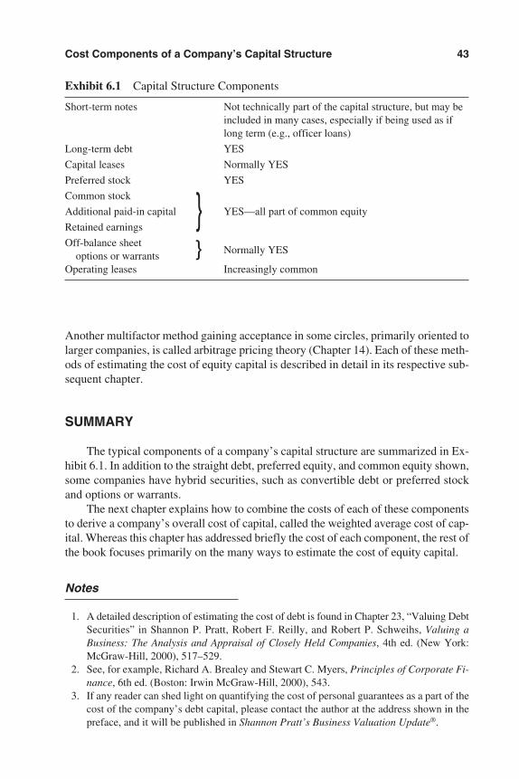
Another multifactor method gaining acceptance in some circles, primarily oriented tolarger companies, is called arbitrage pricing theory (Chapter 14). Each of these meth-ods of estimating the cost of equity capital is described in detail in its respective sub-sequent chapter.
SUMMARY
The typical components of a company’s capital structure are summarized in Ex-hibit 6.1. In addition to the straight debt, preferred equity, and common equity shown,some companies have hybrid securities, such as convertible debt or preferred stockand options or warrants.
The next chapter explains how to combine the costs of each of these componentsto derive a company’s overall cost of capital, called the weighted average cost of cap-ital. Whereas this chapter has addressed briefly the cost of each component, the rest ofthe book focuses primarily on the many ways to estimate the cost of equity capital.
Notes
1. A detailed description of estimating the cost of debt is found in Chapter 23, “Valuing DebtSecurities” in Shannon P. Pratt, Robert F. Reilly, and Robert P. Schweihs, Valuing aBusiness: The Analysis and Appraisal of Closely Held Companies, 4th ed. (New York:McGraw-Hill, 2000), 517–529.
2. See, for example, Richard A. Brealey and Stewart C. Myers, Principles of Corporate Fi-nance, 6th ed. (Boston: Irwin McGraw-Hill, 2000), 543.
3. If any reader can shed light on quantifying the cost of personal guarantees as a part of thecost of the company’s debt capital, please contact the author at the address shown in thepreface, and it will be published in Shannon Pratt’s Business Valuation Update®.
Cost Components of a Company’s Capital Structure 43
Exhibit 6.1 Capital Structure Components
Short-term notes Not technically part of the capital structure, but may beincluded in many cases, especially if being used as iflong term (e.g., officer loans)
Long-term debt YES
Capital leases Normally YES
Preferred stock YES
Common stock
Additional paid-in capital YES—all part of common equity
Retained earnings
Off-balance sheetNormally YESoptions or warrants
Operating leases Increasingly common
}}
3953 P-06 8/29/02 2:21 PM Page 43

4. A detailed description of estimating the cost of preferred stock is found in Chapter 24,“Valuing Preferred Stock,” in Pratt, Reilly, and Schweihs, Valuing a Business, 531–552.
5. Valuing warrants and options is beyond the scope of this book. For an extensive treatmentof this topic, see Chapters 20 to 22 in Brealey and Myers, Principles of Corporate Finance.
44 Cost of Capital Basics
3953 P-06 8/29/02 2:21 PM Page 44
45
Chapter 7
Weighted Average Cost of CapitalWhen to Use Weighted Average Cost of CapitalWeighted Average Cost of Capital FormulaComputing WACC for a Public CompanyComputing WACC for a Private CompanyShould an Actual or a Hypothetical Capital Structure Be Used?Summary
In the last chapter we identified components of a company’s capital structure.Here we blend their costs together to estimate the company’s overall cost of capital.In other words, we want to estimate the weighted cost for all of the company’s investedcapital or the capital to be committed to a specific project.
WHEN TO USE WEIGHTED AVERAGE COST OF CAPITAL
The most obvious instance in which to use weighted average cost of capital(WACC) is when the objective is to value the entire capital structure of a company.An example would be when considering an acquisition and the buyer expects to payoff all equity and debt holders and refinance the whole company in a different waythat better suits the buyer. Sometimes WACC is also used even when the objective isultimately to value only the equity. One would value the entire capital structure andthen subtract the market value of the debt to estimate the value of the equity. Thisprocedure frequently is used in highly leveraged situations.
Weighted average cost of capital is especially appropriate for project selection incapital budgeting. The proportions of debt and equity that could be available to fi-nance various projects might differ according to the project (e.g., asset-intensive pro-jects may be financed with more debt), and the cost of capital should be based on thespecific investment.
This introduces the idea that we have to compute or estimate the weight (per-centage of the total) for each component of the capital structure. The critical point isthat the relative weightings of debt and equity or other capital components are basedon the market values of each component, not on the book values.
3953 P-07 8/29/02 2:21 PM Page 45
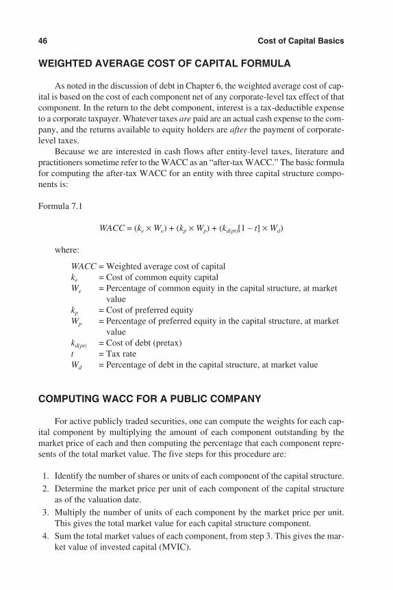
WEIGHTED AVERAGE COST OF CAPITAL FORMULA
As noted in the discussion of debt in Chapter 6, the weighted average cost of cap-ital is based on the cost of each component net of any corporate-level tax effect of thatcomponent. In the return to the debt component, interest is a tax-deductible expenseto a corporate taxpayer. Whatever taxes are paid are an actual cash expense to the com-pany, and the returns available to equity holders are after the payment of corporate-level taxes.
Because we are interested in cash flows after entity-level taxes, literature andpractitioners sometime refer to the WACC as an “after-tax WACC.” The basic formulafor computing the after-tax WACC for an entity with three capital structure compo-nents is:
Formula 7.1
WACC = (ke × We) + (kp × Wp) + (kd(pt)[1 – t] × Wd)
where:
WACC = Weighted average cost of capitalke = Cost of common equity capitalWe = Percentage of common equity in the capital structure, at market
valuekp = Cost of preferred equityWp = Percentage of preferred equity in the capital structure, at market
valuekd(pt) = Cost of debt (pretax)t = Tax rateWd = Percentage of debt in the capital structure, at market value
COMPUTING WACC FOR A PUBLIC COMPANY
For active publicly traded securities, one can compute the weights for each cap-ital component by multiplying the amount of each component outstanding by themarket price of each and then computing the percentage that each component repre-sents of the total market value. The five steps for this procedure are:
1. Identify the number of shares or units of each component of the capital structure.
2. Determine the market price per unit of each component of the capital structureas of the valuation date.
3. Multiply the number of units of each component by the market price per unit.This gives the total market value for each capital structure component.
4. Sum the total market values of each component, from step 3. This gives the mar-ket value of invested capital (MVIC).
46 Cost of Capital Basics
3953 P-07 8/29/02 2:21 PM Page 46
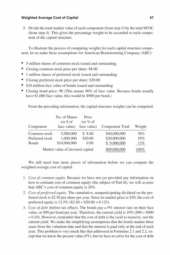
5. Divide the total market value of each component (from step 3) by the total MVIC(from step 4). This gives the percentage weight to be accorded to each compo-nent of the capital structure.
To illustrate the process of computing weights for each capital structure compo-nent, let us make these assumptions for American Brainstorming Company (ABC):
• 5 million shares of common stock issued and outstanding
• Closing common stock price per share: $8.00
• 1 million shares of preferred stock issued and outstanding
• Closing preferred stock price per share: $20.00
• $10 million face value of bonds issued and outstanding
• Closing bond price: 90 (This means 90% of face value. Because bonds usuallyhave $1,000 face value, this would be $900 per bond.)
From the preceding information, the capital structure weights can be computed:
No. of Shares Price(or $ of (or % of
Component face value) face value) Component Total Weight
Common stock 5,000,000 $ 8.00 $40,000,000 58%Preferred stock 1,000,000 $20.00 $20,000,000 29%Bonds $10,000,000 0.90 $ 9,000,000 13%————— ——–
Market value of invested capital $69,000,000 100%————— —–—————— —–—
We still need four more pieces of information before we can compute theweighted average cost of capital:
1. Cost of common equity. Because we have not yet provided any information onhow to estimate cost of common equity (the subject of Part II), we will assumethat ABC’s cost of common equity is 20%.
2. Cost of preferred equity. The cumulative, nonparticipating dividend on the pre-ferred stock is $2.50 per share per year. Since its market price is $20, the cost ofpreferred equity is 12.5% ($2.50 ÷ $20.00 = 0.125).
3. Cost of debt (before tax effect). The bonds pay a 9% interest rate on their facevalue, or $90 per bond per year. Therefore, the current yield is 10% ($90 ÷ $900= 0.10). However, remember that the cost of debt is the yield to maturity, not thecurrent yield. We make the simplifying assumptions that the bonds mature threeyears from the valuation date and that the interest is paid only at the end of eachyear. This problem is very much like that addressed in Formulas 2.1 and 2.2, ex-cept that we know the present value (PV), but we have to solve for the cost of debt
Weighted Average Cost of Capital 47
3953 P-07 8/29/02 2:21 PM Page 47
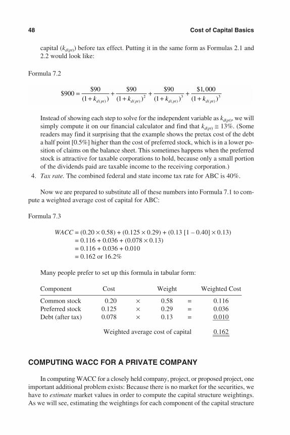
capital (kd(pt)) before tax effect. Putting it in the same form as Formulas 2.1 and2.2 would look like:
Formula 7.2
Instead of showing each step to solve for the independent variable as kd(pt), we willsimply compute it on our financial calculator and find that kd(pt) ≅ 13%. (Somereaders may find it surprising that the example shows the pretax cost of the debta half point [0.5%] higher than the cost of preferred stock, which is in a lower po-sition of claims on the balance sheet. This sometimes happens when the preferredstock is attractive for taxable corporations to hold, because only a small portionof the dividends paid are taxable income to the receiving corporation.)
4. Tax rate. The combined federal and state income tax rate for ABC is 40%.
Now we are prepared to substitute all of these numbers into Formula 7.1 to com-pute a weighted average cost of capital for ABC:
Formula 7.3
WACC = (0.20 × 0.58) + (0.125 × 0.29) + (0.13 [1 – 0.40] × 0.13)= 0.116 + 0.036 + (0.078 × 0.13)= 0.116 + 0.036 + 0.010= 0.162 or 16.2%
Many people prefer to set up this formula in tabular form:
Component Cost Weight Weighted Cost
Common stock 0.20 × 0.58 = 0.116Preferred stock 0.125 × 0.29 = 0.036Debt (after tax) 0.078 × 0.13 = 0.010——–
Weighted average cost of capital 0.162——––––––
COMPUTING WACC FOR A PRIVATE COMPANY
In computing WACC for a closely held company, project, or proposed project, oneimportant additional problem exists: Because there is no market for the securities, wehave to estimate market values in order to compute the capital structure weightings.As we will see, estimating the weightings for each component of the capital structure
$$
( )
$
( )
$
( )
$ ,
( )( ) ( ) ( ) ( )
90090
1
90
1
90
1
1 000
12 3 3=+
++
++
++k k k kd pt d pt d pt d pt
48 Cost of Capital Basics
3953 P-07 8/29/02 2:21 PM Page 48
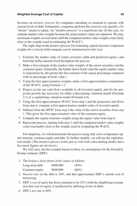
becomes an iterative process for companies intending or assumed to operate withcurrent levels of debt. Fortunately, computers perform this exercise very quickly. (To“iterate” means to repeat. An “iterative process” is a repetitious one. In this case, weestimate market value weights because the actual market values are unknown. We mayreestimate weights several times until the computed market value weights come fairlyclose to the weights used in estimating the WACC.)
The eight steps in the iterative process for estimating capital structure componentweights for a closely held company can be summarized in this way:
1. Estimate the market value of senior securities (debt and preferred equity), andhold that dollar amount fixed throughout the process.
2. Make a first estimate of the market value weights of the senior securities and thecommon equity. (Generally, the farther above book value the equity market valueis expected to be, the greater the first estimate of the equity percentage comparedwith its percentage at book value.)
3. Using the first approximation weights, make a first approximation computationof the WACC, using Formula 7.1.
4. Project (a) the net cash flows available to all invested capital, and (b) the pro-jected growth rate necessary for either a discounting valuation model (Formula2.1) or a capitalizing valuation model (Formula 4.4).
5. Using the first approximation WACC from step 3 and the projected cash flowsfrom step 4, compute a first approximation market value of invested capital.
6. Subtract from the MVIC from step 4 the value of the senior securities from step1. This gives the first approximation value of the common equity.
7. Compute the capital structure weights using the equity value from step 6.
8. Repeat the process, starting with step 3, until the computed market value weightscome reasonably close to the weights used in computing the WACC.
For simplicity, we will demonstrate this process using only a two-component cap-ital structure, common equity and debt. To further simplify, we will use the capitaliza-tion model. (The iterative process works just as well with a discounting model, but afew more figures are involved.)
We will carry out the example based on these six assumptions for the Donald E.Frump company (DEF):
1. The balance sheet shows book values as follows:
Long-term debt $400,000 (40%)
Common equity $600,000 (60%)
2. Interest rate on the debt is 10%, and that approximates DEF’s current cost ofborrowing.
3. DEF’s cost of equity has been estimated to be 25% (with the simplifying assump-tion that cost of equity is unaffected by differing levels of debt).
4. DEF’s tax rate is 40%.
Weighted Average Cost of Capital 49
3953 P-07 8/29/02 2:21 PM Page 49
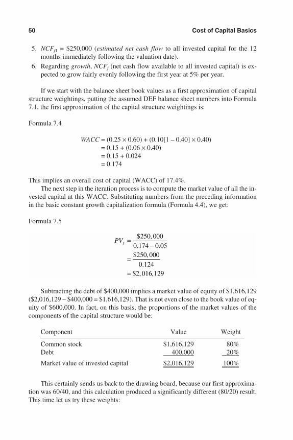
5. NCFf1 = $250,000 (estimated net cash flow to all invested capital for the 12months immediately following the valuation date).
6. Regarding growth, NCFf (net cash flow available to all invested capital) is ex-pected to grow fairly evenly following the first year at 5% per year.
If we start with the balance sheet book values as a first approximation of capitalstructure weightings, putting the assumed DEF balance sheet numbers into Formula7.1, the first approximation of the capital structure weightings is:
Formula 7.4
WACC = (0.25 × 0.60) + (0.10[1 – 0.40] × 0.40)= 0.15 + (0.06 × 0.40)= 0.15 + 0.024= 0.174
This implies an overall cost of capital (WACC) of 17.4%.The next step in the iteration process is to compute the market value of all the in-
vested capital at this WACC. Substituting numbers from the preceding informationin the basic constant growth capitalization formula (Formula 4.4), we get:
Formula 7.5
Subtracting the debt of $400,000 implies a market value of equity of $1,616,129($2,016,129 – $400,000 = $1,616,129). That is not even close to the book value of eq-uity of $600,000. In fact, on this basis, the proportions of the market values of thecomponents of the capital structure would be:
Component Value Weight
Common stock $1,616,129 80%Debt 400,000 20%————– ——–Market value of invested capital $2,016,129 100%————– ——–————– ——–
This certainly sends us back to the drawing board, because our first approxima-tion was 60/40, and this calculation produced a significantly different (80/20) result.This time let us try these weights:
PVf =−
=
=
$ ,
. .$ ,
.$ , ,
250 000
0 174 0 05250 000
0 1242 016 129
50 Cost of Capital Basics
3953 P-07 8/29/02 2:21 PM Page 50
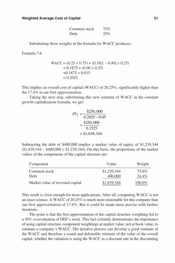
Common stock 75%Debt 25%
Substituting these weights in the formula for WACC produces:
Formula 7.6
WACC = (0.25 × 0.75) + (0.10[1 – 0.40] × 0.25)= 0.1875 + (0.06 × 0.25)=0.1875 + 0.015= 0.2025
This implies an overall cost of capital (WACC) of 20.25%, significantly higher thanthe 17.4% in our first approximation.
Taking the next step, substituting this new estimate of WACC in the constantgrowth capitalization formula, we get:
Subtracting the debt of $400,000 implies a market value of equity of $1,239,344($1,639,344 – $400,000 = $1,239,344). On this basis, the proportions of the marketvalues of the components of the capital structure are:
Component Value Weight
Common stock $1,239,344 75.6%Debt 400,000 24.4%————– –——–Market value of invested capital $1,639,344 100.0%————– –——–————– –——–
This result is close enough for most applications. After all, computing WACC is notan exact science. A WACC of 20.25% is much more reasonable for this company thanour first approximation of 17.4%. But it could be made more precise with furtheriterations.
The point is that the first approximation of the capital structure weighting led toa 30% overvaluation of DEF’s stock. This fact certainly demonstrates the importanceof using capital structure component weightings at market value, not at book value, toestimate a company’s WACC. The iterative process can develop a good estimate ofthe WACC and therefore a sound and defensible estimate of the value of the overallcapital, whether the valuation is using the WACC as a discount rate in the discounting
PVf =−
=
=
$ ,
. .$ ,
.$ , ,
250 000
0 2025 0 05250 000
0 15251 639 344
Weighted Average Cost of Capital 51
3953 P-07 8/29/02 2:21 PM Page 51
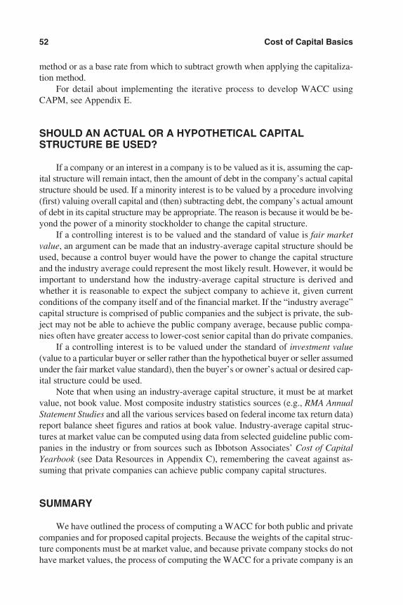
method or as a base rate from which to subtract growth when applying the capitaliza-tion method.
For detail about implementing the iterative process to develop WACC usingCAPM, see Appendix E.
SHOULD AN ACTUAL OR A HYPOTHETICAL CAPITALSTRUCTURE BE USED?
If a company or an interest in a company is to be valued as it is, assuming the cap-ital structure will remain intact, then the amount of debt in the company’s actual capitalstructure should be used. If a minority interest is to be valued by a procedure involving(first) valuing overall capital and (then) subtracting debt, the company’s actual amountof debt in its capital structure may be appropriate. The reason is because it would be be-yond the power of a minority stockholder to change the capital structure.
If a controlling interest is to be valued and the standard of value is fair marketvalue, an argument can be made that an industry-average capital structure should beused, because a control buyer would have the power to change the capital structureand the industry average could represent the most likely result. However, it would beimportant to understand how the industry-average capital structure is derived andwhether it is reasonable to expect the subject company to achieve it, given currentconditions of the company itself and of the financial market. If the “industry average”capital structure is comprised of public companies and the subject is private, the sub-ject may not be able to achieve the public company average, because public compa-nies often have greater access to lower-cost senior capital than do private companies.
If a controlling interest is to be valued under the standard of investment value(value to a particular buyer or seller rather than the hypothetical buyer or seller assumedunder the fair market value standard), then the buyer’s or owner’s actual or desired cap-ital structure could be used.
Note that when using an industry-average capital structure, it must be at marketvalue, not book value. Most composite industry statistics sources (e.g., RMA AnnualStatement Studies and all the various services based on federal income tax return data)report balance sheet figures and ratios at book value. Industry-average capital struc-tures at market value can be computed using data from selected guideline public com-panies in the industry or from sources such as Ibbotson Associates’ Cost of CapitalYearbook (see Data Resources in Appendix C), remembering the caveat against as-suming that private companies can achieve public company capital structures.
SUMMARY
We have outlined the process of computing a WACC for both public and privatecompanies and for proposed capital projects. Because the weights of the capital struc-ture components must be at market value, and because private company stocks do nothave market values, the process of computing the WACC for a private company is an
52 Cost of Capital Basics
3953 P-07 8/29/02 2:21 PM Page 52
iterative one, starting with approximations of market value weights of capital struc-ture components.
Under some circumstances (e.g., a minority interest valuation), a company’s ac-tual (currently existing) capital structure may be used to estimate the WACC. If acontrolling interest valuation is sought where it is reasonable to alter the company’scapital structure, a hypothetical capital structure may be used to estimate the WACC.
There is much controversy about the potential impact that altering the capitalstructure has on the WACC.
Weighted Average Cost of Capital 53
3953 P-07 8/29/02 2:21 PM Page 53

3953 P-07 8/29/02 2:21 PM Page 54
PART II
Estimating the Cost ofEquity Capital
3953 P-08 8/29/02 2:21 PM Page 55

3953 P-08 8/29/02 2:21 PM Page 56
57
Chapter 8
Build-up ModelsFormula for the Equity Cost of Capital Build-up ModelRisk-free Rate
Risk-free Rate Represented by U.S. Treasury SecuritiesComponents of the Risk-free RateWhy Only Three Specific Maturities?Selecting the Best Risk-free Maturity
Equity Risk PremiumIbbotson Associates Is the Primary Source of Historical Risk Premium DataArithmetic or Geometric Mean Historical Average Equity Risk Premium?Over What Historical Time Period Should the Equity Risk Premium Be
Calculated?Estimating Equity Risk Premia by the DCF Method
Small Stock PremiumCompany-specific Risk Premium
Size Smaller Than the Smallest Size Premium GroupIndustry RiskVolatility of ReturnsLeverageOther Company-specific Factors
Example of a Build-up Model
Summary
Previous chapters discussed the cost of capital in terms of its two major compo-nents, a risk-free rate and a risk premium. This chapter examines these componentsin general, dividing the equity risk premium into its three principal subcomponents.
Accordingly, the typical “build-up model” for estimating the cost of common eq-uity capital consists of two components:
1. A “risk-free” rate
2. A premium for risk, including any or all of the following subcomponents:
a. A general equity risk premium
b. A size premium
c. A company-specific risk premium
In international investing, there may also be a country-specific risk premium, reflect-ing uncertainties owing to economic and political instability in the particular country.
3953 P-08 8/29/02 2:21 PM Page 57
With respect to using the weighted average cost of capital (WACC) in other countries,one should consider the risk-free rate in the foreign country (e.g., interest rate on thatcountry’s government debt) and the risk premium in that country as measured by stockmarket returns in excess of return on the foreign government bonds. The risk-free rateand foreign equity risk premium are likely to incorporate the foreign country-specificrisk premium, including any currency-related risk. In some countries there might bea risk discount compared with the United States.
It is probably a mistake to use the U.S. risk-free rate in determining foreign coun-try cost of capital. If a foreign country-specific risk premium is not available, whichoften is the case, especially with smaller countries, one can use the U.S. risk premiumapplied to the foreign risk-free rate. (Bloomberg is an excellent source of foreigncountry government bond rates.) Other adjustments may be necessary to account forregulatory or other economic differences.
FORMULA FOR THE EQUITY COST OF CAPITAL BUILD-UP MODEL
Stating the preceding concept in a formula, the equity cost of capital build-upmodel is:
Formula 8.1
E(Ri) = Rf + RPm + RPs + RPu
where:
E(Ri) = Expected (market required) rate of return on security iRf = Rate of return available on a risk-free security as of the valuation
dateRPm = General equity risk premium for the “market”RPs = Risk premium for small sizeRPu = Risk premium attributable to the specific company or to the
industry (the u stands for unsystematic risk, as defined in Chapter 5)
After discussing how to develop each of these four components, we will substitutesome numbers into the formula to reach an estimated cost of equity capital for a sam-ple company.
An additional possible component, industry risk, is discussed in a later section inthis chapter.
RISK-FREE RATE
The general notion of a “risk-free rate” is the return available as of the valuationdate on a security that the market generally regards as free of the risk of default.
58 Estimating the Cost of Equity Capital
3953 P-08 8/29/02 2:21 PM Page 58
Risk-free Rate Represented by U.S. Treasury Securities
In the build-up model (as well as in other models), analysts typically use the yieldto maturity on U.S. government securities, as of the effective valuation date, as the risk-free rate. They generally choose U.S. Treasury obligations of one of the followingmaturities:
• 30 days
• 5 years
• 20 years
Sources for yields to maturity for maturities of any length as of any valuation date canbe found in the daily financial press. (It usually is not possible to find yields to matchthe exact length of maturity. One should just choose the closest maturity available.)
Components of the Risk-free Rate
The so-called risk-free rate reflects three components:
1. Rental rate: A real return for lending the funds over the investment period, thusforgoing consumption for which the funds otherwise could be used
2. Inflation: The expected rate of inflation over the term of the risk-free investment
3. Maturity risk or investment rate risk: As discussed in Chapter 5, the risk that theprincipal’s market value will rise or fall during the period to maturity as a func-tion of changes in the general level of interest rates
All three of these economic factors are embedded in the yield to maturity for anygiven maturity length. However, it is not possible to observe the market consensusabout how much of the yield for any given maturity is attributable to each of thesefactors.
Very importantly, note that this basic risk-free rate includes inflation. Therefore,when this rate is used to estimate a cost of capital to discount expected future cashflows, those future cash flows also should reflect the effect of inflation. In the eco-nomic sense of nominal versus real dollars, we are building a cost of capital in nom-inal terms, and it should be used to discount expected returns that also are expressedin nominal terms.
Why Only Three Specific Maturities?
The risk-free rate typically is chosen from one of only three specific maturitiesbecause the build-up model incorporates a general equity risk premium often basedon historical data developed by Ibbotson Associates.
Build-up Models 59
3953 P-08 8/29/02 2:21 PM Page 59
• Ibbotson data provide short-term, intermediate-term, and long-term equity risk pre-mium series, based on data corresponding to the aforementioned three maturities.
• Twenty years is the longest maturity because the Ibbotson data go all the way backto 1926, and 20 years was the longest U.S. Treasury obligation issued during theearlier years of that time period.
Selecting the Best Risk-free Maturity
The consensus of financial analysts today is to use the 20-year U.S. Treasuryyield to maturity as of the effective date of valuation because:
• It most closely matches the often-assumed perpetual lifetime horizon of an equityinvestment.
• The longest-term yields to maturity fluctuate considerably less than short-termrates and thus are less likely to introduce unwarranted short-term distortions intothe actual cost of capital.
• People generally are willing to recognize and accept that the maturity risk is em-bedded in this base, or otherwise risk-free, rate.
• It matches the longest-term bond over which the equity risk premium is measuredin the Ibbotson Associates data series.
Many analysts use a 30-year yield, but as a practical matter it usually does notdiffer greatly from the 20-year yield.
Sometimes analysts select a five-year rate to match the perceived investmenthorizon for the subject equity investment. The 30-day rate is the purest risk-free baserate because it contains virtually no maturity risk. If inflation is high, it does reflect theinflation component, but it contains little compensation for inflation uncertainty.
To obtain a 20-year yield, most analysts go to the financial press (e.g., The WallStreet Journal, The New York Times) as of the valuation date and find the yield on abond originally issued for 30 years with approximately 20 years left to maturity. TheSt. Louis branch of the Federal Reserve Bank also tracks 20-year yields. The directlink to its Web site is: http://www.stls.frg.org/fred/data/irates/gs20.
EQUITY RISK PREMIUM
On an equity investment, the return on investment that the investor will (or hasthe opportunity to) realize usually has two components:
1. Distributions during the holding period (e.g., dividends or withdrawals)
2. The capital gain or loss in the value of the investment (For an active public se-curity, it is considered part of the return whether or not the investor chooses torealize it, because the investor has that choice at any time.)
60 Estimating the Cost of Equity Capital
3953 P-08 8/29/02 2:21 PM Page 60
Obviously, these expected amounts of returns on equities are much less certain (ormore risky) than the interest and maturity payments on U.S. Treasury obligations.This difference in riskiness is well documented by much higher standard deviations(year-to-year volatility) in returns on the stock market, compared with the standarddeviation of year-to-year returns on U.S. Treasury obligations.
To accept this greater risk, investors demand higher expected returns for invest-ing in equities than for investing in U.S. Treasury obligations. This differential in ex-pected return on the broad stock market over U.S. Treasury obligations (sometimesreferred to as the excess return, but not to be confused with the excess earnings method)is called the equity risk premium.
In practice, a common method of estimating this expected equity risk premiumis to use historical data. It is common to compute it as the average excess return(broad stock market over U.S. Treasuries) over some historical period of time. Be-cause cost of capital is a forward-looking concept, a key implied assumption whenusing historical data is that the amount of excess return that investors expect for in-vesting in stocks (over the amount expected from Treasuries) for their future timehorizon is approximately equal to the excess returns that have actually been achievedin the broad stock market in the historical period for which the equity risk premiumwas computed.
Ibbotson now calculates the arithmetic average equity risk premium on two mea-sures of the broad market:
1. Standard & Poor’s (S&P) 500 Index
2. New York Stock Exchange (NYSE) Composite Index
In the 2002 SBBI Valuation Edition, these equity risk premia were 7.4% and 7.1%,respectively. The 2002 Valuation Edition says nothing about which is better to useunder what circumstances. In the following examples, we will use the S&P 500, be-cause that is what Ibbotson uses in most of its examples.
Ibbotson Associates Is the Primary Source of Historical RiskPremium Data
Ibbotson Associates publishes historical risk premium data in its annually updatedStocks, Bonds, Bills and Inflation (SBBI), Classic Edition and Valuation Edition. Thesepublications are described in some detail in Chapter 13 on using Ibbotson data, andordering information is included in Appendix C. These sources are a core part of anycorporate finance data library, especially for a practitioner of business valuations.
Arithmetic or Geometric Mean Historical Average Equity Risk Premium?
Ibbotson publishes both an arithmetic and a geometric mean equity risk premiumseries. In the arithmetic mean series, the procedure is to add up all the excess returnsover the periods and divide by the number of periods.
Build-up Models 61
3953 P-08 8/29/02 2:21 PM Page 61
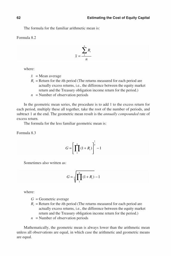
The formula for the familiar arithmetic mean is:
Formula 8.2
where:
x̄ = Mean averageRi = Return for the ith period (The returns measured for each period are
actually excess returns, i.e., the difference between the equity marketreturn and the Treasury obligation income return for the period.)
n = Number of observation periods
In the geometric mean series, the procedure is to add 1 to the excess return foreach period, multiply these all together, take the root of the number of periods, andsubtract 1 at the end. The geometric mean result is the annually compounded rate ofexcess return.
The formula for the less familiar geometric mean is:
Formula 8.3
Sometimes also written as:
where:
G = Geometric averageRi = Return for the ith period (The returns measured for each period are
actually excess returns, i.e., the difference between the equity marketreturn and the Treasury obligation income return for the period.)
n = Number of observation periods
Mathematically, the geometric mean is always lower than the arithmetic meanunless all observations are equal, in which case the arithmetic and geometric meansare equal.
G Ri
n
n= + −∏ ( )1 11
G Ri
n n
= +
−∏ ( )1 11
1
x
R
n
i
n
=∑
1
62 Estimating the Cost of Equity Capital
3953 P-08 8/29/02 2:21 PM Page 62
Ibbotson’s position is that, for valuation purposes, the historical equity risk pre-mium should be the arithmetic mean applied to the expected value of the probabilitydistribution of the expected return for each period. This is discussed further in Chap-ter 13 on using Ibbotson data.
The Ibbotson position that the long-term arithmetic average equity risk premiumis the best proxy for today’s equity risk premium is widely accepted. For example, thisview is supported by one of the leading corporate finance texts, Brealey and Myers’Principles of Corporate Finance, where the authors state, “If the cost of capital is esti-mated from historic returns or risk premiums, use arithmetic averages, not compoundrates of return.”1 However, this view is not universally held. For a contrary view (i.e.,that the true market risk premium lies somewhere between the arithmetic and geo-metric averages), see Tom Copeland, Tim Koller, and Jack Murrin’s Valuation: Mea-suring and Managing the Value of Companies.2 There have also been articles on thiscontroversy in Business Valuation Review, the quarterly journal of the Business Val-uation Committee of the American Society of Appraisers.3 The arithmetic mean istechnically correct when applied to the expected value of the cash flows. However,because a long time period is needed to develop a statistically valid historical risk pre-mium, a short historical period could produce a high or low indicated cost of capitalrelative to any specific date’s current market conditions.
Over What Historical Time Period Should the Equity RiskPremium Be Calculated?
Regarding the historical time period over which equity risk should be calculated,Ibbotson offers two observations:
1. Reasons to focus on recent history:
a. The recent past may be most relevant to an investor.
b. Return patterns may change over time.
c. The longer period includes “major events” (e.g., World War I, World War II,the Depression) that have not repeated in some time.
2. Reasons to focus on long-term history:
a. Long-term historical returns have shown surprising stability.
b. Short-term observations may lead to illogical forecasts.
c. Focusing on the recent past ignores dramatic historical events and their im-pact on market returns. We do not know what major events lie ahead.
d. Law of large numbers: More observations lead to a more accurate estimate.
Exhibit 8.1 shows the arithmetic average equity risk premiums over various timeperiods as calculated by Ibbotson.
Note that as the length of the measurement period shortens, the standard error ofthe estimate widens substantially. This is one reason why Ibbotson advocates usingthe full historical period covered by the data, 1926 through the present, as discussedmore fully in Chapter 13.
Build-up Models 63
3953 P-08 8/29/02 2:21 PM Page 63
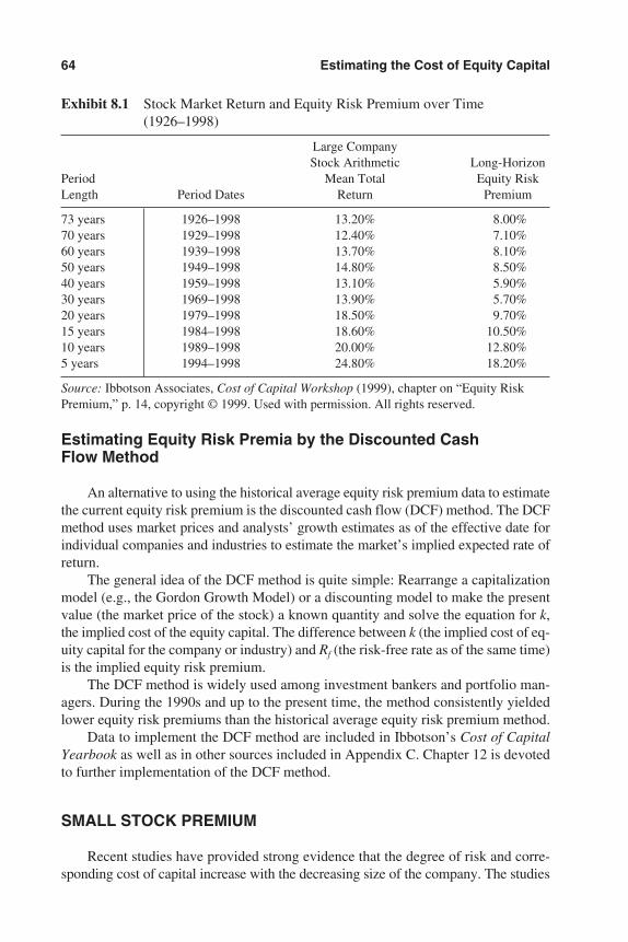
Estimating Equity Risk Premia by the Discounted Cash Flow Method
An alternative to using the historical average equity risk premium data to estimatethe current equity risk premium is the discounted cash flow (DCF) method. The DCFmethod uses market prices and analysts’ growth estimates as of the effective date forindividual companies and industries to estimate the market’s implied expected rate ofreturn.
The general idea of the DCF method is quite simple: Rearrange a capitalizationmodel (e.g., the Gordon Growth Model) or a discounting model to make the presentvalue (the market price of the stock) a known quantity and solve the equation for k,the implied cost of the equity capital. The difference between k (the implied cost of eq-uity capital for the company or industry) and Rf (the risk-free rate as of the same time)is the implied equity risk premium.
The DCF method is widely used among investment bankers and portfolio man-agers. During the 1990s and up to the present time, the method consistently yieldedlower equity risk premiums than the historical average equity risk premium method.
Data to implement the DCF method are included in Ibbotson’s Cost of CapitalYearbook as well as in other sources included in Appendix C. Chapter 12 is devotedto further implementation of the DCF method.
SMALL STOCK PREMIUM
Recent studies have provided strong evidence that the degree of risk and corre-sponding cost of capital increase with the decreasing size of the company. The studies
64 Estimating the Cost of Equity Capital
Exhibit 8.1 Stock Market Return and Equity Risk Premium over Time(1926–1998)
Large CompanyStock Arithmetic Long-Horizon
Period Mean Total Equity RiskLength Period Dates Return Premium
73 years 1926–1998 13.20% 8.00%70 years 1929–1998 12.40% 7.10%60 years 1939–1998 13.70% 8.10%50 years 1949–1998 14.80% 8.50%40 years 1959–1998 13.10% 5.90%30 years 1969–1998 13.90% 5.70%20 years 1979–1998 18.50% 9.70%15 years 1984–1998 18.60% 10.50%10 years 1989–1998 20.00% 12.80%5 years 1994–1998 24.80% 18.20%
Source: Ibbotson Associates, Cost of Capital Workshop (1999), chapter on “Equity RiskPremium,” p. 14, copyright © 1999. Used with permission. All rights reserved.
3953 P-08 8/29/02 2:21 PM Page 64
show that this addition to the equity risk premium is over and above the amount thatwould be warranted solely for the companies’ systematic risk. The next two chaptersexplain the Capital Asset Pricing Model (CAPM) and the proper use of beta. Chap-ter 11 discusses the results of research on this phenomenon as well as the sources.
COMPANY-SPECIFIC RISK PREMIUM
To the extent that the subject company’s risk characteristics are greater or lessthan the typical risk characteristics of the companies from which the equity risk pre-mium and the size premium were drawn, a further adjustment may be necessary to es-timate the cost of capital for the specific company. Such adjustment may be based on(but not necessarily limited to) analysis of five factors:
1. Size smaller than the smallest size premium group
2. Industry risk
3. Volatility of returns
4. Leverage
5. Other company-specific factors
Size Smaller Than the Smallest Size Premium Group
As will be seen in Exhibit 11.4, the smallest size group for which we have spe-cific size premium data averages $30 million in market value of equity, $37 millionin sales, and so forth. If the subject company is somewhat smaller than this cutoff,most observers believe that a further size premium adjustment is warranted, but therehave not yet been adequate empirical studies to quantify this amount. Accordingly, aconservative approach may be appropriate, perhaps adding a point or two to the dis-count rate for a significantly smaller company and leaving any greater adjustments tobe attributed to other specifically identifiable risk factors.
In the first edition of this book, I said that I planned to research this issue usingthe Pratt’s Stats™ private company transaction database. The study is reported inChapter 11 on the size effect. Indeed, the results show that the cost of capital is muchgreater for smaller companies.
Industry Risk
The industry in which the company operates may have more or less risk than theaverage of other companies in the same size category. This differential is very hard toquantify in the build-up model. However, if the company is obviously in a very low-riskindustry (e.g., water distribution) or a very high-risk industry (e.g., airlines), a point ortwo adjustment, either downward or upward, for this factor may be warranted.
Ibbotson Associates now publishes industry risk adjustment factors (see Chapter13), but the industry definitions are quite broad. We understand that the definitions
Build-up Models 65
3953 P-08 8/29/02 2:21 PM Page 65
will continue to grow and be refined down to more discrete Standard Industrial Clas-sification (SIC) sorts than what we see so far.4 It is too early to tell how well they willstand up to testing in the market.
As noted earlier, Ibbotson’s SBBI Valuation Edition 2002 Yearbook presents anexpanded alternative build-up model that includes a separate variable for the indus-try risk premium. This model is shown in Formula 8.4:
Formula 8.4
E(Ri) = Rf + RPm + RPs +/– RP□+ Rpu
where:
E(Ri) = Expected rate of returnRf = Risk-free rate of returnRPm = Equity risk premium (market risk)RPs = Size premiumRPi = Industry risk premiumRPu = Company-specific risk premium (unsystematic risk)
Volatility of Returns
High volatility of returns (usually measured by the standard deviation of historicalreturns over some period) is another risk factor. However, without comparable data forthe average of the other companies in the size category and/or industry, it is not possi-ble to make a quantified comparison. If the analyst perceives that the subject companyreturns are either unusually stable or unusually volatile compared with others in the sizecategory and/or industry, some adjustment for this factor may be warranted.
Leverage
Leverage is clearly a factor that can be compared between the subject companyand its size peers. Exhibit 11.4 gives both the market value of equity and the marketvalue of invested capital for each size category.
For example, the smallest size category averages $30 million in market value ofequity and $41 million in market value of invested capital, or a capital structure ofroughly 25% debt and 75% equity, at market value. Size breakdowns of other sizemeasures show generally similar capital structures. If the subject company’s capitalstructure significantly departs from this average, some upward or downward adjust-ment to the cost of equity relative to the average company in the size category wouldseem warranted. For example, highly leveraged companies should have higher equitycosts of capital compared with companies with lower debt levels, all else being equal.Of course, a decrease in the required equity return might be warranted if the subject’scapital structure has little or no debt.
66 Estimating the Cost of Equity Capital
3953 P-08 8/29/02 2:21 PM Page 66
Other Company-specific Factors
Other factors specific to a particular company that affect risk could include, forexample:
• Concentration of customer base
• Key person dependence
• Key supplier dependence
• Abnormal present or pending competition
• Pending regulatory changes
• Pending lawsuits
• A wide variety of other possible specific factors
Because the size premium tends to reflect some factors of this type, the analyst shouldadjust further only for specific items that are truly unique to the subject company.Unfortunately, despite the widespread use by analysts and appraisers of a company-specific risk premium in a build-up (or CAPM) model, I am not aware of any acade-mic research on the subject, and it remains in the realm of the analyst’s judgment.
EXAMPLE OF A BUILD-UP MODEL
Now that we have discussed the factors in the build-up model, we can substitutesome numbers into Formula 8.1. We start with the following four assumptions aboutShannon’s Bull Market (SBM), a regional steakhouse chain with excellent food andfriendly service:
1. Risk-free rate. We will use the 20-year Treasury bond, for which the yield to ma-turity at the valuation date was 6.5%.
2. Equity risk premium. We will use the Ibbotson Associates’ arithmetic averageequity risk premium. The SBBI Valuation Edition 2002 Yearbook shows that tobe 7.4%.
3. Size premium. The SBBI Valuation Edition 2002 Yearbook shows that the sizepremium for the tenth decile—smallest 10% of New York Stock Exchange(NYSE) stocks with American Stock Exchange (AMEX) and Nasdaq StockMarket (Nasdaq) stocks included—over and above the return estimated byCAPM is 5.33%.5
4. Company-specific risk premium. SBM is considerably smaller than the average ofthe smallest 10% of NYSE stocks, and our analyst perceives that the restaurantindustry is riskier than the average for those companies. Although the assessmentis somewhat subjective, our analyst recommends adding a company-specific riskfactor of 3.0% because of risk factors identified as unique to this company.
5. Possibly, an industry adjustment factor.
Build-up Models 67
3953 P-08 8/29/02 2:21 PM Page 67
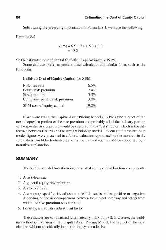
Substituting the preceding information in Formula 8.1, we have the following:
Formula 8.5
E(Ri) = 6.5 + 7.4 + 5.3 + 3.0= 19.2
So the estimated cost of capital for SBM is approximately 19.2%.Some analysts prefer to present these calculations in tabular form, such as the
following:
Build-up Cost of Equity Capital for SBM
Risk-free rate 6.5%Equity risk premium 7.4%Size premium 5.3%Company-specific risk premium 3.0%——–SBM cost of equity capital 19.2%——–——–
If we were using the Capital Asset Pricing Model (CAPM) (the subject of thenext chapter), a portion of the size premium and probably all of the industry portionof the specific risk premium would be captured in the “beta” factor, which is the dif-ference between CAPM and the straight build-up model. Of course, if these build-upmodel figures were presented in a formal valuation report, each of the numbers in thecalculation would be footnoted as to its source, and each would be supported by anarrative explanation.
SUMMARY
The build-up model for estimating the cost of equity capital has four components:
1. A risk-free rate
2. A general equity risk premium
3. A size premium
4. A company-specific risk adjustment (which can be either positive or negative,depending on the risk comparisons between the subject company and others fromwhich the size premium was derived)
5. Possibly, an industry adjustment factor
These factors are summarized schematically in Exhibit 8.2. In a sense, the build-up method is a version of the Capital Asset Pricing Model, the subject of the nextchapter, without specifically incorporating systematic risk.
68 Estimating the Cost of Equity Capital
3953 P-08 8/29/02 2:21 PM Page 68
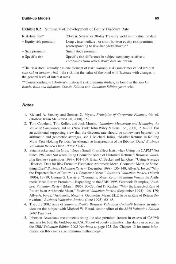
Notes
1. Richard A. Brealey and Stewart C. Myers, Principles of Corporate Finance, 6th ed.(Boston: Irwin McGraw-Hill, 2000), 157.
2. Tom Copeland, Tim Koller, and Jack Murrin, Valuation: Measuring and Managing theValue of Companies, 3rd ed. (New York: John Wiley & Sons, Inc., 2000), 218–221. Foran additional supporting view that the discount rate should be somewhere between thearithmetic and geometric averages, see J. Michael Julius, “Market Returns in RollingMulti-Year Holding Periods: An Alternative Interpretation of the Ibbotson Data,” BusinessValuation Review (June 1996): 57–63.
3. Brian Becker and Ian Gray, “Does a Small Firm Effect Exist when Using the CAPM? NotSince 1980 and Not when Using Geometric Mean of Historical Returns,” Business Valua-tion Review (September 1999): 104–107; Brian C. Becker and Ian Gray, “Using AverageHistorical Data for Risk Premium Estimates: Arithmetic Mean, Geometric Mean, or Some-thing Else?” Business Valuation Review (December 1998): 136–140; Allyn A. Joyce, “Whythe Expected Rate of Return is a Geometric Mean,” Business Valuation Review (March1996): 17–19; George G. Cassiere, “Geometric Mean Return Premium Versus the Arith-metic Mean Return Premium—Expanding on the SBBI 1995 Yearbook Examples,” Busi-ness Valuation Review (March 1996): 20–23; Paul D. Kaplan, “Why the Expected Rate ofReturn is an Arithmetic Mean,” Business Valuation Review (September 1995): 126–129;Allyn A. Joyce, “Arithmetic Mean vs. Geometric Mean: THE Issue in Rate of Return De-rivation,” Business Valuation Review (June 1995): 62–68.
4. The July 2002 issue of Shannon Pratt’s Business Valuation Update® features an inter-view on this subject with Michael W. Barad, senior editor of the SBBI Valuation Edition2002 Yearbook.
5. Ibbotson Associates recommends using the size premium (return in excess of CAPM)analysis for both the build-up and CAPM cost of equity estimates. This data can be seen inthe SBBI Valuation Edition 2002 Yearbook at page 125. See Chapter 13 for more infor-mation on Ibbotson’s size premium methodology.
Build-up Models 69
Exhibit 8.2 Summary of Development of Equity Discount Rate
Risk-free rate* 20-year, 5-year, or 30-day Treasury yield as of valuation date
+ Equity risk premium Long-, intermediate-, or short-horizon equity risk premium(corresponding to risk-free yield above)**
+ Size premium Small stock premium
± Specific risk Specific risk difference in subject company relative tocompanies from which above data are drawn
*The “risk-free” actually has one element of risk: maturity risk (sometimes called interestrate risk or horizon risk)—the risk that the value of the bond will fluctuate with changes inthe general level of interest rates.
**Corresponding to Ibbotson’s historical risk premium studies, as found in the Stocks,Bonds, Bills and Inflation, Classic Edition and Valuation Edition yearbooks.
3953 P-08 8/29/02 2:21 PM Page 69
70
Chapter 9
Capital Asset Pricing Model1
Concept of Systematic RiskBackground of the Capital Asset Pricing ModelSystematic and Unsystematic RiskUsing Beta to Estimate Expected Rate of ReturnExpanding CAPM to Incorporate Size Premium and Specific Risk
Firm Size PhenomenonCompany-specific Risk Factor
Expanded CAPM Cost of Capital FormulaAssumptions Underlying the Capital Asset Pricing ModelRecent Research on the Equity Risk Premium
Summary
CONCEPT OF SYSTEMATIC RISK
For more than 30 years financial theorists generally have favored the notion thatusing the Capital Asset Pricing Model (CAPM) is the preferred method to estimatethe cost of equity capital. In spite of many criticisms, it is still one of the most widelyused models for estimating the cost of equity capital, especially for larger companies.
The only difference between the CAPM and the build-up model presented in thepreceding chapter is the introduction of systematic risk as a modifier to the generalequity risk premium. Systematic risk is measured by a factor called beta. Beta measuresthe sensitivity of excess total returns (total returns over the risk-free rate returns) onany individual security or portfolio of securities to the total excess returns on somemeasure of the market, such as the New York Stock Exchange (NYSE) CompositeIndex or Standard & Poor’s (S&P) 500 Index.
The next chapter discusses the specific measurements of beta. Note at this point,however, that beta is based on total returns, which have two components:
1. Dividends
2. Change in market price
Because privately held companies have no market price, their betas cannot bemeasured directly. Thus, to use the CAPM to estimate the cost of capital for a privatecompany, it is necessary to estimate a proxy beta for that company. This usually isaccomplished by using an average beta for the industry group or by selecting specific
3953 P-09 8/29/02 2:22 PM Page 70
guideline public companies and using some composite, such as the average or me-dian, of their betas.
CAPM is simply a mechanism to estimate the cost of equity capital, and in the end,all other things being equal, the cost of capital for any given company is the samewhether you arrive at it by CAPM or by the build-up model. CAPM, however, requirespublic companies from which to develop betas. For some industries, especially thosecharacterized by many small companies, public companies on which to base an esti-mate of beta simply do not exist.
BACKGROUND OF THE CAPITAL ASSET PRICING MODEL
The Capital Asset Pricing Model is part of a larger body of economic theoryknown as capital market theory (CMT). CMT also includes security analysis and port-folio management theory, a normative theory that describes how investors shouldbehave in selecting common stocks for their portfolios, under a given set of assump-tions. In contrast, the CAPM is a positive theory, meaning it describes the market re-lationships that will result if investors behave in the manner prescribed by portfoliotheory.
The CAPM is a conceptual cornerstone of modern capital market theory. Its rel-evance to business valuations and capital budgeting is that businesses, business inter-ests, and business investments are a subset of the investment opportunities available inthe total capital market; thus, the determination of the prices of businesses theoreti-cally should be subject to the same economic forces and relationships that determinethe prices of other investment assets.
SYSTEMATIC AND UNSYSTEMATIC RISK
In Chapter 5 we defined risk conceptually as the degree of uncertainty regardingthe realization of expected future economic income. Capital market theory dividesrisk into two components (other than maturity risk): systematic risk and unsystematicrisk. Stated in nontechnical terms, systematic risk is the uncertainty of future returnsowing to the sensitivity of the return on the subject investment to movements in thereturns for a composite measure of marketable investments. Unsystematic risk is afunction of the characteristics of the industry, the individual company, and the typeof investment interest. To the extent that the industry as a whole is sensitive to mar-ket movements, that portion of the industry’s risk would be captured in beta, the mea-sure of systematic risk. Company-specific characteristics may include, for example,management’s ability to weather changing economic conditions, relations betweenlabor and management, the possibility of strikes, the success or failure of a particu-lar marketing program, or any other factor specific to the company. Total risk dependson both systematic and unsystematic factors.
A fundamental assumption of the CAPM is that the risk premium portion of a se-curity’s expected return is a function of that security’s systematic risk. This is because
Capital Asset Pricing Model 71
3953 P-09 8/29/02 2:22 PM Page 71
capital market theory assumes that investors hold, or have the ability to hold, com-mon stocks in large, well-diversified portfolios. Under that assumption, investorswill not require compensation (i.e., a higher return) for the unsystematic risk becausethey can easily diversify it away. Therefore, the only risk pertinent to a study of cap-ital asset pricing theory is systematic risk. As one well-known corporate finance textputs it: “The crucial distinction between diversifiable and nondiversifiable risks . . .is the main idea underlying the capital asset pricing model.”2
USING BETA TO ESTIMATE EXPECTED RATE OF RETURN
The CAPM leads to the conclusion that the equity risk premium (the required ex-cess rate of return for a security over and above the risk-free rate) is a linear functionof the security’s beta. This linear function is described in this univariate linear re-gression formula:
Formula 9.1
E(Ri) = Rf + B(RPm)
where:
E(Ri) = Expected return (cost of capital) for an individual securityRf = Rate of return available on a risk-free security (as of the valuation
date)B = BetaRPm = Equity risk premium for the market as a whole (or, by definition,
the equity risk premium for a security with a beta of 1.0)
The preceding linear relationship is shown schematically in Exhibit 9.1, whichpresents the security market line (SML).
According to capital asset pricing theory, if the combination of an analyst’s ex-pected rate of return on a given security and its risk, as measured by beta, places itbelow the security market line, such as security X in Exhibit 9.1, the analyst wouldconsider that security (e.g., common stock) mispriced. It would be mispriced in thesense that the analyst’s expected return on that security is less than it would be if thesecurity were correctly priced, assuming fully efficient capital markets.
To put the security in equilibrium according to that analyst’s expectations, theprice of the security must decline, allowing the rate of return to increase until it is justsufficient to compensate the investor for bearing the security’s risk. In theory, allcommon stocks in the market, in equilibrium, adjust in price until the consensus ex-pected rate of return on each is sufficient to compensate investors for holding them.In that situation the systematic risk/expected rate of return characteristics of all thosesecurities will place them on the security market line.
72 Estimating the Cost of Equity Capital
3953 P-09 8/29/02 2:22 PM Page 72
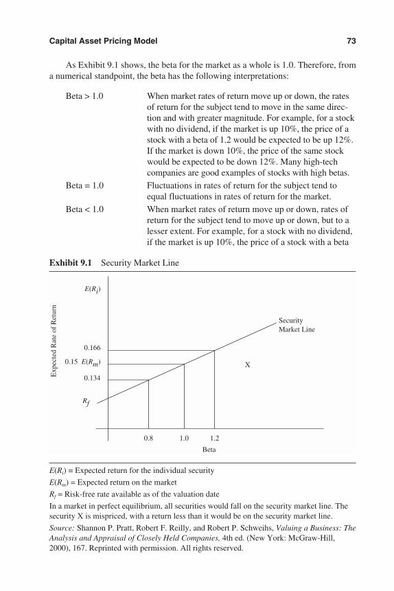
As Exhibit 9.1 shows, the beta for the market as a whole is 1.0. Therefore, froma numerical standpoint, the beta has the following interpretations:
Beta > 1.0 When market rates of return move up or down, the ratesof return for the subject tend to move in the same direc-tion and with greater magnitude. For example, for a stockwith no dividend, if the market is up 10%, the price of astock with a beta of 1.2 would be expected to be up 12%.If the market is down 10%, the price of the same stockwould be expected to be down 12%. Many high-techcompanies are good examples of stocks with high betas.
Beta = 1.0 Fluctuations in rates of return for the subject tend toequal fluctuations in rates of return for the market.
Beta < 1.0 When market rates of return move up or down, rates ofreturn for the subject tend to move up or down, but to alesser extent. For example, for a stock with no dividend,if the market is up 10%, the price of a stock with a beta
Capital Asset Pricing Model 73
Exhibit 9.1 Security Market Line
E(Ri) = Expected return for the individual security
E(Rm) = Expected return on the market
Rf = Risk-free rate available as of the valuation date
In a market in perfect equilibrium, all securities would fall on the security market line. Thesecurity X is mispriced, with a return less than it would be on the security market line.
Source: Shannon P. Pratt, Robert F. Reilly, and Robert P. Schweihs, Valuing a Business: TheAnalysis and Appraisal of Closely Held Companies, 4th ed. (New York: McGraw-Hill,2000), 167. Reprinted with permission. All rights reserved.
SecurityMarket Line
X
1.0
Beta
E(Ri)
Rf
0.166
Exp
ecte
d R
ate
of R
etur
n
0.15 E(Rm)
0.134
0.8 1.2
3953 P-09 8/29/02 2:22 PM Page 73
of .8 would be expected to be up 8%. The classic exam-ple of a low-beta stock would be a utility that has notdiversified into riskier activities.
Negative beta (rare) Rates of return for the subject tend to move in the oppo-site direction from changes in rates of return for themarket. Stocks with negative betas are rare. A few gold-mining companies have had negative betas in the past.
To illustrate, using the preceding formula as part of the process of estimating acompany’s cost of equity capital, consider stocks of average size, publicly traded com-panies i, j, and k, with betas of 0.8, 1.0, and 1.2, respectively; a risk-free rate in themarket of 7% (0.07) at the valuation date; and a market equity risk premium of 8%(0.08).
For company i, which is less sensitive to market movements than the averagecompany, we can substitute in Formula 9.1 as follows:
Formula 9.2
E(Ri) = 0.07 + 0.8(0.08)= 0.07 + 0.064= 0.134
Thus, the cost of equity capital for company i is estimated to be 13.4% becauseit is less risky, in terms of systematic risk, than the average stock on the market.
For company j, which has average sensitivity to market movements, we can sub-stitute in Formula 9.1 as follows:
Formula 9.3
E(Rj) = 0.07 + 1.0(0.08)= 0.07 + 0.08= 0.15
So the cost of equity capital for company j is estimated to be 15%, the estimated costof capital for the average stock, because its systematic risk is equal to the average ofthe market as a whole.
For company k, which has greater-than-average sensitivity to market movements,we can substitute in Formula 9.1 as follows:
Formula 9.4
E(Rk) = 0.07 + 1.2(0.08)= 0.07 + 0.096= 0.166
Thus, the cost of equity capital for company k is estimated to be 16.6% because it isriskier, in terms of systematic risk, than the average stock on the market.
74 Estimating the Cost of Equity Capital
3953 P-09 8/29/02 2:22 PM Page 74
Note that in the preceding pure formulation of the CAPM, the required rate of re-turn is composed of only two factors:
1. The risk-free rate
2. The market’s general equity risk premium, as modified by the beta for the sub-ject security
EXPANDING CAPM TO INCORPORATE SIZE PREMIUM ANDSPECIFIC RISK
Firm Size Phenomenon
Many empirical studies performed since CAPM was originally developed haveindicated that the realized total returns on smaller companies have been substantiallygreater over a long period of time than the original formulation of the CAPM (asgiven in Formula 9.1) would have predicted. Ibbotson Associates comments on thisphenomenon:
One of the most remarkable discoveries of modern finance is that of a relationship be-tween firm size and return. The relationship cuts across the entire size spectrum but ismost evident among smaller companies, which have higher returns on average than largerones.3
The firm size phenomenon is remarkable in several ways. First, the greater risk ofsmall stocks does not, in the context of the capital asset pricing model (CAPM), fully ac-count for their higher returns over the long term. In the CAPM, only systematic or betarisk is rewarded; small company stocks have had returns in excess of those implied bytheir betas. Second, the calendar annual return differences between small and large com-panies are serially correlated. This suggests that past annual returns may be of some valuein predicting future annual returns. Such serial correlation, or autocorrelation, is practi-cally unknown in the market for large stocks and in most other equity markets but isevident in the size premia.4
The size effect is the subject of Chapter 11.
Company-specific Risk Factor
The notion that the only component of risk that investors care about is system-atic risk is based on the assumption that all unsystematic risk can be eliminated byholding a perfectly diversified portfolio of risky assets that will, by definition, havea beta of 1.0.
Without addressing the validity of that assumption for the public markets (forthe purpose of this book), it is obviously not feasible for investors in privately heldcompanies to hold such a perfectly diversified portfolio that would eliminate all
Capital Asset Pricing Model 75
3953 P-09 8/29/02 2:22 PM Page 75
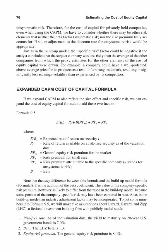
unsystematic risk. Therefore, for the cost of capital for privately held companies,even when using the CAPM, we have to consider whether there may be other riskelements that neither the beta factor (systematic risk) nor the size premium fully ac-counts for. If so, an adjustment to the discount rate for unsystematic risk would beappropriate.
Just as in the build-up model, the “specific risk” factor could be negative if theanalyst concluded that the subject company was less risky than the average of the othercompanies from which the proxy estimates for the other elements of the cost ofequity capital were drawn. For example, a company could have a well-protected,above-average price for its products as a result of a strong trademark, resulting in sig-nificantly less earnings volatility than experienced by its competitors.
EXPANDED CAPM COST OF CAPITAL FORMULA
If we expand CAPM to also reflect the size effect and specific risk, we can ex-pand the cost of equity capital formula to add these two factors:
Formula 9.5
E(Ri) = Rf + B(RPm) + RPs + RPu
where:
E(Ri) = Expected rate of return on security iRf = Rate of return available on a risk-free security as of the valuation
dateRPm = General equity risk premium for the marketRPs = Risk premium for small sizeRPu = Risk premium attributable to the specific company (u stands for
unsystematic risk)B = Beta
Note that the only difference between this formula and the build-up model formula(Formula 8.1) is the addition of the beta coefficient. The value of the company-specificrisk premium, however, is likely to differ from that used in the build-up model, becausesome portion of the company-specific risk may have been captured in beta. Also, in thebuild-up model, an industry adjustment factor may be incorporated. To put some num-bers into Formula 9.5, we will make five assumptions about Lazard, Hazard, and Zipp(LHZ), a fictional investment banking firm with publicly traded stock:
1. Risk-free rate. As of the valuation date, the yield to maturity on 20-year U.S.government bonds is 7.0%.
2. Beta. The LHZ beta is 1.3.
3. Equity risk premium. The general equity risk premium is 8.0%.
76 Estimating the Cost of Equity Capital
3953 P-09 8/29/02 2:22 PM Page 76
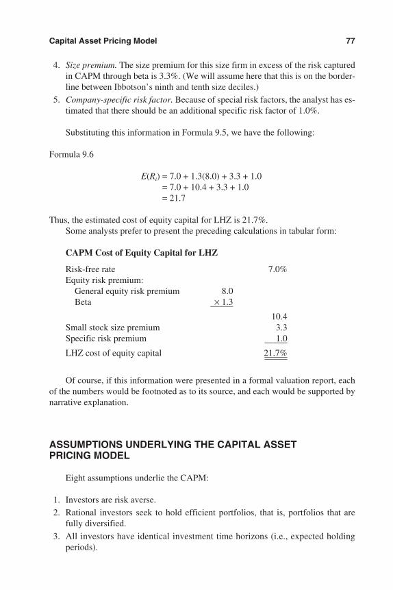
4. Size premium. The size premium for this size firm in excess of the risk capturedin CAPM through beta is 3.3%. (We will assume here that this is on the border-line between Ibbotson’s ninth and tenth size deciles.)
5. Company-specific risk factor. Because of special risk factors, the analyst has es-timated that there should be an additional specific risk factor of 1.0%.
Substituting this information in Formula 9.5, we have the following:
Formula 9.6
E(Ri) = 7.0 + 1.3(8.0) + 3.3 + 1.0= 7.0 + 10.4 + 3.3 + 1.0= 21.7
Thus, the estimated cost of equity capital for LHZ is 21.7%.Some analysts prefer to present the preceding calculations in tabular form:
CAPM Cost of Equity Capital for LHZ
Risk-free rate 7.0%Equity risk premium:
General equity risk premium 8.0Beta × 1.3——–
10.4Small stock size premium 3.3Specific risk premium 1.0—–—LHZ cost of equity capital 21.7%—–——–—
Of course, if this information were presented in a formal valuation report, eachof the numbers would be footnoted as to its source, and each would be supported bynarrative explanation.
ASSUMPTIONS UNDERLYING THE CAPITAL ASSET PRICING MODEL
Eight assumptions underlie the CAPM:
1. Investors are risk averse.
2. Rational investors seek to hold efficient portfolios, that is, portfolios that arefully diversified.
3. All investors have identical investment time horizons (i.e., expected holdingperiods).
Capital Asset Pricing Model 77
3953 P-09 8/29/02 2:22 PM Page 77
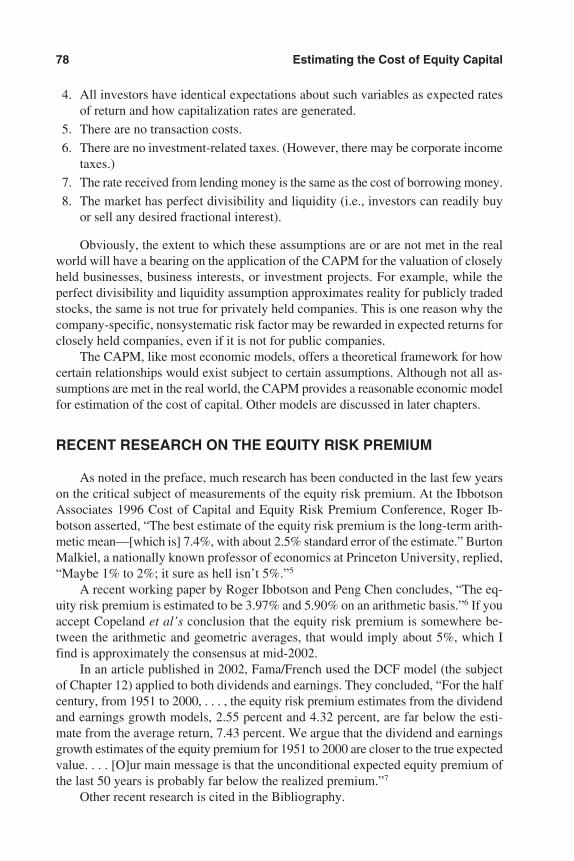
4. All investors have identical expectations about such variables as expected ratesof return and how capitalization rates are generated.
5. There are no transaction costs.
6. There are no investment-related taxes. (However, there may be corporate incometaxes.)
7. The rate received from lending money is the same as the cost of borrowing money.
8. The market has perfect divisibility and liquidity (i.e., investors can readily buyor sell any desired fractional interest).
Obviously, the extent to which these assumptions are or are not met in the realworld will have a bearing on the application of the CAPM for the valuation of closelyheld businesses, business interests, or investment projects. For example, while theperfect divisibility and liquidity assumption approximates reality for publicly tradedstocks, the same is not true for privately held companies. This is one reason why thecompany-specific, nonsystematic risk factor may be rewarded in expected returns forclosely held companies, even if it is not for public companies.
The CAPM, like most economic models, offers a theoretical framework for howcertain relationships would exist subject to certain assumptions. Although not all as-sumptions are met in the real world, the CAPM provides a reasonable economic modelfor estimation of the cost of capital. Other models are discussed in later chapters.
RECENT RESEARCH ON THE EQUITY RISK PREMIUM
As noted in the preface, much research has been conducted in the last few yearson the critical subject of measurements of the equity risk premium. At the IbbotsonAssociates 1996 Cost of Capital and Equity Risk Premium Conference, Roger Ib-botson asserted, “The best estimate of the equity risk premium is the long-term arith-metic mean—[which is] 7.4%, with about 2.5% standard error of the estimate.” BurtonMalkiel, a nationally known professor of economics at Princeton University, replied,“Maybe 1% to 2%; it sure as hell isn’t 5%.”5
A recent working paper by Roger Ibbotson and Peng Chen concludes, “The eq-uity risk premium is estimated to be 3.97% and 5.90% on an arithmetic basis.”6 If youaccept Copeland et al’s conclusion that the equity risk premium is somewhere be-tween the arithmetic and geometric averages, that would imply about 5%, which Ifind is approximately the consensus at mid-2002.
In an article published in 2002, Fama/French used the DCF model (the subjectof Chapter 12) applied to both dividends and earnings. They concluded, “For the halfcentury, from 1951 to 2000, . . . , the equity risk premium estimates from the dividendand earnings growth models, 2.55 percent and 4.32 percent, are far below the esti-mate from the average return, 7.43 percent. We argue that the dividend and earningsgrowth estimates of the equity premium for 1951 to 2000 are closer to the true expectedvalue. . . . [O]ur main message is that the unconditional expected equity premium ofthe last 50 years is probably far below the realized premium.”7
Other recent research is cited in the Bibliography.
78 Estimating the Cost of Equity Capital
3953 P-09 8/29/02 2:22 PM Page 78
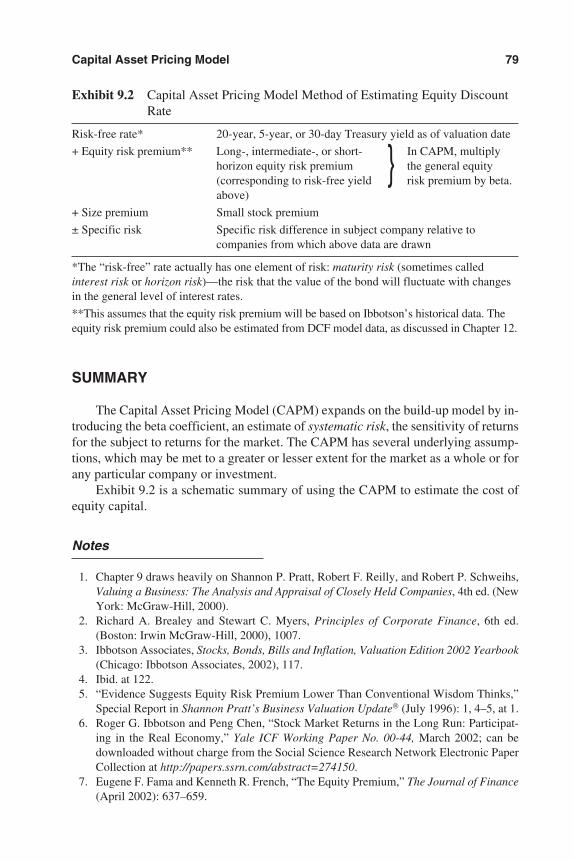
Exhibit 9.2 Capital Asset Pricing Model Method of Estimating Equity DiscountRate
Risk-free rate* 20-year, 5-year, or 30-day Treasury yield as of valuation date
+ Equity risk premium** Long-, intermediate-, or short- In CAPM, multiply horizon equity risk premium the general equity (corresponding to risk-free yield risk premium by beta.above)
+ Size premium Small stock premium
± Specific risk Specific risk difference in subject company relative tocompanies from which above data are drawn
*The “risk-free” rate actually has one element of risk: maturity risk (sometimes calledinterest risk or horizon risk)—the risk that the value of the bond will fluctuate with changesin the general level of interest rates.
**This assumes that the equity risk premium will be based on Ibbotson’s historical data. Theequity risk premium could also be estimated from DCF model data, as discussed in Chapter 12.
SUMMARY
The Capital Asset Pricing Model (CAPM) expands on the build-up model by in-troducing the beta coefficient, an estimate of systematic risk, the sensitivity of returnsfor the subject to returns for the market. The CAPM has several underlying assump-tions, which may be met to a greater or lesser extent for the market as a whole or forany particular company or investment.
Exhibit 9.2 is a schematic summary of using the CAPM to estimate the cost ofequity capital.
Notes
1. Chapter 9 draws heavily on Shannon P. Pratt, Robert F. Reilly, and Robert P. Schweihs,Valuing a Business: The Analysis and Appraisal of Closely Held Companies, 4th ed. (NewYork: McGraw-Hill, 2000).
2. Richard A. Brealey and Stewart C. Myers, Principles of Corporate Finance, 6th ed.(Boston: Irwin McGraw-Hill, 2000), 1007.
3. Ibbotson Associates, Stocks, Bonds, Bills and Inflation, Valuation Edition 2002 Yearbook(Chicago: Ibbotson Associates, 2002), 117.
4. Ibid. at 122.5. “Evidence Suggests Equity Risk Premium Lower Than Conventional Wisdom Thinks,”
Special Report in Shannon Pratt’s Business Valuation Update (July 1996): 1, 4–5, at 1.6. Roger G. Ibbotson and Peng Chen, “Stock Market Returns in the Long Run: Participat-
ing in the Real Economy,” Yale ICF Working Paper No. 00-44, March 2002; can bedownloaded without charge from the Social Science Research Network Electronic PaperCollection at http://papers.ssrn.com/abstract=274150.
7. Eugene F. Fama and Kenneth R. French, “The Equity Premium,” The Journal of Finance(April 2002): 637–659.
Capital Asset Pricing Model 79
}
3953 P-09 8/29/02 2:22 PM Page 79
80
Chapter 10
Proper Use of BetasEstimation of BetaDifferences in Estimation of Beta
Length of the Measurement PeriodFrequency of Data MeasurementChoice of Market IndexChoice of Risk-free Rate
Levered and Unlevered BetasModified Betas: Shrunk and Lagged
Adjusted Beta Incorporates Industry Norm (Shrunk Beta)“Sum Beta” Incorporates Lag Effect
Summary
As discussed in the previous chapter, the beta is used as a modifier to the equityrisk premium in the context of the Capital Asset Pricing Model (CAPM). The purposeof this chapter is to explore some widely used variations in the construction and ap-plication of betas.
ESTIMATION OF BETA
Systematic risk is measured in CAPM by a factor called beta. Beta is a functionof the relationship between the return on an individual security and the return on themarket as measured by a broad market index such as the Standard & Poor’s (S&P)500 Index.
Beta often is measured by comparing the excess return on an individual securityrelative to the excess return on the market index. By excess return, we mean the totalreturn (which includes both dividends and capital gains and losses) over and abovethe return available on a risk-free investment (e.g., U.S. Treasuries).
Theorists prefer to measure beta on the basis of excess returns rather than totalreturns. However, a comparison of measurements by the two choices show that, as apractical matter, it makes little difference. Ibbotson Associates uses excess returns inall its computations.
A common method of calculating beta is to compute the slope of the best-fit linebetween the (excess) return on the individual security and the (excess) return on themarket. An example of this is shown in Exhibit 10.1.
3953 P-10 8/29/02 2:23 PM Page 80
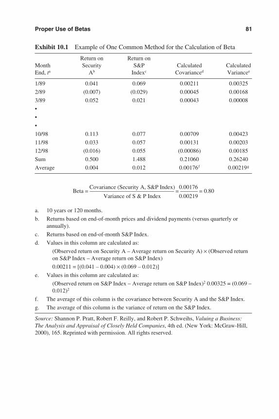
Proper Use of Betas 81
Exhibit 10.1 Example of One Common Method for the Calculation of Beta
Return on Return onMonth Security S&P Calculated CalculatedEnd, ta Ab Indexc Covarianced Variancee
1/89 0.041 0.069 0.00211 0.00325
2/89 (0.007) (0.029) 0.00045 0.00168
3/89 0.052 0.021 0.00043 0.00008
•
•
•
10/98 0.113 0.077 0.00709 0.00423
11/98 0.033 0.057 0.00131 0.00203
12/98 (0.016) 0.055 (0.00086) 0.00185
Sum 0.500 1.488 0.21060 0.26240
Average 0.004 0.012 0.00176f 0.00219g
Covariance (Security A, S&P Index) 0.00176Beta = —————————————––– = ——— = 0.80
Variance of S & P Index 0.00219
a. 10 years or 120 months.
b. Returns based on end-of-month prices and dividend payments (versus quarterly orannually).
c. Returns based on end-of-month S&P Index.
d. Values in this column are calculated as:
(Observed return on Security A – Average return on Security A) × (Observed returnon S&P Index – Average return on S&P Index)
0.00211 = [(0.041 – 0.004) × (0.069 – 0.012)]
e. Values in this column are calculated as:
(Observed return on S&P Index – Average return on S&P Index)2 0.00325 = (0.069 –0.012)2
f. The average of this column is the covariance between Security A and the S&P Index.
g. The average of this column is the variance of return on the S&P Index.
Source: Shannon P. Pratt, Robert F. Reilly, and Robert P. Schweihs, Valuing a Business:The Analysis and Appraisal of Closely Held Companies, 4th ed. (New York: McGraw-Hill,2000), 165. Reprinted with permission. All rights reserved.
3953 P-10 8/29/02 2:23 PM Page 81
Because we cannot compute a beta directly for a privately held company, as notedin Chapter 9, we go to reference sources to obtain betas for guideline public compa-nies or industries to determine a proxy beta for our private company. Details on thesesources can be found in Appendix C.
DIFFERENCES IN ESTIMATION OF BETA
Be aware that significant differences exist between betas for the same stock pub-lished by different financial reporting services. One of the implications of this fact isthat betas for guideline companies used in a valuation should all come from the samesource. If all betas for guideline companies are not available from a single source, thebest solution is probably to use the source providing betas for the greatest number ofguideline companies and not use betas given for the others. Otherwise an “apples andoranges” mixture will result.
Differences in the beta measurement derive from choices within four variables:
1. The length of the total time period over which the returns are measured
2. The periodicity (frequency) of measurement within that time period
3. The choice of an index to use as a market proxy
4. The risk-free rate above which the excess returns should be measured
In addition to how these four variables are treated, adjustments can be made torecognize the beta’s tendency to adjust toward 1.0. These adjustments are discussedlater in the chapter.
Length of the Measurement Period
Most services that calculate beta use a two- to five-year measurement period, withfive years being the most common. The Ibbotson Associates Beta Book uses 60 monthsfor most stocks but includes a beta based on as few as 36 months if data are avail-able for only this length of time.
Frequency of Data Measurement
Data may be measured daily, weekly, monthly, quarterly, or annually. Monthly isthe most common frequency, although Value Line uses five years of weekly data.
Choice of Market Index
The market index used in calculating beta could be any of the following or, insome cases, another index:
82 Estimating the Cost of Equity Capital
3953 P-10 8/29/02 2:23 PM Page 82
• Standard & Poor’s (S&P) 500 Index
• New York Stock Exchange (NYSE) Composite Index
• NYSE and American Stock Exchange (AMEX)
• NYSE, AMEX, and over-the-counter (OTC)
• Value Line Index
For an index to be representative of the market, it must be market-capitalizationweighted. That is, the weight for each company in the index is determined by the mar-ket value of its equity. The sizes of the companies in the S&P 500 Index are so greatthat the index comprises about 70% of the total capitalization of all of the stock con-stituting the combined indexes listed here. Furthermore, the broader market indexesshown above correlate almost perfectly with the S&P 500 Index.
As a result, it does not make a great deal of difference which index is used. Ibbot-son uses the NYSE in its calculations for the Cost of Capital Yearbook and the BetaBook.
Choice of Risk-free Rate
To avoid the maturity risk (interest rate risk) inherent in long-term bonds, the risk-free rate used to compute excess returns generally is either the Treasury-bill rate or theincome return only from Treasury bonds. Ibbotson uses the 30-day Treasury bill in itscalculations for the Cost of Capital Yearbook and the Beta Book.
A list of sources for betas is included in Appendix C.
LEVERED AND UNLEVERED BETAS
Published betas for publicly traded stocks typically reflect the capital structure ofeach respective company. These betas are sometimes referred to as levered betas, betasreflecting the leverage in the company’s capital structure. If the leverage of the com-pany subject to appraisal differs significantly from the leverage of the guideline com-panies selected for analysis, or if the debt levels of the guideline companies differsignificantly from one another, it may be desirable to remove the effect that leveragehas on the betas before using them as a proxy to estimate the beta of the subject.
When the firm’s beta is measured based on observed historical total returns (asmost betas are), its measurement necessarily includes volatility related to the com-pany’s financial risk. In particular, the equity of companies with higher levels of debtis riskier than the equity of companies with less leverage (all else being equal). In otherwords, levered betas incorporate two risk factors that bear on systematic risk: businessrisk and financial (or capital structure) risk.
This adjustment for leverage differences is performed by first computing unlev-ered betas for the guideline companies. An unlevered beta is the beta a company would
Proper Use of Betas 83
3953 P-10 8/29/02 2:23 PM Page 83
have if it had no debt. The second step is to decide where the subject company’s riskwould fall on an unlevered basis relative to the guideline companies. The third andfinal step is to relever the beta for the subject company on the basis of one or more as-sumed capital structures. The result will be a market-derived beta specifically adjustedfor the degree of financial leverage of the subject company.
To summarize, the three steps are:
1. Compute an unlevered beta for each of the guideline companies.
2. Decide where the risk would fall for the subject company relative to the guidelinecompanies, assuming all had 100% equity capital structures.
3. Relever the beta for the subject company based on one or more assumed capitalstructures.
The formulas and an example of this process are shown in Exhibit 10.2. Of course,this leverage adjustment procedure takes as given all the assumptions of the CapitalAsset Pricing Model.
With respect to levered versus unlevered betas, the capital structure of compa-nies often can change significantly over the measurement period of the beta. For ex-ample, a beta could be measured during a five-year period in which, for the majorityof time, a company was unleveraged. If at the end of the five-year measurement pe-riod the company has become highly leveraged, the levered betas computed wouldincorporate very little leverage. Yet in unlevering the beta, the analyst would incor-porate the current level of high leverage. Thus the unlevered beta could be highly un-derestimated. The reverse effect applies for a company that deleverages during thebeta measurement period. There is no specific method of correcting for this other thanaccounting for capital structure changes when unlevering the beta. A reasonable ap-proach might be to determine the average leverage for the company during the betameasurement period rather than the leverage at the end of the measurement period.
Capital structures for both the guideline companies and the subject companiesare assumed to be based on market values in this process. If the relevered beta is usedto estimate the market value of a company on a controlling basis, and if it is antici-pated that the actual capital structure will be adjusted to the proportions of debt andequity in the assumed capital structure, then only one assumed capital structure isnecessary. However, if the amount of debt in the subject capital structure will not beadjusted, an iterative process may be required. The initial assumed capital structurefor the subject will influence the cost of equity, which will, in turn, influence the rel-ative proportions of debt and equity at market value. It may be necessary to try sev-eral assumed capital structures until one of them produces an estimate of equity valuethat actually results in the assumed capital structure.
This process of unlevering and relevering betas to an assumed capital structureis based on the assumption that the subject business interest has the ability to changethe capital structure of the subject company. In the case of the valuation of a minor-ity ownership interest, for example, the subject business interest may not have thatability.1
84 Estimating the Cost of Equity Capital
3953 P-10 8/29/02 2:23 PM Page 84
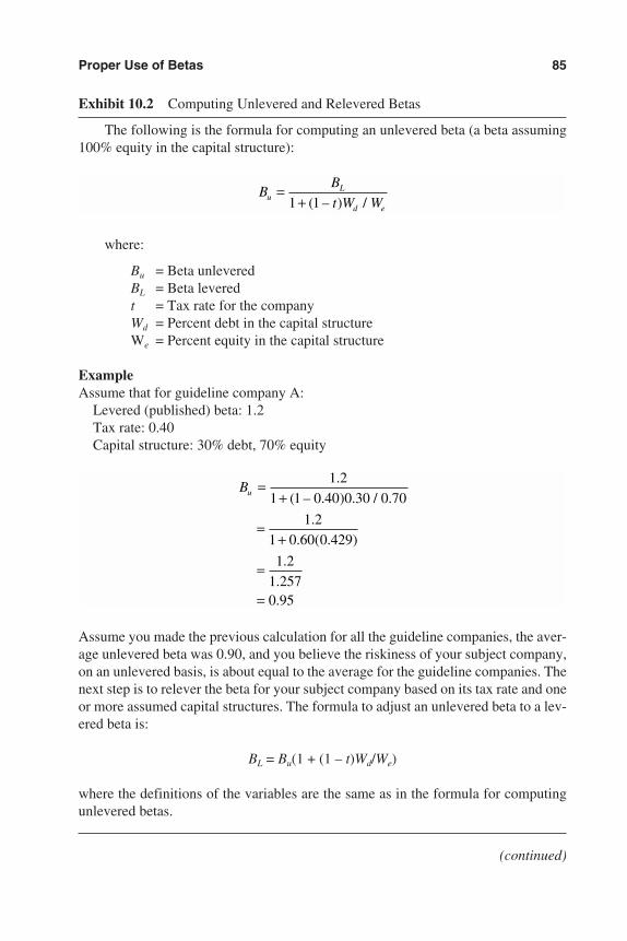
Proper Use of Betas 85
Exhibit 10.2 Computing Unlevered and Relevered Betas
The following is the formula for computing an unlevered beta (a beta assuming100% equity in the capital structure):
where:
Bu = Beta unleveredBL = Beta leveredt = Tax rate for the companyWd = Percent debt in the capital structureWe = Percent equity in the capital structure
ExampleAssume that for guideline company A:
Levered (published) beta: 1.2Tax rate: 0.40Capital structure: 30% debt, 70% equity
Assume you made the previous calculation for all the guideline companies, the aver-age unlevered beta was 0.90, and you believe the riskiness of your subject company,on an unlevered basis, is about equal to the average for the guideline companies. Thenext step is to relever the beta for your subject company based on its tax rate and oneor more assumed capital structures. The formula to adjust an unlevered beta to a lev-ered beta is:
BL = Bu(1 + (1 – t)Wd/We)
where the definitions of the variables are the same as in the formula for computingunlevered betas.
Bu =+
=+
=
=
1 2
1 1 0 40 0 30 0 70
1 2
1 0 60 0 429
1 2
1 2570 95
.
( – . ) . / .
.
. ( . )
.
.
.
BB
t W WuL
d e
=+1 1( – ) /
(continued)
3953 P-10 8/29/02 2:23 PM Page 85
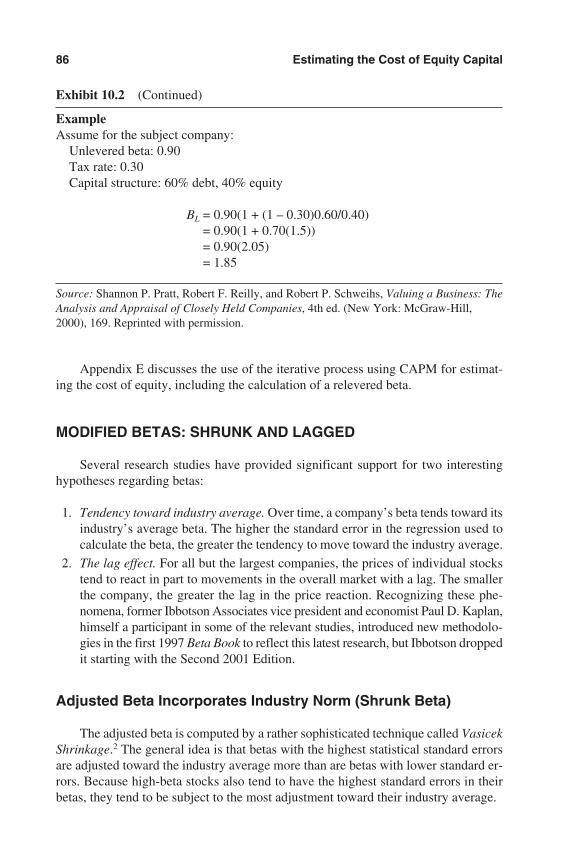
Appendix E discusses the use of the iterative process using CAPM for estimat-ing the cost of equity, including the calculation of a relevered beta.
MODIFIED BETAS: SHRUNK AND LAGGED
Several research studies have provided significant support for two interestinghypotheses regarding betas:
1. Tendency toward industry average. Over time, a company’s beta tends toward itsindustry’s average beta. The higher the standard error in the regression used tocalculate the beta, the greater the tendency to move toward the industry average.
2. The lag effect. For all but the largest companies, the prices of individual stockstend to react in part to movements in the overall market with a lag. The smallerthe company, the greater the lag in the price reaction. Recognizing these phe-nomena, former Ibbotson Associates vice president and economist Paul D. Kaplan,himself a participant in some of the relevant studies, introduced new methodolo-gies in the first 1997 Beta Book to reflect this latest research, but Ibbotson droppedit starting with the Second 2001 Edition.
Adjusted Beta Incorporates Industry Norm (Shrunk Beta)
The adjusted beta is computed by a rather sophisticated technique called VasicekShrinkage.2 The general idea is that betas with the highest statistical standard errorsare adjusted toward the industry average more than are betas with lower standard er-rors. Because high-beta stocks also tend to have the highest standard errors in theirbetas, they tend to be subject to the most adjustment toward their industry average.
86 Estimating the Cost of Equity Capital
Exhibit 10.2 (Continued)
ExampleAssume for the subject company:
Unlevered beta: 0.90Tax rate: 0.30Capital structure: 60% debt, 40% equity
BL = 0.90(1 + (1 – 0.30)0.60/0.40)= 0.90(1 + 0.70(1.5))= 0.90(2.05)= 1.85
Source: Shannon P. Pratt, Robert F. Reilly, and Robert P. Schweihs, Valuing a Business: TheAnalysis and Appraisal of Closely Held Companies, 4th ed. (New York: McGraw-Hill,2000), 169. Reprinted with permission.
3953 P-10 8/29/02 2:23 PM Page 86
“Sum Beta” Incorporates Lag Effect
Because of the lag in all but the largest companies’ sensitivity to movements inthe overall market, traditional betas tend to understate systematic risk. As the First2001 Edition of the Beta Book explains it, “Because of nonsynchronous price reac-tions, the traditional betas estimated by ordinary least squares are biased down for allbut the largest companies.”3 As noted above, however, the Second 2001 Edition dis-continued presentation of sum betas.
The research suggests that this understatement of systematic risk by the tradi-tional beta measurements accounts in part, but certainly not wholly, for the fact thatsmall stocks achieve excess returns over their apparent Capital Asset Pricing Model-required returns (where the market equity risk premium is adjusted for beta).
A sum beta consists of a multiple regression of a stock’s current month’s excessreturns over the 30-day Treasury-bill rate on the market’s current month’s excess re-turns and on the market’s previous month’s excess returns, and then a summing of thecoefficients. This helps to capture more fully the lagged effect of comovement in acompany’s returns with returns on the market (systematic risk).4
Exhibit 10.3 is an excerpt from Ibbotson’s Second 2001 Edition Beta Book(which is published twice annually). Note that it includes a traditional least squaresregression beta and the Fama-French three-factor models.
Chapter 13 on using Ibbotson data shows an entire sample page from the Second2001 Edition Beta Book.
The 2002 SBBI Valuation Edition has a table (Table 7-7) titled “Long-term Returnin Excess of CAPM for Decile Portfolios of the NYSE/AMEX/NASDAQ, with SumBeta.”5 The returns in excess of CAPM are much lower than for the ordinary leastsquares (OLS) betas, reflecting the superiority of sum betas over OLS betas. Graph7-4 on the same page shows how much closer the portfolios track the Security MarketLine, except for the tenth decile.6 If sum betas are used, the size premium in excessof CAPM is greatly reduced.
Sum betas for individual stocks can be calculated using an Excel spreadsheet and61 months of performance data, which is available from several sources, such asCOMPUSTAT. Thus, even though the sum betas have been removed from the BetaBook, some analysts prefer to calculate their own sum betas for a peer group of pub-lic companies (which they use as a proxy for the beta of their subject private companyin the context of CAPM), and thus make a smaller adjustment for the size effect. Thetheory is that this corrects for the larger size effect that is principally due to a misspec-ification of beta when using traditional OLS betas for the smaller companies.
SUMMARY
A beta is a measure of the sensitivity of the movement in returns on a particularstock to movements in returns on some measure of the market. As such, beta measuressystematic risk. In cost of capital estimation, beta is used as a modifier to the generalequity risk premium in using the Capital Asset Pricing Model.
Proper Use of Betas 87
3953 P-10 8/29/02 2:23 PM Page 87
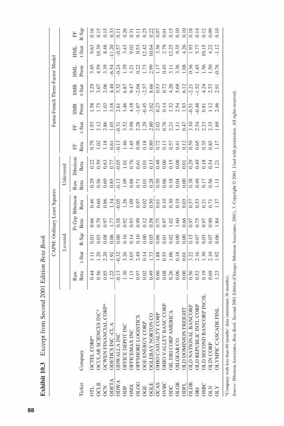
88
Exh
ibit
10.
3E
xcer
pt f
rom
Sec
ond
2001
Edi
tion
Bet
a B
ook
CA
PM: O
rdin
ary
Lea
st S
quar
esFa
ma-
Fren
ch T
hree
-Fac
tor
Mod
el
Lev
ered
Unl
ever
ed
Raw
Pr G
rpIb
bots
onR
awIb
bots
onFF
FFSM
BSM
BH
ML
HM
LFF
Tic
ker
Com
pany
Bet
at-
Stat
R-S
qrB
eta
Bet
aB
eta
Bet
aB
eta
t-St
atPr
emt-
Stat
Prem
t-St
atR
-Sqr
OT
LO
CT
EL
CO
RP*
0.44
1.11
0.03
0.66
0.46
0.29
0.22
0.79
1.93
1.58
3.29
3.45
9.63
0.16
OC
LR
OC
UL
AR
SC
IEN
CE
S IN
C*
0.56
1.20
0.03
0.79
0.60
0.56
0.59
1.02
2.12
1.75
3.07
4.59
10.3
90.
15O
CN
OC
WE
N F
INA
NC
IAL
CO
RP*
0.85
2.20
0.08
0.97
0.86
0.69
0.63
1.18
2.86
1.03
2.06
3.39
8.48
0.15
OD
ET
AO
DE
TIC
S IN
C -
CL
A1.
221.
920.
061.
771.
340.
850.
770.
611.
033.
184.
40–6
.54
–11.
200.
33—
——
——
——
——
——
——
——
——
——
–——
——
——
——
——
——
——
——
——
——
——
——
——
——
——
——
——
——
——
——
——
——
——
——
——
–O
DW
AO
DW
AL
LA
IN
C–0
.13
–0.3
20.
000.
58–0
.05
–0.1
3–0
.05
–0.1
3–0
.31
2.81
5.32
–0.2
4–0
.57
0.11
OD
PO
FFIC
E D
EPO
T I
NC
1.30
3.26
0.16
0.92
1.26
1.09
1.01
1.46
3.52
3.46
6.87
1.39
3.43
0.26
OM
XO
FFIC
EM
AX
IN
C1.
113.
030.
140.
931.
090.
880.
761.
453.
984.
189.
473.
219.
020.
31O
LO
GO
FFSH
OR
E L
OG
IST
ICS
0.97
2.49
0.10
0.99
0.97
0.71
0.61
0.98
2.28
–1.0
7–2
.04
0.22
0.53
0.11
OG
EO
GE
EN
ER
GY
CO
RP
0.02
0.14
0.00
0.12
0.02
0.01
0.01
0.18
1.29
–0.4
5–2
.57
1.73
12.4
20.
25O
GL
EO
GL
EB
AY
NO
RT
ON
CO
0.49
1.73
0.05
0.58
0.50
0.28
0.13
0.80
2.80
3.02
8.66
2.99
10.6
40.
22—
——
——
——
——
——
——
——
——
——
–——
——
——
——
——
——
——
——
——
——
——
——
——
——
——
——
——
——
——
——
——
——
——
——
——
–O
CA
SO
HIO
CA
SUA
LT
Y C
OR
P0.
601.
880.
060.
750.
610.
500.
480.
722.
020.
230.
531.
173.
360.
07O
VB
CO
HIO
VA
LL
EY
BA
NC
CO
RP
0.08
0.55
0.01
0.97
0.10
0.06
0.06
0.13
0.76
0.14
0.72
0.45
2.79
0.01
OD
CO
IL D
RI
CO
RP
AM
ER
ICA
0.26
1.06
0.02
1.02
0.30
0.18
0.15
0.57
2.21
1.32
4.20
3.11
12.2
50.
15O
LG
RO
ILG
EA
R C
O0.
060.
180.
001.
600.
190.
040.
080.
411.
112.
545.
693.
369.
350.
10O
DFL
OL
D D
OM
INIO
N F
RE
IGH
T0.
000.
010.
000.
660.
030.
000.
010.
120.
471.
936.
121.
084.
260.
10—
——
——
——
——
——
——
——
——
——
–——
——
——
——
——
——
——
——
——
——
——
——
——
——
——
——
——
——
——
——
——
——
——
——
——
–O
LD
BO
LD
NA
TIO
NA
L B
AN
CO
RP
0.56
3.22
0.15
0.97
0.57
0.38
0.29
0.59
3.10
–0.5
1–2
.21
0.36
1.93
0.18
OR
IO
LD
RE
PUB
LIC
IN
TL
CO
RP
0.52
2.16
0.07
0.75
0.53
0.49
0.49
0.65
2.54
–0.4
8–1
.52
1.45
5.77
0.14
OSB
CO
LD
SE
CO
ND
BA
NC
OR
P IN
C/I
L0.
191.
300.
030.
970.
210.
170.
180.
352.
230.
814.
241.
5610
.15
0.12
OL
NO
LIN
CO
RP
0.69
2.10
0.07
0.90
0.71
0.56
0.54
0.85
2.33
1.12
2.53
1.50
4.22
0.09
OL
YO
LY
MPI
C C
ASC
AD
E F
INL
1.23
1.92
0.06
1.84
1.37
1.11
1.21
1.17
1.69
2.46
2.91
–0.7
6–1
.12
0.10
*Com
pany
with
less
than
60
mon
ths’
dat
a (m
inim
um 3
6 m
onth
s).
Sour
ce:
Ibbo
tson
Ass
ocia
tes,
Bet
a B
ook,
Sec
ond
2001
Edi
tion
(Chi
cago
: Ibb
otso
n A
ssoc
iate
s, 2
001)
, 3. C
opyr
ight
©20
01. U
sed
with
per
mis
sion
. All
righ
ts r
eser
ved.
3953 P-10 8/29/02 2:23 PM Page 88
There are many variations on the way betas are measured by different sources ofpublished betas. Thus, a beta for a stock computed by one source may be very differ-ent from a beta computed for the same stock by another source.
Modern research is attempting to improve betas. Two such improvements im-plemented are the “shrunk beta,” which blends the individual stock beta with the in-dustry beta, and the “lagged beta,” also called the “sum beta,” which blends the betafor the stock and the market during a concurrent time period with a beta regressedon the market’s previous period returns. These two adjustments both help to reduce“outliers,” thus perhaps making the betas based on observed historical data a littlemore representative of future expectations. The size premium in excess of CAPM ismuch lower using sum betas.
Notes
1. This section has assumed beta of debt is zero. Actually, debt tends to have betas of about0.2 to 0.3, slightly alleviating the unlevered/levered beta differential.
2. The formula, used in the Ibbotson Beta Book, was first suggested by Oldrich A. Vasicek,“A Note on Using Cross-Sectional Information in Bayesian Estimation of Security Prices,”Journal of Finance (1973). The company beta and the peer group (industry) beta areweighted. The greater the statistical confidence in the company beta, the greater the weighton the company beta relative to the peer group beta.
3. Ibbotson Associates, Beta Book, Second 2001 Edition (Chicago: Ibbotson Associates,2001), vi.
4. The sum beta estimates conform with the expectation that betas are higher for lower cap-italization stocks. Research also shows that sum betas are positively related to subsequentrealized returns over a long period of time; see Roger G. Ibbotson, Paul D. Kaplan, andJames D. Peterson, “Estimates of Small-Stock Betas Are Much Too Low,” Journal of Port-folio Management (summer 1997).
5. Ibbotson Associates, Stocks, Bonds, Bills and Inflation, Valuation Edition 2002 Yearbook(Chicago: Ibbotson Associates, 2002), 129.
6. Ibid.
Proper Use of Betas 89
3953 P-10 8/29/02 2:23 PM Page 89
90
Chapter 11
Size EffectIbbotson Associates StudiesStandard & Poor’s Corporate Value Consulting Studies (formerly the
PricewaterhouseCoopers Studies)Twenty-five Size Categories, Eight Measures of SizeUse of Measures of Risk from Company Financial Statements
Extension of Data to Smaller Size Categories: Results from the Pratt’s Stats™Database
Summary
In the chapters on the build-up and the Capital Asset Pricing Model (CAPM) costof equity estimation models, we have made reference to the “size effect,” the generalidea that smaller size is associated with higher risk and, therefore, higher cost of cap-ital. To help quantify the size effect in terms of its impact on cost of equity capital, thischapter presents empirical data from two independent sets of studies:
1. Ibbotson Associates Studies
2. Standard & Poor’s Corporate Value Consulting Studies (formerly the Pricewater-houseCoopers studies)
Both of these sets of studies use rate of return data developed at the University ofChicago Center for Research in Security Prices (CRSP).
In addition, this chapter presents a comparative valuation multiple study of smallcompanies from data on Pratt’s Stats™, a database of private company sales.
IBBOTSON ASSOCIATES STUDIES
For many years, Ibbotson Associates has broken down New York Stock Exchange(NYSE) stock returns into quintiles by size, as measured by the aggregate market valueof the common equity. Recently Ibbotson has further refined the breakdowns intodecile groups. The excess returns over the basic general equity risk premium increasedramatically with decreasing size, as shown in Exhibit 11.1. This excess return is es-pecially noticeable for the smallest 10% of the companies. Exhibit 11.2 shows the mar-ket capitalization by value of company equity of the largest company in each of therespective decile groups as of September 30, 2000.
3953 P-11 8/29/02 2:23 PM Page 90
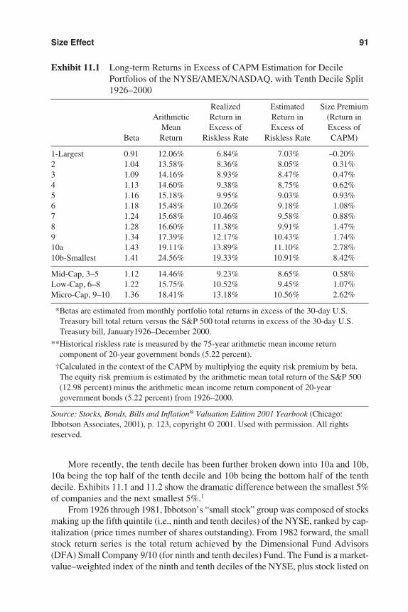
More recently, the tenth decile has been further broken down into 10a and 10b,10a being the top half of the tenth decile and 10b being the bottom half of the tenthdecile. Exhibits 11.1 and 11.2 show the dramatic difference between the smallest 5%of companies and the next smallest 5%.1
From 1926 through 1981, Ibbotson’s “small stock” group was composed of stocksmaking up the fifth quintile (i.e., ninth and tenth deciles) of the NYSE, ranked by cap-italization (price times number of shares outstanding). From 1982 forward, the smallstock return series is the total return achieved by the Dimensional Fund Advisors(DFA) Small Company 9/10 (for ninth and tenth deciles) Fund. The Fund is a market-value–weighted index of the ninth and tenth deciles of the NYSE, plus stock listed on
Size Effect 91
Exhibit 11.1 Long-term Returns in Excess of CAPM Estimation for DecilePortfolios of the NYSE/AMEX/NASDAQ, with Tenth Decile Split1926–2000
Realized Estimated Size PremiumArithmetic Return in Return in (Return in
Mean Excess of Excess of Excess ofBeta Return Riskless Rate Riskless Rate CAPM)
1-Largest 0.91 12.06% 6.84% 7.03% –0.20%2 1.04 13.58% 8.36% 8.05% 0.31%3 1.09 14.16% 8.93% 8.47% 0.47%4 1.13 14.60% 9.38% 8.75% 0.62%5 1.16 15.18% 9.95% 9.03% 0.93%6 1.18 15.48% 10.26% 9.18% 1.08%7 1.24 15.68% 10.46% 9.58% 0.88%8 1.28 16.60% 11.38% 9.91% 1.47%9 1.34 17.39% 12.17% 10.43% 1.74%10a 1.43 19.11% 13.89% 11.10% 2.78%10b-Smallest 1.41 24.56% 19.33% 10.91% 8.42%
Mid-Cap, 3–5 1.12 14.46% 9.23% 8.65% 0.58%Low-Cap, 6–8 1.22 15.75% 10.52% 9.45% 1.07%Micro-Cap, 9–10 1.36 18.41% 13.18% 10.56% 2.62%
*Betas are estimated from monthly portfolio total returns in excess of the 30-day U.S.Treasury bill total return versus the S&P 500 total returns in excess of the 30-day U.S.Treasury bill, January1926–December 2000.
**Historical riskless rate is measured by the 75-year arithmetic mean income returncomponent of 20-year government bonds (5.22 percent).
†Calculated in the context of the CAPM by multiplying the equity risk premium by beta.The equity risk premium is estimated by the arithmetic mean total return of the S&P 500(12.98 percent) minus the arithmetic mean income return component of 20-yeargovernment bonds (5.22 percent) from 1926–2000.
Source: Stocks, Bonds, Bills and Inflation® Valuation Edition 2001 Yearbook (Chicago:Ibbotson Associates, 2001), p. 123, copyright © 2001. Used with permission. All rightsreserved.
3953 P-11 8/29/02 2:23 PM Page 91
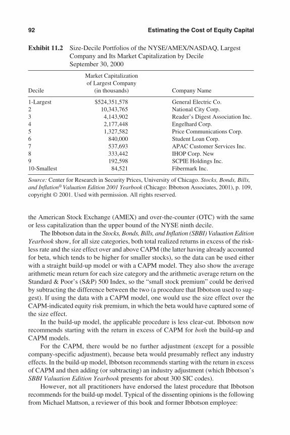
the American Stock Exchange (AMEX) and over-the-counter (OTC) with the sameor less capitalization than the upper bound of the NYSE ninth decile.
The Ibbotson data in the Stocks, Bonds, Bills, and Inflation (SBBI) Valuation EditionYearbook show, for all size categories, both total realized returns in excess of the risk-less rate and the size effect over and above CAPM (the latter having already accountedfor beta, which tends to be higher for smaller stocks), so the data can be used eitherwith a straight build-up model or with a CAPM model. They also show the averagearithmetic mean return for each size category and the arithmetic average return on theStandard & Poor’s (S&P) 500 Index, so the “small stock premium” could be derivedby subtracting the difference between the two (a procedure that Ibbotson used to sug-gest). If using the data with a CAPM model, one would use the size effect over theCAPM-indicated equity risk premium, in which the beta would have captured some ofthe size effect.
In the build-up model, the applicable procedure is less clear-cut. Ibbotson nowrecommends starting with the return in excess of CAPM for both the build-up andCAPM models.
For the CAPM, there would be no further adjustment (except for a possiblecompany-specific adjustment), because beta would presumably reflect any industryeffects. In the build-up model, Ibbotson recommends starting with the return in excessof CAPM and then adding (or subtracting) an industry adjustment (which Ibbotson’sSBBI Valuation Edition Yearbook presents for about 300 SIC codes).
However, not all practitioners have endorsed the latest procedure that Ibbotsonrecommends for the build-up model. Typical of the dissenting opinions is the followingfrom Michael Mattson, a reviewer of this book and former Ibbotson employee:
92 Estimating the Cost of Equity Capital
Exhibit 11.2 Size-Decile Portfolios of the NYSE/AMEX/NASDAQ, LargestCompany and Its Market Capitalization by DecileSeptember 30, 2000
Market Capitalizationof Largest Company
Decile (in thousands) Company Name
1-Largest $524,351,578 General Electric Co.2 10,343,765 National City Corp.3 4,143,902 Reader’s Digest Association Inc.4 2,177,448 Engelhard Corp.5 1,327,582 Price Communications Corp.6 840,000 Student Loan Corp.7 537,693 APAC Customer Services Inc.8 333,442 IHOP Corp. New9 192,598 SCPIE Holdings Inc.10-Smallest 84,521 Fibermark Inc.
Source: Center for Research in Security Prices, University of Chicago. Stocks, Bonds, Bills,and Inflation® Valuation Edition 2001 Yearbook (Chicago: Ibbotson Associates, 2001), p. 109,copyright © 2001. Used with permission. All rights reserved.
3953 P-11 8/29/02 2:23 PM Page 92
I am not in agreement with Ibbotson’s contention that the only size premium to use isthe one that is “beta adjusted.” The problem in the build-up approach is that we have noplace for a beta, so the aspect of size that is captured by a higher beta—an additional 0.4over the market beta of 1.0 for 10th decile stocks—is not captured anywhere. Using thefull size premium, as opposed to the beta-adjusted one, assumes that the small companybeing valued has similar risk characteristics to the average 10th decile company—this maynot be such a bad assumption for many of the companies we value. Assuming that 10thdecile companies are not in riskier industries than companies in the other size groupings,then their higher beta is due primarily to their size and the size effect is in both the betaand the premium over the CAPM line.
I’m not persuaded that the industry premium would be anything other than anotherfactor in the buildup model. The final problem with using just beta-adjusted size premiumin the build-up model is that, absent an alpha, you would never come up with a discountrate as high as the historical average rate of return on small stocks. Is there any reason tobelieve that the differential between small and large stocks has actually shrunken overthe last 75 years? Historically the difference between companies in the decile 1 and thosein 10b have been 13.1%, yet the difference in their beta-adjusted size premia is only9.4%. Why should our expectations be 3.7% lower than what we have seen historically,assuming we have no industry differences? I don’t think there [has] been either a changein the way the data are calculated or any significant conceptual change that shouldcause us to change [our] thinking on this matter. I would be happy to be persuaded other-wise on this issue.
Further discussion of the use of the Ibbotson small stock data is included in Chap-ter 13 on using Ibbotson Associates data.
STANDARD & POOR’S CORPORATE VALUE CONSULTING STUDIES (FORMERLY THEPRICEWATERHOUSECOOPERS STUDIES)
Roger Grabowski and David King, formerly of PricewaterhouseCoopers (PwC),now with Standard & Poor’s Corporate Value Consulting (S&P CVC), extended thestudy of the small stock phenomenon to encompass considerable additional detail.Their initial results were reported in the first edition of this book, and they have ex-panded their research significantly since then.
Twenty-five Size Categories, Eight Measures of Size
First, Grabowski and King broke down the New York Stock Exchange stocks into25 size categories, plus a high-financial-risk category. This was done for eight differ-ent measures of size:
1. Market value of equity
2. Book value of equity
Size Effect 93
3953 P-11 8/29/02 2:23 PM Page 93
3. Five-year average net income
4. Market value of invested capital
5. Total assets (Note: Total assets replaced book value of invested capital as a mea-sure of size in their original study.)
6. Five-year average earnings before interest, taxes, depreciation, and amortization(EBITDA)
7. Sales
8. Number of employees
The universe of stocks considered were those on both CRSP and Standard &Poor’s COMPUSTAT database. The starting date of 1963 was selected because theCOMPUSTAT database was established in 1963.
For each year since 1963, they filtered the universe to exclude:
• American Depository Receipts (ADRs)
• Nonoperating holding companies
• All financial companies (SIC code 6000 series)
• Companies lacking five years of publicly traded price history
• Companies with sales below $1 million in any of the previous five fiscal years
• Companies with a negative five-year EBITDA
They also excluded from the universe of stocks to be placed in portfolios basedon size, those considered “high financial risk,” and placed them in a separate portfo-lio. The high-financial-risk portfolio included companies with any one of these char-acteristics:
• Companies identified by COMPUSTAT as in bankruptcy or liquidation
• Companies with five-year average net income available to common stockholdersless than zero (either in absolute terms or as a percentage of the book value ofcommon equity)
• Companies with five-year average operating income after depreciation less thanzero (either in absolute terms or as a percentage of net sales)
• Companies with negative book value of equity at any of the previous five fiscalyear-ends
• Companies with debt-to-total capital of more than 80% (with debt measured inbook value terms and total capital measured as book value of debt plus marketvalue of equity)
For each year, they formed portfolios by sorting all of the companies in the baseset that traded on the NYSE. The size cutoffs (or “breakpoints”) were chosen so as todivide the NYSE companies evenly into 25 groups. Once the breakpoints were chosen,companies from the AMEX (available after 1962) and companies quoted on the Nas-daq Stock Market (Nasdaq) (available after 1972) were added to these portfolios.
94 Estimating the Cost of Equity Capital
3953 P-11 8/29/02 2:23 PM Page 94
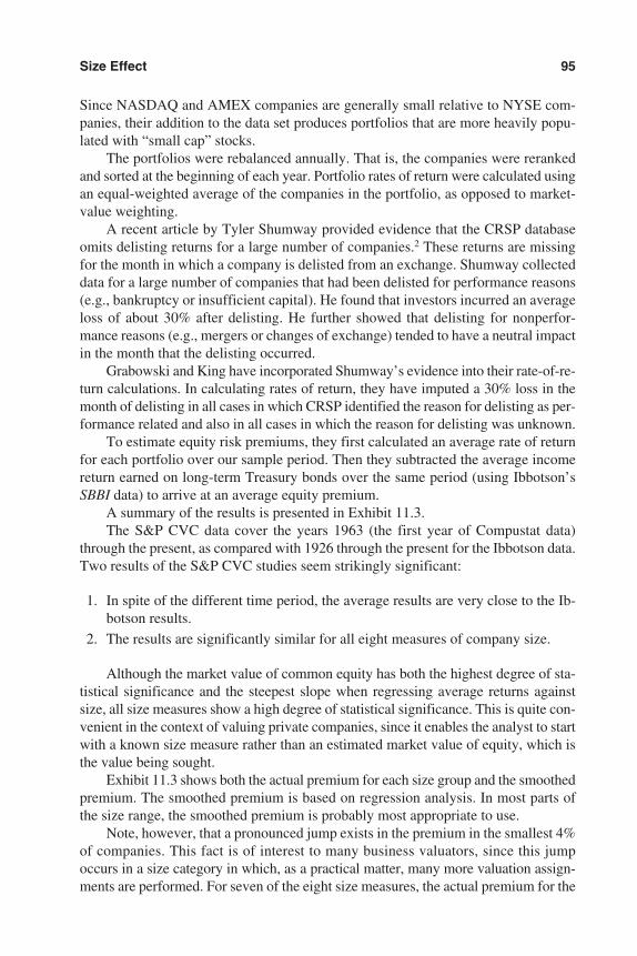
Since NASDAQ and AMEX companies are generally small relative to NYSE com-panies, their addition to the data set produces portfolios that are more heavily popu-lated with “small cap” stocks.
The portfolios were rebalanced annually. That is, the companies were rerankedand sorted at the beginning of each year. Portfolio rates of return were calculated usingan equal-weighted average of the companies in the portfolio, as opposed to market-value weighting.
A recent article by Tyler Shumway provided evidence that the CRSP databaseomits delisting returns for a large number of companies.2 These returns are missingfor the month in which a company is delisted from an exchange. Shumway collecteddata for a large number of companies that had been delisted for performance reasons(e.g., bankruptcy or insufficient capital). He found that investors incurred an averageloss of about 30% after delisting. He further showed that delisting for nonperfor-mance reasons (e.g., mergers or changes of exchange) tended to have a neutral impactin the month that the delisting occurred.
Grabowski and King have incorporated Shumway’s evidence into their rate-of-re-turn calculations. In calculating rates of return, they have imputed a 30% loss in themonth of delisting in all cases in which CRSP identified the reason for delisting as per-formance related and also in all cases in which the reason for delisting was unknown.
To estimate equity risk premiums, they first calculated an average rate of returnfor each portfolio over our sample period. Then they subtracted the average incomereturn earned on long-term Treasury bonds over the same period (using Ibbotson’sSBBI data) to arrive at an average equity premium.
A summary of the results is presented in Exhibit 11.3.The S&P CVC data cover the years 1963 (the first year of Compustat data)
through the present, as compared with 1926 through the present for the Ibbotson data.Two results of the S&P CVC studies seem strikingly significant:
1. In spite of the different time period, the average results are very close to the Ib-botson results.
2. The results are significantly similar for all eight measures of company size.
Although the market value of common equity has both the highest degree of sta-tistical significance and the steepest slope when regressing average returns againstsize, all size measures show a high degree of statistical significance. This is quite con-venient in the context of valuing private companies, since it enables the analyst to startwith a known size measure rather than an estimated market value of equity, which isthe value being sought.
Exhibit 11.3 shows both the actual premium for each size group and the smoothedpremium. The smoothed premium is based on regression analysis. In most parts ofthe size range, the smoothed premium is probably most appropriate to use.
Note, however, that a pronounced jump exists in the premium in the smallest 4%of companies. This fact is of interest to many business valuators, since this jumpoccurs in a size category in which, as a practical matter, many more valuation assign-ments are performed. For seven of the eight size measures, the actual premium for the
Size Effect 95
3953 P-11 8/29/02 2:23 PM Page 95
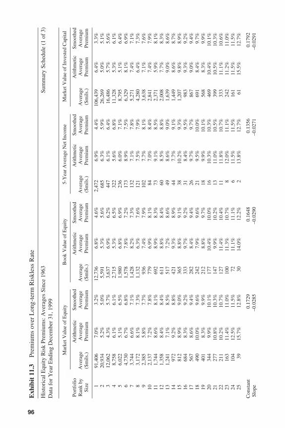
96
Exh
ibit
11.
3Pr
emiu
ms
over
Lon
g-te
rm R
iskl
ess
Rat
e
His
tori
cal E
quity
Ris
k Pr
emiu
ms:
Ave
rage
s Si
nce
1963
Sum
mar
y Sc
hedu
le (
1 of
3)
Dat
a fo
r Y
ear
End
ing
Dec
embe
r 31
, 199
9
Mar
ket V
alue
of
Equ
ityB
ook
Val
ue o
f E
quity
5-Y
ear
Ave
rage
Net
Inc
ome
Mar
ket V
alue
of
Inve
sted
Cap
ital
Port
folio
Ari
thm
etic
Smoo
thed
Ari
thm
etic
Smoo
thed
Ari
thm
etic
Smoo
thed
Ari
thm
etic
Smoo
thed
Ran
k by
Ave
rage
Ave
rage
Ave
rage
Ave
rage
Ave
rage
Ave
rage
Ave
rage
Ave
rage
Ave
rage
Ave
rage
Ave
rage
Ave
rage
Size
($m
ils.)
Prem
ium
Prem
ium
($m
ils.)
Prem
ium
Prem
ium
($m
ils.)
Prem
ium
Prem
ium
($m
ils.)
Prem
ium
Prem
ium
191
,406
7.0%
3.2%
12,7
366.
8%4.
6%2,
472
6.9%
4.4%
106,
439
6.4%
3.3%
220
,934
5.2%
5.0%
5,59
15.
3%5.
6%68
56.
3%5.
9%26
,269
5.0%
5.1%
312
,062
4.3%
5.7%
3,63
76.
9%6.
2%44
76.
1%6.
4%16
,486
5.7%
5.6%
48,
758
6.1%
6.1%
2,71
55.
3%6.
5%32
25.
6%6.
8%11
,328
5.3%
6.1%
56,
022
5.1%
6.5%
1,98
06.
8%6.
9%23
66.
0%7.
1%8,
795
5.1%
6.4%
64,
730
6.7%
6.8%
1,57
87.
8%7.
2%17
38.
9%7.
5%6,
329
8.1%
6.9%
73,
744
6.6%
7.1%
1,42
88.
2%7.
3%13
27.
1%7.
8%5,
271
7.4%
7.1%
83,
172
8.1%
7.3%
1,13
26.
3%7.
6%12
17.
5%7.
9%4,
280
6.4%
7.3%
92,
385
5.8%
7.7%
936
7.4%
7.9%
102
7.7%
8.1%
3,63
87.
1%7.
6%10
2,13
77.
2%7.
8%77
96.
9%8.
1%84
7.0%
8.4%
2,84
17.
4%7.
9%11
1,74
48.
6%8.
1%69
28.
9%8.
3%73
9.1%
8.5%
2,37
15.
9%8.
1%12
1,35
88.
4%8.
4%61
18.
8%8.
4%60
8.5%
8.8%
2,00
87.
7%8.
3%13
1,24
17.
1%8.
5%51
77.
2%8.
6%49
8.6%
9.0%
1,63
99.
0%8.
6%14
972
9.2%
8.8%
421
9.3%
8.9%
447.
7%9.
1%1,
449
8.6%
8.7%
1581
28.
9%9.
0%36
58.
8%9.
1%38
10.2
%9.
3%1,
207
9.8%
8.9%
1668
48.
3%9.
2%33
39.
7%9.
2%31
8.4%
9.5%
983
9.3%
9.2%
1756
78.
6%9.
4%28
28.
4%9.
4%26
9.7%
9.7%
867
9.0%
9.4%
1849
010
.0%
9.6%
242
7.9%
9.6%
219.
5%10
.0%
691
8.4%
9.7%
1940
18.
3%9.
9%21
28.
8%9.
7%18
9.9%
10.1
%56
88.
3%9.
9%20
344
9.9%
10.1
%17
710
.4%
10.0
%16
10.3
%10
.3%
469
10.4
%10
.1%
2127
710
.8%
10.3
%14
79.
9%10
.2%
1311
.0%
10.5
%39
910
.5%
10.3
%22
211
10.2
%10
.7%
127
11.4
%10
.4%
1111
.8%
10.7
%33
311
.1%
10.6
%23
163
11.4
%11
.0%
100
11.3
%10
.7%
812
.0%
11.1
%24
211
.2%
11.0
%24
104
12.5
%11
.5%
7211
.1%
11.1
%6
11.5
%11
.5%
161
11.5
%11
.5%
2539
15.7
%12
.8%
3014
.0%
12.2
%2
13.8
%12
.7%
6115
.5%
12.7
%
Con
stan
t0.
1729
0.16
480.
1356
0.17
92Sl
ope
–0.0
285
–0.0
290
–0.0
271
–0.0
291
3953 P-11 8/29/02 2:23 PM Page 96
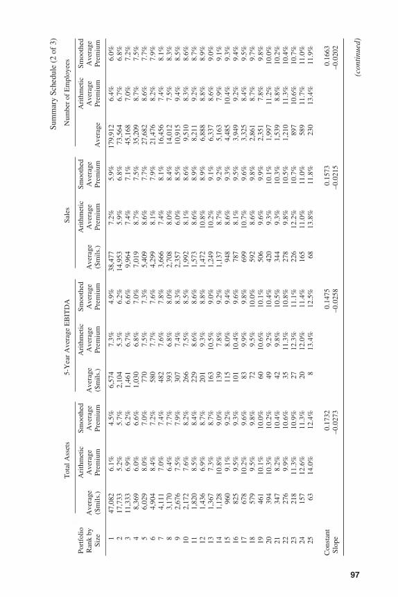
97
Tot
al A
sset
s5-
Yea
r A
vera
ge E
BIT
DA
Sale
sN
umbe
r of
Em
ploy
ees
Port
folio
Ari
thm
etic
Smoo
thed
Ari
thm
etic
Smoo
thed
Ari
thm
etic
Smoo
thed
Ari
thm
etic
Smoo
thed
Ran
k by
Ave
rage
Ave
rage
Ave
rage
Ave
rage
Ave
rage
Ave
rage
Ave
rage
Ave
rage
Ave
rage
Ave
rage
Ave
rage
Size
($m
ils.)
Prem
ium
Prem
ium
($m
ils.)
Prem
ium
Prem
ium
($m
ils.)
Prem
ium
Prem
ium
Ave
rage
Prem
ium
Prem
ium
147
,082
6.1%
4.5%
6,57
47.
3%4.
9%38
,477
7.2%
5.9%
179,
912
6.4%
6.0%
217
,733
5.2%
5.7%
2,10
45.
3%6.
2%14
,953
5.9%
6.8%
73,5
646.
7%6.
8%3
11,3
336.
9%6.
2%1,
461
6.7%
6.6%
9,96
47.
4%7.
1%45
,168
7.0%
7.2%
48,
369
6.0%
6.6%
1,03
06.
8%7.
0%7,
019
8.7%
7.5%
35,2
098.
7%7.
5%5
6,02
98.
0%7.
0%77
07.
5%7.
3%5,
409
8.6%
7.7%
27,6
828.
6%7.
7%6
4,90
48.
4%7.
2%58
07.
7%7.
6%4,
299
8.1%
7.9%
21,4
768.
2%7.
9%7
4,11
17.
0%7.
4%48
27.
6%7.
8%3,
666
7.4%
8.1%
16,4
567.
4%8.
1%8
3,17
06.
4%7.
7%39
36.
8%8.
0%2,
708
8.0%
8.4%
14,0
127.
5%8.
3%9
2,67
67.
5%7.
9%30
77.
4%8.
3%2,
357
6.0%
8.5%
10,9
159.
4%8.
5%10
2,17
27.
6%8.
2%26
67.
5%8.
5%1,
992
8.1%
8.6%
9,51
08.
3%8.
6%11
1,82
08.
5%8.
4%22
98.
6%8.
6%1,
573
8.6%
8.9%
8,21
19.
2%8.
7%12
1,43
66.
9%8.
7%20
19.
3%8.
8%1,
472
10.8
%8.
9%6,
888
8.8%
8.9%
131,
367
7.3%
8.7%
163
10.5
%9.
0%1,
249
10.2
%9.
1%6,
337
8.6%
9.0%
141,
128
10.8
%9.
0%13
97.
8%9.
2%1,
137
8.7%
9.2%
5,16
37.
9%9.
1%15
960
9.1%
9.2%
115
8.0%
9.4%
948
8.6%
9.3%
4,48
510
.4%
9.3%
1682
59.
5%9.
3%10
110
.4%
9.6%
787
8.1%
9.5%
3,94
99.
2%9.
4%17
678
10.2
%9.
6%83
9.9%
9.8%
699
10.7
%9.
6%3,
325
8.4%
9.5%
1857
99.
5%9.
8%72
9.5%
10.0
%59
28.
6%9.
8%2,
861
8.7%
9.7%
1946
110
.1%
10.0
%60
10.6
%10
.1%
506
9.6%
9.9%
2,35
17.
8%9.
8%20
394
10.3
%10
.2%
499.
2%10
.4%
420
9.3%
10.1
%1,
997
11.2
%10
.0%
2134
78.
2%10
.4%
429.
8%10
.5%
344
9.3%
10.3
%1,
539
8.8%
10.2
%22
276
9.9%
10.6
%35
11.3
%10
.8%
278
9.8%
10.5
%1,
210
11.3
%10
.4%
2321
811
.3%
10.9
%27
12.3
%11
.1%
226
12.2
%10
.7%
897
10.6
%10
.7%
2415
712
.6%
11.3
%20
12.0
%11
.4%
165
11.0
%11
.0%
589
11.7
%11
.0%
2563
14.0
%12
.4%
813
.4%
12.5
%68
13.8
%11
.8%
230
13.4
%11
.9%
Con
stan
t0.
1732
0.14
750.
1573
0.16
63Sl
ope
–0.0
273
–0.0
258
–0.0
215
–0.0
202
(con
tinu
ed)
Sum
mar
y Sc
hedu
le (
2 of
3)
3953 P-11 8/29/02 2:23 PM Page 97
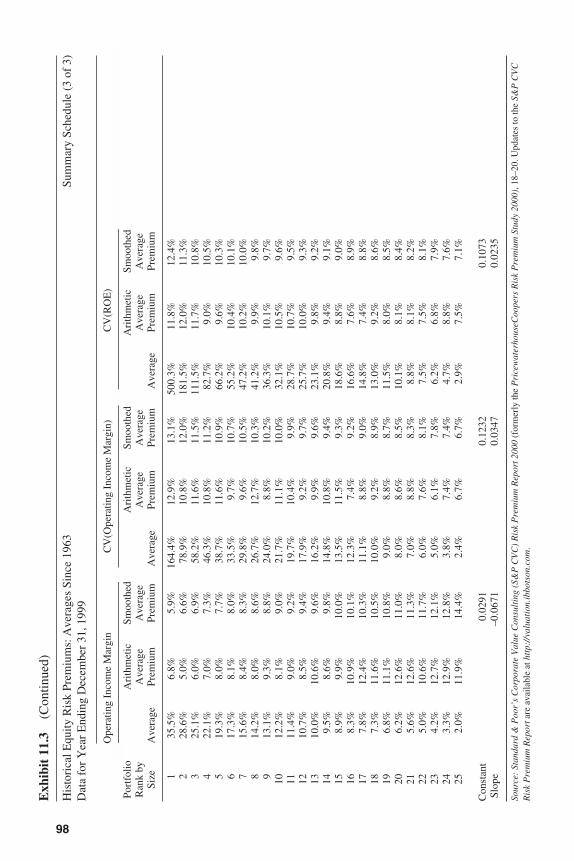
98
Exh
ibit
11.
3(C
ontin
ued)
His
tori
cal E
quity
Ris
k Pr
emiu
ms:
Ave
rage
s Si
nce
1963
Sum
mar
y Sc
hedu
le (
3 of
3)
Dat
a fo
r Y
ear
End
ing
Dec
embe
r 31
, 199
9
Ope
ratin
g In
com
e M
argi
nC
V(O
pera
ting
Inco
me
Mar
gin)
CV
(RO
E)
Port
folio
Ari
thm
etic
Smoo
thed
Ari
thm
etic
Smoo
thed
Ari
thm
etic
Smoo
thed
Ran
k by
Ave
rage
Ave
rage
Ave
rage
Ave
rage
Ave
rage
Ave
rage
Size
Ave
rage
Prem
ium
Prem
ium
Ave
rage
Prem
ium
Prem
ium
Ave
rage
Prem
ium
Prem
ium
135
.5%
6.8%
5.9%
164.
4%12
.9%
13.1
%50
0.3%
11.8
%12
.4%
228
.6%
5.0%
6.6%
78.9
%10
.8%
12.0
%18
1.5%
12.0
%11
.3%
325
.1%
6.0%
6.9%
58.2
%11
.6%
11.5
%11
1.5%
11.7
%10
.8%
422
.1%
7.0%
7.3%
46.3
%10
.8%
11.2
%82
.7%
9.0%
10.5
%5
19.3
%8.
0%7.
7%38
.7%
11.6
%10
.9%
66.2
%9.
6%10
.3%
617
.3%
8.1%
8.0%
33.5
%9.
7%10
.7%
55.2
%10
.4%
10.1
%7
15.6
%8.
4%8.
3%29
.8%
9.6%
10.5
%47
.2%
10.2
%10
.0%
814
.2%
8.0%
8.6%
26.7
%12
.7%
10.3
%41
.2%
9.9%
9.8%
913
.1%
9.3%
8.8%
24.0
%8.
8%10
.2%
36.3
%10
.1%
9.7%
1012
.2%
8.1%
9.0%
21.7
%11
.1%
10.0
%32
.1%
10.5
%9.
6%11
11.4
%9.
0%9.
2%19
.7%
10.4
%9.
9%28
.7%
10.7
%9.
5%12
10.7
%8.
5%9.
4%17
.9%
9.2%
9.7%
25.7
%10
.0%
9.3%
1310
.0%
10.6
%9.
6%16
.2%
9.9%
9.6%
23.1
%9.
8%9.
2%14
9.5%
8.6%
9.8%
14.8
%10
.8%
9.4%
20.8
%9.
4%9.
1%15
8.9%
9.9%
10.0
%13
.5%
11.5
%9.
3%18
.6%
8.8%
9.0%
168.
3%10
.9%
10.1
%12
.3%
7.4%
9.2%
16.6
%7.
6%8.
9%17
7.8%
12.4
%10
.3%
11.1
%8.
8%9.
0%14
.8%
7.4%
8.8%
187.
3%11
.6%
10.5
%10
.0%
9.2%
8.9%
13.0
%9.
2%8.
6%19
6.8%
11.1
%10
.8%
9.0%
8.8%
8.7%
11.5
%8.
0%8.
5%20
6.2%
12.6
%11
.0%
8.0%
8.6%
8.5%
10.1
%8.
1%8.
4%21
5.6%
12.6
%11
.3%
7.0%
8.8%
8.3%
8.8%
8.1%
8.2%
225.
0%10
.6%
11.7
%6.
0%7.
6%8.
1%7.
5%7.
5%8.
1%23
4.2%
12.7
%12
.1%
5.0%
6.1%
7.8%
6.2%
6.8%
7.9%
243.
3%12
.9%
12.8
%3.
8%7.
4%7.
4%4.
7%8.
8%7.
6%25
2.0%
11.9
%14
.4%
2.4%
6.7%
6.7%
2.9%
7.5%
7.1%
Con
stan
t0.
0291
0.12
320.
1073
Slop
e–0
.067
10.
0347
0.02
35
Sour
ce:
Stan
dard
& P
oor’
s C
orpo
rate
Val
ue C
onsu
ltin
g (S
&P
CV
C)
Ris
k P
rem
ium
Rep
ort 2
000
(for
mer
ly th
e P
rice
wat
erho
useC
oope
rs R
isk
Pre
miu
m S
tudy
200
0), 1
8–20
. Upd
ates
to th
e S&
P C
VC
Ris
k P
rem
ium
Rep
orta
re a
vaila
ble
at h
ttp:
//va
luat
ion.
ibbo
tson
.com
.
3953 P-11 8/29/02 2:23 PM Page 98
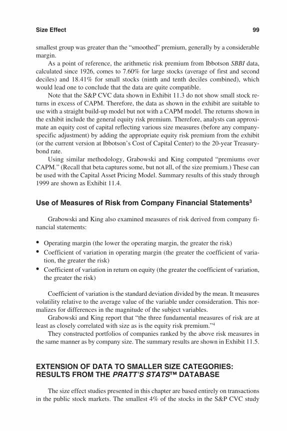
smallest group was greater than the “smoothed” premium, generally by a considerablemargin.
As a point of reference, the arithmetic risk premium from Ibbotson SBBI data,calculated since 1926, comes to 7.60% for large stocks (average of first and seconddeciles) and 18.41% for small stocks (ninth and tenth deciles combined), whichwould lead one to conclude that the data are quite compatible.
Note that the S&P CVC data shown in Exhibit 11.3 do not show small stock re-turns in excess of CAPM. Therefore, the data as shown in the exhibit are suitable touse with a straight build-up model but not with a CAPM model. The returns shown inthe exhibit include the general equity risk premium. Therefore, analysts can approxi-mate an equity cost of capital reflecting various size measures (before any company-specific adjustment) by adding the appropriate equity risk premium from the exhibit(or the current version at Ibbotson’s Cost of Capital Center) to the 20-year Treasury-bond rate.
Using similar methodology, Grabowski and King computed “premiums overCAPM.” (Recall that beta captures some, but not all, of the size premium.) These canbe used with the Capital Asset Pricing Model. Summary results of this study through1999 are shown as Exhibit 11.4.
Use of Measures of Risk from Company Financial Statements3
Grabowski and King also examined measures of risk derived from company fi-nancial statements:
• Operating margin (the lower the operating margin, the greater the risk)
• Coefficient of variation in operating margin (the greater the coefficient of varia-tion, the greater the risk)
• Coefficient of variation in return on equity (the greater the coefficient of variation,the greater the risk)
Coefficient of variation is the standard deviation divided by the mean. It measuresvolatility relative to the average value of the variable under consideration. This nor-malizes for differences in the magnitude of the subject variables.
Grabowski and King report that “the three fundamental measures of risk are atleast as closely correlated with size as is the equity risk premium.”4
They constructed portfolios of companies ranked by the above risk measures inthe same manner as by company size. The summary results are shown in Exhibit 11.5.
EXTENSION OF DATA TO SMALLER SIZE CATEGORIES:RESULTS FROM THE PRATT’S STATS™ DATABASE
The size effect studies presented in this chapter are based entirely on transactionsin the public stock markets. The smallest 4% of the stocks in the S&P CVC study
Size Effect 99
3953 P-11 8/29/02 2:23 PM Page 99
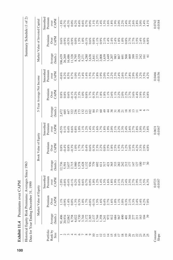
100
Exh
ibit
11.
4Pr
emiu
ms
over
CA
PM
His
tori
cal E
quity
Ris
k Pr
emiu
ms:
Ave
rage
s Si
nce
1963
Sum
mar
y Sc
hedu
le (
1 of
2)
Dat
a fo
r Y
ear
End
ing
Dec
embe
r 31
, 199
9
Mar
ket V
alue
of
Equ
ityB
ook
Val
ue o
f E
quity
5-Y
ear
Ave
rage
Net
Inc
ome
Mar
ket V
alue
of
Inve
sted
Cap
ital
Smoo
thed
Smoo
thed
Smoo
thed
Smoo
thed
Port
folio
Prem
ium
Prem
ium
Prem
ium
Prem
ium
Prem
ium
Prem
ium
Prem
ium
Prem
ium
Ran
k by
Ave
rage
Ove
rov
erA
vera
geO
ver
over
Ave
rage
Ove
rov
erA
vera
geO
ver
over
Size
($m
ils.)
CA
PMC
APM
($m
ils.)
CA
PMC
APM
($m
ils.)
CA
PMC
APM
($m
ils.)
CA
PMC
APM
191
,406
1.1%
–2.0
%12
,736
0.8%
–0.5
%2,
472
0.8%
–0.6
%10
6,43
90.
6%–1
.8%
220
,934
–0.9
%–0
.8%
5,59
1–0
.4%
0.1%
685
0.8%
0.2%
26,2
69–0
.9%
–0.7
%3
12,0
62–1
.4%
–0.4
%3,
637
0.8%
0.4%
447
0.6%
0.5%
16,4
86–0
.5%
–0.3
%4
8,75
80.
0%–0
.1%
2,71
5–0
.3%
0.6%
322
–0.1
%0.
7%11
,328
–0.9
%0.
0%5
6,02
2–1
.3%
0.2%
1,98
01.
0%0.
8%23
6–0
.2%
1.0%
8,79
50.
0%0.
2%6
4,73
00.
3%0.
4%1,
578
1.7%
1.0%
173
2.3%
1.2%
6,32
91.
5%0.
4%7
3,74
41.
0%0.
6%1,
428
1.7%
1.1%
132
1.0%
1.4%
5,27
11.
0%0.
6%8
3,17
21.
7%0.
7%1,
132
0.4%
1.2%
121
0.8%
1.4%
4,28
0–0
.1%
0.7%
92,
385
–0.8
%0.
9%93
60.
6%1.
4%10
21.
7%1.
5%3,
638
0.6%
0.9%
102,
137
–0.1
%1.
0%77
90.
3%1.
5%84
0.3%
1.7%
2,84
10.
8%1.
1%11
1,74
41.
5%1.
2%69
22.
3%1.
6%73
2.7%
1.8%
2,37
1–1
.1%
1.2%
121,
358
1.6%
1.4%
611
2.2%
1.7%
601.
8%1.
9%2,
008
0.9%
1.4%
131,
241
0.4%
1.5%
517
0.8%
1.8%
491.
8%2.
0%1,
639
2.1%
1.5%
1497
22.
7%1.
6%42
12.
5%1.
9%44
1.1%
2.1%
1,44
91.
4%1.
6%15
812
1.6%
1.8%
365
1.8%
2.0%
382.
6%2.
2%1,
207
2.4%
1.8%
1668
41.
0%1.
9%33
32.
5%2.
1%31
1.1%
2.3%
983
2.4%
1.9%
1756
71.
1%2.
1%28
21.
5%2.
2%26
2.2%
2.4%
867
1.8%
2.0%
1849
03.
0%2.
2%24
21.
2%2.
3%21
2.0%
2.6%
691
1.0%
2.2%
1940
10.
3%2.
4%21
21.
2%2.
4%18
2.2%
2.7%
568
0.8%
2.4%
2034
42.
1%2.
5%17
73.
6%2.
6%16
2.7%
2.8%
469
2.7%
2.5%
2127
73.
3%2.
7%14
72.
3%2.
7%13
3.6%
2.9%
399
2.7%
2.6%
2221
12.
4%2.
9%12
74.
2%2.
8%11
4.4%
3.0%
333
3.5%
2.8%
2316
33.
4%3.
1%10
03.
3%3.
0%8
3.9%
3.2%
242
2.4%
3.0%
2410
44.
2%3.
5%72
2.9%
3.2%
63.
5%3.
5%16
13.
6%3.
4%25
397.
0%4.
3%30
4.8%
3.8%
24.
8%4.
2%61
6.8%
4.1%
Con
stan
t0.
0723
0.06
310.
0466
0.07
42Sl
ope
–0.0
187
–0.0
167
–0.0
156
–0.0
184
3953 P-11 8/29/02 2:23 PM Page 100
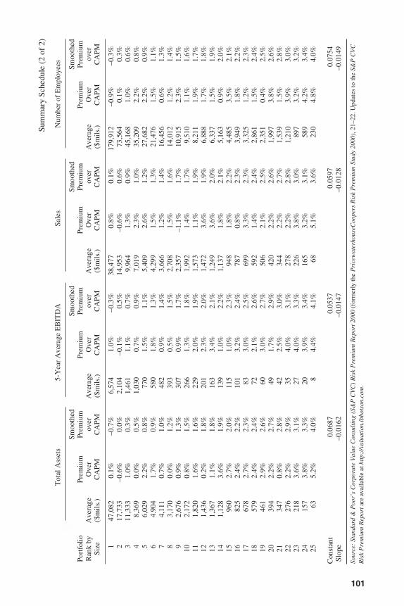
101
Tot
al A
sset
s5-
Yea
r A
vera
ge E
BIT
DA
Sale
sN
umbe
r of
Em
ploy
ees
Smoo
thed
Smoo
thed
Smoo
thed
Smoo
thed
Port
folio
Prem
ium
Prem
ium
Prem
ium
Prem
ium
Prem
ium
Prem
ium
Prem
ium
Prem
ium
Ran
k by
Ave
rage
Ove
rov
erA
vera
geO
ver
over
Ave
rage
Ove
rov
erA
vera
geO
ver
over
Size
($m
ils.)
CA
PMC
APM
($m
ils.)
CA
PMC
APM
($m
ils.)
CA
PMC
APM
($m
ils.)
CA
PMC
APM
147
,082
0.1%
–0.7
%6,
574
1.0%
–0.3
%38
,477
0.8%
0.1%
179,
912
–0.9
%–0
.3%
217
,733
–0.6
%0.
0%2,
104
–0.1
%0.
5%14
,953
–0.6
%0.
6%73
,564
0.1%
0.3%
311
,333
1.0%
0.3%
1,46
11.
1%0.
7%9,
964
1.3%
0.9%
45,1
681.
0%0.
6%4
8,36
90.
0%0.
5%1,
030
0.7%
0.9%
7,01
92.
3%1.
0%35
,209
2.2%
0.8%
56,
029
2.2%
0.8%
770
1.5%
1.1%
5,40
92.
6%1.
2%27
,682
2.2%
0.9%
64.
904
1.7%
0.9%
580
1.8%
1.3%
4,29
91.
5%1.
3%21
,476
1.5%
1.1%
74,
111
0.7%
1.0%
482
0.9%
1.4%
3,66
61.
2%1.
4%16
,456
0.6%
1.3%
83,
170
0.0%
1.2%
393
0.5%
1.5%
2,70
81.
5%1.
6%14
,012
1.2%
1.4%
92,
676
0.9%
1.3%
307
0.9%
1.7%
2,35
7–1
.1%
1.7%
10,9
152.
3%1.
5%10
2,17
20.
8%1.
5%26
61.
3%1.
8%1,
992
1.4%
1.7%
9,51
01.
1%1.
6%11
1,82
01.
6%1.
6%22
92.
0%1.
9%1,
573
1.1%
1.9%
8,21
11.
9%1.
7%12
1,43
60.
2%1.
8%20
12.
3%2.
0%1,
472
3.6%
1.9%
6,88
81.
7%1.
8%13
1,36
71.
1%1.
8%16
33.
4%2.
1%1,
249
3.6%
2.0%
6,33
71.
5%1.
9%14
1,12
83.
6%1.
9%13
91.
0%2.
2%1,
137
1.8%
2.1%
5,16
30.
9%2.
0%15
960
2.7%
2.0%
115
1.0%
2.3%
948
1.8%
2.2%
4,48
53.
5%2.
1%16
825
2.4%
2.2%
101
3.2%
2.4%
787
0.8%
2.3%
3,94
91.
8%2.
2%17
678
2.7%
2.3%
833.
0%2.
5%69
93.
3%2.
3%3,
325
1.2%
2.3%
1857
92.
4%2.
4%72
2.1%
2.6%
592
1.4%
2.4%
2,86
11.
5%2.
4%19
461
2.9%
2.6%
603.
0%2.
7%50
62.
1%2.
5%2,
351
0.4%
2.5%
2039
42.
2%2.
7%49
1.7%
2.9%
420
2.2%
2.6%
1,99
73.
8%2.
6%21
347
0.8%
2.8%
422.
5%3.
0%34
42.
2%2.
7%1,
539
1.5%
2.8%
2227
62.
2%2.
9%35
4.0%
3.1%
278
2.2%
2.8%
1,21
03.
9%3.
0%23
218
3.6%
3.1%
274.
0%3.
3%22
63.
8%3.
0%89
73.
2%3.
2%24
157
3.8%
3.3%
203.
9%3.
4%16
53.
2%3.
1%58
94.
2%3.
4%25
635.
2%4.
0%8
4.4%
4.1%
685.
1%3.
6%23
04.
8%4.
0%
Con
stan
t0.
0687
0.05
370.
0597
0.07
54Sl
ope
–0.0
162
–0.0
147
–0.0
128
–0.0
149
Sour
ce:
Stan
dard
& P
oor’
s C
orpo
rate
Val
ue C
onsu
ltin
g (S
&P
CV
C)
Ris
k P
rem
ium
Rep
ort 2
000
(for
mer
ly th
e P
rice
wat
erho
useC
oope
rs R
isk
Pre
miu
m S
tudy
200
0), 2
1–22
. Upd
ates
to th
e S&
P C
VC
Ris
k P
rem
ium
Rep
orta
re a
vaila
ble
at h
ttp:
//va
luat
ion.
ibbo
tson
.com
.
Sum
mar
y Sc
hedu
le (
2 of
2)
3953 P-11 8/29/02 2:23 PM Page 101
102
Exh
ibit
11.
5C
ompa
nies
Ran
ked
by M
easu
re o
f R
isk
Com
pani
es R
anke
d by
Ope
ratin
g M
argi
nH
isto
rica
l Equ
ity R
isk
Prem
ium
: Ave
rage
Sin
ce 1
963
Dat
a fo
r Y
ear
End
ing
Dec
embe
r 31
, 199
9Sm
ooth
edPo
rtfo
lioM
edia
nL
og o
fN
umbe
rB
eta
Stan
dard
Geo
met
ric
Ari
thm
etic
Ari
thm
etic
Ave
rage
Ave
rage
Ran
kO
pera
ting
Med
ian
as o
fA
nnua
lD
evia
tion
Ave
rage
Ave
rage
Equ
ity R
isk
Equ
ity
Ris
kD
ebt/
by S
ize
Mar
gin
Op
Mar
gin
1999
Sinc
e ‘6
3of
Ret
urns
Ret
urn
Ret
urn
Prem
ium
Pre
miu
mM
VIC
135
.5%
–0.4
584
0.88
17.5
3%13
.02%
14.3
0%6.
80%
5.93
%32
.30%
228
.6%
–0.5
469
0.82
14.9
3%11
.48%
12.4
7%4.
97%
6.56
%36
.74%
325
.1%
–0.6
058
0.88
15.3
3%12
.37%
13.4
6%5.
96%
6.94
%33
.44%
422
.1%
–0.6
676
0.97
17.2
2%13
.21%
14.5
4%7.
04%
7.31
%26
.68%
519
.3%
–0.7
170
1.01
18.3
3%14
.00%
15.4
7%7.
97%
7.70
%22
.57%
617
.3%
–0.7
683
1.03
18.6
3%14
.04%
15.5
7%8.
07%
8.03
%19
.39%
715
.6%
–0.8
173
1.07
19.7
1%14
.25%
15.9
1%8.
41%
8.32
%19
.40%
814
.2%
–0.8
572
1.06
19.8
8%13
.73%
15.5
3%8.
03%
8.59
%20
.25%
913
.1%
–0.8
866
1.15
20.9
2%15
.00%
16.8
2%9.
32%
8.83
%21
.34%
1012
.2%
–0.9
161
1.13
20.9
7%13
.66%
15.5
7%8.
07%
9.04
%21
.87%
1111
.4%
–0.9
471
1.23
23.2
4%14
.15%
16.4
5%8.
95%
9.23
%22
.89%
1210
.7%
–0.9
769
1.18
23.4
5%13
.63%
15.9
6%8.
46%
9.42
%23
.44%
1310
.0%
–1.0
078
1.20
23.6
2%15
.69%
18.1
0%10
.60%
9.61
%24
.00%
149.
5%–1
.02
891.
1822
.82%
13.8
8%16
.12%
8.62
%9.
78%
23.9
2%15
8.9%
–1.0
580
1.20
23.7
0%15
.04%
17.4
4%9.
94%
9.96
%25
.95%
168.
3%–1
.08
851.
2324
.51%
15.7
2%18
.36%
10.8
6%10
.15%
27.5
9%17
7.8%
–1.1
198
1.23
25.1
1%17
.32%
19.9
1%12
.41%
10.3
4%28
.30%
187.
3%–1
.14
921.
3227
.08%
16.1
1%19
.14%
11.6
4%10
.54%
28.8
8%19
6.8%
–1.1
797
1.15
23.9
8%16
.13%
18.5
6%11
.06%
10.7
6%29
.97%
206.
2%–1
.21
981.
2827
.28%
17.0
4%20
.09%
12.5
9%11
.00%
32.2
4%21
5.6%
–1.2
510
11.
2626
.21%
17.2
3%20
.05%
12.5
5%11
.29%
32.2
7%22
5.0%
–1.3
084
1.27
26.3
3%15
.14%
18.0
8%10
.58%
11.6
6%32
.81%
234.
2%–1
.37
135
1.19
26.0
2%17
.41%
20.2
0%12
.70%
12.1
4%34
.87%
243.
3%–1
.48
103
1.29
29.7
7%16
.80%
20.3
5%12
.85%
12.8
3%34
.80%
252.
0%–1
.71
169
1.27
28.8
6%16
.08%
19.3
8%11
.88%
14.3
8%34
.19%
Hig
h fi
nanc
ial r
isk
644
1.50
37.2
7%14
.97%
20.2
4%12
.74%
49.6
8%
Lar
ge S
tock
s (I
bbot
son
SBB
I da
ta)
12.8
1%13
.92%
6.42
%Sm
all S
tock
s (I
bbot
son
SBB
I da
ta)
15.3
6%18
.09%
10.5
9%
Lon
g-te
rm T
reas
ury
Inco
me
(Ibb
osto
n SB
BI
data
)7.
48%
7.50
%
Equ
ity R
isk
Prem
ium
Stu
dy: D
ata
thro
ugh
Dec
embe
r 31
, 199
9
Dat
a Sm
ooth
ing
with
Reg
ress
ion
Ana
lysi
sD
epen
dent
Var
iabl
e: A
vera
ge P
rem
ium
Inde
pend
ent V
aria
ble:
Log
of
Med
ian
Ope
ratin
g M
argi
n
Reg
ress
ion
Out
put:
Con
stan
t2.
907%
Std
Err
of
Y E
st1.
086%
R S
quar
ed78
%N
o. o
f O
bser
vatio
ns25
Deg
rees
of
Free
dom
23
X C
oeff
icie
nt(s
)–6
.714
%St
d E
rr o
f C
oef.
0.74
1%t-
Stat
istic
–9.0
6
Smoo
thed
Pre
miu
m =
2.9
07%
– 6
.714
% *
Log
(Ope
rati
ng M
argi
n)
20%
18%
16%
14%
12%
10% 8% 6% 4% 2% 0%
-1.8
-1.6
-1.4
-1.2
-1.0
Med
ian O
perat
ing M
argin
Smoo
thed P
remium
vs. U
nadju
sted A
verag
e
Equity Premium
-0.8
-0.6
-0.4
-0.2
-0.0
3953 P-11 8/29/02 2:23 PM Page 102
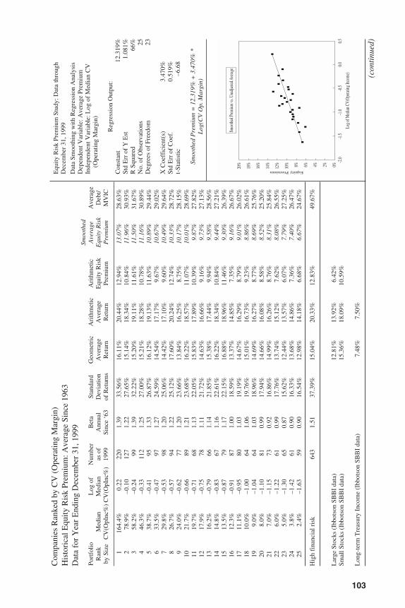
103
Com
pani
es R
anke
d by
CV
(O
pera
ting
Mar
gin)
His
tori
cal E
quity
Ris
k Pr
emiu
m: A
vera
ge S
ince
196
3D
ata
for
Yea
r E
ndin
g D
ecem
ber
31, 1
999
Smoo
thed
Port
folio
Log
of
Num
ber
Bet
aSt
anda
rdG
eom
etri
cA
rith
met
icA
rith
met
icA
vera
geA
vera
geR
ank
Med
ian
Med
ian
as o
fA
nnua
lD
evia
tion
Ave
rage
Ave
rage
Equ
ity R
isk
Equ
ity
Ris
kD
ebt/
by S
ize
CV
(OpI
nc%
) C
V(O
pInc
%)
1999
Sinc
e ‘6
3of
Ret
urns
Ret
urn
Ret
urn
Prem
ium
Pre
miu
mM
VIC
116
4.4%
0.22
220
1.39
33.5
6%16
.11%
20.4
4%12
.94%
13.0
7%28
.63%
278
.9%
–0.1
012
71.
2227
.65%
15.1
4%18
.34%
10.8
4%11
.96%
30.9
3%3
58.2
%–0
.24
991.
3932
.22%
15.2
0%19
.11%
11.6
1%11
.50%
31.6
7%4
46.3
%–0
.33
112
1.25
27.0
0%15
.21%
18.2
8%10
.78%
11.1
6%30
.89%
538
.7%
–0.4
195
1.33
26.8
7%16
.12%
19.1
3%11
.63%
10.8
9%29
.44%
633
.5%
–0.4
797
1.27
24.5
9%14
.54%
17.1
7%9.
67%
10.6
7%29
.02%
729
.8%
–0.5
398
1.20
25.0
6%14
.42%
17.1
0%9.
60%
10.4
9%29
.64%
826
.7%
–0.5
794
1.22
25.1
2%17
.60%
20.2
4%12
.74%
10.3
3%28
.72%
924
.0%
–0.6
277
1.20
23.6
6%13
.84%
16.2
5%8.
75%
10.1
7%28
.15%
1021
.7%
–0.6
689
1.21
23.6
8%16
.22%
18.5
7%11
.07%
10.0
1%28
.69%
1119
.7%
–0.7
168
1.13
22.0
5%15
.83%
17.8
9%10
.39%
9.87
%27
.82%
1217
.9%
–0.7
578
1.11
21.7
2%14
.63%
16.6
6%9.
16%
9.73
%27
.13%
1316
.2%
–0.7
966
1.14
21.8
5%15
.38%
17.4
4%9.
94%
9.58
%28
.56%
1414
.8%
–0.8
367
1.16
22.6
1%16
.22%
18.3
4%10
.84%
9.44
%27
.21%
1513
.5%
–0.8
779
1.17
22.1
5%16
.88%
18.9
6%11
.46%
9.30
%26
.39%
1612
.3%
–0.9
187
1.00
18.5
9%13
.37%
14.8
5%7.
35%
9.16
%26
.67%
1711
.1%
–0.9
580
1.03
19.1
9%14
.67%
16.2
9%8.
79%
9.01
%26
.02%
1810
.0%
–1.0
064
1.06
19.7
6%15
.01%
16.7
3%9.
23%
8.86
%26
.61%
199.
0%–1
.04
641.
0318
.96%
14.6
9%16
.27%
8.77
%8.
69%
25.7
6%20
8.0%
–1.1
081
0.99
17.9
4%14
.66%
16.0
8%8.
58%
8.52
%25
.20%
217.
0%–1
.15
730.
9216
.86%
14.9
9%16
.26%
8.76
%8.
31%
25.8
4%22
6.0%
–1.2
261
0.99
17.7
6%13
.74%
15.1
2%7.
62%
8.08
%26
.55%
235.
0%–1
.30
650.
8715
.62%
12.4
4%13
.57%
6.07
%7.
79%
27.2
5%24
3.8%
–1.4
261
0.90
16.3
3%13
.68%
14.8
6%7.
36%
7.40
%26
.47%
252.
4%–1
.63
590.
9016
.54%
12.9
8%14
.18%
6.68
%6.
67%
24.6
7%
Hig
h fi
nanc
ial r
isk
643
1.51
37.3
9%15
.04%
20.3
3%12
.83%
49.6
7%
Lar
ge S
tock
s (I
bbot
son
SBB
I da
ta)
12.8
1%13
.92%
6.42
%Sm
all S
tock
s (I
bbot
son
SBB
I da
ta)
15.3
6%18
.09%
10.5
9%
Lon
g-te
rm T
reas
ury
Inco
me
(Ibb
otso
n SB
BI
data
)7.
48%
7.50
%
Equ
ity R
isk
Prem
ium
Stu
dy: D
ata
thro
ugh
Dec
embe
r 31
, 199
9
Dat
a Sm
ooth
ing
with
Reg
ress
ion
Ana
lysi
sD
epen
dent
Var
iabl
e: A
vera
ge P
rem
ium
Inde
pend
ent V
aria
ble:
Log
of
Med
ian
CV
(O
pera
ting
Mar
gin)
Reg
ress
ion
Out
put:
Con
stan
t12
.319
%St
d E
rr o
f Y
Est
1.08
1%R
Squ
ared
66%
No.
of
Obs
erva
tions
25D
egre
es o
f Fr
eedo
m23
X C
oeff
icie
nt(s
)3.
470%
Std
Err
of
Coe
f.0.
519%
t-St
atis
tic–6
.68
Smoo
thed
Pre
miu
m =
12.
319%
+ 3
.470
% *
Log
(CV
Op.
Mar
gin)
20%
18%
16%
14%
12%
10% 8% 6% 4% 2% 0%
-2.0
-1.5
-1.0
Log o
f Med
ian C
V(Op
eratin
g Inc
ome)
Smoo
thed P
remium
vs. U
nadju
sted A
verag
e
Equity Premium
-0.5
0.00.5
(con
tinu
ed)
3953 P-11 8/29/02 2:23 PM Page 103
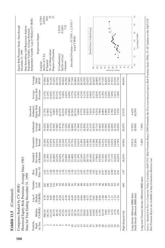
104
Exh
ibit
11.
5(C
ontin
ued)
Com
pani
es R
anke
d by
CV
(R
OE
)H
isto
rica
l Equ
ity R
isk
Prem
ium
: Ave
rage
Sin
ce 1
963
Dat
a fo
r Y
ear
End
ing
Dec
embe
r 31
, 199
9Sm
ooth
edPo
rtfo
lioL
og o
fN
umbe
rB
eta
Stan
dard
Geo
met
ric
Ari
thm
etic
Ari
thm
etic
Ave
rage
Ave
rage
Ran
kM
edia
nM
edia
nas
of
Ann
ual
Dev
iatio
nA
vera
geA
vera
geE
quity
Ris
kE
quit
y R
isk
Deb
t/by
Siz
eC
V(R
OE
)C
V(R
OE
)19
99Si
nce
‘63
of R
etur
nsR
etur
nR
etur
nPr
emiu
mP
rem
ium
MV
IC
150
0.3%
0.70
102
1.43
32.7
0%15
.10%
19.2
5%11
.75%
12.3
7%37
.98%
218
1.5%
0.26
106
1.37
31.3
9%15
.45%
19.4
6%11
.96%
11.3
4%35
.60%
311
1.5%
0.05
122
1.28
27.9
1%15
.93%
19.1
7%11
.67%
10.8
4%34
.12%
482
.7%
–0.0
811
61.
3026
.88%
13.4
5%16
.50%
9.00
%10
.53%
33.4
2%5
66.2
%–0
.18
991.
2424
.22%
14.5
1%17
.08%
9.58
%10
.31%
30.7
2%6
55.2
%–0
.26
921.
2225
.62%
15.1
0%17
.87%
10.3
7%10
.12%
30.4
3%7
47.2
%–0
.33
991.
1624
.17%
15.1
4%17
.73%
10.2
3%9.
96%
30.0
5%8
41.2
%–0
.38
891.
1322
.89%
15.1
7%17
.42%
9.92
%9.
82%
28.3
9%9
36.3
%–0
.44
891.
2023
.40%
15.2
1%17
.59%
10.0
9%9.
69%
27.8
6%10
32.1
%–0
.49
811.
1623
.40%
15.7
3%18
.00%
10.5
0%9.
57%
27.7
4%11
28.7
%–0
.54
781.
2123
.12%
15.9
3%18
.23%
10.7
3%9.
45%
26.9
0%12
25.7
%–0
.59
801.
1221
.35%
15.6
1%17
.49%
9.99
%9.
34%
26.2
6%13
23.1
%–0
.64
881.
0722
.18%
15.3
0%17
.27%
9.77
%9.
23%
26.3
2%14
20.8
%–0
.68
851.
0720
.91%
15.0
4%16
.95%
9.45
%9.
12%
26.3
9%15
18.6
%–0
.73
851.
1020
.71%
14.4
8%16
.31%
8.81
%9.
01%
25.6
2%16
16.6
%–0
.78
941.
0520
.16%
13.3
2%15
.11%
7.61
%8.
90%
26.1
1%17
14.8
%–0
.83
781.
0719
.87%
13.1
8%14
.91%
7.41
%8.
77%
26.8
1%18
13.0
%–0
.89
750.
9717
.96%
15.3
0%16
.71%
9.21
%8.
65%
26.0
8%19
11.5
%–0
.94
901.
0719
.29%
13.8
5%15
.46%
7.96
%8.
52%
26.7
3%20
10.1
%–1
.00
660.
9717
.34%
14.2
1%15
.58%
8.08
%8.
38%
27.7
2%21
8.8%
–1.0
680
0.95
18.5
6%14
.12%
15.5
8%8.
08%
8.24
%26
.65%
227.
5%–1
.13
690.
8716
.17%
13.9
3%15
.05%
7.55
%8.
08%
27.8
2%23
6.2%
–1.2
182
0.90
17.1
1%13
.03%
14.2
8%6.
78%
7.88
%27
.91%
244.
7%–1
.33
630.
9116
.83%
15.0
4%16
.32%
8.82
%7.
61%
25.5
3%25
2.9%
–1.5
456
0.91
16.8
3%13
.79%
15.0
3%7.
53%
7.09
%23
.73%
Hig
h fi
nanc
ial r
isk
640
1.47
36.6
3%14
.96%
20.0
7%12
.57%
49.6
4%
Lar
ge S
tock
s (I
bbot
son
SBB
I da
ta)
12.8
1%13
.92%
6.42
%Sm
all S
tock
s (I
bbot
son
SBB
I da
ta)
15.3
6%18
.09%
10.5
9%
Lon
g-te
rm T
reas
ury
Inco
me
(Ibb
otso
n SB
BI
data
)7.
48%
7.50
%
Sour
ce:
Stan
dard
& P
oor’
s C
orpo
rate
Val
ue C
onsu
ltin
g (S
&P
CV
C)
Ris
k P
rem
ium
Rep
ort 2
000
(for
mer
ly th
e P
rice
wat
erho
useC
oope
rs R
isk
Pre
miu
m S
tudy
200
0), 4
7–49
. Upd
ates
to th
e S&
P C
VC
Ris
k P
rem
ium
Rep
orta
re a
vaila
ble
at h
ttp:
//va
luat
ion.
ibbo
tson
.com
.
Equ
ity R
isk
Prem
ium
Stu
dy: D
ata
thro
ugh
Dec
embe
r 31
, 199
9
Dat
a Sm
ooth
ing
with
Reg
ress
ion
Ana
lysi
sD
epen
dent
Var
iabl
e: A
vera
ge P
rem
ium
Inde
pend
ent V
aria
ble:
Log
of
Med
ian
CV
(R
OE
)
Reg
ress
ion
Out
put:
Con
stan
t10
.729
%St
d E
rr o
f Y
Est
0.81
8%R
Squ
ared
69%
No.
of
Obs
erva
tions
25D
egre
es o
f Fr
eedo
m23
X C
oeff
icie
nt(s
)2.
353%
Std
Err
of
Coe
f.0.
326%
t-St
atis
tic7.
22
Smoo
thed
Pre
miu
m =
10.
729%
+ 2
.353
% *
Log
(CV
RO
E)
20%
18%
16%
14%
12%
10% 8% 6% 4% 2% 0%
-2.0
-1.5
-1.0 Lo
g of M
edian
CV(
ROE)
Smoo
thed P
remium
vs. U
nadju
sted A
verag
e
Equity Premium
-0.5
0.00.5
1.0
3953 P-11 8/29/02 2:23 PM Page 104
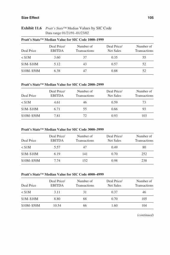
Size Effect 105
Exhibit 11.6 Pratt’s Stats™ Median Values by SIC CodeData range 01/21/91–01/23/02
Pratt’s Stats™ Median Value for SIC Code 1000–1999
Deal Price/ Number of Deal Price/ Number ofDeal Price EBITDA Transactions Net Sales Transactions
< $1M 3.60 37 0.35 55
$1M–$10M 5.12 43 0.57 52
$10M–$50M 6.38 47 0.88 52
Pratt’s Stats™ Median Value for SIC Code 2000–2999
Deal Price/ Number of Deal Price/ Number ofDeal Price EBITDA Transactions Net Sales Transactions
< $1M 4.61 46 0.59 73
$1M–$10M 6.71 55 0.66 93
$10M–$50M 7.81 72 0.93 103
Pratt’s Stats™ Median Value for SIC Code 3000–3999
Deal Price/ Number of Deal Price/ Number ofDeal Price EBITDA Transactions Net Sales Transactions
< $1M 5.57 47 0.49 80
$1M–$10M 6.19 141 0.70 252
$10M–$50M 7.74 152 0.98 238
Pratt’s Stats™ Median Value for SIC Code 4000–4999
Deal Price/ Number of Deal Price/ Number ofDeal Price EBITDA Transactions Net Sales Transactions
< $1M 3.11 31 0.37 46
$1M–$10M 8.80 68 0.70 105
$10M–$50M 10.54 66 1.60 104
(continued)
3953 P-11 8/29/02 2:23 PM Page 105
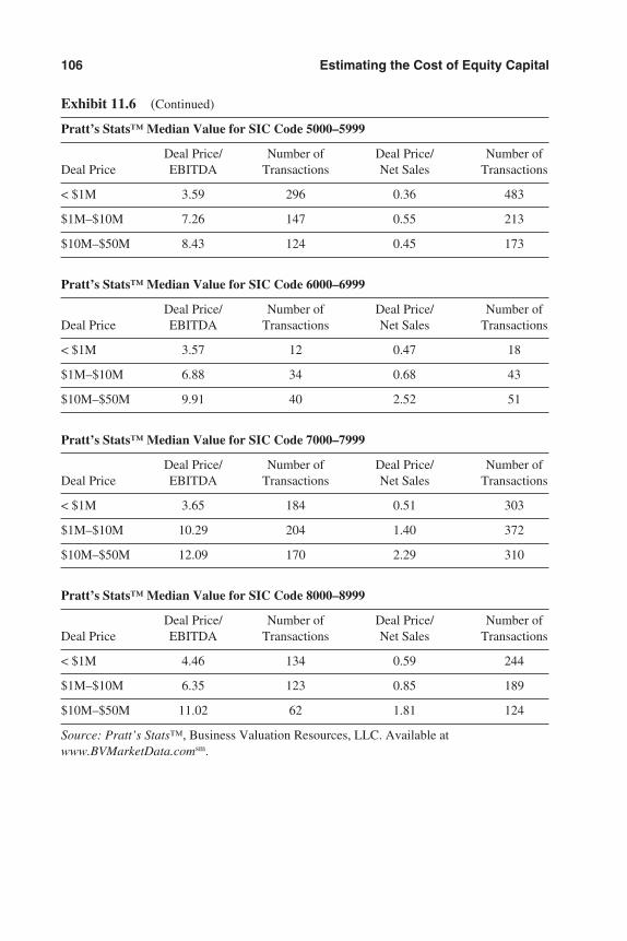
106 Estimating the Cost of Equity Capital
Exhibit 11.6 (Continued)
Pratt’s Stats™ Median Value for SIC Code 5000–5999
Deal Price/ Number of Deal Price/ Number ofDeal Price EBITDA Transactions Net Sales Transactions
< $1M 3.59 296 0.36 483
$1M–$10M 7.26 147 0.55 213
$10M–$50M 8.43 124 0.45 173
Pratt’s Stats™ Median Value for SIC Code 6000–6999
Deal Price/ Number of Deal Price/ Number ofDeal Price EBITDA Transactions Net Sales Transactions
< $1M 3.57 12 0.47 18
$1M–$10M 6.88 34 0.68 43
$10M–$50M 9.91 40 2.52 51
Pratt’s Stats™ Median Value for SIC Code 7000–7999
Deal Price/ Number of Deal Price/ Number ofDeal Price EBITDA Transactions Net Sales Transactions
< $1M 3.65 184 0.51 303
$1M–$10M 10.29 204 1.40 372
$10M–$50M 12.09 170 2.29 310
Pratt’s Stats™ Median Value for SIC Code 8000–8999
Deal Price/ Number of Deal Price/ Number ofDeal Price EBITDA Transactions Net Sales Transactions
< $1M 4.46 134 0.59 244
$1M–$10M 6.35 123 0.85 189
$10M–$50M 11.02 62 1.81 124
Source: Pratt’s Stats™, Business Valuation Resources, LLC. Available atwww.BVMarketData.comsm.
3953 P-11 8/29/02 2:23 PM Page 106
have an average market value of $30 million. There are literally hundreds of thou-sands of companies smaller than this for which cost of capital estimation is relevant,both for valuation and for potential project assessment purposes.
Where the data leave off seems to raise the question: Is it valid to extrapolatethese results beyond the observed population to infer even higher costs of capital forsmaller companies? From purely a statistician’s viewpoint, the answer would be no.We cannot know with certainty whether the population beyond the observed rangewould continue the trend. But most corporate finance practitioners and academicianswith whom the author has discussed this question, as well as most business brokersand merger and acquisition intermediaries, conclude that the answer is yes.
In the first edition of this book, I said “One of our goals over the next year or twois to study this issue further, which will be facilitated by the new database being de-veloped, Pratt’s Stats, covering business sale transactions all the way from $100,000 to$100 million in value.” Pratt’s Stats™ is now the official database of the InternationalBusiness Brokers Association, distributed by Business Valuation Resources, LLC, on-line at www.BVMarketData.comsm. It covers business sales with a market value of in-vested capital from under $100,000 to $1 billion.
Most of the companies in Ibbotson’s 10b and S&P CVC’s 25th size category havemarket capitalizations between $10 million and $50 million. In order to test the hy-pothesis that it would be valid to extrapolate the trend to companies smaller than $10million, we calculated median transaction value multiples (market value of investedcapital [MVIC]/EBITDA and MVIC/sales) for eight broad industry groups for trans-actions with $10 million to $50 million MVIC, $1 million to $10 million, and under$1 million. The results are shown in Exhibit 11.6.
As shown, for every broad industry group, median price EBITDA multiples werelower for the $1 million to $10 million group than for the $10 million to $50 milliongroup, and lower yet for the under $1 million group. Similar results, although lessconsistent for a few industries, were observed for the deal price/sales multiples. I be-lieve that this provides further strong evidence that the size effect does indeed existand that it is valid to extrapolate it for companies with market values of equity below$10 million.
SUMMARY
Three independent sets of empirical studies provide strong support for the propo-sition that cost of capital tends to increase with decreasing company size. Users ofcost of capital data should make themselves aware of updates of these and possiblyother similar studies to incorporate the latest current size effect data in cost of capitalestimates, whether using build-up models, CAPM, or other cost of equity models.The data currently available provide empirical evidence to help quantify the cost ofcapital for smaller companies, and the subject is attracting considerable new researchinterest.
Size Effect 107
3953 P-11 8/29/02 2:23 PM Page 107

Notes
1. Stocks, Bonds, Bills & Inflation, Valuation Edition 2001 Yearbook (Chicago: IbbotsonAssociates, 2001), 123.
2. Tyler Shumway, “The Delisting Bias in CRSP Data,” Journal of Finance (March 1997).3. See “New Studies Quantifying Size Premiums Offer Strong Cost of Capital Support,”
Shannon Pratt’s Business Valuation Update® (August 1997): 1–3; see also ShannonPratt, “New Measures of Risk That Really Work,” Shannon Pratt’s Business ValuationUpdate® (December 1999): 1–4; and see Roger Grabowski and David King, “The SizeEffect and Equity Returns,” Appendix 5A in Jay Fishman et al., Guide to Business Valu-ations, 12th ed. (Forth Worth, TX: Practitioners Publishing Company, 2001), 5–75 et seq.
4. PricewaterhouseCoopers Risk Premium Study 2000, p. 12 (now the Standard & Poor’sCorporate Value Consulting Risk Premium Reports).
108 Estimating the Cost of Equity Capital
3953 P-11 8/29/02 2:23 PM Page 108
109
Chapter 12
DCF Method of EstimatingCost of CapitalTheory of the DCF MethodMechanics of the DCF MethodSingle-stage DCF ModelMultistage DCF ModelsSources of InformationSummary
As discussed earlier in this book, there are several ways to estimate the cost ofequity capital. Up to this point, all of the methods have had one thing in common:They begin with a risk-free rate and add one or many factors, based on the risks of theinvestment. The discounted cash flow (DCF) method is completely different.
THEORY OF THE DCF METHOD
At least in theory, the DCF method is more direct and simpler than the build-upmodel or the Capital Asset Pricing Model. The important assumption of the DCFmethod is that the public company’s current stock price embodies the market’s ex-pectation of the rate of return that will be realized by investing in that stock.
In other words, the assumption is that the current stock price is actually the sumof the present values of the expected future returns to the investors (dividends andstock price change). The implied assumption is that the current stock price is equal tothe expected future returns discounted to a present value at a discount rate that rep-resents the equity cost of capital for that company.
The theory of the DCF method to estimate cost of capital is to use the DCF for-mula for computing present value backward. That is, since the present value (i.e., thecurrent stock price) is known, the calculations are reconfigured to solve for ke, thecost of equity capital.
The relationship between the DCF method of valuing a business and the DCFmethod of estimating cost of capital is the matter of which are the known and un-known variables. In using the DCF method to value a company, division, or project,the cost of capital already has been estimated and is given as a known rate in the for-mula to estimate the present value. In using the DCF method to estimate the cost of
3953 P-12 8/29/02 2:23 PM Page 109
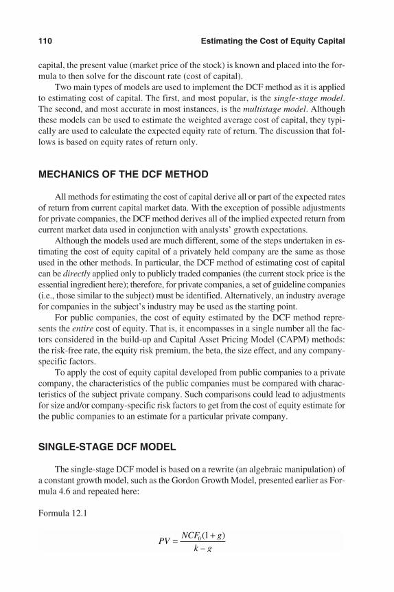
capital, the present value (market price of the stock) is known and placed into the for-mula to then solve for the discount rate (cost of capital).
Two main types of models are used to implement the DCF method as it is appliedto estimating cost of capital. The first, and most popular, is the single-stage model.The second, and most accurate in most instances, is the multistage model. Althoughthese models can be used to estimate the weighted average cost of capital, they typi-cally are used to calculate the expected equity rate of return. The discussion that fol-lows is based on equity rates of return only.
MECHANICS OF THE DCF METHOD
All methods for estimating the cost of capital derive all or part of the expected ratesof return from current capital market data. With the exception of possible adjustmentsfor private companies, the DCF method derives all of the implied expected return fromcurrent market data used in conjunction with analysts’ growth expectations.
Although the models used are much different, some of the steps undertaken in es-timating the cost of equity capital of a privately held company are the same as thoseused in the other methods. In particular, the DCF method of estimating cost of capitalcan be directly applied only to publicly traded companies (the current stock price is theessential ingredient here); therefore, for private companies, a set of guideline companies(i.e., those similar to the subject) must be identified. Alternatively, an industry averagefor companies in the subject’s industry may be used as the starting point.
For public companies, the cost of equity estimated by the DCF method repre-sents the entire cost of equity. That is, it encompasses in a single number all the fac-tors considered in the build-up and Capital Asset Pricing Model (CAPM) methods:the risk-free rate, the equity risk premium, the beta, the size effect, and any company-specific factors.
To apply the cost of equity capital developed from public companies to a privatecompany, the characteristics of the public companies must be compared with charac-teristics of the subject private company. Such comparisons could lead to adjustmentsfor size and/or company-specific risk factors to get from the cost of equity estimate forthe public companies to an estimate for a particular private company.
SINGLE-STAGE DCF MODEL
The single-stage DCF model is based on a rewrite (an algebraic manipulation) ofa constant growth model, such as the Gordon Growth Model, presented earlier as For-mula 4.6 and repeated here:
Formula 12.1
PVNCF g
k g= +0 1( )
–
110 Estimating the Cost of Equity Capital
3953 P-12 8/29/02 2:23 PM Page 110
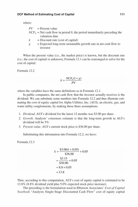
where:
PV = Present valueNCF0 = Net cash flow in period 0, the period immediately preceding the
valuation datek = Discount rate (cost of capital)g = Expected long-term sustainable growth rate in net cash flow to
investor
When the present value (i.e., the market price) is known, but the discount rate(i.e., the cost of capital) is unknown, Formula 12.1 can be rearranged to solve for thecost of capital:
Formula 12.2
where the variables have the same definitions as in Formula 12.1.In public companies, the net cash flow that the investor actually receives is the
dividend. We can substitute some numbers into Formula 12.2 and thus illustrate esti-mating the cost of equity capital for Alpha Utilities, Inc. (AUI), an electric, gas, andwater utility conglomerate, by making these three assumptions:
1. Dividend. AUI’s dividend for the latest 12 months was $3.00 per share.
2. Growth. Analysts’ consensus estimate is that the long-term growth in AUI’sdividend will be 5%.
3. Present value. AUI’s current stock price is $36.00 per share.
Substituting this information into Formula 12.2, we have:
Formula 12.3
Thus, according to this computation, AUI’s cost of equity capital is estimated to be13.8% (8.8% dividend yield plus 5.0% expected stock price increase).
The preceding is the formulation used in Ibbotson Associates’ Cost of CapitalYearbook “Analysts Single-Stage Discounted Cash Flow” cost of equity capital
k = + +
= +
= +=
$ . ( . )
$ ..
$ .
$ ..
. .
.
3 00 1 0 05
36 000 05
3 15
36 000 05
8 8 0 05
13 8
kNCF g
PV= +0 1( )
DCF Method of Estimating Cost of Capital 111
3953 P-12 8/29/02 2:23 PM Page 111
estimate. Ibbotson’s source of growth estimates is the I/B/E/S database (now Thom-son Financial) of consensus long-term growth rate estimates. A number of othersources of growth estimates are included in Appendix C.
This single-stage DCF model often is used in utility rate hearings to estimate autility’s cost of equity.1
Like the capitalization “shortcut” version of the discounting model used for valu-ation, the single-stage DCF model for estimating cost of capital is deceptively simple.
In utility settings, the dividend yield is assumed to be an appropriate estimate ofthe first input, cash flow yield. This is reasonable, because publicly traded utilitiestypically pay dividends, and these dividends represent a high percentage of availablecash flows. In cases where the utility’s dividend yield is abnormally high or low, a“normal” dividend yield is used. It is difficult, however, to use dividend yields withall publicly traded companies.
For many companies, dividend payments may have little to do with earnings orcash flows. A large number of companies do not pay dividends or pay only a tokenamount. In these cases, theoretically, the growth component, g, will be larger thanthat of an otherwise similar company that pays higher dividends. In practice, properlyadjusting for this lack of dividends is extremely difficult.
One way to avoid the dividend issue is to define cash flows more broadly. In-stead of considering only the cash flows investors actually receive (dividends), theanalyst might define net cash flows as those amounts that could be paid to equity in-vestors without impeding a company’s future growth. As noted in Chapter 3, net cashflow is usually defined as:
Net income (after tax)
+ Noncash charges (e.g., depreciation, amortization, deferred revenue,deferred taxes)
– Capital expenditures*– Additions to net working capital*± Changes in long-term debt (add cash from borrowing, subtract repayments)*———————————————————————————————= Net cash flow to equity
*Only amounts necessary to support projected operations
Of course, these cash flows are not those paid to investors, but, presumably, in-vestors ultimately will realize the benefit of these amounts through higher future div-idends, a special dividend, or, more likely, stock price appreciation. Some analystsassume that over the very long run, net (after-tax) income should be quite close to cashflows. Therefore, they assume that net income can be used as a proxy for net cashflow. This assumption should be questioned on a case-by-case basis. For a growingcompany, capital expenditure and working capital requirements may make the as-sumed equivalence of net income and net cash flow so remote as to be irrelevant.
The other, and perhaps more problematic, input is the expected growth rate. Animportant characteristic of the growth rate is that it is the perpetual annual growth rate.
112 Estimating the Cost of Equity Capital
3953 P-12 8/29/02 2:23 PM Page 112
Future growth rates do not have to be the same for every year; however, the “average”rate should be equal to this perpetual rate. For example, if a company is expected togrow at 10% per year for the next four years and 3% per year thereafter, then the av-erage growth rate into perpetuity could be estimated as about 5%. On the other hand,if the company is expected to grow by 10% per year for the next 20 years and 3% peryear thereafter, the average growth rate is probably closer to 9%. However, this wouldbe an extreme case. It is theoretically impossible for the sustainable perpetual growthrate for a company to significantly exceed the growth rate in the economy. Anythingover a 6–7% perpetual growth rate should be questioned carefully.
A common approach to deriving a perpetual growth rate is to obtain stock ana-lysts’ estimates of earnings growth rates. The advantage of using these growth esti-mates is that they are prepared by people who follow these companies on an ongoingbasis. These professional stock analysts develop a great deal more insight on thesecompanies than a casual investor or valuation analyst not specializing in the industryis likely to achieve.
There are, however, three caveats when using this information:
1. These earnings growth estimates typically are for only the next two to five years;they are not perpetual. Therefore, any use of these forecasts in a single-stageDCF model must be tempered with a longer-term forecast.
2. Most published analysts’ estimates come from “sell-side” stock analysts whowork for firms that are in business to sell stocks. Thus, although their earningsforecasts fall within the range of “reasonable” possibilities, they may be on thehigh end of the range.
3. Usually these estimates are obtained from firms that provide consensus earningsforecasts; that is, they aggregate forecasts from a number of analysts and reportcertain summary statistics (mean, median, etc.) on these forecasts. For a smallpublicly traded firm, there may be only one or even no analyst following thecompany. The potential for forecasting errors is greater when the forecasts areobtained from a very small number of analysts. These services typically reportthe number of analysts who have provided earnings estimates, which should beconsidered in determining how much reliance to place on forecasts of this type.
Many of the problems inherent in using the single-stage model to estimate costof capital are addressed by using a multistage model.
MULTISTAGE DCF MODELS
Multistage models come closer to reversing the discounting process than dosingle-stage models that simply reverse the capitalization process. Multistage mod-els do not go to the extent of incorporating specific expected return amounts for spe-cific years, but they do incorporate different growth rates for different expected growthstages, most often three stages.
DCF Method of Estimating Cost of Capital 113
3953 P-12 8/29/02 2:23 PM Page 113
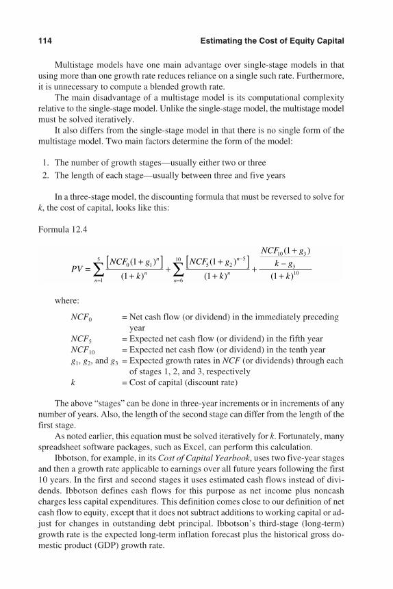
Multistage models have one main advantage over single-stage models in thatusing more than one growth rate reduces reliance on a single such rate. Furthermore,it is unnecessary to compute a blended growth rate.
The main disadvantage of a multistage model is its computational complexityrelative to the single-stage model. Unlike the single-stage model, the multistage modelmust be solved iteratively.
It also differs from the single-stage model in that there is no single form of themultistage model. Two main factors determine the form of the model:
1. The number of growth stages—usually either two or three
2. The length of each stage—usually between three and five years
In a three-stage model, the discounting formula that must be reversed to solve fork, the cost of capital, looks like this:
Formula 12.4
where:
NCF0 = Net cash flow (or dividend) in the immediately precedingyear
NCF5 = Expected net cash flow (or dividend) in the fifth yearNCF10 = Expected net cash flow (or dividend) in the tenth yearg1, g2, and g3 = Expected growth rates in NCF (or dividends) through each
of stages 1, 2, and 3, respectivelyk = Cost of capital (discount rate)
The above “stages” can be done in three-year increments or in increments of anynumber of years. Also, the length of the second stage can differ from the length of thefirst stage.
As noted earlier, this equation must be solved iteratively for k. Fortunately, manyspreadsheet software packages, such as Excel, can perform this calculation.
Ibbotson, for example, in its Cost of Capital Yearbook, uses two five-year stagesand then a growth rate applicable to earnings over all future years following the first10 years. In the first and second stages it uses estimated cash flows instead of divi-dends. Ibbotson defines cash flows for this purpose as net income plus noncashcharges less capital expenditures. This definition comes close to our definition of netcash flow to equity, except that it does not subtract additions to working capital or ad-just for changes in outstanding debt principal. Ibbotson’s third-stage (long-term)growth rate is the expected long-term inflation forecast plus the historical gross do-mestic product (GDP) growth rate.
PVNCF g
k
NCF g
k
NCF g
k g
k
n
n
n
nnn
=+[ ]
++
+[ ]+
+
+
+==∑∑ 0 1 5 2
510 3
310
6
10
1
5 1
1
1
1
1
1
( )
( )
( )
( )
( )
–
( )
–
114 Estimating the Cost of Equity Capital
3953 P-12 8/29/02 2:23 PM Page 114
SOURCES OF INFORMATION
To perform the DCF cost of capital analysis rather than use data compiled by oneof the services, a variety of inputs is necessary, including company-specific data, in-dustry outlook data, and long-term macroeconomic forecasts.
Company data can be obtained from Securities and Exchange Commission (SEC)filings or services such as Standard & Poor’s (a division of McGraw-Hill), Moody’s(published by Mergent, Inc.), and Value Line Publishing, Inc. Analysts’ estimates canbe compiled from individual analysts’ reports or from one of the three earnings con-sensus reporting services: Thomson Financial (formerly First Call and I/B/E/S), Mul-tex-Ace, and Zack’s Investment Research, Inc.
There are a great number of different industry forecasts. For some industries, ex-cellent material is available from industry trade associations, although they tend tofocus primarily on revenues rather than on cash flows. There is also a wide variety ofmacroeconomic forecast information. Appendix C lists details on many sources pro-viding data in all these categories. A more comprehensive compilation of the industryforecasts is the Business Valuation Data, Publications & Internet Directory, pub-lished annually by Business Valuation Resources, LLC, (888) BUS-VALU [(888)287-8258], www.BVResources.com.
SUMMARY
The DCF method of cost of capital estimation attempts to use current public stockprice information to estimate implied costs of equity capital. Single-stage models usea Gordon Growth Model type of formula, with the present value (i.e., the stock price)known, solving for k, the cost of capital. Multistage models use two or more growthestimates for different future periods. As with the CAPM, applying the method to pri-vately held companies involves using public companies in a similar industry group todevelop a proxy starting point, with modifications for differences in the characteristicsbetween the public guideline companies and the subject company.
Analysts can obtain DCF-based cost of capital estimates for public companiesand industries from several services that compile them or can build their own esti-mates from scratch.
The author is working on a research paper showing examples of applying theDCF method of estimating the cost of capital using several different sources of growthestimates. Readers may obtain a complimentary copy of this research paper when it iscompleted by contacting the author at the address shown in the preface.
Note
1. For a concise discussion of the use of this model for utility rate-setting, see Richard A.Brealey and Stewart C. Myers, Principles of Corporate Finance, 6th ed. (Boston: IrwinMcGraw-Hill, 2000), 67–69.
DCF Method of Estimating Cost of Capital 115
3953 P-12 8/29/02 2:23 PM Page 115
116
Chapter 13
Using Ibbotson AssociatesCost of Capital DataMichael W. Barad and Tara McDowell
Stocks, Bonds, Bills and InflationCost of Equity ModelsEquity Risk PremiumFirm Size PremiumIndustry PremiumIbbotson Data and TaxesIbbotson Data: Minority or Controlling Interest?
Cost of Capital YearbookOrganization of DataCost of Equity ModelsCapital Asset Pricing Model Fama-French Three-factor ModelDiscounted Cash Flow Models
Ibbotson Beta BookBeta Estimation MethodologiesLevered and Unlevered BetasIbbotson (Adjusted) BetasPeer Group and Industry Betas
Cost of Capital Center
Notation for This Chapter: The notation used in this chapter is that used in theIbbotson data sources discussed herein and may differ slightly from the notation usedelsewhere in this book. There are, however, no conceptual discrepancies betweenequations in this chapter and similar equations elsewhere in this book.
Ibbotson Associates is a financial software, data, consulting, and training firmheadquartered in Chicago, Illinois. Established in 1977 by Roger Ibbotson, IbbotsonAssociates is a leading provider of financial information to business valuation ana-lysts, corporate finance professionals, and investment analysts. Ibbotson produces fourpublications that valuation and corporate finance professionals at all levels have founduseful in the estimation of the cost of capital for companies of various industries andsizes.
The firm’s benchmark publication is the Stocks, Bonds, Bills and Inflation (SBBI)Yearbook. Now commonly referred to as the Classic Edition, the SBBI Yearbook is
3953 P-13 8/29/02 2:24 PM Page 116
based on Roger Ibbotson and Rex Sinquefield’s original 1976 study of long-term mar-ket analysis. This publication has become a staple in the field of finance and is updatedannually by Ibbotson Associates. The SBBI Yearbook is a leading source for histori-cal market data, including data on the equity risk premium and firm size premium,market commentary, and other historical analysis on the capital markets.
While the SBBI Classic Edition Yearbook served as the foundation for discountrate, capitalization rate, and cost of capital estimates for many years, the introduction ofthe Stocks, Bonds, Bills, and Inflation Valuation Edition Yearbook has become the newstandard for such valuation data. The SBBI Valuation Edition Yearbook was first intro-duced in 1999 to address the growing data needs of the valuation profession. The Val-uation Edition was authored by Michael Annin and Dominic Falaschetti and expandedgreatly on the cost of capital data already presented in the Classic Edition by drawingprimarily from the cost of capital workshops then held by Ibbotson Associates. TheValuation Edition, updated annually by Ibbotson Associates, not only presents dataalong with examples on how to use it, but also addresses topical issues and controver-sies each year with alternative calculation methods and new studies as they becomeavailable. The Valuation Edition focuses primarily on the equity risk premium, size pre-mium, industry premium, beta, and other issues related to the cost of capital.
Ibbotson Associates’ Cost of Capital Yearbook is another publication geared di-rectly to business valuation and corporate finance decisions. Ibbotson has published theCost of Capital Yearbook, formerly referred to as Cost of Capital Quarterly (CCQ),since 1994. The Cost of Capital Yearbook is an industry analysis publication that pre-sents cost of capital and other financial information useful in business valuation andcorporate finance. Over 300 industries organized by Standard Industrial Classification(SIC) code are presented in the Cost of Capital Yearbook. While the yearbook is pub-lished annually with data through March, quarterly updates are available.
The Beta Book rounds out Ibbotson’s library of publications. Published semian-nually since 1995, the Beta Book provides beta and three-factor model information onmore than 5,000 companies. The Beta Book allows practitioners to select a company-specific measure of risk directly applicable to a publicly traded company, or to con-struct a custom peer group for analysis of a private company. This chapter discussesIbbotson Associates publications in detail.
STOCKS, BONDS, BILLS AND INFLATION
Ibbotson’s Stocks, Bonds, Bills and Inflation (SBBI) Classic Edition Yearbook andValuation Edition Yearbook are some of the most commonly cited references in val-uation reports. The Classic Edition, as it is now known, is based on the original studyof long-term capital market performance done by Roger Ibbotson and Rex Sinque-field in 1976. The Classic Edition was first published in 1983 to satisfy the demandfor a comprehensive historical data set along with corresponding analysis on the cap-ital markets. The Valuation Edition was first published in 1999 to expand on the cost
Using Ibbotson Associates Cost of Capital Data 117
3953 P-13 8/29/02 2:24 PM Page 117
of capital concepts and data covered in both the Classic Edition and Ibbotson’s costof capital workshops. Both publications are updated annually by Ibbotson Associates.
While both yearbooks provide discussions and estimates of the equity risk pre-mium and firm size premium, the Valuation Edition focuses primarily on the scienceof valuation and has much greater coverage on topics related to the cost of capital.The Valuation Edition discusses current issues and controversies related to cost ofcapital and includes any of Ibbotson’s advances in the field of cost of capital analy-sis. Some examples of such coverage presented only in the Valuation Edition wouldbe the inclusion of industry premia for use in the build-up method and alternativemeasures of firm size premia, including a further breakout of the smallest companies(the tenth decile) into even smaller divisions (10a and 10b). While the Classic Editionstill provides much useful information to the valuation industry in the form of capi-tal market analysis and discussions on the performance of the economy, the Valua-tion Edition is critical to anyone performing cost of capital analysis using the incomeapproach and has become the industry standard for such data. For this reason, it is theValuation Edition that serves as the basis for the following discussion.
Cost of Equity Models
The cost of equity capital is equal to the expected rate of return for a firm’s equity.There are several widely used models for estimating cost of equity for a firm, the twomost common being the build-up method and the Capital Asset Pricing Model (CAPM)(see Exhibit 13.1). Other methods such as the Fama-French three-factor model and thediscounted cash flow model will be discussed later. Both the build-up method and theCAPM are very similar, with the major exception being the use of beta.
The risk-free rate, equity risk premium, and firm size premium are componentsshared by both the build-up method and the CAPM. These models should provide verysimilar if not identical results if implemented correctly. Let us take a private companyas an example. For a private company, there is no market data to derive a beta. There-fore, to use the CAPM the analyst must use a beta from comparable companies. If weassume that the beta used in this example is an industry beta for the subject company’sindustry, then both the build-up and CAPM models have a provision for including in-dustry risk. Theoretically, the industry premium in the build-up model and the indus-try beta used in the CAPM should lead both models toward identical results.
Equity Risk Premium
The expected equity risk premium is defined as the additional return investorsexpect to receive to compensate for the additional risk associated with investing inequities as opposed to riskless assets. The equity risk premium is a critical componentof many of the cost of equity models, including the build-up method, CAPM, andFama-French three-factor model.
While the equity risk premium (ERP) has many uses throughout the field of fi-nance, for the purpose of business valuation it should be a forward-looking measure
118 Estimating the Cost of Equity Capital
3953 P-13 8/29/02 2:24 PM Page 118
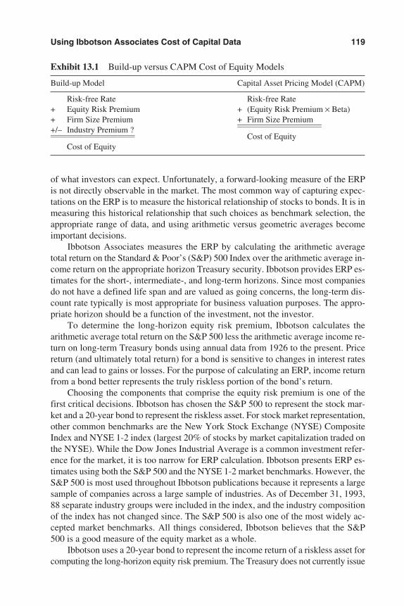
of what investors can expect. Unfortunately, a forward-looking measure of the ERPis not directly observable in the market. The most common way of capturing expec-tations on the ERP is to measure the historical relationship of stocks to bonds. It is inmeasuring this historical relationship that such choices as benchmark selection, theappropriate range of data, and using arithmetic versus geometric averages becomeimportant decisions.
Ibbotson Associates measures the ERP by calculating the arithmetic averagetotal return on the Standard & Poor’s (S&P) 500 Index over the arithmetic average in-come return on the appropriate horizon Treasury security. Ibbotson provides ERP es-timates for the short-, intermediate-, and long-term horizons. Since most companiesdo not have a defined life span and are valued as going concerns, the long-term dis-count rate typically is most appropriate for business valuation purposes. The appro-priate horizon should be a function of the investment, not the investor.
To determine the long-horizon equity risk premium, Ibbotson calculates thearithmetic average total return on the S&P 500 less the arithmetic average income re-turn on long-term Treasury bonds using annual data from 1926 to the present. Pricereturn (and ultimately total return) for a bond is sensitive to changes in interest ratesand can lead to gains or losses. For the purpose of calculating an ERP, income returnfrom a bond better represents the truly riskless portion of the bond’s return.
Choosing the components that comprise the equity risk premium is one of thefirst critical decisions. Ibbotson has chosen the S&P 500 to represent the stock mar-ket and a 20-year bond to represent the riskless asset. For stock market representation,other common benchmarks are the New York Stock Exchange (NYSE) CompositeIndex and NYSE 1-2 index (largest 20% of stocks by market capitalization traded onthe NYSE). While the Dow Jones Industrial Average is a common investment refer-ence for the market, it is too narrow for ERP calculation. Ibbotson presents ERP es-timates using both the S&P 500 and the NYSE 1-2 market benchmarks. However, theS&P 500 is most used throughout Ibbotson publications because it represents a largesample of companies across a large sample of industries. As of December 31, 1993,88 separate industry groups were included in the index, and the industry compositionof the index has not changed since. The S&P 500 is also one of the most widely ac-cepted market benchmarks. All things considered, Ibbotson believes that the S&P500 is a good measure of the equity market as a whole.
Ibbotson uses a 20-year bond to represent the income return of a riskless asset forcomputing the long-horizon equity risk premium. The Treasury does not currently issue
Using Ibbotson Associates Cost of Capital Data 119
Exhibit 13.1 Build-up versus CAPM Cost of Equity Models
Build-up Model Capital Asset Pricing Model (CAPM)
Risk-free Rate Risk-free Rate+ Equity Risk Premium + (Equity Risk Premium × Beta)+ Firm Size Premium + Firm Size Premium+/– Industry Premium ?
————————————————————
————————————————————
Cost of EquityCost of Equity
3953 P-13 8/29/02 2:24 PM Page 119
20-year bonds, however. Both 10-year and 30-year bonds are possible benchmark op-tions, but Ibbotson chooses to use bonds on the market with approximately 20 years tomaturity to keep the basis of the time series consistent across time. The Treasury didnot issue 30-year or 10-year bonds as far back as 1926, and as of the date of this pub-lication the Treasury had stopped issuing 30-year bonds altogether. Ibbotson believesthat the best option for a consistent time series of long-term bond data extending backto 1926 is the 20-year bond.
The SBBI equity risk premium covers the time range from 1926 to present. Theoriginal data source for the raw data series comprising the ERP is the Center for Re-search in Security Prices (CRSP) at the University of Chicago. The CRSP chose 1926as a starting date for its data series because this is when good-quality financial databecame available. This period was chosen also because it includes one full businesscycle before the 1929 market crash. While Roger Ibbotson and other researchershave published data back to the early nineteenth century, these data are not of the samequality as the data that begin in 1926. In basic terms, these are the main reasons whyIbbotson uses a range back to 1926 in equity risk premium calculations.
The period from 1926 to present is most relevant because it includes a numberof different economic scenarios. Some practitioners argue for a shorter historical pe-riod, such as the last 20 or 30 years. This argument is based on the assumption that in-vestors only factor in a more recent economic climate into their expectations and that“unusual” economic events prior to recent times are not likely to repeat in the future.All periods contain unusual events, some of which took place most recently. For ex-ample, the inflation of the late 1970s and early 1980s, the October 1987 market crash,the collapse of the Soviet Union, the development of the European Economic Com-munity, and the September 2001 terrorist attack on the United States are but a few ofthe “unusual” events that occurred in recent times. While we do not expect these eventsto occur again in the future, they are representative of the type of events that canoccur unexpectedly and have massive effects on the economy. Focusing on a shorterhistorical date range would magnify the effect of the most recent unusual events. Usinga longer range of data places less emphasis on each event and better captures long-term performance. By including market data measured over the entire set of economicscenarios available, Ibbotson believes that the resulting computations can better an-ticipate similar events in the future.
The equity risk premium presented by Ibbotson Associates is an arithmetic av-erage risk premium, as opposed to a geometric average risk premium. Ibbotson believesthat arithmetic averages are appropriate for use in discounting future cash flows. Ageometric average is better for reporting past performance since it represents the com-pound average return. Mathematically, the arithmetic mean assumes that the cash flowbeing discounted each period is the expected value of the probability distribution ofpossible outcomes for that period.
Arithmetic averages better incorporate the volatility in a data series. Take bondsand stocks as an example. Bonds have lower volatility than stocks, on average. Whencomparing the arithmetic mean with the geometric mean for each asset class, the dif-ference between arithmetic and geometric will be greater for the asset class with highervolatility. The arithmetic mean captures the volatility of a time series. Since the ERP
120 Estimating the Cost of Equity Capital
3953 P-13 8/29/02 2:24 PM Page 120
is a volatile data set and we are using it in a forward-looking capacity, the arithmetic av-erage will better capture the uncertainty associated with the ERP. In general terms,arithmetic averages are better forward-looking point estimates, and geometric averagesare better for historical analysis of a defined data range.
Numerous alternatives to using pure historical data for calculating the equity riskpremium bear discussion. A few of these methods for calculating ERP are:
• The use of survey results
• The exponential weighting of historical periods
• The supply-side perspective
The first of these alternatives takes the approach that a survey of ERP expectationsfrom the appropriate people will yield more useful information. Typically, the surveyis conducted on academics, money managers, or other professionals deemed to have aneducated idea on the direction of the market. The difficulty in relying on this methodstems from the subjective nature of the “opinions” submitted by the participants, alongwith a bias for participants to form estimates based heavily on the current economiccondition.
For those who struggle with the appropriate time period to use in their historicalERP calculation, exponential weighting offers a solution. Using an exponential weight-ing scheme to average historical data allows for more importance to be placed on cur-rent data (compared with an equal weighting scheme). Of course, this assumes thatan unbiased reason exists for assuming that the future will bring with it an economicclimate more similar to that of recent periods.
The last alternative to calculating the ERP is the supply-side model. This methodestimates what the economy can supply going forward, as opposed to its actual his-torical performance. In general, research has shown that the supply-side estimate islower than the historical estimate, indicating that the market cannot supply the typeof long-term growth that it has demonstrated to date.
All of the alternatives to estimating ERP have advantages and disadvantages. Forcost of capital analysis, it is important that all of the cost-of-equity components aredeveloped so they can work together in a model. If using a size premium, industrypremium, or any other addition to the cost of equity, it is imperative that all of thecomponents be on the same basis. For example, the time period and weighting schemeof the ERP and size premium should be identical. Similarly, both components shouldbe from either a historical perspective or a supply-side perspective. Consistency is acritical attribute in cost of capital analysis.
Firm Size Premium
The relationship between firm size and return is one of the most remarkable dis-coveries of modern finance. This relationship cuts across the entire size spectrum butis most evident among smaller companies. While many studies have examined the sizeeffect, Ibbotson Associates is the most cited source of size premium data as publishedin both the SBBI Classic Edition Yearbook and the SBBI Valuation Edition Yearbook.
Using Ibbotson Associates Cost of Capital Data 121
3953 P-13 8/29/02 2:24 PM Page 121
What is the firm size premium? Historically, small stocks have shown greaterrisk and greater return than their larger capitalization counterparts. This makes perfectsense since investors will demand higher return to compensate for increased risk. Ifsmall stocks did not provide a higher return to compensate for this risk, there wouldbe no demand to invest in them. To capture the additional return exhibited by smallerstocks, we calculate a size premium that can be used as an addition to either the CAPMor build-up model of estimating cost of equity.
The first point worth noting is the evolution of Ibbotson’s size premium and thedifference between what is presented in the Classic Edition and Valuation Editionyearbooks. Through the 1994 yearbook, the Classic Edition simply presented what Ib-botson calls the small stock premium. The small stock premium was measured as thesimple difference between Ibbotson’s Small Company Stock series and the S&P 500total returns. The Small Company Stock series is a representation of publicly tradedmicro-cap stocks. Beginning in 1995, the SBBI Classic Edition presented a chapter onfirm size that analyzed the small stock effect across all 10 deciles of the stock mar-ket. At this point the CRSP data for companies traded on the NYSE was used in thefirm size analysis. At the same time that data was introduced for all 10 deciles, a newmethod for measuring the size effect was introduced. This new method was calculatedas the return in excess of what CAPM predicts given the beta for a decile, otherwiseknown as a beta-adjusted size premium. In 1999 Ibbotson Associates introduced thefirst SBBI Valuation Edition Yearbook. The Valuation Edition was created to addresscurrent topics relating primarily to cost of capital analysis and to present advancesmade in this field. While a firm size chapter exists in both yearbooks, the Valuation Edi-tion has much more extensive coverage and analysis on the topic of firm size. The re-mainder of this section discusses some of the coverage offered in the Valuation Edition.
The Valuation Edition Yearbook has continued to present advances in firm sizeanalysis since its inception in 1999. Beginning with the 2001 edition, the yearbook re-vised all size premium calculations to include the population of stocks traded on theNew York Stock Exchange (NYSE), American Stock Exchange (AMEX), and NasdaqStock Market (Nasdaq). The AMEX and Nasdaq securities were added to the analysisto capture the performance of the many small stocks traded on these exchanges. TheNYSE is used to create the breakpoints that define the deciles, to which AMEX andNasdaq securities of similar size are then added. Also in the 2001 edition, size premiawere added for deciles 10a and 10b. This breakout of the tenth decile into two com-ponents allows for further analysis of the smallest companies. Additional statistics re-lating to 10a and 10b were presented beginning in the 2002 yearbook.
Exhibit 13.2 is a graph from the SBBI Valuation Edition 2001 Yearbook showingthe actual returns achieved by the 10 deciles and the security market line on which theCAPM would predict the portfolios would fall. If the CAPM were functioning prop-erly, all of the decile portfolios would fall directly on the line indicated on the graph.Instead, most of the deciles fall above the security market line, indicating that theCAPM underreports cost of equity for all but the largest companies. The vertical spacebetween a decile and the security market line is the graphical representation of thesize premium. This premium must be added back into the cost of equity to fully explainthe returns of all but the largest companies.
122 Estimating the Cost of Equity Capital
3953 P-13 8/29/02 2:24 PM Page 122
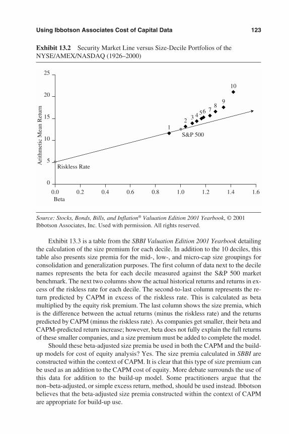
Exhibit 13.3 is a table from the SBBI Valuation Edition 2001 Yearbook detailingthe calculation of the size premium for each decile. In addition to the 10 deciles, thistable also presents size premia for the mid-, low-, and micro-cap size groupings forconsolidation and generalization purposes. The first column of data next to the decilenames represents the beta for each decile measured against the S&P 500 marketbenchmark. The next two columns show the actual historical returns and returns in ex-cess of the riskless rate for each decile. The second-to-last column represents the re-turn predicted by CAPM in excess of the riskless rate. This is calculated as betamultiplied by the equity risk premium. The last column shows the size premia, whichis the difference between the actual returns (minus the riskless rate) and the returnspredicted by CAPM (minus the riskless rate). As companies get smaller, their beta andCAPM-predicted return increase; however, beta does not fully explain the full returnsof these smaller companies, and a size premium must be added to complete the model.
Should these beta-adjusted size premia be used in both the CAPM and the build-up models for cost of equity analysis? Yes. The size premia calculated in SBBI areconstructed within the context of CAPM. It is clear that this type of size premium canbe used as an addition to the CAPM cost of equity. More debate surrounds the use ofthis data for addition to the build-up model. Some practitioners argue that thenon–beta-adjusted, or simple excess return, method, should be used instead. Ibbotsonbelieves that the beta-adjusted size premia constructed within the context of CAPMare appropriate for build-up use.
Using Ibbotson Associates Cost of Capital Data 123
Exhibit 13.2 Security Market Line versus Size-Decile Portfolios of theNYSE/AMEX/NASDAQ (1926–2000)
0.0
25
20
15
10
5
0
0.2 0.4 0.6 0.8 1.0
S&P 500
Riskless Rate
Beta
Ari
thm
etic
Mea
n R
etur
n
12 3 4 56 7
89
10
1.2 1.4 1.6
Source: Stocks, Bonds, Bills, and Inflation® Valuation Edition 2001 Yearbook, © 2001Ibbotson Associates, Inc. Used with permission. All rights reserved.
3953 P-13 8/29/02 2:24 PM Page 123
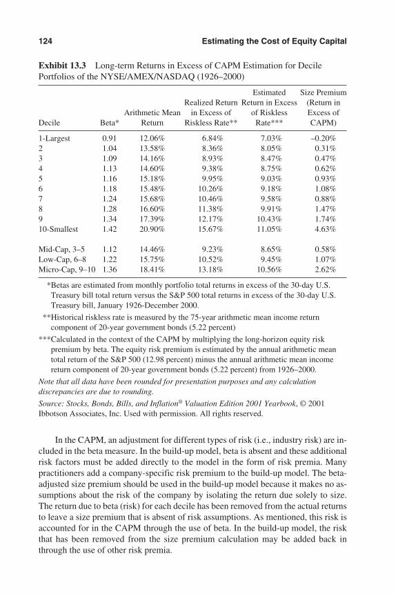
In the CAPM, an adjustment for different types of risk (i.e., industry risk) are in-cluded in the beta measure. In the build-up model, beta is absent and these additionalrisk factors must be added directly to the model in the form of risk premia. Manypractitioners add a company-specific risk premium to the build-up model. The beta-adjusted size premium should be used in the build-up model because it makes no as-sumptions about the risk of the company by isolating the return due solely to size.The return due to beta (risk) for each decile has been removed from the actual returnsto leave a size premium that is absent of risk assumptions. As mentioned, this risk isaccounted for in the CAPM through the use of beta. In the build-up model, the riskthat has been removed from the size premium calculation may be added back inthrough the use of other risk premia.
124 Estimating the Cost of Equity Capital
Exhibit 13.3 Long-term Returns in Excess of CAPM Estimation for DecilePortfolios of the NYSE/AMEX/NASDAQ (1926–2000)
Estimated Size PremiumRealized Return Return in Excess (Return in
Arithmetic Mean in Excess of of Riskless Excess ofDecile Beta* Return Riskless Rate** Rate*** CAPM)
1-Largest 0.91 12.06% 6.84% 7.03% –0.20%2 1.04 13.58% 8.36% 8.05% 0.31%3 1.09 14.16% 8.93% 8.47% 0.47%4 1.13 14.60% 9.38% 8.75% 0.62%5 1.16 15.18% 9.95% 9.03% 0.93%6 1.18 15.48% 10.26% 9.18% 1.08%7 1.24 15.68% 10.46% 9.58% 0.88%8 1.28 16.60% 11.38% 9.91% 1.47%9 1.34 17.39% 12.17% 10.43% 1.74%10-Smallest 1.42 20.90% 15.67% 11.05% 4.63%
Mid-Cap, 3–5 1.12 14.46% 9.23% 8.65% 0.58%Low-Cap, 6–8 1.22 15.75% 10.52% 9.45% 1.07%Micro-Cap, 9–10 1.36 18.41% 13.18% 10.56% 2.62%
*Betas are estimated from monthly portfolio total returns in excess of the 30-day U.S.Treasury bill total return versus the S&P 500 total returns in excess of the 30-day U.S.Treasury bill, January 1926-December 2000.
**Historical riskless rate is measured by the 75-year arithmetic mean income returncomponent of 20-year government bonds (5.22 percent)
***Calculated in the context of the CAPM by multiplying the long-horizon equity riskpremium by beta. The equity risk premium is estimated by the annual arithmetic meantotal return of the S&P 500 (12.98 percent) minus the annual arithmetic mean incomereturn component of 20-year government bonds (5.22 percent) from 1926–2000.
Note that all data have been rounded for presentation purposes and any calculationdiscrepancies are due to rounding.
Source: Stocks, Bonds, Bills, and Inflation® Valuation Edition 2001 Yearbook, © 2001Ibbotson Associates, Inc. Used with permission. All rights reserved.
3953 P-13 8/29/02 2:24 PM Page 124
This method for isolating size only in the size premium and accounting for otherrisk factors by using industry premia, company-specific premia, and the like presentsa very clean model for estimating cost of equity. It also reduces the likelihood of dou-ble-counting risk factors. If one were to use a simple excess return small stock pre-mium, one would be assuming that the beta of the subject company is the same as thebeta of all small companies in the index. This contradicts the nature of most analysisto add or subtract risk premia to the model and assumes that there is no adjustmentfor industry risk. By using an excess return size premium such as this along withsomething like an industry premium, there is a high likelihood of double-countingrisk factors. For the reasons presented here, Ibbotson believes that the beta-adjustedsize premia are appropriate for application to the CAPM and build-up models.
In addition to the size premia presented in Exhibits 13.2 and 13.3, Ibbotson pub-lishes a variety of variations and additions to the analysis in its SBBI Valuation Edi-tion Yearbook. Some of the additional information is meant to demonstrate that thesize premium still exists even when altering the data in a number of ways suggestedby critics, while other data add options for cost of equity analysis. Ibbotson repeatsthe size premium graph and table:
• Using the NYSE market benchmark instead of the S&P 500
• Calculated with sum betas instead of raw ordinary least squares (OLS) betas
• Calculated with annual betas instead of monthly
• With the tenth decile split into 10a and 10b
All of the variations on the firm size analysis support the addition of a size premiumfor the smallest stocks.
A common question among practitioners is whether to use the micro-cap decile,tenth decile, or 10a/10b split for analysis of the smallest companies. For example, saythat we are analyzing a very small company whose market capitalization (or equiva-lent) would place it into the 10b size grouping. A company of this size also fits intothe tenth decile and micro-cap aggregation of the ninth and tenth deciles. Which oneshould be used? Ibbotson feels that this is up to the practitioner to determine, but sug-gests consistency across valuation assignments.
Industry Premium
Both the CAPM and build-up models should take the characteristics of the sub-ject company’s industry into account when determining cost of equity. The CAPMhas the ability to incorporate industry risk into the beta measure. For the build-upmodel, valuation practitioners often add an industry premium or incorporate industryrisk into a company-specific premium. Prior to 2000, the formation of industry pre-mia for use in the build-up model was not quantitative in nature. Since 2000, how-ever, Ibbotson Associates has published industry premia for use in the build-up modelin its SBBI Valuation Edition Yearbook. In its first publication, Ibbotson presenteddata on over 60 industries organized by two-digit Standard Industrial Classification
Using Ibbotson Associates Cost of Capital Data 125
3953 P-13 8/29/02 2:24 PM Page 125
(SIC) code. Since 2001, Ibbotson has expanded coverage to include nearly 300 in-dustries down to the three-digit SIC code level. This introduction of quantifiable ob-jective industry data can now account for the industry risk that was once left up to thepractitioner to measure.
The method Ibbotson uses in formation of industry premia relies on the full-in-formation beta estimation process outlined later in the Beta Book section. The full-information beta methodology uses data from all companies that participate in anindustry to determine the risk characteristics of that industry. The approach providesa risk index for each industry that can be used to compare the risk level of the indus-try with that of the market as a whole. The industry risk premium methodology uses thisequation:
IRPi = (RIi × ERP) – ERP
where:
IRPi = The expected industry risk premium for industry i, or the amountby which investors expect the future return of the industry toexceed that of the market as a whole
RIi = The risk index (full-information beta) for industry iERP = The expected equity risk premium
For an industry with a risk index of 1.0 (the same as that of the market), the ex-pected industry risk premium would be 0. For those industries with a risk index greaterthan 1.0, the industry premium will be positive; for those with a risk index less than 1.0,it will be negative. The industry risk premium can in fact be a negative number that ac-tually must be subtracted from the cost of equity. This makes perfect sense, since justas many industries should have less risk than the market as those that have more risk.Also remember that the beta-adjusted size premium is more appropriate than the sim-ple excess returns size premium to use in conjunction with an industry premium. Thesystematic risk removed from a beta-adjusted size premium can be replaced by the riskincluded in the industry premium as a better measure of systematic risk.
Ibbotson Data and Taxes
All of the risk premium statistics presented in any Ibbotson Associates publica-tion are derived from market returns earned by an investor. An investor receives div-idends and realizes price appreciation after the corporation has paid its taxes. Therefore,the underlying data used in these risk premia calculations represent returns after cor-porate taxes but before personal taxes.
When performing discounted cash flow analysis, it is important that both the dis-count rate and the cash flows be on the same tax basis. Since most valuation settingsrely on after-tax cash flows, the use of an after-tax discount rate is appropriate in mostcases. However, there are some instances (usually because of regulations or statutes)in which it is necessary to calculate a pretax value. Should a pretax cost of capital be
126 Estimating the Cost of Equity Capital
3953 P-13 8/29/02 2:24 PM Page 126
required, there is no easy way to accurately modify the underlying market returns toa pretax basis. This modification would require estimating pretax returns for all thepublicly traded companies that comprise the market benchmark. Although not com-pletely accurate, the easiest way to convert an after-tax discount rate to a pretax basisis to divide the after-tax rate by (1 minus the tax rate). This will gross up the discountrate to an estimated pretax basis.
The tax rate selected for use in this method can have a substantial effect on theresults. While the tendency is to use the top marginal tax rate, each case should be an-alyzed to determine whether this is appropriate. Many companies do not always paythe top marginal tax rate.
Determining value for an S corporation can be even trickier. An S corporation isa form of corporation with less than 75 shareholders that enjoys the benefits of in-corporation but is taxed similarly to a partnership. For an S corporation all taxes arepassed through to the individual level (no corporate taxes). There has been much con-troversy regarding whether to tax-adjust data derived from publicly traded companiesfor application in discounting S corporations. Ibbotson’s opinion is that in manycases it would make perfect sense to tax-adjust either the cash flow stream or the dis-count rate to put them on the same tax basis. However, the valuation practitioner shouldevaluate each case individually to determine what adjustments, if any, should be taken.Should an adjustment to the discount rate be warranted, there may be methods otherthan the approach described above that would be more appropriate.
Ibbotson Data: Minority or Controlling Interest?
Ibbotson Associates uses publicly traded company data in its risk premium cal-culations, but is a minority discount implicit in these data? This is an important issuefor the valuation practitioner because applying a minority discount or control premiumcan have a material impact on the ultimate value derived in the appraisal.
The Ibbotson long-horizon equity risk premium is derived from returns on the S&P500. The Ibbotson size premia data are calculated from returns of stocks on the NYSE,AMEX, and Nasdaq. All of these indexes include a preponderance of minority-heldcompanies.
Because most of the companies underlying Ibbotson risk premium data are mi-nority held, some valuation practitioners assume that the risk premia represent minor-ity returns and therefore have an implicit minority discount. Ibbotson does not believethis is entirely correct, however. The returns generated by the S&P 500, NYSE, andthe like represent returns to equity holders. While most of these companies are in factminority held, there is no evidence that higher rates of return could be earned if all ofthese companies were acquired by majority shareholders. The Ibbotson risk premiarepresent expected premiums that holders of securities of a similar nature can expectto achieve, on average, into the future. There is no distinction between minority andcontrolling owners.
The discount rate is meant to represent the underlying risk of a particular indus-try or line of business. There may be instances in which a majority shareholder can
Using Ibbotson Associates Cost of Capital Data 127
3953 P-13 8/29/02 2:24 PM Page 127
acquire a company and improve its cash flow, but that would not necessarily have animpact on the general risk level of the cash flows generated by that company.
In applying the income approach to valuation, adjustments for minority or con-trolling interest value should be made to the projected cash flows of the subject com-pany instead of to the discount rate. Adjusting the expected cash flows better measuresthe potential impact a controlling party may have while not overstating or understatingthe actual risk associated with a particular line of business.
COST OF CAPITAL YEARBOOK
The Cost of Capital Yearbook is a comprehensive source of industry-level finan-cial data. The yearbook presents statistics critical in applying the income and marketapproaches to business valuation. Cost of equity, cost of capital, capital structure ra-tios, growth rates, industry multiples, and other useful financial data are presented onover 300 industries. For each statistic, Ibbotson presents the median and average es-timate, along with estimates for the smaller and larger companies in the industry. Thisbook is an excellent resource for industry analysis and is a necessary tool for obtain-ing comparable market data applicable to privately held company valuation. The Costof Capital Yearbook is published annually containing data calculated through March,with quarterly supplements available throughout the year.
Organization of Data
Those industries included in the yearbook are organized by SIC code rangingfrom one digit (the most general) to four digits (the most specific). Companies appear-ing in a four-digit SIC code also are included in three-, two-, and single-digit classi-fications. For example, the company OMNI Rail Products, Inc., is located in industry3069 as well as in industries 306, 30, and 3. In this way, companies of a similar typeare classified together in a systematic manner. Only those industries that contain fiveor more companies are listed in the Cost of Capital Yearbook.
The primary source of company data for the Cost of Capital Yearbook is pro-vided by Standard & Poor’s COMPUSTAT database. COMPUSTAT provides datafor more than 10,000 companies, but the yearbook includes within a particular in-dustry only those companies that meet the criteria of a rigorous sorting and screeningprocess. This process attempts to provide the purest industry statistics possible by ex-cluding companies that have incomplete data or contain other characteristics thatwould misrepresent a given industry’s financial statistics.
A company may be excluded for any of the following reasons:
• A company does not have sales for the most recent fiscal year, or no stock pricehas been reported for the most recent month.
• Company sales are less than $100,000 for the most recent fiscal year, or marketvalue does not exceed $10,000.
128 Estimating the Cost of Equity Capital
3953 P-13 8/29/02 2:24 PM Page 128
• A company has not reported financial results for each of the last three fiscal yearsor month-end stock prices for the last 24 months.
• A company has less than 75% of sales in a single SIC code.
The following example illustrates the selection process based on the sales of acompany in a particular industry. As shown in the accompanying table, the total salesfor fictitious companies A and B are distributed between more than one SIC code.
Company A Company B
SIC $Sales SIC $Sales
3443 730 2531 5,3083533 649 3085 9683534 1,709 3691 7743559 993 3822 2,960
$4,081 $10,010
Neither company A nor company B would be included at the four-digit level, be-cause sales to any one SIC code are not greater than 75%. However, at the two-digitlevel, industry 35 represents 82% of company A’s sales. Thus company A would befound in industries 35 and 3. The analysis for company B reveals that industry 2 rep-resents 53% of sales and industry 3 represents 47% of sales. Company B’s sales donot meet the 75% sales criteria for any of the industries in which it participates, andthus it would be excluded from the yearbook.
Currently the yearbook includes statistics on over 300 industries for help in per-forming discounted cash flow analysis. For each industry, a comprehensive set of fi-nancial parameters (levels of profitability, capitalization requirements, capital structure,and risk) are displayed. In addition to these financial statistics, and unique to the Costof Capital Yearbook, are multiple cost of equity and weighted average cost of capital(WACC) measures.
Cost of Equity Models
The yearbook calculates cost of equity and average cost of capital estimates basedon five separate models for each industry. These models include the ordinary leastsquares (OLS) Capital Asset Pricing Model, variations of the discounted cash flow(DCF) model, and the Fama-French three-factor model. The results of each model canbe seen in the bottom section of Exhibit 13.4.
Capital Asset Pricing Model
Most practitioners are familiar with the Capital Asset Pricing Model for calcu-lating the cost of equity developed by William Sharpe and John Linter. The principalassumption behind the model is that a direct linear relationship exists between the
Using Ibbotson Associates Cost of Capital Data 129
3953 P-13 8/29/02 2:24 PM Page 129
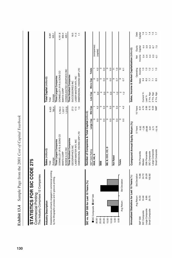
130
Exh
ibit
13.
4Sa
mpl
e Pa
ge f
rom
the
2001
Cos
t of C
apit
al Y
earb
ook
ST
AT
IST
ICS
FO
R S
IC C
OD
E 2
75C
omm
erci
alP
rintin
gT
his
Indu
stry
Com
pris
es 1
2 C
ompa
nies
Ind
ust
ry D
escr
ipti
on
Sal
es (
mill
ion$
)T
ota
l Cap
ital
(mill
ion$
)T
otal
Tot
al6,
061
Ave
rage
Ave
rage
505.
1
Th
ree
Lar
ges
t C
om
pan
ies
Th
ree
Lar
ges
t C
om
pan
ies
DO
NN
ELL
EY
(R
R)
& S
ON
S C
OD
ON
NE
LLE
Y (
R R
) &
SO
NS
CO
4,16
1.8
BA
NT
A C
OR
PB
AN
TA
CO
RP
830.
4
BO
WN
E &
CO
INC
CO
NS
OLI
DA
TE
D G
RA
PH
ICS
INC
429.
1
Th
ree
Sm
alle
st C
om
pan
ies
Th
ree
Sm
alle
st C
om
pan
ies
GE
OG
RA
PH
ICS
INC
27.3
S
UC
CE
SS
OR
IES
INC
18.5
LAS
ER
MA
ST
ER
INT
L IN
C17
.5
LAS
ER
MA
ST
ER
INT
L IN
C11
.5
DIM
EN
SIO
NA
L V
ISIO
NS
GR
P L
TD
1.0
D
IME
NS
ION
AL
VIS
ION
S G
RP
LT
D1.
1
SIC
vs.
S&
P 5
00 f
or
Las
t 10
Yea
rs (
%)
Nu
mb
er o
f C
om
pan
ies
& T
ota
l Cap
ital
(bi
llion
$)
S&
P D
ebt R
atin
gL
arg
e C
apM
id C
apL
ow
Cap
Mic
ro C
apT
ota
ls
AA
A, A
A, A
01
01
(com
pani
es)
0.0
4.2
0.0
4.2
(cap
ital)
BB
B0
00
0
0.0
0.0
0.0
0.0
BB
, B, C
CC
, CC
, D0
00
0
0.0
0.0
0.0
0.0
No
t R
ated
00
911
0.0
0.0
0.7
1.9
To
tals
01
912
0.0
4.2
0.7
6.1
An
nu
aliz
ed S
tati
stic
s fo
r L
ast
10 Y
ears
(%)
Co
mp
ou
nd
An
nu
al E
qu
ity
Ret
urn
(%
)S
ales
, In
com
e &
Mar
ket
Cap
ital
izat
ion
(bill
ion$
)
Avg
Ret
urn
Std
Dev
iatio
n5
Yea
rs10
Yea
rsO
pera
ting
Net
E
quity
Deb
t
S&
P 5
0015
.50
15.8
675
th P
erce
ntile
6.51
Sal
esIn
com
eIn
com
eC
apita
lC
apita
l
SIC
Com
posi
te10
.46
24.7
2M
edia
n4.
74C
urre
nt Y
r.9.
41.
31.
6
Larg
e C
ompo
site
8.85
25.2
925
th P
erce
ntile
2.85
Last
Yr.
8.2
1.3
1.7
Sm
all C
ompo
site
20.7
510
2.82
SIC
Com
posi
te6.
122
Yrs
. Ago
7.7
1.2
1.4
Larg
e C
ompo
site
6.03
3 Y
rs. A
go7.
11.
11.
5
Sm
all C
ompo
site
NM
F4
Yrs
. Ago
8.5
1.0
1.7
1,01
0.8
9,42
5
785.
4
5,
764.
3
1,53
7.7
0.71
-10.
16
6.02
-1.2
6
-29.
89
3.61
4.4
3.9
7.0
6.3
8.7
2
1.20
0.0 0
0.0 0
0.0 2
1.2
0.4
0.4
0.4
0.3
-0.1
Est
ablis
hmen
ts p
rimar
ily e
ngag
ed in
com
mer
cial
prin
ting
by th
e lit
hogr
aphi
c pr
oces
s an
d in
gra
vure
prin
ting.
0.00
5.00
10.0
0
15.0
0
20.0
0
25.0
0
30.0
0
Avg
Ret
urn
Std
Dev
iatio
n
SIC
Com
posi
teS
&P
500
3953 P-13 8/29/02 2:24 PM Page 130
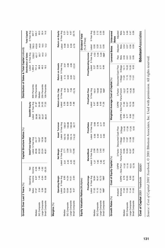
131
Sour
ce:
Cos
t of C
apit
al 2
001
Yea
rboo
k, ©
2001
Ibb
otso
n A
ssoc
iate
s, I
nc. U
sed
with
per
mis
sion
. All
righ
ts r
eser
ved.
Gro
wth
Ove
r L
ast
5 Y
ears
(%
)C
apit
al S
tru
ctu
re R
atio
s (%
)D
istr
ibu
tio
n o
f S
ales
& T
ota
l Cap
ital
(m
illio
n$)
Dis
trib
uti
on
of
Sal
esT
ota
l Cap
ital
Net
Ope
ratin
gN
etD
ebt/
To
tal C
apit
alD
ebt/
MV
Eq
uit
yLa
test
5-Y
ear
Avg
5-Y
ear
Avg
Sal
esIn
com
eIn
com
eLa
test
5-Y
ear
Avg
Late
st5-
Yea
r A
vg90
th P
erce
ntile
1,48
5.0
847.
7
Med
ian
17.9
76.
07-2
.26
28.5
624
.17
31.8
775
th P
erce
ntile
721.
453
5.1
SIC
Com
posi
te2.
541.
451.
8622
.22
19.6
724
.49
Med
ian
98.8
63.5
Larg
e C
ompo
site
0.99
-0.9
4-1
.62
23.2
419
.58
24.3
525
th P
erce
ntile
46.5
30.4
Sm
all C
ompo
site
19.0
89.
58-3
5.20
46.8
143
.68
77.5
510
th P
erce
ntile
18.5
14.6
Mar
gin
s(%
)
Op
erat
ing
Mar
gin
Net
Mar
gin
Ass
et T
urn
ove
rR
etu
rn o
n In
v. C
ap.
Ret
urn
on
Ass
ets
Ret
urn
on
Eq
uit
y
Late
st5-
Yea
r A
vgLa
test
5-Y
ear
Avg
Late
st5-
Yea
r A
vgLa
test
5-Y
ear
Avg
Late
st5-
Yea
r A
vg5-
Yea
r A
vg
Med
ian
10.0
48.
852.
715.
565.
31
SIC
Com
posi
te13
.64
14.3
43.
588.
094.
57
Larg
e C
ompo
site
13.4
414
.51
3.57
9.28
4.67
Sm
all C
ompo
site
6.57
-2.6
4-1
3.48
-1.8
8-2
2.75
Eq
uit
y V
alu
atio
n R
atio
s (M
ultip
les)
Div
iden
d Y
ield
(%
of P
rice)
Pri
ce/E
arn
ing
sM
arke
t/B
oo
k
P
rice
/Sal
es
P
rice
/Cas
h F
low
Pri
ce/O
per
atin
g In
com
e
Late
st5-
Yea
r A
vgLa
test
5-Y
ear
Avg
Late
st5-
Yea
r A
vgLa
test
5-Y
ear
Avg
Late
st5-
Yea
r A
vgLa
test
5-Y
ear
Avg
Med
ian
11.0
218
.84
2.08
9.47
3.27
0.00
0.00
SIC
Com
posi
te11
.10
16.4
72.
398.
663.
583.
202.
12
Larg
e C
ompo
site
11.9
115
.72
2.40
9.49
3.77
3.41
2.35
Sm
all C
ompo
site
NM
FN
MF
1.92
11.2
69.
990.
000.
00
Gro
wth
Rat
es (
%)
Co
st o
f E
qu
ity
Cap
ital
(%)
Wei
gh
ted
Ave
rag
e C
ost
of
Cap
ital
(%)
Lev
ered
Bet
asU
nle
vere
dB
etas
Ana
lyst
s'C
AP
M3-
Fac
tor
Dis
coun
ted
Cas
h F
low
CA
PM
3-F
acto
rD
isco
unte
d C
ash
Flo
w R
awA
djus
ted
Adj
uste
d
Est
imat
eC
AP
M+
Siz
e P
rem
Fam
a-F
renc
h1-
Sta
geC
AP
M+
Siz
e P
rem
Fam
a-F
renc
h1-
Sta
ge3-
Sta
ge B
eta
Bet
aB
eta
Med
ian
11.6
39.
7913
.96
11.6
39.
8011
.62
11.8
113
.11
0.55
0.54
0.27
SIC
Com
posi
te11
.63
10.0
315
.93
11.8
79.
7710
.57
11.1
515
.22
0.61
0.57
0.46
Larg
e C
ompo
site
11.4
49.
9315
.97
11.9
89.
6610
.10
11.2
215
.20
0.61
0.56
0.47
Sm
all C
ompo
site
11.6
310
.16
14.5
611
.63
11.0
212
.08
11.6
19.
530.
950.
590.
26
Co
st o
f C
apit
al 2
001
Yea
rboo
k©
2001
Ibb
ots
on
Ass
ocia
tes
10.5
112
.78
6.50
17.3
0
17.2
0
0.36
0.49
0.51
11.1
01.82
155.
14
114.
22
0.78
11.3
2
0.66
0.68
4.25
3-S
tage
14.4
0
0.59
0.77
3.97
4.86
Late
st
-0.7
6
138.
57
135.
88
136.
09
95.7
7
Late
st
7.08
4.86
-12.
91
8.39
9.08
790.
3
419.
8
44.9
18.5
9.01
12.2
12.8
0
-0.5
7
6.60
6.63
4.13
5.40
18.0
1
6.87
1.27
1.60
-15.
78
4.40
3.01
-0.5
0
150.
73
150.
83
0.70
14.2
6
39.9
8
28.5
7
30.2
7
88.0
1
19.6
9
NM
F
13.2
7
14.1
9
19.0
2
1228
.2
401.
7
83.7
5.28
NM
F
44.0
15.1
4.52
5.46
3953 P-13 8/29/02 2:24 PM Page 131
risk of an asset relative to the market and the return that can be expected from thatasset. The CAPM model determines the cost of equity for any company as equal tothe riskless rate plus an amount proportionate to its systematic risk. The formula is:
ki = rf + (bi × ERP)
where:
ki = The cost of equityrf = The riskless yieldbi = Beta of company iERP = Expected equity risk premium
The regression for each company is run over 60 months of total return data. AllCAPM models in the yearbook use the yield on a 20-year Treasury bond for the risk-less rate and the long-horizon equity risk premium for the equity risk premium. Val-ues for both the expected riskless rate and the expected equity risk premium (ERP) canbe found in the SBBI Valuation Edition Yearbook. The yearbook also provides indus-try betas that can be used to make modifications to the current CAPM assumptions.
The Cost of Capital Yearbook displays two CAPM-based cost of equity estimateswith identical OLS-adjusted betas; however, the second CAPM model incorporates asize premium. The size premium is included to account for the additional return pro-vided by small companies over large companies but not captured by the standardCAPM model (see the section on firm size premium for more information). For a par-ticular industry, the size premium is determined from the individual company size pre-mia, which are based on the equity capitalization of each company. (A size premium isadded only to mid-cap, low-cap, and micro-cap companies.) For composites, the sizepremium is an equity-capitalization-weighted average of the size premia of the compa-nies included in the industry.
When determining a cost of equity for an industry, the CAPM adjusted for sizebest represents the entire industry. The size adjustment for an industry dominated bylarge companies will be less than for an industry comprised mostly of small- or mid-cap companies. When valuing individual companies, however, it would be most ap-propriate to use the CAPM model that is not adjusted for size and instead add a sizepremium relative to the equity capitalization of the subject company. Full size premiumanalysis at the firm level is presented in the SBBI Valuation Edition Yearbook.
Fama-French Three-factor Model
The Fama-French three-factor model is a multiple linear regression model devel-oped by Eugene Fama and Kenneth French. The model is estimated by running a timeseries multiple regression for each company. The dependent variable is the company’smonthly excess returns over Treasury-bill returns. The independent variables are:
• The monthly excess return on the market over Treasury bills
• SMB (small minus big): The difference between the monthly return on small-capstocks and large-cap stocks
132 Estimating the Cost of Equity Capital
3953 P-13 8/29/02 2:24 PM Page 132
• HML (high minus low): The difference between monthly returns on high book-to-market stocks and low book-to-market stocks
The Fama-French three-factor model is shown in the next equation:
ki = rf + (bi × ERP) + (si × SMBP) + (hi × HMLP)
where:
ki = Cost of equity capital for company irf = The risk-free ratebi = Market coefficient in the Fama-French regressionERP = The expected equity risk premiumsi = Small-minus-big coefficient in the Fama-French regressionSMBP = The expected small-minus-big risk premium, estimated as the
difference between the historical average annual returns on thesmall-cap and large-cap portfolios
hi = High-minus-low coefficient in the Fama-French regressionHMLP = The expected high-minus-low risk premium, estimated as the
difference between the historical average annual returns on thehigh book-to-market and low book-to-market portfolios
The Fama-French three-factor model attempts to improve on the single-variableCAPM model by incorporating additional market variables to explain a company’sexpected return more adequately. These variables include the size of the companyand its book-to-market ratio (capturing the size effect and the financial distress of thefirm), in addition to the single-market variable of the CAPM. Because this model in-corporates more information into the cost of equity estimate than the typical CAPM,estimates on average tend to be higher.
Discounted Cash Flow Models
The discounted cash flow model (DCF), or income approach, was developed byJohn Burr Williams and elaborated by Myron J. Gordan and Eli Shapiro. The idea be-hind the DCF model is that the present value of a company can be estimated by dis-counting its dividends or expected cash flows using the firm’s appropriate discountrate. Therefore, the set of inputs needed to determine a company’s present value in-clude the value of future cash flows, the rate at which these cash flows will grow, andthe discount rate that will equate future cash flows to their present value. Alternatively,given these inputs, we can use the DCF model to solve for the discount rate or thecost of equity.
Assuming that the present value of a company and its projected cash flows areknown, there still exists the difficulty of obtaining a cash flow growth forecast, sincecash flows tend not to grow at a constant rate forever. In this case, the yearbook usesthe expected earning growth rates from the I/B/E/S database of consensus long-termgrowth rate estimates.
Using Ibbotson Associates Cost of Capital Data 133
3953 P-13 8/29/02 2:24 PM Page 133
The one-stage and three-stage discounted cash flow models presented in theCost of Capital Yearbook are both rooted in the Gordon Growth Model, which is:
Pi = D / (ki – gi)
where:
Pi = The price per share for company iDi = The dividend per share for company i at the end of year 1ki = The discount rate for company igi = The dividend growth rate for company i
To solve for the cost of equity capital, the formula is rewritten as:
ki = {[Di × (1 + g)]/Pi} + gi
The single-stage growth model describes the cost of equity capital for a companythat has a constant expected cash flow growth rate projected indefinitely into the fu-ture. One drawback of the single-stage model is that if a company pays no dividends,its cost of equity is equivalent to its growth rate. Given such shortcomings, the prac-titioner must recognize the limitations of the model on its own and view the resultsas a point of comparison with other models in estimating the cost of equity.
It is probably unrealistic to assume that a firm’s cash flows will grow at a con-stant rate in perpetuity. To improve the predictability of the DCF cost of equitymodel, a more realistic assumption might be that the growth rate of cash flows changesover time. The three-stage DCF model estimates the cost of equity employing threedifferent growth rate estimates at different future time periods. The Cost of CapitalYearbook calculates the three-stage DCF cost of equity for each industry assumingthat cash flows will grow at the analyst’s company-specific rates for the first five years,at an industry-average growth rate for the next five years, and finally at a growth ratefor the entire economy (expected real growth rate plus an inflation estimate) for allother time periods. The results of each model are shown in the bottom section ofExhibit 13.4.
IBBOTSON BETA BOOK
The Ibbotson Beta Book, published semiannually, includes company-specific betasfor more than 5,000 companies. Company betas are calculated for the ordinary leastsquares (OLS) CAPM and Fama-French model with regression factors. A samplepage from the Beta Book can be seen in Exhibit 13.5.
The Beta Book does not provide cost of equity estimates for individual compa-nies; however, it does provide practitioners with the statistics necessary for calculat-ing cost of equity under both the Capital Asset Pricing Model and the three-factormodel described by Fama and French.
134 Estimating the Cost of Equity Capital
3953 P-13 8/29/02 2:24 PM Page 134
Those companies included in the Beta Book are selected from the COMPUSTATdatabase based on three criteria:
1. A company must have at least 36 months of return data available.
2. It must have sales greater than $100,000 in the most recent year.
3. It must have a market capitalization greater than $10,000 for the most recentmonth.
Beta Estimation Methodologies
For the CAPM model, the Ibbotson Beta Book provides several equity beta sta-tistics including traditional unlevered and levered ordinary least squares beta esti-mates, peer group betas, and Ibbotson adjusted betas. For the Fama-French model, thebeta factor in addition to size and value factors identified in the model are provided.
All CAPM regressions in the Beta Book are run over a 60-month period, usingthe S&P 500 total returns as a proxy for the market returns and the yield on a 30-dayTreasury bill as a proxy for the risk-free asset. If a company has less than 60 monthsof historical returns, then betas are calculated using its available return data with aminimum of 36 months being acceptable.
Please refer to the “Cost of Capital Yearbook” section of this chapter for detailedinformation about the CAPM and Fama-French models.
Levered and Unlevered Betas
The OLS CAPM results for each company include both levered and unleveredbetas. Whereas the levered beta incorporates both the business and financing risks un-dertaken by the company and borne by the equity shareholders, the unlevered beta ex-cludes the risk implicit in the financial structure of a company and only reflects itsbusiness risk. This allows a practitioner to make adjustments to the capital structureinherent in a levered beta by relevering a company’s unlevered beta with a debt struc-ture more similar to the subject company being valued. The unlevered beta is alsouseful when it may be difficult to make comparisons within an industry for a com-pany that has much higher leverage than its peers. In this case, because the unleveredbeta reflects only business risk and not financial risk, the practitioner could releverthe company’s beta with that of its industry to make a more comparable peer groupanalysis.
Ibbotson (Adjusted) Betas
The Beta Book includes an adjusted or forward-looking beta for each of the CAPMmodels. The adjustment incorporates the theory that a company’s beta tends to reverttoward its industry’s average beta over time. The adjusted beta is calculated using the
Using Ibbotson Associates Cost of Capital Data 135
3953 P-13 8/29/02 2:24 PM Page 135
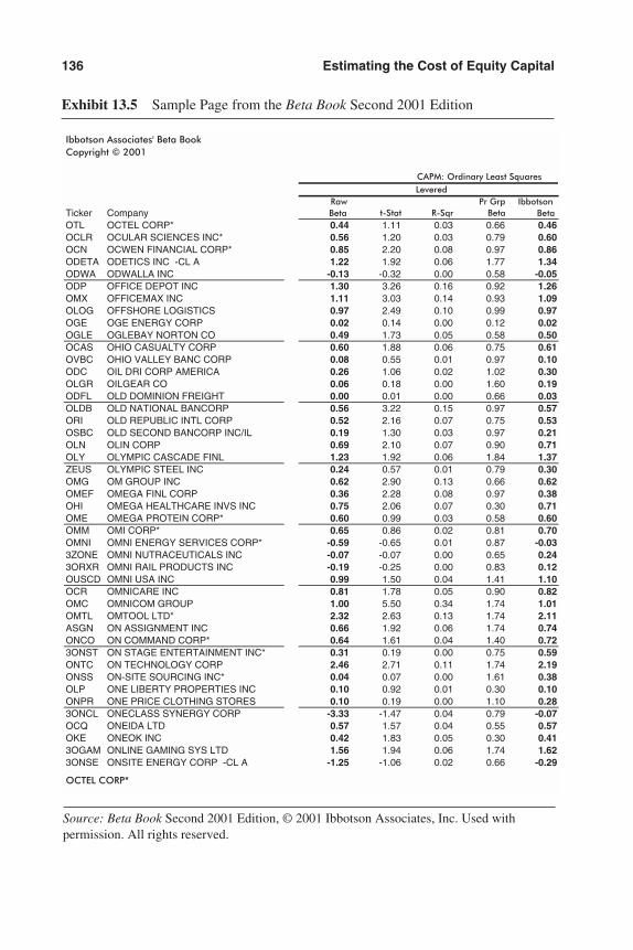
136 Estimating the Cost of Equity Capital
Exhibit 13.5 Sample Page from the Beta Book Second 2001 Edition
CAPM: Ordinary Least SquaresLevered
Ticker CompanyRawBeta t-Stat R-Sqr
Pr Grp Beta
IbbotsonBeta
OTL OCTEL CORP* 0.44 1.11 0.03 0.66 0.46OCLR OCULAR SCIENCES INC* 0.56 1.20 0.03 0.79 0.60OCN OCWEN FINANCIAL CORP* 0.85 2.20 0.08 0.97 0.86ODETA ODETICS INC -CL A 1.22 1.92 0.06 1.77 1.34ODWA ODWALLA INC -0.13 -0.32 0.00 0.58 -0.05ODP OFFICE DEPOT INC 1.30 3.26 0.16 0.92 1.26OMX OFFICEMAX INC 1.11 3.03 0.14 0.93 1.09OLOG OFFSHORE LOGISTICS 0.97 2.49 0.10 0.99 0.97OGE OGE ENERGY CORP 0.02 0.14 0.00 0.12 0.02OGLE OGLEBAY NORTON CO 0.49 1.73 0.05 0.58 0.50OCAS OHIO CASUALTY CORP 0.60 1.88 0.06 0.75 0.61OVBC OHIO VALLEY BANC CORP 0.08 0.55 0.01 0.97 0.10ODC OIL DRI CORP AMERICA 0.26 1.06 0.02 1.02 0.30OLGR OILGEAR CO 0.06 0.18 0.00 1.60 0.19ODFL OLD DOMINION FREIGHT 0.00 0.01 0.00 0.66 0.03OLDB OLD NATIONAL BANCORP 0.56 3.22 0.15 0.97 0.57ORI OLD REPUBLIC INTL CORP 0.52 2.16 0.07 0.75 0.53OSBC OLD SECOND BANCORP INC/IL 0.19 1.30 0.03 0.97 0.21OLN OLIN CORP 0.69 2.10 0.07 0.90 0.71OLY OLYMPIC CASCADE FINL 1.23 1.92 0.06 1.84 1.37ZEUS OLYMPIC STEEL INC 0.24 0.57 0.01 0.79 0.30OMG OM GROUP INC 0.62 2.90 0.13 0.66 0.62OMEF OMEGA FINL CORP 0.36 2.28 0.08 0.97 0.38OHI OMEGA HEALTHCARE INVS INC 0.75 2.06 0.07 0.30 0.71OME OMEGA PROTEIN CORP* 0.60 0.99 0.03 0.58 0.60OMM OMI CORP* 0.65 0.86 0.02 0.81 0.70OMNI OMNI ENERGY SERVICES CORP* -0.59 -0.65 0.01 0.87 -0.033ZONE OMNI NUTRACEUTICALS INC -0.07 -0.07 0.00 0.65 0.243ORXR OMNI RAIL PRODUCTS INC -0.19 -0.25 0.00 0.83 0.12OUSCD OMNI USA INC 0.99 1.50 0.04 1.41 1.10OCR OMNICARE INC 0.81 1.78 0.05 0.90 0.82OMC OMNICOM GROUP 1.00 5.50 0.34 1.74 1.01OMTL OMTOOL LTD* 2.32 2.63 0.13 1.74 2.11ASGN ON ASSIGNMENT INC 0.66 1.92 0.06 1.74 0.74ONCO ON COMMAND CORP* 0.64 1.61 0.04 1.40 0.723ONST ON STAGE ENTERTAINMENT INC* 0.31 0.19 0.00 0.75 0.59ONTC ON TECHNOLOGY CORP 2.46 2.71 0.11 1.74 2.19ONSS ON-SITE SOURCING INC* 0.04 0.07 0.00 1.61 0.38OLP ONE LIBERTY PROPERTIES INC 0.10 0.92 0.01 0.30 0.10ONPR ONE PRICE CLOTHING STORES 0.10 0.19 0.00 1.10 0.283ONCL ONECLASS SYNERGY CORP -3.33 -1.47 0.04 0.79 -0.07OCQ ONEIDA LTD 0.57 1.57 0.04 0.55 0.57OKE ONEOK INC 0.42 1.83 0.05 0.30 0.413OGAM ONLINE GAMING SYS LTD 1.56 1.94 0.06 1.74 1.623ONSE ONSITE ENERGY CORP -CL A -1.25 -1.06 0.02 0.66 -0.29
OCTEL CORP*
Ibbotson Associates' Beta BookCopyright © 2001
Source: Beta Book Second 2001 Edition, © 2001 Ibbotson Associates, Inc. Used withpermission. All rights reserved.
3953 P-13 8/29/02 2:24 PM Page 136
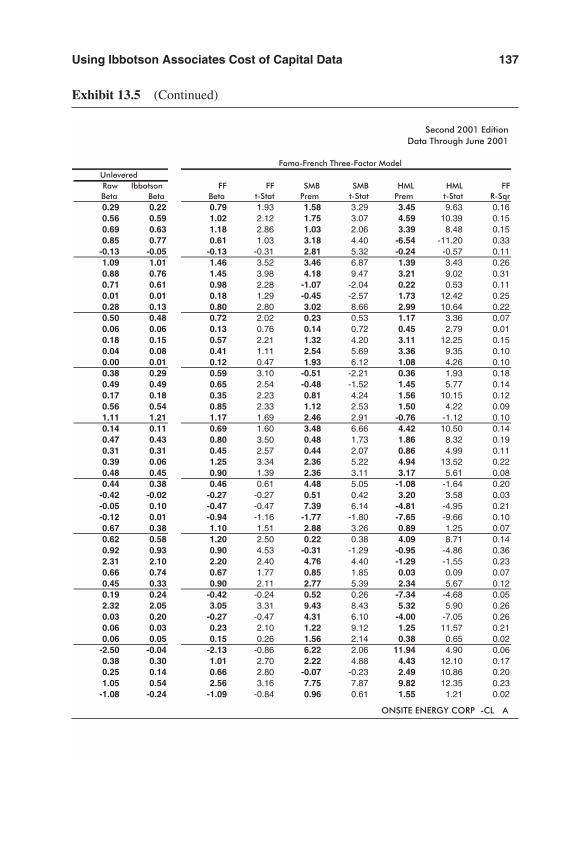
Using Ibbotson Associates Cost of Capital Data 137
Exhibit 13.5 (Continued)
Fama-French Three-Factor ModelUnleveredRawBeta
IbbotsonBeta
FFBeta
FFt-Stat
SMBPrem
SMBt-Stat
HMLPrem
HMLt-Stat
FFR-Sqr
0.29 0.22 0.79 1.93 1.58 3.29 3.45 9.63 0.160.56 0.59 1.02 2.12 1.75 3.07 4.59 10.39 0.150.69 0.63 1.18 2.86 1.03 2.06 3.39 8.48 0.150.85 0.77 0.61 1.03 3.18 4.40 -6.54 -11.20 0.33
-0.13 -0.05 -0.13 -0.31 2.81 5.32 -0.24 -0.57 0.111.09 1.01 1.46 3.52 3.46 6.87 1.39 3.43 0.260.88 0.76 1.45 3.98 4.18 9.47 3.21 9.02 0.310.71 0.61 0.98 2.28 -1.07 -2.04 0.22 0.53 0.110.01 0.01 0.18 1.29 -0.45 -2.57 1.73 12.42 0.250.28 0.13 0.80 2.80 3.02 8.66 2.99 10.64 0.220.50 0.48 0.72 2.02 0.23 0.53 1.17 3.36 0.070.06 0.06 0.13 0.76 0.14 0.72 0.45 2.79 0.010.18 0.15 0.57 2.21 1.32 4.20 3.11 12.25 0.150.04 0.08 0.41 1.11 2.54 5.69 3.36 9.35 0.100.00 0.01 0.12 0.47 1.93 6.12 1.08 4.26 0.100.38 0.29 0.59 3.10 -0.51 -2.21 0.36 1.93 0.180.49 0.49 0.65 2.54 -0.48 -1.52 1.45 5.77 0.140.17 0.18 0.35 2.23 0.81 4.24 1.56 10.15 0.120.56 0.54 0.85 2.33 1.12 2.53 1.50 4.22 0.091.11 1.21 1.17 1.69 2.46 2.91 -0.76 -1.12 0.100.14 0.11 0.69 1.60 3.48 6.66 4.42 10.50 0.140.47 0.43 0.80 3.50 0.48 1.73 1.86 8.32 0.190.31 0.31 0.45 2.57 0.44 2.07 0.86 4.99 0.110.39 0.06 1.25 3.34 2.36 5.22 4.94 13.52 0.220.48 0.45 0.90 1.39 2.36 3.11 3.17 5.61 0.080.44 0.38 0.46 0.61 4.48 5.05 -1.08 -1.64 0.20
-0.42 -0.02 -0.27 -0.27 0.51 0.42 3.20 3.58 0.03-0.05 0.10 -0.47 -0.47 7.39 6.14 -4.81 -4.95 0.21-0.12 0.01 -0.94 -1.16 -1.77 -1.80 -7.65 -9.66 0.100.67 0.38 1.10 1.51 2.88 3.26 0.89 1.25 0.070.62 0.58 1.20 2.50 0.22 0.38 4.09 8.71 0.140.92 0.93 0.90 4.53 -0.31 -1.29 -0.95 -4.86 0.362.31 2.10 2.20 2.40 4.76 4.40 -1.29 -1.55 0.230.66 0.74 0.67 1.77 0.85 1.85 0.03 0.09 0.070.45 0.33 0.90 2.11 2.77 5.39 2.34 5.67 0.120.19 0.24 -0.42 -0.24 0.52 0.26 -7.34 -4.68 0.052.32 2.05 3.05 3.31 9.43 8.43 5.32 5.90 0.260.03 0.20 -0.27 -0.47 4.31 6.10 -4.00 -7.05 0.260.06 0.03 0.23 2.10 1.22 9.12 1.25 11.57 0.210.06 0.05 0.15 0.26 1.56 2.14 0.38 0.65 0.02
-2.50 -0.04 -2.13 -0.86 6.22 2.06 11.94 4.90 0.060.38 0.30 1.01 2.70 2.22 4.88 4.43 12.10 0.170.25 0.14 0.66 2.80 -0.07 -0.23 2.49 10.86 0.201.05 0.54 2.56 3.16 7.75 7.87 9.82 12.35 0.23
-1.08 -0.24 -1.09 -0.84 0.96 0.61 1.55 1.21 0.02
ONSITE ENERGY CORP -CL A
Second 2001 EditionData Through June 2001
3953 P-13 8/29/02 2:24 PM Page 137
Vasicek Shrinkage Technique, which takes the statistically weighted average of thecompany beta and the industry beta. The formula is:
Adjusted Beta = (1 – weight) × peer group beta + weight × company beta
where,
Weight = (cross-sectional standard error)2/[(cross-sectional standarderror)2 + (time series beta standard error)2]
The Vasicek adjustment focuses on the statistical significance of the beta esti-mate, using the standard error to appropriately weight the company and industry beta.If the historical company beta displays low statistical significance, the higher standarderror will result in the company’s having a lower weighting than the industry, and viceversa. The greater the statistical confidence of the company’s regression beta, the closerthat weight is to 1.0.
The motivation behind adjusting a beta is to calculate a forward-looking estimatefrom a historical beta. An advantage of the Vasicek technique is that the adjustmentdoes not need to be made toward the market as a whole but can be made toward an in-dustry or a peer group. Also, if a company’s beta estimate seems statistically unreliable,confidence in the prospective beta can be increased by assigning a greater weight to itsindustry or peer group.
Peer Group and Industry Betas
In addition to individual company raw and adjusted betas, the Ibbotson Beta Bookalso provides peer group betas. Peer group betas are calculated by taking the sales-weighted average of the betas for each industry in which a company has sales. Thesebetas can be useful for comparison purposes or in place of a company beta display-ing poor regression statistics.
The Beta Book includes OLS betas for industries defined by two-digit SIC codes.Previous versions of the publication constructed each industry beta using the market-capitalization-weighted average of the betas of all companies in the industry. Onlycompanies with 75% of their sales in the industry as defined by the primary SIC codesof its business segments were included. However, this “pure play” approach tends toexclude many domestic conglomerates that are major participants in the industry.
In order to calculate an industry beta using data from all companies participatingin a particular industry, the Beta Book uses the Full Information Beta proceduredeveloped by Paul Kaplan and James Peterson. In this procedure, a single market-capitalization-weighted cross-sectional regression is performed using individualcompany betas as the dependent variable and the percentage of exposure or sales tothe industry as the independent variables. The resulting regression coefficients foreach industry are the estimates of the pure-play industry betas for which data fromevery company in a particular industry has been incorporated.
138 Estimating the Cost of Equity Capital
3953 P-13 8/29/02 2:24 PM Page 138
COST OF CAPITAL CENTER
The Cost of Capital Center at www.ibbotson.com is a Web site devoted to businessvaluation issues. As the name suggests, this site is the center of all things cost of cap-ital. The site offers analysis on more than 300 industries, 5,000 companies, and 145countries.
Ibbotson Associates uses the Cost of Capital Center as an outlet for much of itsvaluation-related data. Visitors to the site can purchase data from the Cost of CapitalYearbook and the Beta Book on a per-usage basis. Anyone interested in internationalcost of capital analysis will find the collection of international reports at the site crit-ical in calculations. The Cost of Capital Center is segmented into four main productgroups:
1. Industry Analysis
2. Company Analysis
3. Global Analysis
4. Risk Premia
Industry analysis available at the Cost of Capital Center is taken directly from theCost of Capital Yearbook published by Ibbotson Associates. Industries are organized bySIC code and are available for immediate download at the site. Ibbotson presents in-dustry analysis on more than 300 industries and updates the data at the Web site quar-terly. Included in the analysis are multiple measures of cost of equity, WACC, beta,capital structure ratios, growth rates, industry multiples, and other important financialstatistics. (See the section on the Cost of Capital Yearbook for more information.)
Company analysis presented on the Web site includes individual company betasand tax rates. Over 5,000 company betas are taken directly from Ibbotson’s Beta Bookand sold at the site on a per-company basis. For each company, multiple measures ofbeta are displayed, including levered and unlevered betas, betas adjusted toward theirpeer group, and statistics necessary to calculate Fama-French three-factor cost of eq-uity. (See the section on the Beta Book for more information.) In addition to betaanalysis at the company level, Ibbotson also presents tax rate estimates. Research hasshown that using the top marginal tax rate in cost of capital calculations may be over-stating the effect of taxes. Ibbotson provides tax rate estimates on more than 5,000companies that can be used in discounting projected future cash flows. Tax rate esti-mates based on the most recent fiscal year and the five-year average are presented foreach company. Company betas are updated on the Web site quarterly, while companytax rates are updated annually (usually in the fall).
The remaining sections of the Web site present data reports for global analysisand risk premia analysis. The global analysis section provides equity risk premia andcost of equity estimates for a variety of countries. The International Equity Risk Pre-mia Report provides ERP estimates on 16 different developed countries. The analy-sis can be customized to view the ERP for any time period covered for each country.When available, data are presented for both the long- and short-horizon ERP, in both
Using Ibbotson Associates Cost of Capital Data 139
3953 P-13 8/29/02 2:24 PM Page 139
U.S. dollars and local currency. Most of the ERP estimates use a historical date rangethat extends back to 1970. Using a longer string of data, Ibbotson is also able to pro-vide a Canadian Risk Premia over Time Report and a United Kingdom Risk Premiaover Time Report.
Some of the most popular reports available on the Web site are the InternationalCost of Capital Report and the International Cost of Capital Perspectives Report.The first presents cost of equity estimates on approximately 145 countries from theperspective of U.S. investors. This report offers estimates using up to five differentcost of equity models for each country, based on data availability. The “perspectives”report also covers 145 countries but from the perspective of international investors.This report utilizes only one model for cost of equity estimation (the country risk rat-ing model) and presents the estimates from the perspective of investors in Australia,Canada, France, Germany, Japan, and the United Kingdom. Examples of the data of-fered in both reports can be seen in Exhibits 13.6 and 13.7. All international reportsare updated annually on the Web site.
In addition to the international reports available at the Cost of Capital Center, anumber of U.S.-based risk premium reports are presented: specifically, the Risk Pre-mia over Time Report and the Standard & Poor’s Corporate Value Consulting RiskPremium Report (formerly the PricewaterhouseCoopers Risk Premium Study). TheRisk Premia over Time Report provides equity and size premia over all historical timeperiods dating back to 1926. The analysis can be customized by choosing the begin-ning and ending date for risk premia estimation. The report contains long-, interme-diate- and short-term equity risk premia and mid-, low- and micro-cap size premia.All of the content in this report is from the SBBI Valuation Edition Yearbook, pri-marily from Appendix A. The Standard & Poor’s Corporate Value Consulting RiskPremium Report (formerly the PricewaterhouseCoopers Risk Premium Study) iswritten by Roger Grabowski and David King, currently with Standard & Poor’s Cor-porate Value Consulting, formerly of PricewaterhouseCoopers. Companies are di-vided into 25 different size groups based on:
• Market value of equity
• Book value of equity
• Five-year average net income
• Market value of invested capital
• Total assets
• Five-year average EBITDA
• Sales
• Number of employees
140 Estimating the Cost of Equity Capital
3953 P-13 8/29/02 2:24 PM Page 140
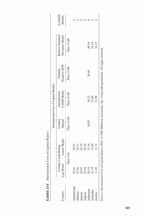
141
Exh
ibit
13.
6In
tern
atio
nal C
ost o
f Cap
ital
Rep
ort
Inte
rnat
iona
l Cos
t of
Cap
ital M
odel
s
Cou
ntry
Cre
dit R
atin
gC
ount
ryIn
tern
atio
nal
Glo
bally
Rel
ativ
e St
anda
rdA
vaila
ble
Cou
ntry
Log
Mod
elL
inea
r M
odel
Spre
adC
APM
Mod
elN
este
d C
APM
Dev
iatio
n M
odel
Mod
els
Thr
u 3-
01T
hru
12-0
0T
hru
12-0
0T
hru
12-0
0T
hru
12-0
0
Afg
hani
stan
47.6
130
.53
2A
lban
ia35
.20
28.3
12
Alg
eria
24.8
724
.19
2A
ngol
a39
.16
29.2
42
Arg
entin
a20
.34
21.1
619
.92
16.2
230
.49
49.3
96
Aus
tral
ia12
.19
12.5
013
.09
18.1
44
Aus
tria
11.3
611
.31
11.9
016
.15
4
Sour
ce:
Inte
rnat
iona
l Cos
t of C
apit
al R
epor
t 200
1, ©
2001
Ibb
otso
n A
ssoc
iate
s, I
nc. U
sed
with
per
mis
sion
. All
righ
ts r
eser
ved.
3953 P-13 8/29/02 2:24 PM Page 141
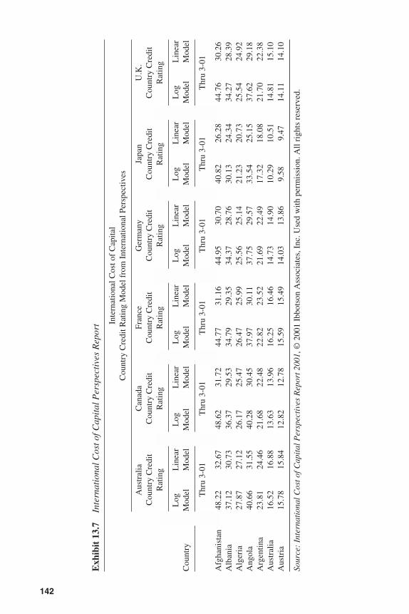
142
Exh
ibit
13.
7In
tern
atio
nal C
ost o
f Cap
ital
Per
spec
tive
s R
epor
t Inte
rnat
iona
l Cos
t of
Cap
ital
Cou
ntry
Cre
dit R
atin
g M
odel
fro
m I
nter
natio
nal P
ersp
ectiv
es
Aus
tral
iaC
anad
aFr
ance
Ger
man
yJa
pan
U.K
.C
ount
ry C
redi
tC
ount
ry C
redi
tC
ount
ry C
redi
tC
ount
ry C
redi
tC
ount
ry C
redi
tC
ount
ry C
redi
tR
atin
gR
atin
gR
atin
gR
atin
gR
atin
gR
atin
g
Log
Lin
ear
Log
Lin
ear
Log
Lin
ear
Log
Lin
ear
Log
Lin
ear
Log
Lin
ear
Cou
ntry
Mod
elM
odel
Mod
elM
odel
Mod
elM
odel
Mod
elM
odel
Mod
elM
odel
Mod
elM
odel
Thr
u 3-
01T
hru
3-01
Thr
u 3-
01T
hru
3-01
Thr
u 3-
01T
hru
3-01
Afg
hani
stan
48.2
232
.67
48.6
231
.72
44.7
731
.16
44.9
530
.70
40.8
226
.28
44.7
630
.26
Alb
ania
37.1
230
.73
36.3
729
.53
34.7
929
.35
34.3
728
.76
30.1
324
.34
34.2
728
.39
Alg
eria
27.8
727
.12
26.1
725
.47
26.4
725
.99
25.5
625
.14
21.2
320
.73
25.5
424
.92
Ang
ola
40.6
631
.55
40.2
830
.45
37.9
730
.11
37.7
529
.57
33.5
425
.15
37.6
229
.18
Arg
entin
a23
.81
24.4
621
.68
22.4
822
.82
23.5
221
.69
22.4
917
.32
18.0
821
.70
22.3
8A
ustr
alia
16.5
216
.88
13.6
313
.96
16.2
516
.46
14.7
314
.90
10.2
910
.51
14.8
115
.10
Aus
tria
15.7
815
.84
12.8
212
.78
15.5
915
.49
14.0
313
.86
9.58
9.47
14.1
114
.10
Sour
ce:
Inte
rnat
iona
l Cos
t of C
apit
al P
ersp
ecti
ves
Rep
ort 2
001,
©20
01 I
bbot
son
Ass
ocia
tes,
Inc
. Use
d w
ith p
erm
issi
on. A
ll ri
ghts
res
erve
d.
3953 P-13 8/29/02 2:24 PM Page 142
143
Chapter 14
Arbitrage Pricing ModelExplanation of the APT ModelAPM FormulaSummary
The concept of the arbitrage pricing theory (APT) was introduced by academi-cians in 1976.1 However, it was not until 1988 that data in a commercially usableform became generally available to permit the application of the theory to the estima-tion of required rates of return in day-to-day practice. Despite the theory’s longevity,it still is not widely used by practitioners today.
EXPLANATION OF THE APT MODEL
As noted in Chapter 9, the Capital Asset Pricing Model (CAPM) is a univariatemodel; that is, CAPM recognizes only one risk factor—systematic risk relative to amarket index. In a sense, APT is a multivariate extension of the CAPM. APT recog-nizes a variety of risk factors that may bear pervasively on an investment’s requiredrate of return, one of which may be a CAPM-type “market” or “market timing” risk.It may be argued that the CAPM and APT are not mutually exclusive, nor is one ofgreater or lesser scope than the other. It also can be argued that the CAPM beta im-plicitly reflects the information included separately in each of the APT “factors.”However, in spite of its more limited use, most academicians consider the arbitragepricing model (APM) richer in its information content and explanatory and predictivepower.
Whereas the nature of the CAPM is a single regression, the nature of the APMis a multiple regression. In the APM, the cost of capital for an investment varies ac-cording to that investment’s sensitivity to each of several different risk factors.
The model itself does not specify what the risk factors are. Most formulations ofthe APM consider only risk factors of a pervasive macroeconomic nature, such as:
• Yield spread. The differential between risky and less risky bonds as a measure ofinvestors’ consensus confidence in economic prosperity
• Interest rate risk. Measured by the difference between long-term and short-termyields
3953 P-14 8/29/02 2:24 PM Page 143
• Business outlook risk. Measured by changes in forecasts for economic variablessuch as gross national product (GNP)
• Inflation risk. Measured by changes in inflation forecasts
The beta used in the CAPM may or may not be one of the risk factors includedin any particular practitioner’s version of the APM. In some versions, more industry-specific factors may be included, such as changes in oil prices. Exhibit 14.1 explainsone version of APT risk factors.
APM FORMULA
The econometric estimation of the arbitrage pricing model with multiple risk fac-tors yields this formula:
Formula 14.1
E(Ri) = Rf + (Bi1K1) + (Bi2K2) + … + (BinKn)
where:
E(Ri) = Expected rate of return on the subject securityRf = Rate of return on a risk-free securityK1 … Kn = Risk premium associated with factor K for the average asset
in the marketBi1 … Bin = Sensitivity of security i to each risk factor relative to the
market average sensitivity to that factor
Roger Ibbotson and Gary Brinson make the following observations regardingAPT:
In theory, a specific asset has some number of units of each risk; those units are eachmultiplied by the appropriate risk premium. Thus, APT shows that the equilibrium ex-pected return is the risk-free rate plus the sum of a series of risk premiums. APT is morerealistic than CAPM because investors can consider other characteristics besides thebeta of assets as they select their investment portfolios.2
Research has shown that the cost of equity capital as estimated by the APM tendsto be higher for some industries (e.g., oil) and lower for others (e.g., certain utilitygroups) than the cost of equity capital using the CAPM. Early research also suggeststhat the multivariate APT model explains expected rates of return better than does theunivariate CAPM.3
So, if the APM is more powerful than the CAPM, why is the APM not used more?For one thing, the variables are not specified. Also, there is no universal consensusabout which variables are likely to have the greatest efficacy. Furthermore, the APM iscomplicated in that coefficients for several factors, rather than just one factor, must beworked out for each company for each specific time it is going to be applied.
144 Estimating the Cost of Equity Capital
3953 P-14 8/29/02 2:24 PM Page 144
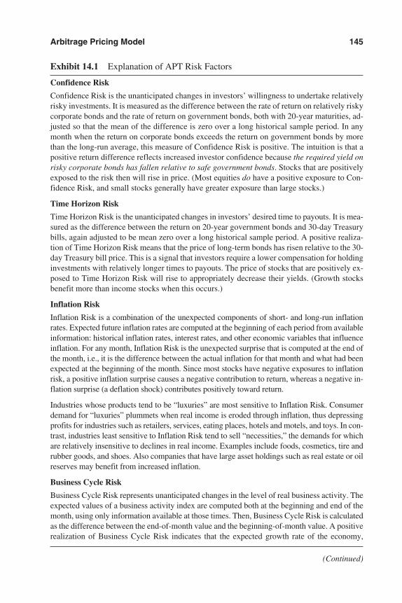
Arbitrage Pricing Model 145
Exhibit 14.1 Explanation of APT Risk Factors
Confidence Risk
Confidence Risk is the unanticipated changes in investors’ willingness to undertake relativelyrisky investments. It is measured as the difference between the rate of return on relatively riskycorporate bonds and the rate of return on government bonds, both with 20-year maturities, ad-justed so that the mean of the difference is zero over a long historical sample period. In anymonth when the return on corporate bonds exceeds the return on government bonds by morethan the long-run average, this measure of Confidence Risk is positive. The intuition is that apositive return difference reflects increased investor confidence because the required yield onrisky corporate bonds has fallen relative to safe government bonds. Stocks that are positivelyexposed to the risk then will rise in price. (Most equities do have a positive exposure to Con-fidence Risk, and small stocks generally have greater exposure than large stocks.)
Time Horizon Risk
Time Horizon Risk is the unanticipated changes in investors’ desired time to payouts. It is mea-sured as the difference between the return on 20-year government bonds and 30-day Treasurybills, again adjusted to be mean zero over a long historical sample period. A positive realiza-tion of Time Horizon Risk means that the price of long-term bonds has risen relative to the 30-day Treasury bill price. This is a signal that investors require a lower compensation for holdinginvestments with relatively longer times to payouts. The price of stocks that are positively ex-posed to Time Horizon Risk will rise to appropriately decrease their yields. (Growth stocksbenefit more than income stocks when this occurs.)
Inflation Risk
Inflation Risk is a combination of the unexpected components of short- and long-run inflationrates. Expected future inflation rates are computed at the beginning of each period from availableinformation: historical inflation rates, interest rates, and other economic variables that influenceinflation. For any month, Inflation Risk is the unexpected surprise that is computed at the end ofthe month, i.e., it is the difference between the actual inflation for that month and what had beenexpected at the beginning of the month. Since most stocks have negative exposures to inflationrisk, a positive inflation surprise causes a negative contribution to return, whereas a negative in-flation surprise (a deflation shock) contributes positively toward return.
Industries whose products tend to be “luxuries” are most sensitive to Inflation Risk. Consumerdemand for “luxuries” plummets when real income is eroded through inflation, thus depressingprofits for industries such as retailers, services, eating places, hotels and motels, and toys. In con-trast, industries least sensitive to Inflation Risk tend to sell “necessities,” the demands for whichare relatively insensitive to declines in real income. Examples include foods, cosmetics, tire andrubber goods, and shoes. Also companies that have large asset holdings such as real estate or oilreserves may benefit from increased inflation.
Business Cycle Risk
Business Cycle Risk represents unanticipated changes in the level of real business activity. Theexpected values of a business activity index are computed both at the beginning and end of themonth, using only information available at those times. Then, Business Cycle Risk is calculatedas the difference between the end-of-month value and the beginning-of-month value. A positiverealization of Business Cycle Risk indicates that the expected growth rate of the economy,
(Continued)
3953 P-14 8/29/02 2:24 PM Page 145
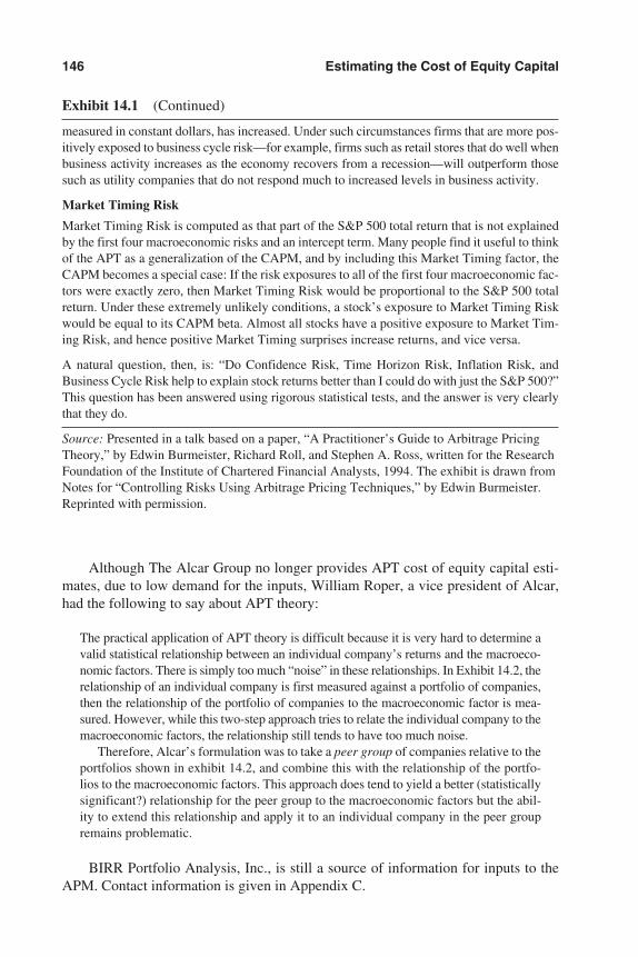
Although The Alcar Group no longer provides APT cost of equity capital esti-mates, due to low demand for the inputs, William Roper, a vice president of Alcar,had the following to say about APT theory:
The practical application of APT theory is difficult because it is very hard to determine avalid statistical relationship between an individual company’s returns and the macroeco-nomic factors. There is simply too much “noise” in these relationships. In Exhibit 14.2, therelationship of an individual company is first measured against a portfolio of companies,then the relationship of the portfolio of companies to the macroeconomic factor is mea-sured. However, while this two-step approach tries to relate the individual company to themacroeconomic factors, the relationship still tends to have too much noise.
Therefore, Alcar’s formulation was to take a peer group of companies relative to theportfolios shown in exhibit 14.2, and combine this with the relationship of the portfo-lios to the macroeconomic factors. This approach does tend to yield a better (statisticallysignificant?) relationship for the peer group to the macroeconomic factors but the abil-ity to extend this relationship and apply it to an individual company in the peer groupremains problematic.
BIRR Portfolio Analysis, Inc., is still a source of information for inputs to theAPM. Contact information is given in Appendix C.
146 Estimating the Cost of Equity Capital
Exhibit 14.1 (Continued)
measured in constant dollars, has increased. Under such circumstances firms that are more pos-itively exposed to business cycle risk—for example, firms such as retail stores that do well whenbusiness activity increases as the economy recovers from a recession—will outperform thosesuch as utility companies that do not respond much to increased levels in business activity.
Market Timing Risk
Market Timing Risk is computed as that part of the S&P 500 total return that is not explainedby the first four macroeconomic risks and an intercept term. Many people find it useful to thinkof the APT as a generalization of the CAPM, and by including this Market Timing factor, theCAPM becomes a special case: If the risk exposures to all of the first four macroeconomic fac-tors were exactly zero, then Market Timing Risk would be proportional to the S&P 500 totalreturn. Under these extremely unlikely conditions, a stock’s exposure to Market Timing Riskwould be equal to its CAPM beta. Almost all stocks have a positive exposure to Market Tim-ing Risk, and hence positive Market Timing surprises increase returns, and vice versa.
A natural question, then, is: “Do Confidence Risk, Time Horizon Risk, Inflation Risk, andBusiness Cycle Risk help to explain stock returns better than I could do with just the S&P 500?”This question has been answered using rigorous statistical tests, and the answer is very clearlythat they do.
Source: Presented in a talk based on a paper, “A Practitioner’s Guide to Arbitrage PricingTheory,” by Edwin Burmeister, Richard Roll, and Stephen A. Ross, written for the ResearchFoundation of the Institute of Chartered Financial Analysts, 1994. The exhibit is drawn fromNotes for “Controlling Risks Using Arbitrage Pricing Techniques,” by Edwin Burmeister.Reprinted with permission.
3953 P-14 8/29/02 2:24 PM Page 146
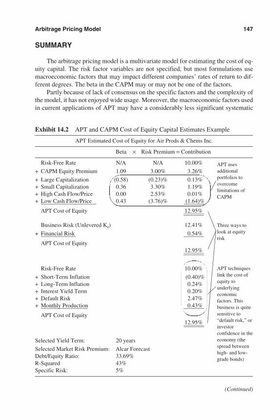
Arbitrage Pricing Model 147
Exhibit 14.2 APT and CAPM Cost of Equity Capital Estimates Example
APT Estimated Cost of Equity for Air Prods & Chems Inc.
Beta × Risk Premium = Contribution
Risk-Free Rate
+ CAPM Equity Premium
+ Large Capitalization+ Small Capitalization+ High Cash Flow/Price+ Low Cash Flow/Price—————————–
APT Cost of Equity
Business Risk (Unlevered Ke) 12.41%
+ Financial Risk 0.54%—————— ———–APT Cost of Equity
12.95%———–———–
Risk-Free Rate 10.00%
+ Short-Term Inflation (0.40)%+ Long-Term Inflation 0.24%+ Interest Yield Term 0.20%+ Default Risk 2.47%+ Monthly Production 0.43%———————–– ———–
APT Cost of Equity12.95%———–———–
Selected Yield Term: 20 years
Selected Market Risk Premium: Alcar ForecastDebt/Equity Ratio: 33.69%R-Squared 43%Specific Risk: 5%
N/A N/A 10.00%
1.09 3.00% 3.26%
(0.58) (0.23)% 0.13%0.36 3.30% 1.19%0.00 2.53% 0.01%0.43 (3.76)% (1.64)%———–
12.95%———–———–
APT usesadditionalportfolios toovercomelimitations ofCAPM
Three ways tolook at equityrisk
APT techniqueslink the cost ofequity tounderlyingeconomicfactors. Thisbusiness is quitesensitive to“default risk,” orinvestorconfidence in theeconomy (thespread betweenhigh- and low-grade bonds)
(Continued)
SUMMARY
The arbitrage pricing model is a multivariate model for estimating the cost of eq-uity capital. The risk factor variables are not specified, but most formulations usemacroeconomic factors that may impact different companies’ rates of return to dif-ferent degrees. The beta in the CAPM may or may not be one of the factors.
Partly because of lack of consensus on the specific factors and the complexity ofthe model, it has not enjoyed wide usage. Moreover, the macroeconomic factors usedin current applications of APT may have a considerably less significant systematic
3953 P-14 8/29/02 2:24 PM Page 147
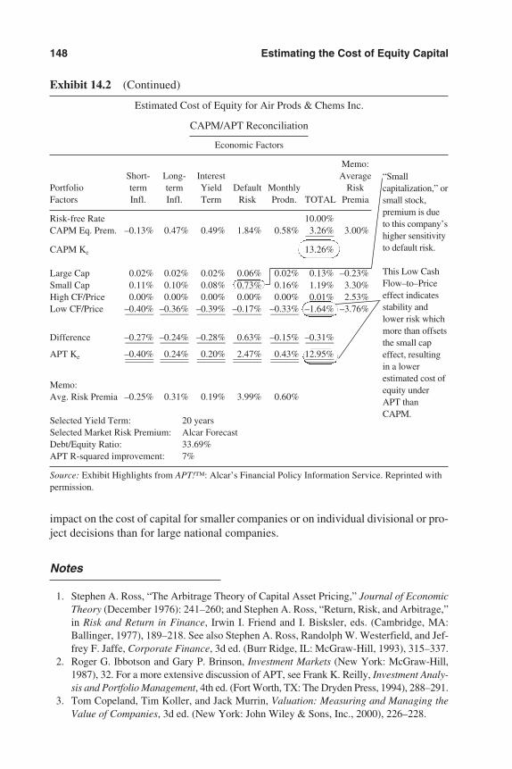
impact on the cost of capital for smaller companies or on individual divisional or pro-ject decisions than for large national companies.
Notes
1. Stephen A. Ross, “The Arbitrage Theory of Capital Asset Pricing,” Journal of EconomicTheory (December 1976): 241–260; and Stephen A. Ross, “Return, Risk, and Arbitrage,”in Risk and Return in Finance, Irwin I. Friend and I. Bisksler, eds. (Cambridge, MA:Ballinger, 1977), 189–218. See also Stephen A. Ross, Randolph W. Westerfield, and Jef-frey F. Jaffe, Corporate Finance, 3d ed. (Burr Ridge, IL: McGraw-Hill, 1993), 315–337.
2. Roger G. Ibbotson and Gary P. Brinson, Investment Markets (New York: McGraw-Hill,1987), 32. For a more extensive discussion of APT, see Frank K. Reilly, Investment Analy-sis and Portfolio Management, 4th ed. (Fort Worth, TX: The Dryden Press, 1994), 288–291.
3. Tom Copeland, Tim Koller, and Jack Murrin, Valuation: Measuring and Managing theValue of Companies, 3d ed. (New York: John Wiley & Sons, Inc., 2000), 226–228.
148 Estimating the Cost of Equity Capital
Exhibit 14.2 (Continued)
Estimated Cost of Equity for Air Prods & Chems Inc.
CAPM/APT Reconciliation
Economic Factors
Memo:Short- Long- Interest Average
Portfolio term term Yield Default Monthly RiskFactors Infl. Infl. Term Risk Prodn. TOTAL Premia
Risk-free Rate 10.00%CAPM Eq. Prem. –0.13% 0.47% 0.49% 1.84% 0.58% 3.26% 3.00%———
CAPM Ke 13.26%
Large Cap 0.02% 0.02% 0.02% 0.06% 0.02% 0.13% –0.23%Small Cap 0.11% 0.10% 0.08% 0.73% 0.16% 1.19% 3.30%High CF/Price 0.00% 0.00% 0.00% 0.00% 0.00% 0.01% 2.53%Low CF/Price –0.40% –0.36% –0.39% –0.17% –0.33% –1.64% –3.76%——— ——— ——— ——— ——— ———
Difference –0.27% –0.24% –0.28% 0.63% –0.15% –0.31%——— ——— ——— ——— ——— ———APT Ke –0.40% 0.24% 0.20% 2.47% 0.43% 12.95%——— ——— ——— ——— ——— —————— ——— ——— ——— ——— ———
Memo:Avg. Risk Premia –0.25% 0.31% 0.19% 3.99% 0.60%
Selected Yield Term: 20 yearsSelected Market Risk Premium: Alcar ForecastDebt/Equity Ratio: 33.69%APT R-squared improvement: 7%
Source: Exhibit Highlights from APT!™: Alcar’s Financial Policy Information Service. Reprinted withpermission.
“Smallcapitalization,” orsmall stock,premium is dueto this company’shigher sensitivityto default risk.
This Low CashFlow–to–Priceeffect indicatesstability andlower risk whichmore than offsetsthe small capeffect, resultingin a lowerestimated cost ofequity underAPT thanCAPM.
3953 P-14 8/29/02 2:24 PM Page 148
PART III
Other Topics Relatedto Cost of Capital
3953 P-15 8/29/02 2:25 PM Page 149

3953 P-15 8/29/02 2:25 PM Page 150
151
Chapter 15
Minority versus ControlImplications of Cost ofCapital DataMinority versus Control Has Little or No Impact on Cost of CapitalCompany Efficiency versus Shareholder ExploitationImpact of the Standard of ValueUnder What Circumstances Should a Control Premium Be Applied?
Projected Income May Not Reflect What a Control Owner Would AchieveInvestment Value Reflecting SynergiesFactors Affecting a Control Premium a Financial Buyer Might Pay
A Tale of Two MarketsMany Takeovers at Less Than Public Trading PriceSummary
There is much confusion about whether the results of applying cost of capital data,as discussed in this book, in the context of a company or stock valuation produces aminority value or a control value. The difference between the per-share value of ashare that represents control and the per-share value of a share that represents a mi-nority interest can be quite significant. (See, e.g., the traditional “levels of value” chart,Exhibit 15.1.) As with many such questions in economics and finance, the answer is:It depends.
More than anything else, when the cost of capital is used in the context of valu-ation, the question of whether the result of discounting or capitalizing represents aminority or a control value depends primarily on the nature of the cash flows beingdiscounted or capitalized rather than on the discount or capitalization rate.
In some cases, the answer to this question may hinge on the definition of valuesought, for example, fair market value (the value to a hypothetical buyer and/or seller)or investment value (the value to a particular buyer and/or seller).1
3953 P-15 8/29/02 2:25 PM Page 151
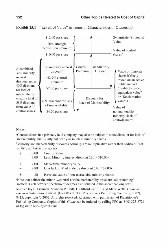
152 Other Topics Related to Cost of Capital
Exhibit 15.1 “Levels of Value” in Terms of Characteristics of Ownership
Notes:aControl shares in a privately held company may also be subject to some discount for lack ofmarketability, but usually not nearly as much as minority shares.
bMinority and marketability discounts normally are multiplicative rather than additive. Thatis, they are taken in sequence:
$ 10.00 Control Value– 3.00 Less: Minority interest discount (.30 × $10.00)—————–$ 7.00 Marketable minority value– 2.80 Less lack of Marketability discount (.40 × $7.00)—————–$ 4.20 Per share value of non-marketable minority shares
cNote that neither the minority/control nor the marketability issue are “all or nothing”matters. Each covers a spectrum of degrees as discussed in the accompanying text.
Source: Jay E. Fishman, Shannon P. Pratt, J. Clifford Griffith, and Mark Wells, Guide toBusiness Valuations, 12th ed. (Fort Worth, TX: Practitioners Publishing Company, 2002),8–15, copyright © 2002. All rights reserved. Reprinted with permission of Practitioner’sPublishing Company. Copies of this Guide can be ordered by calling PPC at (800) 323-8724or log on to www.ppcnet.com.
A combined30% minorityinterestdiscount and a40% discountfor lack ofmarketabilityequals a total of58% discountfrom value ofcontrol sharesb
$12.00 per share
20% strategicacquisition premium
$10.00 per share
30% minority interestdiscountc
42.9% controlpremium
$7.00 per share
40% discount for lackof marketabilityc
$4.20 per share
Synergistic (Strategic)Value
Value of controlsharesa
Value of minorityshares if freelytraded on an activepublic market(“Publicly tradedequivalent value”or “Stock marketvalue”)
Value ofnonmarketableminority (lack ofcontrol) shares
Control or MinorityPremium Discount
Discount for Lack of Marketability
{
{{ {{
3953 P-15 8/29/02 2:25 PM Page 152
MINORITY VERSUS CONTROL HAS LITTLE OR NO IMPACT ONCOST OF CAPITAL
Regardless of which of the major approaches is used to estimate cost of capital(e.g., build-up model, Capital Asset Pricing Model, discounted cash flow model, orarbitrage pricing model), the information is derived from publicly traded stocks. Be-cause these public market transactions represent minority ownership interests, someanalysts think that the cost of capital should be adjusted downward in valuing a con-trolling ownership interest.
This generally is not true!Recall that the discounting method of valuation and the capitalization method of
valuation have two basic elements in common:
1. A numerator consisting of an amount or amounts of expected economic income
2. A denominator consisting of a rate of return at which the economic income isdiscounted or capitalized
Almost all the difference in the control value versus the minority value in the incomeapproach to valuation is found in the numerator—the expected economic incomeavailable to the investor—rather than in the denominator—the discount or capital-ization rate.
As Roger Ibbotson has succinctly stated the case:
When you are purchasing a company you are acquiring the ability to potentially controlfuture cash flows. To acquire this option to exercise control, you must pay a premium.Holding all else constant, it should not impact the discount rate.2
Generally speaking, investors will not accept a lower expected rate of return forpurchase of a controlling interest than for purchase of a minority interest. Controlbuyers pay premiums because they expect to do something to increase the cash flows,not because they are willing to accept a lower expected rate of return. What they maydo to increase cash flows can range from eliminating inactive relatives from the pay-roll to drastically increasing prices for products or services of both acquirer and tar-get as a result of absorbing a direct competitor.
Of course, many a public stock has taken a huge tumble in its market price as aresult of an acquisition. This usually is because the acquisition failed to achieve theexpected increase in cash flows for the target and/or the acquirer. If the market per-ceives that the returns a company is likely to achieve will fall short of the market’srequired rate of return, then the market simply adjusts the stock price downwarduntil the expected returns do meet the market’s required rate of return.
The “control premium” in Mergerstat/Shannon Pratt’s Control Premium Study™includes both the “control premium” and the “synergistic” or “strategic” premium, asshown in Exhibit 15.1.
Minority versus Control Implications of Cost of Capital Data 153
3953 P-15 8/29/02 2:25 PM Page 153
COMPANY EFFICIENCY VERSUS SHAREHOLDEREXPLOITATION
Benefits available to a minority shareholder are a function of two distinct factors:
1. Efficiency at the overall company level
2. Differential benefits between control stockholders and minority stockholders(e.g., cash flow that could be available for dividends used for extra compensationto controlling owners)
Controlling stockholders enjoy a number of prerogatives of control, which canhave an impact on both of the aforementioned factors as they affect minority stock-holders. Some of the more common prerogatives of control include the ability to:
• Appoint or change operational management.
• Appoint or change members of the board of directors.
• Determine management compensation and perquisites.
• Set operational and strategic policy and change the course of the business.
• Acquire, lease, or liquidate business assets, including plant, property, andequipment.
• Select suppliers, vendors, and subcontractors with whom to do business and awardcontracts.
• Negotiate and consummate mergers and acquisitions.
• Liquidate, dissolve, sell out, or recapitalize the company.
• Sell or acquire Treasury shares.
• Register the company’s equity securities for an initial or secondary public offering.
• Register the company’s debt securities for an initial or secondary public offering.
• Declare and pay cash and/or stock dividends.
• Change the articles of incorporation or bylaws.
• Set one’s own compensation (and perquisites) and the compensation (andperquisites) of related-party employees.
• Select joint venturers and enter into joint venture and partnership agreements.
• Decide what products and/or services to offer and how to price those products/services.
• Decide what markets and locations to serve, to enter into, and to discontinueserving.
• Decide which customer categories to market to and which not to market to.
• Enter into inbound and outbound license or sharing agreements regarding intel-lectual properties.
• Block any or all of the above actions.3
154 Other Topics Related to Cost of Capital
3953 P-15 8/29/02 2:25 PM Page 154
It is apparent that exercise of some of these prerogatives may have an impact onthe total cash flows available to the firm, and others will affect the relative benefitsultimately realized by control shareholders versus minority shareholders. It shouldalso be apparent that in projecting expected cash flows, the amounts available to a con-trol owner may not be the same as those available to a minority owner. For example,in many companies control owners set their own compensation (often reflecting theirown perceived genius) rather than having an independent compensation committee. Inany case, whether a result of company efficiency or differential shareholder benefits,it is the expected cash flows to the investor that drive the value to the investor, not dif-ferences in cost of capital between minority investors and control investors.
Enron and its ilk notwithstanding, the exploitation of minority shareholders is farless prevalent in public companies than in private companies, at least in larger pub-lic companies. If company cash flows are already maximized and the returns are al-ready distributed pro rata to all shareholders, then there may be no difference betweena control value and a minority value.
IMPACT OF THE STANDARD OF VALUE
Some analysts suggest that the appropriate cost of capital for an acquisitionshould be that of the acquirer rather than the target. This position departs from the stan-dard of fair market value (the price at which the property would change hands betweenhypothetical buyers and sellers, with no special motivations) and introduces an ele-ment of investment value (the value to a particular buyer or seller). If the standard ofvalue is fair market value, then the principle that “The cost of capital is a function ofthe investment, not the investor” clearly applies.
The idea of fair market value is that there is a consensus value that, in economicterms, “clears the market.” If the cost of capital is a function of the investment, notthe investor, then it is conceivable that the risk perceived by one investor may departfrom the market consensus regarding the investment’s risk. If the estimated cost ofcapital for a particular investment for a particular investor is driven by a view that de-parts from the market consensus, then we are moving away from the standard of fairmarket value (a consensus value) and toward investment value (value to some par-ticular investor, driven by that investor’s unique perceptions or circumstances).
UNDER WHAT CIRCUMSTANCES SHOULD A CONTROLPREMIUM BE APPLIED?
We have made the case that the cost of capital is the same or nearly the same forcontrolling interests as for minority interests. But we know that acquisitions are madeat prices reflecting a control price premium over public market minority share trad-ing prices.4 So if we are valuing a controlling interest by the discounting or capital-izing method, and if we are using the cost of capital that we have estimated, under whatcircumstances should we add a control premium?
Minority versus Control Implications of Cost of Capital Data 155
3953 P-15 8/29/02 2:25 PM Page 155
Projected Income May Not Reflect What a Control Owner Would Achieve
We said earlier that the control premium would be reflected as a result of the in-creased cash flows that a control owner would expect to achieve. If such control cashflows have been either discounted or capitalized, then little or no further control pre-mium should be applied. However, if the projected cash flows used do not reflect acontrol owner’s expectations, then a control premium may be warranted.
Investment Value Reflecting Synergies
If a buyer may achieve strategic or synergistic benefits by an acquisition, thenthat buyer may be willing to pay a control premium. For example, if the target is a di-rect competitor, then the buyer may benefit by raising his or her own prices as wellas those of the target. Remember, however, that a price premium reflecting benefitsto such a particular buyer brings in the element of investment value as opposed to apure fair market value.
In the context of this thinking, the “levels of value” chart (Exhibit 15.1) addedanother level at the top since the first edition of this book was published, “synergis-tic value,” reflecting a potential premium over control value on a stand-alone basis.
Factors Affecting a Control Premium a Financial Buyer Might Pay
Financial buyers sometimes pay control premiums, even if they do not have anyopportunities for synergistic benefits, albeit typically much lower premiums than thosepaid by synergistic buyers. For example, one control prerogative that control ownerscan implement that minority owners cannot is to register a public offering. Other con-trol prerogatives would be to sell interests to employees or to others, to repurchase out-standing minority interests, or to recapitalize. Some will pay a premium to “call theshots.” Some may perceive psychological advantages to control of certain companies.
A TALE OF TWO MARKETS
In my opinion, a strong case could be made that when the share price of a publiccompany is wildly out of line with its intrinsic value (to a financial buyer, and even pos-sibly to a normal strategic buyer), then perhaps the public market value is meaninglessand should be disregarded entirely.
In 2001 Mark Lee, a well-known business valuation analyst for over 25 years,went public with his views on the issue. Lee observed:
The stock market is a market for minority interests in common stock. The principal buy-ers and sellers are individuals, mutual funds, and financial institutions. The market ishighly liquid, individual investment horizons may be short, and risk tolerances can be
156 Other Topics Related to Cost of Capital
3953 P-15 8/29/02 2:25 PM Page 156
greater than in illiquid markets. Financing is often readily available from banks and bro-kers at short-term money rates. Investors are generally passive. Individual investmentsare usually purchased as part of diversified portfolios, which leads to greater tolerance torisk.
The [mergers and acquisitions] market is a market for whole companies. The prin-cipal buyers and sellers are controlling shareholders, corporations, and [leveraged buy-out] houses. The market is not liquid; as a result, individual investment horizons tend tobe longer. Risk tolerances in the short term tend to be lower than in a liquid market.Transactions are financed using long-term debt from banks, insurance companies, mez-zanine funds, equity of large corporations, and private equity funds. [Mergers and ac-quisitions] investors take an active role in managing their companies.
The relationship of the two markets is not linear [as shown in the single bar of thelevels of value chart]. [This linearity] presupposes that acquisition premiums apply in allsituations; and acquisition premiums are roughly the same amount generally or in eachindustry.
The relationship of the two markets is better shown as the two overlapping forms asshown in [Exhibit 15.2]. . . .
Clearly, the existence of an acquisition premium and its magnitude is a “facts andcircumstances” test for each individual valuation.5
It is obvious that one must be extremely cautious about applying a control pre-mium to public market values to determine a control level of value. Conversely, ifguideline stocks are trading at or near control value in a given case, valuation of a mi-nority interest by applying a discount for lack of control from the guideline indicators(in addition to a lack of marketability discount) might be supported since the minor-ity owner lacks the control prerogative of taking the company public or registeringhis or her stock in an offering.
MANY TAKEOVERS AT LESS THAN PUBLIC TRADING PRICE
Many people are surprised to learn just how many takeovers occur at pricesbelow the public trading price. In 2001, Business Valuation Resources assumed dis-tribution of the Mergerstat Control Premium Study™, renamed it Mergerstat/Shan-non Pratt’s Control Premium Study™, and put it online so that people could accessand analyze it electronically. Utilizing this, Exhibit 15.3 is a summary of thetakeovers of public companies from 1998 through 2001.
In the 16 quarters analyzed, over 16% of the takeovers were at prices below theirrecent public market trading prices! Also as shown in Exhibit 15.3, including the“negative premiums” in the medians and averages has a dramatic impact.
The database is searchable by Standard Industrial Classification (SIC) code,North American Industry Classification System (NAICS) code, time frame, and sizeof company (by several measurements). Before naively applying an “average” con-trol premium or implied minority discount, I would recommend searching the data-base to select those transactions that are truly relevant to the subject at hand.6
Minority versus Control Implications of Cost of Capital Data 157
3953 P-15 8/29/02 2:25 PM Page 157
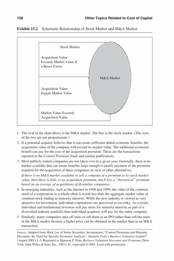
158 Other Topics Related to Cost of Capital
Exhibit 15.2 Schematic Relationship of Stock Market and M&A Market
Stock Market
1. The oval in the chart above is the M&A market. The box is the stock market. (The sizesof the two are not proportionate.)
2. If a potential acquirer believes that it can create sufficient added economic benefits, theacquisition value of the company will exceed its market value. The additional economicbenefit can pay for the cost of the acquisition premium. These are the transactionsreported in the Control Premium Study and similar publications.
3. Most publicly traded companies are not taken over in a given year. Generally, there is nomarket available that can create benefits large enough to justify payment of the premiumrequired for the acquisition of these companies in view of other alternatives.
If there is no M&A market available to sell a company at a premium to its stock marketvalue, then there is little or no acquisition premium, much less a “theoretical” premiumbased on an average of acquisitions of dissimilar companies.
4. In emerging industries, such as the Internet in 1998 and 1999, the value of the commonstock of a corporation as a whole often is worth less than the aggregate market value ofcommon stock trading as minority interests. While the new industry is viewed as veryattractive for investment, individual corporations are perceived as too risky. As a result,individual and institutional investors will pay more for minority interests as part of adiversified industry portfolio than individual acquirers will pay for the entire company.
5. Similarly, many companies spin off units or sell them in an IPO rather than sell the unitsin the M&A market because a higher price can be obtained in the market than in an M&Atransaction.
Source: Adapted from Mark Lee of Sutter Securities, Incorporated, “Control Premiums and MinorityDiscounts: the Need for Specific Economic Analysis.” Shannon Pratt’s Business Valuation Update®
(August 2001):1–5. Reprinted in Shannon P. Pratt, Business Valuation Discounts and Premiums (NewYork: John Wiley & Sons, Inc., 2001), 41, copyright © 2001. Used with permission.
Acquisition ValueExceeds Market Value Ifa Buyer Exists
Acquisition ValueEquals Market Value
Market Value ExceedsAcquisition Value
M&A Market
3953 P-15 8/29/02 2:25 PM Page 158
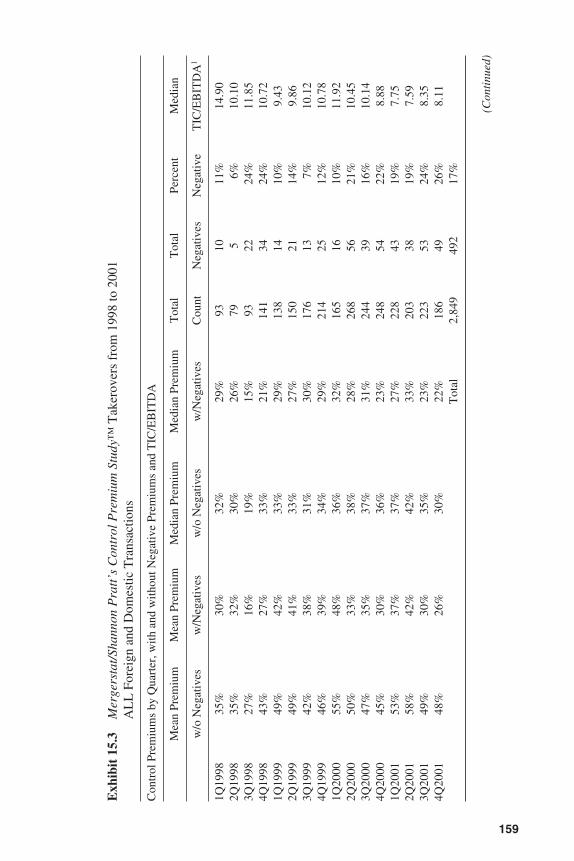
159
Exh
ibit
15.
3M
erge
rsta
t/Sh
anno
n P
ratt
’s C
ontr
ol P
rem
ium
Stu
dy™
Tak
erov
ers
from
199
8 to
200
1A
LL
For
eign
and
Dom
estic
Tra
nsac
tions
Con
trol
Pre
miu
ms
by Q
uart
er, w
ith a
nd w
ithou
t Neg
ativ
e Pr
emiu
ms
and
TIC
/EB
ITD
A
Mea
n Pr
emiu
mM
ean
Prem
ium
Med
ian
Prem
ium
Med
ian
Prem
ium
Tot
alT
otal
Perc
ent
Med
ian
w/o
Neg
ativ
esw
/Neg
ativ
esw
/o N
egat
ives
w/N
egat
ives
Cou
ntN
egat
ives
Neg
ativ
eT
IC/E
BIT
DA
1
1Q19
9835
%30
%32
%29
%93
1011
%14
.90
2Q19
9835
%32
%30
%26
%79
56%
10.1
03Q
1998
27%
16%
19%
15%
9322
24%
11.8
54Q
1998
43%
27%
33%
21%
141
3424
%10
.72
1Q19
9949
%42
%33
%29
%13
814
10%
9.43
2Q19
9949
%41
%33
%27
%15
021
14%
9.86
3Q19
9942
%38
%31
%30
%17
613
7%10
.12
4Q19
9946
%39
%34
%29
%21
425
12%
10.7
81Q
2000
55%
48%
36%
32%
165
1610
%11
.92
2Q20
0050
%33
%38
%28
%26
856
21%
10.4
53Q
2000
47%
35%
37%
31%
244
3916
%10
.14
4Q20
0045
%30
%36
%23
%24
854
22%
8.88
1Q20
0153
%37
%37
%27
%22
843
19%
7.75
2Q20
0158
%42
%42
%33
%20
338
19%
7.59
3Q20
0149
%30
%35
%23
%22
353
24%
8.35
4Q20
0148
%26
%30
%22
%18
649
26%
8.11
Tot
al2,
849
492
17%
(Con
tinu
ed)
3953 P-15 8/29/02 2:25 PM Page 159
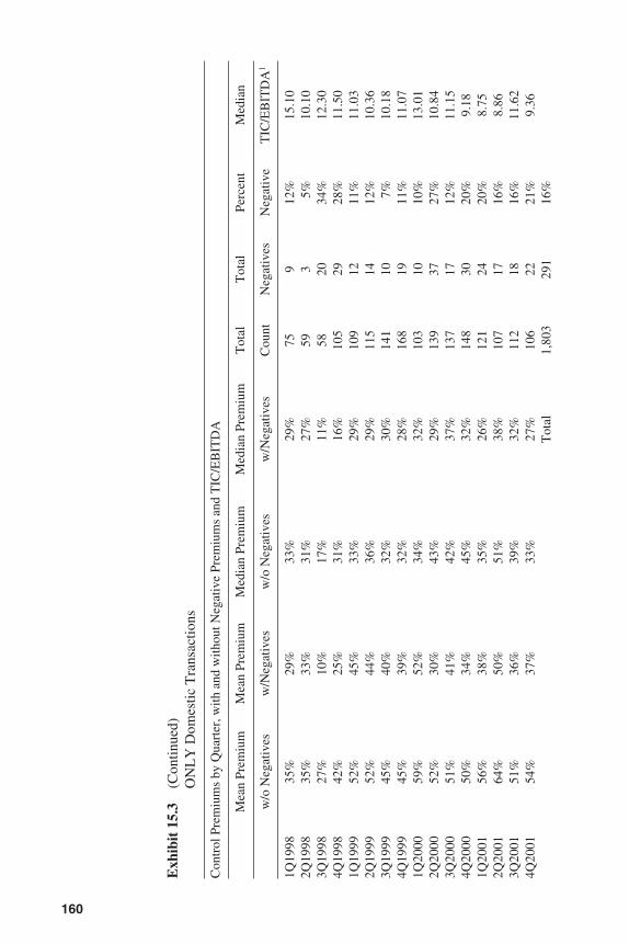
160
Exh
ibit
15.
3(C
ontin
ued)
ON
LY
Dom
estic
Tra
nsac
tions
Con
trol
Pre
miu
ms
by Q
uart
er, w
ith a
nd w
ithou
t Neg
ativ
e Pr
emiu
ms
and
TIC
/EB
ITD
A
Mea
n Pr
emiu
mM
ean
Prem
ium
Med
ian
Prem
ium
Med
ian
Prem
ium
Tot
alT
otal
Perc
ent
Med
ian
w/o
Neg
ativ
esw
/Neg
ativ
esw
/o N
egat
ives
w/N
egat
ives
Cou
ntN
egat
ives
Neg
ativ
eT
IC/E
BIT
DA
1
1Q19
9835
%29
%33
%29
%75
912
%15
.10
2Q19
9835
%33
%31
%27
%59
35%
10.1
03Q
1998
27%
10%
17%
11%
5820
34%
12.3
04Q
1998
42%
25%
31%
16%
105
2928
%11
.50
1Q19
9952
%45
%33
%29
%10
912
11%
11.0
32Q
1999
52%
44%
36%
29%
115
1412
%10
.36
3Q19
9945
%40
%32
%30
%14
110
7%10
.18
4Q19
9945
%39
%32
%28
%16
819
11%
11.0
71Q
2000
59%
52%
34%
32%
103
1010
%13
.01
2Q20
0052
%30
%43
%29
%13
937
27%
10.8
43Q
2000
51%
41%
42%
37%
137
1712
%11
.15
4Q20
0050
%34
%45
%32
%14
830
20%
9.18
1Q20
0156
%38
%35
%26
%12
124
20%
8.75
2Q20
0164
%50
%51
%38
%10
717
16%
8.86
3Q20
0151
%36
%39
%32
%11
218
16%
11.6
24Q
2001
54%
37%
33%
27%
106
2221
%9.
36T
otal
1,80
329
116
%
3953 P-15 8/29/02 2:25 PM Page 160
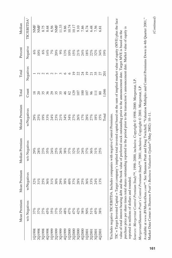
161
Mea
n Pr
emiu
mM
ean
Prem
ium
Med
ian
Prem
ium
Med
ian
Prem
ium
Tot
alT
otal
Perc
ent
Med
ian
w/o
Neg
ativ
esw
/Neg
ativ
esw
/o N
egat
ives
w/N
egat
ives
Cou
ntN
egat
ives
Neg
ativ
eT
IC/E
BIT
DA
1
1Q19
9837
%32
%29
%29
%18
16%
NM
F2Q
1998
37%
31%
28%
25%
202
10%
NM
F3Q
1998
27%
25%
23%
19%
352
6%8.
754Q
1998
45%
36%
35%
33%
365
14%
8.68
1Q19
9935
%31
%24
%24
%29
27%
6.56
2Q19
9937
%30
%25
%23
%35
720
%N
MF
3Q19
9932
%29
%26
%21
%35
39%
11.3
34Q
1999
48%
38%
38%
34%
466
13%
9.86
1Q20
0047
%40
%37
%34
%62
610
%10
.74
2Q20
0047
%37
%32
%27
%12
919
15%
10.1
73Q
2000
42%
28%
32%
26%
107
2221
%9.
104Q
2000
38%
25%
24%
17%
100
2424
%7.
861Q
2001
50%
36%
37%
28%
107
1918
%6.
742Q
2001
51%
33%
36%
27%
9621
22%
6.48
3Q20
0145
%24
%31
%18
%11
135
32%
7.56
4Q20
0138
%13
%25
%15
%80
2734
%6.
81T
otal
1,04
620
119
%
1 Exc
lude
s ne
gativ
e T
IC/E
BIT
DA
. Inc
lude
s co
mpa
nies
with
neg
ativ
e C
ontr
ol P
rem
ium
s.1 T
IC =
Tar
get I
nves
ted
Cap
ital =
Tar
get c
ompa
ny’s
impl
ied
tota
l inv
este
d ca
pita
l bas
ed o
n th
e su
m o
f im
plie
d m
arke
t val
ue o
f eq
uity
(M
VE
) pl
us th
e fa
ceva
lue
of to
tal i
nter
est b
eari
ng d
ebt a
nd th
e bo
ok v
alue
of
pref
erre
d st
ock
outs
tand
ing
prio
r to
the
anno
unce
men
t dat
e. T
arge
t MV
E is
bas
ed o
n th
epu
rcha
se p
rice
per
sha
re ti
mes
tota
l sha
res
outs
tand
ing
repo
rted
in th
e pe
riod
pri
or to
the
tran
sact
ion’
s an
noun
cem
ent d
ate.
Mar
ket v
alue
of
equi
ty is
repo
rted
in m
illio
ns o
f do
llars
and
rou
nded
.
Sour
ces:
Mer
gers
tat C
ontr
ol P
rem
ium
Stu
dy™
, 199
8–20
00, i
nclu
sive
. Cop
yrig
ht ©
1998
–200
0. M
erge
rsta
t, L
P.
Mer
gers
tat/
Shan
non
Pra
tt’s
Con
trol
Pre
miu
m S
tudy
™, 2
001,
incl
usiv
e. C
opyr
ight
©20
01. M
erge
rsta
t, L
P.
Ava
ilabl
e at
ww
w.B
VM
arke
tDat
a.co
msm
. See
Sha
nnon
Pra
tt an
d D
oug
Tw
itche
ll, “
Val
uatio
n M
ultip
les
and
Con
trol
Pre
miu
ms
Dow
n in
4th
Qua
rter
200
1,”
Mar
ket D
ata
Cor
ner
in S
hann
on P
ratt
’s B
usin
ess
Val
uati
on U
pdat
e®(M
ay 2
002)
: 10–
11.
(Con
tinu
ed)
3953 P-15 8/29/02 2:25 PM Page 161
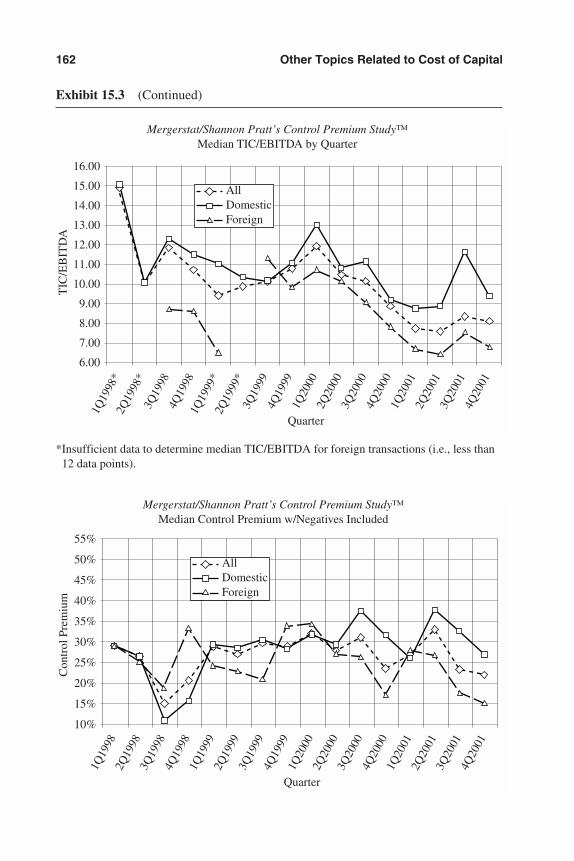
162 Other Topics Related to Cost of Capital
Exhibit 15.3 (Continued)
AllDomesticForeign
Mergerstat/Shannon Pratt’s Control Premium Study™Median TIC/EBITDA by Quarter
16.00
15.00
14.00
13.00
12.00
11.00
10.00
9.00
8.00
7.00
6.00
1Q19
98*
2Q19
98*
3Q19
984Q
1998
1Q19
99*
2Q19
99*
3Q19
994Q
1999
1Q20
002Q
2000
3Q20
004Q
2000
1Q20
012Q
2001
3Q20
014Q
2001
Quarter
TIC
/EB
ITD
A
AllDomesticForeign
Mergerstat/Shannon Pratt’s Control Premium Study™Median Control Premium w/Negatives Included
55%
50%
45%
40%
35%
30%
25%
20%
15%
10%
1Q19
982Q
1998
3Q19
984Q
1998
1Q19
992Q
1999
3Q19
994Q
1999
1Q20
002Q
2000
3Q20
004Q
2000
1Q20
012Q
2001
3Q20
014Q
2001
Quarter
Con
trol
Pre
miu
m
*Insufficient data to determine median TIC/EBITDA for foreign transactions (i.e., less than12 data points).
3953 P-15 8/29/02 2:25 PM Page 162
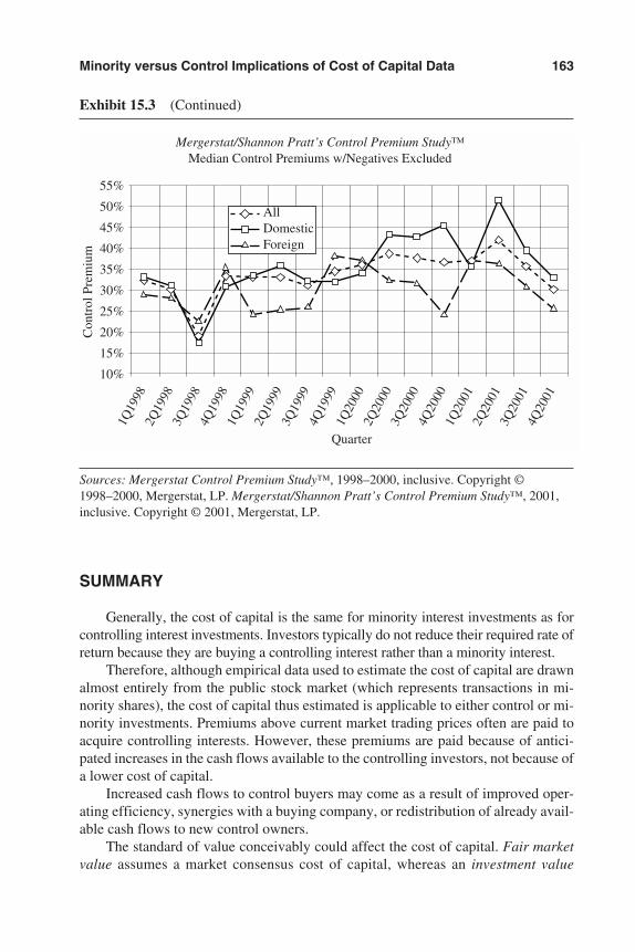
SUMMARY
Generally, the cost of capital is the same for minority interest investments as forcontrolling interest investments. Investors typically do not reduce their required rate ofreturn because they are buying a controlling interest rather than a minority interest.
Therefore, although empirical data used to estimate the cost of capital are drawnalmost entirely from the public stock market (which represents transactions in mi-nority shares), the cost of capital thus estimated is applicable to either control or mi-nority investments. Premiums above current market trading prices often are paid toacquire controlling interests. However, these premiums are paid because of antici-pated increases in the cash flows available to the controlling investors, not because ofa lower cost of capital.
Increased cash flows to control buyers may come as a result of improved oper-ating efficiency, synergies with a buying company, or redistribution of already avail-able cash flows to new control owners.
The standard of value conceivably could affect the cost of capital. Fair marketvalue assumes a market consensus cost of capital, whereas an investment value
Minority versus Control Implications of Cost of Capital Data 163
AllDomesticForeign
Mergerstat/Shannon Pratt’s Control Premium Study™Median Control Premiums w/Negatives Excluded
55%
50%
45%
40%
35%
30%
25%
20%
15%
10%
1Q19
982Q
1998
3Q19
984Q
1998
1Q19
992Q
1999
3Q19
994Q
1999
1Q20
002Q
2000
3Q20
004Q
2000
1Q20
012Q
2001
3Q20
014Q
2001
Quarter
Con
trol
Pre
miu
m
Exhibit 15.3 (Continued)
Sources: Mergerstat Control Premium Study™, 1998–2000, inclusive. Copyright ©1998–2000, Mergerstat, LP. Mergerstat/Shannon Pratt’s Control Premium Study™, 2001,inclusive. Copyright © 2001, Mergerstat, LP.
3953 P-15 8/29/02 2:25 PM Page 163
164 Other Topics Related to Cost of Capital
standard may reflect a cost of capital driven by a particular investor’s perceptions orcircumstances, which may depart from the market consensus.
The merger and acquisition market is a distinct market from the public stock mar-ket. While most takeovers occur at prices above the stock’s public market price prior tothe acquisition, a significant number occur at prices below the public market tradingprice. Careful research should be undertaken before applying a “control premium” or“implied minority discount” to a private company valuation to determine whether sucha premium or discount is warranted.
Notes
1. For a detailed discussion of definitions of various standards of value in commonly en-countered legal contexts, see “Standards of Value” in Shannon P. Pratt, Robert F. Reilly,and Robert P. Schweihs, Valuing a Business: The Analysis and Appraisal of Closely HeldCompanies, 4th ed. (New York: McGraw-Hill, 2000), 28–32.
2. Ibbotson Associates Cost of Capital Workshop (Chicago: Ibbotson Associates, 1998),Chapter 1, p. 12.
3. Pratt, Reilly, and Schweihs, Valuing a Business, 347–348, 365–366 (McGraw-Hill): Usedwith permission.
4. See, for example, Mergerstat/Shannon Pratt’s Control Premium Study™ (Los Angeles:Mergerstat, LP), distributed exclusively by Business Valuation Resources, LLC, Portland,Oregon, available online, updated quarterly, at www.BVMarketData.com sm.
5. Mark Lee, “Control Premiums and Minority Discounts: The Need for Specific EconomicAnalysis,” Shannon Pratt’s Business Valuation Update® (August 2001): 1–5. Used withpermission.
6. See, for example, Daniel L. McConaughy, “Negative Takeover Premia and Stock PriceLevels in Internet Stocks,” Valuation Strategies (March/April 2002): 20–29.
3953 P-15 8/29/02 2:25 PM Page 164
165
Chapter 16
Handling the Discount forLack of MarketabilityDiscrete Percentage Discount for Lack of Marketability
Minority Ownership InterestsControlling Ownership Interests
Building the Discount for Lack of Marketability into the Discount RateVenture Capitalists’ Required Rates of ReturnQuantifying the Marketability Factor in the Discount Rate
Summary
As noted earlier, whether the cost of capital estimation is based partly on histor-ical market data or entirely on current market data, the data represent publicly tradedstock transactions in the highly liquid U.S. public stock markets. Investors in com-panies without an established trading market for their stock place a high premium onliquidity or, conversely, demand a high discount for lack of liquidity, compared withcompanies with an established trading market for their stock.
Having estimated required rates of return from market data for publicly tradedstocks, there are two ways to adjust for the lack of liquidity for closely held stock:
1. After estimating a value as if publicly traded, subtract a percentage discount forlack of marketability.
2. Build the lack of marketability factor into the discount rate by adding some num-ber of percentage points into the discount or capitalization rate, developed fromany of the models discussed in earlier chapters of this book.
DISCRETE PERCENTAGE DISCOUNT FOR LACK OFMARKETABILITY1
The most common way to handle the lack of marketability issue is by a percent-age deduction from the value indicated after discounting or capitalizing expectedcash flows at a rate derived from public market data.
3953 P-16 8/29/02 2:25 PM Page 165
Minority Ownership Interests
Many empirical studies have provided extensive transaction data to help quantifythe amount of such a discount in the case of minority interest transactions. The studiesconsistently show a central tendency for discounts for lack of marketability for minor-ity interests to be 30% to 50% from the value as if they were publicly traded. However,it is noteworthy that there are many transactions above and below this range.
For any given valuation developed by the income approach, it is tempting to sim-ply take the average from the studies and apply that as a discount for lack of mar-ketability. However, with the broad ranges around the measures of central tendency,like the minority discount/control premium issue, it is more accurate (and moreconvincing to a court) to select from the available databases those transactions withcharacteristics closest to the subject company to estimate the discount for lack ofmarketability.
Fortunately, since the first edition of this book, two databases have been put on-line to enable researchers to do this. One is a restricted stock study and the other is apre–initial public offering (IPO) study.
Restricted Stock Studies
A “restricted stock” is a stock of a public company that is identical in all respectsto the stock that trades publicly, except that it is restricted from trading on the publicmarket. It could be, for example, stock issued in an acquisition, stock issued in a fi-nancing, or stock of insiders not registered in a public offering. Such stock is, how-ever, eligible for block transactions with institutional and other qualified investors.
The essence of restricted stock studies is to compare the price at which a restrictedstock transaction takes place with the public market price on the same day. The per-centage difference is a proxy for the discount for lack of marketability.
A summary of the restricted stock studies published to date is shown as Exhibit16.1. The Securities and Exchange Commission (SEC) loosened the restrictions in1990, and the average discount went down from the mid-30s to the mid-20s. In 1997the SEC reduced the required holding period under Rule 144 from two years to oneyear, and the average discount was 13% in the only post-1997 study as of press time.The reduction in discounts for restricted stocks should not be interpreted to indicatea reduction in the discount for lack of marketability for minority interests in closelyheld companies, but merely as a reaction to the loosening of restrictions.
The most detailed study to date is The FMV Restricted Stock Study™ by FMVOpinions, Inc. It covers 243 transactions from 1980 through 1997 (the year the SEC cutthe required holding period from two years to one year), with 53 data items for eachtransaction. A sample transaction report from the FMV study is shown as Exhibit 16.2.It was placed online in 2001 and is fully searchable at www.BVMarketData.comsm.
When an analyst is trying to quantify a discount for lack of marketability for aparticular company, he or she can search the database to find companies with com-parable characteristics to use for guidance. Such characteristics might include com-
166 Other Topics Related to Cost of Capital
3953 P-16 8/29/02 2:25 PM Page 166

pany size (measured by either sales or assets), size of the block (as a percentage of thetotal outstanding), earnings (or deficit), and so on.
Pre–Initial Public Offering Studies
When a company goes public for the first time, it is required by the SEC to dis-close in its prospectus all the transactions in its stock for the previous three years. Acomparison of the prices of those transactions with the initial public offering (IPO)price is the essence of the “pre-IPO studies.”
The percentage below the IPO price at which the transactions took place (ad-justed for changes in company fundamentals) is a proxy for the discount for lack ofmarketability. For a long time, only two such series of studies existed, the Willamette
Handling the Discount for Lack of Marketability 167
Exhibit 16.1 Summary of Restricted Stock Transaction Studies
Time Number of Average TimePeriod Study Transactions Discount Period6
1/66–6/69 SEC Institutional Investor 398 25.8%1 A1/68–12/70 Milton Gelman 89 33.0% A1/68–12/72 Robert Trout 60 33.5% A1/68–12/722 Robert Moroney 148 35.6% A1/69–12/73 Michael Maher 33 35.4% A10/78–6/82 Standard Research Consultants 28 45.0%3 A1/81–12/88 William Silber 69 33.8% A1/79–4/92 FMV Opinions, Inc.7 >100 23.0% B1/80–12/96 Management Planning, Inc. 53 27.1% B1/91–12/95 Bruce Johnson 70 20.0% C1/96–4/97 Columbia Financial Advisors 23 21.0%4 C5/97–12/98 Columbia Financial Advisors 15 13.0%5 D
1The average was 32.6% for OTC companies not required to file reports with the Securitiesand Exchange Commission.
2The exact ending month is not specified.3Median.4Median was 14.0.5Median was 9.0.6A Pre-1900 (before SEC loosened reporting requirements)B Straddles 1990 (some before, some after, but more after 1997)C Post-1990 but pre-1997D Post-1997 (after SEC reduced required holding period under Rule 144 from two years to
one year)7FMV Opinions has updated its study through 1997, and it now includes 243 transactionsand is available online at www.BVMarketData.com.
Source: Adapted from Shannon P. Pratt, Business Valuation Discounts and Premiums (NewYork: John Wiley & Sons, Inc., 2001), 81, copyright © 2001. Used with permission.
3953 P-16 8/29/02 2:25 PM Page 167
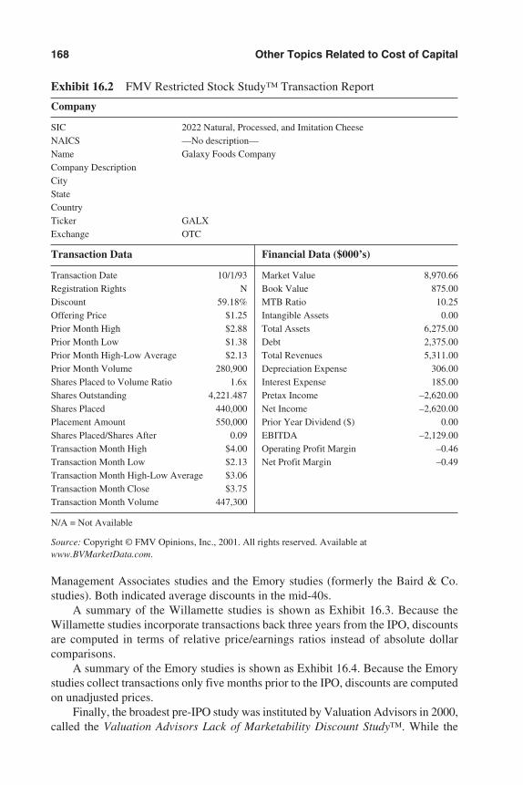
Management Associates studies and the Emory studies (formerly the Baird & Co.studies). Both indicated average discounts in the mid-40s.
A summary of the Willamette studies is shown as Exhibit 16.3. Because theWillamette studies incorporate transactions back three years from the IPO, discountsare computed in terms of relative price/earnings ratios instead of absolute dollarcomparisons.
A summary of the Emory studies is shown as Exhibit 16.4. Because the Emorystudies collect transactions only five months prior to the IPO, discounts are computedon unadjusted prices.
Finally, the broadest pre-IPO study was instituted by Valuation Advisors in 2000,called the Valuation Advisors Lack of Marketability Discount Study™. While the
168 Other Topics Related to Cost of Capital
Exhibit 16.2 FMV Restricted Stock Study™ Transaction Report
Company
SIC 2022 Natural, Processed, and Imitation CheeseNAICS —No description—Name Galaxy Foods CompanyCompany DescriptionCityStateCountryTicker GALXExchange OTC
Transaction Data Financial Data ($000’s)
Transaction Date 10/1/93 Market Value 8,970.66Registration Rights N Book Value 875.00Discount 59.18% MTB Ratio 10.25Offering Price $1.25 Intangible Assets 0.00Prior Month High $2.88 Total Assets 6,275.00Prior Month Low $1.38 Debt 2,375.00Prior Month High-Low Average $2.13 Total Revenues 5,311.00Prior Month Volume 280,900 Depreciation Expense 306.00Shares Placed to Volume Ratio 1.6x Interest Expense 185.00Shares Outstanding 4,221.487 Pretax Income –2,620.00Shares Placed 440,000 Net Income –2,620.00Placement Amount 550,000 Prior Year Dividend ($) 0.00Shares Placed/Shares After 0.09 EBITDA –2,129.00Transaction Month High $4.00 Operating Profit Margin –0.46Transaction Month Low $2.13 Net Profit Margin –0.49Transaction Month High-Low Average $3.06Transaction Month Close $3.75Transaction Month Volume 447,300
N/A = Not Available
Source: Copyright © FMV Opinions, Inc., 2001. All rights reserved. Available atwww.BVMarketData.com.
3953 P-16 8/29/02 2:25 PM Page 168
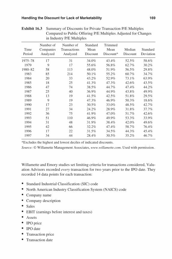
Handling the Discount for Lack of Marketability 169
Exhibit 16.3 Summary of Discounts for Private Transaction P/E MultiplesCompared to Public Offering P/E Multiples Adjusted for Changesin Industry P/E Multiples
Number of Number of Standard TrimmedTime Companies Transactions Mean Mean Median Standard
Period Analyzed Analyzed Discount Discount* Discount Deviation
1975–78 17 31 34.0% 43.4% 52.5% 58.6%1979 9 17 55.6% 56.8% 62.7% 30.2%
1980–82 58 113 48.0% 51.9% 56.5% 29.8%1983 85 214 50.1% 55.2% 60.7% 34.7%1984 20 33 43.2% 52.9% 73.1% 63.9%1985 18 25 41.3% 47.3% 42.6% 43.5%1986 47 74 38.5% 44.7% 47.4% 44.2%1987 25 40 36.9% 44.9% 43.8% 49.9%1988 13 19 41.5% 42.5% 51.8% 29.5%1989 9 19 47.3% 46.9% 50.3% 18.6%1990 17 23 30.5% 33.0% 48.5% 42.7%1991 27 34 24.2% 28.9% 31.8% 37.7%1992 36 75 41.9% 47.0% 51.7% 42.6%1993 51 110 46.9% 49.9% 53.3% 33.9%1994 31 48 31.9% 38.4% 42.0% 49.6%1995 42 66 32.2% 47.4% 58.7% 76.4%1996 17 22 31.5% 34.5% 44.3% 45.4%1997 34 44 28.4% 30.5% 35.2% 46.7%
*Excludes the highest and lowest deciles of indicated discounts.
Source: © Willamette Management Associates, www.willamette.com. Used with permission.
Willamette and Emory studies set limiting criteria for transactions considered, Valu-ation Advisors recorded every transaction for two years prior to the IPO date. Theyrecorded 14 data points for each transaction:
• Standard Industrial Classification (SIC) code
• North American Industry Classification System (NAICS) code
• Company name
• Company description
• Sales
• EBIT (earnings before interest and taxes)
• Assets
• IPO price
• IPO date
• Transaction price
• Transaction date
3953 P-16 8/29/02 2:25 PM Page 169
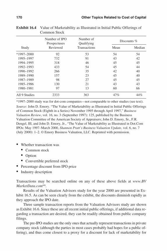
• Whether transaction was
• Common stock
• Option
• Convertible preferred stock
• Percentage discount from IPO price
• Industry description
Transactions may be searched online on any of these above fields at www.BVMarketData.comsm.
Results of the Valuation Advisors study for the year 2000 are presented in Ex-hibit 16.5. As can be seen clearly from the exhibit, the discounts diminish rapidly asthey approach the IPO date.
Three sample transaction reports from the Valuation Advisors study are shownas Exhibit 16.6. Since these are all recent initial public offerings, if additional data re-garding a transaction are desired, they can be readily obtained from public companyfilings.
The pre-IPO studies are the only ones that actually represent transactions in privatecompany stock (although the parties in most cases probably had hopes for a public of-fering), and thus come closest to a proxy for a discount for lack of marketability for
170 Other Topics Related to Cost of Capital
Exhibit 16.4 Value of Marketability as Illustrated in Initial Public Offerings ofCommon Stock
Number of IPO Number ofProspectuses Qualifying
Discounts %
Study Reviewed Transactions Mean Median
*1997–2000 92 53 54 541995–1997 732 91 43 421994–1995 318 46 45 451992–1993 433 54 45 441990–1992 266 35 42 401989–1990 157 23 45 401987–1989 98 27 45 451985–1986 130 21 43 431980–1981 97 13 60 66
All 9 Studies 2333 363 47% 44%
*1997–2000 study was for dot-com companies—not comparable to other studies (see text).
Source: John D. Emory. “The Value of Marketability as Illustrated in Initial Public Offeringsof Common Stock (Eighth in a Series) November 1995 through April 1997,” BusinessValuation Review, vol. 16, no. 3 (September 1997): 125, published by the BusinessValuation Committee of the American Society of Appraisers; John D. Emory, Sr., F.R.Dengel, III, and John D. Emory, Jr., “The Value of Marketability as Illustrated in Dot.ComIPOs: May 1997–March 2000, Shannon Pratt’s Business Valuation Update, vol. 6, no. 7(July 2000): 1–2. © Emory Business Valuation, LLC. Reprinted with permission.
3953 P-16 8/29/02 2:25 PM Page 170
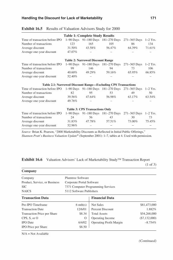
Handling the Discount for Lack of Marketability 171
Exhibit 16.5 Results of Valuation Advisors Study for 2000
Table 1: Complete Study ResultsTime of transaction before IPO 1–90 Days 91–180 Days 181–270 Days 271–365 Days 1–2 Yrs.Number of transactions 123 165 105 86 134Average discount 31.50% 43.58% 56.47% 64.39% 71.61%Average one-year discount 47.07% – – – –
Table 2: Narrowed Discount RangeTime of transaction before IPO 1–90 Days 91–180 Days 181–270 Days 271–365 Days 1–2 Yrs.Number of transactions 99 146 94 73 106Average discount 40.60% 49.29% 59.16% 65.95% 66.85%Average one-year discount 52.40% – – – –
Table 2.1: Narrowed Discount Range—Excluding CPS TransactionsTime of transaction before IPO 1–90 Days 91–180 Days 181–270 Days 271–365 Days 1–2 Yrs.Number of transactions 82 95 53 49 50Average discount 39.56% 47.64% 56.98% 63.17% 63.54%Average one-year discount 49.76% – – – –
Table 3: CPS Transactions OnlyTime of transaction before IPO 1–90 Days 91–180 Days 181–270 Days 271–365 Days 1–2 Yrs.Number of transactions 24 56 43 30 73Average discount 31.83% 47.78% 57.51% 73.00% 75.45%Average one-year discount 52.96% – – – –
Source: Brian K. Pearson, “2000 Marketability Discounts as Reflected in Initial Public Offerings,”Shannon Pratt’s Business Valuation Update® (September 2001): 1–7, tables at 4. Used with permission.
Exhibit 16.6 Valuation Advisors’ Lack of Marketability Study™ Transaction Report (1 of 3)
Company
Company Plumtree SoftwareProduct, Service, or Business Corporate Portal SoftwareSIC 7371 Computer Programming ServicesNAICS 5112 Software Publishers
Transaction Data Financial Data
Pre-IPO Timeframe 6 mth(s) Net Sales $81,473,000Transaction Date 12/6/01 Percent Discount 1.882%Transaction Price per Share $8.34 Total Assets $54,268,000CPS, S, or O O Operating Income ($7,132,000)IPO Date 6/4/02 Operating Profit Margin –8.754%IPO Price per Share $8.50
N/A = Not Available
(Continued)
3953 P-16 8/29/02 2:25 PM Page 171
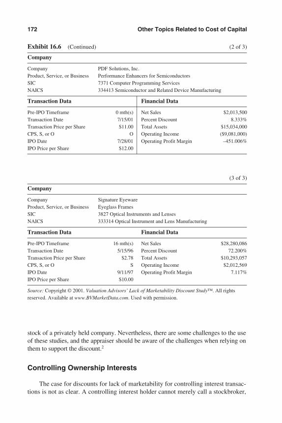
172 Other Topics Related to Cost of Capital
Exhibit 16.6 (Continued) (2 of 3)
Company
Company PDF Solutions, Inc.Product, Service, or Business Performance Enhancers for SemiconductorsSIC 7371 Computer Programming ServicesNAICS 334413 Semiconductor and Related Device Manufacturing
Transaction Data Financial Data
Pre-IPO Timeframe 0 mth(s) Net Sales $2,013,500Transaction Date 7/15/01 Percent Discount 8.333%Transaction Price per Share $11.00 Total Assets $15,034,000CPS, S, or O O Operating Income ($9,081,000)IPO Date 7/28/01 Operating Profit Margin –451.006%IPO Price per Share $12.00
stock of a privately held company. Nevertheless, there are some challenges to the useof these studies, and the appraiser should be aware of the challenges when relying onthem to support the discount.2
Controlling Ownership Interests
The case for discounts for lack of marketability for controlling interest transac-tions is not as clear. A controlling interest holder cannot merely call a stockbroker,
(3 of 3)
Company
Company Signature EyewareProduct, Service, or Business Eyeglass FramesSIC 3827 Optical Instruments and LensesNAICS 333314 Optical Instrument and Lens Manufacturing
Transaction Data Financial Data
Pre-IPO Timeframe 16 mth(s) Net Sales $28,280,086Transaction Date 5/15/96 Percent Discount 72.200%Transaction Price per Share $2.78 Total Assets $10,293,057CPS, S, or O S Operating Income $2,012,569IPO Date 9/11/97 Operating Profit Margin 7.117%IPO Price per Share $10.00
Source: Copyright © 2001. Valuation Advisors’ Lack of Marketability Discount Study™. All rightsreserved. Available at www.BVMarketData.com. Used with permission.
3953 P-16 8/29/02 2:25 PM Page 172
execute a transaction in seconds, and have cash in hand within three business days. Itmay take months to prepare a controlling interest for sale, incurring significant legal,accounting, and management time costs in the process. Furthermore, compared withpublic companies, most private companies have much less ready access to the capi-tal markets to raise additional equity and/or debt capital.
Despite these limitations, some analysts would say that discounts for lack of mar-ketability are not applicable to controlling interests. These same analysts may, however,recognize the realities of these factors under the rubric of “liquidity.” Courts frequentlyhave recognized discounts for lack of marketability for controlling stock interests heldin estates. Discounts for lack of liquidity (marketability) for controlling ownership in-terests, when appropriate (such as those recognized in the U.S. Tax Court), are often inthe range of 10% to 25%,3 not as great as for minority ownership interests.
BUILDING THE DISCOUNT FOR LACK OF MARKETABILITYINTO THE DISCOUNT RATE
Venture Capitalists’ Required Rates of Return
Venture capitalists typically say that they look for expected rates of return be-tween 30% and 50% on their portfolios, which means higher rates on very risky start-ups. One reason why these rates are so high is the illiquidity of the companies andsecurities in which venture capitalists invest, even though they virtually always havean exit strategy in place if everything works out as projected. Unfortunately, there areno data available to indicate how much of their required rate of return is for illiquid-ity. (If any reader can shed light on this issue, please contact the author at the phonenumber or address shown in the preface.)
Quantifying the Marketability Factor in the Discount Rate
In building the lack of marketability factor into the discount rate, determininghow many percentage points to add to the discount rate is difficult and quite subjec-tive. Z. Christopher Mercer, chief executive officer of Mercer Capital, has compileda list of factors to consider, generally adding somewhere between zero and four per-centage points for each factor considered important in the particular case. This list isshown in Exhibit 16.7. In most of his examples, Mercer considers about four to sixfactors, and his cumulative adjustments tend to run between one and six percentagepoints.4 The applicable cash flow for Mercer’s “Quantitative Marketability DiscountModel” discount rate are those expected to be available to the minority investor.
Of course, no empirical basis exists for assigning numbers in a matrix like this,and doing so may give the valuation report a sense of spurious accuracy. When usinga table like this, the analyst might want to include a disclaimer to the effect that thenumbers are presented not for precise quantification, but merely to show the thinkingof the analyst.
Handling the Discount for Lack of Marketability 173
3953 P-16 8/29/02 2:25 PM Page 173
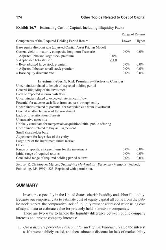
SUMMARY
Investors, especially in the United States, cherish liquidity and abhor illiquidity.Because our empirical data to estimate cost of equity capital all come from the pub-lic stock market, the comparative lack of liquidity must be addressed when using costof capital data to estimate value for privately held interests or companies.
There are two ways to handle the liquidity difference between public companyinterests and private company interests:
1. Use a discrete percentage discount for lack of marketability. Value the interestas if it were publicly traded, and then subtract a discount for lack of marketability
174 Other Topics Related to Cost of Capital
Exhibit 16.7 Estimating Cost of Capital, Including Illiquidity Factor
Range of Returns
Components of the Required Holding Period Return Lower Higher
Base equity discount rate (adjusted Capital Asset Pricing Model)Current yield-to-maturity composite long-term Treasuries 0.0% 0.0%+ Adjusted Ibbotson large stock premium 0.0%× Applicable beta statistic × 1.0= Beta-adjusted large stock premium 0.0% 0.0%+ Adjusted Ibbotson small stock premium 0.0% 0.0%= Base equity discount rate 0.0% 0.0%
Investment-Specific Risk Premiums—Factors to ConsiderUncertainties related to length of expected holding periodGeneral illiquidity of the investmentLack of expected interim cash flowUncertainties related to expected interim cash flowPotential for adverse cash flow from tax pass-through entityUncertainties related to potential for favorable exit from investmentGeneral unattractiveness of the investmentLack of diversification of assetsUnattractive asset mixUnlikely candidate for merger/sale/acquisition/initial public offeringUncertainties related to buy-sell agreementSmall shareholder baseAdjustment for large size of the entityLarge size of the investment limits marketOtherRange of specific risk premiums for the investment 0.0% 0.0%Initial range of required returns 0.0% 0.0%Concluded range of required holding period returns 0.0% 0.0%
Source: Z. Christopher Mercer, Quantifying Marketability Discounts (Memphis: PeabodyPublishing, LP, 1997), 323. Reprinted with permission.
3953 P-16 8/29/02 2:25 PM Page 174
from the estimated publicly traded equivalent value. Two sets of studies to pro-vide quantitative guidance for this are:
1. Restricted stock studies
2. Pre–initial public offering (IPO) studies
2. Adjust the discount rate. Add percentage points to the discount rate used to dis-count the expected cash flows to present value.
The notes provide reference sources for assistance in implementing either one ofthese methods.
Notes
1. For a comprehensive discussion of discounts for lack of marketability, see Chapters 3through 11 in Shannon P. Pratt, Business Valuation Discounts and Premiums (New York:John Wiley & Sons, Inc., 2001), 45–211; see also Chapter 17, “Discounts for Illiquidityand Lack of Marketability,” in Shannon P. Pratt, Robert F. Reilly, and Robert P. Schweihs,Valuing a Business: The Analysis and Appraisal of Closely Held Companies, 4th ed.(New York: McGraw-Hill, 2000), 391–423.
2. See, for example, Shannon Pratt, “Lack of Marketability Discounts Suffer More Contro-versial Attacks,” editor’s column in Shannon Pratt’s Business Valuation Update® (Febru-ary 2002): 1–3; see also Mukesh Bajaj, “Dr. Bajaj Responds to Dr. Pratt’s February 2002Editorial,” reader/editor exchange in Shannon Pratt’s Business Valuation Update® (March2002): 12–14.
3. See reference in note 1; see also Bradley A. Fowler, “How Do You Handle It?” part of aspecial report, “ASA Conference Offers Valuable Insights,” Shannon Pratt’s BusinessValuation Update® (July 1997): 1–2.
4. Z. Christopher Mercer, Quantifying Marketability Discounts: Developing and SupportingMarketability Discounts in the Appraisal of Closely Held Business Interests (Memphis:Peabody Publishing, LP, 1997). This book also comprehensively covers empirical studiesof discounts for lack of marketability conducted over the 30 years up until its publication.
Handling the Discount for Lack of Marketability 175
3953 P-16 8/29/02 2:25 PM Page 175
176
Chapter 17
How Cost of Capital Relatesto the Excess EarningsMethod of ValuationBasic “Excess Earnings” Valuation Method
Conceptual Basis for the MethodSteps in Applying the Excess Earnings MethodExample of the Excess Earnings Method
Cost of Capital Reasonableness CheckComputing the Weighted Average Excess Earnings Capitalization RateEstimating a Build-up Model Capitalization RateDiscussion of the Example
Vagaries of the Excess Earnings MethodSummary
The excess earnings method of valuation was originally created for the purposeof valuing intangible assets, specifically intangible value in the nature of goodwill. Itwas devised to determine how much the U.S. government would compensate brew-ers and distillers for the economic loss of their goodwill as a result of Prohibition.
This valuation method has since been embodied in Revenue Ruling 68-609, in-cluded here as Exhibit 17.1. Although it was originally designed to value only intan-gible assets, it is widely used (and misused) today in the valuation of small businessesand professional practices.
This chapter has a single point: An estimate of the cost of capital, developed bymethods discussed in this book, can be used as a test of the reasonableness of the as-sumptions and results achieved by using the excess earnings method. This test can beapplied either by a person preparing an excess earnings method valuation or by some-one reviewing an excess earnings method valuation prepared by someone else.
This chapter gives only enough of the skeletal basics of the excess earningsmethod to allow the reader to understand how to apply the reasonableness test pro-posed herein. Most basic texts on business valuation contain a full chapter, or a majorportion of a chapter, on the excess earnings method.1
3953 P-17 8/29/02 2:25 PM Page 176
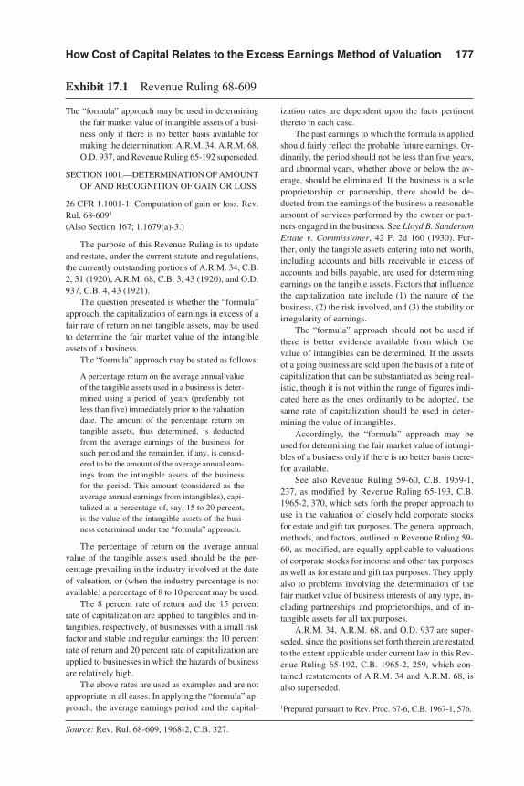
How Cost of Capital Relates to the Excess Earnings Method of Valuation 177
The “formula” approach may be used in determiningthe fair market value of intangible assets of a busi-ness only if there is no better basis available formaking the determination; A.R.M. 34, A.R.M. 68,O.D. 937, and Revenue Ruling 65-192 superseded.
SECTION 1001.—DETERMINATION OF AMOUNTOF AND RECOGNITION OF GAIN OR LOSS
26 CFR 1.1001-1: Computation of gain or loss. Rev.Rul. 68-6091
(Also Section 167; 1.1679(a)-3.)
The purpose of this Revenue Ruling is to updateand restate, under the current statute and regulations,the currently outstanding portions of A.R.M. 34, C.B.2, 31 (1920), A.R.M. 68, C.B. 3, 43 (1920), and O.D.937, C.B. 4, 43 (1921).
The question presented is whether the “formula”approach, the capitalization of earnings in excess of afair rate of return on net tangible assets, may be usedto determine the fair market value of the intangibleassets of a business.
The “formula” approach may be stated as follows:
A percentage return on the average annual valueof the tangible assets used in a business is deter-mined using a period of years (preferably notless than five) immediately prior to the valuationdate. The amount of the percentage return ontangible assets, thus determined, is deductedfrom the average earnings of the business forsuch period and the remainder, if any, is consid-ered to be the amount of the average annual earn-ings from the intangible assets of the businessfor the period. This amount (considered as theaverage annual earnings from intangibles), capi-talized at a percentage of, say, 15 to 20 percent,is the value of the intangible assets of the busi-ness determined under the “formula” approach.
The percentage of return on the average annualvalue of the tangible assets used should be the per-centage prevailing in the industry involved at the dateof valuation, or (when the industry percentage is notavailable) a percentage of 8 to 10 percent may be used.
The 8 percent rate of return and the 15 percentrate of capitalization are applied to tangibles and in-tangibles, respectively, of businesses with a small riskfactor and stable and regular earnings: the 10 percentrate of return and 20 percent rate of capitalization areapplied to businesses in which the hazards of businessare relatively high.
The above rates are used as examples and are notappropriate in all cases. In applying the “formula” ap-proach, the average earnings period and the capital-
ization rates are dependent upon the facts pertinentthereto in each case.
The past earnings to which the formula is appliedshould fairly reflect the probable future earnings. Or-dinarily, the period should not be less than five years,and abnormal years, whether above or below the av-erage, should be eliminated. If the business is a soleproprietorship or partnership, there should be de-ducted from the earnings of the business a reasonableamount of services performed by the owner or part-ners engaged in the business. See Lloyd B. SandersonEstate v. Commissioner, 42 F. 2d 160 (1930). Fur-ther, only the tangible assets entering into net worth,including accounts and bills receivable in excess ofaccounts and bills payable, are used for determiningearnings on the tangible assets. Factors that influencethe capitalization rate include (1) the nature of thebusiness, (2) the risk involved, and (3) the stability orirregularity of earnings.
The “formula” approach should not be used ifthere is better evidence available from which thevalue of intangibles can be determined. If the assetsof a going business are sold upon the basis of a rate ofcapitalization that can be substantiated as being real-istic, though it is not within the range of figures indi-cated here as the ones ordinarily to be adopted, thesame rate of capitalization should be used in deter-mining the value of intangibles.
Accordingly, the “formula” approach may beused for determining the fair market value of intangi-bles of a business only if there is no better basis there-for available.
See also Revenue Ruling 59-60, C.B. 1959-1,237, as modified by Revenue Ruling 65-193, C.B.1965-2, 370, which sets forth the proper approach touse in the valuation of closely held corporate stocksfor estate and gift tax purposes. The general approach,methods, and factors, outlined in Revenue Ruling 59-60, as modified, are equally applicable to valuationsof corporate stocks for income and other tax purposesas well as for estate and gift tax purposes. They applyalso to problems involving the determination of thefair market value of business interests of any type, in-cluding partnerships and proprietorships, and of in-tangible assets for all tax purposes.
A.R.M. 34, A.R.M. 68, and O.D. 937 are super-seded, since the positions set forth therein are restatedto the extent applicable under current law in this Rev-enue Ruling 65-192, C.B. 1965-2, 259, which con-tained restatements of A.R.M. 34 and A.R.M. 68, isalso superseded.
1Prepared pursuant to Rev. Proc. 67-6, C.B. 1967-1, 576.
Source: Rev. Rul. 68-609, 1968-2, C.B. 327.
Exhibit 17.1 Revenue Ruling 68-609
3953 P-17 8/29/02 2:25 PM Page 177
BASIC “EXCESS EARNINGS” VALUATION METHOD
The excess earnings method is a form of a capitalization method requiring sep-arate estimation of two capitalization rates. The reason for the two rates is that the in-come stream being capitalized is divided into two parts:
1. Income attributable to tangible assets. Less risky, lower required rate of return
2. Income attributable to intangible assets. More risky, generally higher requiredrate of return
The rule is simply that the weighted average of the two rates based on asset compo-nents (weighted at market values, of course) should approximately equal capitaliza-tion rates based on capital structure components estimated by methods discussed inthis book.
Conceptual Basis for the Method
The Guide to Business Valuations explains the concept of the excess earningsmethod:
The model for the excess earnings method computes the company’s equity value basedon the appraised value of tangible assets, plus an additional amount for intangible as-sets. A company’s tangible assets should provide a current return to the owner. Sincethere are risks associated with owning the company’s assets, the rate of return on thoseassets should be commensurate with the risks involved. That rate of return should be ei-ther the prevailing rate of return required to attract capital to that industry or an appro-priate rate above the risk-free rate. Any returns produced by the company above the rateon tangible assets are considered to arise from intangible assets. Accordingly, theweighted average capitalization rate for tangible assets and intangible assets should beequivalent to the capitalization rate for the entire company.2
Steps in Applying the Excess Earnings Method
The Guide to Business Valuations lists the steps required in implementing theexcess earnings method:
Step 1. Obtain the company’s financial statements. Apply the necessary GAAP(generally accepted accounting principles) and normalization adjustments(including adjustments for nonoperating assets). Recompute federal andstate income taxes, if necessary, based on normalized pretax earnings.
Step 2. Determine the value of the company’s net tangible assets.
Step 3. Determine a reasonable rate of return (as of the valuation date) on the ap-praised value of the company’s net tangible assets.
178 Other Topics Related to Cost of Capital
3953 P-17 8/29/02 2:25 PM Page 178
Step 4. Multiply the reasonable rate of return (Step 3) times the company’s nettangible asset value (Step 2). That amount is the “reasonable return” onthose assets.
Step 5. Subtract the calculated reasonable return (Step 4) from normalized netearnings (Step 1). That difference is the company’s “excess earnings.”
Step 6. Determine an appropriate capitalization rate (as of the valuation date) forthe company’s excess earnings, which are assumed to be attributable togoodwill or other intangible assets.
Step 7. Capitalize the excess earnings (divide excess earnings by the capitalizationrate).
Step 8. Add the amount computed in Step 7 and the value of the net tangible as-sets (Step 2).
Step 9. Perform “sanity checks” to determine the reasonableness of the value de-termined in Steps 1 through 8.
Step 10. Determine an appropriate value for any excess or nonoperating assets thatwere adjusted for in Step 1. If applicable, add the value of those assets to thevalue determined in Step 8. If asset shortages were identified in Step 1, de-termine if the value estimate should be reduced to reflect the value of suchshortages. If the normalized income statement was adjusted for identifiedasset shortages, it is not necessary to further reduce the value estimate.
Step 11. Determine if the value of the company computed in Step 8 should be ad-justed for a minority interest discount, discount for lack of marketability,or other discounts.3
A very good “sanity check,” as referred to in Step 9, is the cost of capital reason-ableness check outlined in this chapter.
Example of the Excess Earnings Method
For an example, we will use a company with 100% equity in its capital structure.This simplifies the example, although it works just as well in valuing overall investedcapital. As a practical matter, though, a majority of the companies to which this methodis applied have no long-term debt. We are reviewing an excess earnings method valu-ation prepared by Sam Shoveler for a company owner’s wife in a divorce proceeding.
The company is Kenny’s Landscaping Mob (KLM), a sole proprietorship withseveral years of history in a residential area primarily populated by employees of lum-ber, plywood, and papermill companies. Mill shutdowns are frequent, impactingKLM’s business, and there has even been talk of permanent closures. Kenny, now 45,supervises a high-turnover workforce whose members are paid a small fraction of thehourly rate that Kenny charges his clients for the gardening and landscaping workperformed. There is substantial client turnover, but Kenny advertises heavily andfinds new customers, at least when the mills are fully operating.
How Cost of Capital Relates to the Excess Earnings Method of Valuation 179
3953 P-17 8/29/02 2:25 PM Page 179
To illustrate a simple valuation of KLM by the excess earnings method, we willmake five assumptions:
1. An appraiser accredited by the American Society of Appraisers in Machinery andEquipment Appraisal and with experience in landscaping and gardening equip-ment has appraised KLM’s tangible assets on a value-in-use basis at $200,000.
2. Shoveler has determined that a reasonable rate of return on the company’s nettangible assets is 8%.
3. Shoveler has also determined that an appropriate capitalization rate for the com-pany’s excess earnings is 20%.
4. Normalized net cash flow for KLM, after reasonable compensation to Kenny, is$50,000 per year.
5. Because Kenny is always scrambling for both customers and workers, and be-cause the community’s industrial base is flat at best, growth in net cash flow isexpected to be only at the rate of inflation, estimated at 3%.
Shoveler’s summary of the excess earnings method of valuation of KLM is:
Tangible asset value $200,000Net cash flow $50,000Required return on tangible assets: 0.08 × $200,000 16,000———–Return attributable to intangible assets $34,000Intangible asset value (capitalized excess earnings)
$34,000 ÷ 0.20 170,000———––Total value of KLM $370,000———––———––
COST OF CAPITAL REASONABLENESS CHECK
The cost of capital reasonableness check is a fairly simple two-step process:
Step 1. Estimate a reasonable capitalization rate for the subject company by one ormore of the cost of capital estimation methods discussed in this book.
Step 2. Compute the weighted average capitalization rate (the weighted average ofthe returns on tangible assets and excess earnings, the latter representingthe return on intangible assets) implied in the excess earnings valuation,and compare it with the capitalization rate estimate in Step 1.
If the results of Step 1 and Step 2 are close, this implies passing marks on one testof the reasonableness of the rates used in the excess earnings method. (The analystshould recognize, of course, that the weighted average of the excess earnings methodrates could have been close to the overall capitalization rate by accident, and that dif-ferent tangible asset values or cash flows could still produce an unreasonable result.)
180 Other Topics Related to Cost of Capital
3953 P-17 8/29/02 2:25 PM Page 180
Computing the Weighted Average Excess EarningsCapitalization Rate
Returning to the excess earnings method valuation, we see that the company’sestimated value of $370,000 was composed of $200,000 tangible asset value and$170,000 intangible asset value. Computing the relative weights of these asset values,we have:
Tangible assets $200,000 ÷ $370,000 = 54.1%Intangible assets $170,000 ÷ $370,000 = 45.9–—–
= 100.0%
Weighting the required rates of return on the tangible and intangible asset valuecomponents gives us:
Tangible asset value 0.541 × 0.08 = 0.043Intangible asset value 0.459 × 0.20 = 0.092——–Weighted asset-based capitalization rate = 0.135——–——–
Estimating a Build-up Model Capitalization Rate
For a very small company like KLM, the build-up method, presented in Chapter8, is usually the best method for estimating an equity capitalization rate. To implementthe build-up method, we will make four assumptions:
1. Risk-free rate. At the valuation date, 7.0%
2. Equity risk premium. Arithmetic average from SBBI Valuation Edition Yearbook,7.4%
3. Size premium. Ibbotson’s tenth decile size premium from SBBI Valuation Edi-tion Yearbook, 5.33%
4. Company-specific risk premium. The company is tiny compared with Ibbotson’stenth-decile New York Stock Exchange stocks. The company has high specificrisk because of lack of stability of customer base and economic vulnerability ofits customer base due to conditions in the industry on which it is dependent. Inaddition, there is a key person issue: How easily could Kenny be replaced? Al-though this decision is quite subjective, it seems conservative to add a specificrisk factor of 5.0%.
Adding up the pertinent factors gives us this discount rate:
Risk-free rate 7.00%Equity risk premium 7.40Size premium 5.33Company-specific premium 5.00Estimated KLM cost of equity (discount rate) 24.73%
How Cost of Capital Relates to the Excess Earnings Method of Valuation 181
3953 P-17 8/29/02 2:25 PM Page 181
We then subtract the estimated growth rate from the discount rate to get the es-timated capitalization rate:
Estimated Capitalization Rate for KLM Cash Flows
Discount rate 24.73%– Estimated long-term growth rate 3.00————————————— ——–= Estimated capitalization rate 21.73%——–——–
A 13.5% asset-based capitalization rate certainly is significantly different froma 21.73% capitalization rate based on capital structure components. If we divided the$50,000 cash flow by the 13.5% asset-based capitalization rate, we would, of course,get the excess earnings method value of $370,000 ($50,000 ÷ 0.135 ≅ $370,000).
If we divided the $50,000 by the 21.73% build-up method capitalization rate, wewould get an indicated value of $230,097 ($50,000 ÷ 0.2173 ≅ $230,097).
Which do you believe?
Discussion of the Example
Considering the risks involved, it is unlikely that anyone would pay $170,000 forthe blue sky (a colloquial term used loosely to refer to intangible assets) in KLM. Andit can be argued that the 21.73% capitalization rate is an already conservative capi-talization rate itself.
Obviously, the capitalization rates for tangible assets and excess earnings usedby Mr. Shoveler in his excess earnings exercise are considerably too low. Note thatthe asset appraisal assumes value in use. This is the value to an operating business,not a liquidation value. There appears to be plenty of risk associated with these tan-gible assets. Accordingly, one point over the risk-free rate is not nearly an adequaterisk premium. Capitalizing excess earnings at 20% implies that a buyer will pay forfive years of expected excess earnings (1 ÷ 0.20 = 5). Typically, buyers will pay thatimplied multiple only for a very stable customer base. The KLM customer base cer-tainly is not stable.
Obviously, this is an extreme example. Its purpose is merely to illustrate the me-chanics of using cost of capital as a reasonableness check on an excess earningsmethod valuation. However, there have been worse abuses. There are even people whothink that the 30-day U.S. Treasury-bill rate is a satisfactory return rate of the tangibleassets employed in a business. Watch out for such abuses!
VAGARIES OF THE EXCESS EARNINGS METHOD
Revenue Ruling 68-609 is not very specific on many points, such as how incomeis defined. Definitions of income other than net cash flow may require some adjustmentto the capitalization rate, as we illustrated its development.
182 Other Topics Related to Cost of Capital
3953 P-17 8/29/02 2:25 PM Page 182
The many vagaries of the excess earnings method have been explored at greatlength and are beyond the scope of this book.4 The purpose here is simply to show themechanics of demonstrating whether the weighted capitalization rate implied in anexcess earnings valuation is within a reasonable range.
SUMMARY
The excess earnings method uses two capitalization rates:
1. A required return on tangible assets
2. A rate at which to capitalize “excess earnings,” returns over and above amountsnecessary to support the tangible assets in a business
The position presented in this chapter is that the weighted average of these tworates (weighted at market value, of course) should be approximately equal to a com-pany’s capitalization rate (developed as discussed in this book). This chapter has il-lustrated the mechanics of how to make such a comparison.
To explore the many vagaries of implementing the excess earnings valuationmethod, readers are encouraged to avail themselves of the references listed in the notes.
Notes
1. See, for example, Jay E. Fishman, Shannon P. Pratt, J. Clifford Griffith, and Mark Wells,Guide to Business Valuations, 12th ed. (Fort Worth, TX: Practitioners Publishing Com-pany, 2001, updated annually in May), 7-28–7-40; Shannon P. Pratt, Robert F. Reilly, andRobert P. Schweihs, Valuing Small Businesses and Professional Practices, 3d ed. (NewYork: McGraw-Hill, 1998), Chapter 23, “The Capitalized Excess Earnings Method”;Shannon P. Pratt, Robert F. Reilly, and Robert P. Schweihs, Valuing a Business: TheAnalysis and Appraisal of Closely Held Companies, 4th ed. (New York: McGraw-Hill,2000), Chapter 13, “The Capitalized Excess Earnings Method.”
2. Fishman, Pratt, Griffith, and Wells, Guide to Business Valuations, 7-28. Copyright ©2002 by Practitioners Publishing Company. All rights reserved. Reproduced with per-mission from Guide to Business Valuations, Twelfth Edition (January 2002). For productinformation, phone 800-323-8724 or log onto www.ppcnet.com.
3. Ibid. at 7-28 to 7-29.4. See the preceding references plus “Practitioners Disagree Strongly on Excess Earnings
Methodology,” Shannon Pratt’s Business Valuation Update® (April 1997): 1–3. Thesereferences provide guidance on estimating rates of return on tangible and intangible assets,among other things.
How Cost of Capital Relates to the Excess Earnings Method of Valuation 183
3953 P-17 8/29/02 2:25 PM Page 183
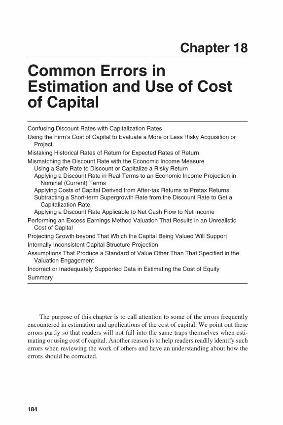
184
Chapter 18
Common Errors inEstimation and Use of Costof CapitalConfusing Discount Rates with Capitalization RatesUsing the Firm’s Cost of Capital to Evaluate a More or Less Risky Acquisition or
ProjectMistaking Historical Rates of Return for Expected Rates of ReturnMismatching the Discount Rate with the Economic Income Measure
Using a Safe Rate to Discount or Capitalize a Risky ReturnApplying a Discount Rate in Real Terms to an Economic Income Projection in
Nominal (Current) TermsApplying Costs of Capital Derived from After-tax Returns to Pretax ReturnsSubtracting a Short-term Supergrowth Rate from the Discount Rate to Get a
Capitalization RateApplying a Discount Rate Applicable to Net Cash Flow to Net Income
Performing an Excess Earnings Method Valuation That Results in an Unrealistic Cost of Capital
Projecting Growth beyond That Which the Capital Being Valued Will SupportInternally Inconsistent Capital Structure ProjectionAssumptions That Produce a Standard of Value Other Than That Specified in the
Valuation EngagementIncorrect or Inadequately Supported Data in Estimating the Cost of Equity
Summary
The purpose of this chapter is to call attention to some of the errors frequentlyencountered in estimation and applications of the cost of capital. We point out theseerrors partly so that readers will not fall into the same traps themselves when esti-mating or using cost of capital. Another reason is to help readers readily identify sucherrors when reviewing the work of others and have an understanding about how theerrors should be corrected.
3953 P-18 8/29/02 2:26 PM Page 184
CONFUSING DISCOUNT RATES WITH CAPITALIZATION RATES
The discount rate is the cost of capital, and it applies to all prospective economicincome. This includes all distributions and realized or readily realizable capital ap-preciation. The capitalization rate is a divisor applied to some particular economic in-come (e.g., earnings, cash flow, etc., for the latest 12 months, upcoming 12 months, orsome other period). Only when the expected level of economic income is constant inperpetuity are these two rates equal, other than by sheer coincidence.
Nevertheless, some analysts fall into the trap of using the discount rate (i.e., costof capital) as a capitalization rate. The opposite is also seen from time to time: the useof a capitalization rate to discount prospective cash flows or other expected economicincome to a present value.
The relationship between discount rates and capitalization rates is the subject ofChapter 4.
USING THE FIRM’S COST OF CAPITAL TO EVALUATE A MOREOR LESS RISKY ACQUISITION OR PROJECT
We have emphasized throughout this book that the cost of capital is market dri-ven and that it is a function of the investment, not the investor.
If an acquirer uses its own cost of capital to set an acquisition price by discountingthe expected cash flows of a riskier acquiree, then the result will be some increase in therisk of the acquiring company after the acquisition. This will result in an increase in thecompany’s overall risk and cost of capital, to which the market would be expected torespond by reducing the stock price. Decreases in acquirers’ stock prices as a result ofacquisitions are very common phenomena, although it is not possible to sort out the ex-tent to which this is a result of perceived overestimation of future cash flows or a mar-ket adjustment to the company’s cost of capital.
The same principle applies to internal capital budgeting and project selection asto acquisitions. If the project under consideration is more or less risky than the activ-ities of the company as a whole, then the expected cash flows from the project shouldbe evaluated by a correspondingly higher or lower discount rate. In deciding amongcompeting potential projects, an analyst should be certain to appropriately reflect therisk of each project in the discount rate applied to the respective project.
MISTAKING HISTORICAL RATES OF RETURN FOR EXPECTEDRATES OF RETURN
Remember, cost of capital is a forward-looking concept. Cost of capital is the ex-pected rate of return that the market requires to induce investment in a subject security.
Historical returns rarely are what investors expect in the future. Even if one wereto extrapolate historical returns into the future, one would be wrong most of the time.
Common Errors in Estimation and Use of Cost of Capital 185
3953 P-18 8/29/02 2:26 PM Page 185
The analyst should use historical returns only for guidance about what to expectin the future. If extrapolating historical returns into the future, the analyst should havesome basis for the assumption that the future will resemble the past on an extrapolatedbasis. This assumption should be articulated in the analyst’s report. Rarely are condi-tions in the economy, the industry, and the specific company comparable to what theywere in the past. The common error is for the analyst to naively assume that the futurewill fall somewhere near the line of extrapolation of the past. If this is, indeed, the as-sumption, the analyst should demonstrate that he or she has done the analysis and con-cluded that this will be true or that, at least, it is the best estimate of the future.
A related error is to take the recent average historical rates of return that havebeen achieved for an industry, often from a source of industry composite statisticssuch as the Risk Management Association’s (RMA) (formerly Robert Morris Asso-ciates) Annual Statement Studies, and to assume that this average is the expected re-turn required to attract investment in that industry. The returns actually achieved fora particular industry in recent past years may be well above or below the level of ex-pected return required to attract capital to the industry and certainly do not representa reliable indicator of the cost of capital. Furthermore, returns shown in sources suchas the RMA Annual Statement Studies are based on book values, whereas the relevantmeasure is return on market values. (The preceding discussion is not intended to to-tally eliminate all consideration of historical returns, such as a long-term average eq-uity risk premium.)
MISMATCHING THE DISCOUNT RATE WITH THE ECONOMICINCOME MEASURE
The most common type of error in application of the income approach to valua-tion is to use a discount or capitalization rate that is not appropriate for the definitionof economic income being discounted or capitalized. This general category of errorhas almost infinite variations. Those discussed in the next paragraphs are only a few.
Using a Safe Rate to Discount or Capitalize a Risky Return
Although not the most common version of the mismatching error, the use of a saferate to discount or capitalize a risky return certainly is one of the most egregious. On oc-casion, analysts erroneously discount a highly risky series of projected economic in-come by the U.S. Treasury-bill rate!
Applying a Discount Rate in Real Terms to an Economic IncomeProjection in Nominal (Current) Terms
In discounting or capitalizing, some analysts erroneously subtract the anticipatedinflation rate from the discount rate and then apply the adjusted discount rate to aneconomic income projection that includes inflation (and vice versa). It is noteworthy
186 Other Topics Related to Cost of Capital
3953 P-18 8/29/02 2:26 PM Page 186
that all the Ibbotson data are presented in nominal terms—that is, they include inflation.The most common way of performing the income approach to valuation in the UnitedStates and in other mature economies is to express the cash flows in nominal terms(including the effect of inflation) and use a nominal discount rate. In countries with hy-perinflation, it is more common to express expected cash flows in real terms and touse a discount rate not including expected inflation.
Applying Costs of Capital Derived from After-tax Returns toPretax Returns
Whether costs of capital are estimated by the build-up model, the Capital AssetPricing Model (CAPM), or the discounted cash flow (DCF) method, in all cases theyare returns realized after the payment of corporate-level income taxes. If the entitybeing valued is subject to entity-level income taxes, then it is inappropriate to apply thecost of capital estimated by those methods to pretax return flows.
As we go to press, three controversial U.S. Tax Court cases have been issued thatmany analysts believe are guilty of this error.1 The cases all involved S corporations,and the Tax Court applied discount rates developed on an after-tax basis to S corpo-ration earnings, which are pretax, on the theory that the corporation itself did not paythe taxes on the earnings. But someone had to pay the taxes. All S corporation statusdoes is pass through the tax liability to the owners and thus avoid double taxation. ButS corporation status does not avoid, or even defer, the obligation to pay the taxes onthe earnings.
Most public companies have a rather low payout ratio of dividends to earnings,if they even pay dividends at all. But in the case of S corporations, the earnings areall taxed to the owners, regardless of whether the earnings are actually distributed.We will undoubtedly hear more about this issue in the months and years to come.
Subtracting a Short-term Supergrowth Rate from the DiscountRate to Get a Capitalization Rate
Converting a discount rate to a capitalization rate involves subtracting an estimateof the long-term sustainable growth rate. Many companies expect high short-termgrowth that will tend to dampen over time. If the high short-term growth rate is sub-tracted from the discount rate, the proper capitalization rate will be understated, result-ing in overvaluation. In such circumstances, a two-stage or three-stage DCF valuationmodel usually will produce a more valid valuation than a straight capitalization model.
Applying a Discount Rate Applicable to Net Cash Flow to Net Income
One of the reviewers of this book said that this is the most common error he seesin practice.
Common Errors in Estimation and Use of Cost of Capital 187
3953 P-18 8/29/02 2:26 PM Page 187
Ibbotson data produces a discount rate that is applicable to net cash flow, whichusually is lower than net income. In such cases, the discount rate developed for netcash flow (or the capitalization rate derived by subtracting growth from the discountrate) would result in overvaluation if applied to net income.
If a consistent relationship exists between net cash flow and net income, then itis possible to adjust the discount rate by the proportion of net income to net cash flow.In a capitalization model, this is a reasonable approximation. However, very fewcompanies have an adequately consistent relationship between net cash flow and netincome to make this any more than an approximation.
PERFORMING AN EXCESS EARNINGS METHOD VALUATIONTHAT RESULTS IN AN UNREALISTIC COST OF CAPITAL
One very useful application of the cost of capital analysis is to do a sanity checkon the reality of a valuation performed by the excess earnings method, as discussedin the previous chapter.
In the excess earnings method, two capitalization rates are estimated:
1. A capitalization rate for tangible assets
2. A capitalization rate for excess earnings (return over and above the amount re-quired to support the company’s tangible assets)
The excess earnings method derives its capitalization rates by very differentmethods from those discussed earlier in this book. It is based on required returns tocategories of assets rather than on required returns to categories of capital. Never-theless, at the end of the day, the value as estimated by the excess earnings methodshould reflect a capitalization rate very similar to that which would be derived if wedeveloped a discount rate by any of the cost of capital estimation methods presentedin this book and subtracted a reasonable estimate of long-term sustainable growth.
The following is an example of such a sanity check:
Sanity Check. Is the overall equity capitalization rate approximately equal towhat you would expect using a build-up capitalization rate?
1. Analysis of overall equity cap rate using excess earnings method:Net cash flow to equity $270Divided by: indicated equity value $1,205——––Equals implied cap rate on equity: 22.4%——––——––
($270 ÷ $1,205 = 22.4%)2. Build-up cap rate:
20-year government bond rate 7.0%Small stock equity risk premium (combined general
equity premium and small stock premium) 15.8%Specific risk premium for subject 5.0%——––
188 Other Topics Related to Cost of Capital
3953 P-18 8/29/02 2:26 PM Page 188
Total required rate of return (discount rate) 27.8%Less: expected sustainable growth rate 4.0%——––Equals cap rate applicable to net cash flow: 23.8%——––——––
According to the sanity check, the results of the excess earnings method seemreasonable. If we capitalize the $270 net cash flow to equity at 23.8%, we would havean indicated value of $1,134, compared with $1,205 achieved by the excess earningsmethod. This is a reasonable range of difference. If the results were significantly dif-ferent, we would reexamine all our calculations and assumptions.
In the above example, we dealt only with a capitalization rate for equity, becausemost of the data sources used to perpetrate this error show only returns to equity ratherthan returns to total capital. The excess earnings method, however, is used more oftento value controlling interests than minority interests. Consequently, the return to totalcapital, as measured by the weighted average cost of capital (WACC), is relevant, andthus the capitalization rate for overall invested capital also should be considered inthe reasonableness test.
This use of cost of capital as a reasonableness check for an excess earnings methodvaluation was the subject of Chapter 17. That example demonstrated a significantovervaluation by the excess earnings method.
PROJECTING GROWTH BEYOND THAT WHICH THE CAPITALBEING VALUED WILL SUPPORT
As businesses expand, they typically need additional working capital and capitalexpenditures to support the increased level of operations. One of the many advantagesof using net cash flow as the prospective economic income measure is that it forces theanalyst to explicitly consider these needs. Nevertheless, they often are underestimated.
When cost of capital is used for valuation, it values only the investment as of thevaluation date. The calculation of net cash flow allows for reinvestment for capital ex-penditures and additions to working capital necessary to support projected operations.However, if the projections being discounted will not be totally supported by the cap-ital expenditure and working capital allowances in the net cash flow projections, andadditional investment will be required to achieve those projected results, then the ex-isting investment will be overvalued.
Many analysts do not make adequate deductions for capital expenditures and ad-ditions to working capital. Analysts should be sure that these items bear a reasonable re-lationship to revenue, especially to revenue growth. A good idea is to project balancesheets as well as income statements. This helps to show potential asset deficiencies.
These items also should be examined when calculating the terminal value. Ifgrowth is assumed when calculating the terminal value, then capital expenditures fol-lowing the discrete projection period should necessarily exceed depreciation followingthe discrete projection period. Many analysts assume capital expenditures to equal de-preciation when estimating the terminal value, which results in overestimation of ex-pected net cash flow and overvaluation, where growth is expected.2
Common Errors in Estimation and Use of Cost of Capital 189
3953 P-18 8/29/02 2:26 PM Page 189
INTERNALLY INCONSISTENT CAPITAL STRUCTUREPROJECTION
Methods using weighted average cost of capital and betas adjusted for leveragerequire projections about the subject company’s capital structure. These projectedcapital structures are on the basis of market value. Analysts often assume a capitalstructure in the process of estimating a market value of equity, and the resulting esti-mated market value of equity makes the capital structure, at the estimated marketvalue, different from that which was assumed.
In such cases, the projected capital structure has to be adjusted and the processiterated until the estimated market value of equity results in a capital structure con-sistent with that which is projected in estimating the cost of capital.
Even worse, of course, is to not even estimate a market value capital structure butsimply to use book value. If the company is earning good returns, then the marketvalue of equity is likely to exceed book value. This is true not only for the subjectcompany but also for peer companies that may be used to estimate an industry-averagecapital structure. If the market value of equity is understated, then the assumed pro-portion of low-cost debt in the capital structure will be too high. This will result in anunderstatement of the WACC and an overstatement of value.
Chapter 7 (WACC) addresses estimating capital structure by the iterative process,and Appendix E illustrates using the iterative process in the context of CAPM.
ASSUMPTIONS THAT PRODUCE A STANDARD OF VALUEOTHER THAN THAT SPECIFIED IN THE VALUATIONENGAGEMENT
A common error is to project a capital structure other than the company’s actualcapital structure (thereby deriving a weighted average cost of capital different from thecompany’s actual WACC) when the standard of value is fair market value on a mi-nority basis. If an acquirer were to use its own WACC, then the implied result wouldbe investment value to that acquirer instead of fair market value. Moreover, if the eq-uity ownership interest is a minority interest, the holder could not force a change incapital structure.
Another enormous assumption that would lead to investment value rather thanfair market value would be to inject the benefits of synergies into the projected cashflow stream. This would produce the value to a particular buyer who could take ad-vantage of the synergies, rather than a hypothetical buyer.
INCORRECT OR INADEQUATELY SUPPORTED DATA INESTIMATING THE COST OF EQUITY
The first mistake sometimes made in this category is to mismatch the risk-freerate with the equity risk premium. Ibbotson has equity premiums series that attachto 30-day Treasury-bill maturities, five-year Treasury-note maturities, and 20-year
190 Other Topics Related to Cost of Capital
3953 P-18 8/29/02 2:26 PM Page 190
Treasury-bond maturities. The equity risk premium should be selected to match oneof those maturities.
Ibbotson’s Stocks, Bonds, Bills and Inflation Valuation Edition Yearbook speci-fies the range for each of the size premia, and these vary from year to year. The sizeis measured in terms of market value of common equity capital. The size premiumdecreases as the market value increases. Mismatching the company size to the com-pany size premium can either understate or overstate the equity risk premium and there-fore understate or overstate value.
Another common error is inadequate support for the company-specific risk pre-mium. Within the CAPM, a portion of the company-specific risk may be captured inbeta. Certainly major portions of the company-specific risk are captured in the sizepremium. The remaining company-specific premium is totally a matter of the analyst’sjudgment. It should be based on quantitative and/or qualitative analysis, which shouldbe detailed in the report. The company-specific risk premium should be as small aspossible—sometimes we see 10 percentage points in the company-specific risk pre-mium, and that, depending on the company and the industry, is normally too much.Ten points would push the discount rate close to a venture capital or start-up companyrate. In any case, the company-specific risk premium should be supported with a verystrong narrative.
SUMMARY
Cost of capital is one of the most critical components in valuation, capital bud-geting, and other financial decision making. There are many ways to err in both esti-mating the cost of capital and applying it in practice. The errors regularly seen inactual practice are prolific. Some of the major areas that require careful considerationinclude:
• Properly distinguishing between discount rates and capitalization rates• Making sure that the data supporting discount and capitalization rates represent
expected returns (current market-required returns), not past returns that do not rep-resent future expectations
• Making sure that the discount or capitalization rate used matches the definition ofexpected returns being discounted or capitalized
• Making sure that the implied weighted capitalization rate used in an excess earn-ing valuation procedure is reasonably close to capitalization rates developed bythe cost of capital estimation methods discussed in this book
• Being careful that projected returns being discounted or capitalized can be achievedwithout having to dilute the existing capital with additional outside capital
• Being sure that capital structure assumptions fully reflect the market values of thecapital structure components
• Being sure that valuation results are estimated consistently with the definition ofvalue specified in the valuation assignment
• Making sure that the cost of equity is calculated correctly and supported adequately
Common Errors in Estimation and Use of Cost of Capital 191
3953 P-18 8/29/02 2:26 PM Page 191

Avoid all of these traps and you get a gold star! More important, your company andyour clients will be well served, and your cost of capital work should withstand rig-orous scrutiny.
Notes
1. Gross v. Commissioner, T.C. Memo 1999-254, 78 T.C.M. (CCH) 201 (U.S. Tax Ct. 1999),affirmed, 272 F.3d 333 (6th Cir. 2001); Estate of Heck v. Commissioner, T.C. Memo 2002-34, 83 T.C.M. (CCH) 1181 (U.S. Tax Ct. 2002); Estate of Adams v. Commissioner, T.C.Memo 2002-80 (U.S. Tax Ct. 2002).
2. For a good discussion of this common error, see Gilbert E. Matthews, “Cap X = Depreci-ation Is Unrealistic Assumption for Most Terminal Values,” Shannon Pratt’s Business Val-uation Update® (March 2002): 1–3.
192 Other Topics Related to Cost of Capital
3953 P-18 8/29/02 2:26 PM Page 192
193
Chapter 19
Cost of Capital in the CourtsCost of Capital in Shareholder DisputesCost of Capital in the Tax CourtCost of Capital in Family LawCost of Capital in Bankruptcy Reorganizations
Setting Interest RatesValuation of Stock by the Income Approach
Cost of Capital Included in DamagesCost of Capital in Utility Rate-settingTaxicab Lease Rates
Summary
Cost of capital is getting ever-increasing attention in the courts within many con-texts. These include valuations for many judicial purposes, allowed rates of return asa component in rate-setting, and other applications.
This chapter touches briefly on many of the contexts in which many millions ofdollars can hinge significantly on the court’s determination of the relevant cost of cap-ital. For each context, we have cited one or more cases that are typical of contempo-rary court deliberations on the subject.
COST OF CAPITAL IN SHAREHOLDER DISPUTES
Delaware traditionally has been the case law trendsetter on shareholder disputes.A landmark Delaware Supreme Court case in 1983 reversed a lower court case becauseit did not consider future earnings projections. The court made the point that a deter-mination of fair value (the statutory standard of value in Delaware, as well as in mostother states, for dissenting stockholder actions) “must include proof of value by anytechniques or methods which are generally considered acceptable in the financialcommunity.”1
Since that time, Delaware courts have increasingly embraced the discountedcash flow (DCF) method of valuation. In a 1997 case, the Delaware Chancery Courtcharacterized the DCF method as “increasingly the model of choice for valuations inthis Court.”2
In a typical case before the Delaware Supreme Court, both experts used the DCFmethod as well as other methods. The court rejected the other methods and focused
3953 P-19 8/29/02 2:26 PM Page 193
on the DCF method. The court accepted one expert’s Capital Asset Pricing Model(CAPM) for the cost of equity capital, with minor modifications to the beta (“[T]hebeta employed shall be based on the average beta of [the subject company’s] compa-rable companies.”) The court made some minor adjustments to the cash flow projec-tions because “it was apparent by the date of the merger [the effective valuation date]that [the subject company] would have a very difficult time meeting this projection.”Both experts used market multiples for their terminal values. The court accepted themultiple of the expert who had “convincingly demonstrated the appropriateness of[his] selection of [comparable companies].”3
However, in another case before the Delaware Court of Chancery, both expertsused the DCF method, with one using a 12% discount rate and the other an 18% dis-count rate. The court determined that the difference between the experts’ discount rateswas “attributable primarily to their different estimates of [the subject company’s] costof equity capital, and their different assumptions of the company specific risks con-fronting [the subject company] at the time of the merger.” The court disagreed with cer-tain of the other assumptions applied by both of the parties’ experts. The court ofchancery ultimately concluded that it could not rely on the DCF valuation opinion of ei-ther party’s expert.
The Delaware Supreme Court affirmed, stating: “Similarly, by recognizing thediscounted cash flow model as one proper valuation technique, the Court of Chancerywas not required to use that methodology to make its own independent valuation cal-culation by either adapting or blending the factual assumptions of the parties’ experts.The ultimate selection of a valuation framework is within the Court of Chancery’sdiscretion.”4
COST OF CAPITAL IN THE TAX COURT
Both the Internal Revenue Service (IRS) and the U.S. Tax Court traditionally haveleaned more toward the market approach than the income approach. The reason ispartly because of language in Revenue Ruling 59-60, written before the developmentof modern capital market theory, which evolved in the 1960s. The market approachhas also been favored partly because of concern about possible manipulation of bothcash flow forecasts and discount rates in the DCF method. Nonetheless, as the DCFmethod has achieved greater utilization in the professional financial community, it hasalso achieved greater acceptance in the Tax Court.
In a 1985 case the IRS challenged income tax returns reflecting deductions for acompany’s contributions to the employee stock ownership trust at $61.35 per share,based on the fair market value estimated by an independent appraisal firm. The IRSasserted that the value was between $5.36 and $8.00 per share. The independent ap-praisal heavily emphasized earning power and dividend-paying capacity, whereas theIRS stressed net asset value (book value was $7.05 per share).
The court agreed with the emphasis on earning power and dividend-paying ca-pacity. The court was somewhat concerned “that the appraisal took into account a 20-year earnings projection” but thought it was “not unreasonable in light of past earnings
194 Other Topics Related to Cost of Capital
3953 P-19 8/29/02 2:26 PM Page 194
increases.” The court concluded that the only reasonable appraisal presented to it wasthe one at $61.35 per share.5
Yet the Tax Court has rejected the DCF method in cases where it believed thatthe model used by the expert was far too sensitive to minor changes in assumptions,such as the discount rate and/or the growth rate.6
The Tax Court also has been known to reach its conclusion by giving partialweight to a DCF method and partial weight to a market approach method. For exam-ple, one case gave 70% weight to the market method and 30% weight to the DCFmethod.7
One Tax Court judge, obviously very knowledgeable about CAPM, rejected tes-timony offered in the context of the DCF but gave the following critique of the testi-mony for the guidance of other appraisers:
Beta of 1.00 too low. Beta, a measure of systematic risk, is a function of the relationshipbetween return on an individual security and the return on the market as a whole. . . .However, because the betas for small corporations tend to be larger than the betas forlarger corporations, it may be difficult to find suitable comparables when valuing a small,closely held corporation. . . . [T]here are substantial differences in size and operations be-tween [the subject company] and the banks on the VL bank list [Value Line InvestmentSurvey (4th ed., Apr. 9, 1993)]; we do not believe that their betas are representative of thegreater business risks faced by [the subject company].
We do not believe that an investment in [the subject company], a small, single-location bank, whose earnings were susceptible to impending interest rate mismatchesand sluggish local economic conditions, presents the same systematic risk as an invest-ment in an index fund holding shares in 500 of the largest corporations in the UnitedStates. . . .8
Failure to add small stock premium. Although [the witness] cited Ibbotson as hissource for equity risk premium, in his initial report he ignored a crucial aspect of the Ib-botson approach to constructing a cost of capital—the small stock premium. In his rebut-tal report, [the witness] unsuccessfully tried to persuade us that the small stock premiumis not supported by financial theory, characterizing the risk associated with a firm’s sizeas unsystematic risk, for which the market does not compensate. The relationship be-tween firm size and return is well known. Size is not an unsystematic risk factor andcannot be eliminated through diversification. “On average, small companies have higherreturns than large ones.” Ibbotson at 125. . . . [I]t has been found that the greater risk ofsmall stocks is not fully reflected by CAPM, in that actual returns may exceed those ex-pected based on beta. . . . Consequently, when calculating a cost of capital under CAPMon a small stock . . . , it is appropriate to add a small stock premium to the equity riskpremium, to reflect the greater risk associated with an investment in a small stock incomparison to the large stocks from which the equity-risk premium is calculated. Basedon [the subject company’s] size, a microcapitalization equity size premium of 3.6 per-cent should have been added. See Ibbotson at 161. . . .9
Failure to account for unsystematic risk. [B]ecause CAPM assumes that an investorholding a diversified portfolio will encounter only systematic risk, the only type of riskfor which an investor can be compensated is systematic or market risk, which representsthe sensitivity of the future returns from a given asset to the movements of the marketas a whole [citing Brealey & Myers, Principles of Corporate Finance 137–138, 143–144(4th ed. 1991); Pratt et al., Valuing a Business 166 (3rd ed. 1996)]. . . .
Cost of Capital in the Courts 195
3953 P-19 8/29/02 2:26 PM Page 195
[The witness] followed the principles of CAPM and did not make any provision for[the subject company’s] unsystematic risk, based on the assumption that such risk wasdiversifiable. . . . [R]espondent and [the witness] have overlooked the difficulties in di-versifying an investment in a block of stock they argued is worth approximately $8.94million. Construction of a diversified portfolio that will eliminate most unsystematicrisk requires from 10 to 20 securities of similar value. See Brealey & Myers, supra at137–139. Thus, proper diversification of an investment in the [the subject company]shares owned by petitioner, as valued by respondent, would require a total capital in-vestment of at least $89 million. We do not think the hypothetical buyer should be lim-ited only to a person or entity that has the means to invest $89 million in Peoples and aportfolio of nine other securities. . . .10
In another case, a witness added a small stock premium applicable to companiesmuch smaller than the subject company. For this reason, the court rejected that wit-ness’s cost of equity developed by the CAPM model and accepted the cost of equitycapital developed by the opposing witness, also by the CAPM model.11
The court rejected the DCF model for a small company in another case becauseit did not believe that CAPM and the WACC were “the proper analytical tools tovalue a small, closely held corporation with little possibility of going public.”12
Another case rejected the conclusion of a witness because he failed to apply asmall stock premium and used too low a beta:
Respondent relies on an article by Bajaj & Hakala, “Valuation for Smaller CapitalizationCompanies,” published in Financial Valuation: Business and Business Interests, ch. 12A(Hanan & Sheeler ed. 1998), for the proposition that there is no small-stock premium.We find [petitioner’s expert’s] analysis to be more persuasive.”
[Respondent’s expert] testified that it is appropriate to use the Ibbotson Associatesdata from the 1978–92 period rather than from the 1926–92 period because small stocksdid not consistently outperform large stocks during the 1980’s and 1990’s. We give lit-tle weight to [respondent’s expert’s] analysis. [He] appeared to selectively use data thatfavored his conclusion. He did not consistently use Ibbotson Associates data from the1978–92 period; he relied on data from the 1978–92 period to support his theory thatthere is no small-stock premium but used an equity risk premium of 7.3 percent from the1926–92 data (rather than the equity risk premium of 10.9 percent from the 1978–92 pe-riod). If he had used data consistently, he would have derived a small stock premium of5.2 percent and an equity risk premium of 7.3 percent using the 1926–92 data, ratherthan a small-stock premium of 2.8 percent and an equity risk premium of 10.9 percentusing the 1978–92 data.
We conclude that [petitioner’s expert] appropriately applied a small-stock premiumin valuing the [subject company’s] stock.13
In the same case, another issue in the income approach was the petitioner’s ex-pert’s build-up method versus the respondent’s expert’s CAPM method. Respondent’sexpert lowered his equity discount rate by multiplying it by a beta of 0.7. Judge Colvinstated the following:
We disagree with [respondent’s expert’s] use of a .7 beta because [the subject company]was a small, regional company, had customer concentrations, faced litigation and envi-
196 Other Topics Related to Cost of Capital
3953 P-19 8/29/02 2:26 PM Page 196
ronmental claims, had inadequate insurance, was not publicly traded, and had never paida dividend. A beta . . . can only be correctly estimated on the basis of the betas of com-parable publicly traded companies. . . . [Respondent’s expert] stated that he selected thebeta based on a review of comparable companies. However, he did not identify thesecomparable companies or otherwise give any reason for his use of a .7 beta. We believe[his] use of a .7 beta improperly increased his estimate of the value of the [subject com-pany’s] stock.14
As we go to press, three cases involving S corporations recently were decided.Since S corporation earnings are pretax, many appraisers valuing S corporation stockeither tax-affect the earnings (apply hypothetical taxes as if they were a C corporation)or increase the discount or capitalization rate by dividing the after-tax rate by 1 minusthe effective tax rate to derive a rate applicable to pretax earnings.15
The first such case was Gross v. Commissioner.16 One expert tax-affected the Scorporation earnings and the other did not. The Tax Court accepted the procedure ofnot tax-affecting the earnings. The case was appealed to the Sixth Circuit Court of Ap-peals, where the Tax Court decision was upheld by a two-to-one vote of the decidingjudges. The minority judge wrote a lengthy dissenting opinion.17
The next case was Estate of Heck v. Commissioner.18 In this case neither the ex-pert for the estate nor the expert for the IRS tax-affected the earnings or adjusted theafter-tax discount rate. Since both agreed, it was not an issue in the case, and the after-tax discount rate applied to the S corporation’s pretax earnings was allowed to stand.The expert for the taxpayer in that case was the same expert who testified for the IRSin the Gross case.
The last case before we went to press was Estate of Adams v. Commissioner.19 Inthe Adams case, one appraiser adjusted the capitalization rate (derived from Ibbotsonafter-tax discount rates) to apply to pretax earnings and the other did not. The Tax Courtaccepted the nonadjusted rate, resulting in an outcry from the professional business ap-praisal community. We have yet to see whether the Adams case will be appealed.
It is my opinion that these cases, if allowed to stand unchallenged and cited asprecedent, represent bad case law and a misinterpretation of fair market value. Taxeson S corporation earnings have to be paid. Denying tax-affecting of the earnings lim-its the pool of potential buyers to nontaxable entities. I believe that we will see somemodification of these results in appeals of these cases or in future cases.
COST OF CAPITAL IN FAMILY LAW
Cost of capital is getting increasing attention in family law courts as those courtsare becoming more receptive to the DCF method of valuation of closely held busi-nesses for marital property divisions.
In a 1996 Ohio case, for example, the trial judge stated from the bench that theDCF method had never been used before within her family law jurisdiction. She waswilling to consider it, based on testimony that members of the professional financialcommunity would be likely to use the method in valuing a company of the particular
Cost of Capital in the Courts 197
3953 P-19 8/29/02 2:26 PM Page 197
type at issue in the case. Ultimately the court not only accepted the method but usedthe value indicated by the DCF method as its final conclusion of value. The case wasappealed and upheld.20 Other courts have similarly followed suit.21
Shannon Pratt’s Business Valuation Update® consistently reports family lawcases that recognize the DCF method.
COST OF CAPITAL IN BANKRUPTCY REORGANIZATIONS
Cost of capital arises in bankruptcy proceedings in at least two contexts:
1. Setting interest rates
2. Valuing companies or interests in companies by the income approach
Setting Interest Rates
The concept of the cost of capital as described in this book is recognized for thepurpose of setting interest rates in the case of a bankruptcy reorganization. For ex-ample, the Seventh Circuit Court of Appeals rejected a trustee’s notion that the in-terest rate a creditor should receive should be the Treasury-bill rate.
The court stated that the creditor was entitled to “indubitable equivalence of itsproperty interest, which means a stream of payments including interest that adds up tothe present value of its claim. . . . [T]he creditor must get the market rate of interest . . .for loans for equivalent duration and risk.”
The court then added: “To say that the lender is limited to its ‘cost of capital’ . . .is therefore to say that the lender is entitled to the market rate of interest, for that is whatits cost of capital is: the price it must pay to its own lenders, plus the costs of makingand administering loans, plus reserves for bad debts (that is, the anticipated rate of non-payment).”22
Another court of appeals case in a different circuit stated the same concept. Inconsidering a reorganization plan involving interest payments, it stated that the issueis whether the interest rate provides the plaintiffs with the “present value” of theirclaims. The court explained: “ ‘Present value’ is a market rate concept, determined bythe use of an interest rate which fairly compensates the creditor for not receiving theamount of its secured claim upon confirmation of the debtor’s plan.”
The same court added, “[A]n entity forced to delay payment that it is entitled toreceive is, in effect, extending a loan.” The court further stated: “[T]he purpose . . .is . . . ‘to put the secured creditor in an economic position equivalent to the one itwould have occupied had it received the allowed secured amount immediately.’ . . .[T]he appropriate rate of interest is ‘that which the secured creditor would charge, atthe effective data of the plan, for a loan similar in character, amount and duration tothe credit which the creditor would be required to extend under the plan’.”23
The preceding case quoted the Third Circuit’s case of first impression on thisissue, a frequently-quoted case. In effect, the case rejected use of the prime lendingrate and required a market rate for similar credits:
198 Other Topics Related to Cost of Capital
3953 P-19 8/29/02 2:26 PM Page 198
Some courts, including the bankruptcy court in the cases we are here reviewing, havesuggested a “cost of funds” theory which would determine present value by looking tothe creditor and the market in which the creditor borrows capital.
There is more involved, however, than the mere cost of funds. . . .It is only by acknowledging the coerced loan aspects of a cramdown and by com-
pensating the secured creditor at the rate it would voluntarily accept for a loan of simi-lar character,* amount and duration that the creditor can be placed in the same positionhe would have been in but for the cramdown.
We hold that the bankruptcy and district courts erred in utilizing the prime rate to de-termine whether the proposed plan, as required by [the bankruptcy code], provided forpayments to the creditor having a present value equal to the value of its allowed securedclaim. The appropriate interest rate for this purpose is the rate of interest currently beingcharged by the creditor in the regular course of its business for loans similar in charac-ter, amount and duration to the loan being coerced in the cramdown.24
* By a loan of “similar character” we mean a loan that the creditor regularly extends to otherdebtors who are not in bankruptcy but who are otherwise similarly situated to the debtor who isthe recipient of the loan coerced by the Chapter 13 proceeding and who are seeking the samekind of credit (e.g., auto loan, home equity loan, etc.).
The Fifth Circuit reached a similar conclusion in a case decided September 8,1997.25
A common issue is setting appropriate interest rates to establish present value in“cram down” situations. In these situations, the bankruptcy court, in effect, forces thecreditor to accept a new loan for the property rather than allowing the creditor to re-possess the secured property.
In a consolidated 1998 case,26 the debtors’ Chapter 13 plan proposed to provide a9% interest rate on the balances due the creditors on automobiles in the debtors’ pos-session. Both creditors maintained that a 9% rate was inadequate to provide them withan amount equal to the present value of their claims as required by the bankruptcy code.Both creditors argued that the appropriate capitalization rate should be based on the rateof interest they currently charge for similar loans in the region. According to the cred-itors, the appropriate rate should be 20.19% in one case and 21% in the other.
The court determined that any analysis of this issue necessarily begins with theTenth Circuit opinion of In re Hardzog.27 The Tenth Circuit held that “in the absenceof special circumstances, such as the market rate being higher than the contract rate,bankruptcy courts should use the current market rate of interest used for similar loansin the region.”
The debtors argued that the “current market rate of interest” should be some vari-ation on the “prime lending rate” or “prevailing market rate” as reflected, for exam-ple, in The Wall Street Journal. The creditors argued that the correct interpretation of“current market rate of interest,” as used in Hardzog, means the rate charged by theparticular or objecting creditor for similar loans in the region in the recent past.
Citing Hardzog, the court determined that “similar” loans means a loan that thecreditor regularly extends to other borrowers who are not in bankruptcy but who areotherwise similarly situated to the debtor. Thus, the court ordered that the appropri-ate rates for the debtors should be 20.1% and 21%, respectively.
Cost of Capital in the Courts 199
3953 P-19 8/29/02 2:26 PM Page 199
Another case that followed shortly thereafter articulated the same conclusion28:
The remaining matter for the Court to decide is the appropriate cram down discount, orinterest rate n1 for payment for Household on the secured portion of its claim under [thebankruptcy code]. Debtors’ Chapter 13 plan proposed to pay an interest rate of 10% onthe secured portion of Household’s claim, and Household objected to this interest rateas being insufficient. The testimony of the witness from Household indicated that basedon the Debtors’ credit history, Household’s current interest rate would be in a range be-tween 18.95% and 24.95%. Debtors’ contract rate of interest is 22.95%. . . .
n1 For the sake of clarity, the Court will refer to “interest rate” though “discountrate” or “capitalization rate” may be more appropriate terms.
[The code] requires that a secured creditor receive payments that provide the presentvalue of the secured amount of its claim. In determining the appropriate interest rate, thisCourt must begin its analysis with Memphis Bank & Trust Co. v. Whitman, 692 F.2d 427(6th Cir. 1982). In Memphis Bank, the Sixth Circuit stated that it would be inappropri-ate to arbitrarily establish an interest rate for cram down under [the code], but instead“bankruptcy courts should use the current market rate of interest used for similar loansin the region.” Memphis Bank, 692 F.2d at 431. In making this determination, the Courtmust “assess interest on the secured claim for the present value of the collateral . . . inorder not to dilute the value of that claim through delay in payment. In effect, the law re-quires the creditor to make a new loan in the amount of the value of the collateral ratherthan repossess it, and the creditor is entitled to interest on his loan.” Memphis Bank, 692F.2d at 429.
The Sixth Circuit subsequently ruled that “the most equitable rate to establish in thistype of situation is the prevailing market rate of interest on similar types of securedloans at the time of allowance of the creditor’s claim and the confirmation of the planin bankruptcy with a maximum limitation on such rate to be the underlying contract rateof interest.” In re Colegrove, 771 F.2d 119, 123 (6th Cir. 1985). The use of the “currentmarket rate” of interest for cram down under . . . [the bankruptcy code], was alsoadopted in U.S. v. Arnold, 878 F.2d 925 (6th Cir. 1989). The Arnold court noted that thecontract interest rate maximum set forth in Colegrove was applicable only for fully se-cured creditors who were not required to write-down any portion of a loan. Arnold, 878F.2d at 929, 930. . . .
In light of Memphis Bank, Arnold and Colegrove, interest rates offered to low riskborrowers are not necessarily appropriate for cram down. . . . Other circuits have adopteda “coerced loan” approach, consistent with Memphis Bank, for determining appropriatecram down interest rate. . . . See General Motors Acceptance Corp. v. Jones, 999 F.2d63 (3d Cir. 1993); In re Hardzog, 901 F.2d 858 (10th Cir. 1990). The various approachesto determining the appropriate cram down interest rate were analyzed in a recent article,David G. Epstein, Don’t Go and Do Something Rash About Cram Down Interest Rates,49 Ala. L.Rev. 435 (1998):
Accordingly, in applying “value, as of the effective date of the plan,” bankruptcycourts should endeavor to leave the secured creditor as well off as if it had beenpaid the amount of its secured claim in cash. The cram down interest rate shouldreflect what the secured creditor would have earned had it taken that cash andreinvested it in loans with terms comparable to the terms proposed by thedebtors’ plan and with risks comparable to the risks presented by the debtor’snonpayment. . . .
200 Other Topics Related to Cost of Capital
3953 P-19 8/29/02 2:26 PM Page 200
This court finds that evidence of the relevant creditor’s recent loan rate for similarloans within the region will be instrumental for setting the proper cram down interestrate. . . .
In this case, Debtors presented no testimony or evidence concerning the market rateof interest that was available for borrowers with similar credit histories, but simply pro-posed an arbitrary interest rate of 10% for cram down. . . . Absolutely no support wasprovided for this rate, and the Court cannot accept such an arbitrary rate in light of Mem-phis Bank. The only evidence requiring an adjustment of the contract rate of interest, toaccurately reflect the current market interest rate for similar loans, came from House-hold’s witness who testified that the current market rate of interest for similar loansranged from 18.95% to 24.95%. The Court believes that the reduced risk associated withDebtors’ payments to the Chapter 13 trustee, and discharge of debts on completion oftheir Chapter 13 plan supports the use of the interest rate at the low end of Household’s“range,” and will set 18.95% as the interest rate to be paid on the secured portion ofHousehold’s claim under § 1325(a)(5)(B).
The above case contains references to many other cases espousing this position.
Valuation of Stock by the Income Approach
One case found flaws in the application of the discounted cash flow method29:
In discussing [the expert’s] application of the discounted cash flow method, the courtfound several flaws in [his] report and testimony:
• He failed to include information regarding additional working capital or capital expen-ditures that would be required for QSA to expand its business as he projected,
• He projected earnings without management input,• He failed to account for Mahoney’s salary as president and CEO of QSA, and• He assumed that QSA would terminate a distributorship contract, and further assumed
an estimated cost savings associated with this termination.30
The court ultimately rejected the above expert witness’s valuation and acceptedthe valuation of the opposing expert witness.
The issue in another interesting adversary proceeding31 was whether the transferof stock of Danbury Surgical Center, Inc. (DSC) and Bridgeport Surgical Center, Inc.(BSC) by debtors Googel and Sisti to the defendants Steinberg and Simons were fraud-ulent transfers under the bankruptcy code.
The transfer agreement recited the consideration as $100,000 for all of the stock.There was conflicting testimony regarding whether the release of debtors’ liability onthe centers’ financing was part of the consideration and whether additional consider-ation was promised to be paid “after the debtors’ financial troubles were over.”
The trustee’s expert used the discounted net cash flow method to value thestock, projected net cash flows for three years, used the industry average capitalstructure of 24% debt and 76% equity, computed a discount rate of 17.5%, and de-termined that DSC’s business enterprise value was $7,124,000. From this value he
Cost of Capital in the Courts 201
3953 P-19 8/29/02 2:26 PM Page 201
subtracted interest-bearing debt of $3,798,000, applied a 20% discount for lack ofmarketability, and applied an additional 5% discount for restrictions on voting rights.Based on Googel and Sisti’s ownership percentages of the total stock of DSC, thetrustee’s expert concluded that each debtor’s ownership interest was worth $349,100.He further tested the validity of his valuation by comparing the results with the valueof publicly traded surgical centers and with comparable centers that were tradedwithin a reasonable period before the subject transfer.
Defendants provided expert valuation testimony but did not independently ap-praise the value of the DSC stock. Instead, the expert provided a critical review of thetrustee’s expert’s appraisal. Defendant’s expert’s criticisms fell into three main areas.He testified that:
• [Trustee’s expert] failed to fully consider the impact of the Connecticut economy,which was in a recession;
• The discount rate and weighted average cost of capital [he] used did not account forthe “unsystematic risks” associated with valuing future cash flows of a small, privatelyowned, highly leveraged business; and
• [His] selection of a 20% discount for lack of marketability was too low—based upon anumber of discount studies a 35% discount for lack of marketability was appropriate.32
Defendant’s expert recommended changes in the calculations and concluded thateach debtor’s ownership interest in DSC was worth $126,000.
The court concluded that the trustee had not proven his claim of actual fraud be-cause the only evidence that additional consideration for the stock would be paid ata later date was the testimony of Googel. (It is of some interest that Googel testifiedby videotape due to his incarceration in federal prison for wire fraud, bank fraud, andimpeding administration of IRS laws.)
Regarding the trustee’s constructive fraud claim, the defendants conceded thatdebtors were insolvent at the time of the transfer. Therefore, the trustee needed toprove that debtors did not receive reasonably equivalent value for their stock. Basedon the expert valuation testimony, the court concluded that the debtors indeed did notreceive reasonably equivalent value for the DSC stock and the trustee therefore couldvoid the transfer as fraudulent.
The court generally credited the testimony of the trustee’s expert but adjusted hisvaluation conclusion by applying the 35% lack of marketability discount suggestedby defendant’s expert.
COST OF CAPITAL INCLUDED IN DAMAGES
In a District of Columbia (D.C.) case, the plaintiff appealed the district court’sdecision to award the cost of its lost capital, calculated on the basis of the totalamount of damages.
The D.C. Court of Appeals ruled:
It remains unclear whether prejudgment interest [interest from the time of the tort to thedate of court judgment] is available in a negligence action. Nonetheless . . . [i]n addition
202 Other Topics Related to Cost of Capital
3953 P-19 8/29/02 2:26 PM Page 202
to finding Williams negligent, the district court found that Straight had breached its con-tract with Smoot. Further, because Williams agreed to indemnify Straight in full, thecourt did not err by including the cost of capital in the damage award assessed againstWilliams—whether or not District of Columbia law allows a cost of capital award in anegligence action.
The court of appeals did, however, require an adjustment in the district court’scalculation of the time period for which portions of the cost of capital were awarded.The district court had awarded cost of capital on the full amount of the damagesthrough the last day of the trial. The court of appeals noted, however, that portions ofthe damages, such as increased insurance premiums and legal fees, were incurred overan extended period of time, and ordered a recalculation based on time of actual in-currence of damages.33
COST OF CAPITAL IN UTILITY RATE-SETTING
Many providers of essential services are subject to federal or state regulation in re-spect to the rates they can charge for their services. In setting rates, it is virtually uni-versally recognized that one of the costs the service provider is entitled to recover isits cost of capital. This generally is interpreted to mean its weighted average cost ofcapital, as discussed in Chapter 7.
This principle was articulated by the U.S. Supreme Court more than 50 yearsago:
The Supreme Court has stated that a just and reasonable rate should be “sufficient to as-sure confidence in the financial integrity of the enterprise, so as to maintain its credit andto attract capital”; the rate should also be “commensurate with returns on investments inother enterprises having corresponding risks.”34
The next quote from a case appealing a Federal Communications Commission(FCC) rate order is typical:
The FCC relied on “classic” DCF methodology, which assumes that the price of a shareof stock is equal to the present value of the cash flows the stock will generate. J. Bon-bright et al., Principles of Public Utility Rates 318 (2d ed. 1988).* These cash flows arein the form of dividends.** Because a dollar available now is worth more than a dollaravailable only later, the future cash flows must be reduced by a rate that reflects in-vestors’ opportunity costs, i.e., their required rate of return or discount rate, Id. Assum-ing that this discount rate and the growth rate of dividends both remain constant, onecalculates the price of the stock using the following formula: P = D/(r – g), where P isthe current price of the stock, D is the total dividend in the first year, r is the rate of re-turn, and g is the expected annual growth of dividends. Id.; see also A. Kolbe et al., TheCost of Capital: Estimating the Rate of Return for Public Utilities 53–54 (1984). Sinceregulatory commissions are interested in the rate of return, they rearrange the equationto solve for r: r = D/P + g.
Cost of Capital in the Courts 203
3953 P-19 8/29/02 2:26 PM Page 203
* The DCF method “has become the most popular technique of estimating the cost ofequity, and it is generally accepted by most commissions. Virtually all cost of capitalwitnesses use this method, and most of them consider it their primary technique.” Id.at 317–18.
** Cash flows also result from the ultimate sale of the stock. R. Brealey and S. Myers,Principles of Corporate Finance 49 (4th ed. 1991). However, the theory is that thenext investor will be willing to buy the stock at a price based on his estimate of futuredividends and the price at which he will be able to sell; so too the third investor andthe fourth, ad infinitum. The most basic form of the DCF model therefore assumesthat the stock is held forever. Bonbright et al., supra at 318. For a detailedexplanation, together with the mathematics, see 1.35
Similarly, a case challenging a Federal Energy Regulatory Commission (FERC)rate order supports the use of the Gordon Growth Model version of DCF analysis forestimating the cost of equity. Courts reviewing rate decisions generally will not re-quire the use of one method rather than another to estimate the cost of equity capitalbut will accept methods in common use in the financial community. The next excerptis typical of approval of regulatory methodology:
In fact, the Commission appears quite wedded to DCF analysis and to efficient market the-ory as its theoretical mainstay. In Montaup Electric Co., 38 FERC ¶ 61,252 (1987), for ex-ample, the Commission adopted the DCF methodology over risk premium analysis for aperiod of rapidly declining interest rates and reasoned that “a market-oriented analysissuch as a DCF analysis accounts for all risk factors perceived by investors.” Id. at 61,866.At about the same time as this court’s first remand, it published its third annual “genericDetermination of Rate of Return on Common Equity for Public Utilities,” in which it de-fended the use of the DCF methodology against attacks based on criticism of the EfficientMarket Hypothesis. Order No. 461, III FERC Regulations Preambles ¶ 30,722 (1987). Itdeclared enthusiastically, “The concept of an efficient market is astonishingly simple andremarkably well supported by the facts.”36
TAXICAB LEASE RATES
The City of Chicago Commissioner of Consumer Services retained a consultingfirm to recommend the rate of return on invested capital that Yellow Cab Companyshould be allowed to include in its maximum allowable lease rate for taxicabs. Thecommissioner adopted the consultant’s recommended rate of 14%, and Yellow Cabappealed to the U.S. District Court.
According to the court, “Based on extensive research and the concept of aweighted average cost of capital, which resulted in a 12 percent rate of return as-signed to the debt and a 20 percent rate of return given to the equity, [the consultant]determined that the maximum lease rates should afford a 14 percent rate of return.”
Yellow Cab’s actual cost of debt at the time was 7.25%, so the cost of capital wasbased on the risks and costs of the lease transaction, not on Yellow’s debt cost. Ingranting summary judgment for the defendants, the court stated, “Yellow Cab did notshow that the risk of the taxicab industry in Chicago entitled it to a rate of return ex-ceeding 20 percent.”37
204 Other Topics Related to Cost of Capital
3953 P-19 8/29/02 2:26 PM Page 204
SUMMARY
In matters such as valuation and allowed rates of return or interest rates, courts at-tempt to reflect the realities of financial decision making as practiced in the contem-porary financial environment. This includes the attempt to embrace modern capitalmarket theory in reaching determinations of the appropriate cost of capital in manycontexts.
These contexts include but are not limited to:
• Shareholders disputes
• Gift and estate tax valuations
• Marital property valuations
• Bankruptcy reorganizations
• Damage awards
• Rate-setting
• Lease rates
Courts are moving away from arbitrary cost of capital decisions and relying heav-ily on expert witnesses who use current market data in conjunction with the cost ofcapital estimation methods discussed in this book.
Notes
1. Weinberger v. UOP, Inc., 457 A.2d 701 (Del. 1983).2. Grimes v. Vitalink Comm. Corp., 1997 Del. Ch. LEXIS 124 (Del. Ch. 1997) (Oct. 1997
BVU).3. M.P.M. Enter., Inc. v. Gilbert, 731 A.2d 790 (Del. 1999).4. M.G. Bancorp., Inc. v. LeBeau, 737 A.2d 513 (Del. 1999).5. Las Vegas Dodge, Inc. v. United States, 1985 U.S. Dist. LEXIS 21577 (D. Nev. 1985).6. Morton v. Commissioner, T.C. Memo 1997-166, 73 T.C.M. (CCH) 2520 (U.S. Tax Ct.
1997) (June 1997 BVU).7. Estate of Freeman v. Commissioner, T.C. Memo 1996-372, 72 T.C.M. (CCH) 373 (U.S.
Tax Ct. 1996) (Oct. 1996 BVU).8. Estate of Hendrickson v. Commissioner, T.C. Memo 1999-278, 78 T.C.M. (CCH) 322
(U.S. Tax Ct. 1999) (Oct. 1999 J&L) (Oct. 1999 BVU).9. Id.
10. Id.11. Gross v. Commissioner, T.C. Memo 1999-254, 78 T.C.M. (CCH) 201 (U.S. Tax Ct.
1999) (Sept. 1999 J&L) (Sept. 1999 BVU), affirmed, 272 F.3d 333 (6th Cir. 2001) (Jan.2002 BVU).
12. Estate of Maggos v. Commissioner, T.C. Memo 2000-129, 79 T.C.M. (CCH) 1861 (U.S.Tax Ct. 2000) (July 2000 BVU).
13. Estate of Klauss v. Commissioner, T.C. Memo 2000-191, (U.S. Tax Ct. 2000) (July 2000BVU) (July 2000 J&L).
14. Id.
Cost of Capital in the Courts 205
3953 P-19 8/29/02 2:26 PM Page 205
15. Tax-affecting S corporation earnings is advocated by the IRS Valuation Training for Ap-peals Officers Coursebook (Chicago: CCH Incorporated, 1998), 7–12.
16. Gross v. Commissioner, T.C. Memo 1999-254, 78 T.C.M. (CCH) 201 (U.S. Tax Ct. 1999)(Sept. 1999 J&L) (Sept. 1999 BVU).
17. Gross v. Commissioner, 272 F.3d 333 (6th Cir. 2001). For an analysis of this discussion,see George Hawkins, “A Gross Result in the Gross Case Calls into Question Circum-stances in Which Tax Affecting Is Valid,” Shannon Pratt’s Business Valuation Update®
(Jan. 2002): 5–7 (Jan. 2002 BVU).18. Estate of Heck v. Commissioner, T.C. Memo 2002-34, 83 T.C.M. (CCH) 1181 (U.S. Tax
Ct. 2002) (March 2002 BVU).19. Estate of Adams v. Commissioner, T.C. Memo 2002-80 (U.S. Tax Ct. 2002) (May 2002
BVU).20. Sergi v. Sergi, 1996 Ohio App. LEXIS 3241 (Ohio Ct. App. 1996), appeal denied, 673
N.E.2d 147 (Ohio 1996) (Sept. 1996 BVU).21. Guiffre v. Baker, 1996 Ohio App. LEXIS 3673 (Ohio Ct. App. 1996) (Nov. 1996 BVU).22. Koopmans v. Farm Credit Serv., 102 F.3d 874 (7th Cir. 1996).23. Rankin v. DeSarno, 89 F.3d 1123 (3d Cir. 1996), certiorari denied, 519 U.S. 1108 (U.S.
Sup. Ct. 1997).24. General Motors Acceptance Corp. v. Jones, 999 F.2d 63 (3d Cir. 1993).25. Green Tree Fin. Serv. Corp. v. Smithwick, 121 F.3d 211 (5th Cir. 1997), rehearing de-
nied, 57 F.3d 1190 (D.C. Cir. 1991).26. In re Oglesby and Jones, 221 B.R. 515 (1998).27. In re Hardzog, 901 F.2d 858 (10th Cir. 1990).28. In re Glueck, 223 B.R. 514 (1998).29. “Bankruptcy Court Determines Fair Market Value Under Pennsylvania Judgment,”
Judges & Lawyers Business Valuation Update™ (May 2000): 7.30. In re Mahoney, 251 B.R. 748 (2000) (May 2000 J&L) (June 2000 BVU).31. In re Colonial Realty Co. 202 B.R. 185 (Bankr. D. Conn. 1996).32. “Stock Recipients Liable for Fraudulent Transfer Underpayment,” BVU (Jan. 1999): 10.33. Williams Enter., Inc. v. The Sherman R. Smoot Co., 938 F.2d 230 (D.C. Cir. 1991), re-
hearing denied, 57 F.3d 1190 (D.C. Cir. 1991).34. Federal Power Comm’n v. Hope Natural Gas Co., 320 U.S. 591 (U.S. Sup. Ct. 1944),
quoted in Illinois Bell Tel. Co. v. Federal Comm. Comm’n, 988 F.2d 1254 (D.C. Cir. 1993).35. Id.36. Tennessee Gas Pipeline Co. v. Federal Energy Regulatory Comm’n, 926 F.2d 1206 (D.C.
Cir. 1991).37. Yellow Cab Company v. City of Chicago, 938 F.Supp. 500, U.S. Dist. N.D. Ill. (Septem-
ber 10, 1996).
*Months in parentheses after case citations refer to the issue in which the case was abstracted,either in Shannon Pratt’s Business Valuation Update® (BVU), or in Judges & Lawyer’s Busi-ness Valuation Update™ (J&L) (now merged with BVU), as noted above. The full texts ofmost cases abstracted in either BVU or J&L are available online at www.BVLibrary.com.
206 Other Topics Related to Cost of Capital
3953 P-19 8/29/02 2:26 PM Page 206
207
Chapter 20
Cost of Capital in AdValorem Taxation
Carl R.E. Hoemke
Introduction to Ad Valorem TaxationSome Examples of Law That Promulgates the Definition of Income to DiscountGeneral Categories of Legislative Constraints Where Adjustments to the Cost of
Capital Are NecessaryCost of Capital in a Constant, Perpetual Cash Flow ScenarioDifferent Types of Adjustments
Multiplicative Income AdjustmentsLinear Income Adjustments: Constant Perpetual IncomeLinear Income Adjustments with a Growth VariantRandom Income VariantMultiplicative Value Adjustments
Other Adjustments to the Cost of CapitalEx Post and Ex Ante Risk PremiaSize PremiumIndustry Long-term Capitalization
Summary
Most people think of ad valorem as applicable only to real estate, but it applies in manybusiness valuation contexts as well. For example, there is a great deal of work for busi-ness appraisers (in which I have participated) among railroads, where the company asa whole is valued and that value allocated among the states through which the railroadruns. The most commonly used valuation method is the discounted cash flow (DCF)method, and a point or two difference in the discount rate can make millions of dollarsof difference in the resultant ad valorem taxes. Also, in some states, intangible assets arenot subject to ad valorem taxation.
Where value is assessed starting with the company as a whole, companies sometimessave millions of dollars in taxes by subtracting the value contributed by intangible as-sets. Also, I have undertaken assignments to quantify economic obsolescence for an in-dustrial plant, a task for which business appraisers may be more qualified than mostreal estate appraisers.
—Shannon Pratt
3953 P-20 8/29/02 2:26 PM Page 207
INTRODUCTION TO AD VALOREM TAXATION
Ad valorem taxation is a process in which government entities assess a tax orlevy on the value of property. Of the three basic types of taxes—the tax on wealth, thetax on income, and the tax on transactions, or excise taxes—the tax on wealth or prop-erty is the oldest and provides the revenue foundation for local governments. This taxis assessed per value, thus the Latin term ad valorem. Property value is determinedby the taxing jurisdiction, and a rate or levy is applied to the value for assessment.Proceeds are collected and used to fund services to the population of the taxing entity.These services may include police and fire protection, school funding, road funding,governmental administration, and others.
Many states have constitutional and statutory provisions that establish terms todefine the value to be used by the assessor for tax purposes. The terms full cash value,actual cash value, fair cash value, fair value in exchange, value in exchange, and trueand fair value are among those most commonly used. The courts have consistentlyinterpreted these terms as indicating the same kind of value, which is value in ex-change or value in the marketplace, normally termed market value. Therefore, we mayconsider that the basis of assessment is market value and that the assessor’s task is toestimate the market value of property. For this reason, there is a great need to estimateaccurately the value of property so that it can be fairly applied within its context.
The process of valuation has been described as an art form rather than a science.The appraiser’s final conclusion must be made by judgment to determine value. Theassessment of value therefore is limited by its tendency to be somewhat subjective; thusgovernmental authorities have attempted to make the process of assessment more ob-jective through policymaking. Some of the policies that have been created to simplifyand standardize the application of variables to value have served only to increase thecomplexity in the way cost of capital should be measured. This chapter identifies theadjustments to the cost of capital as applied in the income approach. The increasedcomplexity derives from the fact that standardization forces the analyst to deviatefrom preferred measurements of income.
There are three approaches to value:
1. Income
2. Cost
3. Market
Properties that are not frequently sold in the markets but have income streams arethe best candidates for the income approach to value. The income approach is a useful,although sensitive, appraisal tool. It is useful because, for most types of property, itis the most valid approach to value; it is sensitive, and therefore must be used with care,because any small original error will be compounded.
One of the parameters of concern in the income approach is the cost of capital.A basic assumption of the income approach is that people purchase property for theincome it will yield. A different way of stating the assumption is that the value of theproperty depends on the income it produces. In valuing income-producing property,
208 Other Topics Related to Cost of Capital
3953 P-20 8/29/02 2:26 PM Page 208
the valuation of an income stream is a function of the level of income being mea-sured. The level of income corresponds to ownership rights to the cash flows.
The preferred measure of return is net cash flow.1 There is certainly much dis-cussion and many theories on this measure, as previous chapters identify. Using thisreturn requires that the income to discount is the net cash flow income (see Chapter3 for definition). Both creditors and shareholders expect to be compensated for theopportunity cost of investing their funds in one particular business instead of in otherswith equivalent risk. In ad valorem taxation, the level of income to discount depends onthe limits placed on it by statutory requirements. Because of legislative constraintson the definition of income, adjustments must be made to the net cash flow return torender it comparable with the measure of income to discount.
SOME EXAMPLES OF LAW THAT PROMULGATES THEDEFINITION OF INCOME TO DISCOUNT
In many instances, limits or standards have promulgated the measure of income.For instance, if a governing body limits the definition of income to be discounted tothe earnings before depreciation, interest, and taxes (EBDIT), then the analyst mustrecognize these barriers and make opposing adjustments in the cost of capital to com-pensate for the recognition of taxes and capital expenditures. Another example: Ifstatutory requirements or practices require the subtraction of book depreciation fromEBDIT, then changes in the rate are necessary to match that specific level of incomecompared with net cash flow measurements. Statutory requirements can thus dramati-cally alter the cost of capital and leave the analyst with many adjustments to the stan-dard net cash flow cost of capital. It is essential that the analyst fully understand thecost of capital and its basis, then make any adjustments that make the cost of capitalcomparable with the income being measured.
GENERAL CATEGORIES OF LEGISLATIVE CONSTRAINTSWHERE ADJUSTMENTS TO THE COST OF CAPITAL ARENECESSARY
A good rule to use in making these adjustments is that any change made to the re-turn on net cash flow ultimately should result in a value that would have been arrivedat by measuring the present value of the net cash flow under no constraints. These area few situations in which adjustments to the cost of capital may be necessary:
• Cost of capital is used as a capitalization rate.
• Earnings are used as a proxy for free cash flow.
• Before-tax cash flow is used as the proxy for income.
• Adjustments are made for flotation costs.
• Adjustments are made for book value capital structure.
Cost of Capital in Ad Valorem Taxation 209
3953 P-20 8/29/02 2:26 PM Page 209
• Adjustments are made in the cost of capital for unaccounted capital expendituresin the cash flow.
COST OF CAPITAL IN A CONSTANT, PERPETUAL CASH FLOW SCENARIO
In its simplest form, the cost of capital is a function of a numerator income anda denominator value. It expresses the relationship of income to value.
The preferred level of income to discount is net cash flow. Net cash flow is theincome available for the equity investor after all obligations to other forms of capitalhave been satisfied. The discount rate applicable to this level of income is the rate thatis the subject of this book. If the expected net cash flows are constant and perpetual,then the discount rate (k) is simply the constant annual net cash flow (NCF) dividedby the present value (PV) of all future net cash flows.
Formula 20.1
For a constant and perpetual income (NCF):
Under these assumptions, any changes to the numerator will result in a direct and pro-portional change in k.
DIFFERENT TYPES OF ADJUSTMENTS
This section addresses how the changes in k influence the rate and how we mayadjust accordingly. The discussion covers three areas:
1. Income adjustments
2. Changes in relation to a percentage of value
3. Handling a combination of income and value adjustments
Each of these areas is elaborated in regard to both multiplicative and linear adjust-ments. A multiplicative adjustment is the application of a factor or percentage to thenumerator and/or denominator. Similarly, a linear adjustment is one in which a variableis added or subtracted to the numerator and/or denominator. Within the discussions ofmultiplicative and linear adjustments are analyses of the effects of changing variables.
Multiplicative Income Adjustments
The primary adjustment associated with a multiplicative income adjustment isthe effect of income taxes on the discount rate. Before-tax income is multiplied by an
kNCF
PV=
210 Other Topics Related to Cost of Capital
3953 P-20 8/29/02 2:26 PM Page 210
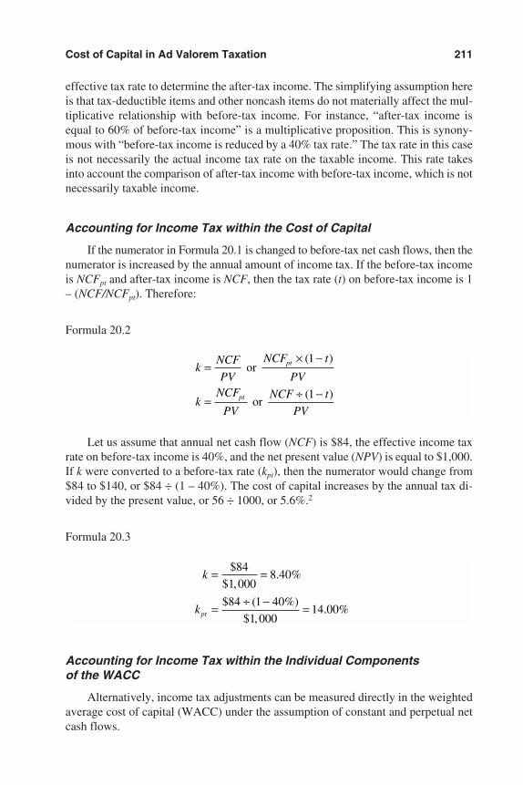
effective tax rate to determine the after-tax income. The simplifying assumption hereis that tax-deductible items and other noncash items do not materially affect the mul-tiplicative relationship with before-tax income. For instance, “after-tax income isequal to 60% of before-tax income” is a multiplicative proposition. This is synony-mous with “before-tax income is reduced by a 40% tax rate.” The tax rate in this caseis not necessarily the actual income tax rate on the taxable income. This rate takesinto account the comparison of after-tax income with before-tax income, which is notnecessarily taxable income.
Accounting for Income Tax within the Cost of Capital
If the numerator in Formula 20.1 is changed to before-tax net cash flows, then thenumerator is increased by the annual amount of income tax. If the before-tax incomeis NCFpt and after-tax income is NCF, then the tax rate (t) on before-tax income is 1– (NCF/NCFpt). Therefore:
Formula 20.2
Let us assume that annual net cash flow (NCF) is $84, the effective income taxrate on before-tax income is 40%, and the net present value (NPV) is equal to $1,000.If k were converted to a before-tax rate (kpt), then the numerator would change from$84 to $140, or $84 ÷ (1 – 40%). The cost of capital increases by the annual tax di-vided by the present value, or 56 ÷ 1000, or 5.6%.2
Formula 20.3
Accounting for Income Tax within the Individual Components of the WACC
Alternatively, income tax adjustments can be measured directly in the weightedaverage cost of capital (WACC) under the assumption of constant and perpetual netcash flows.
k
kpt
= =
= ÷ − =
$
$ ,. %
$ ( %)
$ ,. %
84
1 0008 40
84 1 40
1 00014 00
kNCF
PV
NCF t
PV
kNCF
PV
NCF t
PV
pt
pt
=× −
= ÷ −
or
or
( )
( )
1
1
Cost of Capital in Ad Valorem Taxation 211
3953 P-20 8/29/02 2:26 PM Page 211
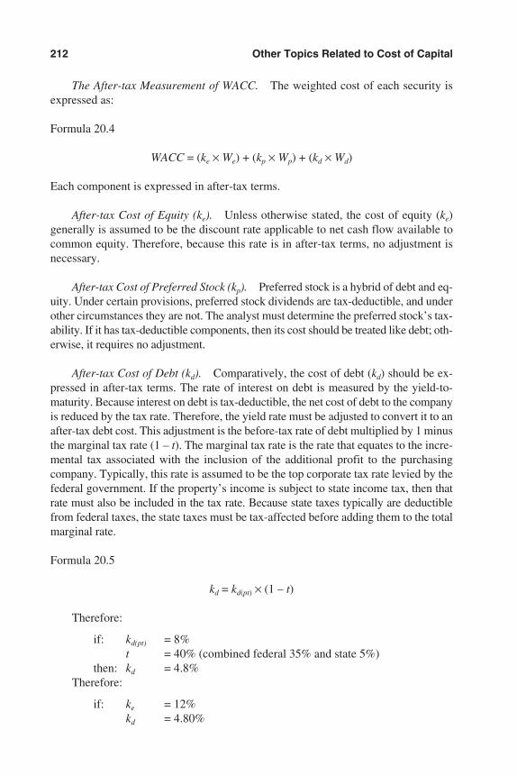
The After-tax Measurement of WACC. The weighted cost of each security isexpressed as:
Formula 20.4
WACC = (ke × We) + (kp × Wp) + (kd × Wd)
Each component is expressed in after-tax terms.
After-tax Cost of Equity (ke). Unless otherwise stated, the cost of equity (ke)generally is assumed to be the discount rate applicable to net cash flow available tocommon equity. Therefore, because this rate is in after-tax terms, no adjustment isnecessary.
After-tax Cost of Preferred Stock (kp). Preferred stock is a hybrid of debt and eq-uity. Under certain provisions, preferred stock dividends are tax-deductible, and underother circumstances they are not. The analyst must determine the preferred stock’s tax-ability. If it has tax-deductible components, then its cost should be treated like debt; oth-erwise, it requires no adjustment.
After-tax Cost of Debt (kd). Comparatively, the cost of debt (kd) should be ex-pressed in after-tax terms. The rate of interest on debt is measured by the yield-to-maturity. Because interest on debt is tax-deductible, the net cost of debt to the companyis reduced by the tax rate. Therefore, the yield rate must be adjusted to convert it to anafter-tax debt cost. This adjustment is the before-tax rate of debt multiplied by 1 minusthe marginal tax rate (1 – t). The marginal tax rate is the rate that equates to the incre-mental tax associated with the inclusion of the additional profit to the purchasingcompany. Typically, this rate is assumed to be the top corporate tax rate levied by thefederal government. If the property’s income is subject to state income tax, then thatrate must also be included in the tax rate. Because state taxes typically are deductiblefrom federal taxes, the state taxes must be tax-affected before adding them to the totalmarginal rate.
Formula 20.5
kd = kd(pt) × (1 – t)
Therefore:
if: kd(pt) = 8%t = 40% (combined federal 35% and state 5%)
then: kd = 4.8%Therefore:
if: ke = 12%kd = 4.80%
212 Other Topics Related to Cost of Capital
3953 P-20 8/29/02 2:26 PM Page 212
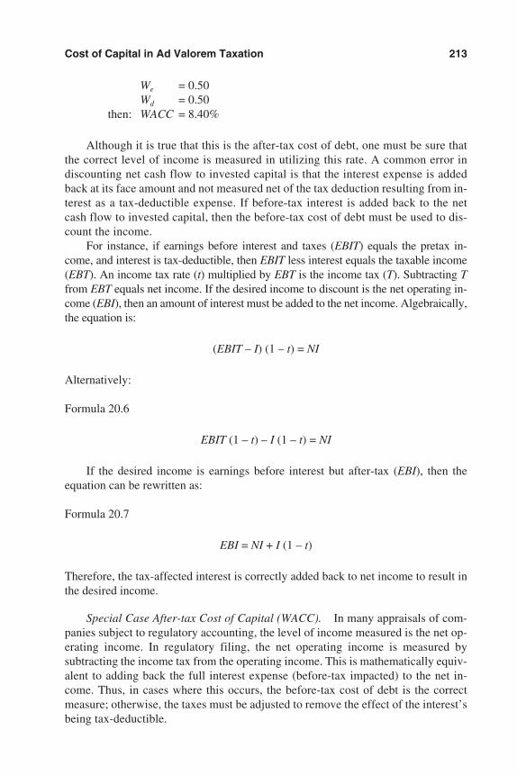
We = 0.50Wd = 0.50
then: WACC = 8.40%
Although it is true that this is the after-tax cost of debt, one must be sure thatthe correct level of income is measured in utilizing this rate. A common error indiscounting net cash flow to invested capital is that the interest expense is addedback at its face amount and not measured net of the tax deduction resulting from in-terest as a tax-deductible expense. If before-tax interest is added back to the netcash flow to invested capital, then the before-tax cost of debt must be used to dis-count the income.
For instance, if earnings before interest and taxes (EBIT) equals the pretax in-come, and interest is tax-deductible, then EBIT less interest equals the taxable income(EBT). An income tax rate (t) multiplied by EBT is the income tax (T). Subtracting Tfrom EBT equals net income. If the desired income to discount is the net operating in-come (EBI), then an amount of interest must be added to the net income. Algebraically,the equation is:
(EBIT – I) (1 – t) = NI
Alternatively:
Formula 20.6
EBIT (1 – t) – I (1 – t) = NI
If the desired income is earnings before interest but after-tax (EBI), then theequation can be rewritten as:
Formula 20.7
EBI = NI + I (1 – t)
Therefore, the tax-affected interest is correctly added back to net income to result inthe desired income.
Special Case After-tax Cost of Capital (WACC). In many appraisals of com-panies subject to regulatory accounting, the level of income measured is the net op-erating income. In regulatory filing, the net operating income is measured bysubtracting the income tax from the operating income. This is mathematically equiv-alent to adding back the full interest expense (before-tax impacted) to the net in-come. Thus, in cases where this occurs, the before-tax cost of debt is the correctmeasure; otherwise, the taxes must be adjusted to remove the effect of the interest’sbeing tax-deductible.
Cost of Capital in Ad Valorem Taxation 213
3953 P-20 8/29/02 2:26 PM Page 213
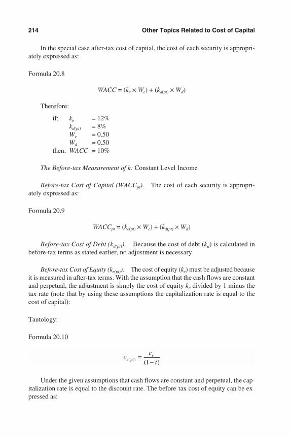
In the special case after-tax cost of capital, the cost of each security is appropri-ately expressed as:
Formula 20.8
WACC = (ke × We) + (kd(pt) × Wd)
Therefore:
if: ke = 12%kd(pt) = 8%We = 0.50Wd = 0.50
then: WACC = 10%
The Before-tax Measurement of k: Constant Level Income
Before-tax Cost of Capital (WACCpt). The cost of each security is appropri-ately expressed as:
Formula 20.9
WACCpt = (ke(pt) × We) + (kd(pt) × Wd)
Before-tax Cost of Debt (kd(pt)). Because the cost of debt (kd) is calculated inbefore-tax terms as stated earlier, no adjustment is necessary.
Before-tax Cost of Equity (ke(pt)). The cost of equity (ke) must be adjusted becauseit is measured in after-tax terms. With the assumption that the cash flows are constantand perpetual, the adjustment is simply the cost of equity ke divided by 1 minus thetax rate (note that by using these assumptions the capitalization rate is equal to thecost of capital):
Tautology:
Formula 20.10
Under the given assumptions that cash flows are constant and perpetual, the cap-italization rate is equal to the discount rate. The before-tax cost of equity can be ex-pressed as:
cc
te pte
( ) ( )=
−1
214 Other Topics Related to Cost of Capital
3953 P-20 8/29/02 2:26 PM Page 214
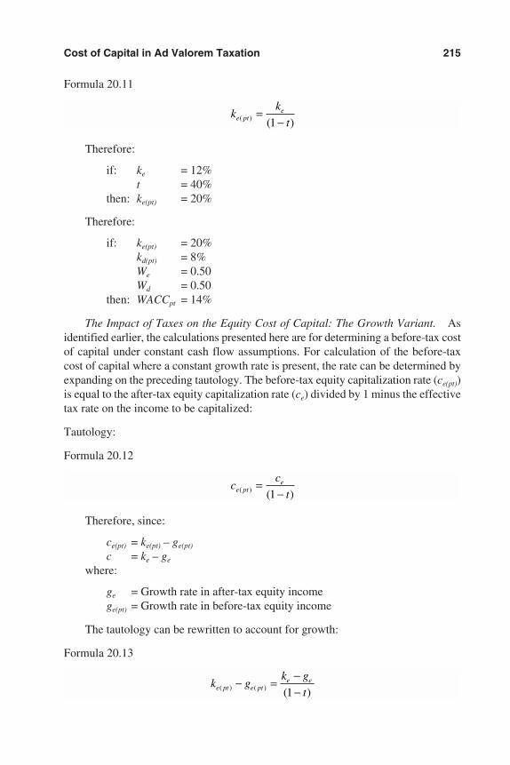
Formula 20.11
Therefore:
if: ke = 12%t = 40%
then: ke(pt) = 20%
Therefore:
if: ke(pt) = 20%kd(pt) = 8%We = 0.50Wd = 0.50
then: WACCpt = 14%
The Impact of Taxes on the Equity Cost of Capital: The Growth Variant. Asidentified earlier, the calculations presented here are for determining a before-tax costof capital under constant cash flow assumptions. For calculation of the before-taxcost of capital where a constant growth rate is present, the rate can be determined byexpanding on the preceding tautology. The before-tax equity capitalization rate (ce(pt))is equal to the after-tax equity capitalization rate (ce) divided by 1 minus the effectivetax rate on the income to be capitalized:
Tautology:
Formula 20.12
Therefore, since:
ce(pt) = ke(pt) – ge(pt)
c = ke – ge
where:
ge = Growth rate in after-tax equity incomege(pt) = Growth rate in before-tax equity income
The tautology can be rewritten to account for growth:
Formula 20.13
k gk g
te pt e pte e
( ) ( ) ( )− = −
−1
cc
te pte
( ) ( )=
−1
kk
te pte
( ) ( )=
−1
Cost of Capital in Ad Valorem Taxation 215
3953 P-20 8/29/02 2:26 PM Page 215
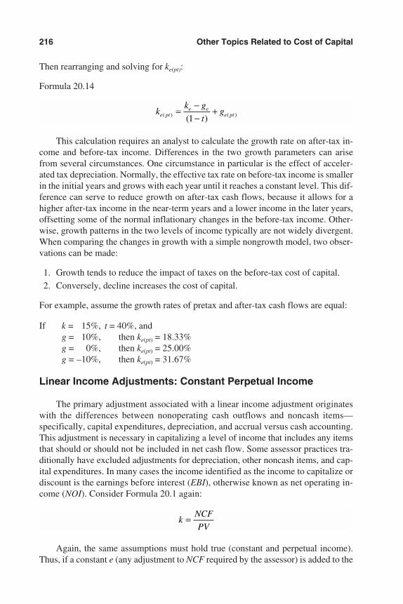
Then rearranging and solving for ke(pt):
Formula 20.14
This calculation requires an analyst to calculate the growth rate on after-tax in-come and before-tax income. Differences in the two growth parameters can arisefrom several circumstances. One circumstance in particular is the effect of acceler-ated tax depreciation. Normally, the effective tax rate on before-tax income is smallerin the initial years and grows with each year until it reaches a constant level. This dif-ference can serve to reduce growth on after-tax cash flows, because it allows for ahigher after-tax income in the near-term years and a lower income in the later years,offsetting some of the normal inflationary changes in the before-tax income. Other-wise, growth patterns in the two levels of income typically are not widely divergent.When comparing the changes in growth with a simple nongrowth model, two obser-vations can be made:
1. Growth tends to reduce the impact of taxes on the before-tax cost of capital.
2. Conversely, decline increases the cost of capital.
For example, assume the growth rates of pretax and after-tax cash flows are equal:
If k = 15%, t = 40%, andg = 10%, then ke(pt) = 18.33%g = 0%, then ke(pt) = 25.00%g = –10%, then ke(pt) = 31.67%
Linear Income Adjustments: Constant Perpetual Income
The primary adjustment associated with a linear income adjustment originateswith the differences between nonoperating cash outflows and noncash items—specifically, capital expenditures, depreciation, and accrual versus cash accounting.This adjustment is necessary in capitalizing a level of income that includes any itemsthat should or should not be included in net cash flow. Some assessor practices tra-ditionally have excluded adjustments for depreciation, other noncash items, and cap-ital expenditures. In many cases the income identified as the income to capitalize ordiscount is the earnings before interest (EBI), otherwise known as net operating in-come (NOI). Consider Formula 20.1 again:
Again, the same assumptions must hold true (constant and perpetual income).Thus, if a constant e (any adjustment to NCF required by the assessor) is added to the
kNCF
PV=
kk g
tge pt
e ee pt( ) ( )( )
= −−
+1
216 Other Topics Related to Cost of Capital
3953 P-20 8/29/02 2:26 PM Page 216
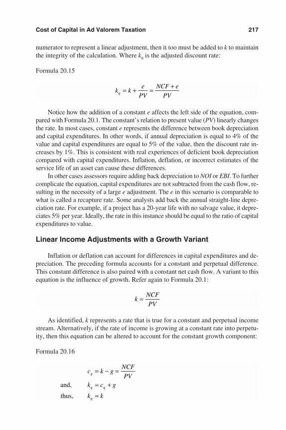
numerator to represent a linear adjustment, then it too must be added to k to maintainthe integrity of the calculation. Where kq is the adjusted discount rate:
Formula 20.15
Notice how the addition of a constant e affects the left side of the equation, com-pared with Formula 20.1. The constant’s relation to present value (PV) linearly changesthe rate. In most cases, constant e represents the difference between book depreciationand capital expenditures. In other words, if annual depreciation is equal to 4% of thevalue and capital expenditures are equal to 5% of the value, then the discount rate in-creases by 1%. This is consistent with real experiences of deficient book depreciationcompared with capital expenditures. Inflation, deflation, or incorrect estimates of theservice life of an asset can cause these differences.
In other cases assessors require adding back depreciation to NOI or EBI. To furthercomplicate the equation, capital expenditures are not subtracted from the cash flow, re-sulting in the necessity of a large e adjustment. The e in this scenario is comparable towhat is called a recapture rate. Some analysts add back the annual straight-line depre-ciation rate. For example, if a project has a 20-year life with no salvage value, it depre-ciates 5% per year. Ideally, the rate in this instance should be equal to the ratio of capitalexpenditures to value.
Linear Income Adjustments with a Growth Variant
Inflation or deflation can account for differences in capital expenditures and de-preciation. The preceding formula accounts for a constant and perpetual difference.This constant difference is also paired with a constant net cash flow. A variant to thisequation is the influence of growth. Refer again to Formula 20.1:
As identified, k represents a rate that is true for a constant and perpetual incomestream. Alternatively, if the rate of income is growing at a constant rate into perpetu-ity, then this equation can be altered to account for the constant growth component:
Formula 20.16
c k gNCF
PVk c g
k k
q
q q
q
= − =
= +
=
and,
thus,
kNCF
PV=
k ke
PV
NCF e
PVq = + = +
Cost of Capital in Ad Valorem Taxation 217
3953 P-20 8/29/02 2:26 PM Page 217
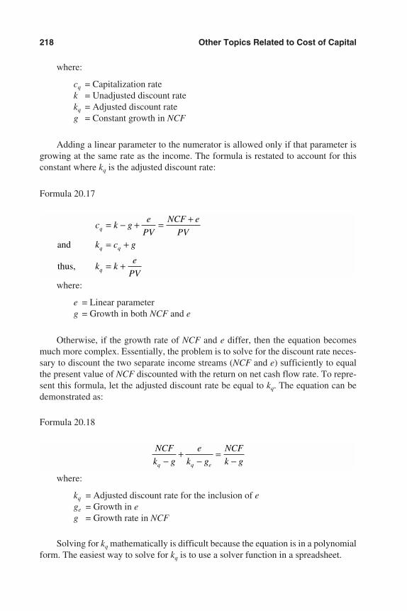
where:
cq = Capitalization ratek = Unadjusted discount ratekq = Adjusted discount rateg = Constant growth in NCF
Adding a linear parameter to the numerator is allowed only if that parameter isgrowing at the same rate as the income. The formula is restated to account for thisconstant where kq is the adjusted discount rate:
Formula 20.17
where:
e = Linear parameterg = Growth in both NCF and e
Otherwise, if the growth rate of NCF and e differ, then the equation becomesmuch more complex. Essentially, the problem is to solve for the discount rate neces-sary to discount the two separate income streams (NCF and e) sufficiently to equalthe present value of NCF discounted with the return on net cash flow rate. To repre-sent this formula, let the adjusted discount rate be equal to kq. The equation can bedemonstrated as:
Formula 20.18
where:
kq = Adjusted discount rate for the inclusion of ege = Growth in eg = Growth rate in NCF
Solving for kq mathematically is difficult because the equation is in a polynomialform. The easiest way to solve for kq is to use a solver function in a spreadsheet.
NCF
k g
e
k g
NCF
k gq q e−+
−=
−
c k ge
PV
NCF e
PVk c g
k ke
PV
q
q q
q
= − + = +
= +
= +
and
thus,
218 Other Topics Related to Cost of Capital
3953 P-20 8/29/02 2:26 PM Page 218
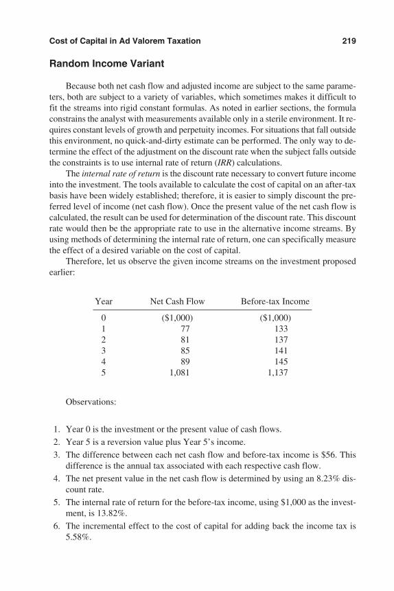
Random Income Variant
Because both net cash flow and adjusted income are subject to the same parame-ters, both are subject to a variety of variables, which sometimes makes it difficult tofit the streams into rigid constant formulas. As noted in earlier sections, the formulaconstrains the analyst with measurements available only in a sterile environment. It re-quires constant levels of growth and perpetuity incomes. For situations that fall outsidethis environment, no quick-and-dirty estimate can be performed. The only way to de-termine the effect of the adjustment on the discount rate when the subject falls outsidethe constraints is to use internal rate of return (IRR) calculations.
The internal rate of return is the discount rate necessary to convert future incomeinto the investment. The tools available to calculate the cost of capital on an after-taxbasis have been widely established; therefore, it is easier to simply discount the pre-ferred level of income (net cash flow). Once the present value of the net cash flow iscalculated, the result can be used for determination of the discount rate. This discountrate would then be the appropriate rate to use in the alternative income streams. Byusing methods of determining the internal rate of return, one can specifically measurethe effect of a desired variable on the cost of capital.
Therefore, let us observe the given income streams on the investment proposedearlier:
Year Net Cash Flow Before-tax Income
0 ($1,000) ($1,000)1 77 1332 81 1373 85 1414 89 1455 1,081 1,137
Observations:
1. Year 0 is the investment or the present value of cash flows.
2. Year 5 is a reversion value plus Year 5’s income.
3. The difference between each net cash flow and before-tax income is $56. Thisdifference is the annual tax associated with each respective cash flow.
4. The net present value in the net cash flow is determined by using an 8.23% dis-count rate.
5. The internal rate of return for the before-tax income, using $1,000 as the invest-ment, is 13.82%.
6. The incremental effect to the cost of capital for adding back the income tax is5.58%.
Cost of Capital in Ad Valorem Taxation 219
3953 P-20 8/29/02 2:26 PM Page 219
This process will return a rate equivalent to the before-tax discount rate. This is the de-sired method of calculating the true effect of taxes on the discount rate. Several thingsare occurring here that lead to a result on a before-tax basis. Generally, the reason forcalculating the IRR is that inconsistent growth rates between net cash flow and before-tax income are difficult to model in an easy-to-understand formula. Unfortunately, thedownside to this process is that it is more complex and a little more difficult to explain.
Multiplicative Value Adjustments
Ad Valorem Tax Addback
The most common multiplicative value adjustment in ad valorem assessment isthe addback of ad valorem taxes. Many assessors want to remove the historical bias re-sulting from prior valuations. Therefore, they may prefer to account for property taxwithin the discount rate. They do so by adding back to the discount rate the percent re-lationship of tax to market value. This adjustment is most similar to the linear adjust-ment in income. The difference is that the adjustment is a direct function of value. Inother words, if the value increases, the adjustment increases directly with the value,and vice versa. This can be demonstrated by the next formula:
Formula 20.19
where:
o = Percent of tax to value
And with the addition of a growth component (g), the formula expands to:
Formula 20.20
kq – g = k – g + othus, kq = k + o
The same formula can be used for any adjustment that is equal to a percentageof value. This holds true even in random changes in value. The only caveat is that thepercent relationship to value must remain constant. This adjustment is quite power-ful and easy to demonstrate, which is likely the reason for its popularity.
Flotation Costs
Another type of multiplicative value adjustment is flotation costs. Flotation costsoccur when new issues of stock or debt are sold to the public. The firm usually incurs
k k o PV PVo PV
PVk k o
q
q
= + × ÷ = ÷ ×
= +
( )( )1
thus,
220 Other Topics Related to Cost of Capital
3953 P-20 8/29/02 2:26 PM Page 220
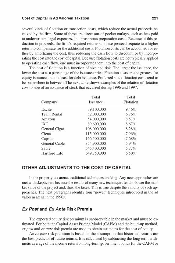
several kinds of flotation or transaction costs, which reduce the actual proceeds re-ceived by the firm. Some of these are direct out-of-pocket outlays, such as fees paidto underwriters, legal expenses, and prospectus preparation costs. Because of this re-duction in proceeds, the firm’s required returns on these proceeds equate to a higherreturn to compensate for the additional costs. Flotation costs can be accounted for ei-ther by amortizing the cost, thus reducing the cash flow to discount, or by incorpo-rating the cost into the cost of capital. Because flotation costs are not typically appliedto operating cash flow, one must incorporate them into the cost of capital.
The cost of flotation is a function of size and risk. The larger the issuance, thelower the cost as a percentage of the issuance price. Flotation costs are the greatest forequity issuance and the least for debt issuance. Preferred stock flotation costs tend tobe somewhere in between. The next table shows examples of the relation of flotationcost to size of an issuance of stock that occurred during 1996 and 1997.
Total TotalCompany Issuance Flotation
Excite 39,100,000 9.46%Team Rental 52,000,000 6.76%Amazon 54,000,000 8.57%IXC 89,600,000 8.67%General Cigar 108,000,000 8.28%Ciena 115,000,000 7.96%Capstar 166,500,000 7.68%General Cable 354,900,000 5.94%Sabre 545,400,000 5.77%Hartford Life 649,750,000 6.50%
OTHER ADJUSTMENTS TO THE COST OF CAPITAL
In the property tax arena, traditional techniques are king. Any new approaches aremet with skepticism, because the results of many new techniques tend to lower the mar-ket value of the project and, thus, the taxes. This is true despite the validity of such ap-proaches. The next paragraphs identify four “newer” techniques introduced in the advalorem arena in the 1990s.
Ex Post and Ex Ante Risk Premia
The expected equity risk premium is unobservable in the market and must be es-timated. For both the Capital Asset Pricing Model (CAPM) and the build-up method,ex post and ex ante risk premia are used to obtain estimates for the cost of equity.
An ex post risk premium is based on the assumption that historical returns arethe best predictor of future returns. It is calculated by subtracting the long-term arith-metic average of the income return on long-term government bonds for the CAPM or
Cost of Capital in Ad Valorem Taxation 221
3953 P-20 8/29/02 2:26 PM Page 221

long-term corporate bonds for the measurement of the build-up model. Each is mea-sured from the long-term arithmetic average stock market return measured over thesame period. The duration of the bond must be the same as that used to estimate theequity risk premium (RPm).
The ex ante risk premium is forward looking. The Gordon Growth Model is ap-plied to determine the resulting risk premium. The premium is determined by first es-timating the cost of equity for the proxy market. The proxy market is a market largeenough to remove the effects of nondiversification. Typically, the Standard & Poor’s(S&P) 500 Index or the NYSE Composite Index is used as this proxy. The data nec-essary for this analysis are more abundant in the S&P 500 because analysts followthese stocks more than any other large grouping of an index, and the size of the indexis sufficient for this measurement.
The first parameter to estimate is the expected growth on the dividends of the mar-ket. Dividend growth typically is not measured, because it is a function of managementdecision on capitalization of the firm. The more retention of capital, the greater thegrowth in dividends; whereas the lower the retention rate, the lower the growth in div-idends. If the retention rate remains the same in relation to the net income, then thegrowth in earnings per share is the best proxy for the growth in dividends.
The first step in deriving the ex ante risk premium is to use a single-stage dis-counted cash flow analysis (otherwise known as the Gordon Growth Model) to cal-culate the cost of equity for the market proxy (i.e., the S&P 500). The cost of equityis calculated by using the most recent consensus long-term growth rates for each firmin the S&P 500 and adding it to the dividend growth yield.
The dividend yield for the S&P 500 should be an estimate for Year 1’s dividend(D1). D1 can be estimated by multiplying the S&P 500’s current weighted averagedividend yield (D0) by 1 plus its weighted average long-term earnings growth rate. Byadding the weighted average long-term growth rate to the dividend yield at the endof Year 1, the cost of equity is estimated. If, for example, the long-term growth rateis equal to 10% and the current dividend yield is 4%, then the cost of equity is (4% ×1.1) + 10%, or 14.40%. This can also be described by the formula:
Formula 20.21
ke500 = DY × (1 + g) + g
where:
DY = Dividend yieldg = Long-term growth rateke500 = Cost of equity for the S&P 500
The second step is to calculate the risk premium of the S&P 500 (RP500). For theCAPM, the ex ante risk premium is calculated by subtracting the risk-free rate (Rf)from the cost of equity for the S&P 500. For the build-up method, the ex ante risk pre-mium is calculated by subtracting the weighted average bond yield for the S&P 500from the cost of equity for the S&P 500.
222 Other Topics Related to Cost of Capital
3953 P-20 8/29/02 2:26 PM Page 222
RP500 = ke500 – Rf
Size Premium
Many analysts recommend including a size premium in the cost of capital. Theysupport the argument for including this premium with the fact that small companieshave historically earned returns greater than those explained by the beta-times-risk-premium alone. In other words, although betas for small companies tend to be greaterthan betas for large companies, they still do not account for all of the risks faced byinvestors in small companies. This premium is added directly to the results obtainedusing the CAPM. The size premium was discussed earlier in this book and is applic-able in the property tax arena.
Industry Long-term Capitalization
Traditionally, property tax assessors have used a book value capital structure asthe appropriate measure of the employment of capital. This was the result of regula-tory influence in economic analysis. Regulators define the allowed earnings as a returnon the original investment. A utility company would receive a return on its investmentand a return of its investment. Depreciation serves as a return of the investment, andnet book value (otherwise termed rate base) is identified as the basis for the return onthe investment. Therefore, the utility company would be limited to a return on the netbook value, not on the fair market value, of the assets. With regulation of telecommu-nication and electric utility companies coming to an end (as seen in state and federalderegulation advances), investors are looking at the returns on the market value of as-sets out of regulation (i.e., fair market value). Therefore, the cost of capital would besubject to a market-weighted capital structure.
SUMMARY
The use of the cost of capital in ad valorem taxation must be done with care. Be-cause of various legislative caveats and exceptions, analysts must examine the im-pacts of different methods and determine whether they affect the cost of capital. Withthe tools given in this chapter, this approach can ease the burden and the complexityof the adjustments to the cost of capital.
Notes
1. Net cash flow is defined differently in different jurisdictions for ad valorem purposes andmay not always correspond to the definition of net cash flow used consistently through-out this book.
2. Some states do not subtract income taxes in defining net cash flow.
Cost of Capital in Ad Valorem Taxation 223
3953 P-20 8/29/02 2:26 PM Page 223
224
Chapter 21
Capital Budgeting andFeasibility StudiesInvest for Returns above Cost of CapitalDCF Is Best Corporate Decision ModelFocus on Net Cash FlowAdjusted Present Value AnalysisUse Target Cost of Capital over Life of ProjectSummary
Good cost of capital estimation is essential to sound capital budgeting and feasi-bility analysis decisions.
INVEST FOR RETURNS ABOVE COST OF CAPITAL
When addressing capital budgeting and feasibility analysis decisions, popularphrases in contemporary corporate finance literature are shareholder value added(SVA) and economic value added (EVA). The essence of the way to add value is to in-vest funds in a project that will earn a higher rate of return than its cost of capital (seeChapter 22).
As Brealey and Myers say in their capital budgeting chapter of their classic texton Principles of Corporate Finance, “Accept any project that more than compensatesfor the project’s beta.”1
In the case of selection among multiple potential projects competing for limitedfunds, analysts recommend investing in those with the highest net present value(NPV). Net present value is estimated by discounting the expected cash outflows andexpected cash inflows from the project by the project’s cost of capital.
Note two important points in the last sentence:
1. Cash flow is the preferred measure of economic income.
2. Project’s cost of capital is the preferred focus, as opposed to the company’s costof capital.
“[T]he company cost of capital rule can also get a firm into trouble if the newprojects are more or less risky than its existing business. Each project should be eval-uated on its own opportunity cost of capital.”2
3953 P-21 8/29/02 2:27 PM Page 224
DCF IS BEST CORPORATE DECISION MODEL
At a seminar on Frontiers in Corporate Valuation, Tom Copeland, coauthor ofValuation: Measuring and Managing the Value of Companies, compared the use of ra-tios, formulas, and discounted cash flow (DCF) analysis for purposes of corporate de-cision making. In evaluating the three approaches, he noted, “The most importantcriterion for comparing approaches is that they result in good decisions, because themodel value is close to the equilibrium market value.”3
Copeland asks these questions:
• How well do the model values match market values?
• Is the model logical?
• Is the approach easy to understand and use?
• Does the approach easily lend itself to a wide variety of decision-makingapplications?
Copeland’s list of pros and cons for each of the three approaches to corporate de-cision making is shown in Exhibit 21.1. Copeland concludes unequivocally that theDCF approach is superior.
FOCUS ON NET CASH FLOW
Copeland notes that the DCF approach captures all elements of value. He alsostates:
Managers who are interested in maximizing share value should use discounted cashflow analysis to make decisions, not earnings per share. . . . The market is not fooled bycosmetic earnings increases; only earnings increases that are associated with improvedlong-term cash flows will increase share prices. The evidence that the market focuses oncash flows can be grouped into four areas, studies showing that:
• Accounting earnings is not very well correlated with share prices• Earnings “window dressing” does not improve share prices• The market evaluates management decisions based on their expected long-term cash
flow impact, not the short-term earnings impact• There are many decisions where cash flows and earnings per share give opposing
results.4
ADJUSTED PRESENT VALUE ANALYSIS
Generally speaking, most contemporary corporate finance literature and seminarsadvocate discounting expected cash inflows and outflows at a weighted average costof capital (WACC). The characteristics of a project, either risk or special financing
Capital Budgeting and Feasibility Studies 225
3953 P-21 8/29/02 2:27 PM Page 225
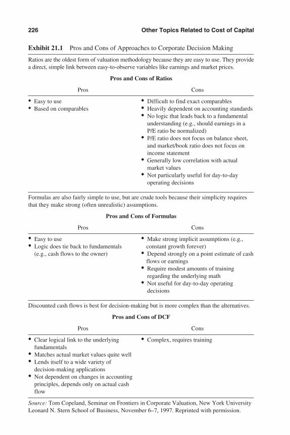
226 Other Topics Related to Cost of Capital
Exhibit 21.1 Pros and Cons of Approaches to Corporate Decision Making
Ratios are the oldest form of valuation methodology because they are easy to use. They providea direct, simple link between easy-to-observe variables like earnings and market prices.
Pros and Cons of Ratios
Pros Cons
• Easy to use • Difficult to find exact comparables• Based on comparables • Heavily dependent on accounting standards
• No logic that leads back to a fundamentalunderstanding (e.g., should earnings in aP/E ratio be normalized)
• P/E ratio does not focus on balance sheet,and market/book ratio does not focus onincome statement
• Generally low correlation with actualmarket values
• Not particularly useful for day-to-dayoperating decisions
Formulas are also fairly simple to use, but are crude tools because their simplicity requiresthat they make strong (often unrealistic) assumptions.
Pros and Cons of Formulas
Pros Cons
• Easy to use • Make strong implicit assumptions (e.g., • Logic does tie back to fundamentals constant growth forever)
(e.g., cash flows to the owner) • Depend strongly on a point estimate of cash flows or earnings
• Require modest amounts of training regarding the underlying math
• Not useful for day-to-day operatingdecisions
Discounted cash flows is best for decision-making but is more complex than the alternatives.
Pros and Cons of DCF
Pros Cons
• Clear logical link to the underlying • Complex, requires trainingfundamentals
• Matches actual market values quite well• Lends itself to a wide variety of
decision-making applications• Not dependent on changes in accounting
principles, depends only on actual cash flow
Source: Tom Copeland, Seminar on Frontiers in Corporate Valuation, New York UniversityLeonard N. Stern School of Business, November 6–7, 1997. Reprinted with permission.
3953 P-21 8/29/02 2:27 PM Page 226
opportunities unique to the project, may cause the WACC for the project to differfrom the company’s overall WACC.
However, a variation on DCF analysis, dubbed adjusted present value (APV), ad-vocates taking DCF analysis for project selection in a different direction. Instead of anoverall project WACC, the APV approach estimates a base-case value by unbundlingthe components of value and analyzing each separately. APV starts with a base-casevalue, discounting all cash flows from the project as if they were financed by equity. Itthen adds or subtracts increments or decrements of value from all financing side effects.The list includes:
• Interest tax shields
• Cost of financial distress
• Subsidies
• Hedges
• Issue costs
• Other costs5
Timothy A. Leuhrman, author of “Using APV: A Better Tool for Valuing Oper-ations,” claims “the particular version of DCF that has been accepted as the standardover the past 20 years—using the weighted average cost of capital (WACC) as thediscount rate—is now obsolete. . . . Adjusted present value (APV) is especially ver-satile and reliable, and will replace WACC as the DCF methodology of choice amonggeneralists.”6
USE TARGET COST OF CAPITAL OVER LIFE OF PROJECT
In any case, while the consensus advocates focusing on the cost of capital of theproject rather than on the overall company cost of capital to the extent that they differ,the focus should encompass the life of the project rather than any temporary effects. Forexample, if the project requires an abnormal level of debt financing that would tem-porarily change the company’s capital structure, the WACC should reflect the com-pany’s target capital structure rather than the abnormal structure when the investmentinitially is made.
SUMMARY
This is a short chapter, because the essential principles of using cost of capital forcapital budgeting and project selection are essentially the same as for other applica-tions already discussed.
The general consensus is:
• Discounted cash flow is the best model for corporate finance decisions.
• Focus on net cash flow as the economic income variable of choice.
Capital Budgeting and Feasibility Studies 227
3953 P-21 8/29/02 2:27 PM Page 227
• Each project should be analyzed in light of its own cost of capital characteristics,rather than automatically using the company’s overall cost of capital.
• The cost of capital used should be the target cost of capital over the life of theproject.
• New variations of cost of capital applications are constantly being developed.
Notes
1. Richard A. Brealey and Stewart C. Myers, Principles of Corporate Finance, 6th ed.(Boston: Irwin McGraw-Hill, 2000), 222.
2. Ibid, 221.3. Tom Copeland, Seminar on Frontiers in Corporate Valuation, New York University,
Leonard N. Stern School of Business, November 6–7, 1997.4. Ibid.5. Timothy A. Luehrman, “Using APV: A Better Tool for Valuing Operations,” Harvard
Business Review (May–June 1997): 145.6. Ibid., 145–153.
228 Other Topics Related to Cost of Capital
3953 P-21 8/29/02 2:27 PM Page 228
229
Chapter 22
Central Role of Cost of Capital in Economic Value Added1
Joel M. Stern, G. Bennett Stewart, III, and Donald H. Chew, Jr.
EVA Financial Management SystemEVA and the Corporate Reward System
EVA Bonus Plan: Simulating OwnershipLeveraged Stock Options: Making Ownership Real
Summary
An economic value added (EVA)–based performance measurement systemmakes the cost of capital explicit. In its simplest form, EVA is net operating profitafter taxes less a charge for the capital employed to produce those profits. The capi-tal charge is the required, or minimum, rate of return necessary to compensate all thefirm’s investors, debt holders, and shareholders for the risk of the investment.
EVA is charged for capital at a rate that compensates investors for bearing thefirm’s explicit business risk. The assessment of business risk is based on the Capi-tal Asset Pricing Model (CAPM), which allows for a specific, market-based evalu-ation of risk for a company and its individual business units using the concept of“beta.” In addition, the tax benefit of debt financing is factored into the cost of cap-ital, but in such a way as to avoid the distortions that arise from mixing operatingand financing decisions. To compute EVA, the operating profit for the company andfor each of the units is charged for capital at a rate that blends the after-tax cost ofdebt and equity in the target proportions each would plan to employ rather than theactual mix each actually uses year-by-year. Moreover, operating leases are capital-ized and considered a form of debt capital for this purpose. As a result, new investmentopportunities are neither penalized nor subsidized by the specific forms of financingemployed.
To illustrate, a company with a 10% cost of capital that earns a 20% return on$100 million of net operating assets has an EVA of $10 million. This says the com-pany is earning $10 million more in profit than is required to cover all costs, includ-ing the opportunity cost of tying up scarce capital on the balance sheet. In this sense,
3953 P-22 8/29/02 2:27 PM Page 229
EVA combines operating efficiency and balance sheet management into one measurethat can be understood by operating people.
For operating heads and top management alike, EVA holds out three principalways of increasing shareholder value:
1. Increase the return derived from the assets already tied up in the business. Runthe income statement more efficiently without investing any more capital on thebalance sheet.
2. Invest additional capital and aggressively build the business so long as the returnearned exceeds the cost of that new capital. (Targets based on rates of return suchas return on earnings (ROE) or return on investment (ROI), incidentally, can ac-tually discourage this objective when divisions are earning well above their costof capital, because taking on some EVA-increasing projects will lower their av-erage return.)
3. Stop investing in, and find ways to release capital from, activities that earn sub-standard returns. This means everything from turning working capital faster andspeeding up cycle times to consolidating operations and selling assets worthmore to others.
Besides making the cost of capital explicit, the EVA performance measure alsocan be designed to encourage tax-minimizing accounting choices and to incorporatea number of other adjustments intended to eliminate distortions of economic perfor-mance introduced by conventional accounting measures like earnings or ROE. Forexample, one notable shortcoming of GAAP (generally accepted accounting princi-ples) accounting stems from its insistence that many corporate outlays with longer-term payoffs (like research and development [R&D] or training) be fully expensedrather than capitalized and amortized over an appropriate period. While well suitedto creditors’ concerns about liquidation values, such accounting conservatism canmake financial statements unreliable as guides to going-concern values. More im-portant, to the extent GAAP’s conservatism is built into a company’s performancemeasurement and compensation system, it can unduly shorten managers’ planninghorizon.
In setting up EVA systems, we sometimes advise companies to capitalize por-tions of their R&D, marketing, training, and even restructuring costs. In cases ofother “strategic” investments with deferred payoffs, we have also developed a pro-cedure for keeping such capital “off the books” (for internal evaluation purposes) andthen gradually readmitting it into the manager’s internal capital account to reflect theexpected payoffs over time. As these examples are meant to suggest, EVA can beused to encourage a more farsighted corporate investment policy than traditional fi-nancial measures based upon GAAP accounting principles.
In defining and refining its EVA measure, Stern Stewart & Co. has identifiedover 120 shortcomings in conventional GAAP accounting. In addition to GAAP’s in-ability to handle R&D and other corporate investments, we have addressed perfor-mance measurement problems associated with standard accounting treatments of:
230 Other Topics Related to Cost of Capital
3953 P-22 8/29/02 2:27 PM Page 230
• Inventory costing and valuation
• Depreciation
• Revenue recognition
• The writing-off of bad debts
• Mandated investments in safety and environmental compliance
• Pension and postretirement medical expense
• Valuation of contingent liabilities and hedges
• Transfer pricing and overhead allocations
• Captive finance and insurance companies
• Joint ventures and start-ups
• Special issues of taxation, inflation, and currency translation
For most of these accounting issues, we have crafted a series of cases to illustrate theperformance measurement problem and devised a variety of practical methods tomodify reported accounting results in order to improve the accuracy with which EVAmeasures real economic income.
Of course, no one company is likely to trigger all 120 measurement issues. Inmost cases, we find it necessary to address only some 15 to 25 key issues in detail—and as few as five or 10 key adjustments actually are made in practice. We recom-mend that adjustments to the definition of EVA be made only in those cases that passfour tests:
1. Is it likely to have a material impact on EVA?
2. Can the managers influence the outcome?
3. Can the operating people readily grasp it?
4. Is the required information relatively easy to track or derive?
For any one company, then, the definition of EVA that is implemented ishighly customized with the aim of striking a practical balance between simplicityand precision.
To make the measure more user-friendly, we have also developed a managementtool called “EVA Drivers” that enables management to trace EVA through the incomestatement and balance sheet to key operating and strategic levers available to them inmanaging their business. This framework has proven to be quite useful in focusingmanagement’s attention, diagnosing performance problems, benchmarking with peers,and enhancing planning. More generally, it has helped people up and down the lineto appreciate the role they have to play in improving value. It also can help guardagainst an excessive preoccupation with improving individual operational metrics tothe detriment of overall performance. For example, a drive to increase productivity—or, say, a single-minded obsession with winning the Malcolm Baldrige Award—couldlead to unwarranted capital spending or to shifts in product mix that result in less EVA
Central Role of Cost of Capital in Economic Value Added 231
3953 P-22 8/29/02 2:27 PM Page 231
and value, not more. In the end, management must be held accountable for deliveringvalue, not improving metrics.2
EVA FINANCIAL MANAGEMENT SYSTEM
The real success of business today depends not on having a well-thought-out,far-reaching strategy but rather on reengineering a company’s business systems to re-spond more effectively to the new business environment of continuous change. Ourcontention at Stern Stewart is that just as this information revolution has created aneed for business process reengineering, it also has precipitated a need to reengineerthe corporate financial management system.
What do we mean by a financial management system? A financial managementsystem consists of all those financial policies, procedures, methods, and measuresthat guide a company’s operations and its strategy. It has to do with how companiesaddress such questions as:
• What are our overall corporate financial goals and how do we communicate them,both within the company and to the investment community?
• How do we evaluate business plans when they come up for review?
• How do we allocate resources—everything from the purchase of an individualpiece of equipment, to the acquisition of an entire company, to opportunities fordownsizing and restructuring?
• How do we evaluate ongoing operating performance?
• Last but not least, how do we pay our people, what is our corporate reward system?
Many companies these days have ended up with a needlessly complicated and,in many respects, hopelessly obsolete financial management system. For example,most companies use discounted cash flow analysis for capital budgeting evaluations.But when it comes to other purposes, such as setting goals and communicating withinvestors, the same companies tend to reach for accounting proxies—measures likeearnings, earnings per share (EPS), EPS growth, profit margins, ROE, and the like.To the extent this is true, it means there is already a “disconnect” between the cashflow–based capital budget and accounting-based corporate goals. To make mattersworse, the bonuses for operating people tend to be structured around achieving someannually negotiated profit figure.
This widespread corporate practice of using different financial measures for dif-ferent corporate functions creates inconsistency, and thus considerable confusion, inthe management process. And, given all the different, often conflicting, measures ofperformance, it is understandable that corporate operating people tend to throw uptheir hands and say, “So, what are you really trying to get me to do here? What is thereal financial mission of our company?”
With EVA, all principal facets of the financial management process are tied tojust one measure, making the overall system far easier to administer and understand.
232 Other Topics Related to Cost of Capital
3953 P-22 8/29/02 2:27 PM Page 232
That is, although the process of coming up with the right definition of EVA for anygiven firm is often complicated and time-consuming, the measure itself, once estab-lished, becomes the focal point of a simpler, more integrated overall financial man-agement system—one that can serve to unite all the varied interests and functionswithin a corporation.
Why is it so important to have only one measure? As we noted earlier, the nat-ural inclination of operating managers in large public companies is to get their handson more capital to spend and grow the empire. This tendency in turn leads to anovertly political internal competition for capital—one in which different performancemeasures are used to gain approval for pet projects. And because of this tendencytoward empire-building, top management typically feels compelled to interveneexcessively—not in day-to-day decision making but in capital spending decisions.Why? Because they do not trust the financial management system to guide their op-erating managers to make the right decisions. There is no real accountability built intothe system, and there is no real incentive for operating heads to choose only those in-vestment projects that will increase value.
EVA is the internal measure that management can decentralize throughout thecompany and use as the basis for a completely integrated financial management system.It allows all key management decisions to be clearly modeled, monitored, commu-nicated, and rewarded according to how much value they add to shareholders’ in-vestment. Whether reviewing a capital budgeting project, valuing an acquisition,considering strategic plan alternatives, assessing performance, or determining bonuses,the goal of increasing EVA over time offers a clear financial mission for managementand a means of improving accountability and incentives. In this sense, it offers a newmodel of internal corporate governance.
EVA AND THE CORPORATE REWARD SYSTEM
Incentive compensation is the anchor of the EVA financial management system.The term “incentive compensation” is not quite right, however, for in practice toomuch emphasis gets placed on the word “compensation” and not enough on the word“incentive.” The proper objective is to make managers behave as if they were owners.Owners manage with a sense of urgency in the short term but pursue a vision for thelong term. They welcome change rather than resisting it. Above all else, they person-ally identify with the successes and the failures of the enterprise.
Extending an ownership interest is also the best way to motivate managers in theinformation age. As the pace of change increases and the world becomes ever less pre-dictable, line managers need more general as opposed to specific measures of perfor-mance to which they will be held accountable. They need more leeway to respond tochanges in the environment. They need a broader and longer-range mandate to moti-vate and guide them. Maximizing shareholder value is the one goal that remains con-stant, even as the specific means to achieve it are subject to dramatic and unpredictableshifts.
Central Role of Cost of Capital in Economic Value Added 233
3953 P-22 8/29/02 2:27 PM Page 233
Making managers into owners should not be undertaken as an “add-on” to cur-rent incentive compensation methods. Rather, it should replace them. In place of thetraditional short-term bonus linked to budget and ordinary stock option grants, theEVA ownership plan employs two simple, distinct elements:
1. A cash bonus plan that simulates ownership
2. A leveraged stock option (LSO) plan that makes ownership real
EVA Bonus Plan: Simulating Ownership
The cash bonus plan simulates ownership primarily by tying bonuses to im-provements in EVA over time. Paying for improvements in, rather than absolute lev-els of, EVA is designed mainly to solve the problem of “unequal endowments.” Thisway managers of businesses with sharply negative EVA can be given a strong in-centive to engineer a turnaround—and those managers of businesses already produc-ing large positive EVA do not receive a windfall simply for showing up.
Besides leveling the playing field for managers inheriting different circum-stances, bonuses tied to improvements in rather than levels of EVA are also “self-financing” in the following sense: To the extent that a company’s current stock tendsto reflect current levels of EVA, it is only changes in current levels of EVA that arelikely to be correlated with changes in stock price.3 And, to the extent the managersof a given company succeed in increasing a company’s EVA and so earn higherbonus awards for themselves, those higher bonuses are more than paid for by the in-crease in shareholder value that tends to accompany increases in EVA.
As with a true ownership stake, EVA bonuses are not capped. They are poten-tially unlimited (on the downside as well as upside), depending entirely on manage-rial performance. But, to guard against the possibility of short-term “gaming” of thesystem, we have devised a “bonus bank” concept that works in this way: Annualbonus awards are not paid out in full but instead are banked forward and held “atrisk,” with full payout contingent on continued successful performance. Each year’sbonus award is carried forward from the prior year and a fraction—for example,one-third—of that total is paid out, with the remainder banked into the next year.
Thus, in a good year, a manager is rewarded—much like a shareholder who re-ceives cash dividends and capital appreciation—with an increase in both the cashbonus paid out and in the bonus bank carried forward. But in a poor year—again,much like a shareholder—the penalty is a shrunken cash distribution and a depletionin the bank balance that must be recouped before a full cash bonus distribution isagain possible. Because the bonus paid in any one year is an accumulation of thebonuses earned over time, the distinction between a long-term and a short-term bonusplan becomes meaningless.
When combined with such a bonus bank system, EVA incentive plans tied to con-tinuous improvement also help to break the counterproductive link between bonusesand budgets. EVA targets are automatically reset from one year to the next by formula,not annual negotiation. For example, if EVA should decline for whatever reason, man-
234 Other Topics Related to Cost of Capital
3953 P-22 8/29/02 2:27 PM Page 234
agement will suffer a reduced, possibly negative bonus in that year. In the followingyear, however, the minimal standard of performance for the next year’s bonus will beset somewhat lower—again, by a preset formula. This automatic lowering of expec-tations is designed to help companies retain and motivate good managers throughbad times by giving them a renewed opportunity to earn a decent bonus if they can re-verse the company’s fortune. At the same time, however, it avoids the problem—inherent in the stock option “repricing” practices of so many public companies—ofrewarding managers handsomely when the stock drops sharply and then simply re-turns to current levels.
In combination with a bonus bank, then, the use of objective formulas to resettargets eliminates the problems of “sandbagging” on budgets and encourages collab-orative, long-range planning. Instead of wasting time managing the expectations oftheir supervisors, managers are motivated to propose and execute aggressive businessplans. Moreover, because it compensates the end of creating value rather than themeans of getting there, the EVA bonus plan is entirely consistent with the movementto decentralize and empower.
In sum, the banking of bonuses tied to continuous improvements in EVA helpscompanies to smooth cyclical bumps and grinds, extends managers’ time horizons,and encourages good performers accumulating equity in their bank accounts to stayand poor performers running up deficits to go. In so doing, the EVA bonus bank func-tions as both a long-term and short-term plan at one and the same time.
Leveraged Stock Options: Making Ownership Real
The annual EVA cash bonus is intended to simulate an owner’s stake. In manycases, however, it is often valuable to supplement the bonus plan with actual stockownership by management. Pursuit of that goal, however, runs headlong into thisfundamental contradiction: How can managers with limited financial resources bemade into significant owners without unfairly diluting the current shareholders?Showering them with stock options of restricted stock is apt to be quite expensive forthe shareholders, notwithstanding the incentive for the managers. And asking themanagers to buy lots of stock is apt to be excessively risky for them.
One approach we recommend to resolve this dilemma is to encourage (or require)managers to purchase common equity in the form of special leveraged stock options(LSOs). Unlike ordinary options, these are initially in-the-money and not at-the-money,are bought and not granted, and project the exercise price to rise at a rate that sets asidea minimal acceptable return for the shareholders before management participates.
Although managers’ purchase of LSOs could be funded by them as a one-timeinvestment, we typically recommend that managers be allowed to buy them only witha portion of their EVA bonuses. Besides providing even more deferred compensation,this practice helps ensure that only those managers who have added value in theirown operations are allowed to participate in the success of the entire enterprise.
To illustrate how an LSO operates, consider a company with a current commonshare price of $10. The initial exercise price on the LSO is set at a 10% discount from
Central Role of Cost of Capital in Economic Value Added 235
3953 P-22 8/29/02 2:27 PM Page 235
the current stock price, or $9, making the option worth $1 right out of the gate. Butinstead of just handing the LSOs to management, managers are required to purchasethem for the $1 discount, and that money is put at risk. Another difference betweenLSOs and regular options is that the exercise price is projected to increase at a ratethat approximates the cost of capital (less a discount for undiversifiable risk andilliquidity)—let’s say 10% per annum. In this case, over a five-year period (and ig-noring compounding for simplicity), the exercise price will rise 50% above the cur-rent $9 level to $13.50. In sum, management pays $1 today for an option to purchasethe company’s stock (currently worth $10) for $13.50 five years down the road.
Only if the company’s equity value grows at a rate faster than the exercise pricewill management come out ahead. Indeed, if the exercise price rises at a rate equal tothe cost of capital (less the dividend yield), then the LSOs will provide exactly the sameincentives as an EVA bonus plan. It rewards management for generating a spread be-tween the company’s rate of return on capital and the cost of that capital (as reflectedby the rate of increase in the exercise price) times the capital employed by managementto purchase the shares.
Perhaps a better comparison, however, is between the incentives held out byLSOs and those provided by leveraged buyouts. LSOs can be seen as putting man-agement in the position of participating in an LBO, but without requiring an actualLBO of the company. By virtue of their being purchased 10% in the money, LSOs ef-fectively replicate the 90% debt and 10% equity that characterized the structure of theLBOs of the 1990s.
At bottom, then, LSOs (and LBOs, as we have seen) also boil down to EVA, tothe idea that management should participate only in those returns in excess of a com-pany’s required rate of return. But while conceptually identical to an EVA bonus plan,LSOs are likely to be an even more powerful motivator because they amplify the risksand rewards for management. Any improvement in EVA that investors think will besustained is capitalized into the value of the shares; for example, a company with acost of capital of 10% that increases its EVA by $1 million will see its value appre-ciate by $10 million. For managers holding the LSOs, such capitalized increases invalue are themselves further leveraged 10 to 1, thus creating $100 of added manage-rial wealth for each $1 improvement in EVA. This leveraging effect makes LSOs apotent way to get management to concentrate on building EVA over the long haul.
In sum, the EVA ownership plan replaces the traditional short-term bonus linkedto budget and ordinary stock option grants with two components:
1. A cash bonus plan that simulates ownership
2. A leveraged stock option plan that confers actual ownership
The cash bonus plan simulates ownership by tying bonuses to sustained improvementsin EVA over time, with a large portion of awarded bonuses held in escrow and sub-ject to loss to ensure that improvements are permanent. The LSO plan corrects the de-ficiencies of normal stock option plans in two ways:
236 Other Topics Related to Cost of Capital
3953 P-22 8/29/02 2:27 PM Page 236
1. The leverage factor allows managers to purchase significantly more stock for agiven amount of dollars (thus replicating an LBO’s effect on ownership)
2. A steadily rising exercise price ensures that managers win only if shareholders do
SUMMARY
An EVA financial management system represents a way to institutionalize therunning of a business in accordance with basic microeconomic and corporate financeprinciples. When properly implemented, it is a closed-loop system of decision mak-ing, accountability, and incentives—one that has the potential to make the entire or-ganization and not just the chief executive officer responsible for the successes andfailures of the enterprise. It can result in a self-regulated and self-motivated systemof “internal” governance.
As a concept, EVA starts simple, but in practice it can be made as comprehen-sive as necessary to accommodate management’s needs and preferences. EVA is mosteffective, however, when it is more than just a performance measure. At its best, EVAserves as the centerpiece of a completely integrated framework of financial manage-ment and incentive compensation.
The anchor of the EVA financial management system is a powerful incentivecompensation plan that consists of two parts:
1. A cash bonus plan tied to continuous improvement in EVA, in which a signifi-cant portion of the awarded bonuses is carried forward in a “bonus bank” andheld at risk
2. A leveraged stock option plan, in which managers use part of their cash bonusawards to make highly leveraged purchases of company stock
Such an EVA reward system holds out major benefits over more conventionalcompensation plans:
• Rewarding managers for continuous improvement in (rather than levels of) EVAmeans that new managers neither receive windfalls for inheriting already prof-itable divisions, nor are they penalized for stepping into turnaround situations.
• In contrast to compensation plans that continually revise performance criteria toprovide “competitive” compensation levels each year, the EVA bonus plan has a“long-term memory” in the form of a bonus bank that ensures that only consistent,sustainable increases in value are rewarded.
• EVA bonuses are tied to a performance measure that is highly correlated withshareholder value, thus aligning managers’ with shareholders’ interests.
• The strength of the correlation between changes in EVA and in shareholder valuealso means that the EVA compensation system is effectively “self-financing”;
Central Role of Cost of Capital in Economic Value Added 237
3953 P-22 8/29/02 2:27 PM Page 237
that is, managers win big only when shareholders are winning—and managers aretruly penalized when shareholders lose.
Proper internal governance is certainly no guarantee of success, and it is no sub-stitute for leadership, entrepreneurism, and hustle. But an EVA financial managementand incentive system can help. We like to say that EVA works like the proverbial Tro-jan horse: What is wheeled in appears to be an innocuous new financial managementand incentive program, but what jumps out is a new culture that is right for times ofrapid change and decentralized decision making. By increasing accountability,strengthening incentives, facilitating decentralized decision making, establishing acommon language and integrated framework, and fostering a culture that prizes build-ing value above all else, it significantly improves the chances of winning. That’s allany shareholder can reasonably expect from governance in today’s business environ-ment of continuous change.
Notes
1. This chapter is adapted with permission from a portion of “The EVA® Financial Man-agement System,” Journal of Applied Corporate Finance (summer 1995): 32–36.
2. Nevertheless, our research suggests a remarkably strong correlation between a company’sEVA performance, its shareholder value added (or MVA), and its standing in Fortune’sMost Admired survey, a ranking based on an assessment of such criteria as customer re-sponsiveness, innovation, time-to-market, and management quality. See Bennett Stewart,“EVA: Fact and Fantasy,” Journal of Applied Corporate Finance, Vol. 7, No. 2 (summer1994).
3. Our own research indicates that the changes in companies’ EVAs over a five-year periodaccount for nearly 50% of the changes in their market value added (MVAs), over that sametime frame. (MVA, which is a measure of the shareholder value added by management, isroughly equal to the difference between the total market value and the book value of thefirm’s equity.) By comparison, growth in sales explained just 10% of the MVA changes,growth in earnings per share about 15% to 20%, and return on equity only 35%. For a de-scription of this research, see Bennett Stewart, “Announcing the Stern Stewart Perfor-mance 1,000,” Journal of Applied Corporate Finance, Vol. 3 No. 2 (summer 1990).
238 Other Topics Related to Cost of Capital
3953 P-22 8/29/02 2:27 PM Page 238

Appendixes
3953 P-23 8/29/02 2:28 PM Page 239

3953 P-23 8/29/02 2:28 PM Page 240
241
Appendix A
Bibliography
This bibliography is separated into two sections—books and articles. AppendixB references relevant courses and conferences, and Appendix C lists data resourcesfor information on cost of capital.
BOOKS
Abrams, Jay B. Quantitative Business Valuation—A Mathematical Approach for Today’sProfessionals. New York: McGraw-Hill, 2001.
Adams, David P., et al. Fundamentals of Business Valuation—Part I. Lewisville, TX:American Institute of Certified Public Accountants, 2001.
ASA Business Valuation Standards and Portions of Uniform Standards of Professional Ap-praisal Practice. Herndon, VA: American Society of Appraisers, revised 1994.
Bierman, Harold, Jr., and Seymour Smidt. The Capital Budgeting Decision: EconomicAnalysis of Investment Projects, 8th ed. New York: Macmillan, 1992.
Brealey, Richard A., and Stewart C. Myers. Principles of Corporate Finance, 6th ed.Boston: Irwin McGraw-Hill, 2000.
Brown, Lawrence D., ed. I/B/E/S Research Bibliography, 5th ed. New York: I/B/E/S In-ternational, Inc., 1996.
Copeland, Tom, Tim Koller, and Jack Murrin. Valuation: Measuring and Managing theValue of Companies, 3rd ed. New York: John Wiley & Sons, Inc., 2000.
Cornell, Bradford. Corporate Valuation: Tools for Effective Appraisal and Decision Mak-ing. New York: McGraw-Hill, 1993.
———. The Equity Risk Premium: The Long-Run Future of the Stock Market. New York:John Wiley & Sons, Inc., 1999.
Damodaran, Aswath. Damodaran on Valuation: Security Analysis for Investment andCorporate Finance. New York: John Wiley & Sons, Inc., 1994.
———. Investment Valuation, 2nd ed. New York: John Wiley & Sons, Inc., 2002.
Ehrhardt, Michael C. The Search for Value: Measuring the Company’s Cost of Capital.Boston: Harvard Business School Press, 1994.
Friend, Irwin I., and I. Bisksler, eds. Risk and Return in Finance. Cambridge, MA:Ballinger, 1977.
3953 P-23 8/29/02 2:28 PM Page 241
Fishman, Jay E., Shannon P. Pratt, J. Clifford Griffith, and Mark Wells. Guide to Busi-ness Valuations, 11th ed. Fort Worth, TX: Practitioners Publishing Co., 2001 (updatedannually).
Hitchner, James R., Financial Valuation: Applications and Models. New York: JohnWiley & Sons, Inc., forthcoming.
Hull, J. Options, Futures and Other Derivative Securities. Englewood Cliffs, NJ: Prentice-Hall, 1993.
Ibbotson Associates. Beta Book, First 2001 ed. Chicago: Ibbotson Associates, 2001.
———. Cost of Capital Workshop. Chicago: Ibbotson Associates, 1998.
———. Cost of Capital Yearbook. Chicago: Ibbotson Associates, 2002.
———. Stocks, Bonds, Bills and Inflation Classic Edition 2002 Yearbook. Chicago: Ib-botson Associates, 2002.
Ibbotson, Roger G., and Gary P. Brinson. Global Investing: The Professional’s Guide tothe World Capital Markets. New York: McGraw-Hill, 1993.
Ibbotson, Roger G., and Gary P. Brinson. Investment Markets. New York: McGraw-Hill,1987.
IRS Training for Appeals Officers Coursebook. Chicago: CCH Incorporated, 1998.
Kaufman, Mike. Handbook of Budgeting, 4th ed. New York: John Wiley & Sons, Inc.,1999.
Mercer, Z. Christopher, Quantifying Marketability Discounts—Developing and Support-ing Marketability Discounts in the Appraisal of Closely Held Business Interests,Memphis, TN: Peabody Publishing, LP, 1997.
———. Valuing Financial Institutions. Homewood, IL: Business One Irwin, 1992.
Pratt, Shannon P. Business Valuation Discounts and Premiums. New York: John Wiley& Sons, Inc., 2001.
Pratt, Shannon P., Robert F. Reilly, and Robert P. Schweihs. Valuing a Business: TheAnalysis and Appraisal of Closely Held Companies, 4th ed. New York: McGraw-Hill,2000.
———. Valuing Small Businesses and Professional Practices, 3d ed. New York: Mc-Graw-Hill, 1998.
Rachlin, Robert, and H. W. Allend Sweeny. Handbook of Budgeting, 3d ed. New York:John Wiley & Sons, Inc., 1993. See especially Chapter 11, “Determining the Cost ofCapital,” by Mike Kaufman.
Rapport, Alfred. Creating Shareholder Value, revised ed. New York: The Free Press,1998.
Reilly, Frank K. Investment Analysis and Portfolio Management, 4th ed. Forth Worth,TX: Dryden Press, 1994.
Ross, Stephen A., Randolph W. Westerfield, and Jeffrey F. Jaffe. Corporate Finance, 4thed. Burr Ridge, IL: McGraw-Hill, 1996.
Sharpe, William F., G. J. Alexander, and J.V. Bailey. Investments, 6th ed. EnglewoodCliffs, NJ: Prentice-Hall, 1998.
Standard & Poor’s Corporate Value Consulting. Risk Premium Report (formerly thePricewaterhouseCoopers Risk Premium Study).
242 Appendix A
3953 P-23 8/29/02 2:28 PM Page 242
Williams, John Burr. The Theory of Investment Value. Cambridge, MA: Harvard Univer-sity Press, 1938.
ARTICLES
Abrams, Jay B. “A Breakthrough in Calculating Reliable Discount Rates.” ASA Valuation(August 1994): 8–24.
———. “The Right Tools Can Simplify Company Valuation.” Accounting Today (No-vember 6, 1995): 14, 35.
Annin, Michael. “Fama-French and Small Company Cost of Equity Calculations.” Busi-ness Valuation Review (March 1997): 3–13.
———. “Using Ibbotson Associates’ Data to Develop Minority Discount Rates.” CPAExpert (Winter 1997): 1–4.
Annin, Michael E., and Dominic A. Falaschetti. “Equity Risk Premium Still Produces De-bate.” Valuation Strategies (January/February 1998): 17–23, 44.
———. “Is There Still a Size Premium?” CPA Expert (Winter 1998): 7–9.
Ashton, D. J. “The Cost of Equity Capital and a Generalization of the Dividend GrowthModel.” Accounting & Business Research (Winter 1995): 3–17.
Asness, Clifford S. “Stocks versus Bonds: Explaining the Equity Risk Premium.” Finan-cial Analysts Journal (March/April 2000): 96–113.
“Bankruptcy Court Determines Fair Market Value Under Pennsylvania Judgment.”Judges & Lawyers Business Valuation Update (May 2000): 7.
Baptiste, Laurent, Gregory Borges, and Gary Carr. “Utility Bond Ratings and the Cost ofCapital.” Public Utilities Fortnightly (October 27, 1988).
Barber, Gregory A. “Valuation of Pass-Through Entities.” Valuation Strategies(March/April 2001): 4–11, 44.
Becker, Brian C., and Ian Gray. “Does a Small Firm Effect Exist When Using the CAPM?Not Since 1980 and Not When Using Geometric Means of Historical Returns.” Busi-ness Valuation Review (September 1999): 104–107.
———. “Using Average Historical Data for Risk Premium Estimates: Arithmetic Mean,Geometric Mean, or Something Else?” Business Valuation Review (December 1998):136–140.
Bendixen, Christian L. “Improved Estimation of Equity Risk Premiums.” Business Valu-ation Review (March 1994): 22–32.
Berk, Jonathan B. “Does Size Really Matter?” Financial Analysts Journal(September–October 1997): 12–18.
Bishop, David M., and Frank C. Evans. “Avoiding a Common Error in Calculating theWeighted Average Cost of Capital.” CPA Expert (Fall 1997): 4–6.
Black, Fischer. “Estimating Experted Return.” Financial Analysts Journal (September–October 1993): 36–38.
Bishop, David M., and Frank C. Evans. “Avoiding a Common Error in Calculating theWeighted Average Cost of Capital.” CPA Expert (Fall 1997): 4–6.
Bibliography 243
3953 P-23 8/29/02 2:28 PM Page 243
Bishop, David M., and John P. White. “Overview of the Multiple Period DiscountingMethod: Practical Considerations for Application in the Valuation of Businesses.”American Society of Appraisers International Conference 2001. Pittsburgh, Pa. Avail-able at www.BVLibrary.com.
Bolton, Steven, and Yan Wang. “The Impact of Management Depth on Valuation.” Busi-ness Valuation Review (September 1997): 143–146.
Booth, Laurence. “The Capital Asset Pricing Model + Equity Risk Premiums and the Pri-vately-Held Business.” 1998 CICBV/ASA Joint Business Valuation Conference, Sep-tember 24–25, 1998, Montreal, Canada.
Booth, Laurence, and Cleveland S. Patterson. “Estimating the Cost of Equity Capital of aNon-Traded Unique Canadian Entity: Reply.” Canadian Journal of AdministrativeSciences (June 1993): 122–133.
Botosan, Christine A. “Disclosure Level and the Cost of Equity Capital.” Accounting Re-view (July 1997): 323–349.
Boudoukh, Jacob, Matthew Richardson, and Robert F. Whitelaw. “Nonlinearities in theRelation Between the Equity Risk Premium and the Term Structure.” Management Sci-ence (March 1997): 371–385.
Budyak, James T. “Getting a Grip on Foreign Discount Rates.” (January 2000). Availableat www.BVLibrary.com.
———. “Establishing Discount Rates in a Global Environment.” ASA International Ap-praisal Conference. Pittsburgh, Penn. July 2001.
Burmeister, Edwin, Richard Roll, and Stephen A. Ross. “A Practitioner’s Guide to Arbi-trage Pricing Theory.” In A Practitioner’s Guide to Factor Models. Charlottesville,VA: Research Foundation of the Institute of Chartered Financial Analysts, 1994.
Burns, Richard M. “Using DCF Analysis.” 1999 Institute of Business Appraisers NationalConference—Business Valuations. Orlando, Fla. Available at www.BVLibrary.com.
Carlton, Willard T., and Josef Lakonishok. “Risk and Return on Equity: The Use and Mis-use of Historical Estimates.” Financial Analysts Journal (January–February 1985):38–47.
Cassiere, George G. “Geometric Mean Return Premium Versus the Arithmetic Mean Re-turn Premium—Expanding on the SBI 1995 Yearbook Examples.” Business ValuationReview (March 1996): 20–23.
Chen, Nai-fi, Richard Roll, and Stephen A. Ross. “Economic Forces and the Stock Mar-ket: Testing the APT and Alternative Asset Pricing Theories.” UCLA Graduate Schoolof Management Working Paper No. 20-83 (December 1983).
Clineball, John M., Douglas R. Kahl, and Jerry L. Stevens. “Time-Series Properties of theEquity Risk Premium.” Journal of Financial Research (Spring 1994): 105–116.
Clubb, Colin D. B., and Paul Doran. “On the Weighted Average Cost of Capital with Per-sonal Taxes.” Accounting & Business Research (Winter 1992): 44–48.
Copeland, Tom. Seminar on Frontiers in Corporate Valuation. New York UniversityLeonard N. Stern School of Business (November 6–7, 1997).
Cornell, Bradford. “Estimating the Cost of Equity Capital.” Proceedings of the 27th An-nual Wichita Program: Appraisal for Ad Valorem Taxation, August 3–7, 1997. Wi-chita, KS: Wichita State University, 1997.
244 Appendix A
3953 P-23 8/29/02 2:28 PM Page 244
Cummins, J. David, and Joan Lamm-Tennant. “Capital Structure and the Cost of EquityCapital in the Property-Liability Insurance Industry.” Insurance: Mathematics & Eco-nomics (December 1994): 187–201.
Damodaran, Aswath. “Estimating Equity Risk Premiums.” Stern School of BusinessWorking Paper No. FIN-99-021, 1999. Can be downloaded without charge athttp://www.stern.nyu.edu/fin.
Dempsey, Mike. “The Cost of Equity Capital at the Corporate and Investor Levels: Al-lowing a Rational Expectations Model with Personal Taxations.” Journal of BusinessFinance & Accounting (December 1996): 1319–1331.
Dickerson, Gregg. “Estimating the Cost of Equity or They Ripped Out My CAPM andStomped That Sucker Flat.” Proceedings of the 27th Annual Wichita Program: Ap-praisal for Ad Valorem Taxation, August 3–7, 1997, Wichita, Kansas.
Dietrich, Mark O. “Tax Effecting Nontaxable Entities’ Earnings Post-Gross.” July 10,2000. Available at www.cpa.net/postgross.html.
Dilbeck, Harold R. “A Constant-Dollar Discount Rate for Closely Held Businesses Basedon Risk Premiums from Five-Year Holding Periods.” Business Valuation Review(March 1994): 11–18.
Dobner, Michael. “Mid Year Discounting and Seasonality Factors.” Business ValuationReview (March 2002): 16–18.
Downs, Thomas W., and Robert W. Ingram. “Beta, Size, Risk, and Return.” Journal ofFinancial Research (Fall 2000): 245–260.
Durand, David. “Afterthoughts on a Controversy with MM, Plus New Thoughts onGrowth and the Cost of Capital.” Financial Management (Summer 1989): 12–18.
Duvall, Richard M. “Mid-year or End-of-year Discounting.” Business Valuation Review(December 2000): 208–211.
———. “Capitalization of Earnings with Temporary Rapid Growth.” Business ValuationReview (June 2001): 3–4.
Eccles, Robert G., Kersten L. Lanes, and Thomas C. Wilson. “Are You Paying Too Muchfor That Acquisition?” Harvard Business Review (July–August 1999): 136–146.
Evans, Frank C. “Practice Development/Business Valuation: Tips for the Valuator.” Jour-nal of Accountancy (March 2000): 5–42.
———. “Making Sense of Rates of Return and Multiples.” Business Valuation Review(June 1999): 51–57.
Evans, Frank C., and Kelly L. Strimbu. “Debt and Equity Weightings in WACC.” CPAExpert (Fall 1998): 4–5.
Fama, Eugene, and Kenneth French. “Common Risk Factors in the Returns on Stocksand Bonds.” University of Chicago Working Paper No. 360 (November 1992).
Fama, Eugene F., and Kenneth R. French. “Taxes, Financing Decisions, and Firm Value.”Journal of Finance (June 1998): 819–843.
———. “The Equity Premium.” The Journal of Finance (April 2002): 637–659.
Fowler, Bradley A. “How Do You Handle It?” part of a Special Report “ASA ConferenceOffers Valuable Insights.” Shannon Pratt’s Business Valuation Update (July 1997): 1–2.
Glazer, Jeffrey S. “The Capital Asset Pricing Model: Risk, Valuation, Judicial Interpre-tation and Market Bias.” 50 Bus. Law 686 (1995).
Bibliography 245
3953 P-23 8/29/02 2:28 PM Page 245
Goldenberg, David H., and Ashok J. Robin. “The Arbitrage Pricing Theory and Cost-of-Capital Estimation: The Case of Electric Utilities.” Journal of Financial Research(Fall 1991): 181–196.
———. “The Cross Section of Expected Stock Returns.” Journal of Finance 47 (1992):427–465.
Good, Walter R. “Yes, Virginia, There Is a Risk Premium, But . . .” Financial AnalystsJournal (January–February 1994): 11–12.
Grabowski, Roger, and David King. “New Evidence on Size Effects and Rates of Re-turn.” Business Valuation Review (September 1996): 103–115.
———. “Size Effects and Equity Returns, An Update.” Business Valuation Review(March 1997): 22–26.
———. “New Evidence on Equity Returns and Company Risk.” Business Valuation Re-view (September 1999): 112–130.
———. “New Evidence on Equity Returns and Company Risk: A Revision.” BusinessValuation Review (March 2000): 32.
Graham, John R. “Debt and the Marginal Tax Rate.” Journal of Financial Economics(1996): 41–73.
———. “Proxies for the Corporate Marginal Tax Rate.” Journal of Financial Economics(1996): 187–221.
Graham, John R., Michael L. Lemmon, and James S. Schallheim. “Debt, Leases, Taxes,and the Endogeneity of Corporate Tax Status.” Journal of Finance (February 1998):131–162.
Greer, Willis R. “The Growth Rate Term in the Capitalization Model.” Business Valua-tion Review (June 1996): 72–79.
Gullihur, James K. “The Gross Decision—Tax-effecting S Corporation Earnings.” Pitts-burgh, Pa. (October 2001). Available at www.BVLibrary.com.
Hanley, Frank J., and A. Gerald Harris. “Does Diversification Increase the Cost of EquityCapital?” Public Utilities Fortnightly (July 15, 1991): 26–30.
Hawkins, George B. “Valuation of S Corporations Using the Discounted Future IncomeMethod—A Tax Court Valuation Bombshell.” Fair Value (Fall 1999): 1–4.
———. “A Gross Result in the Gross Case Calls into Question Circumstances in WhichTax Affecting Is Valid.” Shannon Pratt’s Business Valuation Update (January 2002):5–7.
———. “Critically Assessing a Business Valuation: Is the Capitalization Rate Used Rea-sonable?” Fair Value (Spring 1996): 1–6.
Honnold, Keith L. “The Link Between Discount Rates and Capitalization Rates: Revis-ited.” Appraisal Journal (April 1990): 190–195.
Howton, Shelly W., and David R. Peterson. “A Cross-sectional Empirical Test of a Dual-state Multi-factor Pricing Model.” Financial Review (August 1999): 47–64.
Ibbotson, Roger G. “Equity Risk Premium: Where We Stand Today.” Proceedings of theEquity Risk Premium Conference, University of Chicago, June 6, 1996. Chicago: Ib-botson Associates, 1996.
Ibbotson, Roger G., and Peng Chen. “Stock Market Returns in the Long Run: Participat-ing in the Real Economy.” Yale ICF Working Paper No. 00-44, March 2002. Can bedownloaded without charge at http://papers.ssrn.com/abstract=274150.
246 Appendix A
3953 P-23 8/29/02 2:28 PM Page 246
Ibbotson, Roger G., Paul D. Kaplan, and James D. Peterson. “Estimates of Small-StockBetas Are Much Too Low.” Journal of Portfolio Management (Summer 1997).
Ickert, Donald W. “Unsystematic Risk & Size Effects on Valuation.” Presented at Amer-ican Society of Appraisers 2001 International Appraisal Conference, Pittsburgh, PA(July 23–25, 2001): Available at BVLibrary.com.
———. “Unsystematic Risk & Size Effects on Valuations.” (October 2001). Available atwww.BVLibrary.com.
Indro, Daniel C., and Wayne Y. Lee. “Biases in Arithmetic and Geometric Averages asEstimates of Long-run Expected Returns and Risk Premia.” Financial Management(Winter 1997): 81–90.
Johnson, Bruce A. “S Corporation Tax Treatment.” 2001 ASA International AppraisalConference. Available at www.BVLibrary.com.
Jackson, Marcus. “The Gordon Growth Model and the Income Approach to Value.” Ap-praisal Journal (January 1994): 124–128.
Joyce, Allyn A. “Arithmetic Mean vs. Geometric Mean: THE Issue in Rate of Return De-rivation.” Business Valuation Review (June 1995): 62–68.
———. “Why the Expected Rate of Return Is a Geometric Mean.” Business ValuationReview (March 1996): 17–19.
Julius, J. Michael. “Market Returns in Rolling Multi-Year Holding Periods: An Alterna-tive Interpretation of the Ibbotson Data.” Business Valuation Review (June 1996):57–71.
Kairys, Joseph P., Jr. “Predicting Sign Changes in the Equity Risk Premium Using Com-mercial Paper Rates.” Journal of Portfolio Management (Fall 1993): 41–51.
Kaltman, Todd A. “Capitalization Using a Mid-Year Convention.” Business ValuationReview (December 1995): 178–182.
Kaplan, Paul D. “Why the Expected Rate of Return Is an Arithmetic Mean.” BusinessValuation Review (September 1995): 126–129.
Kaplan, Paul D., and James D. Peterson. “Full-information Industry Betas.” FinancialManagement (Summer 1998): 85–93.
Kaplan, Steven J., and Richard S. Ruback. “The Valuation of Cash Flow Forecasts: AnEmpirical Analysis.” 50 Journal of Finance 1054, 1091 (1995).
Keck, Tom, Eric Levengood, and Al Longfield. “Using Discounted Cash Flow Analysisin an International Setting: A Survey of Issues in Modeling the Cost of Capital.” Jour-nal of Applied Corporate Finance (Fall 1998): 82–99.
Kenny, Thomas J. “Closely Held Corporation Valuation: Determining a Proper DiscountRate.” Business Valuation Review (March 1992): 22–30.
Kholdy, Shady, and Ahmad Sohrabian. “Internal Finance and Corporate Investment.” Fi-nancial Review (May 2001): 97–114.
Kihm, Steven G. “The Superiority of Spot Yields in Estimating Cost of Capital.” PublicUtilities Fortnightly (February 1, 1996): 42–45.
Kincheloe, Stephen C. “The Weighted Average Cost of Capital—The Correct DiscountRate.” Appraisal Journal (January 1990): 88–95.
King, David W. “The Equity Risk Premium for Cost of Capital Studies: Alternatives toIbbotson.” Business Valuation Review (September 1994): 123–129.
Bibliography 247
3953 P-23 8/29/02 2:28 PM Page 247
———. “Recent Evidence on Discount Rates.” Proceedings of the AICPA 1995 NationalBusiness Valuation Conference, New Orleans, LA, December 1995, pp. 12-i–12-13.Available on Business Valuation Update Online.
Krueger, Mark K., and Charles M. Linke. “A Spanning Approach for Estimating Divi-sional Cost of Capital.” Financial Management (Spring 1994): 64–70.
Lally, Martin. “The Accuracy of CAPM Proxies for Estimating a Firm’s Cost of Equity.”Accounting & Finance (May 1995): 63–72.
Lamdin, Douglas J. “New Estimates of the Equity Risk Premium and Why BusinessEconomists Need Them.” Department of Economics, University of Maryland, January2002.
Lavely, Joe, and Frank Bacon. “Risk and Rate of Return for Electric Utilities.” PublicUtilities Fortnightly (September 1, 1993): 18–20.
Leibowitz, Mark L., forum chair. “Equity Risk Premium Forum.” Association of Invest-ment Management and Research, November 8, 2001.
Leibowitz, Martin L., “Spread-driven Dividend Discount Models.” Financial AnalystsJournal (November/December 2000): 64–77.
Lerch, Mary Ann. “Pretax/Aftertax Conversion Formula for Capitalization Rates andCash Flow Discount Rates.” Business Valuation Review (March 1990): 18–22.
———. “Are We Capitalizing the Right Measure of Cash Flow?” Business Valuation Re-view (September 2001): 32–34.
Leuhrman, Timothy A. “Using APV: A Better Tool for Valuing Operations.” HarvardBusiness Review (May–June 1997): 145.
Levy, Moshe, and Haim Levy. “The Danger of Assuming Homogeneous Expectations.”Financial Analysts Journal (May–June 1996): 65–70.
Lippitt, Jeffrey W., and Nicholas J. Mastriacchio. “Developing Capitalization Rates forValuing a Business.” The CPA Journal (November 1995): 24–28.
Madden, Bartley J. “The CFROI Valuation Model.” Journal of Investing (Spring 1998):31–44.
Mandron, Alix. “DCF Valuation Can, and Should, Be Improved.” Montreal, Canada.Available at www.BVLibrary.com.
Mard, Michael J., and James S. Rigby. “New Research to Estimate Cost of Capital.” CPAExpert (Fall 1995): 9–12.
Maris, Brian A., and Fayez A. Elayan. “Capital Structure and the Cost of Capital for Un-taxed Firms: The Case of REITs.” Journal of the American Real Estate & Urban Eco-nomics Association (Spring 1990): 22–39.
Martin, Harold G., Jr., and Ronald L. Seigneur. “Cost of Capital.” Joint presentation madeat the American Institute of Certified Public Accountants National Business ValuationConference, Las Vegas, NV (December 4, 2001). Available at www.BVLibrary.com.
Mastriacchio, Nicholas J., and Jeffrey W. Lippitt. “A Comparison of the Earnings Capi-talization and the Excess Earnings Models in the Valuation of Closely Held Busi-nesses.” Journal of Small Business Management (January 1996): 1–12.
Matthews, Gilbert E. “Cap X = Depreciation Is Unrealistic Assumption for Most Termi-nal Values.” Shannon Pratt’s Business Valuation Update (March 2002): 1–3.
248 Appendix A
3953 P-23 8/29/02 2:28 PM Page 248
McConaughy, Daniel L. “Negative Takeover Premia and Stock Price Levels in InternetStocks.” Valuation Strategies (March–April 2002): 20–29.
Mercer, Z. Christopher. “The Adjusted Capital Asset Pricing Model for Developing Cap-italization Rates.” Business Valuation Review (December 1989): 147–156.
Meyer, James E., Patrick Fitzgerald, and Mostafa Moini. “Loss of Business Profits, Risk,and the Appropriate Discount Rate.” Journal of Legal Economics (Winter 1994):27–42.
Miller, Warren D. “Assessing Unsystematic Risk.” CPA Expert (Summer 1999): 1–5.
———. “Assessing Unsystematic Risk: Part II—The Macroenvironment.” CPA Expert(Winter 2000): 1–5.
Moyer, R. Charles, and Ajay Patel. “The Equity Market Risk Premium: A Critical Lookat Alternative Ex Ante Estimates.” Proceedings of the Ibbotson Equity Risk PremiumConference, University of Chicago, June 6, 1996. Chicago: Ibbotson Associates, 1996.Abstracted in Shannon Pratt’s Business Valuation Update (August 1996): 1–2.
“New Studies Quantifying Size Premiums Offer Strong Cost of Capital Support.” Shan-non Pratt’s Business Valuation Update (August 1997): 1, 3.
O’Brien, Thomas J. “The Global CAPM and a Firm’s Cost of Capital in Different Cur-rencies.” Journal of Applied Corporate Finance (Fall 1999): 73–79.
Olsen, Robert A., and George H. Troughton. “Are Risk Premium Anomalies Caused byAmbiguity?” Financial Analysts Journal (March/April 2000): 24–31.
Paolo, Stanley B. S. “The Weighted Average Cost of Capital: A Caveat.” EngineeringEconomist (Winter 1992): 178–183.
Paschall, Michael A., and George B. Hawkins. “Are Smaller Companies More Risky?”Fair Value (Fall 1999): 1, 5–12.
Pastor, Lubos, and Robert Stambaugh. “Cost of Equity Capital and Model Mispricing.”Journal of Finance (February 1999): 67–114.
Patterson, Cleveland S. “The Cost of Equity Capital of a Non-Traded Unique Entity: ACanadian Study.” Canadian Journal of Administrative Sciences (June 1993): 115–121.
Pratt, Shannon P. “Alternative Equity Risk Premium Measures Unstable; Lack Robust Pre-dictive Power.” Shannon Pratt’s Business Valuation Update (August 1996): 1–2.
———. “Building Better Betas Is Ibbotson’s Answer to Beta Controversy.” ShannonPratt’s Business Valuation Update (August 1997): 1–2.
———. “Discount Rates Based on CAPM Don’t Always Lead to Minority Value.” Shan-non Pratt’s Business Valuation Update (March 2001): 1–3.
———. “Evidence Suggests Equity Risk Premium Lower Than Conventional WisdomThinks.” Shannon Pratt’s Business Valuation Update (July 1996): 1–5.
———. “New Measures of Risk That Really Work.” Shannon Pratt’s Business ValuationUpdate (December 1999): 1–4.
———. “Practitioners Disagree Strongly on Excess Earnings Methodology.” ShannonPratt’s Business Valuation Update (April 1997): 1–3.
Raabe, William A., and Gerald E. Whittenburg. “Is the Capital Asset Pricing Model Ap-propriate in Tax Litigation?” Valuation Strategies (January/February 1998): 10–15,36–37.
Bibliography 249
3953 P-23 8/29/02 2:28 PM Page 249
Reynolds, Kevin B. “Reconciling the Single Period Capitalization Method with the Dis-counted Future Earnings Method.” Business Appraisal Practice (Spring 2000): 16–27.
Rigby, Jim, and Michael J. Mattson. “Capitalization and Discount Rates: MathematicallyRelated, but Conceptually Different.” CPA Expert (Fall 1996): 1–3.
Roll, Richard, and Stephen A. Ross. “On the Cross-sectional Relation between ExpectedReturns and Betas.” 49 Journal of Finance 101 (1994).
Ross, Stephen A. “The Arbitrage Theory of Capital Asset Pricing.” Journal of EconomicTheory (December 1976): 241–260.
Schramm, Ronald M., and Henry M. Wang. “Measuring the Cost of Capital in an Inter-national CAPM Framework.” Journal of Applied Corporate Finance (Fall 1999):63–72.
Scott, M. F. G. “The Cost of Equity Capital and the Risk Premium on Equities.” AppliedFinancial Economics (March 1992): 21–32.
Sharpe, William F. “Factor Models, CAPMs, and the ABT.” Journal of Portfolio Man-agement (Fall 1984): 21–25.
———. “Capital Asset Prices With and Without Negative Holdings.” Nobel Lecture, De-cember 1990. Stockholm: The Nobel Foundation, Royal Swedish Academy of Sci-ences, 1990.
Shumway, Tyler. “The Delisting Bias in CRSP Data.” Journal of Finance (March 1997).
Siegel, Jeremy, and Richard Thaler. “The Equity Risk Premium Puzzle.” Journal of Eco-nomic Perspectives, vol. 11, no. 1 (Winter): 191–200.
Sliwoski, Leonard. “Capitalization Rates Developed Using the Ibbotson Associates Data:Should They Be Applied to Pretax or After Tax Earnings?” Business Valuation Review(March 1994): 8–10.
Sliwoski, Leonard J. “Risk Categorization, the Income Approach, and the Invested Cap-ital Methodology (Part One).” Business Appraisal Practice (Winter 2000–2001):10–21.
———. “Risk Categorization, the Income Approach, and the Invested Capital Methodology(Part Two).” Business Appraisal Practice (Spring/Summer 2001): 43–53.
Stanton, Thomas C. “The Market Model: An Alternative to the CAPM.” Business Valu-ation Review (March 1999): 12–15. Available at www.BVLibrary.com.
———. “The Anatomy of Beta: Getting Down to Basics.” Business Appraisal Practice(Fall 1999): 34–38. Available at www.BVLibrary.com.
“Stock Recipients Liable for Fraudulent Transfer Underpayment.” Shannon Pratt’s Busi-ness Valuation Update (January 1999): 10.
Stultz, René M. “Globalization, Corporate Finance, and the Cost of Capital.” Journal ofApplied Corporate Finance (Fall 1999): 8–25.
Suvas, Arto. “Cost of Equity Capital Redefined.” Quarterly Journal of Business & Eco-nomics (Spring 1992): 53–71.
Swad, Randy. “Discount and Capitalization Rates in Business Valuations.” CPA Journal(October 1994): 40–46.
Tarbell, Jeffrey S. “The Small Company Risk Premium: Does It Really Exist?” AmericanSociety of Appraisers 18th Annual Advanced Business Valuation Conference. New Or-leans, La. October 29, 1999. Available at www.BVLibrary.com.
250 Appendix A
3953 P-23 8/29/02 2:28 PM Page 250
Thompson, Howard E., and Wing K. Wong. “On the Unavoidability of ‘Unscientific’Judgment in Estimating the Cost of Capital.” Managerial & Decision Economics (Feb-ruary 1991): 27–42.
Thompson, Samuel C., Jr. “A Lawyer’s Guide to Modern Valuation Techniques in Merg-ers and Acquisitions.” The Journal of Corporation Law (Spring 1996): 457–537.
———. “Demystifying the Use of Beta in the Determination of the Cost of Capital andan Illustration of Its Use in Lazard’s Valuation of Conrail.” The Journal of Corpora-tion Law (Winter 2000): 241–306.
Trout, Robert R. “Mid-year Discounting Without Bias.” Business Valuation Review (De-cember 2001): 39–41.
Vander Linden, Eric. “Cost of Capital Derived from Ibbotson Data Equals MinorityValue?” Business Valuation Review (December 1998): 123–127.
Vasicek, Oldrich A. “A Note on Using Cross-Sectional Information in Bayesian Estima-tion of Security Prices.” Journal of Finance (1973).
Welch, Ivo. “The Equity Premium Consensus Forecast Revisited.” Cowles Foundation forResearch in Economics at Yale University, Cowles Foundation Discussion Paper No.1325, September 2001. Can be downloaded without charge at http://papers.ssrn.com/abstract=285169.
Yamaguchi, Katsunari. “Estimating the Equity Risk Premium from Downside Probabil-ity.” Journal of Portfolio Management (Summer 1994): 17–27.
Young, David S. “Some Reflections on Accounting Adjustments and Economic ValueAdded.” Journal of Financial Statement Analysis (Winter 1999): 7–19.
Bibliography 251
3953 P-23 8/29/02 2:28 PM Page 251
252
Appendix B
Courses and ConferencesCourses by Professional Associations
American Society of AppraisersAmerican Institute of Certified Public AccountantsCenter for Advanced Valuation StudiesInstitute of Business AppraisersNational Association of Certified Valuation Analysts
Schedules and Other Conferences
COURSES BY PROFESSIONAL ASSOCIATIONS
The American Society of Appraisers (ASA), the American Institute of CertifiedPublic Accountants (AICPA), the Institute of Business Appraisers (IBA), and the Na-tional Association of Certified Valuation Analysts (NACVA) offer certain courses withsubstantial content on cost of capital.
American Society of Appraisers
The income approach to valuation, including estimation and use of cost of capi-tal, is a major part of the ASA’s BV202: “Introduction to BV, Part Two.” This is athree-day course, plus a half-day exam, offered about a dozen times a year at variouscities around the country. BV204 goes into the cost of capital in greater depth. For in-formation call (800) ASA-VALU [272-8258].
American Institute of Certified Public Accountants
The AICPA’s basic course “Fundamentals in Business Valuation (FBV) I,” fo-cuses primarily on the income approach, including estimation and use of cost of cap-ital. The AICPA’s advanced course “Advanced Cost of Capital Computations in aComplex World (ACCC),” is devoted to estimating cost of capital and applying it inbusiness valuations. FBVI is a three-day course and ACCC is a one-day course. Bothcourses are offered frequently at many locations around the country. For informationcontact the nearest state CPA society or the AICPA/PDI at (888) 247-3277.
3953 P-24 8/29/02 2:28 PM Page 252
Center for Advanced Valuation Studies
The ASA, together with the Center for Advanced Valuation Studies (CAVS), haslaunched a series of advanced-level seminars, targeted toward seasoned professionalswith a minimum of six to ten years experience in valuation or accounting, or expertisein areas such as finance, financial consulting, public accounting, or business.
The CAVS cost of capital seminar is two days, offered a couple of times peryear. For more information, call (800) ASA-VALU [272-8258].
Institute of Business Appraisers
The IBA offers course 1008, “Discount and Capitalization Rates: Practical &Defensible Derivation,” as part of its “Shannon Pratt/IBA Master Business AppraisalSeries.” This newly expanded course examines discount and capitalization rates in-depth for small and midsize businesses. This is a two-day course offered a couple oftimes a year. For information, call (800) 299-4130.
National Association of Certified Valuation Analysts
As part of a five-day intermediate-level course, NACVA offers two days of“Business Valuations: Fundamentals, Techniques and Theory (FT&T).” Some of thetopics covered during this two-day course are selecting the proper income, estimat-ing future earnings, selecting and developing proper capitalization rates, and distin-guishing and converting pretax and after-tax rates. The course is offered several timesa year in various cities around the country. For more information, call (800) 677-2009.
SCHEDULES AND OTHER CONFERENCES
Often various professional business appraisal organizations and other organi-zations that utilize the cost of capital sponsor sessions relating to cost of capital atconferences.
All new offerings are described as they are announced in the monthly “News Up-date” or “Cost of Capital Update” departments of Shannon Pratt’s Business Valua-tion Update®. Conference schedules are included in the monthly “Calendar Update”section.
Courses and Conferences 253
3953 P-24 8/29/02 2:28 PM Page 253
254
Appendix C
Data ResourcesIbbotson Associates Cost of Capital DataBetasEarnings Forecasts and Related Data
Value Line Publishing, Inc.First Call and I/B/E/S Databases (Thomson Financial)Multex-ACE (Analysts’ Consensus Estimates)Zacks Investment Research, Inc.
Arbitrage Pricing Model DataBIRR Portfolio Analysis, Inc.
Publicly Traded Stock DataLarger Company Merger and Acquisition Transaction SourcesPrivate Company Sale Transaction DataPartnership Transaction Data
Periodicals
IBBOTSON ASSOCIATES COST OF CAPITAL DATA
Ibbotson Associates. Attn: Product Sales, 225 N. Michigan Avenue, Suite 700,Chicago, IL 60601-7676; (800) 758-3557; (312) 616-1620; fax (312) 616 0404;www.ibbotson.com.
Stocks, Bonds, Bills and Inflation® Classic Edition Yearbook. Published annu-ally in late March. Available in print. Provides historical data on U.S. asset classes. Thedata gives a comprehensive, historical view of the performance of capital markets dat-ing back to 1926. Contains total returns and index values for large- and small-companystocks, long-term corporate bonds, long- and intermediate-term government bonds,Treasury bills, and inflation.
New enhancements include a chapter devoted to international equity investingand a summary of the study “Stock Market Returns in the Long Run: Participating inthe Real Economy.”
Stocks, Bonds, Bills and Inflation® Valuation Edition Yearbook. Published an-nually in late March. Available in print. Complete with real-world examples anduseful graphs to illustrate the analyses, this edition will help readers make decisionsin cost-of-capital estimates. Contains an overview and comparison of the build-upmethod, Capital Asset Pricing Model, Fama-French three-factor model, and the dis-counted cash flow approach.
3953 P-25 8/29/02 2:28 PM Page 254
New enhancements include a new chapter providing an overview of the mostpopular business valuation models and a study confirming that the “delisting bias”has little effect on the formation of size premia.
Cost of Capital Yearbook. Published annually in June plus three quarterly up-dates in print. Contains valuable information and data on over 300 different industriesbased on Standard Industrial Classification (SIC) code. Statistics include historicalgrowth, equity returns, profitability measures, capital structure ratio, price/earningsratio, market-to-book, price-to-sales, dividend and cash flow yield, levered and un-levered beta, projected discounted cash flow growth rates, and five measures of costof equity capital. Data are presented for both the median and industry composite onall statistics. For industries containing more than 10 companies, statistics also are pro-vided for large-company and small-company composites.
Beta Book. Published semiannually in February and August. Available in print.Includes statistics on more than 5,000 companies that are essential for calculating costof equity with the Capital Asset Pricing Model and Fama-French (FF) three-factormodel. Statistics include: standard beta, adjusted beta, peer group beta, levered and un-levered beta, FF beta, small-minus-big premium, high-minus-low premium, and FF R-squared.
Cost of Capital Center. Available online at www.ibbotson.com. Cost of CapitalYearbook data and company betas from the Beta Book are available on a per-use basisand can be searched by SIC code, industry description, or company name. The Cen-ter also offers a variety of international cost of capital reports.
Standard and Poor’s Corporate Value Consulting Risk Premium Report (for-merly the PricewaterhouseCoopers Risk Premium Study). Available in PDF format.Has been updated through year-end 2000. This revision includes eight added measuresof size. Companies are divided into 25 different size groups based on the following en-tries: Market Value of Equity, Book Value of Equity, Five-Year Average Net Income,Market Value of Invested Capital, Total Assets, Five-Year Average EBITDA, Sales,and Number of Employees.
Risk Premia Over Time. Available in PDF format. Provides equity and size pre-mia over all historical time periods. The report contains long-, intermediate-, and short-term equity risk premia and mid-, low-, and micro-cap size premia. In addition, betacalculations are provided for each of the three size groupings.
International Reports. Available in PDF format. Ibbotson offers a variety of re-ports covering equity risk premia and cost of equity estimates for numerous countries.These reports are available at Ibbotson’s Cost of Capital Center.
BETAS
CompuServe, 5000 Arlington Centre Boulevard, P.O. Box 20212, Columbus,OH 43220; (800) 848-8990.
Ibbotson Associates, 225 North Michigan Avenue, Suite 700, Chicago, IL 60601-7676; (800) 215-2494—Beta Book: Individual company betas; Cost of Capital Year-book: Industry betas. www.ibbotson.com.
Data Resources 255
3953 P-25 8/29/02 2:28 PM Page 255
Merrill Lynch, Merrill Lynch Capital Markets, Global Securities Research &Economics Group, 4 World Financial Center, North Tower, New York, NY 10080;(212) 449-1159.
Standard & Poor’s, 55 Water Street, New York, NY 10041. Publications (212)438-2000—Standard & Poor’s Compustat and Standard & Poor’s Stock Reports;www.standardandpoors.com, www.compustat.com.
Tradeline, 112 West Park Drive, Mt. Laurel, NJ 08054-1286; (800) 444-2515;www.tradeline.com.
Value Line Publishing, Inc., 220 East 42nd Street, 6th Floor, New York, NY10017; (800) 634-3583; www.valueline.com.
EARNINGS FORECASTS AND RELATED DATA
The information offered by providers listed here goes well beyond just earningsforecasts, because the providers also compile varying but almost intimidatingly vastamounts of other data and opinions about stocks, industries, and markets that can behelpful in estimating cost of capital. Four of the services listed herein compile datafrom hundreds of brokerage house analysts and one, Value Line, develops its prog-nostications inhouse.
(The use of earnings forecasts in estimating cost of capital by the discounted cashflow method is the subject of Chapter 12.)
Value Line Publishing, Inc.
Value Line employs a staff of some 100 independent professional security ana-lysts. Its basic Value Line Investment Survey Standard Edition covers 1,700 stocks,and the Value Line Investment Survey—Plus Edition covers 7,500 stocks in total.
In addition to historical financial data and betas, Value Line forecasts revenues,cash flow, earnings dividends, capital expenditures, book value, shares outstanding,income tax rates, net profit margins, capital structure ratios, returns on both total cap-ital and equity, and a three- to five-year target price range for the stock.
For historical research, the Value Line Investment Survey is available on micro-fiche from 1980 and the Expanded Edition from March 1995. This organization hasseveral other print services, including The Value Line Mutual Fund Survey, The ValueLine No-Load Fund Advisor, The Value Line OTC Special Situations Service, TheValue Line Options Survey, and The Value Line Convertibles Survey.
Value Line also has an array of electronic publications, starting with Value LineInvestment Survey for Windows. The software includes 350 searchable data fields,more than 60 chart and graph options, and more than 100 screening options. In addi-tion, there are several other electronic products.
The surveys are also available through CompuServe, and Value Line has an on-line bulletin board service updated weekly for subscribers.
There is a Value Line DataFile with fundamental data on more than 6,000 com-panies. It has annual data since 1955, quarterly since 1963, and full 10-Q data since
256 Appendix C
3953 P-25 8/29/02 2:28 PM Page 256
1985. It includes balance sheet and income data, risk measures, rates of return, andanalytic ratios.
Value Line is at 220 East 42nd Street, 6th Floor, New York, NY 10017; (800) 634-3583 for print services; (800) 284-7607 for electronic services; fax (201) 939-9079;www.valueline.com.
First Call and I/B/E/S Databases (Thomson Financial)
First Call Real Time Earnings Estimates (RTEE) has more than 200 data items,including current and previous analysts’ earnings estimates, operating data, ex-pected reporting dates, footnotes, and the FIRST CALL consensus estimate. RTEEcovers more than 17,500 companies, updated from more than 500 brokerage firmsworldwide.
Other services include current research from 200 brokerage firms, more than320,000 full-text research reports (including charts, graphs, color, and formatting), aRecommendations Database, and a Fundamentals Database on more than 7,000 com-panies updated weekly with balance sheet and income items, pricing and valuationdata, and some financial ratios.
First Call has consensus earnings estimates updated weekly for about 6,500companies via America Online and on the Web at www.firstcall.com.
All First Call products are available via flexible delivery options. They can be ac-cessed through a dedicated First Call terminal, a local area network (LAN), via otherthird-party services, or through FIRST CALL On Call®, a dial-up method using a stan-dard personal computer and modem. RTEE data are also available in various hard-copyreports and fax products.
I/B/E/S covers 6,000 U.S. companies and 12,000 companies in 47 additional coun-tries. It provides earnings estimates, recommendations, stock charts, current summariesand history, and analyst directories. The U.S. estimates come from a little more than3,000 analysts in about 230 firms. In addition to earnings per share (EPS), I/B/E/S fore-casts include cash flow per share, dividends per share, and pretax profits.
I/B/E/S has a U.S. History database that covers more than 20 years of U.S. earn-ings estimates and results for more than 10,000 companies. Data items include annualEPS projections and actual results since January 1976, long-term (five-year) growthprojections since 1981, and quarterly data since 1984. The database is combinedwith I/B/E/S Rewind Software compatible with Windows.
I/B/E/S data are distributed through nearly every major source of electronic fi-nancial information. Although they emphasize electronic distribution, some productsincluding earnings estimates are also available in print versions.
This summary of I/B/E/S products has focused largely on domestic earningsforecast information, but I/B/E/S also has a staggering array of other financial infor-mation available, especially that of a global nature.
In addition, I/B/E/S has supported academic research on earnings estimates formany years and has published an annotated bibliography, edited by Lawrence D.Brown, with abstracts of more than 400 articles and reports on such research.
Data Resources 257
3953 P-25 8/29/02 2:28 PM Page 257
Thomson Financial is at 195 Broadway, New York, NY 10007; (800) 455-5844;(646) 822-2000; fax (646) 822-3230; www.firstcall.com.
Multex-ACE (Analysts’ Consensus Estimates)
Multex-ACE (formerly Standard & Poor’s) offers its Analysts’ Consensus Esti-mates (ACE) through its Compustat distribution system. It provides EPS and five-year growth estimates for more than 5,200 of the 9,700 companies on the Compustatdatabase. The EPS estimates for each company also include mean, median, high, low,and standard deviation. The estimates come from more than 2,300 analysts in morethan 200 brokerage firms.
The data can be accessed through a PC Plus Windows-based software. The ACEfile is available electronically for loading to the subscriber’s computer system orthrough several COMPUSTAT® vendors distributing the file electronically.
Compustat is at 7400 South Alton Court, Englewood, CO 80112; (800) 523-4534.
Zacks Investment Research, Inc.
Zacks offers three quarterly print publications, Zacks Earnings Forecaster, ZacksEPS Calendar, and Zacks Profit Guide. They cover a total of just over 6,000 compa-nies. Zacks material is also distributed electronically through several vendors.
Zacks is at 155 N. Wacker Drive, Chicago, IL 60606; (800) 767-3771; (312)630-9880; fax (312) 630-0954; www.zacks.com.
ARBITRAGE PRICING MODEL DATA
Only one firm still offers data to implement the arbitrage pricing model (APT)cost of capital estimation.
BIRR Portfolio Analysis, Inc.
BIRR has a software system called BIRR Risks and Returns Analyzer®. BIRR isan acronym for Burmeister (Edwin), Ibbotson (Roger), Roll (Richard), and Ross(Stephen).
It provides APT multiregression factor inputs for companies and industries forfive macroeconomic risk factors: confidence risk, time horizon risk, inflation risk,business cycle risk, and market timing risk. (Each of these factors is described in Ex-hibit 14.1 in the chapter on the arbitrage pricing model.)
BIRR is at 2200 West Main Street, Suite 210, Durham, NC 27705; (919) 687-7053, www.birr.com.
258 Appendix C
3953 P-25 8/29/02 2:28 PM Page 258
PUBLICLY TRADED STOCK DATA
Electronic Data Gathering, Analysis, and Retrieval (EDGAR) Service pro-vides access to SEC filings for more than 15,000 companies through the Securitiesand Exchange Commission at www.sec.gov. There is no charge for access. Freewarethat can be used to reformat EDGAR data to a more usable layout is available fromthese two sources as well as from Business Valuation Resources LLC.
Mergent, Inc. (formerly known as Moody’s) provides a wide variety of publi-cations on publicly traded companies, including Moody’s Industrial Manual, Moody’sBank & Financial Manual, Moody’s OTC Industrial Manual, Moody’s OTC Un-listed Manual, Moody’s Public Utilities Manual, Moody’s Transportation Manual,Moody’s Company Data, and Moody’s Industry Review. These publications are avail-able from 60 Madison Avenue, 6th Floor, New York, NY 10007; (800) 342-5647;(212) 413-7601; fax (212) 413-7777, www.mergent.com.
Standard & Poor’s, a division of McGraw-Hill, provides a wide variety of pub-lications, both print and electronic, on publicly traded companies, including Compus-tat, Standard & Poor’s Corporation Records, Standard & Poor’s Industry Reports,Standard & Poor’s Industry Survey, Standard & Poor’s Stock Guide, Standard &Poor’s Stock Reports, Standard & Poor’s Earnings Guide, Standard & Poor’s Ana-lysts’ Handbook, and Standard & Poor’s Execucomp. These are all available fromStandard & Poor’s at 55 Water Street, New York, NY 10041; (800) 221-5277; Publi-cations (212) 438-2000; www.standardandpoors.com, www.compustat.com.
LARGER COMPANY MERGER AND ACQUISITIONTRANSACTION SOURCES
Mergerstat Review, published annually in March, with quarterly update reports,tracks mergers and acquisitions involving U.S. companies, including privately held,publicly traded, and cross-border transactions. Also tracks unit divestitures, manage-ment buyouts, and certain asset sales. Includes industry analysis by size premium, andtransaction multiples. Provides trend analysis by seller, type, deal size, and industry.Offers 25 years of summary merger and acquisition (M&A) statistics, including aver-age premium and price/earnings ratio. Available from Mergerstat LP, 2150 ColoradoAvenue, Suite 150, Santa Monica, CA 90404, (310) 315-3100; fax (310) 829-4855.www.mergerstat.com.
Mergerstat Online Transaction Roster 2001–2002 tracks mergers and acquisi-tions involving U.S. companies, including privately held, publicly traded, and cross-border transaction synopses, Standard Industrial Classification (SIC) codes, announceand close dates, and deal values for thousands of transactions. Deals are sorted by tar-get industry group. Available from Mergerstat LP, 2150 Colorado Avenue, Suite 150,Santa Monica, CA 90404, (310) 315-3100; fax (310) 829-4855. www.mergerstat.com.
Mergers & Acquisitions, The Dealmaker’s Journal, published monthly, coversthe merger/acquisition/divestiture field with articles on techniques and merger
Data Resources 259
3953 P-25 8/29/02 2:28 PM Page 259
methodology; case studies of recent noteworthy deals; detailed records and evalua-tion of business deals for each quarter accompanied by tables analyzing merger ac-tivities in the past quarter; interviews with key people in the field; news of currentlegislation and regulations affecting the industry. This publication is available fromSecurities Data Publishing, a division of Thomson Financial, 195 Broadway, NewYork, NY 10007; (800) 455-5844; (646) 822-2000; www.sdponline.com.
Mergerstat/Shannon Pratt’s Control Premium Study™. Business Valuation Re-sources, LLC, 7412 S.W. Beaverton-Hillsdale Highway, Suite 106, Portland, OR97225, 888-BUS-VALU [287-8258], fax (800) 846-2291, www.BVResources.com.,available online at BVMarketData.com. Published quarterly in print and updated quar-terly online, this study is a tool to quantify minority discounts and control premiums,and to derive valuation multiples for companies sold. Subscribers may choose betweena searchable, Web-based database or a binder of printed material. The Web-based ver-sion gives instant access to four years of back data. Data is searchable by industry, SICcode, control premium, keyword, business description, and financial data. Five val-uation multiples are calculated, including price/book value, price/sales, and target in-vested capital/EBITDA. Currently contains approximately 2,500 transactions, with46% of the deals having net sales of less than $100 million. Each quarterly print pub-lication contains details on approximately 250 sold businesses.
Mergers & Acquisitions in Canada, published monthly, includes M&A data andanalysis. Available from Crosbie & Company, Inc., One First Canadian Place, 9thFloor, Toronto, Ontario, Canada M5X 1A4; (416) 362-0020; fax (416) 362-3447;www.crosbieco.com.
Mergers & Acquisitions Sourcebook, published annually, is the most compre-hensive source of M&A information (600 pages) available anywhere, with coverageof mergers and acquisitions, joint ventures, initial public offerings (IPOs), restruc-turings, and strategic minority stakes. Details on more than 3,000 transactions, in-cluding purchase price and three-year financial data on seller and buyer organized byseller’s SIC code, special sections on leveraged buyouts (LBOs), buy-backs, and ter-minations; M&A and divestiture activity of company divisions, foreign M&A activ-ity, and analysis of industry trends. This publication is available from NVST.COM,INC., 14450 NE 29th Place, Suite 108, Bellevue, WA 98007; (800) 843-9559; (425)702-9733; fax (425) 702-9753; www.nvst.com.
Mergers & Acquisitions Quarterly is specifically designed to provide M&Asourcebook data on a quarterly basis. It offers purchase price data and ratios to seller’ssales, earnings, and net worth data on more than 1,000 corporate growth transactionsin all industries. In addition, it has detailed charts and graphs, book reviews, and M&Afeatures not published elsewhere. This publication is available from NVST.COM,INC., 14450 NE 29th Place, Suite 108, Bellevue, WA 98007; (800) 843-9559; (425)702-9733; fax (425) 702-9753; www.nvst.com.
The Weekly Corporate Growth Report, 50 issues per year, is a newsletter oncorporate growth in the United States, with fast-breaking news of the M&A market,including acquisitions, mergers, divestitures, spinoffs, terminations, managementbuyouts, restructurings, and methods of increasing shareholder value. This publication
260 Appendix C
3953 P-25 8/29/02 2:28 PM Page 260
is available from NVST.COM, INC., 14450 NE 29th Place, Suite 108, Bellevue,WA 98007; (800) 843-9559; (425) 702-9733; fax (425) 702-9753; www.nvst.com.
The Merger Yearbook, published annually in March, provides information ontens of thousands of announced and completed deals, including total purchase price,price paid per share, form of payment, division/unit purchased, parent company, ac-quiring company, type of transaction, SIC number and industry section of targetcompany and acquirer, price to earnings ratio, plus dozens of charts covering trans-actions by dollar amount and industry. This publication is available from SecuritiesData Publishing, a division of Thomson Financial, 195 Broadway, New York, NY10007; (800) 455-5844; (646) 822-2000; fax (646) 822-3230; www.sdponline.com.
PRIVATE COMPANY SALE TRANSACTION DATA
Several databases cover private company transactions.BIZCOMPS®. Jack Sanders, Asset Business Appraisal, PO Box 711777, San
Diego, CA 92171; (858) 457-0366; fax (619) 299-7171; www.bizcomps.com.BIZCOMPS® 2001. Deals are sorted by industry and contain revenue and dis-
cretionary earnings multiples. Published annually in print in four editions: Western(2,350 transactions), Central (1,322 transactions), Eastern (2,150 transactions), Na-tional Industrial (753 larger transactions). Data for each sale includes SIC code, typeof business, ask price, sale price, annual sales, seller’s discretionary cash flow, per-cent down, terms, inventory, fixtures and equipment, rent percent of sales, general lo-cation, ratio of sale price to gross sales, and sale price to seller’s discretionary cashflow. A variety of summaries and averages are presented for various subgroups ofcompanies.
BIZCOMPS® 2001 On Disk. Windows-driven program cataloging over 5,000transactions. Custom searches for any field in each record. Program also containsgraphing and linear regression analysis.
BIZCOMPS® Online. Graphic now a feature. Registration available onlinethrough www.BVMarketData.com and www.NVST.com.Done Deals Data. NVST.COM, INC., 14450 NE 29th Place, Suite 108, Bellevue,WA 98007; (800) 843-9559; (425) 702-9733; fax (425) 702-9753; www.nvst.com.
Done Deals Data. Available in CD-ROM (updated quarterly) and online (updatedweekly). Provides midmarket transaction data, with approximately 80% of the sellingcompanies over the past three years being privately owned. Reported transactionscover approximately 30 industries. Data includes sale price, terms, and ratios. Six dif-ferent pricing multiples are included in graphical and statistical format. The user in-terface includes a Deal Navigator, which allows the user to search by SIC code,keywords, location, closing date, price, and by seller and buyer name. Transactions in-clude five financial indicators that include assets, equity, revenue, net income, andcash from operations. Ratios corresponding to these fields are also provided. DoneDeals currently has over 4,700 transactions, with over 840 from 2000, and up to 250added each quarter.
Data Resources 261
3953 P-25 8/29/02 2:28 PM Page 261
DoneDeals Complete Transaction Handbook 2000–2001. Provides details forboth public and private companies that sold for between $1 million and $100 million.Features include the contact information for buyer and seller, price, terms and sourcesof financing, key financials and ratios, four-digit SIC code, purchase price, descrip-tion of company operations, and comparative charting.
Pratt’s Stats™. Business Valuation Resources, LLC, 7412 S.W. Beaverton-Hills-dale Highway, Suite 106, Portland, OR 97225; 888-BUS-VALU [(888) 287-8258];fax (800) 846-2291; www.BVResources.com. Available online at BVMarketData.com.Updated monthly online and quarterly in print and on disk. Provides detailed infor-mation on the sales of privately and closely held businesses. Contains information onup to 70 different data fields for each sold business. The Public Company Database,also included with a subscription to Pratt’s Stats, contains up to 53 data fields. Thefields include income data, asset data, transaction details, and a general company de-scription. The data can be searched by any number of criteria selected by the user, in-cluding SIC and NAICS classifications. Database currently contains over 4,000private transactions and over 500 public transactions. The median revenue of Pratt’sStats is $4.3 million and $41.5 million for the Public Company Database.
IBA Market Data Base. Institute of Business Appraisers, PO Box 17410, Planta-tion, FL 33318; (954) 584-1144; fax (954) 584-1184; www.instbusapp.org. Publishedregularly with updates from brokers. Contains approximately 20,000 transactions sub-mitted during the last 20 years in over 650 SIC codes. Database contains field such asannual sales, earnings, owner’s compensation, sale price, location, the year and monthof the transaction, and some other data for some transactions.
PARTNERSHIP TRANSACTION DATA
The Partnership Spectrum. Partnership Profiles, Inc., PO Box 7938, Dallas, TX75209; (800) 634-4614; fax (817) 488-2726; www.partnershipprofiles.com. Pub-lished bimonthly, available in print. Tracks the partnership industry, especially fo-cusing on but not limited to publicly traded real estate partnerships. The May/Juneissue is a compilation of empirical data concerning discounts from net asset value atwhich minority interests in real estate partnerships trade in the informal resale mar-ket. The other issues are valuable to the partnership industry; however, they are notpredominantly data compilations. Detailed reports on approximately 90% of the lim-ited partnerships included in the May/June issue are available. Information for eachpartnership includes specific property holdings, cash distribution history, debt levels,key operating statistics, and so on.
PERIODICALS
Shannon Pratt’s Business Valuation Update™. Business Valuation Resources,LLC, 7412 S.W. Beaverton-Hillsdale Highway, Suite 106, Portland, OR 97225; 888-BUS-VALU [(888) 287-8258]; fax (800) 846-2291; www.BVResources.com. Avail-
262 Appendix C
3953 P-25 8/29/02 2:28 PM Page 262

able in print and online. Monthly newsletter focusing on news, views, and resources, forbusiness valuation professionals. Monthly features include guest articles and inter-views, editor’s columns, legal and court case update, cost of capital, data & publicationsupdate, market data corner, reader/editor exchange, news update, and calendar update.
Business Valuation Library Online Service. Business Valuation Resources,LLC, 7412 S.W. Beaverton-Hillsdale Highway, Suite 106, Portland, OR 97225; 888-BUS-VALU [(888) 287-8258]; fax (800) 846-2291; www.BVLibrary.com. This on-line database of information contains: the full text and abstracts of all importantfederal and state court cases involving business valuation; IRS materials relevant tobusiness valuation; conference papers and other articles not published elsewhere; allarticles featured in Shannon Pratt’s Business Valuation Update® (BVU) since its in-ception in 1995; all articles printed in the Judges & Lawyers Business Valuation Up-date™ (now merged with BVU); restricted stock study papers; and more. Alldocuments are keyword searchable.
Data Resources 263
3953 P-25 8/29/02 2:28 PM Page 263
264
Appendix D
Developing Cost of Capital(Capitalization Rates andDiscount Rates) UsingValuSource PRO SoftwareZ. Christopher Mercer, ASA, CFA
IntroductionCost of Capital, Discount Rates, and Capitalization RatesData for the (Adjusted) Capital Asset Pricing ModelEarnings Stream to Be CapitalizedApplication of Marketability Discounts
INTRODUCTION
Wiley ValuSource PRO was introduced in its current form in late 1996. ShannonPratt asked me, as its developer, to prepare a short appendix regarding the develop-ment of cost of capital estimates that could be helpful to users of the ValuSource PROsoftware. Although this appendix discusses cost of capital in the context of the Valu-Source PRO software, it also may be of broader interest for appraisers generally. Thediscussion is framed in the context of the development of capitalization rates in the“Appraisal” section of the software package.
COST OF CAPITAL, DISCOUNT RATES, AND CAPITALIZATION RATES
The term “cost of capital” is foreign to some business appraisers and many usersof valuation reports who may have entered the business appraisal field via a routeother than traditional finance. As indicated in the introduction of this book, “The costof capital estimate is the essential link that enables us to convert a stream of expectedincome into an estimate of present value.”
The Business Valuation Standards of the American Society of Appraisers pro-vides two similar definitions1:
3953 P-26 8/29/02 2:29 PM Page 264
Discount Rate. A rate of return used to convert a monetary sum, payable or receivablein the future, into present value.Capitalization Rate. Any divisor (usually expressed as a percentage) that is used to con-vert income into value.
In the context of the typical business appraisal, appraisers are developing the costof (equity) capital when they develop a capitalization rate (or factor) to capitalize anearnings estimate by converting an expected future stream of income into presentvalue. As a result, the Wiley ValuSource PRO software provides a framework to de-velop discount rates and capitalization rates. That framework is based on the CapitalAsset Pricing Model (CAPM) and, specifically, on what I have called the AdjustedCapital Asset Pricing Model (ACAPM).2
This book has discussed several sources of cost of capital data:
• Ibbotson Associates published the Stocks, Bonds, Bills and Inflation (SBBI) Clas-sic Edition and Valuation Edition Yearbooks annually as well as the other publi-cations, including the Cost of Capital Yearbook and the Beta Book.3
• Roger Grabowski and David King, now with Standard & Poor’s Corporate ValueConsulting, formerly of PricewaterhouseCoopers, also have done interesting workon the impact of size on historical rates of return in the public stock markets. Thiswork has been published partially in Business Valuation Review and has been dis-cussed in Shannon Pratt’s Business Valuation Update®.4
• Others, like Michael Julius, have analyzed the Ibbotson historical data to addressthe question of whether the arithmetic mean, the geometric mean, or some otherstatistic should be used as the basis for equity premia.5
There is nothing magical about any of these studies. All are attempting to mea-sure the historical returns generated in the public stock markets for differing groupsof stocks. The SBBI Yearbooks, portions of the Cost of Capital Yearbook, and theGrabowski/King studies have focused on market returns and stratified the public mar-kets by various measures of size (sales, market capitalization, etc.). The major portionof the Cost of Capital Yearbook focuses on stratifying the public markets by StandardIndustrial Classification (SIC) codes.
Given the background of this book, we can focus briefly on CAPM to derive someguidance on how to develop capitalization rates (i.e., cost of capital) using the WileyValuSource PRO software.
DATA FOR THE (ADJUSTED) CAPITAL ASSET PRICING MODEL
A number of chapters have discussed the so-called build-up method for devel-oping capitalization rates and CAPM. In my opinion, the basic build-up method issimply a variation of CAPM under the assumption that beta is equal to 1.0. In the ab-sence of market evidence to the contrary, business appraisers sometimes assume thatthe appropriate assumption for beta is 1.0, or the expected volatility of the broader
Developing Cost of Capital 265
3953 P-26 8/29/02 2:29 PM Page 265
stock market, which forms the first building block of the “build-up” of an equity dis-count rate and reflects the long-run historical premium in returns of the broader mar-ket over long-term Treasuries. In years prior to 1994, this premium was referred to inthe Ibbotson Associates SBBI Yearbooks as the common stock premium. Since then ithas been renamed the large company stock premium. Too often, some appraisers andwriters try to make an arbitrary distinction between the build-up method and theCAPM. But, clearly, the former is a special instance of the latter with beta equal to 1.0.
So first of all, users of ValuSource PRO have to be aware of this assumptioneach time a decision is made to use the build-up method.
Many business appraisers and other financial analysts have used the historicalpremium return analysis presented in each year’s SBBI Yearbook. In recent years, thatinformation has come from Table 2.1 in each SBBI Yearbook. Appraisers have typi-cally used the current year’s analysis (e.g., the SBBI 2001 Yearbook, which coversIbbotson’s analysis of historical return information from 1926 to 2000). Historical ap-praisals typically reference the cumulative premium data from the then-current SBBIYearbook. The actual historical geometric and arithmetic mean returns for the cumu-lative periods are provided for large company stocks, small company stocks, andlong-term government bonds, and the actual premiums are calculated:
• The large company stock premium returns in excess of long-term governmentbond returns
• The small company stock premium returns in excess of large stock returns
• The small company stock premium in excess of long-term government bondreturns
The current numbers for the appropriate premia are often used by appraisers inbuilding up discount rates. Users selecting the Capital Asset Pricing Model in Valu-Source PRO find a screen providing the various components of a capitalization rate(or factor). An illustrative example is shown in Exhibit D.1. The figures for the arith-metic mean and the geometric mean returns come from the SBBI 1997 Yearbook, andthe figures labeled “Julius Multi-Year Holding Period Analysis” are derived from thearticle referenced in note 5.
The CAPM components above are called ACAPM components for the AdjustedCapital Asset Pricing Model. I have referred to this model as the adjusted CAPM be-cause the basic CAPM stops at the net cash flow or net earnings discount rate and, inthe process, assumes that company-specific (nonsystematic) factors are “diversifiedaway.” The ACAPM incorporates company-specific risk factors.
Any user of ValuSource PRO should recognize from Exhibit D.1 that neithersoftware nor any single publication will enable the appraiser to develop an appropri-ate net equity discount rate or capitalization rate without the exercise of considerablejudgment and the review and understanding of numerous sources of direct or indirectmarket evidence. With all assumptions remaining the same in Exhibit D.1 except theselection of the arithmetic mean or geometric mean returns, a spread in implied basecapitalization rates (CR) is developed, ranging from 12.0% to 17.0%. To put this in
266 Appendix D
3953 P-26 8/29/02 2:29 PM Page 266
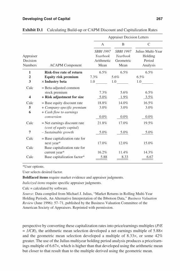
perspective by converting these capitalization rates into price/earnings multiples (P/E= 1/CR), the arithmetic mean selection developed a net earnings multiple of 5.88×and the geometric mean selection developed a multiple of 8.33×, or some 42%greater. The use of the Julius multiyear holding period analysis produces a price/earn-ings multiple of 6.67×, which is higher than that developed using the arithmetic meanbut closer to that result than to the multiple derived using the geometric mean.
Developing Cost of Capital 267
Exhibit D.1 Calculating Build-up or CAPM Discount and Capitalization Rates
Appraiser Decision Letters
A B C
SBBI 1997 SBBI 1997 Julius Multi-YearAppraiser Yearbook Yearbook HoldingDecision Arithmetic Geometric PeriodNumbers ACAPM Component Mean Mean Analysis
1 Risk-free rate of return 6.5% 6.5% 6.5%2 Equity risk premium 7.3% 5.6% 6.5%3 × Industry beta 1.0 1.0 1.0——— ——— ———
Calc = Beta-adjusted common stock premium 7.3% 5.6% 6.5%
4 + Risk adjustment for size 5.0% 1.9% 3.5%
Calc = Base equity discount rate 18.8% 14.0% 16.5%5 + Company-specific premium 3.0% 3.0% 3.0%6 + Cash flow to earnings
conversion 0.0% 0.0% 0.0%——— ——— ———Calc = Net earnings discount rate 21.8% 17.0% 19.5%
(cost of equity capital)7 – Sustainable growth 5.0% 5.0% 5.0%——— ——— ———
Calc = Base capitalization rate for next year* 17.0% 12.0% 15.0%
Calc Base capitalization rate for current year* 16.2% 11.4% 14.3%
Calc Base capitalization factor* 5.88 8.33 6.67——— ——— —————— ——— ———
*User options.
User selects desired factor.
Boldfaced items require market evidence and appraiser judgments.
Italicized items require specific appraiser judgments.
Calc = calculated by software.
Source: Data compiled from Michael J. Julius, “Market Returns in Rolling Multi-YearHolding Periods, An Alternative Interpretation of the Ibbotson Data,” Business ValuationReview (June 1996): 57–71, published by the Business Valuation Committee of theAmerican Society of Appraisers. Reprinted with permission.
3953 P-26 8/29/02 2:29 PM Page 267
My best advice to any appraiser, whether using ValuSource PRO or not, is to bevery clear at each of the numbered decision points (noted in Exhibit D.1) about whatmarket data are being used and why. Furthermore, appraisers should be clear aboutthe assumptions made regarding the lettered decision points in Exhibit D.1 as well.
Appraisers referring to the SBBI Yearbooks will develop components for thecommon stock equity premium, the appropriate beta, if applicable, and the small stockpremium. Those referring to the Grabowski/King analyses may have to calculate theimplied size premium in relationship to the base equity premiums initially used. Thepoint is that at numbered decision 4, the net size adjustment is developed by subtract-ing a total premium over Treasuries implied by Grabowski/King from the commonstock premium used in the analysis. In addition, appraisers may make a judgmentaladjustment for size in addition to any developed by Ibbotson, Grabowski/King, oranyone else—if their subject companies are substantially smaller than the publiccompanies used as reference points.
In the ValuSource PRO software, size premia are best considered in the “RiskAdjustment for Size” line. Appraisers using other than a so-called standard smallstock premium from Ibbotson should explain in their reports exactly how their sizepremia were developed.
Note that some appraisers have considered very small size as a company-specificrisk factor. There is nothing conceptually wrong with this treatment; however, beforedoing so, they should be familiar with current research on size premia or run the pos-sible risk of being viewed as arbitrary.
The company-specific premium is an integral part of the development of the costof equity capital. A breakout of several possible factors to consider in developing thispremium is provided in the software. There is no market evidence to help the appraiserdeal with most of these factors, and appraiser judgment must be carefully exercised.6
ValuSource PRO provides a line called “Cash Flow to Earnings Conversion.”Shannon Pratt has indicated that he believes that the CAPM (or ACAPM) discountrate is applicable to the net cash flow of a business enterprise. I have suggested thatit may be applicable to the net income of the enterprise. In Valuing Financial Insti-tutions, I prepared an analysis indicating a methodology for developing a conversionof a net cash flow discount rate to a net income discount rate, and suggested that formany private companies the differential might not be large.7 This analysis was alsoturned into an article that was published in the Business Valuation Review.8 Certainlyin the very long run, the net cash flow of an enterprise will approximate its net in-come. In any event, appraisers should be clear in their own minds what they believeon this issue and why, and then develop their remaining judgments consistently fromthis vantage point.
At this point, we have conceptually developed a net cash flow or net earningsdiscount rate. This discount rate is the equity cost of capital. This discount rate wouldbe applicable to projected net earnings in a discounted future earnings analysis (or,properly styled or adjusted, to the projected net cash flows in a discounted cash flowanalysis).
However, many appraisals are prepared without specific projections. To developa single-period capitalization rate, expected future earnings growth must be sub-tracted from the discount rate (for all the reasons explained earlier in this book).
268 Appendix D
3953 P-26 8/29/02 2:29 PM Page 268
EARNINGS STREAM TO BE CAPITALIZED
It should be fairly obvious that the discount rate or capitalization rate applied toany measure of earnings should be appropriately developed for that measure, whethernet income, pretax income, debt-free pretax income, or another level of the incomestatement. The CAPM discount rate discussed here and elsewhere in this book is gen-erally considered applicable to either the net income or the net cash flow of a busi-ness enterprise. In application in actual appraisals, however, a legitimate question canbe raised: To what net income or cash flow does the discount rate apply?
There has been considerable discussion in recent years regarding whether dis-counted future earnings (DFE) or discounted cash flow (DCF) valuation methods de-velop minority interest or controlling interest indications of value. A detailed discussionof the concept of levels of value is beyond the scope of this appendix; however, thequestion deserves some treatment.9
The two major trains of thought are as follows:
1. Since the CAPM discount rate is applicable to the net income of a business en-terprise, and since this discount rate is generally believed to develop value indi-cations at the marketable minority interest level of value, the value indicationfrom a discounted future cash flow or earnings valuation is a minority interest(marketable) conclusion. As a result, it would be proper to apply a control pre-mium to this value indication if a controlling interest conclusion is called for inthe appraisal.10
2. Since appraisers make so-called control adjustments in developing their projec-tions for DFE or DCF methods, the income stream is said to be control-adjusted,and the resulting valuation indication is at the controlling interest level.11
According to the first argument, buyers of companies might appear to have dif-ferent discount rates than hypothetical investors at the marketable minority interestlevel. According to the second argument, there is only one discount rate, and it is thesame for appraisers at the marketable minority interest level and for acquirers at thecontrolling interest level.
According to the first argument, one would add an appropriate control premiumto a DCF/DFE valuation method to arrive at a controlling interest level of value. Ac-cording to the second argument, a control premium might not be appropriate.
As is often the case, the truth may lie somewhere in between. To begin to resolvethe controversy, we can divide the so-called control adjustments into their two pri-mary component parts:
1. Normalizing Adjustments. In developing capitalization rates using data fromIbbotson Associates, Grabowski/King, or any other source of market return in-formation, there are implicit “market baskets” of publicly traded companiesthat constitute the basis of comparison with subject private companies. We knowthat the typical public company in a group is larger than many of the closely heldbusinesses that appraisers value, and this size differential gives rise to premium-required returns. We also know, generally, that public companies must pay
Developing Cost of Capital 269
3953 P-26 8/29/02 2:29 PM Page 269
competitive salaries to senior management or else run the risk of being penalizedin their market capitalizations. Likewise, related party transactions, to the extentthat they exist, must be conducted at arm’s length, and nonworking members ofthe president’s family are not normally found on the payroll of public companies.The point is that a significant portion of the control adjustments made in manyappraisals are, in reality, adjustments to normalize the earnings of the subjectcompany with the group of public companies with which it is implicitly beingcompared.
2. Acquirer’s Potential Economic (Control) Adjustments. Logically, an acquirerwould make the normalizing adjustments noted earlier in the context of an acqui-sition of a private company. Clearly, an owner is not going to be paid for the cap-italized value of excess salary and then continue to receive that salary. However,acquirers look at acquisition prospects differently than do public market securitiesinvestors. Acquirers often have an opportunity to generate economic benefits fromacquisitions that go beyond the normalizing adjustments noted earlier. For exam-ple, an acquirer in a similar business may be able to generate significant economiesby stripping out general and administrative or selling expenses from the acquiredentity. Alternatively, an acquirer may be able to generate economic benefits thatare not readily visible on a private company’s financial statements. For example,an acquirer may be willing to pay a premium for a business because of planned in-creased sales of existing products through the acquired company’s sales force.These types of potential economic benefits (adjustments) may generate the will-ingness to pay an apparent control premium for a company that otherwise mightnot be immediately justified.
The example in Exhibit D.2 illustrates a delineation of potential valuation adjust-ments into those categorized as normalizing (Line 2) and those noted as economic(control) adjustments made by a potential acquirer of control (Line 3).
In most appraisals, the adjustments made normally fall into the category of nor-malizing adjustments. The analysis in Exhibit D.2 indicates that it is not at all incon-sistent to suggest that the discount rates are the same for the potential buyer of acompany as for the hypothetical willing buyer of a marketable minority interest. (SeeLine 7, where the same price/earnings multiple and, implicitly, discount rate, is ap-plied to differing perceptions of a subject company’s earnings.) This would suggest,however, that the economic benefits of control have not yet been factored into the ap-praisal process at the marketable minority interest level, and that a control premiummay be necessary to reach a proper conclusion of value on a controlling interest basis(see Line 10, where the implied control premium is 20%).
In the alternative, the appraiser would estimate these economic benefits specifi-cally and capitalize them to develop a controlling interest conclusion. In the example inExhibit D.2, the control premium provides a vehicle to estimate the magnitude of thebenefit of potential economic (control) adjustments and to reflect them in the appraisal.
For users of ValuSource PRO software, the message is clear. Be sure to under-stand what adjustments have been made in an appraisal. To the extent that the nor-malizing adjustments of an appraisal do not consider the potential economic benefits
270 Appendix D
3953 P-26 8/29/02 2:29 PM Page 270
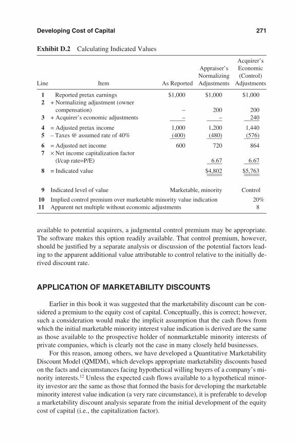
available to potential acquirers, a judgmental control premium may be appropriate.The software makes this option readily available. That control premium, however,should be justified by a separate analysis or discussion of the potential factors lead-ing to the apparent additional value attributable to control relative to the initially de-rived discount rate.
APPLICATION OF MARKETABILITY DISCOUNTS
Earlier in this book it was suggested that the marketability discount can be con-sidered a premium to the equity cost of capital. Conceptually, this is correct; however,such a consideration would make the implicit assumption that the cash flows fromwhich the initial marketable minority interest value indication is derived are the sameas those available to the prospective holder of nonmarketable minority interests ofprivate companies, which is clearly not the case in many closely held businesses.
For this reason, among others, we have developed a Quantitative MarketabilityDiscount Model (QMDM), which develops appropriate marketability discounts basedon the facts and circumstances facing hypothetical willing buyers of a company’s mi-nority interests.12 Unless the expected cash flows available to a hypothetical minor-ity investor are the same as those that formed the basis for developing the marketableminority interest value indication (a very rare circumstance), it is preferable to developa marketability discount analysis separate from the initial development of the equitycost of capital (i.e., the capitalization factor).
Developing Cost of Capital 271
Exhibit D.2 Calculating Indicated Values
Acquirer’sAppraiser’s EconomicNormalizing (Control)
Line Item As Reported Adjustments Adjustments
1 Reported pretax earnings $1,000 $1,000 $1,0002 + Normalizing adjustment (owner
compensation) – 200 2003 + Acquirer’s economic adjustments – – 240—–— —–— —–—4 = Adjusted pretax income 1,000 1,200 1,4405 – Taxes @ assumed rate of 40% (400) (480) (576)—–— —–— —–—6 = Adjusted net income 600 720 8647 × Net income capitalization factor
(l/cap rate=P/E) 6.67 6.67—–— —–—8 = Indicated value $4,802 $5,763—–— —–——–— —–—
9 Indicated level of value Marketable, minority Control
10 Implied control premium over marketable minority value indication 20%11 Apparent net multiple without economic adjustments 8
3953 P-26 8/29/02 2:29 PM Page 271
Wiley ValuSource offers the QMDM in a CD-ROM format. The resultant dis-counts from this CD-ROM product can be incorporated into ValuSource PRO (Ver-sions 2001, 2000, and 1.06).13
Notes
1. ASA Business Valuation Standards and Portions of Uniform Standards of ProfessionalAppraisal Practice (USPAP) (Herndon, VA: American Society of Appraisers, revisedJanuary 1994), 18.
2. Z. Christopher Mercer, “The Adjusted Capital Asset Pricing Model for Developing Capi-talization Rates: An Extension of Previous ‘Build-Up’ Methodologies Based upon the Cap-ital Asset Pricing Model,” Business Valuation Review (December 1989): 147–156. Also seeChapter 13 in Z. Christopher Mercer, Valuing Financial Institutions (Burr Ridge, IL:McGraw-Hill, 1992), and Exhibit 8.2 in Z. Christopher Mercer, Quantifying MarketabilityDiscounts: Developing and Supporting Marketability Discounts in the Appraisal of CloselyHeld Business Interests, revised reprint (Memphis, TN: Peabody Publishing, LP, 2001).Quantifying Marketability Discounts is available from the publisher at 800-769-0967.
3. Stocks, Bonds, Bills and Inflation, Classic Edition and Valuation Edition, published an-nually; Cost of Capital Yearbook, published annually with quarterly updates; and BetaBook, published semiannually. Chicago: Ibbotson Associates.
4. Roger Grabowski and David King, “Size Effects and Equity Returns, An Update,” Busi-ness Valuation Review (March 1997): 22–26. Discussed in Shannon Pratt’s BusinessValuation Update® (August 1997): 1.
5. J. Michael Julius, “Market Returns in Rolling Multi-Year Holding Periods: An Alterna-tive Interpretation of the Ibbotson Data,” Business Valuation Review (June 1996): 57–71.There has been something of a controversy over whether the more appropriate averagestatistics from Ibbotson’s SBBI Yearbook is the arithmetic mean or the geometric mean.At its simplest, the Julius analysis recognizes that the arithmetic mean of the Ibbotson re-turn data from 1926 to 1997 is the arithmetic mean (average) of 71 annual returns. The an-nual returns are the geometric means of the annual observations. So the arithmetic meanadvanced by Ibbotson Associates is the arithmetic mean of 71 annual (geometric) returns,reflecting 71 one-year holding periods. The geometric mean advanced by others is sim-ply the compound growth rate in total return from 1926 to 1997, or the geometric meanreturn for the period, which represents a single, 71-year holding period. From a practicalviewpoint, neither extreme makes logical sense (and I am oversimplifying complex log-ical arguments to be practical). The Julius analysis examines the arithmetic mean of geo-metric returns for multiyear holding periods that have occurred from 1926 to 1995 (in thecited article). The effect of this averaging process over many multiyear holding periodsis to develop a series of average returns for more reasonable holding periods such as, say,five or 10 years. The result, incidentally, is effectively to split the difference between thearithmetic mean and the geometric mean as calculated by Ibbotson. We have used thisanalysis for years as a basis for determining the appropriate common stock and smallstock premium return measures.
6. As the appraisal profession matures, various appraisers are creatively examining the pub-lic stock markets for guidance on fundamental issues like developing company-specificrisk premiums. A recent article typifies these efforts: Steven Bolten and Yan Wang, “TheImpact of Management Depth on Valuation,” Business Valuation Review (September1997): 143–146.
272 Appendix D
3953 P-26 8/29/02 2:29 PM Page 272

7. See Mercer, Valuing Financial Institutions, Exhibit 14.7, 262–266.8. Z. Christopher Mercer, “Adjusted Capitalization Rates for the Difference Between Net In-
come and Net Free Cash Flow,” Business Valuation Review (December 1992): 201–207.9. See Mercer, Quantifying Marketability Discounts, Revised Reprint, Chapter 1.
10. See Estate of Jung v. Commissioner for a discussion of this argument, 101 T.C. 412 (U.S.Tax Ct. 1993).
11. See Chapter 13 of this book, written by Michael W. Barad and Tara McDowell of Ibbot-son Associates, for elements of this argument.
12. See Mercer, Quantifying Marketability Discount, Revised Reprint, Chapter 8.13. Z. Christopher Mercer, “Quantifying Marketability Discount Modeling,” Wiley ValuSource
(software), 1-800-825-8763.
Developing Cost of Capital 273
3953 P-26 8/29/02 2:29 PM Page 273
274
Appendix E
Iterative Process UsingCAPM to Calculate the Cost of Equity Component ofthe Weighted Average Costof Capital1
Harold G. Martin, Jr., MBA, CPA/ABV, ASA, CFE
OverviewCapital Asset Pricing Model and BetaSolution—The Iterative Process
IterationIterative Process Using a Financial Spreadsheet Model
Iteration 1Iteration 2Iteration 3Iteration 4
SummaryAdditional Reading
OVERVIEW
In Chapter 7 Dr. Pratt presents an iterative process for computing the weightedaverage cost of capital (WACC) for a closely held company. In determining theWACC, the market values of the capital structure components—that is, debt and eq-uity—are required to determine the relative weights of each component. However,this sets up a “catch-22” scenario:
• Our objective is to determine the market value of equity for the closely held com-pany based on some unknown WACC.
• To determine the WACC, we must solve for an unknown market value of equity.
Chapter 7 presents an estimation technique, the iterative process, that provides amethod for circumventing this problem. This appendix expands on the technique and
3953 P-27 8/29/02 2:29 PM Page 274
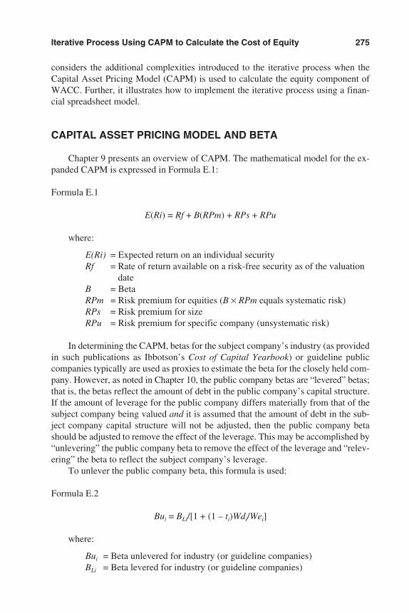
considers the additional complexities introduced to the iterative process when theCapital Asset Pricing Model (CAPM) is used to calculate the equity component ofWACC. Further, it illustrates how to implement the iterative process using a finan-cial spreadsheet model.
CAPITAL ASSET PRICING MODEL AND BETA
Chapter 9 presents an overview of CAPM. The mathematical model for the ex-panded CAPM is expressed in Formula E.1:
Formula E.1
E(Ri) = Rf + B(RPm) + RPs + RPu
where:
E(Ri) = Expected return on an individual securityRf = Rate of return available on a risk-free security as of the valuation
dateB = BetaRPm = Risk premium for equities (B × RPm equals systematic risk)RPs = Risk premium for sizeRPu = Risk premium for specific company (unsystematic risk)
In determining the CAPM, betas for the subject company’s industry (as providedin such publications as Ibbotson’s Cost of Capital Yearbook) or guideline publiccompanies typically are used as proxies to estimate the beta for the closely held com-pany. However, as noted in Chapter 10, the public company betas are “levered” betas;that is, the betas reflect the amount of debt in the public company’s capital structure.If the amount of leverage for the public company differs materially from that of thesubject company being valued and it is assumed that the amount of debt in the sub-ject company capital structure will not be adjusted, then the public company betashould be adjusted to remove the effect of the leverage. This may be accomplished by“unlevering” the public company beta to remove the effect of the leverage and “relev-ering” the beta to reflect the subject company’s leverage.
To unlever the public company beta, this formula is used:
Formula E.2
Bui = BLi/[1 + (1 – ti)Wdi/Wei]
where:
Bui = Beta unlevered for industry (or guideline companies)BLi = Beta levered for industry (or guideline companies)
Iterative Process Using CAPM to Calculate the Cost of Equity 275
3953 P-27 8/29/02 2:29 PM Page 275
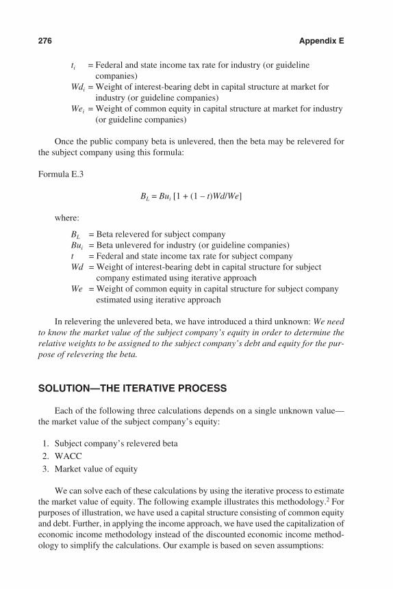
ti = Federal and state income tax rate for industry (or guidelinecompanies)
Wdi = Weight of interest-bearing debt in capital structure at market forindustry (or guideline companies)
Wei = Weight of common equity in capital structure at market for industry(or guideline companies)
Once the public company beta is unlevered, then the beta may be relevered forthe subject company using this formula:
Formula E.3
BL = Bui [1 + (1 – t)Wd/We]
where:
BL = Beta relevered for subject companyBui = Beta unlevered for industry (or guideline companies)t = Federal and state income tax rate for subject companyWd = Weight of interest-bearing debt in capital structure for subject
company estimated using iterative approachWe = Weight of common equity in capital structure for subject company
estimated using iterative approach
In relevering the unlevered beta, we have introduced a third unknown: We needto know the market value of the subject company’s equity in order to determine therelative weights to be assigned to the subject company’s debt and equity for the pur-pose of relevering the beta.
SOLUTION—THE ITERATIVE PROCESS
Each of the following three calculations depends on a single unknown value—the market value of the subject company’s equity:
1. Subject company’s relevered beta
2. WACC
3. Market value of equity
We can solve each of these calculations by using the iterative process to estimatethe market value of equity. The following example illustrates this methodology.2 Forpurposes of illustration, we have used a capital structure consisting of common equityand debt. Further, in applying the income approach, we have used the capitalization ofeconomic income methodology instead of the discounted economic income method-ology to simplify the calculations. Our example is based on seven assumptions:
276 Appendix E
3953 P-27 8/29/02 2:29 PM Page 276
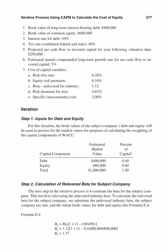
1. Book value of long-term interest-bearing debt: $400,000
2. Book value of common equity: $600,000
3. Interest rate for debt: 10%
4. Tax rate (combined federal and state): 40%
5. Projected net cash flow to invested capital for year following valuation date:$250,000
6. Estimated annual compounded long-term growth rate for net cash flow to in-vested capital: 5%
7. Cost of capital variables:
a. Risk-free rate: 6.28%
b. Equity risk premium: 8.10%
c. Beta—unlevered for industry: 1.12
d. Risk premium for size: 4.63%
e. Specific (unsystematic) risk: 2.00%
Iteration
Step 1. Inputs for Debt and Equity
For this iteration, the book values of the subject company’s debt and equity willbe used as proxies for the market values for purposes of calculating the weighting ofthe capital components of WACC:
Estimated PercentMarket of
Capital Component Value Capital3
Debt $400,000 0.40Equity 600,000 0.60Total $1,000,000 1.00
Step 2. Calculation of Relevered Beta for Subject Company
The next step in the iterative process is to estimate the beta for the subject com-pany. This involves relevering the unlevered industry beta. To calculate the releveredbeta for the subject company, we substitute the unlevered industry beta, the subjectcompany tax rate, and the initial book values for debt and equity into Formula E.4:
Formula E.4
BL = Bui[1 + (1 – t)Wd/We]BL = 1.12[1 + (1 – 0.4)400,000/600,000]BL = 1.57
Iterative Process Using CAPM to Calculate the Cost of Equity 277
3953 P-27 8/29/02 2:29 PM Page 277
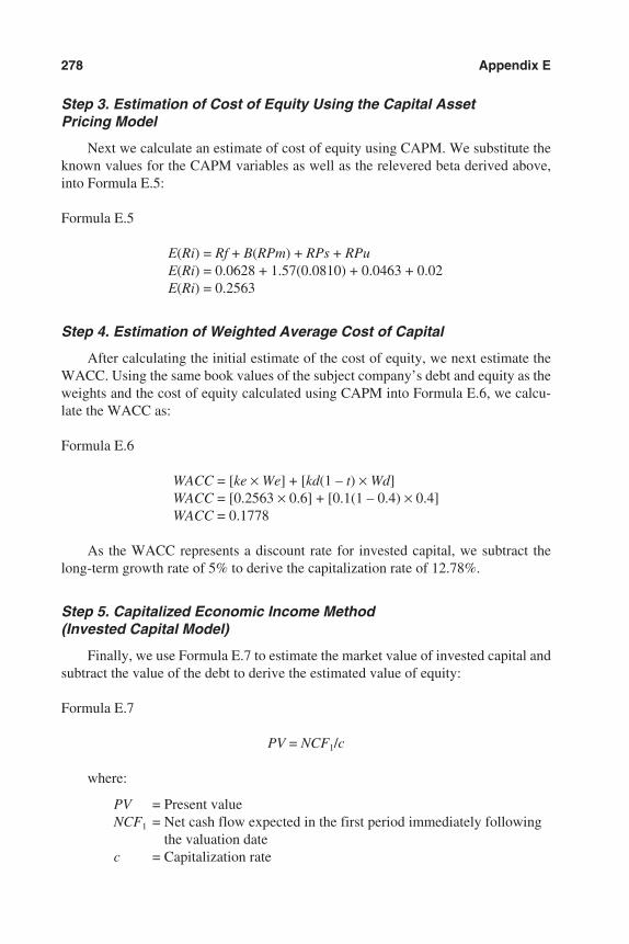
Step 3. Estimation of Cost of Equity Using the Capital Asset Pricing Model
Next we calculate an estimate of cost of equity using CAPM. We substitute theknown values for the CAPM variables as well as the relevered beta derived above,into Formula E.5:
Formula E.5
E(Ri) = Rf + B(RPm) + RPs + RPuE(Ri) = 0.0628 + 1.57(0.0810) + 0.0463 + 0.02E(Ri) = 0.2563
Step 4. Estimation of Weighted Average Cost of Capital
After calculating the initial estimate of the cost of equity, we next estimate theWACC. Using the same book values of the subject company’s debt and equity as theweights and the cost of equity calculated using CAPM into Formula E.6, we calcu-late the WACC as:
Formula E.6
WACC = [ke × We] + [kd(1 – t) × Wd]WACC = [0.2563 × 0.6] + [0.1(1 – 0.4) × 0.4]WACC = 0.1778
As the WACC represents a discount rate for invested capital, we subtract thelong-term growth rate of 5% to derive the capitalization rate of 12.78%.
Step 5. Capitalized Economic Income Method (Invested Capital Model)
Finally, we use Formula E.7 to estimate the market value of invested capital andsubtract the value of the debt to derive the estimated value of equity:
Formula E.7
PV = NCF1/c
where:
PV = Present valueNCF1 = Net cash flow expected in the first period immediately following
the valuation datec = Capitalization rate
278 Appendix E
3953 P-27 8/29/02 2:29 PM Page 278
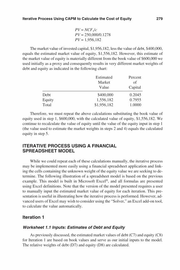
PV = NCF1/cPV = 250,000/0.1278PV = 1,956,182
The market value of invested capital, $1,956,182, less the value of debt, $400,000,equals the estimated market value of equity, $1,556,182. However, this estimate ofthe market value of equity is materially different from the book value of $600,000 weused initially as a proxy and consequently results in very different market weights ofdebt and equity as indicated in the following chart:
Estimated PercentMarket ofValue Capital
Debt $400,000 0.2045Equity 1,556,182 0.7955Total $1,956,182 1.0000
Therefore, we must repeat the above calculations substituting the book value ofequity used in step 1, $600,000, with the calculated value of equity, $1,556,182. Wecontinue to recalculate the value of equity until the value of the equity input in step 1(the value used to estimate the market weights in steps 2 and 4) equals the calculatedequity in step 5.
ITERATIVE PROCESS USING A FINANCIAL SPREADSHEET MODEL
While we could repeat each of these calculations manually, the iterative processmay be implemented more easily using a financial spreadsheet application and link-ing the cells containing the unknown weight of the equity value we are seeking to de-termine. The following illustration of a spreadsheet model is based on the previousexample. This model is built in Microsoft Excel®, and all formulas are presentedusing Excel definitions. Note that the version of the model presented requires a userto manually input the estimated market value of equity for each iteration. This pre-sentation is useful in illustrating how the iterative process is performed. However, ad-vanced users of Excel may wish to consider using the “Solver,” an Excel add-on tool,to calculate the value automatically.
Iteration 1
Worksheet 1.1 Inputs: Estimates of Debt and Equity
As previously discussed, the estimated market values of debt (C7) and equity (C8)for Iteration 1 are based on book values and serve as our initial inputs to the model.The relative weights of debt (D7) and equity (D8) are calculated.
Iterative Process Using CAPM to Calculate the Cost of Equity 279
3953 P-27 8/29/02 2:29 PM Page 279
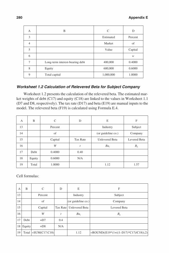
A B C D
3 Estimated Percent
4 Market of
5 Value Capital
6 w
7 Long-term interest-bearing debt 400,000 0.4000
8 Equity 600,000 0.6000
9 Total capital 1,000,000 1.0000
Worksheet 1.2 Calculation of Relevered Beta for Subject Company
Worksheet 1.2 presents the calculation of the relevered beta. The estimated mar-ket weights of debt (C17) and equity (C18) are linked to the values in Worksheet 1.1(D7 and D8, respectively). The tax rate (D17) and beta (E19) are manual inputs to themodel. The relevered beta (F19) is calculated using Formula E.4.
A B C D E F
13 Percent Industry Subject
14 of (or guideline co.) Company
15 Capital Tax Rate Unlevered Beta Levered Beta
16 W t Bui BL
17 Debt 0.4000 0.40
18 Equity 0.6000 N/A
19 Total 1.0000 1.12 1.57
Cell formulas:
A B C D E F
13 Percent Industry Subject
14 of (or guideline co.) Company
15 Capital Tax Rate Unlevered Beta Levered Beta
16 W t Bui BL
17 Debt =D7 0.4
18 Equity =D8 N/A
19 Total =SUM(C17:C18) 1.12 =ROUND((E19*(1+((1–D17)*C17)/C18)),2)
280 Appendix E
3953 P-27 8/29/02 2:29 PM Page 280
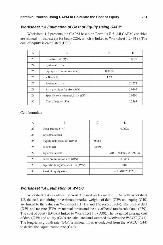
Worksheet 1.3 Estimation of Cost of Equity Using CAPM
Worksheet 1.3 presents the CAPM based on Formula E.5. All CAPM variablesare manual inputs, except for beta (C26), which is linked to Worksheet 1.2 (F19). Thecost of equity is calculated (D30).
A B C D
23 Risk-free rate (Rf) 0.0628
24 Systematic risk
25 Equity risk premium (RPm) 0.0810
26 × Beta (B) 1.57
27 Systematic risk 0.1272
28 Risk premium for size (RPs) 0.0463
29 Specific (unsystematic) risk (RPu) 0.0200
30 Cost of equity (Ke) 0.2563
Cell formulas:
A B C D
23 Risk-free rate (Rf) 0.0628
24 Systematic risk
25 Equity risk premium (RPm) 0.081
26 × Beta (B) =F19
27 Systematic risk =ROUND((C25*C26),4)
28 Risk premium for size (RPs) 0.0463
29 Specific (unsystematic) risk (RPu) 0.02
30 Cost of equity (Ke) =SUM(D23:D29)
Worksheet 1.4 Estimation of WACC
Worksheet 1.4 calculates the WACC based on Formula E.6. As with Worksheet1.2, the cells containing the estimated market weights of debt (C39) and equity (C40)are linked to the values in Worksheet 1.1 (D7 and D8, respectively). The cost of debt(D39) and tax rate (E39) are manual inputs and the tax-affected rate is calculated (F39).The cost of equity (D40) is linked to Worksheet 1.3 (D30). The weighted average costof debt (G39) and equity (G40) are calculated and summed to derive the WACC (G41).The long-term growth rate (G45), a manual input, is deducted from the WACC (G44)to derive the capitalization rate (G46).
Iterative Process Using CAPM to Calculate the Cost of Equity 281
3953 P-27 8/29/02 2:29 PM Page 281
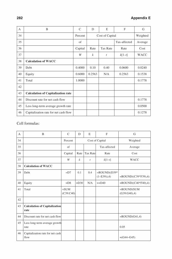
A B C D E F G
34 Percent Cost of Capital Weighted
35 of Tax-affected Average
36 Capital Rate Tax Rate Rate Cost
37 W k t k[1–t] WACC
38 Calculation of WACC
39 Debt 0.4000 0.10 0.40 0.0600 0.0240
40 Equity 0.6000 0.2563 N/A 0.2563 0.1538
41 Total 1.0000 0.1778
42
43 Calculation of Capitalization rate
44 Discount rate for net cash flow 0.1778
45 Less long-term average growth rate 0.0500
46 Capitalization rate for net cash flow 0.1278
Cell formulas:
A B C D E F G
34 Percent Cost of Capital Weighted
35 of Tax-affected Average
36 Capital Rate Tax Rate Rate Cost
37 W k t k[1–t] WACC
38 Calculation of WACC
39 Debt =D7 0.1 0.4 =ROUND((D39*(1–E39)),4) =ROUND((C39*F39),4)
40 Equity =D8 =D30 N/A =+D40 =ROUND((C40*F40),4)
41 Total =SUM =ROUND(SUM(C39:C40) (G39:G40),4)
42
43 Calculation of Capitalization rate
44 Discount rate for net cash flow =ROUND(G41,4)
45 Less long-term average growth rate 0.05
46 Capitalization rate for net cash flow =(G44–G45)
282 Appendix E
3953 P-27 8/29/02 2:29 PM Page 282
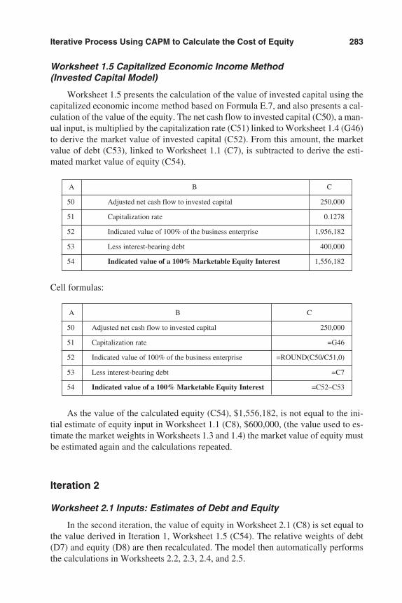
Worksheet 1.5 Capitalized Economic Income Method (Invested Capital Model)
Worksheet 1.5 presents the calculation of the value of invested capital using thecapitalized economic income method based on Formula E.7, and also presents a cal-culation of the value of the equity. The net cash flow to invested capital (C50), a man-ual input, is multiplied by the capitalization rate (C51) linked to Worksheet 1.4 (G46)to derive the market value of invested capital (C52). From this amount, the marketvalue of debt (C53), linked to Worksheet 1.1 (C7), is subtracted to derive the esti-mated market value of equity (C54).
A B C
50 Adjusted net cash flow to invested capital 250,000
51 Capitalization rate 0.1278
52 Indicated value of 100% of the business enterprise 1,956,182
53 Less interest-bearing debt 400,000
54 Indicated value of a 100% Marketable Equity Interest 1,556,182
Cell formulas:
A B C
50 Adjusted net cash flow to invested capital 250,000
51 Capitalization rate =G46
52 Indicated value of 100% of the business enterprise =ROUND(C50/C51,0)
53 Less interest-bearing debt =C7
54 Indicated value of a 100% Marketable Equity Interest =C52–C53
As the value of the calculated equity (C54), $1,556,182, is not equal to the ini-tial estimate of equity input in Worksheet 1.1 (C8), $600,000, (the value used to es-timate the market weights in Worksheets 1.3 and 1.4) the market value of equity mustbe estimated again and the calculations repeated.
Iteration 2
Worksheet 2.1 Inputs: Estimates of Debt and Equity
In the second iteration, the value of equity in Worksheet 2.1 (C8) is set equal tothe value derived in Iteration 1, Worksheet 1.5 (C54). The relative weights of debt(D7) and equity (D8) are then recalculated. The model then automatically performsthe calculations in Worksheets 2.2, 2.3, 2.4, and 2.5.
Iterative Process Using CAPM to Calculate the Cost of Equity 283
3953 P-27 8/29/02 2:29 PM Page 283
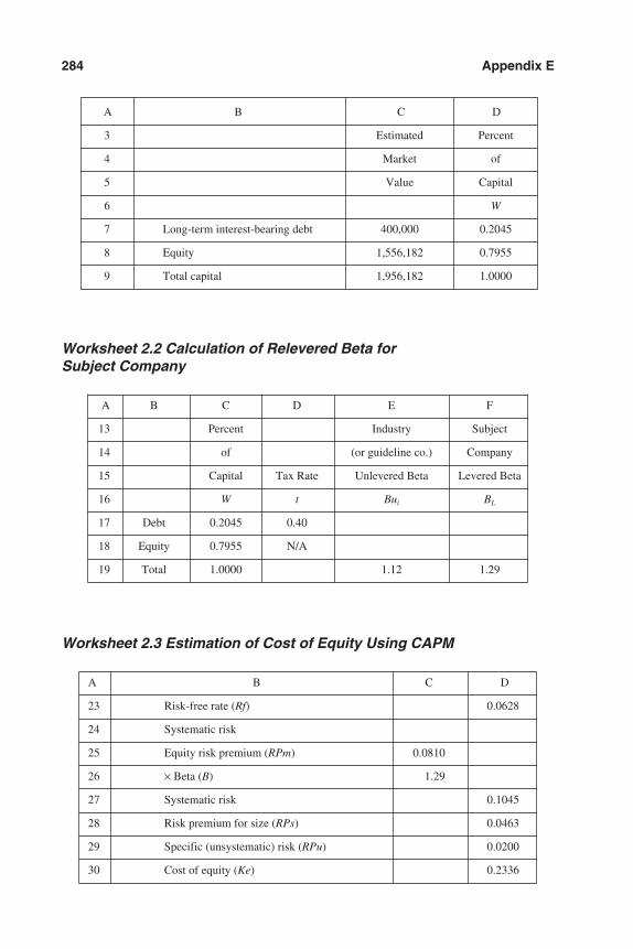
Worksheet 2.2 Calculation of Relevered Beta for Subject Company
A B C D E F
13 Percent Industry Subject
14 of (or guideline co.) Company
15 Capital Tax Rate Unlevered Beta Levered Beta
16 W t Bui BL
17 Debt 0.2045 0.40
18 Equity 0.7955 N/A
19 Total 1.0000 1.12 1.29
Worksheet 2.3 Estimation of Cost of Equity Using CAPM
A B C D
23 Risk-free rate (Rf) 0.0628
24 Systematic risk
25 Equity risk premium (RPm) 0.0810
26 × Beta (B) 1.29
27 Systematic risk 0.1045
28 Risk premium for size (RPs) 0.0463
29 Specific (unsystematic) risk (RPu) 0.0200
30 Cost of equity (Ke) 0.2336
284 Appendix E
A B C D
3 Estimated Percent
4 Market of
5 Value Capital
6 W
7 Long-term interest-bearing debt 400,000 0.2045
8 Equity 1,556,182 0.7955
9 Total capital 1,956,182 1.0000
3953 P-27 8/29/02 2:29 PM Page 284
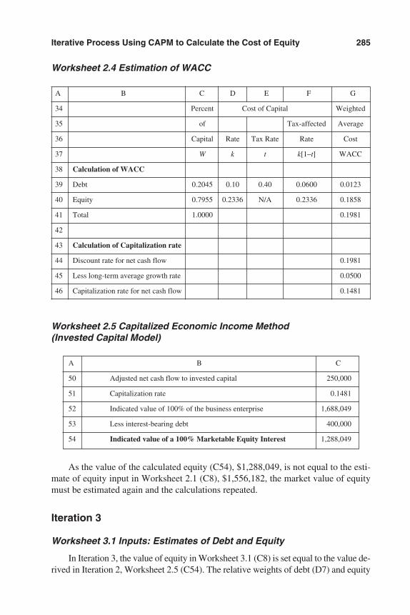
Worksheet 2.4 Estimation of WACC
A B C D E F G
34 Percent Cost of Capital Weighted
35 of Tax-affected Average
36 Capital Rate Tax Rate Rate Cost
37 W k t k[1–t] WACC
38 Calculation of WACC
39 Debt 0.2045 0.10 0.40 0.0600 0.0123
40 Equity 0.7955 0.2336 N/A 0.2336 0.1858
41 Total 1.0000 0.1981
42
43 Calculation of Capitalization rate
44 Discount rate for net cash flow 0.1981
45 Less long-term average growth rate 0.0500
46 Capitalization rate for net cash flow 0.1481
Worksheet 2.5 Capitalized Economic Income Method (Invested Capital Model)
A B C
50 Adjusted net cash flow to invested capital 250,000
51 Capitalization rate 0.1481
52 Indicated value of 100% of the business enterprise 1,688,049
53 Less interest-bearing debt 400,000
54 Indicated value of a 100% Marketable Equity Interest 1,288,049
As the value of the calculated equity (C54), $1,288,049, is not equal to the esti-mate of equity input in Worksheet 2.1 (C8), $1,556,182, the market value of equitymust be estimated again and the calculations repeated.
Iteration 3
Worksheet 3.1 Inputs: Estimates of Debt and Equity
In Iteration 3, the value of equity in Worksheet 3.1 (C8) is set equal to the value de-rived in Iteration 2, Worksheet 2.5 (C54). The relative weights of debt (D7) and equity
Iterative Process Using CAPM to Calculate the Cost of Equity 285
3953 P-27 8/29/02 2:29 PM Page 285

(D8) are then recalculated. The model then automatically performs the calculations inWorksheets 3.2, 3.3, 3.4, and 3.5.
A B C D
3 Estimated Percent
4 Market of
5 Value Capital
6 W
7 Long-term interest-bearing debt 400,000 0.2370
8 Equity 1,288,049 0.7630
9 Total capital 1,688,049 1.0000
Worksheet 3.2 Calculation of Relevered Beta for Subject Company
A B C D E F
13 Percent Industry Subject
14 of (or guideline co.) Company
15 Capital Tax Rate Unlevered Beta Levered Beta
16 W t Bui BL
17 Debt 0.2370 0.40
18 Equity 0.7630 N/A
19 Total 1.0000 1.12 1.33
Worksheet 3.3 Estimation of Cost of Equity Using CAPM
A B C D
23 Risk-free rate (Rf) 0.0628
24 Systematic risk
25 Equity risk premium (RPm) 0.0810
26 × Beta (B) 1.33
27 Systematic risk 0.1077
28 Risk premium for size (RPs) 0.0463
29 Specific (unsystematic) risk (RPu) 0.0200
30 Cost of equity (Ke) 0.2368
286 Appendix E
3953 P-27 8/29/02 2:29 PM Page 286
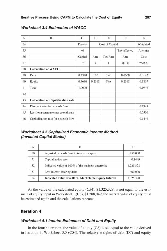
Worksheet 3.4 Estimation of WACC
A B C D E F G
34 Percent Cost of Capital Weighted
35 of Tax-affected Average
36 Capital Rate Tax Rate Rate Cost
37 W k t k[1–t] WACC
38 Calculation of WACC
39 Debt 0.2370 0.10 0.40 0.0600 0.0142
40 Equity 0.7630 0.2368 N/A 0.2368 0.1807
41 Total 1.0000 0.1949
42
43 Calculation of Capitalization rate
44 Discount rate for net cash flow 0.1949
45 Less long-term average growth rate 0.0500
46 Capitalization rate for net cash flow 0.1449
Worksheet 3.5 Capitalized Economic Income Method (Invested Capital Model)
A B C
50 Adjusted net cash flow to invested capital 250,000
51 Capitalization rate 0.1449
52 Indicated value of 100% of the business enterprise 1,725,328
53 Less interest-bearing debt 400,000
54 Indicated value of a 100% Marketable Equity Interest 1,325,328
As the value of the calculated equity (C54), $1,325,328, is not equal to the esti-mate of equity input in Worksheet 1 (C8), $1,288,049, the market value of equity mustbe estimated again and the calculations repeated.
Iteration 4
Worksheet 4.1 Inputs: Estimates of Debt and Equity
In the fourth iteration, the value of equity (C8) is set equal to the value derivedin Iteration 3, Worksheet 3.5 (C54). The relative weights of debt (D7) and equity
Iterative Process Using CAPM to Calculate the Cost of Equity 287
3953 P-27 8/29/02 2:29 PM Page 287
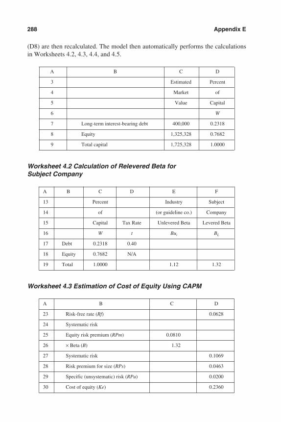
(D8) are then recalculated. The model then automatically performs the calculationsin Worksheets 4.2, 4.3, 4.4, and 4.5.
A B C D
3 Estimated Percent
4 Market of
5 Value Capital
6 W
7 Long-term interest-bearing debt 400,000 0.2318
8 Equity 1,325,328 0.7682
9 Total capital 1,725,328 1.0000
Worksheet 4.2 Calculation of Relevered Beta for Subject Company
A B C D E F
13 Percent Industry Subject
14 of (or guideline co.) Company
15 Capital Tax Rate Unlevered Beta Levered Beta
16 W t Bui BL
17 Debt 0.2318 0.40
18 Equity 0.7682 N/A
19 Total 1.0000 1.12 1.32
Worksheet 4.3 Estimation of Cost of Equity Using CAPM
A B C D
23 Risk-free rate (Rf) 0.0628
24 Systematic risk
25 Equity risk premium (RPm) 0.0810
26 × Beta (B) 1.32
27 Systematic risk 0.1069
28 Risk premium for size (RPs) 0.0463
29 Specific (unsystematic) risk (RPu) 0.0200
30 Cost of equity (Ke) 0.2360
288 Appendix E
3953 P-27 8/29/02 2:29 PM Page 288
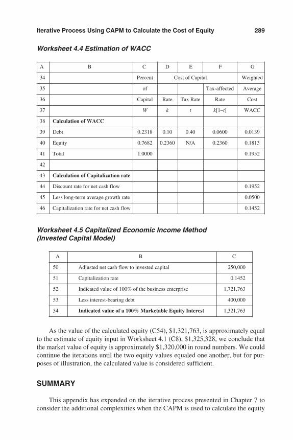
Worksheet 4.4 Estimation of WACC
A B C D E F G
34 Percent Cost of Capital Weighted
35 of Tax-affected Average
36 Capital Rate Tax Rate Rate Cost
37 W k t k[1–t] WACC
38 Calculation of WACC
39 Debt 0.2318 0.10 0.40 0.0600 0.0139
40 Equity 0.7682 0.2360 N/A 0.2360 0.1813
41 Total 1.0000 0.1952
42
43 Calculation of Capitalization rate
44 Discount rate for net cash flow 0.1952
45 Less long-term average growth rate 0.0500
46 Capitalization rate for net cash flow 0.1452
Worksheet 4.5 Capitalized Economic Income Method (Invested Capital Model)
A B C
50 Adjusted net cash flow to invested capital 250,000
51 Capitalization rate 0.1452
52 Indicated value of 100% of the business enterprise 1,721,763
53 Less interest-bearing debt 400,000
54 Indicated value of a 100% Marketable Equity Interest 1,321,763
As the value of the calculated equity (C54), $1,321,763, is approximately equalto the estimate of equity input in Worksheet 4.1 (C8), $1,325,328, we conclude thatthe market value of equity is approximately $1,320,000 in round numbers. We couldcontinue the iterations until the two equity values equaled one another, but for pur-poses of illustration, the calculated value is considered sufficient.
SUMMARY
This appendix has expanded on the iterative process presented in Chapter 7 toconsider the additional complexities when the CAPM is used to calculate the equity
Iterative Process Using CAPM to Calculate the Cost of Equity 289
3953 P-27 8/29/02 2:29 PM Page 289
component of WACC. Further, it has provided an example illustrating the use of a fi-nancial spreadsheet model to perform the calculations required for the iterativeprocess.
Notes
1. In developing the model presented here, I have received invaluable guidance from profes-sional colleagues and resources such as the first edition of Cost of Capital. In particular, Iwish to thank James R. Hitchner of Phillips Hitchner in Atlanta, Georgia, for sparking myinitial interest in the invested capital valuation methodology, and Mark L. Zyla, also ofPhillips Hitchner in Atlanta, Georgia, and Michael J. Mattson of The Financial ValuationGroup in Chicago, Illinois, for their suggestions and critique of the model. Any errors re-lating to its application are solely my own. This model was first introduced in a presentationentitled “Cost of Capital” at the American Institute of Certified Public Accountants NationalBusiness Valuation Conference, December 4, 2001.
2. The example used in the illustration is based on a presentation entitled “Cost of Capital”presented at the American Institute of Certified Public Accountants National BusinessValuation Conference, December 4, 2001. I have modified the example to mirror the ex-ample presented in Chapter 7, with the exception that I have expanded on it to illustratethe derivation of a relevered beta and the use of CAPM in deriving the cost of equity com-ponent of the WACC.
3. Percentages are expressed as decimal equivalents.
ADDITIONAL READING
Abrams, Jay B. Quantitative Business Valuation: A Mathematical Approach forToday’s Professionals. New York: McGraw-Hill, 2001.
Adams, David P., et al. Fundamentals of Business Valuation: Part I. Lewisville, TX:American Institute of Certified Public Accountants, 2001.
Annin, Michael, and Dominic Falaschetti. Stocks, Bonds, Bills, and Inflation Valua-tion Edition 2001 Yearbook. Chicago: Ibbotson Associates, 2001.
Bishop, David M., and Frank C. Evans. “Avoiding a Common Error in Calculatingthe Weighted Average Cost of Capital.” CPA Expert. New York: American Insti-tute of Certified Public Accountants (fall 1997).
Evans, Frank C., and Kelly L. Strimbu. “Debt and Equity Weightings in WACC.”CPA Expert. New York: American Institute of Certified Public Accountants (fall1998).
Hitchner, James R., et al, Financial Valuation: Application and Models. New York:John Wiley & Sons, Inc., forthcoming.
Ibbotson Associates Cost of Capital 2001 Yearbook. Chicago: Ibbotson Associates,2001.
290 Appendix E
3953 P-27 8/29/02 2:29 PM Page 290

Martin, Harold G., Jr. “Cost of Capital.” Joint presentation made with Ronald L.Seigneur at the American Institute of Certified Public Accountants National Busi-ness Valuation Conference, Las Vegas, NV, December 4, 2001.
Pratt, Shannon P., et al. Valuing a Business: The Analysis and Appraisal of CloselyHeld Companies, 4th ed. New York: McGraw-Hill, 2000.
Iterative Process Using CAPM to Calculate the Cost of Equity 291
3953 P-27 8/29/02 2:29 PM Page 291
292
Appendix F
International Glossary ofBusiness Valuation Terms
The second edition of the International Glossary of Business Valuation Terms is nowout. It contains definitions of 38 additional terms (not in the original edition anddenoted here by an asterisk). Definitions of only two terms are changes from theoriginal edition, and the changes are only to clarify the wording, not changing themeaning. The glossary is a joint effort of the American Institute of Certified PublicAccountants, the American Society of Appraisers, the Canadian Institute of CharteredBusiness Valuators, the National Association of Certified Valuation Analysts, and theInstitute of Business Appraisers.
—Shannon Pratt
To enhance and sustain the quality of business valuations for the benefit of theprofession and its clientele, the below identified societies and organizations haveadopted the definitions for the terms included in this glossary.
The performance of business valuation services requires a high degree of skilland imposes upon the valuation professional a duty to communicate the valuationprocess and conclusion in a manner that is clear and not misleading. This duty is ad-vanced through the use of terms whose meanings are clearly established and consis-tently applied throughout the profession.
If, in the opinion of the business valuation professional, one or more of these termsneeds to be used in a manner that materially departs from the enclosed definitions, it isrecommended that the term be defined as used within that valuation engagement.
This glossary has been developed to provide guidance to business valuationpractitioners by further memorializing the body of knowledge that constitutes thecompetent and careful determination of value and, more particularly, the communi-cation of how that value was determined.
Departure from this glossary is not intended to provide a basis for civil liabilityand should not be presumed to create evidence that any duty has been breached.
*Adjusted Book Value Method A method within the asset approach whereby allassets and liabilities (including off-balance sheet, intangible, and contingent) are ad-justed to their fair market values [NOTE: In Canada on a going concern basis.]
*Adjusted Net Asset Method See Adjusted Book Value Method.
Appraisal See Valuation.
Appraisal Approach See Valuation Approach.
Appraisal Date See Valuation Date.
3953 P-28 8/29/02 2:29 PM Page 292
Appraisal Method See Valuation Method.
Appraisal Procedure See Valuation Procedure.
*Arbitrage Pricing Theory A multivariate model for estimating the cost of equitycapital, which incorporates several systematic risk factors.
Asset (Asset-Based) Approach A general way of determining a value indication ofa business, business ownership interest, or security using one or more methods basedon the value of the assets net of liabilities.
Beta A measure of systematic risk of a stock; the tendency of a stock’s price to cor-relate with changes in a specific index.
Blockage Discount An amount or percentage deducted from the current marketprice of a publicly traded stock to reflect the decrease in the per share value of a blockof stock that is of a size that could not be sold in a reasonable period of time givennormal trading volume.
*Book Value See Net Book Value.
Business See Business Enterprise.
Business Enterprise A commercial, industrial, service, or investment entity (or acombination thereof) pursuing an economic activity.
*Business Risk The degree of uncertainty of realizing expected future returns ofthe business resulting from factors other than financial leverage. See Financial Risk.
Business Valuation The act or process of determining the value of a business en-terprise or ownership interest therein.
Capital Asset Pricing Model (CAPM) A model in which the cost of capital forany stock or portfolio of stocks equals a risk-free rate plus a risk premium that is pro-portionate to the systematic risk of the stock or portfolio.
Capitalization A conversion of a single period of economic benefits into value.
Capitalization Factor Any multiple or divisor used to convert anticipated eco-nomic benefits of a single period into value.
*Capitalization of Earnings Method A method within the income approachwhereby economic benefits for a representative single period are converted to valuethrough division by a capitalization rate.
Capitalization Rate Any divisor (usually expressed as a percentage) used to con-vert anticipated economic benefits of a single period into value.
Capital Structure The composition of the invested capital of a business enter-prise, the mix of debt and equity financing.
Cash Flow Cash that is generated over a period of time by an asset, group of assets,or business enterprise. It may be used in a general sense to encompass various levelsof specifically defined cash flows. When the term is used, it should be supplementedby a qualifier (for example, “discretionary” or “operating”) and a specific definitionin the given valuation context.
*Common Size Statements Financial statements in which each line is expressed asa percentage of the total. On the balance sheet, each line item is shown as a percentage
International Glossary of Business Valuation Terms 293
3953 P-28 8/29/02 2:29 PM Page 293
of total assets, and on the income statement, each item is expressed as a percentage ofsales.
Control The power to direct the management and policies of a business enterprise.
Control Premium An amount or a percentage by which the pro rata value of a con-trolling interest exceeds the pro rata value of a noncontrolling interest in a businessenterprise, to reflect the power of control.
Cost Approach A general way of determining a value indication of an individualasset by quantifying the amount of money required to replace the future service ca-pability of that asset.
Cost of Capital The expected rate of return that the market requires in order to at-tract funds to a particular investment.
*Debt-Free We discourage the use of this term. See Invested Capital.
Discount for Lack of Control An amount or percentage deducted from the pro ratashare of value of 100% of an equity interest in a business to reflect the absence ofsome or all of the powers of control.
*Discount for Lack of Marketability An amount or percentage deducted from thevalue of an ownership interest to reflect the relative absence of marketability.
Discount for Lack of Voting Rights An amount or percentage deducted from theper share value of a minority interest voting share to reflect the absence of votingrights.
Discount Rate A rate of return used to convert a future monetary sum into presentvalue.
*Discounted Cash Flow Method A method within the income approach wherebythe present value of future expected net cash flows is calculated using a discount rate.
*Discounted Future Earnings Method A method within the income approachwhereby the present value of future expected economic benefits is calculated using adiscount rate.
*Economic Benefits Inflows such as revenues, net income, net cash flows, etc.
Economic Life The period of time over which property may generate economicbenefits.
Effective Date See Valuation Date.
Enterprise See Business Enterprise.
*Equity The owner’s interest in property after deduction of all liabilities.
Equity Net Cash Flows Those cash flows available to pay out to equity holders (inthe form of dividends) after funding operations of the business enterprise, makingnecessary capital investments, and increasing or decreasing debt financing.
Equity Risk Premium A rate of return added to a risk-free rate to reflect the addi-tional risk of equity instruments over risk-free instruments (a component of the costof equity capital or equity discount rate).
294 Appendix F
3953 P-28 8/29/02 2:29 PM Page 294
Excess Earnings That amount of anticipated economic benefits that exceeds an ap-propriate rate of return on the value of a selected asset base (often net tangible assets)used to generate those anticipated economic benefits.
Excess Earnings Method A specific way of determining a value indication of abusiness, business ownership interest, or security determined as the sum of a) the valueof the assets derived by capitalizing excess earnings and b) the value of the selectedasset base. Also frequently used to value intangible assets. See Excess Earnings.
Fair Market Value The price, expressed in terms of cash equivalents, at whichproperty would change hands between a hypothetical willing and able buyer and ahypothetical willing and able seller, acting at arms length in an open and unrestrictedmarket, when neither is under compulsion to buy or sell and when both have reason-able knowledge of the relevant facts. [NOTE: In Canada, the term “price” shouldbe replaced with the term “highest price.”]
*Fairness Opinion An opinion as to whether or not the consideration in a transac-tion is fair from a financial point of view.
*Financial Risk The degree of uncertainty of realizing expected future returns ofthe business resulting from financial leverage. See Business Risk.
Forced Liquidation Value Liquidation value, at which the asset or assets are soldas quickly as possible, such as at an auction.
*Free Cash Flow We discourage the use of this term. See Net Cash Flow.
Going Concern An ongoing operating business enterprise.
Going Concern Value The value of a business enterprise that is expected to con-tinue to operate into the future. The intangible elements of Going Concern Value re-sult from factors such as having a trained work force, an operational plant, and thenecessary licenses, systems, and procedures in place.
Goodwill That intangible asset arising as a result of name, reputation, customerloyalty, location, products, and similar factors not separately identified.
Goodwill Value The value attributable to goodwill.
*Guideline Public Company Method A method within the market approachwhereby market multiples are derived from market prices of stocks of companies thatare engaged in the same or similar lines of business, and that are actively traded on afree and open market.
Income (Income-based) Approach A general way of determining a value indicationof a business, business ownership interest, security, or intangible asset using one ormore methods that convert anticipated economic benefits into a present single amount.
Intangible Assets Nonphysical assets such as franchises, trademarks, patents, copy-rights, goodwill, equities, mineral rights, securities and contracts (as distinguished fromphysical assets) that grant rights and privileges, and have value for the owner.
*Internal Rate of Return A discount rate at which the present value of the futurecash flows of the investment equals the cost of the investment.
International Glossary of Business Valuation Terms 295
3953 P-28 8/29/02 2:29 PM Page 295
*Intrinsic Value The value that an investor considers, on the basis of an evaluationof available facts, to be the “true” or “real” value that will become the market valuewhen other investors reach the same conclusion. When the term applies to options, itis the difference between the exercise price or strike price of an option and the mar-ket value of the underlying security.
Invested Capital The sum of equity and debt in a business enterprise. Debt is typ-ically (a) all interest-bearing debt or (b) long-term interest-bearing debt. When theterm is used, it should be supplemented by a specific definition in the given valuationcontext.
Invested Capital Net Cash Flows Those cash flows available to pay out to equityholders (in the form of dividends) and debt investors (in the form of principal and in-terest) after funding operations of the business enterprise and making necessary cap-ital investments.
Investment Risk The degree of uncertainty as to the realization of expected returns.
Investment Value The value to a particular investor based on individual invest-ment requirements and expectations. [NOTE: In Canada, the term used is “Value tothe Owner.”]
Key Person Discount An amount or percentage deducted from the value of anownership interest to reflect the reduction in value resulting from the actual or po-tential loss of a key person in a business enterprise.
Levered Beta The beta reflecting a capital structure that includes debt.
*Limited Appraisal The act or process of determining the value of a business,business ownership interest, security, or intangible asset with limitations in analyses,procedures, or scope.
Liquidity The ability to quickly convert property to cash or pay a liability.
Liquidation Value The net amount that would be realized if the business is termi-nated and the assets are sold piecemeal. Liquidation can be either “orderly” or“forced.”
Majority Control The degree of control provided by a majority position.
Majority Interest An ownership interest greater than 50% of the voting interest ina business enterprise.
Market (Market-Based) Approach A general way of determining a value indica-tion of a business, business ownership interest, security, or intangible asset by usingone or more methods that compare the subject to similar businesses, business own-ership interests, securities, or intangible assets that have been sold.
*Market Capitalization of Equity The share price of a publicly traded stock mul-tiplied by the number of shares outstanding.
*Market Capitalization of Invested Capital The market capitalization of equityplus the market value of the debt component of invested capital.
*Market Multiple The market value of a company’s stock or invested capital di-vided by a company measure (such as economic benefits, number of customers).
296 Appendix F
3953 P-28 8/29/02 2:29 PM Page 296
Marketability The ability to quickly convert property to cash at minimal cost.
Marketability Discount See Discount for Lack of Marketability.
*Merger and Acquisition Method A method within the market approach wherebypricing multiples are derived from transactions of significant interests in companiesengaged in the same or similar lines of business.
*Midyear Discounting A convention used in the Discounted Future EarningsMethod that reflects economic benefits being generated at midyear, approximatingthe effect of economic benefits being generated evenly throughout the year.
Minority Discount A discount for lack of control applicable to a minority interest.
Minority Interest An ownership interest less than 50% of the voting interest in abusiness enterprise.
*Multiple The inverse of the capitalization rate.
Net Book Value With respect to a business enterprise, the difference between totalassets (net of accumulated depreciation, depletion, and amortization) and total liabil-ities as they appear on the balance sheet (synonymous with Shareholder’s Equity).With respect to a specific asset, the capitalized cost less accumulated amortization ordepreciation as it appears on the books of account of the business enterprise.
Net Cash Flows When the term is used, it should be supplemented by a qualifier.See Equity Net Cash Flows and Invested Capital Net Cash Flows.
*Net Present Value The value, as of a specified date, of future cash inflows less allcash outflows (including the cost of investment) calculated using an appropriate dis-count rate.
Net Tangible Asset Value The value of the business enterprise’s tangible assets(excluding excess assets and nonoperating assets) minus the value of its liabilities.
Nonoperating Assets Assets not necessary to ongoing operations of the businessenterprise. [NOTE: In Canada, the term used is “Redundant Assets.”]
*Normalized Earnings Economic benefits adjusted for nonrecurring, noneco-nomic, or other unusual items to eliminate anomalies and/or facilitate comparisons.
*Normalized Financial Statements Financial statements adjusted for nonoperat-ing assets and liabilities and/or for nonrecurring, noneconomic, or other unusualitems to eliminate anomalies and/or facilitate comparisons.
Orderly Liquidation Value Liquidation value at which the asset or assets are soldover a reasonable period of time to maximize proceeds received.
Premise of Value An assumption regarding the most likely set of transactionalcircumstances that may be applicable to the subject valuation; e.g., going concern,liquidation.
*Present Value The value, as of a specified date, of future economic benefitsand/or proceeds from sale, calculated using an appropriate discount rate.
Portfolio Discount An amount or percentage deducted from the value of a businessenterprise to reflect the fact that it owns dissimilar operations or assets that do not fitwell together.
International Glossary of Business Valuation Terms 297
3953 P-28 8/29/02 2:29 PM Page 297
*Price/Earnings Multiple The price of a share of stock divided by its earnings pershare.
Rate of Return An amount of income (loss) and/or change in value realized or an-ticipated on an investment, expressed as a percentage of that investment.
Redundant Assets See Nonoperating Assets.
Report Date The date conclusions are transmitted to the client.
Replacement Cost New The current cost of a similar new property having thenearest equivalent utility to the property being valued.
Reproduction Cost New The current cost of an identical new property.
*Required Rate of Return The minimum rate of return acceptable by investorsbefore they will commit money to an investment at a given level of risk.
Residual Value The value as of the end of the discrete projection period in a dis-counted future earnings model.
*Return on Equity The amount, expressed as a percentage, earned on a com-pany’s common equity for a given period.
*Return on Investment See Return on Invested Capital and Return on Equity.
*Return on Invested Capital The amount, expressed as a percentage, earned on acompany’s total capital for a given period.
Risk-Free Rate The rate of return available in the market on an investment free ofdefault risk.
Risk Premium A rate of return added to a risk-free rate to reflect risk.
Rule of Thumb A mathematical formula developed from the relationship betweenprice and certain variables based on experience, observation, hearsay, or a combina-tion of these; usually industry specific.
Special Interest Purchasers Acquirers who believe they can enjoy post-acquisitioneconomies of scale, synergies, or strategic advantages by combining the acquiredbusiness interest with their own.
Standard of Value The identification of the type of value being used in a specificengagement; e.g., fair market value, fair value, investment value.
Sustaining Capital Reinvestment The periodic capital outlay required to maintainoperations at existing levels, net of the tax shield available from such outlays.
Systematic Risk The risk that is common to all risky securities and cannot be elim-inated through diversification. The measure of systematic risk in stocks is the beta co-efficient.
*Tangible Assets Physical assets (such as cash, accounts receivable, inventory,property, plant and equipment, etc.).
Terminal Value See Residual Value.
*Transaction Method See Merger and Acquisition Method.
Unlevered Beta The beta reflecting a capital structure without debt.
298 Appendix F
3953 P-28 8/29/02 2:29 PM Page 298
Unsystematic Risk The portion of total risk specific to an individual security thatcan be avoided through diversification.
Valuation The act or process of determining the value of a business, business own-ership interest, security, or intangible asset.
Valuation Approach A general way of determining a value indication of a busi-ness, business ownership interest, security, or intangible asset using one or more val-uation methods.
Valuation Date The specific point in time as of which the valuator’s opinion ofvalue applies (also referred to as “Effective Date” or “Appraisal Date”).
Valuation Method Within approaches, a specific way to determine value.
Valuation Procedure The act, manner, and technique of performing the steps of anappraisal method.
Valuation Ratio A fraction in which a value or price serves as the numerator andfinancial, operating, or physical data serve as the denominator.
Value to the Owner [NOTE: In Canada, see Investment Value.]
*Voting Control De jure control of a business enterprise.
Weighted Average Cost of Capital (WACC) The cost of capital (discount rate)determined by the weighted average, at market value, of the cost of all financingsources in the business enterprise’s capital structure.
International Glossary of Business Valuation Terms 299
3953 P-28 8/29/02 2:29 PM Page 299
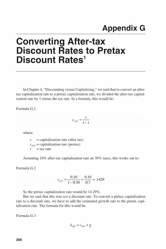
300
Appendix G
Converting After-tax Discount Rates to PretaxDiscount Rates1
In Chapter 4, “Discounting versus Capitalizing,” we said that to convert an after-tax capitalization rate to a pretax capitalization rate, we divided the after-tax capital-ization rate by 1 minus the tax rate. In a formula, this would be:
Formula G.1
where:
c = capitalization rate (after tax)c(pt) = capitalization rate (pretax)t = tax rate
Assuming 10% after-tax capitalization rate an 30% taxes, this works out to:
Formula G.2
So the pretax capitalization rate would be 14.29%.But we said that this was not a discount rate. To convert a pretax capitalization
rate to a discount rate, we have to add the estimated growth rate to the pretax capi-talization rate. The formula for this would be:
Formula G.3
k(pt) = c(pt) + g
c pt( )
.
– .
.
..= = =0 10
1 0 30
0 10
0 71429
cc
tpt( ) =−1
3953 P-29 8/29/02 2:30 PM Page 300
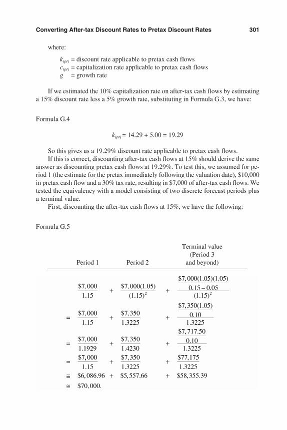
where:
k(pt) = discount rate applicable to pretax cash flowsc(pt) = capitalization rate applicable to pretax cash flowsg = growth rate
If we estimated the 10% capitalization rate on after-tax cash flows by estimatinga 15% discount rate less a 5% growth rate, substituting in Formula G.3, we have:
Formula G.4
k(pt) = 14.29 + 5.00 = 19.29
So this gives us a 19.29% discount rate applicable to pretax cash flows.If this is correct, discounting after-tax cash flows at 15% should derive the same
answer as discounting pretax cash flows at 19.29%. To test this, we assumed for pe-riod 1 (the estimate for the pretax immediately following the valuation date), $10,000in pretax cash flow and a 30% tax rate, resulting in $7,000 of after-tax cash flows. Wetested the equivalency with a model consisting of two discrete forecast periods plusa terminal value.
First, discounting the after-tax cash flows at 15%, we have the following:
Formula G.5
Terminal value(Period 3
Period 1 Period 2 and beyond)
$ ,
.
$ , ( . )
( . )
$ , ( . )( . )
. – .( . )
$ ,
.
$ ,
.
$ , ( . )
..
$ ,
.
$ ,
.
$ , .
..
$
7 000
1 15
7 000 1 05
1 15
7 000 1 05 1 05
0 15 0 051 15
7 000
1 15
7 350
1 3225
7 350 1 05
0 101 3225
7 000
1 1929
7 350
1 4230
7 717 50
0 101 3225
7
2 2+ +
= + +
= + +
= ,,
.
$ ,
.
$ ,
.$ , . $ , . $ , .
$ , .
000
1 15
7 350
1 3225
77 175
1 32256 086 96 5 557 66 58 355 39
70 000
+ +
≅ + +≅
Converting After-tax Discount Rates to Pretax Discount Rates 301
3953 P-29 8/29/02 2:30 PM Page 301
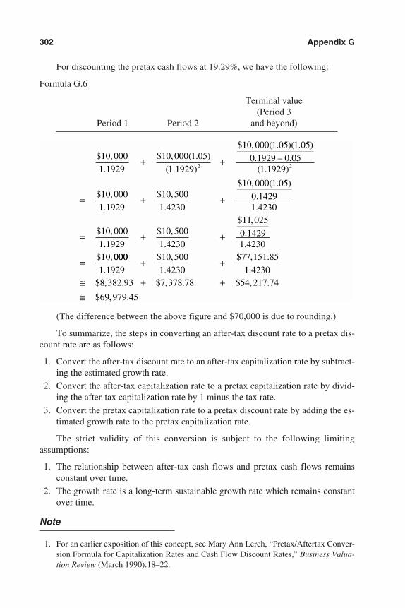
For discounting the pretax cash flows at 19.29%, we have the following:
Formula G.6
Terminal value(Period 3
Period 1 Period 2 and beyond)
(The difference between the above figure and $70,000 is due to rounding.)
To summarize, the steps in converting an after-tax discount rate to a pretax dis-count rate are as follows:
1. Convert the after-tax discount rate to an after-tax capitalization rate by subtract-ing the estimated growth rate.
2. Convert the after-tax capitalization rate to a pretax capitalization rate by divid-ing the after-tax capitalization rate by 1 minus the tax rate.
3. Convert the pretax capitalization rate to a pretax discount rate by adding the es-timated growth rate to the pretax capitalization rate.
The strict validity of this conversion is subject to the following limitingassumptions:
1. The relationship between after-tax cash flows and pretax cash flows remainsconstant over time.
2. The growth rate is a long-term sustainable growth rate which remains constantover time.
Note
1. For an earlier exposition of this concept, see Mary Ann Lerch, “Pretax/Aftertax Conver-sion Formula for Capitalization Rates and Cash Flow Discount Rates,” Business Valua-tion Review (March 1990):18–22.
$ ,
.
$ , ( . )
( . )
$ , ( . )( . )
. – .( . )
$ ,
.
$ ,
.
$ , ( . )
.
.
$ ,
.
$ ,
.
$ ,
.
.$ ,
10 000
1 1929
10 000 1 05
1 1929
10 000 1 05 1 05
0 1929 0 051 1929
10 000
1 1929
10 500
1 4230
10 000 1 05
0 14291 4230
10 000
1 1929
10 500
1 4230
11 025
0 14291 4230
10
2 2+ +
= + +
= + +
= 000000
1 1929
10 500
1 4230
77 151 85
1 42308 382 93 7 378 78 54 217 74
69 979 45
.
$ ,
.
$ , .
.$ , . $ , . $ , .
$ , .
+ +
≅ + +≅
302 Appendix G
3953 P-29 8/29/02 2:30 PM Page 302
303
Cost of Capital
Estimation and ApplicationsSecond Edition
CPE SELF-STUDY EXAMINATION
About the CPE Self-study Examination
Prerequisites: NoneRecommended CPE credits: 8 HoursKnowledge level: BasicArea of study: Management/Consulting Services
The credit hours recommended are in accordance with the AICPA Standards forCPE programs. Since CPE requirements are set by each state, you need to check withyour State Board of Accountancy concerning required CPE hours and fields of study.
If you decide to take this CPE examination, follow the directions below. This ex-amination fee is $59. Means of payment are shown on the answer form.
The CPE examination is graded no later than two weeks after receipt. The pass-ing score is at least 70%. John Wiley & Sons, Inc. will issue a certificate of comple-tion to successful participants to recognize their achievement.*
Photocopy one copy of the answer sheet for each additional participant whowishes to take the CPE examination. Each participant should complete the answer formand return it with the $59 fee.
The enclosed CPE examination will expire on December 31, 2004. Completedexams must be postmarked by that date.
Registered with the National Association of State Boards of Accountancy as a sponsor ofcontinuity professional education on the National Registry of CPE Sponsors. State boards ofaccountancy have final authority on the acceptance of individual courses. Complaints regardingregistered sponsors may be addressed to NASBA, 150 Fourth Avenue North, Suite 700,Nashville, TN 37219-2417; (615) 880-4200; fax (615) 880-4292.
3953 P-30 8/29/02 2:30 PM Page 303

Directions for the CPE Course
Complete the examination after reading all chapters in Cost of Capital, Estima-tion and Applications, Second Edition. Record your answers by writing a letter (a–e),true, or false on the line for that question on the answer form. Upon completion of theexamination, cut out the answer sheet, enclose it in a stamped envelope, and mail tothe following address:
CPE DirectorJohn Wiley & Sons, Inc.7222 Commerce Ctr. DriveSuite 240Colorado Springs, CO 80919
304 Cost of Capital
3953 P-30 8/29/02 2:30 PM Page 304

COST OF CAPITAL: ESTIMATION AND APPLICATIONS Second Edition
CPE Examination
Record your CPE answers on the answer form provided below and return this pagefor grading.
Mail to:CPE Director
John Wiley & Sons, Inc., 7222 Commerce Center Drive, Suite 240, Colorado Springs,CO 80919
Cost of Capital 305
PAYMENT OPTIONS□ Payment enclosed ($59.00).
(Make checks payable to JohnWiley & Sons, Inc.)Please add appropriate sales tax.Be sure to sign your order below.
Charge my:□ American Express□ Master Card□ Visa
Account number ______________
Expiration date _______________Please sign below for all creditcard orders.
Signature ________________________
NAME __________________________
FIRM NAME _____________________
ADDRESS _______________________
————————————————–
PHONE ( ) _____________________
CPA STATE LICENSE # ___________
SEE THE OTHER SIDE OF THIS PAGE FOR THE CPE FEEDBACK FORM
CPE ANSWERS
1. ____ 2. ____ 3. ____ 4. ____ 5. ____ 6. ____ 7. ____ 8. ____ 9. ____ 10. ____11. ____ 12. ____ 13. ____ 14. ____ 15. ____ 16. ____ 17. ____ 18. ____ 19. ____ 20. ____21. ____ 22. ____ 23. ____ 24. ____ 25. ____ 26. ____ 27. ____ 28. ____ 29. ____ 30. ____31. ____ 32. ____ 33. ____ 34. ____ 35. ____ 36. ____ 37. ____ 38. ____ 39. ____ 40. ____
CPE Exam ISBN: 0-471-26995-6
3953 P-30 8/29/02 2:30 PM Page 305

COST OF CAPITAL: ESTIMATION AND APPLICATIONS, Second Edition
CPE Feedback
1. Do you agree with the publisher’s determination of CPE credit hours?Yes ____ No ____
2. Was the content relevant? Yes ____ No ____
3. Was the content displayed clearly? Yes ____ No ____
4. Did the content enhance your professional competence? Yes ____ No ____
5. Was the content timely and effective? Yes ____ No ____
How can we make the examination/content better? If you have any suggestions,please summarize them in the space below. We will consider them in developing fu-ture examinations.
—————————————————————————————————–
—————————————————————————————————–
—————————————————————————————————–
—————————————————————————————————–
—————————————————————————————————–
—————————————————————————————————–
—————————————————————————————————–
—————————————————————————————————–
—————————————————————————————————–
—————————————————————————————————–
306 Cost of Capital
Copyright © 2002 John Wiley & Sons, Inc.All rights reserved.
3953 P-30 8/29/02 2:30 PM Page 306

CONTINUING PROFESSIONAL EDUCATION: SELF-STUDYEXAMINATION
Multiple Choice:
1. For which of the following balance sheet components can cost of capital bemeasured?
a. Common equity
b. Preferred equity
c. Long-term debt
d. All of the above
2. Which of the following terms are properly used interchangeably?
a. Discount rate, capitalization rate, and cost of capital
b. Discount rate and capitalization rate, but not cost of capital
c. Discount rate and cost of capital, but not capitalization rate
d. Capitalization rate and cost of capital, but not discount rate
3. What is the measure of economic income preferred by most analysts for the in-come approach to valuation?
a. Net income
b. Net cash flow
c. Pretax income
d. Gross cash flow
4. Given the following:
Sales $1,000
Cost of goods sold 600
Depreciation 50
Interest 30
Owners’ compensation 100
Other expenses 200
Pretax income 220
Taxes 55
Net income 165
Capital expenditures 60
Additions to working capital 20
What is the net cash flow to invested capital?
a. $257.50
b. $177.50
Cost of Capital 307
3953 P-30 8/29/02 2:30 PM Page 307
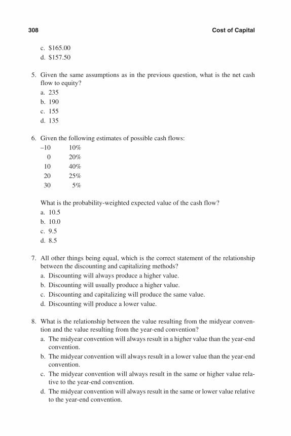
c. $165.00
d. $157.50
5. Given the same assumptions as in the previous question, what is the net cashflow to equity?
a. 235
b. 190
c. 155
d. 135
6. Given the following estimates of possible cash flows:
–10 10%
0 20%
10 40%
20 25%
30 5%
What is the probability-weighted expected value of the cash flow?
a. 10.5
b. 10.0
c. 9.5
d. 8.5
7. All other things being equal, which is the correct statement of the relationshipbetween the discounting and capitalizing methods?
a. Discounting will always produce a higher value.
b. Discounting will usually produce a higher value.
c. Discounting and capitalizing will produce the same value.
d. Discounting will produce a lower value.
8. What is the relationship between the value resulting from the midyear conven-tion and the value resulting from the year-end convention?
a. The midyear convention will always result in a higher value than the year-endconvention.
b. The midyear convention will always result in a lower value than the year-endconvention.
c. The midyear convention will always result in the same or higher value rela-tive to the year-end convention.
d. The midyear convention will always result in the same or lower value relativeto the year-end convention.
308 Cost of Capital
3953 P-30 8/29/02 2:30 PM Page 308
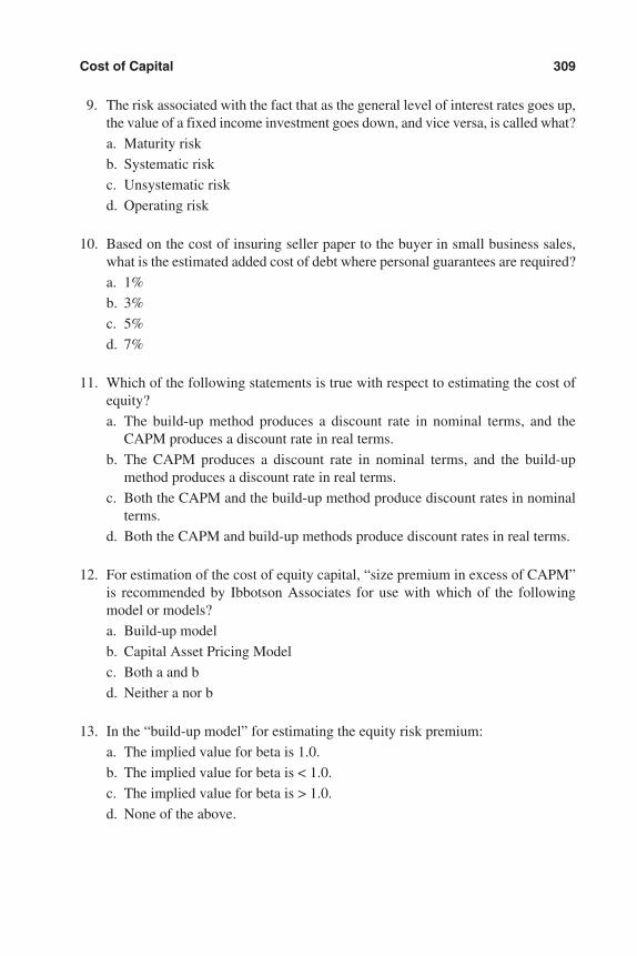
9. The risk associated with the fact that as the general level of interest rates goes up,the value of a fixed income investment goes down, and vice versa, is called what?
a. Maturity risk
b. Systematic risk
c. Unsystematic risk
d. Operating risk
10. Based on the cost of insuring seller paper to the buyer in small business sales,what is the estimated added cost of debt where personal guarantees are required?
a. 1%
b. 3%
c. 5%
d. 7%
11. Which of the following statements is true with respect to estimating the cost ofequity?
a. The build-up method produces a discount rate in nominal terms, and theCAPM produces a discount rate in real terms.
b. The CAPM produces a discount rate in nominal terms, and the build-upmethod produces a discount rate in real terms.
c. Both the CAPM and the build-up method produce discount rates in nominalterms.
d. Both the CAPM and build-up methods produce discount rates in real terms.
12. For estimation of the cost of equity capital, “size premium in excess of CAPM”is recommended by Ibbotson Associates for use with which of the followingmodel or models?
a. Build-up model
b. Capital Asset Pricing Model
c. Both a and b
d. Neither a nor b
13. In the “build-up model” for estimating the equity risk premium:
a. The implied value for beta is 1.0.
b. The implied value for beta is < 1.0.
c. The implied value for beta is > 1.0.
d. None of the above.
Cost of Capital 309
3953 P-30 8/29/02 2:30 PM Page 309
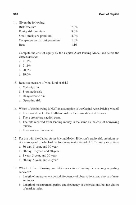
14. Given the following:
Risk-free rate 7.0%
Equity risk premium 8.0%
Small stock size premium 4.0%
Company-specific risk premium 1.0%
Beta 1.10
Compute the cost of equity by the Capital Asset Pricing Model and select thecorrect answer:
a. 21.2%
b. 21.1%
c. 20.8%
d. 19.0%
15. Beta is a measure of what kind of risk?
a. Maturity risk
b. Systematic risk
c. Unsystematic risk
d. Operating risk
16. Which of the following is NOT an assumption of the Capital Asset Pricing Model?
a. Investors do not reflect inflation risk in their investment decisions.
b. There are no transaction costs.
c. The rate received from lending money is the same as the cost of borrowingmoney.
d. Investors are risk averse.
17. For use with the Capital Asset Pricing Model, Ibbotson’s equity risk premium se-ries correspond to which of the following maturities of U.S. Treasury securities?
a. 30-day, 5-year, and 30-year
b. 30-day, 10-year, and 20-year
c. 1 year, 5-year, and 20-year
d. 30-day, 5-year, and 20-year
18. Which of the following are differences in estimating beta among reportingservices?
a. Length of measurement period, frequency of observations, and choice of mar-ket index
b. Length of measurement period and frequency of observations, but not choiceof market index
310 Cost of Capital
3953 P-30 8/29/02 2:30 PM Page 310
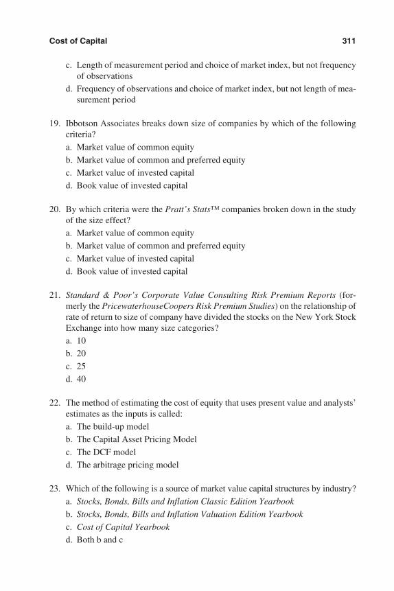
c. Length of measurement period and choice of market index, but not frequencyof observations
d. Frequency of observations and choice of market index, but not length of mea-surement period
19. Ibbotson Associates breaks down size of companies by which of the followingcriteria?
a. Market value of common equity
b. Market value of common and preferred equity
c. Market value of invested capital
d. Book value of invested capital
20. By which criteria were the Pratt’s Stats™ companies broken down in the studyof the size effect?
a. Market value of common equity
b. Market value of common and preferred equity
c. Market value of invested capital
d. Book value of invested capital
21. Standard & Poor’s Corporate Value Consulting Risk Premium Reports (for-merly the PricewaterhouseCoopers Risk Premium Studies) on the relationship ofrate of return to size of company have divided the stocks on the New York StockExchange into how many size categories?
a. 10
b. 20
c. 25
d. 40
22. The method of estimating the cost of equity that uses present value and analysts’estimates as the inputs is called:
a. The build-up model
b. The Capital Asset Pricing Model
c. The DCF model
d. The arbitrage pricing model
23. Which of the following is a source of market value capital structures by industry?
a. Stocks, Bonds, Bills and Inflation Classic Edition Yearbook
b. Stocks, Bonds, Bills and Inflation Valuation Edition Yearbook
c. Cost of Capital Yearbook
d. Both b and c
Cost of Capital 311
3953 P-30 8/29/02 2:30 PM Page 311
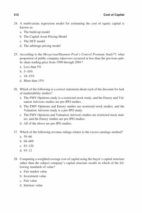
24. A multivariate regression model for estimating the cost of equity capital isknown as:
a. The build-up model
b. The Capital Asset Pricing Model
c. The DCF model
d. The arbitrage pricing model
25. According to the Mergerstat/Shannon Pratt’s Control Premium Study™, whatproportion of public company takeovers occurred at less than the previous pub-lic share trading price from 1998 through 2001?
a. Less than 5%
b. 5–10%
c. 10–15%
d. More than 15%
26. Which of the following is a correct statement about each of the discount for lackof marketability studies?
a. The FMV Opinions study is a restricted stock study, and the Emory and Val-uation Advisors studies are pre-IPO studies.
b. The FMV Opinions and Emory studies are restricted stock studies, and theValuation Advisors study is a pre-IPO study.
c. The FMV Opinions and Valuation Advisors studies are restricted stock stud-ies, and the Emory studies are pre-IPO studies.
d. All of the above are pre-IPO studies.
27. Which of the following revenue rulings relates to the excess earnings method?
a. 59–60
b. 68–609
c. 83–120
d. 93–12
28. Computing a weighted average cost of capital using the buyer’s capital structurerather than the subject company’s capital structure results in which of the fol-lowing standards of value?
a. Fair market value
b. Investment value
c. Fair value
d. Intrinsic value
312 Cost of Capital
3953 P-30 8/29/02 2:30 PM Page 312
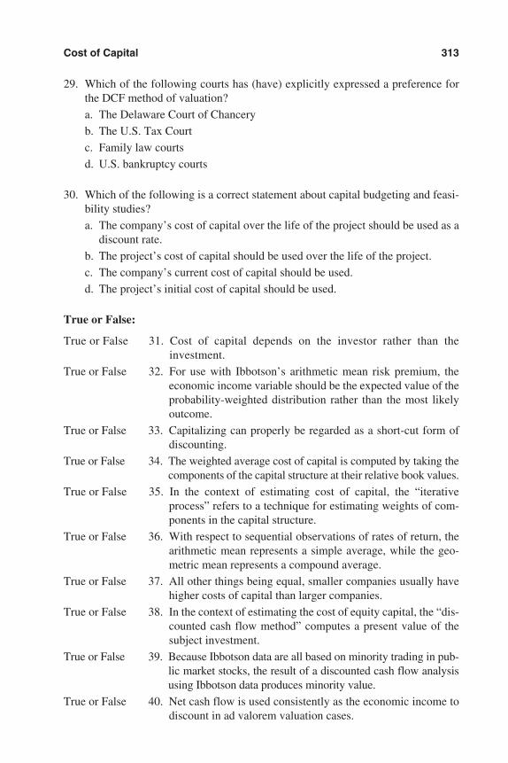
29. Which of the following courts has (have) explicitly expressed a preference forthe DCF method of valuation?
a. The Delaware Court of Chancery
b. The U.S. Tax Court
c. Family law courts
d. U.S. bankruptcy courts
30. Which of the following is a correct statement about capital budgeting and feasi-bility studies?
a. The company’s cost of capital over the life of the project should be used as adiscount rate.
b. The project’s cost of capital should be used over the life of the project.
c. The company’s current cost of capital should be used.
d. The project’s initial cost of capital should be used.
True or False:
True or False 31. Cost of capital depends on the investor rather than theinvestment.
True or False 32. For use with Ibbotson’s arithmetic mean risk premium, theeconomic income variable should be the expected value of theprobability-weighted distribution rather than the most likelyoutcome.
True or False 33. Capitalizing can properly be regarded as a short-cut form ofdiscounting.
True or False 34. The weighted average cost of capital is computed by taking thecomponents of the capital structure at their relative book values.
True or False 35. In the context of estimating cost of capital, the “iterativeprocess” refers to a technique for estimating weights of com-ponents in the capital structure.
True or False 36. With respect to sequential observations of rates of return, thearithmetic mean represents a simple average, while the geo-metric mean represents a compound average.
True or False 37. All other things being equal, smaller companies usually havehigher costs of capital than larger companies.
True or False 38. In the context of estimating the cost of equity capital, the “dis-counted cash flow method” computes a present value of thesubject investment.
True or False 39. Because Ibbotson data are all based on minority trading in pub-lic market stocks, the result of a discounted cash flow analysisusing Ibbotson data produces minority value.
True or False 40. Net cash flow is used consistently as the economic income todiscount in ad valorem valuation cases.
Cost of Capital 313
3953 P-30 8/29/02 2:30 PM Page 313
314
Index
Ad valorem taxation, 207–223Adams, Estate of, v. Commissioner,
187n. 1, 197Adjusted beta, see betaAdjusted present value (APV)
and capital budgeting, 225, 227Alcar Group, The
and arbitrage pricing theory, 146American Depository Receipts
(ADRs)exclusion from size effect studies,
94American Institute of Certified
Public Accountants (AICPA)courses, 252
American Society of Appraisers(ASA)
Business Valuation Committee,63
Business Valuation Standardsdefinitions, 264–265
courses, 252American Stock Exchange (AMEX)
and long-term returns in excess ofCAPM, 87, 124
and SBBI Valuation EditionYearbook, 122, 127
and size effect data, 91–92as market measure in estimating
beta, 83in build-up model example, 67
Annin, Michaeland SBBI Valuation Edition
Yearbook, 117Arbitrage pricing theory (APT)
compared to CAPM, 143explanation of model, 143–144formula, 144multifactor approach, 43risk factors, 145–146
Arithmetic average equity riskpremium, 61
versus geometric average riskpremium, 120
Arithmetic average return, 92and calculation of equity risk
premium, 119Arithmetic mean
arithmetic mean return, 92formula for, 62versus geometric mean, 61–63
Assetstotal assets as measure of size, 94,
140
Baird & Co., see Emory pre-IPOstudies
Bajaj, Mukesh, 170n. 2Bankruptcy, 198–202Barad, Michael W., 66n. 4
using Ibbotson Associates data,116–142
Base period, 25Becker, Brian, 63n. 3Best-fit line
in measuring beta, 80–81Beta Book, 82, 83, 117, 134–138
1997 edition methodology, 86description of, 255explanation of lag effect and sum
beta, 87sample data, 136–137
Beta, 80–88and economic value added, 229and risk-free rate, 70and small company stocks, 75and standard errors, 86annual versus monthly betas, 125as measure of systematic risk, 36,
70, 124Beta Book and, 134–138CAPM v. build-up model, 68,
118, 265–266company-specific betas, 134, 138Cost of Capital Center and,
139–140differences in estimation, 82–83estimating expected rate of return,
72–75estimation of generally, 80–82,
135example of calculation of beta, 81Full Information Beta procedure,
138Ibbotson (adjusted) beta, 86–87,
135, 138in ad valorem taxation, 223lag effect, 86levered, unlevered, and relevered,
83–86, 135, 274–290modified (shrunk and lagged),
86–87
negative, 74peer group beta, 138proxy beta for private company,
70–71, 82SBBI Valuation Edition Yearbook
and, 87, 117sum beta versus ordinary least
squares beta, 87, 125tendency toward industry average
beta, 86, 118, 138U.S. Tax Court guidance, 195
Beta-adjusted size premia, see sizeeffect
BIRR Portfolio Analysis, Inc.and arbitrage pricing model
inputs, 146, 258BIZCOMPS®, 261Bloomberg
and foreign bond rates, 58Book value of equity
as measure of size, 93, 140Brealey, Richard A., 5, 10
and capital budgeting, 224and utility rate setting, 112n. 1on CAPM, 72n. 2on tax rates, 41n. 2, 63
Brinson, Gary P.and arbitrage pricing model, 144
Build-up models, 20, 57–69alternative model formula, 66and company-specific risk
premium, 67and ex post and ex ante risk
premia, 221–222estimating capitalization rate with,
181example of, 67–68for estimating cost of equity
capital, 37, 42formula for cost of equity capital,
58in U.S. Tax Court, 196–197use of beta-adjusted size premia
in, 123use of industry premia in, 118,
125–126use of S&P Corporate Value
Consulting data with, 99use of size effect data, 92
Business riskand economic value added, 229
3953 P-31 REV 8/29/02 2:30 PM Page 314
and levered betas, 83in arbitrage pricing model,
144–146Business Valuation Data,
Publications & InternetDirectory
as source of industry forecasts, 115Business Valuation Resources, LLC,
157Business Valuation Review, 63BVLibrary.comsm, 263BVMarketData.comsm, 107
and Mergerstat/Shannon Pratt’sControl Premium Study™,155n. 4
and The FMV Restricted StockStudy™, 166
and Valuation Advisors’ Lack ofMarketability DiscountStudy™, 169
Canadian Risk Premia over TimeReport, 140
Capital Asset Pricing Model(CAPM), 20, 70–78
adjusted (Mercer’s) CAPM, 265adjustment of leverage, 84an iterative process, 274–290and economic value added, 229and ex post and ex ante risk
premia, 221–222Beta Book calculations and,
134–135company-specific risk premium
in, 67compared to arbitrage pricing
model, 143–144compared to build-up model,
265–266Cost of Capital Yearbook and,
129, 132estimating cost of equity capital
with, 37, 42expanded CAPM formula, 76–77in Delaware courts, 194in U.S. Tax Court, 195–197incorporating size premium and
specific risk, 75–76S&P Corporate Value Consulting
data and, 99systematic risk, 36, 70–71underlying assumptions, 77–78use of beta-adjusted size premia
in, 123use of size effect data in, 92ValuSource PRO software and,
265–268Capital budgeting, 224–228, 232
capital investment projectselection, 9
evaluation of projects, 185Capital gain
as component of return oninvestment, 60
in measuring beta, 80
Capital investment project selection,see capital budgeting
Capital lossas component of return on
investment, 60in measuring beta, 80
Capital market dataand DCF method, 110source of data and commentary,
117Capital market theory (CMT), 71
and U.S. Tax Court, 194Capital structure risk, see financial
riskCapital structure
ability to change, 84actual versus hypothetical, 52and levered betas, 83book value versus market-
weighted structure, 223components of, 39–43industry-average capital structure,
52, 66, 201internally inconsistent projections,
190ratios and Cost of Capital Center,
139–140ratios and Cost of Capital
Yearbook, 128target capital structure and capital
budgeting, 227Capitalization formula, 22Capitalization rate
converting after-tax rate to pretaxrate, 32, 300–302
definition of, 12,development with ValuSourc
PRO software, 264–265discount rate distinguished, 7, 12,
21, 185factoring in marketability
discount, 165, 173relationship to discount rate, 23SBBI Valuation Edition Yearbook
and, 117weighted average excess earnings
capitalization rate, 181Capitalizing, 21
and minority versus controlvaluations, 153
combined with discounting, 27distinguished from discounting,
25excess earnings method as form
of, 178in computing WACC, 49problem with, 27
Cash bonus planand economic value added,
234–235Cash flows
adjustments to projected cashflows, 128
constant and perpetual, 210controlling interest and, 153, 156
growth forecasts, 133Ibbotson’s definition, 114incremental, 13nature of and level of value, 151net cash flows as measure of
economic income, 224, 225probability-weighted, 17tax-affecting, 126–127U.S. Tax Court concerns, 194yield in single-stage DCF model,
112Cassiere, George G., 63n. 3Center for Advanced Valuation
Studies (CAVS) courses, 253Chen, Peng
equity risk premium research, 78Chew, Donald
on economic value added,229–238
City of Chicago Commissioner ofConsumer Services, 204
Collapse of the Soviet Unionas unusual economic event, 120
Colonial Realty Co., In re, 201n. 31
Columbia Financial Advisorsrestricted stock studies, 167
Common errors, 184–192Common stock
as component of capital structure,39, 42–43
in computing WACC, 47Company risk, see unsystematic riskCompany-specific data
company analysis at Cost ofCapital Center, 139–140
for DCF cost of capital analysis,115
Company-specific risk premiumadjusted (Mercer’s) CAPM and,
266–268as subcomponent of risk
premium, 57factors to consider, 65in build-up model, 58, 67, 124incorporated into CAPM, 75–76to account for industry risk, 125
Comparable companiesuse of beta from, 118
Competitionand company-specific risk
premium, 67CompuServe, 255Confidence risk
and arbitrage pricing model, 145Consensus value, see fair market
valueConstant growth model
and DCF method, 110Control premium, 153
when to apply, 155–157Controlling interest, 52
and marketability discounts,172–173
prerogatives of control, 154
Index 315
3953 P-31 REV 8/29/02 2:30 PM Page 315
Controlling interest (Cont.)versus minority implications of
cost of capital data, 151–164versus minority interest in
Ibbotson data, 127–128Convertible preferred stock, 42Copeland, Tom, 4n. 4, 63
and arbitrage pricing model, 44n. 3
and choice of corporate decisionmodel, 225–226
Cost approachin ad valorem taxation, 208
Cost of Capital Center, 139–142description of, 255
Cost of Capital Quarterly (CCQ),see Cost of Capital Yearbook
Cost of Capital Yearbook, 52,128–134
data for DCF method, 64description of, 255formerly Cost of Capital
Quarterly, 117multistage DCF models and, 114single-stage DCF model and,
111–112use of NYSE index in
calculations, 83Cost of capital
applications, 9before-tax, 214Cost of Capital Yearbook and,
128, 129divisional, 13embedded versus market, 11Ibbotson workshops, 117impact of risk on, 36–37other terms for, 7project versus company, 224role in economic value added,
229–238SBBI Valuation Edition Yearbook
and, 117Cost of conventional debt, 37
after-tax, 212before-tax, 214in computing WACC, 47
Cost of equity capitaland the iterative process, 274–290as discount rate, 17Cost of Capital Center and,
139–140Cost of Capital Yearbook and,
128, 129estimating, 37tax effect, 212, 214–216using build-up model to estimate,
118using CAPM to estimate, 70–71,
118using DCF method to estimate,
109–115using Fama-French three-factor
model to estimate, 118Cost of preferred equity capital, 37
after-tax, 212Country-specific risk premium, 57Creating Shareholder Value, 10Currency-related risk, 58Customer base
and company-specific riskpremium, 67
Damagesrecovery of lost capital, 202–203
Damodaran, Aswath, 4n. 3Data measurement
frequency used to calculate beta,82
Debtas component of capital structure,
39, 40–41convertible, 42cost of conventional debt, 37long-term liabilities, 40personal guarantee, 41rating criteria, 40short-term interest-bearing debt, 40tax effect, 40–41
Decile groupsand size effect data, 90choice of, 125deciles 10a and 10b, 122
Definition of value, see standard ofvalue
Delaware courtsChancery Court, 193Supreme Court, 193
Delistingeffect on rates of return, 95
Dimensional Fund Advisors (DFA)Small Company 9/10 Fund
and size effect, 91–92Discount for lack of liquidity, see
marketability discountDiscount for lack of marketability,
see marketability discountDiscount rate, 6
adjusting for unsystematic risk, 76capitalization rate distinguished,
7, 12, 21, 185converting after-tax rate to pretax
rate, 32, 300–302DCF model formula, 110definition of, 10factoring in marketability
discount, 165, 173other terms for, 7relationship to capitalization rate,
23SBBI Valuation Edition Yearbook
and, 117smallest companies, 65tax effect, 126–127U.S. Tax Court concerns, 194
Discounted cash flow (DCF)method, 37
ad valorem taxation, 207, 222bankruptcy cases, 201–202capital budgeting, 225–227, 232
Cost of Capital Yearbook and,133–134
family law cases, 197–198for estimating cost of capital,
109–115for estimating equity risk
premiums, 64in Delaware courts, 193–194in the U.S. Tax Court, 194–197industry statistics for, 129multistage models described,
113–114public versus private companies,
110single-stage and multistage
models, 42single-stage model described,
110–113tax effect, 126–127utility rate-setting, 203–204
Discountingcombined with capitalizing, 27distinguished from capitalizing, 25in computing WACC, 49minority versus control valuations,
153problem with, 27
Discrete projection period, 28Distributions, see dividendsDividends
as cash flow yield in DCF model,112
as component of rate of return, 42as component of return on
investment, 60as proxy for market yield, 41in calculation of ex ante risk
premium, 222in measuring beta, 80in single-stage DCF model, 134
Divisional cost of capital, 13Done Deals Data, 261DoneDeals Complete Transaction
Handbook 2000-2001, 262Dow Jones Industrial Average
and equity risk premium, 119
Earnings before depreciation,interest and taxes (EBDIT)
in ad valorem taxation, 209Earnings before interest (EBI),
216–217Earnings before interest and taxes
(EBIT), 19Earnings before interest, taxes,
depreciation, and amortization(EBITDA)
distinguished from free cash flow,16
five-year average as measure ofsize, 94, 140
Economic income measurechoice of in income approach,
186–188Economic profit, 5
316 Index
3953 P-31 REV 8/29/02 2:30 PM Page 316
Economic value added (EVA), 5and capital budgeting, 224role of cost of capital in, 229–238
Electronic Data Gathering, Analysis,and Retrieval (EDGAR)Service, 259
Emory pre-IPO studies, 168–170Employees
number of as measure of size, 94,140
Equityvaluing, 16
Equity risk premium (ERP), 60–61ad valorem taxation, 221arithmetic average equity risk
premium, 61as subcomponent of risk
premium, 57definition of, 118–119historical data for, 61, 117in build-up model example, 67long-horizon premium, 132recent research, 78SBBI Valuation Edition Yearbook
and, 118size effect and, 90using DCF method for, 64
European Economic Communitydevelopment of as unusual
economic event, 120Ex post and ex ante risk premia,
221–223Excess earnings method
conceptual basis, 178reasonableness check, 188-189relationship to cost of capital,
176–183steps in applying, 178–179unrealistic cost of capital and,
188–189Excess return
as equity risk premium, 61size effect and, 90used in measuring beta, 80
Exhibits, list of, xvii–xviiiExpected returns, 34
Fair market value, 52, 151, 155Fair value, 193Falaschetti, Dominic
and SBBI Valuation EditionYearbook, 117
Fama, Eugene, 132on equity risk premium, 78
Fama-French three-factor model, 87
Cost of Capital Yearbook and,132–133
formula, 133, and Beta Bookcalculations, 134
in Beta Book, 117Family law, 197–198Feasibility studies, 224–228Federal Communications
Commission (FCC), 203–204
Federal Energy RegulatoryCommission (FERC), 204
Federal Power Comm’n v. HopeNatural Gas Co., 203n. 34, 204n. 35
Federal Reserve BankSt. Louis branch, 60
Financial buyer, 156Financial companies
exclusion from size effect studies,94
Financial management systemdefinition of, 232reengineering with economic
value added, 232–233Financial press
and yield-rate data, 60Financial reporting services
and published betas, 82Financial risk
and levered betas, 83Firm size premium, see size effectFirst Call database, 257Flotation costs
as value adjustment, 220–221FMV Opinions, Inc., 166FMV Restricted Stock Study™, The,
166–168Formal valuation report
footnoting sources, 68Formulas
as used for capital budgeting,225–226
Fowler, Bradley A., 172n. 3Free cash flow, 9, 15
distinguished from EBITDA, 16,see also net cash flow
Freeman, Estate of, v.Commissioner, 195n. 7
French, Kenneth, 132on equity risk premium, 78
Full Information Beta procedure, seebeta
Gelman, Miltonrestricted stock study, 167
General Motors Acceptance Corp.versus Jones, 199n. 24
Generally accepted accountingprinciples (GAAP), 178
and economic value added, 230Geometric average risk premium
versus arithmetic average riskpremium, 120
Geometric meanformula for, 62versus arithmetic mean, 61–63
Global analysisat Cost of Capital Center, 139–140
Glossary of terms, 292–299Glueck, In re,200n. 28Going concern value versus
liquidation value, 230Gold-mining companies
and beta, 74
Goodwilland excess earnings method, 176
Gordan, Myron Jand DCF method, 133
Gordon Growth Model, 25–27ad valorem taxation, 222Cost of Capital Yearbook and, 134DCF method and, 110formula for, 134in estimating equity risk
premiums, 64utility rate-setting, 204
Grabowski, Rogerpremiums over CAPM, 99S&P CVC Risk Premium Report,
140size effect research, 93use of data with ValuSource PRO
software, 265, 268Gray, Ian, 63n. 3Green Tree Fin. Serv. Corp. v.
Smithwick, 199n. 25Grimes v. Vitalink Comm. Corp.,
193n. 2Gross v. Commissioner, 18
n. 1, 196n. 11, 197Growth estimates, 64
and DCF method, 110unrealistic projections, 189
Growth ratead valorem taxation, 215–218as growth stages in multistage
DCF models, 113–114converting after-tax capitalization
rate to pretax rate, 32, 300–302Cost of Capital Center and,
139–140Cost of Capital Yearbook and,
128, 133–134expected, 7, 26in calculation of ex ante risk
premium, 222in single-stage DCF model,
112–113long-term, 23perpetual annual growth rate,
112projected, 49
Guide to Business Valuations, 178Guideline companies
adjustment of leverage inestimating beta, 83
Guiffre v. Baker, 198n. 21
Hardzog, In re, 199Heck, Estate of, v. Commissioner,
187n. 1, 197Hendrickson, Estate of, v.
Commissioner, 195n. 8–10High-financial-risk portfolio, 94High-tech companies
and beta, 73Historical data
for equity risk premium, 61market data, 117
Index 317
3953 P-31 REV 8/29/02 2:30 PM Page 317

Historical time period forcalculations, 63–64
exponential weighting of tocalculate the equity riskpremium, 121
recent versus long-term history, 63standard error and, 63
Hoemke, Carl R. E.on ad valorem taxation, 207–223
Horizon risk, see maturity riskHurdle rate, 5, 13Hybrid securities, 42–43
I/B/E/S database, 112, 257and long-term growth rate
estimates, 133IBA Market Data Base, 262Ibbotson, Roger G., 3
arbitrage pricing model, 144early market data, 120equity risk premium research, 78establishment of Ibbotson
Associates, 116on minority versus control impact
on cost of capital, 153study of long-term market
analysis, 117sum beta, 87n. 4
Ibbotson.com, 139Ibbotson’s Small Company Stock
series, 122Ibbottson Associates, 5, 255–256
calculation of equity riskpremium, 119
Cost of Capital Center, 99cost of capital workshops, 117data for equity discount rate, 20,
59–60data for equity risk premium,
61–64data for industry-average capital
structure, 52firm size phenomenon, 75industry risk adjustment factors,
65measurement period for beta, 82size effect data, 90–93use of data with ValuSource PRO
software, 265–268use of excess returns in measuring
beta, 80using Ibbotson data, 116–142
Incentive compensation, 233–234Income adjustmentslinear versus multiplicative, 210–218Income approach
ad valorem taxation, 208–209adjustments for minority or
controlling interests, 128, 153bankruptcy cases, 201–202choice of economic income
measure, 186–188cost of capital analysis, 118critical data for, 128–129use of capitalization rate, 21
Income streamand excess earnings method, 178definition of for ad valorem
taxation, 209Industry adjustment factor
in build-up model example, 67Industry outlook data, see industry
statisticsIndustry premium
compared to industry beta, 118formula for, 126in build-up model, 118, 126SBBI Valuation Edition Yearbook
and, 117, 125–126Industry risk
as factor in company-specific riskpremium, 65–66
build-up model, 58industry multiples and Cost of
Capital Center, 139–140problem of double-counting risk
factors, 125Industry statistics, 52
industry analysis at Cost ofCapital Center, 139–140
industry average price in DCFmethod, 110
industry outlook for DCF cost ofcapital analysis, 115
industry-level financial data, 128Inflation
as component of risk-free rate, 59as unusual economic event, 120inflation risk and arbitrage pricing
model, 144, 145uncertainty of, 60
Institute of Business Appraiserscourses, 253IBA Market Data Base, 262
Intangible assetsad valorem taxation, 207excess earnings method, 176, 178
Interest rate risk, see maturity riskInterest rates
using cost of capital to set inbankruptcy, 198–201
Internal rate of return (IRR)calculations
ad valorem taxation, 219–220Internal Revenue Service (IRS), 194International Business Brokers
Association (IBBA), 107International Cost of Capital
Perspectives Report, 140, 142International Cost of Capital
Report, 140, 141International Equity Risk Premia
Report, 139International investing, 57–58Intrinsic value, 156Invested capital, 16Investment bankers
use of DCF method by, 64Investment rate risk, see maturity riskInvestment value, 52, 151, 155
as reflecting synergies, 156Iterative process
adjusting capital structure toestimate beta, 84
computing WACC, 49example of, 274–290multistage DCF models, 114
Jaffe, Jeffrey F.and arbitrage pricing model,
143n. 1Johnson, Bruce
restricted stock study, 167Joyce, Allyn A., 63n. 3Julius, Michael, 265, 267–268
Kaltman, Todd A., 30n. 1Kaplan, Paul D., 63n. 3
Full Information Beta procedure,138
lag effect research, 86sum beta, 87n. 4
Kaufman, Mike, 3n. 1Key person
and company-specific riskpremium, 67
Key supplierand company-specific risk
premium, 67King, David
premiums over CAPM, 99S&P CVC Risk Premium Report,
140size effect research, 93use of data with ValuSource PRO
software, 265, 268Klauss, Estate of, v. Commissioner,
196n. 13–14Koller, Tim, 4n. 4, 63
arbitrage pricing model, 144n. 3Koopmans v. Farm Credit Serv.,
198n. 22
Lag effect, see betaLas Vegas Dodge, Inc. v. United
States, 195n. 5Lawsuits
and company-specific riskpremium, 67
Least squares regression beta, 87Lee, Mark
on relationship between stockmarket and M&A market,156–157
Lerch, Mary Ann, 32n. 2, 300n. 1Leuhrman, Timothy A.
and adjusted present value (APV)analysis, 227
Levels of valuechart, 151, 152synergistic value, 156
Leverageadjusting for beta estimation, 83as factor in company-specific risk
premium, 65, 66
318 Index
3953 P-31 REV 8/29/02 2:30 PM Page 318

Leveraged buyoutsand economic value added, 236
Leveraged stock optionsand economic value added, 234,
235–237Levered beta, see betaLinter, John
and CAPM, 129Liquidation value v. going concern
value, 230Long-term call option, see warrantLong-term market analysis, 117
M.G. Bancorp., Inc. v. LeBeau,194n. 4
M.P.M. Enter.,Inc. v. Gilbert, 194n. 3Macroeconomic forecasts
arbitrage pricing theory, 146long-term for DCF cost of capital
analysis, 115,Maggos, Estate of, v. Commissioner,
196n. 12Maher, Michael
restricted stock study, 167Mahoney, In re, 201n. 30Malkiel, Burton
on equity risk premium, 78Management Planning, Inc.
restricted stock study, 167Market approach
ad valorem taxation, 208comparable market data 128critical data for, 128–129in U.S. Tax Court, 194use of capitalization rate, 21
Market commentary, 117Market index
used to calculate beta, 82–83Market risk, see systematic riskMarket timing risk
arbitrage pricing model and, 146Market value of equity
as measure of size, 93, 140company-specific risk premium,
66the iterative process, 274–290
Market value of invested capital(MVIC)
as measure of size, 94, 140company-specific risk premium, 66in computing WACC, 49MVIC/EBITDA and MVIC/sales
multiples, 107procedure to determine, 46
Market valuestandard in ad valorem taxation,
208versus book value in WACC, 45
Market yieldand preferred equity, 41
Marketability discountbuilding into discount rate or
capitalization rate, 165, 173discrete percentage deduction,
165–172
in bankruptcy case, 202Quantitative Marketability
Discount Model, 173–174,271–272
Market-capitalization weightedindexes, 83, 91–92
Martin, Jr., Harold G.on the iterative process, 274–290
Matthews, Gilbert E.on expected growth and capital
expenditures, 189n. 2Mattson, Michael
and build-up model, 92Maturity risk, 35
and arbitrage pricing model, 143,145
as component of risk-free rate, 59use of Treasury-bill rate to avoid,
83see also risk
McDowell, Tarausing Ibbotson Associates data,
116–142Measurement period
length used to calculate beta, 82Mercer Capital, 173Mercer, Z. Christopher, 10n. 1
Quantitative MarketabilityDiscount Model, 173
ValuSource PRO software,264–272
Mergent, Inc., 37, 259as source of company data, 115
Merger Yearbook, The, 261Mergers & Acquisitions in Canada,
260Mergers & Acquisitions Quarterly,
260Mergers & Acquisitions Sourcebook,
260Mergers and acquisitions (M&A)
marketrelationship to stock market,
156–158Mergers and Acquisitions, The
Dealmaker’s Journal, 259Mergerstat Control Premium
Study™, 157Mergerstat Online Transaction
Roster 2001-2002, 259Mergerstat Review, 259Mergerstat/Shannon Pratt’s Control
Premium Study™, 153, 260negative control premiums in, 157sample data, 159–163
Merrill Lynch, 256Microcap stocks
publicly traded, 122, 125Midyear convention, 30–32
capitalization, 30discounting, 30
Minority interest, 52inability to affect capital structure,
84marketability discount data and, 166
versus control implications in costof capital data, 151–164
versus controlling interest inIbbotson data, 127–128
Modified beta, see betaMoody’s, see Mergent, Inc.Moroney, Robert
restricted stock study, 167Morton v. Commissioner, 195n. 6Multex-ACE, 258Multiple linear regression model, 132Murrin, Jack, 4n. 4, 63
arbitrage pricing model, 144n. 3Myers, Stewart C., 5, 10
capital budgeting, 224CAPM 72n. 2tax rates, 41n. 2, 63utility rate-setting, 112n. 1
Nasdaq Stock Marketin build-up model example, 67long-term returns in excess of
CAPM, 87, 124SBBI Valuation Edition Yearbook
and, 122, 127size effect data, 91–92, 94
National Association of CertifiedValuation Analysts’ courses, 253
Negative beta, see betaNet cash flow, 9
ad valorem taxation, 209computing WACC, 49defined, 15net cash flow to equity (NCFe), 16net cash flow to invested capital
(NCFf), 16net income as proxy for, 112reasons for preferring, 19–20single-stage DCF model, 112versus net income, 187–188
Net incomeapplying net cash flow discount
rate to, 187–188as proxy for net cash flows in
DCF model, 112five-year average as measure of
size, 93, 140Net operating income (NOI), 216–217Net operating profit
and economic value added, 229New York Stock Exchange (NYSE)
1-2 Indexbenchmark for calculating the
equity risk premium, 119New York Stock Exchange (NYSE)
Composite Index, 35, 36, 61as market measure in estimating
beta, 70, 83benchmark for calculating the
equity risk premium, 119calculation of ex ante risk
premium, 222capitalization ranking and size
effect, 91size categories, 93
Index 319
3953 P-31 REV 8/29/02 2:30 PM Page 319
New York Stock Exchange (NYSE)long-term returns in excess of
CAPM, 124SBBI Valuation Edition Yearbook
and, 122, 125, 127New York Times, The, 60Nonoperating holding companies
exclusion from size effect studies,94
Normalization adjustments, 26North American Industry
Classification System (NAICS)code, 157
Notation system, xxxi
Oglesby and Jones, In re, 199n. 26Operating margin
as measure of risk, 99Ordinary least squares beta, see betaOver-the-counter (OTC) index
as market measure in estimatingbeta, 83
size effect data, 91–92
Partnership interestas component of capital structure,
39, 42–43Partnership Spectrum, The, 262Peer group beta, see betaPersonal guarantee
as cost of debt, 41Peterson, James D.
Full Information Beta procedure,138
sum beta, 87n. 4Portfolio diversification
company-specific risk factor,75–76
unsystematic risk, 72Portfolio management theory, 71Portfolio managers
use of DCF method by, 64Portfolio rates of return, 95Pratt’s Stats™, 262
size effect, 90, 99, 105–107small companies, 65
Preferred stockand yield rate, 41as component of capital structure,
39, 41–42convertible, 42cost of capital for preferred
equity, 37in computing WACC, 47rating criteria, 42
Pre-initial public offering (IPO)studies, 167–172
Premium for risk, see risk premiumPrerogatives of control, 154Present value
capital budgeting, 224, 225, 227current stock price as, 109in determining cost of equity
capital, 64interest rates in bankruptcy, 198
relationship to required rate ofreturn, 36
total, 27Price/earnings ratios
and pre-IPO studies, 167PricewaterhouseCoopers Risk
Premium Study, 140PricewaterhouseCoopers studies, see
Standard & Poor’s CorporateValue Consulting Studies
Principles of Corporate Finance, 63on capital budgeting, 224
Privately held companiesDCF method, 110determining proxy beta for,
70–71, 82Property taxation, see ad valorem
taxationPublic offering registration
prerogative of control, 156Publicly traded companies
as source of cost of capital data,153
DCF method, 110implicit minority discount, 127marketability discount, 165microcap stocks, 122
Publicly traded price historyexclusion of companies lacking
from size effect studies, 94public trading price and takeovers,
157
Quantitative Marketability DiscountModel (QMDM), 173–174,271–272
Railroad companyad valorem taxation, 207
Rankin v. DeSarno, 198n. 23Rappaport, Alfred, 10Rate of return
arbitrage pricing model, 143current, 12data for size effect, 90economic value added, 224, 229estimating expected rate of return
with beta, 72–75excess returns over Treasury-bill
returns, 132expected by venture capitalists,
173expected, 34, 42, 58, 153historical versus expected, 185–186internal rate of return, 219–220portfolio rates of return, 95required, 7, 36risk, 34total, 10, 27use of DCF method to estimate
expected equity rate of return,110
Ratiosas used for capital budgeting,
225–226
Reasonableness check, 180with excess earnings method,
188–189Regression analysis
and size premiums, 95single versus multiple regression,
143Regulatory changes
and company-specific riskpremium, 67
Reilly, Frank K.arbitrage pricing model, 144n. 2
Relevered beta, see betaRental rate
as component of risk-free rate, 59Research and development (R&D)
and economic value added, 230Residual risk, see unsystematic riskResidual value, see terminal valueRestricted stock studies
and marketability discount,166–167
Return on earnings (ROE), 230Return on equity as measure of risk,
99Return on investment (ROI), 230Revenue Ruling 59-60, 194Revenue Ruling 68-609, 176–177,
182Risk Premia over Time Report, 140
description of, 255Risk premium, 34
arithmetic risk premium, 99Cost of Capital Center and,
139–140ex post and ex ante in ad valorem
taxation, 221–223subcomponents of, 57–58
Riskad valorem taxation and, 221–223business versus financial risk, 135currency-related, 58definition of, 34double-counting risk factors, 124eliminating unsystematic risk, 35impact on cost of capital, 36–37maturity risk, 35measures of from financial
statements, 99of the project, 13overall, 13premium for, 34, 57risk factors in arbitrage pricing
model, 143, 145–146risk index, 126systematic risk and CAPM, 36,
132, 143systematic risk, 35–36, 70–71,types of, 35unsystematic risk, 36
Risk-free rate, 34, 57–60calculation of ex ante risk
premium, 222CAPM, 79, 132components of, 59
320 Index
3953 P-31 REV 8/29/02 2:30 PM Page 320

cost of equity models, 118foreign country, 58in build-up model example, 67premiums over, 96–98risk-free investment in measuring
beta, 80selecting risk-free maturity, 60U.S. Treasury securities, 59, 119
Riskless rate, see risk-free rateRMA Annual Statement Studies, 52Roper, William
arbitrage pricing theory, 146Ross, Stephen A.
arbitrage pricing model, 143n. 1Rule 144
and restricted stock studies, 166
S corporationtax effect generally, 127tax-affecting and the U.S. Tax
Court, 187, 197Sales
as measure of size, 94, 140Sanity check, see reasonableness
checkSecurities and Exchange
Commission (SEC)filings as source of company data,
115initial public offering prospectus,
167Rule 144 restrictions, 166SEC Institutional Investor Study,
167Security analysis, 71Security market line (SML), 72, 73
SBBI Valuation Edition Yearbookand, 87, 122
September 2001 terrorist attacks onU.S.
as unusual economic event, 120Sergi v. Sergi, 198n. 20Serial correlation
of small and large companyannual returns, 75
Shannon Pratt’s Business ValuationUpdate®, 198, 262
Shapiro, EliDCF method, 133
Shareholder disputes, 193–194Shareholder value added (SVA), 5,
229–238capital budgeting, 224
Sharpe, Williamon CAPM, 129
Shrunk beta, see betaShumway, Tyler
size effect data, 95Silber, William
restricted stock study, 167Simple excess return method
versus beta-adjusted method, 123Sinquefield, Rex
study of long-term marketanalysis, 117
Size effectbeta-adjusted size premium,
122–123CAPM model with size premium,
132data for firm size premium in
SBBI Valuation EditionYearbook, 117–118, 121–125
data to derive small stockpremium, 92
empirical data for, 90–107excess return size premium, 125incorporated into CAPM, 75measures of size, 93–94recent studies of, 64–65size premium as capturing
unsystematic risk, 36size premium as subcomponent of
risk premium, 57size premium in ad valorem
taxation, 223size premium in build-up model,
58, 67size smaller than smallest group
data, 65small stock premium distinct from
size premium, 122smoothed premium for size
groups, 95U.S. Tax Court guidance on small
stock premium, 195Size premium, see size effectSmall cap stocks
and size effect studies, 95Small stock premium, see size effectSmoothed premium, see size effectSpecific risk, see unsystematic riskStandard & Poor’s (S&P) 500 Index,
35, 36as market measure in estimating
beta, 70, 80, 83as measure of broad market, 61calculation of ex ante risk
premium, 222calculation of the equity risk
premium, 119, 127size effect data, 92versus NYSE as market
benchmark, 125Standard & Poor’s Bond Guide
for debt rating criteria, 40Standard & Poor’s Compustat
database, 87, 94Beta Book and, 135Cost of Capital Yearbook and,
128Standard & Poor’s Corporate Value
Consulting Studiesdescription of, 255S&P CVC Risk Premium Report,
140size effect data, 90, 93–101use with build-up model v.
CAPM, 99Standard & Poor’s Stock Guide
for stock rating criteria, 42Standard & Poor’s, 37
as source of company data, 115,256, 259
Standard error, 63of betas, 86
Standard Industrial Classification(SIC)
Cost of Capital Yearbook and,117, 128–129
industry definitions, 66Mergerstat/Shannon Pratt’s
Control Premium Study™ and,157
Pratt’s Stats™ data by, 105–106SBBI Valuation Edition Yearbook
and, 92, 125–126Standard of value
ad valorem taxation, 208fair market value versus
investment value, 52, 151fair value, 193impact on cost of capital, 155inconsistent assumptions, 190
Standard Research Consultantsrestricted stock study, 167
Stern, Joeleconomic value added, 229–238
Stewart III, Bennetteconomic value added, 229–238
Stock market1929 market crash and equity risk
premium data, 119equity risk premium, 61October 1987 market crash as
unusual economic event, 120relationship to M&A market,
156–158source of market data, 165
Stock pricecurrent price as present value, 109
Stocks, Bonds, Bills & Inflation(SBBI) Classic EditionYearbook, 61, 117–128
origin of, 117description of, 254
Stocks, Bonds, Bills & Inflation(SBBI) Valuation EditionYearbook, 61, 117–128
alternative build-up model, 66description of, 254introduction of, 117size effect data, 92–93
Strategic buyer, 156Strategic premium, 153Sum beta, see betaSupply-side model
for calculating the equity riskpremium, 121
Survey resultsfor calculating the equity risk
premium, 121Synergies
impact on level of value, 156Synergistic premium, 153
Index 321
3953 P-31 REV 8/29/02 2:30 PM Page 321
Systematic risk, 35–36arbitrage pricing model,
143–144concept of, 70–71definition of, 71levered beta factor, 83size premium as addition to, 65see also beta
Takeovers at below public tradingprice, 157
Tax effectad valorem taxation, 210–216converting after-tax rates to pretax
rates, 32, 300–302in Ibbotson data, 126–127S corporation earnings in U.S.
Tax Court, 187, 197WACC and, 46
Tax ratead valorem taxation, 211, 212computing WACC, 48Cost of Capital Center and, 139marginal versus effective, 41, 127
Taxicab lease rates, 204Tennessee Gas Pipeline Co. v.
Federal Energy RegulatoryComm’n, 204n. 36
Terminal value, 27Thomson Financial database, see
I/B/E/S databaseTime horizon risk, see maturity riskTime value of money, 5Total assets
as measure of size, 94Total present value, 27Total returns
versus excess returns inmeasuring beta, 80
Tradeline, 256Transaction costs
as value adjustment, 220–221Trout, Robert
restricted stock study, 167Two-stage model, 27
midyear convention in, 31
United Kingdom Risk Premia overTime Report, 140
United States Courts of Appeals,198–203
United States government securities,34
bonds, 35CAPM regressions, 135comparison of bond maturities,
119–120example of risk-free investment,
80, 132Fama-French model, 132
in calculating the equity riskpremium, 119
maturities of, 59–60risk-free rate, 59Treasury-bill rate, 83
United States Tax Courtcost of capital, 194–197marketability discounts for
controlling interests, 172tax-affecting S corporation
earnings, 187use of market approach, 194
Univariate linear regression formula,72
University of Chicago Center forResearch in Security Prices(CRSP)
data for companies on NYSE, 122rate of return data, 90raw data for the equity risk
premium, 120S&P Corporate Value Consulting
Studies, 94–95Unlevered beta, see betaUnsystematic risk, 36
adjusting discount rate for, 76definition of, 71in build-up model, 58U.S. Tax Court guidance, 195
Unusual economic events, effect oneconomy, 120
Utility companiesand beta, 73
Utility rate-settingsingle-stage DCF model, 112U.S. Supreme Court and, 203–204
Valuation Advisors’ Lack ofMarketability DiscountStudy™, 168–172
Valuation Advisors, Inc., 168Valuation
use of cost of capital in, 9Valuation: Measuring and
Managing the Value ofCompanies, 63, 225
Value Line Indexas market measure in estimating
beta, 82, 83Value Line Investment Survey, 256Value Line Publishing, Inc., 82
as source of company data, 115,256–257
ValuSource PRO software,264–272
Vasicek Shrinkage Technique, 86,138
Vasicek, Oldrich A., 86n. 2Venture capitalists
and liquidity concerns, 173
Volatility of returnsas factor in company-specific risk
premium, 65, 66
Wall Street Journal, The, 60, 199Warrant
definition of, 42Weekly Corporate Growth Report,
The, 260Weighted average cost of capital
(WACC)ad valorem taxation, 211–216after-tax, 46, 211–213as discount rate, 17before-tax, 214–215capital budgeting, 225, 227changing capital structure, 10components of capital structure,
39computing WACC for private
company, 48–52computing WACC for public
company, 46–48Cost of Capital Center and,
139–140Cost of Capital Yearbook and,
129DCF models and, 110excess earnings method
reasonableness check, 180formula, 46in U.S. Tax Court, 196iterative process, 274–290total invested capital, 37utility rate-setting, 203when to use, 45
Weighted average excess earningscapitalization rate, 181
Weinberger v. UOP, Inc., 193n. 1Westerfield, Randolph W.
arbitrage pricing model, 143n. 1Willamette Management Associates
pre-IPO studies, 167–169Williams Enter., Inc. v. The Sherman
R. Smoot Co., 203n. 33Williams, John Burr
and DCF method, 133Withdrawals, see dividends
Yellow Cab Company v. City ofChicago, 204n. 37
Yieldyield rate of preferred equity, 41yield spread and arbitrage pricing
model, 143yield-to-call date, 40yield to maturity, 40
Zacks Investment Research, Inc.,258
322 Index
3953 P-31 REV 8/29/02 2:30 PM Page 322