Cost Models for Future Software Life Cycle Processes:

COCOMO 2.0*

Barry Boehm, Bradford Clark, Ellis Horowitz, Chris Westland

USC Center for Software Engineering

Ray Madachy

USC Center for Software Engineering and Litton Data Systems

Richard Selby

UC Irvine and Amadeus Software Research

Abstract Current software cost estimation models, such as the 1981 Constructive Cost Model

(COCOMO) for software cost estimation and its 1987 Ada COCOMO update, have been experiencing increasing difficulties in estimating the costs of software developed to new life cycle processes and capabilities. These include non-sequential and rapid-development process models; reuse-driven approaches involving commercial off the shelf (COTS) packages, reengineering, applications composition, and applications generation capabilities; object-oriented approaches supported by distributed middleware; and software process maturity initiatives.

This paper summarizes research in deriving a baseline COCOMO 2.0 model tailored to these new forms of software development, including rationales for the model decisions. The major new modeling capabilities of COCOMO 2.0 are a tailorable family of software sizing models, involving Object Points, Function Points, and Source Lines of Code; nonlinear models for software reuse and reengineering; an exponent-driver approach for modeling relative software diseconomies of scale; and several additions, deletions, and updates to previous COCOMO effort-multiplier cost drivers. This model is serving as a framework for an extensive current data collection and analysis effort to further refine and calibrate the model’s estimation capabilities.

1. INTRODUCTION

1.1 Motivation

* To appear in Annals of Software Engineering Special Volume on Software Process and Product Measurement, J.D. Arthur and S.M. Henry Eds., J.C. Baltzer AG, Science Publishers, Amsterdam, The Netherlands, 1995.

“We are becoming a software company,” is an increasingly-repeated phrase in organizations as diverse as finance, transportation, aerospace, electronics, and manufacturing firms. Competitive advantage is increasingly dependent on the development of smart, tailorable products and services, and on the ability to develop and adapt these products and services more rapidly than competitors' adaptation times.

Dramatic reductions in computer hardware platform costs, and the prevalence of commodity software solutions have indirectly put downward pressure on systems development costs. This situation makes cost-benefit calculations even more important in selecting the correct components for construction and life cycle evolution of a system, and in convincing skeptical financial management of the business case for software investments. It also highlights the need for concurrent product and process determination, and for the ability to conduct trade-off analyses among software and system life cycle costs, cycle times, functions, performance, and qualities.

Concurrently, a new generation of software processes and products is changing the way organizations develop software. These new approaches—evolutionary, risk-driven, and collaborative software processes; fourth generation languages and application generators; commercial off-the-shelf (COTS) and reuse-driven software approaches; fast-track software development approaches; software process maturity initiatives—lead to significant benefits in terms of improved software quality and reduced software cost, risk, and cycle time.

However, although some of the existing software cost models have initiatives addressing aspects of these issues, these new approaches have not been strongly matched to date by complementary new models for estimating software costs and schedules. This makes it difficult for organizations to conduct effective planning, analysis, and control of projects using the new approaches.

These concerns have led the authors to formulate a new version of the Constructive Cost Model (COCOMO) for software effort, cost, and schedule estimation. The original COCOMO [Boehm 1981] and its specialized Ada COCOMO successor [Boehm and Royce 1989] were reasonably well-matched to the classes of software project that they modeled: largely custom, build-to-specification software [Miyazaki and Mori 1985, Boehm 1985, Goudy 1987]. Although Ada COCOMO added a capability for estimating the costs and schedules for incremental software development, COCOMO encountered increasing difficulty in estimating the costs of business software [Kemerer 1987, Ruhl and Gunn 1991], of object-oriented software [Pfleeger 1991], of software created via spiral or evolutionary development models, or of software developed largely via commercial-off-the-shelf (COTS) applications-composition capabilities.

1.2 COCOMO 2.0 Objectives

The initial definition of COCOMO 2.0 and its rationale are described in this paper. The definition will be refined as additional data are collected and analyzed. The primary objectives of the COCOMO 2.0 effort are:

• To develop a software cost and schedule estimation model tuned to the life cycle practices of the 1990's and 2000's.

• To develop software cost database and tool support capabilities for continuous model improvement.

• To provide a quantitative analytic framework, and set of tools and techniques for evaluating the effects of software technology improvements on software life cycle costs and schedules.

These objectives support the primary needs expressed by software cost estimation users in a recent Software Engineering Institute survey [Park et al. 1994]. In priority order, these needs were for support of project planning and scheduling, project staffing, estimates-to-complete, project preparation, replanning and rescheduling, project tracking, contract negotiation, proposal evaluation, resource leveling, concept exploration, design evaluation, and bid/no-bid decisions. For each of these needs, COCOMO 2.0 will provide more up-to-date support than its COCOMO and Ada COCOMO predecessors.

1.3 Topics Addressed

Section 2 describes the future software marketplace model being used to guide the development of COCOMO 2.0. Section 3 presents the overall COCOMO 2.0 strategy and its rationale. Section 4 summarizes the COCOMO 2.0 software sizing approach, involving a tailorable mix of Object Points, Function Points, and Source Lines of Code, with new adjustment models for reuse and re-engineering. Section 5 discusses the new exponent-driver approach to modeling relative project diseconomies of scale, replacing the previous COCOMO development modes. Section 6 summarizes the revisions to the COCOMO effort-multiplier cost drivers, including a number of additions, deletions, and updates. Section 7 presents the resulting conclusions based on COCOMO 2.0’s current state.

2. FUTURE SOFTWARE PRACTICES MARKETPLACE MODEL Figure 1 summarizes the model of the future software practices marketplace that we

are using to guide the development of COCOMO 2.0. It includes a large upper “end-user programming” sector with roughly 55 million practitioners in the U.S. by the year 2005; a lower “infrastructure” sector with roughly 0.75 million practitioners; and three intermediate sectors, involving the development of applications generators and composition aids (0.6 million practitioners), the development of systems by applications composition (0.7 million), and system integration of large-scale and/or embedded software systems (0.7 million)†.

† These figures are judgement-based extensions of the Bureau of Labor Statistics moderate-growth labor distribution scenario for the year 2005 [CSTB 1993; Silvestri and Lukaseiwicz 1991]. The 55 million End-User programming figure was obtained by applying judgement based extrapolations of the 1989 Bureau of the Census data on computer usage fractions by occupation [Kominski 1991] to generate end-user programming fractions by occupation category. These were then applied to the 2005 occupation-category

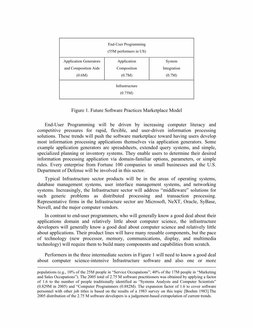
End-User Programming

(55M performers in US)

Application Generators Application System

and Composition Aids Composition Integration

(0.6M) (0.7M) (0.7M)

Infrastructure

(0.75M)

Figure 1. Future Software Practices Marketplace Model

End-User Programming will be driven by increasing computer literacy and competitive pressures for rapid, flexible, and user-driven information processing solutions. These trends will push the software marketplace toward having users develop most information processing applications themselves via application generators. Some example application generators are spreadsheets, extended query systems, and simple, specialized planning or inventory systems. They enable users to determine their desired information processing application via domain-familiar options, parameters, or simple rules. Every enterprise from Fortune 100 companies to small businesses and the U.S. Department of Defense will be involved in this sector.

Typical Infrastructure sector products will be in the areas of operating systems, database management systems, user interface management systems, and networking systems. Increasingly, the Infrastructure sector will address “middleware” solutions for such generic problems as distributed processing and transaction processing. Representative firms in the Infrastructure sector are Microsoft, NeXT, Oracle, SyBase, Novell, and the major computer vendors.

In contrast to end-user programmers, who will generally know a good deal about their applications domain and relatively little about computer science, the infrastructure developers will generally know a good deal about computer science and relatively little about applications. Their product lines will have many reusable components, but the pace of technology (new processor, memory, communications, display, and multimedia technology) will require them to build many components and capabilities from scratch.

Performers in the three intermediate sectors in Figure 1 will need to know a good deal about computer science-intensive Infrastructure software and also one or more populations (e.g., 10% of the 25M people in “Service Occupations”; 40% of the 17M people in “Marketing and Sales Occupations”). The 2005 total of 2.75 M software practitioners was obtained by applying a factor of 1.6 to the number of people traditionally identified as “Systems Analysts and Computer Scientists” (0.829M in 2005) and “Computer Programmers (0.882M). The expansion factor of 1.6 to cover software personnel with other job titles is based on the results of a 1983 survey on this topic [Boehm 1983].The 2005 distribution of the 2.75 M software developers is a judgement-based extrapolation of current trends.

applications domains. Creating this talent pool is a major national challenge.

The Application Generators sector will create largely prepackaged capabilities for user programming. Typical firms operating in this sector are Microsoft, Lotus, Novell, Borland, and vendors of computer-aided planning, engineering, manufacturing, and financial analysis systems. Their product lines will have many reusable components, but also will require a good deal of new-capability development from scratch. Application Composition Aids will be developed both by the firms above and by software product-line investments of firms in the Application Composition sector.

The Application Composition sector deals with applications which are too diversified to be handled by prepackaged solutions, but which are sufficiently simple to be rapidly composable from interoperable components. Typical components will be graphic user interface (GUI) builders, database or object managers, middleware for distributed processing or transaction processing, hypermedia handlers, smart data finders, and domain-specific components such as financial, medical, or industrial process control packages.

Most large firms will have groups to compose such applications, but a great many specialized software firms will provide composed applications on contract. These range from large, versatile firms such as Andersen Consulting and EDS, to small firms specializing in such specialty areas as decision support or transaction processing, or in such applications domains as finance or manufacturing.

The Systems Integration sector deals with large scale, highly embedded, or unprecedented systems. Portions of these systems can be developed with Application Composition capabilities, but their demands generally require a significant amount of up-front systems engineering and custom software development. Aerospace firms operate within this sector, as do major system integration firms such as EDS and Andersen Consulting, large firms developing software-intensive products and services (telecommunications, automotive, financial, and electronic products firms), and firms developing large-scale corporate information systems or manufacturing support systems.

3. COCOMO 2.0 STRATEGY AND RATIONALE The four main elements of the COCOMO 2.0 strategy are:

• Preserve the openness of the original COCOMO;

• Key the structure of COCOMO 2.0 to the future software marketplace sectors described above;

• Key the inputs and outputs of the COCOMO 2.0 submodels to the level of information available;

• Enable the COCOMO 2.0 submodels to be tailored to a project's particular process strategy.

COCOMO 2.0 follows the openness principles used in the original COCOMO. Thus, all of its relationships and algorithms will be publicly available. Also, all of its interfaces

are designed to be public, well-defined, and parametrized, so that complementary preprocessors (analogy, case-based, or other size estimation models), post-processors (project planning and control tools, project dynamics models, risk analyzers), and higher level packages (project management packages, product negotiation aids), can be combined straightforwardly with COCOMO 2.0.

To support the software marketplace sectors above, COCOMO 2.0 provides a family of increasingly detailed software cost estimation models, each tuned to the sectors' needs and type of information available to support software cost estimation.

3.1 COCOMO 2.0 Models for the Software Marketplace Sectors

The User Programming sector does not need a COCOMO 2.0 model. Its applications are typically developed in hours to days, so a simple activity-based estimate will generally be sufficient.

The COCOMO 2.0 model for the Application Composition sector is based on Object Points. Object Points are a count of the screens, reports and third-generation-language modules developed in the application, each weighted by a three-level (simple, medium, difficult) complexity factor [Banker et al. 1994, Kauffman and Kumar 1993]. This is commensurate with the level of information generally known about an Application Composition product during its planning stages, and the corresponding level of accuracy needed for its software cost estimates (such applications are generally developed by a small team in a few weeks to months).

The COCOMO 2.0 capability for estimation of Application Generator, System Integration, or Infrastructure developments is based on a tailorable mix of the Application Composition model (for early prototyping efforts) and two increasingly detailed estimation models for subsequent portions of the life cycle.

3.2 COCOMO 2.0 Model Rationale and Elaboration

The rationale for providing this tailorable mix of models rests on three primary premises.

First, unlike the initial COCOMO situation in the late 1970's, in which there was a single, preferred software life cycle model (the waterfall model), current and future software projects will be tailoring their processes to their particular process drivers. These process drivers include COTS or reusable software availability; degree of understanding of architectures and requirements; market window or other schedule constraints; size; and required reliability (see [Boehm 1989, pp. 436-37] for an example of such tailoring guidelines).

Second, the granularity of the software cost estimation model used needs to be consistent with the granularity of the information available to support software cost estimation. In the early stages of a software project, very little may be known about the size of the product to be developed, the nature of the target platform, the nature of the personnel to be involved in the project, or the detailed specifics of the process to be used.

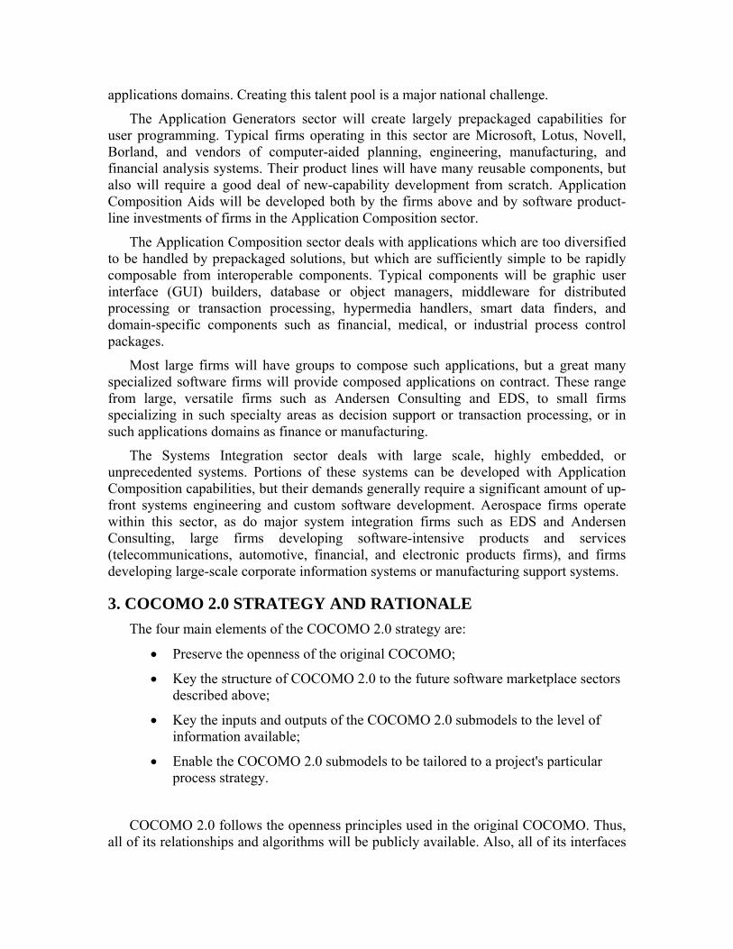
Figure 2, extended from [Boehm 1981, p. 311], indicates the effect of project uncertainties on the accuracy of software size and cost estimates. In the very early stages,

one may not know the specific nature of the product to be developed to better than a factor of 4. As the life cycle proceeds, and product decisions are made, the nature of the products and its consequent size are better known, and the nature of the process and its consequent cost drivers are better known. The earlier “completed programs” size and effort data points in Figure 2 are the actual sizes and efforts of seven software products built to an imprecisely-defined specification [Boehm et al. 1984]‡. The later “USAF/ESD proposals” data points are from five proposals submitted to the U.S. Air Force Electronic Systems Division in response to a fairly thorough specification [Devenny 1976].

Figure 2. Software Costing and Sizing Accuracy vs. Phase

Third, given the situation in premises 1 and 2, COCOMO 2.0 enables projects to furnish coarse grained cost driver information in the early project stages, and increasingly fine-grained information in later stages. Consequently, COCOMO 2.0 does not produce point estimates of software cost and effort, but rather range estimates tied to the degree of definition of the estimation inputs. The uncertainty ranges in Figure 2 are used as starting points for these estimation ranges.

With respect to process strategy, Application Generator, System Integration, and Infrastructure software projects will involve a mix of three major process models. The appropriate sequencing of these models will depend on the project’s marketplace drivers ‡ These seven projects implemented the same algorithmic version of the Intermediate COCOMO cost model, but with the use of different interpretations of the other product specifications: produce a “friendly user inter-face” with a “single-user file system.”

and degree of product understanding.

The Application Composition model involves prototyping efforts to resolve potential high-risk issues such as user interfaces, software/system interaction, performance, or technology maturity. The costs of this type of effort are best estimated by the Applications Composition model.

The Early Design model involves exploration of alternative software/system architectures and concepts of operation. At this stage, not enough is generally known to support fine-grain cost estimation. The corresponding COCOMO 2.0 capability involves the use of function points and a small number of additional cost drivers.

The Post-Architecture model involves the actual development and maintenance of a software product. This model proceeds most cost-effectively if a software life-cycle architecture has been developed; validated with respect to the system's mission, concept of operation, and risk; and established as the framework for the product. The corresponding COCOMO 2.0 model has about the same granularity as the previous COCOMO and Ada COCOMO models. It uses source instructions and / or function points for sizing, with modifiers for reuse and software breakage; a set of 17 multiplicative cost drivers; and a set of 5 factors determining the project's scaling exponent. These factors replace the development modes (Organic, Semidetached, or Embedded) in the original COCOMO model, and refine the four exponent-scaling factors in Ada COCOMO.

To summarize, COCOMO 2.0 provides the following three-model series for estimation of Application Generator, System Integration, and Infrastructure software projects:

1. The earliest phases or spiral cycles will generally involve prototyping, using Application Composition capabilities. The COCOMO 2.0 Application Composition model supports these phases, and any other prototyping activities occurring later in the life cycle.

2. The next phases or spiral cycles will generally involve exploration of architectural alternatives or incremental development strategies. To support these activities, COCOMO 2.0 provides an early estimation model. This uses function points for sizing, and a coarse-grained set of 5 cost drivers (e.g., two cost drivers for Personnel Capability and Personnel Experience in place of the 6 current Post-Architecture model cost drivers covering various aspects of personnel capability, continuity and experience). Again, this level of detail is consistent with the general level of information available and the general level of estimation accuracy needed at this stage.

3. Once the project is ready to develop and sustain a fielded system, it should have a life-cycle architecture, which provides more accurate information on cost driver inputs, and enables more accurate cost estimates. To support this stage of development, COCOMO 2.0 provides a model whose granularity is roughly equivalent to the current COCOMO and Ada COCOMO models. It can use either source lines of code or function points for a sizing parameter, a refinement of the COCOMO development modes as a scaling factor, and 17

multiplicative cost drivers.

The above should be considered as current working hypotheses about the most effective forms for COCOMO 2.0. They will be subject to revision based on subsequent data analysis. Data analysis should also enable the further calibration of the relationships between object points, function points, and source lines of code for various languages and composition systems, enabling flexibility in the choice of sizing parameters.

3.3 Other Major Differences Between COCOMO and COCOMO 2.0

The tailorable mix of models and variable-granularity cost model inputs and outputs are not the only differences between the original COCOMO and COCOMO 2.0. The other major differences involve size-related effects involving reuse and re-engineering, changes in scaling effects, and changes in cost drivers. These are summarized in Table 1, and elaborated in Sections 4, 5, and 6 below. Explanations of the acronyms and abbreviations in Table 1 are provided in Section 9.

4. Cost Factors: Sizing This Section provides the definitions and rationale for the three sizing quantities used

in COCOMO 2.0: Object Points, Unadjusted Function Points, and Source Lines of Code. It then discusses the COCOMO 2.0 size-related parameters used in dealing with software reuse, re-engineering, conversion, and maintenance.

4.1 Applications Composition: Object Points

Object Point estimation is a relatively new software sizing approach, but it is well-matched to the practices in the Applications Composition sector. It is also a good match to associated prototyping efforts, based on the use of a rapid-composition Integrated Computer Aided Software Environment (ICASE) providing graphic user interface builders, software development tools, and large, composable infrastructure and applications components. In these areas, it has compared well to Function Point estimation on a nontrivial (but still limited) set of applications.

The [Banker et al. 1994] comparative study of Object Point vs. Function Point estimation analyzed a sample of 19 investment banking software projects from a single organization, developed using ICASE applications composition capabilities, and ranging from 4.7 to 71.9 person-months of effort. The study found that the Object Points approach explained 73% of the variance (R

2) in person-months adjusted for reuse, as

compared to 76% for Function Points.

A subsequent statistically-designed experiment [Kaufman and Kumar 1993] involved four experienced project managers using Object Points and Function Points to estimate the effort required on two completed projects (3.5 and 6 actual person-months), based on project descriptions of the type available at the beginning of such projects. The experiment found that Object Points and Function Points produced comparably accurate results (slightly more accurate with Object Points, but not statistically significant). From a usage standpoint, the average time to produce an Object Point estimate was about 47% of the corresponding average time for Function Point estimates. Also, the managers considered the Object Point method easier to use (both of these results were statistically

significant).

Thus, although these results are not yet broadly-based, their match to Applications Composition software development appears promising enough to justify selecting Object Points as the starting point for the COCOMO 2.0 Applications Composition estimation model.

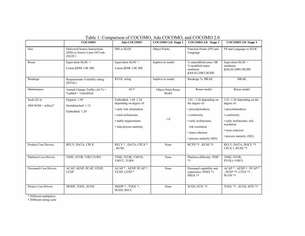
Table 1: Comparison of COCOMO, Ada COCOMO, and COCOMO 2.0 COCOMO Ada COCOMO COCOMO 2.0: Stage 1 COCOMO 2.0: Stage 2 COCOMO 2.0: Stage 3

Size Delivered Source Instructions (DSI) or Source Lines Of Code (SLOC)

DSI or SLOC Object Points Function Points (FP) and Language

FP and Language or SLOC

Reuse Equivalent SLOC =

Linear f(DM, CM, IM)

Equivalent SLOC =

Linear f(DM, CM, IM)

Implicit in model % unmodified reuse: SR % modified reuse: nonlinear f(AA,SU,DM,CM,IM)

Equivalent SLOC = nonlinear f(AA,SU,DM,CM,IM)

Breakage Requirements Volatility rating: (RVOL)

RVOL rating Implicit in model Breakage %: BRAK BRAK

Maintenance Annual Change Traffic (ACT) = %added + %modified

ACT Object Point Reuse Model

Reuse model Reuse model

Scale (b) in

MM NOM = a(Size)b

Organic: 1.05

Semidetached: 1.12

Embedded: 1.20

Embedded: 1.04 -1.24 depending on degree of:

• early risk elimination

• solid architecture

• stable requirements

• Ada process maturity

1.0

1.01 - 1.26 depending on the degree of:

• precedentedness

• conformity

• early architecture,

risk resolution

• team cohesion

• process maturity (SEI)

1.01 -1.26 depending on the degree of:

• precedentedness

• conformity

• early architecture, risk resolution

• team cohesion

• process maturity (SEI)

Product Cost Drivers RELY, DATA, CPLX RELY * , DATA, CPLX * , RUSE

None RCPX *† , RUSE *† RELY, DATA, DOCU *† CPLX †, RUSE *†

Platform Cost Drivers TIME, STOR, VIRT,TURN TIME, STOR, VMVH, VMVT, TURN

None Platform difficulty: PDIF *†

TIME, STOR, PVOL(=VIRT)

Personnel Cost Drivers ACAP, AEXP, PCAP, VEXP, LEXP

ACAP * , AEXP, PCAP *, VEXP, LEXP *

None Personnel capability and experience: PERS *†, PREX *†

ACAP * , AEXP † , PCAP * , PEXP *†, LTEX *† , PCON *†

Project Cost Drivers MODP, TOOL, SCED MODP * , TOOL * , SCED, SECU

None SCED, FCIL *† TOOL *† , SCED, SITE *†

* Different multipliers. † Different rating scale

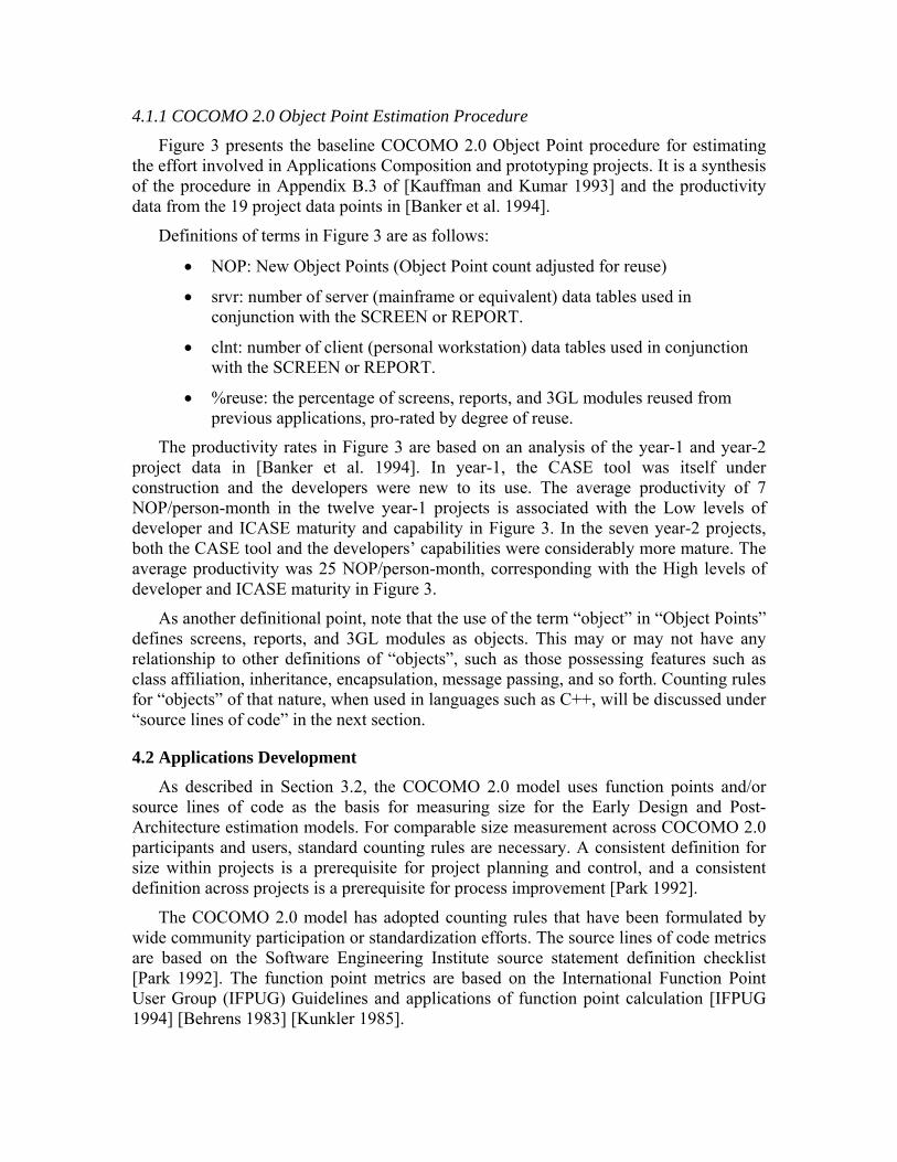
4.1.1 COCOMO 2.0 Object Point Estimation Procedure

Figure 3 presents the baseline COCOMO 2.0 Object Point procedure for estimating the effort involved in Applications Composition and prototyping projects. It is a synthesis of the procedure in Appendix B.3 of [Kauffman and Kumar 1993] and the productivity data from the 19 project data points in [Banker et al. 1994].

Definitions of terms in Figure 3 are as follows:

• NOP: New Object Points (Object Point count adjusted for reuse)

• srvr: number of server (mainframe or equivalent) data tables used in conjunction with the SCREEN or REPORT.

• clnt: number of client (personal workstation) data tables used in conjunction with the SCREEN or REPORT.

• %reuse: the percentage of screens, reports, and 3GL modules reused from previous applications, pro-rated by degree of reuse.

The productivity rates in Figure 3 are based on an analysis of the year-1 and year-2 project data in [Banker et al. 1994]. In year-1, the CASE tool was itself under construction and the developers were new to its use. The average productivity of 7 NOP/person-month in the twelve year-1 projects is associated with the Low levels of developer and ICASE maturity and capability in Figure 3. In the seven year-2 projects, both the CASE tool and the developers’ capabilities were considerably more mature. The average productivity was 25 NOP/person-month, corresponding with the High levels of developer and ICASE maturity in Figure 3.

As another definitional point, note that the use of the term “object” in “Object Points” defines screens, reports, and 3GL modules as objects. This may or may not have any relationship to other definitions of “objects”, such as those possessing features such as class affiliation, inheritance, encapsulation, message passing, and so forth. Counting rules for “objects” of that nature, when used in languages such as C++, will be discussed under “source lines of code” in the next section.

4.2 Applications Development

As described in Section 3.2, the COCOMO 2.0 model uses function points and/or source lines of code as the basis for measuring size for the Early Design and Post-Architecture estimation models. For comparable size measurement across COCOMO 2.0 participants and users, standard counting rules are necessary. A consistent definition for size within projects is a prerequisite for project planning and control, and a consistent definition across projects is a prerequisite for process improvement [Park 1992].

The COCOMO 2.0 model has adopted counting rules that have been formulated by wide community participation or standardization efforts. The source lines of code metrics are based on the Software Engineering Institute source statement definition checklist [Park 1992]. The function point metrics are based on the International Function Point User Group (IFPUG) Guidelines and applications of function point calculation [IFPUG 1994] [Behrens 1983] [Kunkler 1985].

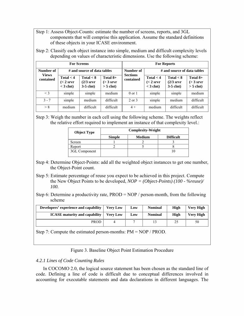
Step 1: Assess Object-Counts: estimate the number of screens, reports, and 3GL components that will comprise this application. Assume the standard definitions of these objects in your ICASE environment.

Step 2: Classify each object instance into simple, medium and difficult complexity levels depending on values of characteristic dimensions. Use the following scheme:

For Screens For Reports

# and source of data tables # and source of data tables Number of Views

contained Total < 4 (< 2 srvr < 3 clnt)

Total < 8 (2/3 srvr 3-5 clnt)

Total 8+ (> 3 srvr > 5 clnt)

Number of Sections contained Total < 4

(< 2 srvr < 3 clnt)

Total < 8 (2/3 srvr 3-5 clnt)

Total 8+ (> 3 srvr > 5 clnt)

< 3 simple simple medium 0 or 1 simple simple medium

3 - 7 simple medium difficult 2 or 3 simple medium difficult

> 8 medium difficult difficult 4 + medium difficult difficult

Step 3: Weigh the number in each cell using the following scheme. The weights reflect the relative effort required to implement an instance of that complexity level.:

Complexity-Weight Object Type Simple Medium Difficult

Screen 1 2 3 Report 2 5 8 3GL Component 10

Step 4: Determine Object-Points: add all the weighted object instances to get one number, the Object-Point count.

Step 5: Estimate percentage of reuse you expect to be achieved in this project. Compute the New Object Points to be developed, NOP = (Object-Points) (100 - %reuse)/ 100.

Step 6: Determine a productivity rate, PROD = NOP / person-month, from the following scheme

Developers’ experience and capability Very Low Low Nominal High Very High

ICASE maturity and capability Very Low Low Nominal High Very High

PROD 4 7 13 25 50

Step 7: Compute the estimated person-months: PM = NOP / PROD.

Figure 3. Baseline Object Point Estimation Procedure

4.2.1 Lines of Code Counting Rules

In COCOMO 2.0, the logical source statement has been chosen as the standard line of code. Defining a line of code is difficult due to conceptual differences involved in accounting for executable statements and data declarations in different languages. The

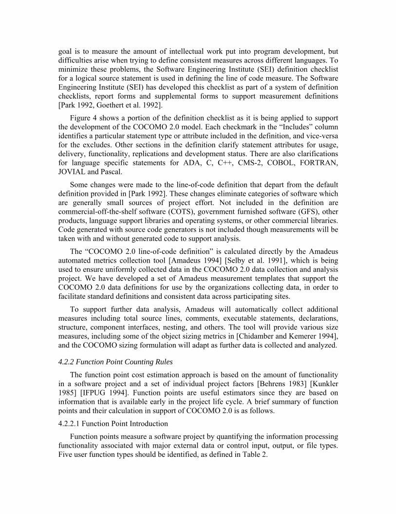
goal is to measure the amount of intellectual work put into program development, but difficulties arise when trying to define consistent measures across different languages. To minimize these problems, the Software Engineering Institute (SEI) definition checklist for a logical source statement is used in defining the line of code measure. The Software Engineering Institute (SEI) has developed this checklist as part of a system of definition checklists, report forms and supplemental forms to support measurement definitions [Park 1992, Goethert et al. 1992].

Figure 4 shows a portion of the definition checklist as it is being applied to support the development of the COCOMO 2.0 model. Each checkmark in the “Includes” column identifies a particular statement type or attribute included in the definition, and vice-versa for the excludes. Other sections in the definition clarify statement attributes for usage, delivery, functionality, replications and development status. There are also clarifications for language specific statements for ADA, C, C++, CMS-2, COBOL, FORTRAN, JOVIAL and Pascal.

Some changes were made to the line-of-code definition that depart from the default definition provided in [Park 1992]. These changes eliminate categories of software which are generally small sources of project effort. Not included in the definition are commercial-off-the-shelf software (COTS), government furnished software (GFS), other products, language support libraries and operating systems, or other commercial libraries. Code generated with source code generators is not included though measurements will be taken with and without generated code to support analysis.

The “COCOMO 2.0 line-of-code definition” is calculated directly by the Amadeus automated metrics collection tool [Amadeus 1994] [Selby et al. 1991], which is being used to ensure uniformly collected data in the COCOMO 2.0 data collection and analysis project. We have developed a set of Amadeus measurement templates that support the COCOMO 2.0 data definitions for use by the organizations collecting data, in order to facilitate standard definitions and consistent data across participating sites.

To support further data analysis, Amadeus will automatically collect additional measures including total source lines, comments, executable statements, declarations, structure, component interfaces, nesting, and others. The tool will provide various size measures, including some of the object sizing metrics in [Chidamber and Kemerer 1994], and the COCOMO sizing formulation will adapt as further data is collected and analyzed.

4.2.2 Function Point Counting Rules

The function point cost estimation approach is based on the amount of functionality in a software project and a set of individual project factors [Behrens 1983] [Kunkler 1985] [IFPUG 1994]. Function points are useful estimators since they are based on information that is available early in the project life cycle. A brief summary of function points and their calculation in support of COCOMO 2.0 is as follows.

4.2.2.1 Function Point Introduction

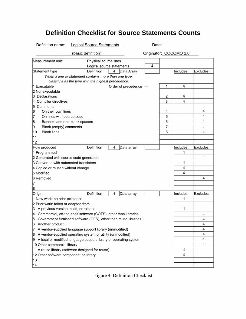
Function points measure a software project by quantifying the information processing functionality associated with major external data or control input, output, or file types. Five user function types should be identified, as defined in Table 2.

Definition Checklist for Source Statements Counts

Definition name: __Logical Source Statements__ Date:________________

________________(basic definition)__________ Originator:_COCOMO 2.0____

Measurement unit: Physical source lines Logical source statements 4 Statement type Definition 4 Data Array Includes Excludes

When a line or statement contains more than one type, classify it as the type with the highest precedence.

1 Executable Order of precedence → 1 4 2 Nonexecutable 3 Declarations 2 4 4 Compiler directives 3 4 5 Comments 6 On their own lines 4 4 7 On lines with source code 5 4 8 Banners and non-blank spacers 6 4 9 Blank (empty) comments 7 4 10 Blank lines 8 4 11 12 How produced Definition 4 Data array Includes Excludes 1 Programmed 4 2 Generated with source code generators 4 3 Converted with automated translators 4 4 Copied or reused without change 4 5 Modified 4 6 Removed 4 7 8 Origin Definition 4 Data array Includes Excludes 1 New work: no prior existence 4 2 Prior work: taken or adapted from 3 A previous version, build, or release 4 4 Commercial, off-the-shelf software (COTS), other than libraries 4 5 Government furnished software (GFS), other than reuse libraries 4 6 Another product 4 7 A vendor-supplied language support library (unmodified) 4 8 A vendor-supplied operating system or utility (unmodified) 4 9 A local or modified language support library or operating system 4 10 Other commercial library 4 11 A reuse library (software designed for reuse) 4 12 Other software component or library 4 13 14

Figure 4. Definition Checklist

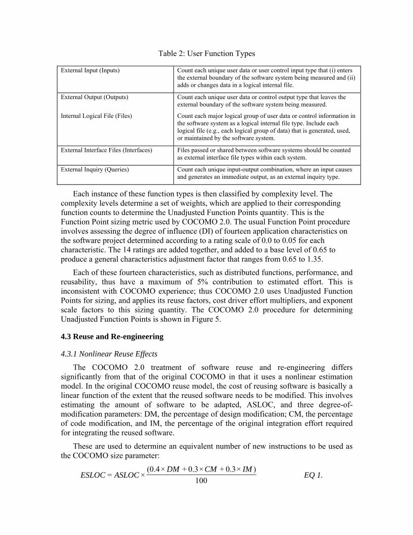
Table 2: User Function Types

External Input (Inputs) Count each unique user data or user control input type that (i) enters the external boundary of the software system being measured and (ii) adds or changes data in a logical internal file.

External Output (Outputs) Count each unique user data or control output type that leaves the external boundary of the software system being measured.

Internal Logical File (Files) Count each major logical group of user data or control information in the software system as a logical internal file type. Include each logical file (e.g., each logical group of data) that is generated, used, or maintained by the software system.

External Interface Files (Interfaces) Files passed or shared between software systems should be counted as external interface file types within each system.

External Inquiry (Queries) Count each unique input-output combination, where an input causes and generates an immediate output, as an external inquiry type.

Each instance of these function types is then classified by complexity level. The complexity levels determine a set of weights, which are applied to their corresponding function counts to determine the Unadjusted Function Points quantity. This is the Function Point sizing metric used by COCOMO 2.0. The usual Function Point procedure involves assessing the degree of influence (DI) of fourteen application characteristics on the software project determined according to a rating scale of 0.0 to 0.05 for each characteristic. The 14 ratings are added together, and added to a base level of 0.65 to produce a general characteristics adjustment factor that ranges from 0.65 to 1.35.

Each of these fourteen characteristics, such as distributed functions, performance, and reusability, thus have a maximum of 5% contribution to estimated effort. This is inconsistent with COCOMO experience; thus COCOMO 2.0 uses Unadjusted Function Points for sizing, and applies its reuse factors, cost driver effort multipliers, and exponent scale factors to this sizing quantity. The COCOMO 2.0 procedure for determining Unadjusted Function Points is shown in Figure 5.

4.3 Reuse and Re-engineering

4.3.1 Nonlinear Reuse Effects

The COCOMO 2.0 treatment of software reuse and re-engineering differs significantly from that of the original COCOMO in that it uses a nonlinear estimation model. In the original COCOMO reuse model, the cost of reusing software is basically a linear function of the extent that the reused software needs to be modified. This involves estimating the amount of software to be adapted, ASLOC, and three degree-of-modification parameters: DM, the percentage of design modification; CM, the percentage of code modification, and IM, the percentage of the original integration effort required for integrating the reused software.

These are used to determine an equivalent number of new instructions to be used as the COCOMO size parameter:

100)× 0.3+×0.3+×(0.4

× = IMCMDM

ASLOCESLOC EQ 1.

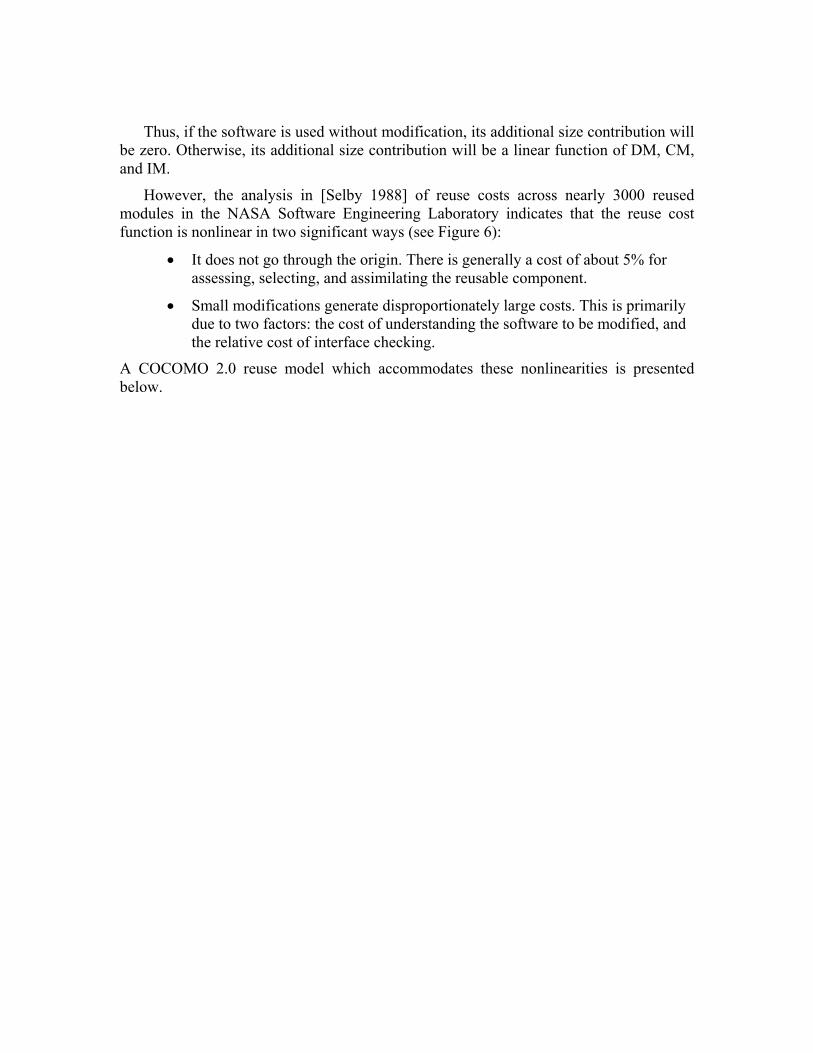
Thus, if the software is used without modification, its additional size contribution will be zero. Otherwise, its additional size contribution will be a linear function of DM, CM, and IM.

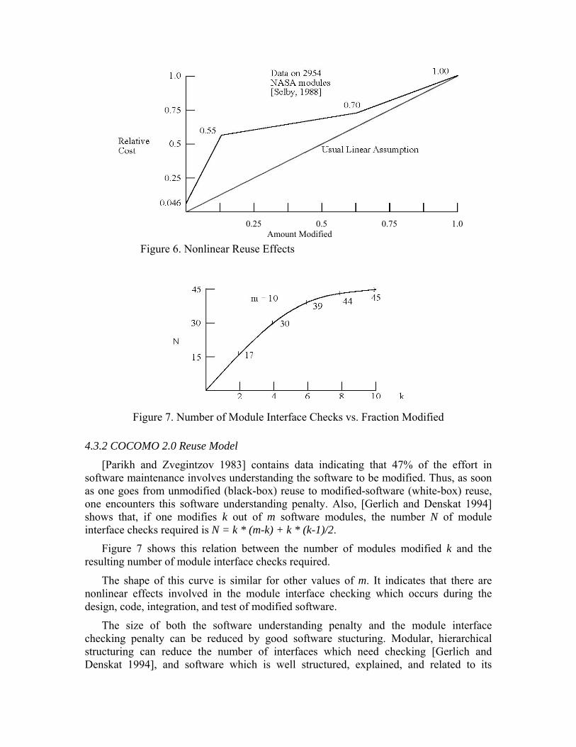
However, the analysis in [Selby 1988] of reuse costs across nearly 3000 reused modules in the NASA Software Engineering Laboratory indicates that the reuse cost function is nonlinear in two significant ways (see Figure 6):

• It does not go through the origin. There is generally a cost of about 5% for assessing, selecting, and assimilating the reusable component.

• Small modifications generate disproportionately large costs. This is primarily due to two factors: the cost of understanding the software to be modified, and the relative cost of interface checking.

A COCOMO 2.0 reuse model which accommodates these nonlinearities is presented below.

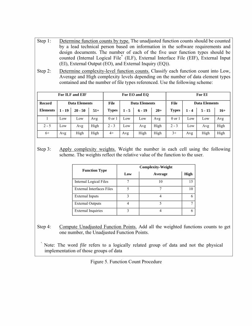
Step 1: Determine function counts by type. The unadjusted function counts should be counted by a lead technical person based on information in the software requirements and design documents. The number of each of the five user function types should be counted (Internal Logical File* (ILF), External Interface File (EIF), External Input (EI), External Output (EO), and External Inquiry (EQ)).

Step 2: Determine complexity-level function counts. Classify each function count into Low, Average and High complexity levels depending on the number of data element types contained and the number of file types referenced. Use the following scheme:

For ILF and EIF For EO and EQ For EI

Record Data Elements File Data Elements File Data Elements

Elements 1 - 19 20 - 50 51+ Types 1 - 5 6 - 19 20+ Types 1 - 4 5 - 15 16+

1 Low Low Avg 0 or 1 Low Low Avg 0 or 1 Low Low Avg

2 - 5 Low Avg High 2 - 3 Low Avg High 2 - 3 Low Avg High

6+ Avg High High 4+ Avg High High 3+ Avg High High

Step 3: Apply complexity weights. Weight the number in each cell using the following scheme. The weights reflect the relative value of the function to the user.

Complexity-Weight Function Type

Low Average High

Internal Logical Files 7 10 15

External Interfaces Files 5 7 10

External Inputs 3 4 6

External Outputs 4 5 7

External Inquiries 3 4 6

Step 4: Compute Unadjusted Function Points. Add all the weighted functions counts to get one number, the Unadjusted Function Points.

*. Note: The word file refers to a logically related group of data and not the physical implementation of those groups of data

Figure 5. Function Count Procedure

0.25 0.5 0.75 1.0

Amount Modified

Figure 6. Nonlinear Reuse Effects

Figure 7. Number of Module Interface Checks vs. Fraction Modified

4.3.2 COCOMO 2.0 Reuse Model

[Parikh and Zvegintzov 1983] contains data indicating that 47% of the effort in software maintenance involves understanding the software to be modified. Thus, as soon as one goes from unmodified (black-box) reuse to modified-software (white-box) reuse, one encounters this software understanding penalty. Also, [Gerlich and Denskat 1994] shows that, if one modifies k out of m software modules, the number N of module interface checks required is N = k * (m-k) + k * (k-1)/2.

Figure 7 shows this relation between the number of modules modified k and the resulting number of module interface checks required.

The shape of this curve is similar for other values of m. It indicates that there are nonlinear effects involved in the module interface checking which occurs during the design, code, integration, and test of modified software.

The size of both the software understanding penalty and the module interface checking penalty can be reduced by good software stucturing. Modular, hierarchical structuring can reduce the number of interfaces which need checking [Gerlich and Denskat 1994], and software which is well structured, explained, and related to its

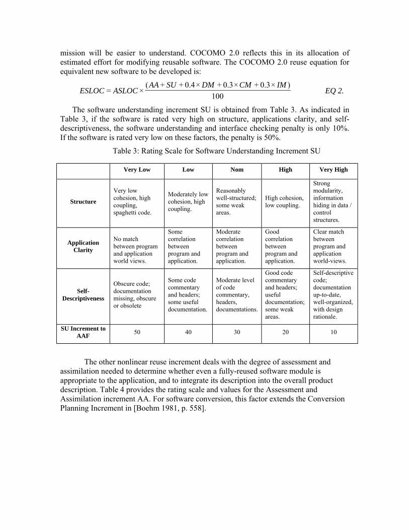
mission will be easier to understand. COCOMO 2.0 reflects this in its allocation of estimated effort for modifying reusable software. The COCOMO 2.0 reuse equation for equivalent new software to be developed is:

100)×3.0+× 0.3+×0.4++(

× = IMCMDMSUAA

ASLOCESLOC EQ 2.

The software understanding increment SU is obtained from Table 3. As indicated in Table 3, if the software is rated very high on structure, applications clarity, and self-descriptiveness, the software understanding and interface checking penalty is only 10%. If the software is rated very low on these factors, the penalty is 50%.

Table 3: Rating Scale for Software Understanding Increment SU

Very Low Low Nom High Very High

Structure Very low cohesion, high coupling, spaghetti code.

Moderately low cohesion, high coupling.

Reasonably well-structured; some weak areas.

High cohesion, low coupling.

Strong modularity, information hiding in data / control structures.

Application Clarity

No match between program and application world views.

Some correlation between program and application.

Moderate correlation between program and application.

Good correlation between program and application.

Clear match between program and application world-views.

Self-Descriptiveness

Obscure code; documentation missing, obscure or obsolete

Some code commentary and headers; some useful documentation.

Moderate level of code commentary, headers, documentations.

Good code commentary and headers; useful documentation; some weak areas.

Self-descriptive code; documentation up-to-date, well-organized, with design rationale.

SU Increment to AAF 50 40 30 20 10

The other nonlinear reuse increment deals with the degree of assessment and assimilation needed to determine whether even a fully-reused software module is appropriate to the application, and to integrate its description into the overall product description. Table 4 provides the rating scale and values for the Assessment and Assimilation increment AA. For software conversion, this factor extends the Conversion Planning Increment in [Boehm 1981, p. 558].

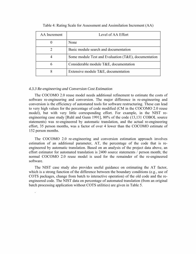
Table 4: Rating Scale for Assessment and Assimilation Increment (AA)

AA Increment Level of AA Effort

0 None

2 Basic module search and documentation

4 Some module Test and Evaluation (T&E), documentation

6 Considerable module T&E, documentation

8 Extensive module T&E, documentation

4.3.3 Re-engineering and Conversion Cost Estimation

The COCOMO 2.0 reuse model needs additional refinement to estimate the costs of software re-engineering and conversion. The major difference in re-engineering and conversion is the efficiency of automated tools for software restructuring. These can lead to very high values for the percentage of code modified (CM in the COCOMO 2.0 reuse model), but with very little corresponding effort. For example, in the NIST re-engineering case study [Ruhl and Gunn 1991], 80% of the code (13,131 COBOL source statements) was re-engineered by automatic translation, and the actual re-engineering effort, 35 person months, was a factor of over 4 lower than the COCOMO estimate of 152 person months.

The COCOMO 2.0 re-engineering and conversion estimation approach involves estimation of an additional parameter, AT, the percentage of the code that is re-engineered by automatic translation. Based on an analysis of the project data above, an effort estimator for automated translation is 2400 source statements / person month; the normal COCOMO 2.0 reuse model is used for the remainder of the re-engineered software.

The NIST case study also provides useful guidance on estimating the AT factor, which is a strong function of the difference between the boundary conditions (e.g., use of COTS packages, change from batch to interactive operation) of the old code and the re-engineered code. The NIST data on percentage of automated translation (from an original batch processing application without COTS utilities) are given in Table 5.

.

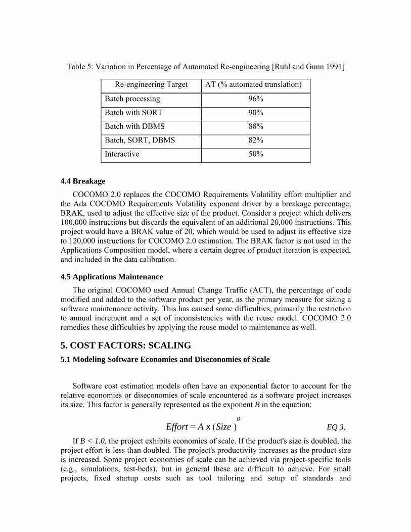
Table 5: Variation in Percentage of Automated Re-engineering [Ruhl and Gunn 1991]

Re-engineering Target AT (% automated translation)

Batch processing 96%

Batch with SORT 90%

Batch with DBMS 88%

Batch, SORT, DBMS 82%

Interactive 50%

4.4 Breakage

COCOMO 2.0 replaces the COCOMO Requirements Volatility effort multiplier and the Ada COCOMO Requirements Volatility exponent driver by a breakage percentage, BRAK, used to adjust the effective size of the product. Consider a project which delivers 100,000 instructions but discards the equivalent of an additional 20,000 instructions. This project would have a BRAK value of 20, which would be used to adjust its effective size to 120,000 instructions for COCOMO 2.0 estimation. The BRAK factor is not used in the Applications Composition model, where a certain degree of product iteration is expected, and included in the data calibration.

4.5 Applications Maintenance

The original COCOMO used Annual Change Traffic (ACT), the percentage of code modified and added to the software product per year, as the primary measure for sizing a software maintenance activity. This has caused some difficulties, primarily the restriction to annual increment and a set of inconsistencies with the reuse model. COCOMO 2.0 remedies these difficulties by applying the reuse model to maintenance as well.

5. COST FACTORS: SCALING 5.1 Modeling Software Economies and Diseconomies of Scale

Software cost estimation models often have an exponential factor to account for the relative economies or diseconomies of scale encountered as a software project increases its size. This factor is generally represented as the exponent B in the equation:

Effort = A X (Size )B

EQ 3.

If B < 1.0, the project exhibits economies of scale. If the product's size is doubled, the project effort is less than doubled. The project's productivity increases as the product size is increased. Some project economies of scale can be achieved via project-specific tools (e.g., simulations, test-beds), but in general these are difficult to achieve. For small projects, fixed startup costs such as tool tailoring and setup of standards and

administrative reports are often a source of economies of scale.

If B = 1.0, the economies and diseconomies of scale are in balance. This linear model is often used for cost estimation of small projects. It is used for the COCOMO 2.0 Applications Composition model.

If B > 1.0, the project exhibits diseconomies of scale. This is generally due to two main factors: growth of interpersonal communications overhead and growth of large-system integration overhead. Larger projects will have more personnel, and thus more interpersonal communications paths consuming overhead. Integrating a small product as part of a larger product requires not only the effort to develop the small product, but also the additional overhead effort to design, maintain, integrate, and test its interfaces with the remainder of the product.

See [Banker et al 1994a] for a further discussion of software economies and diseconomies of scale.

The COCOMO 2.0 value for the coefficient A in EQ 3 is provisionally set at 3.0 Initial calibration of COCOMO 2.0 to the original COCOMO project database [Boehm 1981, pp. 496-97] indicates that this is a reasonable starting point.

5.2 COCOMO and Ada COCOMO Scaling Approaches

The data analysis on the original COCOMO indicated that its projects exhibited net diseconomies of scale. The projects factored into three classes or modes of software development (Organic, Semidetached, and Embedded), whose exponents B were 1.05, 1.12, and 1.20, respectively. The distinguishing factors of these modes were basically environmental: Embedded-mode projects were more unprecedented, requiring more communication overhead and complex integration; and less flexible, requiring more communications overhead and extra effort to resolve issues within tight schedule, budget, interface, and performance constraints.

The scaling model in Ada COCOMO continued to exhibit diseconomies of scale, but recognized that a good deal of the diseconomy could be reduced via management controllables. Communications overhead and integration overhead could be reduced significantly by early risk and error elimination; by using thorough, validated architectural specifications; and by stabilizing requirements. These practices were combined into an Ada process model [Boehm and Royce 1989, Royce 1990]. The project's use of these practices, and an Ada process model experience or maturity factor, were used in Ada COCOMO to determine the scale factor B.

Ada COCOMO applied this approach to only one of the COCOMO development modes, the Embedded mode. Rather than a single exponent B = 1.20 for this mode, Ada COCOMO enabled B to vary from 1.04 to 1.24, depending on the project's progress in reducing diseconomies of scale via early risk elimination, solid architecture, stable requirements, and Ada process maturity.

5.3 COCOMO 2.0 Scaling Approach

COCOMO 2.0 combines the COCOMO and Ada COCOMO scaling approaches into a single rating-driven model. It is similar to that of Ada COCOMO in having additive

factors applied to a base exponent B. It includes the Ada COCOMO factors, but combines the architecture and risk factors into a single factor, and replaces the Ada process maturity factor with a Software Engineering Institute (SEI) process maturity factor (The exact form of this factor is still being worked out with the SEI). The scaling model also adds two factors, precedentedness and flexibility, to account for the mode effects in original COCOMO, and adds a Team Cohesiveness factor to account for the diseconomy-of-scale effects on software projects whose developers, customers, and users have difficulty in synchronizing their efforts. It does not include the Ada COCOMO Requirements Volatility factor, which is now covered by increasing the effective product size via the Breakage factor.

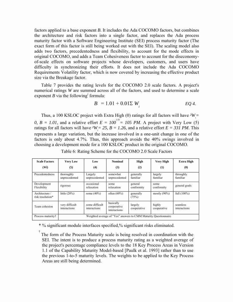
Table 7 provides the rating levels for the COCOMO 2.0 scale factors. A project's numerical ratings W are summed across all of the factors, and used to determine a scale exponent B via the followingi formula:

B = 1.01 + 0.01Σ Wi

EQ 4.

Thus, a 100 KSLOC project with Extra High (0) ratings for all factors will have ²Wi=

0, B = 1.01, and a relative effort E = 1001.01

= 105 PM. A project with Very Low (5) ratings for all factors will have ²W

i= 25, B = 1.26, and a relative effort E = 331 PM. This

represents a large variation, but the increase involved in a one-unit change in one of the factors is only about 4.7%. Thus, this approach avoids the 40% swings involved in choosing a development mode for a 100 KSLOC product in the original COCOMO.

Table 6: Rating Scheme for the COCOMO 2.0 Scale Factors

Scale Factors

(Wi)

Very Low

(5)

Low

(4)

Nominal

(3)

High

(2)

Very High

(1)

Extra High

(0)

Precedentedness thoroughly unprecedented

Largely unprecedented

somewhat unprecedented

generally familiar

largely familiar

throughly familiar

Development Flexibility rigorous occasional

relaxation some relaxation

general conformity

some conformity general goals

Architecture / risk resolution*

little (20%) some (40%) often (60%) generally (75%)

mostly (90%) full (100%)

Team cohesion very difficult interactions

some difficult interactions

basically cooperative interactions

largely cooperative

highly cooperative

seamless interactions

Process maturity† Weighted average of “Yes” answers to CMM Maturity Questionnaire

* % significant module interfaces specified,% significant risks eliminated. †

The form of the Process Maturity scale is being resolved in coordination with the SEI. The intent is to produce a process maturity rating as a weighted average of the project's percentage compliance levels to the 18 Key Process Areas in Version 1.1 of the Capability Maturity Model-based [Paulk et al. 1993] rather than to use the previous 1-to-5 maturity levels. The weights to be applied to the Key Process Areas are still being determined.

6. Cost Factors: Effort-Multiplier Cost Drivers COCOMO 2.0 continues the COCOMO and Ada COCOMO practice of using a set of

effort multipliers to adjust the nominal person-month estimate obtained from the project’s size and exponent drivers:

( ∏×=i

inominaladjusted EMPMPM ) EQ 5.

The primary selection and definition criteria for COCOMO 2.0 effort-multiplier cost drivers were:

• Continuity. Unless there has been a strong rationale otherwise, the COCOMO 2.0 baseline rating scales and effort multipliers are consistent with those in COCOMO and Ada COCOMO.

• Parsimony. Effort-multiplier cost drivers are included in the COCOMO 2.0 baseline model only if there has been a strong rationale that they would independently explain a significant source of project effort or productivity variation.

Table 7 summarizes the COCOMO 2.0 effort-multiplier cost drivers by the four categories of Product, Platform, Personnel, and Project Factors. The superscripts following the cost driver names indicated the differences between the COCOMO 2.0 cost drivers and their counterparts in COCOMO and Ada COCOMO:

blank - No difference in rating scales or effort multipliers

* - Same rating scales, different effort multipliers

† - Different rating scales, different effort multipliers

Table 7 provides the COCOMO 2.0 effort multiplier rating scales. The following subsections elaborate on the treatment of these effort-multiplier cost drivers, and discuss those which have been dropped in COCOMO 2.0.

6.1 Product Factors

6.1.1 RELY- Required Software Reliability

COCOMO 2.0 retains the original COCOMO RELY rating scales and effort multipliers. Ada COCOMO contained a lower set of effort multiplier values for the higher RELY levels, based on a rationale that Ada’s strong typing, tasking, exceptions, and other features eliminated significant classes of potential defects. Given the absence of strong evidence of a general effort-multiplier trend in this direction, the COCOMO 2.0 baseline RELY multipliers have not been changed from the original COCOMO, in consonance with the continuity criterion above.

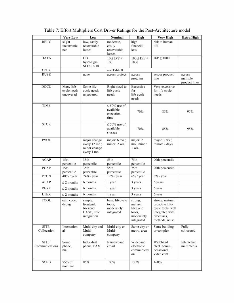
Table 7: Effort Multipliers Cost Driver Ratings for the Post-Architecture model Very Low Low Nominal High Very High Extra High

RELY slight inconvenience

low, easily recoverable losses

moderate, easily recoverable losses

high financial loss

risk to human life

DATA DB bytes/Pgm SLOC < 10

10 ≤ D/P < 100

100 ≤ D/P < 1000

D/P ≥ 1000

CPLX see Table 8 RUSE none across project across

program across product line

across multiple product lines

DOCU Many life-cycle needs uncovered

Some life-cycle needs uncovered.

Right-sized to life-cycle needs

Excessive for life-cycle needs

Very excessive for life-cycle needs

TIME ≤ 50% use of available execution time

70% 85% 95%

STOR ≤ 50% use of available storage

70% 85% 95%

PVOL major change every 12 mo.; minor change every 1 mo.

major: 6 mo.; minor: 2 wk.

major: 2 mo.; minor: 1 wk.

major: 2 wk.; minor: 2 days

ACAP 15th percentile

35th percentile

55th percentile

75th percentile

90th percentile

PCAP 15th percentile

35th percentile

55th percentile

75th percentile

90th percentile

PCON 48% / year 24% / year 12% / year 6% / year 3% / year

AEXP ≤ 2 months 6 months 1 year 3 years 6 years

PEXP ≤ 2 months 6 months 1 year 3 years 6 year

LTEX ≤ 2 months 6 months 1 year 3 years 6 year

TOOL edit, code, debug

simple, frontend, backend CASE, little integration

basic lifecycle tools, moderately integrated

strong, mature lifecycle tools, moderately integrated

strong, mature, proactive life-cycle tools, well integrated with processes, methods, reuse

SITE: Collocation

International

Multi-city and Multi-company

Multi-city or Multi-company

Same city or metro. area

Same building or complex

Fully collocated

SITE: Communications

Some phone, mail

Individual phone, FAX

Narrowband email

Wideband electronic communication.

Wideband elect. comm, occasional video conf.

Interactive multimedia

SCED 75% of nominal

85% 100% 130% 160%

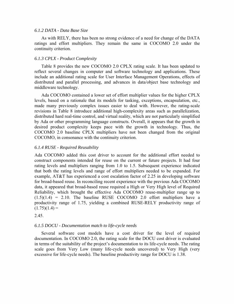
6.1.2 DATA - Data Base Size

As with RELY, there has been no strong evidence of a need for change of the DATA ratings and effort multipliers. They remain the same in COCOMO 2.0 under the continuity criterion.

6.1.3 CPLX - Product Complexity

Table 8 provides the new COCOMO 2.0 CPLX rating scale. It has been updated to reflect several changes in computer and software technology and applications. These include an additional rating scale for User Interface Management Operations, effects of distributed and parallel processing, and advances in data/object base technology and middleware technology.

Ada COCOMO contained a lower set of effort multiplier values for the higher CPLX levels, based on a rationale that its models for tasking, exceptions, encapsulation, etc., made many previously complex issues easier to deal with. However, the rating-scale revisions in Table 8 introduce additional high-complexity areas such as parallelization, distributed hard real-time control, and virtual reality, which are not particularly simplified by Ada or other programming language constructs. Overall, it appears that the growth in desired product complexity keeps pace with the growth in technology. Thus, the COCOMO 2.0 baseline CPLX multipliers have not been changed from the original COCOMO, in consonance with the continuity criterion.

6.1.4 RUSE - Required Reusability

Ada COCOMO added this cost driver to account for the additional effort needed to construct components intended for reuse on the current or future projects. It had four rating levels and multipliers ranging from 1.0 to 1.5. Subsequent experience indicated that both the rating levels and range of effort multipliers needed to be expanded. For example, AT&T has experienced a cost escalation factor of 2.25 in developing software for broad-based reuse. In reconciling recent experience with the previous Ada COCOMO data, it appeared that broad-based reuse required a High or Very High level of Required Reliability, which brought the effective Ada COCOMO reuse-multiplier range up to (1.5)(1.4) = 2.10. The baseline RUSE COCOMO 2.0 effort multipliers have a productivity range of 1.75, yielding a combined RUSE-RELY productivity range of (1.75)(1.4) =

2.45.

6.1.5 DOCU - Documentation match to life-cycle needs

Several software cost models have a cost driver for the level of required documentation. In COCOMO 2.0, the rating scale for the DOCU cost driver is evaluated in terms of the suitability of the project’s documentation to its life-cycle needs. The rating scale goes from Very Low (many life-cycle needs uncovered) to Very High (very excessive for life-cycle needs). The baseline productivity range for DOCU is 1.38.

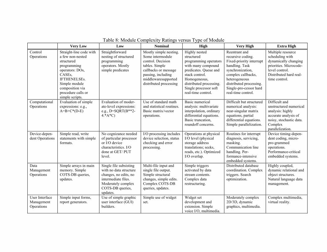
Table 8: Module Complexity Ratings versus Type of Module Very Low Low Nominal High Very High Extra High Control Operations

Straight-line code with a few non-nested structured programming operators: DOs, CASEs, IFTHENELSEs. Simple module composition via procedure calls or simple scripts.

Straightforward nesting of structured programming operators. Mostly simple predicates

Mostly simple nesting. Some intermodule control. Decision tables. Simple callbacks or message passing, including middlewaresupported distributed processing

Highly nested structured programming operators with many compound predicates. Queue and stack control. Homogeneous, distributed processing. Single processor soft real-time control.

Reentrant and recursive coding. Fixed-priority interrupt handling. Task synchronization, complex callbacks, heterogeneous distributed processing. Single-pro-cessor hard real-time control.

Multiple resource scheduling with dynamically changing priorities. Microcode-level control. Distributed hard real-time control.

Computational Operations

Evaluation of simple expressions: e.g., A=B+C*(D-E)

Evaluation of moder-ate-level expressions: e.g., D=SQRT(B**2-4.*A*C)

Use of standard math and statistical routines. Basic matrix/vector operations.

Basic numerical analysis: multivariate interpolation, ordinary differential equations. Basic truncation, roundoff concerns.

Difficult but structured numerical analysis: near-singular matrix equations, partial differential equations. Simple parallelization.

Difficult and unstructured numerical analysis: highly accurate analysis of noisy, stochastic data. Complex parallelization.

Device-depen-dent Operations

Simple read, write statements with simple formats.

No cognizance needed of particular processor or I/O device characteristics. I/O done at GET/ PUT level.

I/O processing includes device selection, status checking and error processing.

Operations at physical I/O level (physical storage address translations; seeks, reads, etc.). Optimized I/O overlap.

Routines for interrupt diagnosis, servicing, masking. Communication line handling. Per-formance-intensive embedded systems.

Device timing-depen-dent coding, micro-pro-grammed operations. Performance-critical embedded systems.

Data Management Operations

Simple arrays in main memory. Simple COTS-DB queries, updates.

Single file subsisting with no data structure changes, no edits, no intermediate files. Moderately complex COTS-DB queries, updates.

Multi-file input and single file output. Simple structural changes, simple edits. Complex COTS-DB queries, updates.

Simple triggers activated by data stream contents. Complex data restructuring.

Distributed database coordination. Complex triggers. Search optimization.

Highly coupled, dynamic relational and object structures. Natural language data management.

User Interface Management Operations

Simple input forms, report generators.

Use of simple graphic user interface (GUI) builders.

Simple use of widget set.

Widget set development and extension. Simple voice I/O, multimedia.

Moderately complex 2D/3D, dynamic graphics, multimedia.

Complex multimedia, virtual reality.

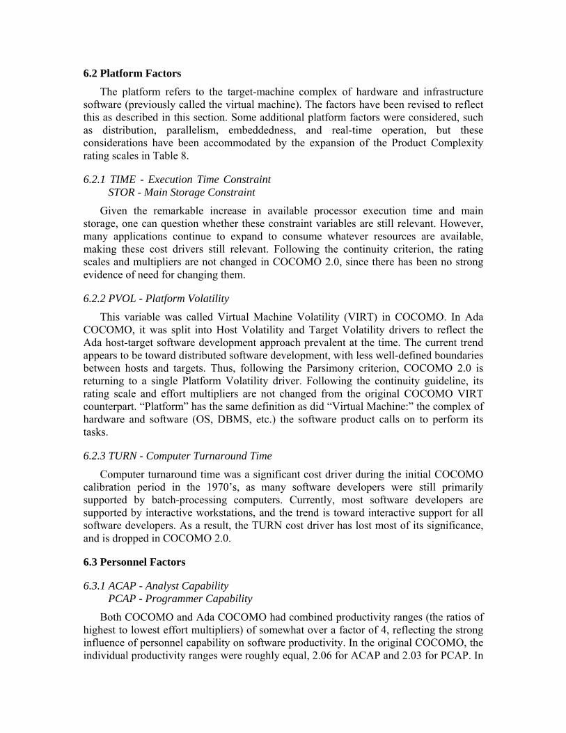
6.2 Platform Factors

The platform refers to the target-machine complex of hardware and infrastructure software (previously called the virtual machine). The factors have been revised to reflect this as described in this section. Some additional platform factors were considered, such as distribution, parallelism, embeddedness, and real-time operation, but these considerations have been accommodated by the expansion of the Product Complexity rating scales in Table 8.

6.2.1 TIME - Execution Time Constraint STOR - Main Storage Constraint

Given the remarkable increase in available processor execution time and main storage, one can question whether these constraint variables are still relevant. However, many applications continue to expand to consume whatever resources are available, making these cost drivers still relevant. Following the continuity criterion, the rating scales and multipliers are not changed in COCOMO 2.0, since there has been no strong evidence of need for changing them.

6.2.2 PVOL - Platform Volatility

This variable was called Virtual Machine Volatility (VIRT) in COCOMO. In Ada COCOMO, it was split into Host Volatility and Target Volatility drivers to reflect the Ada host-target software development approach prevalent at the time. The current trend appears to be toward distributed software development, with less well-defined boundaries between hosts and targets. Thus, following the Parsimony criterion, COCOMO 2.0 is returning to a single Platform Volatility driver. Following the continuity guideline, its rating scale and effort multipliers are not changed from the original COCOMO VIRT counterpart. “Platform” has the same definition as did “Virtual Machine:” the complex of hardware and software (OS, DBMS, etc.) the software product calls on to perform its tasks.

6.2.3 TURN - Computer Turnaround Time

Computer turnaround time was a significant cost driver during the initial COCOMO calibration period in the 1970’s, as many software developers were still primarily supported by batch-processing computers. Currently, most software developers are supported by interactive workstations, and the trend is toward interactive support for all software developers. As a result, the TURN cost driver has lost most of its significance, and is dropped in COCOMO 2.0.

6.3 Personnel Factors

6.3.1 ACAP - Analyst Capability PCAP - Programmer Capability

Both COCOMO and Ada COCOMO had combined productivity ranges (the ratios of highest to lowest effort multipliers) of somewhat over a factor of 4, reflecting the strong influence of personnel capability on software productivity. In the original COCOMO, the individual productivity ranges were roughly equal, 2.06 for ACAP and 2.03 for PCAP. In

Ada COCOMO, the Ada Process Model was organized around a small number of good analysts producing a definitive specification to be implemented by generally less-capable programmers. This led to a higher productivity range, 2.57, for ACAP, as compared to 1.62 for PCAP.

Current trends continue to emphasize the importance of highly capable analysts. However the increasing role of complex COTS packages, and the significant productivity leverage associated with programmers’ ability to deal with these COTS packages, indicates a trend toward higher importance of programmer capability as well.

For these reasons the COCOMO 2.0 baseline effort multipliers for ACAP and PCAP maintain the same composite productivity range, but provide an intermediate position with respect to the relative productivity ranges of ACAP and PCAP. The resulting baseline COCOMO 2.0 effort multipliers have productivity ranges of 2.24 for ACAP and 1.85 for PCAP.

6.3.2 AEXP - Applications Experience PEXP - Platform Experience LTEX - Language and Tool Experience

COCOMO 2.0 makes three primary changes in these three personnel experience cost drivers:

• Transforming them to a common rating scale, to avoid some previous confusion;

• Broadening the productivity influence of PEXP, recognizing the importance of understanding the use of more powerful platforms, including more graphic user interface, database, networking, and distributed middleware capabilities;

• Extending the previous Language Experience cost driver to include experience with software tools and methods.

The resulting baseline COCOMO 2.0 effort multipliers for these cost drivers have the following comparative effect on previous COCOMO productivity ranges:

• AEXP: 1.54 in COCOMO 2.0 versus 1.57 in COCOMO and Ada COCOMO

• PEXP: 1.58 in COCOMO 2.0 versus 1.34 in COCOMO and Ada COCOMO (VEXP)

• LTEX: 1.51 in COCOMO 2.0 versus 1.20 in COCOMO and Ada COCOMO (LEXP)

6.3.3 PCON - Personnel Continuity

The original COCOMO data collection and analysis included a potential PCON cost driver, but the analysis results were inconclusive and the cost driver was not included [Boehm 1981, p.486-487]. The COCOMO 2.0 rating scale for PCON is in terms of the project’s annual personnel turnover: from 3% to 48%. The corresponding baseline productivity range is 1.52.

6.4 Project Factors

6.4.1 MODP - Use of Modern Programming Practices

The definition of “modern programming practices” has evolved into a broader “mature software engineering practices” term exemplified by the Software Engineering Institute Capability maturity Model [Paulk et al 1993] and comparable models such as ISO 9000-3 and SPICE. The cost estimation effects of this broader set of practices are addressed in COCOMO 2.0 via the Process Maturity exponent driver. As a result, the MODP effort-multiplier cost driver has been dropped.

6.4.2 TOOL - Use of Software Tools

Software tools have improved significantly since the 1970’s projects used to calibrate COCOMO. Ada COCOMO added two rating levels to address late-1980’s and expected 1990’s tool capabilities. Since then, the number of projects with COCOMO TOOL ratings of Very Low and Low have become scarce. Therefore, COCOMO 2.0 has shifted the TOOL scale to eliminate the original Very Low and Low levels and to use an updated interpretation of the upper five Ada COCOMO rating levels as the TOOL scale. The elimination of two rating levels between Ada COCOMO and COCOMO 2.0 reduced the productivity range from 2.00 to 1.61.

6.4.3 SITE - Multisite Development

Given the increasing frequency of multisite developments, and indications from COCOMO users and from other cost models that multisite development effects are significant, the SITE cost driver has been added in COCOMO 2.0. Determining its cost driver rating involves the assessment and averaging of two factors: site collocation (from fully collocated to international distribution) and communication support (from surface mail and some phone access to full interactive multimedia). The corresponding baseline productivity range is 1.57.

6.4.4 SCED - Required Development Schedule

Given that there has been no strong evidence of a need to change the SCED ratings and effort multipliers, they remain the same in the baseline COCOMO 2.0 under the continuity criterion.

6.4.5 SECU - Classified Security Application

Ada COCOMO included a SECU cost driver, which applied an effort multiplier of 1.10 of a project required classified security procedures. Using the parsimony criterion, since most projects do not need to deal with this, we have dropped it from COCOMO 2.0

7. Additional COCOMO 2.0 Capabilities This section covers the remainder of the initial COCOMO 2.0 capabilities: Early

Design and Post-Architecture estimation models using Function Points; schedule estimation, and output estimate ranges. Further COCOMO 2.0 capabilities, such as the effects of reuse and applications composition on phase and activity distribution of effort and schedule, will be covered in future papers.

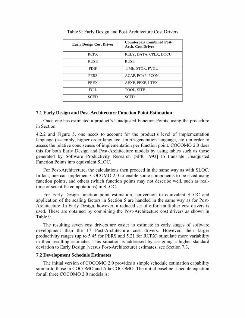
Table 9: Early Design and Post-Architecture Cost Drivers

Early Design Cost Driver Counterpart Combined Post-Arch. Cost Driver

RCPX RELY, DATA, CPLX, DOCU

RUSE RUSE

PDIF TIME, STOR, PVOL

PERS ACAP, PCAP, PCON

PREX AEXP, PEXP, LTEX

FCIL TOOL, SITE

SCED SCED

7.1 Early Design and Post-Architecture Function Point Estimation

Once one has estimated a product’s Unadjusted Function Points, using the procedure in Section

4.2.2 and Figure 5, one needs to account for the product’s level of implementation language (assembly, higher order language, fourth-generation language, etc.) in order to assess the relative conciseness of implementation per function point. COCOMO 2.0 does this for both Early Design and Post-Architecture models by using tables such as those generated by Software Productivity Research [SPR 1993] to translate Unadjusted Function Points into equivalent SLOC.

For Post-Architecture, the calculations then proceed in the same way as with SLOC. In fact, one can implement COCOMO 2.0 to enable some components to be sized using function points, and others (which function points may not describe well, such as real-time or scientific computations) in SLOC.

For Early Design function point estimation, conversion to equivalent SLOC and application of the scaling factors in Section 5 are handled in the same way as for Post-Architecture. In Early Design, however, a reduced set of effort multiplier cost drivers is used. These are obtained by combining the Post-Architecture cost drivers as shown in Table 9.

The resulting seven cost drivers are easier to estimate in early stages of software development than the 17 Post-Architecture cost drivers. However, their larger productivity ranges (up to 5.45 for PERS and 5.21 for RCPX) stimulate more variability in their resulting estimates. This situation is addressed by assigning a higher standard deviation to Early Design (versus Post-Architecture) estimates; see Section 7.3.

7.2 Development Schedule Estimates

The initial version of COCOMO 2.0 provides a simple schedule estimation capability similar to those in COCOMO and Ada COCOMO. The initial baseline schedule equation for all three COCOMO 2.0 models is:

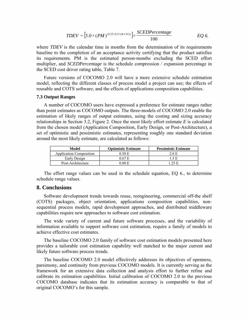
[ ]100

×)(×0.3= ))01.1-(×2.0+33.0( tageSCEDPercenPMTDEV B EQ 6.

where TDEV is the calendar time in months from the determination of its requirements baseline to the completion of an acceptance activity certifying that the product satisfies its requirements. PM is the estimated person-months excluding the SCED effort multiplier, and SCEDPercentage is the schedule compression / expansion percentage in the SCED cost driver rating table, Table 7.

Future versions of COCOMO 2.0 will have a more extensive schedule estimation model, reflecting the different classes of process model a project can use; the effects of reusable and COTS software; and the effects of applications composition capabilities.

7.3 Output Ranges

A number of COCOMO users have expressed a preference for estimate ranges rather than point estimates as COCOMO outputs. The three-models of COCOMO 2.0 enable the estimation of likely ranges of output estimates, using the costing and sizing accuracy relationships in Section 3.2, Figure 2. Once the most likely effort estimate E is calculated from the chosen model (Application Composition, Early Design, or Post-Architecture), a set of optimistic and pessimistic estimates, representing roughly one standard deviation around the most likely estimate, are calculated as follows:

Model Optimistic Estimate Pessimistic Estimate Application Composition 0.50 E 2.0 E

Early Design 0.67 E 1.5 E Post-Architecture 0.80 E 1.25 E

The effort range values can be used in the schedule equation, EQ 6., to determine schedule range values.

8. Conclusions Software development trends towards reuse, reengineering, commercial off-the shelf

(COTS) packages, object orientation, applications composition capabilities, non-sequential process models, rapid development approaches, and distributed middleware capabilities require new approaches to software cost estimation.

The wide variety of current and future software processes, and the variability of information available to support software cost estimation, require a family of models to achieve effective cost estimates.

The baseline COCOMO 2.0 family of software cost estimation models presented here provides a tailorable cost estimation capability well matched to the major current and likely future software process trends.

The baseline COCOMO 2.0 model effectively addresses its objectives of openness, parsimony, and continuity from previous COCOMO models. It is currently serving as the framework for an extensive data collection and analysis effort to further refine and calibrate its estimation capabilities. Initial calibration of COCOMO 2.0 to the previous COCOMO database indicates that its estimation accuracy is comparable to that of original COCOMO’s for this sample.

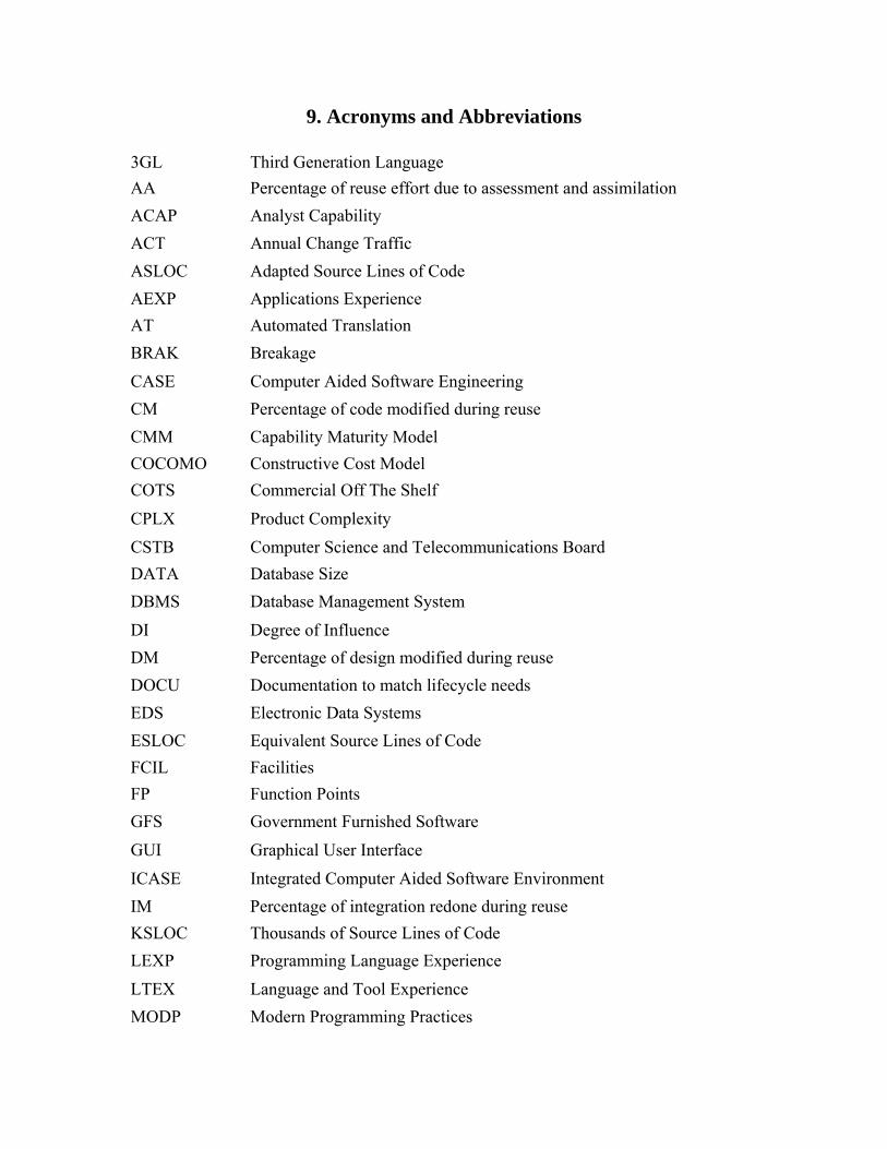
9. Acronyms and Abbreviations

3GL Third Generation Language AA Percentage of reuse effort due to assessment and assimilation ACAP Analyst Capability ACT Annual Change Traffic ASLOC Adapted Source Lines of Code AEXP Applications Experience AT Automated Translation BRAK Breakage CASE Computer Aided Software Engineering CM Percentage of code modified during reuse CMM Capability Maturity Model COCOMO Constructive Cost Model COTS Commercial Off The Shelf CPLX Product Complexity CSTB Computer Science and Telecommunications Board DATA Database Size DBMS Database Management System DI Degree of Influence DM Percentage of design modified during reuse DOCU Documentation to match lifecycle needs EDS Electronic Data Systems ESLOC Equivalent Source Lines of Code FCIL Facilities FP Function Points GFS Government Furnished Software GUI Graphical User Interface ICASE Integrated Computer Aided Software Environment IM Percentage of integration redone during reuse KSLOC Thousands of Source Lines of Code LEXP Programming Language Experience LTEX Language and Tool Experience MODP Modern Programming Practices

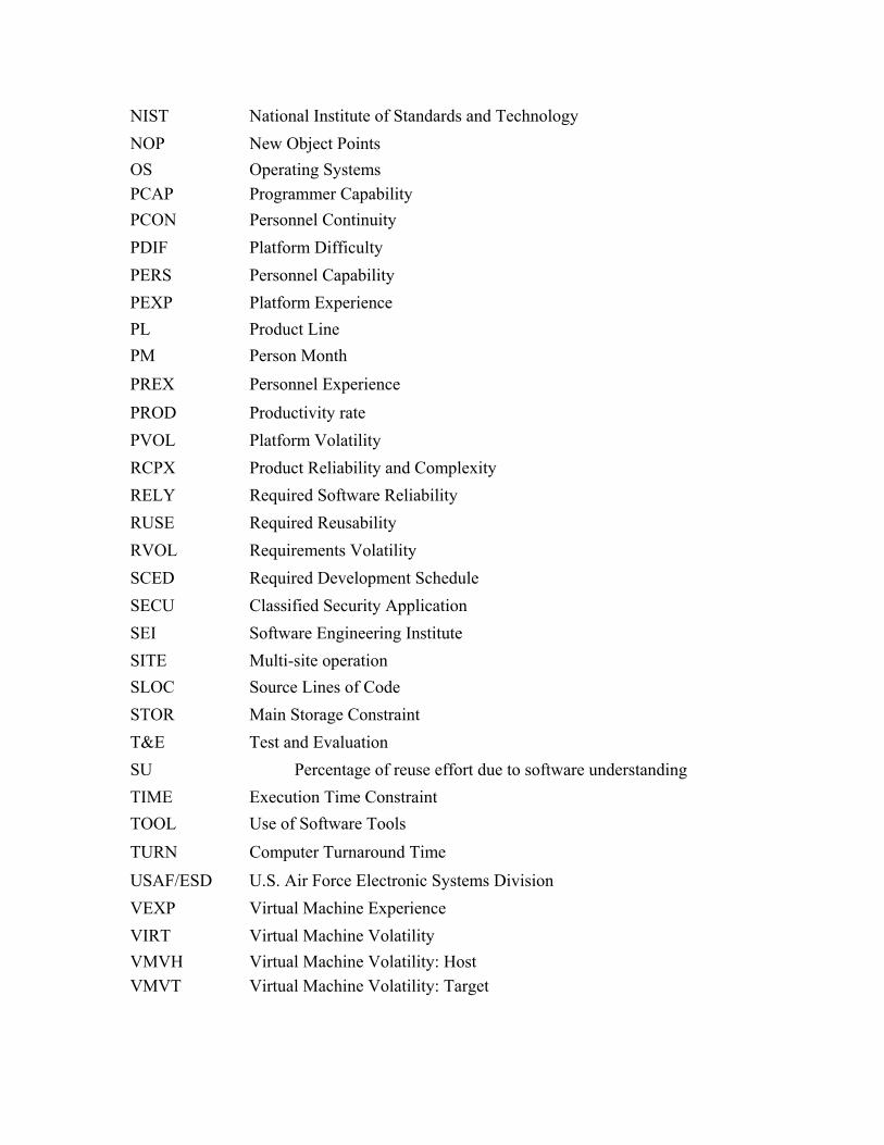
NIST National Institute of Standards and Technology NOP New Object Points OS Operating Systems PCAP Programmer Capability PCON Personnel Continuity PDIF Platform Difficulty PERS Personnel Capability PEXP Platform Experience PL Product Line PM Person Month

PREX Personnel Experience

PROD Productivity rate PVOL Platform Volatility RCPX Product Reliability and Complexity RELY Required Software Reliability RUSE Required Reusability RVOL Requirements Volatility SCED Required Development Schedule SECU Classified Security Application SEI Software Engineering Institute SITE Multi-site operation SLOC Source Lines of Code STOR Main Storage Constraint T&E Test and Evaluation SU Percentage of reuse effort due to software understanding TIME Execution Time Constraint TOOL Use of Software Tools TURN Computer Turnaround Time

USAF/ESD U.S. Air Force Electronic Systems Division VEXP Virtual Machine Experience VIRT Virtual Machine Volatility VMVH Virtual Machine Volatility: Host VMVT Virtual Machine Volatility: Target

10. Acknowledgments This work has been supported both financially and technically by the COCOMO 2.0

Program Affiliates: Aerospace, AT&T Bell Labs, Bellcore, DISA, EDS, E-Systems, Hewlett-Packard, Hughes, IDA, IDE, JPL, Litton Data Systems, Lockheed, Loral, MDAC, Motorola, Northrop, Rational, Rockwell, SAIC, SEI, SPC, TASC, Teledyne, TI, TRW, USAF Rome Lab, US Army Research Lab, Xerox.

11. References Amadeus (1994), Amadeus Measurement System User’s Guide, Version 2.3a, Amadeus

Software Research, Inc., Irvine, California, July 1994.

Banker, R., R. Kauffman and R. Kumar (1994), “An Empirical Test of Object-Based Output Measurement Metrics in a Computer Aided Software Engineering (CASE) Environment,” Journal of Management Information Systems (to appear, 1994).

Banker, R., H. Chang and C. Kemerer (1994a), “Evidence on Economies of Scale in Software Development,” Information and Software Technology (to appear, 1994).

Behrens, C. (1983), “Measuring the Productivity of Computer Systems Development Activities with Function Points,” IEEE Transactions on Software Engineering, November 1983.

Boehm, B. (1981), Software Engineering Economics, Prentice Hall.

Boehm, B. (1983), “The Hardware/Software Cost Ratio: Is It a Myth?” Computer 16(3), March 1983, pp. 78-80.

Boehm, B. (1985), “COCOMO: Answering the Most Frequent Questions,” In Proceedings, First COCOMO Users’ Group Meeting, Wang Institute, Tyngsboro, MA, May 1985.

Boehm, B. (1989), Software Risk Management, IEEE Computer Society Press, Los Alamitos, CA.

Boehm, B., T. Gray, and T. Seewaldt (1984), “Prototyping vs. Specifying: A Multi-Project Experiment,” IEEE Transactions on Software Engineering, May 1984, pp. 133-145.

Boehm, B., and W. Royce (1989), “Ada COCOMO and the Ada Process Model,” Proceedings, Fifth COCOMO Users’ Group Meeting, Software Engineering Institute, Pittsburgh, PA, November 1989.

Chidamber, S. and C. Kemerer (1994), “A Metrics Suite for Object Oriented Design,” IEEE Transactions on Software Engineering, (to appear 1994).

Computer Science and Telecommunications Board (CSTB) National Research Council (1993), Computing Professionals: Changing Needs for the 1990’s, National Academy Press, Washington DC, 1993.

Devenny, T. (1976). “An Exploratory Study of Software Cost Estimating at the Electronic Systems Division,” Thesis No. GSM/SM/765-4, Air Force Institute of Technology, Dayton, OH.

Gerlich, R., and U. Denskat (1994), “A Cost Estimation Model for Maintenance and High Reuse,” Proceedings, ESCOM 1994, Ivrea, Italy.

Goethert, W., E. Bailey, M. Busby (1992), “Software Effort and Schedule Measurement: A Framework for Counting Staff Hours and Reporting Schedule Information.” CMU/SEI-92-TR-21, Software Engineering Institute, Pittsburgh, PA.

Goudy, R. (1987), “COCOMO-Based Personnel Requirements Model,” Proceedings, Third COCOMO Users’ Group Meeting, Software Engineering Institute, Pittsburgh, PA, November 1987.

IFPUG (1994), IFPUG Function Point Counting Practices: Manual Release 4.0, International Function Point Users’ Group, Westerville, OH.

Kauffman, R., and R. Kumar (1993), “Modeling Estimation Expertise in Object Based ICASE Environments,” Stern School of Business Report, New York University, January 1993.

Kemerer, C. (1987), “An Empirical Validation of Software Cost Estimation Models,” Communications of the ACM, May 1987, pp. 416-429.

Kominski, R. (1991), Computer Use in the United States: 1989, Current Population Reports, Series

P-23, No. 171, U.S. Bureau of the Census, Washington, D.C., February 1991.

Kunkler, J. (1983), “A Cooperative Industry Study on Software Development/Maintenance Productivity,” Xerox Corporation, Xerox Square --- XRX2 52A, Rochester, NY 14644, Third Report, March 1985.

Miyazaki, Y., and K. Mori (1985), “COCOMO Evaluation and Tailoring,” Proceedings, ICSE 8, IEEE-ACM-BCS, London, August 1985, pp. 292-299.

Parikh, G., and N. Zvegintzov (1983). “The World of Software Maintenance,” Tutorial on Software Maintenance, IEEE Computer Society Press, pp. 1-3.

Park R. (1992), “Software Size Measurement: A Framework for Counting Source Statements.” CMU/SEI-92-TR-20, Software Engineering Institute, Pittsburgh, PA.

Park R, W. Goethert, J. Webb (1994), “Software Cost and Schedule Estimating: A Process Improvement Initiative”, CMU/SEI-94-SR-03, Software Engineering Institute, Pittsburgh, PA.

Paulk, M., B. Curtis, M. Chrissis, and C. Weber (1993), “Capability Maturity Model for Software, Version 1.1”, CMU-SEI-93-TR-24, Software Engineering Institute, Pittsburgh PA 15213.

Pfleeger, S. (1991), “Model of Software Effort and Productivity,” Information and Software Technology 33 (3), April 1991, pp. 224-231.

Royce, W. (1990), “TRW’s Ada Process Model for Incremental Development of Large Software Systems,” Proceedings, ICSE 12, Nice, France, March 1990.

Ruhl, M., and M. Gunn (1991), “Software Reengineering: A Case Study and Lessons Learned,” NIST Special Publication 500-193, Washington, DC, September 1991.

Selby, R. (1988), “Empirically Analyzing Software Reuse in a Production Environment,” In Software Reuse: Emerging Technology, W. Tracz (Ed.), IEEE Computer Society Press, 1988., pp. 176-189.

Selby, R., A. Porter, D. Schmidt and J. Berney (1991), “Metric-Driven Analysis and Feedback Systems for Enabling Empirically Guided Software Development,” Proceedings of the Thirteenth International Conference on Software Engineering (ICSE 13), Austin, TX, May 1316, 1991, pp. 288-298.

Silvestri, G. and J. Lukaseiwicz (1991), “Occupational Employment Projections,” Monthly Labor Review 114(11), November 1991, pp. 64-94.

SPR (1993), “Checkpoint User’s Guide for the Evaluator”, Software Productivity Research, Inc., Burlington, MA., 1993.