Embed Size (px)
Citation preview
Cost Minimization and Cost CurvesEcon 212 Lecture 12
Tianyi Wang
Queen’s Univeristy
Winter 2013
Tianyi Wang (Queen’s Univeristy) Costs Winter 2013 1 / 37
Introduction
I We want to model how firms make use of technologies.I Take as given the objective of firms: profit maximization.I One period problem, no risks.I Opportunity cost, sunk cost and fixed cost.I Start with Cost Minimization, for
I itself is interesting.I can not max profit without minimize cost
I Profit = Revenue - Cost = P ∗Q − C (Q)I Suppost cost not minimized for a set of inputs, given Q , can inproveprofit by reducing cost.
Tianyi Wang (Queen’s Univeristy) Costs Winter 2013 2 / 37
Cost Minimization in Long-run
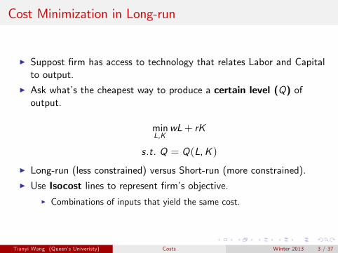
I Suppost firm has access to technology that relates Labor and Capitalto output.
I Ask what’s the cheapest way to produce a certain level (Q) ofoutput.
minL,K
wL+ rK
s.t. Q = Q(L,K )
I Long-run (less constrained) versus Short-run (more constrained).I Use Isocost lines to represent firm’s objective.
I Combinations of inputs that yield the same cost.
Tianyi Wang (Queen’s Univeristy) Costs Winter 2013 3 / 37

Figure: Isocost Line
Tianyi Wang (Queen’s Univeristy) Costs Winter 2013 4 / 37
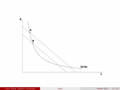
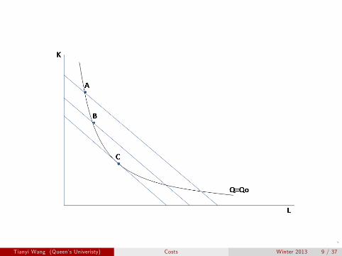
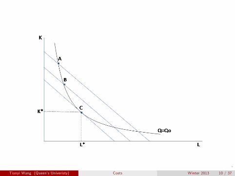
Optimal Input Choices
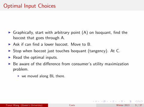
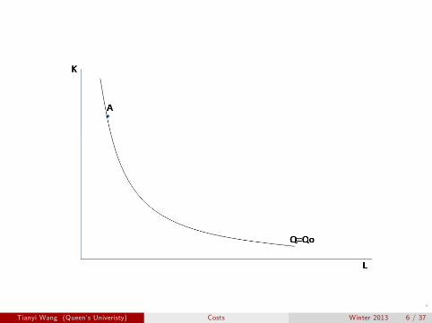
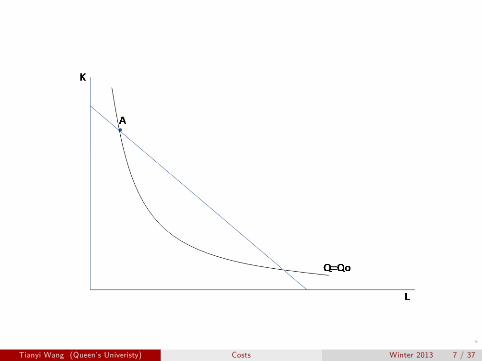
I Graphically, start with arbitrary point (A) on Isoquant, find theIsocost that goes through A.
I Ask if can find a lower Isocost. Move to B.I Stop when Isocost just touches Isoquant (tangency). At C.I Read the optimal inputs.I Be aware of the difference from consumer’s utility maximizationproblem.
I we moved along BL there.
Tianyi Wang (Queen’s Univeristy) Costs Winter 2013 5 / 37
Tianyi Wang (Queen’s Univeristy) Costs Winter 2013 6 / 37
Tianyi Wang (Queen’s Univeristy) Costs Winter 2013 7 / 37
Tianyi Wang (Queen’s Univeristy) Costs Winter 2013 8 / 37
Tianyi Wang (Queen’s Univeristy) Costs Winter 2013 9 / 37
Tianyi Wang (Queen’s Univeristy) Costs Winter 2013 10 / 37
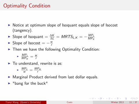
Optimality Condition
I Notice at optimum slope of Isoquant equals slope of Isocost(tangency).
I Slope of Isoquant = ∆K∆L = MRTSL,K = − MPL
MPKI Slope of Isocost = −wrI Then we have the following Optimality Condition:
I MPLMPK
= wr
I To understand, rewrite is as:I MPL
w = MPKr
I Marginal Product derived from last dollar equals.I "bang for the buck"
Tianyi Wang (Queen’s Univeristy) Costs Winter 2013 11 / 37
Optimality Condition (Con’t)
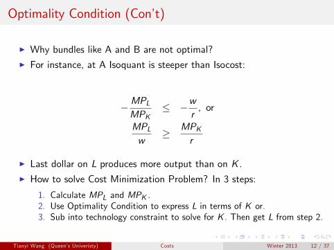
I Why bundles like A and B are not optimal?I For instance, at A Isoquant is steeper than Isocost:
−MPLMPK
≤ −wr, or
MPLw
≥ MPKr
I Last dollar on L produces more output than on K .I How to solve Cost Minimization Problem? In 3 steps:
1. Calculate MPL and MPK .2. Use Optimality Condition to express L in terms of K or.3. Sub into technology constraint to solve for K . Then get L from step 2.
Tianyi Wang (Queen’s Univeristy) Costs Winter 2013 12 / 37
Optimality Condition (Con’t)
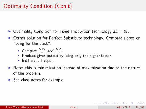
I Optimality Condition for Fixed Proportion technology aL = bK .I Corner solution for Perfect Substitute technology. Compare slopes or"bang for the buck".
I Compare MPLw and MPKr .
I Produce given output by using only the higher factor.I Indifferent if equal.
I Note: this is minimization instead of maximization due to the natureof the problem.
I See class notes for example.
Tianyi Wang (Queen’s Univeristy) Costs Winter 2013 13 / 37
Comparative Statics
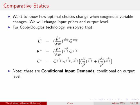
I Want to know how optimal choices change when exogenous variablechanges. We will change input prices and output level.
I For Cobb-Douglas technology, we solved that:
L∗ = (βrαw)
αα+βQ
1α+β
K ∗ = (βrαw)−β
α+βQ1
α+β
C ∗ = Q1
α+βwβ
α+β rα
α+β [(α
β)−α
α+β + (α
β)−β
α+β ]
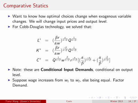
I Note: these are Conditional Input Demands, conditional on outputlevel.
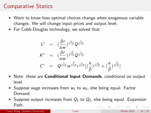
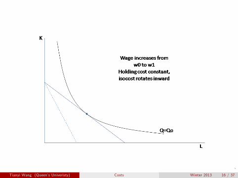
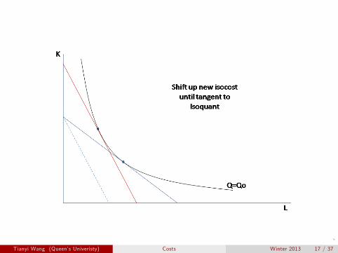
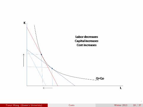
I Suppose wage increases from w1 to w2, else being equal. FactorDemand.
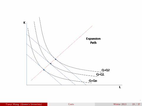
I Suppose output increases from Q1 to Q2, else being equal. ExpansionPath.
Tianyi Wang (Queen’s Univeristy) Costs Winter 2013 14 / 37
Comparative Statics
I Want to know how optimal choices change when exogenous variablechanges. We will change input prices and output level.
I For Cobb-Douglas technology, we solved that:
L∗ = (βrαw)
αα+βQ
1α+β
K ∗ = (βrαw)−β
α+βQ1
α+β
C ∗ = Q1
α+βwβ
α+β rα
α+β [(α
β)−α
α+β + (α
β)−β
α+β ]
I Note: these are Conditional Input Demands, conditional on outputlevel.
I Suppose wage increases from w1 to w2, else being equal. FactorDemand.
I Suppose output increases from Q1 to Q2, else being equal. ExpansionPath.
Tianyi Wang (Queen’s Univeristy) Costs Winter 2013 14 / 37
Comparative Statics
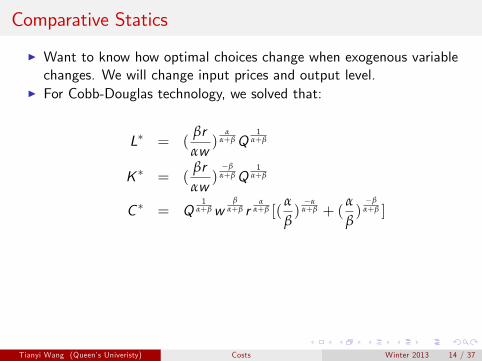
I Want to know how optimal choices change when exogenous variablechanges. We will change input prices and output level.
I For Cobb-Douglas technology, we solved that:
L∗ = (βrαw)
αα+βQ
1α+β
K ∗ = (βrαw)−β
α+βQ1
α+β
C ∗ = Q1
α+βwβ
α+β rα
α+β [(α
β)−α
α+β + (α
β)−β
α+β ]
I Note: these are Conditional Input Demands, conditional on outputlevel.
I Suppose wage increases from w1 to w2, else being equal. FactorDemand.
I Suppose output increases from Q1 to Q2, else being equal. ExpansionPath.
Tianyi Wang (Queen’s Univeristy) Costs Winter 2013 14 / 37
Tianyi Wang (Queen’s Univeristy) Costs Winter 2013 15 / 37
Tianyi Wang (Queen’s Univeristy) Costs Winter 2013 16 / 37
Tianyi Wang (Queen’s Univeristy) Costs Winter 2013 17 / 37
Tianyi Wang (Queen’s Univeristy) Costs Winter 2013 18 / 37
Tianyi Wang (Queen’s Univeristy) Costs Winter 2013 19 / 37
Input Demands
I We can vary wages to get optimal labor demands. Downward sloping.
I We can vary rental rates to get optimal capital demands. Downwardsloping.
I See class notes for graphs.
I Price elasticity of demand ε =∆LL
∆ww= dL
dwwL
Tianyi Wang (Queen’s Univeristy) Costs Winter 2013 20 / 37
Input Demands
I We can vary wages to get optimal labor demands. Downward sloping.I We can vary rental rates to get optimal capital demands. Downwardsloping.
I See class notes for graphs.
I Price elasticity of demand ε =∆LL
∆ww= dL
dwwL
Tianyi Wang (Queen’s Univeristy) Costs Winter 2013 20 / 37
Input Demands
I We can vary wages to get optimal labor demands. Downward sloping.I We can vary rental rates to get optimal capital demands. Downwardsloping.
I See class notes for graphs.
I Price elasticity of demand ε =∆LL
∆ww= dL
dwwL
Tianyi Wang (Queen’s Univeristy) Costs Winter 2013 20 / 37
Input Demands
I We can vary wages to get optimal labor demands. Downward sloping.I We can vary rental rates to get optimal capital demands. Downwardsloping.
I See class notes for graphs.
I Price elasticity of demand ε =∆LL
∆ww= dL
dwwL
Tianyi Wang (Queen’s Univeristy) Costs Winter 2013 20 / 37
Cost Minimization in Short-run
I In the short-run, capital is fixed at some predetermined level, firm’sproblem becomes,
Cs (Q, K̄ ) = minLwL+ r K̄
s.t. Q = Q(L, K̄ )
I Simple: constraint determines optimal amount of Labor.I Note long-run cost can be written as C (Q) = Cs (Q,K ∗(Q))
I LR cost equals SR cost when capital is fixed at the optimal level.
Tianyi Wang (Queen’s Univeristy) Costs Winter 2013 21 / 37
Cost Curve in Short-run
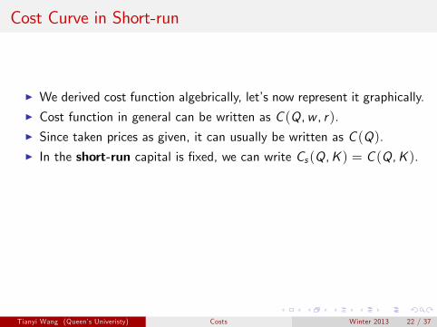
I We derived cost function algebrically, let’s now represent it graphically.
I Cost function in general can be written as C (Q,w , r).I Since taken prices as given, it can usually be written as C (Q).I In the short-run capital is fixed, we can write Cs (Q,K ) = C (Q,K ).I Note some costs depend on output others not.
I C (Q,K ) = Cv (Q,K )︸ ︷︷ ︸+ F︸︷︷︸Varaible Fixed
I See class note for graph
Tianyi Wang (Queen’s Univeristy) Costs Winter 2013 22 / 37
Cost Curve in Short-run
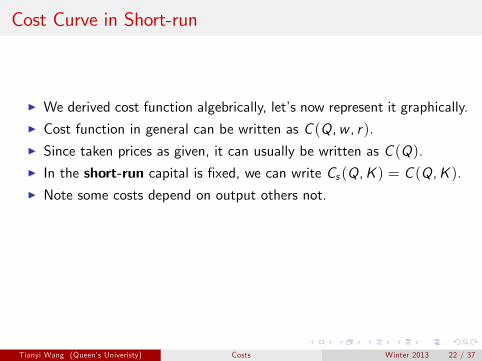
I We derived cost function algebrically, let’s now represent it graphically.I Cost function in general can be written as C (Q,w , r).
I Since taken prices as given, it can usually be written as C (Q).I In the short-run capital is fixed, we can write Cs (Q,K ) = C (Q,K ).I Note some costs depend on output others not.
I C (Q,K ) = Cv (Q,K )︸ ︷︷ ︸+ F︸︷︷︸Varaible Fixed
I See class note for graph
Tianyi Wang (Queen’s Univeristy) Costs Winter 2013 22 / 37
Cost Curve in Short-run
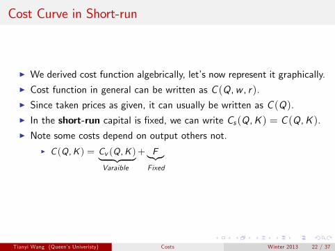
I We derived cost function algebrically, let’s now represent it graphically.I Cost function in general can be written as C (Q,w , r).I Since taken prices as given, it can usually be written as C (Q).
I In the short-run capital is fixed, we can write Cs (Q,K ) = C (Q,K ).I Note some costs depend on output others not.
I C (Q,K ) = Cv (Q,K )︸ ︷︷ ︸+ F︸︷︷︸Varaible Fixed
I See class note for graph
Tianyi Wang (Queen’s Univeristy) Costs Winter 2013 22 / 37
Cost Curve in Short-run
I We derived cost function algebrically, let’s now represent it graphically.I Cost function in general can be written as C (Q,w , r).I Since taken prices as given, it can usually be written as C (Q).I In the short-run capital is fixed, we can write Cs (Q,K ) = C (Q,K ).
I Note some costs depend on output others not.
I C (Q,K ) = Cv (Q,K )︸ ︷︷ ︸+ F︸︷︷︸Varaible Fixed
I See class note for graph
Tianyi Wang (Queen’s Univeristy) Costs Winter 2013 22 / 37
Cost Curve in Short-run
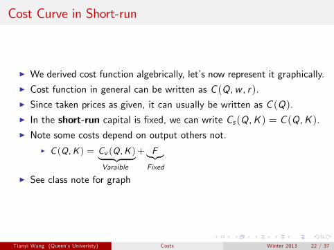
I We derived cost function algebrically, let’s now represent it graphically.I Cost function in general can be written as C (Q,w , r).I Since taken prices as given, it can usually be written as C (Q).I In the short-run capital is fixed, we can write Cs (Q,K ) = C (Q,K ).I Note some costs depend on output others not.
I C (Q,K ) = Cv (Q,K )︸ ︷︷ ︸+ F︸︷︷︸Varaible Fixed
I See class note for graph
Tianyi Wang (Queen’s Univeristy) Costs Winter 2013 22 / 37
Cost Curve in Short-run
I We derived cost function algebrically, let’s now represent it graphically.I Cost function in general can be written as C (Q,w , r).I Since taken prices as given, it can usually be written as C (Q).I In the short-run capital is fixed, we can write Cs (Q,K ) = C (Q,K ).I Note some costs depend on output others not.
I C (Q,K ) = Cv (Q,K )︸ ︷︷ ︸+ F︸︷︷︸Varaible Fixed
I See class note for graph
Tianyi Wang (Queen’s Univeristy) Costs Winter 2013 22 / 37
Average Cost Curve
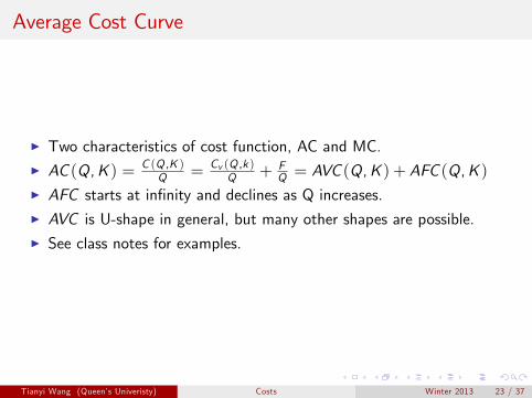
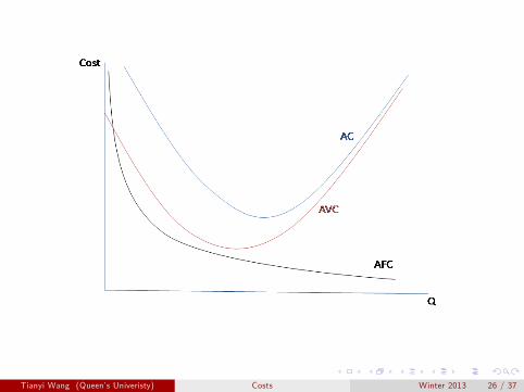
I Two characteristics of cost function, AC and MC.
I AC (Q,K ) = C (Q ,K )Q = Cv (Q ,k )
Q + FQ = AVC (Q,K ) + AFC (Q,K )
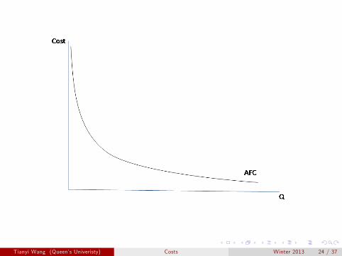
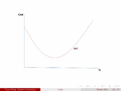
I AFC starts at infinity and declines as Q increases.I AVC is U-shape in general, but many other shapes are possible.I See class notes for examples.
Tianyi Wang (Queen’s Univeristy) Costs Winter 2013 23 / 37
Average Cost Curve
I Two characteristics of cost function, AC and MC.I AC (Q,K ) = C (Q ,K )
Q = Cv (Q ,k )Q + F
Q = AVC (Q,K ) + AFC (Q,K )
I AFC starts at infinity and declines as Q increases.I AVC is U-shape in general, but many other shapes are possible.I See class notes for examples.
Tianyi Wang (Queen’s Univeristy) Costs Winter 2013 23 / 37
Average Cost Curve
I Two characteristics of cost function, AC and MC.I AC (Q,K ) = C (Q ,K )
Q = Cv (Q ,k )Q + F
Q = AVC (Q,K ) + AFC (Q,K )I AFC starts at infinity and declines as Q increases.
I AVC is U-shape in general, but many other shapes are possible.I See class notes for examples.
Tianyi Wang (Queen’s Univeristy) Costs Winter 2013 23 / 37
Average Cost Curve
I Two characteristics of cost function, AC and MC.I AC (Q,K ) = C (Q ,K )
Q = Cv (Q ,k )Q + F
Q = AVC (Q,K ) + AFC (Q,K )I AFC starts at infinity and declines as Q increases.I AVC is U-shape in general, but many other shapes are possible.
I See class notes for examples.
Tianyi Wang (Queen’s Univeristy) Costs Winter 2013 23 / 37
Average Cost Curve
I Two characteristics of cost function, AC and MC.I AC (Q,K ) = C (Q ,K )
Q = Cv (Q ,k )Q + F
Q = AVC (Q,K ) + AFC (Q,K )I AFC starts at infinity and declines as Q increases.I AVC is U-shape in general, but many other shapes are possible.I See class notes for examples.
Tianyi Wang (Queen’s Univeristy) Costs Winter 2013 23 / 37
Tianyi Wang (Queen’s Univeristy) Costs Winter 2013 24 / 37
Tianyi Wang (Queen’s Univeristy) Costs Winter 2013 25 / 37
Tianyi Wang (Queen’s Univeristy) Costs Winter 2013 26 / 37
Marginal Cost Curve
I MC (Q,K ) = ∆C (Q ,K )∆Q = C ′(Q,K )
I Note MC (Q,K ) = C ′(Q,K ) = C ′v (Q, k) + F′ = C ′v (Q, k)
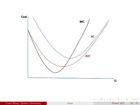
I Relationship b/w MC and AVC
I MC of the first unit is the same as the AVC of that unit.I When AVC decreases, MC must be less than AVC.I When AVC increases, MC must be greater than AVC.I MC intersects AVC at the minimum of AVC.
I Similar relationship b/w MC and AC.
Tianyi Wang (Queen’s Univeristy) Costs Winter 2013 27 / 37
Marginal Cost Curve
I MC (Q,K ) = ∆C (Q ,K )∆Q = C ′(Q,K )
I Note MC (Q,K ) = C ′(Q,K ) = C ′v (Q, k) + F′ = C ′v (Q, k)
I Relationship b/w MC and AVCI MC of the first unit is the same as the AVC of that unit.
I When AVC decreases, MC must be less than AVC.I When AVC increases, MC must be greater than AVC.I MC intersects AVC at the minimum of AVC.
I Similar relationship b/w MC and AC.
Tianyi Wang (Queen’s Univeristy) Costs Winter 2013 27 / 37

Marginal Cost Curve
I MC (Q,K ) = ∆C (Q ,K )∆Q = C ′(Q,K )
I Note MC (Q,K ) = C ′(Q,K ) = C ′v (Q, k) + F′ = C ′v (Q, k)
I Relationship b/w MC and AVCI MC of the first unit is the same as the AVC of that unit.I When AVC decreases, MC must be less than AVC.
I When AVC increases, MC must be greater than AVC.I MC intersects AVC at the minimum of AVC.
I Similar relationship b/w MC and AC.
Tianyi Wang (Queen’s Univeristy) Costs Winter 2013 27 / 37
Marginal Cost Curve
I MC (Q,K ) = ∆C (Q ,K )∆Q = C ′(Q,K )
I Note MC (Q,K ) = C ′(Q,K ) = C ′v (Q, k) + F′ = C ′v (Q, k)
I Relationship b/w MC and AVCI MC of the first unit is the same as the AVC of that unit.I When AVC decreases, MC must be less than AVC.I When AVC increases, MC must be greater than AVC.
I MC intersects AVC at the minimum of AVC.
I Similar relationship b/w MC and AC.
Tianyi Wang (Queen’s Univeristy) Costs Winter 2013 27 / 37
Marginal Cost Curve
I MC (Q,K ) = ∆C (Q ,K )∆Q = C ′(Q,K )
I Note MC (Q,K ) = C ′(Q,K ) = C ′v (Q, k) + F′ = C ′v (Q, k)
I Relationship b/w MC and AVCI MC of the first unit is the same as the AVC of that unit.I When AVC decreases, MC must be less than AVC.I When AVC increases, MC must be greater than AVC.I MC intersects AVC at the minimum of AVC.
I Similar relationship b/w MC and AC.
Tianyi Wang (Queen’s Univeristy) Costs Winter 2013 27 / 37
Tianyi Wang (Queen’s Univeristy) Costs Winter 2013 28 / 37
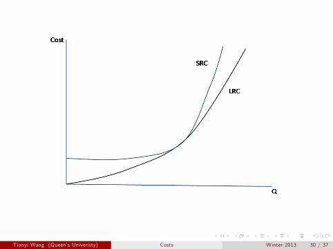
Cost curves in the Long-run
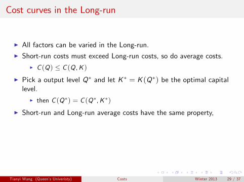
I All factors can be varied in the Long-run.
I Short-run costs must exceed Long-run costs, so do average costs.
I C (Q) ≤ C (Q,K )
I Pick a output level Q∗ and let K ∗ = K (Q∗) be the optimal capitallevel.
I then C (Q∗) = C (Q∗,K ∗)
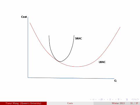
I Short-run and Long-run average costs have the same property,
I AC (Q) ≤ AC (Q,K ∗)I AC (Q∗) = AC (Q∗,K ∗)
I short-run curves always lie above long-run curve except for one point.
Tianyi Wang (Queen’s Univeristy) Costs Winter 2013 29 / 37
Cost curves in the Long-run
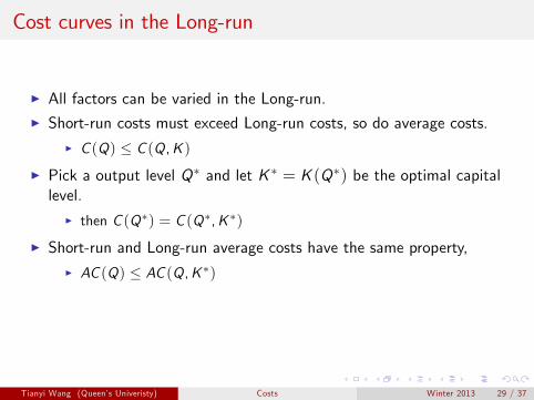
I All factors can be varied in the Long-run.I Short-run costs must exceed Long-run costs, so do average costs.
I C (Q) ≤ C (Q,K )I Pick a output level Q∗ and let K ∗ = K (Q∗) be the optimal capitallevel.
I then C (Q∗) = C (Q∗,K ∗)
I Short-run and Long-run average costs have the same property,
I AC (Q) ≤ AC (Q,K ∗)I AC (Q∗) = AC (Q∗,K ∗)
I short-run curves always lie above long-run curve except for one point.
Tianyi Wang (Queen’s Univeristy) Costs Winter 2013 29 / 37
Cost curves in the Long-run
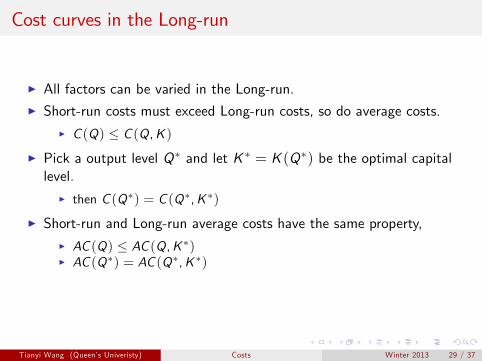
I All factors can be varied in the Long-run.I Short-run costs must exceed Long-run costs, so do average costs.
I C (Q) ≤ C (Q,K )
I Pick a output level Q∗ and let K ∗ = K (Q∗) be the optimal capitallevel.
I then C (Q∗) = C (Q∗,K ∗)
I Short-run and Long-run average costs have the same property,
I AC (Q) ≤ AC (Q,K ∗)I AC (Q∗) = AC (Q∗,K ∗)
I short-run curves always lie above long-run curve except for one point.
Tianyi Wang (Queen’s Univeristy) Costs Winter 2013 29 / 37
Cost curves in the Long-run
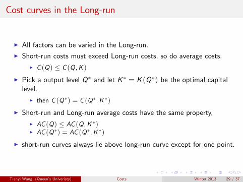
I All factors can be varied in the Long-run.I Short-run costs must exceed Long-run costs, so do average costs.
I C (Q) ≤ C (Q,K )I Pick a output level Q∗ and let K ∗ = K (Q∗) be the optimal capitallevel.
I then C (Q∗) = C (Q∗,K ∗)
I Short-run and Long-run average costs have the same property,
I AC (Q) ≤ AC (Q,K ∗)I AC (Q∗) = AC (Q∗,K ∗)
I short-run curves always lie above long-run curve except for one point.
Tianyi Wang (Queen’s Univeristy) Costs Winter 2013 29 / 37

Cost curves in the Long-run
I All factors can be varied in the Long-run.I Short-run costs must exceed Long-run costs, so do average costs.
I C (Q) ≤ C (Q,K )I Pick a output level Q∗ and let K ∗ = K (Q∗) be the optimal capitallevel.
I then C (Q∗) = C (Q∗,K ∗)
I Short-run and Long-run average costs have the same property,
I AC (Q) ≤ AC (Q,K ∗)I AC (Q∗) = AC (Q∗,K ∗)
I short-run curves always lie above long-run curve except for one point.
Tianyi Wang (Queen’s Univeristy) Costs Winter 2013 29 / 37
Cost curves in the Long-run
I All factors can be varied in the Long-run.I Short-run costs must exceed Long-run costs, so do average costs.
I C (Q) ≤ C (Q,K )I Pick a output level Q∗ and let K ∗ = K (Q∗) be the optimal capitallevel.
I then C (Q∗) = C (Q∗,K ∗)
I Short-run and Long-run average costs have the same property,I AC (Q) ≤ AC (Q,K ∗)
I AC (Q∗) = AC (Q∗,K ∗)
I short-run curves always lie above long-run curve except for one point.
Tianyi Wang (Queen’s Univeristy) Costs Winter 2013 29 / 37
Cost curves in the Long-run
I All factors can be varied in the Long-run.I Short-run costs must exceed Long-run costs, so do average costs.
I C (Q) ≤ C (Q,K )I Pick a output level Q∗ and let K ∗ = K (Q∗) be the optimal capitallevel.
I then C (Q∗) = C (Q∗,K ∗)
I Short-run and Long-run average costs have the same property,I AC (Q) ≤ AC (Q,K ∗)I AC (Q∗) = AC (Q∗,K ∗)
I short-run curves always lie above long-run curve except for one point.
Tianyi Wang (Queen’s Univeristy) Costs Winter 2013 29 / 37
Tianyi Wang (Queen’s Univeristy) Costs Winter 2013 30 / 37
Tianyi Wang (Queen’s Univeristy) Costs Winter 2013 31 / 37
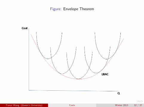
Figure: Envelope Theorem
Tianyi Wang (Queen’s Univeristy) Costs Winter 2013 32 / 37

Long-Run Marginal Costs
I Long-run marginal cost curve of any output level has to equal theshort-run marginal cost curve associated with the optimal level ofplant size to produce that level of output.
I This is known as the Envelope Theorem
Tianyi Wang (Queen’s Univeristy) Costs Winter 2013 33 / 37
Long-Run Marginal Costs
I Long-run marginal cost curve of any output level has to equal theshort-run marginal cost curve associated with the optimal level ofplant size to produce that level of output.
I This is known as the Envelope Theorem
Tianyi Wang (Queen’s Univeristy) Costs Winter 2013 33 / 37
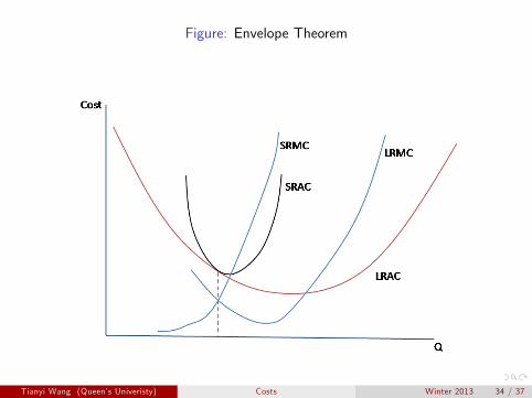
Figure: Envelope Theorem
Tianyi Wang (Queen’s Univeristy) Costs Winter 2013 34 / 37
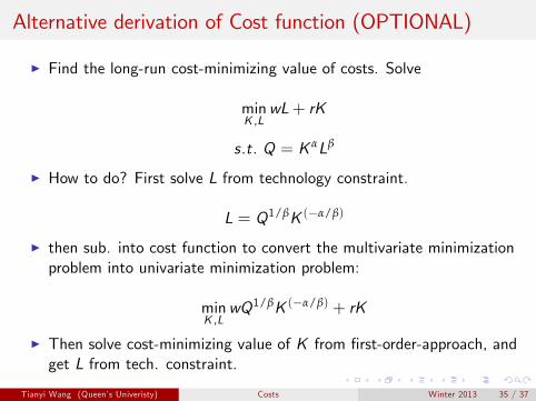
Alternative derivation of Cost function (OPTIONAL)
I Find the long-run cost-minimizing value of costs. Solve
minK ,L
wL+ rK
s.t. Q = K αLβ
I How to do? First solve L from technology constraint.
L = Q1/βK (−α/β)
I then sub. into cost function to convert the multivariate minimizationproblem into univariate minimization problem:
minK ,L
wQ1/βK (−α/β) + rK
I Then solve cost-minimizing value of K from first-order-approach, andget L from tech. constraint.
Tianyi Wang (Queen’s Univeristy) Costs Winter 2013 35 / 37
Alternative derivation of Cost function (Con’t)
I Note it is similar as fixing K in step 1 and find the optimal L for agiven value of capital, then sets capital equal to the value that wouldhave been chosen if it had not been fixed.
I This is short-run cost computed at the optimal capital level!I So, long-run cost equals the short-run cost determined at the’appropriate’capital stock
Tianyi Wang (Queen’s Univeristy) Costs Winter 2013 36 / 37
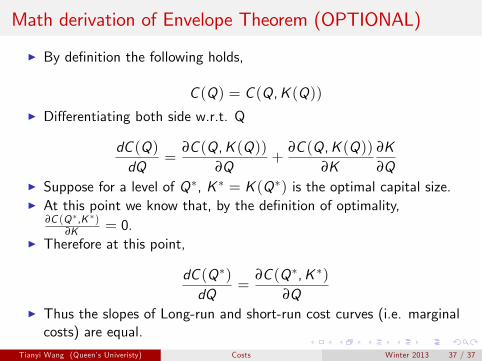
Math derivation of Envelope Theorem (OPTIONAL)
I By definition the following holds,
C (Q) = C (Q,K (Q))
I Differentiating both side w.r.t. Q
dC (Q)dQ
=∂C (Q,K (Q))
∂Q+
∂C (Q,K (Q))∂K
∂K∂Q
I Suppose for a level of Q∗, K ∗ = K (Q∗) is the optimal capital size.I At this point we know that, by the definition of optimality,
∂C (Q ∗,K ∗)∂K = 0.
I Therefore at this point,
dC (Q∗)dQ
=∂C (Q∗,K ∗)
∂QI Thus the slopes of Long-run and short-run cost curves (i.e. marginalcosts) are equal.
Tianyi Wang (Queen’s Univeristy) Costs Winter 2013 37 / 37