Embed Size (px)
Citation preview

Cost Evaluation of North Sea
Offshore Wind Post 2030
On behalf of the North Sea Wind Power Hub Consortium
4 February 2019

Project Cost Evaluation of North Sea Offshore Wind Post 2030
Client North Sea Wind Power Hub Consortium
Document
Status Final
Date 4 February 2019
Reference 112522/19-001.830
Project code 112522
Project Leader K.A. Haans MSc
Project Director M.T. Marshall MTech
Author(s) E.C.M. Ruijgrok PhD, E.J. van Druten MSc, B.H. Bulder MSc (ECN part of TNO)
Checked by A.H.J. van Kuijk MSc
Approved by K.A. Haans MSc
Initials
Address Witteveen+Bos Raadgevende ingenieurs B.V.
Leeuwenbrug 8
P.O. Box 233
7400 AE Deventer
The Netherlands
+31 570 69 79 11
www.witteveenbos.com
CoC 38020751
The Quality management system of Witteveen+Bos has been approved based on ISO 9001.
© Witteveen+Bos
No part of this document may be reproduced and/or published in any form, without prior written permission of Witteveen+Bos, and the NSWPH
consortium, nor may it be used for any work other than that for which it was manufactured without such permission, unless otherwise agreed in
writing. Witteveen+Bos, ECN part of TNO and the NSWPH consortium do not accept liability for damages or loss arising from application or use of any
outcome of the content of this document.
TABLE OF CONTENTS
1 INTRODUCTION 20
1.1 Background 20
1.2 Study purpose 21
1.3 Reading guide 21
2 FINDING SPACE FOR OFFSHORE WIND ENERGY IN THE NORTH SEA 23
2.1 Space consumption in the North Sea 23
2.2 Optimizing grid connection design by cooperation between countries 25
2.3 Cost drivers and optimal use of economies of scale 26
3 STARTING POINTS 27
3.1 Study scope 27
3.1.1 Methodological scope 27 3.1.2 Geographical and depth scope 28 3.1.3 Roll-out scope 29 3.1.4 Cost scope 29
3.2 Trends in of offshore wind energy production 30
3.3 Reference wind farm and grid connection for this study 32
3.4 Used input data 33
4 LCOE-R MAPPING MODEL 35
4.1 LCoE mapping 35
4.1.1 LCoE formula 35 4.1.2 OWF cost formulas 37 4.1.3 GCS cost formulas 39 4.1.4 LCoE uncertainty margins 41 4.1.5 LCoE maps 43
4.2 LCoE-R mapping 45
4.2.1 Spatial risk principles 45 4.2.2 LCoE-R calculations 48 4.2.3 LCoE-R maps 52

5 IDENTIFYING POSSIBLE NEW OWF LOCATIONS 56
5.1 Searching for new locations from different perspectives 56
5.1.1 Set with possible new locations based on low LCoE-R 56 5.1.2 Set with possible new locations excluding visibility from shore 57 5.1.3 Set with possible new locations excluding nature protected areas 58
5.2 Selection of a preferred set with possible new locations for grid roll-out 59
6 GRID ROLL-OUT PATHWAYS 62
6.1 Adding inter-OWF wake losses 62
6.2 Grid optimization and economies of scale 63
6.3 Identified roll-out pathways 65
6.3.1 Pathway 1: Enough hubs 66 6.3.2 Pathway 2: Large hubs 67 6.3.3 Capturing economies of scale 68
6.4 Selection of preferred grid roll-out pathway 69
7 SENSITIVITY ANALYSES 70
7.1 Sensitivity to wind farm power density 70
7.2 Sensitivity to no hubs 72
7.3 Sensitivity to including areas just outside nature areas 73
8 MAIN RESULTS & FOLLOW UP STUDIES 77
8.1 Main results 77
8.1.1 Possible new OWF locations and their LCoEs 77 8.1.2 Roll-out pathways and their LCoE 78 8.1.3 Sensitivity analyses 78
8.2 Follow-up studies 79
8.2.1 More detailed investigation of spatial risks 79 8.2.2 Economies and diseconomies of scale 80 8.2.3 Include interconnection benefits 80
9 REFERENCES 81
Last page 82

APPENDICES Number of
pages
I Trends in space use at the North Sea 10
II Spatial cost calculation formulas 2
III Detailed design of German shipping corridors 3

7 | 82 Witteveen+Bos | 112522/19-001.830 | Final report
LIST OF USED ABBREVIATIONS
- AC Alternating Current
- AC farm Offshore wind farm that is connected with an AC radial grid connection system
- AEP Annual Energy Production
- CapEx Capital Expenditure
- COP21 21st Conference of the Parties in Paris
- DC Direct Current
- DC farm Offshore wind farm that is connected with a DC radial grid connection system
- EEZ Exclusive Economic Zone
- GCS Grid Connection System
- GIS Geographic Information System
- GW Gigawatt
- H&S Hub and Spoke
- H&S farm Offshore wind farm that is connected with a H&S grid connection system
- LCoE Levelized Cost of Energy
- LCoE-R Levelized Cost of Energy including spatial Risk
- MW Megawatt
- MWh Megawatt hour
- NM Nautical Mile
- NSWPH North Sea Wind Power Hub
- O&M Operation and Maintenance
- OpEx Operational Expenditure
- OWF Offshore Wind Farm
- TWh Terawatt hour
- WSI Wind farm Sensitivity Index

8 | 82 Witteveen+Bos | 112522/19-001.830 | Final report
SUMMARY
Decarbonizing electricity production
Meeting the climate change targets of the Paris Agreement is a challenge that involves deployment of large
scale offshore wind energy production capacity. Recent estimates show that approximately 180 GW of
offshore wind capacity is required in the North Sea to decarbonize the power sector of the North Sea
Declaration countries1.
The North Sea countries2 have planned new OWF capacity of 55 GW up to 2030 and 20 GW3 after 2030. This
study looks into the OWF locations post 2030. Taking into account the planned capacity up until 2030, an
additional 110 GW is expected to be needed.
Finding space for wind farms in a heavily used sea
The North Sea is used for many different purposes, such as shipping, military exercises, fisheries and sand
mining. Figure S1 (left) shows the present space consumption of the various users of the North Sea.
Figure S1 (right) shows the remaining suitable space (water depth ≤ 55 m) when excluding areas used by
other functions.
Figure S1 Present space consumption (left); Remaining space (depth ≤ 55 m) when using an exclusionary approach (right)
On the basis of these maps it was calculated that only approximately 3 % of the suitable space4 remains
available for OWFs (14,000 km2), if all the used areas are excluded. The remaining space can host 47-84 GW,
depending on the used power density5. This is less than the strived for 110 GW. It leads to the observation
that a co-utilization approach will be necessary in the future6. The extent to which co-utilization will be
needed highly depends on future developments such as the decommissioning of oil and gas platforms.
Identifying possible new OWF locations with relatively low cost
Policy makers consider multiple criteria when identifying and selecting new offshore wind farm locations.
These criteria include techno-economic considerations (such as water depth, wind speed, cost and subsidies),
1 By Muller et al. (2017).
2 Including Norway, the UK, the Netherlands and the North Sea EEZs of Denmark and Germany.
3 When expressed in terms of the power density of 3.6 MW/km2, which is used in this study.
4 Percentage of the study area, which is the North Sea with a depth ≤ 55 meter, minus the EEZ of Belgium and France.
5 3.6-6.4 MW/km2 . 6 In addition to or as an alternative to an exclusionary approach.
9 | 82 Witteveen+Bos | 112522/19-001.830 | Final report
existing spatial claims, the natural environment and public concerns such as visibility. Considering these
criteria, the objectives of this study are to:
1 identify possible new locations in the North Sea region where OWFs can be developed without excluding
areas used by other functions beforehand;
2 calculate the levelized cost of energy (LCoE) of these locations;
3 take the risk of encountering other user functions into account by means of a first evaluation of the cost
of co-utilization (LCoE-R), i.e. the cost of mutual adaptation of user functions and OWFs to each other’s
presence at sea;
4 design grid roll-out pathways to connect the identified new locations to the onshore grid that combine
all available grid connection types (AC, DC and H&S);
5 discover connected OWF-clusters with a relatively low overall LCoE.
The study provides a basis from which the NSWPH consortium can contribute to the general discussion on
North Sea spatial planning by providing insight into offshore wind energy production and transmission costs
for different locations across the North Sea.
Study scope and key assumptions
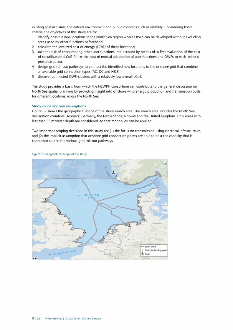
Figure S2 shows the geographical scope of the study search area. The search area includes the North Sea
declaration countries Denmark, Germany, the Netherlands, Norway and the United Kingdom. Only areas with
less than 55 m water depth are considered, so that monopiles can be applied.
Two important scoping decisions in this study are (1) the focus on transmission using electrical infrastructure,
and (2) the implicit assumption that onshore grid connection points are able to host the capacity that is
connected to it in the various grid roll-out pathways.
Figure S2 Geographical scope of the study

10 | 82 Witteveen+Bos | 112522/19-001.830 | Final report
Reference wind farm
Considering the trend of increasing turbine size and wind farm size, this study uses a 1 GW reference farm
for the future that contains 67 turbines (monopiles) of 15 MW. A power density of 3.6 MW/km2 is used,
based on the expectation of ECN part of TNO that this is an optimal future density with an eye on inter-OWF
(i.e. OWF cluster) wake losses.
Grid connection systems
Three different grid connection systems are used in this study: AC radial, DC radial and hub and spoke (H&S)
(see figure S3). AC radial is used for farms nearshore (up to 80 km). DC radial is used for isolated farms far
from shore (more than 80 km). H&S is applied to clusters of farms far from shore (more than 80 km).
The hubs of the H&S are located within OWF clusters in such a way that each hub can serve as many OWFs
as possible. Farms at a distance up to 30 km of a hub are connected to the hub with 66 kV AC inter-array
cables. In order to also connect farms at distances up to 80 km of a hub, an extra AC substation is used that
is connected to the hub with 220 kV AC cables. The latter is called ‘AC hybrid’.
Figure S3 Grid connection systems applied in study
North Sea covering mapping tool
In this study a mapping tool is developed that calculates and visualises the levelized cost of energy of all grid
cells7 of the North Sea. The tool allows its user to draw new wind farms on the basis of this cost information
and to connect them to existing onshore landing points with the grid connection systems AC radial, DC
radial and/or the relatively new concept of H&S. Table S1 presents the data used in the mapping tool.
7 The size of a grid cell is 1/48 degree in longitude and latitude, which is approximately 310 hectares..
11 | 82 Witteveen+Bos | 112522/19-001.830 | Final report
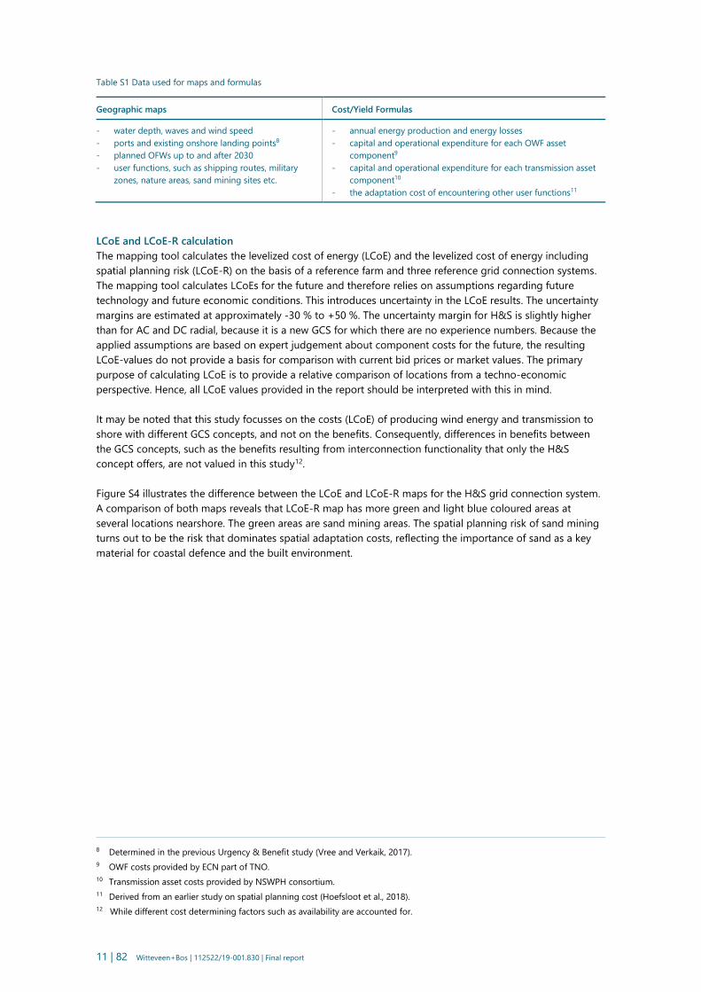
Table S1 Data used for maps and formulas
Geographic maps Cost/Yield Formulas
- water depth, waves and wind speed
- ports and existing onshore landing points8
- planned OFWs up to and after 2030
- user functions, such as shipping routes, military
zones, nature areas, sand mining sites etc.
- annual energy production and energy losses
- capital and operational expenditure for each OWF asset
component9
- capital and operational expenditure for each transmission asset
component10
- the adaptation cost of encountering other user functions11
LCoE and LCoE-R calculation
The mapping tool calculates the levelized cost of energy (LCoE) and the levelized cost of energy including
spatial planning risk (LCoE-R) on the basis of a reference farm and three reference grid connection systems.
The mapping tool calculates LCoEs for the future and therefore relies on assumptions regarding future
technology and future economic conditions. This introduces uncertainty in the LCoE results. The uncertainty
margins are estimated at approximately -30 % to +50 %. The uncertainty margin for H&S is slightly higher
than for AC and DC radial, because it is a new GCS for which there are no experience numbers. Because the
applied assumptions are based on expert judgement about component costs for the future, the resulting
LCoE-values do not provide a basis for comparison with current bid prices or market values. The primary
purpose of calculating LCoE is to provide a relative comparison of locations from a techno-economic
perspective. Hence, all LCoE values provided in the report should be interpreted with this in mind.
It may be noted that this study focusses on the costs (LCoE) of producing wind energy and transmission to
shore with different GCS concepts, and not on the benefits. Consequently, differences in benefits between
the GCS concepts, such as the benefits resulting from interconnection functionality that only the H&S
concept offers, are not valued in this study12.
Figure S4 illustrates the difference between the LCoE and LCoE-R maps for the H&S grid connection system.
A comparison of both maps reveals that LCoE-R map has more green and light blue coloured areas at
several locations nearshore. The green areas are sand mining areas. The spatial planning risk of sand mining
turns out to be the risk that dominates spatial adaptation costs, reflecting the importance of sand as a key
material for coastal defence and the built environment.
8 Determined in the previous Urgency & Benefit study (Vree and Verkaik, 2017).
9 OWF costs provided by ECN part of TNO.
10 Transmission asset costs provided by NSWPH consortium.
11 Derived from an earlier study on spatial planning cost (Hoefsloot et al., 2018).
12 While different cost determining factors such as availability are accounted for.

12 | 82 Witteveen+Bos | 112522/19-001.830 | Final report
Figure S4 LCoE (top) and LCoE-R (bottom) maps for the H&S grid connection system
The LCoE is calculated on the basis of the capital and operational expenditure of the OWF and GCS and the
annual energy production (see figure S4). Future onshore grid reinforcement costs are not included in the
GCS expenditures13. As a first approximation for minimising grid integration cost, deeper inland connections
have been considered. These connect offshore transmission cables to locations where available connection
capacity is expected based on fossil fuel phase-out scenarios.
13 These costs are deeply uncertain. Since the energy transition requires significant grid reinforcements anyhow, it is questionable
whether these costs should be included in the LCoE of offshore wind. A special onshore grid connection study is required to
determine these costs, which is outside the scope of this study.

13 | 82 Witteveen+Bos | 112522/19-001.830 | Final report
In order to determine the yearly CapEx, the total CapEx over the lifespan of the OWF is divided by an annuity
of 20. This annuity is based on a 30 year lifespan plus a discount rate of 2.9 %. The annual energy production
corrected for both availability (96-97 %) and the energy losses (1.0-1.2 %) of the OWF and GCS.
Figure S5 LCoE and LCoE-R calculation
The LCoE-R is calculated in a similar way as the LCoE, but it also includes spatial planning risks (see
figure S5). Instead of excluding locations that are already used by other functions, the risk of encountering
other functions is expressed in terms of adaptation costs. This renders locations that are intensively used by
other functions more expensive than those that are not.
Adaptation costs are determined in terms of the cost for adapting the wind farm to the user function or vice
versa. For example, in nature areas the wind farms adapt by means of shutting down turbines when birds fly
over and/or by applying ‘Building with Nature’ solutions e.g. scour protection that stimulates reef builder
species. For minor shipping routes, the shipping function adapts by sailing around the wind farm, while for
major routes, the farm layout is adapted by creating a shipping corridor through the farm. All these
adaptations lead to costs which are roughly estimated and included in the LCoE-R maps. These estimates
add to the uncertainty range of the LCoE-R and therefore accentuate the need to interpret the values from a
relative comparison perspective and not their absolute value.
Though adaptation costs of multiple users at one location are included in the LCoE-R, the cumulative costs
caused by the presence of multiple OWFs in the North Sea, i.e. of OWF clusters, are not accounted for14.
The magnitude of these cumulative costs is not known at this time and difficult to estimate. It is therefore
not possible to indicate the impact cumulative costs would have on the LCOE-R.
Searching for possible new locations from different perspectives
On the basis of the LCoE-R maps possible new OWF locations were identified from three different
perspectives:
- low LCoE-R;
- visibility from shore;
- nature conservation.
14 In this study, the purpose was to let spatial adaptation cost influence the identification of new possible locations. Cumulative
adaptation costs of OWF clusters can, however, only be calculated after the selection of a set of new locations.

14 | 82 Witteveen+Bos | 112522/19-001.830 | Final report
Table S2 presents the key characteristics of the three sets of possible new locations and of the baseline farms
that have been planned up to and after 2030. This table shows that the average LCoEs of the three sets of
possible new locations range from 37 to 39 €/MWh, while the average LCoE-R is slightly higher and ranges
from 38 to 40 €/MWh. The overall adaptation costs for OWF locations overlapping with existing functions
can be calculated by the difference between the average LCoE and LCoE-R of the roll-out list and is
approximately 0.6 €/MWh.
Table S2 Key features of the baseline and the three set with possible new locations
Set with possible new locations Number of
OWF
Surface (km2) Capacity (3.6
MW/km2)
(GW)
LCoE
(€/MWh)
LCoE-R
(€/MWh)
Baseline up to 2030 99 13,000 55* - -
Baseline planned after 2030 24 5,000 20** 39 40
LCOE-R based set 113 31,000 110 37 38
Visibility based set 130 34,000 120 37 38
Nature based set 87 21,000 77 38 38
OWF roll-out list after 2030 =
Baseline planned after 2030 +
LCOE-R based set
137 36,000 130 37 38
* The power density of these OWFs deviates from the power density of the reference farm which is 3.6 MW/km2.
** This capacity is recalculated for a power density of 3.6 MW/km2 ; see appendix I, table I.1.
Table S2 also reveals that the set with possible new locations that excludes nature areas has a lower capacity
than strived for (77 GW instead of 110 GW15). A sensitivity analysis in this study looked at the impact on
the overall LCoE by adding OWF locations to compensate for the insufficient capacity level of this set .
A more detailed inspection of the cost numbers disclosed that the LCoE-R based set is economically the
most attractive one. Together with the planned baseline locations for the period after 2030 it was therefore
selected as a roll-out list, for which grid roll-out pathways are designed. Figure S6 shows this roll-out list.
15 An extra amount of 110 GW is expected to be needed after 2030 to meet the COP21 target to decarbonize the power sector of
the North Sea Declaration countries.

15 | 82 Witteveen+Bos | 112522/19-001.830 | Final report
Figure S6 Roll-out list
Designing grid roll-out pathways
For the roll-out list of figure S6, two grid roll-out pathways were designed, following two different
approaches:
- a simple roll-out approach, with enough hubs to connect all OWFs. This approach optimized the hub
location, taking into account the 66 kV cable reach of 30 km. This roll-out path contains 17 hubs with a
capacity ranging from 3 to 8 GW (see figure S7 left);
- a more complex roll-out approach, where the AC hybrid GCS was used to increase the connection reach
of the hubs and enabling larger clusters. This roll-out path contains 11 hubs with a capacity of 4 to 14
GW (see figure S7 right).
In both cases, near shore farms (35 to 40 farms) were predominantly connected by means of AC radial.
A small number of isolated farms (3 to 8 farms) far from shore were connected by DC radial. All other farms
(the majority) were connected by H&S, including the AC hybrid variant. Hubs were located in such a way that
they could serve as many farms as possible. The hubs were connected to existing onshore landing points in
multiple countries. During this grid design exercise for each hub a balance between serving multiple
countries and limiting the cable cost was strived for.

16 | 82 Witteveen+Bos | 112522/19-001.830 | Final report
Figure S7 Grid roll-out path ways with enough hubs (left) and large hubs (right)
For the two roll-out pathways of figure S7, the LCoE-R was not calculated. The purpose of the LCoE-R was
merely to identify new locations, not to design grid roll-out pathways. Therefore only the LCoE of both roll-
out pathways was calculated. This was done more accurately than the initial LCoE calculations of the three
sets with possible new locations, because in the detailed grid design a more realistic clustering16 and
connection of the hubs was possible. Furthermore, two aspects were added to obtain more accuracy: inter-
OWF wake losses and hub economies of scale. Inter-OWF wake losses were calculated on the basis of cluster
size in the dominant wind direction. Hub economies of scale were accounted for by applying lower cost per
MW for large hubs than for small hubs. The final state of the roll-out pathways was considered, since the
sequencing of the OWFs and the roll-out pace were not considered in this exercise. Figure S8 shows the
LCoE breakdown of both roll-out pathways.
Figure S8 LCoE breakdown of the roll-out pathways ‘enough hubs’ (left); ‘large hubs’ (right)
Both pathways result in a (rounded) average LCoE of all OWFs of 40 €/MWh. A more detailed inspection of
the average of both pathways reveals that the ‘large hubs’ pathway has a LCoE that is 0.4 EUR/MW lower
than the ‘enough hubs’ pathway. This means that there could be modest economies of scale to be gained by
reducing the number and increasing the size of hubs. The LCoE breakdown also reveals that farms connected
with ‘AC hybrid’ have relatively high GCS costs, but they reduce the GCS costs for a large number of H&S
farms and consequently also the overall LCoE of the roll-out pathway17.
16 Instead of assuming all hubs have the reference size of 12 GW, which was done to identify sets of possible new locations.
17 There will be a tipping point at which the cost advantage of further increasing hub size is outbalanced by the extra costs of
expensive AC hybrid farms.
28 28 29 28
12 816 13
4037
4441
0
10
20
30
40
50
60
all OWF(136)
AC (40) DC (8) Hub &Spoke(88)
AChybrid
(0)
LCO
E [€
/MW
h]
LCoE OWF LCoE GCS
28 28 29 28 30
11 815 11
18
4037
4440
48
0
10
20
30
40
50
60
all OWF(136)
AC (35) DC (3) Hub &Spoke(84)
AChybrid
(14)
LCO
E [€
/MW
h]
LCoE OWF LCoE GCS

17 | 82 Witteveen+Bos | 112522/19-001.830 | Final report
Sensitivity analyses
In this study three sensitivity analyses were carried out:
- Sensitivity Analysis 1: Higher power density of OWFs;
- Sensitivity Analysis 2: Using only AC and DC radial GCS to connect OWFs;
- Sensitivity Analysis 3: Selecting locations just outside nature areas.
Sensitivity Analysis 1 addressed the following key question: What happens to the LCoE if a higher wind farm
power density is applied? In order to answer this question, a test location in the German Zone 4 was
redesigned with two higher power densities than the reference density of 3.6 MW/km2: 6.4 and 14.4
MW/km2. Subsequently, the LCoE of this location was recalculated for each power density, while taking into
account two opposing aspects:
- diseconomies of scale of wake loss: higher power densities induce higher wake losses;
- economies of scale of hub size: more GW on a hubs lowers the costs per GW.
The results of this exercise suggest that hub economies of scale, based on sandy island hubs, seem to
surpass wake loss diseconomies of scale. The results also indicate that there is an optimal power density
between 6 and 14 MW/km2 and that above this optimum the impact of wakes losses on LCoE becomes
dominant. This means that using a reference OWF with a higher power density (higher than 3.6 MW/km2),
may further reduce the LCoE while at the same time reducing the space consumption of offshore wind farms,
thereby simultaneously reducing the risk of spatial planning conflicts. Further wake loss simulations inside
large clusters are required to find the optimal power density.
Sensitivity Analysis 2 posed the key question: ‘What if all newly identified locations are connected with just AC
radial or DC radial and no hubs are applied?’ In order to answer this question all H&S farms of the roll-out
list were changed into DC farms, while the AC farms remained the same. Subsequently, the average LCoE of
the roll-out list was recalculated.
The results of this exercise reveal that solely relying on AC and DC radial GCS, increases the LCoE with
approximately 2.2 €/MWh. Multiplied with the annual energy production of the roll-out list18, this amounts
to approximately 1,300 M€/year for the 30 years lifetime of the OWFs. This means that the H&S concept can
save society a significant amount of costs.
Sensitivity Analysis 3 focussed on the key question: ‘What will happen to the LCoE if locations just outside
nature areas are selected instead of locations inside nature areas? The set with possible new locations that
excludes nature areas was used to answer this question. This set did not contain any OWFs inside nature
areas and as a result its capacity was not sufficient to meet the COP21 target. To compensate this
insufficiency, locations just outside nature areas were added (see figure S9). Subsequently, the overall LCoE
of the expanded set was calculated.
This exercise reveals that adding extra nature adjacent areas to realize sufficient capacity, increases the LCoE
with 1.1 €/MWh. From this one can conclude that it is possible to find sufficient capacity outside of nature
conservation areas, but the additional costs to accommodate an exclusionary approach for nature
conservations areas, are not negligible. Using an exclusionary approach may require moving OWFs to deeper
waters. It may limit the exploitation of economies of scale due to more scattered OWF locations. Policy
makers therefore need to carefully weigh the aforementioned costs: are these significant enough to co-
utilize nature conservation areas in the development of OWFs? There may also be ecosystem benefits of co-
utilization which are not considered in this study.
18 This is approximately 600 TWh/year.

18 | 82 Witteveen+Bos | 112522/19-001.830 | Final report
Figure S9 Expanded Nature based set with possible new locations (left) and its roll-out pathway with large hubs (right)
Main findings
In this study 113 possible new locations were identified with a total capacity of 110 GW19. Together with the
already planned baseline farms, this adds up to a total roll-out list of 130 GW after 2030. The new locations
were found in all parts of the North Sea except for the central part of the Dutch EEZ (see figure S10). They
were identified on the basis of relatively low cost per MWh (LCoE-R) and by not excluding any locations that
are already used by other functions.
Figure S10 Identified possible new OWF locations range (orange polygons)20
19 The expected extra capacity needed to meet the COP21 target to decarbonize the power sector of the North Sea Declaration
countries.
20 The OWF areas depicted in this figure provide a point of departure to stimulate discussion among various stakeholders. The
shape and location of the polygons do not represent any specific policy recommendation.

19 | 82 Witteveen+Bos | 112522/19-001.830 | Final report
The levelized cost of energy of individual new locations ranges from 33 to 45 €/MWh21. This includes both
OWF and GCS costs. Relatively attractive locations in terms of cost were found at Borkum Riffgrund
(36 €/MWh), facing the Danish coast (37 €/MWh), the Dutch coast (38 €/MWh), at East Anglia, the Eastern
German coast, the Jyske Rev plus to the North of the Wadden (39 €/MWh), at the North Norfolk sandbanks
(41 €/MWh) and also at the Doggersbank (42 €/MWh)22. It is noted here that the LCoEs are numbers for the
future that cannot be compared with current LCoEs. These are first order estimates with a significant
uncertainty range. As a result more detailed analysis should be conducted before specific areas can be
considered for OWF development.
When inspecting the LCoEs of the individual locations, it is revealed that the baseline farms are at the
expensive side of the spectrum. They increase the average LCoE of the total roll-out list. It is also revealed
that relatively expensive AC hybrid farms reduce the average LCoE of the total roll-out list. This is primarily
due to economies of scale in relation to the hub size.
Conclusions
A conclusion that can be drawn from this study is that one can find the most economically attractive OWF
locations in shallow waters. The LCoE has a strong positive correlation with water depth. From a LCoE
perspective, the deep central part of the Dutch EEZ therefore seems less attractive. High energy yields
resulting from higher wind speeds make the Danish EEZ around Jyske Rev extra attractive. Another
conclusion is that the H&S concept can make far offshore locations nearly as attractive as nearshore
locations due to the economies of scale that this concept offers. For an attractive hub location not only wind
conditions and water depth are important, but also sufficient space around this hub to connect many wind
farms. Not having an exclusionary approach on spatial use can facilitate this, thereby enabling economies of
scale.
21 These are numbers for the future (year 2030 and beyond). They are not comparable with today’s numbers, because they are
based on assumptions concerning future technology and future economic conditions.
22 This ranking shows that Doggersbank does not have the lowest LCoE, although it seems very attractive on the LCoE colour
map. This is caused by the assumption that the UK baseline farms at the Doggersbank will not be connected via H&S, which
limits the economies of scale of surrounding hubs.
20 | 82 Witteveen+Bos | 112522/19-001.830 | Final report
1
INTRODUCTION
This study provides a basis from which the NSWPH consortium can contribute to the general discussion on
North Sea spatial planning of offshore wind energy after the year 2030, by providing insight into offshore
wind farm and transmission costs for different locations across the North Sea. In the following paragraphs
the background and purpose of conducting this study are briefly described. Finally, a reading guide for this
report is presented.
1.1 Background
Meeting the climate change targets of the Paris Agreement is a challenge that involves deployment of large
scale offshore wind energy production capacity. Recent estimates show that approximately 180 GW of
offshore wind capacity is required in the North Sea to decarbonize the power sector of the North Sea
Declaration countries.
This raises the question of which locations are attractive for development of offshore wind farms (OWFs).
Policy makers consider multiple criteria when planning new offshore wind farm locations. These criteria
range from techno-economic considerations (such as water depth, wind resource, cost and subsidies),
existing space use (such as sand mining, shipping, military exercise and fisheries), the natural environment,
and public concerns such as visibility.
So far offshore wind farm locations have been selected by their proximity to shore and by excluding areas
used by other functions as much as possible. When the least intensively used locations are occupied by
offshore wind farms in the future, the co-use of locations and mutual adaptation of wind farms and other
user functions, needs to be considered.
So far, the majority of offshore wind farms are close to shore (less than 80 km from shore) and built with
alternating current (AC), because that is the most cost effective solution. OWFs that are further away (roughly
more than 80 km from shore) are traditionally connected either with an AC booster station or with a direct
current (DC) connection. In Germany, the latest offshore connection (Borwin 3) is installed approximately
160 km from shore and utilizes HVDC converter platforms. The Borwin 3 connection is expected to go
operational in 2019. These connections are, however, relatively expensive solutions. In order to realise
affordable offshore wind energy new ways to connect ‘far from shore’ locations, such as the hub and spoke
(H&S) concept need to be considered.

21 | 82 Witteveen+Bos | 112522/19-001.830 | Final report
1.2 Study purpose
The purpose of this study is to identify new OWF locations post 2030 while considering cost drivers of
offshore wind farm and offshore transmission assets development. This study aims to bring an economic
perspective and has the following objectives:
1 identification of possible new locations in the North Sea region, where OWFs can be developed, without
excluding areas used by other functions beforehand;
2 calculating the levelized cost of energy (LCoE) of these locations, while taking the adaptation cost of
encountering other user functions into account (LCoE-R);
3 providing a first evaluation of the cost of co-utilization of space i.e. cost of adaptation;
4 designing conceptual roll-out pathways to connect the identified new locations to the onshore grid that
combine all available grid connection systems (AC, DC and H&S);
5 discovering connected OWF-clusters with a relatively low overall LCoE.
In order to meet these objectives a North Sea covering LCoE-mapping model is built in this study. This
model calculates the LCoE and LCoE-R of all locations, i.e. grid cells of the North Sea region, and allows the
user to draw wind farms on the basis of this information and to connect them to existing onshore landing
points with the grid connection systems AC, DC and/or H&S.
The study also provides a basis from which the NSWPH consortium can contribute to the general discussion
of North Sea spatial planning by providing insight into offshore transmission costs for different locations
across the North Sea.
1.3 Reading guide
To make it easy to navigate the report, figure 1.1 presents a reading guide. This guide shows the structure of
the report, which follows the working steps of this spatial study.
Figure 1.1 Structure of this spatial study report
Ch1. Introduction
•Background
•Study purpose
Ch2. Finding space in the North Sea
•Space consumption
• Minding cost
Ch3. Starting points
•Study scope
•Trends
•Reference OWF and GCS
• Input data
Ch4. LCoE-R mapping
•LCoE-OWF
•LCoE-GCS
•Uncertainty
•LCoE-R
Ch5. Possibile new locations
•LCoE based set
•Visibility set
•Nature set
•Roll out list
Ch6. Grid roll-out pathways
•Inter-OWF wake losses
•Economies of scale
•Roll-out pathways
Ch7. Sensitiviy analysis
•Higher farm power density
•No hubs
•Excluding nature
Ch8. Results & Discussion
•Summary of results
•Follow up work
22 | 82 Witteveen+Bos | 112522/19-001.830 | Final report
In chapter 2 the two main reasons to search for new OWF locations are elaborated upon:
- the concern whether the amount of space consumed by various sea users leaves enough space for large
scale offshore wind deployment;
- the goal to optimize the offshore transmission assets in order to limit the cost of energy production.
In chapter 3 the starting points of this study are presented. The study scope is explained and the trends in
offshore wind energy production are described. These trends provide the basis of the lay out of the
reference wind farm that is used all through the study. Finally, an overview of key input data used in this
study is presented.
In chapter 4 the North Sea covering LCoE-R mapping model is presented that was built to identify possible
new OWF locations and to connect them to the onshore grid. Overviews are provided on the used GIS data,
calculation formulas, economic input parameters and their uncertainty margins.
In chapter 5 possible new locations for OWFs are determined by means of the LCoE-mapping model. This
model generates LCoE-R colour maps that show where economically attractive areas are situated. In these
areas new OWFs are drawn from three different search perspectives: low LCoE-R, visibility from shore and
nature conservation. Subsequently, the three sets with possible new locations are compared on the amount
of GW that they contain, their average LCoE and LCoE-R and their space consumption. On the basis of these
characteristics a preferred set is selected.
In chapter 6 two different grid roll-out pathways are designed for the preferred set of possible new locations.
Firstly, relevant wake losses are assigned to each OWF. Secondly, all OWFs are connected to the onshore grid
with a relevant connection type: AC for farms near the shore, DC for isolated farms far from shore and H&S
for farms in clusters far from shore. After connecting the farms to the grid, their grid connection cost are
calculated and added up to their OWF cost. Finally, LCoEs are calculated for individual OWF locations and for
set of possible new locations. It may be noted that in this chapter LCoE is used, and not LCoE-R. For the
purpose of this study the R-component is only relevant to identify locations, not for grid design. This chapter
results in two different roll-out pathways for the set with possible new locations: one with simply enough
hubs to connect every farm and one with less hubs (but larger) in order to improve the overall LCoE.
The difference in LCoE between the two pathways suggests that there are modest economies of scale to be
gained by increasing the hub size. This is tested for the three pilot areas. On the basis of these tests, a
preferred i.e. optimized roll-out pathway is selected.
In chapter 7 three sensitivity analyses are carried out considering the results of the previous chapter. The first
analysis pertains to capturing economies of scale by increasing farm power density in combination with large
hubs. In the second analysis it was checked how the LCoE is impacted if the H&S connection is not used and
all identified OWFs were to be connected with AC or with DC only. In the third analysis, it is checked what
happens to the LCoE when extra OWFs adjacent to nature areas are added as possible new locations so that
the amount of GW deployed is aligned with the Paris target without building in nature areas.
Finally, in chapter 8 the key study results are briefly summarized and suggestions for follow up work are
made.
23 | 82 Witteveen+Bos | 112522/19-001.830 | Final report
2
FINDING SPACE FOR OFFSHORE WIND ENERGY IN THE NORTH SEA
Meeting the climate change targets of the Paris Agreement (COP 21) is a challenge that involves large scale
offshore wind energy production. Recent estimates of the amount of offshore wind capacity that is needed
in the North Sea by the year 2045 to meet these targets, indicate that approximately 180 GW needs to be
deployed1. Because the North Sea is used for many different purposes, such as military exercises, fisheries
and sand mining, this raises the question of where space can be found for offshore wind energy production.
In paragraph 2.1 the present space consumption of the North Sea is therefore investigated.
Appointment of OWF locations by policy makers is generally done by careful evaluation and extensive
engagement with all stakeholders to ensure a decision which balances multiple interests. This study focuses
primarily on the cost perspective of OWF locations. Once an area has been appointed, the grid connection
design needs to be addressed: a design in which every country connects its own OWFs radially back to its
own nearest onshore landing points in an incremental manner (National Incremental Roll Out or NIRO) or a
design in which countries co-operate and share connections in an International Coordinated Roll Out (ICRO).
In paragraph 2.2 the possibilities to and advantages of sharing grid connections are briefly described.
An important aspect of decarbonizing the economy and meeting the Paris agreement is affordability:
minding the cost of energy. This raises the question of how the cost offshore wind energy production can be
limited. In paragraph 2.3 the idea of smartly making use of economies of scale in offshore grid development
is introduced. This can potentially reduce the cost of offshore wind energy production.
2.1 Space consumption in the North Sea
The North Sea may consist of a vast area, but it is not an empty space. In fact, projecting the present space
consumption of the various North Sea users into one map, reveals that this sea is heavily used. The left side
of figure 2.1 shows where different uses take place2. The right side reveals where suitable space (with a
depth ≤ 55 m) can be found for offshore wind energy when areas are excluded that are already being used
by other functions.
1 See Muller et.al., (2017).
2 Fishery and bird areas are not shown in the left side map, as they are everywhere. The Central Oyster grounds are shown in the
left side map, but are not excluded in the right side map, as this nature area does not have a N2000 status, though it is search
area for sea bottom protection.

24 | 82 Witteveen+Bos | 112522/19-001.830 | Final report
Figure 2.1 Overview of the present space used in the North Sea [left], remaining space (depth < 55 m) [right]
Source: LCoE-R mapping model developed in this study
Figure 2.1 shows that not much space remains to develop offshore wind farms if used areas are excluded.
Considering the estimated 180 GW of required installed offshore wind power generation capacity to meet
the COP21 target, it was checked whether there is enough space left accommodate such a deployment.
Table 2.1 shows the results of this check. It starts with the parts of the study area1 with a depth less than
55 m, because deeper areas are not expected to be suitable for bottom mounted wind turbines2.
Subsequently, the space consumption of each user function (second column) is subtracted from the space
use of the previous user function(s), resulting in the remaining space (third column) and how much that
remainder is in percentage of the study area. It may be noted that the spatial claims of the user functions
sometimes overlap. This is accounted for in the calculation of the remaining space, by only removing a used
area once.
Table 2.1 Space consumption and remaining space for OWF
Space use of the North Sea
Space
consumption
(km2)
Remaining
space
(km2)
% of
study
area
Amount of GW that fits in the remaining
space
3.6 MW/km2
(reference farm)
6.4 MW/km2
(common
density*****)
Study area (part of the North Sea*) 430,000 100 % 1,600 2,800
Deep areas (> 55 m) 210,000 220,000 52 % 800 1,400
Military zones 30,000 190,000 45 % 700 1,200
Nature areas 69,000 120,000 29 % 450 800
Shipping lanes 85,000 40,000 9 % 140 250
Helicopter zones oil and gas platforms 3,700 36,000 8 % 130 230
Cables & pipes** 3,400 32,000 7 % 120 210
Sand mining 680 32,000 7 % 110 200
Fishery (only heavily trawled***) 2,900 29,000 7 % 100 190
Sea birds (only very sensitive areas****) 15,000 14,000 3 % 49 87
Baseline OWFs up to 2030 470 13,000 3 % 47 84
* see paragraph 3.1.2; **500 m on both sides; ***more than two times a year; **** red areas in figure I.4 in Appendix I
***** not for German OWFs, those have higher densities
Source: LCoE-R mapping model developed in this study
1 See geographical scope in chapter 3.1.
2 Water deeper than 55 m requires floating turbines, which are currently significantly more expensive than bottom-mounted
turbines. It is expected that this will still be the case around the year 2030.

25 | 82 Witteveen+Bos | 112522/19-001.830 | Final report
Table 2.1 shows that the present North Sea user functions only leave 3 % of the space free for wind energy.
Depending on the wind power density that OWFs may have, this provides space for 47 to 84 GW. Figure 2.1
(right side) shows that the remaining space contains many small fragmented patches that could be
considered too small and unattractive for OWF development. This means that in practice the remaining
useable space could be even less than 3 %, as larger OWFs are typically considered more attractive to OWF
developers. Furthermore, this implies that excluding areas with existing space use, could make it difficult to
realise the target of 180 GW of offshore wind.
In this study locations with existing space claims are therefore not excluded when identifying possible new
locations for OWFs. Instead of excluding locations, the cost of encountering user functions are accounted for
in the identification procedure of possible new locations.
2.2 Optimizing grid connection design by cooperation between countries
Meeting the climate targets of COP21 requires developing new OWF locations, but it also demands the roll-
out of an offshore power transmission grid that delivers generated power to the onshore grid. There are
three possible grid connection systems (GCS) to connect OWFs to the onshore grid. The first two are
currently used in OWF development, while the third GCS is a new concept that is proposed by the NSWPH
consortium:
1 AC radial: this GCS uses alternating current technology. The AC-cable cost and energy transport losses
are relatively high per kilometre, but the relatively low cost of AC-platforms, make this is the least
expensive connection type for wind farms nearshore.
2 DC radial: this GCS uses direct current technology. DC-cables have lower costs and lower energy
transport losses per kilometre than AC-cables, but their expensive DC-platforms, render this the least
expensive connection type for OWFs far from shore and for isolated OWF areas that cannot be clustered
and connected to a hub.
3 Hub and spoke (H&S) is a relatively new GCS that uses a central hub, possibly in the form of an artificial
island, where AC-electricity from a cluster of surrounding OWFs (up to 30 km) is gathered, converted to
DC-electricity and then transported to multiple countries via DC-cables (spokes). Farms further away (up
to 80 km) can also be connected, but they require an extra AC-substation: this is called AC hybrid as it
combines the AC and H&S concept. Although the hub is an expensive component, the H&S concept can
be less expensive for OWFs far from shore than the DC-system, because it does not require multiple
expensive DC-platforms. On top of this there is potential for capturing economies of scale by connecting
as much GW as possible to the hub.
Figure 2.2 Grid connection systems used in this study: AC radial, DC radial and H&S (left), AC hybrid variant of H&S (right)

26 | 82 Witteveen+Bos | 112522/19-001.830 | Final report
When looking for new OWF locations after 2030, the focus shifts from nearshore to further offshore since the
available nearshore locations in various countries will be to a large extent occupied by then. So far, only AC
and DC connections have been applied to OWFs in the North Sea. Considering the potential cost advantage
that the H&S GCS has to offer for locations far from shore, all three connections types are applied and
compared in this study.
2.3 Cost drivers and optimal use of economies of scale
Striving to reduce the societal cost of offshore wind energy development will increase the likelihood that the
Paris (COP21) targets are achieved. Identifying OWF locations with low cost per megawatt hour (MWh) due
to various techno-economic factors such as shallow water (low building cost) and/or high wind speed (high
energy production), is a key factor. Smart use of economies of scale in grid connection is also a relevant
factor. This is particularly the case for the H&S connection type. Although this study focuses on the cost
factors of OWF location, spatial planning as a whole needs to balance cost information with several other
tangible and intangible criteria.
The H&S concept contains hubs, possibly in the form of artificial islands. Previous studies have found that
there are economies of scale in building such a hub in the form of sandy islands: larger islands are relatively
more cost effective than small islands (Klomp et al., 2017). Large hub islands serving many turbines may have
lower grid connection cost per megawatt hour produced than small hub islands serving few turbines.
If serving many turbines per hub reduces the cost, it seems logical to reduce cost by simply increasing farm
power density. Unfortunately, increasing farm power density also increases wake losses (Bulder et al., 2018):
both wake losses within and between wind farms may increase. In other words: large power densities tend to
have diseconomies of scale.
To attempt to save societal cost, this study pays special attention to the trade-off between economies and
diseconomies of scale of the combination of hub size and power density (see chapter 7).

27 | 82 Witteveen+Bos | 112522/19-001.830 | Final report
3
STARTING POINTS
In this chapter the starting points of this spatial study are presented. Firstly, the study scope is described.
Subsequently, relevant trends in offshore wind energy production are investigated in order to define a
reference wind farm and reference grid connection systems which are used throughout this study.
3.1 Study scope
The purpose of this study is to find possible new OWF locations for after 2030 and investigate LCoE cost
drivers. Given the vast amount of space in the North Sea that is already claimed by various user functions
(see chapter 2.1), the scope of this study is not to exclude areas used by other functions, but to discover new
attractive locations by keeping all options open.
3.1.1 Methodological scope
How can possible new OWF locations be identified on the basis of their levelized cost of energy (LCoE)
without excluding areas used by other functions on the one hand, but without ignoring the cost risks that
these uses entail from the perspective of both off shore wind farms and other users?
The LCoE of a location (i.e. each grid cell of the North Sea) is determined by dividing the sum of the capital
and operational cost by the annual energy production at that location. To account for differences in spatial
planning risk between locations, spatial planning costs are also determined. By including these costs in the
levelized cost of energy, one can account for spatial planning risks (i.e. the adaptation cost of co-utilization)
without excluding locations and thereby create a LCoE-R. In this study spatial planning costs are therefore
determined for every possible location in the North Sea. Figure 3.1 illustrates that methodological scope of
this study it to calculate both the LCoE and the LCoE-R.
This figure also shows that spatial planning risks can be determined in two different ways:
- the costs of the user function adapting itself to the new situation with offshore wind energy production;
- the costs of the OWF adapting itself to the user function’s presence at sea.
In principle, it is possible to determine the risk of each spatial user function both ways and then select the
option that produces the lowest risk value. In this study, however, a pragmatic choice is made for each
function (see chapter 4.2.1) in order to prevent unnecessary calculations.
28 | 82 Witteveen+Bos | 112522/19-001.830 | Final report
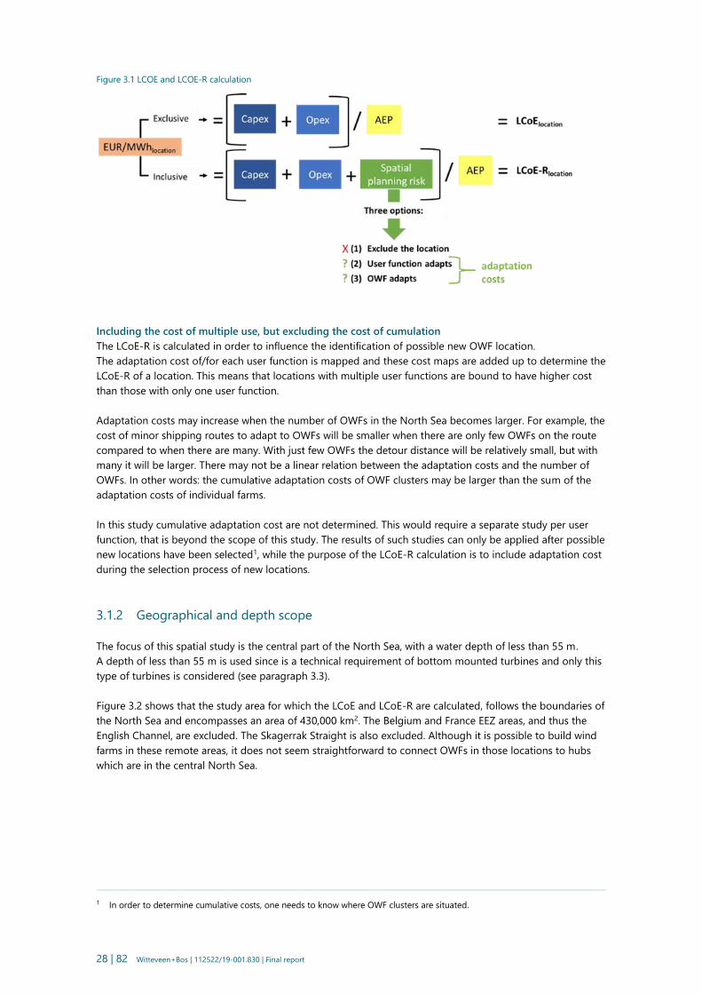
Figure 3.1 LCOE and LCOE-R calculation
Including the cost of multiple use, but excluding the cost of cumulation
The LCoE-R is calculated in order to influence the identification of possible new OWF location.
The adaptation cost of/for each user function is mapped and these cost maps are added up to determine the
LCoE-R of a location. This means that locations with multiple user functions are bound to have higher cost
than those with only one user function.
Adaptation costs may increase when the number of OWFs in the North Sea becomes larger. For example, the
cost of minor shipping routes to adapt to OWFs will be smaller when there are only few OWFs on the route
compared to when there are many. With just few OWFs the detour distance will be relatively small, but with
many it will be larger. There may not be a linear relation between the adaptation costs and the number of
OWFs. In other words: the cumulative adaptation costs of OWF clusters may be larger than the sum of the
adaptation costs of individual farms.
In this study cumulative adaptation cost are not determined. This would require a separate study per user
function, that is beyond the scope of this study. The results of such studies can only be applied after possible
new locations have been selected1, while the purpose of the LCoE-R calculation is to include adaptation cost
during the selection process of new locations.
3.1.2 Geographical and depth scope
The focus of this spatial study is the central part of the North Sea, with a water depth of less than 55 m.
A depth of less than 55 m is used since is a technical requirement of bottom mounted turbines and only this
type of turbines is considered (see paragraph 3.3).
Figure 3.2 shows that the study area for which the LCoE and LCoE-R are calculated, follows the boundaries of
the North Sea and encompasses an area of 430,000 km2. The Belgium and France EEZ areas, and thus the
English Channel, are excluded. The Skagerrak Straight is also excluded. Although it is possible to build wind
farms in these remote areas, it does not seem straightforward to connect OWFs in those locations to hubs
which are in the central North Sea.
1 In order to determine cumulative costs, one needs to know where OWF clusters are situated.

29 | 82 Witteveen+Bos | 112522/19-001.830 | Final report
Figure 3.2 Geographical scope of the study
3.1.3 Roll-out scope
This study also aims to identify both attractive new OWF locations and attractive grid roll-out pathways for
after 2030. The main purpose of this study is to identify possible locations and not to determine the final
wind energy capacity of the North Sea. Therefore the designed roll-out pathways may differ in terms of:
- wind farm locations and their grid connection system;
- the total amount of GW that is realized.
3.1.4 Cost scope
For both individual locations and for roll-out pathways both the LCoE and LCoE-R are calculated. The scope
of these calculations is to include costs that are distinctive for both location choice and grid roll-out path.
Cost components, such as onshore grid reinforcement, energy storage and Power to Gas, are very uncertain
and similar for locations and grid roll-out and are therefore not included (in LCoE). As a first approximation
for minimising grid integration cost, deeper inland connections have been considered which connect
offshore transmission cables to locations where available connection capacity is expected based on fossil fuel
phase-out scenarios.
However, spatial planning costs that are too small to have an impact on location choice and/or grid roll-out,
are always included (in LCoE-R) for the sake of respecting other sea users interests. A spatial planning cost
that may be small in relation to the cost of energy production, may be large in relation to the economic
value of the relevant spatial user function. These spatial planning costs are specified in chapter 4.2.2.
It may be noted that some aspects are not taken into account within the LCoE analysis due to their data
needs and the expectation that these aspects have little or no impact on the comparison of locations across
the North Sea. For example, decommissioning costs, blade degradation and wind hysteresis have not been
included in the LCoE calculation. The impact on the LCoE was considered similar across OWFs areas across
the North Sea. In paragraph 4.1.4 these omissions are discussed in relation to the uncertainty margins of the
LCoEs calculated in this study.
30 | 82 Witteveen+Bos | 112522/19-001.830 | Final report
Spatial risk without process costs
It should be noted here that the spatial costs do not include the extra process costs that are likely to occur
whenever a wind farm meets another user function e.g. project delays or additional costs for permitting.
Even if there is no conflict, stakeholders will fend for their interests and there will be communication cost on
part of the wind farm developers and on part of the stakeholders i.e. user functions and on part of the
involved governments.
Though the process cost could be significant, their magnitude cannot easily be determined and included in
the spatial cost calculations. It would entail finding out how much extra procedure time is spent (e.g. on law
suits and negotiations) each time a wind farm has engage with another user function. This does not fit within
the scope and timeframe of this study. It is recognized that the spatial planning cost could be
underestimated due to excluding process cost. Since the cost of all user functions are underestimated, this
will not significantly influence the relative difference between user functions. It will however influence the
absolute magnitude of the spatial planning cost and thus particularly the LCoE-R of locations with multiple
users.
Another possible source of underestimation of spatial planning costs is that the cumulative cost of spatial
claims (i.e. of co-utilization) of the total OWF deployment is not part of the scope of this study.
3.2 Trends in of offshore wind energy production
In order to determine the future wind farm lay out and future grid connection for the year 2030 trends in
turbine size, wind farms size, power density and grid connection are investigated.
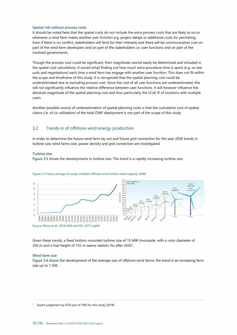
Turbine size
Figure 3.3 shows the developments in turbine size. The trend is a rapidly increasing turbine size.
Figure 3.3 Yearly average of newly-installed offshore wind turbine rated capacity (MW)
Source: Remy et al., 2018 (left) and IEA, 2013 (right)
Given these trends, a fixed bottom mounted turbine size of 15 MW (monopile, with a rotor diameter of
250 m and a hub height of 155 m seems realistic for after 20301.
Wind farm size
Figure 3.4 shows the development of the average size of offshore wind farms: the trend is an increasing farm
size up to 1 GW.
1 Expert judgement by ECN part of TNO for this study (2018).

31 | 82 Witteveen+Bos | 112522/19-001.830 | Final report
Figure 3.4 Average size of OWF projects (MW) commissioned per year
Source: Remy et al., 2018
Considering these developments, future OWFs are expected to have a capacity of 1 GW by the year 2030.
Farm power density
Current power densities vary among existing OWFs in the North Sea and range from approximately 4 to
14 MW/km2 (Bulder et al. 2018)1. A decrease in farm power density is expected because larger spacing
between turbines reduces the wake effects (i.e. turbines ‘stealing’ each other’s wind2) that occur inside wind
farms and in clusters of wind farms (Bulder et al., 2018).
Based on the expected optimal farm power density by ECN part of TNO for the year 2030, a reference power
density of 3.6 MW/km2 is used in this study.
Grid reinforcement
Large scale offshore wind energy production is likely to require onshore grid reinforcement due to increasing
demand-supply distances and increasing peak loads.
The distance between electricity demand centres and supply will probably grow. Power plants near energy
demand centres will likely be replaced by wind and solar farms that are located offshore and in rural areas. In
rural areas the local grid cannot handle the energy supply of wind and solar farms. As a consequence,
offshore transmission system operators need to construct new offshore grids to bring energy ashore. They
may also need to reinforce onshore connection points and the onshore power grid.
Peak loads may increase for two reasons:
- heating of buildings, mobility and industrial production will be electrified;
- base load power plants are replaced by intermittent renewable sources, which require more installed
capacity (MW) for the same amount of energy production (MWh).
Increasing peak loads will likely require electricity grid reinforcement, but both hydrogen conversion and
energy storage can lower the need for this reinforcement. By 2030 hydrogen could play a role in heating,
mobility and industry, possibly resulting in less electrification. When applied to wind and solar farms,
hydrogen conversion and energy storage could flatten renewable energy sources’ intermittent nature and
thereby reduce the need for grid reinforcement.
1 PBL’s report "The Future of the North Sea" (Matthijsen, J., E. Dammers and H. Elzenga, 2018) uses a power density of 6
MW/km2, whereas the Wind Europe's "Unleashing offshore wind potential" (Hundleby, G. and K. Freeman, 2017) uses a power
density of 5.4 MW/km2.
2 Wind farms are “blocked” by other wind farms and become dependent on a vertical flux of wind energy from higher layers.
32 | 82 Witteveen+Bos | 112522/19-001.830 | Final report
Given these developments it is expected that large scale offshore wind energy production will lead to extra
costs to reinforce the onshore grid. The required magnitude of these reinforcements is deeply unknown and
not easy to predict. It would require a special prediction study. Such a prediction study does not fit within
the scope and timespan of this study. Consequently, grid reinforcement costs are not included in the LCoE
calculations in this study.
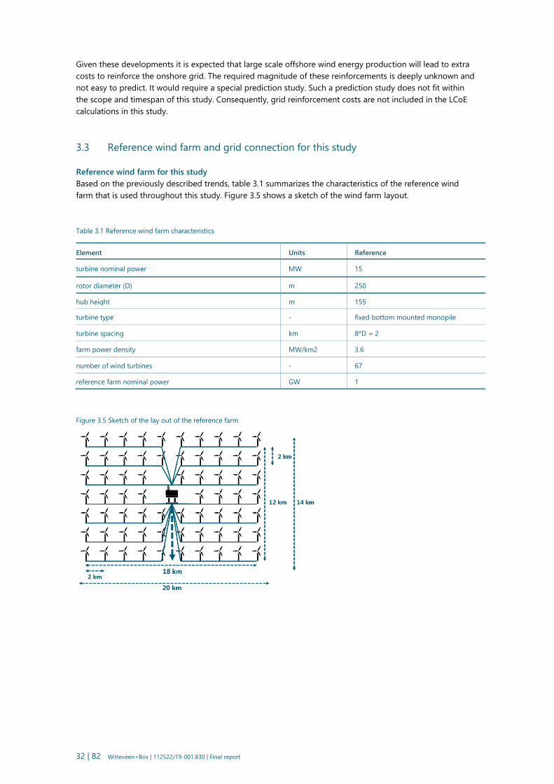
3.3 Reference wind farm and grid connection for this study
Reference wind farm for this study
Based on the previously described trends, table 3.1 summarizes the characteristics of the reference wind
farm that is used throughout this study. Figure 3.5 shows a sketch of the wind farm layout.
Table 3.1 Reference wind farm characteristics
Element Units Reference
turbine nominal power MW 15
rotor diameter (D) m 250
hub height m 155
turbine type - fixed bottom mounted monopile
turbine spacing km 8*D = 2
farm power density MW/km2 3.6
number of wind turbines - 67
reference farm nominal power GW 1
Figure 3.5 Sketch of the lay out of the reference farm

33 | 82 Witteveen+Bos | 112522/19-001.830 | Final report
Reference grid connection systems for this study
For the offshore grid connection, the following starting points are used throughout this study:
- transmission of power generated by the OWFs is through the use of electrical infrastructure only;
- three electrical GCSs are used: AC radial, DC radial and hub and spoke (H&S) are the three reference grid
connection systems considered in this study;
- only existing onshore grid connection points are used (see figure 3.6, left top)1;
- onshore grid reinforcements are not accounted in the reference grid connection.
Figure 2.2 in chapter 2.2 provides a sketch of the three reference grid connection systems that are used in
this study.
3.4 Used input data
In this study several data sources are used. These concern OWF-locations that have already been planned up
to the year 2030 by the North Sea countries’ governments, i.e. The baseline parks, maps with onshore
landing points, port, water depth, wind speed, waves and maps with the different space uses at the North
Sea such as fisheries and shipping. Table 3.2 provides an overview of the key data used and their sources.
Figure 3.6 shows the key maps that were used as starting points.
Table 3.2 Key input data
Input Source
baseline OWF Vree and Verkaik, (2017), NSWPH consortium, The Crown Estate UK
onshore landing points Vree and Verkaik, (2017)
ports ports.com
depth EMODnet-bathymetry.eu
windspeed at hub height (155 m) NOAA NCEP Climate Forecast System Reanalysis (CFSR)
windspeed at 10 m NOAA Wavewatch III
waves
cost information OWF
cost information GCS
cost information sandy hub islands
space use by other functions
NOAA Wavewatch III
ECN part of TNO cost modelling with simulations for operation and
maintenance, for substructure and for energy yield and wake losse
experience numbers provided by the NSWPH consortium2
Klomp et al., (2014)
Imares maps (Jongbloed et al., 2014)
Chapter 4 provides the key economic parameters used as starting points. For most spatial user functions
GIS maps generated by IMARES (Jongbloed et al., 2014) are used: this source is chosen because it is North
Sea covering and the maps- particularly the maps for nature and shipping- are tailor made for offshore wind
studies. Appendix I presents the space use maps that were used in this study. In this appendix it is also
described if and how the space use was updated for the year 2030 by investigating trends.
1 The onshore grid connection points were derived from a study by Vree and Verkaik (2017), which forecasted the future
available hosting capacity of these onshore grid connection points based on the expected phasing-out of fossil fuelled power
generation.
2 These cost estimates are based on internal cost estimates by TenneT and Energinet.

34 | 82 Witteveen+Bos | 112522/19-001.830 | Final report
Figure 3.6 Ports, landing points (left top), depth (right top), wind speed (left bottom), wave height (right bottom)
Source: LCoE-R mapping model developed in this study

35 | 82 Witteveen+Bos | 112522/19-001.830 | Final report
4
LCOE-R MAPPING MODEL
In this chapter new potential OWF locations are identified on the basis of North Sea covering LCoE and
LCoE-R maps. First, the key principles and calculation formulas of the LCoE and LCoE-R maps are explained.
Subsequently, the resulting LCoE and LCoE-R maps are presented and finally potential new locations are
identified by means of these maps.
4.1 LCoE mapping
In this study, a grid based North Sea covering LCoE mapping model was built, inspired by Gerrits (2017), as a
tool for identifying new OWF locations for the period after 2030. This mapping model consists of basic maps,
with a resolution of 1/48 degree in longitude and latitude, such as water depth, wave height and wind speed,
which determine costs and yields of an OWF. The model contains calculation formulas for all wind farm cost
components, for energy yields and for all grid connection cost components of the three considered GCSs
(AC radial, DC radial and H&S).
4.1.1 LCoE formula
The levelized cost of energy (LCoE) is calculated on the basis of a reference OWF of 1 GW. This means that
for every grid cell in the North Sea, the total cost to build and operate the reference wind farm there are
estimated. In order to estimate these total costs, cost formulas that predict the cost on the basis of
metocean conditions (such as water depth and wind speed), were developed for all OWF components (such
as turbines and intra array cables) and for all GCS components (such as cables to land and transformer
substations).
The LCoE calculation is based on the formula shown below. This formula considers:
- the annuity factor a of 20 years;
- the capital expenditure CapEx, for which there is a cost formula for investment for every component;
- the yearly operational expenditure OpEx which were either a fixed yearly value or a percentage of CapEx;
- the Annual Energy Production AEP, which is effected by:
· availability of the OWF and the GCS;
· energy losses per OWF and GCS component.
Annuity (a)
The annuity (a) is used to determine a yearly value for CapEx. It depends on the discount rate and the
depreciation period. A real discount rate of 2.9 % and a depreciation period of 30 years are used in this
study, resulting in an annuity of approximately 20 years. Table 4.1 shows these assumptions.
36 | 82 Witteveen+Bos | 112522/19-001.830 | Final report
Table 4.1 Economic assumptions*
Component Assumption
nominal discount rate (R) 4.4 %
inflation rate (i) 1.5 %
real discount rate (r = (1+R)
(1+i)− 1) 2.9 %
depreciation period 30 years
annuity (a =1−(1+𝑟)−𝑛
𝑟 ) 20 years
* Based on international study results commissioned by the NSWPH consortium
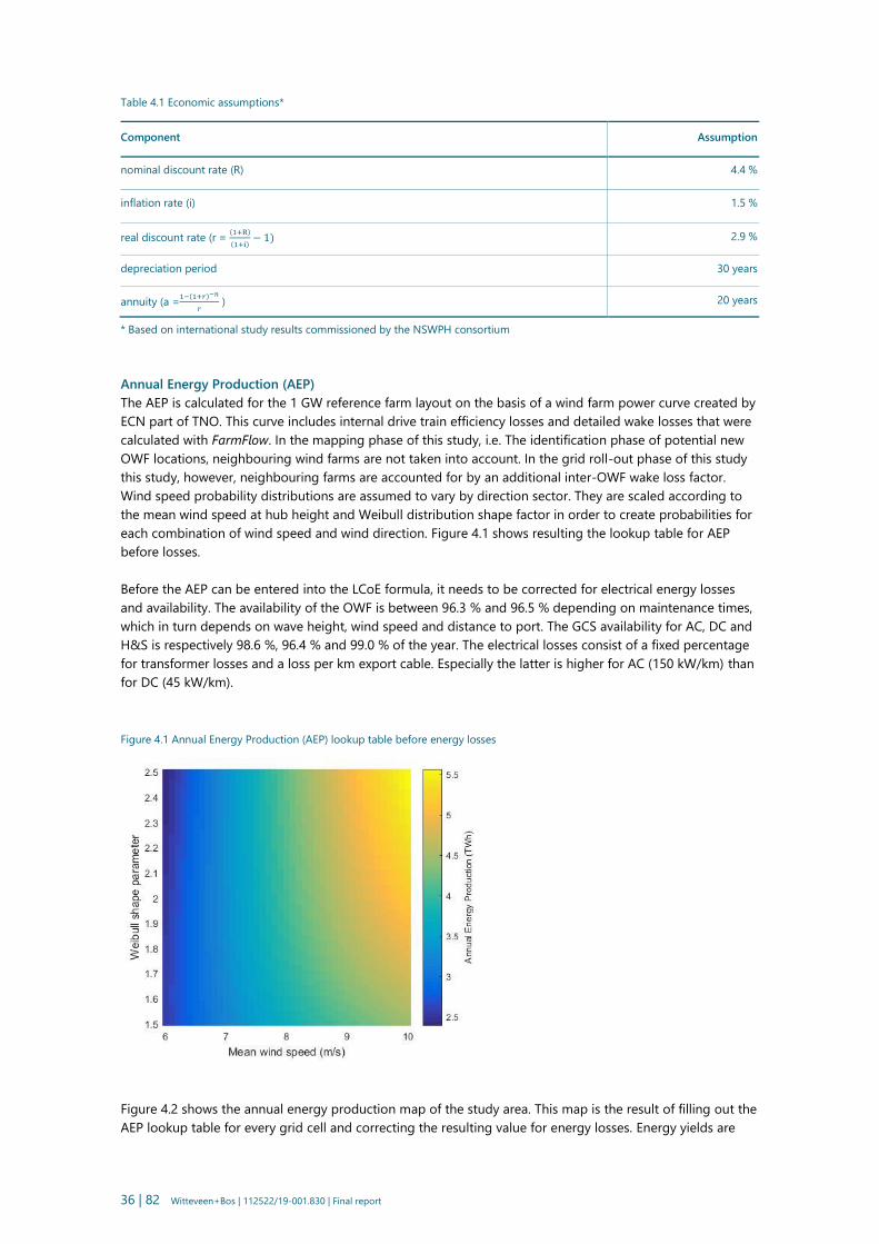
Annual Energy Production (AEP)
The AEP is calculated for the 1 GW reference farm layout on the basis of a wind farm power curve created by
ECN part of TNO. This curve includes internal drive train efficiency losses and detailed wake losses that were
calculated with FarmFlow. In the mapping phase of this study, i.e. The identification phase of potential new
OWF locations, neighbouring wind farms are not taken into account. In the grid roll-out phase of this study
this study, however, neighbouring farms are accounted for by an additional inter-OWF wake loss factor.
Wind speed probability distributions are assumed to vary by direction sector. They are scaled according to
the mean wind speed at hub height and Weibull distribution shape factor in order to create probabilities for
each combination of wind speed and wind direction. Figure 4.1 shows resulting the lookup table for AEP
before losses.
Before the AEP can be entered into the LCoE formula, it needs to be corrected for electrical energy losses
and availability. The availability of the OWF is between 96.3 % and 96.5 % depending on maintenance times,
which in turn depends on wave height, wind speed and distance to port. The GCS availability for AC, DC and
H&S is respectively 98.6 %, 96.4 % and 99.0 % of the year. The electrical losses consist of a fixed percentage
for transformer losses and a loss per km export cable. Especially the latter is higher for AC (150 kW/km) than
for DC (45 kW/km).
Figure 4.1 Annual Energy Production (AEP) lookup table before energy losses
Figure 4.2 shows the annual energy production map of the study area. This map is the result of filling out the
AEP lookup table for every grid cell and correcting the resulting value for energy losses. Energy yields are

37 | 82 Witteveen+Bos | 112522/19-001.830 | Final report
relatively high in north eastern part of the sea. The colour legend of figure 4.2 reveals that the annual energy
production ranges from 2.7 to 5.4 TWh per year. This corresponds with a capacity factor of 30 to 62 %.
Figure 4.2 Annual energy production map of the North Sea
Source: LCoE-R mapping model developed in this study
4.1.2 OWF cost formulas
ECN part of TNO has developed formulas for this study to estimate the capital and operational expenditures
of the different OWF components. The CapEx components are wind turbine, substructure, intra array cables
project development and installation. The OpEx consists of operation and maintenance. The cost formulas of
these components were entered into the LCoE formula. The results of this exercise can be summarized in the
form of lookup tables. Figure 4.3 shows these look up tables for radial AC or DC and figure 4.4 for H&S1.
Figure 4.3 LCoE OWF look up table for radial AC or DC
1 For both lookup tables a reference AEP of 5 TWh was used. In the mapping tool the location specific AEP is used.
38 | 82 Witteveen+Bos | 112522/19-001.830 | Final report
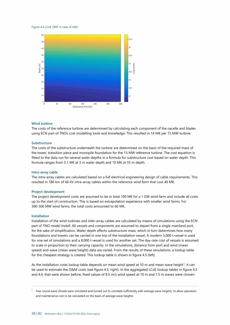
Figure 4.4 LCoE OWF in case of H&S
Wind turbine
The costs of the reference turbine are determined by calculating each component of the nacelle and blades
using ECN part of TNOs cost modelling tools and knowledge. This resulted in 14 M€ per 15 MW turbine.
Substructure
The costs of the substructure underneath the turbine are determined on the basis of the required mass of
the tower, transition piece and monopile foundation for the 15 MW reference turbine. The cost equation is
fitted to the data run for several water depths in a formula for substructure cost based on water depth. This
formula ranges from 5.1 M€ at 5 m water depth and 10 M€ at 55 m depth.
Intra-array cable
The intra-array cables are calculated based on a full electrical engineering design of cable requirements. This
resulted in 180 km of 66 kV intra-array cables within the reference wind farm that cost 40 M€.
Project development
The project development costs are assumed to be in total 100 M€ for a 1 GW wind farm and include all costs
up to the start of construction. This is based on extrapolation experience with smaller wind farms. For
300-500 MW wind farms, the total costs amounted to 60 M€.
Installation
Installation of the wind turbines and inter-array cables are calculated by means of simulations using the ECN
part of TNO model Install. All vessels and components are assumed to depart from a single mainland port,
for the sake of simplification. Water depth affects substructure mass, which in turn determines how many
foundations and towers can be carried in one trip of the installation vessel. A modern 5,000 t vessel is used
for one set of simulations and a 8,000 t vessel is used for another set. The day-rate cost of vessels is assumed
to scale in proportion to their carrying capacity. In the simulations, distance from port and wind (mean
speed) and wave (mean wave height) data are varied. From the results of these simulations, a lookup table
for the cheapest strategy is created. This lookup table is shown in figure 4.5 (left).
As the installation costs lookup table depends on mean wind speed at 10 m and mean wave height1, it can
be used to estimate the O&M costs (see figure 4.5, right). In the aggregated LCoE lookup tables in figure 4.3
and 4.4, that were shown before, fixed values of 8.5 m/s wind speed at 10 m and 1.5 m waves were chosen.
1 Year round wave climats were simulated and turned out to correlate sufficiently with average wave heights, to allow operation
and maintenance cost to be calculated on the basis of average wave heights.

39 | 82 Witteveen+Bos | 112522/19-001.830 | Final report
Figure 4.5 OWF installation costs (left) and OWF O&M costs (right)
Operation & Maintenance (O&M)
The main difference for the OpEx between the three grid connection systems is that for AC and DC,
maintenance takes place from the nearest mainland port, while for H&S it takes place from the port on the
hub. Several maintenance strategies were simulated using ECN part of TNO model O&M Calculator including
2 and 3 crew transfer vessels with helicopter, 1 service operation vessel plus helicopter and 2 service
operation vessels. For each strategy, simulations are run to cover variations in distance from port, wind and
wave data. From the results of these simulations, a lookup table for the cheapest strategy (while maintaining
sufficiently high availability) is created. This lookup table is shown in figure 4.5 (right).
From the lookup table it can be concluded that both distance to port and wave height only have a limited
influence on O&M costs. There appears to be only 3.5 % O&M costs difference between nearshore areas
with low waves (45 M€) and far offshore areas with high average waves (47 M€). Therefore a hub with O&M
facilities appears to offer only a modest cost advantage to AC and DC radial. A separate study is being
conducted to further analyse this aspect.
4.1.3 GCS cost formulas
Cost for each of the three considered grid connection systems (GCS) and their individual components have
been determined by the NSWPH consortium. The costs components that ware taken into account are
offshore transformer substation costs which scale with water depth, export cables to shore costs which scale
with cable length and onshore transformer substations costs which are fixed costs. The OpEx for the GCS is
defined per component and either assumed as a fixed amount or as a percentage of the CapEx of that
component. Entering the costs of the various components into the LCoE formula results in LCoE GCS lookup
tables. Figure 4.6 and 4.7 show these lookup tables for radial AC and DC.
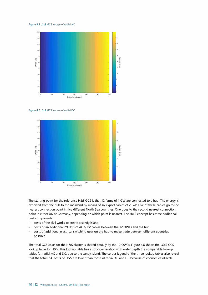
40 | 82 Witteveen+Bos | 112522/19-001.830 | Final report
Figure 4.6 LCoE GCS in case of radial AC
Figure 4.7 LCoE GCS in case of radial DC
The starting point for the reference H&S GCS is that 12 farms of 1 GW are connected to a hub. The energy is
exported from the hub to the mainland by means of six export cables of 2 GW. Five of these cables go to the
nearest connection point in five different North Sea countries. One goes to the second nearest connection
point in either UK or Germany, depending on which point is nearest. The H&S concept has three additional
cost components:
- costs of the civil works to create a sandy island;
- costs of an additional 290 km of AC 66kV cables between the 12 OWFs and the hub;
- costs of additional electrical switching gear on the hub to make trade between different countries
possible.
The total GCS costs for the H&S cluster is shared equally by the 12 OWFs. Figure 4.8 shows the LCoE GCS
lookup table for H&S. This lookup table has a stronger relation with water depth the comparable lookup
tables for radial AC and DC, due to the sandy island. The colour legend of the three lookup tables also reveal
that the total CSC costs of H&S are lower than those of radial AC and DC because of economies of scale.
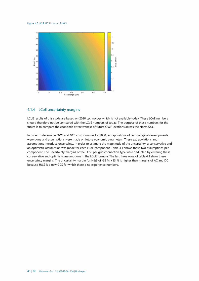
41 | 82 Witteveen+Bos | 112522/19-001.830 | Final report
Figure 4.8 LCoE GCS in case of H&S
4.1.4 LCoE uncertainty margins
LCoE results of this study are based on 2030 technology which is not available today. These LCoE numbers
should therefore not be compared with the LCoE numbers of today. The purpose of these numbers for the
future is to compare the economic attractiveness of future OWF locations across the North Sea.
In order to determine OWF and GCS cost formulas for 2030, extrapolations of technological developments
were done and assumptions were made on future economic parameters. These extrapolations and
assumptions introduce uncertainty. In order to estimate the magnitude of the uncertainty, a conservative and
an optimistic assumption was made for each LCoE component. Table 4.1 shows these two assumptions per
component. The uncertainty margins of the LCoE per grid connection type were deducted by entering these
conservative and optimistic assumptions in the LCoE formula. The last three rows of table 4.1 show these
uncertainty margins. The uncertainty margin for H&S of -32 % +53 % is higher than margins of AC and DC
because H&S is a new GCS for which there a no experience numbers.

42 | 82 Witteveen+Bos | 112522/19-001.830 | Final report
Table 4.1 Uncertainty margins on LCoE input components and results
Component Assumed
uncertainty
margin
Explanation
CapEx OWF (M€) -7 % +14 % There are no real cost data available for a 15 MW wind turbine. It is, however, possible
to calculate the material volumes needed to construct a 15 MW wind turbine with a
rotor diameter of 250 m with reasonably accuracy. Furthermore, it is assumed that the
future trend in component cost is comparable with past developments. This implies that
innovations achieved in the past will continue in the future, which induces an
uncertainty margin of +/-10 % for CapEx OWF.
Decommissioning cost were not included in the LCoE of this study. ECN part of TNO has
estimated the costs of decommissioning comparable (170 M€) or lower (120 M€) than
the installation costs. The present values of these costs are respectively 70 M€ and 50
M€. Including these costs in the CapEx uncertainty shifts the margin of +/-10 % to -7 %
and +14 %.
OpEx OWF
(M€/year)
+/-25 % The uncertainty is explained by the fact that there is substantially less data available to
extrapolate the O&M costs from the present size to the 15 MW wind turbine.
CapEx and OpEx
GCS AC (M€)
+/-10 % The specified AC radial concept is relatively close to that of several (to be) realized
offshore wind projects, rendering the uncertainty range small.
CapEx and OpEx
GCS DC (M€)
and (M€/year)
-10 % +15 % The specified DC radial concept is relatively close to that of (to be) realized projects, as
such the uncertainty range is small.
CapEx and OpEx
GCS H&S (M€)
and (M€/year)
-20 % +30 % The uncertainty range is explained by the fact that several factors which impact the cost
assumptions, are still to be validated as the H&S concepts has not yet been applied. On
the one hand potential risks need to be accounted for, substantiating the upper range,
while an optimization of the island design substantiates the lower range of the CapEx.
AEP (TWh/year) -4.9 % +4.3 %. Uncertainty in wind resources and consequently the yield of a wind farm is set at 4 % .
In general the annual average wind speed uncertainty is assumed to be approximately 4
%, which is the 20 year uncertainty. The uncertainty in the wake analysis is actually quite
small and it is assumed that this can be included by increasing the uncertainty in the
average wind speed by 1 % to 5 %. This uncertainty does not include the variation of
wind speed from year to year which can be much more than 4 %. The energy yield
uncertainty based on a 5 % uncertainty in the average wind speed is determined to be -
4.9 % and +4.3 %.
Annuity (years) -21 % +26 % Uncertainty of the annuity is determined by the assumptions on the nominal discount
rate, inflation rate and the depreciation period (see table 4.1). A nominal discount rate
between 4.0 % and 5.0 % and an inflation rate between 1.0 % and 2.0 % result in a real
discount rate between 2.0 % and 4.0 %. The depreciation period or reasonable OWF
lifetime is between 25 and 35 years. This results in an annuity between 16 and 25 years.
LCoE for AC
(€/MWh)
-29 % +41 % This is the resulting uncertainty margin of an LCoE calculation with the above
mentioned uncertainty assumptions per component for AC radial.
LCoE for DC
(€/MWh)
-29 % +46 % This is the resulting uncertainty margin of an LCoE calculation with the above
mentioned uncertainty assumptions per component for DC radial.
LCoE for H&S
(€/MWh)
-32 % +53 % This is the resulting uncertainty margin of an LCoE calculation with the above
mentioned uncertainty assumptions per component for H&S.
From table 4.1 one can conclude that the LCoEs calculated in this study have an uncertainty range of
approximately -30 % to +50 %.
It may be noted that decommissioning costs, blade degradation and wind hysteresis were not included in
the LCoE calculations in this study. To account for the omission of decommission costs, they were included in
the uncertainty margin of CapEx OWF. Including these decommissioning costs in the CapEx uncertainty
increased the margin from of +/-10 % to -7 % and +14 %.

43 | 82 Witteveen+Bos | 112522/19-001.830 | Final report
According to ECN part of TNO, blade degradation cost are marginal. Monitoring results in wind farms show
that energy yields are mainly determined by wind speed and are not diminishing as the OWF ages and
turbine blades degrade. Yield losses due to high wind speed hysteresis is probably also negligible, as the
shut down time is limited. Modern turbines no longer shut down at wind speeds higher than 25 m/s, but
continue producing at a lower level.
4.1.5 LCoE maps
Figure 4.5 shows the LCoE maps that were created by means of the cost formulas described in the previous
paragraphs. There is a separate LCoE map for the three grid connection systems AC radial, DC radial and
H&S.
The AC map shows that locations with a relatively low LCoE in case of an AC GCS can be found close to
shore. According to the DC map locations with a relatively low LCoE in case of a DC GCS are situated slightly
further from shore. The H&S map reveals that locations with relatively low LCoE, when applying H&S GCS,
are found everywhere except for the most central part of the study area and nearshore.
Figure 4.5 LCoE maps per grid connection system (top to bottom: AC radial, DC radial and hub and spoke)

44 | 82 Witteveen+Bos | 112522/19-001.830 | Final report
Source: LCoE mapping model developed in this study

45 | 82 Witteveen+Bos | 112522/19-001.830 | Final report
4.2 LCoE-R mapping
In this study not only LCoE maps, but also LCoE-R maps are developed. LCoE-R maps include the cost of
encountering other user functions. For each spatial user function a map is created that reflects the monetary
value of the risk of encountering that function when developing an OWF. The spatial risk maps are made by
multiplying reference spatial user maps (as presented in appendix I) with a risk formula. Risk formulas are
developed on the basis of a previous societal cost benefit study (Hoefsloot et al., 2018) in which the risk of
each user function was specified in concertation with the relevant stakeholders.
4.2.1 Spatial risk principles
In principle, there are three ways to monetarize spatial risk: exclusion of zones,
function adaptation or OWF adaption. This results from the fact that every time
an OWF encounters a spatial user function, there are three ways to deal with a
potential spatial conflict, that each lead to different costs.
1. Exclusion of zones: zones with other user functions are excluded from the search area for wind energy.
This is the most explored option so far in search studies for new OWF locations. The calculation of spatial
costs now boils down to the cost difference per produced MWh between locations claimed by other sea
users and locations not yet claimed by other sea users.
2. The user function adapts to the OWF: when an OWF encounters another sea user, this user function
adapts itself to the energy production. This could mean that the function moves to another location. Then
there will be movement cost (e.g. military exercises are moved to another area). It could also mean that the
function ceases to exist and then its net benefits will be lost (e.g. the fish will not be caught).
Another possibility is that the user function stays inside the wind farm, i.e. there is co-use. In such cases the
user function may suffer efficiency losses1 (e.g. fishing is carried out less efficiently in wind farms). In case the
user functions adapts, the spatial costs are the damage cost of the effected user function.
3. The OWF adapts to the user function: when another sea user is met, OWFs can also adapt themselves in
such a way that damage to the other user is prevented or mitigated. This could entail an adjustment of the
wind farm layout (e.g. moving a couple of turbines to respect the helicopter zone of an oil & gas platform).
This leads to extra farm development cost (e.g. extra cable length to connect turbines). It could also involve
taking extra precautionary measures (e.g. shutting turbines down for the sake of bird migration) or
restoration measures (e.g. applying Building with Nature solutions to stimulate nature restoration). In case
the OWF adapts, the spatial cost are equal to costs of actions taken by the wind farm developer.
In the LCoE-R calculation, only the last two options are considered, as the approach of this spatial study is to
avoid excluding potential OWF locations.
Ideally cost of both user function adaptation and OWF adaptation would be determined for all relevant
spatial user function. This would reveal which of these two options is the cheapest and then the cheapest
option could be used to calculate the LCoE-R. In practice, this does not seem relevant for every user function.
Table 4.6 gives an overview of the selected option(s) and underlying motives for the spatial cost calculation
of each user function.
1 Either due to extra production cost (e.g. extra transport cost for fishing vessels) or yield reductions (e.g. less fish caught).

46 | 82 Witteveen+Bos | 112522/19-001.830 | Final report
Table 4.6 Spatial user functions and their basis for cost calculation
Spatial
user
function
Selected risk
principle
Motivation Description of the spatial cost
Military
zones
Function adapts It does not seem possible to make
OWF compatible with military
exercises. Therefore the option that
the user function adapts is selected.
If a large part of a military zone (i.e. >20 %) is covered by
wind turbines, the zone becomes unusable for military
exercise, so there will be cost of practicing elsewhere:
relocation cost.
If a small part of a military zone (<20 %) is used for wind
energy, it is possible to mitigate this change by adapting
the procedures i.e. adapting the organization and
planning of military exercises: reorganization costs.
Nature:
sea
mammals
OWF adapts Trying to get mammals to adapt to
OWF is not relevant/possible; the
key of nature policies is not to
disturb mammals
The spatial cost are equal to cost of preventing mammal
disturbance: the extra costs of gentle piling (compared
to regular piling).
Nature:
birds
OWF adapts Attempting to get birds to adapt to
OWF is not relevant nor feasible, as
it is difficult to create sufficient new
bird habitats and to actively
influence bird flying routes.
The spatial cost are equal to the cost of preventing bird
population losses by turbine shut downs: the cost of
energy yield reduction. Damage to migratory birds due
to collisions can be prevented by real time radar
monitoring of birds: at >500 birds per km2/hour at rotor
height, turbines are shut down. Experience near shore:
30 hours per year shut down. Damage to sea birds, due
to habitat loss, can possibly be prevented by larger
turbines & larger inter turbine space. Maybe, increasing
food availability (fish) and/or turbine shut downs during
foraging periods can also help; deterring birds should be
avoided as it evokes habitat loss instead of limiting it.
Nature:
bats
OWF adapts Attempting to get bats to adapt to
OWF is not relevant/possible as it is
difficult to actively influence their
flying routes. Wind turbines & oil &
gas platforms seem to attract bat to
forage on insects.
The spatial cost are the cost of turbine shut down i.e.
energy production losses. Bats mainly migrate along the
shores of the North Sea. They seem to only fly across the
sea from Norway to UK. If an OWF interacts with a bat
flying route, turbines need to be shut down 10 hours per
day, during 45 days in September and August at wind
speeds of <5 m/s. They only fly at night and at low wind
speeds.
Nature:
habitats
OWF adapts Adapting habitats to OWF, seems
difficult as this would require large
scale nature development at sea. It
would also not be in line with
European nature protection policies,
which appointed certain areas to
safeguard them from being harmed
by economic activities.
The spatial cost of building OWF in protected nature
areas can be estimated in terms of the cost of actively
enhancing nature restoration by applying Building with
Nature solutions. Marine ecosystems can be enhanced
by stimulating reef builders such as flat oysters. This can
be realized with nature friendly scour protections or
other Building with Nature solutions.
Shipping
routes
For minor routes:
function adapts
Major routes: the
OWF adapts
For shipping routes with low
intensity it makes sense that ships
sail around wind farms, while for
routes with high intensity it makes
sense to create a shipping corridor
through the wind farm.
For minor routes (< 1 ship/day): wind farm layout
without a corridor; the shipping route is adapted,
leading to detour costs.
For major routes (> 1ship/day): wind farm layout with a
corridor, leading to extra cable cost to connect turbines
on both sides of the corridor.
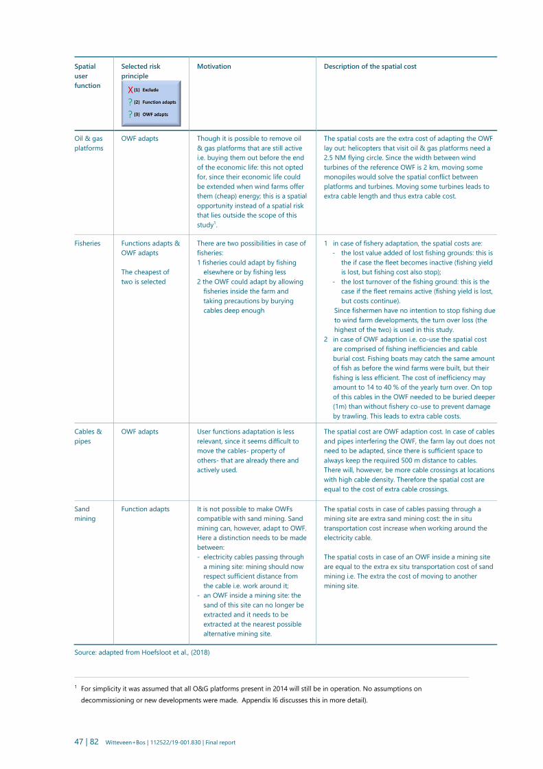
47 | 82 Witteveen+Bos | 112522/19-001.830 | Final report
Spatial
user
function
Selected risk
principle
Motivation Description of the spatial cost
Oil & gas
platforms
OWF adapts Though it is possible to remove oil
& gas platforms that are still active
i.e. buying them out before the end
of the economic life: this not opted
for, since their economic life could
be extended when wind farms offer
them (cheap) energy; this is a spatial
opportunity instead of a spatial risk
that lies outside the scope of this
study1.
The spatial costs are the extra cost of adapting the OWF
lay out: helicopters that visit oil & gas platforms need a
2.5 NM flying circle. Since the width between wind
turbines of the reference OWF is 2 km, moving some
monopiles would solve the spatial conflict between
platforms and turbines. Moving some turbines leads to
extra cable length and thus extra cable cost.
Fisheries Functions adapts &
OWF adapts
The cheapest of
two is selected
There are two possibilities in case of
fisheries:
1 fisheries could adapt by fishing
elsewhere or by fishing less
2 the OWF could adapt by allowing
fisheries inside the farm and
taking precautions by burying
cables deep enough
1 in case of fishery adaptation, the spatial costs are:
- the lost value added of lost fishing grounds: this is
the if case the fleet becomes inactive (fishing yield
is lost, but fishing cost also stop);
- the lost turnover of the fishing ground: this is the
case if the fleet remains active (fishing yield is lost,
but costs continue).
Since fishermen have no intention to stop fishing due
to wind farm developments, the turn over loss (the
highest of the two) is used in this study.
2 in case of OWF adaption i.e. co-use the spatial cost
are comprised of fishing inefficiencies and cable
burial cost. Fishing boats may catch the same amount
of fish as before the wind farms were built, but their
fishing is less efficient. The cost of inefficiency may
amount to 14 to 40 % of the yearly turn over. On top
of this cables in the OWF needed to be buried deeper
(1m) than without fishery co-use to prevent damage
by trawling. This leads to extra cable costs.
Cables &
pipes
OWF adapts User functions adaptation is less
relevant, since it seems difficult to
move the cables- property of
others- that are already there and
actively used.
The spatial cost are OWF adaption cost. In case of cables
and pipes interfering the OWF, the farm lay out does not
need to be adapted, since there is sufficient space to
always keep the required 500 m distance to cables.
There will, however, be more cable crossings at locations
with high cable density. Therefore the spatial cost are
equal to the cost of extra cable crossings.
Sand
mining
Function adapts It is not possible to make OWFs
compatible with sand mining. Sand
mining can, however, adapt to OWF.
Here a distinction needs to be made
between:
- electricity cables passing through
a mining site: mining should now
respect sufficient distance from
the cable i.e. work around it;
- an OWF inside a mining site: the
sand of this site can no longer be
extracted and it needs to be
extracted at the nearest possible
alternative mining site.
The spatial costs in case of cables passing through a
mining site are extra sand mining cost: the in situ
transportation cost increase when working around the
electricity cable.
The spatial costs in case of an OWF inside a mining site
are equal to the extra ex situ transportation cost of sand
mining i.e. The extra the cost of moving to another
mining site.
Source: adapted from Hoefsloot et al., (2018)
1 For simplicity it was assumed that all O&G platforms present in 2014 will still be in operation. No assumptions on
decommissioning or new developments were made. Appendix I6 discusses this in more detail).
48 | 82 Witteveen+Bos | 112522/19-001.830 | Final report
Table 4.6 shows that the spatial cost of encountering military zones, minor shipping routes and sand mining
are based on the principle that user functions adapts. Mostly the reason for choosing this principle is the
impossibility of difficulty to make OWFs compatible with the user function, while the user function can adapt
to the OWF.
The spatial costs of encountering nature (mammals, birds, bats, protected areas), major shipping routes, oil
and gas platforms, cables and pipes are based on the principle that the OWF adapts. Mostly the reason for
this choice is that it is relatively easy to adapt the wind farm lay out, while it is difficult or impossible for the
user function to adapt to OWFs.
Only for fisheries the spatial cost are determined both in terms of function adaptation and in terms of OWF
adaptation. Based on the calculation results the principle that generates the lowest cost could be selected.
As explained in chapter 3.1.4, process costs are not included in spatial planning costs.
4.2.2 LCoE-R calculations
In the previous paragraph the spatial risks of encountering other sea users were specified in terms of spatial
cost. In table 4.7 the spatial cost calculation formulas are presented. Since the calculations of spatial cost are
done on the basis of GIS maps of the spatial user function (see Appendix I), this table also shows the units of
the legend of the these maps. Since the spatial cost are included in the LCoE-R maps, it is also indicated
whether the cost are added to the capital expenditure or to the operational expenditure.
Military zones
The spatial costs of military zones are different for small zones and large zones. Based on earlier stakeholder
interviews (Hoefsloot et al., 2014 and 2010), it is assumed that in case of small zones, a reference wind farm
may render the zone too small for future practice and the organizations using the zone need to relocate
their exercises. In case of large zones a reference park may leave the zone useable, but military exercises
need to be reorganized. In previous societal cost studies (Hoefsloot et al., 2014 and 2018) these cost were
estimated in concertation with the Dutch ministry of defence. This resulted in expected relocation cost of
0.75 M€/year and expected reorganization cost of 2 M€ once (Hoefsloot et al., 2014 and 2018). The cost
formula divides these cost over the total km2 of a military zone.
Nature: sea mammals
The spatial cost in relation to mammals is the extra cost of gentle piling. These are already included in the
LCoE calculation (in the CapEx component i.e. The installation costs for the turbines) as gentle piling is the
standard building method. Calculating them again as a spatial cost would introduce a double counting and
is therefore refrained from.
Nature: birds
The spatial cost of birds pertains to lost energy yields due to shutting down turbines when large numbers of
birds are detected at rotor height. Presently, license prescriptions for OWFs state that at more than 500 birds
per hour at rotor height turbines need to shut down in order to prevent collision victims. Experience so far is
that this leads to approximately 30 shut down hours per year for OWFs near the coast (Kamp, 2016).
Figure 4.6 shows radar monitoring data on birds’ fluxes at rotor height in the Southern part of the North Sea
in the years 2007 to 2010. The peaks in early spring, which show fluxes of more than 500 birds per hour, are
most likely migratory birds flying from the Netherlands to the UK. Peaks in autumn, which also have more
than 500 birds per hour, probably reflect birds migrating from Sweden to the UK and to European mainland.

49 | 82 Witteveen+Bos | 112522/19-001.830 | Final report
Figure 4.6 Occurrence of birds in fluxes per hour at a rotor height
Source: Krijgsveld et al., (2015)
Figure 4.6 also shows that there are lower peaks as well: approximately seven peaks per year of more than
200 birds per hour. These findings suggest that in order not to cumulatively surpass the potential biological
removal limits of bird populations, turbine shut down hours may increase when the amount of deployed
megawatts increases in the North Sea. As a result the spatial costs of building OWFs in migratory routes and
probably also in sea bird sensitive areas, will also increase.
The issue with sea birds is that they are permanently present and they suffer from both habitat loss and
collision. Damage to sea birds can possibly be prevented by larger (and thus fewer) turbines and larger
inter-turbine space, though there are species for which this does not work. When these options become
exhausted, maybe increasing food availability through Building with Nature solutions and/or turbine shut
down during foraging periods may also help. This is highly uncertain. The spatial cost of sea birds is
therefore also highly uncertain.
In order to account for the fact that the cost of migratory birds may increase and the costs of sea birds
cannot be properly accounted for due to the lack of knowledge on effective mitigation measures, a
sensitivity analysis was carried out in which the known cost i.e. The shut down costs, were increased. In this
analyses the number of curtailment hours was increased by 500 hours (i.e. 7 seven peaks of 70 hours) for the
most sensitive areas and by 100 hours for the least sensitive areas of the WSI-map. The spatial cost resulting
from this analysis is included in figure 4.10 (top row, right side). In the LCoE-R calculation the lower
(presently relevant) 30 hour per year is used.
Nature: bats
The spatial costs concerning bats are lost energy yields of temporary turbine shut down. Though the
numbers to calculate these cost are available, no bat flying routes are found in the relevant parts of the study
area and therefore these cost are not calculated.
Nature: habitats
The spatial costs in relation to protected nature areas are determined on the basis of taking extra measures
to stimulate nature restoration inside the OWFs. The cost formula is based on the Building with Nature
solution ‘scour protection’ that stimulates reef builders i.e. flat oysters. These costs are estimated to
approximately 130 k€ per monopile (Lengkeek et al., 2017).
It may be noted that there are also other Building with Nature solutions, such as sea bed matrasses and bio-
huts for cod. The costs of these measures are not known yet. Pilot projects are needed to determine these
costs.

50 | 82 Witteveen+Bos | 112522/19-001.830 | Final report
Shipping routes
The spatial costs of minor shipping routes are calculated as average detour cost of ships that need to sail
around the OWF. The calculation formula for the detour cost is based on an average extra sailing distance of
6.6 km (see figure 4.6), a growth factor of 1.3 reflecting a high economic development scenario (Romijn et al,
2016) and transportation cost of 38 €/km (www.rwseconomie, cost barometer deep sea, 2016)1.
The spatial costs of major shipping routes are calculated by determining the cost of creating a corridor with
a width of 6.5 km (see figure 4.7). Such a corridor requires 7 to 102 extra cables of 6.5 km at a cost of
220 k€/km (ECN part of TNO estimate for this study)3.
For both major and minor routes, a fixed extra safety cost (for radar and surveillance) of approximately 10-
12 k€/km2 is added (based on Hoefsloot et al., 2018). Furthermore, it may be noted that for minor shipping
routes it is possible to also include the societal cost of the extra environmental pollution (i.e. emissions of
CO2, NOx and PM10) for each extra detour kilometre: the environmental cost double the transport cost per
km (Hoefsloot et al., 2018).
Figure 4.7 Calculating the spatial cost of shipping routes: minor (left), major (right)
Oil and gas platforms
The spatial cost of oil and gas platforms are the costs of adapting the lay out of the wind farm in such a way
the helicopters can safely land on the platforms. Since helicopters require a flying circle of 2.5 NM (Hoefsloot
et al., 2018), approximately sixteen turbines need to be moved 2 to 6 km, whenever a platform is
encountered (see figure 4.8). Moving turbines requires cable length and thus extra cable costs. The average
cost for inter array cable is estimated at 220 k€/km (ECN part of TNO estimate for this study). Dividing the
extra cable cost by the area of the flying circle results in a cost of approximately 330 k€/km2. When applying
this cost number to the reference map with oil and gas platforms, overlap between helicopter zones is
removed, in order not to overestimate spatial costs4.
1 Cost per km2 are derived by the dividing the cost by the area the reference windfarm.
2 Depending on whether the corridor is vertically (7 turbines) or horizontally (10 turbines) passing through the windfarm.
3 Cost per km2 are derived by the dividing the cost by the area of the corridor.
4 After drawing OWFs in the GIS mapping tool (see chapter 4), it was discovered that there are attractive farm location that have
so much overlap between helicopter zones, that one can actually not adapt the wind farm, so the oil & gas function needs to
adapt. This switch from ‘OWF adapts’ to ‘function adapts’ requires a different cost estimate: a cost formula that reflects the
extra cost of using boats instead of helicopters to visit the wind farms. This function is not developed in this study.
Consequently, the present spatial planning cost of oil & gas platforms may be underestimated for locations with many
overlapping helicopter zones.

51 | 82 Witteveen+Bos | 112522/19-001.830 | Final report
Figure 4.8 Calculating the spatial cost of oil and gas platforms
Fisheries
The spatial costs of fisheries are determined in two different ways: on the basis of fishery turn over loss and
on the basis of co-use which causes fishing inefficiencies plus costs for burying inter array cables one m
deeper (than in case of no fishery co-use) to prevent trawlers from damaging these cables (Hoefsloot et al.,
2018).
Yearly turn over loss is estimated to amount to approximately 3.5 M€/km 2 (Hoefsloot et al., 2018) for the
most important commercial species (i.e. sole and plaice fisheries). Fishing inefficiencies are estimated to
amount up to maximally 40 % of the turnover1 (based on Oostenbrugge et al., 2015). The extra cable cost are
estimated to be approximately 60 k€/km2 (Hoefsloot et al., 2018). Combined, this results in a yearly spatial
cost for co-use of approximately 3.4 M€/km2.
It turns out that the two different cost calculations result in approximately the same cost figure: 3.5 M€/km 2
and 3.4 M€/km 2 per year. Since these cost are already very small compared to wind energy cost, the highest
of the two (and not the intended lowest of the two) is used in the LCoE-R calculation.
Cables and pipes
The spatial costs of cables and pipes are calculated on the basis of the number of extra cable crossings that
are needed to cross the cable or pipe safely with the OWF electricity cables. Figure 4.9 shows that on average
7 to 9 extra crossing are needed per 12 to 18 km cable/pipeline. The cost of cable crossings are estimated at
1.1 M€ each (ECN part of TNO estimate for this study).
1 This is a sector estimate; scientific estimates amount to 14 % (based on Oostenbrugge et al., 2015)
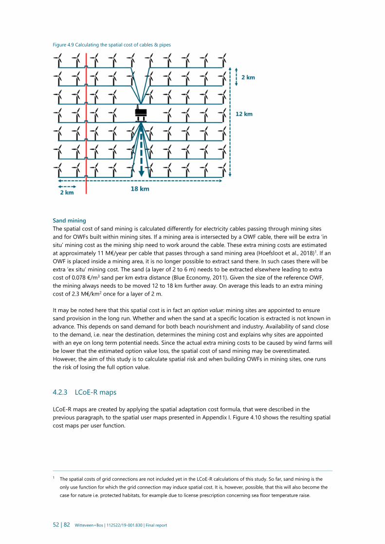
52 | 82 Witteveen+Bos | 112522/19-001.830 | Final report
Figure 4.9 Calculating the spatial cost of cables & pipes
Sand mining
The spatial cost of sand mining is calculated differently for electricity cables passing through mining sites
and for OWFs built within mining sites. If a mining area is intersected by a OWF cable, there will be extra ‘in
situ’ mining cost as the mining ship need to work around the cable. These extra mining costs are estimated
at approximately 11 M€/year per cable that passes through a sand mining area (Hoefsloot et al., 2018)1. If an
OWF is placed inside a mining area, it is no longer possible to extract sand there. In such cases there will be
extra ‘ex situ’ mining cost. The sand (a layer of 2 to 6 m) needs to be extracted elsewhere leading to extra
cost of 0.078 €/m3 sand per km extra distance (Blue Economy, 2011). Given the size of the reference OWF,
the mining always needs to be moved 12 to 18 km further away. On average this leads to an extra mining
cost of 2.3 M€/km2 once for a layer of 2 m.
It may be noted here that this spatial cost is in fact an option value: mining sites are appointed to ensure
sand provision in the long run. Whether and when the sand at a specific location is extracted is not known in
advance. This depends on sand demand for both beach nourishment and industry. Availability of sand close
to the demand, i.e. near the destination, determines the mining cost and explains why sites are appointed
with an eye on long term potential needs. Since the actual extra mining costs to be caused by wind farms will
be lower that the estimated option value loss, the spatial cost of sand mining may be overestimated.
However, the aim of this study is to calculate spatial risk and when building OWFs in mining sites, one runs
the risk of losing the full option value.
4.2.3 LCoE-R maps
LCoE-R maps are created by applying the spatial adaptation cost formula, that were described in the
previous paragraph, to the spatial user maps presented in Appendix I. Figure 4.10 shows the resulting spatial
cost maps per user function.
1 The spatial costs of grid connections are not included yet in the LCoE-R calculations of this study. So far, sand mining is the
only use function for which the grid connection may induce spatial cost. It is, however, possible, that this will also become the
case for nature i.e. protected habitats, for example due to license prescription concerning sea floor temperature raise.

53 | 82 Witteveen+Bos | 112522/19-001.830 | Final report
Figure 4.10 Individual spatial cost maps
Source: LCoE-R mapping model developed in this study
The range of the monetary value differs per user function, but the red colour always reflects the highest
value, while the green colour represents the lowest value1. For some user functions, such as small military
zones and protected habitats, there is hardly any variation in cost, because the cost depend on the presence
of the user function and not use intensity. For other users functions, such as large military zones, minor
shipping routes and fisheries there is much variation in cost. This variation is caused by difference in use
intensity. For example, for fisheries (bottom left) the costs are highest (red) where the most fishing activity
takes place, i.e. areas that are relatively frequently trawled.
The spatial risk costs (i.e. spatial adaptation costs) are added to the LCoE maps (see figure 4.5), to create
LCoE-R maps. Figure 4.11 shows the LCoE-R maps for the AC, DC and H&S connection type. In these three
LCoE-R maps, the spatial costs of the individual user maps are added up. This means that the costs of
multiple user functions at one location are included in the LCoE-R maps. It is remarked here, that the
cumulative spatial risk costs caused by clusters of OWFs are not included in the LCoE-R maps. Furthermore
the impact of spatial users shifting to another area and creating adaptation cost at the new location has not
been accounted for, as it is outside the scope of the study.
1 Colours are relative within one image and cannot be compared to the other images.
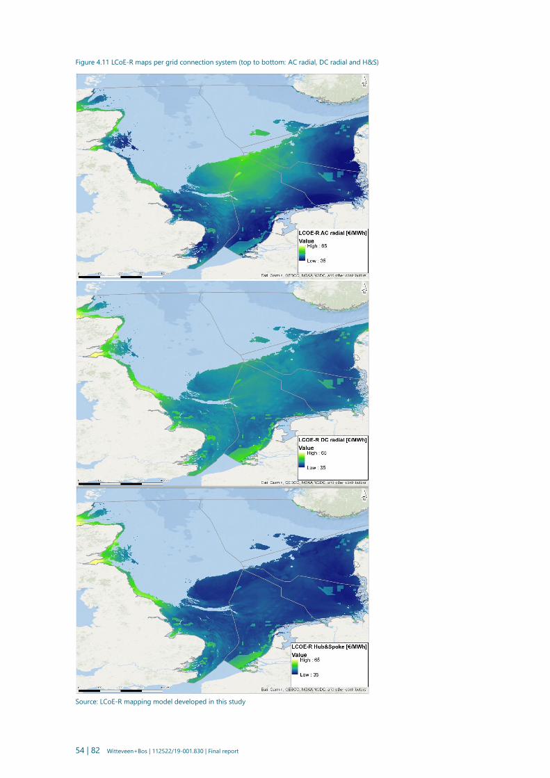
54 | 82 Witteveen+Bos | 112522/19-001.830 | Final report
Figure 4.11 LCoE-R maps per grid connection system (top to bottom: AC radial, DC radial and H&S)
Source: LCoE-R mapping model developed in this study

55 | 82 Witteveen+Bos | 112522/19-001.830 | Final report
In order to illustrate the difference between a LCoE map and a LCoE-R map, figure 4.12 shows both maps for
the H&S grid connection system.
Figure 4.12 LCoE (left) and LCoE-R (right) maps for the H&S grid connection system
Source: LCoE-R mapping model developed in this study
A visual inspection of both maps reveals that LCoE-R map has more green coloured areas near the Dutch
and English coast and at some distance of the German coast: these green areas have higher LCoE-R due to
the spatial planning risk of sand mining. The spatial planning risk of sand mining turns out to be the risk that
dominates all of the spatial planning risks in the levelized cost of energy, as the costs per km2 for the sand
mining function, seem to be the highest.

56 | 82 Witteveen+Bos | 112522/19-001.830 | Final report
5
IDENTIFYING POSSIBLE NEW OWF LOCATIONS
In this chapter possible new OWF locations for the period after 2030 are identified by means of the LCoE-(R)
mapping model that was described in the previous chapter. The mapping model has a drawing tool that
allows the user to draw new wind farms in the North Sea and immediately check the LCoE-R of both
individual farms and of a set of farms.
Three different identification perspectives are applied: an economic perspective (i.e. low LCoE-R), a visibility
perspective and a nature conservation perspective. This results in three different sets of possible new
locations. After checking the LCoE-(R) and the capacity of the three sets with possible new locations, a
preferred set is selected. For the preferred set a more detailed location specific grid connection will be
created in chapter 6. The preferred set with possible new locations is prepared for that purpose by reshaping
the OWFs to match the 1 GW size of the reference wind farm.
5.1 Searching for new locations from different perspectives
On the basis of the LCoE-R maps that were presented in figure 4.11 in chapter 4, three different sets of
possible new OWF locations were composed from three different perspectives:
1 low LCoE-R;
2 visibility from shore;
3 nature conservation.
The sets with possible new locations were composed, while keeping in mind that approximately 180 GW is
needed to decarbonize the power sector in the North Sea region. Given the already planned capacity of 75
(55 up to and 20 after 2030) GW in the baseline, sets with approximately 110 GW additional capacity are
strived for.
The grid connection system of each new location was determined as follows: AC was used for farms
nearshore (up to 80 km), DC for isolated farms far from shore (more than 80 km) and H&S for clustered
farms far from shore (more than 80 km). Some DC farms were selected in spite of their relatively high
LCoE-R. This was done in order to allow for extra analyses on the cost difference between the three different
grid connection systems at a later stage of this study.
5.1.1 Set with possible new locations based on low LCoE-R
The LCoE-R based set with possible new locations was created by visual inspection of the LCoE-R colour
maps of figure 4.11 in chapter 4. Polygons with a hosting capacity of approximately 1 GW were drawn in de
the dark blue areas of the colour maps. AC radial and H&S locations with a LCoE-R lower than approximately
45 €/MWh were included in the set. Since DC locations have a relatively high LCoE-R. Only three DC
locations were included. This was done to allow for a check on how DC locations influence the overall LCoE
of a grid roll-out path at a later stage of this study.

57 | 82 Witteveen+Bos | 112522/19-001.830 | Final report
The LCoE-R based search exercise resulted in a set of possible new locations with total capacity of 110 GW.
The locations of this set are presented as orange coloured polygons in figure 5.1. This figure also shows
baseline OWF locations, planned by national governments, up to and after 2030. These represent a total
capacity of approximately 75 GW.
Figure 5.1 Set with possible new locations based on low LCoE-R
Source: LCOE-R mapping model developed in this study
5.1.2 Set with possible new locations excluding visibility from shore
Visibility is an important aspect of offshore wind farms, that is not included in the spatial risk calculation and
therefore unaccounted for in the LCoE-R. Sullivan et al. (2013) and Crawford (2016) investigated the visibility
of wind farms. Their combined study results suggest that OWFs can:
- dominate the view up to 8 km from shore;
- be clearly visible up to 16 km from shore;
- be noticed by the casual observer up to 30 km from shore;
- be noticed by the concentrated observer up to 40 km from shore.
On the basis of this information, OWF locations were selected at a distance of more than 40 km from shore.
The choice was made to set the distance for Denmark at 20 km, since the threshold for being clearly visible is
less than 20 km and the Danish coast already has OWFs at less than 5 km from shore. This exercise resulted
in a set with possible new locations with a total capacity of 120 GW. Figure 5.2 shows the locations (in
orange) that are included in the visibility set.

58 | 82 Witteveen+Bos | 112522/19-001.830 | Final report
Figure 5.2 Set with possible new locations based on visibility exclusion
Source: LCOE-R mapping model developed in this study
5.1.3 Set with possible new locations excluding nature protected areas
The North Sea contains protected nature areas. A set of possible new OWF locations was created by drawing
OWF polygons in the dark blue areas of the LCoE-R colour map projected on a map with designated and
appointed nature areas. No polygons were drawn in the nature areas. This resulted in a set with possible new
locations with total capacity of 77 GW. The locations included are shown in figure 5.3.
The identified 77 GW is not sufficient to meet the Translate COP21 target of 180 GW. For that purpose an
additional capacity of 110 GW is needed. In chapter 7 a sensitivity analysis is carried out in relation to this:
extra OWFs adjacent to nature conservation areas are added (outside the dark blue areas) in order to
discover how the average LCoE-R is effected when the 180 GW target needs to be realized while
simultaneously avoiding the nature areas.

59 | 82 Witteveen+Bos | 112522/19-001.830 | Final report
Figure 5.3 Set with possible new locations based on nature exclusion
Source: LCoE-R mapping model developed in this study
5.2 Selection of a preferred set with possible new locations for grid roll-out
In table 5.1 the three sets of possible new OWF locations for the period after 2030 are compared for the sake
of selecting a preferred set for which a location specific grid roll-out path will be designed in chapter 6. In
order to provide a complete overview, table 5.1 also includes the baseline OWFs up to and after 2030, which
have already been planned by the national governments of the North Sea countries.
Table 5.1 Comparison of the three different sets with possible new locations
Set with possible new locations Number of
OWF
Surface
(km2)
Capacity (3.6
MW/km2)
(GW)
LCoE
(€/MWh)
LCoE-R
(€/MWh)
Baseline up to 2030 99 13,000 55* - -
Baseline planned after 2030 24 5,000 20** 39 40
LCOE-R based set 113 31,000 110 37 38
Visibility based set 130 34,000 120 37 38
Nature based set 87 21,000 77 38 38
OWF roll-out list after 2030 =
Baseline planned after 2030 +
LCOE-R based set
137 36,000 130 37 38
* The power density of these OWFs deviates from the power density of the reference farm which is 3.6 MW/km2.
** This capacity is recalculated for a power density of 3.6 MW/km2 ; see appendix I, table I.1.

60 | 82 Witteveen+Bos | 112522/19-001.830 | Final report
Table 5.1 show that the LCoE-R of the baseline planned after 2030 and of the three sets with possible new
locations ranges from 37 to 39 €/MWh. The LCoE-Rs are slightly higher and range from 38 to 40 €/MWh. It is
noted here that these LCoE ranges are numbers for the future (after 2030) that cannot be compared with the
today’s LCoEs nor with current bid prices or market values. The numbers strongly rely on multiple
assumptions that introduce uncertainties as described in table 4.1 in paragraph 4.1.4. The presented LCoEs
are merely meant to enable a comparison of locations.
A more detailed inspection of the numbers presented in table 5.1 shows that the visibility based set and the
nature based set of possible new locations have higher average LCoEs and LCoE-Rs than the LCoE-R based
set. This is due to those two sets containing relatively more wind farms further offshore. Locations further
from shore tend to have a higher LCoE and LCoE-R. The LCoE differences amount to 0.5 to 1.0 €/MWh for
respectively the visibility and nature based set. For the LCoE-R a comparable difference is found.
Such cost differences may seem small, but they need to be multiplied with the annual energy production to
see the actual cost difference that will occur every year during the 30 years of lifespan of the wind farm.
Multiplying these cost differences with the average annual energy production of 570 TWh1, reveals an extra
energy production cost (including spatial planning cost) of 250 M€/year million for visibility based and
440 M€/year for nature based, recurring every year for the next 30 years. Considering the extra cost to
society of the visibility and nature based sets of possible new locations, the LCoE-R based set is selected as a
basis for designing a grid roll-out pathway in chapter 6.
Impact of spatial planning risk
It is interesting to note that all three sets list were composed by taking spatial planning risk into account: the
selection was done on the basis of LCoE-R and not on the basis of LCoE. The average difference between the
LCoE and LCoE-R is 0.6 €/MWh. This means that the selected locations do have other user functions.
The cost difference of 0.6 €/MWh may seem little, but when taking into account a total annual energy
production of the OWFs after 2030 (130 GW) of 600 TWh/year2, the spatial planning risk costs add up to
360 M€/year for a period of 30 years.
Grid roll out list
Since the LCoE-R based set with possible new locations contains sufficient capacity and has the lowest
average LCoE-R, this set was selected for further grid design. Figure 5.4 shows the roll-out list, which
contains the possible new locations of the LCoE-R based set plus the planned OWF locations of the baseline
after 2030. The planned OWF locations up to 2030 are not included in the roll-out list, because this studies is
about offshore wind energy after 2030. In chapter 6 roll-out pathways will be developed for the locations
included in the roll-out list.
1 This is the average energy production (AEP) of the LCoE-R based set with possible new locations.. It is derived from the GIS
AEP-map.
2 This is the average energy production (AEP) of the roll-out list. It is derived from the GIS AEP-map.

61 | 82 Witteveen+Bos | 112522/19-001.830 | Final report
Figure 5.4 OWF roll-out list after 2030
Source: LCOE-R mapping model developed in this study

62 | 82 Witteveen+Bos | 112522/19-001.830 | Final report
6
GRID ROLL-OUT PATHWAYS
This chapter describes how different grid roll-out pathways were designed for the OWF roll-out list after
2030. In the first two paragraphs it is explained how inter-OWF wake losses were accounted for and how the
grid roll-out was optimized. In last two paragraphs the identified roll-out pathways are presented and a
preferred pathway is selected. It may be noted that in this chapter LCoE and not LCoE-R maps are the basis
of the calculations. The risk component was used to identify possible new locations, but is not needed to
design the offshore grid that connects these locations to the onshore grid.
6.1 Adding inter-OWF wake losses
So far, only wake losses inside the OWF were accounted for in the LCoE calculations. Now that the exact list
of OWF locations to be rolled out has been identified, inter-OWF wake losses can be included in order to
obtain a more accurate estimate of the overall LCoE.
ECN part of TNO performed an inter-OWF wake loss analysis, describing the wake loss that OWF locations
impose on each other. The results of this analysis show that four wake loss categories can be distinguished
based on the number of neighbouring OWFs which are aligned in the dominant wind direction: a single OWF
and a cluster of 2, 3 and more than 4 OWFs. Figure 6.1 illustrates this. The larger the cluster, the larger the
wake loss factor for that cluster. As a result:
- one isolated OWF has no additional wakes losses on top of internal wake losses;
- two OWFs clustered have 1.74 % additional wake losses on top of internal OWF wake losses;
- three OWFs clustered have 2.59 % additional wake losses on top of internal OWF wake losses;
- four OWFs clustered have 3.19 % additional wake losses on top of internal OWF wake losses.
Figure 6.1 Wind rose (left) and inter-OWF wake losses (right)
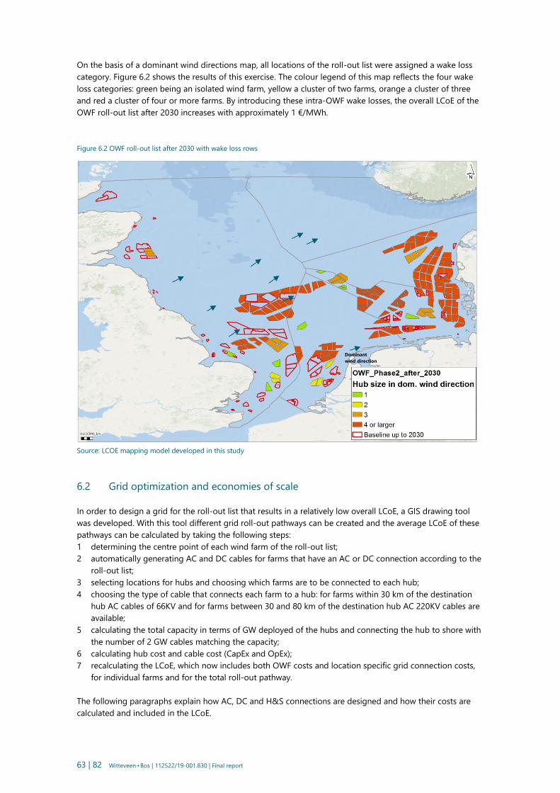
63 | 82 Witteveen+Bos | 112522/19-001.830 | Final report
On the basis of a dominant wind directions map, all locations of the roll-out list were assigned a wake loss
category. Figure 6.2 shows the results of this exercise. The colour legend of this map reflects the four wake
loss categories: green being an isolated wind farm, yellow a cluster of two farms, orange a cluster of three
and red a cluster of four or more farms. By introducing these intra-OWF wake losses, the overall LCoE of the
OWF roll-out list after 2030 increases with approximately 1 €/MWh.
Figure 6.2 OWF roll-out list after 2030 with wake loss rows
Source: LCOE mapping model developed in this study
6.2 Grid optimization and economies of scale
In order to design a grid for the roll-out list that results in a relatively low overall LCoE, a GIS drawing tool
was developed. With this tool different grid roll-out pathways can be created and the average LCoE of these
pathways can be calculated by taking the following steps:
1 determining the centre point of each wind farm of the roll-out list;
2 automatically generating AC and DC cables for farms that have an AC or DC connection according to the
roll-out list;
3 selecting locations for hubs and choosing which farms are to be connected to each hub;
4 choosing the type of cable that connects each farm to a hub: for farms within 30 km of the destination
hub AC cables of 66KV and for farms between 30 and 80 km of the destination hub AC 220KV cables are
available;
5 calculating the total capacity in terms of GW deployed of the hubs and connecting the hub to shore with
the number of 2 GW cables matching the capacity;
6 calculating hub cost and cable cost (CapEx and OpEx);
7 recalculating the LCoE, which now includes both OWF costs and location specific grid connection costs,
for individual farms and for the total roll-out pathway.
The following paragraphs explain how AC, DC and H&S connections are designed and how their costs are
calculated and included in the LCoE.
Dominant
wind direction

64 | 82 Witteveen+Bos | 112522/19-001.830 | Final report
In figure 6.3 the AC and DC farms of the roll-out list are connected to the onshore grid. They are connected
to the nearest landing point. The pink/fuchsia coloured lines reflect the AC cables, and the light green ones
the DC cables. Because the roll-out list contains more AC than DC farms, there are more pink/fuchsia
coloured lines than green ones.
Figure 6.3 Designing a grid for the roll-out list: the result of drawing in AC and DC radial connections
Source: LCoE mapping model developed in this study
The H&S-farms are connected directly to a hub with the intra-array cables. This is possible up to about
25-30 km from the OWF edge. In order to obtain economies of scale, hubs are located in such a way that the
number of OWFs, that can be directly connected to a hub, is maximized1.
Wind farms that are further than 30 km away from a hub can also be connected but require an AC substation
inside the farm. These substations are connected with 220 kV AC cables to the hub, while the farms are
connected with 66 kV cables to the AC substation. This new grid connection system is called AC hybrid. It is a
combination of AC radial and H&S2 that can be applied up to 80 km from the OWF edge. The reader is
referred forward to Figure 6.4 and 6.7 in paragraph 6.3.2 for a sketches of the AC hybrid system.
1 In essence, because the hub is typically at the centre of the connected OWFs.
2 It may be noted here that the energy loss of this AC hybrid GCS is currently not properly modelled, as it is still using the energy
loss of AC radial. Also for farms that are connected this way, OpEx is modelled on the basis of maintenance from the mainland
whereas it will actually take place from the hub. This means that the cost estimates for this connection type are not very
accurate as they are overestimated.

65 | 82 Witteveen+Bos | 112522/19-001.830 | Final report
Once all farms are connected to a hub, hub sizes in terms of GW and the required number of 2GW onshore
connections are known. While designing a grid roll-out pathway, a balance between short cable distances
and serving multiple countries is strived for. The onshore connection points for designing the grid roll-out
pathway are derived from a previous analysis that determined the spare capacity per onshore connection
point (Vree and Verkaik, 2017). It was assumed that these onshore connection points can handle the
connected OWFs’ electricity production and no further grid reinforcements were required.
In order to allow economies of scale to be achieved when designing grid roll-out pathways, the costs for the
hub foundation were varied, based on the hosting capacity of the hub and the applicable water depth
(depending on the location of the hub). This variation in costs allowed the analysis to apply hub sizes
ranging from 4-16 GW, thereby allowing hubs other than the initial 12 GW hub. Although large hubs have
higher costs than small hubs, the cost per GW are lower for large hubs than for small hubs, as large ones
host more OWFs. The hub costs used in this study were derived from a NSWPH consortium study1.
6.3 Identified roll-out pathways
Following the grid design procedure as explained in the previous paragraphs, two different roll-out pathways
were created from two different angles. The first angle was to simply create enough hubs to connect all
farms included in the roll-out list using 66 kV cables. The second angle was to reduce the number of hubs by
connecting more farms to one hub by means of the AC hybrid GCS and realise economies of scale. Figure 6.4
illustrates these two angles.
Figure 6.4 GCS concepts used to design roll-out pathways: without (top) and with (bottom) AC hybrid
1 In hub costs applied in this study pertained to hubs in the form of sandy islands.

66 | 82 Witteveen+Bos | 112522/19-001.830 | Final report
6.3.1 Pathway 1: Enough hubs
Figure 6.4 (top) shows a sketch of the grid connection system used to design a roll-out pathway with enough
hubs to connect all hub and spoke OWFs with a maximum distance of 30 km: the reach of the 66 kV cables.
Figure 6.5 shows the map in which all identified H&S farms are connected in this manner.
Figure 6.5 Pathway 1: Enough hubs1
Source: LCoE mapping model developed in this study
This pathway contains 17 hubs with a HVDC conversion capacity hosted by a single hub ranging from 3 to 8
GW. The average LCoE of this pathway is 40 €/MWh. This is higher than the average LCoE of the roll-out list
of 37 €/MWh that was presented in the previous chapter. The cost increase is a result of accounting for inter
wind farm wake losses and as a result of adding location specific grid connection costs. Figure 6.6 shows the
breakdown of the LCoE-results of this pathway.
1 As a first approximation for minimising grid integration cost, deeper inland connections have been considered which connect
offshore transmission cables to locations where available connection capacity is expected based on fossil fuel phase-out
scenarios.
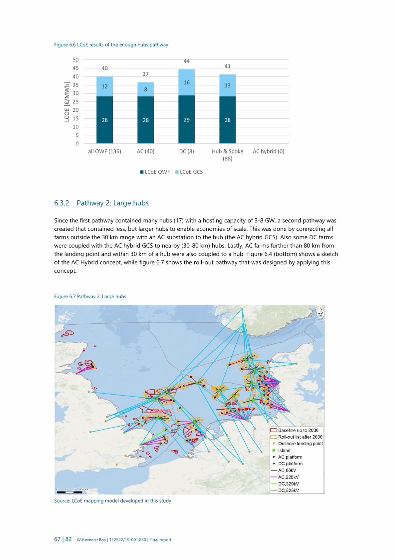
67 | 82 Witteveen+Bos | 112522/19-001.830 | Final report
Figure 6.6 LCoE results of the enough hubs pathway
6.3.2 Pathway 2: Large hubs
Since the first pathway contained many hubs (17) with a hosting capacity of 3-8 GW, a second pathway was
created that contained less, but larger hubs to enable economies of scale. This was done by connecting all
farms outside the 30 km range with an AC substation to the hub (the AC hybrid GCS). Also some DC farms
were coupled with the AC hybrid GCS to nearby (30-80 km) hubs. Lastly, AC farms further than 80 km from
the landing point and within 30 km of a hub were also coupled to a hub. Figure 6.4 (bottom) shows a sketch
of the AC Hybrid concept, while figure 6.7 shows the roll-out pathway that was designed by applying this
concept.
Figure 6.7 Pathway 2: Large hubs
Source: LCoE mapping model developed in this study
28 28 29 28
128
16 13
4037
4441
0
5
10
15
20
25
30
35
40
45
50
all OWF (136) AC (40) DC (8) Hub & Spoke(88)
AC hybrid (0)
LCO
E [€
/MW
h]
LCoE OWF LCoE GCS

68 | 82 Witteveen+Bos | 112522/19-001.830 | Final report
This pathway contains 11 hubs with a HVDC conversion capacity hosted by each hub ranging from 4 to
14 GW. Compared to the first path way, the number of hubs is reduced by 6, while the maximum hub
capacity is increased by 6 GW. The average LCoE of this pathway is 40 €/MWh. This is comparable to the
‘enough hubs’ pathway, but a more detailed inspection of LCoE breakdown reveals that the LCoE of the
‘large hubs’ pathway is approximately 0.4 €/MWh lower than the ‘enough hubs’ pathway. Figure 6.8 shows
the breakdown of the LCoE of this roll-out pathway.
Figure 6.8 LCoE results of the large hubs pathway
This LCoE breakdown shows that the farms connected with AC hybrid may themselves be relatively
expensive, but they reduce the overall LCoE of the roll-out pathway. This demonstrates that considering the
GCS of individual OWFs on a case by case basis may not yield the overall optimum cost for society. In order
to minimize the cost to society, the total expected roll out of both OWF and transmission assets should be
considered from an Internationally Coordinated Roll Out (ICRO) perspective.
6.3.3 Capturing economies of scale
The modest LCoE difference between the two presented pathways is an indication that there are economies
of scale to be gained by reducing the number and increasing the size of hubs. This hypothesis was tested by
adapting the grid design of three locations:
1 Dogger Bank: this location was selected since it contains the most hubs and consequently the potential
for realizing economies of scale by reducing the number of hubs seems large here;
2 Nord-Ost Passat and H2-20: for this location changing DC radial to AC hybrid could potentially capture
economies of scale;
3 Nearshore Denmark: two AC farms were changed to H&S and connected to the nearest hub to obtain
economies of scale.
Test location 1: Dogger Bank 5 to 3 hubs
The average LCoE at Dogger Bank is estimated to be 43 €/MWh for a grid design with 5 hubs of 4 to 6 GW.
By replacing the 5 small hubs on the Dogger Bank by 3 lager ones of 8, 10 and 12 GW, the average LCoE
drops with 1.0 €/MWh for this location. Apparently, the relatively expensive AC hybrid farms are out
weighted by the reduced hub costs.
28 28 29 28 30
11 815
11
18
4037
44
40
48
0
10
20
30
40
50
60
all OWF (136) AC (35) DC (3) Hub & Spoke (84) AC hybrid (14)
LCO
E [€
/MW
h]
LCoE OWF LCoE GCS

69 | 82 Witteveen+Bos | 112522/19-001.830 | Final report
Test location 2: DC radial changed to AC hybrid for Nord-Ost Passat and H2-20 (Germany Zone 5)
In pathway 1, the German OWFs Nord-Ost Passat and H2-20 were connected with DC. Figure 6.9 shows
these two locations. Their LCoEs were 46 and 47 €/MWh respectively. If one connects these locations with AC
hybrid, their LCoEs drop with 0.5 and 0 €/MWh respectively. This rather modest cost reduction suggests that
there are no significant economies of scale to be gained by coupling DC farms to nearby (30-80 km) hubs.
Figure 6.9 Nord-Ost Passat and H2-20 (left) and nearshore Denmark (right)
Source: LCoE mapping model & grid drawing tool developed in this study
Test location 3: AC radial changed to H&S nearshore Denmark
In pathway 1 there are three AC farms near the Danish shore that are within reach of a hub. By changing
their connection type to H&S and connecting them to this hub, the average LCoE of this Danish location
drops with 0.2 €/MWh, capturing a modest economies of scale advantage.
From the three test locations one can conclude that economies of scale can be realized by introducing larger
hubs and connecting as many as possible farms to these hubs. Connecting far from shore DC farms with a
relatively expensive AC hybrid system and/or connecting near shore AC farms also seems to generate
modest economies of scale advantages. Further testing where the optimum lies for the hosting capacity of
the hub can be done in a later stage of the NSWPH project.
6.4 Selection of preferred grid roll-out pathway
From the previous paragraphs it can be concluded that the identified grid roll-out pathway with large hubs
has a slightly lower LCoE compared to the pathway with enough hubs. Since this study focusses on costs
only, the ‘large hubs’ pathway is selected as a preferential pathway. Although this study focuses on the cost
factors of OWF locations, spatial planning as a whole needs to balance cost information with several other
tangible and intangible criteria. Hence, these other factors could influence the eventual optimum roll out
pathway.
The results of the economies of scale roll-out exercises suggest that pathways enabling economies of scale
by means of larger hubs that serve many farms, results in slightly lower overall LCoEs, even if the relatively
expensive AC hybrid grid connection system is applied.
For further optimization, increasing the hub size without having to use the AC hybrid type could be an
interesting option. There seem to be two different ways to realize this:
- by increasing the wind farm power density, so that more GW can be realized within 30 km of the hub;
- by investigating if 25-30 km is really the maximal distance for the direct connection to the hub via the
66 kV intra-array cables.
The sensitivity analysis in chapter 7.1 investigates the idea of increasing the power density of the wind farms.

70 | 82 Witteveen+Bos | 112522/19-001.830 | Final report
7
SENSITIVITY ANALYSES
In this chapter the results of three different sensitivity analyses are presented. The first analysis reveals the
potential for capturing economies of scale by increasing power density in combination with large hubs.
The second analysis shows how the LCoE is impacted if the H&S GCS is not used and all OWFs of the roll-out
list were to be connected with AC or with DC only. The third analysis presents what happens to the LCoE if
nature conservation areas are swapped by adjacent areas so that the amount of GW deployed is aligned with
the Paris i.e. The ‘Translate COP21’ target, while nature areas are excluded.
7.1 Sensitivity to wind farm power density
The key question of this sensitivity analysis is ‘What happens to the LCoE if a higher wind farm power density
is applied? ‘ In order to find the answer to this question a test location in the German Zone 4 was selected,
since the German OWFs are currently developed with a power density range of 10 to 17 MW/km2, which is
significantly higher than the 3.6 MW/km2 of the reference farm of this study. Figure 7.1 shows the test
location: Zone 4 North hub and its surrounding H&S farms.
Figure 7.1 Test location for power density with grid connection H&S)
Source: LCoE mapping model & grid drawing tool developed in this study
In order to redesign the test location with higher power densities, the farms were ‘unclustered’ to undo the
previous design that used a reference power density of 3.6 MW/km2. Subsequently, the capacity of each
polygon was calculated in terms of MW with higher densities of 6.4 and 14.4 MW/km2. On the basis of these
capacities the locations were clustered again into farms of approximately 1 GW. Since different power
densities have different wake losses, the annual energy production was recalculated while taking into
account the relevant losses. Table 7.1 shows the wake loss factors in relation to power density that were used
in this calculation.

71 | 82 Witteveen+Bos | 112522/19-001.830 | Final report
Table 7.1 Wake losses for different OWF power densities compared to an isolated reference farm
Turbine distance expressed in rotor diameter D 8D 6D 4D
density (MW/km2) 3.6 6.4 14
1 OWF 0.0 % (reference) +1.3 % +7.9 %
2 OWF cluster +1.7 % +4.5 % +11 %
3 OWF cluster +2.6 % +5.6 % +12 %
≥4 OWF cluster +3.2 % +6.4 % +14 %
Source: ECN part of TNO, 2018
After recalculating the annual energy production, the farms were connected to the new, larger, hubs.
The OWF and hub locations were not changed. In other words: only the size of the hub was altered, not the
location, so the hub size impact can be isolated. Finally, the number of cables from the hub to the shore was
increased to match the new hub capacity. Subsequently, the LCoE was recalculated. Figure 7.2 shows the
results of this experiment.
Figure 7.2 Sensitivity of LCoE to farm power density
Figure 7.2 shows that applying higher power densities without taking the economies of scale advantage of
hub size into account, would- of course- only increase the LCoE. But when these economies of scale are
accounted for the LCoE is reduced (with 1.5 and 0.4 €/MWh for densities of 6.4 and 14.4 MW/km2
respectively) in spite of the fact that wake losses are higher at higher power densities.
Figure 7.2 also suggests that there is an optimal power density between 3.6 (8D) and 14.4 MW/km2 (4D), as
the LCoE realized with a power density of 14.4 MW/km2 (4D) of 43 €/MWh is 1.1 €/MWh higher than the
LCoE realized with a power density of 6.4 MW/km2 (6D), but 0.4 €/MWh lower than the LCoE with a power
density of 3.6 MW/km2 (8D).
29 30 30 32 32
14 15 1216
10
43 4542
48
43
0
10
20
30
40
50
60
8D spacing,baseline
6D spacing, incl.add. wake loss
6D spacing, incl.add. wake loss
and islandeconomies
4D spacing, incl.add. wake loss
4D spacing, incl.add. wake loss
and islandeconomies
LCO
E [€
/MW
h]
LCoE OWF LCoE GCS

72 | 82 Witteveen+Bos | 112522/19-001.830 | Final report
On the basis of these results it is concluded that hub economies of scale, based on sandy island hubs, seem
to surpass wake loss diseconomies of scale. This means that using a reference farm with a higher power
density (than 3.6 MW/km2), e.g. more comparable power densities as used in German farms, may further
reduce the LCoE, while at the same time it reduces the space consumption of offshore wind farms and
thereby also spatial planning conflicts. Further analysis is required to determine the optimum OWF power
density and to reveal the tipping point of where the impact of wake losses becomes dominant.
7.2 Sensitivity to no hubs
The LCoE breakdowns of the ‘Enough hubs’ and ‘Large hubs’ roll out pathways show that the average LCoE
of H&S locations is higher than the average of AC locations but lower than the average LCoE of DC locations.
A more detailed inspection of the LCoEs of individual AC, DC and H&S locations, however, reveals that the
LCoE range of the different grid connection systems have much overlap. This evokes the question of what
the LCoE of the roll-out list would be, when no hubs are used. In other words: ‘what if all newly identified
locations are connected with just AC or DC, and no hubs are applied?’ In order to answer this question all
farms of the roll-out list with a H&S GCS were changed into farms using the DC radial GCS, while the
AC-locations were not changed. Subsequently the LCoE was recalculated.
This pathway is comparable with the NIRO scenario, as defined in the Urgency and Benefit study (Vree and
Verkaik, 2017). In this scenario no hubs are applied and the OWFs are connected radially to the nearest
onshore grid connection point. As such, in this scenario it is allowed to connect an OWF that is developed in
another country’s EEZ. To enable this, strong international coordination is needed.
Figure 7.3 shows the roll-out design of the ‘no hubs’ pathway.
Figure 7.3 Grid roll-out pathway without hubs
Source: LCoE-mapping model developed in this study
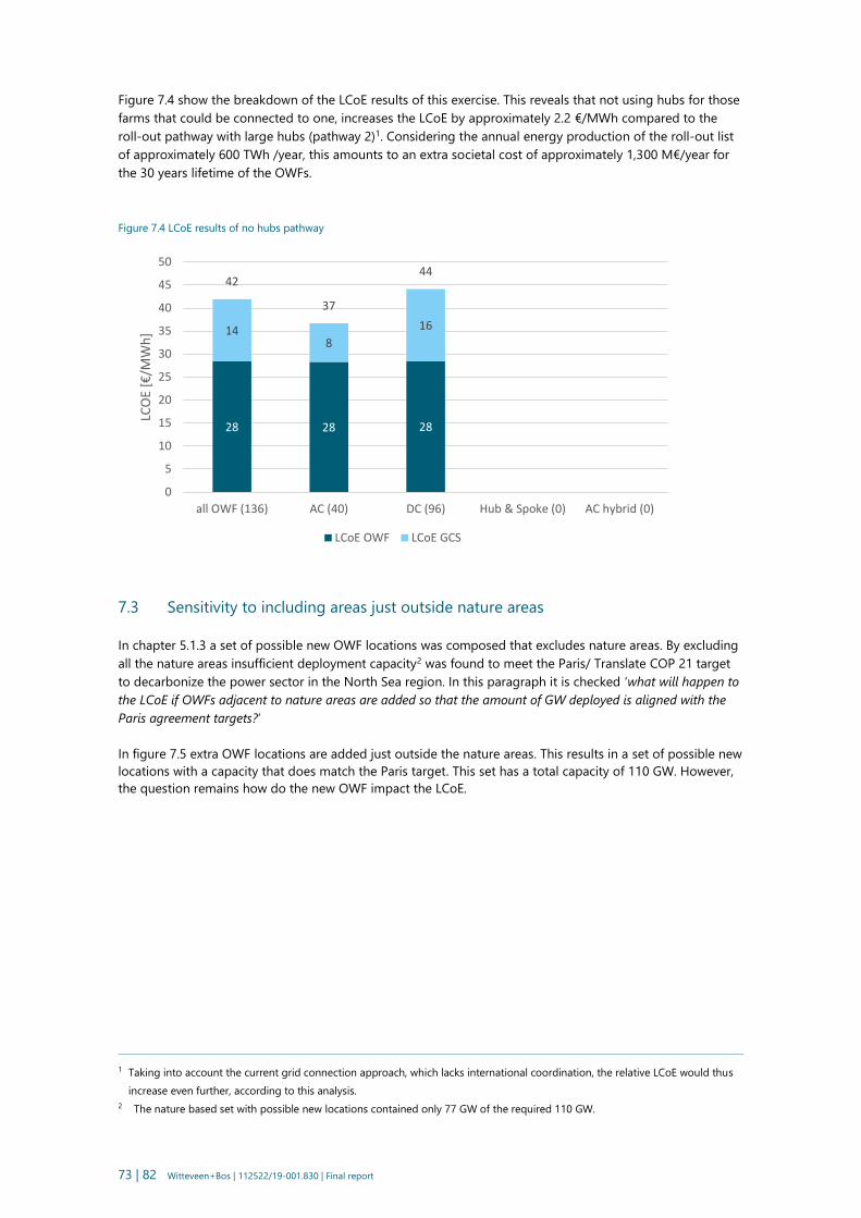
73 | 82 Witteveen+Bos | 112522/19-001.830 | Final report
Figure 7.4 show the breakdown of the LCoE results of this exercise. This reveals that not using hubs for those
farms that could be connected to one, increases the LCoE by approximately 2.2 €/MWh compared to the
roll-out pathway with large hubs (pathway 2)1. Considering the annual energy production of the roll-out list
of approximately 600 TWh /year, this amounts to an extra societal cost of approximately 1,300 M€/year for
the 30 years lifetime of the OWFs.
Figure 7.4 LCoE results of no hubs pathway
7.3 Sensitivity to including areas just outside nature areas
In chapter 5.1.3 a set of possible new OWF locations was composed that excludes nature areas. By excluding
all the nature areas insufficient deployment capacity2 was found to meet the Paris/ Translate COP 21 target
to decarbonize the power sector in the North Sea region. In this paragraph it is checked ‘what will happen to
the LCoE if OWFs adjacent to nature areas are added so that the amount of GW deployed is aligned with the
Paris agreement targets?’
In figure 7.5 extra OWF locations are added just outside the nature areas. This results in a set of possible new
locations with a capacity that does match the Paris target. This set has a total capacity of 110 GW. However,
the question remains how do the new OWF impact the LCoE.
1 Taking into account the current grid connection approach, which lacks international coordination, the relative LCoE would thus
increase even further, according to this analysis.
2 The nature based set with possible new locations contained only 77 GW of the required 110 GW.
28 28 28
148
16
42
37
44
0
5
10
15
20
25
30
35
40
45
50
all OWF (136) AC (40) DC (96) Hub & Spoke (0) AC hybrid (0)
LCO
E [€
/MW
h]
LCoE OWF LCoE GCS

74 | 82 Witteveen+Bos | 112522/19-001.830 | Final report
Figure 7.5 A set of possible new locations based on nature exclusion after adding additional OWFs
Source: LCoE-R mapping model developed in this study
In order to answer this question two grid roll-out pathways were designed for the new nature exclusion
based set of possible new locations:
- one with simply enough hubs to connect each farms;
- one with less, but larger hubs.
This is similar to the analysis done in section 6.3. Figures 7.6 and 7.8 show these two roll-out pathways, while
figures 7.7 and 7.9 show the breakdowns of their respective LCoEs.
Figure 7.6 Grid roll-out pathway for the ‘outside nature areas’ set with enough hubs
Source: LCoE-mapping model developed in this study

75 | 82 Witteveen+Bos | 112522/19-001.830 | Final report
Figure 7.7 LCoE results of the ‘outside nature areas’ set with enough hubs pathway
Figure 7.8 Grid roll-out pathway for the ‘outside nature areas’ set with large hubs
Source: LCoE-mapping model developed in this study
29 29 28 29
138
1813
41
37
46
42
0
5
10
15
20
25
30
35
40
45
50
all OWF (141) AC (30) DC (12) Hub & Spoke (99) AC hybrid (0)
LCO
E [€
/MW
h]
LCoE OWF LCoE GCS

76 | 82 Witteveen+Bos | 112522/19-001.830 | Final report
Figure 7.9 LCoE results of the ‘outside nature areas’ set with large hubs pathway
Table 7.2 briefly summarizes the results of this sensitivity analysis in such a way that the cost consequences
of adding nature adjacent areas are revealed.
Table 7.2 The cost impact of meeting the Translate COP21 target while excluding nature areas at the same time
Roll-out
design
LCoE without nature adjacent
locations to realise sufficient
capacity
LCoE with extra nature adjacent
locations to realise sufficient capacity
Extra cost due extra
nature areas in M€/year*
enough
hubs
40 41 730
large hubs 40 41 680
* Given an annual energy production of the roll-out list of approximately 600 TWh/year and LCoE-numbers that were not rounded.
From table 7.2 it can be concluded that adding extra nature adjacent areas, to realize sufficient capacity to
meet the Translate COP21 target, induces an extra societal cost of approximately 680 to 730 M€/year for the
30 year lifespan of the OWFs. This cost increase is primarily driven by the facts that the OWFs are ‘moved’ to
deeper waters and that the new OWFs are less clustered and thus capture less economies of scale.
Table 7.2 also shows that pathways without nature adjacent areas yield a roll-out LCoE of approximately
40 €/MWh, while pathways with such areas have a LCoE that is approximately 1 €/MWh higher. This LCoE
increase is caused by higher OWF costs as well as higher offshore transmissions cost per MWh of the added
nature adjacent locations.
These results demonstrate that there are choices to be made in spatial planning of OWF locations. Avoiding
nature areas could increase the LCoE of large scale OWF deployment and subsequently the cost to society of
reaching the Paris Agreement climate goals.
29 29 29 29 30
128
1612
19
4137
4540
49
0
10
20
30
40
50
60
all OWF (141) AC (27) DC (6) Hub & Spoke (94) AC hybrid (14)
LCO
E [€
/MW
h]
LCoE OWF LCoE GCS

77 | 82 Witteveen+Bos | 112522/19-001.830 | Final report
8
MAIN RESULTS & FOLLOW UP STUDIES
This chapter provides an overview of the main results of this study and makes some suggestions for follow
up studies.
8.1 Main results
The main results of this study are possible new OWF locations in the North Sea and their LCoEs, two different
grid rollout pathways and their LCoEs plus the results of sensitivity analyses on not applying the H&S grid
connection type and on including OWF locations adjacent to nature areas.
8.1.1 Possible new OWF locations and their LCoEs
In this study possible new OWF locations for the period after 2030 were identified using LCoE-R maps.
The identified new locations had a total capacity of 110 MW. Together with the already planned baseline
locations after 2030 of 20 MW, they form a roll-out list of 130 GW. Figure 8.1 shows a map with the OWF
locations of the roll-out list (orange polygons) and the locations of the baseline up to 2030 (red polygons).
The baseline farms up to 2030 represent a total capacity of 46 GW, assuming a power density of
3.6 MW/km2.
Figure 8.1 Roll-out list and baseline up to and after 20301
Source: LCOE-R mapping model developed in this study
1 OWF areas depicted in this figure provides a point of departure to stimulate discussion among various stakeholders and do not
represent any specific policy recommendation.
78 | 82 Witteveen+Bos | 112522/19-001.830 | Final report
The most attractive locations in terms of LCoE are at Borkum Riffgrund (36 €/MWh), facing the Danish coast
(37 €/MWh), the Dutch coast (38 €/MWh), at East Anglia, the Eastern German coast, the Jyske Rev plus to the
North of the Wadden (39 €/MWh), at the North Norfolk sandbanks (41 €/MWh) and also at the Doggersbank
(42 €/MWh)1. It is noted here that the LCoEs are numbers for the future that cannot be compared with
today’s LCoEs.
8.1.2 Roll-out pathways and their LCoE
The OWFs of the roll-out list were connected to the grid with two different design strategies: a pathway with
enough hubs to serve all the identified farms and one with large hubs in order to capture hub economies of
scale. Both roll-out pathways turned out to have an average LCoE of 40 €/MWh, but a detailed inspection of
the LCoE breakdowns of both pathways showed that the ‘large hubs’ pathway has a slightly lower average
LCoE than the ‘enough hubs’ pathway due to lower grid connection cost.
For the roll-out pathway with enough hubs, it was found that the majority of farms had a LCoE between 37
and 45 €/MWh. The more expensive farms were DC farms. In this pathway most hubs could only serve 4 to
6 farms due the limited connection distance of 30 km, which is caused by 66 kV AC cable technology
constraints.
The pathway with large hubs was designed to capture economies of scale of hub size. In order to capture
these, the limited hub connection distance needed to be increased. For this purpose a new GCS was
introduced: AC hybrid. With the AC hybrid concept it becomes possible to design a roll-out pathway with
larger hubs serving 8 to 10 farms. Even though the few OWFs that require an AC hybrid connection are
relatively expensive (46-49 €/MWh), they allow the majority of farms to shift to a relatively low LCoE-range
(37-40 €/MWh). This shift reduces the average LCoE of the whole roll-out list. The attempt to capture
economies of scale with the large hubs pathway that included AC hybrid farms, resulted in a modest average
LCoE reduction of 0.4 €/MWh compared to the enough hubs pathway.
8.1.3 Sensitivity analyses
In sensitivity analyses additional roll-out pathways were designed to answer the following two questions:
- What if no hubs are applied and farms with a H&S GCS are connected via a DC GCS instead2?
- What if nature areas are excluded and extra OWF locations are added outside nature areas to meet Paris
Agreement/Translate COP21 target of 180 GW?
Figure 8.2 shows that not applying the H&S GCS (no hubs) increases the LCoE with 2 €/MWh. This figure also
shows that excluding nature areas while realising sufficient capacity increases the LCoE with 1 €/MWh in
both a grid roll-out pathway with enough hubs and with large hubs.
1 This ranking shows that Doggersbank does not have the lowest levelized cost per MWh. This is caused by the fact that the UK
baseline farms at the Doggersbank are not connected to the hub, which limits the economies of scale of the hub.
2 AC is not considered as this more costly for farms further offshore than DC.

79 | 82 Witteveen+Bos | 112522/19-001.830 | Final report
Figure 8.2 Comparison of all grid roll-out pathways
8.2 Follow-up studies
This paragraph discusses topics which should be further investigated in follow up studies, because there
exists an information gap and/or they could significantly influence the LCoE. The topics pertain to spatial risk,
economies of scale and interconnection benefits.
8.2.1 More detailed investigation of spatial risks
All spatial risks, i.e. all spatial user functions, that were included in this study deserve extra detailing in order
to get a more accurate estimate of spatial planning risk cost i.e. adaptation costs. For two crucial functions,
nature and shipping, some practical suggestions for follow up work are discussed here.
Birds
Two different types of birds need to be considered: migratory birds and sea birds. While investigating the
spatial planning risk of migratory birds, it was discovered that North Sea covering maps with bird migration
routes are not available. These are needed in order to properly estimate the number of shut down hours per
year for the possible new farm locations. Without this information one could identify new locations that turn
out not be attractive due lost energy production. Additionally, evidence was found suggesting that the
shutdown threshold is likely to be increased in the future, possibly resulting in a significant effect on the
LCoE. Another aspect that could be taken into account in follow up work on this topic is the possible impact
of hub islands on migratory routes.
While determining sea bird risks, information on effective mitigation measures for sea birds turned out to be
missing. OWFs may induce a loss of habitat, reducing sea birds’ foraging area. Such losses need to be
compensated in order not to jeopardize healthy population sizes. Consequently, follow up work on effective
mitigation measures for sea birds is needed.
Shipping corridor design
During this study it was difficult to create a monetary trade-off between creating a shipping corridor
allowing ships to pass through an OWF versus having ships sail around OWFs inducing detour cost. This
requires detailed information on shipping densities (including frequencies and vessel types) plus a detailed
design of international passages through clusters of OWFs. Appendix III gives an example of a detailed
shipping corridor design for planned German farms. A follow up study on this topic could enhance smart
corridor designs that limit spatial planning cost and consequently lower the LCoE-R. It can also help to
obtain more accurate estimates of the spatial planning costs concerning shipping.
28 28 28 29 29
14 12 11 13 12
42 40 40 41 41
0
5
10
15
20
25
30
35
40
45
No hubs Enough hubs Large hubs Outside natureenough hubs
Outside naturelarge hubs
LCO
E [€
/MW
h]
LCoE OWF LCoE GCS
2 1 1

80 | 82 Witteveen+Bos | 112522/19-001.830 | Final report
8.2.2 Economies and diseconomies of scale
In this study it was found that the H&S GCS has economies of scale which can be further increased by
increasing the wind farm power density. A higher power density means that more GW can be connected to a
single hub. Increasing wind power density, however, also introduces diseconomies of scale due to wake
losses. In this study additional wake losses at higher power densities were simulated for OWF clusters up to
4 GW. Consequently, two types of follow up work seem relevant:
- research on hub (island) cost in relation to hub size and power density to enable a more accurate
quantification of economies of scale of hubs;
- research on wake losses for clusters larger than 4 GW to enable a correct quantification of the
diseconomies of scale due to wake loss.
8.2.3 Include interconnection benefits
This study reveals that the H&S GCS can lower the average LCoE of offshore wind energy production.
The fact that a hub is connected with spokes to multiple countries enables two additional benefits that were
not quantified in this study:
- interconnection trading between countries can lead to both energy bill savings for consumers and higher
profits for producers since energy demand and supply become more synchronized;
- compared to traditional AC and DC radial GCSs, the H&S GCS can help the energy transition by reducing
the amount of required grid reinforcements and the energy storage capacity. This can save costs.
In order quantify these benefits it is suggested to upgrade the LCoE mapping model that was developed in
this study with a real time energy trading simulation and to add grid reinforcement and storage costs to the
cost calculations of the model.
81 | 82 Witteveen+Bos | 112522/19-001.830 | Final report
9
REFERENCES
Literature
1 Blue Economy (2011). Financial impacts sand extraction strategy- price components, Blue Economy
commissioned by the Ministry of Infrastructure and Environment, Agency of Water, Rijswijk.
2 Bulder, B.H., E.T.G. Bot, G. Bedon, (2018). Optimal wind farm power density analysis for future offshore
wind farms, ECN part of TNO commissioned by the Ministry of Economic Affairs of the Netherlands.
3 Crawford, M. (2016). What Empirical Research has Established about Wind Farm Visual Impact, S.N., S.L.
4 Dubois, C. (2013). Bat mortality check and bat monitoring in the Perwez wind farm, CSD Ingenieurs
commissioned by Aspiravi S.A., Namur.
5 EZK, (2018). Kamerbrief- Routekaart windenergie op zee 2030. Minister van Economische Zaken en
Klimaat, Den Haag.
6 Gerrits, S. (2017). Feasibility Study of the Hub and Spoke Concept in the North Sea, s.n., s.l..
7 Hoefsloot, N., M. de Pater, E.C.M. Ruijgrok, d. van Gent, I. Laane, R. v.d. West, W. Gotje, (2018). Integral
cost-benefit study roadmap offshore wind energy, Decisio & Witteveen+Bos commissioned by the
Ministry of Economic Affairs and Climate, The Hague.
8 Hoefsloot, N., M. de Pater, G. van der Meulen, (2010). Socio-economic cost effectivity of spatial options
for offshore wind energy; SE-CEA Wind energy North Sea, Decisio commissioned by the Ministry of
Traffic and Water, The Hague.
9 Hoefsloot, N., M. de Pater, M. Wijnen, D. van Gent, R. Abma, E.C.M. Ruijgrok, (2014). SC-CBA wind energy
within the 12-mile zone, Decisio & Witteveen+Bos commissioned by the Ministry of Economic Affairs,
The Hague.
10 Hundleby, G. and K. Freeman, (2017). Unleashing offshore wind potential, BVG Associates commissioned
by Wind Europ, s.l.
11 IEA, (2013). Technology Roadmap - Wind energy - 2013 edition. International Energy Agency, Den Haag.
12 ICES, (2017). The greater North Sea Ecoregion- Fisheries Overview, International Council for the
Exploration of the Sea (ICES), Copenhagen.
13 Jongbloed, R.H., J.T. van der Wal, H.J. Lindeboom, (2014). Identifying space for offshore wind energy in
the North Sea; Consequences of scenario calculations for interactions with other marine uses, Energy
Policy, 68: 320–333.
14 Kamp, H.G.J.(2016). Decision lot I wind energy location Holland Coast (south), the Ministry of Economic
Affairs, published in: Government Gazette, nr. 111, The Hague.
15 Klomp, W., C. Hoyng, P. de Vries, (2017). North Sea Wind Power Hub Technical and financial feasibility
study final report, Royal Haskoning DHV, Amersfoort.
16 Krijgsveld, K.L., R.C. Fijn, R. Lensink, (2015). Occurrence of peaks in songbird migration at rotor heights of
offshore wind farms in the southern North Sea, Bureau Waardenburg, Culemborg.
17 Lengkeek, W., K. Didderen, M. Teunis, F. Driesen, J.W.P. Coolen, O.W. Bos, S.A. Vergouwen, T.C.
Raaijmakers, M.B. de Vries, M. van Koningsveld, (2017). Eco-friendly design of scour protection: potential
enhancement of ecological functioning in offshore wind farms; Towards an implementation guide and
experimental set-up, Deltares, WUR and Bureau Waardenburg, Delft.
18 Leopold, M.F. , M. Boonman, M.P. Collier, N. Davaasuren, R.C. Fijn, A. Gyimesi, J. de Jong, R.H. Jongbloed,
B. Jonge Poerink, J.C. Kleyheeg-Hartman, K.L. Krijgsveld, S. Lagerveld, R. Lensink, M.J.M. Poot, J. Tjalling
van der Wal, M. Scholl, (2014). A first approach to deal with cumulative effects on birds and bats of
offshore wind farms and other human activities in the Southern North Sea, Imares, Wageningen.

82 | 82 Witteveen+Bos | 112522/19-001.830 | Final report
19 Limpens, H.J.G.A., S. Lagerveld, I. Ahlén, D. Anxionnat, T. Aughney, H.J. Baagøe, L. Bach, P. Bach, J.P.C.
Boshamer, K. Boughey, T. Le Campion, M. Christensen, J.J.A. Dekker, T. Douma, M.-J. Dubourg-Savage, J.
Durinck, M. Elmeros, A.-J. Haarsma, J. Haddow, D. Hargreaves, J. Hurst, E.A. Jansen, T.W. Johansen, J. de
Jong, D. Jouan, J. van der Kooij, E.-M. Kyheroinen, F. Mathews T.C. Michaelsen, J.D. Møller, G. Pētersons,
N. Roche, L. Rodrigues , J. Russ, Q. Smits , S. Swift, E.T. Fjederholt, P. Twisk, B. Vandendriesche,
20 M.J. Schillemans, (2017). Migrating bats at the southern North Sea - Approach to an estimation of
migration populations of bats at southern North Sea, Rapport 2016.031. Zoogdiervereniging (Dutch
Mammal Society), Nijmegen and Wageningen Marine Research.
21 Matthijsen, J., E. Dammers and H. Elzenga, (2018). The future of the North Sea; The North Sea in 2030 and
2050: a scenario study, PBL (Planbureau voor de Leefomgeving),The Hague.
22 Müller, M., E. Haesen, L.Ramaekers, N.Verkaik, (2017). Translate COP21; 2045 outlook and implications for
offshore wind in the North Seas, Ecofys, commissioned by TenneT and Energinet.dk, Utrecht.
23 Remy, T., A. Mbistrova, I. Pineda, (2018). Offshore Wind in Europe - Key trends and statistics 2017, Wind
Europe, Brussels.
24 Romijn, G., P. Verstraten, H. Hilbers, A. Brouwers, (2016). Freight transport and Sea harbours, Welfare and
Environment, Scenario study for 2020 and 2050; back ground document, Central Planning Agency, The
Hague.
25 Sullivan, R.G. L.B. Kirchler, J. Cothren and S.L. Winters, (2013). Offshore Wind Turbine Visibility and Visual
Impact Threshold Distances, Environmental Science Division, Argonne National Laboratory, Argonne,
Illinois, USA.
26 Van der Tak, C., (2009). Traffic impact of wind farms, Marin commissioned by the Ministry of
Infrastructure and Environment, Agency of Water, The Hague.
27 Van der Tak, C., (2010). Quantitative risk assessment for offshore wind farms in the North Sea, Marin
commissioned by the Ministry of Transport, Public Works and Water Management, Wageningen.
28 Van Oostenbrugge, H. D. Slijkerman, K. Hamon, O. Bos, M. Machiels, O. van de Valk, N. Hintzen, E. Bos, J.
Tjalling van der Wal, J. Coolen, (2015). Effects of seabed protection on the Frisian Front and Central
Oyster Grounds; A cost benefit analysis, Wageningen University and Research Centre, Wageningen.
29 Vree B., N. Verkaik, (2017). North Sea Infrastructure - Urgency and Benefits; Cost reduction opportunities
through regional coordination, Ecofys, Utrecht.
30 Vree, B., N. Verkaik, M. Goher-ur-Rehman, (2017). A comparative LCOE analysis of a national incremental
and international coordinated roll-out for the Dutch Dogger Bank area, Ecofys, Utrecht.
Websites
1 www.rwseconomie.nl (=website Ministry of Waterways): cost barometer Deep Sea Shipping, (2016).
2 https://www.ncdc.noaa.gov/data-access/model-data/model-datasets/climate-forecast-system-version2-
cfsv2 (=website National Oceanic and Atmospheric Administration, NOAA): climate forecast system,
(2018).
Maps and GIS data
1 Emodnet, (2017). GIS shapefiles EMODnet Human Activities, Environment, Natura 2000, update 'Natura
2000 End 2017', by the EEA in 2018, downloaded from www.emodnet-humanactivities.eu/search-
results.php?dataname=Natura+2000.
2 TenneT TSO GmbH, (2018). GIS shapefiles for German offshore wind farms.
3 UNEP/GRID-Arendal, (2015). Cartograph Riccardo Pravettoni, downloaded from
www.grida.no/resources/7643.
4 Wageningen Marine Research, IMARES, (2014). GIS shapefiles for North Sea covering user functions.

Appendices


Witteveen+Bos | 112522/19-001.830 | Appendix I | Final report
I
APPENDIX: TRENDS IN SPACE USE OF THE NORTH SEA
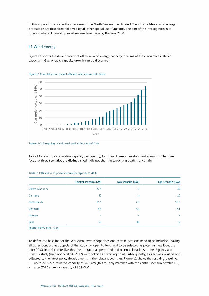
Witteveen+Bos | 112522/19-001.830 | Appendix I | Final report
In this appendix trends in the space use of the North Sea are investigated. Trends in offshore wind energy
production are described, followed by all other spatial user functions. The aim of the investigation is to
forecast where different types of sea use take place by the year 2030.
I.1 Wind energy
Figure I.1 shows the development of offshore wind energy capacity in terms of the cumulative installed
capacity in GW. A rapid capacity growth can be discerned.
Figure I.1 Cumulative and annual offshore wind energy installation
Source: LCoE mapping model developed in this study (2018)
Table I.1 shows the cumulative capacity per country, for three different development scenarios. The sheer
fact that three scenarios are distinguished indicates that the capacity growth is uncertain.
Table I.1 Offshore wind power cumulative capacity to 2030
Central scenario (GW) Low scenario (GW) High scenario (GW)
United Kingdom 22.5 18 30
Germany 15 14 20
Netherlands 11.5 4.5 18.5
Denmark 4.3 3.4 6.1
Norway - - -
Sum 53 40 75
Source: (Remy et.al., 2018)
To define the baseline for the year 2030, certain capacities and certain locations need to be included, leaving
all other locations as subjects of the study, i.e. open to be or not to be selected as potential new locations
after 2030. In order to realize this, the operational, permitted and planned locations of the Urgency and
Benefits study (Vree and Verkaik, 2017) were taken as a starting point. Subsequently, this set was verified and
adjusted to the latest policy developments in the relevant countries. Figure I.2 shows the resulting baseline:
- up to 2030 a cumulative capacity of 54.8 GW (this roughly matches with the central scenario of table I.1);
- after 2030 an extra capacity of 25.9 GW.

Witteveen+Bos | 112522/19-001.830 | Appendix I | Final report
This adds up to total amount of 74.3 GW deployed in the baseline. In this spatial study the amount of 54.8
GW is considered to be a fixed amount. The extra of 25.9 GW is adapted to the (lower) wind power density of
the reference farm used in this study: this means that it stands for 19.5 GW.
Figure I.2 Offshore wind energy reference map
Source: adapted from Vree and Verkaik, (2017)
I.2 Military use
Of course the military situation in 2030 is unknown. Military zones are, however, rarely moved and the
situation in 2030 is not expected to be much different from today. Possibly the recent American demands for
Europe to increase military defence expenditure might result in an expansion of practice zones. It might just
as well lead to extra investments in military equipment or to more expenses on military interventions in
conflict zones. Given the lack of clear indications, the military zone map of IMARES (Jongbloed et al, 2014) is
used to create a reference map that shows whether or not a location used for military purposes. Figure I.3
shows this reference map.
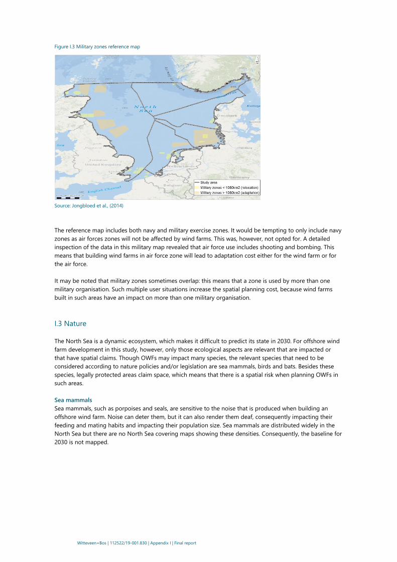
Witteveen+Bos | 112522/19-001.830 | Appendix I | Final report
Figure I.3 Military zones reference map
Source: Jongbloed et al., (2014)
The reference map includes both navy and military exercise zones. It would be tempting to only include navy
zones as air forces zones will not be affected by wind farms. This was, however, not opted for. A detailed
inspection of the data in this military map revealed that air force use includes shooting and bombing. This
means that building wind farms in air force zone will lead to adaptation cost either for the wind farm or for
the air force.
It may be noted that military zones sometimes overlap: this means that a zone is used by more than one
military organisation. Such multiple user situations increase the spatial planning cost, because wind farms
built in such areas have an impact on more than one military organisation.
I.3 Nature
The North Sea is a dynamic ecosystem, which makes it difficult to predict its state in 2030. For offshore wind
farm development in this study, however, only those ecological aspects are relevant that are impacted or
that have spatial claims. Though OWFs may impact many species, the relevant species that need to be
considered according to nature policies and/or legislation are sea mammals, birds and bats. Besides these
species, legally protected areas claim space, which means that there is a spatial risk when planning OWFs in
such areas.
Sea mammals
Sea mammals, such as porpoises and seals, are sensitive to the noise that is produced when building an
offshore wind farm. Noise can deter them, but it can also render them deaf, consequently impacting their
feeding and mating habits and impacting their population size. Sea mammals are distributed widely in the
North Sea but there are no North Sea covering maps showing these densities. Consequently, the baseline for
2030 is not mapped.

Witteveen+Bos | 112522/19-001.830 | Appendix I | Final report
Sea birds and migratory birds
Sea birds can be found everywhere in the North Sea, but certain areas are more ‘wind farm sensitive’ than
others, due to differences in birds densities and behaviour difference between bird species. There is no
information on how developments such as climate change and fishery policies1 will impact the presence of
sea birds across the North Sea. Consequently, a recently produced Wind farm Sensitivity Index (WSI) map of
IMARES (Jongbloed et al., 2014) is used as a reference map for sea birds in this study (see figure I.4).
The wind farm sensitivity index (WSI) is comprised of the following bird parameters: flight manoeuvrability,
flight altitude, percentage of time flying, nocturnal flight activity, sensitivity towards disturbance by ship and
helicopter traffic, flexibility in habitat use, biogeographical population size, the adult survival rate and the
European threat and conservation status. Each parameter is scored on a 5-point scale per bird species.
Subsequently, the species specific sensitivity score is multiplied with the natural logarithm of its density and
then summed over all species to obtain the wind farm sensitivity index (WSI) for a location.
Figure I.4 Sea bird WSI reference map
source: Jongbloed et al., (2014)
The WSI map shows that especially areas along the coast (red colour) seem to be of greatest concern,
probably because of relatively high population densities caused by breeding colonies. Some breeding birds
forage at sea and thus fly back and forth to the mainland. At the moment there is no information on how
habitat loss i.e. loss of foraging area, impacts sea bird populations2. As a result the present situation is used
as a reference.
Migratory birds follow specific routes and are only present in certain periods of the year. It is generally
known, that both climate change and land use (i.e. habitat provision on land) have an impact on bird
migration routes. Assuming that large wind development will help to meet climate targets, the impact of
land use changes will, however, remain. Given these considerations, one could use present migratory maps
as a reference. Since there is no suitable migratory route map available (i.e. a map containing the flying
routes of all relevant species), the spatial planning risk of migratory birds cannot be included in this study. In
order to ‘correct’ for this omission, a sensitivity analysis is carried out in which the spatial planning risk of sea
birds is heightened.
1 Fishing influences food availability and thus bird populations.
2 This is why ecological predictions studies resort to the assumption that 10 % of the displaced birds die (Leopold et al., 2014) in
order to predict impacts of OWF on bird populations.

Witteveen+Bos | 112522/19-001.830 | Appendix I | Final report
Bats
Population density and migration routes of bats are currently investigated. Recent investigation results show
that the most relevant species for offshore wind farms is the Nathusius’ Pipistrelle. The number of animals
migrating along the North Sea coast is estimated at approximately 40,000 per year, but this estimate is very
uncertain (Limpens et al., 2017). Though it is not known what bat distribution and migration will look like in
2030, wind farms seem to attract bats as they can use them to forage on e.g. insects (Figure I.5 shows that
only one potential migration route lies within the study area). Figure I.5 also shows that this potential route
happens to be in the deepest part of the sea: locations that are unlikely to be selected on the basis of their
(relatively high) LCoE. Given these findings, the spatial risk of bats is considered to be negligibly small and
therefore not calculated in this study.
Figure I.5 Bats reference maps
Source: Adapted from Limpens et al., (2017) [left]; depth map from this study with the sketched migration route [right]
Protected areas
The North Sea contains several types of protected nature areas, such as areas protected by Birds and
Habitats Directive with the aim to establish the wide Natura 2000 network. Though new areas may be
appointed in the future, e.g. in reaction to offshore wind farm development, significant changes are not
expected before 2030. Figure I.6 shows the map with protected areas that is used as the baseline in this
study. This map was based on the nature conservation map of IMARES ( Jongbloed et al., 2014). It includes
both appointed and proposed areas. For the Dutch coast the Klaverbank is added, since this area is bound to
be appointed shortly.
Figure I.6 Protected nature areas reference map
Source: adapted from Jongbloed et al., (2014)
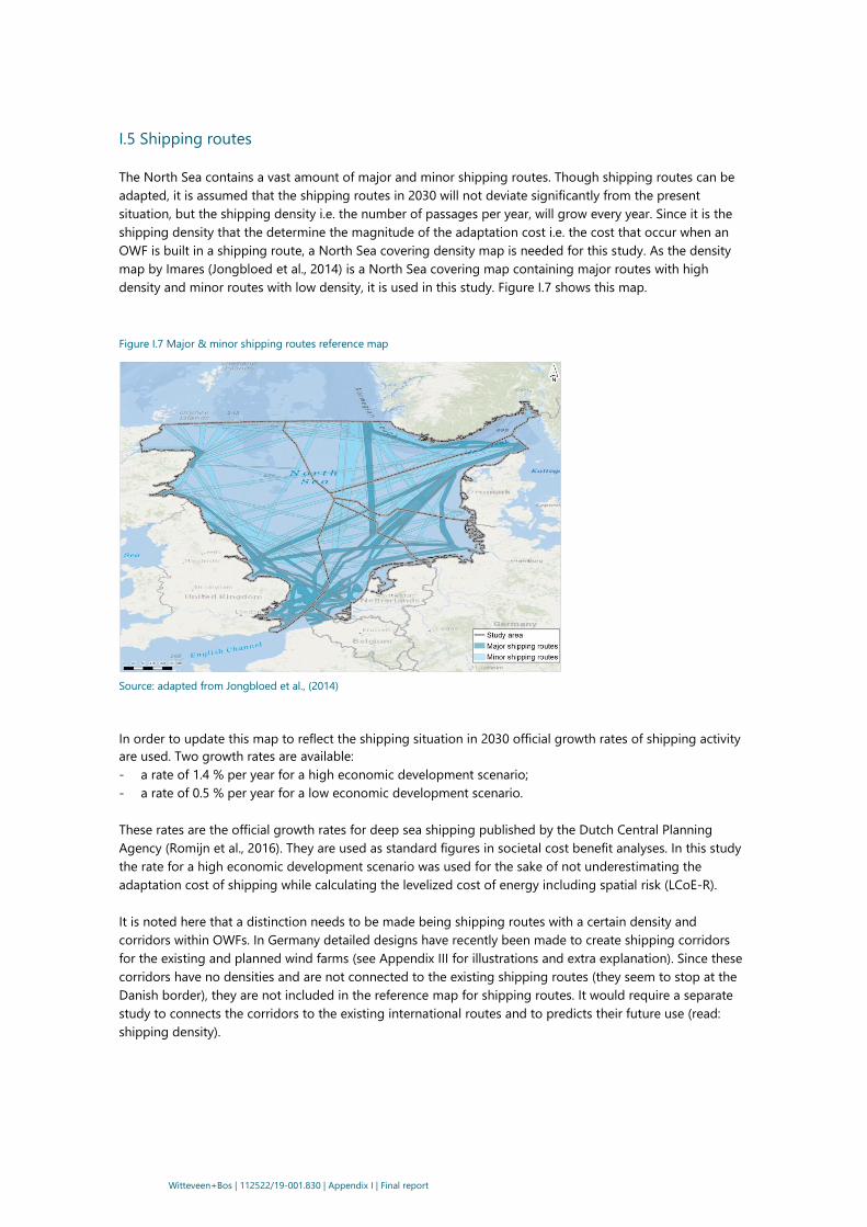
Witteveen+Bos | 112522/19-001.830 | Appendix I | Final report
I.5 Shipping routes
The North Sea contains a vast amount of major and minor shipping routes. Though shipping routes can be
adapted, it is assumed that the shipping routes in 2030 will not deviate significantly from the present
situation, but the shipping density i.e. the number of passages per year, will grow every year. Since it is the
shipping density that the determine the magnitude of the adaptation cost i.e. the cost that occur when an
OWF is built in a shipping route, a North Sea covering density map is needed for this study. As the density
map by Imares (Jongbloed et al., 2014) is a North Sea covering map containing major routes with high
density and minor routes with low density, it is used in this study. Figure I.7 shows this map.
Figure I.7 Major & minor shipping routes reference map
Source: adapted from Jongbloed et al., (2014)
In order to update this map to reflect the shipping situation in 2030 official growth rates of shipping activity
are used. Two growth rates are available:
- a rate of 1.4 % per year for a high economic development scenario;
- a rate of 0.5 % per year for a low economic development scenario.
These rates are the official growth rates for deep sea shipping published by the Dutch Central Planning
Agency (Romijn et al., 2016). They are used as standard figures in societal cost benefit analyses. In this study
the rate for a high economic development scenario was used for the sake of not underestimating the
adaptation cost of shipping while calculating the levelized cost of energy including spatial risk (LCoE-R).
It is noted here that a distinction needs to be made being shipping routes with a certain density and
corridors within OWFs. In Germany detailed designs have recently been made to create shipping corridors
for the existing and planned wind farms (see Appendix III for illustrations and extra explanation). Since these
corridors have no densities and are not connected to the existing shipping routes (they seem to stop at the
Danish border), they are not included in the reference map for shipping routes. It would require a separate
study to connects the corridors to the existing international routes and to predicts their future use (read:
shipping density).
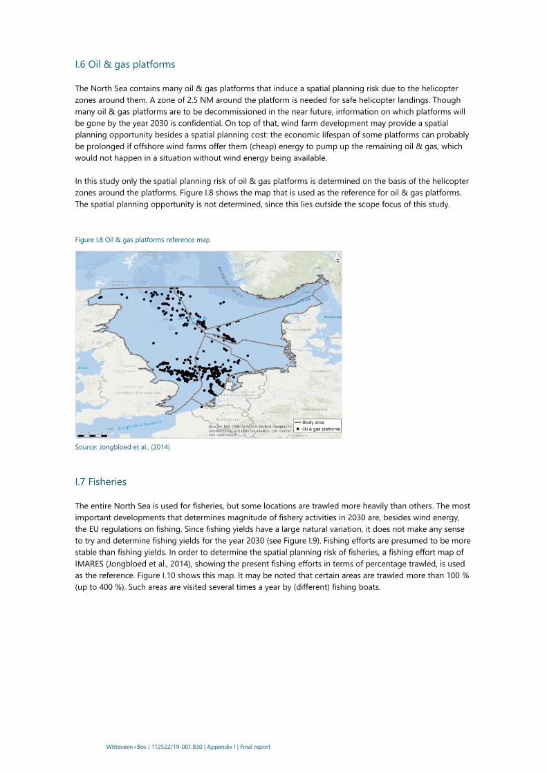
Witteveen+Bos | 112522/19-001.830 | Appendix I | Final report
I.6 Oil & gas platforms
The North Sea contains many oil & gas platforms that induce a spatial planning risk due to the helicopter
zones around them. A zone of 2.5 NM around the platform is needed for safe helicopter landings. Though
many oil & gas platforms are to be decommissioned in the near future, information on which platforms will
be gone by the year 2030 is confidential. On top of that, wind farm development may provide a spatial
planning opportunity besides a spatial planning cost: the economic lifespan of some platforms can probably
be prolonged if offshore wind farms offer them (cheap) energy to pump up the remaining oil & gas, which
would not happen in a situation without wind energy being available.
In this study only the spatial planning risk of oil & gas platforms is determined on the basis of the helicopter
zones around the platforms. Figure I.8 shows the map that is used as the reference for oil & gas platforms.
The spatial planning opportunity is not determined, since this lies outside the scope focus of this study.
Figure I.8 Oil & gas platforms reference map
Source: Jongbloed et al., (2014)
I.7 Fisheries
The entire North Sea is used for fisheries, but some locations are trawled more heavily than others. The most
important developments that determines magnitude of fishery activities in 2030 are, besides wind energy,
the EU regulations on fishing. Since fishing yields have a large natural variation, it does not make any sense
to try and determine fishing yields for the year 2030 (see Figure I.9). Fishing efforts are presumed to be more
stable than fishing yields. In order to determine the spatial planning risk of fisheries, a fishing effort map of
IMARES (Jongbloed et al., 2014), showing the present fishing efforts in terms of percentage trawled, is used
as the reference. Figure I.10 shows this map. It may be noted that certain areas are trawled more than 100 %
(up to 400 %). Such areas are visited several times a year by (different) fishing boats.
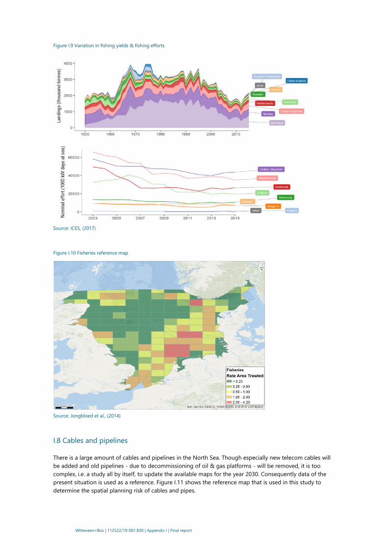
Witteveen+Bos | 112522/19-001.830 | Appendix I | Final report
Figure I.9 Variation in fishing yields & fishing efforts
Source: ICES, (2017)
Figure I.10 Fisheries reference map
Source: Jongbloed et al., (2014)
I.8 Cables and pipelines
There is a large amount of cables and pipelines in the North Sea. Though especially new telecom cables will
be added and old pipelines - due to decommissioning of oil & gas platforms - will be removed, it is too
complex, i.e. a study all by itself, to update the available maps for the year 2030. Consequently data of the
present situation is used as a reference. Figure I.11 shows the reference map that is used in this study to
determine the spatial planning risk of cables and pipes.

Witteveen+Bos | 112522/19-001.830 | Appendix I | Final report
Figure I.11 Cables and pipelines reference map
Source: Jongbloed et al., (2014)
It may be noted that cable costs are declining. As a result the interest for cable corridors that combine cables
is growing (Hoefsloot et al., 2018). This reduces the magnitude of spatial planning risk of cables and pipes.
I.9 Sand mining
The North Sea is an important source of sand that is used for coastal defence and as a building material. On
the one hand climate change increases the sand demand for coastal sand nourishments. On the other hand,
offshore wind energy may help to reduce climate change and thus reduces the sand demand for coastal
defence. The sand demand for building purposes depends on general economic developments. One would
expect it to grow over time. Since sand mining areas are appointed in order to cover the sand demand for
the next 100 years, maps with the presently appointed mining sites could serve as a reference. In this study
the mining site map of IMARES (Jongbloed et al., 2014) is used as reference. This map (see figure I.12)
includes both active and prospected sites. Sites to be closed soon are excluded from the map if the closure
date is known.
The actual sand mining activities are quite dynamic. Sand is taken whenever and where ever it is needed,
though the is key is to find sand as close as possible to its destination as transport cost are high. This is why
the spatial planning risk that sand mining generates is actually a so called option value: the value of mining
sites is to keep the option open to extract sand if needed.

Witteveen+Bos | 112522/19-001.830 | Appendix I | Final report
Figure I.12 Sand mining sites reference map
Source: Jongbloed et al., (2014)

Witteveen+Bos | 112522/19-001.830 | Appendix II | Final report
II
APPENDIX: SPATIAL COST CALCULATION FORMULAS
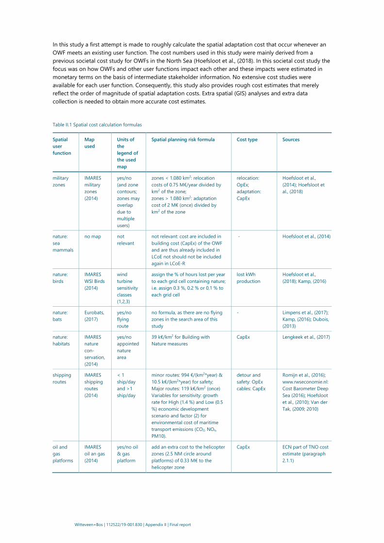
Witteveen+Bos | 112522/19-001.830 | Appendix II | Final report
In this study a first attempt is made to roughly calculate the spatial adaptation cost that occur whenever an
OWF meets an existing user function. The cost numbers used in this study were mainly derived from a
previous societal cost study for OWFs in the North Sea (Hoefsloot et al., (2018). In this societal cost study the
focus was on how OWFs and other user functions impact each other and these impacts were estimated in
monetary terms on the basis of intermediate stakeholder information. No extensive cost studies were
available for each user function. Consequently, this study also provides rough cost estimates that merely
reflect the order of magnitude of spatial adaptation costs. Extra spatial (GIS) analyses and extra data
collection is needed to obtain more accurate cost estimates.
Table II.1 Spatial cost calculation formulas
Spatial
user
function
Map
used
Units of
the
legend of
the used
map
Spatial planning risk formula Cost type Sources
military
zones
IMARES
military
zones
(2014)
yes/no
(and zone
contours;
zones may
overlap
due to
multiple
users)
zones < 1.080 km2: relocation
costs of 0.75 M€/year divided by
km2 of the zone;
zones > 1.080 km2: adaptation
cost of 2 M€ (once) divided by
km2 of the zone
relocation:
OpEx;
adaptation:
CapEx
Hoefsloot et al.,
(2014); Hoefsloot et
al., (2018)
nature:
sea
mammals
no map not
relevant
not relevant: cost are included in
building cost (CapEx) of the OWF
and are thus already included in
LCoE not should not be included
again in LCoE-R
- Hoefsloot et al., (2014)
nature:
birds
IMARES
WSI Birds
(2014)
wind
turbine
sensitivity
classes
(1,2,3)
assign the % of hours lost per year
to each grid cell containing nature;
i.e. assign 0.3 %, 0.2 % or 0.1 % to
each grid cell
lost kWh
production
Hoefsloot et al.,
(2018); Kamp, (2016)
nature:
bats
Eurobats,
(2017)
yes/no
flying
route
no formula, as there are no flying
zones in the search area of this
study
- Limpens et al., (2017);
Kamp, (2016); Dubois,
(2013)
nature:
habitats
IMARES
nature
con-
servation,
(2014)
yes/no
appointed
nature
area
39 k€/km2 for Building with
Nature measures
CapEx Lengkeek et al., (2017)
shipping
routes
IMARES
shipping
routes
(2014)
< 1
ship/day
and >1
ship/day
minor routes: 994 €/(km2*year) &
10.5 k€/(km2*year) for safety;
Major routes: 119 k€/km2 (once)
Variables for sensitivity: growth
rate for High (1.4 %) and Low (0.5
%) economic development
scenario and factor (2) for
environmental cost of maritime
transport emissions (CO2, NOx,
PM10).
detour and
safety: OpEx
cables: CapEx
Romijn et al., (2016);
www.rwseconomie.nl:
Cost Barometer Deep
Sea (2016); Hoefsloot
et al., (2010); Van der
Tak, (2009; 2010)
oil and
gas
platforms
IMARES
oil an gas
(2014)
yes/no oil
& gas
platform
add an extra cost to the helicopter
zones (2.5 NM circle around
platforms) of 0.33 M€ to the
helicopter zone
CapEx ECN part of TNO cost
estimate (paragraph
2.1.1)
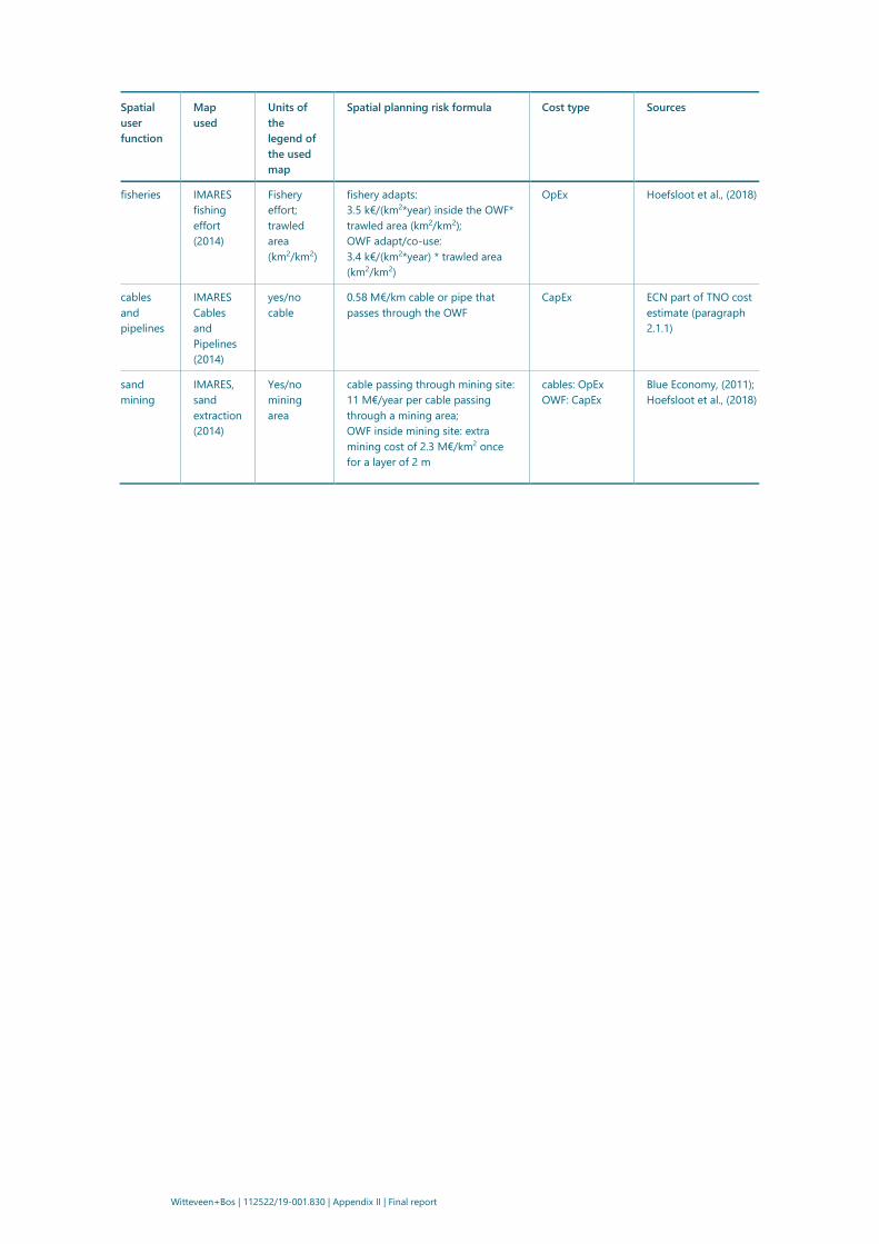
Witteveen+Bos | 112522/19-001.830 | Appendix II | Final report
Spatial
user
function
Map
used
Units of
the
legend of
the used
map
Spatial planning risk formula Cost type Sources
fisheries IMARES
fishing
effort
(2014)
Fishery
effort;
trawled
area
(km2/km2)
fishery adapts:
3.5 k€/(km2*year) inside the OWF*
trawled area (km2/km2);
OWF adapt/co-use:
3.4 k€/(km2*year) * trawled area
(km2/km2)
OpEx Hoefsloot et al., (2018)
cables
and
pipelines
IMARES
Cables
and
Pipelines
(2014)
yes/no
cable
0.58 M€/km cable or pipe that
passes through the OWF
CapEx ECN part of TNO cost
estimate (paragraph
2.1.1)
sand
mining
IMARES,
sand
extraction
(2014)
Yes/no
mining
area
cable passing through mining site:
11 M€/year per cable passing
through a mining area;
OWF inside mining site: extra
mining cost of 2.3 M€/km2 once
for a layer of 2 m
cables: OpEx
OWF: CapEx
Blue Economy, (2011);
Hoefsloot et al., (2018)

Witteveen+Bos | 112522/19-001.830 | Appendix III | Final report
III
APPENDIX: DETAILED DESIGN OF GERMAN SHIPPING CORRIDORS
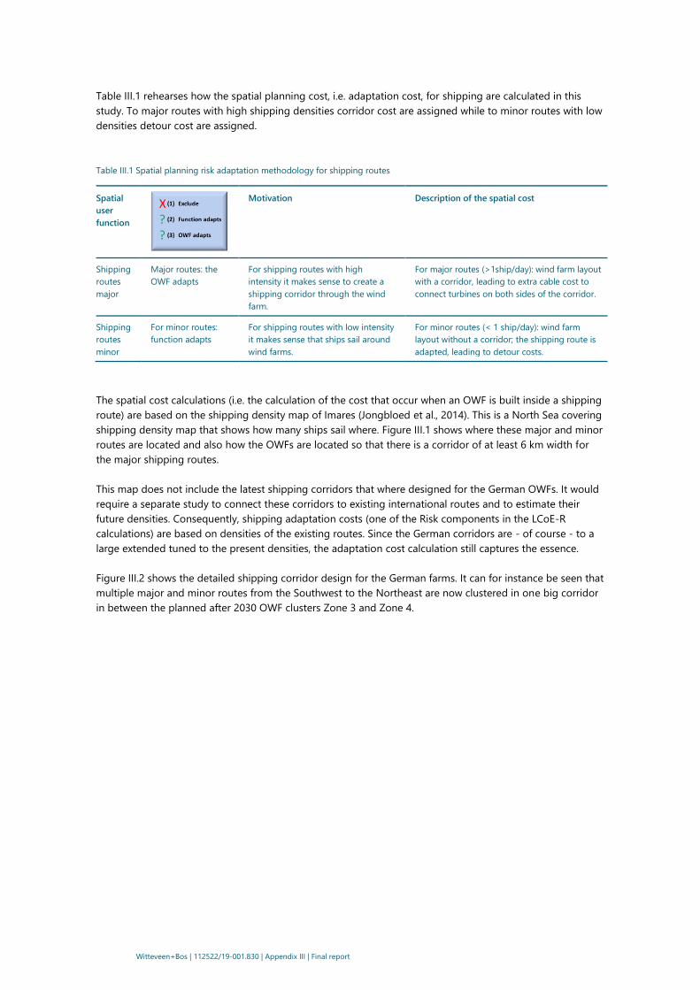
Witteveen+Bos | 112522/19-001.830 | Appendix III | Final report
Table III.1 rehearses how the spatial planning cost, i.e. adaptation cost, for shipping are calculated in this
study. To major routes with high shipping densities corridor cost are assigned while to minor routes with low
densities detour cost are assigned.
Table III.1 Spatial planning risk adaptation methodology for shipping routes
Spatial
user
function
Motivation Description of the spatial cost
Shipping
routes
major
Major routes: the
OWF adapts
For shipping routes with high
intensity it makes sense to create a
shipping corridor through the wind
farm.
For major routes (>1ship/day): wind farm layout
with a corridor, leading to extra cable cost to
connect turbines on both sides of the corridor.
Shipping
routes
minor
For minor routes:
function adapts
For shipping routes with low intensity
it makes sense that ships sail around
wind farms.
For minor routes (< 1 ship/day): wind farm
layout without a corridor; the shipping route is
adapted, leading to detour costs.
The spatial cost calculations (i.e. the calculation of the cost that occur when an OWF is built inside a shipping
route) are based on the shipping density map of Imares (Jongbloed et al., 2014). This is a North Sea covering
shipping density map that shows how many ships sail where. Figure III.1 shows where these major and minor
routes are located and also how the OWFs are located so that there is a corridor of at least 6 km width for
the major shipping routes.
This map does not include the latest shipping corridors that where designed for the German OWFs. It would
require a separate study to connect these corridors to existing international routes and to estimate their
future densities. Consequently, shipping adaptation costs (one of the Risk components in the LCoE-R
calculations) are based on densities of the existing routes. Since the German corridors are - of course - to a
large extended tuned to the present densities, the adaptation cost calculation still captures the essence.
Figure III.2 shows the detailed shipping corridor design for the German farms. It can for instance be seen that
multiple major and minor routes from the Southwest to the Northeast are now clustered in one big corridor
in between the planned after 2030 OWF clusters Zone 3 and Zone 4.

Witteveen+Bos | 112522/19-001.830 | Appendix III | Final report
Figure III.1 Major shipping routes with a corridor (left), minor shipping routes with detour costs (right)
Figure III.2 Shapefiles TenneT TSO GmbH, (2018) with blockages and alternative routes (left) & LCoE-R based set with possible new
locations excluding shipping (right)
Zone 4
Zone 3
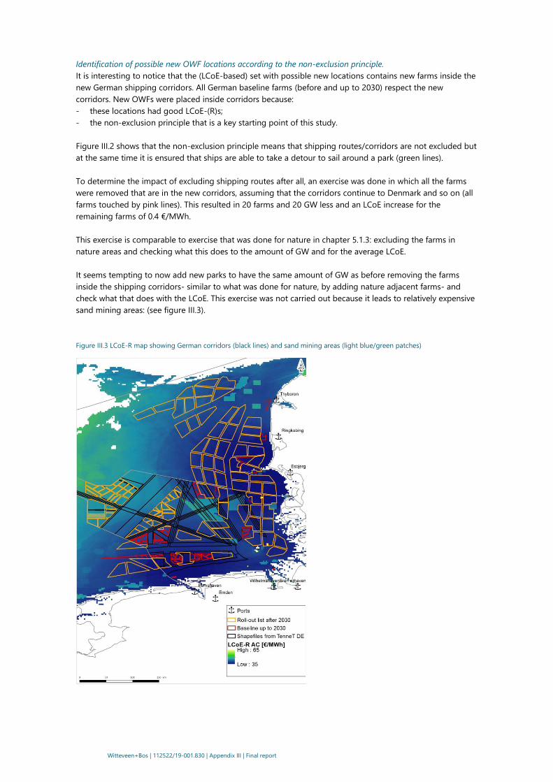
Witteveen+Bos | 112522/19-001.830 | Appendix III | Final report
Identification of possible new OWF locations according to the non-exclusion principle.
It is interesting to notice that the (LCoE-based) set with possible new locations contains new farms inside the
new German shipping corridors. All German baseline farms (before and up to 2030) respect the new
corridors. New OWFs were placed inside corridors because:
- these locations had good LCoE-(R)s;
- the non-exclusion principle that is a key starting point of this study.
Figure III.2 shows that the non-exclusion principle means that shipping routes/corridors are not excluded but
at the same time it is ensured that ships are able to take a detour to sail around a park (green lines).
To determine the impact of excluding shipping routes after all, an exercise was done in which all the farms
were removed that are in the new corridors, assuming that the corridors continue to Denmark and so on (all
farms touched by pink lines). This resulted in 20 farms and 20 GW less and an LCoE increase for the
remaining farms of 0.4 €/MWh.
This exercise is comparable to exercise that was done for nature in chapter 5.1.3: excluding the farms in
nature areas and checking what this does to the amount of GW and for the average LCoE.
It seems tempting to now add new parks to have the same amount of GW as before removing the farms
inside the shipping corridors- similar to what was done for nature, by adding nature adjacent farms- and
check what that does with the LCoE. This exercise was not carried out because it leads to relatively expensive
sand mining areas: (see figure III.3).
Figure III.3 LCoE-R map showing German corridors (black lines) and sand mining areas (light blue/green patches)

www.witteveenbos.com