Cost efficiency analysis of electricity distribution networks: Application of the StoNED method in the Finnish regulatory model

Timo Kuosmanen

School of Economics, Aalto University, 00100 Helsinki, Finland

E-mail. timo.kuosmanen@aalto.fi

Abstract

Electricity distribution network is a prime example of a natural local monopoly. In many countries,

electricity distribution firms are regulated by the government. In Finland, the regulator estimates the

efficient cost frontier using the data envelopment analysis (DEA) and stochastic frontier analysis (SFA)

methods. This paper reports the main results of the research project commissioned by the Finnish

regulator for further development of the efficiency estimation in their regulatory model. The key

objectives of the project were to integrate a stochastic SFA-style noise term to the nonparametric,

axiomatic DEA-style cost frontier, and take into account the heterogeneity of firms and their operating

environments. To estimate the resulting stochastic semi-parametric cost frontier model, a new method

called stochastic nonparametric envelopment of data (StoNED) is proposed. Based on the insights

obtained in the empirical analysis using real data of the regulated networks, replacing the currently used

DEA and SFA methods by the StoNED method is recommended.

Key words:

Energy markets; heterogeneity; nonparametric production analysis; productive efficiency

2

1. Introduction

Distribution of electricity to end users forms the final stage of the supply network of electricity. The

distribution networks usually take power from high voltage transmission lines and distribute it to electricity

consuming firms and households. Since construction of competing networks in the same area is usually

prohibitively expensive, the distribution networks enjoy a natural monopoly within their established

distribution area. In many countries, the national or local governments have established regulatory agencies

to monitor the electricity distribution networks and counter the abuse of local monopoly power. Thus, the

immediate challenge faced by the regulators is to determine an acceptable price for electricity distribution in

a sector characterized a heterogeneous group of firms operating in heterogeneous environments. In the long

run, a related challenge is to provide incentives for improving productivity and adopting the best

technologies and practices.

The regulation of electricity distribution networks typically involves both static and dynamic cost

efficiency analysis of the distribution firms. This is one of the most significant application areas of the

productive efficiency analysis in terms of the policy relevance and economic implications. The frontier

estimation techniques such as data envelopment analysis (DEA; Farrell 1975; Charnes et al., 1978) and

stochastic frontier analysis (SFA; Aigner et al., 1977; Meeusen and vanden Broeck, 1977) are widely

employed by regulatory agencies around the world. Some of the recent published applications include

Pahwa et al. (2003) [USA], Jamasb and Pollit (2003) [Europe], Edvardsen and Forsund (2003) [Nordic

countries], Estache et al. (2004) [South America], Filippini et al. (2004) [Slovenia], Thakur et al. (2005)

[India], von Hirschhausen et al. (2006) [Germany], Cullmann and von Hirschhausen (2008) [Poland], and

Kopsakangas-Savolainen and Svento (2008) [Finland].

Nordic countries have a particularly strong tradition in the applications of the frontier estimation

techniques to the regulation of electricity distribution (Hjalmarsson and Veiderpass, 1992; Forsund and

Kittelsen, 1998; Agrell et al., 2005). In Finland, the Energy Market Authority (Energiamarkkinavirasto,

henceforth referred to as EMV) has applied the DEA method since 1998. The landmark study by

Korhonen, Syrjänen and Tötterström (2000) [a shorter version published in English in Korhonen and

Syrjänen, 2003], defined the input and output variables and the main axioms of the DEA-based cost frontier

3

that are still applied by EMV in its current regulatory model. Another significant development in the

evolution of the Finnish model was the study by Syrjänen, Bogetoft and Agrell (2006), which recommended

the adoption of SFA as a parallel frontier estimation technique in addition to DEA. In years 2008-2011 the

regulatory model of EMV sets the efficiency improvement targets based on the arithmetic average of the

firm-specific DEA and SFA efficiency estimates. The purpose of using the average efficiency estimate is to

reduce the statistical uncertainty related to both DEA and SFA methods and their underlying assumptions.

As a logical next step in the evolution of the Finnish regulatory model, EMV commissioned a

research project to investigate how the essential characteristics of the DEA and SFA methods could be

integrated in the Finnish regulatory model by employing a unified stochastic frontier method called

StoNED (stochastic nonparametric envelopment of data), developed in Kuosmanen (2006, 2008) and Kuosmanen

and Kortelainen (2007). The StoNED method combines the non-parametric, piece-wise linear DEA-style

frontier with the stochastic SFA-style treatment of inefficiency and noise. The assumptions of the StoNED

method are milder than those required by DEA or SFA: both DEA and SFA can be obtained as

constrained special cases of the more general StoNED-model (Kuosmanen and Johnson, 2010). This makes

the StoNED method more robust to the statistical uncertainty concerning the exact functional form of the

cost frontier and the impacts of stochastic noise than the classic DEA and SFA methods.

This paper reports the main results of the project (the final report by Kuosmanen et al. 2010

contains additional material but it is only available in Finnish). We believe the findings of this study are very

interesting both for the research community in the field of productive efficiency analysis and for the

regulatory agencies in other countries. This study demonstrates the practical benefits of the StoNED

method over the classic DEA and SFA approaches in a real world regulatory application. While this study

focuses on the electricity distribution networks, the novel analytical techniques employed in this study are

broadly applicable to the regulation of natural monopolies and networks not only in energy sector but in

other industries as well.

The rest of the paper is organized as follows. Section 2 introduces the cost frontier model and its

maintained assumptions. Section 3 presents the StoNED method for estimating the functions and

parameters of interest. Section 4 briefly describes the data. In Section 5 we present the main empirical

4

results based on our preferred model specification. In Section 6 we report some specification tests and

sensitivity analyses based on alternative model specifications and assumptions. Section 7 presents the

concluding remarks and the policy recommendations. Additional 3-D graphical illustrations of the

StoNED-frontier are provided in the Appendix.

2. Cost frontier model

The cost frontier model employed by EMV uses the total cost as the single aggregate input factor. The

total cost of firm i is denoted by xi, and it includes the total capital expenditure, controllable operational

expenditure, and the cost of interruptions. The three output variables (y) specified in the model are: y1

is the weighted amount of energy transmitted through the network (GWh of 0.4 kV equivalents), y2 is

the total length of the network (km), and y3 is the total number of customers connected to the network.

In output y1, the transmission of electricity at different voltage levels is weighted according to the

average cost of transmission such that the high-voltage transmission gets a lower weight than the low-

voltage transmission. The specification of the input and output variables is based on EMV’s current

regulatory model and it is commonly used in the literature (see e.g. Korhonen and Syrjanen, 2003;

Thakur et al., 2007).

In addition to the outputs y, the proportion of underground cables in the total length of the

network is taken into account as a contextual variable z. The rationale of using an additional z variable

that is not an input or output as such is to better control for the heterogeneity of the firms and their

operating environments. In Finland, underground cables are widely used in the cities and suburban

areas, but the overhead power-lines remain a more economical technology in the rural and sparsely

populated areas. By using the proportion of underground cables as a contextual variable we take into

account the higher cost of underground cables, but this is not the only purpose of this variable. More

importantly, we are also trying to capture a range of other effects of urban versus rural operating

environment on firm performance. For example, the average wage rate is generally higher in large cities

and towns than in rural areas where the employment opportunities are scarce and thus the opportunity

5

cost of labor is lower. Thus, the contextual variable z is likely capture the statistical effect of higher

wage rate on total cost, among many other sources of heterogeneity.

The cost frontier model considered in this study can be analytically presented as

( ) exp( )i i i i ix C z u vy ,

where C is the frontier cost function, is a parameter that characterizes the effect of underground

cables z on firm’s total cost, ui is a random variable that represents cost inefficiency of firm i, and vi is a

stochastic noise term that captures the effects of measurement errors, omitted variables and other

random disturbances to the otherwise stable cost equation.

We do not assume any specific functional form for the cost function C. Similar to the classic

DEA (Charnes et al., 1978), we impose the following axioms:

1) C is monotonic increasing in all outputs y (the sub-gradients satisfy ( ) C y 0 y ).

2) C is globally convex ( 31 2 1 2 1 2( (1 ) ) ( ) ((1 ) ) 0; ,C C Cy y y y y y ).

3) C exhibits constant returns to scale (CRS) ( ( ) ( ) 0C Cy y ).

The random variables u and v are assumed to independently distributed of each other, and of outputs y

and contextual variable z. Following the classic SFA studies (Aigner et al. 1977), the noise term v is

assumed to be normally distributed with a zero mean a finite variance 2 0v and the inefficiency term

u follows the half-normal distribution with a finite variance 2 0u . The expected value of inefficiency

is denoted by ( )iE u , and it is known to be directly proportional to the parameter u :

2 /u (Aigner et al. 1977).

This model is more general in its assumptions than the classic DEA and SFA models currently

employed by EMV. It is easy to verify that the original DEA specification by Charnes et al. (1978) is

obtained as the restricted special case of the above model if we set 2 0v (no noise) and = 0

(exclude the contextual variable). Similarly, the linear SFA model proposed by Syrjänen et al. (2006) is

obtained by imposing the additional parametric assumption that cost frontier C is a linear function.

6

Thus, both DEA and SFA specifications are restricted special cases of the more general model assumed

in this paper.

EMV currently sets the efficiency improvement targets based on the arithmetic average of the

DEA and SFA efficiency estimates. The main purpose of this procedure is to reduce the statistical

uncertainty related to both DEA and SFA estimators and their underlying assumptions. However, the

statistical properties of the two estimators are only known under the very restrictive conditions where

the assumptions of both DEA and SFA hold simultaneously (i.e., the cost function is linear and there is

no noise). Under these assumptions the SFA estimator is unbiased, consistent, and asymptotically

efficient, whereas the DEA estimator is consistent but biased. In the ideal case, the SFA estimator is

more efficient than the arithmetic average of DEA and SFA. Unfortunately, neither DEA nor SFA are

very robust to the violation of their basic assumption. There is no evidence that averaging the DEA

and SFA estimators improve the precision of the estimator if the assumptions of either one of the

methods - or both – fail to hold. A method that builds upon a more general set of assumptions is the

logical way forward.

3. StoNED method

In this section we present the StoNED method (stochastic nonparametric envelopment of data) for estimating

the general cost frontier model introduced in the previous section. In contrast to the classic DEA and

SFA approaches, the StoNED method does not require any additional assumptions or parameter

restrictions. The StoNED method has two steps:

1) estimation of the expected total costs and the parameter by nonparametric least squares

2) estimation of the expected inefficiency, variance parameters, and firm-specific inefficiencies

First, without loss of generality, we can introduce a composite error term i i iu v , and

linearize the cost frontier model by taking natural logarithms of both sides of the equation to obtain

ln ln ( )i i i ix C zy .

7

This gives a semiparametric, partial linear model to be estimated. Convex nonparametric least squares

(CNLS: Kuosmanen, 2008; Johnson and Kuosmanen, 2009) regression provides consistent estimator

for the expected value of the total cost xi and the parameter . The CNLS estimator is obtained as the

optimal solution to the following least squares problem, which can be solved by convex programming

algorithms and solvers

2

, , , 1

min

. .ln ln

,

n

ii

i i i i

i i i

i h i

i

s tx z i

ih i

i

yy

0

Coefficients i can be interpreted as marginal costs of outputs or as the coefficients of the tangent

hyperplanes to the piece-wise linear cost frontier. These coefficients are analogous to the multiplier

weights in DEA. In contrast to the linear regression model, the coefficients i are specific to each firm.

This is an important feature for modeling heterogeneity of the distribution networks: urban distribution

networks with a large number of customers are generally assigned a higher marginal cost for output y3

than the rural networks, for which the length of the network (output y2) is a more important cost driver.

Parameter i is the CNLS estimator of the expected total cost of producing yi, that is, E(xi) =

C(yi) + µ. To estimate the cost frontier, we need to estimate µ that remains unknown after the first

step. To this end, we can utilize the distribution of the CNLS residuals ˆi , obtained in the optimal

solution to the CNLS problem (see Kuosmanen and Kortelainen, 2007, for details). Under the

maintained assumptions of half-normal inefficiency and normal noise, the second and third central

moments of the composite error distribution are given by

2 22

2u vM , 3

32 4

1 uM .

These central moments can be estimated by using the CNLS residuals:

8

22

1

ˆ ˆ( ) /n

ii

M n , 33

1

ˆ ˆ( ) /n

ii

M n .

Note that the third moment M3 (which measures the skewness of the distribution) only depends on the

standard deviation parameter u of the inefficiency distribution. Thus, given the estimated 3M̂ (which

should be positive in the case of a cost frontier), we can estimate u parameter by

3

3

ˆˆ

2 4 1u

M .

Subsequently, the standard deviation of the error term v is estimated using

22

2ˆˆ ˆv uM .

These MM estimators are unbiased and consistent (Aigner et al., 1977; Greene, 2008).

The cost function C is estimated by

ˆ ( )StoNEDC y = ˆexp( 2 / )i u .

Since both i and ˆu are statistically consistent, the estimator ˆ ( )StoNEDC y is also consistent. In practice,

the StoNED cost frontier is obtained by shifting the CNLS estimate of the average-practice production

function upwards by the expected value of the inefficiency term, analogous to the MOLS approach

(e.g., Greene, 2008).

Firm-specific inefficiency components ui must be inferred indirectly in the cross-sectional

setting. Jondrow et al. (1982) have shown that the conditional distribution of inefficiency ui given i is a

zero-truncated normal distribution with mean 2 2 2/( )i u u v and variance

2 2 2 2 2/ ( )u v u v . As a point estimator of ui, one can use the conditional mean

( / )( )1 ( / )i iE u ,

where is the standard normal density function, and is the standard normal cumulative

distribution function (see Kuosmanen and Kortelainen, 2007, for details). The conditional expected

9

value is an unbiased but inconsistent estimator of ui: irrespective of the sample size n, we have only a

single observation of the firm i (see, e.g., Greene, 2008, Section 2.8.2, for further discussion). The

Jondrow et al. (1982) estimates ˆ iu can be converted to cost efficiency measures (CE) expressed in the

percentage scale by using

ˆ 100% exp( )iCE u .

The range of the cost efficiency scores CE is [0%, 100%], where CE=100% corresponds to cost

efficient activity level.

Finally, Johnson and Kuosmanen (2009) show that the CNLS estimator of the parameter is

unbiased, consistent, asymptotically normal and efficient, and converges at the standard parametric rate

of order n-1/2. Thus, the essential statistical properties of the parametric estimators carry over to the

parametric part of the semiparametric estimator, even though the cost frontier C is estimated in a fully

nonparametric fashion. This enables us to apply conventional methods of inferences for testing the

statistical significance of the contextual variable z.

4. Data

The total cost x, the three input variables y, and the contextual variable z were introduced in Section 2.

As the regulatory model is based on four-year periods, EMV applies the average total cost and the

average output levels in the previous four-year period as the input-output variables of the cross-

sectional cost frontier model. In the similar fashion, the empirical data used in this study consists of

four-year averages over the period 2005-2008. Prior to averaging, all cost variables have been deflated

to the price level of 2005 using the price index of the construction sector published by the Statistics

Finland.

Table 1 reports descriptive statistics of the observed x, y and z variables. The total cost of the

sector was approximately 750 Million € per year during the study period (at the prices of year 2005).

The average total cost was approximately 8.5 Million €, but the maximum was as high as 117.5 Million

€. The total cost of the two largest distributors (Fortum Sähkönsiirto Oy and Vattenfall Verkko Oy)

10

forms approximately 30% of the total cost of the sector, while a large majority of the companies are

small local operators. This shows as relatively large skewness in all variables reported in Table 1.

Table 1: descriptive statistics of the input, output, and contextual variables (four-year averages of period 2005-2008). Variable Mean St. Dev. Kurtosis Skewness Min. Max. x = Total cost (1,000 €) 8,418.91 18,047.78 25.04 4.75 267.81 117,554.10 y1 =Energy transmission (GWh) 480.39 971.51 22.41 4.41 14.81 6,599.71 y2 =Length of network (km) 4,135.27 10,223.27 26.88 4.99 50.80 67,611.05 y3 =No. customers 35,448.68 71,870.65 17.08 3.98 24.25 420,473.00 z = Proportion of underground cables in the total network length 0.33 0.26 -0.52 0.73 0.01 1.00

The amount of energy transmission y1 measures the direct (variable) output of the distribution

activity. In contrast, outputs y2 and y3 represent the potential output or the capacity. It is worth to note

that distribution of electricity to recreational homes forms a significant proportion of activity for the

companies located in rural areas. Recreational homes consume relatively small amount of electricity,

especially in winter months when recreational homes are not used. However, the network companies

have a legal obligation to connect all customers within their designated area, and the firms have to

maintain the power lines in operation even if they are only used seasonally, which can be relatively

costly. To take this into account, outputs y2 and y3 capture the fixed cost of maintaining a sufficient

capacity to serve their designated network area irrespective of the actual consumption of power.

Several earlier studies have used the peak load (e.g., the maximum transmission of energy

within a period of one hour) or the load factor (i.e., the ratio of peak load to average load) as output

variables that measure the network capacity (e.g., Kopsakangas-Savolainen and Svento, 2008).

However, in the present data set the peak load correlates almost perfectly with the output variable y1:

the correlation coefficient of the peak load and the average load is r = 0.996. Therefore, introducing the

peak load as an output variable would cause serious multicollinearity problems for the estimation.

Further, introducing additional output variables affects the precision of the semi- and non-parametric

estimators due to the curse of dimensionality. The present set of output variables effectively captures

11

the costs associated with the peak load through the high statistical correlation with the output variable

y1 even though the peak load is not explicitly included in the model.

To some extent, the three output variables can take into account heterogeneity of firms and

their operating environments. In general, networks located in rural areas have a long network (y2)

relative to the number of customers (y3), whereas urban networks have a relatively short network. Thus,

the ratio y3 / y2 captures reasonably well the heterogeneity of urban versus rural networks. Note that in

the StoNED method the marginal costs of outputs can differ across firms, so the performance of rural

networks can be best rationalized by assigning a relatively large marginal cost for the network length

and a small marginal cost for the number of customers. In contrast, urban networks are evaluated in

the most favorable light by assigning large marginal cost on the number of customers and a small

marginal cost on the network length. The logic of assigning the marginal costs follows directly

analogous to the shadow pricing approach of the classic DEA.

While the output variables y2 and y3 can draw a distinction between urban versus rural

networks, the networks located in large cities have very similar output structure as those located in

suburbs or small towns. To better capture the differences in the output structures and operating

environments of the urban versus suburban networks, we have introduced the proportion of

underground cables as a z variable that represents the net impact of practices and operational

conditions on the total cost. In this study the proportion of underground cables is calculated based on

the total network length. Alternative z variables as well as alternative definitions of the proportion of

underground cables (e.g., the proportion of underground cables in the medium-voltage network) were

considered. The model specification reported in this paper was chosen based on the empirical fit of the

model (R2), taken into account the economic and statistical significance of the z variables considered.

Note that some earlier studies have similarly used the proportion of underground cables as an

explanatory variable in the second-stage regression where DEA efficiency scores are regressed on z

variables. In contrast to those studies, the coefficient of the z variable is here jointly estimated together

with the nonparametric cost frontier. This integrated estimation procedure allows us to avoid the

12

omitted variable bias of the efficiency estimation (if z variable is ignored in the first stage efficiency

analysis), and the standard techniques of statistical inferences are applicable (see Johnson and

Kuosmanen, 2009, for details).

5. Results

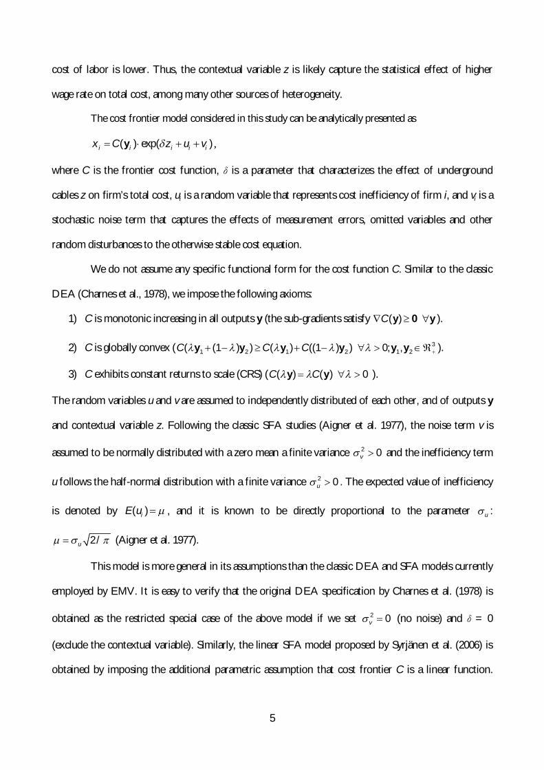
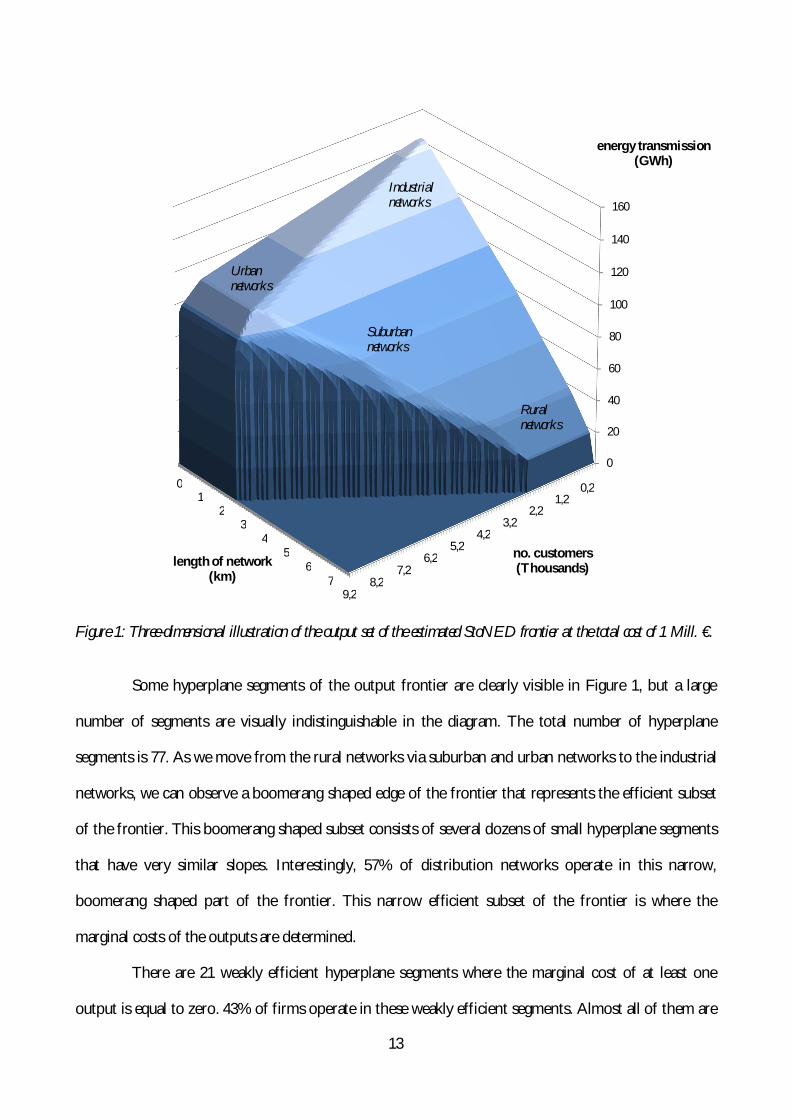
The estimated StoNED-frontier is graphically illustrated in Figure 1. The three-dimensional diagram

displays the output set at the fixed cost level of one Million €. The three axes of the diagram represent

the three output variables: energy transmission, length of network, and number of customers. The

piece-wise linear boundary presented in Figure 1 describes the output combinations that can be

produced with the total expenditure of one Million €. Of course, output combinations below the

efficient frontier are also feasible according to the free disposability assumption. The origin of the

output set lies below the frontier: Figure 1 displays the estimated output frontier from outside.

To gain intuition, we have indicated the approximate locations of rural, suburban, urban, and

industrial networks in Figure 1. Rural networks have relatively large length of the network, but low

energy transmission and small number of customers. These networks are located in the bottom right

corner of Figure 1. When we move towards suburban and urban networks, the number of customers

and energy transmission increase while the length of network decreases. Networks operating in large

cities are found in the top left corner of Figure 1. The data set also includes a small number of

industrial networks that supply energy to a small number of large manufacturing plants. These

industrial networks have a relatively large amount of energy transmission, whereas the length of

network and the number of customers can be very small. The industrial networks are found on the top

of the diagram. In some industrial towns the heavy industry can consume a large proportion of energy

distributed through the network. The output profiles of the networks located in industrial towns are

somewhere between the large cities (left corner) and the industrial networks (top corner) in the figure.

13

Figure 1: Three-dimensional illustration of the output set of the estimated StoNED frontier at the total cost of 1 Mill. €.

Some hyperplane segments of the output frontier are clearly visible in Figure 1, but a large

number of segments are visually indistinguishable in the diagram. The total number of hyperplane

segments is 77. As we move from the rural networks via suburban and urban networks to the industrial

networks, we can observe a boomerang shaped edge of the frontier that represents the efficient subset

of the frontier. This boomerang shaped subset consists of several dozens of small hyperplane segments

that have very similar slopes. Interestingly, 57% of distribution networks operate in this narrow,

boomerang shaped part of the frontier. This narrow efficient subset of the frontier is where the

marginal costs of the outputs are determined.

There are 21 weakly efficient hyperplane segments where the marginal cost of at least one

output is equal to zero. 43% of firms operate in these weakly efficient segments. Almost all of them are

9,28,2

7,26,2

5,24,2

3,22,2

1,20,2

0

20

40

60

80

100

120

140

160

01

23

45

67

no. customers(Thousands)

energy transmission(GWh)

length of network(km)

Industrial networks

Urban networks

Ruralnetworks

Suburbannetworks

14

located in the large weakly efficient triangle on the right side of the diagram where the marginal cost of

the number of customers is equal to zero. These firms are typically small networks operating in the

rural areas, with a relatively small number of customers. Only one network operates in the smaller

weakly efficient subset where the marginal cost of the network length is zero (on the left side of the

diagram). None of the distribution firms operate in the dark colored vertical part of the frontier where

the marginal cost of electricity transmission is equal to zero.

As the StoNED method is based on least squares regression, the empirical fit of the model

can be measured by using the conventional coefficient of determination (R2). As the model has been

specified in the log-linear form, the coefficient of determination measures the proportion of the

variance of natural logarithm of total costs (ln x) explained by the model. The statistic is defined as

2 ˆ. ( )1. (ln )

Est VarREst Var x

where

ˆ. ( )Est Var is the sample variance of the CNLS residuals,

. (ln )Est Var x is the sample variance of the total cost x.

The coefficient of determination obtained by the previous formula is 0.9864. This means that

the StoNED cost frontier explains over 98 percent of the observed variation in the natural logarithm of

total cost across the networks. The R2 statistic includes the effects of three outputs y1, y2, y3, the

contextual variable z, and the expected value of the inefficiency term u The 1.36% of variation that

remains unexplained by the model includes the deviations of the inefficiency term u from its mean, and

the noise term v. By construction, the StoNED frontier maximizes the empirical fit under the

postulated axioms: no other cost function C that satisfies free disposability, convexity and constant

returns to scale can achieve a higher R2 statistic.

As the cost function is assumed to exhibit constant returns to scale, the shape of the output

sets remains the same at all non-negative cost levels. That is, the diagram presented in Figure 1 applies

15

to different cost levels if we simply rescale the axes. For example, at the total cost of 10 Mill. €, the

numbers on the three axes should be multiplied by factor 10, but otherwise the same diagram applies.

Figure 1 reveals the complexity of the estimation problem. If we estimate the cost function by

the linear SFA model (currently applied by EMV), the results will be driven by the large weakly efficient

triangle on the right of the diagram. However, the relevant marginal costs of outputs are determined on

the boomerang shaped efficient set of Figure 1. Clearly, the cost structure of rural networks is very

different from those of the urban or industrial networks. The linear SFA model applies the same

marginal costs to all distribution networks, whereas the StoNED model takes into account the

heterogeneity of the firms and their cost structures into account by allowing the marginal costs differ

across firms depending on their output structure. To assess all networks in the most favorable light, the

StoNED method assigns urban networks a relatively large marginal cost to the number of customers,

whereas the rural networks are assigned a relatively large marginal cost to the length of network.

Table 2 reports some descriptive statistics of the distribution of the estimated marginal costs.

These marginal costs are obtained by multiplying the shadow prices obtained as the optimal solution

to the CNLS problem by the expected value of inefficiency µ. Although the shadow prices are firm-

specific, in practice, the shadow prices tend to be heavily clustered. For 33 networks the shadow prices

are close to the median values reported in Table 2. On the other hand, it is worth to note that the

shadow prices are not necessarily unique (analogous to DEA). From Figure 1 it is evident that for the

firms located in the vertices or edges of the piecewise linear frontier it is impossible to determine any

unique tangent hyperplane. There are as many as 39 such firms in our sample. For these firms we have

estimated the marginal costs as the arithmetic average of all adjacent efficient and weakly efficient

hyperplane segments.

It is interesting to compare the results of Table 2 with the marginal cost estimates obtained by

linear regression. The OLS estimates of the marginal costs are 0.28 c/GWh for energy transmission,

895 €/km for the length of network, and 95 €/user for the number of customers. These estimates are

of similar magnitude as the firm-specific StoNED estimates reported in Table 2. However, according to

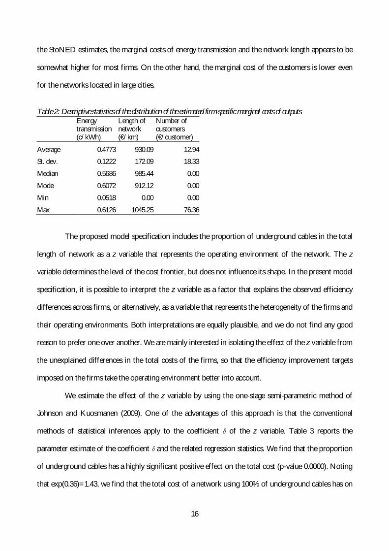
16

the StoNED estimates, the marginal costs of energy transmission and the network length appears to be

somewhat higher for most firms. On the other hand, the marginal cost of the customers is lower even

for the networks located in large cities.

Table 2: Descriptive statistics of the distribution of the estimated firm-specific marginal costs of outputs

Energy transmission (c/kWh)

Length of network (€/km)

Number of customers (€/customer)

Average 0.4773 930.09 12.94 St. dev. 0.1222 172.09 18.33 Median 0.5686 985.44 0.00 Mode 0.6072 912.12 0.00 Min 0.0518 0.00 0.00 Max 0.6126 1045.25 76.36

The proposed model specification includes the proportion of underground cables in the total

length of network as a z variable that represents the operating environment of the network. The z

variable determines the level of the cost frontier, but does not influence its shape. In the present model

specification, it is possible to interpret the z variable as a factor that explains the observed efficiency

differences across firms, or alternatively, as a variable that represents the heterogeneity of the firms and

their operating environments. Both interpretations are equally plausible, and we do not find any good

reason to prefer one over another. We are mainly interested in isolating the effect of the z variable from

the unexplained differences in the total costs of the firms, so that the efficiency improvement targets

imposed on the firms take the operating environment better into account.

We estimate the effect of the z variable by using the one-stage semi-parametric method of

Johnson and Kuosmanen (2009). One of the advantages of this approach is that the conventional

methods of statistical inferences apply to the coefficient of the z variable. Table 3 reports the

parameter estimate of the coefficient and the related regression statistics. We find that the proportion

of underground cables has a highly significant positive effect on the total cost (p-value 0.0000). Noting

that exp(0.36)=1.43, we find that the total cost of a network using 100% of underground cables has on

17

average 43% higher total cost than an identical network using overhead cables. The z variable explains

approximately 30% of the differences in the logarithm of cost efficiency [lnTOTEXi – lnC(yi)] across

networks (the partial R2 statistic reported on the bottom row of Table 3). It is worth emphasizing that

the z variable does not only capture the direct cost of using underground cables, but also other factors

correlated with the z variable. Since underground cables are mainly used in urban and suburban areas,

the statistical correlation between the total cost and the z variable will also capture such effects as the

higher wage rate in the cities, which has nothing to do with the physical construction or maintenance of

the distribution network. We interpret the z variable as a proxy for the urban operating environment. It

is difficult to find exact measures of the operating environment, but we find that a large proportion of

otherwise unexplained cost differences across firms can be explained by the differences in the

utilization of underground cables.

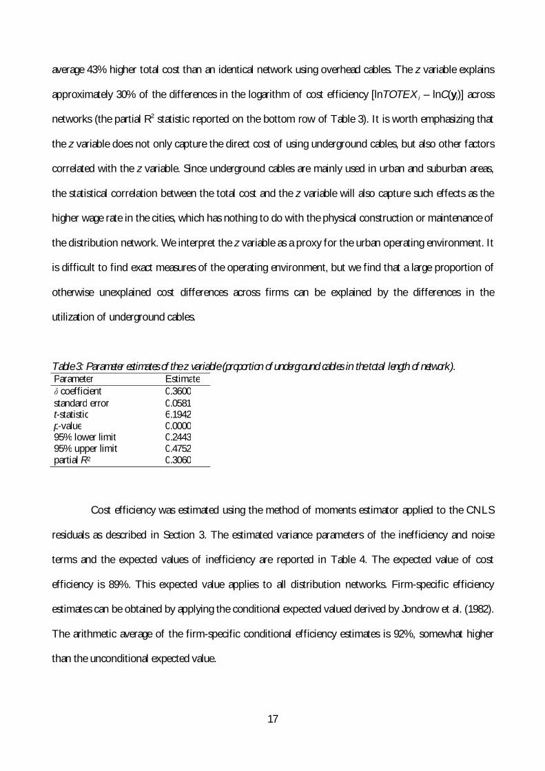
Table 3: Parameter estimates of the z variable (proportion of underground cables in the total length of network). Parameter Estimate coefficient 0.3600

standard error 0.0581 t-statistic 6.1942 p-value 0.0000 95% lower limit 0.2443 95% upper limit 0.4752 partial R2 0.3060

Cost efficiency was estimated using the method of moments estimator applied to the CNLS

residuals as described in Section 3. The estimated variance parameters of the inefficiency and noise

terms and the expected values of inefficiency are reported in Table 4. The expected value of cost

efficiency is 89%. This expected value applies to all distribution networks. Firm-specific efficiency

estimates can be obtained by applying the conditional expected valued derived by Jondrow et al. (1982).

The arithmetic average of the firm-specific conditional efficiency estimates is 92%, somewhat higher

than the unconditional expected value.

18

Table 4: Parameter estimates related to the inefficiency and the noise terms and the expected value of inefficiency Parameter Estimate

2 (variance of the composite error term) 0.03239 2u (variance of the inefficiency term) 0.02064

2v (variance of the noise term) 0.01175

µ (expected value of the inefficiency term) 0.11464 Expected value of cost efficiency 89%

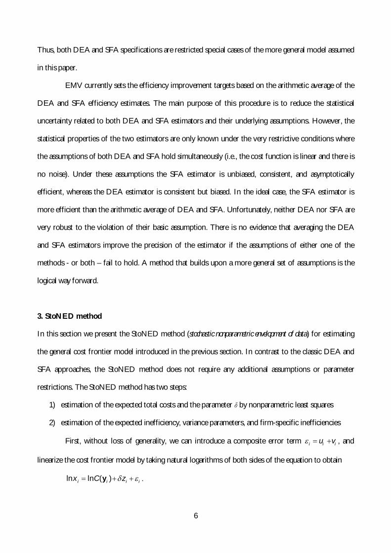
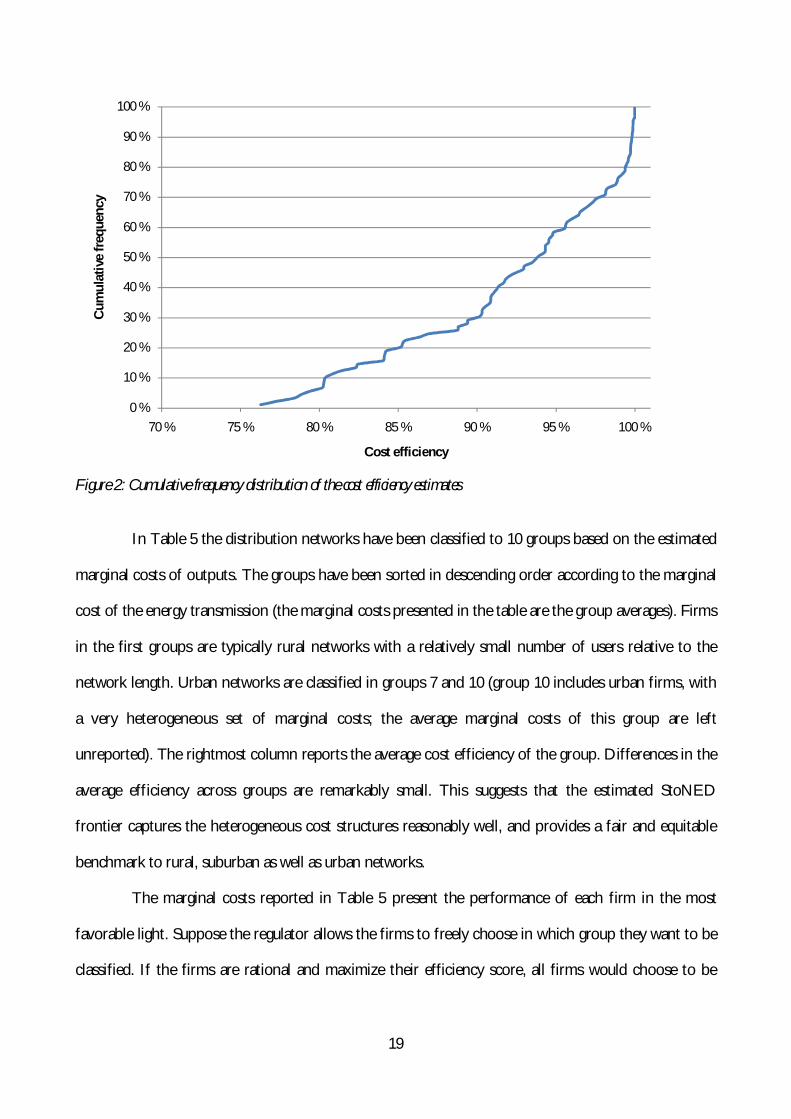
Firm-specific efficiency estimates are based on confidential data, and hence cannot be

reported in this study. To illustrate the distribution of firm-specific estimates, we have plotted the

cumulative frequency distribution of the cost efficiency estimates in Figure 2. The plotted curve

indicates the proportion of distribution networks (on the vertical axis) that achieves at least the cost

efficiency level indicated on the horizontal axis (or smaller). For example, 30% of networks operate

with cost efficiency of 90% or less. In other words, 70% of the firms achieve cost efficiency of 90% or

higher. More than 40% of firms operate with cost efficiency of 95% or higher. According to our

estimates, a large majority of the distribution network operate with high degree of cost efficiency.

Unfortunately there are some networks that operate with 80% cost efficiency or lower. In order to

assign more stringent efficiency improvement targets to the least efficient companies, it is crucially

important to be able to isolate inefficiency from the heterogeneity represented by the z variable and

from stochastic noise.

19

Figure 2: Cumulative frequency distribution of the cost efficiency estimates

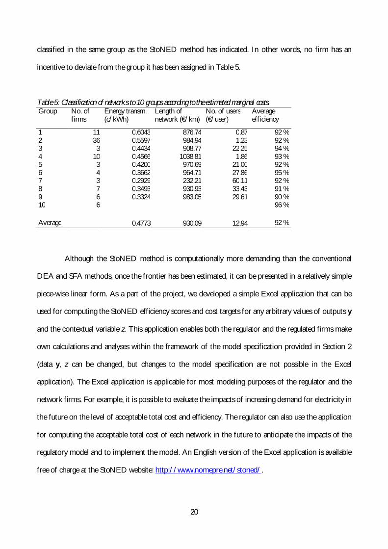
In Table 5 the distribution networks have been classified to 10 groups based on the estimated

marginal costs of outputs. The groups have been sorted in descending order according to the marginal

cost of the energy transmission (the marginal costs presented in the table are the group averages). Firms

in the first groups are typically rural networks with a relatively small number of users relative to the

network length. Urban networks are classified in groups 7 and 10 (group 10 includes urban firms, with

a very heterogeneous set of marginal costs; the average marginal costs of this group are left

unreported). The rightmost column reports the average cost efficiency of the group. Differences in the

average efficiency across groups are remarkably small. This suggests that the estimated StoNED

frontier captures the heterogeneous cost structures reasonably well, and provides a fair and equitable

benchmark to rural, suburban as well as urban networks.

The marginal costs reported in Table 5 present the performance of each firm in the most

favorable light. Suppose the regulator allows the firms to freely choose in which group they want to be

classified. If the firms are rational and maximize their efficiency score, all firms would choose to be

0 %

10 %

20 %

30 %

40 %

50 %

60 %

70 %

80 %

90 %

100 %

70 % 75 % 80 % 85 % 90 % 95 % 100 %

Cum

ulat

ive

freq

uenc

y

Cost efficiency

20

classified in the same group as the StoNED method has indicated. In other words, no firm has an

incentive to deviate from the group it has been assigned in Table 5.

Table 5: Classification of networks to 10 groups according to the estimated marginal costs. Group No. of

firms Energy transm. (c/kWh)

Length of network (€/km)

No. of users (€/user)

Average efficiency

1 11 0.6043 876.74 0.87 92 % 2 36 0.5597 984.94 1.23 92 % 3 3 0.4434 908.77 22.25 94 % 4 10 0.4566 1038.81 1.86 93 % 5 3 0.4200 970.69 21.00 92 % 6 4 0.3662 964.71 27.86 95 % 7 3 0.2929 232.21 60.11 92 % 8 7 0.3493 930.93 33.43 91 % 9 6 0.3324 983.05 29.61 90 % 10 6 96 %

Average 0.4773 930.09 12.94 92 %

Although the StoNED method is computationally more demanding than the conventional

DEA and SFA methods, once the frontier has been estimated, it can be presented in a relatively simple

piece-wise linear form. As a part of the project, we developed a simple Excel application that can be

used for computing the StoNED efficiency scores and cost targets for any arbitrary values of outputs y

and the contextual variable z. This application enables both the regulator and the regulated firms make

own calculations and analyses within the framework of the model specification provided in Section 2

(data y, z can be changed, but changes to the model specification are not possible in the Excel

application). The Excel application is applicable for most modeling purposes of the regulator and the

network firms. For example, it is possible to evaluate the impacts of increasing demand for electricity in

the future on the level of acceptable total cost and efficiency. The regulator can also use the application

for computing the acceptable total cost of each network in the future to anticipate the impacts of the

regulatory model and to implement the model. An English version of the Excel application is available

free of charge at the StoNED website: http://www.nomepre.net/stoned/.

21

6. Specification tests and sensitivity analysis

6.1 Returns to scale

The StoNED method enables one to test or postulate various specifications regarding the returns to

scale (RTS), similar to DEA. The recommended model specification described in Section 2 is based on

the assumption of constant returns to scale (CRS) that does not allow any premium or advantage for

firms operating at small or large scale. In this sense, the CRS specification treats all firms equally, using

the most productive scale size as a common benchmark to firms of all sizes.

The regulatory model currently used in Finland is based on the assumption of non-decreasing

returns to scale (NDRS). This specification allows small firms to appeal to a disadvantage due to the

small scale, which is compensated in the model by allowing the small firms include a cost premium.

However, large firms are not allowed to have a premium for the diseconomies of scale. The assumption

of NDRS can be justified if the cost function exhibits economies of scale and if the firms cannot

influence the scale. In practice, however, a number of mergers and divisions to smaller companies have

occurred, so the scale of operation is not exogenously given to the firms. If small companies are

allowed a scale premium, it might give the wrong incentives for the firms to avoid mergers that would

improve overall cost efficiency, or even encourage firms to split into smaller and more cost inefficient

companies in order to take advantage of the small-scale premium. From the perspective of regulation,

the specification of the returns to scale should take into account two questions: 1) Does the technology

exhibit economies or diseconomies of scale? 2) Can the firms influence the scale of their operations by

mergers or divisions?

To address the first question, we estimated the cost frontier by the StoNED method under

CRS, NDRS, and variable returns to scale (VRS) specifications. By comparing the distributions of the

regression residuals under the three alternative RTS specifications, we can assess if the returns to scale

specification influences the efficiency estimates. Further, we can test if the impact is statistically

significant.

22

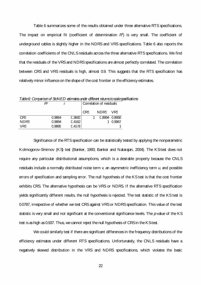
Table 6 summarizes some of the results obtained under three alternative RTS specifications.

The impact on empirical fit (coefficient of determination R2) is very small. The coefficient of

underground cables is slightly higher in the NDRS and VRS specifications. Table 6 also reports the

correlation coefficients of the CNLS residuals across the three alternative RTS specifications. We find

that the residuals of the VRS and NDRS specifications are almost perfectly correlated. The correlation

between CRS and VRS residuals is high, almost 0.9. This suggests that the RTS specification has

relatively minor influence on the shape of the cost frontier or the efficiency estimates.

Table 6: Comparison of StoNED estimates under different returns to scale specifications R2

Correlation of residuals

CRS NDRS VRS CRS 0.9864 0.3600 1 0.8994 0.8958 NDRS 0.9894 0.4162 1 0.9967 VRS 0.9895 0.4178 1

Significance of the RTS specification can be statistically tested by applying the nonparametric

Kolmogorov-Smirnov (KS) test (Banker, 1993; Banker and Natarajan, 2004). The KS-test does not

require any particular distributional assumptions, which is a desirable property because the CNLS

residuals include a normally distributed noise term v, an asymmetric inefficiency term u, and possible

errors of specification and sampling error. The null hypothesis of the KS test is that the cost frontier

exhibits CRS. The alternative hypothesis can be VRS or NDRS. If the alternative RTS specification

yields significantly different results, the null hypothesis is rejected. The test statistic of the KS test is

0.0787, irrespective of whether we test CRS against VRS or NDRS specification. This value of the test

statistic is very small and not significant at the conventional significance levels. The p-value of the KS

test is as high as 0.937. Thus, we cannot reject the null hypothesis of CRS in the KS-test.

We could similarly test if there are significant differences in the frequency distributions of the

efficiency estimates under different RTS specifications. Unfortunately, the CNLS residuals have a

negatively skewed distribution in the VRS and NDRS specifications, which violates the basic

23

assumption of the cost frontier model where the asymmetry of the inefficiency term implies the

residuals of a cost frontier should be positively skewed. The wrong skewness occurs frequently in the

estimation of stochastic frontier models, irrespective of whether one uses conventional SFA or the

proposed StoNED method, or whether one uses a maximum likelihood or least squares estimator.

According to Greene (2008), the wrong skewness can be seen as a built-in diagnostic test: wrong

skewness may be a sign of model misspecification. In the present setting, imposing VRS or NDRS

specification if the underlying technology exhibits CRS could explain the wrong skewness. On the

other hand, Monte Carlo simulations suggest that the wrong skewness occurs with a relatively high

frequency also in correctly specified models. In any case, it is impossible to estimate the cost frontier or

the efficiency estimates under the VRS and NDRS specifications, so we resort to the CRS specification.

As noted before, the StoNED cost frontier under CRS specification explains more than 98%

of the variation in the logarithm of total cost across the firms. Relaxing the CRS assumption improves

the empirical fit only about 0.3 percentage points. Applying the conventional F-test, it is clear that such

a marginal increase in the empirical fit is statistically insignificant even if it cost only one additional

degree of freedom (in fact, the VRS specification involves 89 additional parameters). Regarding the

economic significance, the estimated cost due to the diseconomies of scale amounts to 7.7 Million € in

the NDRS specification. For comparison, the total cost of all firms was 747 Million, so the economic

significance of the RTS specification is only approximately 1 percent of the total cost.

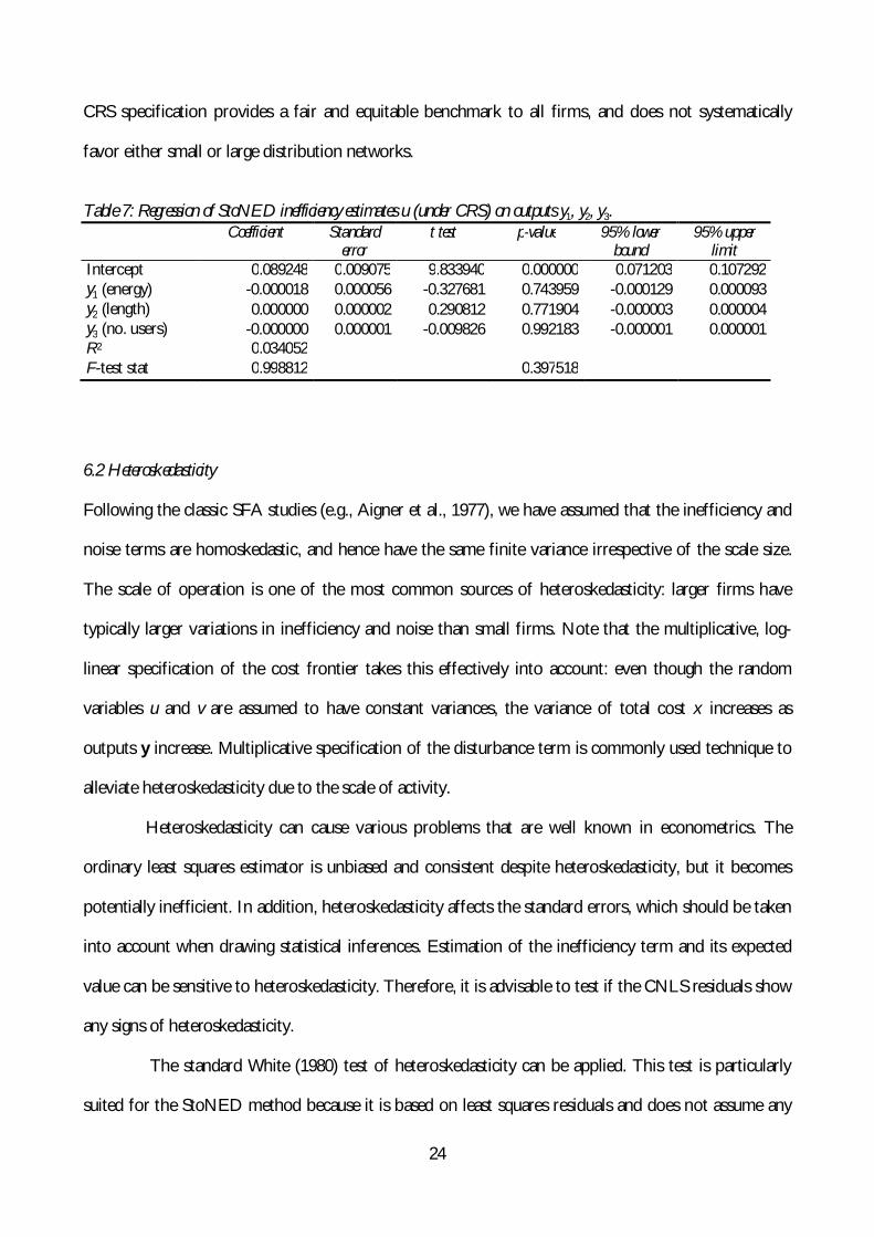
Finally, we can assess whether firms operating with different scale have some advantage or

disadvantage by regressing the inefficiency estimates u obtained in the CRS specification on the three

outputs y1, y2, and y3. The regression results are reported in Table 7 below. We find the coefficients of

all three outputs are close to zero and statistically insignificant. The model as a whole is not jointly

significant according to the F-test.

In conclusion, we cannot reject the CRS hypothesis in the statistical KS-test. Further, the size

of the firm does not explain the efficiency differences across firms. Therefore, we conclude that the

24

CRS specification provides a fair and equitable benchmark to all firms, and does not systematically

favor either small or large distribution networks.

Table 7: Regression of StoNED inefficiency estimates u (under CRS) on outputs y1, y2, y3.

Coefficient Standard error

t test p-value 95% lower bound

95% upper limit

Intercept 0.089248 0.009075 9.833940 0.000000 0.071203 0.107292 y1 (energy) -0.000018 0.000056 -0.327681 0.743959 -0.000129 0.000093 y2 (length) 0.000000 0.000002 0.290812 0.771904 -0.000003 0.000004 y3 (no. users) -0.000000 0.000001 -0.009826 0.992183 -0.000001 0.000001 R2 0.034052 F-test stat 0.998812 0.397518

6.2 Heteroskedasticity

Following the classic SFA studies (e.g., Aigner et al., 1977), we have assumed that the inefficiency and

noise terms are homoskedastic, and hence have the same finite variance irrespective of the scale size.

The scale of operation is one of the most common sources of heteroskedasticity: larger firms have

typically larger variations in inefficiency and noise than small firms. Note that the multiplicative, log-

linear specification of the cost frontier takes this effectively into account: even though the random

variables u and v are assumed to have constant variances, the variance of total cost x increases as

outputs y increase. Multiplicative specification of the disturbance term is commonly used technique to

alleviate heteroskedasticity due to the scale of activity.

Heteroskedasticity can cause various problems that are well known in econometrics. The

ordinary least squares estimator is unbiased and consistent despite heteroskedasticity, but it becomes

potentially inefficient. In addition, heteroskedasticity affects the standard errors, which should be taken

into account when drawing statistical inferences. Estimation of the inefficiency term and its expected

value can be sensitive to heteroskedasticity. Therefore, it is advisable to test if the CNLS residuals show

any signs of heteroskedasticity.

The standard White (1980) test of heteroskedasticity can be applied. This test is particularly

suited for the StoNED method because it is based on least squares residuals and does not assume any

25

particular model or specification of heteroskedasticity. The null hypothesis of the White test is

homoskedasticity. The test is based on an auxiliary regression where we regress the squared residuals on

outputs y, the squared outputs, and their cross-products. If the auxiliary regression can explain the

squared residuals, the null hypothesis is rejected. The White test statistic is defined as nR2. Under the

null hypothesis, this test statistic has the 2 distribution with the degrees of freedom equal to the

number of slope coefficients in the auxiliary regression model (here 9).

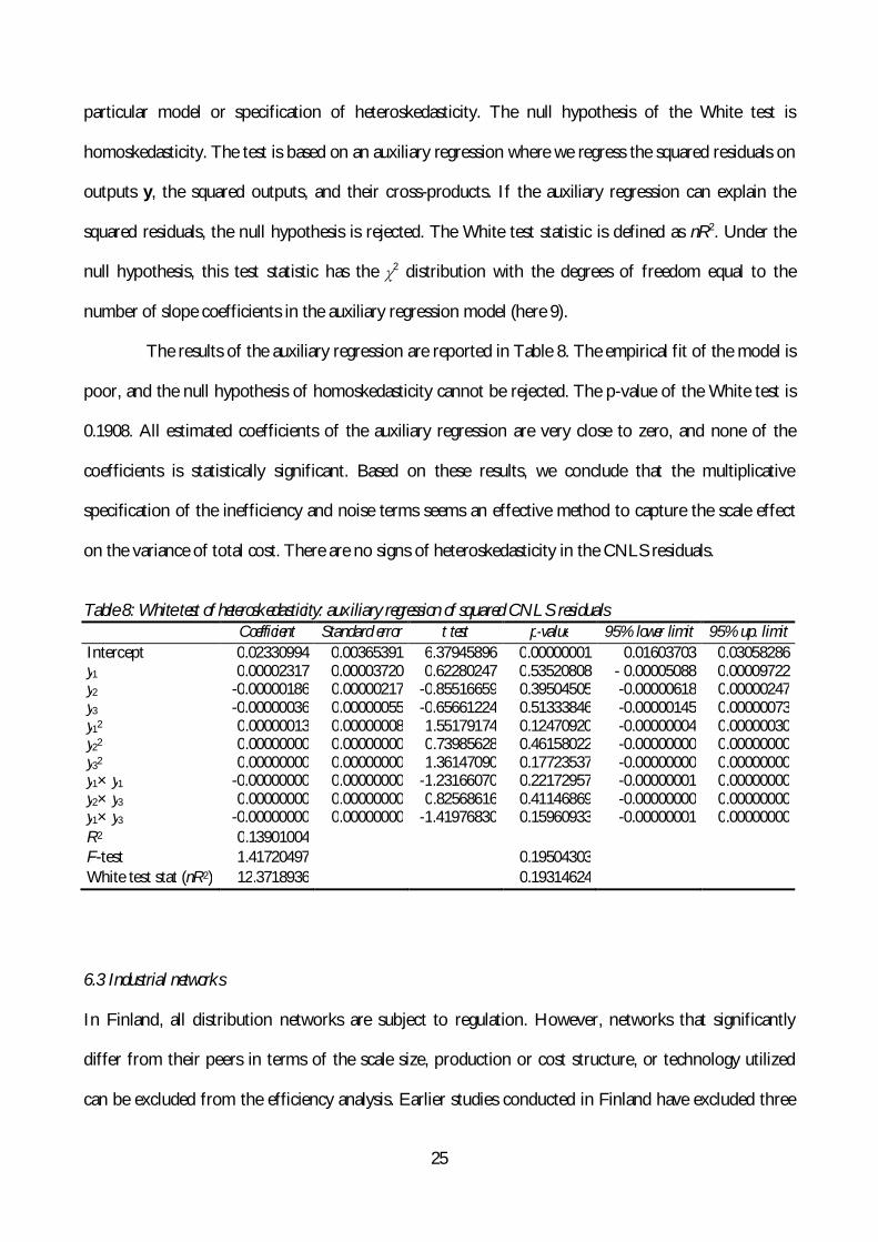
The results of the auxiliary regression are reported in Table 8. The empirical fit of the model is

poor, and the null hypothesis of homoskedasticity cannot be rejected. The p-value of the White test is

0.1908. All estimated coefficients of the auxiliary regression are very close to zero, and none of the

coefficients is statistically significant. Based on these results, we conclude that the multiplicative

specification of the inefficiency and noise terms seems an effective method to capture the scale effect

on the variance of total cost. There are no signs of heteroskedasticity in the CNLS residuals.

Table 8: White test of heteroskedasticity: auxiliary regression of squared CNLS residuals

Coefficient Standard error t test p-value 95% lower limit 95% up. limit Intercept 0.02330994 0.00365391 6.37945896 0.00000001 0.01603703 0.03058286 y1 0.00002317 0.00003720 0.62280247 0.53520808 - 0.00005088 0.00009722 y2 -0.00000186 0.00000217 -0.85516659 0.39504505 -0.00000618 0.00000247 y3 -0.00000036 0.00000055 -0.65661224 0.51333846 -0.00000145 0.00000073 y12 0.00000013 0.00000008 1.55179174 0.12470920 -0.00000004 0.00000030 y22 0.00000000 0.00000000 0.73985628 0.46158022 -0.00000000 0.00000000 y32 0.00000000 0.00000000 1.36147090 0.17723537 -0.00000000 0.00000000 y1× y1 -0.00000000 0.00000000 -1.23166070 0.22172957 -0.00000001 0.00000000 y2× y3 0.00000000 0.00000000 0.82568616 0.41146869 -0.00000000 0.00000000 y1× y3 -0.00000000 0.00000000 -1.41976830 0.15960933 -0.00000001 0.00000000 R2 0.13901004 F-test 1.41720497 0.19504303 White test stat (nR2) 12.3718936 0.19314624

6.3 Industrial networks

In Finland, all distribution networks are subject to regulation. However, networks that significantly

differ from their peers in terms of the scale size, production or cost structure, or technology utilized

can be excluded from the efficiency analysis. Earlier studies conducted in Finland have excluded three

26

so-called industrial networks that mainly focus on distributing power to heavy manufacturing. In Figure

1 these three firms are located on the top of the frontier, with a relatively large amount of distributed

energy, short network length, and small number of customers. In the deterministic DEA method such

atypical observations with a special output profile can have a major influence on the shape of the cost

frontier and the efficiency estimates.

To assess the sensitivity of the StoNED estimates on the impacts of three industrial networks,

we have estimated the recommended model specification with and without the three industrial

networks. For other firms, the correlation of the CNLS residuals between the two model specifications

is very high (0.9933). Correlation of the inefficiency estimates u is almost as high (0.9927). Average cost

efficiency of other networks is 91.11% when the industrial networks are excluded from analysis. When

the industrial networks are included, the average efficiency increases to 91.36%.

In conclusion, the StoNED cost frontier and the related efficiency estimates are not

particularly sensitive to inclusion or exclusion of the three industrial networks, which have a rather

atypical output structure. Interestingly, other networks are slightly better off if the industrial networks

are included in the analysis than if they are excluded. By investigating the efficiency estimates, we find

that one of the industrial networks is highly efficient, whereas the other two industrial networks are

relatively inefficient. On average, cost efficiency of industrial networks slightly lower than that of the

other distribution networks. This explains why excluding the industrial networks does not increase the

estimated efficiency of other networks.

In contrast to DEA that estimates the frontier based on a relatively small number of extreme

observations, the StoNED frontier utilizes information of all n observations in the sample. This is why

the impacts of leaving out a single observation, even a firm with an unusual output structure, are likely

to be small. The relative robustness of the StoNED method to individual observations is an attractive

property in the regulation of a sector where regulated firms merge or split.

27

7. Conclusions and policy recommendations

Based on the results of the project, the final report by Kuosmanen et al. (2010) recommends the

Finnish regulator EMV to replace the currently used DEA and SFA method by the cost frontier

estimated using the StoNED method. The key advantages of the StoNED method include:

1) The stochastic noise is modeled explicitly in a probabilistic manner.

2) Heterogeneity of the firms and their operating environments is taken into account.

3) Conventional statistical tests and confidence intervals can be applied.

4) The method is relatively user-friendly compared to other semi-parametric alternatives.

In the following we briefly elaborate the previous four points.

1) The StoNED method is based on regression analysis, specifically, convex nonparametric

least squares. The stochastic noise is attributed to the regression residual similar to the conventional

regression analysis. As Kuosmanen and Johnson (2010) have shown, the classic DEA estimator is

obtained as a constrained special case of the convex nonparametric least squares regression. Therefore,

the DEA and SFA methods currently used by EMV are both restricted special cases of the more

general StoNED method.

2) Observed heterogeneity of firms and their operating environments can be taken into

account in the StoNED model by using contextual variables. Johnson and Kuosmanen (2009) have

shown that the estimated coefficients of contextual variables are statistically consistent, asymptotically

efficient, asymptotically normally distributed, and converge at the same parametric rate as the

conventional regression coefficients. Thus, the curse of dimensionality that causes problems for the

inference in the second stage regression of conventional DEA efficiency estimates is not a problem in

the StoNED method: precision of the estimator is not affected even if one uses several contextual

variables to describe the operational conditions or practices of the evaluated firms.

3) The probabilistic nature of the StoNED method makes reliable statistical inferences

relatively easy. For example, confidence intervals of the firm specific efficiency scores can be estimated

analogous to the SFA method. Further, it is possible to test for the statistical significance of the

28

efficiency differences across firms or groups of firms (Kuosmanen and Fosgerau, 2009). Statistical

significance of the contextual variables can be tested by the conventional t-test, without

computationally demanding bootstrap simulations. Specification tests such as testing the returns to

scale specification are also available (see Section 6.1). In regulatory applications, reliable statistical tests

are critically important for justifying the model specification and efficiency estimates used in the real-

world regulation.

4) StoNED method builds directly upon the basic assumptions and axioms of DEA and SFA,

and it does not require any additional assumptions or tools. This makes the StoNED method relatively

used-friendly compared to other semi- and non-parametric alternatives available in the literature. The

StoNED method does not require computationally intensive bootstrap simulations or kernel

estimation, and it is conceptually easy to master based on the conventional DEA and SFA. Solving the

nonparametric least squares problem requires sufficient hardware resources and a proper solver for

quadratic or nonlinear programming, but once the StoNED frontier has been estimated, computing

cost targets or reference points on the frontier is easy. As a part of the project we developed a simple

Excel-spreadsheet to enable EMV and the regulated power companies make their own efficiency

analyses using the estimated StoNED frontier. One can insert existing or forecasted values of outputs

and costs, and the Excel-spreadsheet will automatically compute the efficient cost level and the

efficiency improvement target in percents and Euro based on the StoNED cost frontier and the

inserted cost.

In conclusion, the method proves well suited the purposes of the cost efficiency estimation in

the regulatory model that EMV applies in Finland. It provides several distinct advantages compared to

the conventional DEA and SFA methods currently used. We believe the StoNED method could be an

interesting alternative for the regulatory applications world-wide, not only in electricity distribution but

in the regulation of local monopolies in general.

29

References Agrell P., P. Bogetoft & J.Tind (2005): “DEA and Dynamic Yardstick Competition in Scandinavian Electricity

Distribution,” Journal of Productivity Analysis 23, 173–201.

Aigner, D.J., C.A.K. Lovell, & P. Schmidt (1977): “Formulation and Estimation of Stochastic Frontier Models,”

Journal of Econometrics 6, 21-37.

Banker, R.D. (1993): “Maximum Likelihood, Consistency and Data Envelopment Analysis: A Statistical

Foundation,” Management Science 39(10), 1265-1273.

Banker, R.D. & R. Natarajan (2004): ”Statistical Tests Based on DEA Efficiency Scores,” Luku 11 teoksessa

W.W. Cooper, L. Seiford & J. Zhu (Eds.): Handbook on Data Envelopment Analysis, Kluwer Academic

Publishers, Norwell, MA, pp. 299-321.

Charnes, A., W.W. Cooper & E. Rhodes. (1978): “Measuring the Efficiency of Decision Making Units,” European

Journal of Operational Research 2: 429-44.

Cullmann, A. & C. von Hirschhausen (2008): “From Transition to Competition - Dynamic Efficiency Analysis

of Polish Electricity Distribution,” Economics of Transition 16(2):335–357.

Edvardsen, D.F. & F.R. Forsund (2003): “International Benchmarking of Electricity Distribution Utilities,”

Resource and Energy Economics 25(4), 353-371.

Estache, A., M.A. Rossi, C.A. Ruzzier (2004): “The Case for International Coordination of Electricity

Regulation: Evidence from the Measurement of Efficiency in South America,” Journal of Regulatory

Economics 25(3), 271-295.

Farrell, M.J. (1957): “The Measurement of Productive Efficiency,” Journal of the Royal Statistical Society A 120: 253-

81.

Filippini, M., N. Hrovatin, & N. Zoric (2004): ”Efficiency and Regulation of the Slovenian Electricity

Distribution Companies, Energy Policy 32, 335-344.

Forsund, F.R. & S.A.C. Kittelsen (1998): ”Productivity Development of Norwegian Electricity Distribution

Utilities,” Resources and Economics 20, 207-224.

Greene W.H. (2008): “The Econometric Approach to Efficiency Analysis,” Ch. 2 in H. Fried, C.A.K. Lovell &

S.S. Schmidt (Eds) The Measurement of Productive Efficiency and Productivity Growth, Oxford University Press.

Hirschhausen, C. von, A. Cullman & A. Kappeler (2006): “Efficiency Analysis of German Electricity

Distribution Utilities: Nonparametric and Parametric Tests,” Applied Economics 38, 2553-2566.

Hjalmarsson, L. & A. Veiderpass (1992): ”Productivity in Swedish Electricity Retail Distribution,” Scandinavian

Journal of Economics 94, 193-205.

Jamasb, T. & M. Pollit (2003): “International Benchmarking and Regulation: An Application to European

Electricity Distribution Utilities,” Energy Policy 31, 1609-1622.

Johnson, A.L., & T. Kuosmanen (2009): “How Operational Conditions and Practices Affect Productive

Performance? Efficient Semi-Parametric One-Stage Estimators,” SSRN working paper (available

online at http://ssrn.com/abstract=1485733).

Jondrow, J., C.A.K. Lovell, I.S. Materov & P. Schmidt (1982): “On the Estimation of Technical Inefficiency in

the Stochastic Frontier Production Function Model,” Journal of Econometrics 19(2-3): 233-238.

30

Kopsakangas-Savolainen, M. & R. Svento (2008): “Estimation of Cost-Effectiveness of the Finnish Electricity

Distribution Utilities,” Energy Economics 30(2): 212-229.

Korhonen, P., M. Syrjänen & M. Tötterström (2000): ”Sähkönjakeluverkkotoiminnan kustannus-tehokkuuden

mittaaminen DEA-menetelmällä”. Energiamarkkinaviraston julkaisuja 1/2000 (available online at

www.energiamarkkinavirasto.fi).

Korhonen, P. and M. Syrjänen (2003): “Evaluation of Cost Efficiency in Finnish Electricity Distribution,”Annals

of Operations Research 121, 105-122.

Kuosmanen, T. (2006): “Stochastic Nonparametric Envelopment of Data: Combining Virtues of SFA and DEA

in a Unified Framework”, MTT Discussion Paper No. 3/2006.

Kuosmanen, T. (2008): “Representation Theorem for Convex Nonparametric Least Squares”, Econometrics Journal

11, 308-325.

Kuosmanen, T., & M. Fosgerau (2009): “Neoclassical versus Frontier Production Models? Testing for the

Presence of Inefficiencies in the Regression Residuals”, Scandinavian Journal of Economics 111(2), 317-333.

Kuosmanen, T., & A.L. Johnson (2010): “Data Envelopment Analysis as Nonparametric Least Squares

Regression”, Operations Research 58(1): 149-160.

Kuosmanen, T., & M. Kortelainen (2007): “Stochastic Nonparametric Envelopment of Data: Cross-Sectional

Frontier Estimation Subject to Shape Constraints”, University of Joensuu, Economics Discussion

Paper No. 46.

Kuosmanen, T., M. Kortelainen, K. Kultti, H. Pursiainen, A. Saastamoinen & T. Sipiläinen (2010):

”Sähköverkkotoiminnan kustannustehokkuuden estimointi StoNED-menetelmällä: Ehdotus

tehostamistavoitteiden ja kohtuullisten kustannusten arviointiperusteiden kehittämiseksi kolmannella

valvontajaksolla 2012-2015”, Energiamarkkinaviraston julkaisu 31.8.2010 (available online at

www.energiamarkkinavirasto.fi).

Meeusen, W. & J. van den Broeck (1977): “Efficiency Estimation from Cobb-Douglas Production Function with

Composed Error,” International Economic Review 8, 435-444.

Pahwa, A., X. Feng & D. Lubkeman (2003): ”Performance Evaluation of Electric Distribution Utilities Based on

Data Envelopment Analysis,” IEEE Transactions on Power Systems 18(1), 400-405.

Syrjänen, M., P. Bogetoft, and P. Agrell (2006): “Analogous Efficiency Measurement Model Based on Stochastic Frontier

Analysis.” Gaia Consulting Oy 11.12.2006 (available online at www.energiamarkkinavirasto.fi).

Thakur, T., S.G. Deshmukh, S.C. Kaushik & M. Kulshresta (2005): ”Impact Assessment of the Electricity Act

2003 on the Indian Power Sector,” Energy Policy 33(9), 1187-1198.

Thakur, T., S.G. Deshmukh, & S.C. Kaushik (2007): “Efficiency Evaluation of the State Owned Electricity

Utilities in India, Energy Policy 34(17), 1187-1198.

White, H. (1980): “A Heteroskedasticity-Consistent Covariance Matrix Estimator and a Direct Test for

Heteroskedasticity,” Econometrica 48(4), 817-38.

31

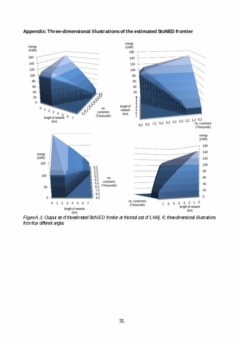
Appendix: Three-dimensional illustrations of the estimated StoNED frontier

Figure A.1: Output set of the estimated StoNED frontier at the total cost of 1 Milj. €; three dimensional illustrations from four different angles.

9,28,2

7,26,2

5,24,23,22,21,20,2

020

40

60

80

100

120

140

160

0 1 2 3 4 5 6 7

no. customers

(Thousands)

energy(GWh)

length of network(km)

9,2 8,2 7,2 6,2 5,2 4,2 3,2 2,2 1,2 0,2

020

40

60

80

100

120

140

160

01234567

no. customers (Thousands)

energy(GWh)

length of network

(km)

9,28,27,26,25,24,23,22,21,20,2

0

50

100

150

0 1 2 3 4 5 6 7

no. customers

(Thousands)

energy(GWh)

length of network(km)

0

20

40

60

80

100

120

140

160

01234567no. custormers (Thousands)

energy(GWh)

length of network(km)