Cost-effective design and operationof variable speed wind turbines

Closing the gap between the control engineering and the windengineering community

Cost-effective design and operationof variable speed wind turbines

Closing the gap between the control engineering and the windengineering community

Proefschrift

ter verkrijging van de graad van doctoraan de Technische Universiteit Delft,

op gezag van de Rector Magnificus prof. dr. ir. J.T. Fokkemavoorzitter van het College voor Promoties,

in het openbaar te verdedigen op dinsdag 18 februari 2003 om 16.00 uurdoor

David-Pieter MOLENAAR

werktuigkundig ingenieurgeboren te Middelie

Dit proefschrift is goedgekeurd door de promotor:Prof. ir. O.H. Bosgra

Samenstelling promotiecommissie:

Rector Magnificus voorzitterProf. ir. O.H. Bosgra Technische Universiteit Delft, promotorDr. Sj. Dijkstra Technische Universiteit Delft, toegevoegd promotorProf. dr. ir. G.A.M. van Kuik Technische Universiteit DelftDr. ir. M.J. Hoeijmakers Technische Universiteit DelftProf. dr. ir. D.J. Rixen Technische Universiteit DelftProf. dr. ir. Th. van Holten Technische Universiteit DelftProf. dr. ir. M. Steinbuch Technische Universiteit Eindhoven

Published and distributed by: DUP Science

DUP Science is an imprint ofDelft University PressP.O. Box 982600 MG DelftThe NetherlandsTelephone: +31 15 27 85 678Telefax: +31 15 27 85 706E-mail: DUP@Library.TUDelft.NL

ISBN 90-407-2383-4

Keywords: variable speed wind turbines, modeling, model validation

Copyright c©2003 by David Molenaar

All rights reserved. No part of the material protected by this copyright notice maybe reproduced or utilized in any form or by any means, electronic or mechanical, in-cluding photocopying, recording or by any information storage and retrieval system,without written permission from the publisher: Delft University Press.

Printed in The Netherlands

For free

and still too

expensive

Voorwoord

Promoveren? Daaf gaat promoveren? Deze reactie kreeg ik 6 jaar geleden vlakna mijn afstuderen te horen. Ik moest zelf ook even aan het idee wennen, maarde uitdaging om uit te zoeken of de stelling “windenergie: gratis en toch duur”ontkrachtigd kon worden sprak mij zeer aan. De vrijheid (en dus de mogelijkheden)bij de sectie Systeem en Regeltechniek om dit doel te bereiken was voor mij debelangrijkste reden om voor de Technische Universiteit Delft en niet voor het ECNin Petten of Stork Product Engineering in Amsterdam te kiezen.

Ik behoor tot de groep promovendi die puur voor het onderwerp gekozen heeft.Windenergie intrigeerde me eigenlijk als kind al. Mijn vader wilde een windmolen inde tuin zetten om elektriciteit op te wekken en dat vond ik zeer interessant. Helaasis dat er nooit van gekomen, hoewel hij er onlangs weer over begon...

Onderzoek doen is leuk (zeker naar windenergie gezien het brede en maatschappelijkekarakter van het onderwerp). Maar helaas, het werk zit erop en dus is het momentgekomen een aantal mensen te bedanken voor hun positieve bijdrage op het verloopvan mijn onderzoek. Van deze groep wil ik de volgende personen graag met naamnoemen.

Allereerst wil ik Maarten Steinbuch bedanken voor het feit dat hij mij het laatstezetje gegeven heeft. Maarten, ik heb er geen moment spijt van gehad! Natuurlijkwas dit project nooit tot stand gekomen als Okko Bosgra mij niet de gelegenheidhad gegeven de traditie op de sectie voort te zetten. Speciale dank gaat ook uit naarGregor van Baars voor het beschikbaar stellen van zijn vrije tijd om de overgangvan student naar promovendus te versoepelen.

Verder wil ik de sectie bedanken voor de stimulerende werkomgeving. In het bijzon-der Sjoerd Dijkstra voor de morele en politieke ondersteuning en Peter Valk voorde soft- en hardware ondersteuning. De “woensdag-after-lunch” presentaties met debijbehorende discussies evenals de (soms onzinnige) bijdragen tijdens de lunch hebik zeer gewaardeerd. Hans, Dick, Joost, Judi, Marco, Edwin, Thomas, Sjirk, Rob,A3, Martijn, Branko, Gideon, Eduard, Camile, Les, Jogchem, Leon, Dennis, Alex,Maria, Maria M., Els, Jacqueline, Marjolein, Debby, Agnes, “kroketten” Cor, Frits,Ton, Guus, John, Ad, Carsten, Peter H. en Paul: bedankt. Daarnaast hebben som-mige afstudeerders op mij een onvergetelijke indruk achter gelaten. Martin, Jurjen,

i

Mario en Mark, ook al staan niet al jullie resultaten vermeld in dit proefschrift, tochbedankt voor jullie (inhoudelijke) bijdragen.

Tijdens mijn promotie heeft een aantal mensen een essentiele bijdrage geleverd aan deexperimenten uitgevoerd op de Lagerwey LW-50/750 windturbine. Andre Pubanz,Martin Hoeijmakers, John Vervelde, Bert Bosman, Jan Lucas, Cees van Everdinck,Rob Tousain, Koert de Kok, Robert Verschuren en Berit van Hulst: bedankt voorjullie inzet en vooral geduld. Zonder jullie zou dit proefschrift minstens de helftdunner en lang niet zo waardevol zijn. Daarnaast wil ik Bart Roorda en HenkHeerkes bedanken voor het beschikbaar stellen van respectievelijk de Polymarin enAERPAC rotorblad gegevens. Tevens wil ik Hans van Leeuwen, Gerben de Winkel,Don van Delft, Arno van Wingerde en Peter Joosse bedanken voor het beschikbaarstellen van de modale testresultaten van diverse rotorbladen en hun assistentie bijhet analyseren van de data.

Vervolgens wil ik Sylvia bedanken voor de altijd gezellige ontvangst op de 6de.Hans en Jan bedankt voor jullie enthousiasme, kritische houding, samenwerking engezelligheid. Ik hoop dat al onze plannen uitkomen en dat in navolging van julliemeer DUWIND-ianen de Mekelweg over durven te steken.

Ik wil Richard Luijendijk (Siemens Nederland N.V.) bedanken voor het feit dat hijmij de mogelijkheid heeft geboden de wind (tijdelijk) vanuit een andere positie tebekijken. In de periode dat ik bij Siemens aan het NSWP (North Sea Wind Power)project gewerkt heb, heb ik veel van jou en onze samenwerking geleerd. Daarnaastheb ik de bevestiging gekregen dat dit proefschrift een belangrijke bijdrage kanleveren in het verbeteren van de concurrentiepositie van windenergie.

Monique: super dat je de omslag van mijn proefschrift hebt willen vormgeven. Ikhoop dat de vormgeving de dikte een beetje compenseert.

Mijn ouders, “Pap en Mam”, hartstikke bedankt voor alle goede zorgen. Zonderjullie steun had ik dit nooit kunnen doen. Wat ik het meest in jullie bewonder is datjullie zowel Dirk-Jacob als mij de ruimte en kans hebben gegeven dingen te doen diejullie vroeger door de andere omstandigheden nooit hebben kunnen doen.

Tenslotte wil ik mijn vriendin Nannila bedanken. Niet alleen voor de liefde en steuntijdens mijn promotie, maar ook voor het af en toe dichtgooien van mijn laptop.

Zo, nu is het weer tijd voor een goed boek,

David-Pieter “Daaf” MolenaarDelft, 1 december 2002.

ii

Note to the reader

Consciousness is raising in the wind engineering community that control designshould be an integral part of the complete wind turbine design. Obviously, thedynamics of a controller interact with the dynamics of the wind turbine and so haveimplications for, among other things, the energy production, fatigue life and the windturbine configuration. In an ideal situation the wind turbine components (includingcontroller) should be designed taking into account their behavior in the completewind turbine. This will lead to an integrated and optimal wind turbine design as wellas optimal operation. It must be emphasized that designing a controller afterwards(i.e. after the turbine has already been constructed) is certainly not cost-effective.

I have tried to make the contents of this thesis to be digestible for readers livingin both the control system community and the wind engineering community in anattempt to reduce the significant gap that exists between the two communities.This lack of fruitful multidisciplinary interaction obviously limits the technologicalimprovements required to achieve economic viability of the use of wind power.

iii

iv

Contents

Voorwoord . . . . . . . . . . . . . . . . . . . . . . . . . . . . . . . . . . . iNote to the reader . . . . . . . . . . . . . . . . . . . . . . . . . . . . . . . iii

1 Introduction 11.1 Motivation and background . . . . . . . . . . . . . . . . . . . . . . . 1

1.1.1 History: from windmill to wind turbine . . . . . . . . . . . . 11.1.2 The future of wind power . . . . . . . . . . . . . . . . . . . . 91.1.3 Cost-effective wind turbine design and operation . . . . . . . 11

1.2 Problem formulation . . . . . . . . . . . . . . . . . . . . . . . . . . . 131.3 Outline . . . . . . . . . . . . . . . . . . . . . . . . . . . . . . . . . . 151.4 Typographical conventions . . . . . . . . . . . . . . . . . . . . . . . . 16

Part I: Modeling of flexible wind turbines 17

2 State-of-the-art of wind turbine design codes 192.1 Introduction . . . . . . . . . . . . . . . . . . . . . . . . . . . . . . . . 192.2 Overview wind turbine design codes . . . . . . . . . . . . . . . . . . 202.3 Main features overview . . . . . . . . . . . . . . . . . . . . . . . . . . 23

2.3.1 Rotor aerodynamics . . . . . . . . . . . . . . . . . . . . . . . 232.3.2 Structural dynamics . . . . . . . . . . . . . . . . . . . . . . . 302.3.3 Generator description . . . . . . . . . . . . . . . . . . . . . . 322.3.4 Wind field description . . . . . . . . . . . . . . . . . . . . . . 332.3.5 Wave field description . . . . . . . . . . . . . . . . . . . . . . 352.3.6 Control design . . . . . . . . . . . . . . . . . . . . . . . . . . 382.3.7 Summary main features in tabular form . . . . . . . . . . . . 39

2.4 Conclusions . . . . . . . . . . . . . . . . . . . . . . . . . . . . . . . . 42

3 Dynamic wind turbine model development 453.1 Introduction: general wind turbine model . . . . . . . . . . . . . . . 453.2 Wind module . . . . . . . . . . . . . . . . . . . . . . . . . . . . . . . 483.3 Aerodynamic module . . . . . . . . . . . . . . . . . . . . . . . . . . . 49

3.3.1 Introduction . . . . . . . . . . . . . . . . . . . . . . . . . . . 493.3.2 Rankine-Froude actuator-disk model . . . . . . . . . . . . . . 493.3.3 Blade element momentum model . . . . . . . . . . . . . . . . 583.3.4 Calculation of the blade element forces . . . . . . . . . . . . . 67

v

3.4 Mechanical module . . . . . . . . . . . . . . . . . . . . . . . . . . . . 693.4.1 Introduction . . . . . . . . . . . . . . . . . . . . . . . . . . . 693.4.2 Superelement approach . . . . . . . . . . . . . . . . . . . . . 723.4.3 Generation of the equations of motion of MBS . . . . . . . . 763.4.4 Automated structural modeling procedure . . . . . . . . . . . 793.4.5 Soil dynamics . . . . . . . . . . . . . . . . . . . . . . . . . . . 803.4.6 Example: three bladed wind turbine . . . . . . . . . . . . . . 82

3.5 Electrical module . . . . . . . . . . . . . . . . . . . . . . . . . . . . . 833.5.1 Introduction . . . . . . . . . . . . . . . . . . . . . . . . . . . 833.5.2 Synchronous generator: physical description . . . . . . . . . . 843.5.3 Synchronous generator: mathematical description . . . . . . . 873.5.4 Dynamic generator model . . . . . . . . . . . . . . . . . . . . 87

3.6 Summary . . . . . . . . . . . . . . . . . . . . . . . . . . . . . . . . . 103

Part II: Model validation issues 107

4 Module verification and validation 1094.1 Introduction . . . . . . . . . . . . . . . . . . . . . . . . . . . . . . . . 109

4.1.1 Verification versus validation . . . . . . . . . . . . . . . . . . 1104.1.2 Model verification and validation approach . . . . . . . . . . 111

4.2 Mechanical module verification and validation . . . . . . . . . . . . . 1124.2.1 Case 1: Euler-Bernoulli beam (verification) . . . . . . . . . . 1124.2.2 Case 2: APX-45 rotor blade (validation) . . . . . . . . . . . . 1204.2.3 Case 3: APX-70 rotor blade (validation) . . . . . . . . . . . . 1244.2.4 Case 4: RB-51 rotor blade (validation) . . . . . . . . . . . . . 1264.2.5 Case 5: RB-70 rotor blade (validation) . . . . . . . . . . . . . 1264.2.6 Discussion . . . . . . . . . . . . . . . . . . . . . . . . . . . . . 1284.2.7 Case 6: Lagerwey LW-50/750 wind turbine . . . . . . . . . . 131

4.3 Electrical module verification and validation . . . . . . . . . . . . . . 1424.3.1 Literature review . . . . . . . . . . . . . . . . . . . . . . . . . 1424.3.2 Synchronous generator parameter identification . . . . . . . . 1424.3.3 MSR test applied to the LW-50/750 generator . . . . . . . . 147

4.4 Conclusions . . . . . . . . . . . . . . . . . . . . . . . . . . . . . . . . 156

5 Model parameter updating using time-domain data 1595.1 Introduction . . . . . . . . . . . . . . . . . . . . . . . . . . . . . . . . 1595.2 Identifiability of model parameters . . . . . . . . . . . . . . . . . . . 161

5.2.1 Persistence of excitation . . . . . . . . . . . . . . . . . . . . . 1625.2.2 Model parametrization . . . . . . . . . . . . . . . . . . . . . . 163

5.3 Off-line parameter optimization procedure . . . . . . . . . . . . . . . 1655.3.1 Unconstrained optimization . . . . . . . . . . . . . . . . . . . 1655.3.2 Constrained optimization . . . . . . . . . . . . . . . . . . . . 1695.3.3 Selecting a method . . . . . . . . . . . . . . . . . . . . . . . . 169

5.4 Verification using simulated data . . . . . . . . . . . . . . . . . . . . 1715.4.1 Beam1sd . . . . . . . . . . . . . . . . . . . . . . . . . . . . . 1715.4.2 SDLW1 . . . . . . . . . . . . . . . . . . . . . . . . . . . . . . 177

vi

5.5 Discussion . . . . . . . . . . . . . . . . . . . . . . . . . . . . . . . . . 180

Part III: Model based control design 183

6 Frequency converter controller design 1856.1 Introduction . . . . . . . . . . . . . . . . . . . . . . . . . . . . . . . . 1856.2 Frequency converter controller objectives . . . . . . . . . . . . . . . . 1866.3 Frequency converter controller configuration . . . . . . . . . . . . . . 187

6.3.1 Rectifier controller . . . . . . . . . . . . . . . . . . . . . . . . 1886.3.2 Inverter controller . . . . . . . . . . . . . . . . . . . . . . . . 191

6.4 Rectifier frequency converter controller design . . . . . . . . . . . . . 1916.4.1 Open-loop analysis . . . . . . . . . . . . . . . . . . . . . . . . 1916.4.2 Set-point computation and controller design . . . . . . . . . . 1926.4.3 Closed-loop analysis . . . . . . . . . . . . . . . . . . . . . . . 194

6.5 Conclusions . . . . . . . . . . . . . . . . . . . . . . . . . . . . . . . . 194

7 Economic control design 1977.1 Introduction . . . . . . . . . . . . . . . . . . . . . . . . . . . . . . . . 1977.2 Closed-loop wind turbine control . . . . . . . . . . . . . . . . . . . . 198

7.2.1 History of windmill and wind turbine control . . . . . . . . . 1987.2.2 State-of-the-art variable speed wind turbine control . . . . . 200

7.3 The cost of generating electricity using wind . . . . . . . . . . . . . . 2037.3.1 Performance increase . . . . . . . . . . . . . . . . . . . . . . . 2047.3.2 Cost reduction . . . . . . . . . . . . . . . . . . . . . . . . . . 205

7.4 Closed-loop control design methodology: design guidelines . . . . . . 206

Part IV: Conclusions and recommendations 207

8 Conclusions 209

9 Recommendations for future research 213

Part V: Appendices 217

A Main features Lagerwey LW-50/750 wind turbine 219A.1 The Lagerwey LW-50/750 wind turbine . . . . . . . . . . . . . . . . 219A.2 Rotor . . . . . . . . . . . . . . . . . . . . . . . . . . . . . . . . . . . 220A.3 Support structure . . . . . . . . . . . . . . . . . . . . . . . . . . . . . 224A.4 Generator . . . . . . . . . . . . . . . . . . . . . . . . . . . . . . . . . 225

B Flow states of a wind turbine rotor 227

C Comparison of the finite element, lumped-mass and superelementmethod 231C.1 Exact eigenfrequencies . . . . . . . . . . . . . . . . . . . . . . . . . . 231C.2 Finite Element approximation . . . . . . . . . . . . . . . . . . . . . . 232C.3 Lumped-mass approximation . . . . . . . . . . . . . . . . . . . . . . 233

vii

C.4 Superelement approximation . . . . . . . . . . . . . . . . . . . . . . 234C.5 Comparison . . . . . . . . . . . . . . . . . . . . . . . . . . . . . . . . 234

D Proofs of Section 3.5 237D.1 Direct-axis . . . . . . . . . . . . . . . . . . . . . . . . . . . . . . . . . 237D.2 Quadrature-axis . . . . . . . . . . . . . . . . . . . . . . . . . . . . . 242

E Main wind turbine modes of operation 245

F Modal analysis measurement equipment 247F.1 Cable . . . . . . . . . . . . . . . . . . . . . . . . . . . . . . . . . . . 247F.2 Data acquisition system . . . . . . . . . . . . . . . . . . . . . . . . . 248F.3 Force transducer . . . . . . . . . . . . . . . . . . . . . . . . . . . . . 249F.4 Accelerometers . . . . . . . . . . . . . . . . . . . . . . . . . . . . . . 250

F.4.1 Accelerometer mounting . . . . . . . . . . . . . . . . . . . . . 250F.4.2 Accelerometer positions . . . . . . . . . . . . . . . . . . . . . 251

G Frequency response functions 253G.1 Single degree of freedom . . . . . . . . . . . . . . . . . . . . . . . . . 253G.2 Two degrees of freedom . . . . . . . . . . . . . . . . . . . . . . . . . 257

H Modified step-response test measurement equipment 263H.1 Generator . . . . . . . . . . . . . . . . . . . . . . . . . . . . . . . . . 263H.2 Transfoshunt . . . . . . . . . . . . . . . . . . . . . . . . . . . . . . . 264H.3 Low power DC voltage source . . . . . . . . . . . . . . . . . . . . . . 264H.4 Thyristor . . . . . . . . . . . . . . . . . . . . . . . . . . . . . . . . . 264H.5 Data-acquisition system . . . . . . . . . . . . . . . . . . . . . . . . . 264

H.5.1 Input-output boards . . . . . . . . . . . . . . . . . . . . . . . 265H.5.2 Digital Signal Processor (DSP) board . . . . . . . . . . . . . 265H.5.3 Personal computer . . . . . . . . . . . . . . . . . . . . . . . . 266

I DAWIDUM: a new wind turbine design code 267I.1 Introduction . . . . . . . . . . . . . . . . . . . . . . . . . . . . . . . . 267I.2 Modeling . . . . . . . . . . . . . . . . . . . . . . . . . . . . . . . . . 269

I.2.1 Wind module library . . . . . . . . . . . . . . . . . . . . . . . 269I.2.2 Aerodynamic module library . . . . . . . . . . . . . . . . . . 271I.2.3 Mechanical module library . . . . . . . . . . . . . . . . . . . 272I.2.4 Electrical module library . . . . . . . . . . . . . . . . . . . . 278

Bibliography 279

Definitions 305

Glossary of symbols 313

Index 325

viii

Samenvatting 333

Abstract 335

Curriculum vitae 337

ix

x

Chapter 1

Introduction

In the 1970s the concern about the limited fossil fuel resources and their impact onthe environment awakened. Due to this growing concern, interest revived in usingrenewable energy sources in order to meet the constantly rising world electricitydemand. In addition, the oil crises of 1973 and 1979 led to the awareness that theamount of energy import should be decreased so as to become less dependent of oilexporting countries. The Gulf-war (1990-1991) confirmed this concern. One way touse renewable energy sources is to generate electricity using wind turbines.

1.1 Motivation and background

The wind is a vast, worldwide renewable source of energy. Since ancient times,mankind has harnessed the power of the wind. The earliest known use of wind poweris the sailboat. Wind energy propelled boats sailed up the Nile against the current asearly as 5000 B.C. By 1000 A.D. the Vikings had explored and conquered the NorthAtlantic. The wind was also the driving force behind the voyages of discovery ofthe Verenigde Oost-Indische Compagnie (VOC) between 1602 and 1799. Windmillshave been providing useful mechanical power for at least the last thousand years,while wind turbines generate electricity since 1888.

1.1.1 History: from windmill to wind turbine

The historic development of using wind as a source of power shows an evolutionfrom simple drag-type vertical-axis windmills generating mechanical power for localuse, via stand-alone wind turbines designed for battery charging and single grid-connected wind turbines producing AC power using aerodynamic lift, to wind farmssupplying electricity to the utility grid for distribution to the consumers. In thissubsection we shall briefly review this transition from windmills to wind turbines.The next subsection presents an outlook on the future of wind power. Finally, therequired improvements in both wind turbine design and operation to achieve andmaintain cost-effective wind turbines are discussed.

1

1000 A.D. - 1180 A.D.

The first windmills were developed to automate the tasks of grain-grinding andwater-pumping. Although the Chinese reportedly invented the windmill, the earliest-documented design is the vertical-axis windmill used in the region Sıstan in easternPersia for grinding grain and hulling rice in the tenth century A.D. [279]. One ofthe most important climatic features of this extensive border region of present dayAfghanistan and Iran is a northerly wind that blows unceasingly during the summermonths of June to September at velocities ranging between 27 and 47 meters persecond. This wind is locally referred to as “the wind of 120 days”.

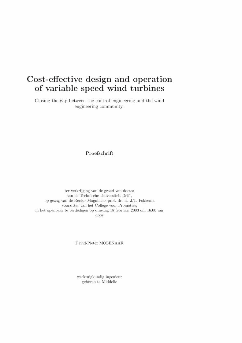
The Persian windmills were usually laid out in a single line that was built at thetop of a mountain, hill or tower with high walls separating them as illustrated inFig. 1.1 [321]. The famous example near the town of Neh had one line of 75 wind-mills. The lines were oriented perpendicular to the prevailing wind direction. Eachindividual windmill consisted of a two-storey structure made of sun-dried bricks.The upper part of the structure contained the millstones (about 2 m in diameter),while the lower part contained a vertical spindle (or wind-wheel) which was fittedwith between six and twelve radial arms as illustrated in Fig. 1.2. Each of these armswas covered with fabric that is allowed to bulge in order to catch the wind. In thewalls of the lower part containing the wind-wheel were apertures being aligned withthe primary wind direction. As a consequence, this kind of windmill can only workin a region where there is a steady prevailing wind. The apertures were wider on theoutside than on the inside, forcing the wind to increase its velocity as it enters thewheel-house and rotate the wind-wheel, which then directly drives the millstones. Inaddition, a series of shutters were used (presumably on the outside of the structure)to admit or shut out the wind, and thereby regulate the rotational speed.

Figure 1.1: Left photograph: Downwind view of a vertical-axis windmill of the Per-sian type in the town of Neh. Right photograph: Close-up view of the working surfacemade of bundles of reed [321]. Reprinted by permission of The MIT Press.

2

Figure 1.2: Cross-section of the wind-wheel of a Persian windmill showing the aper-tures being aligned with the primary wind direction.

Vertical-axis windmills of this basic design were still operating in Iran in 1977(and may be still used today) [105]. This means that the basic design has lastedat least 1000 years, although a major change has taken place: the millstones havebeen placed below the rotor as already shown in Fig. 1.1. The advantage of havingthe sails above the millstones was that the working surface could be substantiallyenlarged. Another noticeable change is the use of bundles of reeds instead of fabricto provide the working surface. It must be noted that the Persian windmill nevercame into use in Northwest Europe.

1180 A.D. - 1888 A.D.

The history of the Western windmill begins with the first documented appearanceof the European or “Dutch” windmill in Normandy, France in the year 1180 [80].The “Dutch” windmill had four sails and was of the horizontal-axis configuration.Wooden cog-and-ring gears were used to translate the motion of the horizontal-axisto a vertical movement to turn a grindstone. The reason for the sudden evolutionfrom the vertical-axis Persian design is unknown, but the fact that European waterwheels also had a horizontal-axis configuration – and apparently served as the tech-nological model for the early windmills – may provide part of the answer. Anotherreason may have been the higher structural efficiency of drag-type horizontal ma-chines over drag-type vertical machines. In addition, the omnidirectional wind, asopposed to the Sıstan environment, may have called for an adaptation to suit theconditions.

Windmills spread rapidly throughout Europe in the thirteenth century. In arelatively short time, tens of thousands were in use for a variety of duties. The ap-plications ranged from grinding grain, shredding tobacco, sawing timber, processingspices and paint pigments, milling flax, pressing oil or pumping water for polderdrainage. The performance increased greatly between the twelfth and nineteenth

3

century with the introduction of metal parts. A primary improvement of the Eu-ropean windmills was their designer’s use of sails that generated aerodynamic lift.This feature provided improved rotor efficiency compared with the Persian mills byallowing an increase in rotor speed, which also allowed for superior grinding as wellas pumping action.

The lower cost of wind power to water power and the fact that more sites wereavailable for windmills than there were for water mills caused an increase in the useof windmills. In The Netherlands, this growth contributed to the country’s goldenage (from 1590 till about 1670). As late as 1850, 90% of the power used in Dutchindustry came from the wind. Steam supplied the rest. Industrialization, first inEurope and later in America, led to a gradual decline in the use of windmills. Thesteam engine took over the tasks previously performed by windmills.

In 1896, at the height of the industrial revolution, wind still pumped 41% ofthe polders in The Netherlands. However, in 1904, wind provided only 11% ofDutch industrial energy. These windmills had a rotor diameter and hub height of25 m and 30 m respectively, and were capable of producing the equivalent of 25–50 kW in mechanical form. For comparison, modern wind turbines of the samesize are capable of extracting ten times more power from the wind [80]. As steampower developed, the uncertain power of the wind became less and less economic(in particular after cheap coal came available), and we are left today with a tinyfraction of the elegant structures that once extracted power from the wind. Theseremaining windmills, scattered throughout the world, are a historic, and certainlyvery photogenic, reminder of a past technological age.

1888 A.D. - 1973 A.D.

The first wind turbine to harness the wind for the generation of electricity wasbuilt by Charles F. Brush in Cleveland, Ohio, USA in 1888. The so-called “Brush”windmill was featured with a 17-m diameter multi-blade rotor mounted on an 18-m high rectangular tower as illustrated in Fig. 1.3. The upwind rotor consistedof 144 thin wooden blades, and a large fantail to turn the rotor out of the wind.The turbine was equipped with a 12 kW direct-current generator, and a belt-and-pulley transmission with a step-up ratio of (50:1). The DC generator was locatedon the basement of the tower. The power output was used for charging storagebatteries. Despite its relative success in operating for 20 years, the Brush windmilldemonstrated the limitations of the low-speed, high-solidity rotor for the generationof electricity [279].

The next important step in the transition from windmills to wind turbines wastaken by P. la Cour in 1891 in Askow, Denmark. He developed the first variable speedwind turbine that incorporated the aerodynamic design principles (low-solidity, four-bladed rotors incorporating primitive airfoil shapes and blade twist) used in the bestDutch windmills. The resulting higher speed of the La Cour rotor made this typeof wind turbine quite practical for electricity generation.

By the late 1930s, the pioneering machines of Brush and La Cour had evolvedinto two- or three bladed horizontal-axis wind turbines with the rotor upwind of thetower and low solidity, using a tail vane to position the rotor at right angles with

4

Figure 1.3: “The windmill dynamo and electric light plant of Mr. Charles F. Brush”,Scientific American, December 20, 1890. Copy of an original in the Department ofSpecial Collections, Case Western Reserve University Library Cleveland, Ohio.

the wind direction. The majority of these direct-current producing turbines wereoperated at variable speed with fixed pitch angle rotor blades. The turbines weregenerally reliable and long-lived machines giving reasonable maintenance. They didnot, however, have the cost-effectiveness and capacity to compete with conventionalpower systems.

The majority of the wind turbines built before 1970 were small machines de-signed for battery charging. The 1.25 MW Smith-Putnam wind turbine constituteda notable exception. This constant speed turbine, built in 1941, had a two-bladedrotor of 53.3-meter diameter mounted on a 33.5 m high truss tower. It featuredfull-span active control of the blade pitch angle using a fly-ball governor, active yawcontrol by means of a servomotor, and flapping hinges to reduce gyroscopic loadson the rotor shaft. The turbine was erected on the top of a hill called “Grandpa’sKnob” near Rutland, Vermont, USA. It supplied AC power to the local grid for 695hours from October 1941 till March 1945 when a blade failure due to fatigue disabledthe turbine [225] (in 1943 a bearing failed which could not be replaced for two yearsdue to the Second World War [80]).

During the period 1945–1970 new growth in wind turbine technology develop-ment took place mainly in western Europe, but at a very modest pace [279]. By1970, there was little or no activity world-wide for producing electricity using windturbines. The energy crisis of 1973 renewed interest in wind power from both govern-

5

mental and environmentalist sides. From an environmental point of view, generatingelectricity using wind turbines consumes no feedstock of fuel, emits no greenhousegases (e.g. carbon dioxide, methane, nitrous oxide, or halocarbons), and creates al-most no waste products. Although the aforementioned gases all contribute to globalwarming, carbon dioxide in itself accounts for 66-74 percent of the warming [317].As a consequence of this, the market is highly dependent on the political situationand willingness to support wind power in return for a cleaner environment1.

1973 A.D. - 2002 A.D.

During the years 1973–2002, the commercial wind turbine market evolved from smallgrid-connected machines in the 1 to 99 kilowatt size range for rural and remote use,via medium-scale turbines (100 to 999 kW) for remote community or industrial mar-ket use, to utility interconnected wind farms consisting of megawatt sized turbines.For the purpose of illustration, Fig. 1.4 shows the gradual increase in the averageinstalled power size of cumulative installation in the period 1994–2001. Observe thatthe average installed power size of all wind turbines installed globally doubled in theperiod 1997-2001. The growth in installed power size is also reflected by the follow-ing figures: the average installed power size of all wind turbines installed globallyby the end of 2001 is 445 kW, while the average installed power size of the turbinesinstalled in 2001 is 915 kW [34].

1994 1995 1996 1997 1998 1999 2000 2001

100

200

300

400

500

YearAve

rage

siz

e of

cum

ulat

ive

inst

alla

tion

[kW

]

133160

185215

262

320

375

445

Figure 1.4: Development of the average wind turbine installed power size of cumu-lative installation in the period 1994–2001 [34].

The globally installed wind power capacity reached 24.93 GW by the end of2001 as shown in Fig. 1.5 [34]. This is an average increase of over 28 % per year inthe displayed period. Observe that the installed capacity has increased more thanfourfold in the period 1996–2001, and that last year’s growth was almost 36 %. Thisstrong growth eclipses that of all other fuel sources: oil, natural gas, and nuclearpower are growing at a rate of 1.9 % or less each year, while the coal consumption

1It must be noted that, at present, wind is still an environmental driven market, althoughcommon market aspects are finally beginning to play a more important role.

6

had an average annual growth rate of -0.6 % in the 1990s. In 1999, natural gas - thecleanest fossil fuel - has become the fuel of choice for power generation, replacingcoal. Solar photovoltaics, which convert sunlight in electricity, had an annual averageglobal growth of 17 % in the last decade, while hydropower, geothermal power, andbiomass energy have experienced a steady growth over the same period ranging from1 to 4 percent annually [317]. These figures not only indicate that wind energy istrending towards the preferred renewable electricity source, but also show that windis the fastest growing energy source in the world.

1991 1992 1993 1994 1995 1996 1997 1998 1999 2000 20011000

5000

10000

15000

20000

25000

30000

Year

Cum

ulat

ive

inst

alle

d ca

paci

ty

[MW

]

2047 2278 2758 34884778

60707636

10153

13932

18449

24927

Figure 1.5: Global installed cumulative wind power [33, 34].

Most of the installed wind power capacity is located in Europe (i.e. 71.5 %),followed by the United States of America (18.4 %) and Asia (9.0 %). The globalwind-generated electricity production in 2001 was about 50.3 TWh. Even thoughthis figure looks impressive from a wind power point of view, wind power still onlyaccounted for approximately 0.32 % of total electricity generation (partly due to the(also) constantly rising worldwide demand for electricity). The development of thisshare is depicted in Fig. 1.6 for the period 1996–2001 [34].

1996 1997 1998 1999 2000 2001

0.1

0.2

0.3

0.4

Year

Sha

re w

ind

pow

er in

ele

ctric

ity m

ix [

%]

0.090.11

0.15

0.19

0.25

0.32

Figure 1.6: The development of the share of wind power in the global electricity mixin the period 1996–2001. A capacity factor (see Definitions) of 0.23 is assumed [34].

7

Over the last 20 years the cost of electricity from onshore wind power has droppedsubstantially: from 23-38 euro cents per kilowatt-hour in the early 1980s to 3-8 eurocents today for a mean wind speed of respective 10 and 5 m/s at hub height [203, 260].But the price for conventional power plant generated electricity also declined [84].The costs of wind power came down largely because of improved reliability. Advancesin technology and learning curve made turbines cheaper to produce and far morereliable. At present, about 70 % of the cost per kWh comes from the capital cost ofinitial investment [172].

Despite the improved reliability and technical understanding even in the pastfew years a number of serious failures, such as broken blades, bearing damages andwear on gearbox teeth, occurred see e.g. [94, 146, 310, 311, 312]. The origin of thesefailures can be twofold: i) direct failures due to extreme loading, or ii) failures dueto fatigue loads. It is now generally accepted that fatigue loads are the main causeof failure in the present onshore wind turbines [284]. In addition, it is also expectedthat fatigue will be the design driver when considering the combined wind and waterwave loading acting on offshore wind turbines.

Obviously, premature field failures lead to a relatively high kilowatt-hour pricedue to increased maintenance cost, costly retrofits and, indirectly, increased designconservatism. At present, a realistic value for the operation and maintenance (O&M)cost lies between 0.44 and 0.87 euro cents per kilowatt-hour [34]. This implies thatthe O&M cost make up 6–29 % of the cost per kilowatt-hour. It should be notedthat the O&M cost for offshore wind farms are even higher due to fact that the windfarms are exposed to a more aggressive and less known environment. In addition,safe access for maintenance is either very expensive or limited by a narrow weatherwindow.

Nevertheless, onshore wind power is, at excellent wind sites, as competitive ifnot more competitive as the lowest cost traditional fuel, natural gas. In Fig. 1.7 theelectricity generation cost of coal, natural gas, nuclear, and both onshore and offshorewind are compared. Observe that there is no single price that can be assigned to anysource of generation. In particular, the kilowatt-hour price of nuclear power as wellas onshore wind power span a wide range. The wide range of the latter can be easilyexplained by recognizing that the cost of wind power are critically dependent on sitewind speeds since the power available in the wind is proportional to the cube of themean wind velocity. The mean wind velocity, in turn, varies widely across a countrybecause of obstacles (e.g. buildings, line of trees) to the wind, and varying surfaceroughness of the terrain. Therefore, it is expected that the move from onshore tooffshore sites offers a very appealing opportunity for the future of wind power.

The aforementioned premature field failures have not only resulted in a relativelyhigh price of electricity generated by wind turbines, but also in a public image ofwind energy as being not very reliable. The public opinion is reflected in headlineslike “Wind energy encounters head winds” [25], “Nobody wants a wind turbine”[31], “Benefit of wind turbines is negligible” [75], “Wind energy parasitizes on con-ventional power plants” [87] and “The wind war” [244].

From the preceding it can be concluded that in the past decades the wind industryhas grown from a niche business serving the environmentally aware into one that has

8

Coal Natural gas Nuclear Onshore wind Offshore wind0

2

4

6

8

10

Ele

ctric

ity p

rice

[Eur

o ce

nts/

kWh]

3.73.1 3.3 3

55.5

4

8 8

6

Figure 1.7: Cost comparison of producing electricity: traditional fuel sources versuswind power [49]. Grey column: minimum cost, and white column: maximum cost ineuro cents per kilowatt-hour.

established itself as the most competitive form of renewable energy. Nonetheless,wind energy is not yet cost-effective, and consequently, the share of wind power inthe global electricity mix is almost negligible. Furthermore, it should be stressed thatestablishing a reliable image is of paramount importance for successful penetrationinto the electricity market. This implies that development and deployment of newtechnology will be crucial to successful large-scale application of wind energy.

1.1.2 The future of wind power

The proliferation of wind turbines as a source of electricity in the future dependsupon various economical, political, environmental, social and technical factors. Themost important potential barriers for the large-scale development of both onshoreand offshore wind energy are the relatively high kilowatt-hour price of wind-generatedelectricity, the public acceptance (especially in densely populated areas and coastalregions) and the impact on flora, fauna and landscape. On the other hand, the po-tential of wind power can be enhanced through an increase of the fossil-fuel prices,by means of fiscal instruments, and last but not least by technological advancementsaiming at both cost reduction and performance increase.

Wind power has the technical potential to meet larger portions of the worlds elec-tricity demand than it does now, but under current market conditions the economicpotential is limited. It should be noted that the worldwide demand for electricity isexpected to have an annual average growth rate of 3 % until 2020: 1.9 % for OECD(Organisation for Economic Co-operation and Development) countries, and signifi-cantly higher rates are predicted for non-OECD countries (5.4 % for China and 5.0 %in both India and East Asia) [114]. This means that the key to commercial success ofwind power are further reductions of the kilowatt-hour price of wind-generated elec-tricity. Although in the past two decades significant reductions enabling wind powercommercialization at the best wind sites have already been achieved, additional im-provements are still necessary since there are large areas around the world that onlyhave moderately strong winds. This implies that any improvements that result in

9

economic generation of electricity from areas with slightly poorer wind resourcesthan at the best sites will have a big impact on the future of wind power. It mustbe stressed that large-scale cost-effective application of wind energy implies also aneed for a close co-operation of the investors and/or project developers with bothpublic and environmental organizations. After all, the public acceptance increaseswith the higher level of information and economic participation.

At the current consumption rate, it is generally assumed that both oil and naturalgas will become scarce within the next 50 years causing their kilowatt-hour price torise substantially [84]. Although coal will not become scarce within this time scale,the cost of exploiting increasingly remote resources will make large-scale reliance oncoal uneconomic with respect to wind power. The competitiveness of wind powerwill be further strengthened if the external cost associated with conventional powerplant generated electricity are included in the market price and/or if the hiddensubsidies to conventional sources will be removed.

Fiscal instruments like the REB (Regulerende Energiebelasting or “ecotax”) can(temporarily) improve the competitive position of wind power by leveling the marketplaying field for sales of wind generated electricity. At present, in The Netherlands,electrical power obtained from renewable energy sources (so-called “groene stroom”)is available for the consumers at a price comparable to conventionally generatedelectrical power [183]. However, uncertainties in the green power price within aproject term due to uncertainties in future ecotax legislation will limit the project’sfinancial viability. As a consequence, fiscal instruments may not necessarily improvethe competitive position of wind energy.

Structural improvements in the economic viability of wind power can be achievedby not only improving the current wind turbine design and operation, but also bythe development and deployment of new (non-wind turbine) technology. After all,widespread use of wind power will also require advances in the fields of informa-tion technology, energy storage systems, and control engineering to overcome theunpredictable character of wind. The main technological advancements that wouldimprove the prospects of wind power are:

• The design of cost-effective, grid-connected wind turbines that are operatingcontinuously at the best possible performance. Research and developmentneeds to be continued in a number of areas to reach optimized wind turbinedesigns. The most important areas are:

– Scaling-up the present wind turbine size to the multi-megawatt class

– Integrated design aiming at, for example, reduction of mass

– Implementation of advanced control systems exploiting the advantages ofvariable speed in both wind turbine design and operation

– Direct-drive generator design

– Wind resource modeling and site assessment

– Grid integration and wind farm control

10

Each of the aforementioned items require validated design tools which offernot only reliable dynamic models describing the relevant physical wind turbineproperties, but also provide the ease of use required by the designers;

• The (further) development of offshore wind farms. Offshore wind energy isan extremely promising application of wind power, particularly in countrieswith dense populations. The Dutch government stimulates this developmentby means of a 100 MW demonstration project, the so-called “Near Shore WindFarm” (NSW), within the Netherlands Exclusive Economic Zone (EEZ) in theNorth Sea. The demonstration wind farm is planned to be constructed in2004, and is primarily intended for acquiring the knowledge and experiencerequired for constructing cost-effective offshore wind farms located in deepwater. In addition to this, the impact on nature and environment will becarefully assessed.

Although offshore projects require initially higher investments than onshore,mainly due to increased support structure, O&M, installation, and grid connec-tion costs, it is expected that the increase in mean wind velocity and economiesof scale will compensate for this [172];

• Breakthroughs in reduction of transport losses and electricity storage for dif-ferent time scales (ranging from minutes to months) at market shares above15 − 20% [113]. Because wind is an intermittent (i.e. unpredictable) genera-tion source, viable electricity transportation and storage is essential for turningwind energy into a mainstream electricity source. The most versatile energystorage system, and the best “energy carrier”, is hydrogen [317]. Couplingwind energy with hydrogen production (via electrolysis of (sea)water) has thepotential to overcome this disadvantage of wind power. After all, surplus windpower can be stored as hydrogen at off-peak times, and used at a later stage infuel cells or gas turbines to generate electricity to meet peaks in the electricitydemand. Alternatively, wind energy can also be combined with hydro power.

In 2010, wind power is expected to achieve economic viability (at sites withmoderate to high average wind speeds) as a result of technological improvements,economies of scale (resulting from expanding markets), and raised fossil fuel prices(the result of the depletion of fossil fuel resources) [85]. The wind power market isexpected to show a continued rapid growth through 2020. Simultaneous with theincreasing role of wind power, the climate-destabilizing greenhouse gas emissionswill be reduced2 and a more diversified energy mix will be obtained.

1.1.3 Cost-effective wind turbine design and operation

Designing the cost-effective, grid-connected wind turbines that are required to mate-rialize the presented outlook is a challenge given the fact these turbines are constantlycompeting with conventional power systems on the world market on the basis of the

2Hereby assuming that the reduction in emissions is not counterbalanced by the expected in-crease in the worldwide electricity consumption.

11

cost price of electricity per kilowatt-hour. At present, the conversion of wind powerto electrical power is still too expensive at sites with a low to moderate average windspeed. This in spite of the fact that the wind resource is available for free, and thatalready a significant reduction in cost per kilowatt-hour has been achieved in thepast decades.

From the preceding subsection it should be clear that obtaining economic via-bility of wind power, and subsequently increasing the share of wind power in theglobal electricity mix can be obtained in various ways. However, if the fossil fuelprices do not increase sharply, and if the governments do not introduce new fiscalinstruments that substantially improve the competitive position of wind power, therate at which costs will further decline depends solely on advances in wind turbinedesign and operation. While considerable technical progress has been made overthe last 20 years, additional improvements are still possible. This is mainly becausethe modern wind turbine technology is still in an early stage of development, andconsequently not as mature as the technology involved in conventional power plants.

A breakdown of the cost of onshore wind turbines shows that the O&M cost andthe capital cost account for the bulk of the cost per kilowatt-hour [34, 172]. Their re-spective shares are 6−29% and 70%. Thus wind energy is a highly capital-intensivetechnology, and consequently the economics of wind power are highly sensitive toboth the size of the capital investment and the interest rate charged on that capital.This in turn means that the cost can be most effectively reduced by reducing thecapital cost. This is in direct contrast to conventional electricity generation wherethe main driver of cost per kWh is the price of the fuel (e.g. natural gas or coal)that is being used. Besides capital cost reduction, the competitive position of windpower can also be improved by ensuring that the turbine is operating continuouslyat the best possible performance as well as by minimizing the difference between thetechnical and economic lifetime.

It can thus be concluded that in order to achieve, and subsequently maintainthe desired global economic competitiveness, steady improvements in both windturbine design and operation are of vital importance. Eventually, a cost-effectivewind turbine will have:

• Low capital cost

• A technical lifetime that equals the economic lifetime

• Low operations and maintenance cost

• Efficient energy conversion

In order to achieve this goal, the design and operation of the complete wind tur-bine system has to be optimized with respect to both cost and performance. Inview of the complex wind turbine dynamic behavior, which is related to variousdesign parameters and control system design, accurate and reliable dynamic windturbine models are a prerequisite to the design and operation of such cost-effectiveturbines. When implemented in a user-friendly design tool, these models enable thewind turbine designer to evaluate different wind turbine configurations to support

12

design decisions and to explore how the selected configuration would perform underextreme conditions. This will lead to better wind turbine designs with improved sys-tem performance and will reduce dependence on the development of prototypes andtesting. The former will reduce the cost price of electricity by capturing maximumenergy at minimum fatigue loads, while the latter will shorten the design cycle andreduce development costs.

1.2 Problem formulation

With this motivation and background in mind, the following problem can be formu-lated:

“Develop a systematic methodology that generates accurate and reliable dy-namic models suited for cost-effective design and operation of structurally flex-ible, variable speed wind turbines.”

It is recognized that solving the above problem is a huge challenge within the limitedcapacity and time available. As a consequence, we will confine our research togrid-connected, 3-bladed, horizontal-axis wind turbines equipped with a direct-drivesynchronous generator. The rotor is located upwind of the tower. The main reasonsfor this are: i) the aforementioned configuration has a high potential to reach cost-effectiveness in the near future, ii) the system offers the implementation of advancedcontrol systems exploiting the advantages of variable speed operation, and iii) wehave the possibility to take measurements from a wind turbine belonging to thisspecific class (i.e. the Lagerwey LW-50/750 wind turbine located near Nieuwe-Tonge, Province of Zuid-Holland, The Netherlands). Since this turbine is located onland, we will further restrict our attention to onshore wind turbines.

It should be stressed that the systematic methodology under development, how-ever, should not possess in any form fundamental restrictions for proper inclusion ofother and larger wind turbine configurations. Furthermore, it should also allow fora straightforward incorporation of the computation of hydrodynamic forces result-ing from waves acting on the support structure since the future of wind power liesoffshore.

The solution to the confined problem statement is achieved by solving first thewind turbine modeling sub-problem, subsequently the model validation sub-problem,and finally the model based control design sub-problem.

Sub-problem 1.2.1 (Modeling of flexible wind turbines) Acquire or developa non-linear dynamic model describing the relevant physical properties of flexible,variable speed wind turbines.

Before we can solve this first sub-problem, it should be clear what is demandedfrom the model. We aim at developing models suited for the cost-effective designand operation of flexible, variable speed wind turbines. This implies that we aremainly interested in the complete wind turbine behavior (including all bilateralcouplings between the different wind turbine parts) as well as the interactions with

13

the surroundings. Consequently, the models are not suited for the detailed physicaldesign of individual wind turbine components (e.g. rotor blades, generator or powerconverter) although an unambiguous exchange of data between the two must bepossible. Basically, the models should:

• support design choices to evaluate their impact on the performance of thecomplete wind turbine. In the previous section it was motivated that in orderto arrive at cost-effective designs the design must be done with great care,implying that proper design support is crucial. Design choices include thefollowing issues: rotor diameter, hub height, support structure type, type andlocation of sensors and actuators, gearbox or direct-drive, fixed or variablespeed, operation and maintenance strategies;

• be suited for the design of optimal operating strategies. This means thatthe model must have a limited complexity (model order restricted to about ahundred), must be equipped with a straightforward and automated transferfrom physical data available during the design of a new wind turbine to modelparameters, and the model relations must be validated against measured data.This opens the possibility to establish a bilateral coupling between the designof a new wind turbine and the design of its control system;

• allow for the prediction and analysis of the dynamic behavior of the completesystem before the turbine is actually built. It is demanded for feedback tothe wind turbine designer that the model is fully parametric with physicalmeaningful parameters (i.e. the model parameters should be directly relatedto for example geometry and material properties).

The system boundary will be tightly chosen around the wind turbine. This meansthat both the undisturbed wind velocity and the waves act as external inputs to themodel. Furthermore, it is assumed that the utility grid can be modeled as an infinitebus (i.e. source of constant voltage and frequency). Notice that this assumptionmight be too restrictive in the case of weak grids as well as in the case that a windfarm instead of a single wind turbine is connected to the grid.

To begin with, an inventory of the state-of-the-art wind turbine design codes willbe made in order to provide an answer to the question whether or not the modelsavailable in the existing codes are suited for our purpose. From this inventory itwill be concluded that the existing models are not adequate to solve the main thesisproblem. As a consequence, a new wind turbine design code will be developed thatovercomes the observed shortcomings. This code must include a systematic pro-cedure transferring the physical data (e.g. dimension, mass distribution) to modelparameters. It is evident that a systematic modeling approach is preferred over anapplication specific wind turbine model.

Sub-problem 1.2.2 (Model validation) Investigate the validity of the model byconfronting it with as much as information about the process that is necessary.

Model validation, as it is usually performed in the wind energy community, is ratherlimited. Basically, time-domain model simulations are compared with measurements

14

taken from an operating wind turbine. In general, this does not meet the high val-idation demands associated with the intended model use. The main two reasonsare that the wind acts as a stochastic input and the fact that the bilateral cou-plings between the different modules makes it impossible to separate the measuredresponses.

It can be concluded that, at present, no satisfactory model validation procedureseems to be available. Consequently, to arrive at a validated wind turbine modelsuited to solve the main thesis problem, a systematic model validation approachneeds to be developed.

From a model validation point of view, the fact that physical laws are applied toarrive at the wind turbine model (i.e. the model parameters have a clear physicalinterpretation) offers a main advantage with respect to black-box models: it is alsopossible to compare the estimated parameter values with information from othersources, such as likely ranges and values in the literature.

Sub-problem 1.2.3 (Model based control design) Design a controller on thebasis of the validated model such that the cost price of electricity per kilowatt-houris minimal.

The question is how a controller can be designed that minimizes a specified economicobjective function. This function must encompass all aspects of both performanceand costs related to wind turbine construction and operation (including electricityyield, lifetime, maintenance and quality of power).

Obviously, there is thus a need for a methodology that translates the manufac-turer’s specifications and site-specific data automatically in a purpose-made con-troller. Together with the systematic modeling approach that enables wind turbinedesigners and control engineers to rapidly and easily build accurate dynamic windturbine models with physically meaningful parameters this will lead to an inte-grated and optimal design. Consequently, the solution to the main thesis problemis achieved.

It must be stressed that the gap that exists between the control engineering andthe wind engineering community will be closed only if the controlled wind turbinebehavior in situ corresponds to the predicted behavior. This implies that the de-signed controller needs to be implemented in the real turbine under investigationand the true performance must be evaluated. The so-called implementation sub-problem, however, is not dealt with in this thesis due to practical, resource, andtime limitations.

1.3 Outline

The remainder of this thesis consists of five main parts. A brief overview of theseparts and accompanying chapters will now be presented.

• Part I: Modeling of flexible wind turbines. The first part, comprisingChapter 2 and Chapter 3, addresses sub-problem 1.2.1. In Chapter 2, theminimum requirements a design code should meet are listed, after which an

15

inventory of the state-of-the-art of wind turbine design codes is made. Chap-ter 3 is devoted to the modeling of flexible wind turbines, resulting in thedevelopment of DAWIDUM: a new wind turbine design code;

• Part II: Model validation issues. The second part, comprising Chapter 4and Chapter 5, addresses sub-problem 1.2.2. Chapter 4 deals with the verifi-cation and validation of DAWIDUM’s mechanical and electrical module, whileChapter 5 describes how the physical mechanical model parameters can beupdated in order to achieve better correlation with test data when available;

• Part III: Model based control design. The third part, comprising Chap-ter 6 and Chapter 7, addresses sub-problem 1.2.3. In Chapter 6 an improvedfrequency converter controller is developed for the synchronous generator ofthe Lagerwey LW-50/750 wind turbine. In Chapter 7 the first steps towardsthe systematic synthesis of model based controllers aiming at cost-effectivenessare made;

• Part IV: Conclusions and recommendations. The conclusions are pre-sented in Chapter 8, and the recommendations for future research are given inChapter 9;

• Part V: Appendices. The final part presents the appendices A to I in whichessential (background) information is gathered and some proofs are listed.

1.4 Typographical conventions

The following typographical conventions are used in this thesis:

• Names of software packages are typeset in SMALL CAPITALS;

• Scalar symbols such as x and z are typeset in italic, while boldface symbolsrepresent vectors or matrices;

• Instantaneous values of variables such as voltage, current and power that arefunctions of time are typeset in lower-case letters u, i, and p respectively. Wemay or may not show that they are functions of time, for example, using urather than u(t). The upper-case symbols U and I refer to their average values.They generally refer to an average value in DC quantities and a root-mean-square (rms) value in AC quantities;

• A typewriter font is used when commands are to be entered by the userat the MATLAB R© command window. This font is also used for SD/FAST R©

commands;

• Names of SIMULINK R© and SD/FAST R© systems (i.e. MEX-files) as well asMATLAB R© functions and data files are denoted by their file names (withextensions .mdl, .dll, .m, and .mat respectively) which are typeset in SansSerif style.

16

Part I:

Modeling of flexible windturbines

18

Chapter 2

State-of-the-art of windturbine design codes

In the introduction it was motivated that the availability of a dynamic model of acomplete wind turbine is a necessity in view of the cost-effective design and operationof flexible, variable speed wind turbines. In the wind energy community there is awide variety in different design codes that can be used to model a wind turbine’sdynamic behavior. Each of them with advantages and disadvantages.

In this chapter an inventory of the state-of-the-art of wind turbine design codesis made in order to judge the appropriateness of using one of these to solve themain thesis problem. In Section 2.1 the main specifications are listed that a designtool should at least meet. Section 2.2 presents an overview of the design codes usedin the wind energy community. In Section 2.3 the most important features of theaforementioned codes will be described, explained, and – where possible – compared.Finally, in Section 2.4, the conclusions are listed.

2.1 Introduction

The challenge of wind energy research lies in developing wind turbines that areoptimized with respect to both cost and performance. A prerequisite for the cost-effective design of such turbines is the availability of a systematic methodology thatgenerates accurate and reliable dynamic models of the complete system within thedesign phase with relatively low modeling effort. The methodology and resultingmodels needs to be encased in a user-friendly simulation environment to be able tofully exploit the gained model knowledge. The basic requirements that such a designcode must meet are:

• It should have a modular structure. This offers the possibility to easily adaptthe model configuration (e.g. two or three rotor blades) and/or model com-plexity (i.e. number of degrees of freedom) by interchanging modules suchthat the resulting configuration is appropriate for the intended application;

19

• Models must accurately describe the couplings between the different wind tur-bine modules as well as the interactions with the surroundings;

• It must be possible to extract linear models (preferably in state-space form)from the created non-linear wind turbine models. Linear models are indispens-able for i) analyzing the model behavior in different operating points and ii)design and optimization of control strategies. In addition, it must allow forrapid and easy (real-time) controller implementation.

In addition, it is desired that the package:

• Is equipped with an extensive module library containing models describing awide range of wind turbines with a different level of complexity. Each modelmust be validated against measured data;

• Is part of a general-purpose (simulation) program with access to sophisticatedand reliable mathematical algorithms. Data exchange with standard programs(including MATLAB R©, and Microsoft Excel);

• Offers the computation of several steady-state characteristics (including rotorpower versus undisturbed wind velocity (P -Vw curve), or thrust versus undis-turbed wind velocity (Dax-Vw curve) or is able to perform other standard windturbine related analyses;

• Is equipped with a Graphical User Interface (GUI) to simplify the operationsinvolved with creating, optimizing, analyzing, simulating and animating thewind turbine models as well as facilitating controller design. This allows theuser to focus the attention on the design, rather than handling of the model.

We will next present an overview of the wind turbine design codes that are commonlyused in the wind energy community.

2.2 Overview wind turbine design codes

In the wind energy community the following design codes are commonly used tomodel and simulate the wind turbine dynamic behavior, as well as to carry outdesign calculations:

• ADAMS/WT (Automatic Dynamic Analysis of Mechanical Systems - WindTurbine) [57]. ADAMS/WT is an add-on package for the general-purpose,multibody package ADAMS. ADAMS/WT is developed by Mechanical Dynam-ics, Inc. (MDI) under contract to the National Renewable Energy Laboratory(NREL), specifically for modeling horizontal-axis wind turbines of differentconfigurations. The ADAMS-code is intended for detailed calculations in thefinal design stage [318]. Both the subroutine packages AeroDyn (computes theaerodynamic forces for the blades) and YawDyn (blade flap and machine yaw),developed at the University of Utah, can be incorporated in the package [102].In the 2.0 release, ADAMS/WT is limited to fixed- or free yaw, horizontal-axiswind turbines with two-bladed teetering or 3, 4 or 5-bladed rigid hubs;

20

• BLADED for Windows - Offshore Upgrade [29, 74]. BLADED for Windowsis an integrated software package offering the full range of performance andloading calculations required for the design and certification of both onshoreand offshore wind turbines. This code is developed at Garrad Hassan & Part-ners Ltd., Bristol, England, and has been accepted by Germanischer Lloyd forthe calculation of wind turbine loads for design and certification;

• DUWECS (Delft University Wind Energy Convertor Simulation program)[20, 21, 22, 23, 143]. The development of this code started in 1986 at theMechanical Engineering Systems and Control Group of Delft University ofTechnology, The Netherlands, in order be able to optimize controlled, flexiblehorizontal-axis onshore wind turbines. In 1993 DUWECS has been extended tobe able to deal with offshore wind turbines. Since 1994, this code is maintainedby the Institute for Wind Energy, also from Delft University of Technology;

• FAST (Fatigue, Aerodynamics, Structures, and Turbulence) [66, 306, 309].The design code FAST has been developed at Oregon State University undercontract to the Wind Technology Branch of the National Renewable EnergyLaboratory (NREL). There are two versions of FAST, notably: a two-bladedversion called FAST-2, and a three bladed version called FAST-3. The FAST-code is intended to obtain loads estimates for intermediate design studies.The number of degrees of freedom is limited in order to reduce runtimes for awind turbine model simulation. Typical runtimes with FAST-2 take about one-sixth the time required for a similar ADAMS/WT run for a similar wind turbinemodel [318]. In 1996, NREL has modified FAST to use the AeroDyn subroutinepackage developed at the University of Utah to calculate the aerodynamicforces along the blade. This version has been called FAST-AD;

• FLEX5 [48, 207, 208, 289, 297]. The design code FLEX5 has been developedat the Fluid Mechanics Department of the Technical University of Denmark.FLEX5 simulates the dynamic behavior of both onshore and offshore windturbines wind turbines with 1 to 3 rotor blades, fixed or variable speed, pitchor stall controlled. The aero-elastic model is formulated in the time-domain,and uses a relatively limited number of degrees of freedom to describe rigidbody motions and elastic deformations. In the present version FLEX5 is limitedto monopile foundations;

• FLEXLAST (FLEXible Load Analysing Simulation Tool) [15, 299]. The de-velopment of FLEXLAST started at Stork Product Engineering, Amsterdam,The Netherlands, in 1982. Since 1990 the code has been used for the designand certification for Dutch companies as well as for foreign companies;

• FOCUS (Fatigue Optimization Code Using Simulations) [239, 240]. FOCUS

is an integrated design tool for structural optimization of rotor blades. It isdeveloped by Stork Product Engineering, the Stevin Laboratory, and the In-stitute for Wind Energy, the latter two from Delft University of Technology,The Netherlands. FOCUS consists of four main modules, SWING (stochastic

21

wind generation), FLEXLAST (calculation load time cycles), FAROB (struc-tural blade modeling), and Graph (output handling);

• GAROS (General Analysis of ROtating Structures) [235]. GAROS is a generalpurpose program for the dynamic analysis of coupled elastic rotating and non-rotating structures with special attention to horizontal-axis wind turbines. Thedevelopment of GAROS started in 1979 at aerodyn Energiesysteme GmbH;

• GAST (General Aerodynamic and Structural Prediction Tool for Wind Tur-bines) [236, 302]. GAST is developed at the Fluids Section of the NationalTechnical University of Athens, Greece for performing complete simulations ofthe behavior of wind turbines over a wide range of different operational condi-tions. It includes a simulator of turbulent wind fields, time-domain aero-elasticanalysis of the full wind turbine configuration, and post-processing of loads forfatigue analysis;

• HAWC (Horizontal Axis Wind Turbine Code) [150, 215]. The aero-elasticcode HAWC is developed at the Wind Energy Department of Risø NationalLaboratory, Denmark. Besides acting as a ”test stand” for improved aero-elastic modeling, this code is used for intermediate horizontal-axis wind turbinedesign studies;

• PHATAS-IV (Program for Horizontal Axis wind Turbine Analysis and Sim-ulation, version IV) [160, 161, 162, 163, 164, 165, 275]. The PHATAS code isdeveloped at the Dutch Energy Research Foundation (ECN) unit RenewableEnergy, Petten, The Netherlands for the calculation of the non-linear dynamicbehavior and the corresponding loads of a horizontal-axis, wind turbine (bothonshore and offshore) in time domain;

• TWISTER [145, 168]. The program TWISTER is developed at Stentec B.V.,Heeg, The Netherlands, in order to analyse the behavior of horizontal-axiswind turbines. TWISTER is the successor of FKA;

• VIDYN [69, 70]. VIDYN is a simulation program for static and dynamicanalysis of horizontal-axis wind turbines. The development of VIDYN beganin 1983 at Teknikgruppen AB, Sollentuna, Sweden, as part of the evaluationprojects concerning two large, Swedish prototypes Maglarp and Nassuden;

• YawDyn (Yaw Dynamics computer program) [97, 99]. YawDyn is devel-oped at the Mechanical Engineering Department of University of Utah, UnitedStates of America with the support of the National Renewable Energy Labo-ratory (NREL) Wind Research Branch for the analysis of the yaw motions orloads of a horizontal-axis constant rotational speed wind turbine with a rigidor teetering hub, and two or three blades. The aerodynamic subroutines fromYawDyn, i.e. AeroDyn, have been modified for use with the ADAMS/WT

program. This code is intended to be used to obtain quick estimates of pre-liminary design loads [318], since the structural dynamics model contained inYawDyn is extremely simple [98].

22

2.3 Main features overview

In this section the most important features (i.e. rotor aerodynamics, structuraldynamics, generator description, wind field description, wave field description, andcontrol design) of the aforementioned state-of-the-art wind turbine design codes aresummarized by a short description. It should be noted that only features of upwind,horizontal-axis wind turbines are covered. Finally, these features are listed in twotables in order to enable the reader to get quick and comparative information.

2.3.1 Rotor aerodynamics

Rotor aerodynamics refers to the interaction of the wind turbine rotor with theincoming wind. The treatment of rotor aerodynamics in all current design codesis based on Glauerts well-known, and well established blade element momentum(BEM) theory [81, 83]. This theory is an extension of the Rankine-Froude actuator-disk model (introduced by R.E. Froude in 1889 [68], after W.J.M. Rankine [231] hasintroduced the momentum theory) in order to overcome the unsatisfactory accuracyperformance predictions based on this model.

The blade element momentum theory divides the rotor blades into a number ofradial blade sections (elements), each at a particular angle of attack. These bladeelements are assumed to have the same aerodynamic properties as an infinitely long(or 2-D) rotor blade with the same chord, and aerofoils. This implies that 2-Daerofoil data (i.e. lift, drag and moment coefficients) obtained from wind tunnelexperiments are assumed to be valid. The airflow from upstream to downstream ofthe elements is, in turn, divided into annular stream tubes (see Fig. 3.5 on page 50).It is assumed that each stream tube can be treated independently from adjacentones. Subsequently, the theory behind the Rankine-Froude actuator-disk model isapplied to each blade element, instead of to the rotor disk as a whole. Finally, thetotal load on the blades is calculated by adding up the forces from all the elements.

The basic BEM-theory has, however, a number of limitations which are frequentlyencountered in wind turbine applications. Many of these limitations can be overcomeusing (semi) empirical relations derived from either helicopter, propellor, or windturbine experience. The major problem with semi-empirical models is, however, theuncertainty regarding their reliability across a range of wind turbines with differentconfigurations and aerofoils. The most common corrections applied to the quasi-steady momentum theory are: i) blade tip and root effects, ii) turbulent wake state,iii) dynamic inflow, iv) dynamic stall, and v) 3-D corrections.

Blade tip and root effects

The BEM theory does not account for the effect of a finite number of rotor blades.Therefore a correction has to be applied for the interaction of the shed vorticitywith the blade’s bound vorticity. This effect is usually greatest near the bladetip, and it significantly affects the rotor torque and thrust. In principle, either anapproximate solution by Prandtl [221] or a more exact solution by Goldstein [88] canbe used to account for the non-uniformity of the induced axial velocity [55]. Both

23

approximations give similar results. The expression obtained by Prandtl is howevercommonly used, since this has a simple closed form, whereas the Goldstein solutionis represented by an infinite series of modified Bessel functions.

Prandtl’s expression is in literature denoted by the misleading term tip-loss fac-tor. Misleading because it corrects for the fact that induction is not uniform overthe annulus under consideration due to the finite number of blades, and not for thefinite length of the blades.

Turbulent wake state

For high induced velocities (exceeding approximately 40% of the free-stream ve-locity), the momentum and vortex theory are no longer applicable because of thepredicted reversal of flow in the turbine wake. The vortex structure disintegratesand the wake becomes turbulent and, in doing so, entrains energetic air from outsidethe wake by a mixing process. Thereby thus altering the mass flow rate from thatflowing through the actuator disk. The turbine is now operating in the so-called“turbulent wake state”, which is an intermediate state between windmill, and pro-pellor state (see Appendix B for an overview of the different flow states of a windturbine rotor).

In the turbulent wake state the relationship between the axial induction factorand the thrust coefficient according to the momentum theory (i.e. Cdax = 4a(1−a),with a the axial induction factor and Cdax the thrust coefficient) has to be replacedby an empirical relation (a = f(Cdax) for Cdax > Cth

dax. Note that the thresholdvalue Cth

dax depends on the empirical relation). The explanation for this is that themomentum theory predicts a decreasing thrust coefficient with an increasing axialinduction factor, while data obtained from wind turbines show an increasing thrustcoefficient [279]. Thus, the momentum theory is considered to be invalid for axialinduction factors larger than 0.5. This is consistent with the fact that when a = 0.5the far wake velocity vanishes (i.e. a condition at which streamlines no longer exist),thereby violating the assumptions on which the momentum theory is based.

Most design codes include an empirical relation for induced velocities for thesehigh disk loading conditions in order to improve agreement between theory and ex-periment. The following approximations are commonly used: Anderson [2], GarradHassan [29], Glauert [55, 82], Johnson [118], and Wilson [280, 308].

These five empirical relations are compared in Fig. 2.1 for perpendicular flow.The simple expression for the thrust coefficient, as derived from the momentum the-ory is added for comparison. Obviously, disagreement exists about how to model theflow field through a wind turbine under heavily loaded conditions, and the appliedempirical approximations must thus be regarded as being only approximate at best.

With the recent developments towards wind turbines operating at variable speed,however, the importance of this phenomenon will become of lesser importance. Afterall, a wind turbine typically operates in turbulent wake state when the tip-speedratio λ exceeds 1.3 or 1.4 times the value for which Cp,max is achieved [267]. For aconstant rotational speed wind turbine this implies that it occurs at wind velocitiesmuch lower than the rated wind velocity, while for a variable speed wind turbine itmay not occur at all during normal operation.

24

0 0.1 0.2 0.3 0.4 0.5 0.6 0.7 0.8 0.9 10

0.2

0.4

0.6

0.8

1

1.2

1.4

1.6

1.8

2

a [−]

Cda

x [−

]

→Momentum theory not valid

Wilson (straight line)Garrad HassanGlauert (curve)Anderson (straight line)Johnson

Figure 2.1: Thrust coefficient Cdax as function of axial induction factor a. Solidcurve: Johnson, dashed curve: Garrad Hassan, dashed-dotted straight line: Ander-son, ∗: transition point, dotted straight line: Wilson, o: junction point, dashed-dottedcurve: Glauert. The equations are given on page 64-65.

Dynamic inflow

The aerodynamic forces are, following the blade element momentum theory, cal-culated in a quasi-steady fashion, assuming at any instant in time an equilibriumbetween the load situation and the induced velocity. In other words: the bladeelement momentum theory assumes that the induced velocity flow field react instan-taneously to changes in blade loading. This treatment is in literature known as theequilibrium wake model.

In the actual operation of a wind turbine its load situation is changing contin-uously, either because of wind velocity fluctuations, blade movements or throughblade pitch control at full load (in case that of pitchable blades). When the load sit-uation changes, the change in the induced velocities will lag behind, since the massof the air in the wake makes it impossible to respond instantaneously to a change inrotor loading. The dynamics associated with this process is in literature commonlyreferred to as “dynamic inflow”. The study of dynamic inflow was initiated nearly40 years ago in the helicopter aerodynamics. The difference between steady anddynamic inflow is illustrated in Fig. 2.2 for a stepwise change in pitch angle on oneblade element.

From comparisons of computational results with measurements it is shown bydifferent researchers, including Snel and Schepers [269, 271, 272, 273], that undercertain circumstances, notably pitching transients, important and systematic differ-ences occur which can be attributed to unsteadiness and the time lag in the adjust-

25

0 0.5 1 1.5 2 2.5 3 3.5 4 4.5 50.22

0.24

0.26

0.28

0.3

0.32

0.34

Time [sec]

a

[−] Dynamic inflow

Equilibrium wake

Figure 2.2: Influence of dynamic inflow on the axial induction factor a. Solid curve:Equilibrium wake, dashed-dotted curve: Dynamic inflow. It is assumed that theaxial induction factor is described by the following linear, first order system: a =

1τa·s+1 · ao, with ao calculated from the blade element momentum theory equations,and the time constant τa set to 1.4 seconds.

ment in the induced velocities. Furthermore, Montgomerie and Zdunek [193] reportthat fatigue loads may be underestimated if the effect of wake inertia is neglectedby considering steady aerodynamics only. The unsteady character must be includedin the computation of the aerodynamic loads. The characteristic time scale for thisphenomenon is D

Vw, where D the rotor diameter, and Vw the undisturbed wind ve-

locity [269]. Hence, the importance of dynamic inflow increases with the pitchingspeed and the size of the turbine. Dynamic inflow must be distinguished from theother unsteady aerodynamic effect “dynamic stall” which has a length scale of theorder of the chord length. Dynamic stall will be discussed in the next paragraph.

Dynamic inflow can be modeled by realizing that the distribution of vortices inthe wake is responsible for the induced velocity in the rotor plane. By following thecreation and transport of wake vorticity in time, and calculating the velocity inducedby it in the rotor plane, a so-called free vortex model is obtained [270]. Such a modelis, however, computationally expensive. Therefore, in the state-of-the-art wind tur-bine design codes, the blade element momentum theory is adapted by transformingthe algebraic equilibrium equations into first order differential equations reflectingthe dynamics of the inflow process. Nowadays, two alternative models are used todescribe dynamic inflow: a first order system (FOS) [193, 209] and the Pitt andPeters model [71, 72, 218].

In literature, another way of analyzing dynamic inflow has been put forward,

26

notably vortex wake calculation. Although this method is inherently more satisfyingsince it enables one to directly calculate the motion of the vortex trajectories withoutthe necessity to make assumptions regarding the time constant of the flow it is notsuitable for use with the blade element momentum theory. At this time there is notsufficient data available to determine whether this more complex method is moreaccurate than the first order system (FOS) or Pitt and Peters model.

Dynamic stall

Transient aerodynamics have another facet, called “dynamic stall”. Dynamic stallor stall hysteresis is a dynamic effect which occurs on aerofoils if the angle of attackchanges more rapidly than the air flow around the blade (or blade element) canadjust. Dynamic stall was shown to occur under a variety of inflow conditions,including turbulence, tower shadow, and yawed flow [100]. The result is aerofoil liftand drag coefficients which depend not only on the instantaneous angle of attack(quasi-steady aerodynamics assumption), but also on the recent angle of attackhistory. In particular, the lift and drag coefficients depend on the angle of attack aswell as its first time derivative. These changes can produce hysteresis loops which,in turn, lead to cyclic pressure loadings that are not predictable from conventionallift and drag data obtained at steady angles of attack. Fig. 2.3 (from Leishman &Beddoes [157]) shows a typical rotating blade dynamic stall measurement comparedto 2-D wind tunnel data.

Figure 2.3: Typical dynamic stall behavior of the lift coefficient Cl of a fictive aerofoilas function of the angle of attack α compared with 2-D wind tunnel data. Solid curve:2-D wind tunnel data, dashed curve: Dynamic stall.

Increased excitation of the blade structural dynamic modes becomes a possibil-ity during dynamic stall. In case of torsionally soft rotor blades, severe stall mayeven excite the blade torsion mode at its natural frequency, leading to a dynamicinstability known as stall-flutter [157].

27

Now that the structural dynamic modeling has reached a good level of maturity(see Section 2.3.2), it is also required that the relatively simple quasi-steady repre-sentation for the aerodynamics of stall regulated wind turbines is replaced by moreaccurate, but still computationally efficient, models that incorporate the unsteadybehavior of the blade sections. At present it is possible to model dynamic stall inconsiderable detail, and accuracy using Computational Fluid Dynamics (CFD) meth-ods. For example, numerical solutions to the unsteady Navier-Stokes equations arebecoming increasingly feasible [277]. Unfortunately, these solutions are extremelycomplex, implying that implementation in a design code would exceed the practicallimits of the computational power.

In order to include the unsteady behavior in the design codes, it is thus necessaryto make use of semi-empirical models. Such models describe the sectional forcecoefficients in terms of angle of attack and some time derivatives in differentialequation form allowing straightforward implementation in the aerodynamic routinesbased on the blade element momentum theory. The CFD methods can be used tocheck the validity of these models.

Prior to 1988 dynamic stall was not incorporated in wind turbine design codes[100] although most wind turbines were stall regulated. At present, the unsteadyaerodynamics with a length scale of the order of the chord length are modeled in fiveways in the state-of-the-art design codes, i.e. Beddoes [157] (or Beddoes-Leishman),Gormont [89, 103] (or Boeing-Vertol Gamma Function), ONERA [216, 217, 293],SIMPLE [192], and Stig Øye [206]. All models are semi-empirical in nature, andrequire some a priori knowledge of aerofoil characteristics. In Molenaar [190] it isshown by comparing hysteresis loops calculated for an oscillating NACA-0012 aerofoil(where “00” means zero camber implying a symmetrical aerofoil, and “12” indicatesa maximum thickness to chord ratio of 12%) that no preference for either of thementioned dynamic stall models exists.

This conclusion is confirmed by e.g. Bierbooms [10], Snel [266], and Yeznasniet al. [322]. Hansen [99], on the other hand, reports that the Gormont model isable to predict the correct hysteresis loop when the two empirical constants areknown a priori. The main cause for the observed differences is that dynamic stalldepends on such a large number of parameters (including aerofoil geometry, pitchingfrequency, Mach number, Reynolds number). This implies that the phenomenon isdifficult to analyze. Research is continuing to explore the most accurate and practicalmethod to implement this aspect of unsteady aerodynamics. Riziotis et al. [237], forexample, suggests to use the more advanced vortex models to check and calibratethe semi-empirical models.

3-D corrections

In the state-of-the-art design codes 2-D aerofoil data obtained from wind tunnel ex-periments at the appropriate Reynolds number is used to represent the aerodynamicproperties of wind turbine rotor blades. Recall that wind tunnel data is obtainedfrom measurements on non-rotating aerofoil sections, whereas the resulting lift, dragand moment coefficients are applied to rotating wind turbine blades. This approachleads to reasonable prediction of wind turbine loads for attached or equivalently un-

28

separated flow, but is known to become unsatisfactory for (partially) separated flowconditions [268]. Experiments on rotating blades show a stall-delay and increasedlift coefficients at angles of attack beyond the 2-D stall point. The main cause forthis is the effect of rotation [14].

Although in principle relevant for all types of wind turbines, the above problemis especially important for stall regulated wind turbines. The interested reader isreferred to Snel et al. [274] for the physical explanation of the differences between 2-Dstall and 3-D separation on rotating blades as well as for a review of the theoreticaland experimental work done on 3-D effects on rotating blades.

Consequently, the 2-D aerofoil data has to be corrected to provide accurate pre-dictions of the aerodynamic forces in stall. For a non-rotating blade (i.e. wing) it iscommon to use the Prandtl correction equations [23]. In case of a rotating blade the3-D effects become more complex because of the centrifugal forces acting on the airparticles in the boundary layer of the rotor blade. At present, there is no (simple)theory to account for these effects. Hence, semi-empirical methods are to be used.The measured 2-D lift coefficients in stall are corrected by either the Snel et al. [274]or Viterna & Corrigan (semi-empirical) method [9, 279, 300].

In Fig. 2.4 the 2-D lift Cl as well as drag Cd coefficients of a NACA-63615-2Daerofoil are corrected using the aforementioned semi-empirical correction methods.A section with a chord-to-radius ratio of 0.25 is applied because 3-D effects are morepronounced near the blade root. The Snel et al. 3-D correction results in a stall-delayand increased lift coefficients at angles of attack beyond the 2-D stall point. TheViterna & Corrigan 3-D correction results in a smaller lift gradient, equal maximumvalue for Cl, and a smooth curve in the post-stall region. The drag coefficient islarger for attached flow, but smaller for stalled flow.

−10 0 10 20 30 40 50 60−1

−0.5

0

0.5

1

1.5

2

α [ ]deg

Cl

[−]

αs

−10 0 10 20 30 40 50 60

0

0.5

1

1.5

α [ ]deg

Cd

[−

]

Figure 2.4: Effect of 3D-correction on 2D-lift coefficient C [2D]l as function of the

angle of attack α of NACA-63615-2D aerofoil for cr = 0.25. Solid line: 2D-data,

Dashed line: Snel et al., and Dashed-dotted line: Viterna & Corrigan.

29

Obviously, the correction methods for 3-D effects in stall implemented in thestate-of-the-art design codes result in quite different modified aerofoil characteris-tics. As 3-D correction is especially important for stall regulated wind turbines, itwill become of lesser importance due to recent developments towards wind turbinesoperating at variable speed.

In Table 2.1, and Table 2.2 on page 40, and 41 respectively, it is summarizedwhich correction (i.e. blade tip and root, turbulent wake state, dynamic inflow,dynamic stall and 3-D) is implemented in which state-of-the-art design code. Itcan be concluded that in the state-of-the-art design codes the rotor aerodynamicsare – without exception – treated with Glauerts blade element momentum theory.Although the Glauert blade element momentum theory is well-established and widelyused, it is necessary to have experimental verification of it for wind turbine rotoranalysis. Furthermore, more research is needed to determine the most appropriateturbulent wake state model. The most challenging problem, however, for modellingrotor aerodynamics for stall regulated wind turbines is to improve the predictionsof 3-D effects and that of dynamic stall. With the recent developments towardswind turbines operating at variable speed, however, these phenomena will becomeof lesser importance.

Relevant for all types of wind turbines, on the other hand, is accurate predictionof yawed flow. From the practical point of view, yawed flow (yaw misalignment,skewed wake effects or oblique flow) is a fact of life, and is of paramount impor-tance since an important part of fatigue lifetime consumption of rotor blades can beattributed to these conditions. In addition, it is of importance to the load spectraof yaw bearing, tower, and rotor shaft. Hence, corrections must be made to theblade element momentum theory when the rotor operates at a yaw angle. Althoughconsiderable progress has been made, the results are not yet sufficiently accuratewhen compared with measurements.

2.3.2 Structural dynamics

In the early days of the wind industry, the effects of structural dynamics were eitherignored completely, or included through the use of estimated dynamic magnification(i.e. safety) factors [228]. The increasing structural flexibility of wind turbinesimplies that their dynamic behavior, and our ability to model flexibility accurately,becomes more important [73]. Nowadays, the structural dynamics of wind turbinesare approximated in three ways, notably using a multibody, finite element, andmodal approach. These three approaches are briefly described below:

• Multibody. In the multibody or MBS approach, a real mechanical system isapproximated with a finite number of rigid bodies, coupled by inelastic joints(e.g. slider, pin) to the Newtonian reference frame. Consequently, such a sys-tem can be described with a finite number of ordinary differential equations.The essential dynamics of stiff mechanical systems that undergo large displace-ments as well as large rotations can be well reproduced in this way. Since thenumber of equations of motion remains comparatively small, this approach isvery appropriate for control system design. Soft mechanical systems, on the

30

other hand, consists of deformable bodies that undergo rigid body motion aswell as elastic deformations. In view of the multibody methodology, such asystem can be approximated with a collection of rigid, and flexible bodies.Inclusion of these flexible bodies in the MBS approach is essential in order toreach the same level of accuracy as for stiff mechanical systems. The price tobe paid is, of course, an increased model order;

• Finite Element. The finite element approach is one of the two most commonspatial discretization methods of a continuous system. This approach leadsto linear, finite dimensional, continuous time equations of motion for approxi-mation the dynamics of flexible systems. In the Finite Element approach, thereal flexible structure is regarded as an assembly of a finite, but large numbergeometrically simple, discrete elements. In general, the number of elementsvaries between a hundred and some thousands. Finite Element systems (FES)are appropriate for the analysis of static loads, and small dynamic motionsreferred to an inertial system. The resulting dynamic models are usually ofhigh order, and therefore not suitable for control system design without orderreduction. Finite Element systems, however, may be very useful for layoutand design, because stress calculations give important hints for design anddimensioning of the structural elements;

• Modal. The modal approach is the other spatial discretization method. Thestructural dynamics can also be modeled by a modal representation (modalfrequency, modal damping coefficient, and modeshape). The modal frequencyas well as mode shape are determined from the eigenvalues and eigenvectorsof a finite element analysis of the wind turbine’s mechanical structure. Adisadvantage of the modal approach is that the centrifugal loads are oftenneglected since they correspond to modes caused by the axial deformation (i.e.in the direction of the blade radius) of the blades. These modes usually haverelatively high frequencies and are normally not calculated. The result beingthat the centrifugal loads must be calculated by a separate static analysis.

In Table 2.1, and Table 2.2 on page 40, and 41 respectively, it is summarized whichapproach to approximate the structural dynamics of wind turbines is implementedin which design code. It can be concluded that the state-of-the-art of wind turbinestructural dynamic modeling includes representations of rotor blade bending modesin both flap and lead-lag directions, rotor teeter, drive train torsion, tower bendingin two directions, nacelle yaw and/or tower torsion. At present, it is uncommon tomodel rotor blade torsionally flexibility, since current commercial blades are rela-tively stiff in torsion. The representation of torsional dynamics will become moreimportant as rotor blades become more flexible in the future.

It should be noted, however, that the difference between a finite element and amultibody model can be small. For example, the finite element model of a windturbine’s mechanical structure modeled within e.g. BLADED, and GAROS is builtup with beam elements. FES → MBS implies in Table 2.1, and Table 2.2 that adetailed finite element is used to deduce the first eigenfrequency of the wind tur-bine’s structural dynamics. Subsequently, this eigenfrequency is used to compute

31

the equivalent stiffness and damping of the Mass-Spring-Damper system in orderto represent the flexibility. Note that a Mass-Spring-Damper system (or Inertia-Spring-Damper system) can be seen as a MBS consisting of 1 rigid body, and that ahinge model can be seen as a MBS consisting of 2 rigid bodies connected by a joint.

From a control design point of view, the multibody approach is most suitedbecause it results in limited order models with physically interpretable model pa-rameters. What is missing in most design codes, however, is an easy transfer fromphysical data available during the design of a new wind turbine (e.g. CAD-drawingsor 3-D models) to model parameters. Therefore attention should be paid to thedevelopment of an automated structural modeling procedure in which the physicaldata can be entered an interactive way. Furthermore, it should be possible to selecta model with the desired number of degrees of freedom out of a library within anenvironment suitable for control design (e.g. MATLAB R©/SIMULINK R© [264]). Ide-ally, this will result in a situation in which control design has become an integralpart of wind turbine design.

2.3.3 Generator description

The generator of a horizontal-axis wind turbine is housed in the nacelle and convertsthe mechanical power into electrical power. Until recently, the classification into con-stant or variable rotational speed wind turbines was determined by the choice of theelectrical generator. For the grid-connected wind turbines, two types of generatorswere commonly used, asynchronous (or induction) generators and synchronous gen-erators with AC-DC-AC converter. Asynchronous generators were used by manyDanish wind turbine manufacturers during the 1980’s en 1990’s and had no possibil-ity to influence the electrical conversion system. The result being that the rotationalspeed of the generator was almost constant. The synchronous generator plus AC-DC-AC converter offers the possibility to influence the electrical conversion directly(i.e. by means of controlling the power electronics and/or the field excitation),making variable rotational speed possible.

Variable speed implies, in contrast to constant speed generators which are directlycoupled to the public grid, a conversion step from mechanical energy at variableturbine speed to electrical energy fed into the constant frequency grid. Part of thisconversion could be performed mechanically, for instance using a continuous variabletransmission. In most cases a more economical solution is electrical conversion bymeans of an electrical power converter. In essence, power electronics ensure thatthe utility line “sees” a 50 Hz current even as the rotor speed changes with windvelocity and generator frequency fluctuates.

Due to the development in the power electronic converters, offering both higherpower handling capability and lower price per kW, this distinction has become lessclear today. It is even possible to use an asynchronous generator (with suitable powerconverters) for variable speed operation. The interested reader is referred to Hansenet al. [101] were an overview of the generators and power electronic configurationscommonly applied in wind turbines can be found. Future concepts are treated aswell.

32

From Table 2.1, and Table 2.2 on page 40, and 41 it can be concluded that inmost design codes (in particular the aero-elastic ones) the generator (or to be moreprecisely: the electromagnetic part of the generator plus conversion system) is de-scribed by a static relationship. It is common to express the torque as a function ofthe generator speed (and sometimes voltage), while the total losses are representedby an efficiency ratio. Obviously, this approach neglects the mutual coupling be-tween the structural dynamics and the electromagnetic part of the generator plusconversion system. It is important that the dynamics will be included in the de-sign codes in more detail in the near future (especially when fast torque control isrequired for cost-effective design).

2.3.4 Wind field description

It has long been recognized that wind simulation should be an integral part of windturbine structural design, and analysis. Now that the structural models becomemore sophisticated, adequate input to these models is essential in order to makefull use of the increased accuracy. The wind input required to receive a license islaid down in design standards (e.g. IEC-1400-1 standard [112], NVN 11400-0 [198]or Germanischer Lloyd [77]). In addition, a realistic wind input is also requisite inorder to be able to evaluate the performance of a wind turbine regarding the obtainedfatigue load reduction. After all, the fatigue loading depends strongly on the windcharacteristic used as input for the simulation [186]. Hence realistic modeling ofthree-dimensional wind fields is essential in the cost-effective design, and operationof a wind turbine.

From field experiments it is known that the undisturbed wind velocity is variablein space, time and direction, see Fig. 2.5. The rotor blades move at high speed (com-pared to the wind velocity) through this spatially, and non-uniform wind field. Thisgives rise to excitation of the rotor with dominant frequencies at integer multiplesof the rotational speed [50, 141]. The spatial structure of the atmospheric turbu-lence is mainly responsible for this so-called “rotational sampling effect”. Obviously,this effect is more pronounced for constant speed turbines than for variable speedturbines.

Figure 2.5: The undisturbed wind velocity: variable in space, time and direction.

33

The undisturbed wind velocity is in the current design codes decomposed intoa deterministic, and a stochastic (i.e. turbulent) wind description. Deterministicwind inputs are very useful to study and verify the global wind turbine behavior,while stochastic wind inputs are to be used for the prediction of the loads which awind turbine will experience during its life-time. The state-of-the-art with regard tothe deterministic part is a representation that includes a linear (or more accuratelybi-linear), Power Law (or exponential) or logarithmic model of wind shear togetherwith two, almost identical representations of the tower shadow effect, viz. the (1-cos)and the potential flow (or dipole) model.

A model of the turbulent wind field suitable for loading calculations requiresgood representation of both the temporal and spatial structure of turbulence [229].Calculations based on a turbulence simulation which assumes a fully coherent cross-wind spatial structure will not take into account the crucial important “eddy slicing”transfer of rotor load from low frequencies to those associated with rotational speedand its higher harmonics. This “eddy slicing” or “rotational sampling effect”, as-sociated with rotating blades slicing through the turbulent structure of the wind,is a significant source of fatigue loading. Although early models concentrated onrepresentation of the longitudinal component of turbulence only, the state-of-the-artis to base load calculations on a model of all three turbulent velocity components ofthe wind field [228].

The most “correct” method to simulate such a turbulent wind field would prob-ably be to solve the Navier-Stokes equations of an atmospheric flow bounded frombelow by an aerodynamically rough surface directly by Direct Numerical Simulation(DNS) [174]. However, the computational cost of this would be enormous. A cheaperway to do it would be to use Large Eddy Simulation (LES), which is an approximatesolution to the Navier-Stokes equations where the motions of the smallest scales arenot solved directly, but modelled. Still, this requires supercomputers, and is usuallynot justified for practical engineering use.

Therefore, in wind engineering, empirical information is generally used in themethods developed for the simulation of turbulent wind. All these methods use, asa starting point, auto-spectral and coherence descriptions of the turbulence. Thereare several of such descriptions available with the most common being the VonKarman and Kaimal spectral models. A more comprehensive method is that due toMann [173, 174] developed at Risø National Laboratory, Denmark. This method isin principle a special case of the general method of Shinozuka and Jan [263]. Anothermethod is the Veers turbulence simulation method, often referred to as SANDIA orSNLWIND method [132] which is originally proposed by Veers, and is again basedon the method of Shinozuka and Jan [263].

All these descriptions are encoded in so-called stochastic 3D wind field generators.The following stochastic 3D wind field generators are commonly used: EWS [145,168], Mann [174], Shinozuka/Jan [263], SNLWIND-3D [132], Sosisw [69, 70], SWIFT

(Simulation WInd Field in Time) [315], SWING-4 (Stochastic WINd Generator)[11, 13], Veers [296] and WIND3D [226]. In Table 2.1, and Table 2.2 on page 40,and 41 respectively, it is summarized which wind generator is used in which windturbine design code.

34

2.3.5 Wave field description

The future of wind energy will be in large-scale offshore wind farms located in deepwater. The main reasons are: i) the wind energy potential offshore is several timeshigher compared with the resources on land, ii) the average mean wind speed issubstantially higher implying an increased electricity yield, iii) both wind shear andatmospheric turbulence are substantially lower due to the smoother surface implyingreduced fatigue loading, and iv) NIMBY (not-in-my-backyard) related phenomenaas noise emission and optical pollution are of secondary importance.

Conversely, the wind farms are exposed to a more aggressive environment: waterwaves, currents, (floating) ice, marine fouling, and corrosion due to the salinityand humidity of the salt water environment. The water waves have a particularimportance since their frequencies may coincide with the structural eigenfrequencies[143]. This implies that it is of paramount importance for the design and operationof cost-effective offshore wind turbines that the design code is capable to deal withwind as well as water wave (and current) loading. Interestingly, research has shownthat the fatigue damage predicted by a coupled simulation of wind and waves issignificantly less than a summation of the damages caused by the two effects inisolation [38]. This observation stresses the need of an integrated design approachimplemented in a user-friendly design tool.

Deterministic versus stochastic

For the design of an offshore wind turbine the wind generated waves are the mostimportant [143]. The other types (e.g. planetary waves, tsunamis, and capillarywaves) are either occurring beyond the relevant frequency range or their energycontent is too small. Wind generated water waves are random in nature and containenergy in the frequency range of 0.05-0.5 Hz [144].

The wave velocity of these random waves is in the current design codes decom-posed into a deterministic, and a stochastic wave description. Deterministic waveinputs are used to model extreme sea waves, while stochastic wave inputs are tobe used for the prediction of the wave loads which an offshore wind turbine willexperience during its life-time.

The deterministic or design wave approach represents a single wave by a waveperiod and a wave height (e.g. the maximum wave height at the site under inves-tigation). The main reason for using this approach is the simplicity in the designanalysis and easy determination of the response due to extreme wave conditions[43]. For proper analysis it is recommended that several possible single design wavesof varying periods and heights are analyzed and that the wind turbine has to bedesigned to withstand the worst of the considered load cases.

The stochastic or wave energy spectrum approach, on the other hand, selectsa suitable wave energy spectrum representing an appropriate density distributionof the sea waves at the site under investigation. The standard wave energy spec-tra are the Pierson-Moskowitz (P-M) and the JONSWAP (Joint North Sea WaveProject) spectrum. The P-M spectrum describes a fully developed sea state, whilethe JONSWAP spectrum represents a not fully developed sea state. A sea state is

35

defined as a period of 3 hours and is considered as a stationary stochastic process.Consequently, to account for the variability of the sea, a family of sea states shouldbe used. Both spectra have a significant wave height and the mean wave period asparameters.

Wave theories

The wave field is thus described by a number of waves, either obtained by the designwave approach or by decomposing a wave energy spectrum. The next step is todetermine the kinematics of the water particles at a number of locations on thesubmerged support structure. Although the ocean waves are random in nature, allcommon wave theories describe wave profiles that are regular (i.e. wave form doesnot change due to interaction with structure) and periodic with prescribed waveheight, wave period, and water depth.

The simplest and consequently most often used wave theory is the Airy theorywhich provides a linear expression for the water particle velocity from the sea bottomup to the still water level (SWL). This implies that the Airy theory gives symmetricprofiles about the SWL. The Airy theory can also be regarded as a first order Stokes’theory. Other commonly used wave theories are i) Stokes second- and third-ordertheory, ii) Stokes fifth-order theory, iii) Cnoidal theory and iv) Stream functiontheory. Generally, the higher the order of the wave theory, the higher the limitingheight for which it is valid [8]. The interested reader is referred to Chakrabarti [43]where regions of validity of the aforementioned wave theories are presented. Theseregions are described in terms of the three basic parameters (i.e. wave height H,wave period T , and water depth d). The shallow, intermediate and deep waterwave ranges correspond to d

gT 2 < 0.0025, 0.0025 ≤ dgT 2 ≤ 0.08 and d

gT 2 > 0.08respectively (with g the gravity constant) [247].

Wave forces

The water wave forces on an offshore structure are dependent upon the size and shapeof the (submerged part of the) support structure as well as the wave characteristics.It is common practice in offshore engineering to calculate the wave forces using oneof the following three methods:

• Morison equation

• Froude-Krylov theory

• Diffraction theory

The regions of validity of the aforementioned methods for the calculation of forces ona vertical cylinder are depicted in Fig. 2.6 [143]. The double logarithmic plot showsthe Keulegan-Carpenter number KC (ratio between drag and inertia force) againstthe relative size of the (submerged part of the) support structure. The relativesize is expressed by the cross-section dimension of structure D divided by the wavelength L. Both axes are limited for increasing values by the slope of the deep waterbreaking wave curve (L/H = 7, with L the wave length and H the wave height).

36

10−2

10−1

100

101

10−2

10−1

100

101

102

Relative size of support structure [( D)/L]π

Keu

lega

n−C

arpe

nter

num

ber

[K

C =

(

H)/

D]

π

Froude−Krylovtheory

Diffractiontheory

large drag

inertiaand drag

small draglarge inertia

all inertia negligiblediffraction

←

Deep waterbreaking wave curve

D/L

= 0

.2

Mo

riso

n e

qu

atio

n

Figure 2.6: Regions of validity of the Morison equation, Froude-Krylov theory andthe diffraction theory, with H the wave height, D the cross-section dimension, andL the wave length [143].

From Fig. 2.6 it can be concluded that:

• When the (submerged part of the) support structure is small compared to thepredominant water wave lengths (i.e. D/L < 0.2), it can be assumed thatthe incident wave field is not significantly deformed by the presence of thesupport structure. In this case, wave loads can be calculated from the Morisonequation, where the total force is simply given by the linear combination ofdrag and inertia forces;

• When the drag force is small and the inertia force predominates, and thestructure is still relatively small, the Froude-Krylov theory can be applied;

• When the structure is not small compared to predominant wave lengths (D/L >0.2), the incident wave field is significantly deformed by the presence of the sup-port structure. In this case, the diffraction theory has to be used to computethe wave forces to include the effects of wave scattering around the supportstructure.

In Table 2.1, and Table 2.2 on page 40, and 41 respectively, it is listed which ofthe aforementioned design codes is equipped with a wave module. From this tableit can be concluded that all codes use the Morison equation to compute the waveforces. In addition, PHATAS-IV uses ROWS (Random Ocean Wave Simulator) [314]to generate the waves.

37

2.3.6 Control design

The economic cost of electricity generated by wind turbines can be reduced bydecreasing the construction cost, while increasing the life-time and efficiency of theenergy conversion. The question is to what extent a (feedback) control system cancontribute to this reduction of cost.

In general, the purpose of using feedback is to combat uncertainty [169]. Afterall, if there were no disturbances, or in other words if there were no uncertaintyabout the behavior of the plant, then open-loop series compensation would suffice.Of course, such an ideal situation never occurs, and is very rarely even approached.It will be shown below that using feedback it is also possible to alter the followinglinear system properties: stability, disturbance rejection, and robustness.

Consider thereto the “classical” feedback system in Fig. 2.7. In this feedbacksystem the reference signals r, filtered by F , are compared with the measured outputy which is corrupted by a disturbance v. Based on this difference, the controller Cproduces an input u to the plant (i.e. wind turbine) P . The output y as functionof r and v is given by:

y =L

I + LFr +

I

I + Lv = TFr + Sv (2.1)

with L = PC the loop gain, S = (I + L)−1 the sensitivity function and T =(I + L)−1(L) the complementary sensitivity function of the closed-loop system.

F C P

⊗ ⊗r e u y

v

+

−

+ +

•

Figure 2.7: Classical feedback system.

From Eq. (2.1) follows that stability of the feedback system is related to stabilityof (I + L)−1(L) and consequently can be altered by a controller C. Disturbancescan be attenuated by reducing S in some sense. It should be added that the “distur-bance” v can represent various sources of uncertainty in the plant (including modeluncertainty) and hence by attenuating disturbances the robustness of the closed-loopsystem is improved. A detailed analysis can be found in [21, 169].

It can be concluded that a feedback controller interacts with the dynamics ofthe wind turbine and has implications for, among others, the energy production andfatigue life. Ideally, use of a controller should imply an optimal energy productionand increased fatigue life.

38

Nowadays, industrial standard PID-type (proportional-integral-derivative) con-trollers are normally used for wind turbine control [24, 30, 115, 283]. These aremodel-free, single-input-single-output (SISO), and hence single-objective approachesfor which no controller synthesis algorithm is available. This implies that the con-troller parameters are to be determined by using rules of thumb. For a comprehensivesurvey of tuning methods of PID controllers, the reader is referred to Astrom andHagglund [5]. More advanced tuning methods use optimization theory to deter-mine the PID controller parameters. The SISO controller structure, however, is notcapable of simultaneously satisfying the more or less conflicting control objectives[186]. The conflicting nature of these objectives is caused by substantial interactionbetween the inputs (wind, pitch angle, and electromechanical torque) and outputs(electrical power and dynamic loads) of the wind turbine.

Recent advances in power electronics applied to wind turbines have drawn theattention to turbines which possess the ability to continuously adapt the rotationalspeed to the actual felt wind velocity. Such variable rotational speed wind tur-bines are multi-input-multi-output (MIMO) systems and this opens the possibilityto exploit the interactions between the inputs and outputs in the system to reducedynamic loads as well as maintaining a desired amount of energy production.

The key issue in model based control design is the use of accurate mathematicalmodels of the system to be controlled. In general, the following holds true: “Themore accurate the model describes reality, the higher the achievable performancewill be”. The majority of the state-of-the-art design codes has been developed fordealing with wind turbine design calculations and time-domain simulations, andconsequently do not include the linearization step to obtain linear model descrip-tions of the complete wind turbine required for control design. Only ADAMS/WT,DUWECS, and GAROS provide a facility for linearizing the non-linear wind turbinemodel around an operating point. The linearization module of ADAMS/WT (i.e.ADAMS/WT/linear), however, neglects rotating frame effects due to the fact thatthe wind turbine modes can be extracted only in parked position. The result beingthat the significant gyroscopic coupling effects of a rotating wind turbine are ne-glected [171, 283]. This limitation excludes the design of controllers that exploit thedependency on both azimuth (i.e. rotor position) and rotational speed.

Generally it can be said that consciousness is raising that the control designshould be integral part of the design of the complete system, since the dynamics ofa controller interact with the rest of the dynamics of the wind turbine and so haveimplications for the behavior and performance of the complete system, includingenergy production and fatigue life.

2.3.7 Summary main features in tabular form

The aformentioned features of the discussed state-of-the-art wind turbine designcodes are summarized in two tables, Table 2.1, and Table 2.2, on the next two pages.The tabular form enables the reader to get quick and comparable information. Itshould be noted that the design codes are listed in alphabetical order; i.e. the orderdoes not express any rating.

39

Win

dturbin

edesi

gn

codes

Com

ponent

Adams/

wt

Bladed

Duw

ecs

Fast

-ad

Flexlast

Flex5

Rotor

aerodynam

ics

Loadin

gM

odifi

ed

BEM

BE

MB

EM

BE

MB

EM

BE

MIn

duced

velo

cit

ies

axia

l/ta

ngenti

al

axia

l/ta

ngenti

al

axia

l/ta

ngenti

al

axia

l/ta

ngenti

al

axia

laxia

l/ta

ngenti

al

Tip

effects

Pra

ndtl

Pra

ndtl

Pra

ndtl

Pra

ndtl

Pra

ndtl

Pra

ndtl

Root

effects

–Pra

ndtl

Pra

ndtl

––

–Turb

ule

nt

Wake

Sta

teW

ilso

nG

arr

ad

Hass

an

Anders

on

Wilso

nE

mpir

ical

Gla

uert

Dynam

icIn

flow

Pit

tand

Pete

rsP

itt

and

Pete

rsFO

SP

itt

and

Pete

rsFO

SFO

SD

ynam

icSta

llB

eddoes

Beddoes

Gorm

ont

Beddoes

Sti

gØ

ye

Sti

gØ

ye

3D

-corr

ecti

on

V&

C–

V&

CV

&C

Sneletal.

•Structuraldynam

ics

Roto

rbla

des

Hin

ge

+M

BS

Modal

Hin

ge

Modal

Hin

ge

Modal

Lead-lag

•6

1s

t-m

ode

11

st-m

ode

2Fla

p•

61

st-m

ode

21

st-m

ode

2Tors

ion

•–

––

––

Hub

connecti

on

Rig

id+

Teete

rR

igid

+Teete

rR

igid

+Teete

rR

igid

+Teete

rR

igid

+Teete

rR

igid

+Teete

rTow

er

MB

SM

odal

Modal

Modal

MSD

Modal

Forw

ard

bendin

g•

3•

21

st

2Sid

ew

ard

bendin

g•

3•

21

st

2Tors

ion

•–

•–

–1

Dri

ve

Tra

inTors

ion

•1

st-m

ode

1s

t-m

ode

•1

st-m

ode

•G

enerator

descrip

tio

nSta

tic

••

Sta

tic

Sta

tic

Sta

tic

Win

dfield

descrip

tio

nD

ete

rmin

isti

c:

Win

dsh

ear

Lin

ear,

PL

PL,Log

Lin

ear

Lin

ear,

PL

PL,Log,Lin

PL

Tow

er

shadow

(1-c

os2

)D

ipole

(1-c

os)

(1-c

os2

)D

ipole

Dip

ole

Sto

chast

ic:

Veers

(Snlw

ind-3

D)

Veers

(Win

d3D

)W

hit

enois

eVeers

(Snlw

ind-3

D)

Sw

ing

,Sw

ift

Veers

Wave

field

descrip

tio

nD

ete

rmin

isti

c:

Wave

theory

–A

iry

+N

on-lin

Air

y,D

ean

––

Str

eam

line

Sto

chast

ic:

Input

spectr

um

–P-M

,JO

NSW

AP

P-M

––

P-M

,JO

NSW

AP

Wave

theory

–A

iry

Air

y–

–A

iry

Forc

ecalc

ula

tion

–M

ori

son

Mori

son

––

Mori

son

Controldesig

nLin

eari

zati

on

•–

•–

––

Desi

gn

code

featu

res,

wit

h•:

imple

mente

din

the

desi

gn

code,

–:

not

not

imple

mente

din

the

desi

gn

code,

BE

M:B

lade-E

lem

ent-

Mom

entu

mth

eory

,FO

S:

Fir

st-O

rder-

Syst

em

,V

&C

:V

itern

a&

Corr

igan,

MSD

:M

ass

-Spri

ng-D

am

per

syst

em

,IS

D:

Inert

ia-S

pri

ng-D

am

per

syst

em

,FO

:Fir

st-O

rder,

PL:

Pow

er

Law

,and

P-M

:P

iers

on-M

osk

ow

itz.

Table 2.1: State-of-the-art design codes features.

40

Win

dturbin

edesi

gn

codes

Com

ponent

Garos

Gast

Haw

cP

hatas-

IVT

wis

ter

Vid

yn

Rotor

aerodynam

ics

Loadin

gB

EM

Modifi

ed

BEM

‡B

EM

BE

MB

EM

BE

MIn

duced

velo

cit

ies

axia

laxia

l/ta

ngenti

al

axia

l/ta

ngenti

al

axia

l/ta

ngenti

al

axia

l/ta

ngenti

al

axia

l/ta

ngenti

al

Tip

effects

Pra

ndtl

Pra

ndtl

Pra

ndtl

Pra

ndtl

Pra

ndtl

Pra

ndtl

Root

effects

-Pra

ndtl

–Pra

ndtl

Pra

ndtl

–Turb

ule

nt

Wake

Sta

te?

Em

pir

ical

Gla

uert

Wilso

n(a

c=

0.3

8)

Gla

uert

Anders

on

Dynam

icIn

flow

?FO

SFO

SFO

SFO

SFO

S

Dynam

icSta

ll?

Onera

Sti

gØ

ye,B

/L

Sim

ple†

Sim

ple

Sti

gØ

ye

3D

-corr

ecti

on

?Sneletal.

Manual

Sneletal.

Sneletal.

–Structuraldynam

ics

Roto

rbla

des

Modal

MB

S/FES

FES

FES

FES

→M

SD

Modal

Lead-lag

••

••

1s

t-m

ode

•Fla

p•

••

•1

st-m

ode

•Tors

ion

••

••

––

Hub

connecti

on

Arb

itra

ryR

igid

+Teete

rA

rbit

rary

Rig

id+

Teete

rR

igid

+Teete

rR

igid

+Teete

rTow

er

FES/M

odal

MB

S/FES

FES

Modal

FES

→M

SD

/IS

DM

odal

Forw

ard

bendin

g•

••

81

st

+2

nd

2Sid

ew

ard

bendin

g•

••

81

st

2Tors

ion

••

•1

1s

t–

Dri

ve

Tra

inTors

ion

••

••

1s

t-m

ode

1s

t-m

ode

Generator

descrip

tio

n–

–Sta

tic

+FO

Sta

tic

+FO

Sta

tic

•W

ind

field

descrip

tio

nD

ete

rmin

isti

c:

Win

dsh

ear

Pow

er

Law

Arb

itra

ryA

rbit

rary

Pow

er

Law

,Log,Lin

Arb

itra

ryLin

ear,

Pow

er

Law

Tow

er

shadow

(1-c

os)

Dip

ole

Dip

ole

Dip

ole

Dip

ole

Dip

ole

Sto

chast

ic:

Shin

ozuka/Jan

Veers

,M

ann

Veers

,M

ann

Sw

ift

EW

SSosi

swW

ave

field

descrip

tio

nD

ete

rmin

isti

c:

Non-lin

ear

Wave

theory

––

–5

th

ord

er

Sto

kes

––

Sto

chast

ic:

RO

WS

wave

field

Input

spectr

um

––

–P-M

,JO

NSW

AP

––

Wave

theory

––

–A

iry

––

Forc

ecalc

ula

tion

––

–M

ori

son

––

Controldesig

nLin

eari

zati

on

•–

––

––

Desi

gn

code

featu

res,

wit

h•:

imple

mente

din

the

desi

gn

code,

–:

not

not

imple

mente

din

the

desi

gn

code,

BE

M:B

lade-E

lem

ent-

Mom

entu

mth

eory

,FO

S:

Fir

st-O

rder-

Syst

em

,B

/L:

Beddoes/

Leis

hm

an,

ISD

:In

ert

ia-S

pri

ng-D

am

per

syst

em

,M

SD

:M

ass

-Spri

ng-D

am

per

syst

em

,FO

:Fir

st-O

rder,

P-M

:P

iers

on-M

osk

ow

itz,‡:

Opti

onalVort

ex

model,

†:T

he

dynam

icst

all

modelO

nera

isonly

imple

mente

din

a“gara

ge”

vers

ion.

Table 2.2: State-of-the-art design codes features (continued).

41

2.4 Conclusions

In this chapter the main features of the state-of-the-art wind turbine design codeshave been investigated in order to judge the appropriateness of using one of theseto solve the main thesis problem. When comparing the design tool demands listedin Section 2.1 with the design code overview presented in Section 2.2 and the mainfeatures listed in Table 2.1 and Table 2.2, the following conclusions can be drawn:

• There is a wide variety in wind turbine design codes for modeling a windturbine’s dynamic behavior or to carry out design calculations. Most of thedesign codes, however, have been specially developed to deal with wind turbinedesign calculations and time-domain simulations. The intended use is eitherfor intermediate design studies or for detailed design studies in the final stage;

• The sophistication of these codes has increased enormously over the last twodecades. This development has been driven mainly by the trend to reduceunnecessary design conservatism in order to reach cost-effective wind turbines.However, no consensus has been reached on the best modeling approach andbasic features to be included. In addition, despite all recent progress in windturbine aerodynamics, the state-of-the-art wind turbine design codes still sufferfrom a substantial semi-empirical content;

• The validation of the various design codes has received little attention, al-though all codes claim that the models have been validated against experi-mental data [32, 214, 227, 230, 251]. This holds especially for flexible, variablespeed wind turbines since validation for this type of turbines is described in afew cases only. This situation should change given the trend towards increas-ingly lightweight and structurally flexible wind turbines operating at variablespeed [228].

In addition, the experimental data has been acquired from wind turbines inthe 500 kW class. Present wind turbine sizes are in multi-megawatt class,implying that the design codes are used outside their range of validity [146];

• Most wind turbine design codes currently in use rely on a formulation that isadequate for simulation, but not for the design (and easy implementation) ofoptimal operating strategies.

Judged from our point of view, the most obvious shortcomings are that the indis-pensable bilateral coupling between the design of a new wind turbine and the designand implementation of its control system is missing in the existing design codes andthat model validation has not received the attention required for obtaining economicviability of wind power. In addition, the modeling of the electromagnetic part of thegenerator plus conversion system has received too little attention.

Combination of the aforementioned conclusions leads to the overall conclusionthat it is advisable to develop a new wind turbine design code. This code shouldprovide wind turbine designers and control engineers with a tool that enables themto rapidly and easily build accurate dynamic models of wind turbines. Preferably

42

within the MATLAB R©/SIMULINK R© environment. The main reasons for this are:SIMULINK R© is a general-purpose simulation program with access to sophisticatedand reliable mathematical algorithms. In addition, this environment offers rapid andeasy (real-time) controller design and implementation due to the seamless integrationwith MATLAB R© and dSPACE R©. The main disadvantage is that it is time-consumingto implement the state-of-the-art features of wind turbine design codes in a newenvironment.

43

44

Chapter 3

Dynamic wind turbine modeldevelopment

In Chapter 2 it has been concluded that the current wind turbine design codes arenot suitable for design, and easy implementation of optimal operating strategies.Consequently, it is sensible to develop a new wind turbine design code. The modelswithin this code should meet the requirements specified in Section 1.2. The funda-mental requirement is, of course, that the models are suited for the design of optimaloperating strategies.

The layout of this chapter is as follows. Section 3.1 presents the general windturbine model setting. Next, in Section 3.2 the main properties of the wind moduleare discussed. Section 3.3 treats the aerodynamic modeling. In Section 3.4 a sys-tematic, rapid method of determining accurate dynamic structural models of flexiblewind turbines is developed. Section 3.5 treats the modeling of the electrical module.Finally, Section 3.6 summarizes the main modeling features.

3.1 Introduction: general wind turbine model

A horizontal-axis wind turbine basically consists of five physical components, viz.rotor, transmission, generator, tower (including foundation) and control system.The rotor converts wind power into mechanical power, which is represented by theproduct of torque and angular velocity of the rotor shaft. This velocity is increasedby the transmission in order to come to an angular velocity well-suited for thegenerator. The generator in its turn converts the mechanical power into electricalpower. The transmission as well as the generator are housed in the nacelle. Thetower plus foundation are needed to support the nacelle and besides that, they placethe rotor into more windswept layers of air. Finally, the main goal of the controlsystem is to enhance the closed-loop performance.

Judged from the point of view of control design, the most obvious shortcoming inmost of the design codes listed in the previous chapter, is the lack of possibilities for

45

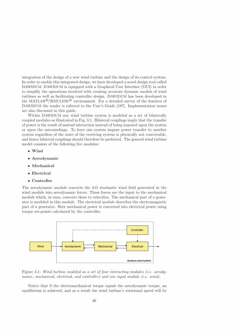
integration of the design of a new wind turbine and the design of its control system.In order to enable this integrated design, we have developed a novel design tool calledDAWIDUM. DAWIDUM is equipped with a Graphical User Interface (GUI) in orderto simplify the operations involved with creating accurate dynamic models of windturbines as well as facilitating controller design. DAWIDUM has been developed inthe MATLAB R©/SIMULINK R© environment. For a detailed survey of the features ofDAWIDUM the reader is referred to the User’s Guide [187]. Implementation issuesare also discussed in this guide.

Within DAWIDUM any wind turbine system is modeled as a set of bilaterallycoupled modules as illustrated in Fig. 3.1. Bilateral couplings imply that the transferof power is the result of mutual interaction instead of being imposed upon the systemor upon the surroundings. To have one system impose power transfer to anothersystem regardless of the state of the receiving system is physically not conceivable,and hence bilateral couplings should therefore be preferred. The general wind turbinemodel consists of the following five modules:

• Wind

• Aerodynamic

• Mechanical

• Electrical

• Controller

The aerodynamic module converts the 3-D stochastic wind field generated in thewind module into aerodynamic forces. These forces are the input to the mechanicalmodule which, in turn, converts these to velocities. The mechanical part of a gener-ator is modeled in this module. The electrical module describes the electromagneticpart of a generator. Here mechanical power is converted into electrical power usingtorque set-points calculated by the controller.

Aerodynamic ElectricalWind Mechanical

Onshore wind turbine

Controller

Figure 3.1: Wind turbine modeled as a set of four interacting modules (i.e. aerody-namic, mechanical, electrical, and controller) and one input module (i.e. wind).

Notice that if the electromechanical torque equals the aerodynamic torque, anequilibrium is achieved, and as a result the wind turbine’s rotational speed will be

46

constant. Acceleration and deceleration to new speed set-points will be achieved bydecreasing or increasing the electromechanical torque, respectively. Furthermore, ifthere are also mechanical means of controlling the aerodynamic torque, e.g. pitchcontrol (indicated by the dashed arrow in Fig. 3.1), greater operational flexibility isachieved [106]. This can be easily seen by recognizing that pitch control can nowbe used to follow minute-to-minute fluctuations in aerodynamic power, while the(almost instantaneous) torque control can focus on fatigue load reduction.

It should also be mentioned that the presented model structure can be easilyextended to being able to handle offshore wind turbines as well. The resultingmodel structure is shown in Fig. 3.2. The hydrodynamic module converts the wavefield generated in the wave module into hydrodynamic forces. It is assumed that thestructural dynamics are not influencing the wave field.

Aerodynamic ElectricalWind Mechanical

Controller

Wave

Hydrodynamic

Offshore wind turbine

Figure 3.2: Wind turbine model structure of Fig. 3.1 extended with a wave andhydrodynamic module required for offshore applications.

The division of the complete wind turbine model into modules is based on theassumption that the modules are interacting via specified interaction variables. Thiscreates a modular structure in which the user can easily exchange modules. Linkedtogether correctly the modules will describe the complete wind turbine behavior.Hence, the user can compose a specific wind turbine configuration by choosing foreach type of module (electrical, mechanical et cetera) the appropriate one out ofthe available DAWIDUM library. Moreover, any module can be modified or can bewritten totally new by the user as long as it is compatible with the presented modelstructure.

In the next sections we will discuss the main properties of the aforementionedmodules as well as the interaction variables. We start with the wind module.

47

3.2 Wind module

Wind, in the macro-meteorological sense, are movements of air masses in the at-mosphere. These large-scale movements are generated primarily by differences intemperature within the atmosphere. These temperature differences are due to theunequal heating of the crust of the earth by the sun: the equatorial regions re-ceive more solar energy than the polar regions [65]. The variations in wind velocityand direction due to atmospheric turbulence, on the other hand, form the micro-meteorological range. Consequently, the behavior and structure of the wind willvary from site to site dependent on the general climate of the region, the physicalgeography of the locality, the surface condition of the terrain around the site, andvarious other factors.

Meteorologists estimate that about 1% of the incoming solar radiation is con-verted to wind energy (≈ 1.2 · 1015 W). According to the World MeteorologicalOrganization it is possible to extract about 2 · 1013 W from the atmosphere due tolimitations in height and accessibility. Compare this figure with the world electricityconsumption (1999) of 12.8 · 1012 kWh (i.e. an average of 0.15 · 1013 W) [58].

To be able to predict the yield of wind turbines accurate information aboutthe undisturbed wind velocity Vw is essential. This knowledge is also necessary ifthe turbines are designed to withstand the imposed loads with safety and at costthat are competitive with conventional energy production (fossil or nuclear fuel)and other renewable energy sources (including biomass, photovoltaics, waterpowerand sun collectors). Combination of both results leads to the conclusion that windsimulation should be an integral part of wind turbine structural design, and analysis.

DAWIDUM’s wind module consists of two submodules, viz. “deterministic” and“stochastic”. Both contain different wind models. All models have an input-outputconfiguration as depicted in Fig. 3.3. It is assumed that neither the aerodynamics northe structural dynamics are influencing the undisturbed wind part. Consequently,the only output of this module is the undisturbed wind velocity (vector) Vw. Ob-serve that the wind vector can be a one, two or three-dimensional function of time,depending on the chosen wind model. The wind vector is described with respect tothe blade element reference frame (see Fig. 3.11 on page 58).

Figure 3.3: Wind module input-output configuration.

The deterministic submodule allows the following undisturbed wind inputs tobe specified: a uniform wind field (i.e. Vw is constant both in space and time), asequence of upward and downward stepwise changes in the wind velocity, and a userspecified WindData.mat file. The stochastic submodule is able to read the outputgenerated by SWING-4 (see Subsection 2.3.4 for detailed information about this windfield generator).

48

3.3 Aerodynamic module

This section treats the aerodynamics. DAWIDUM’s aerodynamic module has aninput-output configuration as depicted in Fig. 3.4. The only input to this module isthe undisturbed wind velocity Vw generated by the wind module. The aerodynamicmodule is bilaterally coupled to the mechanical module through the velocity vectorx (containing the blade movements with respect to the blade element referenceframe), and the aerodynamic forces Faero. In other words, the interaction betweenthe aerodynamics and the structural dynamics takes place via the blade movementsand the aerodynamic forces. This interaction is indispensable for accurate modelingof the aero-elastic behavior of, in particular, flexible wind turbines.

Figure 3.4: Aerodynamic module input-output configuration.

3.3.1 Introduction

The accurate computation of the aerodynamic forces is a very challenging prob-lem. First of all, the wind environment in which wind turbines generally operate isvariable both in space and time and has a strong stochastic content. Because thedimensions of atmospheric turbulence are of the same order as the rotor diameter,individual blades can be engulfed in coherent turbulence bells which lead to severefatigue loading that significantly can reduce the lifetime of the structure. Secondly,the blade sections can see highly variable, large angle unsteady flows at reducedfrequencies, so that non-linear and unsteady aerodynamic effects are significant. Fi-nally, the rotor blades as well as the support structure will in the (near) futurebecome more and more flexible due to the move from relatively small and rigid con-stant speed wind turbines towards increasingly lightweight and structurally flexiblewind turbines operating at variable speed.

Obviously, we need to have models that accurately describes the mutual couplingbetween the aerodynamics and the structural mechanics in order to make it possibleto identify and resolve such (aero-elastic) stability problems already in the designphase of a wind turbine. The starting point of the modeling of the aerodynamics isthe Rankine-Froude actuator-disk model which will be discussed below.

3.3.2 Rankine-Froude actuator-disk model

The simplest and oldest mathematical model which describes the wind turbine dy-namics is the Rankine-Froude actuator-disk model. The concept was introduced byR.E. Froude in 1889 [68], after W.J.M. Rankine [231] had introduced the momentumtheory. In this model the rotor is replaced by an “actuator-disk”, which is a circular

49

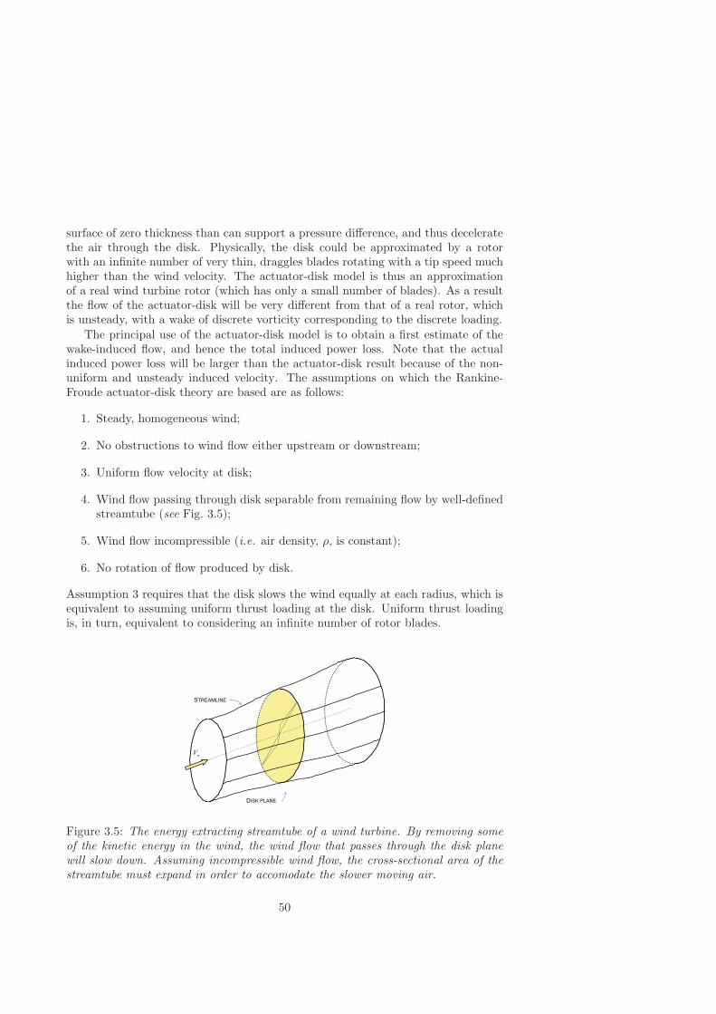
surface of zero thickness than can support a pressure difference, and thus deceleratethe air through the disk. Physically, the disk could be approximated by a rotorwith an infinite number of very thin, draggles blades rotating with a tip speed muchhigher than the wind velocity. The actuator-disk model is thus an approximationof a real wind turbine rotor (which has only a small number of blades). As a resultthe flow of the actuator-disk will be very different from that of a real rotor, whichis unsteady, with a wake of discrete vorticity corresponding to the discrete loading.

The principal use of the actuator-disk model is to obtain a first estimate of thewake-induced flow, and hence the total induced power loss. Note that the actualinduced power loss will be larger than the actuator-disk result because of the non-uniform and unsteady induced velocity. The assumptions on which the Rankine-Froude actuator-disk theory are based are as follows:

1. Steady, homogeneous wind;

2. No obstructions to wind flow either upstream or downstream;

3. Uniform flow velocity at disk;

4. Wind flow passing through disk separable from remaining flow by well-definedstreamtube (see Fig. 3.5);

5. Wind flow incompressible (i.e. air density, ρ, is constant);

6. No rotation of flow produced by disk.

Assumption 3 requires that the disk slows the wind equally at each radius, which isequivalent to assuming uniform thrust loading at the disk. Uniform thrust loadingis, in turn, equivalent to considering an infinite number of rotor blades.

Figure 3.5: The energy extracting streamtube of a wind turbine. By removing someof the kinetic energy in the wind, the wind flow that passes through the disk planewill slow down. Assuming incompressible wind flow, the cross-sectional area of thestreamtube must expand in order to accomodate the slower moving air.

50

Now consider the flow diagram of Fig. 3.6 for a cylindrical control volume ofcross-sectional area S and note sections 0, 3, 2, and 1. Let A be the area of therotor disk and ρ be the air density. Wind approaches the rotor at velocity Vw farupstream at section 0 at static pressure p0. Kinetic energy is extracted by the rotor,and the reduced velocity causes the the streamline to expand.

0p

CONTROL VOLUME

DISK PLANE

2P

3P

wV wV

SVaxV

0A

A1

A

0p

0p

0p

STREAMLINE

0 123

Figure 3.6: One-dimensional flow past the disk plane of an actuator-disk.

Fig. 3.7 shows this principle for a non-loaded and loaded machine. For instance,for a turbine with zero loading, the wind velocity in the rotor plane (Vax) is equalto the undisturbed wind velocity (Vw), while an operating and hence loaded turbineslows down the wind velocity to a lower value. If the velocity decrease induced bythe rotor is v, then the velocity at the disk is Vw − v = Vax, while far downstreamat section 1 the wind has been slowed further to velocity V∞ and the pressure hasreturned to p0. The difference between the axial component of the wind velocityand the axial flow velocity in the rotor plane is usually called the “induced” velocity,the velocity induced by the presence of the turbine.

Figure 3.7: Wind turbine with (r) and without (l) loading. Vw is the undisturbed windvelocity, Vax is the wind velocity at the rotor disk position, and V∞ is the velocity fardownstream, in the turbine wake. The unloaded wind turbine is transparent to thewind, the loaded turbine decelerates the wind. A change in loading implies a changein “induced” velocity.

51

The momentum loss of the fluid is the result of the thrust Dax that the rotorexerts against the flow, combined with the net resultant of the external pressure onthe control volume, as shown in Fig. 3.6. Since the static atmospheric pressure, p0

acts on the entire control volume, its net resultant is zero.Within the streamtube, continuity requires that VwA0 = VaxA = V∞A1. Writing

the continuity equation for flow outside the streamtube between sections 0 and 1, itfollows that there must be a net flow, Φf , out the sides of the control volume equalto the following:

Φf = Vw [(S −A0) − (S −A1)] = Vw(A1 −A0) (3.1)

Newton’s second law or equivalently law of motion can be generalized from particlesto fluids: “At any instant in steady flow the resultant force acting on the movingfluid within a fixed volume of space equals the net rate of outflow of momentum fromthe closed surface bounding that volume”. This is known as the momentum theorem.Writing the momentum theorem for the cylindrical control volume, it follows

ρV 2wS −Dax = ρV 2

w(S −A1) + ρV 2∞A1 + ρΦfVw (3.2)

Substituting Φf from Eq. (3.1) and VwA0 = V∞A1 gives the thrust as

Dax = ρA1V∞(Vw − V∞) (3.3)

To slow the wind, a force must be manifested as a pressure drop across the disk.After all, a sudden step change in velocity is not possible because of the enormousaccelerations and forces this would require. The static pressure drop just ahead thedisk is p3 and just behind the disk p2. Since it is assumed that these pressures donot vary with time, it is also assumed that there is no periodicity in the flow velocityat the rotor plane, a condition that is strictly true only for an infinite number ofblades. Applying the Bernoulli theorem from section 0 to section 3 and again fromsection 2 to section 1, we have

12ρV

2w + p0 = 1

2ρV2ax + p3 (3.4)

12ρV

2ax + p2 = 1

2ρV2∞ + p0 (3.5)

The thrust on the rotor is then

Dax = A(p3 − p2) (3.6)

Solving for the pressure difference using Eq. (3.4) and (3.5) gives

Dax = 12ρA(V 2

w − V 2∞) (3.7)

Equating Eq. (3.3) and (3.7) and using AVax = A1V∞, we find that

Vax = 12 (Vw + V∞) (3.8)

52

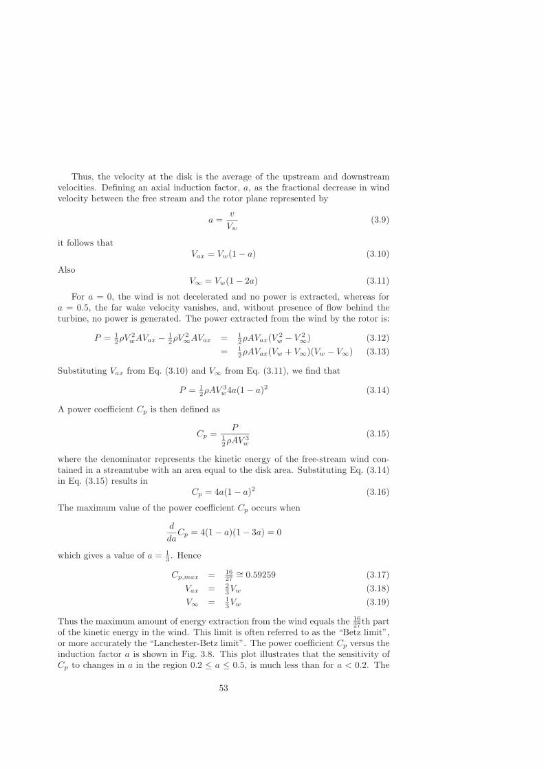
Thus, the velocity at the disk is the average of the upstream and downstreamvelocities. Defining an axial induction factor, a, as the fractional decrease in windvelocity between the free stream and the rotor plane represented by

a =v

Vw(3.9)

it follows thatVax = Vw(1 − a) (3.10)

AlsoV∞ = Vw(1 − 2a) (3.11)

For a = 0, the wind is not decelerated and no power is extracted, whereas fora = 0.5, the far wake velocity vanishes, and, without presence of flow behind theturbine, no power is generated. The power extracted from the wind by the rotor is:

P = 12ρV

2wAVax − 1

2ρV2∞AVax = 1

2ρAVax(V 2w − V 2

∞) (3.12)= 1

2ρAVax(Vw + V∞)(Vw − V∞) (3.13)

Substituting Vax from Eq. (3.10) and V∞ from Eq. (3.11), we find that

P = 12ρAV

3w4a(1 − a)2 (3.14)

A power coefficient Cp is then defined as

Cp =P

12ρAV

3w

(3.15)

where the denominator represents the kinetic energy of the free-stream wind con-tained in a streamtube with an area equal to the disk area. Substituting Eq. (3.14)in Eq. (3.15) results in

Cp = 4a(1 − a)2 (3.16)

The maximum value of the power coefficient Cp occurs when

d

daCp = 4(1 − a)(1 − 3a) = 0

which gives a value of a = 13 . Hence

Cp,max = 1627

∼= 0.59259 (3.17)Vax = 2

3Vw (3.18)V∞ = 1

3Vw (3.19)

Thus the maximum amount of energy extraction from the wind equals the 1627 th part

of the kinetic energy in the wind. This limit is often referred to as the “Betz limit”,or more accurately the “Lanchester-Betz limit”. The power coefficient Cp versus theinduction factor a is shown in Fig. 3.8. This plot illustrates that the sensitivity ofCp to changes in a in the region 0.2 ≤ a ≤ 0.5, is much less than for a < 0.2. The

53

power coefficient Cp has proved to be the most useful measure of the effectiveness ofa wind turbine [261]. The actuator disk “efficiency” ηad (i.e. power output dividedby power input), on the other hand, is

ηad =P

12ρV

2wVaxA

= 4a(1 − a) (3.20)

since the mass flow rate through the actuator disk is not ρAVw, but ρAVax orequivalently ρAVw(1 − a) using Eq. (3.10). The maximum efficiency of 1 occurs ata = 1

2 implying zero velocity in the wake (V∞ = 0) and a power coefficient of 12 . The

actuator disk efficiency is 89∼= 0.889 at the maximum power coefficient of 0.59259.

0 0.05 0.1 0.15 0.2 0.25 0.3 0.35 0.4 0.45 0.50

0.1

0.2

0.3

0.4

0.5

0.6

a [−]

Cp

[−]

Lanchester−Betz limit

Figure 3.8: Power coefficient Cp as function of the axial induction factor a. Solidline: Cp = 4a(1 − a) 2. The maximum value of Cp occurs when a = 1

3 and is equalto Cp,max = 16

27 = 0.59259.

It must be noted that according to Van Kuik [139] the radial force assumptiondoes not hold true owing to an edge singularity of the actuator disk flow, and thatthe “real” maximum of the power coefficient is to be expected to be slightly higherthan the Betz limit. Apart from this, it is possible to reach much higher powercoefficients (i.e. to by-pass the optimum of Betz) with additional devices like tipvanes [262]. These devices are all based on the concentrator and/or ejector principle.But to date almost no such devices have progressed beyond the experimental stage,mainly due to their higher complexity and expense in comparison to the free-runningturbine.

The pressure and velocity relationships of an energy extracting actuator-disk areshown in Fig. 3.9.

54

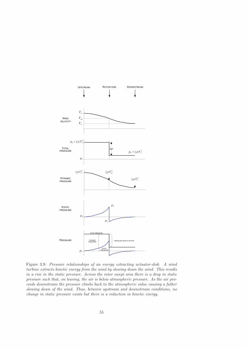
Figure 3.9: Pressure relationships of an energy extracting actuator-disk. A windturbine extracts kinetic energy from the wind by slowing down the wind. This resultsin a rise in the static pressure. Across the rotor swept area there is a drop in staticpressure such that, on leaving, the air is below atmospheric pressure. As the air pro-ceeds downstream the pressure climbs back to the atmospheric value causing a futherslowing down of the wind. Thus, between upstream and downstream conditions, nochange in static pressure exists but there is a reduction in kinetic energy.

55

The Rankine-Froude actuator-disk model has the following implications:

• The wind velocity at the rotor plane is always less than the free-stream velocitywhen power is being absorbed (i.e. Vax < Vw);

• This model assumes no wake rotation, i.e. no energy wasted in kinetic energyof a twirling wake;

• Even with the best rotor design, it is evidently not possible to extract morethan about 60 percent of the kinetic energy in the wind.

Note that the range of the axial induction factor, a, is from zero for no energyextraction to one-half, at which point the wind theoretically slows to zero velocitybehind the rotor. Outside this range, the assumptions made in deriving this modelare violated.

Additional data that can be derived from this model include the thrust loadingon the rotor. The thrust on the rotor is:

Dax = 12ρA(V 2

w − V 2∞) (3.21)

which for V∞ = Vw(1 − 2a) simplifies to

Dax = 12ρV

2wA [4a(1 − a)] = qA [4a(1 − a)] (3.22)

where q is the dynamic pressure.If we were thinking of the rotor as a propeller, we would define a thrust coefficient,

as follows:

Ct =Dax

qA(3.23)

On the other hand, if we were to think of Dax as a drag force on an equivalent flatplate of area equal to that of a rotor disk, we can define a drag coefficient, as follows:

Cdax =Dax

qA(3.24)

In either case, it is apparent from Eq. (3.16) that for these definitions

Ct = Cdax = 4a(1 − a) (3.25)

Since a flat plate has a drag coefficient of about 1.28, we can note that, for a = 13 ,

we obtain an equivalent drag coefficient of 89 for a rotor operating at the maximum

Cp condition. Thus the rotor thrust is about 30 percent less than that of a flat plateequal in diameter to the rotor. Therefore, it is easy to see that the thrust loadsgenerated by continuing to operate in high winds can be very large, requiring a verystrong rotor and tower.

56

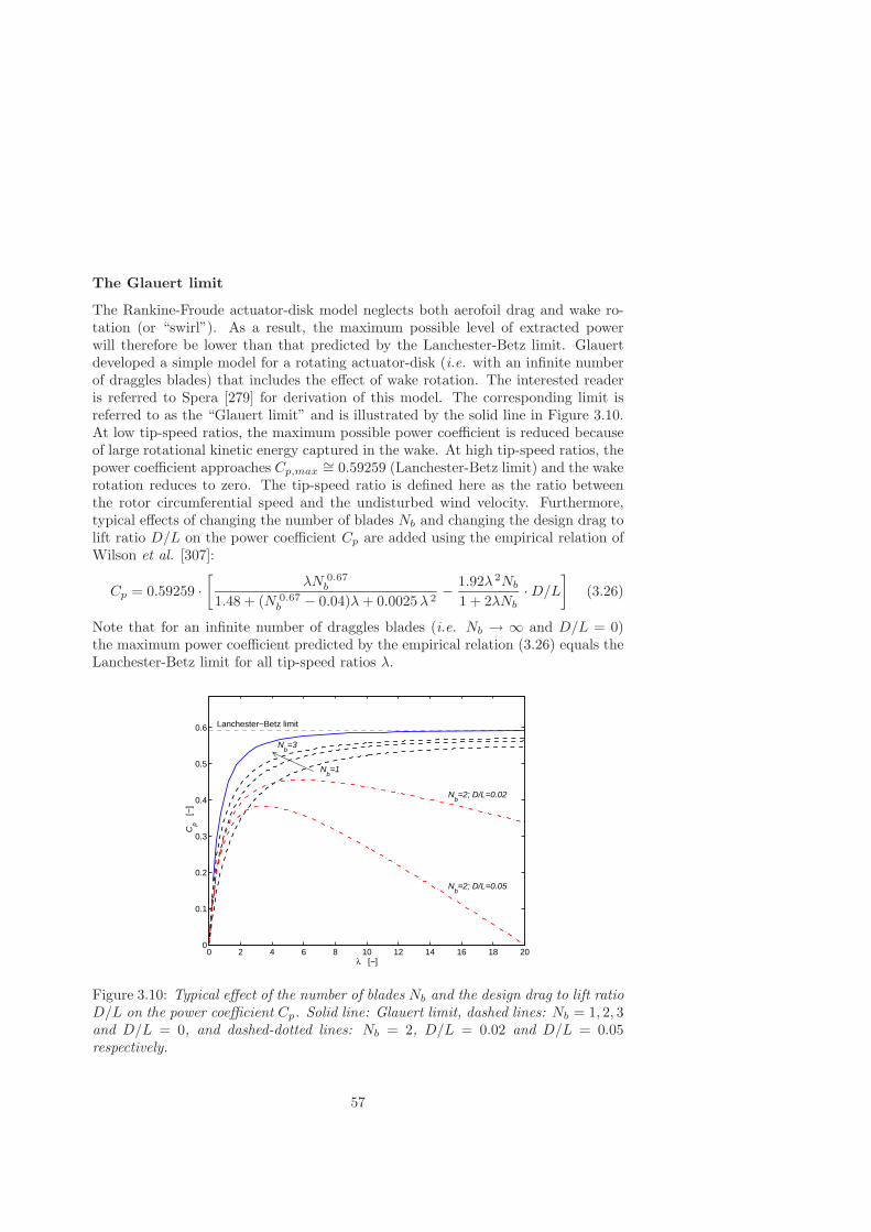
The Glauert limit

The Rankine-Froude actuator-disk model neglects both aerofoil drag and wake ro-tation (or “swirl”). As a result, the maximum possible level of extracted powerwill therefore be lower than that predicted by the Lanchester-Betz limit. Glauertdeveloped a simple model for a rotating actuator-disk (i.e. with an infinite numberof draggles blades) that includes the effect of wake rotation. The interested readeris referred to Spera [279] for derivation of this model. The corresponding limit isreferred to as the “Glauert limit” and is illustrated by the solid line in Figure 3.10.At low tip-speed ratios, the maximum possible power coefficient is reduced becauseof large rotational kinetic energy captured in the wake. At high tip-speed ratios, thepower coefficient approaches Cp,max

∼= 0.59259 (Lanchester-Betz limit) and the wakerotation reduces to zero. The tip-speed ratio is defined here as the ratio betweenthe rotor circumferential speed and the undisturbed wind velocity. Furthermore,typical effects of changing the number of blades Nb and changing the design drag tolift ratio D/L on the power coefficient Cp are added using the empirical relation ofWilson et al. [307]:

Cp = 0.59259 ·[

λN 0.67b

1.48 + (N 0.67b − 0.04)λ+ 0.0025λ 2

− 1.92λ 2Nb

1 + 2λNb·D/L

](3.26)

Note that for an infinite number of draggles blades (i.e. Nb → ∞ and D/L = 0)the maximum power coefficient predicted by the empirical relation (3.26) equals theLanchester-Betz limit for all tip-speed ratios λ.

0 2 4 6 8 10 12 14 16 18 200

0.1

0.2

0.3

0.4

0.5

0.6

λ [−]

Cp

[−]

Lanchester−Betz limit

Nb=2; D/L=0.02

Nb=2; D/L=0.05

Nb=1

Nb=3

Figure 3.10: Typical effect of the number of blades Nb and the design drag to lift ratioD/L on the power coefficient Cp. Solid line: Glauert limit, dashed lines: Nb = 1, 2, 3and D/L = 0, and dashed-dotted lines: Nb = 2, D/L = 0.02 and D/L = 0.05respectively.

57

3.3.3 Blade element momentum model

The combined blade element and momentum theory is an extension of the Rankine-Froude actuator disk theory described in Section 3.3.2. The blade element momen-tum theory divides the rotor blades into a number of radial blade sections (elements),each at a particular angle of attack. These blade elements are assumed to have thesame aerodynamic properties as an infinitely long (or 2-D) rotor blade with the samechord, and aerofoils. This implies that 2-D aerofoil data (i.e. lift, drag and momentcoefficients) obtained from wind tunnel experiments may be used. The airflow fromupstream to downstream of the elements is, in turn, divided into annular streamtubes. It is assumed that each stream tube can be treated independently from ad-jacent ones. Subsequently, the theory outlined in the preceding section is applied toeach blade element, instead of to the rotor disk as a whole. The velocity componentin the span-wise direction (i.e. perpendicular to the blade cross-section) is ignored.Finally, the total load is calculated by adding up the forces from all the elements.

The contribution of each blade element to the lift and drag force can be derivedas follows. Consider an annular cross-section of a rotor blade as depicted in Fig. 3.11,and examine an element of length ∆r of one blade.

Figure 3.11: Blade element velocities, and aerodynamic forces w.r.t the blade localcoordinate frame with the chord line as reference.

58

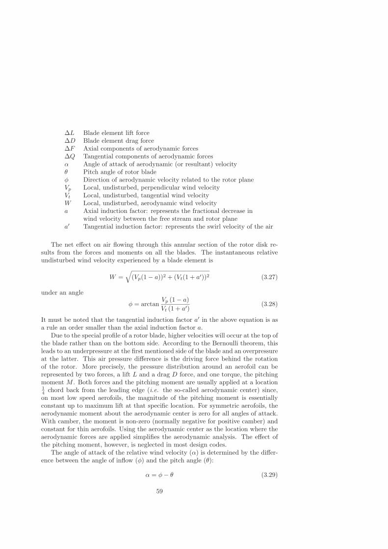
∆L Blade element lift force∆D Blade element drag force∆F Axial components of aerodynamic forces∆Q Tangential components of aerodynamic forcesα Angle of attack of aerodynamic (or resultant) velocityθ Pitch angle of rotor bladeφ Direction of aerodynamic velocity related to the rotor planeVp Local, undisturbed, perpendicular wind velocityVt Local, undisturbed, tangential wind velocityW Local, undisturbed, aerodynamic wind velocitya Axial induction factor: represents the fractional decrease in

wind velocity between the free stream and rotor planea′ Tangential induction factor: represents the swirl velocity of the air

The net effect on air flowing through this annular section of the rotor disk re-sults from the forces and moments on all the blades. The instantaneous relativeundisturbed wind velocity experienced by a blade element is

W =√

(Vp(1 − a))2 + (Vt(1 + a′))2 (3.27)

under an angle

φ = arctanVp (1 − a)Vt (1 + a′)

(3.28)

It must be noted that the tangential induction factor a′ in the above equation is asa rule an order smaller than the axial induction factor a.

Due to the special profile of a rotor blade, higher velocities will occur at the top ofthe blade rather than on the bottom side. According to the Bernoulli theorem, thisleads to an underpressure at the first mentioned side of the blade and an overpressureat the latter. This air pressure difference is the driving force behind the rotationof the rotor. More precisely, the pressure distribution around an aerofoil can berepresented by two forces, a lift L and a drag D force, and one torque, the pitchingmoment M . Both forces and the pitching moment are usually applied at a location14 chord back from the leading edge (i.e. the so-called aerodynamic center) since,on most low speed aerofoils, the magnitude of the pitching moment is essentiallyconstant up to maximum lift at that specific location. For symmetric aerofoils, theaerodynamic moment about the aerodynamic center is zero for all angles of attack.With camber, the moment is non-zero (normally negative for positive camber) andconstant for thin aerofoils. Using the aerodynamic center as the location where theaerodynamic forces are applied simplifies the aerodynamic analysis. The effect ofthe pitching moment, however, is neglected in most design codes.

The angle of attack of the relative wind velocity (α) is determined by the differ-ence between the angle of inflow (φ) and the pitch angle (θ):

α = φ− θ (3.29)

59

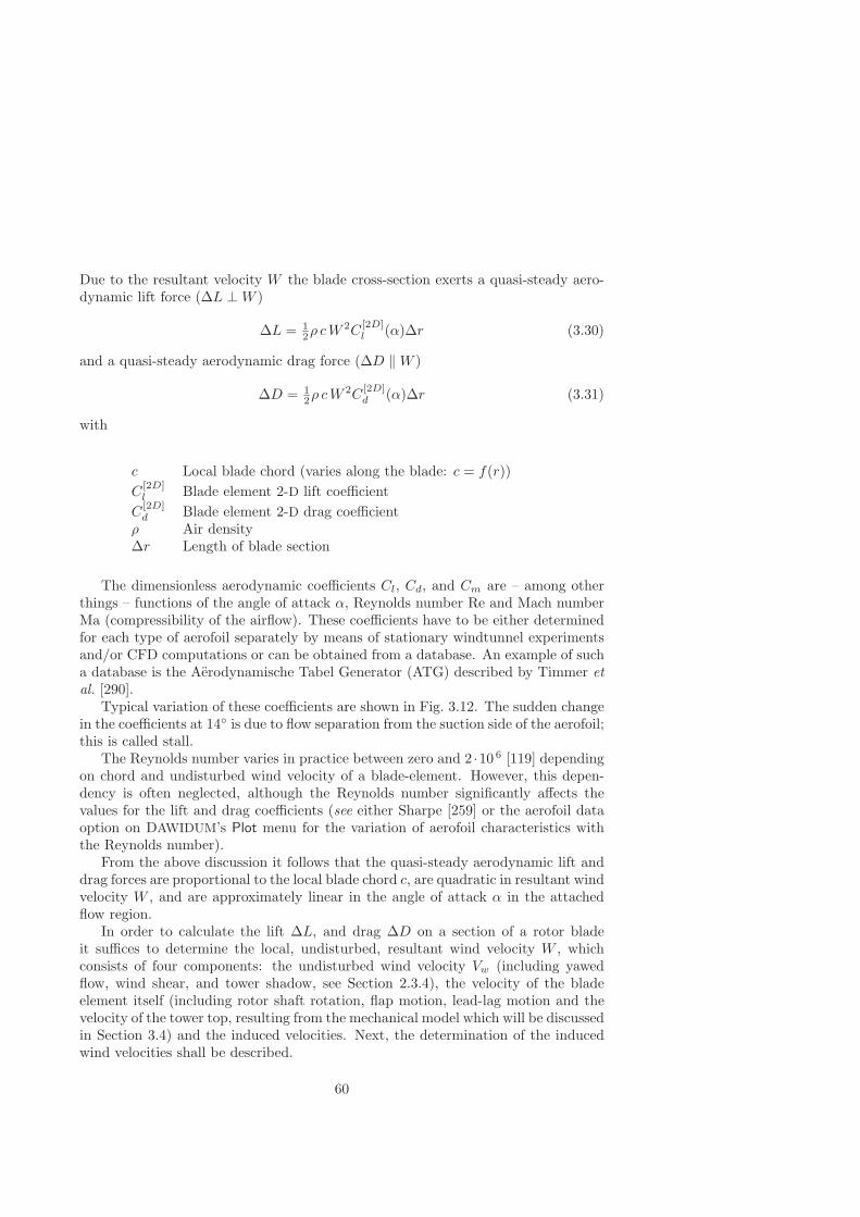
Due to the resultant velocity W the blade cross-section exerts a quasi-steady aero-dynamic lift force (∆L ⊥W )

∆L = 12ρ cW

2C[2D]l (α)∆r (3.30)

and a quasi-steady aerodynamic drag force (∆D ‖W )

∆D = 12ρ cW

2C[2D]d (α)∆r (3.31)

with

c Local blade chord (varies along the blade: c = f(r))C

[2D]l Blade element 2-D lift coefficient

C[2D]d Blade element 2-D drag coefficient

ρ Air density∆r Length of blade section

The dimensionless aerodynamic coefficients Cl, Cd, and Cm are – among otherthings – functions of the angle of attack α, Reynolds number Re and Mach numberMa (compressibility of the airflow). These coefficients have to be either determinedfor each type of aerofoil separately by means of stationary windtunnel experimentsand/or CFD computations or can be obtained from a database. An example of sucha database is the Aerodynamische Tabel Generator (ATG) described by Timmer etal. [290].

Typical variation of these coefficients are shown in Fig. 3.12. The sudden changein the coefficients at 14 is due to flow separation from the suction side of the aerofoil;this is called stall.

The Reynolds number varies in practice between zero and 2 ·10 6 [119] dependingon chord and undisturbed wind velocity of a blade-element. However, this depen-dency is often neglected, although the Reynolds number significantly affects thevalues for the lift and drag coefficients (see either Sharpe [259] or the aerofoil dataoption on DAWIDUM’s Plot menu for the variation of aerofoil characteristics withthe Reynolds number).

From the above discussion it follows that the quasi-steady aerodynamic lift anddrag forces are proportional to the local blade chord c, are quadratic in resultant windvelocity W , and are approximately linear in the angle of attack α in the attachedflow region.

In order to calculate the lift ∆L, and drag ∆D on a section of a rotor bladeit suffices to determine the local, undisturbed, resultant wind velocity W , whichconsists of four components: the undisturbed wind velocity Vw (including yawedflow, wind shear, and tower shadow, see Section 2.3.4), the velocity of the bladeelement itself (including rotor shaft rotation, flap motion, lead-lag motion and thevelocity of the tower top, resulting from the mechanical model which will be discussedin Section 3.4) and the induced velocities. Next, the determination of the inducedwind velocities shall be described.

60

−10 0 10 20 30 40 50 60 70 80 90

−0.5

0

0.5

1

1.5

α [deg]

Cl

Cd

Cm

Stalled flowAttached flow

Cl ,

Cd ,

and

Cm

[−

]

→←← →

Figure 3.12: Typical variation of the 2-D lift, drag, and moment coefficient as func-tion of the angle of attack α. Solid curve: lift coefficient Cl, dashed curve: dragcoefficient Cd, and dashed-dotted curve: moment coefficient Cm about the aerody-namic center.

Induced velocities

In the equilibrium situation, the axial flow in the rotor plane of a wind turbine,depends on the wind velocity, and on the degree of loading (i.e. the size of axialforce Dax =

∑∆F ) of the turbine. For instance, for a turbine with zero loading,

the wind velocity at the rotor disk position (Vax) is equal to the undisturbed windvelocity (Vw), while an operating, and hence loaded turbine slows down the windvelocity to a lower value (see Fig. 3.7 on page 51). The difference between the axialcomponent of the wind velocity and the axial flow velocity in the rotor plane isusually called the “axial induced” velocity, the velocity induced by the presence ofthe turbine. The tangential flow, on the other hand, is induced by the swirl velocityof the air flow around the blade.

Horizontal-axis wind turbine rotors are usually not aligned with the wind dueto the continuously changing wind direction and the fact that no rotor is capable offollowing this variability. Furthermore, upwind rotors are sometimes tilted in orderto increase the tower clearance, and hence to reduce tower shadow. In effect, therotor is then yawed about a horizontal axis. For all these reasons it is thus necessaryto include in the blade element momentum theory the effects of yaw. Here we willconsider only the simple case of perpendicular flow.

The axial induced velocity can be determined by expressing the axial thrust ∆Fon a blade element either as the rate of change of momentum in the annular ringswept out by this element

∆F = 4ρπrV 2p a(1 − a)∆r (3.32)

61

using Eq. (3.22) with A π(r + 12∆r)2 − π(r − 1

2∆r)2 = 2πr∆r the area of theannular ring, or as the force exerted by the wind on a blade element

∆F = Nb(∆L cosφ+ ∆D sinφ)= 1

2ρW2Nb c

(C 2D

l cosφ+ C 2Dd sinφ

)︸ ︷︷ ︸CN

∆r (3.33)

where Nb is the number of rotor blades. Assuming equality of Eqs. (3.32) and (3.33)gives

4a(1 − a) =W 2Nb c (C 2D

l cosφ+ C 2Dd sinφ)

2πrV 2p︸ ︷︷ ︸

Cdax

(3.34)

The right-hand side term is defined as the dimensionless thrust coefficient Cdax (seeEq. (3.25)). Solving the above equation gives

4a(1 − a) = Cdax

⇒ a = 12 − 1

2

√1 − Cdax (3.35)

as an expression for the axial induction factor in case of perpendicular flow. Alter-natively, the axial induction factor can be calculated as

a =σrCN

4 sin2(φ) + σrCN

(3.36)

by substituting

CN = C 2Dl cosφ+ C 2D

d sinφ

sin(φ) =Vp (1 − a)

W

σr =Nb c

2πr

in Eq. (3.34) and solving for a. The term σr (which is a function of the radius r) iscalled the local solidity or chord solidity.

The tangential induced velocity can, on the other hand, be determined by ex-pressing the torque ∆Q on a blade element either as the rate of change of angularmomentum

∆Q = 4ρπr∆r(1 − a)VpVt ra′ (3.37)

or as the torque exerted by the wind on a blade element

∆Q = Nb(∆L sinφ− ∆D cosφ)r= 1

2ρW2Nb c (C 2D

l sinφ− C 2Dd cosφ)︸ ︷︷ ︸

CT

r∆r (3.38)

62

assuming Nb blades. Again assuming equality between the above expressions of thetorque on a blade element we have

a′ =W 2Nb c (C 2D

l sinφ− C 2Dd cosφ)

8πVtVp r(1 − a)(3.39)

as an expression for the tangential induction factor. Alternatively, the tangentialinduction factor can be calculated as

a′ =σrCT

4 sin(φ) cos(φ) − σrCT(3.40)

withCT = C 2D

l sinφ− C 2Dd cosφ

and

sin(φ) =Vp (1 − a)

W

cos(φ) =Vt (1 + a′)

W

σr =Nb c

2πr

Thus, Eqs. (3.35)/(3.36) and (3.39)/(3.40) are the set of non-linear relations thatdetermine the dimensionless induced velocities a, and a′ in case of perpendicularflow. Before these equations can be used, however, the local thrust coefficient mustbe modified to account for two effects: the departure of the local thrust coefficientfrom the momentum relation, and the non-uniformity of the induced velocities inthe flow. These so-called tip losses will be considered after the treatment of theturbulent wake state.

Turbulent wake state

For heavily loaded wind turbines, which implies a high axial induction factor a aswell as a high tangential induction factor a′, the momentum and vortex theory areno longer applicable because of the predicted reversal of flow in the turbine wake.The vortex structure disintegrates and the wake becomes turbulent and, in doingso, entrains energetic air from outside the wake by a mixing process. Thereby thusaltering the mass flow rate from that flowing through the actuator disk. The turbineis now operating in the so-called “turbulent wake state”, which is an intermediatestate between windmill, and propellor state (see Appendix B for an overview of thedifferent flow states of a wind turbine rotor).

In the turbulent wake state the relationship between the axial induction factorand the thrust coefficient according to the momentum theory, Eq. (3.35), has to bereplaced by an empirical relation. The explanation for this is that the momentumtheory predicts a decreasing thrust coefficient with an increasing axial induction

63

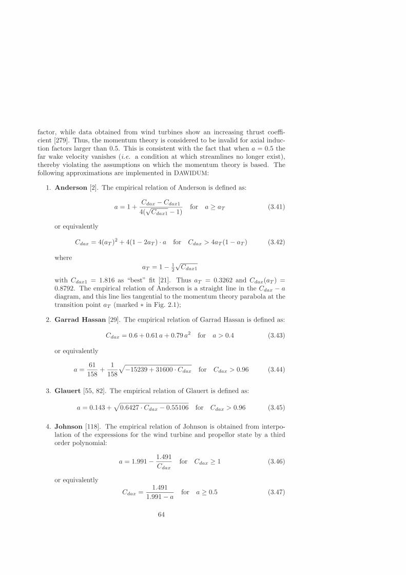
factor, while data obtained from wind turbines show an increasing thrust coeffi-cient [279]. Thus, the momentum theory is considered to be invalid for axial induc-tion factors larger than 0.5. This is consistent with the fact that when a = 0.5 thefar wake velocity vanishes (i.e. a condition at which streamlines no longer exist),thereby violating the assumptions on which the momentum theory is based. Thefollowing approximations are implemented in DAWIDUM:

1. Anderson [2]. The empirical relation of Anderson is defined as:

a = 1 +Cdax − Cdax1

4(√Cdax1 − 1)

for a ≥ aT (3.41)

or equivalently

Cdax = 4(aT )2 + 4(1 − 2aT ) · a for Cdax > 4aT (1 − aT ) (3.42)

whereaT = 1 − 1

2

√Cdax1

with Cdax1 = 1.816 as “best” fit [21]. Thus aT = 0.3262 and Cdax(aT ) =0.8792. The empirical relation of Anderson is a straight line in the Cdax − adiagram, and this line lies tangential to the momentum theory parabola at thetransition point aT (marked ∗ in Fig. 2.1);

2. Garrad Hassan [29]. The empirical relation of Garrad Hassan is defined as:

Cdax = 0.6 + 0.61 a+ 0.79 a2 for a > 0.4 (3.43)

or equivalently

a =61158

+1

158

√−15239 + 31600 · Cdax for Cdax > 0.96 (3.44)

3. Glauert [55, 82]. The empirical relation of Glauert is defined as:

a = 0.143 +√

0.6427 · Cdax − 0.55106 for Cdax > 0.96 (3.45)

4. Johnson [118]. The empirical relation of Johnson is obtained from interpo-lation of the expressions for the wind turbine and propellor state by a thirdorder polynomial:

a = 1.991 − 1.491Cdax

for Cdax ≥ 1 (3.46)

or equivalently

Cdax =1.491

1.991 − afor a ≥ 0.5 (3.47)

64

5. Wilson [280, 308]. The empirical relation of Wilson is defined as:

Cdax = 4[a 2

c + (1 − 2ac)a]

for a > ac (3.48)

or equivalently

a = 14 · Cdax − 4a 2

c

1 − 2acfor Cdax > 4ac(1 − ac) (3.49)

whereac ≈ 0.2

This is a linear extrapolation of the from the momentum theory parabola atthe transition point aC (marked o in Fig. 2.1);

Observe that the empirical relation of Wilson is identical to that of Anderson, onlythe location of the transition point is different. The five mentioned approximationswere already compared in Fig. 2.1 on page 25 for perpendicular flow. From theobserved differences it has been concluded that the listed empirical approximationsmust be regarded as being only approximate at best. The prediction is, nevertheless,more realistic than the one from the momentum theory as illustrated in Fig. B.1 onpage 228. It must be noted that, in general, the value of the axial induction factorrarely exceeds 0.6 and for a well-designed blade it will be in the vicinity of 0.33 formuch of its operating range [37].

Thus for values of Cdax greater than the (empirical model dependent) transitionpoint, the right-hand side term of Eq. (3.34) needs to be substituted in one of theabove mentioned empirical relations (i.e. either Eq. (3.41), (3.44), (3.45), (3.46), or(3.49)) to compute a.

Blade tip and root effects

The blade momentum theory, as previously developed, does not account for theeffect of a finite number of rotor blades. Therefore a correction has to be applied forthe interaction of the shed vorticity with the blade’s bound vorticity. This effect isusually greatest near the blade tip, and it significantly affects the rotor torque andthrust.

Either an approximate solution by Prandtl or a more exact solution by Goldsteincan be used to account for the non-uniformity of the induced axial velocity [55]. Bothapproximations give similar results. The expression obtained by Prandtl is howevercommonly used, since this has a simple closed form, whereas the Goldstein solutionis represented by an infinite series of modified Bessel functions.

This expression is in literature denoted with the misleading term tip-loss factor.Misleading because it corrects for the fact that induction is not uniform over theannulus under consideration owing to the finite number of blades, and not for thefiniteness of the blades. Prandtl’s tip-loss factor is defined as

Ftip =2π

arccos e−(R−ri)Nb2ri sin φi (3.50)

65

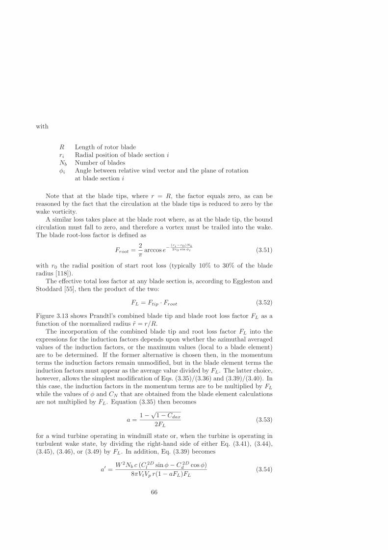
with

R Length of rotor bladeri Radial position of blade section iNb Number of bladesφi Angle between relative wind vector and the plane of rotation

at blade section i

Note that at the blade tips, where r = R, the factor equals zero, as can bereasoned by the fact that the circulation at the blade tips is reduced to zero by thewake vorticity.

A similar loss takes place at the blade root where, as at the blade tip, the boundcirculation must fall to zero, and therefore a vortex must be trailed into the wake.The blade root-loss factor is defined as

Froot =2π

arccos e−(ri−r0)Nb2r0 sin φi (3.51)

with r0 the radial position of start root loss (typically 10% to 30% of the bladeradius [118]).

The effective total loss factor at any blade section is, according to Eggleston andStoddard [55], then the product of the two:

FL = Ftip · Froot (3.52)

Figure 3.13 shows Prandtl’s combined blade tip and blade root loss factor FL as afunction of the normalized radius r = r/R.

The incorporation of the combined blade tip and root loss factor FL into theexpressions for the induction factors depends upon whether the azimuthal averagedvalues of the induction factors, or the maximum values (local to a blade element)are to be determined. If the former alternative is chosen then, in the momentumterms the induction factors remain unmodified, but in the blade element terms theinduction factors must appear as the average value divided by FL. The latter choice,however, allows the simplest modification of Eqs. (3.35)/(3.36) and (3.39)/(3.40). Inthis case, the induction factors in the momentum terms are to be multiplied by FL

while the values of φ and CN that are obtained from the blade element calculationsare not multiplied by FL. Equation (3.35) then becomes

a =1 −√

1 − Cdax

2FL(3.53)

for a wind turbine operating in windmill state or, when the turbine is operating inturbulent wake state, by dividing the right-hand side of either Eq. (3.41), (3.44),(3.45), (3.46), or (3.49) by FL. In addition, Eq. (3.39) becomes

a′ =W 2Nb c (C 2D

l sinφ− C 2Dd cosφ)

8πVtVp r(1 − aFL)FL(3.54)

66

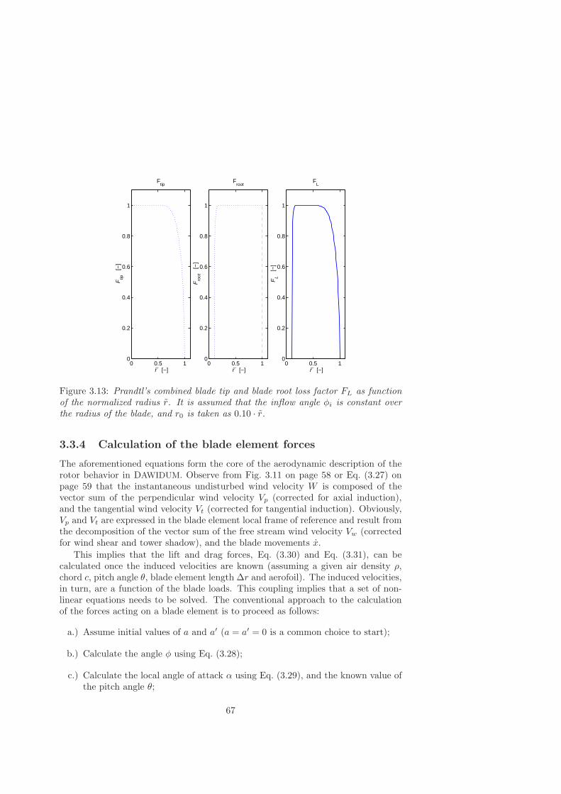
0 0.5 10

0.2

0.4

0.6

0.8

1

r [−]

Ftip

[−

]

∼

Ftip

0 0.5 10

0.2

0.4

0.6

0.8

1

r [−]

Fro

ot

[−]

∼

Froot

0 0.5 10

0.2

0.4

0.6

0.8

1

r [−]

FL

[−]

∼

FL

Figure 3.13: Prandtl’s combined blade tip and blade root loss factor FL as functionof the normalized radius r. It is assumed that the inflow angle φi is constant overthe radius of the blade, and r0 is taken as 0.10 · r.

3.3.4 Calculation of the blade element forces

The aforementioned equations form the core of the aerodynamic description of therotor behavior in DAWIDUM. Observe from Fig. 3.11 on page 58 or Eq. (3.27) onpage 59 that the instantaneous undisturbed wind velocity W is composed of thevector sum of the perpendicular wind velocity Vp (corrected for axial induction),and the tangential wind velocity Vt (corrected for tangential induction). Obviously,Vp and Vt are expressed in the blade element local frame of reference and result fromthe decomposition of the vector sum of the free stream wind velocity Vw (correctedfor wind shear and tower shadow), and the blade movements x.

This implies that the lift and drag forces, Eq. (3.30) and Eq. (3.31), can becalculated once the induced velocities are known (assuming a given air density ρ,chord c, pitch angle θ, blade element length ∆r and aerofoil). The induced velocities,in turn, are a function of the blade loads. This coupling implies that a set of non-linear equations needs to be solved. The conventional approach to the calculationof the forces acting on a blade element is to proceed as follows:

a.) Assume initial values of a and a′ (a = a′ = 0 is a common choice to start);

b.) Calculate the angle φ using Eq. (3.28);

c.) Calculate the local angle of attack α using Eq. (3.29), and the known value ofthe pitch angle θ;

67

d.) Determine the lift coefficient Cl and drag coefficient Cd by substituting thecalculated values for α in a look-up table containing both Cl(α) and Cd(α) ofthe aerodynamic profile for the correct Reynolds number;

e.) Calculate total loss factor FL using Eq. (3.52);

f.) Calculate Cdax using right-hand side term of Eq. (3.34) and determine in whichflow state the turbine is operating;

g.) Calculate a new value of a using either Eq. (3.53) (windmill state) or usingone of the empirical relations divided by FL (either Eq. (3.41), (3.44), (3.45),(3.46), or (3.49)) in case the turbine is operating in turbulent wake state;

h.) Calculate a new value of a′ using Eq. (3.54);

i.) Incrementally adapt a and a′ and repeat steps b.) to h.) until convergenceoccurs (difference between two successive estimates of a and a′ is smaller thanthe prescribed tolerance) or for a specified maximum number of iterations.

Once the iterations have converged, the blade element forces can be computed foreach blade as follows:

∆Fp = 12ρW

2 c(C 2D

l cosφ+ C 2Dd sinφ

)∆r (3.55)

∆Ft = 12ρW

2 c(C 2D

l sinφ− C 2Dd cosφ

)∆r (3.56)

with Fp ‖ Vp and Ft ‖ Vt. These forces are input to the mechanical module describingthe structural dynamics. This module is discussed in the next section. Finally, thenext time step can be computed.

Within DAWIDUM, the adaptation is performed by minimization of the followingobjective function

Fobj = (a− aold)2 + (a′ − a′old)

2

using the Nelder and Mead Simplex method [199]. This is a direct search methodthat does not use numerical or analytic gradients. The interested reader is referredto Chapter 5 for a detailed treatment of this method. The aerodynamic moduleis coded as an M-File S-Function1 named BEM. In this S-Function, deterministiceffects as wind shear, tower shadow and the ten-minute average wind speed at hubheight are added to the zero-mean stochastic components of SWING-4 before theforces are computed.

Up to now, the selection of the number of blade elements Ns has not beendealt with. A common choice is to select Ns from the range 10 < Ns < 20. Theactual number of blade elements, however, depends on various factors, including thefollowing ones:

• chord variation over the rotor blade;

• number of aerodynamic profiles per blade;1An M-File S-Function is a computer language description of a SIMULINK block written in

MATLAB.

68

• number of rigid bodies used to model the structural dynamics.

At present, an optimization procedure that calculates the minimum number of bladeelements for a given wind turbine configuration is not available. Within DAWIDUM

the number of blade elements can be changed easily to evaluate the effect this numberhas on the performance. Moreover, the number can be chosen independently of thenumber of rigid bodies the flexible rotor blade has been subdivided in.

One last point about the BEM theory. The basic assumption is that the forceacting on a blade element is solely responsible for the change of momentum of theair which passes through the annulus swept by that element. It is therefore assumedthat there is no radial interaction between adjacent annuli. This condition is, strictly,only true if the axial induction factor does not vary radially. The axial inductionfactor, however, varies not only radially, but also azimuthally due to various reasons(including unsteady wind and yawed flow). The question remains: is it legitimateto apply the BEM theory for the cost-effective design and operation of a flexiblewind turbines operating in turbulent wind? At present, neither an affirmative ora negative answer can be given. It is strongly recommended to perform validationexperiments in order to reveal whether it is satisfactory to use this approach todetermine the forces acting on each blade (element).

3.4 Mechanical module

In this section a systematic procedure for modeling the structural dynamics of flexi-ble wind turbines is developed. The mechanical module has an input-output config-uration as depicted in Fig. 3.14. This module is bilaterally coupled to the aerody-namic module through the velocity x, and the aerodynamic forces Faero = [Fp,1(1 :Ns) Ft,1(1 : Ns) · · ·Fp,Nb

(1 : Ns) Ft,Nb(1 : Ns)] (with Ns the number of blade ele-

ments and Nb the number of rotor blades), and is bilaterally coupled to the electricalmodule through the mechanical speed ωm, and the electromechanical torque Tem.

Figure 3.14: Mechanical module input-output configuration with the interaction vari-ables.

3.4.1 Introduction

At present, four different kinds of mechanical models are commonly used to model(flexible) mechanical structures: Finite Element (FES), Multibody (MBS), Contin-uous, and Hybrid Multibody systems (HMBS) [190]. The complexity of the me-chanical models increases in the mentioned order. Without exception, all differentkinds of mechanical models are based on the classical mechanics formulated by Sir

69

Isaac Newton (1642-1727) in his book Philosophiæ Naturalis Principia Mathematicain 1687 [200].

The general guideline in mechanical modeling always should be: devise a modelas simple as possible. It is the combination of theoretical knowledge, and practicalexperience which leads to models well suited for the intended use. Due to theextensiveness of the subject and the wide range of literature on this topic, a numberof aspects of the mentioned mechanical models will be reviewed in bird’s-eye view.

In the FES method, a real flexible structure is regarded as an assembly of afinite, but large number of geometrically simple, discrete elements. In general, thenumber of elements varies between a hundred and some thousands. Each elementconsists of a number of nodes (ranging from 2 to 27 nodes per element) with 1 to12 degrees of freedom at each node [176]. Models based on this method have thusmany degrees of freedom, with the associated high computational cost. Finite Ele-ment models are appropriate for the analysis of static loads, small dynamic motionsreferred to an inertial system, and may be very useful for layout and design, becausestress calculations give important hints for design and dimensioning of the structuralelements [140]. These models are, however, not suitable for control system design ifnot combined with an order reduction.

In the Multibody System (MBS) approach, a real mechanical system is approx-imated with a finite number of rigid bodies, coupled by inelastic joints (e.g. slider,pin) to the Newtonian reference frame. Consequently, such a system can be de-scribed with a finite number of differential equations. The essential dynamics of stiffmechanical systems that undergo large displacements as well as large rotations canbe well reproduced in this way. However, when the deformation of (a part of) thesystem has a significant effect on the dynamic behavior, the elasticity can no longerbe neglected. Inclusion of elasticity by so-called flexible bodies is essential in orderto reach the level of accuracy of stiff mechanical systems. The price to be paid is, ofcourse, an increased model order. Since the number of equations of motion remainscomparatively small, this approach is very appropriate for control system design.

A Continuous System (COS) consists of flexible bodies of which the distribu-tion of mass and stiffness can be exactly mathematically represented. The resultingset of partial differential equations (PDE’s) can be solved exactly only in a fewsimple cases. An example of a continuous system is an Euler-Bernoulli beam ofwhich the exact solution is given in Section 4.2. Due to this limitation, approximatefinite-dimensional equations of motion are normally used [128]. Moreover, the de-scription of the dynamics by partial differential equations is not suited for controldesign [21]. In the most common approximation technique, a spatial discretizationis used, whereby the partial differential equations are replaced by ordinary differen-tial equations (ODE’s). Note that while spatial discretization is used, the resultingordinary differential equations are still continuous with respect to time. Time dis-cretization can also be used, of course, and the resulting equations would be of thedifference type. The two most common spatial discretization methods are the as-sumed modes, and the finite element method respectively. Both approaches leadto linear, finite dimensional, continuous time equations of motion for approxima-tion the dynamics of flexible systems. Remark: the widely adopted term “assumed

70

modes” is sometimes confusing, because the real system normal modes of vibrationare approximated by a linear combination of the assumed modes.

A Hybrid Multibody System (HMBS) may be built up of a combination off allthree methods of modeling mentioned above, leading to the most complex model ofa mechanical system.

An overview of the main features of the four modeling concepts is given in Ta-ble 3.1. From this table it can be concluded that many physical systems of interest,and of practical importance can be effectively modeled as multibody systems. “Effec-tively” means that this approach results in a limited order model of the real systemunder consideration. In addition, the model parameters have a clear physical in-terpretation (i.e. are related to geometry and material properties). Such a modelis well suited for time-domain simulation, analysis of dynamic loads, and controlsystem design. The COS mechanical modeling method, on the other hand, can onlybe applied to very simple geometric structures (e.g. beams). The Finite Elementapproach results in complex, high order models mainly suited for layout, design, andthorough system analysis.

Mechanical modeling concepts

Modeling HMBSMBS COS FES

Body rigid and/or flexible flexible flexible

Geometry complex simple complex

Deflections large non-linear large non-linear small linearand/or small linear and/or non-linear

Description of reduced available availabledeformation

Forces/moments discrete smoothly discretedistributed

Suitability for time- good poor poordomain simulation

Suitability for control good after reduction conditional,system design after reduction

Table 3.1: Overview of the four modeling variants, with MBS: Multibody System,COS: Continuous System, FES: Finite Element System, and HMBS: Hybrid Multi-body System.

71

Based on these conclusions, we have chosen the multibody approach to be mostsuited for our goal. There are several ways of modeling flexible bodies within theMBS methodology, for an overview see e.g. Shabana [257, 258]. The simplest wayis to equally distribute the mass of the flexible body into lumped masses, intercon-nected by ideal, massless springs and dampers. This is the so-called “lumped-massmethod”. A more accurate model is obtained by using the concept of the so-called“superelement” as introduced by Rauh and Schiehlen [232, 233]. The interestedreader is referred to Appendix C where the exact calculated eigenfrequencies of anEuler-Bernoulli beam are compared with those of the finite element, lumped-massand the superelement method.

3.4.2 Superelement approach

In the superelement approach, a (part of a) flexible body is approximated with anumber of so-called superelements. Each symmetric superelement consists of 3 rigidbodies connected by joints (marked in Fig. 3.15) containing ideal torsional springsthat model the elastic properties in bending direction. The attractive feature ofmodeling the flexibility by joint springs and dampers is that the spring and damperforces are readily incorporated into the standard (rigid) multibody body packages(e.g. SD/FAST R© [109]).

It should be noted that the centre body of a superelement can be divided in twoparts of equal length to include axial deflection, and torsion deformation as well.In this thesis we limit ourselves (initially) to bending since the first torsional modeand the first two (non-rotating) bending modes of the Lagerwey LW-50/750 windturbine are sufficient apart (see Table A.2 on page 223). That is, for the LagerweyLW-50/750 wind turbine it is not necessary to take the torsional mode of vibrationinto account.

M

F

2

2zc

1zc

3zc

y

x

1

Figure 3.15: Deflections and slopes of a superelement with bending stifness EI, andlength L. Each (symmetric) superelement consists of three rigid bodies (with lengthskL, (1 − 2k)L, and kL) connected by joints ().

The main question is “What should the values of the spring constants be inorder to produce a comprehensive and accurate dynamic model of a flexible body?”

72

Accurate in the sense that i) the elastic deformations of the superelement under astatic load should be equal to those of a flexible beam, ii) the superelement shouldhave the same mass and inertia properties as a rigid beam with identical dimensions,and iii) the eigenfrequencies of the superelement should be as close as possible tothose of a continuous beam. Next, we will derive the spring constants in bendingdirection required in the superelement approach. The interested reader is referred toMolenaar [189] for the determination of the spring constants representing the axialdeflection and the torsion deformation.

Continuous bending expressions

If it is assumed that both the shear deformation and rotational inertia of the flexiblebody cross-sections are negligible if compared with bending deformation and trans-lational inertia, the spring constants can be derived from the differential equationof the deflection curve of a prismatic beam (i.e. beam with constant cross sectionthroughout its length). This equation is given in Gere & Timoshenko [76] as

d 2v

dy2= −M

EI(3.57)

with

v Transverse displacement (v ⊥ y) [m]y Distance from the origin [m]M Bending moment [Nm]E Modulus of elasticity [Pa]I Area moment of inertia [m4]

It should be noted that Eq. (3.57) is valid only when Hooke’s law applies for thematerial, and when the slope of the deflection curve is very small. Also, since effectsof shear deformations are disregarded, the equation describes only deformations dueto pure bending.

For a tapered beam, the presented relationship gives satisfactory results providedthat the angle of taper is small (i.e. < 10). In that case, Eq. (3.57) has to be writtenin the following form

d 2v

dy2= − M

EI(y)(3.58)

in which I(y) is the area moment of inertia of the cross-section at distance y fromthe origin.

Determination parameters superelement

The superelement parameters (i.e. the torsional spring constants cz1, cz2, and cz3

see Fig. 3.15) are found by comparing the deflection and the angle of rotation at

73

the free end of a Euler-Bernoulli beam (i.e. a prismatic beam with length L, cross-section area A, constant flexural rigidity EIz, and uniformly distributed mass perunit length ρ = m/L, where m is the total mass of the beam) subjected to a loadF and couple M at the free end of the beam (see Fig. 3.16). Since this is a caseof pure bending, we may use Eq. (3.57) to determine the total deflection δ and thetotal angle of rotation θ at the free end [76].

Substituting the expression for the bending moment, the differential equationbecomes

EIzv′′ = −M = FL− Fy

with v′′ = d 2vdy2 . The first integration of this equation gives

EIzv′ = FLy − Fy2

2+ C1

The constant of integration C1 can be found from the condition that the slope ofthe beam is zero at the support; thus v′(0) = 0, which results in C1 = 0. Therefore

EIzv′ = FLy − Fy2

2(3.59)

Integration of this equation yields

EIzv =FLy2

2− Fy3

6+ C2

The boundary condition on the deflection at the support is v(0) = 0, which showsthat C2 = 0. Thus, the equation of the deflection curve is

v =Fy2

6EIz(3L− y) (3.60)

The angle of rotation θF and the deflection δF at the free end of the beam loadedby a force F are readily found by substituting y = L into Eqs. (3.59) and (3.60)respectively.

The equation of the deflection curve for an Euler-Bernoulli beam loaded by acouple M at the end of the beam (see Fig. 3.16) can be determined analogously.The results for both cases are summarized in the following equation[

δθ

]=

16EIz

[2L3 3L2

3L2 6L

] [FM

](3.61)

Inversion of this equation results in[FM

]=

EIzL3

[12 −6L−6L 4L2

] [δθ

](3.62)

From Fig. 3.15 it can be easily derived that[cz1 + cz2 cz2

cz2 cz2 + cz3

] [∆γ1

∆γ2

]=

[(1 − k)L 1Lk 1

] [FM

](3.63)

74

Figure 3.16: Deflections and slopes of an Euler-Bernoulli beam with bending stiffnessEI, and length L.

and that the following relation holds[δθ

]=

[L(1 − k) kL

1 1

] [∆γ1

∆γ2

](3.64)

with k the partitioning coefficient. Substituting Eq. (3.64) in Eq. (3.62) and back-substituting the result in Eq. (3.63) gives[

cz1 + cz2 cz2

cz2 cz2 + cz3

] [∆γ1

∆γ2

]=

EIzL

[12k2 − 12k + 4 −12k2 + 12k − 2−12k2 + 12k − 2 12k2 − 12k + 4

] [∆γ1

∆γ2

](3.65)

The spring coefficients cz1, cz2, and cz3 are found by comparing the elements in theabove equation. The resulting spring coefficients are

cz1 = cz3 =6EIzL

(1 − 2k)2 (3.66)

andcz2 =

2EIzL

(−1 + 6k − 6k2) (3.67)

in which EIz represents the flexural rigidity. The partitioning coefficient k (0 <k < 1

2 ) of the superelement exerts influence on the kind of approximation of theeigenfrequencies. In Rauh [232] is has been concluded that choosing a partitioningcoefficient from the range 1

5 ≤ k ≤ 14 results in models that approximate the exact

eigenfrequencies with a limited number of superelements. Furthermore, with k =12 (1 − 1√

3) ≈ 0.211 it follows that cz2 = 0, and that Eq. (3.66) reduces to

cz1 = cz3 =2EIzL

(3.68)

75

Consequently, a relatively simple, and compact model structure has been obtained.It will be shown in Section 4.2 that, in this case, some eigenfrequencies are smaller,and some are larger than in reality, while the errors decrease very fast with anincreasing number of superelements.

3.4.3 Generation of the equations of motion of MBS

For a multibody system, the equations of motion are a set of ordinary differentialequations (ODE) relating the accelerations to the time, the positions, the veloci-ties, and the parameters of the system. There are various methods to derive theequations of motion of multibody systems. In order to be able to understand thedifferences between these methods, we will first highlight the roots of multibodysystem dynamics.

Roots of multibody system dynamics

As mentioned, the dynamics of multibody systems is based on classical mechanics.The most simple element of a multibody system is a free particle (or point mass)which can be treated by Newton’s laws. The rigid body as principle element of aMBS was introduced in 1776 by Euler in his contribution entitled “Nova methodusmotum corporum rigidarum determinandi” [59]. For the modeling of constraintsand joints, Euler already used the free body principle resulting in reaction forces.The equations obtained are known in the multibody dynamics as Newton-Eulerequations.

A system of constraint rigid bodies was considered in 1743 by d’Alembert inhis “Traite de Dynamique”[52] where he distinguished between applied and reac-tion forces. D’Alembert called the reaction forces “lost forces” having the principleof virtual power in mind. A mathematical consistent formulation of d’Alembert’sprinciple is due to Lagrange [149] combining d’Alemberts fundamental idea with theprinciple of virtual work. As a result a minimal set of ordinary differential equationsof second order is found.

A systematic analysis of constraint mechanical systems was established in 1788by Lagrange [149], too. The variational principle applied to the total kinetic andpotential energy of the system considering its kinematical constraints and the corre-sponding generalized coordinates result in the Lagrangian equations of the first andsecond kind. Lagrange’s equations of the first kind represent a set of differential-algebraic equations (DAE), while the second kind leads to a minimal set of ordinarydifferential equations (ODE).

An extension of d’Alembert’s principle valid for holonomic systems only waspresented in 1909 by Jourdain [125]. For non-holonomic systems the variations withrespect to the translational and rotational velocities resulting in generalized velocitiesare required. Then, a minimal set of ordinary differential equations of first orderis obtained. The approach for generalized velocities, identified as partial velocities,was also introduced by Kane and Levinson in 1985 [130]. The resulting Kane’sequations represent a compact description of multibody systems. Interestingly, whenKane’s equations were introduced in 1961, there was little - if any - interest in

76

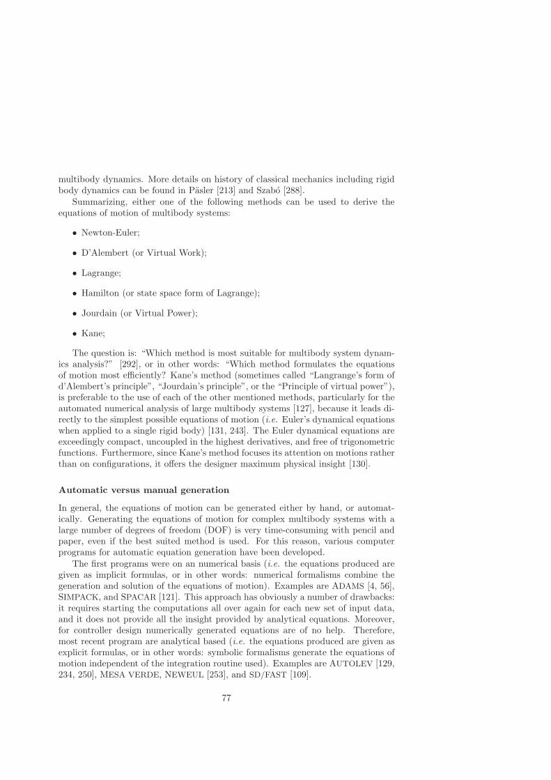
multibody dynamics. More details on history of classical mechanics including rigidbody dynamics can be found in Pasler [213] and Szabo [288].

Summarizing, either one of the following methods can be used to derive theequations of motion of multibody systems:

• Newton-Euler;

• D’Alembert (or Virtual Work);

• Lagrange;

• Hamilton (or state space form of Lagrange);

• Jourdain (or Virtual Power);

• Kane;

The question is: “Which method is most suitable for multibody system dynam-ics analysis?” [292], or in other words: “Which method formulates the equationsof motion most efficiently? Kane’s method (sometimes called “Langrange’s form ofd’Alembert’s principle”, “Jourdain’s principle”, or the “Principle of virtual power”),is preferable to the use of each of the other mentioned methods, particularly for theautomated numerical analysis of large multibody systems [127], because it leads di-rectly to the simplest possible equations of motion (i.e. Euler’s dynamical equationswhen applied to a single rigid body) [131, 243]. The Euler dynamical equations areexceedingly compact, uncoupled in the highest derivatives, and free of trigonometricfunctions. Furthermore, since Kane’s method focuses its attention on motions ratherthan on configurations, it offers the designer maximum physical insight [130].

Automatic versus manual generation

In general, the equations of motion can be generated either by hand, or automat-ically. Generating the equations of motion for complex multibody systems with alarge number of degrees of freedom (DOF) is very time-consuming with pencil andpaper, even if the best suited method is used. For this reason, various computerprograms for automatic equation generation have been developed.

The first programs were on an numerical basis (i.e. the equations produced aregiven as implicit formulas, or in other words: numerical formalisms combine thegeneration and solution of the equations of motion). Examples are ADAMS [4, 56],SIMPACK, and SPACAR [121]. This approach has obviously a number of drawbacks:it requires starting the computations all over again for each new set of input data,and it does not provide all the insight provided by analytical equations. Moreover,for controller design numerically generated equations are of no help. Therefore,most recent program are analytical based (i.e. the equations produced are given asexplicit formulas, or in other words: symbolic formalisms generate the equations ofmotion independent of the integration routine used). Examples are AUTOLEV [129,234, 250], MESA VERDE, NEWEUL [253], and SD/FAST [109].

77

The symbolic representation has the advantage that the equations of motion areto be generated only once, and the expressions have only to be evaluated during time-integration. The cost for the formulation of one symbolic set of equations is higherthan once running through a numerical formalism. However, symbolic equationsare an exact basis for the model under consideration, and combined with a packagefor numerical analysis, and simulation (e.g. MATLAB R©/SIMULINK R©) they result inten or even more times faster computations than a purely numerical approach wouldrequire [62, 140, 201, 243]. See Schiehlen [252] for a more detailed comparison ofimportant multibody system dynamics software.

We have decided to use SD/FAST R© for the generation of the equations of motionof flexible wind turbines within DAWIDUM’s mechanical module. The main reasonsare twofold. First, SD/FAST R© uses Kane’s method for the derivation of the equationsof motion. Second, it is able to generate SIMULINK R© MEX-files.

Main features of SD/FAST

SD/FAST R©, a product of Symbolic Dynamics, Inc., is a general-purpose multibodyprogram whose function it is to create special-purpose simulation code employing ex-plicit equations of motion for particular multibody configurations of interest. Com-puter symbol manipulation is used to simplify the general form of the equations ofmotion as appropriate to the system at hand (i.e. repeated terms are removed inorder to arrive at the computationally simplest equations).

Any mechanical system that can be described as a collection of hinge-connectedrigid bodies can be modeled in SD/FAST R©. The system topology can either be open-loop, tree, or closed-loop (see Fig. 3.17 for a graphical illustration). The systemscan be “free-flying” (e.g. a spacecraft) or “grounded” (e.g. a wind turbine). Thesystem complexity is limited to 300 rigid bodies and 1000 degrees of freedom.

Figure 3.17: Topological structures of multibody systems: (a) open-loop (or chain),(b) tree, and (c) closed-loop.

The connection between the bodies, or between a body and the ground is es-tablished by means of joints (e.g. translational joints, rotational joints, or sphericaljoints). These connections typically impose constraints on the relative motion be-

78

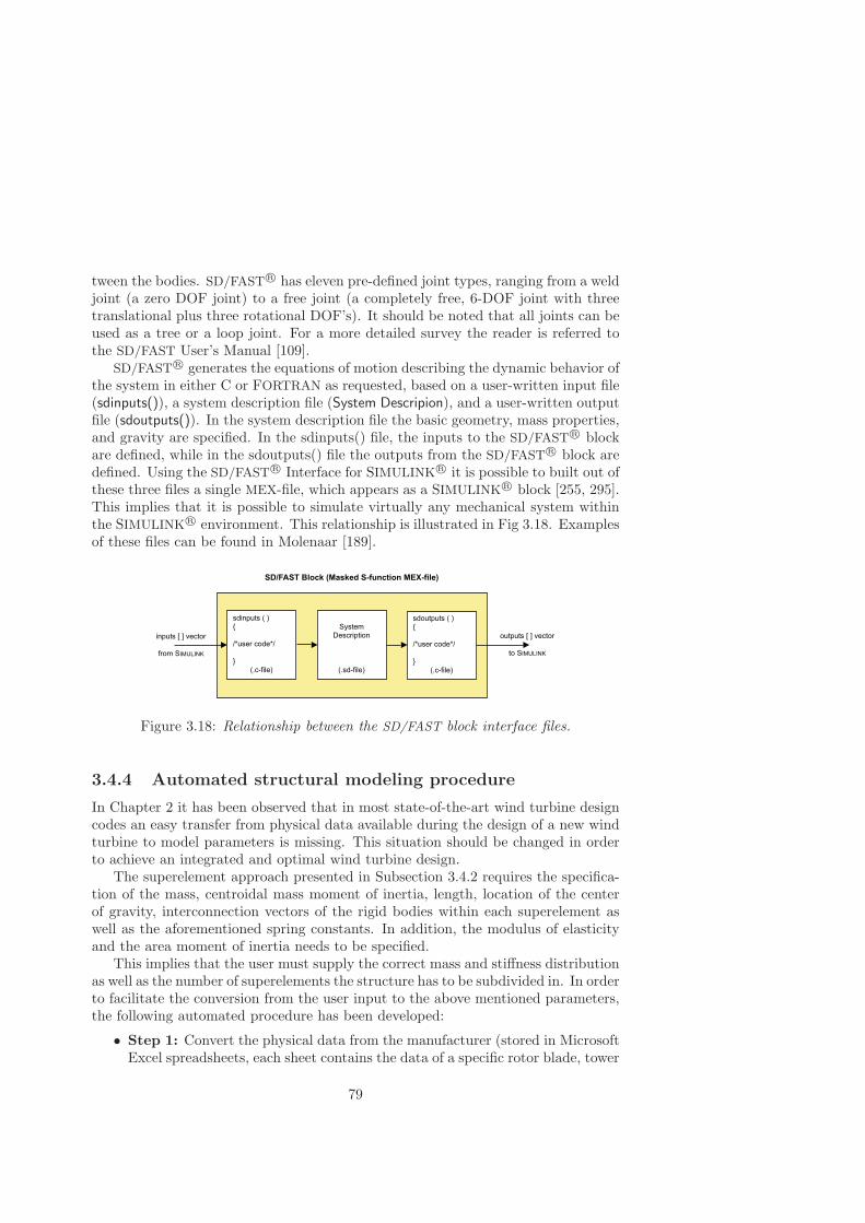
tween the bodies. SD/FAST R© has eleven pre-defined joint types, ranging from a weldjoint (a zero DOF joint) to a free joint (a completely free, 6-DOF joint with threetranslational plus three rotational DOF’s). It should be noted that all joints can beused as a tree or a loop joint. For a more detailed survey the reader is referred tothe SD/FAST User’s Manual [109].

SD/FAST R© generates the equations of motion describing the dynamic behavior ofthe system in either C or FORTRAN as requested, based on a user-written input file(sdinputs()), a system description file (System Descripion), and a user-written outputfile (sdoutputs()). In the system description file the basic geometry, mass properties,and gravity are specified. In the sdinputs() file, the inputs to the SD/FAST R© blockare defined, while in the sdoutputs() file the outputs from the SD/FAST R© block aredefined. Using the SD/FAST R© Interface for SIMULINK R© it is possible to built out ofthese three files a single MEX-file, which appears as a SIMULINK R© block [255, 295].This implies that it is possible to simulate virtually any mechanical system withinthe SIMULINK R© environment. This relationship is illustrated in Fig 3.18. Examplesof these files can be found in Molenaar [189].

Figure 3.18: Relationship between the SD/FAST block interface files.

3.4.4 Automated structural modeling procedure

In Chapter 2 it has been observed that in most state-of-the-art wind turbine designcodes an easy transfer from physical data available during the design of a new windturbine to model parameters is missing. This situation should be changed in orderto achieve an integrated and optimal wind turbine design.

The superelement approach presented in Subsection 3.4.2 requires the specifica-tion of the mass, centroidal mass moment of inertia, length, location of the centerof gravity, interconnection vectors of the rigid bodies within each superelement aswell as the aforementioned spring constants. In addition, the modulus of elasticityand the area moment of inertia needs to be specified.

This implies that the user must supply the correct mass and stiffness distributionas well as the number of superelements the structure has to be subdivided in. In orderto facilitate the conversion from the user input to the above mentioned parameters,the following automated procedure has been developed:

• Step 1: Convert the physical data from the manufacturer (stored in MicrosoftExcel spreadsheets, each sheet contains the data of a specific rotor blade, tower

79

or beam) into a multidimensional array stored in a MAT-file (i.e. RotorBlade-Data, TowerData, or BeamData respectively);

• Step 2: Select the model with the desired number of degrees of freedom out ofthe available mechanical module library (see Appendix I.2.3 for an overview);

• Step 3: Convert data in the MAT-file to SD/FAST R© input parameters by run-ning MATLAB R© M-file. The required SD/FAST parameters are stored in a ro-tor blade/tower/beam specific file with the specified number of superelementsappended to the basename “Blade”, “Tower” or “Beam” (e.g. Blade2.matcontains the SD/FAST data of a blade divided into 2 superelements);

• Step 4: Build SIMULINK R© MEX-file containing equations of motion by run-ning SD/FAST R©.

This systematic procedure has been implemented in DAWIDUM providing bothstructural designers and control engineers with a tool that enables them to rapidlyand easily build accurate dynamic models of flexible mechanical structures. In Ta-ble I.1 on page 273 an overview is given of the CPU time used to generate theequations of motion of several DAWIDUM models. It shows that this takes onlya few seconds even for the most complex structural model. In addition, becausethe user can determine the model complexity by specifying the number of superele-ments, the resulting models can be made suited for time-domain simulation, analysisof dynamic loads, or control design purposes. This implies that a bidirectional com-munication between the structural wind turbine design and the controller design hasbeen established.

It should be stressed that the presented mechanical module contains a modelof the structural dynamics of a complete flexible wind turbine. The spacers, hub,nacelle and both the stator and rotor of the generator are in general treated as rigid,while the support structure and rotor blades are to be modeled as flexible bodies.Flexible body dynamics are approximated using the aforementioned superelements.This integrated approach overcomes the shortcomings regarding the incomplete mod-eling of the “rotor - support structure”-interaction reported in Kuhn [144] and Wil-son [306].

3.4.5 Soil dynamics

Up to now, the effect of the flexibility of the foundation and its supporting soil hasnot been dealt with in this thesis. Soil is a non-linear material in which the stifnessprogressively decreases with increasing shear stress until, at a sufficient high stresslevel, plastic deformation takes place. Furthermore, when subjected to cyclic loading,soil exhibits damping which increases with increasing shear amplitude. Soil dampingcomprises two parts: internal and radiation. The internal damping (also calledmaterial, structural or hysteric damping) is mainly caused by viscous and frictionaleffects within the soil. The radiation damping is an elastic property associated withstress waves being propagated away from an area. Obviously, the soil propertiesvary from place to place, and many of the properties vary in time too.

80

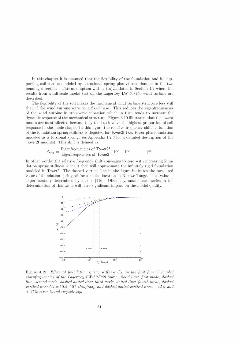
In this chapter it is assumed that the flexibility of the foundation and its sup-porting soil can be modeled by a torsional spring plus viscous damper in the twobending directions. This assumption will be (in)validated in Section 4.2 where theresults from a full-scale modal test on the Lagerwey LW-50/750 wind turbine aredescribed.

The flexibility of the soil makes the mechanical wind turbine structure less stiffthan if the wind turbine were on a fixed base. This reduces the eigenfrequenciesof the wind turbine in transverse vibration which in turn tends to increase thedynamic response of the mechanical structure. Figure 3.19 illustrates that the lowestmodes are most affected because they tend to involve the highest proportion of soilresponse in the mode shape. In this figure the relative frequency shift as functionof the foundation spring stiffness is depicted for Tower2f (i.e. tower plus foundationmodeled as a torsional spring, see Appendix I.2.3 for a detailed description of theTower2f module). This shift is defined as:

∆ωf =Eigenfrequencies of Tower2f

Eigenfrequencies of Tower2· 100 − 100 [%]

In other words: the relative frequency shift converges to zero with increasing foun-dation spring stiffness, since it then will approximate the infinitely rigid foundationmodeled in Tower2. The dashed vertical line in the figure indicates the measuredvalue of foundation spring stiffness at the location in Nieuwe-Tonge. This value isexperimentally determined by Jacobs [116]. Obviously, small inaccuracies in thedetermination of this value will have significant impact on the model quality.

109

1010

1011

1012

−100

−90

−80

−70

−60

−50

−40

−30

−20

−10

0

Cf [Nm/rad]

∆ω

f [%

]

− 25% + 25%

Figure 3.19: Effect of foundation spring stiffness Cf on the first four uncoupledeigenfrequencies of the Lagerwey LW-50/750 tower. Solid line: first mode, dashedline: second mode, dashed-dotted line: third mode, dotted line: fourth mode, dashedvertical line: Cf = 19.4 · 10 9 [Nm/rad], and dashed-dotted vertical lines: - 25% and+ 25% error bound respectively.

81

3.4.6 Example: three bladed wind turbine

For the purpose of illustration, Fig. 3.20 shows a superelement approximation ofa three bladed wind turbine. Observe that both the tower and rotor blades areapproximated by one superelement. Each superelement consists of three rigid bodiesconnected by two joints (marked ). Each joint (i.e. a universal joint since bothblade and tower torsion is not considered in this thesis) has two degrees of freedom.This implies that this system has 18-DOF (exclusive pitch and azimuth). Obviously,the total number of degrees of freedom required for proper modeling depends on boththe wind turbine and site under investigation.

Figure 3.20: Superelement approximation of a three bladed wind turbine, with :universal joints (2-DOF rotational joints). Both the tower and rotor blades areapproximated by one superelement consisting of 3 rigid bodies connected by idealtorsional springs. The flexibility of the foundation is approximated by a torsionalspring.

Please remember that the resulting model accuracy strongly depends on the qual-ity of the input data (i.e. garbage-in is by definition garbage-out). For example,in case of a wind turbine the uncertain (mechanical) parameters are particularlyfound in the area of foundation stiffness and damping. Obviously, when the corre-lation with the test data is not satisfactory, there is a need to modify the model bytuning/updating the model parameters. Since ad hoc procedures (trial and error)become impractical for more than three or four parameters, a systematic procedurehas to be developed. This subject is treated in Chapter 5.

82

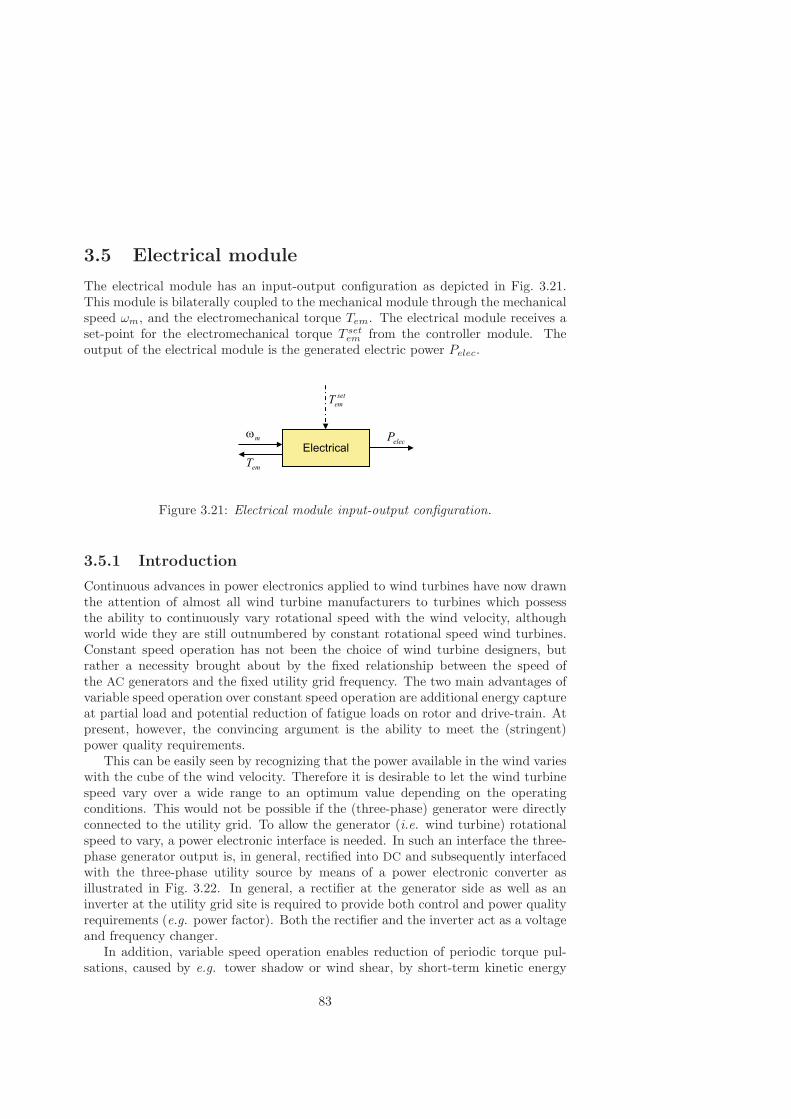
3.5 Electrical module

The electrical module has an input-output configuration as depicted in Fig. 3.21.This module is bilaterally coupled to the mechanical module through the mechanicalspeed ωm, and the electromechanical torque Tem. The electrical module receives aset-point for the electromechanical torque T set

em from the controller module. Theoutput of the electrical module is the generated electric power Pelec.

Electricalm

emT

elecP

set

emT

Figure 3.21: Electrical module input-output configuration.

3.5.1 Introduction

Continuous advances in power electronics applied to wind turbines have now drawnthe attention of almost all wind turbine manufacturers to turbines which possessthe ability to continuously vary rotational speed with the wind velocity, althoughworld wide they are still outnumbered by constant rotational speed wind turbines.Constant speed operation has not been the choice of wind turbine designers, butrather a necessity brought about by the fixed relationship between the speed ofthe AC generators and the fixed utility grid frequency. The two main advantages ofvariable speed operation over constant speed operation are additional energy captureat partial load and potential reduction of fatigue loads on rotor and drive-train. Atpresent, however, the convincing argument is the ability to meet the (stringent)power quality requirements.

This can be easily seen by recognizing that the power available in the wind varieswith the cube of the wind velocity. Therefore it is desirable to let the wind turbinespeed vary over a wide range to an optimum value depending on the operatingconditions. This would not be possible if the (three-phase) generator were directlyconnected to the utility grid. To allow the generator (i.e. wind turbine) rotationalspeed to vary, a power electronic interface is needed. In such an interface the three-phase generator output is, in general, rectified into DC and subsequently interfacedwith the three-phase utility source by means of a power electronic converter asillustrated in Fig. 3.22. In general, a rectifier at the generator side as well as aninverter at the utility grid site is required to provide both control and power qualityrequirements (e.g. power factor). Both the rectifier and the inverter act as a voltageand frequency changer.

In addition, variable speed operation enables reduction of periodic torque pul-sations, caused by e.g. tower shadow or wind shear, by short-term kinetic energy

83

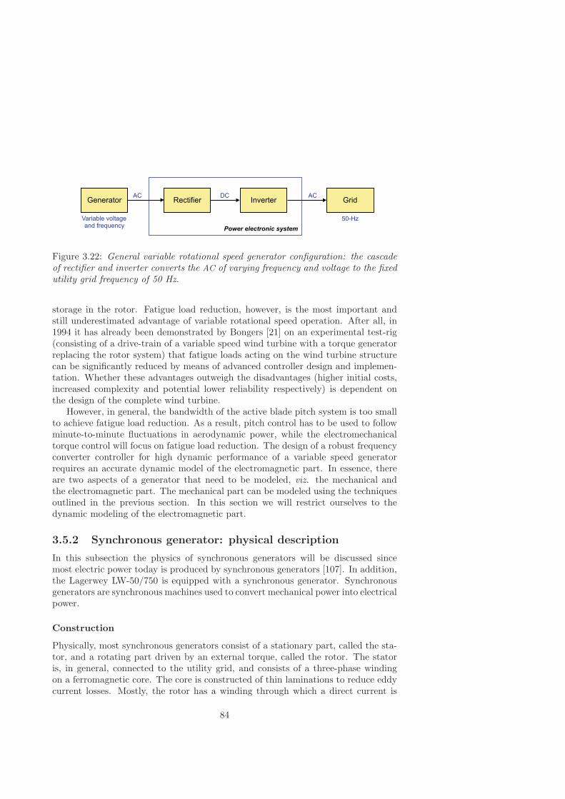
Figure 3.22: General variable rotational speed generator configuration: the cascadeof rectifier and inverter converts the AC of varying frequency and voltage to the fixedutility grid frequency of 50 Hz.

storage in the rotor. Fatigue load reduction, however, is the most important andstill underestimated advantage of variable rotational speed operation. After all, in1994 it has already been demonstrated by Bongers [21] on an experimental test-rig(consisting of a drive-train of a variable speed wind turbine with a torque generatorreplacing the rotor system) that fatigue loads acting on the wind turbine structurecan be significantly reduced by means of advanced controller design and implemen-tation. Whether these advantages outweigh the disadvantages (higher initial costs,increased complexity and potential lower reliability respectively) is dependent onthe design of the complete wind turbine.

However, in general, the bandwidth of the active blade pitch system is too smallto achieve fatigue load reduction. As a result, pitch control has to be used to followminute-to-minute fluctuations in aerodynamic power, while the electromechanicaltorque control will focus on fatigue load reduction. The design of a robust frequencyconverter controller for high dynamic performance of a variable speed generatorrequires an accurate dynamic model of the electromagnetic part. In essence, thereare two aspects of a generator that need to be modeled, viz. the mechanical andthe electromagnetic part. The mechanical part can be modeled using the techniquesoutlined in the previous section. In this section we will restrict ourselves to thedynamic modeling of the electromagnetic part.

3.5.2 Synchronous generator: physical description

In this subsection the physics of synchronous generators will be discussed sincemost electric power today is produced by synchronous generators [107]. In addition,the Lagerwey LW-50/750 is equipped with a synchronous generator. Synchronousgenerators are synchronous machines used to convert mechanical power into electricalpower.

Construction

Physically, most synchronous generators consist of a stationary part, called the sta-tor, and a rotating part driven by an external torque, called the rotor. The statoris, in general, connected to the utility grid, and consists of a three-phase windingon a ferromagnetic core. The core is constructed of thin laminations to reduce eddycurrent losses. Mostly, the rotor has a winding through which a direct current is

84

flowing: the field winding. The field winding produces a rotor magnetic field. Thisrotating magnetic field induces a three-phase set of AC voltages within the statorwindings of the generator. The magnetic field created by the stator windings reactswith the rotating field thereby producing an electromagnetic torque. This torqueis the mechanism through which the synchronous generator converts mechanical toelectrical energy.

Since the rotor is rotating, a special arrangement is required to get the DC powerto the field windings. There are two common approaches: either via an external DC

source by means of slip rings and brushes or via a special DC power source mounteddirectly on the synchronous generator shaft. Slip rings and brushes were used on allsmaller synchronous machines, while on larger generators and motors the DC poweris provided by the latter approach [44]. The DC power required for excitation takesapproximately one to a few percent of the rating of the synchronous generator [63].

The DC excitation of the field winding can also be provided by permanent mag-nets. Permanent magnet excitation brings the following benefits: i) higher torque oroutput power per volume, and ii) elimination of rotor copper losses due to the absenceof electrical excitation, implying a substantial increase in the efficiency [92, 286]. Themain disadvantages are: i) the field is uncontrollable [108], and ii) the assembly is atricky job.

Depending on the rotor construction, a synchronous machine may be either around-rotor (or cylindrical), or a salient-pole type. Figure 3.23 shows the cross-sections of both types. The salient-pole construction is mostly used in low-speedapplications where the diameter to length ratio can be made larger to accommodatethe higher pole number (20 up to 120 poles). This results in ring-generators. Anexample of this type is the synchronous generator used in waterwheel turbines. Theround-rotor construction is favoured in high-speed applications where the diameterto length ratio has to be kept small to keep the mechanical stresses from centrifugalforces within acceptable limits. Examples are synchronous generators driven bysteam or gas turbines.

Figure 3.23: Cross-section of a two-pole round, and on a four-pole salient-pole rotor.

85

Synchronous speed

Synchronous generators are by definition synchronous, meaning that the producedelectrical angular frequency with constant rotor field excitation is locked in or syn-chronized with the mechanical speed of the stator magnetic field, or equivalentlythe generator shaft speed. The produced frequency is completely determined by thegenerator shaft speed and the number of pole-pairs

f =p · n60

(3.69)

where f the produced frequency in hertz, p the number of pole-pairs, and n is thespeed of the generator shaft expressed in rotations per minute (r.p.m.). For example,to generate 50-Hz power in a four pole machine, the rotor must turn at 1500 r.p.m.This relationship is depicted in Table 3.2.

Table 3.2: Relationship between number of pole-pairs p, and rotational speed n of athree-phase synchronous generator linked to a grid with a fixed 50-Hz frequency.

Large wind turbines have relatively low rotor shaft speeds, typically from 50 to15 r.p.m. in the power range from 300 to 1500 kW, while wind turbine generatorstypically have 2, 3, or 4 pole-pairs (with base speeds of 1500, 1000 and 750 r.p.m.respectively at 50-Hz grid frequency, see Table 3.2). Consequently, if we want tolink such a wind turbine driven generator to the grid with a fixed 50-Hz frequency,a mechanical transmission with a speed ratio between 10 and 100 is required toincrease the angular velocity of the rotor shaft in order to come to an angular velocitywell-suited for the (high-speed) generator. Most wind turbines are equipped witha rotor-transmission-generator drive-train where the combination of generator basespeed and transmission ratio is selected such that the drive-train costs are minimized[106].

The interest in low-speed generators (which are directly connected to the shaftof the turbine and hence eliminating the transmission) has increased significantly inthe past decade [92]. These so-called direct-drive generators necessarily have a largediameter, because it follows from basic generator theory that the torque that can beproduced is directly related to the volume of the generator [298]. This constructionoffers a number of advantages in comparison to its counterpart with transmission.The most important advantages are a reduced noise level and a reduction of installa-tion costs [186]. In addition, when combined with efficient, variable frequency powersupply allowing the rotational speed to vary with the wind velocity, the aforemen-tioned advantages can be obtained. The main disadvantages are the relatively highgenerator mass and the present purchase price.

86

3.5.3 Synchronous generator: mathematical description

The aim of this section is to set up a theoretical model of a synchronous generatorsuited for both time-domain simulation, and model based control design.

From a modeling point of view all synchronous generators have similar repre-sentations. They differ only with respect to some model parameters. Because theround-rotor synchronous generator is a special case of the salient-pole rotor syn-chronous generator, we will treat only the latter for an arbitrary number of pole-pairsp in this section.

Fig. 3.24 depicts a salient-rotor synchronous generator with only one pole-pair(p = 1 for illustration purposes). The machine has the usual three stator windings,each 120 (electrical) degrees apart. The stator windings are star connected. Therotor has one accessible circuit, the field or excitation winding, and two sets ofinaccessible circuits, called damper windings. Damper windings are real or fictitiouswindings that can be used to represent, for example, the damping effects of eddycurrents in the machine. In Fig. 3.24, one damper winding is located along the direct-axis, and one along the quadrature-axis (represented by ψ1d and ψ1q in Fig. 3.24).When the DC excitation of the field winding is provided by permanent magnets, thefield windings can be replaced by fictitious ones carrying constant field currents.

Figure 3.24: Schematic representation of an elementary three-phase, two-pole syn-chronous generator.

3.5.4 Dynamic generator model

The operation of a (synchronous) generator is based on the Maxwell’s second equa-tions or equivalently, Faraday’s law of electromagnetic induction. This law statesthat when the field is excited and rotated, voltages will be induced in the threestator phases.

87

The fields produced by the stator winding currents are assumed to be sinusoidallydistributed around the airgap. This assumption ignores the space harmonics andas a result, the induced stator voltages (or electromagnetic force EMF) will varysinusoidally with time. In steady-state, the three sine waves will be displaced 120

electrical degrees in time as a result of the phases being displaced 120 in space.Using generator sign convention, the stator currents are defined positive flowing outof the machines terminals and the expressions for the induced stator voltages become

ua = −Ra · ia − dψa

dt

ub = −Rb · ib − dψb

dt(3.70)

uc = −Rc · ic − dψc

dt

with Ra, Rb, and Rc the resistance of stator a-phase, b-phase and c-phase, ia, iband ic the stator currents, and ψa, ψb and ψc the stator flux linkages respectively.The stator resistances are constant when skin effect and effects of temperature areneglected [219].

The equation for the field winding voltage is

−uf = −Rf · if − dψf

dt(3.71)

with Rf , if and ψf the field winding resistance, current, and flux linkage respectively.The equations for the short-circuited (i.e. u1d = 0) direct-axis damper winding andshort-circuited (i.e. u1q = 0) quadrature-axis damper winding are

u1d = −R1d · i1d − dψ1d

dt= 0

u1q = −R1q · i1q − dψ1q

dt= 0

(3.72)

with R1d (R1q), i1d (i1q) and ψ1d (ψ1q) the d (q)-axis damper resistance, current, andflux linkages respectively. Here it is assumed that the damping can be adequatelyrepresented by one damper winding on the direct-axis and one on the quadrature-axis.

The voltage equations of the rotor and stator windings can be arranged in thefollowing matrix form[

us

ur

]= −

[Rs 00 Rr

]·[

isir

]− d

dt

[ψs

ψr

](3.73)

where

us =[ua ub uc

]Tur =

[ −uf 0 0]T

Rs = diag[Ra Rb Rc

]88

Rr = diag[Rf R1d R1q

]is =

[ia ib ic

]Tir =

[if i1d i1q

]Tψs =

[ψa ψb ψc

]Tψr =

[ψf ψ1d ψ1q

]TIt is assumed that the flux linkages ψs, and ψr in Eq. (3.73) are linearly related

to the six currents ia, ib, ic, if , i1d, and i1q by a 6 × 6 inductance matrix

ψa

ψb

ψc

ψf

ψ1d

ψ1q

=

Laa Lab Lac Laf La1d La1q

Lba Lbb Lbc Lbf Lb1d Lb1q

Lca Lcb Lcc Lcf Lc1d Lc1q

Lfa Lfb Lfc Lff Lf1d Lf1q

L1da L1db L1dc L1df L1d1d L1d1q

L1qa L1qb L1qc L1qf L1q1d L1q1q

·

iaibicifi1d

i1q

(3.74)

where self-inductances are denoted by two like subscripts, and mutual inductancesare denoted by two unlike subscripts. In matrix form[

ψs

ψr

]=

[Lss Msr

Mrs Lrr

]·[

isir

](3.75)

where Lss represents the stator self-inductance matrix, and Lrr represents the rotorself-inductance matrix. The stator-rotor and rotor-stator mutual inductances arerepresented by Msr and Msr respectively.

The synchronous generator is thus represented as a group of magnetically coupledcircuits. The circuits are shown schematically in Fig. 3.25. Each of the windingshas thus its own resistance, self-inductance and mutual inductances with respectto every other winding. Notice that most inductances in Eq. (3.75) depend on theangular position of the rotor [222].

Inductances of salient-pole generator

The self-inductance of any stator winding varies periodically from a maximum (whenthe direct-axis coincides with the phase axis) to a minimum (when the quadrature-axis is in line with the phase axis). The self-inductance Laa for example, will reacha maximum for θe = 0, a minimum for θe = 90 and maximum again for θe = 180

and so on. That is, Laa has a period of θe = 180 electrical degrees and can beexactly represented by a series of cosines of even harmonics of angle [246]. Becauseof the rotor symmetry, the diagonal elements of the submatrix Lss are representedas

Laa = Ls + Lm cos 2 (θe)Lbb = Ls + Lm cos 2

(θe − 2

3π)

(3.76)

Lcc = Ls + Lm cos 2(θe + 2

3π)

89

Figure 3.25: Schematic representation of mutually coupled circuits.

where both Ls and Lm are constants (Ls > Lm), and θe is the angle betweenthe direct-axis and the magnetic axis of phase a in electrical degrees as shown inFig. 3.24. Since the angle included in one pole pair p is 360 electrical degrees, theangle θe in electrical units is related to the mechanical angle θm through the numberof pole-pairs p as follows

θe = p θm

The air gap of a salient-pole synchronous generator varies along the inner circum-ference of the stator. Consequently the mutual inductances between any two statorphases are also periodic functions of the electrical angle θe, and hence vary with time.It can be concluded from symmetry considerations that the mutual inductance be-tween phase a and b should have a negative maximum when the pole axis is linedup 30 behind phase a, or 30 ahead of phase b, and a negative minimum when it ismidway between the two phases. Thus, for a machine with sinusoidally-distributedwindings, the variations of the stator mutual inductances, i.e. the off-diagonal ele-ments of submatrix Lss can be represented as follows

Lab = Lba = −Ms − Lm cos 2(θe + 1

6π)

Lbc = Lcb = −Ms − Lm cos 2(θe − 1

2π)

(3.77)

Lca = Lac = −Ms − Lm cos 2(θe + 5

6π)

where |Ms| > Lm [246]. Notice that the signs of the mutual inductance terms dependupon assumed current directions and circuit orientation.

The elements of the submatrix Lrr consist of rotor self-inductances and mutualinductance between any two circuits both in direct-axis (or in quadrature-axis). Allthe rotor self-inductances, i.e. the diagonal elements of submatrix Lrr, are constantsince the effects of stator slots and saturation are neglected. They are represented

90

with single subscript notation

Lff = Lf

L1d1d = L1d (3.78)L1q1q = L1q

The mutual inductance between any two circuits both in direct-axis (or both inquadrature-axis) is constant. The mutual inductance between any rotor direct-axiscircuit and quadrature-axis circuit does not exist, thus

Lf1d = L1df = Mr

Lf1q = L1qf = 0 (3.79)L1d1q = L1q1d = 0

This are the off-diagonal elements of submatrix Lrr.Finally, consider the mutual inductances between stator and rotor circuits. Ob-

viously, these are periodic functions of the electrical angle θe. Because only thespace-fundamental component of the produced flux links the sinusoidally distributedstator, all stator-rotor mutual inductances vary sinusoidally, reaching a maximumwhen the two windings in question align. Thus, their variations can be written asfollows

Laf = Lfa = Mf cos θe

Lbf = Lfb = Mf cos(θe − 2

3π)

Lcf = Lfc = Mf cos(θe + 2

3π)

La1d = L1da = M1d cos θe

Lb1d = L1db = M1d cos(θe − 2

3π)

(3.80)

Lc1d = L1dc = M1d cos(θe + 2

3π)

La1q = L1qa = M1q sin θe

Lb1q = L1qb = M1q sin(θe − 2

3π)

Lc1q = L1qc = M1q sin(θe + 2

3π)

It follows from above equations that the rotor-stator mutual inductance matrix isequal to the transpose of the stator-rotor mutual inductance matrix. Thus, Msr =MT

rs in Eq. (3.75).The dynamic behavior of a synchronous, salient-pole generator is thus described

by Eq. (3.73) and the time-varying coefficients are given by Eqs. (3.76)-(3.80). Anal-ysis of the dynamic behavior can thus be accomplished by the solution of a set ofsimultaneous coupled-circuit differential equations. The solution of these equationsis complicated due to the fact that the inductances between the stator-phase wind-ings and the rotor circuits are a function of the rotor angle θe (and hence change withtime). This complication can be avoided by using Park’s transformation [211, 212].

91

Park’s transformation

The key idea of Park’s transformation is to express the stator flux linkages in therotating d, q reference system instead of the normal stator fixed reference system.The stator windings are replaced with two fictitious windings which are fixed withrespect to the rotor. One winding is chosen to coincide with the direct-axis, and theother with the quadrature-axis.

Since the axes of the rotor windings are already along the direct and quadrature-axes, the transformation needs only to be applied to the stator quantities. In orderto ensure that the rotor quantities remain unaffected, Park’s transformation matrixT0dq is expanded with a 3 × 3 identity matrix I3 as follows

C =[

T0dq 00 I3

](3.81)

with

T0dq =√

23

1√

21√2

1√2

cos(p θm) cos(p θm − 23π) cos(p θm + 2

3π)sin(p θm) sin(p θm − 2

3π) sin(p θm + 23π)

(3.82)

Notice the resemblance between Park’s transformation matrix and the presence ofthe sine and cosine terms in Eq. (3.80).

By definition, the transformed voltages, currents and flux linkages of the statorare given by

u0dq = T0dq · us

i0dq = T0dq · isψ0dq = T0dq · ψs

where

u0dq =[u0 ud uq

]Ti0dq =

[i0 id iq

]Tψ0dq =

[ψ0 ψd ψq

]TPremultiplying Eq. (3.75) by the transformation matrix C, the flux linkage equationsbecome [

T0dq 00 I3

] [ψs

ψr

]︸ ︷︷ ︸

ψ0dq

ψr

=

=[

T0dq 00 I3

] [Lss Msr

Mrs Lrr

] [T−1

0dq 00 I3

]·[

T0dq 00 I3

] [isir

]︸ ︷︷ ︸

i0dq

ir

92

or equivalently[ψ0dq

ψr

]=[

T0dq 00 I3

] [Lss Msr

Mrs Lrr

] [T−1

0dq 00 I3

]·[

i0dq

ir

](3.83)

Substituting the expressions for T0dq, T−10dq and the inductances given by Eqs. (3.76)-

(3.80), it can be shown that the above equation reduces to the following expressionin which all the inductances are independent of the rotor angle θe

ψ0

ψd

ψq

ψf

ψ1d

ψ1q

=

Lo 0 0 0 0 00 Ld 0 kMf kM1d 00 0 Lq 0 0 kM1q

0 kMf 0 Lf Mr 00 kM1d 0 Mr L1d 00 0 kM1q 0 0 L1q

︸ ︷︷ ︸L

·

i0idiqifi1d

i1q

(3.84)

where

L0 = Ls − 2Ms (3.85)Ld = Ls +Ms + 3

2 Lm (3.86)Lq = Ls +Ms − 3

2 Lm (3.87)

the self-inductances of the equivalent circuits, and k =√

32 . Note that the inductance

matrix L is sparse, symmetric and constant. The reader should compare it with theinductance matrix in Eq. (3.74) which depends on θe = p θm in a complicated way.

Obviously, the coupling between the rotor and stator of the direct-axis involvesthe factor k, and similarly for the quadrature-axis. For example, the contributionto the direct-axis stator flux linkage ψd due to the field current if is kMf if andso on. The self-inductances L0, Ld, and Lq are known as the zero-sequence induc-tance, the direct-axis synchronous inductance, and the quadrature-axis synchronousinductance, respectively [246].

Applying the transformation C to Eq. (3.73) gives the following voltage equationsin the dq reference frame[

u0dq

ur

]= −

[T0dq 00 I3

] [Rs 00 Rr

] [T−1

0dq 00 I3

] [i0dq

ir

]

−[

T0dq 00 I3

]d

dt

([T−1

0dq 00 I3

] [ψ0dq

ψr

])(3.88)

where

u0dq =[u0 ud uq

]TRs = diag

[Ra Rb Rc

]i0dq =

[i0 id iq

]T93

ψ0dq =[ψ0 ψd ψq

]Tur =

[ −uf 0 0]T

Rr = diag[Rf R1d R1q

]ir =

[if i1d i1q

]Tψr =

[ψf ψ1d ψ1q

]TEvaluating the first term while assuming that Ra = Rb = Rc = Rs, and obtainingthe derivative of the second term in Eq. (3.88), yields[

u0dq

ur

]= −

[Rs 00 Rr

] [i0dq

ir

]

−[

T0dq · ddt

(T−1

0dq

)0

0 0

] [ψ0dq

ψr

]− d

dt

[ψ0dq

ψr

](3.89)

The expression for T0dq · ddt

(T−1

0dq

)can be written as

T0dqd

dt

(T−1

0dq

)= T0dq

dθm

dt

d

dθm

(T−1

0dq

)= ωm T0dq

d

dθm

(T−1

0dq

)(3.90)

with

d

dθmT−1

0dq = p√

23

0 − sin(p θm) cos(p θm)

0 − sin(p θm − 23π) cos(p θm − 2

3π)0 − sin(p θm + 2

3π) cos(p θm + 23π)

(3.91)

Substituting this result, and T0dq from Eq. (3.82) into Eq. (3.90) gives

ωm T0dqd

dθm

(T−1

0dq

)=

1√

21√2

1√2

cos(pωm) cos(pωm − 23π) cos(pωm + 2

3π)sin(pωm) sin(pωm − 2

3π) sin(pωm + 23π)

·

pωm23

0 − sin(pωm) cos(pωm)

0 − sin(pωm − 23π) cos(pωm − 2

3π)0 − sin(pωm + 2

3π) cos(pωm + 23π)

= pωm

0 0 0

0 0 10 −1 0

(3.92)

Back-substituting the above results in Eq. (3.88) gives the following voltagesequations of an ideal synchronous generator (i.e. linear magnetic circuit and sta-tor windings are sinusoidally distributed along the stator circumference) in the dqreference frame in matrix form[

u0dq

ur

]= −

[Rs 00 Rr

] [i0dq

ir

]

94

−

pωm

0 0 0

0 0 10 −1 0

0

0 0

[ψ0dq

ψr

]− d

dt

[ψ0dq

ψr

](3.93)

Notice that Eq. (3.93) contains both currents and flux linkages as variables. Sincethese two sets of variables are mutually dependent, it is also possible to select theflux linkages as state variables [3]. Another observation is that the zero-sequenceequation

u0 = −R0 · i0 − L0d

dti0

is not coupled to the other equations. Therefore, it can be treated separately. Inaddition, in the vast majority of cases the generator is either connected in star suchthat the neutral current i0 does not flow (i.e. neutral point is isolated) or is Deltaconnected (were no neutral exists), implying that the zero-sequence equation canbe omitted [107, 202]. In the sequel the zero-sequence equation is omitted since thepower in the Lagerwey LW-50/750 wind turbine is generated in two star connectedthree-phase systems with the neutral points isolated(see Appendix A.4).

Substituting Eq. (3.84) in Eq. (3.93), omitting the zero-sequence equation yields

ud

−uf

0uq

0

=

−

Rs 0 0 pωm Lq pωm kM1q

0 Rf 0 0 00 0 R1d 0 0

−pωmLd −pωm kMf −pωm kM1d Rs 00 0 0 0 R1q

idifi1d

iqi1q

−

Ld kMf kM1d 0 0kMf Lf Mr 0 0kM1d Mr L1d 0 0

0 0 0 Lq kM1q

0 0 0 kM1q L1q

d

dt

idifi1d

iqi1q

(3.94)

This complete set of equations consisting of flux-linkage relations and voltage equa-tions are known as Park’s equations. The equations have been rearranged in or-der to show the coupling between the direct-axis and the quadrature-axis moreclearly. From the above equation follows that if the generator speed pωm is con-stant, the resulting Park’s equations are linear with constant coefficients. Noticethat at standstill (i.e. ωm = 0), there is no interaction between the direct-axis andthe quadrature-axis.

It should be noted that, in his original paper, R.H. Park used the non-powerinvariant transformation to transform the stator quantities onto the dq reference

95

frame that is fixed to the rotor. In the above derivation we have used the power-invariant version in order to ensure that in both reference frames the same powerexpressions are obtained. In addition, he used motor sign convention for the statorcircuits.

Park’s equations (reformulated)

Park’s equations are in the presented form not suited for time-domain simulationsince they contain a number of variables that can not be measured in practice (i.e.i1d, i1q, ψ1d, and ψ1q). It will be shown below that it is possible to eliminate thesevariables via substitution and rearranging of the aforementioned equations. Whenthe generator speed is constant and equal to pωm, the differential equations arelinear with constant coefficients. This implies that Eq. (3.84) may be transformedto the Laplace domain as follows

Ψd = LdId + kMfIf + kM1dI1d

Ψq = LqIq + kM1qI1q

Ψf = kMfId + LfIf +MrI1d (3.95)Ψ1d = kM1dId +MrIf + L1dI1d

Ψ1q = kM1qIq + L1qI1q

where k =√

32 . Notice that capitals indicate Laplace-transformed quantities, and

that zero initial conditions are assumed.Applying the Laplace transform to Eq. (3.93) with the assumption of zero initial

conditions gives

Ud = −RsId − sΨd − pωmΨq

Uq = −RsIq − sΨq + pωmΨd

Uf = RfIf + sΨf (3.96)0 = −R1dI1d − sΨ1d

0 = −R1qI1q − sΨ1q

where it again is assumed that Ra = Rb = Rc = Rs. The zero-sequence equationhas been omitted.

The transformed variables will now be eliminated via substitution and rearrang-ing, first for the direct-axis, and secondly for the quadrature-axis:

• Direct-axis. The equation for the field winding voltage, and the equation forthe voltage across the direct-axis damper are given by

Uf = RfIf + sΨf 0 = −R1dI1d − sΨ1d

The flux linkage equations on the direct-axis are given by

Ψd = LdId + kMfIf + kM1dI1d

Ψf = kMfId + LfIf +MrI1d

Ψ1d = kM1dId +MrIf + L1dI1d

96

Rewriting the flux linkage expressions and substituting the results in the volt-age equations allows elimination of If , I1d, Ψf and Ψ1d, resulting in the fol-lowing equation for the direct-axis stator flux

Ψd = LdId1 + (σfτf + σ1dτ1d)s

1 + (τf + τ1d)s+ (σrτfτ1d)s 2

+ LdId(τfτ1d · (σr − µ1d(1 − σf ) − µf (1 − σ1d)))s 2

1 + (τf + τ1d)s+ (σrτfτ1d)s 2(3.97)

+ kMfUf

Rf

1 + (τ1dµ1d)s1 + (τf + τ1d)s+ (σrτfτ1d)s 2

whereτf =

Lf

Rfτ1d =

L1d

R1d

the rotor time constants for the direct-axis,

σr = 1 − M 2r

LfL1dσf = 1 − k 2M 2

f

LdLfσ1d = 1 − k 2M 2

1d

LdL1d

the leakage factors, and

µf = 1 − MfMr

LfM1dµ1d = 1 − M1dMr

L1dMf

Furthermore, it is clear from Eq. (3.97) that the direct-axis stator flux is fre-quency dependent, and that its DC-gain is equal to Ld (for uf = 0), or equalto kMf/Rf (for id = 0). In the sequel, these DC-gains are referred to as LDC

d ,and −GDC

fd .

However, Eq. (3.97) is valid only for the situation that the (fictitious) damperwinding can be adequately represented by one winding located on the direct-axis. Recall that the number of damper windings depends on both the physicalconstruction of the rotor and the accuracy required by the model. More gen-eral, the direct-axis stator flux equation is described by

Ψd(s) = Ld(s)Id(s) −Gfd(s)Uf (s) (3.98)

where Ld(s) and Gfd(s) transfer functions. The order of the numerator anddenominator polynomials of Ld(s) are equal to the number of damper wind-ings located on the d-axis plus the field winding, while Gfd(s) has the samedenominator as Ld(s), but a different numerator. The order of the numeratorof Gfd(s) is one less than the denominator. Both transfer functions dependon the design of the synchronous generator and Ld(s) is usually referred to as“operational inductance”.

In addition, it is shown in Appendix D that

Ψd(s) = Ldo(s)Id(s) + Ldfo(s)If (s) (3.99)

97

and thatΨf (s) = Lfdo(s)Id(s) + Lfo(s)If (s) (3.100)

where Ldo(s), Lfdo(s) = Ldfo(s), and Lfo(s) are proper transfer functions,which depend on the design of the synchronous generator.

• Quadrature-axis. The equation for the voltage across the quadrature-axisdamper is given by

0 = −R1qI1q − sΨ1q

The flux linkage equations on the quadrature-axis are given by

Ψq = LqIq + kM1qI1q

Ψ1q = kM1qIq + L1qI1q

Rearranging the latter two expressions and substituting the results in the volt-age equation allows elimination of I1q and Ψ1q, resulting in the following equa-tion for the quadrature-axis stator flux

Ψq = LqIq1 + τ1qσ1q · s

1 + τ1q · s (3.101)

where

τ1q =L1q

R1q

the rotor time constant for the quadrature-axis, and

σ1q = 1 − k 2M 21q

LqL1q

the leakage factor. Furthermore, it is clear from Eq. (3.101) that the quadra-ture-axis stator flux is frequency dependent, and that its DC-gain is equal toLq. In the sequel, the DC-gain is referred to as LDC

q .

However, Eq. (3.101) is valid only for the situation that the (fictitious) damperwinding can be adequately represented by one winding located on the quadra-ture-axis. More general, the quadrature-axis stator flux equation is describedby

Ψq(s) = Lq(s)Iq(s) (3.102)

where Lq(s) is a proper transfer function, which function depends on the designof the synchronous generator. The order of the numerator and denominatorpolynomials of Lq(s) are equal to the number of damper windings located onthe q-axis.

The voltage equations in the dq reference frame of the electromagnetic part of asynchronous generator have been given in matrix form in Eq. (3.93). Removing the

98

zero-sequence equation gives the following set of equations

ud = −Rsid − pωmψq − d

dtψd

uq = −Rsiq + pωmψd − d

dtψq (3.103)

−uf = −Rf if − d

dtψf

with ud the direct-axis voltage, Rs the stator-winding resistance, id the direct-axiscurrent, pωm the generator speed, ψq the quadrature-axis winding flux, t time, ψd

the direct-axis winding flux, uq the quadrature-axis voltage, iq the quadrature-axiscurrent, uf the field-winding voltage, Rf the field-winding resistance, if the field-winding current, and ψf the field-winding flux.

A few observations can be made, the most important one being that equations(3.103) are coupled via the fluxes. In addition, they depend on the generator speedpωm, thereby introducing non-linearities. For time-domain simulation purposes, itis convenient to rewrite the this set of equations in the following form

ψd = −∫

(ud +Rsid + pωmψq) dt

ψq = −∫

(uq +Rsiq − pωmψd) dt (3.104)

ψf =∫

(uf −Rf if ) dt

with the fluxes as state variables.The fluxes, in turn, have been given by

Ψd(s)(3.99)= Ldo(s)Id(s) + Ldfo(s)If (s)

Ψq(s)(3.102)

= Lq(s)Iq(s) (3.105)

Ψf (s)(3.100)

= Lfdo(s)Id(s) + Lfo(s)If (s)

with s the Laplace operator and Ldo(s), Lfdo(s) = Ldfo(s), Lq(s), Lfo(s) propertransfer functions which can, for a finite number of damper windings, be expressedas a ratio of polynomials in s [147]. The direct-axis flux equations can be convenientlyexpressed in matrix form[

Ψd(s)Ψf (s)

]=[Ldo(s) Lfdo(s)Lfdo(s) Lfo(s)

]·[Id(s)If (s)

](3.106)

It can be easily shown that the inverse transformation is given by

[Id(s)If (s)

]=

[Lfo(s) −Lfdo(s)

−Lfdo(s) Ldo(s)

]Ldo(s) · Lfo(s) − L2

fdo(s)·[

Ψd(s)Ψf (s)

](3.107)

99

It is shown in Appendix D that the denominators of Ldo(s), Ldfo(s) = Lfdo(s),and Lfo(s) are all the same. Consequently, the denominators in the above matrixequation are identical.

Finally, the inverse of the quadrature-axis flux equation is given by

Iq(s) = Lq(s)−1Ψq(s) (3.108)

The dynamic behavior of an ideal synchronous generator is thus fully described bythe sets of equations (3.104), (3.107) and (3.108) expressed in the dq reference frame.These equations are implemented in DAWIDUM’s Elec2 module (see Appendix I.2.4).The resulting block diagram is depicted in Fig. 3.26.

Figure 3.26: Block diagram of an ideal synchronous machine.

Obviously, for simulation as well as control design purposes, accurate informa-tion about the transfer functions Ldo(s), Lfdo(s), Lq(s) and Lfo(s), as well as theresistances Rs and Rf , is required. In Section 4.3 a new procedure is developedfor identifying the transfer functions Yd(s) and Yq(s) (see Fig. 3.26) of Park’s dq-axis model of a synchronous generator from time-domain standstill test data. Tocomplete the analysis, relations for power and torque are needed.

100

Electromagnetic torque

The instantaneous power output of a three-phase synchronous generator is simplythe sum of the stator ui products

Pg = ua · ia + ub · ib + uc · ic (3.109)

It can be shown that by applying Park’s power-invariant transformation to Eq. (3.109),the following power output equation expressed in odq coordinates can be obtained

Pg = u0 · i0 + ud · id + uq · iq (3.110)

Assuming that the generator is star connected with the star point not used, thisequation reduces to

Pg = ud · id + uq · iq (i0 = 0) (3.111)

Substitution of ud and uq from Eq. (3.93) in Eq. (3.111) gives

Pg =(−Rs · id − pωmψq − dψd

dt

)· id +

(−Rs · iq + pωmψd − dψq

dt

)· iq

= −Rs

(i 2d + i 2q

)︸ ︷︷ ︸P s

cu

−(dψd

dtid +

dψq

dtiq

)+ pωm (ψd · iq − ψq · id)︸ ︷︷ ︸

Pem

(3.112)

The first term in Eq. (3.112) describes the power dissipated in the stator windings(the so-called stator copper losses). The second term corresponds to the time rateof change of the magnetic energy stored in the inductances of the generator, andthe third term reflects the power transferred across the airgap [211]. This power isequal to the electromechanical power developed, hence

Pem = pωm (ψd · iq − ψq · id) (3.113)

Dividing the electromechanical power by the mechanical speed of the generator shaft(ωm), the following expression is obtained for the instantaneous electromechanicaltorque developed by a synchronous generator with p pole-pairs

Tem = p (ψd · iq − ψq · id) (3.114)

The value of Tem from the above expression is negative for motoring, and positivefor generator operation.

Furthermore, it is assumed that the generated electrical power is equal to thegenerator power output minus the converter losses, the electric excitation losses (theso-called rotor copper losses) and the cable losses

Pelec = Pg − Pconv − P rcu − Pcable (3.115)

The converter losses include the switching losses in the power electronic interfaceand are, here, divided into no-load losses (which are constant) and losses which areproportional to the stator current squared

Pconv = C1 + (1 − ηconv − C1) · P relec ·

(isirs

)2

(3.116)

101

where P relec the rated electric power. The rotor copper losses are due to the excitation

current flowing through the resistance of the field winding and are given by

P rcu = i2fRf (3.117)

with if and Rf the field winding current and resistance respectively. The power lossin the cables is given by

Pcable = (1 − η rcable) · P elec

r ·(isirs

)2

(3.118)

with η rcable the cable efficiency at rated electric power and is the stator current.

As noted in Section 3.5, in the development of the dynamic model of a syn-chronous generator we have ignored the losses in the magnetic material. Thereare two main sources of losses: hysteresis and eddy current losses. The hysteresislosses are due to the fact that all magnetic cores exhibit some degree of hysteresisin their B-H characteristic. Consequently, a time-varying flux in the core will dis-sipate power. Eddy current losses are due to the existence of circulating currentswithin the body of a ferromagnetic material under conditions of a time-varying flux.These currents cause an undesirable heating effect. The magnitude of these lossescan be reduced by constructing the magnetic circuit from thin laminations of theferromagnetic material rather than the solid. The details of the physical mechanismsthat cause these losses are beyond the scope of this thesis, but can be found in theliterature.

Taken together the hysteresis losses and eddy current losses are often describedas the core, or iron losses. The iron losses are approximately proportional to thesquare of the voltage. However, in Polinder [219] it has been concluded that nosimple and exact analytical expression for the iron losses can be derived. Thereto itis preferred to determine the core losses experimentally. To account for both frictionand iron losses it is assumed that

Pem = Paero − Pfric − P sFe (3.119)

where Paero the aerodynamic power, Pfric the total amount of friction in the drivetrain and P s

Fe the stator iron losses. Summarizing, the power balance from aerody-namic power to generated electrical power is given by:

Pelec(3.115)

= Pg − Pconv − P rcu − Pcable

(3.112)= (Pem − P s

cu) − Pconv − P rcu − Pcable (steady-state)

= (Paero − Pfric − P sFe) − P s

cu − Pconv − P rcu − Pcable (3.120)

This relationship is graphically depicted in Fig. 3.27.This concludes the derivation of the equations describing a non-linear dynamic

model of a salient-pole synchronous generator if saturation of the magnetic circuit isnot considered. To account for saturation, it is necessary to replace the linear flux-current relationship, Eq. (3.74), by a non-linear one and subsequently repeating the

102

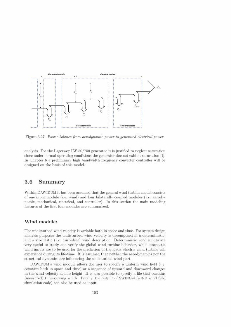
Figure 3.27: Power balance from aerodynamic power to generated electrical power.

analysis. For the Lagerwey LW-50/750 generator it is justified to neglect saturationsince under normal operating conditions the generator doe not exhibit saturation [1].In Chapter 6 a preliminary high bandwidth frequency converter controller will bedesigned on the basis of this model.

3.6 Summary

Within DAWIDUM it has been assumed that the general wind turbine model consistsof one input module (i.e. wind) and four bilaterally coupled modules (i.e. aerody-namic, mechanical, electrical, and controller). In this section the main modelingfeatures of the first four modules are summarized.

Wind module:

The undisturbed wind velocity is variable both in space and time. For system designanalysis purposes the undisturbed wind velocity is decomposed in a deterministic,and a stochastic (i.e. turbulent) wind description. Deterministic wind inputs arevery useful to study and verify the global wind turbine behavior, while stochasticwind inputs are to be used for the prediction of the loads which a wind turbine willexperience during its life-time. It is assumed that neither the aerodynamics nor thestructural dynamics are influencing the undisturbed wind part.

DAWIDUM’s wind module allows the user to specify a uniform wind field (i.e.constant both in space and time) or a sequence of upward and downward changesin the wind velocity at hub height. It is also possible to specify a file that contains(measured) time-varying winds. Finally, the output of SWING-4 (a 3-D wind fieldsimulation code) can also be used as input.

103

Aerodynamic module:

The blade aerodynamic forces are computed using the standard blade element mo-mentum (BEM) theory coded as an M-File S-Function. In this S-Function, determin-istic effects as wind shear, tower shadow and the ten-minute average wind speed athub height are added to the zero-mean stochastic components of SWING-4 before theforces are computed. The values for both the axial and tangential induction factorare found by minimization of a quadratic objective function. DAWIDUM treats theaerodynamic loads as completely local and therefore with induction totally varyingradially and azimuthally. The induced axial and tangential flow may be determinedusing one of the following five empirical models: Anderson, Garrad Hassan, Glauert,Johnson, and Wilson. Prandtl’s tip-loss model is provided. The dimensionless aero-dynamic coefficients Cl, Cd, and Cm are obtained from the Aerodynamische TabelGenerator (ATG) database.

Mechanical module:

Within DAWIDUM, the structural dynamics of flexible wind turbines are modeledas a collection of rigid and flexible bodies. This approach results in a limited ordermodel of the real wind turbine. Such a model is well suited for the cost-effectivedesign and operation of flexible, variable speed wind turbines. The rigid bodiesinclude the spacers, hub, nacelle and both the stator and rotor of the generator,while the tower, and the rotor blades are modeled as flexible bodies. Flexible bodydynamics are approximated using superelements.

The core of DAWIDUM’s mechanical module is the combination of an automatedphysical data to model parameters conversion routine with SD/FAST R©, a general-purpose multibody program capable of producing special-purpose simulation code.The equations of motion generated by SD/FAST R© appear as a SIMULINK R© MEX-file. SD/FAST R© automatically accounts for all the non-linear inertial and geometriccoupling and stiffening effects due to system motion and automatically takes careof internal reaction loads. SD/FAST R© uses Kane’s method to set up the equationsof motion, which can be solved by numerical integration. This method greatlysimplifies the equations of motion by directly using the generalized coordinates, andthus eliminating the need for separate constraint equations. The equations are easierto solve than those developed using methods of Newton or Lagrange and have fewerterms, hence reducing computer time.

Electrical module:

The electrical module contains a dynamic model of the electromagnetic part of anideal synchronous generator. This model is obtained by rewriting Park’s dq-axismodel equations such that a model structure arises which can be translated in asimulation scheme. The rational transfer functions and parameters of the refor-mulated equations can be easily obtained from measured data. The order of therational transfer functions is not fixed but is determined by the data, while themodel parameters remain their physical meaningful interpretation. The resulting

104

model structure will be used for the design of a (robust) frequency converter con-troller that maximizes the electric energy yield whilst minimizing the fatigue loadsof a wind turbine.

105

106

Part II:

Model validation issues

108

Chapter 4

Module verification andvalidation

In Chapter 3, a new wind turbine design code called DAWIDUM was described. Forany practical application the models within DAWIDUM’s module library cannot beused without both verification and experimental validation. The use of a modelwith invalidated model relations subsequent in controller design may lead to poorperformance or even to premature field failures.

In literature, several model verification and validation techniques have been de-veloped for determining whether a model is adequate for its intended use or not. Thequestion is which method is most suited for (in)validating the developed dynamicwind turbine modules. This is the subject of this chapter.

The layout of this chapter is as follows. Section 4.1 presents the convention ofmodel verification and validation adopted in this thesis. The validation of DAWIDUM

is subdivided into three distinct parts: the mechanical module, the electrical moduleand the complete wind turbine. Both verification and validation of the first two partsare treated in this thesis. The validation of the complete wind turbine model hasnot been carried since a fully instrumented wind turbine has not become available.Section 4.2 treats the validation of mechanical module, while the electrical moduleis validated in Section 4.3. Finally, the conclusions are listed in Section 4.4.

4.1 Introduction

The economic cost of electricity generated by wind turbines can be reduced by de-creasing the construction cost, while increasing the life-time and efficiency of theenergy conversion. As explained in the introduction to this thesis, model basedcontrol can contribute to reach cost-effective wind turbines by improving the aero-dynamic efficiency as well as by prolonging the life-time of the complete system.

The wind industry is showing a growing interest in increasingly lightweight andlarge (i.e. structurally flexible) wind turbines operating at variable speed [190]. This

109

development has been driven mainly by the trend to reduce cost and increase fatiguelife. However, such turbines tend to be dynamically active, and are susceptible toresonances and instabilities. These problems need to be understood and solved be-fore the full potential of such turbines can be realized. Therefore, accurate dynamicmodels are a basic need of modern wind turbine engineering. In order to developsuch models, model verification and validation tools are required. This will lead, incombination with a systematic dynamic modeling method, to a wind turbine designtool enabling both optimal design and model based operation of wind turbines. Inaddition, it offers the possibility to solve dynamic problems in existing designs.

Because of this, model verification and validation is a topic of critical importance.Unfortunately, however, it is often a neglected aspect of the wind turbine designprocess. The process of checking the model quality too often appears to be regardedas an afterthought, rather than as a central part of the model development. Itshould be stressed that model verification and validation should be an integral partof the iterative process of the development of accurate mathematical wind turbinemodels within a simulation program in order to reach cost-effective wind turbines.Their importance should be reflected in the provision of specialised tools availablefor model verification and validation within the simulation environment.

4.1.1 Verification versus validation

We have used the words “verification” and “validation” associated with concepts ofmodel accuracy and quality without stating the precise meaning. There is, however,no universal understanding about the meaning of these two words [195, 196]. Toavoid questions about terminology, it is important to have precise and unambiguousdefinitions. Throughout this thesis, we will use the following definitions consistentwith recommendations made in 1979 by the S.C.S. Technical Committee on ModelCredibility [254]. It must be noted that in some application areas the definitions ofverification and validation are, unfortunately, interchanged [196].

Definition 4.1 (Model verification) The process of determining whether or nota computer simulation model is consistent with the underlying mathematical modelto a specified accuracy level.

Verification is often coupled to the adjective “internal” to stress that the main goalof verification is to check the implementation of the model equations in the time-domain simulation software (or wind turbine design code).

The first stage of verification is concerned with checking that the structure of thesimulation program is consistent with the underlying mathematical model (e.g. bycomparing the simulated steady-state values with those determined analytically fromthe mathematical model or visually inspect the correctness of the responses). Thesecond stage of the verification is concerned with numerical accuracy. Simulation ofmathematical models generally involves the integration of sets of ordinary differentialequations. The performance in terms of accuracy and speed varies for differentmodels and settings (including step size and tolerance). To select the most suitedintegration algorithm (e.g. Runge-Kutta fourth order (RK-45), Gear or Linsim),

110

the different algorithms can be compared at the same relative error per integrationstep. Furthermore, in the case of fixed step integration methods, comparisons canbe made of results with a number of different integration step sizes.

Once the checks of the structure of the program has been completed satisfactory,and no algorithmic problems have been identified, the next step is to validate theverified model. Model validation is defined as:

Definition 4.2 (Model validation) The process of determining whether or notthe verified mathematical model of a system behaves similar to the real behaviorassociated with the intended model use.

That is, validation is the process of proving that the verified model is an accurateapproximation of the real system under investigation. Thereto, the model behaviorhas to be compared with real-life properties to check if the assumptions upon whichit is based are satisfied. Validation is, as opposed to verification, closely linked tothe adjective “external” to emphasize the connection with the real system underinvestigation. It is important to recognise that the validity of a model is closelylinked to the intended use. That is, a model developed for one purpose may not beappropriate for another.

4.1.2 Model verification and validation approach

In the first place, there is no single best approach to the assesment of the validityof a mathematical model. Statements about model validity must always been madein the context of the intended application. In this thesis, the developed models areintended to be used for both model based control design and design optimization offlexible wind turbines. This means that there is thus interest in model accuracy inpredicting the steady-state conditions as well as in model accuracy with which thetransient behavior of the system is described. Both cover the complete operatingarea in the power generating mode (see Fig. E.1 on page 246 for an overview of thedifferent wind turbine operating modes).

Model validation of wind turbine models, as it is usually performed in the windenergy community, is examined by direct comparison of time series, generated bythe model, and data taken from an operating wind turbine. In general, this doesnot meet the high validation demands associated with the intended model use. Themain two reasons are that the wind acts as a stochastic input and the fact thatthe interaction between the different modules makes it impossible to separate themeasured responses. We have decided to subdivide the validation of the modelswithin DAWIDUM’s wind turbine module library in the following three parts:

• Mechanical module

• Electrical module

• Complete wind turbine

The main reasons are as follows: the mechanical as well as the electrical modulecan be validated independently from both the aerodynamic and controller module.

111

That is, under properly chosen experimental conditions, the bilateral couplings be-tween these modules and the adjacent ones (see Fig. 3.14 on page 69) can be omitted.The aerodynamic module, on the other hand, can only be validated using data froman operating wind turbine. Observe that module verification can, for the greaterpart, be carried out independently for each of the mentioned modules. The finalverification check is to compare steady-state characteristics as rotor power versusundisturbed wind velocity (P -Vw curve), or thrust versus undisturbed wind velocity(Dax-Vw curve).

The first two verification and validation steps of the aforementioned approachhave been applied to the Lagerwey LW-50/750 wind turbine. We will start ourdescription with the verification and validation of the mechanical module.

4.2 Mechanical module verification and validation

In this section DAWIDUM’s systematic structural modeling procedure will be vali-dated to justify the use of this procedure and the resulting models for both modelbased control design and design optimization purposes. Six cases are considered. Inthe first case the procedure is verified using a test case before applying it to realdata. In the second till the fifth case measured non-rotating eigenfrequencies of windturbine rotor blades are compared with those from the superelement approximation.Finally, in the sixth case, the procedure is validated by a full-scale experimentalmodal test on the Lagerwey LW-50/750 wind turbine.

4.2.1 Case 1: Euler-Bernoulli beam (verification)

For verification of the proposed systematic structural modeling procedure, we willpresent here the exact solutions to the frequency equation for transverse vibrationsof an Euler-Bernoulli beam for both the non-rotating and the rotating case [305].That is, the Euler-Bernoulli beam will be analysed as an elastic body in which themass and deformation properties are continuously distributed. In general, it is verydifficult (if not impossible) to treat real mechanical structures as elastic continuadue to the complexity of their geometry. Elements that can, however, be handledas continua include bars, shaft, cables, plates, and beams.

When analysing a body as an elastic continuum, it is considered to be composedof an infinite number of particles. In order to specify the position of every point inthe body, an infinite number of displacement coordinates is required, resulting in aninfinite number of degrees of freedom. Because the mass is distributed, an elasticbody has an infinite number of vibration mode shapes, all with different frequencies.In general, when an elastic body is deformed, all the eigenfrequencies will be excitedin various degrees depending on the shape of the particular deformation imposed.The motion is then a superposition of the various mode shapes, each at differentamplitude.

112

Exact non-rotating eigenfrequencies

In Weaver et al. [305] it has been shown that the general solution for the transversevibration of a uniform, non-rotating beam can be written as:

Y (x) = C1 (cos(kx) + cosh(kx)) + C2 (cos(kx) − cosh(kx)) (4.1)+ C3 (sin(kx) + sinh(kx)) + C4 (sin(kx) − sinh(kx))

where Y defines the shape of the natural mode of vibration. The constants C1, C2,C3, and C4 in this expression are determined by satisfying boundary conditions atthe ends of the beam. In the derivation of Eq. (4.1) it is assumed that the material ishomogeneous, isotropic, and that it follows Hooke’s law. Furthermore, it is assumedthat the displacements are sufficiently small that the response to dynamic excitationsis always linearly elastic.

In our case the left end (x = 0) is built in as illustrated in Fig. 4.1, implyingzero deflection and zero slope at the fixed end. That is, the boundary conditions aregiven by

Yx=0 = 0 and(dY

dx

)x=0

= 0

Figure 4.1: Euler-Bernoulli beam (clamped-free situation).

At the free right end (x = L), because the beam is uniform, both the bendingmoment and the shear force vanish, resulting in(

d 2Y

dx 2

)x=L

= 0 and(d 3Y

dx 3

)x=L

= 0

From the first two boundary conditions it follows that the constants C1 and C3 mustbe equal to zero, so that Eq. (4.1) reduces to

Y (x) = C2 (cos(kx) − cosh(kx)) + C4 (sin(kx) − sinh(kx)) (4.2)

113

From the remaining two boundary conditions we obtain

−C2

C4=

cosh(kiL) + cos(kiL)sinh(kiL) − sin(kiL)

=sinh(kiL) + sin(kiL)cosh(kiL) + cos(kiL)

(4.3)

for each mode i. Rewriting Eq. (4.3) in matrix form gives[sinh(kiL) − sin(kiL) cosh(kiL) + cos(kiL)cosh(kiL) + cos(kiL) sinh(kiL) + sin(kiL)

]·[C2

C4

]=[

00

](4.4)

The determinant of the matrix must be zero for a non-trivial solution to exists, thatis,

(sinh(kiL) − sin(kiL)) · (sinh(kiL) + sin(kiL)) + (cosh(kiL) + cos(kiL))2 = 0

The above equation reduces to the frequency equation for transverse vibrations ofan Euler-Bernoulli beam

cos(kiL) cosh(kiL) = −1 for i = 1, 2, 3, · · · ,∞ (4.5)

using

cos2(kiL) + sin2(kiL) = 1 and cosh2(kiL) − sinh2(kiL) = 1

Equation (4.5) must be solved numerically (using e.g. a mathematical manipulationpackage like MAPLE V [45]) and yields an infinity of solutions ki. The first sixnon-zero positive roots of this equation are presented below in tabular, rather thangraphical form so that the full ten-figure accuracy can be retained:

k1 ∗ L = 1.875104069k2 ∗ L = 4.694091133k3 ∗ L = 7.854757438k4 ∗ L = 10.99554073k5 ∗ L = 14.13716839k6 ∗ L = 17.27875953

The eigenfrequencies in radians per second corresponding to these values of ki areobtained as

ωi = k2i ·√EI

ρA(4.6)

where E the modulus of elasticity, I the area moment of inertia, ρ the mass densityof the material, and A the cross-sectional area of the beam. Hence, the frequencyof vibration of each mode is inversely proportional to square of the length, andproportional to the radius of gyration of the cross-section (i.e.

√I/A). Thus for

geometrically similar beams of the same material, the eigenfrequencies vary in directproportion to the dimensions.

114

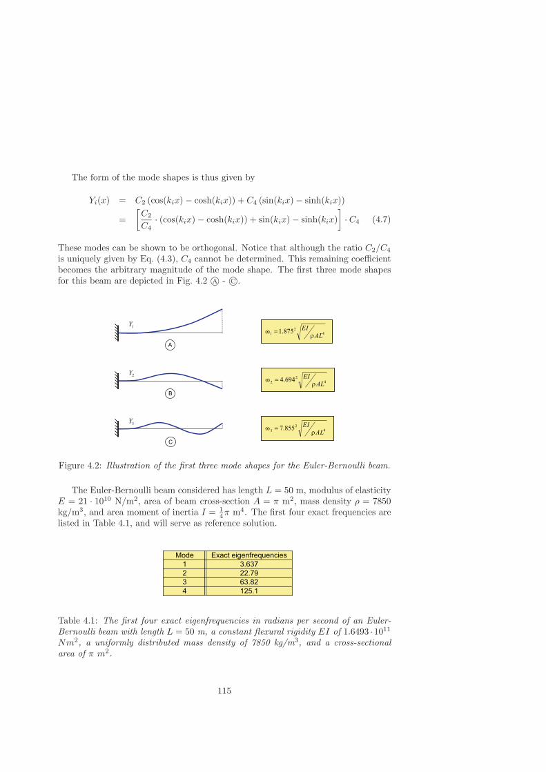
The form of the mode shapes is thus given by

Yi(x) = C2 (cos(kix) − cosh(kix)) + C4 (sin(kix) − sinh(kix))

=[C2

C4· (cos(kix) − cosh(kix)) + sin(kix) − sinh(kix)

]· C4 (4.7)

These modes can be shown to be orthogonal. Notice that although the ratio C2/C4

is uniquely given by Eq. (4.3), C4 cannot be determined. This remaining coefficientbecomes the arbitrary magnitude of the mode shape. The first three mode shapesfor this beam are depicted in Fig. 4.2 A© - C©.

Figure 4.2: Illustration of the first three mode shapes for the Euler-Bernoulli beam.

The Euler-Bernoulli beam considered has length L = 50 m, modulus of elasticityE = 21 · 1010 N/m2, area of beam cross-section A = π m2, mass density ρ = 7850kg/m3, and area moment of inertia I = 1

4π m4. The first four exact frequencies arelisted in Table 4.1, and will serve as reference solution.

Table 4.1: The first four exact eigenfrequencies in radians per second of an Euler-Bernoulli beam with length L = 50 m, a constant flexural rigidity EI of 1.6493 ·1011

Nm2, a uniformly distributed mass density of 7850 kg/m3, and a cross-sectionalarea of π m2.

115

Exact rotating eigenfrequencies

Now we will present exact solutions to the frequency equation for transverse vibra-tions of a rotating Euler-Bernoulli beam. The rotating beam is a particular caseof the prestressed beam, of which the practical importance is considerable in theanalysis of wind turbine rotor blades. It is a physical known fact that the eigenfre-quencies of a rotating beam raise due to the component of the centrifugal accelerationfield along the beam leading to an additional stiffening term. This effect is in theliterature known as “centrifugal stiffening”.

The non-dimensional frequency ratios for a variety of rotating beams can befound in Wright et al. [320]. We use the results for an Euler-Bernoulli beam whichare repeated in Table 4.2. The exact values can be derived from the non-dimensionalvalues listed in the table by applying the following transformation (see Van Wo-erkom [316]):

ωi =1p

√(ω∗

i )2 − (ηi)2 for i = 1, 2, · · · 5 (4.8)

where

p =

√ρAL4

EI(4.9)

and ρ the mass density of the material, A the cross-sectional area, L the length,E the modulus of elasticity, I the area moment of inertia of the beam, and η thedimensionless rotation rate.

Frequency ratios of an Euler-Bernoulli beam

η ω∗1 ω∗

2 ω∗3 ω∗

4 ω∗5

0.0 3.5160 22.0345 61.6972 120.9020 199.8601.0 3.6817 22.1810 61.6418 121.0510 200.0122.0 4.1373 22.6149 62.2732 121.4970 200.4673.0 4.7973 23.3203 62.9850 122.2360 201.2234.0 5.5850 24.2734 63.9668 123.2610 202.2275.0 6.4495 25.4461 65.2050 124.5660 203.6226.0 7.3604 26.8091 66.6840 126.1400 205.2537.0 8.2996 28.3341 68.3860 127.9720 207.1618.0 9.2568 29.9954 70.2930 130.0490 209.3389.0 10.2257 31.7705 72.3867 132.3580 211.77510.0 11.2023 33.6404 74.6493 134.8840 214.46111.0 12.1843 35.5890 77.0638 137.6140 217.38512.0 13.1702 37.6031 79.6145 140.5340 220.536

Table 4.2: Non-dimensional frequency ratios of an Euler-Bernoulli beam as functionof the dimensionless rotation rate η.

116

Superelement approximation

In this case, the Euler-Bernoulli beam has been modeled using a number of superele-ments. Again, the beam is built in at the base. The torsional spring constants foreach superelement are determined as follows:

cz1 = cz3 =2EIzLse

[Nm]

with E the modulus of elasticity, Iz the area moment of inertia, and Lse the lengthof the superelement which is, in turn, defined as

Lse =L

Nse

with L the length of the Euler-Bernoulli beam and Nse the number of superelementsthe beam is subdivided in.

The first four eigenfrequencies of the superelement approximation as function ofthe number of elements are listed in Table 4.3. The pattern is clear: dividing thebeam into more superelements produces more eigenfrequencies (of which only thefirst four are shown), and improves the accuracy (compare columns with exact valueslisted in Table 4.1). The limiting case being an infinite number of superelements ofwhich the eigenfrequencies equal to those of the exact solution.

Table 4.3: The first four eigenfrequencies in radians per second of the superelementapproximation as function of the number of superelements.

The exact analytical solution is used to evaluate the superelement approximation.In order to do so, the relative frequency errors are computed. This error is definedas:

Relative error =Approximated eigenfrequency

Exact eigenfrequency· 100 − 100 [%]

The relative errors for the first four eigenfrequencies of the superelement approxi-mation are plotted in Fig. 4.3 as function of the number of superelements. Someeigenfrequencies are smaller, and some are larger than in reality, while the errorsreach the indicated 1 % error bound rather fast.

It can be concluded that the superelement modeling method used to discritizethe Euler-Bernoulli beam represents a consistent approximation to the exact modelwith an approximation accuracy that increases with an increasing number of su-perelements.

117

0 1 2 3 4 5 6 7 8 9 10

−5

0

5

10

15

20

Nse

[−]

Rel

ativ

e er

ror

[%

]

+ 1%

− 1%1st

2nd

3rd

4th

Figure 4.3: The relative errors for the first four eigenfrequencies of the superelementapproximation as function of the number of superelements Nse with k = 1

2 (1 − 1√3).

Dashed-dotted lines: + 1% and - 1% error bound respectively.

In addition, the mode shapes become also better defined with an increasingnumber of superelements, since information on more locations along the beam isavailable. Fig. 4.4 compares the first four analytical undamped mode shapes of anEuler-Bernoulli beam with those of the superelement approximation. The modeshapes are plotted from x = 0 to the full beam length of L = 50 m. The comparisonshows that at least n superelements are required to accurately approximate the firstn analytical mode shapes of an Euler-Bernoulli beam.

Recall that the form of the analytical mode shapes is given by Eq. (4.7). Themode shapes of the superelement approximation are computed by extracting thestate-space matrices A: n × n state or system matrix, B: n × r input matrix, C:p × n output matrix, and D: p × r direct feedthrough matrix (with n number ofstates, r number of inputs, and p number of outputs) from the simulation model(i.e. Beam1sd, Beam2sd, Beam3sd and Beam4sd). For example, for Beam1sd n = 4,r = 1, and p = 1. Subsequently, the matrix eigenvalue problem is solved producinga diagonal matrix of generalized eigenvalues and a full matrix whose columns arethe corresponding eigenvectors.

Each column of the eigenvector matrix contains the stacked vector of local jointposition states (i.e. the angle of rotation of the 1 degree of freedom rotational jointexpressed in the body-local frame of reference) and local joint velocity states. Themodes are obtained by repeatedly picking an eigenvalue and selecting the associatedvector of local position states out of the eigenvector matrix. Subsequently, thevector of local position states is converted to global displacements using the pin jointlocations expressed in the Newtonian reference frame. Finally, the mode shapes are

118

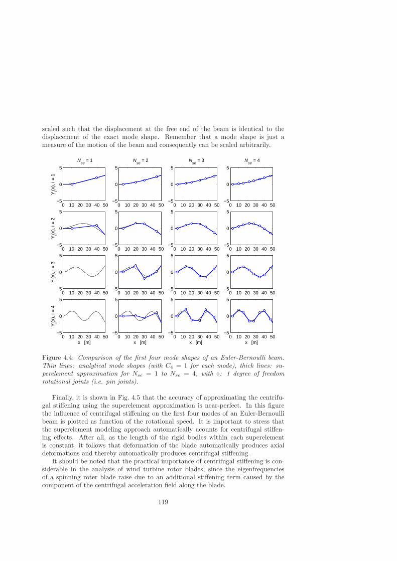
scaled such that the displacement at the free end of the beam is identical to thedisplacement of the exact mode shape. Remember that a mode shape is just ameasure of the motion of the beam and consequently can be scaled arbitrarily.

0 10 20 30 40 50−5

0

5

Nse

= 1

Yi(x

), i

= 1

0 10 20 30 40 50−5

0

5

Yi(x

), i

= 2

0 10 20 30 40 50−5

0

5

Yi(x

), i

= 3

0 10 20 30 40 50−5

0

5

Yi(x

), i

= 4

x [m]

0 10 20 30 40 50−5

0

5

Nse

= 2

0 10 20 30 40 50−5

0

5

0 10 20 30 40 50−5

0

5

0 10 20 30 40 50−5

0

5

x [m]

0 10 20 30 40 50−5

0

5

Nse

= 3

0 10 20 30 40 50−5

0

5

0 10 20 30 40 50−5

0

5

0 10 20 30 40 50−5

0

5

x [m]

0 10 20 30 40 50−5

0

5

Nse

= 4

0 10 20 30 40 50−5

0

5

0 10 20 30 40 50−5

0

5

0 10 20 30 40 50−5

0

5

x [m]

Figure 4.4: Comparison of the first four mode shapes of an Euler-Bernoulli beam.Thin lines: analytical mode shapes (with C4 = 1 for each mode), thick lines: su-perelement approximation for Nse = 1 to Nse = 4, with : 1 degree of freedomrotational joints (i.e. pin joints).

Finally, it is shown in Fig. 4.5 that the accuracy of approximating the centrifu-gal stiffening using the superelement approximation is near-perfect. In this figurethe influence of centrifugal stiffening on the first four modes of an Euler-Bernoullibeam is plotted as function of the rotational speed. It is important to stress thatthe superelement modeling approach automatically acounts for centrifugal stiffen-ing effects. After all, as the length of the rigid bodies within each superelementis constant, it follows that deformation of the blade automatically produces axialdeformations and thereby automatically produces centrifugal stiffening.

It should be noted that the practical importance of centrifugal stiffening is con-siderable in the analysis of wind turbine rotor blades, since the eigenfrequenciesof a spinning roter blade raise due to an additional stiffening term caused by thecomponent of the centrifugal acceleration field along the blade.

119

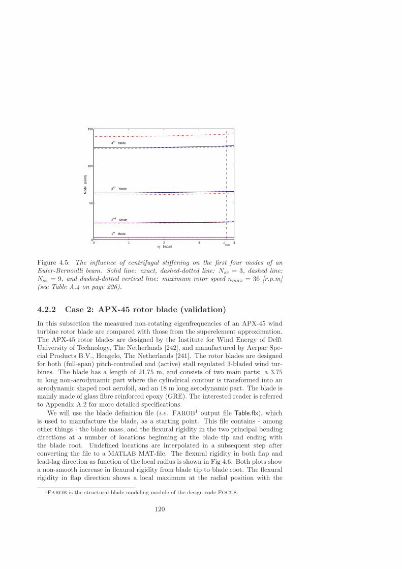
0 1 2 3 40

50

100

150

ωr [rad/s]

Mod

e [

rad/

s]

1st Mode

2nd Mode

3rd Mode

4th Mode

nmax

Figure 4.5: The influence of centrifugal stiffening on the first four modes of anEuler-Bernoulli beam. Solid line: exact, dashed-dotted line: Nse = 3, dashed line:Nse = 9, and dashed-dotted vertical line: maximum rotor speed nmax = 36 [r.p.m](see Table A.4 on page 226).

4.2.2 Case 2: APX-45 rotor blade (validation)

In this subsection the measured non-rotating eigenfrequencies of an APX-45 windturbine rotor blade are compared with those from the superelement approximation.The APX-45 rotor blades are designed by the Institute for Wind Energy of DelftUniversity of Technology, The Netherlands [242], and manufactured by Aerpac Spe-cial Products B.V., Hengelo, The Netherlands [241]. The rotor blades are designedfor both (full-span) pitch-controlled and (active) stall regulated 3-bladed wind tur-bines. The blade has a length of 21.75 m, and consists of two main parts: a 3.75m long non-aerodynamic part where the cylindrical contour is transformed into anaerodynamic shaped root aerofoil, and an 18 m long aerodynamic part. The blade ismainly made of glass fibre reinforced epoxy (GRE). The interested reader is referredto Appendix A.2 for more detailed specifications.

We will use the blade definition file (i.e. FAROB1 output file Table.flx), whichis used to manufacture the blade, as a starting point. This file contains - amongother things - the blade mass, and the flexural rigidity in the two principal bendingdirections at a number of locations beginning at the blade tip and ending withthe blade root. Undefined locations are interpolated in a subsequent step afterconverting the file to a MATLAB MAT-file. The flexural rigidity in both flap andlead-lag direction as function of the local radius is shown in Fig 4.6. Both plots showa non-smooth increase in flexural rigidity from blade tip to blade root. The flexuralrigidity in flap direction shows a local maximum at the radial position with the

1FAROB is the structural blade modeling module of the design code FOCUS.

120

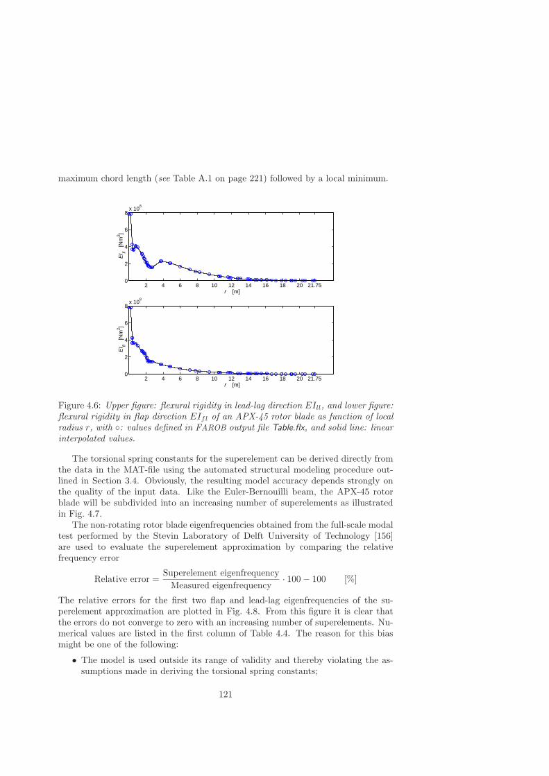
maximum chord length (see Table A.1 on page 221) followed by a local minimum.

2 4 6 8 10 12 14 16 18 20 21.750

2

4

6

8x 10

8

r [m]

EI ll

[Nm

2 ]

2 4 6 8 10 12 14 16 18 20 21.750

2

4

6

8x 10

8

r [m]

EI fl

[Nm

2 ]

Figure 4.6: Upper figure: flexural rigidity in lead-lag direction EIll, and lower figure:flexural rigidity in flap direction EIfl of an APX-45 rotor blade as function of localradius r, with : values defined in FAROB output file Table.flx, and solid line: linearinterpolated values.

The torsional spring constants for the superelement can be derived directly fromthe data in the MAT-file using the automated structural modeling procedure out-lined in Section 3.4. Obviously, the resulting model accuracy depends strongly onthe quality of the input data. Like the Euler-Bernouilli beam, the APX-45 rotorblade will be subdivided into an increasing number of superelements as illustratedin Fig. 4.7.

The non-rotating rotor blade eigenfrequencies obtained from the full-scale modaltest performed by the Stevin Laboratory of Delft University of Technology [156]are used to evaluate the superelement approximation by comparing the relativefrequency error

Relative error =Superelement eigenfrequency

Measured eigenfrequency· 100 − 100 [%]

The relative errors for the first two flap and lead-lag eigenfrequencies of the su-perelement approximation are plotted in Fig. 4.8. From this figure it is clear thatthe errors do not converge to zero with an increasing number of superelements. Nu-merical values are listed in the first column of Table 4.4. The reason for this biasmight be one of the following:

• The model is used outside its range of validity and thereby violating the as-sumptions made in deriving the torsional spring constants;

121

Figure 4.7: Schematic of the APX-45 rotor blade and its two superelement approxi-mation, with : 2 degrees of freedom rotational joints.

• The blade structural properties in reality differ from their designed values dueto uncertain material parameters and manufacturing tolerances. The APX-45rotor blades are produced by moulding processes using composite materialsof which the material properties are not known exactly. The upper and lowerblade surfaces are manufactured separately in two moulds by hand-lay-up, andjoined together using high strength adhesives. The result being that the blademass and blade dimension are not precisely controllable;

• Quality of the applied experiments and determination of the eigenfrequenciesfrom the measurements are not adequate. The natural frequencies of the APX-45 rotor blade have been determined from hand-excited displacement measure-ments in both lead-lag and flap direction. The displacements were measuredat two locations using LVDT’s (linear variable differential transducers);

• The flexibility of the test stand in which the blade has been mounted duringthe modal testing can not be neglected.

When the frequency errors for the first three flap and lead-lag eigenfrequenciesof the superelement approximation are calculated relative to the eigenfrequencies ascomputed by FAROB, they converge to zero. It should be noted that the FAROB

approximation also divides the blade in beam elements, but requires a significantlyhigher (> 100) number of elements. This illustrates (again) the power of the su-perelement approach.

Finally, the Finite Element program MARC [176] will be used to check whetherthe model assumptions are violated. The finite element mesh has been generatedusing the aforementioned blade definition file. The elements are eight noded, thickshell elements with 6 degrees of freedom at each node (MARC element type 22). The

122

1 2 3 4 5 6

−5

0

5

10

15

20

25

Nse

[−]

Err

or r

elat

ive

to S

L−D

UT

mea

sure

men

ts

[%]

+ 2%

− 2%

1st Flap

2nd Flap

1st Lead−Lag

2nd Lead−Lag

Figure 4.8: The relative errors for the first two flap and lead-lag non-rotating eigen-frequencies of the APX-45 rotor blade as function of the number of superelementsNse. Dashed-dotted horizontal lines: + 2% and - 2% error bound respectively.

elements have a composite layer structure. The layers of the composite are composedof orthotropic material. The total model contains 3137 elements, and 3055 nodesresulting in 18330 degrees of freedom. The first 15 eigenfrequencies were calculatedusing the Lanczos eigenvalue extraction algorithm. The resulting frequency errors ofthe first two flap and lead-lag eigenfrequencies of the APX-45 rotor blade are listedin the second column of Table 4.4.

APX-45 rotor blade

Difference Nse = 6 w.r.t. Difference MARC w.r.t.ModeSL-DUT measurements SL-DUT measurements

1st flap − 4.1% + 1.0%1st lead-lag − 2.6% − 9.1%

2 nd flap − 0.3% + 3.0%2 nd lead-lag − 2.8% − 12.6%

Table 4.4: Comparison of the first two flap and lead-lag non-rotating rotor bladeeigenfrequencies calculated using the superelement approximation for Nse = 6 (left)and MARC (right) to the ones from a full-scale modal test performed by the StevinLaboratory of Delft University of Technology (SL-DUT).

123

It can be concluded that the effect of violating the model assumptions is probablynegligible, but that the quality of the model is either limited by the quality of theinput, or by the quality of the applied experiments and resulting eigenfrequencydetermination. In the next subsection we will further investigate the cause of theobserved bias by examining an APX-70 rotor blade.

4.2.3 Case 3: APX-70 rotor blade (validation)

As discussed in the previous subsection, the relative frequency error is most likelyto be associated with the fact that the blades are manufactured by hand-lay-upand quality of the applied experiments and resulting eigenfrequency determination.In order to check those assumptions, the measured non-rotating eigenfrequencies ofan APX-70 wind turbine rotor blade are in this subsection compared with thosefrom the superelement approximation. The APX-70 rotor blade is suited for pitchcontrolled turbines with a rated power of 1.5 MW and is designed, and manufacturedby Aerpac Special Products B.V., Hengelo, The Netherlands [122].

The labour-intensive and inaccurate hand-lay-up manufacturing technique of theAPX-45 blades has been replaced by a resin-infusion moulding (RIM) technique.With RIM the glass cloth is laid dry into the mould which is subsequently coveredby plastic sheeting, sealed, and evacuated. The resin is then drawn in under thevacuum bag. Finally, the upper and lower blade surfaces are joined together usinghigh strength adhesives.

The natural frequencies of the APX-70 rotor blade have been determined fromhand-excited displacement measurements identical to those of the APX-45 blade[122], as well as by a more sophisticated modal analysis carried out by NetherlandsOrganization for Applied Scientific Research (TNO) [27]. In the latter case, boththe input force (generated by instrumented hammer excitation) and the resultingresponses are measured using a force transducer integrated in the hammer headand high-sensitivity accelerometers respectively. The blade was instrumented with8 accelerometers in lead-lag direction and 16 accelerometers in flap direction (onepositioned near the leading edge and one positioned near the trailing edge).

In the first column of Table 4.5 the eigenfrequencies determined from the hand-excited displacement measurements performed by the Stevin Laboratory (SL-DUT)are compared to the ones resulting from the modal analysis performed by TNOunder contract of Delft University of Technology. It can be concluded based onthe listed difference of maximum 1.8% that the combination of hand-excitationwith displacement measurements might be an explanation for the observed relativefrequency error in the APX-45 case.

The errors for the first three flap and first two lead-lag eigenfrequencies of theAPX-70 rotor blade are plotted relative to the TNO measurements as function of thenumber of superelements in Fig. 4.9. The bias of the first (− 3.9%) and second mode(− 1.8%) in flap direction are slightly larger than the ones observed in the APX-45 case. In lead-lag direction, however, the superelement approximation producessignificantly higher values for the eigenfrequencies (the bias of the first mode is11.0%, while the bias of the second mode is 17.5%).

124

APX-70 rotor blade

Difference SL-DUT w.r.t. Difference MARC w.r.t.ModeTNO measurements TNO (SL-DUT) measurements

1st flap + 1.8% − 0.2% (− 2.0%)1st lead-lag + 1.8% + 0.9% (− 0.9%)

2 nd flap − 1.3% + 1.4% (+ 2.7%)2 nd lead-lag + 1.2% + 6.6% (+ 5.3%)

3 rd flap + 0.0% + 2.6% (+ 2.6%)

Table 4.5: Comparison of eigenfrequencies determined from the displacement mea-surements performed by the Stevin Laboratory of Delft University of Technology (SL-DUT) to the ones resulting from the modal analysis performed by TNO (left) andcomparison of the eigenfrequencies calculated by MARC relative to both the TNO andSL-DUT measurements (right) [122].

1 2 3 4 5 6−10

0

10

20

30

40

50

Nse

[−]

Err

or r

elat

ive

to T

NO

mea

sure

men

ts

[%]

+ 2%

− 2%

1st Flap

2nd Flap

3rd Flap

1st Lead−Lag

2nd Lead−Lag

Figure 4.9: The relative errors for the first three flap and first two lead-lag eigenfre-quencies of the APX-70 rotor blade as function of the number of superelements Nse.Dashed-dotted horizontal lines: + 2% and - 2% error bound respectively.

Interestingly, the frequency errors of MARC with respect to either the TNO orthe SL-DUT measurements do not show the increased bias in lead-lag direction. Forthe purpose of illustration, the numerical values are listed in the second column ofTable 4.5 [313]. Clearly, this issue needs further research.

125

4.2.4 Case 4: RB-51 rotor blade (validation)

The Polymarin RB-51 rotor blade has been developed for wind turbines with arated power of 750 kW. The blade has a length of 24.20 m. The natural frequenciesof the RB-51 rotor blade have been determined from hand-excited displacementmeasurements carried out by the Stevin Laboratory (SL-DUT), as well as by a modalanalysis carried out by TNO under contract of Delft University of Technology [123].In the first column of Table 4.6 the resulting differences between the two methods arelisted. It can be concluded that the second lead-lag mode has the largest differenceand that the differences are larger than in the APX-70 case. The right columnshows the comparison of the eigenfrequencies calculated by MARC relative to boththe TNO and SL-DUT measurements.

RB-51 rotor blade

Difference SL-DUT w.r.t. Difference MARC w.r.t.ModeTNO measurements TNO (SL-DUT) measurements

1st flap + 2.4% − 0.2% (− 2.5%)1st lead-lag + 1.1% − 7.7% (− 8.7%)

2 nd flap + 2.8% + 3.2% (+ 0.5%)2 nd lead-lag + 6.1% − 0.7% (− 6.4%)

Table 4.6: Comparison of eigenfrequencies determined from the displacement mea-surements performed by the Stevin Laboratory of Delft University of Technology (SL-DUT) to the ones resulting from the modal analysis performed by TNO (left) andcomparison of the eigenfrequencies calculated by MARC relative to both the TNO andSL-DUT measurements (right) [123].

The errors for the first two flap and first two lead-lag eigenfrequencies of theRB-51 rotor blade are plotted relative to the TNO measurements as function of thenumber of superelements in Fig. 4.10. The most striking characteristic of this plotis that the final bias is already reached with only three superelements. For Nse = 6,the biases of the first mode in flap and lead-lag direction are 1.1% and −1.3%respectively, while the biases of the second modes in flap and lead-lag direction are8.1% and 8.0% respectively.

4.2.5 Case 5: RB-70 rotor blade (validation)

The RB-70 rotor blade has been developed by Polymarin for wind turbines measuring70 m in diameter with a rated power of 1.5 MW. The tested blade, however, hasa length of 28.75 m since a part of the tip has been removed [28]. The naturalfrequencies of this rotor blade have been determined from hand-excited displacementmeasurements carried out by the Stevin Laboratory (SL-DUT), as well as by a modal

126

1 2 3 4 5 6

−10

0

10

20

30

40

Nse

[−]

Err

or r

elat

ive

to T

NO

mea

sure

men

ts

[%]

+ 2%

− 2%

1st Flap

2nd Flap

1st Lead−Lag

2nd Lead−Lag

Figure 4.10: The relative errors for the first three flap and first two lead-lag eigenfre-quencies of the RB-51 rotor blade as function of the number of superelements Nse.Dashed-dotted horizontal lines: + 2% and - 2% error bound respectively.

analysis carried out by TNO under contract of Delft University of Technology [124].In the first column of Table 4.6 the resulting differences between the two methodsare listed. It can be concluded that the differences are small. The right columnshows the comparison of the eigenfrequencies calculated by MARC relative to boththe TNO and SL-DUT measurements. The prediction in flap direction is worse thanthe prediction in lead-lag direction.

RB-70 rotor blade

Difference SL-DUT w.r.t. Difference MARC w.r.t.ModeTNO measurements TNO (SL-DUT) measurements

1st flap − 1.4% + 6.2% (+ 7.7%)1st lead-lag + 1.2% − 4.3% (− 5.5%)

2 nd flap + 0.2% + 12.5% (+ 12.3%)2 nd lead-lag + 0.6% − 1.5% (− 2.1%)

Table 4.7: Comparison of eigenfrequencies determined from the displacement mea-surements performed by the Stevin Laboratory of Delft University of Technology (SL-DUT) to the ones resulting from the modal analysis performed by TNO (left) andcomparison of the eigenfrequencies calculated by MARC relative to both the TNO andSL-DUT measurements (right) [124].

127

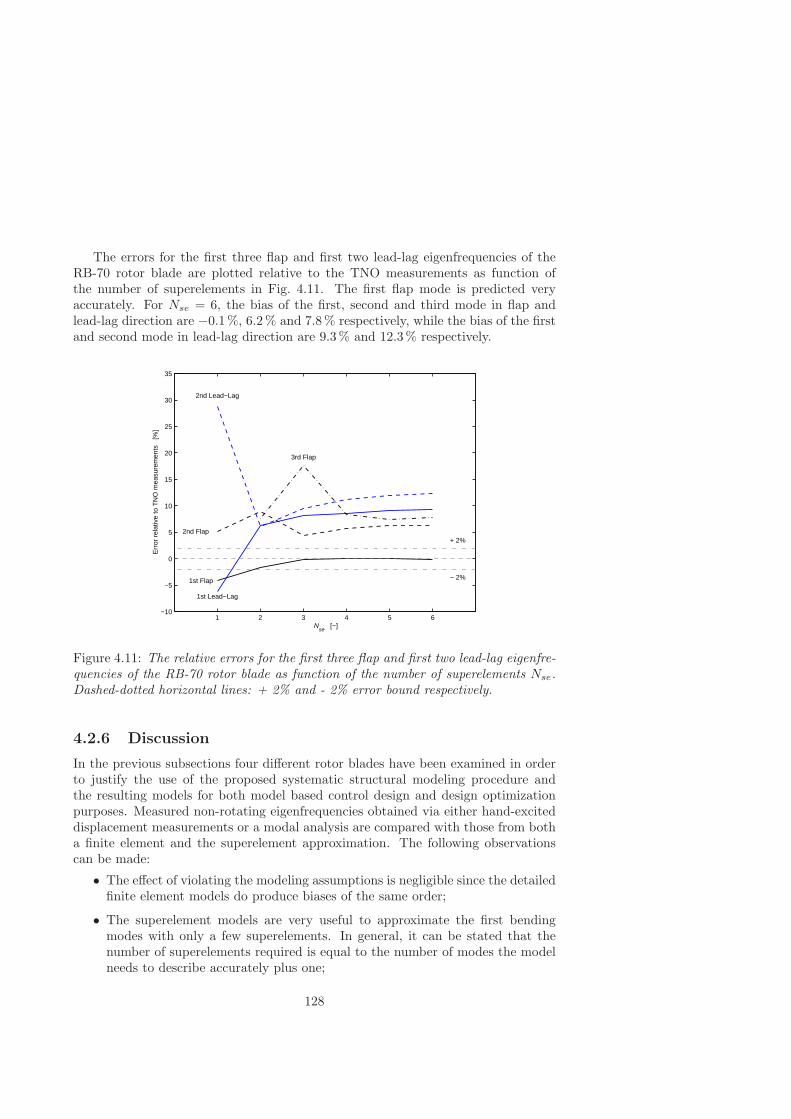
The errors for the first three flap and first two lead-lag eigenfrequencies of theRB-70 rotor blade are plotted relative to the TNO measurements as function ofthe number of superelements in Fig. 4.11. The first flap mode is predicted veryaccurately. For Nse = 6, the bias of the first, second and third mode in flap andlead-lag direction are −0.1%, 6.2% and 7.8% respectively, while the bias of the firstand second mode in lead-lag direction are 9.3% and 12.3% respectively.

1 2 3 4 5 6−10

−5

0

5

10

15

20

25

30

35

Nse

[−]

Err

or r

elat

ive

to T

NO

mea

sure

men

ts

[%]

+ 2%

− 2%1st Flap

2nd Flap

3rd Flap

1st Lead−Lag

2nd Lead−Lag

Figure 4.11: The relative errors for the first three flap and first two lead-lag eigenfre-quencies of the RB-70 rotor blade as function of the number of superelements Nse.Dashed-dotted horizontal lines: + 2% and - 2% error bound respectively.

4.2.6 Discussion

In the previous subsections four different rotor blades have been examined in orderto justify the use of the proposed systematic structural modeling procedure andthe resulting models for both model based control design and design optimizationpurposes. Measured non-rotating eigenfrequencies obtained via either hand-exciteddisplacement measurements or a modal analysis are compared with those from botha finite element and the superelement approximation. The following observationscan be made:

• The effect of violating the modeling assumptions is negligible since the detailedfinite element models do produce biases of the same order;

• The superelement models are very useful to approximate the first bendingmodes with only a few superelements. In general, it can be stated that thenumber of superelements required is equal to the number of modes the modelneeds to describe accurately plus one;

128

• The difference between the hand-lay-up (APX-45) and resin-infusion moulding(RIM) manufacturing technique (APX-70) could not be detected since thesupplied mass distribution was already modified to diminish the differencebetween the measured and simulated mass and center of gravity location;

• The model accuracy is strongly limited by the quality of the supplied inputdata.

To stress the importance of the latter observation, we have used measured dis-placement information of static tests applied to both the APX-70 and the RB-70rotor blade to modify the torsional spring constants accordingly. The displacementis measured using a LVDT located at a radial position of r = 26.75 m (APX-70) andr = 26.2 m (RB-70). The torsional springs of the APX-70 blade in flap directionare increased with 8.6 % and in lead-lag direction reduced with 24.4 %, while thethe torsional springs of the RB-70 blade are reduced in flap direction with 0.6 %and in lead-lag direction reduced with 18.5 %. The results are plotted in Fig. 4.12for Nse = 1, · · · , 6, while for Nse = 6 the numerical values are listed in Table 4.8.The upper figure shows the relative frequency errors of the APX-70 blade, while thelower figure shows the errors of the RB-70 blade.

1 2 3 4 5 6

−10

0

10

20

30

Nse

[−]

APX−70 rotor blade (modified)

Err

or r

elat

ive

to T

NO

mea

sure

men

ts

[%]

+ 2%

− 2%1st Flap

2nd Flap

3rd Flap

1st Lead−Lag

2nd Lead−Lag

1 2 3 4 5 6−20

−10

0

10

20

Nse

[−]

RB−70 rotor blade (modified)

Err

or r

elat

ive

to T

NO

mea

sure

men

ts

[%]

+ 2%

− 2%1st Flap

2nd Flap

3rd Flap

1st Lead−Lag

2nd Lead−Lag

Figure 4.12: The relative errors for the first three flap and first two lead-lag eigen-frequencies of the APX-70 rotor blade (upper plot) and RB-70 rotor blade (lowerplot) as function of the number of superelements Nse. Displacement informationof static tests has been used to modify the torsional spring constants accordingly.Dashed-dotted horizontal lines: + 2% and - 2% error bound respectively.

It can be concluded by comparing the modified and original frequency error valuesfor Nse = 6 listed in Table 4.8 that adding measured displacement information (even

129

at only one location) significantly reduces the absolute frequency error value. Themean value of the absolute frequency error is reduced from 7.2 % to 2.9 % in theAPX-70 case, while for the RB-70 blade this value is reduced from 7.1 % to 3.3 %.It is expected that an even higher accuracy can be obtained if displacement (oracceleration) information is available at more radial positions. After all, this offersthe possibility to tune the torsional spring constants individually using the proceduretreated in Chapter 5.

Modified APX-70 and RB-70 rotor blade

Difference Nse = 6 w.r.t. Difference Nse = 6 w.r.t.ModeTNO measurements TNO measurements

1st flap + 0.1% (− 3.9%) − 0.4% (− 0.1%)1st lead-lag − 3.5% (+ 11.0%) − 1.3% (+ 9.3%)

2 nd flap + 2.3% (− 1.8%) + 5.9% (+ 6.2%)2 nd lead-lag + 2.2% (+ 17.5%) + 1.3% (+ 12.3%)

3 rd flap + 6.3% (+ 2.0%) + 7.5% (+ 7.8%)

Table 4.8: Comparison of APX-70 and RB-70 rotor blade non-rotating eigenfre-quencies calculated using the superelement approximation with modified (original)torsional spring constants for Nse = 6 to the ones resulting from the modal analysisperformed by TNO.

In the previous six cases the validity of the proposed systematic structural mod-eling procedure has been examined. We felt that it was important first to verifythe proposed systematic structural modeling procedure using a test case, and sub-sequently to validate the approach using individual modal tests carried out on anumber of rotor blades before applying it to a complete flexible wind turbine.

The test case shows that the superelement modeling method represents a consis-tent approximation to the Euler-Bernouilli beam with an approximation accuracythat increases with an increasing number of superelements. Furthermore, we founda good agreement between the measured non-rotating eigenfrequencies of variouswind turbine rotor blades and those calculated using the superelement approxima-tion. This means that the mass and stiffness properties of the rotor blade modelsare appropriate.

The aforementioned results demonstrate that it is, in principle, possible to de-rive limited order multibody models suited for time-domain simulation, analysis ofdynamic loads, and model based control design directly from physical rotor blade de-sign data using the proposed systematic structural modeling procedure. Dependingon the intended model use, tuning of torsional spring constants using either statictest data or experimental modal test data is required to reach the desired accuracy.We will now continue the validation using data acquired from a full-scale modal testapplied to the Lagerwey LW-50/750 wind turbine.

130

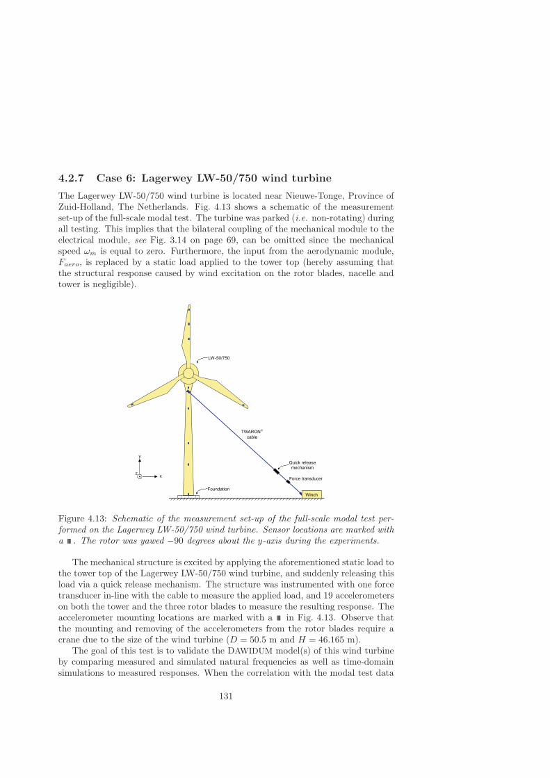
4.2.7 Case 6: Lagerwey LW-50/750 wind turbine

The Lagerwey LW-50/750 wind turbine is located near Nieuwe-Tonge, Province ofZuid-Holland, The Netherlands. Fig. 4.13 shows a schematic of the measurementset-up of the full-scale modal test. The turbine was parked (i.e. non-rotating) duringall testing. This implies that the bilateral coupling of the mechanical module to theelectrical module, see Fig. 3.14 on page 69, can be omitted since the mechanicalspeed ωm is equal to zero. Furthermore, the input from the aerodynamic module,Faero, is replaced by a static load applied to the tower top (hereby assuming thatthe structural response caused by wind excitation on the rotor blades, nacelle andtower is negligible).

Figure 4.13: Schematic of the measurement set-up of the full-scale modal test per-formed on the Lagerwey LW-50/750 wind turbine. Sensor locations are marked witha . The rotor was yawed −90 degrees about the y-axis during the experiments.

The mechanical structure is excited by applying the aforementioned static load tothe tower top of the Lagerwey LW-50/750 wind turbine, and suddenly releasing thisload via a quick release mechanism. The structure was instrumented with one forcetransducer in-line with the cable to measure the applied load, and 19 accelerometerson both the tower and the three rotor blades to measure the resulting response. Theaccelerometer mounting locations are marked with a in Fig. 4.13. Observe thatthe mounting and removing of the accelerometers from the rotor blades require acrane due to the size of the wind turbine (D = 50.5 m and H = 46.165 m).

The goal of this test is to validate the DAWIDUM model(s) of this wind turbineby comparing measured and simulated natural frequencies as well as time-domainsimulations to measured responses. When the correlation with the modal test data

131

is not satisfactory, the time domain data can be used to update (some of) the modelparameters following the approach that will be presented in Chapter 5. In the nextparagraphs the applied excitation technique, the performed pre-test analysis as wellas the results will be discussed in detail.

Excitation using step-relaxation

In principle two main ways to excite a structure, viz. ambient excitation and exter-nally forced excitation:

• Ambient excitation. Ambient excitation implies that the structure is testedin situ, using the operational vibrations as the excitation source. Examplesare traffic in the case of bridges or wind in the case of wind turbines. Ambientexcitation is frequently used to excite large structures where externally forcedexcitation becomes difficult, inconvenient and/or expensive. For example, windexcitation has been applied to extract the modal parameters of the 110-m-tall EOLE vertical-axis wind turbine [40] and has been used to validate anADAMS/WT model of the Cannon Wind Eagle 300 downwind horizontal-axiswind turbine [134, 319];

• Externally forced excitation. In this case both the input force and theresulting responses are measured. The input forces may be generated in severalways (i.e. electromagnetic or hydraulic shaker, instrumented hammer, humanexcitation or step relaxation).

The preferred exciter is often the electromagnetic shaker which has the ability, whenproperly sized, to provide a flexible way of specifying sufficiently exciting inputs.Conversely, for parked wind turbine testing, human excitation, step relaxation, andwind excitation are the most useful [152]. Human excitation, however, is limitedto moderately sized wind turbines, because small turbines have natural frequenciestoo high to be excited manually, while larger turbines may be too massive to excite.Step relaxation as well as wind excitation have been reported to work extremely wellon vertical-axis wind turbines [40, 151, 152]. Of the two excitation techniques, steprelaxation is the most time-consuming. However, the frequency content of the stepfunction makes it ideal for testing large, flexible structures since a large amount ofstrain energy can be input to the structure. In addition, it has been observed thatstructural damping is difficult to estimate accurately from the measurements usingwind excitation.

We have decided to use the step-relaxation method to excite the parked Lager-wey LW-50/750 wind turbine because its ability to estimate the damping and thefact that it is mechanically straightforward to implement. This method of structuralexcitation involves applying a static load to the structure by a cable anchored to theground or to a deadweight, and then suddenly releasing this load via a quick releasemechanism. The static load was transmitted by a 225 meter long TWARON R© cable.TWARON is a lightweight, superstrong synthetic fibre made from the aramid poly-mer. It is preferred to steel because it is five times lighter at the same strength (thecable has a tensile strength of 170 kN and a total mass of 82.5 kg). The interested

132

reader is referred to Appendix F.1 for a more detailed technical specification of thecable. Consequently, the mass loading is minimized. The only disadvantage is thelower modulus of elasticity, which is about half that of steel [47]. The cable has beensecured to the tower at 40.5 m above the ground level using a cargo strap. A cargostrap was preferred to a fixture because mass loading is negligible and no specialfixturing is required.

We have used a 20-ton truck as deadweight and used its hydraulic powered winchfor loading the cable to the specified 40 kN. The tension in the cable is released bya firm pull on a nylon cord that activates the lever switch of the quick releasemechanism. The cable is restrained at both ends by a chain preventing secondaryhits or random banging after being released.

The left photograph in Figure 4.14 shows the initial position of the TWARON R©

cable, quick release mechanism, nylon cord, chain, force transducer, and the winchcable. The middle and right photograph show two successive frames of an actualrelease recorded with a Mini DV camera.

Figure 4.14: Step-relaxation hardware and recorded release. Left photograph: positionof the TWARON cable, quick release mechanism, nylon cord, chain, force transducer,and winch cable at T = 0.0 s, middle photograph: position at T = 0.08 s, and rightphotograph: position at T = 0.16 s.

Pre-test analysis

Pre-test analysis was performed on two DAWIDUM models, notably SDLW1: an 18-DOF model, and SDLW2: a 34-DOF model. Both models describe the structuraldynamics of the complete Lagerwey LW-50/750 wind turbine (see Appendix I.2.3for more details). The analysis results have been used to determine the frequencyrange of interest, the required input force magnitude, the driving point on the tower,and the accelerometer locations:

• Frequency range of interest. From a dynamic analysis performed on theaforementioned DAWIDUM models it can be concluded that the dynamic re-sponse of the Lagerwey LW-50/750 wind turbine is dominated by the firstfew bending modes. These modes are in the frequency range of 0.5 to 40Hz. Because of this low frequency range combined with light damping, eachtime record requires a duration of at least one minute. We selected a cutofffrequency of 160 Hz for the antialiasing filters and a sample frequency of 500

133

Hz for the measured signals. This choice is based on the above mentionedfrequency range of interest, the requirement to be able to accurately estimatestructural damping, and the fact that the number of data points of the useddata acquisition system (SCADAS II of Leuven Measurement Systems), is lim-ited to 32768 points. The interested reader is referred to Appendix F.2 wheredetailed specifications of the SCADAS II can be found;

• Input force. Obviously, the applied input force must cause no damage tothe Lagerwey LW-50/750 wind turbine. Conversely, the input force should besufficiently exciting to ensure that the responses contain sufficient informationin the frequency range of interest. On the basis of simulations performed onthe SDLW1 model it turned out that a 40 kN force should be adequate.

A force transducer was placed in-line with the cable between the quick releasemechanism and the winch truck to measure the input force. Although it isimportant for the force transducer to be close to the turbine so that it sensesthe force actually being applied to the structure [151], we have decided toplace the force transducer close to the winch truck to avoid collision of thetransducer with the tower;

• Accelerometer locations. Uniaxial accelerometers were used to measure theresponse at a number of locations on the tower as well as rotor blades. Theaccelerometers were placed on the blades so that they measured either purelylead-lag or flap deformations. The accelerometer mounting locations wereselected on the basis of simulations performed on the SDLW1 module in orderto avoid that an accelerometer is placed at a node for a frequency of interest.During instrumentation, however, it turned out that the crane was not able toreach the required working height of 75 meter. Consequently, we were forcedto slightly adapt both the instrumentation procedure and the accelerometermounting locations. In Appendix F.4 the final mounting locations as well asthe technical specifications of the accelerometers are listed.

It can be concluded that the mass of the accelerometers (28 grams (rotorblade) and 46 grams (tower) respectively) is negligible compared to the bladeand tower mass. Prior to mounting the accelerometers, both the tower androtor blade surface were cleaned. The accelerometers mounted on the bladesare bond in place with hot glue for easy attachment and removal. The toweraccelerometers are mounted using double-back tape. Response measurementswere made normal to the blade and tower.

Because this turbine has low natural frequencies, the acceleration responsewill be low. Also the transducer cables were quite long (ranging from 10 to 85meter), making noise a special consideration. To address this problem, veryhigh ly sensitive accelerometers with low-noise cables were used. All signalswere low-pass filtered using analogue filters to avoid aliasing.

134

Experiments

Prior to the experiments, the results from the pre-test analysis are checked by per-forming an initial test which has not been recorded. This test has also been used toobtain adequate accelerometer response levels to minimize the quantisation errorsas well as to determine an appropriate total experiment time / sample frequencycombination. The input force was applied under an angle α of 10.1 degrees withthe horizontal (see Figure 4.14). That is, the component of the force in positivex-direction is equal to Fx = Fcable ·cosα, and the component of the force in negativey-direction is equal to Fy = Fcable · sinα.

The main specifications of the recorded experiments are listed in Table 4.9. Allmeasurements have been preceded by a pre-trigger time of at least 0.240 s (the pre-trigger time varies with the quickness of response of the quick release mechanismoperator). It should be stressed that all testing was done in very low winds (lessthan 3 m/s at the tower top).

Table 4.9: Modal analysis measurement overview: main specifications of the recordedexperiments.

The signals of the first measurement (i.e. M1) are sampled with a sample fre-quency of 1000 Hz, while the signals of measurements M2-M10 are sampled with asample frequency of 500 Hz. The cutoff frequency of the ETD (equal time delay)anti-aliasing filter was set to 330 and 160 Hz respectively. From the Bode diagramof this filter (see Fig. F.3 on page 249) it can be concluded that the measured re-sponses are undistorted up to and including 0.15 · fco. This implies that if usefulinformation is contained in frequencies above 24 Hz (measurement M1) or 49.5 Hz(measurements M2-M10) it might be distorted and should be handled with care.However, since the anti-aliasing filter is known, it can be included as a known partof the model and let the simulated acceleration responses pass through this filterbefore being compared to the measured responses.

It should be mentioned that we had planned more experiments than listed inTable 4.9 (including an experiment with a 180 yawed rotor position, and one wherethe pitch angles of all three rotor blades are set to 45). However, the adapted in-strumentation procedure took up a lot more time than planned and we were forcedto limit ourselves to the most important experiments. The planned and the actualduration of the instrumentation, measurements and removal are compared in Ta-ble 4.10. The parked modal test of the Lagerwey LW-50/750 wind turbine requiredthe effort of at least 8 people in one day.

135

Table 4.10: Time schedule full-scale modal test performed on the Lagerwey LW-50/750 wind turbine.

Time series analysis

Figure 4.15 shows a typical tower top acceleration response in x-direction (i.e. sen-sor A-05) from a parked modal test. Obviously, the stepwise change in the forceapplied to the tower top excites a wide range of natural frequencies. The relativehigh frequencies at the beginning of the response are damped out quickly, leavingeventually the single frequency associated with the lowest system mode of vibra-tion. This mode is in literature often denoted with the misleading term “first towerbending mode”. The main reason for the domination of the response by the lowestsystem mode of vibration is that the total mass of the generator, chassis and rotoris relatively large with respect to the tower mass.

−10 0 10 20 30 40 50 60 70−5

0

5

Time [s]

A−

05

[m/s

2 ]

5 10 15 20 25 30 35−0.5

0

0.5

Time [s]

A−

05

[m/s

2 ]

Figure 4.15: Measured tower top acceleration (sensor A-05) from measurement M2.Upper figure: complete signal, and lower figure: zoom from 5 to 35 seconds.

The response in Figure 4.15 also shows that the record length is not long enoughto capture the complete response history. When the truncated time-domain responseis transformed into the frequency domain using the Fast Fourier Transform (FFT)

136

this may result in so-called leakage errors. In this case the distortion due to leakageis negligible because the truncated response contains only one mode and this modeis truly periodic in time.

The corresponding periodogram estimate of the power spectral density (PSD)is depicted in Fig. 4.16. It shows how the average power of the tower top accel-eration response in x-direction is distributed with frequency. The PSD estimateis computed via the Thomson multitaper method, and has a frequency resolutionof 500/32768 = 0.0153 Hz. Prior to the computation of the PSD, the accelera-tion record was pre-processed by filtering the data without phase distortion with aneighth order lowpass digital Butterworth filter with a cutoff frequency of 125 Hz,and subsequently removing the linear trend. It is clear that noise is not the primaryproblem since the individual peaks indicating the modes are clearly discernible inthe plot.

Integrating the total area under the curve reveals that 99% of the average poweris located below 102.7 Hz (73.6% of the average power is contained in the first systemmode of vibration, 5.2% in the fourth system mode, and 0.7% in the fifth systemmode). This average power distribution confirms the domination of the first systemmode of vibration in the time-domain response.

0 5 10 15 20 25 30 35 400

0.1

0.2

0.3

Frequency [Hz]

Pow

er S

pect

ral D

ensi

ty

[Pow

er/H

z]

PSD of sensor A−05

0 5 10 15 20 250

5

10

15x 10

−3

Frequency [Hz]

Pow

er S

pect

ral D

ensi

ty

[Pow

er/H

z]

0.51

Hz

3.75

Hz

5.23

Hz

Figure 4.16: Periodogram estimate of the power spectral density (PSD) of the towertop acceleration (sensor A-05) from measurement M2. Upper figure: signal in thefrequency range of 0 to 40 Hz, and lower figure: zoomed in on the second bendingmode and higher.

The periodogram estimate of the PSD of both sensor A-03 and A-16, depicted inupper and lower part of Fig. 4.17 respectively, show a completely different picture.The top figure reveals that both the first and the fourth system mode in x-direction

137

(second and third mode are not present in this response) dominate the response ofsensor A-03 (located about halfway between the tower bottom and top, see Table F.1on page 251). Integrating the total area under the curve reveals that 22.6% of theaverage power is contained in the first system mode, 29.7% in the fourth systemmode, and 12.3% in the fifth system mode. The bottom figure reveals that theresponse of sensor A-16 is dominated by the fourth system mode of vibration inx-direction (the third system mode is not present in this response). Integrating thetotal area under the curve reveals that 4.3% of the average power is contained inthe first system mode, 7.6% in the second system mode, 0.5% in the third systemmode, 66.1% in the fourth system mode, and 27.8% in the fifth system mode.

0 5 10 15 20 25 30 35 400

5

10

15x 10

−3

Frequency [Hz]

Pow

er S

pect

ral D

ensi

ty

[Pow

er/H

z]

PSD of sensor A−03

0 5 10 15 20 25 30 35 400

0.5

1

1.5

2

2.5

Frequency [Hz]

Pow

er S

pect

ral D

ensi

ty

[Pow

er/H

z]

PSD of sensor A−16

Figure 4.17: Periodogram estimate of the power spectral density (PSD) of sensorA-03 (upper figure) and A-16 (lower figure) from measurement M2.

Fig. 4.18 shows the periodogram estimates of the PSD of the responses in x-direction as a function of the sensor position with respect to the ground level. Thisthree-dimensional plot reveals how the average power distribution changes with thesensor location. It shows that the modes of the Lagerwey LW-50/750 wind turbinein x-direction are not closely spaced, and not heavily damped. This implies thatthe modes are lightly coupled. Consequently, the turbine behaves at resonancepredominantly as a single-degree-of-freedom (SDOF) system: the structural responseat a natural frequency is (almost) completely determined by that mode.

Fig. 4.19 shows a two-dimensional view of Fig. 4.18. The viewpoint is set alongthe x-axis thereby disregarding the accelerometer position information. This figureclearly reveals that the dynamic response of the Lagerwey LW-50/750 wind turbinein x-direction is dominated by the first five bending modes. It should be stressedthat the geometrical complexity of the mode shapes, rather than the number ofmodes observed, determines the number of degrees of freedom.

138

Natural frequencies

The SDLW1 model of the Lagerwey LW-50/750 wind turbine is linearized and sub-sequently the matrix eigenvalue problem is solved producing the simulated naturalfrequencies. The first five measured and simulated natural frequencies are comparedin Table 4.11. It must be noted that the foundation spring stiffness of the SDLW1model has been tuned (35 % lower than the value provided by Lagerwey) to ensurethat the simulated initial tower top deflection equals the measured one. From thistable it can be concluded that the differences in natural frequency are small.

LW-50/750 turbine

Difference SDLW1Modew.r.t. measurements

1st 0.0%2nd + 5.7%3 rd 0.0%4 th + 5.3%5 th + 5.9%

Table 4.11: Comparison of simulated natural frequencies (SDLW1 model) to the onesresulting from the modal analysis applied to the Lagerwey LW-50/750.

Time-domain responses

In Fig. 4.20 and 4.21 the measured and simulated tower top acceleration response inx-direction are compared. To ensure that the simulation starts in steady-state, theequilibrium point has been determined, and the corresponding state vector has beensaved. This state vector is used as initial condition in the performed simulation.From the figures it is clear that the SDLW1 model accurately describes the realresponse. Note that the time-domain response depends on the unknown (viscous)damper constants. These constants have been estimated from the measured responseand are used to generate the presented time histories. To achieve (even) bettercorrelation with the measured response, all model parameters can be updated usingthe approach presented in Molenaar [191].

139

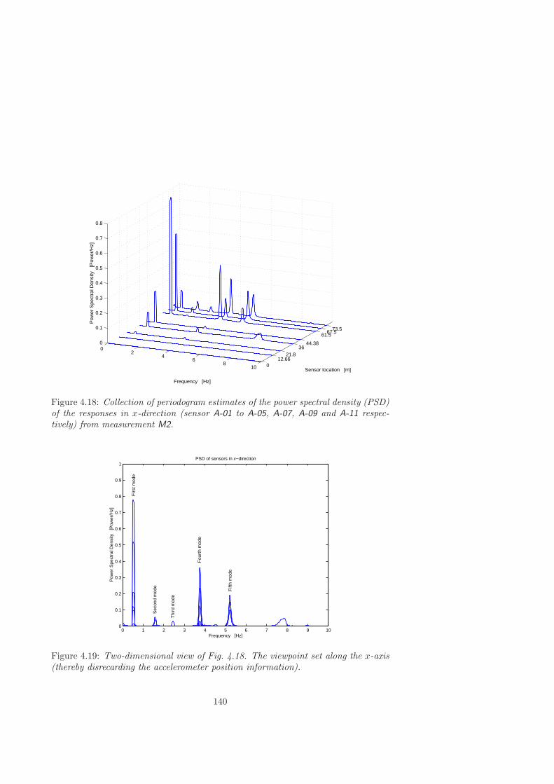
012.66

21.836

44.38

61.567.5

73.5

02

46

810

0

0.1

0.2

0.3

0.4

0.5

0.6

0.7

0.8

Sensor location [m]

Frequency [Hz]

Pow

er S

pect

ral D

ensi

ty

[Pow

er/H

z]

Figure 4.18: Collection of periodogram estimates of the power spectral density (PSD)of the responses in x-direction (sensor A-01 to A-05, A-07, A-09 and A-11 respec-tively) from measurement M2.

0 1 2 3 4 5 6 7 8 9 100

0.1

0.2

0.3

0.4

0.5

0.6

0.7

0.8

0.9

1PSD of sensors in x−direction

Frequency [Hz]

Pow

er S

pect

ral D

ensi

ty

[Pow

er/H

z]

Firs

t mod

e

Sec

ond

mod

e

Thi

rd m

ode

Fift

h m

ode

Fou

rth

mod

e

Figure 4.19: Two-dimensional view of Fig. 4.18. The viewpoint set along the x-axis(thereby disrecarding the accelerometer position information).

140

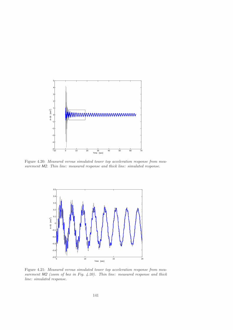
−10 0 10 20 30 40 50 60 70−5

−4

−3

−2

−1

0

1

2

3

4

5

Time [sec]

A−

05

[m/s

2 ]

Figure 4.20: Measured versus simulated tower top acceleration response from mea-surement M2. Thin line: measured response and thick line: simulated response.

5 10 15 20−0.5

−0.4

−0.3

−0.2

−0.1

0

0.1

0.2

0.3

0.4

0.5

Time [sec]

A−

05

[m/s

2 ]

Figure 4.21: Measured versus simulated tower top acceleration response from mea-surement M2 (zoom of box in Fig. 4.20). Thin line: measured response and thickline: simulated response.

141

4.3 Electrical module verification and validation

In this section the electrical module will be validated to justify the use of this modelfor model based control design purposes. First, a brief review of the existing liter-ature on synchronous machine identification and parameter determination is given.Next, a new procedure is developed (using ideas from Touhami et al. [291]) foridentifying the transfer functions of Park’s dq-axis model of a synchronous gener-ator from time-domain standstill step-response data. This procedure is applied tothe synchronous generator implemented in the Lagerwey LW-50/750 wind turbine.The validity of the theoretical model will been verified by comparing time-domainsimulations with measurements taken from the Lagerwey LW-50/750 generator.

4.3.1 Literature review

The design of a robust frequency converter controller for high dynamic performancerequires that the (synchronous) generator model parameters are known accurately.In principle, synchronous machine parameters may be determined either from designcalculations or from measurements acquired at the factory or on site. For high dy-namic performance control, however, the former approach is inadequate. A primarygoal of this section is to address the latter issue.

Many papers have been published on synchronous machine parameter identifi-cation (see e.g. [18, 136, 153, 248, 291, 294] and references therein). Most papersaddress standstill frequency response (SSFR) methods following the protocols ofIEEE Standard 115-1995 [111]. This standard focusses on identifying equivalentcircuit parameters rather than on transfer functions. Two papers address methodsfor identifying the parameters from time-domain data. In both cases, the param-eter estimation process generally consists of two parts. First, the time constantsare extracted by applying a curve-fitting procedure to measured data. Next, theequivalent circuit parameters are determined by solving a set of non-linear equa-tions through numerical optimization. The weakness of this approach is that theorder of the model must be known a priori and that numerical optimization is aprocess fraught with numerical difficulties [104].

4.3.2 Synchronous generator parameter identification

Synchronous machine identification and parameter determination can be performedeither during normal operation (i.e. on-line), or during specially designed identi-fication experiments (i.e. off-line) [90]. Each approach has advantages as well asdisadvantages. For example, in the on-line case the measured input-output datareflect the actual operating conditions. A disadvantage is that it is not possible tomanipulate the input signals arbitrarily in order to obtain the best identificationresults. This implies that the influence of the operating conditions on the (accuracyof the) identified parameters has to be carefully analysed. Off-line tests, on the otherhand, require that the machine under test has to be taken out of regular operation,an action that might be inappropriate or even impossible.

142

Off-line identification experiments have been used for decades to identify elec-trical machine parameters. Two concepts are commonly used: running machine,or standstill. Standstill tests are very attractive from a practical viewpoint - if itis permissible to take the machine out of operation - because driving the machineoften creates serious complications of the measurement set-up [301]. Furthermore,the measured signals will have good signal-to-noise ratios due to the absence ofdisturbance signals (electromagnetic interference). All standstill tests reported inliterature are variations on the same concept, they mainly differ in the kind of exci-tation signal applied (i.e. step, ramp, sinusoidal, or random excitation).

The standstill test concept is preferred because there is no interaction between thedirect- and the quadrature axis. Observe that the block diagram of Fig. 3.26 reducesto that of Fig. 4.22 for the standstill case (i.e. ωm = 0). Using this observation,it can be concluded that the parameter identification for both axes may be carriedout separately. In practice, zero generator speed can be enforced by mechanicallylocking the rotor during the experiments.

Figure 4.22: Block diagram of an ideal synchronous machine at standstill.

In addition, there are a few important practical demands in selecting a techniquefor the identification and parameter determination of the Lagerwey LW-50/750 gen-erator considering the fact that the generator has already been installed in the nacelleat about 50 meter above the ground level. First of all, the measurements shouldhave low power consumption. Secondly, the test equipment should be compact, andfinally, the measurement time should be limited (i.e. < 1 day).

143

Before selecting the most appropriate standstill test, we will first highlight themost important aspects of both the quadrature-axis and the direct-axis identifica-tion.

Quadrature-axis identification

The dynamic behavior of the quadrature-axis of an ideal synchronous generator isfully described by the transfer function Yq(s) in Fig. 4.22. From the block diagramit directly follows that

Yq(s) = − Iq(s)Uq(s)

=1

Rs + s · Lq(s)(4.10)

For the identification of Yq(s) knowledge of the quadrature-axis voltage uq(t) andcurrent iq(t) is thus both necessary and sufficient. It will be shown below that thesequantities can be easily derived from three measurable variables, viz. the statorvoltages of the b and c phase (ub(t), and uc(t) respectively), and the stator currentic(t).

An appropriate rotor position for quadrature-axis identification is the one whenthe field winding axis is parallel to the a-phase winding (i.e. θe = p θm = 0, seeFig. 3.24 on page 87). In addition, if in this position the stator b-c terminals areexcited while the a-terminal remains open (i.e. ia = 0), it follows that ib = −ic. Fur-thermore, it can be concluded from symmetry considerations that ua = 1

2 (ub + uc).Substituting the above results in the equations for the transformed stator voltages

and currents

u0dq = T0dq · us

i0dq = T0dq · iswhere

u0dq =[u0 ud uq

]Tus =

[ua ub uc

]Ti0dq =

[i0 id iq

]Tand T0dq the Park’s power-invariant transformation matrix,

T0dq =√

23

1√

21√2

1√2

cos(p θm) cos(p θm − 23π) cos(p θm + 2

3π)sin(p θm) sin(p θm − 2

3π) sin(p θm + 23π)

gives

uq = 12

√2 (uc − ub) ud = 0

iq =√

2 ic id = 0(4.11)

Finally, the q-axis parameters (i.e. Lq(s) and Rs) are deduced algebraically fromthe transfer function Yq(s).

144

Direct-axis identification

The dynamic behavior of the direct-axis of an ideal synchronous generator is fullydescribed by the transfer function matrix Yd(s) between ud, uf and id, if in Fig. 4.22.In this case, an appropriate rotor position is the one when the field winding axis isperpendicular to the a-phase winding (i.e. θe = 1

2π, see Fig. 3.24). After all, it canbe easily shown that for θe = 1

2π it follows that

ud = − 12

√2 (uc − ub) uq = 0

id = −√

2 ic iq = 0(4.12)

In principle, the elements of Eq. (3.107), viz. Lfo(s), Lfdo(s) and Ldo(s), can beidentified using data acquired from two independent measurements, namely onewith excitation of the direct-axis voltage while the field winding is left open andone when the field winding is short-circuited [301]. Combining the resulting transferfunctions gives the required 2×2 transfer function matrix. Due to the finite-precisionarithmetic of a computer, however, this will result in an ill-conditioned matrix.

One way to overcome this problem is to identify the MIMO (multiple-input-multiple-output) transfer function between the fluxes ψd, ψf and the currents id, ifassuming that both Rs and Rf are known. Recall that the stator winding resistanceis known from the quadrature-axis identification. One possible way to determinethe field winding resistance is by a stepwise excitation of uf and measuring if .Subsequently, dividing the steady-state value of uf by the steady-state value of ifgives Rf .

Neither the direct-axis winding flux ψd, nor the field winding flux ψf , however,can be measured in practice. Conversely, these variables can be generated by inte-gration of Eq. (3.104) with the ud, uf , id, and if acting as input. Analogous to thequadrature-axis identification, the latter variables can be deduced from the threemeasurable variables ub, uc, and ic.

Standstill test (excitation signal) selection

The character of the input signal that is applied during the experiment determinesthe amount of relevant information that is present in the data. For example, ap-plying a constant input signal u(t) = c, t ∈ (−∞, · · · ,+∞) (c a constant) to thegenerator will not result in an output signal that contains any information on the dy-namics of the system. Observe that in this case only static behavior can be uniquelydetermined. Consequently, in order to extract sufficient information from measureddata concerning the dynamics, conditions have to be imposed on the character ofthe input signal.

In the derivation of Eqs. (3.103) and (3.105) a linear magnetic circuit was as-sumed. Due to hysteresis and saturation, however, the relationship between thecurrent i and flux ψ is non-linear. As a result, the kind of excitation signal as wellas the values of the currents during the measurements influence the identified slopeof the hysteresis loop [185]. Fig. 4.23 shows two exaggerated hysteresis loops. Theminor loop, which is symmetric with respect to the origin and has a smaller overall

145

slope than the full loop, is traveled by small sinusoidal (as in the SSFR test) andrandom excitation signals. The only way to force the slope of the minor loop toapproximate that of the full loop is to use large excitation signal amplitudes. Ob-viously, this requires special test equipment which is in conflict with our practicaldemands.

i

Full loop

R

Minor loop

→

ψ↑

Figure 4.23: Full and minor hysteresis loop (width of loop is exaggerated) with ap-proximate slope (dashed-dotted line) and R: initial magnetic state.

The slope of step or ramp excitation signals with the initial magnetic state fixedon the low boundary of the hysteresis loop (location R in Fig. 4.23) by preliminarymagnetisation of the magnetic circuit, on the other hand, coincides with the fullloop slope. In addition, while a complete SSFR test requires a long period of time,the step- or ramp-response test can be performed in a very short time period [136].Consequently, step or ramp excitation signals are preferred over small sinusoidal andrandom excitation signals for our intended model use. The step excitation signalcan be easily generated by switching on a a low-power DC voltage source (e.g. anordinary car battery). That is, it has the advantage of not requiring any special testequipment. Consequently step-response testing may be more practical for obtainingparameters for installed synchronous machines. Summarising, based on both theexcitation requirements and the practical demands, a step-response test seems themost appropriate test among the standstill tests for the identification and parameterdetermination of the Lagerwey LW-50/750 generator.

Step-response tests are proposed by e.g. Boije et al. [18], by Keyhani et al. [136]and by Vleeshouwers [301]. The measurement set-up as well as the experimental pro-cedures are similar in the aforementioned step-response tests. In all cases, a suddenDC voltage is applied across two of the stator terminals with the rotor positioned inthe d or q axis. In contrast, the way the parameters are identified is quite distinct.For example, Keyhani et al. obtain initial values for the maximum-likelihood estima-tion by first applying a curve-fitting procedure to measured data. Subsequently, the

146

maximum-likelihood estimation algorithm is used to identify the d and q axis trans-fer function model parameters. Vleeshouwers, on the other hand, transforms themeasured time-domain data first to the frequency domain and after that identifiesthe transfer function model parameters using a maximum-likelihood (ML) estimator.We have decided to follow the well-documented procedures of Vleeshouwers’ “mod-ified step-response test” (MSR) to generate the time-domain data. For identifyingthe transfer functions, however, we developed a new, straightforward procedure.

4.3.3 MSR test applied to the LW-50/750 generator

In the previous section the modified step-response (MSR) test turned out to be mostappropriate for synchronous machine identification and parameter determination. Inthis section the MSR-test will be used to identify the transfer function Yq(s), theMIMO transfer function between the fluxes ψd, ψf , the currents id, if , and theresistances Rs and Rf of the Lagerwey LW-50/750 generator. This generator is a750 kW, directly driven (or low-speed), salient-pole rotor synchronous generator.The power is generated in two star connected three-phase systems. A rectifier atthe tower base converts the three-phase alternating currents to the 1100 V DC ofthe DC-bus. Adjacent to the rectifier, is an inverter, which converts the DC to 690V AC of the utility grid (50 Hz).

Measurement set-up

Fig. 4.24 shows a schematic of the measurement set-up, while in Appendix H thetechnical specifications of measurement equipment are listed. The whole set-up hasbeen installed in the nacelle at about 50 meter above the ground level. The step-likeexcitation signal is generated by switching on a low-power DC voltage source (i.e.a 12 V battery). The battery is connected to the b and c stator terminals of thesynchronous generator (SG). A thyristor is used for the switching. A thyristor ispreferred over a mechanical switch because it eliminates the problem of bouncing[301]. Furthermore, the machine parameters are identified at ambient temperature(20).

The data-acquisition system consists of three main parts, viz. an input-output(I/O) board, a digital signal processor (DSP) board from dSPACE R© [53] with aTMS320C40 processor from Texas Instruments R©, and a personal computer (PC)connected to the processor board. The automated data-acquisition process is startedby switching on the (mechanical) switch and subsequently triggering the thyristor.Depending on the measurement type, a combination of the following signals is mea-sured: ic (stator current), ubc (stator voltage), uf (field winding voltage), and if(field winding current).

Data-acquisition and identification procedure

The modified step-response test consists of three successive measurements:

1. Q-measurement. Rotor positioned such that the quadrature axis is excited;

147

Figure 4.24: Scheme of the measurement set-up of the modified step-response test asused for the identification of the machine parameters of the synchronous generator(SG) of the Lagerwey LW-50/750 wind turbine.

2. D-measurement. Rotor positioned such that the direct axis is excited, whilethe field winding is short-circuited;

3. Rf -measurement. Stepwise excitation of uf and measuring if ;

The “D” and “Q”- measurements have been preceded by remagnetising the systemby either a large negative or positive current depending on the direction of the stepin order to fix the initial magnetic state on the low boundary of the hysteresis loop(location R in Fig. 4.23).

It should be noted that none of the measurements incorporated anti-aliasingfilters. The “Q”-measurement data were collected with a sample rate of 5 kHz andhave a 3.1 second measurement period. Both the “D” and “Rf”-measurement datawere collected with a sample rate of 1 kHz and a 10.1 second measurement period.Each measurement is repeated at least three times. Example input output dataof the “Q”-measurement is shown in Fig. 4.25. Notice that the measured voltageappears to be a modified step instead of an exact step due to the battery’s internalvoltage drop. This drop, in turn, is caused by the significant current taken from thebattery.

Parameter estimation procedure System identification or parameter estima-tion deals with constructing mathematical models of dynamical systems from experi-mental data. The parameter estimation procedure picks out the “best” model withinthe chosen model structure according to the measured input and output sequences

148

−0.5 0 0.5 1 1.5 2 2.5 3−2

0

2

4

6

8

10

Time [s]

uq

[V]

−0.5 0 0.5 1 1.5 2 2.5 3−100

−80

−60

−40

−20

0

20

Time [s]

i q [A

]

Figure 4.25: Time-domain MSR input-output signals for estimation of transfer func-tion Yq(s) (excitation uq and response iq).

and some identification criterion. A common and general method of estimating theparameters in system identification is the prediction-error method [166]. In thismethod, the parameters of the model are chosen so that the difference between themodel’s (predicted) output and the measured output is minimized.

Black-box model structures In the system identification approach [166], it isassumed that the “true” system description is given in the following form

y(k) = G0(q)u(k) + v(k) (4.13)

where y(k) is the (measured) output signal, G0(q) is a proper, rational, stable trans-fer function, q the shift operator, u(k) the (measured) input signal, and v(k) thedisturbance signal. The disturbance v(k) is modeled as a filtered sequence of zero-mean, identically distributed, independent random variables (i.e. white noise e(k))

v(k) = H0(q)e(k) (4.14)

The transfer function H0(q) is restricted to be monic (H0(0) = 1) and minimumphase (i.e. H −1

0 (q) has a stable inverse). The whole system specification is thusgiven by specifying the two transfer functions (or filters) G0(q) and H0(q).

Analogous to the true system description given by Eq. (4.13), the model is de-termined by the relation

y(k, θ) = G(q, θ)u(k) +H(q, θ)e(k) (4.15)

A particular model corresponds thus to the specification of G(q, θ) and H(q, θ). Oneway to parametrize the transfer functions G(q, θ) and H(q, θ) is to represent them

149

as rational functions and let the parameters be the numerator and denominatorcoefficients. These coefficients are collected in the parameter vector θ, which is tobe estimated.

For single-input, single-output systems, the general linear, time invariant, black-box model structure is given by

A(q)y(k) = q−nkB(q)F (q)

u(k) +C(q)D(q)

e(k) (4.16)

where A, B, C, D, and F are polynomials in the delay operator q−1

A(q) = 1 + a1q−1 + · · · + ana

q−na

B(q) = b0 + b1q−1 + · · · + bnb

q−nb

C(q) = 1 + c1q−1 + · · · + cnc

q−nc

D(q) = 1 + d1q−1 + · · · + dnd

q−nd

F (q) = 1 + f1q−1 + · · · + fnf

q−nf

The numbers na, nb, nc, nd, and nf are the orders of the respective polynomials.The number nk is the pure time delay (the dead-time) from input to output. Noticethat for a sampled data system, nk is equal to 1 if there is no dead-time.

Within the structure of Eq. (4.16) all the usual linear black-box model structuresare obtained as special cases. For example, the ARX (Autoregressive with externalinput) model structure is obtained for nc = nd = nf = 0.

One-step-ahead prediction error A model obtained by identification can beused in many ways, depending on the intended use of the model. For both simulationas well as control design purposes, it is valuable to know at time (k − 1) what theoutput of the system is likely to be at time k in order to determine the input attime (k− 1). Therefore, the parameter estimate θ is usually determined so that theone-step-ahead prediction error

ε(k, θ) ≡ y(k) − y(k|k − 1, θ) k = 1, · · · , N (4.17)

is small for every time instant. In Eq. (4.17) y(k|k − 1, θ) denotes the one-step-ahead prediction of y(k) given the data up to and including time (k − 1) based onthe parameter vector θ. Observe that the prediction error can only be calculated aposteriori, when measurement y(k) has become available. In Ljung [166] it is shownthat the one-step-ahead prediction of y(k) is given by

y(k|k − 1, θ) = H −1(q, θ)G(q, θ)u(k) (4.18)+

[1 −H −1(q, θ)

]y(k) k = 1, · · · , N

Recall that H −1(0, θ) = 1, which means that the predictor depends only on previousoutput values. Substituting Eq. (4.18) in Eq. (4.17), the prediction error becomes

ε(k, θ) = H −1(q, θ) [y(k) −G(q, θ)u(k)] (4.19)

150

The prediction error is thus exactly that component of y(k) that could not havebeen predicted at time instant (k − 1). Obviously, in case of a consistent modelestimate (i.e. if the estimated model G(q, θ), H(q, θ) is equal to the true systemG0(q), H0(q)), then the prediction error becomes a white noise signal (ε(k) = e(k)).

Identification criterion The most simple and most frequently applied identifi-cation criterion is a quadratic function on ε(k, θ), denoted as

VN (θ, ZN ) =1N

N∑k=1

ε 2(k, θ) (4.20)

where ZN := y(1), u(1), y(2), u(2), · · · , y(N), z(N).The estimated parameter vector θN is now defined as the minimizing element of

the criterion Eq. (4.20), i.e.

θN = arg minθVN (θ, ZN ) (4.21)

This criterion is known as the “least squares criterion”.For the FIR (finite impulse response; na = nc = nd = nf = 0) and the ARX

model structure, the one-step-ahead prediction y(k|k− 1) is a linear function of thepolynomial coefficients that constitute the parameter vector θ (the so-called linear-in-the-parameters property). A consequence of this linearity is that a least squaresidentification criterion defined on the prediction errors ε(k) is a quadratic functionin θ. As a result, there will be an analytical expression for the optimal parameter θthat minimizes the quadratic criterion. For all other model structures, on the otherhand, the parameter estimation involves an iterative, numerical search for the bestfit.

The developed identification procedure consists of three successive steps:

• Step 1: Pretreatment of data. In general, when the data have been col-lected from the identification experiment, they have to be pretreated to avoidproblems during the parameter identification. The necessary pretreatment ofthe time-domain data, however, is limited since the MSR-test results in rela-tively clean signals. This is mainly because the machine has been taken out ofoperation. The only pretreatment of the data that is required is compensatingfor the (slight) static non-linearity of the sensors and removal of the offset;

• Step 2: Model structure and order selection. It is trivial that a badmodel structure cannot offer a good, low order model, regardless the amountand quality of the available data. The measured input-output data is importedinto SITB (graphical user interface to the System Identification Toolbox) [287].First, an initial model order estimate is made by estimating 1100 ARX-models.

Recall that a linear regression estimate ARX is generally the most simple modelto start with, particularly because of its computationally simplicity [166]. If theresulting model, however, produces an unsatisfactory simulation error and/or

151

if the input is correlated with the residual, the model is rejected and anothermodel structure (or order) is selected. This continues until the model producesa satisfactory simulation error and results in zero cross-covariance betweenresidual and past inputs. In that case it can be concluded that a consistentmodel estimate has been obtained;

• Step 3: Model validation. Model validation is highly important whenapplying system identification. The parameter estimation procedure picks outthe “best” model within the chosen model structure. The crucial question iswhether this “best” model is “good enough” for the intended application: time-domain simulation, analysis of dynamic loads, or control design purposes. Tothis end, the identified models should be confronted with as much informationabout the process as practical. Here, the outputs of the identified model arecompared to the measured ones on a data set that was not used for the fit (theso-called “validation data set”).

Model validation

As mentioned above, the outputs of the identified model are compared to the mea-sured ones from a validation data set to (in)validate the model. The percentage ofthe output variations that is reproduced by the model is chosen as measure of the“goodness” of fit. The precise definition is:

Mgof =

1 −

√∑10t=−0.1 (y(t) − ysim(t))2√∑10

t=−0.1 |y(t) − y|2

· 100

with 0 ≤ Mgof ≤ 100 %, y is the measured output, ysim is the simulated modeloutput, and y the average value.

Results

The q-axis transfer function Yq(s) of the electromagnetic part of the Lagerwey LW-50/750 generator has been identified using an ARX model structure. A third ordermodel turns out to be sufficient. The q-axis parameters (i.e. Lq(s) and Rs) ofmeasurement M1 are deduced algebraically from Yq(s) using Eq. (4.10). From thisequation it can be observed that the stator-winding resistance Rs is equal to the DC

gain of the inverse of the quadrature-axis transfer function Yq. The resulting valueof Rs is

Rs = 57.90 [mΩ]

Determining the values for Rs of the other two measurements gives similar results.The resulting mean value of Rs is 57.92 mΩ with a standard deviation of 0.02mΩ. In addition, it can be concluded that the stator-winding temperature has notchanged significantly during the experiments. It must be noted that, during normaloperation, the temperature of the copper windings will increase from about 20

(temperature at which the MSR-measurements are performed) to about 100. As a

152

consequence, the stator-winding resistance will increase from 57.9 mΩ to about 77.8mΩ using the temperature resistance coefficient of copper: αcu = 4.3 · 10−3 K−1.Interestingly, the value of the stator-winding resistance calculated from the machinedesign is equal to 81.8 mΩ [224]. Consequently, for time-domain simulation of theLagerwey LW-50/750 generator, the estimated value of Rs have to be corrected forthe differences in temperature between measurement and actual operation.

Finally, the resulting quadrature-axis synchronous inductance is given by

Lq =0.002756 · s 2 + 0.5421 · s+ 17.45

s 2 + 157.3 · s+ 2766

with the following roots

s1 = −20.1708s2 = −137.1292

and DC-gainLDC

q = 6.3095 [mH]

Calculated was a value of 7.7 mH [224].The structure of the symmetric d-axis transfer function matrix (i.e. common

denominator) and the high signal-to-noise ratio calls for a MIMO ARX model struc-ture. Numerical difficulties in deducing the d-axis parameters from the estimatedtransfer functions, however, forced us to use the following three-step approach:

• Step 1: Use the modified step-response test data to determine the stator-winding resistance Rs and the field winding resistance Rf ;

• Step 2: Generate the direct-axis stator flux ψd and direct-axis field windingflux ψf by running a simulation with the measured ud, uf , id, and if act-ing as input. The generated flux signals as well as the measured currents ofmeasurement M18 are shown in Fig. 4.26;

• Step 3: Import the generated flux signals into SITB and identify the MIMO(multiple-input-multiple-output) ARX transfer function between the fluxes ψd,ψf and the currents id, if (see Eq. (3.107)).

It should be noted that converting the individual transfer functions in Eq. (3.107to state-space prior to combining the transfer functions did not solve the problem.Recall that the state-space representation is best suited for numerical computations.

For both inputs id and if , the percentage of the variations in the fluxes ψd, ψf

that is reproduced by the (fourth order) model is larger than 99.5% (identificationdata set). The common denominator of the MIMO transfer function between thefluxes ψd, ψf and the currents id, if is given by

Ldo(s) · Lfo(s) − L2fdo(s) = s 4 + 672 · s 3 + 756.9 · s 2 + 1795.1 · s+ 1197.4

153

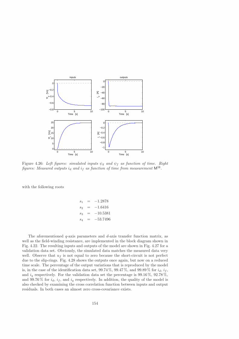
0 5 10−100

−80

−60

−40

−20

0

Time [s]

i d [A

]

outputs

0 5 10−0.8

−0.6

−0.4

−0.2

0

Time [s]

Ψd

[Vs]

inputs

0 5 10

−1

−0.8

−0.6

−0.4

−0.2

0

Time [s]

i f [A

]

0 5 100

5

10

15

20

25

Time [s]

Ψf

[Vs]

Figure 4.26: Left figures: simulated inputs ψd and ψf as function of time. Rightfigures: Measured outputs id and if as function of time from measurement M18.

with the following roots

s1 = −1.2878s2 = −1.6416s3 = −10.5381s4 = −53.7496

The aforementioned q-axis parameters and d-axis transfer function matrix, aswell as the field-winding resistance, are implemented in the block diagram shown inFig. 4.22. The resulting inputs and outputs of the model are shown in Fig. 4.27 for avalidation data set. Obviously, the simulated data matches the measured data verywell. Observe that uf is not equal to zero because the short-circuit is not perfectdue to the slip-rings. Fig. 4.28 shows the outputs once again, but now on a reducedtime scale. The percentage of the output variations that is reproduced by the modelis, in the case of the identification data set, 99.74%, 99.47%, and 99.89% for id, if ,and iq respectively. For the validation data set the percentage is 99.16%, 92.78%,and 99.76% for id, if , and iq respectively. In addition, the quality of the model isalso checked by examining the cross correlation function between inputs and outputresiduals. In both cases an almost zero cross-covariance exists.

154

0 5 10

0

5

10

ud

[V]

inputs

0 1 2 3

0

5

10

Time [s]

uq

[V]

0 5 10−1.5

−1

−0.5

0

0.5

uf

[V]

0 5 10−100

−50

0

i d [A

]

outputs

0 1 2 3−100

−50

0

Time [s]

i q [A

]

0 5 10

−1

−0.5

0

i f [A

]

Figure 4.27: Left figures: measured inputs ud, uf and uq as function of time. Rightfigures: outputs id, if and iq as function of time. Solid lines: measured data (vali-dation data set), and dashed-lines: simulated data.

−0.1 0 0.1 0.2 0.3 0.4 0.5−100

−50

0

i d [A

]

outputs

−0.1 0 0.1 0.2 0.3 0.4 0.5−100

−50

0

Time [s]

i q [A

]

−0.1 0 0.1 0.2 0.3 0.4 0.5

−1

−0.5

0

i f [A

]

Figure 4.28: Outputs id, if and iq as function of time (zoom of right figures inFig. 4.27). Solid lines: measured data (validation data set), and dashed-lines: sim-ulated data.

155

4.4 Conclusions

In this chapter the first verification as well as experimental validation results ofDAWIDUM’s wind turbine module library have been presented. The validation hasbeen subdivided into three distinct parts, viz. mechanical module, electrical module,and complete wind turbine model in order to meet the accuracy demanded by theintended model use. It should be stressed that only the first two validation partsare treated in this thesis. The interested reader is referred to Van Baars [6] fora detailed and systematic treatment of the validation of a complete wind turbinemodel through open field identification experiments.

In the first place the verification and validation of DAWIDUM’s automated sys-tematic structural modeling procedure has been examined by considering six cases.In the first case the procedure has been verified by comparing the exact rotating aswell as non-rotating solutions to the frequency equation for transverse vibration ofan Euler-Bernouilli beam to the ones from the superelement approximation. In thesecond till the fifth case measured non-rotating eigenfrequencies of different rotorblades have been compared to those of the superelement approximation. Finally, inthe sixth case, natural frequencies, mode shapes and time-domain responses acquiredfrom a modal test applied to the Lagerwey LW-50/750 wind turbine and the onesfrom a DAWIDUM wind turbine model are compared. The following conclusions canbe drawn:

• DAWIDUM’s automated systematic structural modeling procedure approxi-mates the dynamics effectively as a collection of rigid and flexible bodies;

• The resulting models are suited for both model based control design and designoptimization purposes since the first bending modes are approximated withonly a few superelements;

• The model accuracy is strongly limited by the quality of the supplied inputdata. This implies that, depending on the intended model use and quality ofthe supplied data, tuning of the torsional spring constants using experimentalmodal test data might be required to reach the required model accuracy.

Secondly, the validity of DAWIDUM’s procedure for identifying the transfer func-tions of Park’s dq-axis model describing the electromagnetic part of a synchronousgenerator has been examined by comparing time-domain simulations with measure-ments taken from the Lagerwey LW-50/750 generator. The required input-outputdata is obtained from the modified step-response test. The following conclusions canbe drawn:

• The parameters of Park’s dq-axis model describing the electromagnetic part ofa synchronous generator can be easily and accurately identified following thedeveloped procedure on the basis of modified step-response data;

• It is justified to use this model for model based control design purposes. Theultimate validation of the method and its impact on variable speed wind tur-bine performance can be proved only after the implementation of the designedfrequency converter controller in the Lagerwey LW-50/750 wind turbine.

156

In Chapter 6 the validated model will be used to develop a new, but preliminaryrectifier frequency converter controller to achieve the required high dynamic perfor-mance of the Lagerwey LW-50/750 wind turbine direct-drive synchronous generator.

157

158

Chapter 5

Model parameter updatingusing time-domain data

Assessing design changes in wind turbines from simulation results requires both ac-curate dynamic models and accurate values for the (physical) model parameters.For various reasons, however, the theoretical predictions do often not fully corre-spond with the experimental measurements. Consequently, the model parametersneed to be tuned or updated so as to achieve better correlation with the test data.This should be done in a physically meaningful way, because only in that way it ispossible to give direct feedback to the wind turbine designers.

This chapter addresses the subject of updating the physical parameters of thestructural models derived in Section 3.4 using input-output data acquired from ex-perimental tests. Section 5.1 gives a short introduction to model parameter updatingand its relation to system identification. The problem of parameter identifiabilityis treated in Section 5.2. The developed model parameter optimization procedureis presented in Section 5.3. In Section 5.4 this procedure is verified using simulateddata.

5.1 Introduction

Model parameter updating or model parameter tuning can be defined as a model-based methodology for the reconciliation of measured and simulated data. In otherwords, the goal of model parameter updating is to improve the accuracy of mathe-matical models by adjusting the tunable parameters so that the differences betweensimulated and measured dynamic properties vanish. A question that can be askedis: “What is the relationship between model parameter updating and system iden-tification?”

Recall that system identification deals with constructing mathematical modelsof dynamical systems from experimental data. Basically, there are three types ofidentification, viz. black-box, grey-box, and white-box identification. Black-box

159

identification deals with the situation where a model is identified purely on thebasis of measured data and a given “universal” model class. The models within thisclass can be either linear, such as the common ARX (Autoregressive with externalinput) structure, or non-linear, such as Hammerstein models or neural networks[17]. As a consequence of the model being identified purely on the basis of measureddata rather than reflecting the physical structure, the parameters and states in ablack-box model might not have any physical interpretation. Grey-box identificationcorresponds to the case where physical laws are applied to arrive at the model, butwhere (some of) the physical parameters are unknown (or are not exactly known) andshould be estimated (or updated) from measured input and output data. In grey-box identification both prior information and experimental data are used. Becauseof the fact that the estimated parameters have physical meanings it is possible tocompare the estimated values with information from other sources, such as likelyranges and values in the literature. Furthermore, a model reflecting the physicalstructure will produce models with a wider validity range than black-box models.As a consequence, a grey-box model may require fewer parameters to be updated toachieve the same quality as its black-box counterpart. White-box identification, onthe other hand, deals with pure physical modeling (i.e. first principles modeling).That is, the modeling is performed without the use of experimental data. Whiteand black-box identification can thus be viewed as extreme cases.

In essence, model parameter updating is thus not different from grey-box identi-fication. The term “grey-box identification” is common in control system analysis,while the term “model parameter updating” is used in the field of structural dynam-ics. Similar to black-box identification, model parameter updating requires selectionof the input-output data, a criterion (or objective function), and a model class. Inthis thesis the model class is defined by the physical model structure presented inSection 3.4. It is thus assumed that structural dynamics of a flexible wind turbinecan be approximated adequately by a superelement model. Consequently, the modelstructure is known a priori.

The main two advantages of model parameter updating are that the model struc-ture reflects that of the physical system and that the tunable parameters have a clearphysical interpretation since they are directly related to the geometry and materialproperties. The former advantage allows the calculation of an initial parameter esti-mate that is close to the real parameters. The latter advantage offers the possibilityto establish a bilateral coupling between the design of a new wind turbine and thedesign of its control system. The main disadvantage is that the objective functionis generally a non-linear (and non-quadratic) function in the (user-selected) tun-able parameters. Consequently, no analytic solution exists and minimization of theobjective function can only be obtained through methods of iterative search (i.e. nu-merical optimization). After all, trial and error becomes impractical for more thanthree or four parameters. Such a minimization can cause difficulty and/or failure tocalculate the desired optimal solution [54]. In addition to this it should be mentionedthat the computational cost of numerical optimization is very high. Fortunately, incase of updating the physical parameters of a structural wind turbine model, theoptimization has to be done only once. However, before the model parameter up-

160

dating can take place, we have to examine whether the tunable parameters can beuniquely (globally or locally) identified from measured input-output data.

5.2 Identifiability of model parameters

This section considers the identifiability of dynamical systems from input-outputdata. Identifiability is concerned with the question whether or not the tunable pa-rameters of a certain model can be uniquely (globally or locally) identified frominput-output observations of the system. In other words: are the identified param-eters unique or does there exist more than one distinct solution that satisfy themeasured input-output data. Obviously, this is an important question that has tobe answered before the model parameter updating can take place (to stress that theanalysis can and should be done before an experiment is carried out, the term apriori identifiability is often used in literature). In addition, the terms “structuralidentifiability” and “deterministic identifiability” also have been proposed.

The first question is whether we can in principle, given perfect (i.e. noise-free)input-output data, extract the correct parameter values. There are three possibleoutcomes, viz. the system is:

• Globally identifiable. A system is globally identifiable if and only if itsparameters can be uniquely determined from measured input-output data forall possible initial estimates of the parameter vector;

• Locally identifiable. A system is locally identifiable when its parameterscan only be uniquely determined from measured input-output data when theinitial parameter estimate is constrained to a small enough neighbourhood ofthe real parameter vector θ0;

• Unidentifiable. A system is unidentifiable if at least one of its parameters inthe parameter vector cannot be estimated uniquely from the measured input-output data. That is, there are a finite (but more than one) number of solutions(i.e. different parameter values) that give identical responses to the sameinput(s). Thus the values found for the tunable parameters after applying anyparameter updating procedure are highly questionable, if not meaningless.After all, the demand that a bidirectional communication between the windturbine design and the controller design has to be established requires that thetunable physical parameters must be uniquely (globally or locally) identifiablein order to be able to quantify them.

Obviously, the outcome is dependent on both the order of excitation of the inputsignal and the model parametrization. Both aspects will be discussed in detail inthe next two subsections.

The identifiability question in the presence of real (i.e. noise contaminated) datais in literature referred to as numerically identifiability, or a posteriori identifiabil-ity. Numerically unidentifiable implies thus that the parameters, although uniquely(globally or locally) identifiable, can not be extracted from the data due to limitedparameter estimation accuracy [86].

161

5.2.1 Persistence of excitation

It is straightforward to understand that the character of the input signal that isapplied during an experiment highly determines the amount of relevant informationthat is present in the data. For example, applying a constant input signal u(t) = c,t ∈ [0, · · · , tf ] (c a constant, and tf the final time) to the system will not result in anoutput signal that contains any information on the dynamics of the system. Observethat in this case only static behavior can be uniquely determined. Consequently, inorder to extract sufficient information from measured data concerning the dynamics,conditions have to be imposed on the character of the input signal.

In order to characterize the so-called “order of excitation”, a distinction have tobe made between quasi-stationary signals (e.g. white noise) and transient signals(e.g. step or pulse) as will be shown below.

Definition 5.1 (Persistence of excitation of quasi-stationary signals) Con-sider a quasi-stationary signal u(t), and let the n × n matrix Rn be defined as thesymmetric Toeplitz matrix

Rn =

Ru(0) Ru(1) · · · Ru(n− 1)Ru(1) Ru(0) · · · Ru(n− 2)

.... . . . . .

...Ru(n− 1) · · · Ru(1) Ru(0)

(5.1)

with Ru(i) ≡ Eu(t)u(t− i), then u(t) is persistently exciting of order n if and onlyif Rn is nonsingular.

Note that a sequence of zero mean, independent random variables (i.e. white noise) ispersistently exciting of any finite order, since for these signals Rn = In for all 1 ≤ n ∈IN. Conversely, when applying the above definition to transient signals, it appearsthat these signals are persistently exciting of order 0. This is inconsistent withthe fact that the dynamics of a linear, time invariant (LTI) system are completelycharacterized with their pulse or step response (modulo initial conditions). Thisimplies that Definition 5.1 is not suitable for application of transient signals.

It is a general rule of thumb that, to identify a model of n independent param-eters, the system has to be excited with an input that is persistently exciting oforder n. The simplest way to achieve this is by ensuring that the input signal is asum of n/2 distinct frequency sinusoids. After all, a sinusoid in principle exhibitstwo degrees of freedom: an amplitude an a phase. This implies that by exciting adynamic system with one sinusoid we can identify precisely two parameters (i.e. asinusoid is persistently exciting of order 2).

In the sequel it is assumed that the experiment has been designed such thatthe measured input-output data is “informative enough”. Meaning that the datacan distinguish between nonequal models. The next question is whether differentvalues of the parameter vector can give equal models. This problem concerns theinvertibility of the model structure (i.e. model parametrization).

162

5.2.2 Model parametrization

The way in which the parameters enter into the model is determined by the para-metrization. Formally, a parametrization Π is a surjective mapping that maps theparameter vector θ onto a specific model M(θ) of a model class M as follows:

Π : θ →M(θ) θ ∈ Θ M ∈ MClearly, different values of θ produce different models. There are many differentways of parametrizing sets of models as meant above. For example, in black-boxsystem identification the most common model set is described in terms of fractions ofpolynomials (e.g. ARX). An important property that a parametrization may exhibitis identifiability. A formal definition of identifiability is adopted from Ljung [166]and is listed below.

Definition 5.2 (Global identifiability) The parametrization Π is locally identi-fiable at θ if

Π(θ) = Π(θ) ⇒ θ = θ ∀ θ ∈ Θ (5.2)

Subsequently, the parametrization Π is globally identifiable if it is locally identifiableat almost all θ ∈ Θ.

Thus a model parametrization is globally identifiable if the mapping Π is injective(and therefore bijective). Therefore, identifiability of a parametrization can be con-sidered as a property of finding a unique value of a parameter vector θ when applyingan identification procedure to find an estimate θ. That is, when a parametrization isglobally identifiable the solution set contains only one element: the real parametervector θ0. However, it is practically impossible (except in a view particular cases)to prove mathematically that the mapping Π is injective [46]. Thus Definition 5.2 ismore a theoretical than a practical tool of investigating identifiability. Consequently,global identifiability is difficult to deal with in general terms [167, 256]. In the nexttwo paragraphs, we shall only briefly discuss identifiability of black-box and grey-boxmodel structures.

Black-box model structures

For single-input, single-output (SISO) systems, the general linear, time invariant(LTI), black-box model structure is given by

A(q)y(t) = q−nkB(q)F (q)

u(t) +C(q)D(q)

e(t) (5.3)

where u(t) the input signal, y(t) the output signal, e(t) a white noise signal, A, B,C, D, and F are polynomials in the delay operator q−1

A(q) = 1 + a1q−1 + · · · + ana

q−na

B(q) = b0 + b1q−1 + · · · + bnb

q−nb

C(q) = 1 + c1q−1 + · · · + cnc

q−nc

D(q) = 1 + d1q−1 + · · · + dnd

q−nd

F (q) = 1 + f1q−1 + · · · + fnf

q−nf

163

The numbers na, nb, nc, nd, and nf are the orders of the respective polynomials.The number nk is the pure time delay (the dead-time) from input to output. Noticethat for a sampled data system, nk is equal to 1 if there is no dead-time. Thevariance of the white noise is assumed to be λ. The coefficients of the polynomialsare collected in the parameter vector θ

θ =[f1 f2 · · · fnf

d1 · · · a1 · · · ana

]T (5.4)

It has been shown in Ljung [166] that the above mentioned black-box modelstructure is globally identifiable provided that the polynomials do not all have acommon factor (i.e. the model can not be represented using a smaller order of thepolynomials).

Grey-box model structures

For grey-box model structures or model structures with physical parameters the sit-uation is much more complex. Except for special structures, there are no generaltechniques available to test for unique identifiability [166]. Intuitively, one would ex-pect a relationship between controllability/observability on the one hand and iden-tifiability on the other hand. Unfortunately, in Walter [303] it has been shown thatcontrollability and observability are neither necessary nor sufficient conditions forthe model to be uniquely (globally or locally) identifiable. Consequently, checkingthe observability and controllability of a given structure does not able us to concludewhether or not the tunable parameters of this structure are identifiable. Note thatlocal identifiability is a necessary conditon for global identifiability.

We limit ourselves to the model class defined by the lumped-parameter modeldescribing the structural dynamics of a flexible wind turbine. This model class hasbeen presented in Section 3.4 and is here referred to as: Mwt

m . That is, we have toexamine whether the tunable parameters in Mwt

m are uniquely (globally or locally)identifiable from measured input-output data. We use the following definition

Definition 5.3 (Global identifiability of Mwtm ) The model class Mwt

m is globallyidentifiable at θ if

ymeas(t, θ) ≡ ysim(t, θ) implies θ = θ ∀ t ∈ IR+ (5.5)

where ymeas the actually measured output and ysim the model output as a functionof the parameter vector θ and time t for a fixed initial condition. The model classis locally identifiable at θ when Eq. (5.5) results when θ is confined to a smallneighbourhood of θ. Note that the size of the neighbourhood of θ is, in general, noteasily found.

Most techniques used to test identifiability, however, rely on the availability ofan analytic expression for the observed outputs as function of the tunable parame-ters. In Appendix G it has been shown that for the model class Mwt

m it is difficultand cumbersome to obtain such an expression. Consequently, we have decided tocheck the identifiability of the model class Mwt

m through simulation. Before theidentifiability can be checked, however, a parameter optimization procedure has tobe developed. This is the subject of the next section.

164

5.3 Off-line parameter optimization procedure

In this section the developed off-line, model parameter optimization procedure ispresented. In Section 5.1 it has been explained that model parameter updating im-plies numerical optimization. In general, optimization concerns the minimization (ormaximization) of a user-specified objective function of several parameters, possiblysubject to restrictions on the values of the parameters defined by a set of constraints(e.g. lower and/or upper bounds on the parameters). In literature it has been shownthat most optimization problems benefit from good initial guesses for the values ofthe model parameters [7]. This improves the execution efficiency and can help lo-cate the global minimum instead of a local minimum. For this reason, the modelparameters of the first principles models of Section 3.4 are used as a starting point.

Solution of optimization problems by a single, all-purpose, method is cumber-some and inefficient. Optimization problems are therefore classified into particularcategories, where each category is defined by the properties of the objective andconstraint functions. Typical objective functions to be minimized are the sum ofsquares and weighted sum of squares. Constraint functions often arise from priorinformation concerning the parameter values. The presence of constraint functions,particularly in the form of upper and lower bounds on each parameter, often exertsa beneficial influence on the convergence of an optimization algorithm [7]. More andWright [194] presented an overview of algorithms for different classes of optimiza-tion problems as well as information on some of the most widely used optimizationsoftware. In this section, the possibilities and limitations of both unconstrained andconstrained optimization will be discussed briefly in order to be able to select themost suitable method for updating the physical parameters of a structural windturbine model.

5.3.1 Unconstrained optimization

The unconstrained optimization problem is central to the development of optimiza-tion software since constrained optimization algorithms are often extensions of un-constrained algorithms, while the non-linear least-squares algorithm tend to be aspecialization. In many algorithms, the objective function is modified in constrainedalgorithms in such a way that it increases drastically as (one of) the parameter valuesapproaches a constraint. To accomplish this, penalty functions are assigned to eachof the constraints. Although many methods exists for unconstrained optimization,they can be categorized into two general classes: direct and indirect search methods.

Direct search methods were the earliest methods used for unconstrained opti-mization and use only function evaluations in determining the search direction. In-direct search methods, on the other hand, require the use of (numerical or analytic)gradient information [54]. The indirect search methods (or “gradient-based searchmethods”) are generally more efficient when the function to be minimized is contin-uous in its first derivative. Direct search methods, which are often also referred toas “function comparison methods”, are claimed to be more robust for problems thatare very non-linear, have a number of discontinuities or where the function valuesare noisy [181]. In contrast, Gill et al. [79] state that “a method using function

165

comparison should be used only when there is no other suitable alternative methodavailable” (e.g. non-smooth objective functions). This statement is confirmed byBard [7]. Direct methods are, however, popular in practice, since they require theuser to supply only function values, not information about the slope of the objectivefunction. However, if a user decides to use a direct method only because of its sim-plicity, a severe price may be paid in speed and reliability (i.e. only a few guaranteescan be made concerning convergence) [79].

Indirect methods

The class of indirect optimization methods is dominated by three basic approaches,viz. Modified Newton methods, Quasi-Newton methods, and Conjugate-Gradientmethods. The distinctions among the three methods arise primarily from the needto use varying levels of information about the derivatives of the objective functionin defining the search direction.

The Modified Newton methods use the Hessian matrix (i.e. matrix of secondpartial derivatives with respect to the tunable parameters), or a finite difference ap-proximation of it (in order to avoid analytic differentiation of the objective function)to compute search directions. Quasi-Newton or variable metric methods approxi-mate the Hessian by a matrix which is built up from iteration to iteration (e.g. fminuuses either the Broyden-Fletcher-Goldfarb-Shanno (BFGS) or the Davidon-Fletcher-Powell (DFP) update formula). This method can be used when the Hessian matrixis difficult or time-consuming to evaluate [194]. Conjugate-Gradient algorithms areideally suited for large-scale optimization, since they do not require the storage of alarge matrix in generating the direction of search. The interested reader is referredto Gill et al. [79] for a full description of the aforementioned methods.

The problem of minimizing a user-specified objective function of several param-eters using gradient information can be stated mathematically as follows

minθFobj(θ)

where Fobj is the objective function and the θ the physical parameter vector (θ ∈ IRn,that is θ = (θ1, θ2, · · · , θn) with n the number of tunable parameters).

The necessary condition for minimizing the objective function Fobj(θ) is obtainedby setting the derivative of Fobj with respect to the parameters to zero, i.e.

∂Fobj

∂θi= 0 i = 1, 2, · · · , n

or∇Fobj = 0

where

∇Fobj =[∂Fobj

∂θ1,∂Fobj

∂θ2, · · · , ∂Fobj

∂θn

]T

which is known as the gradient vector. The terms associated with second derivativesis given by

H = ∇2Fobj

166

The above equation results in a symmetric matrix called the Hessian matrix of thefunction. Once the derivative of Fobj vanishes at local extrema (θ1, θ2, · · · , θn), forFobj to have a relative minimum, the Hessian matrix evaluated at (θ1, θ2, · · · , θn)must be a positive definite matrix. This condition requires that all eigenvalues ofthe Hessian matrix evaluated at (θ1, θ2, · · · , θn) be positive.

In summary, the unconstrained minimum of a function is found by setting itspartial derivatives (with respect to the tunable parameters) equal to zero and solvingfor the parameter values. Among the sets of parameter values obtained, those atwhich the matrix of second partial derivatives of the cost function is positive definiteare local minima. If there is a single local minimum, it is also the global minimum;otherwise, the cost function must be evaluated at each of the minima to determinewhich one is the global minimum.

Direct methods

The three most widely used direct search methods are the Hooke and Jeeves patternsearch method [110], the Nelder and Mead Simplex method [199], and Powell’sconjugate gradient method [210]. In the sequel we discuss in detail only the mostefficient and accurate one: the Nelder-Mead Simplex method (see Onwubiko [204]for a comparison).

The Nelder-Mead Simplex method is based on the “Sequential Simplex” methodformulated by Spendley, Hext, and Himsworth in 1962 [278]. To understand theNelder-Mead method, we need to briefly consider the sequential simplex method.

A simplex in IRn is a set of n+1 points (x0, x1, · · · , xn) which form a polyhedron.In the case of IR2 a simplex is simply a (equilateral) triangle, while in three dimen-sions it becomes a tetrahedron. At each iteration, to minimize the user-specifiedobjective function, the function values are determined at each of the n+ 1 vertices.After that, the vertex with the highest function value is mirrored (reflected) in thecentroid of the other n vertices as illustrated in Fig. 5.1, with the result that a newsimplex is created. The objective function is then evaluated at the new vertex, andthe process is repeated. Observe that the search direction points away from thevertex having the largest function value.

During the iterations after the first one it might be that the newest vertex still hasthe largest function value in the new simplex, and reflecting this vertex would causeoscillation. To prevent this, the largest function value other than that at the newestvertex is subsequently used to decide which vertex to reflect. As the optimum isapproached, the last vertex will straddle the optimum point or be within a distance ofthe order of its own size from the optimum. In the latter case, the procedure cannotget closer to the optimum without reducing the simplex size. The simplex size isreduced (“contracted”) by replacing the other vertices by new ones half way the lastvertex. When the resulting simplex size is smaller than a prescribed tolerance, theiteration is stopped. Thus the optimum parameter vector is determined to within atolerance influenced by the size of the simplex.

The typical progress of the iteration is illustrated in Fig. 5.2 using a functionof two parameters [64]. Vertices 1,2 and 3 form the initial simplex, and increasing

167

Figure 5.1: Reflection to a new point in the Simplex method. Vertices x0 (withlargest function value), x1, and x2 form the initial simplex. The next point (vertex)is x4.

numbers indicate the new vertices added to each iteration. Note that vertex 7 hasthe largest function value for the simplex (4,6,7) but is not reflected immediatelysince it is the newest vertex in that simplex. When simplex (6,9,10) is reached,the procedure cannot get closer to the optimum without reducing the simplex sizeto (6,11,12). The iteration continues again from this simplex until the simplex issmaller than a prescribed tolerance. The interested reader is referred to Buchananet al. [35] and Walters et al. [304] for detailed information (including applications)about the Simplex search method.

Figure 5.2: Illustration of the iteration progress of the Simplex method in two pa-rameters (n = 2). Vertices (1,2,3) form the initial simplex. Succeeding new verticesare numbered starting with 4 and continuing to 10 at which a cycle starts to repeat.Consequently the simplex is contracted to the new simplex (6,11,12). After that theprocedure is continued.

168

The problem with the method thus far is that the use of regular simplices slowsdown the rate of acceleration of the search. It would be more efficient to allow thesimplex to adapt to the local contours of the objective function [181]. Because ofthis, Nelder and Mead introduced the use of nonregular simplices. However, it isknown that the Nelder-Mead method frequently fails to converge to a local minimum.Furthermore, this method is slow and can be applied only to problems in which nis small [194]. In spite of this, it is enormously popular in practice. The mainreasons are twofold. First, it typically produces significant improvement in the firstfew iterations. Second, the Nelder-Mead method uses a small number of functionevaluations per iteration. The interested reader is referred to Lagarias et al. [148]were convergence properties of this method are discussed.

5.3.2 Constrained optimization

The constrained optimization problem differs from the unconstrained minimizationproblem in that at least one of the variables is subject to a restriction on its value.The general constrained optimization problem can be defined as to minimize a non-linear function subjected to non-linear constraints. This situation is encounteredoften in engineering practice because design problems are typically constrained byseveral factors (e.g. prior information concerning a parameter value limits the do-main within the estimate is to be found). The introduction of constraints, however,may create difficulties with regard to obtaining solutions.

The simplest approach to constrained optimization is to transform a constrainedproblem into a single function by adding the constraints to the objective functionand use one of the aforementioned direct search methods [204]. This approach isconvenient because the direct search methods do not require the determination ofthe derivatives of the objective function or constraints. Consequently, this approachis generally applicable because it can be used for functions whose differentiation isdifficult and even for functions whose derivatives are discontinuous. In spite of theseadvantages, direct search methods are often criticized because they are not rootedin any mathematical basis. Criticism not withstanding, direct search methods areoften more practical because of the previously stated reasons.

The main indirect search methods that have been proposed for solving con-strained optimization problems are reduced-gradient methods, sequential linear andquadratic programming methods, and exact penalty functions [194].

The interested reader is referred to the books of Fletcher [64] and Gill et al. [79]for a detailed treatment of constrained optimization theory.

5.3.3 Selecting a method

Based on an investigation of the main properties of both the unconstrained and con-strained optimization methods, the most suitable method for updating the physicalparameters of a structural wind turbine model must be selected. The first step isto investigate the smoothness of the objective function. After all, most algorithmsexclude all problems for which the objective function is not smooth. This ariseswhen finding best solutions to over-determined systems (m > n, where m number

169

of data points and n number of tunable variables) as in data fitting applications. Ingeneral, non-smooth (i.e. non-differentiable) objective functions are more difficultto minimize than smooth (i.e. at least twice continuously differentiable) objectivefunctions.

The general rule in selecting a method for optimization of smooth objectivefunctions is to make use of as much of derivative information as possible [79]. Inour situation it is impossible to analytically determine the gradient vector of Fobj ,since the function is the result of a simulation. Consequently, either the values ofthe derivatives are to be approximated by a finite difference method or a directmethod must be used. Finite difference methods use the first term of the Taylorseries expansion to compute the gradient vector.

Non-smooth problems are generally solved by direct methods, since indirect opti-mization routines assume that the objective function has continuous first and secondderivatives. However, if the objective function has just a “few” discontinuities in itsfirst derivative, and these discontinuities do not occur in the neighbourhood of thesolution, methods designed for smooth problems are likely to be more efficient [79].

It is decided to use a time-domain model parameter updating technique. Fig. 5.3shows a schematic of the implemented model parameter updating procedure. Mea-sured input (force) and output (accelerations) data of a modal test are used asreference. The optimization performs successive simulations on a DAWIDUM modeland changes the tunable parameters in an attempt to minimize the error betweenthe measured (ymeas) and the simulated (ysim) response (i.e. output error). Thatis, the parameters are determined in such a way that the objective function

Fobj(θ) =T∑

t=0

‖ymeas(t, θ0) − ysim(t, θ)︸ ︷︷ ︸eoe

‖ 2

is minimal. ‖ · ‖ denotes the Euclidian norm and θ the physical parameter vector(θ ∈ IRn with n the number of tunable parameters). Note that for the situationthat the system is present in the model set and assuming noise-free data, the outputerror will be zero for the true parameter values (i.e. Fobj(θ0) = 0).

The procedure uses either the Nelder-Mead simplex method or a combined Gauss-Newton and modified Newton algorithm. Both algorithms require function valuesonly. Both objective functions are defined in a MATLAB R© M-file (ObjFun.m andlsfun1.m respectively). The optimization routine (either fmins [91] or e04fdf [197])is invoked in NMstart.m/LSstart.m. Examples of these files can be found in Mole-naar [191].

In the sequel it is assumed that the mass, inertia and length of the rigid bodieswithin the superelements are estimated fairly accurately at the design stage, but thatcalculation of the stiffness and damping parameters may be difficult. Consequently,the tunable parameters are the torsional spring and damper constants. When theuncertainties in mass, inertia or length can not be neglected, however, SD/FAST R©

offers the possibility of leaving systems parameters unspecified in the System De-scription file (using a “?” instead of a number). In addition, a default numericalvalue can be specified immediately before the question mark. For example, the en-

170

Figure 5.3: Schematic of the time domain model parameter updating procedure, withymeas the measured output, ysim the simulated output and eoe the output error.

try: mass = 500? indicates that the initial mass is equal to 500 kg. but that itsvalue can be changed at run time. Thus mass properties and system geometry canalso be treated as variable.

5.4 Verification using simulated data

In this section the identifiability of the model class Mwtm will be checked using

simulation. Furthermore, the proposed parameter optimization procedure will beverified using simulated data before applying it to real data. The optimizationperforms successive simulations on different models from the DAWIDUM mechanicalmodule library and changes the tunable parameters in an attempt to minimize theerror between “measured” and simulated response.

In this way the most suitable optimization method for updating the physicalparameters of a structural wind turbine model can be selected in a systematic way.Two cases are considered. In the first subsection the one superelement approximationof an Euler-Bernoulli beam is used to generate the “measured” data. In the secondsubsection the mechanical model SDLW1 has been used to generate the “measured”data. This section concludes with a discussion.

5.4.1 Beam1sd

In this subsection the one superelement approximation of an Euler-Bernoulli beamis used to generate the “measured” data. This model is referred to as Beam1sd andis depicted in Fig. 5.4. The Euler-Bernoulli beam considered has length L = 50m, modulus of elasticity E = 21 · 1010 N/m2, area of beam cross-section (circular)A = π m2, mass density ρ = 7850 kg/m3, and area moment of inertia I = 1

4π m4.The beam is built in at the base.

171

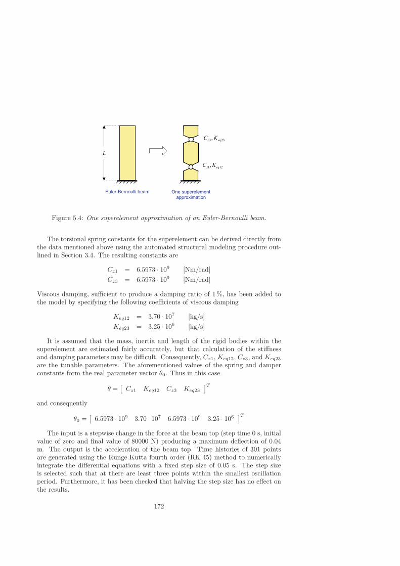
Figure 5.4: One superelement approximation of an Euler-Bernoulli beam.

The torsional spring constants for the superelement can be derived directly fromthe data mentioned above using the automated structural modeling procedure out-lined in Section 3.4. The resulting constants are

Cz1 = 6.5973 · 109 [Nm/rad]Cz3 = 6.5973 · 109 [Nm/rad]

Viscous damping, sufficient to produce a damping ratio of 1 %, has been added tothe model by specifying the following coefficients of viscous damping

Keq12 = 3.70 · 107 [kg/s]Keq23 = 3.25 · 106 [kg/s]

It is assumed that the mass, inertia and length of the rigid bodies within thesuperelement are estimated fairly accurately, but that calculation of the stiffnessand damping parameters may be difficult. Consequently, Cz1, Keq12, Cz3, and Keq23

are the tunable parameters. The aforementioned values of the spring and damperconstants form the real parameter vector θ0. Thus in this case

θ =[Cz1 Keq12 Cz3 Keq23

]Tand consequently

θ0 =[

6.5973 · 109 3.70 · 107 6.5973 · 109 3.25 · 106]T

The input is a stepwise change in the force at the beam top (step time 0 s, initialvalue of zero and final value of 80000 N) producing a maximum deflection of 0.04m. The output is the acceleration of the beam top. Time histories of 301 pointsare generated using the Runge-Kutta fourth order (RK-45) method to numericallyintegrate the differential equations with a fixed step size of 0.05 s. The step sizeis selected such that at there are least three points within the smallest oscillationperiod. Furthermore, it has been checked that halving the step size has no effect onthe results.

172

The objective function is defined as the sum of squares of the difference betweenthe measured and simulated output. The objective is depicted in Fig. 5.5 as afunction of the percentage of variation in the parameter vector θ (i.e. 100% = θ0,and 110% means that the numerical values of all four tunable parameters are set to110% of their real values). Observe the two local minima around 75 % and 125 % ofthe real parameter vector.

25 50 75 100 125 150

0

20

40

60

80

100

120

Variation [%]

Fob

j [m

2/s4

]

Objective function

Figure 5.5: Objective function Fobj of Beam1sd with calculated values.

It is now interesting to determine which parameter variations around the real val-ues of Cz1, Keq12, Cz3, and Keq23 can be allowed such that the estimated parametervector θ still converges to the real parameter vector θ0. That is, determine

max ∆θ0 s.t. θ → θ0

Two noise-free cases and one where a white-noise signal has been added to rep-resent measurement noise are considered in the sequel. The first and third case usethe Nelder-Mead simplex method implemented by the fmins function in the Opti-mization Toolbox of MATLAB R©. The second uses a combined Gauss-Newton andmodified Newton algorithm to minimize the unconstrained sum of squares. The al-gorithm is the so-called e04fdf routine from the Numerical Algorithms Group (NAG)Toolbox [197]. Both algorithms use function values only.

Case 1: Nelder-Mead (noise-free)

Table 5.1 summarizes the obtained results of the noise-free simulations performed onthe DAWIDUM model Beam1sd using the Nelder-Mead simplex method. The first

173

column indicates the run number. The second till the fifth column specify the initialvalues of the tunable parameters. For example, Cz1 = 135% means that the initialvalue of the torsional spring constant between the first and the second rigid body isset to 135% of the real value (i.e. 6.5973 ·109). The sixth column shows the numberof iterations it took to converge to a local or to the global minimum. Notice that inthis simulation example it is possible to make a distinction between a local and theglobal minimum since the real parameter vector is known.

Table 5.1: Model updating results for Beam1sd. Case 1: Nelder-Mead (noise-free).

As expected, the optimization takes many iterations to converge. To illustrate,Fig. 5.6 shows the convergence of the parameters for run NM 6. Observe that thenumber of iterations increases as the initial values of the tunable parameters arefurther away from the real values. Moreover, when the initial values of the tunableparameters differ more than −30% or more than +35% of their real values, themethod fails to converge. Consequently, good a priori parameters are essential forthe error between measured and simulated response to vanish.

Case 2: Least-squares (noise-free)

Table 5.2 summarizes the obtained results of the noise-free simulations performedon the DAWIDUM model Beam1sd using a least-squares method. The first columnindicates the run number. The second till the fifth column specify the initial valuesof the tunable parameters. For example, Cz1 = 135% means that the initial valueof the torsional spring constant between the first and the second rigid body is setto 135% of the real value (i.e. 6.5973 · 109). The sixth column shows the numberof iterations it took to converge to to a local or to the global minimum. Again itis possible to make a distinction between a local and the global minimum since thereal parameter vector is known.

It can be concluded that in this case the least-squares method greatly reducesthe number of iterations. Consequently, the amount of time it takes to performan optimization is decreased, since the majority of the optimization time is spentconducting simulations. Furthermore, the region of convergence is increased from−30% ≤ ∆θ0 ≤ +35% to −40% ≤ ∆θ0 ≤ +45%.

174

0 200 400 6006

7

8

9

10x 10

9

No. iterations

[Nm

/rad

]

Cz1

0 200 400 6004

5

6

7

8

9

10x 10

9

No. iterations

[Nm

/rad

]

Cz3

0 200 400 6002

3

4

5

6

7

8x 10

7

No. iterations

[kg/

s]

Keq12

0 200 400 6000

2

4

6

8

10x 10

6

No. iterations

[kg/

s]

Keq23

Figure 5.6: Convergence of the parameters for run NM 6 (noise-free simulations per-formed on Beam1sd using Nelder-Mead simplex method; initial values of the tunableparameters: Cz1 = Cz3 = 8.9064 ·109, Keq12 = 4.995 ·107, and Keq23 = 4.3875 ·106).

Table 5.2: Model updating results for Beam1sd. Case 2: least-squares (noise-free).

175

Case 3: Nelder-Mead (additive noise)

In practice, the measured input and output signals are contaminated with noise.To make the simulation more realistic, a white-noise signal has been added to the“measured” output to represent measurement noise. The variance of the normallydistributed noise was varied to analyse the effect of the signal-to-noise ratio on theoptimization. Table 5.3 summarizes the obtained results for the various signal-to-noise ratios. The first column indicates the run number. The second column showsthe signal-to-noise ratio. The signal-to-noise ratio is defined as follows:

S/N-ratio = 20 log10

(std(noise-free output)

std(noise)

)[dB]

The third till the sixth column show the deviation of the four parameters from theirreal values after optimization. The deviation is defined as

∆ =real parameter - optimized parameter

real parameter[%]

The seventh column shows the number of iterations it took to converge to a localor to the global minimum. Finally, the eighth column displays the final value of theobjective function Fobj .

Table 5.3: Model updating results for Beam1sd. Case 3: Nelder-Mead (additivenoise).

It can be concluded that noise causes the optimization to converge more slowly(compare run 1 with run 2-6), or even fails to converge to the real values. Especiallythe damping parameters Keq12 and Keq23 are hard to estimate from noise contami-nated data. The deviations from the real values are acceptable up to a signal-to-noiseratio of 30 dB.

The previous three cases have shown the ability of the proposed model param-eter updating procedure to reproduce the known parameter values from simulateddata. This observation gives confidence in its application to data generated by morecomplex models.

As a next step in the verification of the model parameter updating procedure,the mechanical model SDLW1 describing the structural dynamics of the complete

176

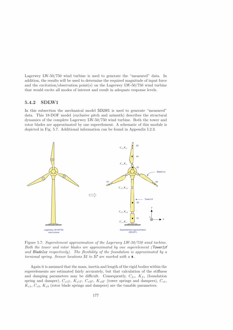
Lagerwey LW-50/750 wind turbine is used to generate the “measured” data. Inaddition, the results will be used to determine the required magnitude of input forceand the excitation/observation point(s) on the Lagerwey LW-50/750 wind turbinethat would excite all modes of interest and result in adequate response levels.

5.4.2 SDLW1

In this subsection the mechanical model SDLW1 is used to generate “measured”data. This 18-DOF model (exclusive pitch and azimuth) describes the structuraldynamics of the complete Lagerwey LW-50/750 wind turbine. Both the tower androtor blades are approximated by one superelement. A schematic of this module isdepicted in Fig. 5.7. Additional information can be found in Appendix I.2.3.

Figure 5.7: Superelement approximation of the Lagerwey LW-50/750 wind turbine.Both the tower and rotor blades are approximated by one superelement (Tower1zfand Blade1xz respectively). The flexibility of the foundation is approximated by atorsional spring. Sensor locations S1 to S7 are marked with a .

Again it is assumed that the mass, inertia and length of the rigid bodies within thesuperelements are estimated fairly accurately, but that calculation of the stiffnessand damping parameters may be difficult. Consequently, Cfz, Kfz (foundationspring and damper), Cz1T , Kz1T , Cz3T , Kz3T (tower springs and dampers), Cz1,Kz1, Cz3, Kz3 (rotor blade springs and dampers) are the tunable parameters.

177

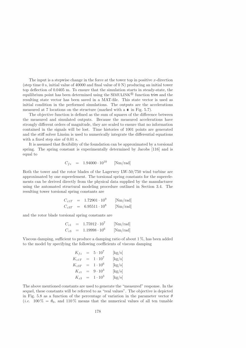
The input is a stepwise change in the force at the tower top in positive x-direction(step time 0 s, initial value of 40000 and final value of 0 N) producing an initial towertop deflection of 0.0405 m. To ensure that the simulation starts in steady-state, theequilibrium point has been determined using the SIMULINK R© function trim and theresulting state vector has been saved in a MAT-file. This state vector is used asinitial condition in the performed simulations. The outputs are the accelerationsmeasured at 7 locations on the structure (marked with a in Fig. 5.7).

The objective function is defined as the sum of squares of the difference betweenthe measured and simulated outputs. Because the measured accelerations havestrongly different orders of magnitude, they are scaled to ensure that no informationcontained in the signals will be lost. Time histories of 1001 points are generatedand the stiff solver Linsim is used to numerically integrate the differential equationswith a fixed step size of 0.01 s.

It is assumed that flexibility of the foundation can be approximated by a torsionalspring. The spring constant is experimentally determined by Jacobs [116] and isequal to

Cfz = 1.94000 · 1010 [Nm/rad]

Both the tower and the rotor blades of the Lagerwey LW-50/750 wind turbine areapproximated by one superelement. The torsional spring constants for the superele-ments can be derived directly from the physical data supplied by the manufacturerusing the automated structural modeling procedure outlined in Section 3.4. Theresulting tower torsional spring constants are

Cz1T = 1.72901 · 109 [Nm/rad]Cz3T = 6.95511 · 108 [Nm/rad]

and the rotor blade torsional spring constants are

Cz1 = 1.75912 · 107 [Nm/rad]Cz3 = 1.19998 · 106 [Nm/rad]

Viscous damping, sufficient to produce a damping ratio of about 1 %, has been addedto the model by specifying the following coefficients of viscous damping

Kfz = 5 · 107 [kg/s]Kz1T = 1 · 107 [kg/s]Kz3T = 1 · 106 [kg/s]Kz1 = 9 · 103 [kg/s]Kz3 = 1 · 103 [kg/s]

The above mentioned constants are used to generate the “measured” response. In thesequel, these constants will be referred to as “real values”. The objective is depictedin Fig. 5.8 as a function of the percentage of variation in the parameter vector θ(i.e. 100% = θ0, and 110% means that the numerical values of all ten tunable

178

parameters are set to 110% of their real values). Obviously, both the Nelder-Meadmethod and the least-squares method should be able to locate the global minimumwithout much difficulty.

25 50 75 100 125 150 175

0

0.2

0.4

0.6

0.8

1

1.2

1.4

1.6

1.8

2

Variation [%]

Fob

j [m

2/s4

]

Objective function

Figure 5.8: Objective function Fobj of SDLW1 with calculated values.

The optimization is started by invoking NMstart.m which sets the initial valuesof the tunable parameters a certain percentage of their real values and subsequentlyperforms successive simulations on SDLW1. The Nelder-Mead algorithm changes thetunable parameters in an attempt to minimize the error between “measured” andsimulated response. In this case, the optimization time can be reduced from 10 to 1second by multiplying the objective function by the time vector t. The explanationis as follows: because t is small in the early stages of the response, it weights earlyerrors less heavily than late errors allowing a reduction of the simulation time.

The numerical results are given in Table 5.4. The first column indicates the runnumber. The second till the sixth column specify the initial values of the tunableparameters. For example, Cz1T = 110% means that the initial value of the torsionalspring constant between the first and the second rigid body of the tower is set to110% of the real value (i.e. 1.72901 · 109). The seventh column shows the numberof iterations it took to converge to a local or to the global minimum. It can beconcluded that the torsional spring and damper constants can be identified uniquelyusing perfect data provided that the initial guess is sufficiently close to the realvalues.

The region of convergence can be increased substantially by first applying theaforementioned least-squares method and subsequently finetuning the results by us-ing the Nelder-Mead direct search method. The results of this case are summarizedin Table 5.5.

179

Table 5.4: Model updating results for SDLW1. Case 1: Nelder-Mead (noise-free)

Table 5.5: Model updating results for SDLW1. Case 2: least-squares and Nelder-Mead (noise-free).

The ability of the presented off-line model parameter updating procedure toreproduce the known parameter values gives confidence for its application to fielddata obtained from a modal test.

5.5 Discussion

The purpose of this section is to briefly revisit the obtained results. In this chapteran off-line, time-domain model parameter updating procedure is presented for theidentification of wind turbine stiffness and damping parameters under the assump-tion that the model structure is known a priori. The procedure tries to produce an

180

updated model which replicates the simulated time-domain data exactly. The pro-cedure uses either the Nelder-Mead simplex method or a combined Gauss-Newtonand modified Newton algorithm. Both algorithms require function values only (i.e.no numerical or analytic gradient information required). This implies that they arewell suited for optimizing objective functions that are noisy or are discontinuous atthe solution.

The parameter optimization procedure has been verified using simulated data.The optimization performs successive simulations on a model from DAWIDUM’smechanical module library and changes the tunable parameters in an attempt tominimize the error between “measured” and simulated response. Two cases wereconsidered: 1) the one superelement approximation of an Euler-Bernoulli beam hasbeen used to generate the “measured” data, and 2) the mechanical model SDLW1has been used to generate the “measured” data. In both cases global optimizationcan be achieved provided that the initial guess is close enough to the real parametervalues. Otherwise, a local minimum will be found.

Having established a validated mathematical model of a flexible wind turbine thatprovides a base for better overall design and control synthesis, we proceed withdeveloping a tool to design a control strategy that reduces the price of the producedelectrical energy.

181

182

Part III:

Model based control design

184

Chapter 6

Frequency convertercontroller design

In the introduction it is stated that to reach economic viability, the design andoperation of the complete wind turbine has to be optimized with respect to bothcost and performance. Reduction of fatigue loads can significantly contribute toachieve this goal. The bandwidth of the active-pitch system, however, is in generaltoo small to be able to achieve fatigue load reduction. As a result, pitch controlshould be used to follow minute-to-minute fluctuations in aerodynamic power, whilethe electromechanical torque control will focus on fatigue load reduction.

Obviously, fatigue load reduction requires almost instantaneous torque controlwhich can only be achieved with a high bandwidth frequency converter controller. Inthis chapter such a controller will be developed for electromechanical torque controlof the direct-drive synchronous generator of the Lagerwey LW-50/750 wind turbine.Section 6.1 motivates the need for an improved frequency converter controller. InSection 6.3 a possible controller configuration is presented after listing the maincontroller objectives in Section 6.2. A new rectifier frequency converter controllerwill be designed on the basis of an identified model of the electromagnetic part of theLagerwey LW-50/750 synchronous generator in Section 6.4. Finally, the conclusionsare presented in Section 6.5.

6.1 Introduction

Modern vector control techniques enable the torque of alternating current (AC) gen-erators to be controlled with a rapid dynamic response. Unfortunately, investigationhas shown that the bandwidth of the frequency converter controller implemented inthe Lagerwey LW-50/750 wind turbine is too small to utilize the potential benefitsof model based control. Consequently, we have decided to develop a new frequencyconverter controller for the direct-drive synchronous generator of the Lagerwey LW-50/750 wind turbine.

185

The frequency converter of the Lagerwey LW-50/750 wind turbine consists of arectifier, DC bus with a smoothing capacitor, and an inverter as illustrated in Fig. 6.1.The frequency converter is located at the tower base. The DC bus capacitor is usedto make the DC input appear as a DC voltage source with a very small internalimpedance at the switching frequency. The rectifier and inverter are connectedback-to-back via the DC bus. The rectifier converts the three-phase alternatingcurrents to 1100 V DC by connecting each of the three stator phases to the positiveor negative side of the DC link voltage. The inverter in turn converts the DC to690 V AC 50 Hz of the utility grid. Because all power is rectified to DC and theninverted to AC the generator is decoupled from the utility grid allowing variablespeed operation.

Both the inverter and rectifier are composed of six power semiconductor devicesor power switches. Each switch consists of an insulated gate bipolar transistor(IGBT) with a reverse diode in antiparallel. The antiparallel diodes provide pathsfor the current independent of the switching state of the IGBT’s.

Figure 6.1: Schematic of back-to-back converter, with SG: synchronous generator,and Si: switch i.

The frequency converter controller in Fig. 6.1 actually consists of two controllers,viz. a rectifier controller and an inverter controller. The rectifier controller forces theelectromechanical torque to equal the torque set-point specified by the wind turbinecontroller. The power quality requirements (e.g. power factor) are controlled bythe inverter (the power factor is often set to unity to obtain zero reactive power).Both goals can be achieved independently of each other by the capacitor decouplingbetween the rectifier and inverter.

6.2 Frequency converter controller objectives

Before we can design a new frequency converter controller we first need to specifythe controller objectives for both the rectifier and inverter controller. The rectifiercontroller objectives can be summarized as:

186

• Controllable electromechanical torque with a closed-loop bandwidth of at least200 Hz;

• Minimize total losses (i.e. stator copper losses, iron losses, converter losses,rotor copper losses, switching losses, and cable losses);

• Reduce the effect of disturbances (including model uncertainties) on the con-trolled torque output of the system.

The main inverter controller objective is to match to grid operator requirements(including power quality issues as: controllable power factor (active/reactive power)and low harmonic disturbances). In the next section a possible controller configura-tion is presented.

6.3 Frequency converter controller configuration

The input to both the rectifier and inverter will be assumed to be a DC voltagesource, as was already assumed in Section 6.1. Such rectifiers and inverters are inliterature referred to as voltage-source converters (VSC). The VSC makes it possibleto connect each of the three generator phases to the positive or negative side of theDC link voltage Udc. Although the shown VSC consists of six IGBT’s with 2 6 = 64different switching states, it is important to realize that the VSC must be operatedso that none of its phases is short-circuiting the link voltage Udc [159]. Hence onlyone of the two switches in each phase can be conductive (e.g. when S1 is turned on,S4 must be turned off).

Figure 6.2: Schematic of a VSC consisting of six IGBT’s and its 2-way switch rep-resentation with the appropriate switch positions.

It is common practice to represent each stator phase as an ideal 2-way switchas shown in Fig. 6.2. This implies that there are 2 3 = 8 different switching states

187

possible. Six of these states yield active vectors (i.e. [Sa Sb Sc] = [1 0 0], [1 1 0],[0 1 0], [0 1 1], [0 0 1], and [1 0 1]) for the terminal stator voltages, and two statesyield zero vectors (i.e. [1 1 1], and [0 0 0]). In the latter two cases the generator isshort-circuited because each of the three-phases is connected to either the positive([Sa Sb Sc] = [1 1 1]) or negative ([Sa Sb Sc] = [0 0 0]) side of the DC link.

The required switching states can be determined in various ways using either themeasured three-phase stator currents or the measured three-phase stator voltages.When the current is used to determine the state of the switches, the VSC is referredto as a current-controlled VSC, otherwise as a voltage controlled VSC. The current-controlled VSC, however, is preferred to the voltage-controlled VSC [26]. The mainreason for the selection of the current as the controlled variable is the same as forthe DC machine: the stator dynamics (stator resistance, stator inductance, andinduced stator voltages or EMF) are eliminated. Consequently, the complexity ofthe controller can be significantly reduced.

There are two ways of implementing current controllers: as AC or as DC currentcontrollers. From a control perspective, DC current controllers are preferred sincethe steady-state currents represented in the rotating dq reference frame are DC

currents [19]. This implies that any current controller with integral action (e.g. aPI-controller) will result in zero steady-state error.

Current controllers for AC machines are, however, more complex than for DC

machines because an AC current controller must control both the amplitude andphase of the three-phase stator currents.

6.3.1 Rectifier controller

A possible rectifier controller configuration that meets the objectives listed in theprevious section is shown in Fig. 6.3. Three main parts can be distinguished:

• Part 1: Frequency converter controller

• Part 2: Voltage-source converter (VSC)

• Part 3: Synchronous generator

The synchronous generator is controlled along the dq model in rotor coordinateswhich corresponds to DC for steady-state. The reference dq currents are transformedinto stator coordinates using Park’s transformation to be then realized by the vectormodulator in the VSC (in rectifier mode). It is assumed that both torque andmechanical speed set-points are calculated by the wind turbine controller such thatthe cost price of electricity generated by the wind turbine is minimal. It should bestressed that all variables used for the control of the synchronous generator are lower-bounded and/or upper-bounded by physical constraints. For example, the currentsare limited to the maximum value that the power electronic components can holdto avoid overheating, and the mechanical speed ωm is limited by the mechanicalconstraints. The aforementioned parts will be treated in detail in the next threesubsubsections.

188

Vecto

rm

odula

tor

supply

au

bu

cu ai bi ci

Contr

olle

r

Contr

olle

r

Se

tpo

int

co

mp

uta

tio

n

di qi

qu

du

set

di

set

qi

m

set

emT

Fre

qu

en

cy

co

nvert

er

co

ntr

oller

VS

C

fu

Supply

Contr

olle

r

set

fi

fi

Ele

ctr

o-

magnetic

part

emT

Syn

ch

ron

ou

sg

en

era

tor

m

qu

du

di qi

Mechanic

al

part

d,

q a,

b,

c

d,

q a,

b,

c

a,

b,

c

d,

q

a,

b,

c

d,

q

Figure 6.3: Control of direct-drive synchronous generator of the Lagerwey LW-50/750 wind turbine in rotating dq-reference frame, with VSC: voltage source con-verter (in rectifier mode).

189

Part 1: Frequency converter controller

The frequency converter controller calculates the desired three-phase voltages thatmust be delivered by the power converter to the generator terminals. The mechanicalspeed ωm and the torque set-point T set

em specified by the wind turbine controller arethe inputs to the frequency converter controller. Comparison of set-point of theelectromechanical torque and its actual value Tem gives an error which serves asinput to the Set-point computation block. The outputs of this block are the referencevalues of the field current iset

f , the direct-axis stator current isetd , and the quadrature-

axis stator current isetq .

The reference value of the field current and its actual value are compared, andtheir difference serves as input to the field current controller (e.g. a PI controller).The output of the field current controller is used to supply a field winding voltageuf to the rotor terminals of the synchronous generator. Similarly, the direct-axisand quadrature-axis stator current set-points are compared with their actual val-ues and the differences are fed to current controllers. The voltage outputs (in thesynchronously rotating reference frame) of these controllers, on the other hand, arefirst transformed into the stator reference frame by application of the Park trans-formation. The abc/dq block contains the power-invariant Park transformation(Eq. (3.82)), while the dq/abc block contains the its inverse.

In the block diagram of Fig. 6.3, it is assumed that the stator currents ia, ib,and ic are measured. Notice that, when the generator is star connected, only twostator current measurements are necessary to compute both id and iq [220]. Afterall, in that specific case one of the currents is redundant because, due to the isolatedneutral,

ia + ib + ic = 0

is valid at any instant. Furthermore, exact knowledge of the mechanical rotor angleθ is needed to transform the AC quantities in the stator reference frame to DC

quantities in the synchronously rotating reference frame and vice verse. In the sequelof this section it is assumed that θ is measured using a position sensor and that theelectromechanical torque Tem is also available (either measured or estimated usingan observer).

Part 2: Voltage-source converter

The VSC contains a vector modulator. The vector modulator forces the three-phasestator voltages to equal their reference voltages. The rectifier switch control signalsare determined using a prestored table of optimal gate switching. It is assumed thatthe three-phase stator voltages equal the reference values within the elapsed timebetween two switching instants. This assumption is justified if the desired closed-loop bandwidth is small compared to the switching frequency. Provided that thisassumption holds, the vector modulator can be modeled as a dead time of length

Tswitch =1

fswitch

with fswitch the switching frequency.

190

Observe that if the VSC was ideal such that the actual three-phase stator voltageswere instantaneously equal to their reference voltages, the block diagram could besimplified by omitting all Park’s transformation blocks (hereby assuming that θ aswell as the machine model is ideal). However, it is preferred that the physical systemstructure is maintained.

Part 3: Synchronous generator

The mathematical model of a synchronous generator consists of two main parts,viz. an electromagnetic and a mechanical part. The electromagnetic part containsthe voltage and flux equations of the synchronous generator as described in Sec-tion 3.5. This model has been identified, verified and validated in Section 4.3 usingexperimental data. The mechanical part is not a separate model but is contained inthe model describing the structural dynamics of the complete turbines as derived inSection 3.4 and validated in Section 4.2.

6.3.2 Inverter controller

The VSC connected to the grid is set to control the voltage level of the DC linkindependent of the operating point of the generator-rectifier subsystem. The maingoal is to set the reactive power demand to zero to obtain unity power factor. But,if the grid is weak (i.e. has a non-negligible, short-circuit impedance), the reactivepower can be used to control the voltage level of the grid. In the sequel it is assumedthat the grid can be modeled as an infinite bus (i.e. voltage source of constantvoltage and frequency). Furthermore, it is assumed that the inverter control loopis fast enough to maintain the DC link voltage at its reference value. Hence, itsoperation does not affect the wind turbine dynamics.

6.4 Rectifier frequency converter controller design

In this section a new, but preliminary rectifier frequency converter controller willbe designed on the basis of the validated model of the electromagnetic part of theLagerwey LW-50/750 synchronous generator. The adjective “preliminary” is used tostress that we will focus on the first controller objective only. As a consequence, noattention will be paid to minimize the total losses and disturbance rejection (secondand third controller objective).

6.4.1 Open-loop analysis

First an open-loop analysis is performed on the identified, verified and validatedmodel of the Lagerwey LW-50/750 synchronous generator to determine possiblecontrol strategies. Consider the (open-loop) Bode magnitude diagram from inputsud, uf , and uq to outputs id, if , and iq shown in Fig. 6.4 (be aware of the differentscales of the y-axes). The solid lines correspond to the standstill case; the dashedlines to the case in which the synchronous generator is rotating at rated speed (i.e.

191

ωm ≈ 2.82 [rad/s], see Table A.4 on page 226). The Bode magnitude plot is createdby selecting the appropriate inputs and outputs from the identified synchronousgenerator model, and subsequently linearizing it about the aforementioned operatingpoints. As the plots reveal, the synchronous generator dynamics strongly depend onthe mechanical rotational speed ωm. As expected, there is no interaction betweenthe direct-axis and the quadrature-axis at standstill.

Frequency [Hz]

Mag

nitu

de

[abs

]

From: uf

0.01 1 100

From: uq

0.01 1 1000.01 1 1000

5

10

15

20

To:

iq

0

0.05

0.1

0.15

0.2

To:

i f

0

50

100

From: ud

To:

id

Figure 6.4: Open-loop Bode magnitude diagram from inputs ud, uf and uq to outputsid, if and iq. Solid lines: standstill case, and dashed lines: synchronous generatorrotating at rated speed (ωm ≈ 2.82 [rad/s])

6.4.2 Set-point computation and controller design

The design of a robust frequency converter controller is based on two tasks: de-termining the structure of the controller and adjusting the controller’s parametersto achieve an “optimal” controlled synchronous generator behavior. Our main con-troller design objective is that the electromechanical torque should exactly and in-stantaneously reproduce its set-point with a bandwidth of at least 200 Hz. That is,the system’s closed-loop transfer function should be as flat and as close as possibleto unity up to 200 Hz for the identified synchronous generator model and designedcontroller combination. Another important goal is to minimize power losses (i.e.maximum efficiency) and to reduce the effect of disturbances on the output of thesystem. Recall that the stator copper losses, converter losses, and cable losses areproportial to the stator current squared, the rotor copper losses are proportial to thefield current squared, and the iron losses to the square of the voltage (see Eq. (3.112)to Eq. (3.119) on page 101-102).

192

Set-point computation

From Eq. (3.114) and the set of equations Eqs. (3.105) it is evident that we needmore information to select for each value of the reference electromechanical torqueT set

em unique values of isetd , iset

q , and isetf . This additional information may be obtained

through an optimization criterion such as: maximum torque per current, maximumtorque per flux, maximum efficiency etc. In the sequel it is assumed for simplicitythat:

1. The field winding current if is kept constant for achieving maximum torqueper ampere (except when field weakening would be required to meet the ob-jectives);

2. The reference value of the direct-axis current isetd is set to zero. The main

reason is that the time constant of the dominating pole associated with the d-axis is about fifteen times larger than that of the q-axis (compare the numericalvalue of s1 on page 153 with the one on page 154). This implies that iq ispreferred to id as the controlled variable for fast torque response.

This implies that the electromechanical torque is proportional to the quadrature-axiscurrent according to:

Tem(3.114)

= p (ψd · iq − ψq · id︸ ︷︷ ︸=0

) ⇒ isetq =

T setem

pψd

with p the number of pole-pairs, ψd, ψq and id, iq the direct- and quadrature-axisstator flux linkages and currents, respectively. The result being that the torquecan be adjusted as accurately and as rapidly as the quadrature-axis current can beadjusted and controlled.

Controller design

Recall that there are several options to control the torque of AC machines via thecurrents. We have decided to use synchronous frame PI or DC current control since itallows a fixed switching frequency (unlike hysteresis control), and yields zero controlerror at steady-state (unlike stator-frame or AC current control). The controllerblocks in Fig. 6.3 thus contain (parallel) PI controllers. The parallel PI controller isdescribed by the following transfer function

Gpi(s) = P +I

s

=P s+ I

s

=P ( s+ I

P )s

with P the proportional gain, and I the integral constant. Obviously, the zero ofthe above transfer function is given by

z = − I

P

193

Therefore a PI controller introduces a transfer function with one pole at the originand one zero that can be located anywhere in the (left-hand) s-plane. The objectiveis thus to choose the parameters P and I to meet the performance specificationsand have desirable robustness properties. Unfortunately, it is not immediately clearhow to choose the parameters in the PI controllers to obtain certain performanceand robustness characteristics. The controller parameters P and I are determinedby trial and error such that the desired performance is achieved without violatingthe following current and voltage limits:

0 ≤√i 2d + i 2q ≤ 340A

0 ≤√u 2

d + u 2q ≤ 690V

The performance of the resulting closed-loop system is treated in the next subsection.

6.4.3 Closed-loop analysis

The simulated closed-loop response of the electromechanical torque of the LagerweyLW-50/750 synchronous generator to a number of stepwise changes in its referencevalue for ωm = 2.0 rad/s is shown in Fig 6.5. Observe that the response has beennormalized with respect to the nominal electromechanical torque. For convenience,Fig. 6.6 shows a zoom of the response after the second stepwise change. It can beconcluded that electromechanical torque can considered to be instantaneously con-trolled considerably over 200 Hz due to the high bandwidth of the designed currentcontrollers. Consequently, for wind turbine time-domain simulation purposes, it suf-fices to use a first order model of the generator plus frequency converter. The timeconstant can be derived from the torque response time.

It must be noted that when the electromechanical torque set-point T setem changes

(and thus the set-point for iq), a transient error in id results, since the PI currentcontrollers work in two single loops. To combat this, more advanced MIMO currentcontrollers are required.

6.5 Conclusions

In this chapter a preliminary frequency converter controller has been developed forthe validated model of the Lagerwey LW-50/750 synchronous generator. It has beenshown that, under the assumptions made, the generator plus conversion system canbe viewed as an (almost) instantaneous torque source within the specified bandwidthusing single loop PI current controllers. No effort has been put in to either minimizethe power losses or to reduce the effect of disturbances. It is expected that theperformance can be even further improved (or harmonic content can be reduced) bydesigning more advanced controllers (e.g. MIMO current controllers) that exploitthe interaction which exists between the d and q components of the stator voltageand current.

194

0 0.5 1 1.5 2 2.5−0.2

0

0.2

0.4

0.6

0.8

1

Time [sec]

Tem

[−

]

Figure 6.5: Normalized electromechanical torque response of PI-controlled LagerweyLW-50/750 synchronous generator to a number of stepwise changes in the torqueset-point T set

em .

1.5 1.5005 1.501 1.5015 1.502 1.5025 1.503

0.836

0.8368

0.8376

0.8384

0.8392

0.84

0.8408

Time [sec]

Tem

[−

]

Figure 6.6: Zoom around the second stepwise changes.

195

196

Chapter 7

Economic control design

In this chapter the first steps towards the development of a wind turbine controlsystem design methodology with an economic objective function will be made bypresenting some design guidelines. Eventually, we will arrive at a methodology thattranslates the manufacturer’s specifications as well as site-specific data automaticallyin a purpose-made controller. Together with the systematic approach developed inPart I and verified and (partly) validated in Part II, this will lead to an integratedand optimal wind turbine design. Consequently, this may help to close the gap thatexists between the control engineering and the wind engineering community.

In Section 7.2 following the introduction, closed-loop wind turbine control issueswill be discussed. In Section 7.3 a breakdown of cost of generating electricity usingwind turbines as well as ways to reduce the cost will be presented. Finally, inSection 7.4 design guidelines are presented.

7.1 Introduction

The previous chapters have discussed the modeling of the wind input as well as themodeling and coupling of the aerodynamic, mechanical and electrical module of aflexible, variable speed onshore wind turbine. To successfully extract electrical powerfrom the wind, a wind turbine also needs a control system that ties the operationof the aforementioned modules together. In general, a wind turbine control systemhas to carry out following two functions:

• Supervisory control

• Closed-loop control

The supervisory control system manages and monitors the switching between thevarious wind turbine modes of operation (see Appendix E for an overview of themain modes) and performs the reporting to the turbine operator(s). The main goalof the closed-loop control system is to enhance the overall performance aiming atboth cost reduction and performance increase. It must be noted that the supervisory

197

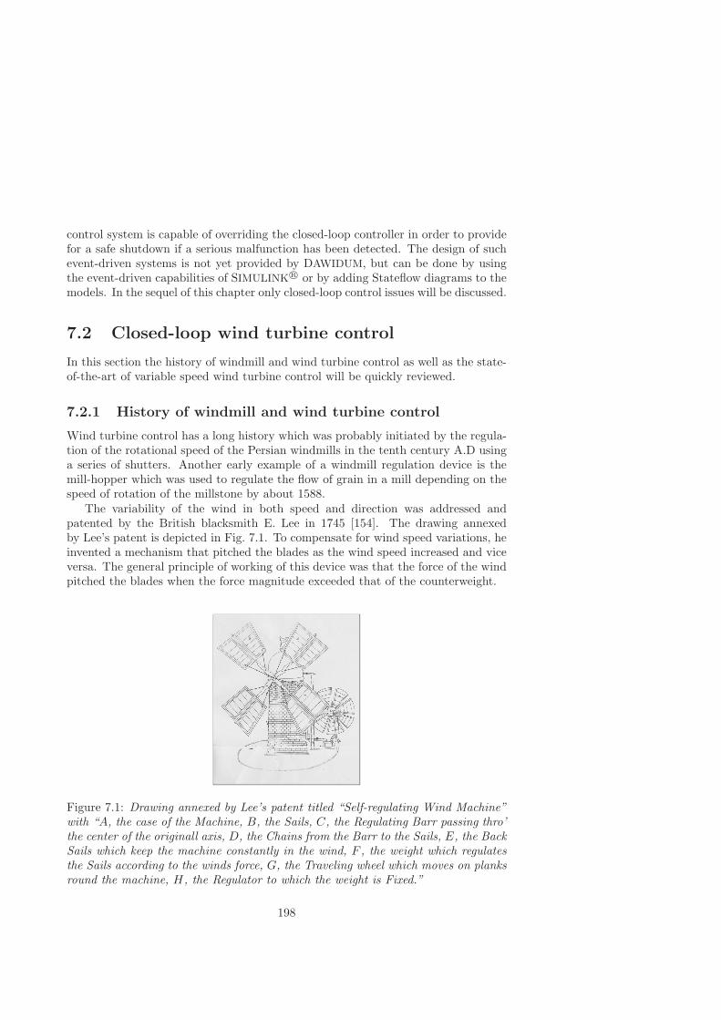
control system is capable of overriding the closed-loop controller in order to providefor a safe shutdown if a serious malfunction has been detected. The design of suchevent-driven systems is not yet provided by DAWIDUM, but can be done by usingthe event-driven capabilities of SIMULINK R© or by adding Stateflow diagrams to themodels. In the sequel of this chapter only closed-loop control issues will be discussed.

7.2 Closed-loop wind turbine control

In this section the history of windmill and wind turbine control as well as the state-of-the-art of variable speed wind turbine control will be quickly reviewed.

7.2.1 History of windmill and wind turbine control

Wind turbine control has a long history which was probably initiated by the regula-tion of the rotational speed of the Persian windmills in the tenth century A.D usinga series of shutters. Another early example of a windmill regulation device is themill-hopper which was used to regulate the flow of grain in a mill depending on thespeed of rotation of the millstone by about 1588.

The variability of the wind in both speed and direction was addressed andpatented by the British blacksmith E. Lee in 1745 [154]. The drawing annexedby Lee’s patent is depicted in Fig. 7.1. To compensate for wind speed variations, heinvented a mechanism that pitched the blades as the wind speed increased and viceversa. The general principle of working of this device was that the force of the windpitched the blades when the force magnitude exceeded that of the counterweight.

Figure 7.1: Drawing annexed by Lee’s patent titled “Self-regulating Wind Machine”with “A, the case of the Machine, B, the Sails, C, the Regulating Barr passing thro’the center of the originall axis, D, the Chains from the Barr to the Sails, E, the BackSails which keep the machine constantly in the wind, F , the weight which regulatesthe Sails according to the winds force, G, the Traveling wheel which moves on planksround the machine, H, the Regulator to which the weight is Fixed.”

198

In addition, for keeping windmills pointed into the wind he developed the fantail:an auxiliary set of blades located behind and oriented perpendicular to the rotor.This yaw mechanism turned the cap of a tower mill automatically into the wind,thereby eliminating the need for manual changes in the windmill’s orientation. Thefantail thus had the ability to follow the changes in wind direction and is one of theearliest applications of feedback control.

Proportional feedback in the form of a centrifugal or fly-ball governor was usedto regulate the speed of grain grinding windmills by controlling the force betweenthe millstones around 1750 [5]. It must be noted that, in 1788, James Watt used asimilar system for speed control of steam engines. The fly-ball governor and linkagekept the millstones apart, allowing the rotor to run unloaded up to a specifiedrotational speed. At this speed, the fly-balls rose up and allowed the millstones tomove together and absorb torque. As the wind ramped up, the miller increased theflow rate of grain to absorb more torque. If the wind increased even more, it wasnecessary to turn the rotor out of the wind and stop it. Next, the sheets of canvasthat were stretched over the wooden framework of the sails were reefed in order toreduce the swept area, and the milling process could be restarted. The spring sail,invented by the Scottish millwright A. Meikle in 1772, replaced the sheets of canvaswith a series of wooden shutters. The openings of the shutters could be adaptedmanually by pulling on a chain or rope attached to a system of levers to “spill” thewind. One difficulty with both methods was that the windmill had to be stopped inorder to adjust the settings in case the strength of the wind altered. This problemwas resolved in 1807 by W. Cubit who introduced the patent sail. In this designall the shutters of all the sails were controlled automatically by a counterweightsuspended outside the windmill.

In the windmill era there was, in principle, thus no need to closely control therotational speed. In fact, allowing the windmills to operate at variable speed washighly advantageous as it increased the total energy extracted from the wind. Thesame holds true for the turbines that harnessed the wind for battery charging at thestart of the electric era. The majority of these turbines were equipped with a DC

generator, had blades with a fixed pitch angle and were operated at variable speed.In the early to mid-1970’s, the need for supplying AC power to the grid changed thedemands on wind turbine control because of the the fixed relationship between thespeed of the AC generators and the fixed utility grid frequency. Consequently, themajority of the machines were operated at constant speed and had pitchable bladesto level off excess power.

The control of the constant speed of commercial turbines has been done pre-dominantly using PI-controllers with additional lead-lag and notch filters, while insimulation studies more advanced control strategies were proposed and explored(including optimal control [93, 179, 205] and gain-scheduled controllers [158]). Themajority of the simulation studies followed a format of applying (advanced) controlsystem design to not yet validated and often over-simplified turbine models, followedby simulation based performance comparisons. These performance comparisons arealmost invariably based on measures of pitch angle, shaft speed and power varia-tions. Fair comparisons between the industry standard control system and more

199

advanced controllers, however, are scarce. Knudsen et al. [138] compared a robustcontroller with the existing PI-type controller of a 400 kW commercial wind tur-bine. The robust controller, designed on the basis of an identified turbine model,achieved a reduction of pitch activity and some potential for fatigue load reductioncompared to the existing controller. The comparison confirmed that improvementin performance can be achieved by proper control. The interested reader is referredto La Salle et al. [245] for a more thorough review of constant speed pitch controlledwind turbines as late as the 1990’s.

The majority of the wind turbines now in operation are three-bladed, stall regu-lated constant speed turbines 1[172]. It must be stressed that in this case the bladepitch angle is fixed and, as a consequence, no control possibilities exist at all. Re-call that stall utilizes the inherent aerodynamic properties of a rotor blade to limitthe aerodynamic power. In the sequel, however, we will focus our attention on theclosed-loop control of grid-connected, variable speed pitch-regulated turbines sincethis configuration has the highest potential to reach cost-effectiveness in the (near)future.

7.2.2 State-of-the-art variable speed wind turbine control

In a variable speed wind turbine, the rotor and the generator are decoupled fromthe grid by the power electronics implying that the rotor may rotate at (almost) anyspeed. Consequently, variable speed operation offers more control possibilities thanconstant rotational speed does. Variable speed operation has two main advantagesover constant speed operation: i) additional energy capture at partial load and ii)potential reduction of fatigue loads on the structure by absorbing torque fluctuationsin the rotor momentum. Other benefits that have been claimed are enhanced util-ity grid system compatibility, controllable power factor, reduction of acoustic noiseat low wind speeds, adaptation to local conditions or compensating for changingconditions, and avoidance of stall over most the operating range [186].

In the context of maximum power extraction in partial load, the effect of variablespeed is easily described. The kinetic energy content of the wind passing throughthe rotor varies with the cube of the wind velocity as illustrated in Fig. 7.2. Onlya fraction of this energy can be extracted by the rotor (and subsequently convertedinto electrical power) as explained in Section 3.3. This fraction is denoted by thepower coefficient Cp, which is a function of the tip-speed ratio λ (i.e. the ratio ofrotor circumferential speed to wind velocity) and the blade pitch angle θ. Usually,the power coefficient has one distinct maximum at the optimal tip-speed ratio andblade pitch angle. Practically achievable maximum values are in the range of 0.40 <Cp < 0.50, while common optimum values of the tip-speed ratio lie between 5 and 10depending on the aerodynamic properties of the wind turbine configuration underinvestigation.

It is thus desirable to let the wind turbine rotational speed vary over a widerange, since maximum energy is extracted if the turbine operates constantly at or

1Most megawatt sized wind turbine models that are installed recently and the ones under de-velopment are, however, of the pitch controlled variable speed type

200

0 5 10 15 20 25 300

1000

2000

3000

4000

5000

6000

7000

8000

Vw [m/s]

Pw

[kW

]

Pw ∝ V

w 3

Figure 7.2: Total power in the wind passing through a 25-meter diameter rotor asfunction of the wind velocity.

near its optimum tip-speed ratio. Observe that variable speed operation is notpossible in case that the generator is directly connected to the utility grid. Toallow the generator rotational speed to vary to extract the maximum amount ofpower, a power electronic interface is thus needed. In such an interface the three-phase generator output is rectified into DC and subsequently interfaced with thethree-phase utility source by means of a power electronic converter as outlined inSection 3.5. In general, a rectifier at the generator side as well as an inverter at theutility grid site is required to provide both control and power quality requirements(including power factor).

The control problem of pitch-regulated, variable speed wind turbines significantlydiffers from that of constant speed wind turbines using pitch regulation. The latterpresents a SISO control problem, while variable speed using pitch regulation presentsa MIMO control problem as the electromechanical torque control loop is added tothe existing pitch control loop. This opens the possibility to exploit the interactionsbetween the inputs and outputs in the system to reduce dynamic loads as well asmaintaining a desired amount of energy production. The current control strategyis to use the fast electromechanical torque control to respond to transients, and aslower pitch control loop to follow minute-to-minute fluctuations in wind speed. Bothloops, however, often carry out their tasks independently by PID-type controllers[30, 283]. Probably, a more cost-effective strategy is couple the two control loopsand make them to interfere constructively. Finally, it must be stressed that in orderto make fair comparisons between the industry standard closed-loop controller andmore advanced ones, it is necessary to i) establish the best possible PID controller,and ii) define criteria by which the performance can be evaluated.

201

The control objectives of the variable speed turbine depend on the operatingregime. Below rated wind speed (or partial load) a common objective is to operatethe turbine at optimum tip-speed ratio until a speed, power or torque limit is reached[245]. Above the rated wind velocity (or full load), power limitation is the maingoal. In literature, various controllers are proposed for the aforementioned operatingregimes. Multivariable controllers are successfully applied in simulation studies bySteinbuch [281] (at full load only, results based on a rather coarse wind turbine modelthat has not been confronted with measured data), Bongers [21] (achieved significantfatigue load reduction of both rotor shaft torque and blade root bending moments inone full load operating condition), and Stol [283] (reduced cyclic blade root bendingmoments by periodic control of the pitch angles). Molenaar [188] examined theeffect of a simple filter controller on the fatigue loads on a model of a 2-bladed 500kW variable speed turbine. It has been shown by comparison of the areas enclosedby the rainflow counts of in total 26 load cases (including power production withor without the occurrence of fault, startups and stops at normal wind conditionsand parking cases as prescribed by the IEC-1400-1 standard [112]) that filtering thegenerator speed before computing a new torque set-point significantly reduces thefatigue loads on blade root (flap direction only), drive-train and tower.

In several other publications (see e.g. [39, 51, 95, 96, 135, 238, 276]) additionalpromising simulation results are shown. Various control design methodologies havebeen applied to models of different variable speed wind turbines in order to meetthe aforementioned control objectives. However, all studies are performed with fairlybasic wind turbine models (either the aerodynamics are approximated by a (static)model stored in a look-up table, or the structural flexibility is neglected). Sensorand actuator dynamics as well as disturbance issues are, in general, not addressed.As a consequence, the obtained results should be handled with care.

At the application side, however, still (too) little convincing results are reportedin literature. Bongers applied robust control to a small experimental test-rig anddemonstrated, in only one operating point, that a robust controller is capable toreduce fatigue loading while simultaneously maintaining a desired amount of energyproduction. De Boer and Mortier [16] presented experimental results of the appli-cation of static optimal output feedback on a 300 kW wind turbine. They showedby comparing time-series that, at full load, the direct current fluctuations can bereduced with almost a factor three with respect to the existing SISO controller. Itis concluded from this that the fatigue loads are reduced as well, although no rain-flow countings or load spectra are shown to illustrate the effect on the fatigue life.Kruger et al. [41, 42, 142] demonstrated the potential of advanced control on anexperimental 33 kW wind turbine. They showed, by comparing load spectra of theblade root bending moments, that i) variable speed operation is capable of reduc-ing mechanical loads when compared to constant speed operation, and ii) advancedcontrol can significantly reduce rotor blade fatigue loads (although at the expenseof a slight reduction in the annual electricity yield).

The quick review of the history and state-of-the-art of (closed-loop) wind turbinecontrol shows that:

• The industry standard closed-loop controller is (still) of the PID-type. It is

202

unkown how the PID controller parameters are determined and to what extentthey are optimized;

• Simulation studies are often performed with fairly basic wind turbine models,while the proposed control strategies are elaborate and, in general, do notaddress the real issue: cost-effective control of the whole operating envelope;

• There is a lack of literature reporting on practical field experience obtainedwith control systems. Many of the applications reported are restricted in thescope to only one operating point;

• For variable speed to become the norm and not the exception in the (near)future, the added cost of power electronics required by most variable-speeddesigns must be clearly offset by the increased electricity yield, reduction infatigue loads and other systems costs, impact on the wind turbine design, andthe added benefit of providing power conditioning for utilities.

As a consequence, significant improvements are still possible to reach the desiredeconomic viability of wind power. The first step is to show on a simulation level thatthe competitive position of wind power can be significantly improved by advancedcontrol. The models used in these studies need to be validated against data acquiredfrom experimental tests. Next, the achieved benefits need to be demonstrated inpractice on a (prototype of a) commercial wind turbine.

The main question is how these controllers can be designed. The controller designmust, in principle, encompass all aspects of both performance and cost, ranging fromenergy production, quality of power, lifetime and safety, through cost-effectiveness,acoustic noise and reliability. Notice that the relative importance of these aspectsmay vary from site to site. For example, a key objective for the design of cost-effectiveoffshore wind turbines will be that the operation and maintenance requirements arereduced to a minimum, possibly at the expense of a somewhat higher wind turbinecapital cost or lower electricity yield. The challenge for the control system designer isthus to specify an economic control design objective that reveals the financial impactof a proper controlled wind turbine. Before we can develop such an objective, wefirst have to determine what makes up the cost of generating electricity using wind.

7.3 The cost of generating electricity using wind

In the introduction it was stated that the capital cost accounts for 70%, and theO&M cost for 6−29% of the cost per kilowatt-hour. The cost of capital include thepurchase price, cost of transporting, assembling, and erecting a wind turbine on site,as well as connecting it to the grid, cost of installing grid lines, and transformers. TheO&M cost, on the other hand, include all troubleshooting, inspections, adjustments,retrofits, preventive as well as unscheduled maintenance performed on wind turbines,and the downtime that accumulates while waiting for parts, instructions, or outsideservices that are not available on site but are required to bring the turbine back inoperation.

203

Thus wind energy is a highly capital-intensive technology, and consequently theeconomics of wind power are highly sensitive to both the size of the capital invest-ment and the interest rate charged on that capital. This in turn means that the costcan be effectively reduced by reducing the capital cost (hereby assuming a given,constant capital interest rate). Besides capital and O&M cost reduction, the com-petitive position of wind power can also be improved by ensuring that the turbineis operating continuously at the best possible performance as well as by minimizingthe difference between the technical and economic lifetime.

Now that we know roughly the breakdown of the cost of generating electricityfrom wind, the question is how can we reduce these cost in order to make it com-petitive with all other electricity sources. From the preceding it can be concludedthat either the cost (both capital and O&M) can be reduced or the performance ofthe turbine can be increased. Both aspects will be discussed in more detail in thenext two subsections.

7.3.1 Performance increase

It is important to realize that the wind turbine performance is achieved to a largeextent during normal operation. The cost, on the other hand, are generated duringall operational modes (including power generation cases with the occurrence of fault,parking at storm, and idling). The energy capture of a variable speed wind turbinedepends for the greater part on its ability to successfully operate at the peak of theCp(λ, θ)-curve in partial load. After all, maximum aerodynamic efficiency is achievedat the optimum tip-speed ratio λ = λopt at which the power coefficient Cp has itsmaximum value: Cp,max. This implies that the electromechanical torque Tem mustbe adapted in proportion to the wind velocity Vw squared (or rotor speed squaredsince Vw = ωrR/λ) to maintain the optimum tip-speed ratio. In steady-state, theelectromechanical torque balances the aerodynamical torque reduced by the amountof any mechanical torque loss in the drive-train. This fact is used in the commonlyused “omega-squared” control law which is given by:

T setem =

ρπR 5Cp,max

2λ 3opt

· ω 2r − Tloss (7.1)

where T setem is the set-point for the electromechanical torque, ρ is the air density, R

is the rotor radius, Cp,max is the power coefficient at the optimum tip-speed ratioλopt, ωr the rotor rotational speed, and Tloss the mechanical torque loss (which mayitself be a function of the rotational speed and torque). Although this relationship isvalid only in steady-state, it is also used dynamically to control the electromechani-cal torque demand of variable speed turbines as a function of the measured rotor (orgenerator speed since, in steady-state, ωg = itr ωr with itr the transmission ratio)speed. The measured rotational speed is often filtered using a first order low passfilter to avoid rapid electromechanical torque set-point changes. This way of con-trolling the electromechanical torque below rated wind speed may work satisfactoryon relatively rigid turbines located on sites with uniform wind fields. More flexible

204

variable speed turbines exposed to more turbulent wind conditions, however, willrequire a dynamic control law taking also the phase information into account.

Fingersh and Carlin [61] applied the “omega-squared” control law to the NRELVariable Speed Test Bed turbine and showed that this resulted in an overall energycapture loss of over 5% when compared with the idealized variable speed opera-tion. Modification of the law indicates a preliminary energy capture improvementof between 0.3% and 3%. It can be concluded that the losses associated with vari-able speed turbines running off the optimal point can be reduced by applying moreadvanced control algorithms to track the optimal tip-speed ratio in partial load.

7.3.2 Cost reduction

From the aforementioned two cost items we need to identify the most important costdriver(s). In the introduction it has been mentioned that fatigue loads on the windturbine structure are the main cause of failure in the present onshore wind turbinedesign. This implies that the current design of the main wind turbine components(i.e. rotor blades, support structure, and drive-train) is driven by fatigue loads. Asa consequence, fatigue loads are an important cost driver. It must be noted thatalready from the very beginning wind turbines have experienced fatigue problems[285]. The early wind turbines were mainly designed using static and quasi-staticanalysis. At best, these rather simple analysis led to over-designed wind turbines,and at worst, to premature field failures. The latter is exemplified by the fact thatalmost all rotor blades have been repaired or replaced in the early California windfarms [284]. Wind turbines installed more recently have demonstrated a substantialimprovement in availability due to the fact that the designers used the gain inwisdom of thousands of hours operating experience. However, with the trend towardsincreasingly lightweight and larger wind turbines operating at variable speed thefatigue problems are not yet solved.

The most fatigue critical wind turbine parts are the rotor blades and their con-nection to the hub [180]. The latter, the so-called blade root, is an area of criticalimportance as it transmits the entire blade load through a relatively small spaceenvelope. The unique combination of steady and fatigue loading on a rotor blademakes this a challenging part of the design. In a design life-time of 20 years a ro-tor blade must withstand at least 10 8 to 10 9 cycles of variable amplitude due togusts, atmospheric turbulence, wind shear, gravity, startup and (emergency) shut-down procedures. Very few data are available in this high cycle fatigue range forthe materials and components used in wind turbines, especially in combination withthe fact that rotor blades are exposed to a hostile environment throughout theirlife-time. Such effects include: temperature fluctuations, rain, thunderstorms, for-mation of ice, hailstones, and erosion from sand particles. Other important parts tobe considered are the rotor shaft torque, rotor thrust, tower foot bending momentand internal stresses at critical points on the structure (e.g. the nodes on a tripodfoundation).

Fatigue loads are characterized by lightly damped structural modes. Addingdamping of the structural modes can significantly reduce the impact of fatigue loads.

205

Both rotor and electromechanical torque control can be used for fatigue load reduc-tion. Active rotor control includes full-span (collective) pitch control (low frequenciesonly), cyclic control, aileron control, and individual blade control [78, 175]. It mustbe stressed that in order to investigate the cost-effectiveness of the aforementionedoptions the availability of a validated model is essential.

7.4 Closed-loop control design methodology: de-sign guidelines

Various design procedures exist for control design and may therefore also be appliedto a wind turbine. They range from “classical” design techniques such as root locusand Bode analysis, via optimal control to techniques based on the minimization ofan objective function through numerical optimization. The proper formulation ofthe objective function in the latter procedure is one of the crucial steps in achievingthe desired closed-loop performance. After all, a poorly formulated criterion willsimply yield a controller that optimally implements the poor design. In general, it isdifficult to translate a verbal statement (e.g. minimum fatigue loads) or a concept ofthe desired objective into mathematical terms. Our controller objective is to arriveat cost-effective design and operation of flexible, variable speed wind turbines. Thatis, we have to minimize the cost per kilowatt-hour. The economic control designobjective should at least include a measure of the (annual) electricity yield, fatigue(representive selection of loads). The exact translation of the performance andcost related to wind turbine construction and operation into an economic modelis, however, beyond the scope of this thesis. We will conclude this chapter withpresenting the five main steps in designing cost-effective wind turbines on the basisof a mathematical model:

• Step 1: Develop a mathematical model using design data from the windturbine manufacturer describing the relevant dynamics of the turbine underinvestigation

• Step 2: Validate the model using experimental data obtained from the turbineunder investigation

• Step 3: Translate the manufacturer’s specifications to an economic objectivefunction that can be solved through numerical optimization

• Step 4: Design a controller on the basis of the validated model by minimizinga specified objective function

• Step 5: Implement the controller and evaluate the closed-loop performance

The aforementioned steps imply the need for a close co-operation between the windturbine designer and the control engineers in order to identify those design param-eters for which the economic objective function is most sensitive.

206

Part IV:

Conclusions andrecommendations

208

Chapter 8

Conclusions

This chapter presents the conclusions of this thesis. In the past decades, the windindustry has grown from a niche business serving the environmental aware intoone that has established itself as the most competitive form of renewable energy.Wind has the potential to play an important role in the future world electricitysupply provided that the cost per kilowatt-hour are further reduced. The cost ofwind-generated electricity can be effectively reduced by steady improvements inboth wind turbine design and operation since wind is a highly capital-intensive andmaintenance-demanding technology.

The challenge of wind energy research lies in developing wind turbines that areoptimized with respect to both cost and performance. A prerequisite for the cost-effective design of such turbines is the availability of a systematic methodology thatgenerates accurate and reliable dynamic models of the complete system within thedesign phase with low modeling effort. The main conclusion of this thesis is thatsuch a methodology has been developed for flexible, variable speed, grid connected,horizontal-axis wind turbines that are equipped with a direct-drive synchronousgenerator and are located on land. The solution to the main thesis problem hasbeen achieved by the successive solution of the following of sub-problems:

• Sub-problem 1.2.1: Modeling of flexible wind turbines

• Sub-problem 1.2.2: Model validation

• Sub-problem 1.2.3: Model based control design

These sub-problems and their respective solutions will be discussed in detail below.We would like to emphasize that the presented solutions must not be regarded asthe one and only ones, although they have proven to be sufficient to solve the mainthesis problem. New demands resulting from, for example, cost developments inboth conventional and renewable electricity sources may call for other solutions inthe (near) future to maintain at least the current share of wind power in the globalelectricity mix.

209

Sub-problem 1.2.1: Modeling of flexible wind turbines

The wind turbine modeling sub-problem has been addressed in Part I (comprisingChapter 2 and Chapter 3). In Chapter 2 an inventory of the state-of-the-art of windturbine design codes has been made. From this inventory it can be concluded thatmost of the design codes have been developed specially to deal with wind turbinedesign calculations and time-domain simulations, but are not suited to solve themain thesis problem. The main reasons are: i) the absence of the indispensablebilateral coupling between the design of a new wind turbine and the design and im-plementation of its control system, ii) model validation has not received the attentionrequired for obtaining economic viability of wind power, and iii) the modeling of theelectromagnetic part of the generator plus conversion system has received too littleattention.

In Chapter 3 the development of a new software tool called DAWIDUM wasdescribed that overcomes the aforementioned shortcomings. It must be stressedthat DAWIDUM continues and combines the work that has already been done in theaforementioned design codes. Within DAWIDUM any wind turbine is modeled as aset of four bilaterally coupled modules (i.e. aerodynamic, mechanical, electrical andcontroller) and one input module (i.e. wind). The main conclusions are groupedper module.

• Wind module. Realistic modeling is essential for wind turbine design andevaluation purposes (since the wind drives the system and at the same timealso acts as the main disturbance). DAWIDUM is coupled to SWING-4 (a 3-Dwind field simulation code) to generate stochastic wind field velocity compo-nents. Alternatively, measured time-varying winds can also be used as input.In addition, some effort is made in modeling the deterministic part of theundisturbed wind velocity.

• Aerodynamic module. The implementation of the rotor aerodynamics inDAWIDUM is based on Glauert’s BEM theory plus the corrections that arecommon to be applied to the quasi-steady momentum theory.

• Mechanical module. Much effort has been put in developing tools thatwould establish a bilateral coupling between the wind turbine design and itscontrol system. The main conclusions are:

– DAWIDUM’s mechanical module is equipped with a systematic procedurefor modeling the structural dynamics of flexible wind turbines. The struc-tural dynamics are modeled as a collection of rigid and flexible bodies.Flexible body dynamics are approximated using superelements. The sys-tematic procedure allows both structural designers and control engineersto rapidly and easily build dynamic wind turbine models. Both the modelconfiguration and complexity can be easily adapted by the user;

– An off-line, time-domain model parameter updating procedure has beendeveloped for updating the (user-selected) tunable parameters of thestructural model when measured (modal test) data is available.

210

• Electrical module. The electrical module contains a dynamic model of theelectromagnetic part of an ideal synchronous generator. This model is obtainedby rewriting Park’s dq-axis model equations such that the model parametersretain their physically meaningful interpretation. In addition, the parametersof the reformulated equations can be easily obtained from measured data.

Sub-problem 1.2.2: Model validation

Model verification and validation issues have been addressed in Part II (comprisingChapter 4 and Chapter 5). In Chapter 4 the verification as well as experimentalvalidation of DAWIDUM’s wind turbine mechanical and electrical module have beengiven, while in Chapter 5 the verification of the parameter updating procedure hasbeen addressed. The main conclusions regarding model validation issues are groupedbelow per module.

• Mechanical module. The main conclusions are:

– The systematic modeling procedure has, after being verified using a testcase, been used to generate the equations of motion of 4 different rotorblades as well as to generate a dynamic structural model of the completeLagerwey LW-50/750 wind turbine. Based on thorough comparison of thesystem’s natural frequencies, mode shapes and time-domain responses itcan be concluded that the superelement models are suited to solve themodeling sub-problem;

– The parameter updating procedure has been verified using simulateddata. It has been made plausible that global optimization is likely tobe achieved provided that the initial parameter guess is close enough tothe real parameter values.

• Electrical module. The validity of DAWIDUM’s procedure for identifying thetransfer functions of Park’s dq-axis model describing the electromagnetic partof a synchronous generator has been examined by comparing time-domain sim-ulations with measurements taken from the Lagerwey LW-50/750 generator.The required input-output data is obtained from the modified step-responsetest. The following conclusions can be drawn:

– The parameters of Park’s dq-axis model describing the electromagneticpart of a synchronous generator can be easily and accurately identifiedfollowing the developed procedure on the basis of modified step-responsedata;

– It is justified to use this model for model based control design purposes.The ultimate validation of the method and its impact on variable speedwind turbine performance can be proved only after the implementation ofthe designed frequency converter controller in the Lagerwey LW-50/750wind turbine.

211

Sub-problem 1.2.3: Model based control design

The wind turbine control design sub-problem has been treated in Part III (compris-ing Chapter 6 and Chapter 7). Two main conclusions are grouped below:

• Electrical module. A preliminary frequency converter controller has beendeveloped for the validated model of the Lagerwey LW-50/750 synchronousgenerator. It has been shown that the PI-controlled generator plus conversionsystem can be viewed as an (almost) instantaneous torque source within thespecified bandwidth;

• Economic control design. The first steps towards the systematic synthesisof model based controllers aiming at cost-effectiveness have been taken. Thepenalty for poor closed-loop control is a less cost-effective wind turbine.

212

Chapter 9

Recommendations for futureresearch

This chapter presents the main recommendations for future research. The recom-mendations originate from the fact that not all ideas gained or questions raisedduring the project term have been explored or answered. The main reason for thisis that priority has been given to first solve the questions that initially seemed themost important ones. The numerous issues that deserve future research are sortedby the three sub-problem as listed in Section 1.2 and will be discussed below.

Sub-problem 1.2.1: Modeling of flexible wind turbines

First of all, given the fact that considerable effort has been put in the developmentof DAWIDUM, a warm recommendation is given to fully exploit the potential ofthis new wind turbine design code. This requires the joint effort of all DUWIND

members to develop and implement new models as well as wind turbine specificanalysis and (control) design tools. In addition, the code must be extended with awave and hydrodynamic module required to compute the water wave forces actingon the support structure of wind turbines located offshore. The latter extension isessential, since the future of wind energy will be in large-scale offshore wind farms.

The gained modeling experience has lead, for most modules, to several recom-mendations for future research. The recommendations are grouped per module.

• Aerodynamic module. The following suggestions can be given to improvethe quality of DAWIDUM’s aerodynamic module:

– An area of great importance and significant uncertainty that deservesattention is that of modeling of skewed wake effects (also referred to asyawed flow, yaw misalignment or oblique flow). From the practical pointof view, yaw misalignment is a fact of life, and is of paramount impor-tance since an important part of fatigue lifetime consumption of rotor

213

blades can be attributed to these conditions. In addition, it is of impor-tance to the load spectra of yaw bearing, tower, and rotor shaft. Hence,corrections must be made to the blade element momentum theory whenthe rotor operates at a yaw angle. Although considerable progress hasbeen made, the results are not yet sufficiently accurate when comparedwith measurements;

– It is recommended to develop an optimization procedure that calculatesthe optimal number of blade elements (independently of the number ofsuperelements) for a given wind turbine configuration.

• Mechanical module. The following suggestions can be given to improve thequality of the models within DAWIDUM’s mechanical module:

– At present, the superelement method used to model the flexible windturbine part considers bending deformation only. It must be noted thatboth axial deflection and torsion (or twist) can be included easily bysubdividing the middle body into two bodies and connecting them usinga joint with one translational and one rotational degree of freedom. Theequations for the computation of the axial and torsional spring stiffnessare given in Molenaar [189]. It is strongly recommended that the torsiondegree of freedom is included when investigating (unknown) aero-elasticinstabilities (e.g. pitch-flap flutter) of especially large rotor blades;

– It is assumed that either the blade designer or the blade manufacturersupplies the mass and the flexural rigidity in the two principal bendingdirection as function of the length of the wind turbines parts that aretreated as flexible. These values are used to compute the required sim-ulation parameters (including the torsional spring constants in bendingdirection). At present, the off-diagonal terms of the rotor blade inertiamatrices (i.e. the products of inertia) and blade twist are neglected. Itis strongly recommended to add this information when available.

• Electrical module. The following suggestions can be given to either improvethe model quality or to increase the model scope:

– In subsection 4.3.3 a MIMO ARX model has been estimated withoutusing the fact that the off-diagonal terms of Eq. (3.107) on page 99 areidentical. It is recommended to include such linear constraints in an ARXmodel structure while preserving the linear in the parameters property(e.g. by modifying the standard routines in SITB);

– Large-scale application of wind energy implies large-scale penetration ofthe utility grid. Careful consideration of the interaction wind turbine andgrid is thus required in order to meet the grid operator requirements. Todate, this problem has been addressed in only a very superficial way.

Besides the aforementioned suggestions to improve DAWIDUM’s model quality, effortmust be put in the development of accurate pitch and yaw actuator models.

214

Sub-problem 1.2.2: Model validation

The following suggestions can be given to improve the validation of DAWIDUM’smodule library. The recommendations are sorted per module.

• Aerodynamic module. In this thesis the aerodynamic module has not beenconfronted with measured data. It is strongly recommended to perform valida-tion experiments in the near future since considerable uncertainty exist aboutthe validity of the commonly used 2-D BEM theory and its (semi-empirical)corrections to describe the 3-D rotor aerodynamics.

• Mechanical module. The following recommendations can be given to im-prove the quality of the models available in the mechanical module library:

– In this thesis the models within DAWIDUM’s mechanical module havebeen verified for both the non-rotating and the rotating case, but haveonly been validated for the non-rotating situation. It is recommended toalso examine the validity as function of the rotational speed, since sub-stantial damping is created due to aero-elastic interaction during normaloperation;

– It has been shown that the quality of the rotor blade models can be sig-nificantly improved by tuning the torsional springs using displacementinformation. The displacement, resulting from a static load, has beenmeasured at only one location near the blade tip. It is recommended toequip the blades with a larger number of displacement sensors to accu-rately determine the bending stiffness and torsion distribution, preferablyfor several load cases. This information can be used to further improvethe FAROB models and reduce the observed bias.In addition, it is recommended that the acceleration responses from modaltests are stored on disk so that they can be used to compare mode shapesas well as to tune/update the torsional spring constants and/or damperconstants using the developed off-line procedure. This will further im-prove the model quality, yet after being manufactured.

• Electrical module. The synchronous machine model parameters have beendetermined using time-domain standstill test data. In the time of the experi-ments, the equations had not yet evolved to the final simulation scheme shownin Fig. 3.26 on page 100. In the Lagerwey LW-50/750 case, the excitation ofthe field winding voltage was sufficient because the short-circuit was not per-fect due to the slip-rings. Next time, however, it is recommended to stepwisechange both the stator bc-terminals and the field winding voltage at the sametime to enforce proper excitation.

It must be stressed that additional full-scale measurements are, without doubt, re-quired for designing cost-effective wind turbines using DAWIDUM. Not only for vali-dation purposes, but also to convince investors of the reliability and cost-effectivenessof newly developed (control) techniques. It is thus strongly recommended to perform

215

in the near future full-scale validation experiments on variable speed, commercial(offshore) wind turbines.

Sub-problem 1.2.3: Model based control design

The model based control design sub-problem has been addressed only briefly. Themain aspects that seem to be worthwhile to be investigated in more detail are listedbelow:

• Electrical module. The robustness (of for example different values of therotational speed) of the developed PI current controllers need to be assessed.In addition, attention must be paid to the minimization of power losses;

• Economic control design. More effort must be put in the design of aneconomic control design criterion that can be minimized through numericaloptimization. In this way the effect of (more) advanced control design on thereduction of the cost per kWh can be quantified.

To demonstrate the cost-effectiveness of controlled wind turbines in practice, it isessential that the opportunity is given to implement the presented ideas and result-ing control strategies in a flexible, variable speed wind turbine. Furthermore, it isrecommended that effort is put in to include the constraints imposed by the safetysystem. How quickly the aforementioned technical improvements can be introducedin commercial wind turbines depends on their cost relative to the price of electricity.

Epilogue

Where do we go from here? First of all, the “special position” that wind energy takesnow must be changed. To become an accepted source of electricity, it is essentialthat wind is looked at from an economical business perspective and not only froman environmental point of view. I would like to stress that without subsidies anda consistent policy of the government, the (Dutch) wind industry would disappear[137]. In this respect it is thus of utmost importance that the fiscal instruments usedto allocate the (significant) subsidies must be gradually amended in the near futureto ensure that (most of) the money involved will be invested in research and devel-opment aiming at achieving economic viability of wind power (see Subsection 1.1.2for a list of main topics that need to be addressed first).

An important question is how to continue and to organize the required researchand development. At present, the missing link in the realization of cost-effective windturbines is the absence of a representative experimental facility. Such a facility is anecessity to validate design tools like DAWIDUM as well as to demonstrate the cost-effectiveness of controlled wind turbines in practice (preferably by direct comparisonof a standard controlled wind turbine with an identical turbine equipped with anadvanced controller at the same location). This implies that access to a (small) windfarm (consisting of at least two fully instrumented state-of-the-art wind turbines)is indispensable to demonstrate that the cost per kilowatt-hour can be effectivelyreduced by means of technological advancements.

216

Part V:

Appendices

218

Appendix A

Main features LagerweyLW-50/750 wind turbine

In this appendix we will list the main technical data of the Lagerwey LW-50/750wind turbine that is located is near Nieuwe-Tonge (Province of Zuid-Holland, TheNetherlands). In Section A.2 the main technical data of the rotor is listed afterpresenting some general information in Section A.1. Section A.3 presents the maintechnical data of the support structure, while in Section A.4 the main technical dataof the generator is listed.

A.1 The Lagerwey LW-50/750 wind turbine

The Lagerwey LW-50/750 wind turbine is a 750 kW, variable speed wind turbinewith an upwind rotor of 50.5-meter diameter. A picture of this turbine is shownin Fig. A.1. The “LW-50/750” is located near Nieuwe-Tonge (Province of Zuid-Holland, The Netherlands). The rotor consists of 3 blades that can be actively andindividually pitched over the full span. The pitch control is used for power controlat full load, and to stop the turbine if the safe operating limits are exceeded. Theturbine is equipped with a gearless (or direct-drive) synchronous ring-generator,which converts the mechanical power into electrical power at variable frequency.Subsequently, an insulated gate bipolar transistor (IGBT) based frequency converteris used to convert the electrical energy of varying frequency to the utility grid with afixed 50-Hz frequency. The generator torque will follow an external set-point signal,which is calculated by the control computer. The support structure consists of a46.165-meter conical tower with a circular cross section, and a foundation. Thetower is made of tubular steel.

The Lagerwey LW-50/750 belongs to a new generation of wind turbines whichare more flexible than the majority of the turbines currently on the market. It hassoft characteristics realized in all subsystems in order to reduce internal stresses, andthereby to make lighter, and hence less costly components possible. The explanation

219

Figure A.1: Lagerwey LW-50/750 wind turbine, located near Nieuwe-Tonge(Province of Zuid-Holland, The Netherlands).

for this is that in a stiff system concept the transient air loadings go into the struc-tural components as physical strains, and (sooner or later) induce fatigue damage.In a soft system concept, on the other hand, these air loadings are reacted primar-ily by the subsystem masses with little strain energy involvement. In other words:the subsystems bend under the transient air loading by which internal stresses willbe reduced. Hence, there is low tendency for fatigue failure in a dynamically softsystem.

A.2 Rotor

The rotor of the LW-50/750 wind turbine consists of 3 extended APX-45 rotorblades (in the sequel referred to as APX-48 rotor blades) that can be actively andindividually pitched over the full span. The blades are bolted on spacers to increasethe rotor diameter from 48.0 m to 50.52 m. The spacers are, in turn, bolted directlyon the pitch bearings located on rotor hub. The rotor consists thus of three mainparts, notably:

• Rotor blades;

• Spacer;

• Rotor hub.

These three parts will be discussed in detail below.

220

a:) Rotor blades

The rotor blades of the Lagerwey LW-50/750 - APX48/750 - are designed by theStevin Laboratory of Delft University of Technology, The Netherlands [242], andmanufactured by Aerpac Special Products B.V., Hengelo, The Netherlands [241].The rotor blades are designed for both (full-span) pitch-controlled and (active) stallregulated 3-bladed wind turbines.

The APX-45/APX-48 rotor blade consists of two main parts: a 3.75 m long non-aerodynamic part where the cylindrical contour is transformed into an aerodynamicshaped root aerofoil, and an 18 m long aerodynamic part. The length of bothblades is 21.75 m (the APX-45 blade is extended at the root to achieve an APX-48blade). The primary aerofoils were selected to suit a stall controlled wind turbine(i.e. non-optimal for variable speed wind turbines like the Lagerwey LW-50/750).The optimum tip speed ratio is set to 7 with a maximum blade tip speed of 60 metersper second.

The blades are mainly made of glass fibre reinforced epoxy (GRE). A 12 twistis built in to keep the angle of attack constant over the length of the blade. Themain technical data of these rotor blades is summarized in Table A.1 [155].

Main technical data rotor blades

Geometry:Length

APX-45 (Lapx45) 21.75 m (from root separation plane to tip)APX-48 (Lapx48) 21.75 m (from root separation plane to tip)

Length spacer (Lsp) 2.060 mTwist 12Chord length

minimum 492 mm @ the blade tipmaximum 2104 mm @ r = 3.75 m (from root separation

plane, see Fig. A.2)

Center of gravity 7310 mm ∗) (from root separation plane)

Aerodynamic profiles: (see Fig. A.4)3.75 ≤ r < 10.75 m DU-97-W-300r = 10.75 m DU-91-W2-25010.75 < r < 16.75 m Linear interpolation according to t/cr = 16.75 m FFA-W3-21116.75 < r ≤ 20.25 m Linear interpolation according to t/c20.25 < r ≤ 21.75 m NACA-63-218

Material:Glass fibre reinforced epoxy (GRE)

Masses:

Blade mass (Mapx45) 1522 kg.∗)Cylindrical T-bolt nuts of pitch bearing 32 kg.Spacer mass (Msp) 1110 kg.

Table A.1: Main technical data of the Lagerwey LW-50/750 rotor blades, with ∗):measured.

221

Fig. A.2 shows the chord length, the chord thickness, and chord ratio (which isdefined as the chord thickness divided by the chord length) of the APX-45/APX-48rotor blade as function of the radial position along the blade. Detailed aerodynamicdesign of the APX-45 and APX-48 rotor can be found in Van Rooij and Timmer [242].

0 2 4 6 8 10 12 14 16 18 20 21.750

1

2

Radial position [m]

Cho

rd le

ngth

[m

]

0 2 4 6 8 10 12 14 16 18 20 21.750

0.5

1

1.5

Radial position [m]

Cho

rd th

ickn

ess

[m

]

0 2 4 6 8 10 12 14 16 18 20 21.750

50

100

Radial position [m]

Cho

rd r

atio

[%

]

Figure A.2: Chord of the APX-45/APX-48 rotor blade as function of the radialposition along the blade. Upper figure: chord length with dashed lines indicating themaximum length of 2.104 at r = 3.75 m, middle figure: Chord thickness, and lowerfigure: chord ratio.

For the purpose of illustration, Fig. A.3 shows a 3-D impression of the APX-45/APX-48 rotor blade.

Figure A.3: A 3-D impression of the APX-45/APX-48 rotor blade. By courtesy ofR. van Rooij, Delft University of Technology, The Netherlands.

222

The contours of the primary aerofoils (i.e. shape of a cross-section of a rotorblade) of the APX-45/APX-48 rotor blade are shown in Fig. A.4. Observe thatthe relative thickness decreases from root to tip. Thicker aerofoils near the bladeroot provide greater strength, and can do so without seriously degrading the overallperformance of the blade.

Figure A.4: The contours of the primary aerofoils of the APX-45/APX-48 rotorblade. The relative thicknesses are from top to bottom 18.0%, 21.1%, 25.0%, and30.3% respectively.

The eigenfrequencies obtained from the full-scale modal test performed by theStevin Laboratory of Delft University of Technology [156, 241] are listed in Table A.2.

Mode [rad/s]1st flap 11.69

1st lead-lag 17.342 nd flap 33.62

2 nd lead-lag 51.331st torsional 122.5

Table A.2: Rotor blade non-rotating eigenfrequencies from a full-scale modal testperformed by the Stevin Laboratory of Delft University of Technology.

223

The figures indicate that the blades are torsionally rigid. Friedman [67] statesthat this is typical for wind turbines.

b:) Spacer

The spacers, with a length Lsp = 2.060 m (see Table A.1), are made of steel. Thecentroidal mass moment of inertia as well as the location of the center of gravity ofthe spacer is determined from CAD-drawings supplied by Lagerwey.

c:) Rotor hub

The rotor hub is a welded construction made of steel. The total mass (including thethree pitch bearings, pitch motors, and gearboxes) of the rotor hub equals 10500 kg.Again, the centroidal mass moment of inertia as well as the location of the center ofgravity of the rotor hub is determined from CAD-drawings supplied by Lagerwey.

A.3 Support structure

The support structure of the Lagerwey LW-50/750 wind turbine consists of threemain parts, notably

• Tower;

• Foundation;

• Nacelle.

The main technical data of the support structure is summarized in Table A.3. Thethree support structure parts will be discussed in more detail below.

a:) Tower

The Lagerwey LW-50/750 tower is a a 46.165-meter conical tower with a circularcross section made of steel.

b:) Foundation

The reinforced concrete foundation is described in detail in Jacobs [116].

c:) Nacelle

The nacelle is that part of a turbine that connects the rotor hub to the tower. Thenacelle contains the stationary part of the generator (or: stator), and the groundplate at which the yaw mechanism has been placed. The nacelle mass Mn equalsthe sum of the mass of the chassis Mc and the stator mass Ms

g . The centroidalmass moment of inertia of both the chassis and the stationary part of the generatoras well as the locations of the center of gravity w.r.t the tower center at the top

224

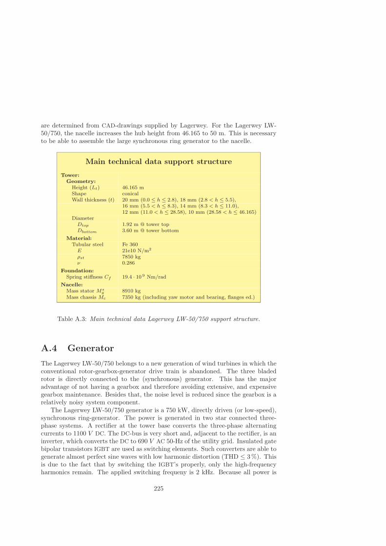
are determined from CAD-drawings supplied by Lagerwey. For the Lagerwey LW-50/750, the nacelle increases the hub height from 46.165 to 50 m. This is necessaryto be able to assemble the large synchronous ring generator to the nacelle.

Main technical data support structure

Tower:Geometry:

Height (Lt) 46.165 mShape conicalWall thickness (t) 20 mm (0.0 ≤ h ≤ 2.8), 18 mm (2.8 < h ≤ 5.5),

16 mm (5.5 < h ≤ 8.3), 14 mm (8.3 < h ≤ 11.0),12 mm (11.0 < h ≤ 28.58), 10 mm (28.58 < h ≤ 46.165)

DiameterDtop 1.92 m @ tower topDbottom 3.60 m @ tower bottom

Material:Tubular steel Fe 360

E 21e10 N/m2

ρst 7850 kgν 0.286

Foundation:Spring stiffness Cf 19.4 · 10 9 Nm/rad

Nacelle:Mass stator Ms

g 8910 kgMass chassis Mc 7350 kg (including yaw motor and bearing, flanges ed.)

Table A.3: Main technical data Lagerwey LW-50/750 support structure.

A.4 Generator

The Lagerwey LW-50/750 belongs to a new generation of wind turbines in which theconventional rotor-gearbox-generator drive train is abandoned. The three bladedrotor is directly connected to the (synchronous) generator. This has the majoradvantage of not having a gearbox and therefore avoiding extensive, and expensivegearbox maintenance. Besides that, the noise level is reduced since the gearbox is arelatively noisy system component.

The Lagerwey LW-50/750 generator is a 750 kW, directly driven (or low-speed),synchronous ring-generator. The power is generated in two star connected three-phase systems. A rectifier at the tower base converts the three-phase alternatingcurrents to 1100 V DC. The DC-bus is very short and, adjacent to the rectifier, is aninverter, which converts the DC to 690 V AC 50-Hz of the utility grid. Insulated gatebipolar transistors IGBT are used as switching elements. Such converters are able togenerate almost perfect sine waves with low harmonic distortion (THD ≤ 3%). Thisis due to the fact that by switching the IGBT’s properly, only the high-frequencyharmonics remain. The applied switching frequeny is 2 kHz. Because all power is

225

rectified to DC and then inverted to AC the generator is decoupled from the utilitygrid, which allows operation at a wide range of speeds [223]. This configurationthus unites the advantages of variable speed (additional energy capture at partialload and potential reduction of fatigue loads on rotor and drive-train) with those ofa grid supply having substatially lower harmonic feedback. The main features aresummarized in Table A.4.

Main technical data generator

General:Rated power (P elec

r ) 750 kWRotor speed

Minimum (nmin) 19 r.p.m.Rated (nr) 27 r.p.m.Maximum (nmax) 36 r.p.m.

Number of pole-pairs (p) 42Number of phases 6Voltage 690 VRated efficiency (ηr

conv) 0.97

Geometry:Diameter

Stator 5.50 m.Rotor 4.90 m.

Airgap between rotor and stator 5±0.5 mm.

Mass:Rotorwheel 14000 kg

Table A.4: Main technical data Lagerwey LW-50/750 generator.

226

Appendix B

Flow states of a wind turbinerotor

In the previous chapters, a wind turbine is assumed to be operating in its intendedstate in which kinetic energy is extracted from the wind. The rotor converts theextracted energy into mechanical energy thereby producing a downwind force whileslowing down the free-stream wind velocity accordingly. This operating state re-quires that the axial induction factor lies between zero and unity. This operatingstate comprises two so-called rotor flow states, notably the windmill and the turbu-lent wake state. Besides these two flow states, a number of other flow states can bedistincted. The axial induction factor a, or equivalently the thrust coefficient Cdax,can be used to characterise these different flow states. The following flow states mayoccur:

• Propellor

• Windmill

• Turbulent wake

• Vortex ring

• Propellor brake

Fig. B.1 indicates these five rotor flow states in the Cdax- a diagram.Wind turbines normally operate in the windmill state, with 0 ≤ a ≤ 0.5. Glauerts

well-known, and well established blade element momentum theory is generally rec-ommended for use in this flow state, resulting in the following relationship betweenthe thrust coefficient and the axial induction factor:

Cdax = 4a(1 − a) (B.1)

This relationship can also be applied for negative axial induction factors (i.e. a < 0).In this so-called propellor state energy is added to the wake thereby producing anupwind force (i.e. Cdax < 0).

227

−0.2 0 0.2 0.4 0.6 0.8 1 1.2 1.4−0.2

0

0.2

0.4

0.6

0.8

1

1.2

1.4

1.6

1.8

a [−]

Cda

x [−

] Propellor Windmill Turbulent wake

Vortex ring

Propellor brake

4a|1−a| →←4a(1−a) →←

♦

♦♦

♦•

• •••• • •

Figure B.1: Thrust coefficient as function of the axial induction factor and cor-responding rotor flow states. Solid curve: momentum theory, dashed curve: mo-mentum theory not valid, dashed-dotted curve: Glauert empirical relation, and , •:measured data [282].

In the turbulent wake state the relationship between the axial induction factorand the thrust coefficient according to the actuator disk/momentum theory has to bereplaced by an empirical relation. The explanation for this is that the momentumtheory predicts a decreasing thrust coefficient with an increasing axial inductionfactor, while data obtained from wind turbines show an increasing thrust coefficient[279] (see Figure B.1). Thus, the momentum theory is considered to be invalidfor axial induction factors larger than 0.5. A number of empirical relations havebeen derived in order to improve agreement between theory and experiment. Theseempirical relations are compared in Fig. 2.1 on page 25 for perpendicular flow. HereGlauert’s empirical model is depicted in order to illustrate that the Cdax- a curvefrom actuator disk/momentum theory fails to describe to measured results for 0.5 <a < 1.0. This is consistent with the fact that the (flow streamline) assumptions onwhich this theory is based are violated in this region.

Wilson and Lissaman extended Eq. (B.1) (knowing that the assumptions areviolated) to the region a > 0.5 in order to understand the observed differencesbetween momentum theory and experimental results. The resulting equation for thethrust coefficient as function of the axial induction factor is as follows:

Cdax = 4a|1 − a| for a > 0.5 (B.2)

When the induction factor is somewhat over unity, the rotor flow state is calledthe vortex ring state. For axial induction factors greater than unity, where the rotorreverses the direction of the flow, the state is termed the propellor brake state. The

228

interested reader is referred to Stoddard [282] for a more comprehensive survey.

229

230

Appendix C

Comparison of the finiteelement, lumped-mass andsuperelement method

In this appendix we will compare exact eigenfrequencies of an Euler-Bernoulli beamwith those of the finite element, lumped-mass and superelement method. In Sec-tion C.1 the exact eigenfrequencies of an Euler-Bernoulli beam are computed. Sec-tion C.2 computes the eigenfrequencies of the finite element approximation. Theeigenfrequencies of the lumped-mass approximation are computed in Section C.3,while those of the superelement approximation are computed in Section C.4. Theapproaches are compared in Section C.5.

C.1 Exact eigenfrequencies

The exact analytical eigenfrequencies are obtained by solving the following frequencyequation (see Section 4.2):

cos(kiL) cosh(kiL) = −1 for i = 1, 2, 3, · · · ,∞The first four non-zero positive roots of this equation are:

k1 ∗ L = 1.875104069k2 ∗ L = 4.694091133k3 ∗ L = 7.854757438k4 ∗ L = 10.99554073

The eigenfrequencies in radians per second corresponding to these values of ki areobtained as

ωi = k2i ·√EI

ρA(C.1)

231

where E the modulus of elasticity, I the area moment of inertia, ρ the mass densityof the material, and A the cross-sectional area of the beam. Hence, the frequencyof vibration of any mode is inversely proportional to square of the length, andproportional to the radius of gyration of the cross-section (i.e.

√I/A). Thus for

geometrically similar beams of the same material, the eigenfrequencies vary in directproportion to the dimensions.

The Euler-Bernoulli beam considered has length L = 50 m, modulus of elasticityE = 21 · 1010 N/m2, area of beam cross-section A = π m2, mass density ρ = 7850kg/m3, and area moment of inertia I = 1

4π m4. The first four exact frequencies arelisted in Table C.1, and will serve as reference solution.

Table C.1: The first four exact eigenfrequencies in radians per second of an Euler-Bernoulli beam with length L = 50 m, a constant flexural rigidity EI of 1.6493 ·1011,a uniformly distributed mass density of 7850 kg/m3, and a cross-sectional area of π.

C.2 Finite Element approximation

In this case, the Euler-Bernoulli beam has been modeled using an increasing numberof finite elements. The elements are 2-noded, elastic straight 3-D beam elementswith 6 degrees of freedom at each node (MARC element type 98). The beam is builtin at the base. The eigenfrequencies were calculated using the Lanczos eigenvalueextraction algorithm. The first four eigenfrequencies are listed in Table C.2.

Table C.2: The first four eigenfrequencies in radians per second of the Finite Elementapproximation as function of the number of finite elements. The singularity ratio isa measure of the reliability of the results. Reliable results are obtained if the ratio islarger than 10−4 and smaller than 1.

232

From this table it can be concluded that the first four modes are represented veryaccurately by 18 finite elements. This model has 36 degrees of freedom (actually 216,but in all fairness we do not count the unused degrees of freedom). The singularityratio (a measure of the reliability of the results; reliable results are obtained if theratio is larger than 10−4 and smaller than 1) indicates that the maximum number ofelements has been reached. Increasing this number any further will result in singularequations (i.e unreliable results), since the cross sectional area - length of elementratio becomes out of proportion.

C.3 Lumped-mass approximation

In this case, the Euler-Bernoulli beam has been modeled by discretizing it in nequally spaced particles (i.e. lumped-masses) connected by joints with springs. InFig. C.1 this is schematically depicted. Again, the beam is built in at the base.The mass of the lumped-masses has been determined by identifying a portion of thebeam such that the inertia effects are modeled by the discrete beam [133].

Figure C.1: Fixed-free Euler-Bernoulli beam discretized with n equally spaced parti-cles (lumped-masses).

The resulting eigenfrequencies of the lumped-mass approximation as function ofthe number of lumped-masses can be found in Kelly [133]. We use only the first foureigenfrequencies which are repeated in Table C.3. The pattern is clear: dividing theEuler-Bernoulli beam into more lumped-masses produces more eigenfrequencies, andimproves the accuracy. The limiting case being an infinite number of lumped-massesof which the eigenfrequencies equal to those of the exact solution.

Table C.3: The first four eigenfrequencies in radians per second of the lumped-massapproximation as function of the number of lumped masses.

233

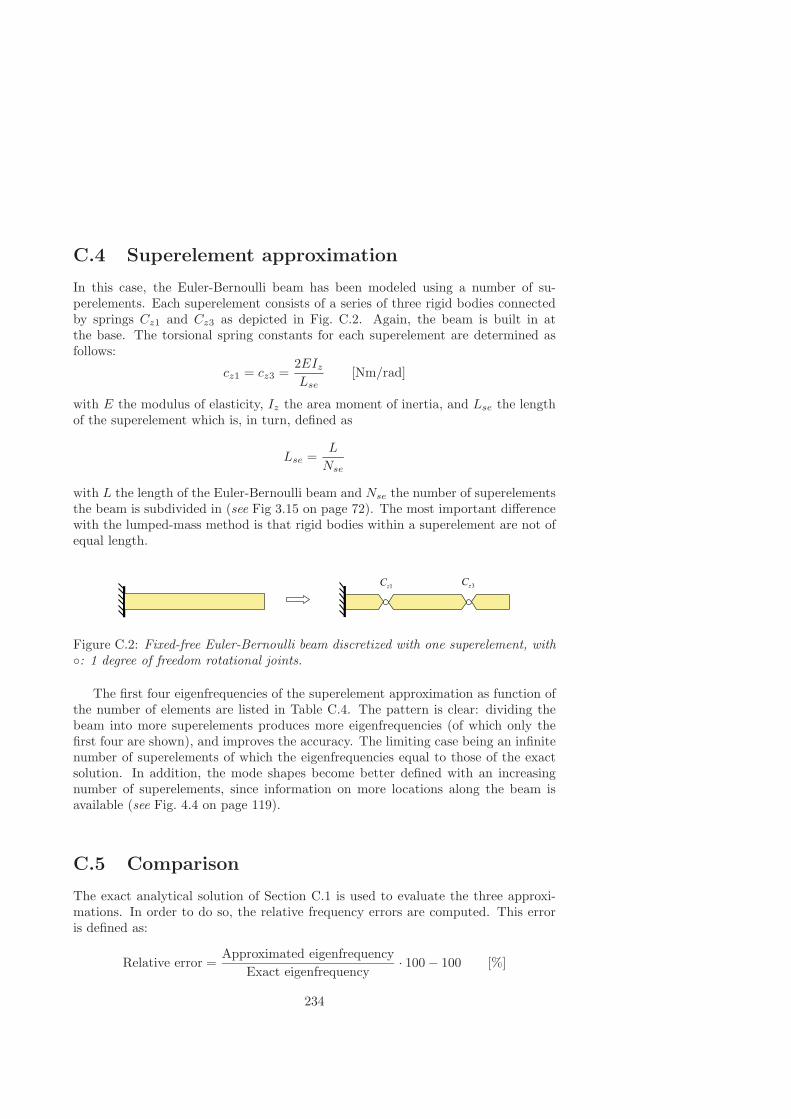
C.4 Superelement approximation

In this case, the Euler-Bernoulli beam has been modeled using a number of su-perelements. Each superelement consists of a series of three rigid bodies connectedby springs Cz1 and Cz3 as depicted in Fig. C.2. Again, the beam is built in atthe base. The torsional spring constants for each superelement are determined asfollows:

cz1 = cz3 =2EIzLse

[Nm/rad]

with E the modulus of elasticity, Iz the area moment of inertia, and Lse the lengthof the superelement which is, in turn, defined as

Lse =L

Nse

with L the length of the Euler-Bernoulli beam and Nse the number of superelementsthe beam is subdivided in (see Fig 3.15 on page 72). The most important differencewith the lumped-mass method is that rigid bodies within a superelement are not ofequal length.

Figure C.2: Fixed-free Euler-Bernoulli beam discretized with one superelement, with: 1 degree of freedom rotational joints.

The first four eigenfrequencies of the superelement approximation as function ofthe number of elements are listed in Table C.4. The pattern is clear: dividing thebeam into more superelements produces more eigenfrequencies (of which only thefirst four are shown), and improves the accuracy. The limiting case being an infinitenumber of superelements of which the eigenfrequencies equal to those of the exactsolution. In addition, the mode shapes become better defined with an increasingnumber of superelements, since information on more locations along the beam isavailable (see Fig. 4.4 on page 119).

C.5 Comparison

The exact analytical solution of Section C.1 is used to evaluate the three approxi-mations. In order to do so, the relative frequency errors are computed. This erroris defined as:

Relative error =Approximated eigenfrequency

Exact eigenfrequency· 100 − 100 [%]

234

Table C.4: The first four eigenfrequencies in radians per second of the superelementapproximation as function of the number of superelements.

The relative errors for the first four eigenfrequencies of both the finite elementand superelement approximation are plotted as function of the number of degrees offreedom in Fig. C.3. Notice that the number of degrees of freedom Ndof are relatedto the number of superelements Nse as follows:

Ndof = 2Nse

0 5 10 15 20 25 30 35 40−5

0

5

10

15

20

Degrees of freedom [−]

Rel

ativ

e er

ror

[%

]

+ 1%

− 1%

Finite element method

Superelement method

Figure C.3: The relative errors for the first four eigenfrequencies of the finite elementand superelement approximation as function of the number of degrees of freedom.Solid line: first mode, dashed line: second mode, dashed-dotted line: third mode,dotted line: fourth mode, and dashed-dotted horizontal lines: + 1% and - 1% errorbound respectively.

The finite element errors are all positive (i.e. the eigenfrequencies are overesti-mated by the finite element model implying that the model is stiffer than the realsystem), and decrease monotonically with an increasing number of finite elements.

235

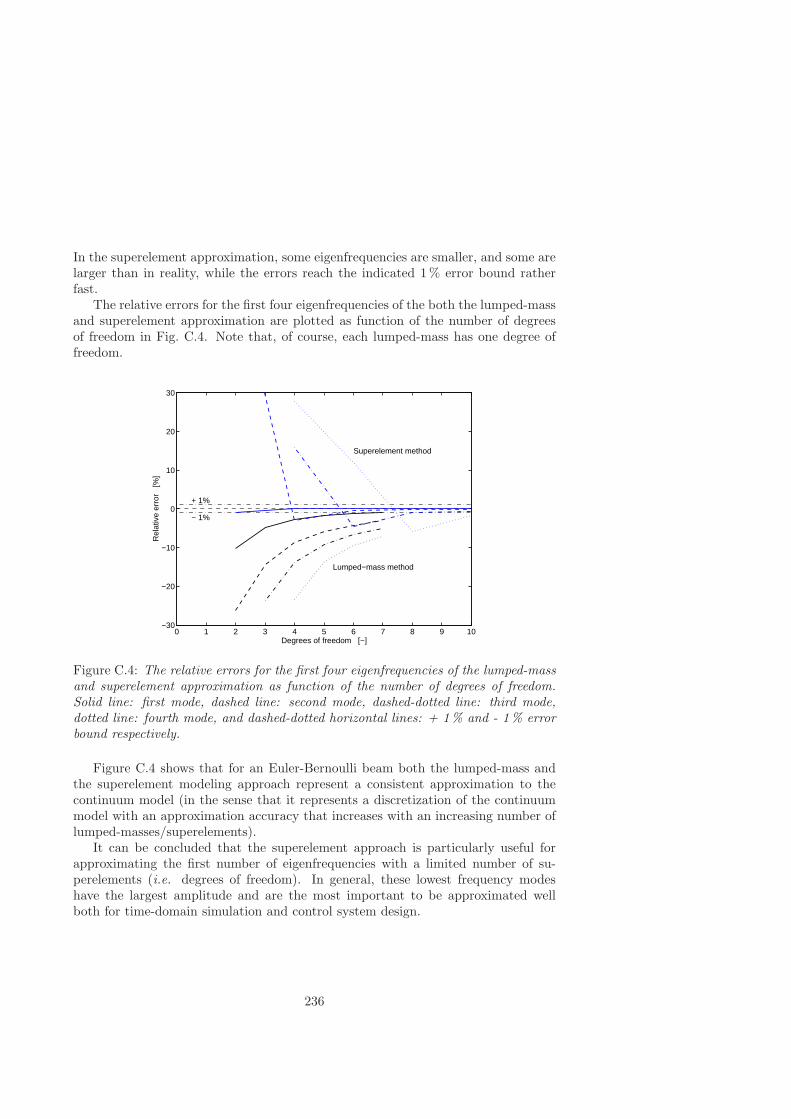
In the superelement approximation, some eigenfrequencies are smaller, and some arelarger than in reality, while the errors reach the indicated 1 % error bound ratherfast.

The relative errors for the first four eigenfrequencies of the both the lumped-massand superelement approximation are plotted as function of the number of degreesof freedom in Fig. C.4. Note that, of course, each lumped-mass has one degree offreedom.

0 1 2 3 4 5 6 7 8 9 10−30

−20

−10

0

10

20

30

Degrees of freedom [−]

Rel

ativ

e er

ror

[%

]

+ 1%

− 1%

Lumped−mass method

Superelement method

Figure C.4: The relative errors for the first four eigenfrequencies of the lumped-massand superelement approximation as function of the number of degrees of freedom.Solid line: first mode, dashed line: second mode, dashed-dotted line: third mode,dotted line: fourth mode, and dashed-dotted horizontal lines: + 1% and - 1% errorbound respectively.

Figure C.4 shows that for an Euler-Bernoulli beam both the lumped-mass andthe superelement modeling approach represent a consistent approximation to thecontinuum model (in the sense that it represents a discretization of the continuummodel with an approximation accuracy that increases with an increasing number oflumped-masses/superelements).

It can be concluded that the superelement approach is particularly useful forapproximating the first number of eigenfrequencies with a limited number of su-perelements (i.e. degrees of freedom). In general, these lowest frequency modeshave the largest amplitude and are the most important to be approximated wellboth for time-domain simulation and control system design.

236

Appendix D

Proofs of Section 3.5

This appendix contains the proofs of the elimination of the non measurable variablesin the stator flux equations of Section 3.5. In Section D.1 both Eq. (3.99) andEq. (3.100) are proven. In Section D.2 Eq. (3.101) is proven.

D.1 Direct-axis

The equation for the field winding voltage, and the equation for the voltage acrossthe direct-axis damper are given by

Uf = RfIf + sΨf (D.1)0 = −R1dI1d − sΨ1d (D.2)

and the flux linkage equations on the direct-axis are given by

Ψd = LdId + kMfIf + kM1dI1d (D.3)Ψf = kMfId + LfIf +MrI1d (D.4)

Ψ1d = kM1dId +MrIf + L1dI1d (D.5)

Substituting Eq. (D.5) in Eq. (D.2) gives

0 = −R1dI1d − s kM1dId +MrIf + L1dI1d

Rearranging leads to

I1d (1 + τ1d s) = −s(kM1d

R1d

)Id − s

(Mr

R1d

)If (D.6)

withτ1d =

L1d

R1d

the rotor time constant for the direct-axis.

237

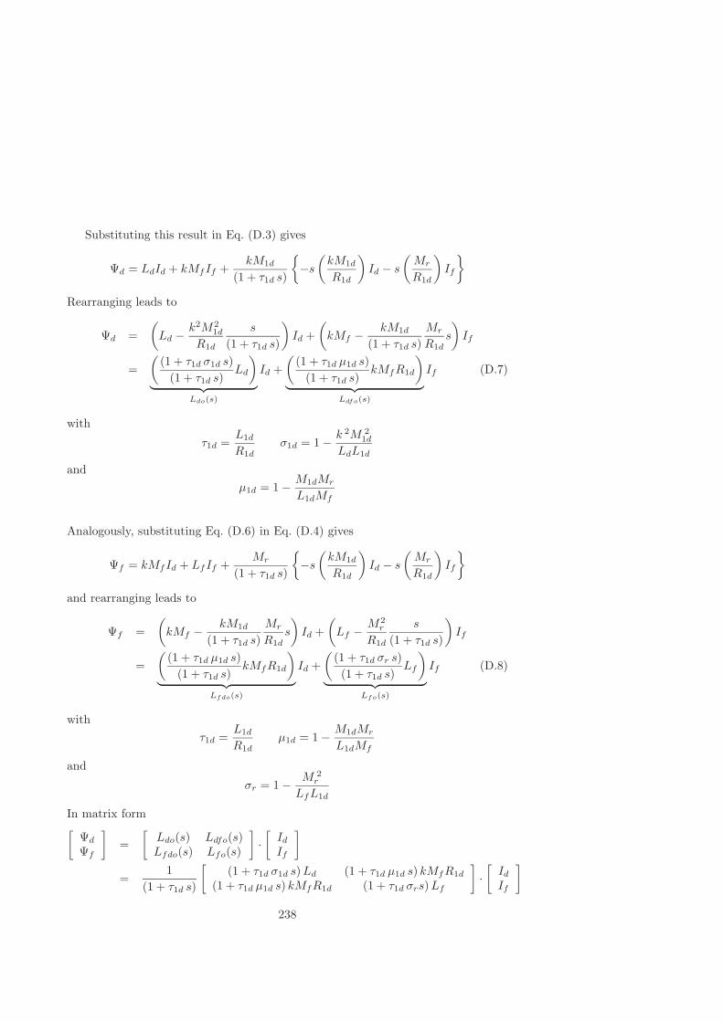
Substituting this result in Eq. (D.3) gives

Ψd = LdId + kMfIf +kM1d

(1 + τ1d s)

−s(kM1d

R1d

)Id − s

(Mr

R1d

)If

Rearranging leads to

Ψd =(Ld − k2M2

1d

R1d

s

(1 + τ1d s)

)Id +

(kMf − kM1d

(1 + τ1d s)Mr

R1ds

)If

=(

(1 + τ1d σ1d s)(1 + τ1d s)

Ld

)︸ ︷︷ ︸

Ldo(s)

Id +(

(1 + τ1d µ1d s)(1 + τ1d s)

kMfR1d

)︸ ︷︷ ︸

Ldfo(s)

If (D.7)

with

τ1d =L1d

R1dσ1d = 1 − k 2M 2

1d

LdL1d

andµ1d = 1 − M1dMr

L1dMf

Analogously, substituting Eq. (D.6) in Eq. (D.4) gives

Ψf = kMfId + LfIf +Mr

(1 + τ1d s)

−s(kM1d

R1d

)Id − s

(Mr

R1d

)If

and rearranging leads to

Ψf =(kMf − kM1d

(1 + τ1d s)Mr

R1ds

)Id +

(Lf − M2

r

R1d

s

(1 + τ1d s)

)If

=(

(1 + τ1d µ1d s)(1 + τ1d s)

kMfR1d

)︸ ︷︷ ︸

Lfdo(s)

Id +(

(1 + τ1d σr s)(1 + τ1d s)

Lf

)︸ ︷︷ ︸

Lfo(s)

If (D.8)

withτ1d =

L1d

R1dµ1d = 1 − M1dMr

L1dMf

and

σr = 1 − M 2r

LfL1d

In matrix form[Ψd

Ψf

]=

[Ldo(s) Ldfo(s)Lfdo(s) Lfo(s)

]·[IdIf

]

=1

(1 + τ1d s)

[(1 + τ1d σ1d s)Ld (1 + τ1d µ1d s) kMfR1d

(1 + τ1d µ1d s) kMfR1d (1 + τ1d σrs)Lf

]·[IdIf

]

238

A few observations can be made. The most important one is that the denom-inators of Ldo(s), Ldfo(s), Lfdo(s), and Lfo(s) are all the same. In addition, thenominators of Ldfo(s) and Lfdo(s) are identical. Consequently,

Ldfo(s) = Lfdo(s) (D.9)

with a DC-gain of kMfR1d. In this thesis this DC-gain is referred to as LDCfdo (or

LDCdfo ). Furthermore, the DC-gain of Ldo(s) is equal to that of Ld(s) and is referred

to as LDCd . Finally, the DC-gain of Lfo(s) is equal to Lf and is referred to as LDC

fo .

The aforementioned conclusion that the denominators of Ldo(s), Ldfo(s), Lfdo(s),and Lfo(s) are identical is valid only for the case that one damper winding is locatedon the direct-axis. Below we will show that this conclusion can be generalized forn damper windings. Consider the n equations for the voltage across the direct-axisdampers:

0 = −R1dI1d − sΨ1d

0 = −R2dI2d − sΨ2d

... =...

...0 = −RndInd − sΨnd

In matrix form

000...0

= −

R1d 0 0 · · · 00 R2d 0 · · · 00 0 R3d · · · 0...

......

. . ....

0 0 0 · · · Rnd

·I1d

I2d

I3d

...Ind

−s 0 0 · · · 00 s 0 · · · 00 0 s · · · 0...

......

. . ....

0 0 0 · · · s

·

Ψ1d

Ψ2d

Ψ3d

...Ψnd

The corresponding direct-axis and field winding flux linkage equations are given by

Ψd = LdId + kMfIf + kM1dI1d + kM2dI2d + · · · + kMndInd

Ψf = kMfId + LfIf +M1rI1d +M2rI2d + · · · +MnrInd

while the damper winding flux linkage equations are given by

Ψ1d = kM1dId +M1rIf + L1dI1d +M1d2dI2d + · · · +M1dndInd

Ψ2d = kM2dId +M2rIf + L2dI2d +M2d1dI1d + · · · +M2dndInd

... =...

......

......

...Ψnd = kMndId +MnrIf + LndInd +Mnd1dI1d + · · · +Mndnd−1Ind−1

withMidjd = Mjdid for i = j

239

In matrix form

Ψ1d

Ψ2d

Ψ3d

...Ψnd

=

kM1d M1r L1d M1d2d M1d3d · · · M1dnd

kM2d M2r M1d2d L2d M2d3d · · · M2dnd

kM3d M3r M1d3d M2d3d L3d · · · M3dnd

......

......

.... . .

...kMnd Mnr M1dnd M2dnd M3dnd · · · Lnd

·

IdIfI1d

I2d

I3d

...Ind

The derivation of Ψd = f(Id, If ) and Ψf = f(Id, If ) via substitution and rear-ranging of the aforementioned equations is very time-consuming with pen and paper.Therefore, we have decided to use the mathematical manipulation package MAPLE V[45] to symbolically determine the aforementioned expressions. Next, the If and Idcomponents are extracted from Ψd = f(Id, If ) and Ψf = f(Id, If ). Subsequently,the numerators and denominators of both Ldo(s)/Lfdo(s) and Ldfo(s)/Lfo(s) are de-termined. Finally, the four denominators and the numerators of Lfdo(s) and Ldfo(s)are compared in order to check the general conclusion.

For example, consider the case where two damper windings are located on thed-axis (i.e. n = 2):

%

% Maple V input:

%

%

% Psid:

%

eq1:= -R1d*I1d-s*Psi1d=0:

eq2:= -R2d*I2d-s*Psi2d=0:

eq3:= k*M1d*Id+M1r*If+L1d*I1d+M1d2d*I2d=Psi1d:

eq4:= k*M2d*Id+M2r*If+L2d*I2d+M1d2d*I1d=Psi2d:

eq5d:= Ld*Id+k*Mf*If+k*M1d*I1d+k*M2d*I2d=Psid:

%

SolutionSetPsid:=solve(eq1,eq2,eq3,eq4,eq5d,Psi1d,I1d,Psi2d,I2d,Psid);

%

% Select Psid from SolutionSet:

%

% --> Psid = (Ld*Id*R1d*R2d+Ld*Id*R1d*s*L2d+ ...

% +k*M2d*s^2*M1r*If*M1d2d) / ...

% (R1d*R2d+R1d*s*L2d+s*L1d*R2d+s^2*L1d*L2d-s^2*M1d2d^2)

%

op(3,SolutionSetPsid);

%

% --> Psid = ...

%

240

Psid:=(...);

Psid:=collect(Psid,[Id,If]);

%

% Extract Ldo(s)*Id and Ldfo(s)*If from expression:

%

Ldo:=op(1,Psid);

Ldfo:=op(2,Psid);

%

% Compute numerators and denominators:

%

num_LdoId:=numer(Ldo);

nops_LdoId:=nops(num_LdoId);

%

% --> nops_LdoId:= 2

%

num_Ldo:=op(nops(num_LdoId)-1,num_LdoId);

den_Ldo:=denom(Ldo);

num_LdfoIf:=numer(Ldfo);

nops_LdfoIf:=nops(num_LdfoIf);

%

% --> nops_LdfoIf:= 3

%

num_Ldfo:=op(nops_LdfoIf-1,num_LdfoIf)*op(nops_LdfoIf-2,num_LdfoIf);

den_Ldfo:=denom(Ldfo);

%

%

%

%

% Psif:

%

eq5f:= k*Mf*Id+Lf*If+M1r*I1d+M2r*I2d=Psif:

%

SolutionSetPsif:=solve(eq1,eq2,eq3,eq4,eq5f,Psi1d,I1d,Psi2d,I2d,Psif);

%

% Select Psif from SolutionSet:

%

op(3,SolutionSetPsif);

%

% --> Psif = ...

%

Psif:=(...);

Psif:=collect(Psif,[Id,If]);

241

%

% Extract Lfdo(s)*Id and Lfo(s)*If from expression:

%

Lfdo:=op(1,Psif);

Lfo:=op(2,Psif);

%

% Compute numerators and denominators:

%

num_LfdoId:=numer(Lfdo);

nops_LfdoId:=nops(num_LfdoId);

%

% --> nops_LfdoId:= 3

%

num_Lfdo:=op(nops(num_LfdoId)-2,num_LfdoId)*op(nops(num_LfdoId)-1,num_LfdoId);

den_Lfdo:=denom(Lfdo);

num_LfoIf:=numer(Lfo);

nops_LfoIf:=nops(num_LfoIf);

%

% --> nops_LfoIf:= 2

%

num_Lfo:=op(nops(num_LfoIf)-1,num_LfoIf);

den_Lfo:=denom(Lfo);

%

% Check whether denominators and numerators are identical:

%

(den_Ldo-den_Ldfo)-(den_Lfdo-den_Lfo);

(num_Ldfo-num_Lfdo);

%

%

%

Investigation has shown that the four denominators as well as the numerators ofLdfo and Lfdo are identical at least till 4 damper windings. Due to similarity, it isexpected that this conclusion holds for a finite number of damper windings.

D.2 Quadrature-axis

The equation for the voltage across the quadrature-axis damper is given by

0 = −R1qI1q − sΨ1q (D.10)

and the flux linkage equations on the quadrature-axis are given by

Ψq = LqIq + kM1qI1q (D.11)Ψ1q = kM1qIq + L1qI1q (D.12)

242

Rearranging Eq. (D.11) gives

I1q =Ψq − LqIqkM1q

(D.13)

Substituting this result in Eq. (D.12) gives

Ψ1q = kM1qIq + L1q

Ψq − LqIqkM1q

(D.14)

Substituting Eq. (D.13) and Eq. (D.14) in Eq. (D.10) gives

0 = −R1q

Ψq − LqIqkM1q

− s

kM1qIq + L1q

(Ψq − LqIqkM1q

)(D.15)

Rearranging Eq. (D.15) gives

Ψq

R1q

kM1q+

sL1q

kM1q

=

R1qLq

kM1q

Iq − skM1q Iq +

sL1qLq

kM1q

Iq

Ψq

1 +

L1q

R1q· s

=

Lq −

s k2M21q

R1q+sL1qLq

R1q

Iq

= LqIq

1 +

L1q

R1q· s− k2M2

1q

R1q

1Lq

· s

= LqIq

1 +L1q

R1q︸︷︷︸τ1q

(1 − k 2M 2

1q

LqL1q

)︸ ︷︷ ︸

σ1q

·s

(D.16)

with τ1q the rotor time constant for the quadrature-axis and σ1q the leakage factor.Rearranging the above equation leads to

Ψq = LqIq1 + τ1qσ1q · s

1 + τ1q · s=

(Lq

1 + τ1qσ1q · s1 + τ1q · s

)︸ ︷︷ ︸

Lq(s)

·Iq

243

244

Appendix E

Main wind turbine modes ofoperation

In this chapter the main wind turbine modes of operation will be discussed. Ingeneral, the following modes of operation can be distinguished [179]:

• Startup

• Power generation

• Shutdown

• Emergency

In the startup mode the rotor of the wind turbine is accelerated, and the generatoris connected to the utility grid.

In the power generation mode, power is extracted from the wind and converted toelectricity. In this mode the wind velocity ranges from the cut-in wind velocity Vci,via the rated velocity Vr to the cut-out wind velocity Vco as illustrated in Fig. E.1 fora fictive variable rotational speed wind turbine. For the purpose of illustration, thevalues for Vci, Vr and Vco are 3.0, 12.5 and 25.0 m/s respectively for the LagerweyLW-50/750. In the power generating mode, two different operating areas can bedistinguished, viz. partial load (Vci < Vw ≤ Vr) and full load (Vr ≤ Vw < Vco)[36]. In partial load, the aerodynamic (or rotor) power is proportional to the cubicwind velocity. In this operating area maximum energy capture can be achieved bytracking the optimum tip-speed ratio curve (i.e. the λopt-curve). Above the ratedwind velocity the aerodynamic power P (and by that the rated generator power) iskept at a constant level: Pr. This is a given fact from generator design, in what,among other things, the wind regime, heat rise and loads acting on the constructionare considered. This can be achieved either by stall or, in case of adjustable blades,by pitching the rotor blades towards a smaller (i.e. feathering control) or largerangle of attack (active stall control). In Molenaar [188] it has been concluded thati) adjustable blades are preferred to blades with a fixed pitch angle (despite the

245

higher initial costs), and ii) pitching the blades towards a smaller angle of attack ispreferred to active stall control.

V V V

P

P

P

[kW

]

Vw [m/s]

ci r co

ci

r

→←Full load

λ = λopt

← →Partial load

Figure E.1: Rotor power (P ) as a function of the undisturbed wind velocity (Vw) of afictive variable rotational speed wind turbine, with Vci: cut-in wind velocity, Vr: ratedwind velocity, Vco: cut-out wind velocity, Pci: start power, Pr: rated aerodynamicpower, and λ: tip-speed ratio.

In the shutdown mode the generator is disconnected and the turbine is deceler-ated. The system is in an emergency mode if a serious malfunction has been detected(e.g. failed pitch mechanism). If happens, the backup systems are invoked by thesupervisory control system to provide for a safe shutdown.

246

Appendix F

Modal analysis measurementequipment

This appendix describes the measurement equipment used in the “modal analysis”.Section F.1 lists the main specifications of the cable used to excite the Lagerwey LW-50/750 wind turbine. The main features of the data acquisition system are presentedSection F.2. Section F.3 lists the main specifications of the force transducer. Finally,Section F.4 presents the specifications as well as locations of the accelerometers used.

F.1 Cable

The static load is applied to the tower by a 225 meter long TWARON R© cable an-chored a 20-ton winch truck using a pin joint (see Fig. F.1). TWARON R© is alightweight, superstrong synthetic fiber made from the aramid polymer. The ca-ble has a tensile strength of 170 kN and a total mass of 82.5 kg (i.e. includingpin joints). The interested reader is referred to the homepage of Twaron ProductsV.o.F. (www.twaron.com) for detailed information about TWARON R©.

Figure F.1: Detail of the TWARON cable and pin joint.

247

F.2 Data acquisition system

Two supervisory control and data acquisition systems (SCADAS II) of Leuven Mea-surement Systems (LMS) with each 24 channels are used to store the time-domainas well as frequency domain data [249]. The name plate data of both SCADAS arelisted in Fig. F.2.

Figure F.2: Name plate data of LMS-DIFA SCADAS II data acquisition system.

The programmable dual filter amplifier (PDFA) module in the LMS-DIFA SCA-DAS II is a universal signal conditioning module providing two identical, but eachindependently programmable differential amplifiers and analogue anti-aliasing fil-ters. The PDFA includes a current source to provide power to integrated circuitpiezoelectric transducers.

Five commonly used types of analogue filters are Butterworth, Elliptic, Cheby-shev (Type I and II), and Bessel. These so-called infinite impulse response (IIR)filters all approximate the ideal filter in different ways. Note that an ideal low-passfilter would have no attenuation in the pass band (i.e. 0 < f < fco), infinite atten-uation in the stopband (i.e. f > fco), and a zero phase characteristic. In practice,a linear phase characteristic is often regarded as “ideal”. After all, a linear phasecharacteristic introduces a time shift but preserves the wave shapes. Of the fivementioned filter types, elliptic filters usually meet a given set of filter performancespecifications with the lowest filter order.

The PDFA anti-aliasing filters are eighth-order elliptic filters. They are builtup by cascading four identical second order filter stages to approximate the idealfilter. Three filter characteristics are available, viz. PDFA-ETD (Equal Time Delay),PDFA-ELL (Elliptical), and PDFA-US (Ultra Sharp). We have used the PDFA-ETDanti-aliasing filter. The cutoff frequency fco of this filter can be varied from 10 Hzto 10.23 kHz in 10 Hz steps to meet the sample frequency and frequency range ofinterest requirements. The ETD filter uses 8 poles and 8 zeros to approximate theideal filter. The result is a linear phase response within 2.2 while the stopbandattenuation of 70 dB is reached at 3.7 · fco. The Bode diagram of this filter isdepicted in Fig. F.3.

The sampling and quantisation is carried out by a 16-bit A/D converter. Theaccuracy of the sampling and quantisation process depends on the number of quan-tisation levels available in the A/D converter (an n-bit converter has 2n quantisationlevels). In practice, the measured signal should occupy as much of the range of the

248

0 0.1 0.2 0.3 0.4 0.5 0.6 0.7 0.8 0.9 10.7

0.8

0.9

1

Normalised cutoff frequency f/fco

[−]

Mag

nitu

de

[−]

0 0.1 0.2 0.3 0.4 0.5 0.6 0.7 0.8 0.9 1−200

−150

−100

−50

0

Normalised cutoff frequency f/fco

[−]

Pha

se

[Deg

rees

]

Figure F.3: Amplitude and phase characteristic of the Equal Time Delay anti-aliasing filter as a function of the normalised cutoff frequency f/fco. Dashed line:ideal low-pass filter with phase proportional to f/fco.

A/D converter as possible. Provided that is done, quantisation errors are normallyinsignificant [170, 265]. The data were collected with a sample rate of 1000 Hz (mea-surement M1) and 500 Hz (measurement M2-M10), and with the cutoff frequency ofthe ETD low-pass filter set to 330 and 160 Hz respectively.

F.3 Force transducer

The magnitude of the input force is measured in-line with the cable between thequick release mechanism and the winch truck using a force transducer. The nameplate data of the force transducer is listed in Fig. F.4.

Figure F.4: Name plate data of the force transducer.

249

F.4 Accelerometers

Three types of accelerometers are used, viz. Endevco model 2262A-25, Endevcomodel 2262A-200, and Sundstrand model QA-700. The Endevco accelerometersare rugged, fluid damped transducers of the piezoresistive type. The output rangeof model 2262A-25 is ± 25 g, and of model 2262A-200 ± 200 g. Both models arelight weight (28 gram), high-sensitivity (20 mV/g and 2.5 mV/g respectively at100 Hz). The static acceleration limit is 250 g for model 2262A-25 and 1000 g formodel 2262A-200. The frequency range of model 2262A-25 is from 0 to 650 Hz andof model 2262A-200 from 0 to 1800 Hz. Detailed technical data can be found atwww.endevco.com.

The integral electronics in the Sundstrand accelerometers develop an acceleration-proportional output current providing both static and dynamic acceleration mea-surements. They have an output range of ± 30 g and a maximum bias of 8·10−3

g. The static acceleration limit is 250 g. The Sundstrand accelerometers weigh 46grams. Detailed technical data can be found at www.inertialsensor.com.

The high-sensitivity of both the Endevco and Sundstrand accelerometers is idealfor obtaining good signal-to-noise ratio even when the response amplitudes are low.

F.4.1 Accelerometer mounting

For an accelerometer to generate accurate and useful data, it must be properlycoupled to the system under investigation. This means that the mounting must berigid over the frequency range of interest to avoid distortion of the frequency responseof the measurement. The natural frequency of an accelerometer, when mounted, isdependent on the stiffness of the coupling method. This requires a proper selectionof the accelerometer mounting technique to be applied as well as thorough surfacepreparation. The following mounting methods are commonly used:

• Threaded studs;

• Adhesives (e.g. hot glue, double-back tape, and cyanoacrylate);

• Magnetic adapters.

The key question is which mounting method is most suited for the intended purpose.The recommended mounting method is that used for calibration [177]. Issues thatmust be considered include: weight of the accelerometer, required bandwidth of themeasurement, amplitude anticipated, type of mounting surface, and whether or nota mounting surface may be altered.

When possible, the best method is to mount an accelerometer with a stud sinceno adhesive is as stiff as a mounting stud. Cyanoacrylate instant adhesives have thewidest frequency range and the broadest temperature limits of the adhesive-mountoptions for accelerometers weighing less than 10 grams, but attachment on roughsurfaces is difficult and removal is time consuming [178]. Double back tape and hotglue are viable alternatives when removal time is an important issue. Hot glue is thepreferred method of attachment for systems having hard to reach areas. Magnetic

250

mounting is convenient and easily accomplished for accelerometers weighing over 50grams. This method, however, reduces the usable bandwidth.

In our case it was not allowed to tap holes into the tower and rotor blades fora stud mount. We have decided to mount the accelerometers on the blades withhot glue (for easy attachment and removal) and to mount the accelerometers on thetower with double-back tape.

F.4.2 Accelerometer positions

The accelerometer positions are listed in Table F.1. The tower postions are measuredwith respect to the ground level, the blade postions are measured with respect tothe blade tips.

Accelerometers

Tag Position Tower/Blade Orientation Type

A-01 0.00 Tower – (x) QA-700A-02 12.66 Tower – (x) QA-700A-03 21.80 Tower – (x) QA-700A-04 36.00 Tower – (x) QA-700A-05 44.38 Tower – (x) QA-700

A-06 13.75 Blade A L1 (z) 2262A-25A-07 13.75 Blade A D1 (x) 2262A-25A-08 7.75 Blade A L1 (z) 2262A-200A-09 7.75 Blade A D1 (x) 2262A-200A-10 7.75 Blade A D2 (x) 2262A-200A-11 1.75 Blade A L1 (z) 2262A-200A-12 1.75 Blade A D1 (x) 2262A-200A-13 1.75 Blade A D2 (x) 2262A-200

A-14 1.75 Blade B L1 (z) 2262A-200A-15 1.75 Blade B D1 (x) 2262A-200A-16 1.75 Blade B D2 (x) 2262A-200

A-17 1.75 Blade C L1 (z) 2262A-200A-18 1.75 Blade C D1 (x) 2262A-25A-19 1.75 Blade C D2 (x) 2262A-25

Table F.1: Accelerometer positions on both the tower (w.r.t. ground level) and therotor blades (w.r.t. blade tip). During the parked modal test, blade A is pointingupwards (i.e. at 12 o’clock position) while blade B and C are numbered anti-clockwise(rotation about x-axis).

The orientation of the rotor blade accelerometers is shown in Fig. F.5. The“L1” accelerometers are placed at the rotor blade nose. The “D1” accelerometers

251

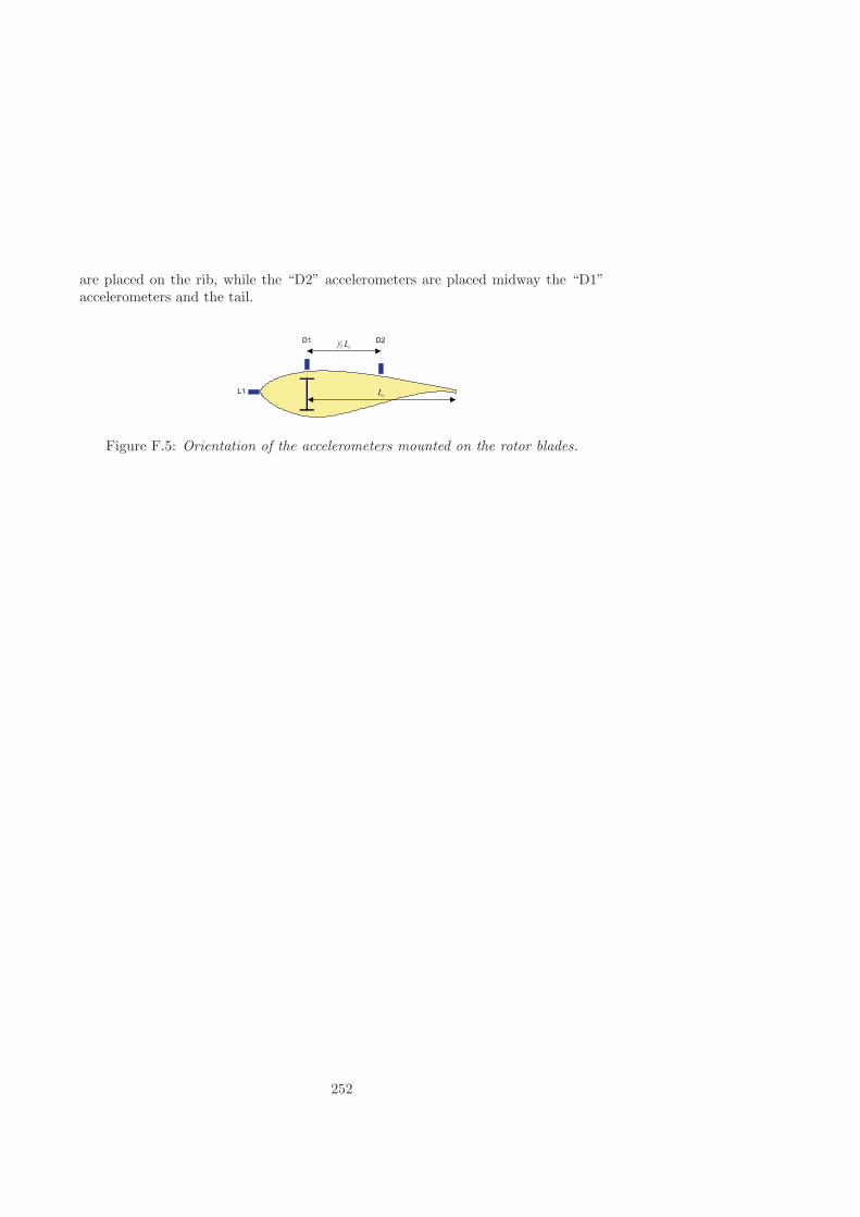
are placed on the rib, while the “D2” accelerometers are placed midway the “D1”accelerometers and the tail.

Figure F.5: Orientation of the accelerometers mounted on the rotor blades.

252

Appendix G

Frequency response functions

This appendix gives a brief review of the main properties of frequency responsefunctions. Section G.1 treats a single degree of freedom system, while Section G.2treats a two degrees of freedom system.

G.1 Single degree of freedom

Consider the single degree of freedom (SDOF) system shown in Fig. G.1. The systemconsists of a rigid body of length L that is free to rotate about the axis of rotation andthat is connected to the ground through a torsional spring. Damping is completelyneglected. For a rigid body in pure rotation about a fixed axis, Newton’s secondlaw of motion states that the sum off all torques about a given axis is equal to theproduct of the mass moment of inertia of a body about that axis and its angularacceleration. Consequently, the equation of motion for the above system can bewritten as

JO θ = MO (G.1)

where JO, θ, and MO are, respectively, the mass moment of inertia about point O,the angle of rotation, and the external moment about O.

Figure G.1: Single degree of freedom system consisting of a rigid body of length Lconnected to the ground by means of a pin joint.

253

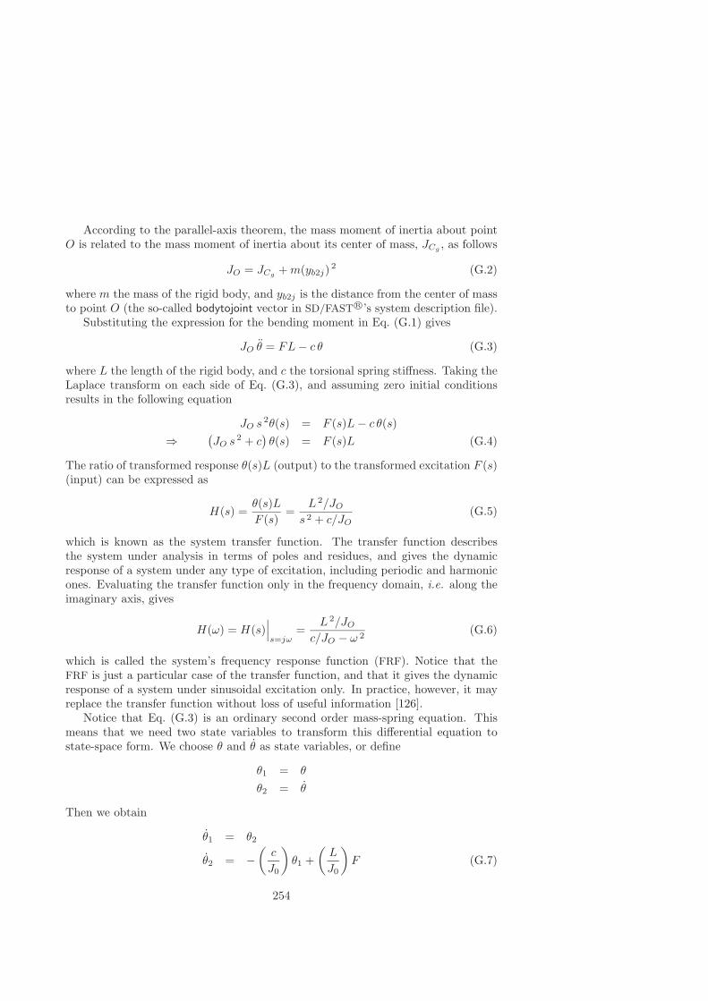
According to the parallel-axis theorem, the mass moment of inertia about pointO is related to the mass moment of inertia about its center of mass, JCg

, as follows

JO = JCg+m(yb2j) 2 (G.2)

where m the mass of the rigid body, and yb2j is the distance from the center of massto point O (the so-called bodytojoint vector in SD/FAST R©’s system description file).

Substituting the expression for the bending moment in Eq. (G.1) gives

JO θ = FL− c θ (G.3)

where L the length of the rigid body, and c the torsional spring stiffness. Taking theLaplace transform on each side of Eq. (G.3), and assuming zero initial conditionsresults in the following equation

JO s2θ(s) = F (s)L− c θ(s)

⇒ (JO s

2 + c)θ(s) = F (s)L (G.4)

The ratio of transformed response θ(s)L (output) to the transformed excitation F (s)(input) can be expressed as

H(s) =θ(s)LF (s)

=L 2/JO

s 2 + c/JO(G.5)

which is known as the system transfer function. The transfer function describesthe system under analysis in terms of poles and residues, and gives the dynamicresponse of a system under any type of excitation, including periodic and harmonicones. Evaluating the transfer function only in the frequency domain, i.e. along theimaginary axis, gives

H(ω) = H(s)∣∣∣s=jω

=L 2/JO

c/JO − ω 2(G.6)

which is called the system’s frequency response function (FRF). Notice that theFRF is just a particular case of the transfer function, and that it gives the dynamicresponse of a system under sinusoidal excitation only. In practice, however, it mayreplace the transfer function without loss of useful information [126].

Notice that Eq. (G.3) is an ordinary second order mass-spring equation. Thismeans that we need two state variables to transform this differential equation tostate-space form. We choose θ and θ as state variables, or define

θ1 = θ

θ2 = θ

Then we obtain

θ1 = θ2

θ2 = −(c

J0

)θ1 +

(L

J0

)F (G.7)

254

The output equation isy = Lθ1 (G.8)

In vector-matrix form, Eq. (G.7) and (G.8) can be written as[θ1θ2

]=

[0 1

− cJ0

0

] [θ1θ2

]+[

0LJ0

]F (G.9)

y =[L 0

] [ θ1θ2

](G.10)

The above equation is in standard state-space form

x = Ax + Bu

y = Cx +Du

where

A =[

0 1− c

J00

], B =

[0LJ0

], C =

[L 0

], D = 0

In structural and control engineering, the frequency response function is graph-ically plotted as log |H(s)| and arg (H(s)) against log(ω), which is called the Bodediagram or Bode plot.

A few observations can be made. Examination of Eq. (G.5) reveals that thenatural frequency of a SDOF system with input and output configuration as selected,is equal to

ωn =√

c

JO=√

c

JCg+m(yb2j) 2

(G.11)

Furthermore, it is clear from Eq. (G.6) that the DC-gain (ω = 0) is equal to L 2/c,while for high frequencies (ω ωn) the asymptote has a slope of -2 on a log-logplot.

Consider a SDOF system consisting of a rigid body with length L = 9 m, distancefrom the center of mass to point O yb2j = 5 m, mass m = 1000 kg, centroidal massmoment of inertia JCg

= 50000 kgm 2, and torsional spring stiffness c = 250000N/m. The receptance, mobility and inertance (or accelerance) Bode plot of thissystem are shown in Fig. G.2. The receptance plot displays the ratio between aharmonic displacement response and the harmonic input force, the mobility plotdisplays the ratio between the velocity response and input force, while the inertance(or accelerance) plot displays the ratio of acceleration response and input force.

The low-frequency asymptote (indicated by the dashed horizontal line in thereceptance plot) intersects the high-frequency asymptote (indicated by the dashedline with a slope of -2 in the receptance plot) at a point corresponding to the naturalfrequency of the system. This is to be expected if we recall that spring force andinertia force cancel when the system is oscillating at its natural frequency (ω = ωn).From this figure it can be concluded that the inertia and stiffness properties alwaysappear as straight lines in a Bode plot. In addition, the mobility plot is symmetricalabout a vertical line passing through the resonance frequency (this is approximatelytrue for lightly damped SDOF systems).

255

10−1

100

101

10−5

100

Receptance

Gai

n [

−]

L2/c

L2/(J0⋅ ω2)

10−1

100

101

−200

−150

−100

−50

0

Frequency [rad/s]

Pha

se

[Deg

rees

]

10−1

100

101

10−5

100

Mobility

ω⋅ L2/c

L2/(J0⋅ ω)

10−1

100

101

−100

−50

0

50

100

Frequency [rad/s]

10−1

100

101

10−6

10−4

10−2

100

Inertance

ω2⋅ L2/c

L2/J0

10−1

100

101

0

50

100

150

200

Frequency [rad/s]

Figure G.2: Bode diagrams (receptance, mobility and inertance) of an undamped,single degree of freedom system (example rigid body with length L = 9 m, distancefrom the center of mass to point O yb2j = 5 m, mass m = 1000 [kg], centroidal massmoment of inertia JCg

= 50000 [kgm 2], and torsional spring stiffness c = 250000[N/m].)

Hence, if Fig. G.2 represented a Bode diagram of experimental data, it would bepossible to derive the torsional spring constant (provided that the length is known),and the mass moment of inertia about O of a SDOF model for the system underanalysis. Damping characteristics can be obtained as well, as will be explained fur-ther on. This reasoning forms the basis of grey-box system identification techniqueswhich aim at deriving the dynamic characteristics from experimental data using aphysical model structure.

If we add a viscous damper to the SDOF system at the pin joint (by specify-ing a coefficient k of viscous damping), the system transfer function from force todisplacement becomes

H(s) =θ(s)LF (s)

=L 2/JO

s 2 + k/JO s+ c/JO(G.12)

and the receptance FRF becomes

H(ω) = H(s)∣∣∣s=jω

=L 2/JO

c/JO + k/JO jω − ω 2(G.13)

=L 2/JO

ω 2n + k/JO jω − ω 2

(G.14)

Observe that the receptance FRF is now (as opposed to the undamped case) acomplex valued function, containing both phase and frequency information.

256

The real and imaginary parts of the receptance, mobility and inertance FRF ofthe viscously damped SDOF system are shown in Fig. G.3. The coefficient k isselected such that the system has a damping ratio of 1 % (i.e. lightly damped). Itis interesting to note that the phase change trough the resonance region is charac-terized by a sign change in one part accompanied by a peak (either a minimum ora maximum) in the other part. From this figure it can be concluded that the recep-tance and inertance frequency response function are, at resonance, purely imaginary,while the mobility FRF is at resonance purely real. This fact can be used to checkthe viscously damped assumption for lightly damped systems.

0 5 10−1

−0.5

0

0.5

1x 10

−3

Rea

l par

t

Receptance

0 5 100

0.5

1

1.5

2

2.5

3x 10

−3 Mobility

0 5 10−2

−1

0

1

2

3

4x 10

−3 Inertance

0 5 10−2

−1.5

−1

−0.5

0x 10

−3

Frequency [rad/s]

Imag

inar

y pa

rt

0 5 10−1.5

−1

−0.5

0

0.5

1

1.5x 10

−3

Frequency [rad/s]0 5 10

0

1

2

3

4

5

6x 10

−3

Frequency [rad/s]

Figure G.3: Plots of real and imaginary parts of the frequency response functionsof a viscously damped, single degree of freedom system (example rigid body withlength L = 9 m, distance from the center of mass to point O yb2j = 5 m, massm = 1000 [kg], centroidal mass moment of inertia JCg

= 50000 [kgm 2], torsionalspring stiffness c = 250000 [N/m] and damping k = 27500 [kg/s].)

G.2 Two degrees of freedom

Consider the two degrees of freedom (2-DOF) system shown in Fig. G.4. The systemconsists of three rigid bodies connected by two ideal torsional springs Cz1 and Cz3

that model the elastic properties in bending direction. The damping is modeled bytwo viscous dampers, Keq12 and Keq23 respectively. The input is the force F and theoutput is the displacement of the point action of F . Gravity is completely neglected.

The equations of motion of the above (2-DOF) system can be solved more easilyusing Lagrange’s equations than using Newton’s law directly as in Section G.1. The

257

Figure G.4: Two degrees of freedom system (superelement) of length Lse consistingof three rigid bodies with lengths 1

2 (1 − 1√3) · Lse, 1√

3· Lse, and 1

2 (1 − 1√3) · Lse.

Lagrange formulation states that the equations of motion can be derived from

d

dt

(∂T

∂qi

)−(∂T

∂qi

)+(∂U

∂qi

)= Qi i = 1, 2, · · · , n (G.15)

where qi = ∂qi/∂t is the generalized velocity, T is the kinetic energy of the system,U the potential energy of the system, an Qi represents all the nonconservative forcescorresponding to qi. Here ∂/∂qi denotes the partial derivative with respect to thecoordinate qi. For conservative systems, Qi = 0 and Eq. (G.15) reduces to

d

dt

(∂T

∂qi

)−(∂T

∂qi

)+(∂U

∂qi

)= 0 i = 1, 2, · · · , n (G.16)

Equations (G.15) and (G.16) represent one equation for each generalized coordi-nate. These equations can be rewritten in a slightly simplified form by defining theLagrangian, L, to be L = T − U , the difference between the kinetic and potentialenergies. Then if ∂U/qi = 0, the Lagrangian equation becomes

d

dt

(∂L

∂qi

)−(∂L

∂qi

)= 0 i = 1, 2, · · · , n (G.17)

Notice that Eq. (G.17) is just a restatement of Newton’s law in generalized coordi-nates ( d

dt (momentum) = applied force).The equations of motion of the two degrees of freedom system in Fig. G.4 can

be described by the two independent coordinates θ1 and θ2, so a good choice of thegeneralized coordinates is q1(t) = θ1(t) and q2(t) = θ2(t). Letting r1 and r2 be thedistance from the joints to the center of mass and l1 and l2 the length for each rigidbody, as shown in the figure, we have for rigid body 1

x1 = r1 sin q1y1 = r1 cos q1x1 = r1q1 cos q1y1 = −r1q1 sin q1

258

and for rigid body 2 we have

x2 = l1 sin q1 + r2 sin(q1 + q2)y2 = l1 cos q1 + r2 cos(q1 + q2)x2 = l1q1 cos q1 + r2(q1 + q2) cos(q1 + q2)y2 = −l1q1 sin q1 − r2(q1 + q2) sin(q1 + q2)

For rigid body 1 the kinetic and potential energy becomes

T1 = 12m1(x2

1 + y21) + 1

2J1q21

= 12m1r

21 q

21 + 1

2J1q21

U1 = 12Cz1q

21

where m1 the mass, and J1 the mass moment of inertia about the center of mass ofrigid body 1. The velocity squared of the center of gravity of rigid body 2 is

x22 + y2

2 = l21 q21 + r22(q1 + q2)2 + 2l1r2(q21 + q1q2) cos q2

Therefore the expression for kinetic energy for rigid body 2 is

T2 = 12m2(x2

2 + y22) + 1

2J2(q1 + q2)2

= 12m2l

21 q

21 + 1

2m2r22(q1 + q2)2 +m2l1r2(q21 + q1q2) cos q2 + 1

2J2(q1 + q2)2

The potential energy isU2 = 1

2Cz3q22

The Lagrangian for the complete system expressed in the generalized coordinatesq1 and q2 is

L = T − U = T1 + T2 − U1 − U2

= 12m1r

21 q

21 + 1

2J1q21 + 1

2m2l21 q

21 + 1

2m2r22(q1 + q2)2 +m2l1r2(q21 + q1q2) cos q2

+ 12J2(q1 + q2)2 − 1

2Cz1q21 − 1

2Cz3q22

Substituting L into Lagrange’s equations and calculating the derivatives gives fori = 1

∂L

∂q1= m1r

21 q1 + J1q1 +m2l

21 q1 +m2r

22(q1 + q2) +m2l1r2(2q1 + q2) cos q2

+J2(q1 + q2)d

dt

∂L

∂q1=

[m1r

21 + J1 +m2l

21 +m2r

22 + 2m2l1r2 cos q2 + J2

]q1

− [m2l1r22q2 sin q2] q1+[m2r

22 +m2l1r2 cos q2 + J2

]q2 − [m2l1r2q2 sin q2] q2

∂L

∂q1= Cz1q1

259

and for i = 2

∂L

∂q2= m2r

22(q1 + q2) +m2l1r2(q1) cos q2 + J2(q1 + q2)

d

dt

∂L

∂q2=

[m2r

22 +m2l1r2 cos q2 + J2

]q1 +

[m2r

22 + J2

]q2 −m2l1r2q1q2 sin q2

∂L

∂q2= −m2l1r2(q21 + q1q2) sin q2 + Cz3q2

Combining the expression for i = 1 and i = 2 into one vector equation in thegeneralized vector [ q1 q2 ]T = [ θ1 θ2 ]T yields[

Jj1 +m2l21 + Jj2 + 2l1m2r2 cos q2 Jj2 + l1m2r2 cos q2

Jj2 + l1m2r2 cos q2 Jj2

]︸ ︷︷ ︸

M

[q1q2

]︸ ︷︷ ︸

q

+

+[ −l1m2r2(2q1 + q2)q2 sin q2

l1m2r2q21 sin q2

]+[Cz1 00 Cz3

]︸ ︷︷ ︸

C

[q1q2

]︸ ︷︷ ︸

q

=[F0

](G.18)

where Jj1 = J1 +m1r21, and Jj2 = J2 +m2r

22 are the mass moments of inertia about

joint 1 and 2 respectively. This is a set of coupled non-linear differential equations(the generalized inertia matrix is not diagonal, implying that the two equations ofmotion are coupled through the inertia terms) which describe the motion q given theinput force F . Furthermore, the generalized inertia matrix M has as determinantJj2Jj1 + Jj2m2l

21 − l21m

22r

22 cos2 q2, which is positive for all q2. The result being

that the inverse of M exists. Observe that the above equations of motion is in thestandard form:

M(q, t) · q(t) + [K(q, q, t) · q(t)] · q(t) + C(q, t) · q(t) + f(q, t) = 0

with q(t), q(t) denoting the generalized coordinates and generalized speeds, respec-tively, M(q, t) denoting the (positive definite, symmetric) generalized inertia matrix,possibly dependent on q, and t, K(q, q, t) denoting the three-dimensional general-ized coriolis/centripetal array, C(q, t) denoting the generalized stiffness matrix, andf(q, t) denoting the vector of externally applied force fields.

The matrix equation Eq. (G.18) is linearized by using the small-angle, smallmotion approximation (i.e. sin θ → 0, cos θ → 1, and θ2 → 0). In matrix form thisbecomes[Jj1 +m2l

21 + Jj2 + 2l1m2r2 Jj2 + l1m2r2

Jj2 + l1m2r2 Jj2

]︸ ︷︷ ︸

M

[q1q2

]︸ ︷︷ ︸

q

+[Cz1 00 Cz3

]︸ ︷︷ ︸

C

[q1q2

]︸ ︷︷ ︸

q

=[F0

]︸ ︷︷ ︸

F

260

orMq + Cq = F (G.19)

Note that this linearization occurs after the equations of motion have been derived.Up to now, the effect of viscous damping has been neglected. Since the damping

is a local effect, the term

Kq =[Keq12 0

0 Keq23

] [q1q2

](G.20)

can simply be added to Eq. (G.19) resulting in

Mq + Kq + Cq = F (G.21)

It is useful to rewrite Eq. (G.21) in the following first-order or linear state-spaceform

x = Assx + Bssu

y = Cssx +Dssu

with x the state vector which constitute the generalized coordinates and the gener-alized velocities, u the input vector representing the externally applied forces, y theoutput vector, and Ass the state, Bss the input, Css the output, and Dss the directfeedthrough matrix.

This can be done by defining the two n×1 vectors x1 = q and x2 = q. Note thatx1 is the vector of displacements and x2 is the vector of velocities. Differentiatingthese two vector yields

x1 = q = x2

x2 = q = M−1F − M−1Kq − M−1Cq

Obviously, this transformation requires (symbolic) inversion of the generalized in-ertia matrix. In our case, q = [ q1 q2 ]T , and q = [ q1 q2 ]T yields for thestate vector x = [ x1 x2 ]T = [ q1 q2 q1 q2 ]T . With the result that the statematrix Ass can be partitioned as follows

Ass =[

0 I−M−1C −M−1K

]with the terms

I =[

0 11 0

]

−M−1C =

Jj2Cz1

−Jj2Jj1−Jj2m2l21+l21m22r2

2− (Jj2+l1m2r2)Cz3

−Jj2Jj1−Jj2m2l21+l21m22r2

2

− (Jj2+l1m2r2)Cz1

−Jj2Jj1−Jj2m2l21+l21m22r2

2

(Jj1+m2l21+Jj2+2l1m2r2)Cz3

−Jj2Jj1−Jj2m2l21+l21m22r2

2

−M−1K =

Jj2Keq12

−Jj2Jj1−Jj2m2l21+l21m22r2

2− (Jj2+l1m2r2)Keq23

−Jj2Jj1−Jj2m2l21+l21m22r2

2

− (Jj2+l1m2r2)Keq12

−Jj2Jj1−Jj2m2l21+l21m22r2

2

(Jj1+m2l21+Jj2+2l1m2r2)Keq23

−Jj2Jj1−Jj2m2l21+l21m22r2

2

261

The output and direct feedthrough matrix are given by

Css =[ −(l1 + l2) −l2 0 0

]Dss = 0

while the input matrix is given by

Bss =

00

Jj2(l1+l2)

−Jj2Jj1−Jj2m2l21+l21m22r2

2− (Jj2+l1m2r2)l2

−Jj2Jj1−Jj2m2l21+l21m22r2

2

− (Jj2+l1m2r2)(l1+l2)

−Jj2Jj1−Jj2m2l21+l21m22r2

2+ (Jj1+m2l21+Jj2+2l1m2r2)l2

−Jj2Jj1−Jj2m2l21+l21m22r2

2

262

Appendix H

Modified step-response testmeasurement equipment

This appendix describes the equipment used in the “Modified step-response test” asproposed by Vleeshouwers [301] for the identification and parameter determinationof the Lagerwey LW-50/750 generator. Section H.1 lists the main specifications ofthe generator under test. The name plate data of the shunt used to short-circuitthe field winding is given in Section H.2. Section H.3 lists the specifications of theapplied DC voltage source. Section H.4 addresses the thyristor used for switching.Finally, Section H.5 presents the main features of the data-acquisition system.

H.1 Generator

A 750 kW synchronous generator has been used. The rated data of the machine canbeen found on the name plate of the machine, and is listed in Fig. H.1.

Figure H.1: Name plate data of generator.

263

H.2 Transfoshunt

The field winding is during the “D-measurement” short-circuited by a shunt. Thename plate data of the used shunt is listed in Fig. H.2.

Figure H.2: Name plate data of transfoshunt.

H.3 Low power DC voltage source

An ordinary car-battery has been used to generate the required step-like excitation.The name plate data of the used battery is listed in Fig. H.3.

Figure H.3: Name plate data of battery.

H.4 Thyristor

For the switching, a thyristor has been used.

H.5 Data-acquisition system

The data-acquisition system can be divided into three parts, input-output (I/O)boards, a digital signal processor (DSP) board from dSPACE R© with a TMS320C40processor from Texas Instruments R©, and a personal computer (PC) connected tothe processor board.

264

H.5.1 Input-output boards

Two high-resolution A/D boards are used to convert the measured analogue signalsinto digital signals. The main specifications are listed in Fig. H.4.

Figure H.4: Main specifications of I/O Board.

H.5.2 Digital Signal Processor (DSP) board

A Digital Signal Processor (DSP) board is used to perform the actual data-acquisition.The main specifications are listed in Fig. H.5.

Figure H.5: Main specifications of Digital Signal Processing Board.

265

H.5.3 Personal computer

The main specifications of the used personal computer are listed in Fig. H.6.

Figure H.6: Name plate data of PC.

266

Appendix I

DAWIDUM: a new windturbine design code

In this appendix a new MATLAB R©/SIMULINK R© Toolbox will been presented. Insection I.1 the software requirements are specified for DAWIDUM to run properly. Italso contains information how to start-up DAWIDUM. The options that are availableon the main window are discussed in the ensuing sections.

I.1 Introduction

The DAWIDUM toolbox has been purpose-made to provide wind turbine designersand control engineers with a design tool that enables them to rapidly and easily buildaccurate dynamic models of wind turbines. The resulting non-linear dynamic modelscan be used to objectively compare and optimize different controllers to achieveimproved performance and robustness. Because the models are fully parametricwith physical meaningful parameters, the models can also be used to obtain anoptimized wind turbine design. Through simulations, wind turbine designers canexplore how the wind turbine would perform under extreme conditions and evaluatedifferent wind turbine configurations.

DAWIDUM has been developed in the MATLAB R©/SIMULINK R© environment.Consequently, both programs are required for DAWIDUM to run properly. TheDAWIDUM toolbox is equipped with a Graphical User Interface (GUI) offering asystematic, rapid method of determining these optimal solutions. This will leadto better wind turbine designs with improved system performance and will reducedependence on prototypes and testing. The former will reduce the cost price ofelectricity by capturing maximum energy at minimum fatigue loads, while the latterwill shorten the design cycle and reduce development cost.

If the installation of DAWIDUM has been completed successfully, MATLAB R©

should be (re)invoked. If MATLAB R© is running, and the matlabpath has been prop-erly set, the command

267

>> Dawidum

typed in the command window will start up DAWIDUM. Alternatively, DAWIDUM

can also be invoked by double-clicking on the shortcut icon located on the desktop.In both cases, the window depicted in Fig. I.1 will appear. A click on the Info-buttonwill yield some more information about DAWIDUM, while a click on the Abort-buttondirectly aborts the program. Finally, by a click on the Continue-button the mainwindow of DAWIDUM will be opened.

Figure I.1: Welcome window of DAWIDUM.

After starting up DAWIDUM, and subsequently pressing the Continue-button inthe “Welcome to DAWIDUM” window, the main window is opened. This window isdepicted in Fig. I.2. The main window has been divided into three parts:

• Menu bar. At the top of the window you will find the menu bar. Via theoptions on the menu bar you can either create a new or modify an existing awind turbine model, optimize model parameters using measured data, start asimulation, analyse the results, design a controller, or visualize the obtainedresults. Once a model has been loaded or saved, the name of the model isplaced between the brackets in the title of the main DAWIDUM window;

• Main board. The main board is used to display useful information. Forexample, by choosing Modeling and subsequently Create new model, both thedeveloped wind turbine module library and a new SIMULINK R© window called“Untitled” will be opened and displayed in the main board as illustrated inFig. I.2;

• Status line. The status line is located at the bottom of the window. It is usedto display all kinds of messages to the user. Moreover, the user is guided by themessages through the operations involved with creating, optimizing, analysing,simulating and animating the non-linear dynamic wind turbine models.

A more detailed discussion of the options that are available on the menu bar can befound in the ensuing sections.

268

Aerodynamic

Mechanical

Wind

Controller

Hydrodynamic

Electrical

Wave

Figure I.2: Main window of DAWIDUM with the WTML library and an untitledSIMULINK window openend.

Remark

Once DAWIDUM is running, you must be careful when using the functions clearand clear global, as they tend to break the link between the global variables usedby the graphical user interface and the variables local to your workspace. If youhave such a problem, re-executing DAWIDUM will usually solve it.

I.2 Modeling

In this section the main modeling options are discussed. We will start with the windmodule library.

I.2.1 Wind module library

DAWIDUM’s wind module consists of two submodules, viz.: “deterministic” and“stochastic” as illustrated in Fig. I.3. The deterministic submodule allows the fol-lowing undisturbed wind inputs to be specified: a uniform wind field (i.e. Vw is

269

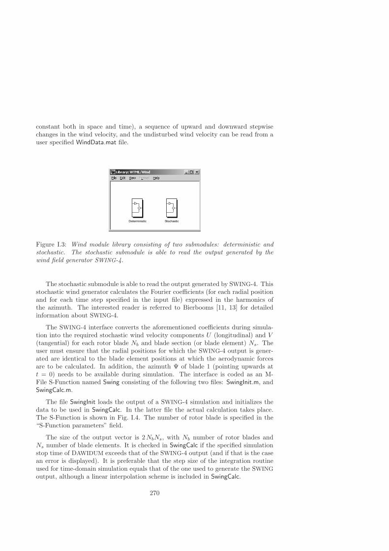
constant both in space and time), a sequence of upward and downward stepwisechanges in the wind velocity, and the undisturbed wind velocity can be read from auser specified WindData.mat file.

Deterministic Stochastic

Figure I.3: Wind module library consisting of two submodules: deterministic andstochastic. The stochastic submodule is able to read the output generated by thewind field generator SWING-4.

The stochastic submodule is able to read the output generated by SWING-4. Thisstochastic wind generator calculates the Fourier coefficients (for each radial positionand for each time step specified in the input file) expressed in the harmonics ofthe azimuth. The interested reader is referred to Bierbooms [11, 13] for detailedinformation about SWING-4.

The SWING-4 interface converts the aforementioned coefficients during simula-tion into the required stochastic wind velocity components U (longitudinal) and V(tangential) for each rotor blade Nb and blade section (or blade element) Ns. Theuser must ensure that the radial positions for which the SWING-4 output is gener-ated are identical to the blade element positions at which the aerodynamic forcesare to be calculated. In addition, the azimuth Ψ of blade 1 (pointing upwards att = 0) needs to be available during simulation. The interface is coded as an M-File S-Function named Swing consisting of the following two files: SwingInit.m, andSwingCalc.m.

The file SwingInit loads the output of a SWING-4 simulation and initializes thedata to be used in SwingCalc. In the latter file the actual calculation takes place.The S-Function is shown in Fig. I.4. The number of rotor blade is specified in the“S-Function parameters” field.

The size of the output vector is 2NbNs, with Nb number of rotor blades andNs number of blade elements. It is checked in SwingCalc if the specified simulationstop time of DAWIDUM exceeds that of the SWING-4 output (and if that is the casean error is displayed). It is preferable that the step size of the integration routineused for time-domain simulation equals that of the one used to generate the SWING

output, although a linear interpolation scheme is included in SwingCalc.

270

Swing1 1

S-Function

Psi [U,V]

Figure I.4: SWING-4 interface in DAWIDUM. Input: Ψ, and outputs: U = [U1(1 :Ns), · · · , UNb

(1 : Ns)] and V = [V1(1 : Ns), · · · , VNb(1 : Ns)] for each blade element

Ns and rotor blade Nb.

I.2.2 Aerodynamic module library

The aerodynamic module is coded as an M-File S-Function named BEM. The S-Function is shown in Fig. I.5 and is built up out of the following two files: AeroInit.m,and AeroCalc.m. The file AeroInit provides an initial guess for both the axial andtangential induction factor, and loads the specified turbulent wake state model. Thismodel is specified in the “S-Function parameters” field. In AeroCalc.m deterministiceffects as wind shear, tower shadow and the ten-minute average wind speed at hubheight are added to the zero-mean stochastic components of SWING-4 before theaerodynamic forces are computed.

Aero

1

1

S-Function

[Vpb,Vtb]

[Fp,Ft]

2

[U,V]

Figure I.5: Aerodynamic module in DAWIDUM. Inputs: [Vpb, Vtb]: blade elementvelocities x, and [U, V ]: SWING-4 output. Outputs: [Fp, Ft] = [Fp,1(1 : Ns) Ft,1(1 :Ns) · · ·Fp,Nb

(1 : Ns) Ft,Nb(1 : Ns)] the aerodynamic forces Faero with Ns the number

of blade elements and Nb the number of rotor blades).

271

I.2.3 Mechanical module library

The mechanical module library contains four submodules describing the structuraldynamics at different level of complexity: Rotor blade, Rotor (3-bladed), Tower (plusfoundation), and Wind turbine (3-bladed) (see Fig. I.6). These modules form thebasis of all different developed (and those to be developed) mechanical models of(flexible) wind turbines. All submodules can be opened by double-clicking, andeach submodule contains several models. The model complexity ranges from rigidmodels that have no effect on the system dynamics to flexible models consisting ofa collection of superelements. The selection of number of superelements depends onthe stiffness of the wind turbine under investigation. The library can be modifiedby dragging new modules or models onto it and saving the resulting system.

Rotor blade Rotor(3-bladed)

Tower

(plus foundation)

Wind turbine

(3-bladed)

Figure I.6: Mechanical module library.

Automated structural modeling procedure: performance

The performance of the automated structural modeling procedure implemented inDAWIDUM can be best illustrated by considering the following two situations:

• Create a new structural model from scratch;

• Modify an existing structural model from the mechanical module library. Inthis case we have to make a distinction between:

– Model configuration and/or complexity changes;

– Parameter changes.

Obviously, to create a new wind turbine model from scratch will be more time-consuming than changing the model configuration (e.g. two or three rotor blades),model complexity (i.e. number of degrees of freedom) or adapting some modelparameters (e.g. replacing the rotor blades by another type). The latter change re-quires only a few minutes, while changing the model configuration and/or complexitywill take a few hours. The time to develop a new model from scratch will range froma couple of hours to a few days depending on the wind turbine configuration underinvestigation.

272

To emphasize that the time needed to generate the equations of motion is neg-ligible with respect to the time to make the aforementioned changes, consider theCPU times required to generate the equation of motion of several DAWIDUM modelslisted in Table I.1. These timings demonstrate that the formulation of one set ofequations (even for the most complex structural models) takes only a few seconds.

Timing comparisons

DAWIDUM model CPU time Complexity

Beam1sd 0.10 s 2Beam3sd 1.25 s 6Beam6sd 1.57 s 12Beam9sd 1.90 s 18SDLW1 2.38 s 20SDLW2 3.77 s 36SDLW3 5.13 s 52

Table I.1: Overview of the CPU time used to generate the equations of motion ofseveral DAWIDUM models on a PC with a 700 MHz Pentium II processor runningWindows-2K with 384 MB RAM. The total number of degrees of freedom (includingfictitious ones) has been used as a measure of complexity.

Rotor blade

The equations implemented in BladePM to compute the centroidal mass momentsof inertia, and center of gravity of all rigid bodies within each superelement willnow be presented. Recall that the mass as well as the flexural rigidity in the twoprincipal bending directions need to be supplied by either the blade designer or theblade manufacturer. The center of gravity of each rigid body with respect to itsbase is determined as follows:

Cg =Lrb∑r=0

m(r) · (R(r) −R(0))/Mrb

with m(r) the mass as function of the local radius r, and Mrb the mass of the rigidbody under consideration which is, in turn, defined as:

Mrb =Lrb∑r=0

m(r)

Subsequently, the centroidal mass moment of inertia is determined as

Jx =Lrb∑r=0

m(r) · (R(r) −R(0)) − Cg2

273

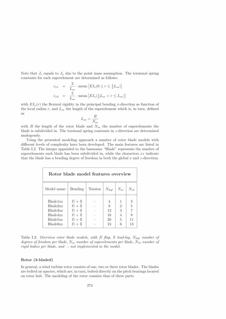
Note that Jz equals to Jx due to the point mass assumption. The torsional springconstants for each superelement are determined as follows:

cx1 =2Lse

· mean[EIx(0 ≤ r ≤ 1

2Lse)]

cx3 =2Lse

· mean[EIx( 1

2Lse < r ≤ Lse)]

with EIx(r) the flexural rigidity in the principal bending x-direction as function ofthe local radius r, and Lse the length of the superelement which is, in turn, definedas

Lse =R

Nse

with R the length of the rotor blade and Nse the number of superelements theblade is subdivided in. The torsional spring constants in z-direction are determinedanalogously.

Using the presented modeling approach a number of rotor blade models withdifferent levels of complexity have been developed. The main features are listed inTable I.2. The integer appended to the basename “Blade” represents the number ofsuperelements each blade has been subdivided in, while the characters xz indicatethat the blade has a bending degree of freedom in both the global x and z-direction.

Rotor blade model features overview

Model name Bending Torsion Ndof Nse Nrb

Blade1xz fl + ll – 4 1 3Blade2xz fl + ll – 8 2 5Blade3xz fl + ll – 12 3 7Blade4xz fl + ll – 16 4 9Blade5xz fl + ll – 20 5 11Blade6xz fl + ll – 24 6 13

Table I.2: Overview rotor blade models, with fl flap, ll lead-lag, Ndof number ofdegrees of freedom per blade, Nse number of superelements per blade, Nrb number ofrigid bodies per blade, and –: not implemented in the model.

Rotor (3-bladed)

In general, a wind turbine rotor consists of one, two or three rotor blades. The bladesare bolted on spacers, which are, in turn, bolted directly on the pitch bearings locatedon rotor hub. The modeling of the rotor consists thus of three parts

274

• Rotor blade

• Spacer

• Rotor hub

The main features of the different developed DAWIDUM rotor models are listedin Table I.3. The integer appended to the basename “Rotor” represents the numberof superelements each blade has been subdivided in, while the p indicates that eachblade has a pitch degree of freedom. The rigid rotor model, i.e. Rotor0p, has beenspecially added for checking out the aerodynamics.

Wind turbine rotor model features overview

Model name Nb Pitching Bending Torsion Ndof Nse Nrb

Rotor0p 3 • – – 0 0 1Rotor1p 3 • f l + ll – 12 1 3Rotor2p 3 • f l + ll – 24 2 5Rotor3p 3 • f l + ll – 36 3 7Rotor4p 3 • f l + ll – 48 4 9Rotor5p 3 • f l + ll – 60 5 11

Table I.3: Overview rotor models, with Nb number of blades, fl flap, ll lead-lag,Ndof total number of degrees of freedom (exclusive pitch, and azimuth), Nse numberof superelements per blade, Nrb number of rigid bodies per blade, –: not implementedin the module, and •: implemented in the model.

Tower (plus foundation)

The equations implemented in TowerPM to compute the mass, inertia (mass mo-ments as well as area moments), and center of gravity of the tapered, hollow towersections are derived given below. The torsional spring constants for each superele-ment are determined as follows:

cx1T =2Et

Lse· mean

[Ix(0 ≤ h ≤ 1

2Lse)]

cx3T =2Et

Lse· mean

[Ix( 1

2Lse < h ≤ Lse)]

with Et the modulus of elasticity, Ix(h) the area moment of inertia as function ofthe local tower height h, and Lse the length of the superelement which is, in turn,

275

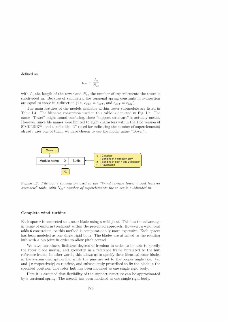
defined as

Lse =Lt

Nse

with Lt the length of the tower and Nse the number of superelements the tower issubdivided in. Because of symmetry, the torsional spring constants in x-directionare equal to those in z-direction (i.e. cx1T = cz1T , and cx3T = cz3T ).

The main features of the models available within tower submodule are listed inTable I.4. The filename convention used in this table is depicted in Fig. I.7. Thename “Tower” might sound confusing, since “support structure” is actually meant.However, since file names were limited to eight characters within the 1.3c version ofSIMULINK R©, and a suffix like “1” (used for indicating the number of superelements)already uses one of them, we have chosen to use the model name “Tower”.

Figure I.7: File name convention used in the “Wind turbine tower model featuresoverview” table, with Nse: number of superelements the tower is subdivided in.

Complete wind turbine

Each spacer is connected to a rotor blade using a weld joint. This has the advantagein terms of uniform treatment within the presented approach. However, a weld jointadds 6 constraints, so this method is computationally more expensive. Each spacerhas been modeled as one single rigid body. The blades are attached to the rotatinghub with a pin joint in order to allow pitch control.

We have introduced fictitious degrees of freedom in order to be able to specifythe rotor blade inertia, and geometry in a reference frame unrelated to the hubreference frame. In other words, this allows us to specify three identical rotor bladesin the system description file, while the pins are set to the proper angle (i.e. 2

3π,and 4

3π respectively) at runtime, and subsequently prescribed to fix the blade in thespecified position. The rotor hub has been modeled as one single rigid body.

Here it is assumed that flexibility of the support structure can be approximatedby a torsional spring. The nacelle has been modeled as one single rigid body.

276

Wind turbine tower model features overview

Model name Bending Torsion Ndof Nse Nrb Foundation

Tower0c x – 1 0 1 –Tower0 x – 1 0 1 –Tower1 x – 2 1 4 –Tower2 x – 4 2 6 –Tower3 x – 6 3 8 –Tower4 x – 8 4 10 –Tower5 x – 10 5 12 –Tower6 x – 12 6 14 –Tower7 x – 14 7 16 –Tower8 x – 16 8 18 –Tower9 x – 18 9 20 –Tower1z x + z – 4 1 4 –Tower2z x + z – 8 2 6 –Tower3z x + z – 12 3 8 –Tower4z x + z – 16 4 10 –Tower5z x + z – 20 5 12 –Tower1f x – 3 1 4 •Tower2f x – 5 2 6 •Tower3f x – 7 3 8 •Tower4f x – 9 4 10 •Tower5f x – 11 5 12 •Tower1zf x + z – 6 1 4 •Tower2zf x + z – 10 2 6 •Tower3zf x + z – 14 3 8 •Tower4zf x + z – 18 4 10 •Tower5zf x + z – 22 5 12 •

Table I.4: Overview tower models, with Ndof number of degrees of freedom, Nse

number of superelements, Nrb number of rigid bodies (including nacelle), –: notimplemented in the module, and •: implemented in the model.

277

I.2.4 Electrical module library

The electrical module library contains two modules, i.e. Elec0, and Elec2, describingthe dynamics of the electromagnetic part of a synchronous generator plus AC-DC-AC

conversion system at different levels of complexity.

Elec0 module

The Elec0 module contains the simplest model. It is assumed that vector control hasbeen successfully applied to the synchronous generator in question, implying thatthe synchronous generator can be viewed as an instantaneous torque source. Sucha controlled generator can be modeled as a first order system with a time constantτTem

derived from the torque response time. The time constant comprises thus boththe power converter and the electromagnetic dynamics of a synchronous generator.The value of the constant is dependent on the switching frequency of the converterand the sampling rate of the torque controller. For example, the torque responsetime of the controlled Elec2 module can be used to derive the time constant τTem

required for simulation of Elec0.

Elec2 module

The Elec2 module contains the most complex generator model in the library. Theelectromagnetic part contains the voltage and flux equations of the synchronousgenerator as described in Section 3.5. This model has been identified, verified andvalidated in Section 4.3 using experimental data acquired from the Lagerwey LW-50/750 synchronous generator. The block diagram of this module is depicted inFig. 3.26 on page 100.

Main features overview

The main features of the two modules are listed in Table I.5. The Elec2 module ismost-suited for designing a frequency converter controller on the basis of a validatedsynchronous generator model, while the Elec0 module is most suited for time-domainwind turbine simulations.

Electrical modules features overview

Time-domain Frequency converterModule name Ordersimulation control design

Elec0 1 ++ −Elec2 ≥ 8† − ++

Table I.5: Overview electrical modules, with †: depends on synchronous generatorunder investigation, ++ suited, − not suited.

278

Bibliography

[1] ABB Reinosa, S.A. Dpto. de Calidad, Ensayos Electricos, Test recordLW50/750, 810 KVA, 690 V, 27 R/min. Generator No. 51210-001, Reinosa,4 Agosto de 1998.

[2] M.B. Anderson, “A vortex-wake analysis of a horizontal axis wind turbineand a comparison with modified blade element theory.” In Proceedings of 3 rd

International Symposium on Wind Energy Systems, Copenhagen, BHRA FluidEngineering, pp. 357–374, 1980.

[3] P.M. Anderson, and A.A. Fouad, Power System Control and Stability. TheIowa State University Press, Ames, Iowa, U.S.A., 464p., 1977.

[4] Anon, Adams User’s Guide, Mechanical Dynmics Inc., 3055 Plymouth Rd.,Ann Arbor, Michigan, 1987.

[5] K.J. Astrom, and T. Hagglund, PID Controllers: Theory, Design and Tuning.Instrument Society of America, Research Triangle Parc, NC, USA, 1995.

[6] G.E. van Baars, Validation of flexible wind turbine dynamic models throughopen field identification experiments. PhD. Thesis, Delft University of Tech-nology, Mechanical Engineering Systems and Control group, (to appear).

[7] Y. Bard, Nonlinear Parameter Estimation. Acdemic Press, New York, 341p.,1974.

[8] N.D.P. Barltrop, and A.J. Adams, Dynamics of fixed marine structures.Butterworth-Heinemann Ltd, Linacre House, Jordan Hill, Oxford, Great-Britain, 764p., 1991.

[9] W.A.A.M. Bierbooms, A dynamic model of a flexible rotor - Part 1: Descrip-tion of the mathematical model. Delft University of Technology, Institute forWind Energy, IW 89.034R, 82p., May 1990.

[10] W.A.A.M. Bierbooms, Modellering van Dynamic Stall met behulp van de On-era Methode. Delft University of Technology, Institute for Wind Energy, IW91.044m, 30p., July 1991.

279

[11] W.A.A.M. Bierbooms, Swing4 User Guide. Delft University of Technology,Institute for Wind Energy, IvW-98133 R, 22p., February 1998.

[12] W.A.A.M. Bierbooms, P.M.M. Bongers, and M. Steinbuch, An integrated dy-namic model of a wind turbine. Delft University of Technology, Institute forWind Energy, IW 87.011 R, 73p., May 1987.

[13] W.A.A.M Bierbooms, and J.B. Dragt (Institute for Wind Energy), “SWING 4:A stochastic 3D wind field generator for design calculations.” In Proceedings ofEuropean Union Wind Energy Conference, EUWEC 1996, Goteborg, Sweden,pp. 942–945, May 20–24, 1996.

[14] A. Bjorck, and S-E. Thor (FFA, The Aeronautical Institute of Sweden), “Dy-namic stall and 3D effects.” In Proceedings of European Union Wind EnergyConference, EUWEC 1996, Goteborg, Sweden, pp. 683–686, May 20–24, 1996.

[15] J.K. de Boer, FLEXLAST 3.0, Description of an analysis tool for the predic-tion of loads on wind turbines. Stork Product Engineering, Amsterdam, TheNetherlands, SPE report 94-040, September 1993.

[16] W.W. de Boer and M.W. Mortier (KEMA, The Netherlands), “Experimentalresults of optimal output feedback controlled wind turbines of the experimentalwind farm.” In Proceedings of European Wind Energy Conference, EWEC1994, Thessaloniki, Macedonia, Greece, pp. 593–598, October 10–14 1994.

[17] T. Bohlin and S.F. Graebe, “Issues in nonlinear stochastic grey box identifi-cation.” In International Journal of Adaptive Control and Signal Processing.Volume 9, pp. 465–490, 1995.

[18] E.S. Boije, J.C. Balda, R.G. Harley, and R.C. Beck, “Time-domain identi-fication of synchronous machine parameters from standstill tests.”, In IEEETransactions on Energy Conversion, Volume 5, No. 1, pp. 164–175, 1990.

[19] I. Boldea, and S.A. Nasar, Electric drives. CRC Press, Inc., Boca Raton,Florida, 411p., 1999.

[20] P.M.M. Bongers, DUWECS Reference guide V2.0, Delft University WindEnergy Converter Simulation Package. Delft University of Technology, TheNetherlands, DUT-MEMT 26, 1993.

[21] P.M.M. Bongers, Modeling and Identification of Flexible Wind Turbines anda Factorizational Approach to Robust Control. PhD. Thesis, Delft Universityof Technology, Faculty of Mechanical Engineering and Marine Technology,Measurement and Control group, June 1994.

[22] P.M.M. Bongers, G.E. van Baars, Sj. Dijkstra and O.H. Bosgra, Dynamicmodels for wind turbines. Delft University of Technology, Faculty of MechanicalEngineering and Marine Technology, Measurement and Control group, memt-28, 115p., 1993.

280

[23] P.M.M. Bongers, W. Bierbooms, Sj. Dijkstra, and T. van Holten, An integrateddynamic model of a flexible wind turbine. Delft University of Technology, Fac-ulty of Mechanical Engineering and Marine Technology, Measurement andControl group, memt-6, 106p., 1990.

[24] P.M.M. Bongers, Th. van Holten and Sj. Dijkstra, “Control of wind turbinesystems for load reduction.” In Proceedings of Wind Energy: Technology andImplementation, EWEC 1991. Amsterdam, The Netherlands, pp. 68–72, 1991.

[25] I. Bonnet, “Tegenwind voor windenergie.” In Delta, No. 36, 23 November 2000.

[26] B.K. Bose, Power Electronics and Variable Frequency Drives. IEEE Press, 445Hoes Lane, P.O. Box 1331, Piscataway, NJ, 640p., 1997.

[27] B. Bosman (TNO Bouw - Centrum voor Mechanische Constructies), “Trilvor-men aan vleugelprofiel: APX-70”, TNO Bouw Memorandum No. 2000-CMC-M288/BNB, 17p., 11 July 2000.

[28] B. Bosman (TNO Bouw - Centrum voor Mechanische Constructies), “Trilvor-men aan een 29m blad”, TNO Bouw Memorandum No. 2002-CMC-B89/BNB,17p., 12 Maart 2002.

[29] E.A. Bossanyi (Garrad Hassan & Partners), Bladed for Windows - TheoryManual. Garrad Hassan & Partners Limited, Bristol, England, Document No.282/BR/009, Issue No. 3, 54p., June 1997.

[30] E.A. Bossanyi (Garrad Hassan and Partners Ltd.), “Developments in closedloop controller design for wind turbines.” In Proceedings of the 2000AIAA/ASME Wind Energy Symposium, Reno, NV, pp. 64–74, January 10-13, 2000.

[31] A. Boxmeer, “Niemand wil een windmolen.” In Intermediair, No. 31, pp. 27–29, 5 August 1999.

[32] A.J. Brand, H. Snel (Netherlands Energy Research Foundation ECN), G.E.van Baars, P.M.M. Bongers (Delft University of Technology), N.O.T. Hansenand G.A.M. van Kuik (Stork Product Engineering), The Dutch contributionto the IEA UNIWEX project. ECN-C-94-075, 61p., September 1994.

[33] BTM Consults ApS, Ten Percent of the World’s Electricity Consumption fromWind Energy! - Is that target achievable? Main report for the Forum forEnergy & Development (FED), BTM Consults ApS, I.C. Christensens Alle 1,DK-6950 Rinkøbing, Denmark, 55p., October 1998.

[34] BTM Consult ApS (www.btm.dk), World Market Update 2001 - Forecast 2002-2006. I.C. Christenses Alle 1, Rinkøbing, Denmark, 66p., March 2002.

[35] J.L. Buchanan, and P.R. Turner, Numerical methods and analysis. Interna-tional series in pure and applied mathematics, McGraw-Hill, New York, 751p., 1992.

281

[36] I.K. Buerings and L.L. Freris, “Control policies for wind energy conversionsystems.” In Proceedings of the IEEE Conference on Control Applications.Volume 128, 1981.

[37] T. Burton, D. Sharpe, N. Jenkins, and E. Bossanyi, Wind Energy Handbook,John Wiley & Sons, Ltd, Baffins Lane, Chichester, West Sussex PO19 1UD,England, 617p., 2001.

[38] T.R. Camp, E.A. Bossanyi, and D.C. Quarton (Garrad Hassanand Partners Limited), “Design loads for offshore wind turbines.”http://www.energyweb.net/articles/gh_design_loads.html,4p, 1999.

[39] R. Cardenas-Dobson (Universidad de Magallanes, Punta Arenas Chile), andG.M. Asher (University of Nottingham, Electrical Engineering Department,United Kindom), “Power Limitation in Variable Speed Wind Turbines usingPitchh Control and a Mechanical Torque Observer.” In Wind Engineering.Volume 20, No. 6, pp. 363–387, 1996.

[40] T.G. Carne, J.P. Lauffer, A.J. Gomez, and H. Benjannet (Sandia NationalLaboratories), Modal Testing the EOLE. Sandia Report SAND87-1506, 24p.,April 1988.

[41] P. Caselitz, W. Kleinkauf, T. Kruger, J. Petschenka (Institut fur Solare En-ergieversorgungstechnik e. V.), and K. Storzel (Fraunhofer-Institut fur Betreib-sfestigkeit), “Load reduction by multivariable control of wind energy conver-tors - simulations and experiments.” In Proceedings of European Union WindEnergy Conference, EUWEC 1996, Goteborg, Sweden, pp. 821–824, May 20–24, 1996.

[42] P. Caselitz, W. Kleinkauf, T. Kruger, J. Petschenka, M. Reichardt (Institut furSolare Energieversorgungstechnik e. V.), and K. Storzel (Fraunhofer-Institutfur Betreibsfestigkeit), “Reduction of fatigue loads on wind energy conver-tors by advanced control methods.” In Proceedings of European Wind EnergyConference, EWEC 1997, Dublin, Ireland, pp. 555–558, October 6–9 1997.

[43] S.K. Chakrabarti, Hydrodynamics of Offshore structures. WIT Press, Compu-tations Mechanical Publications, 440p., 1999.

[44] S.J. Chapman, Electric Machinery Fundamentals. Schaum’s Outline Series inElectronics & Electrical Engineering, McGraw-Hill, Inc., New York, 716p.,1991.

[45] B.W. Char, K.O. Geddes, G.H. Gonnet, B.L. Leong, M.B. Monagan, and S.M.Watt, Maple V Library Reference Manual. Springer-Verlag, 698p., 1992.

[46] G. Chavent, “Identifiability of parameters in output least square formulation.”In E. Walter (editor), Identifiability of parametric models, Pergamon Press, pp.67–74, 1987.

282

[47] P.J. Cloos (Twaron Products V.o.F.), personal communication, November 3,1998.

[48] T. Christensen, J. Pedersen, L.B. Plougmand, S. Mogensen, H. Sterndorf,“Flex5 for offshore environments.” In Proceedings of 2001 European Wind En-ergy Conference and Exhibition, Bella Center, Copenhagen, Denmark July 2–6,2001.

[49] T.H. Cockerill, R. Harrison, M. Kuhn, and G.J.W. van Bussel, Comparison ofCost of Offshore Wind Energy at European Sites, Opti-OWECS Final Report,Volume 3, ISBN 90-76468-04-4, 1998.

[50] J.R. Connell (Pacific Northwest Laboratory, Richland, Washington), “Aprimer of turbulence at the wind turbine rotor.” In Windpower 1985, SanFransisco, California, USA, pp. 57–66, 1985.

[51] A. Dadone, and L. Dambrosio, “Estimator based adaptive fuzzy logic con-trol technique for a wind turbine-generator system.” In Energy Conversion &Management, Volume 44, pp. 135–153, 2002.

[52] J. d’Alembert, Traite de Dynamique, Paris, 1743.

[53] dSPACE R©: http://www.dspace.de/

[54] T.F. Edgar, and D.M. Himmelblau, Optimization of chemical processes.McGraw-Hill International Editions, Chemical Engineering Sciences, Singa-pore, 652p., 1989.

[55] D.M. Eggleston and F.S. Stoddard, Wind turbine engineering design. VanNostrand Reinhold, New York, USA, 352p., 1987.

[56] A.S. Elliott (Mechanical Dynamics, Inc., Ann Arbor, Michigan), andA.D. Wright (National Renewable Energy Department, Golden, Collerado),ADAMS/WT 1.0 User’s Guide and Reference Manual. Version 1.0, February1994.

[57] A.S. Elliott (Mechanical Dynamics, Inc., Ann Arbor, Michigan), andA.D. Wright (National Renewable Energy Department, Golden, Collerado),ADAMS/WT 2.0 User’s Guide. Version 2.0, December 1998.

[58] Energy Information Administration (EIA), International Energy Annual 1999,DOE/EIA-0219(99), Washington, DC, January 2001.

[59] L. Euler, “Nova methods motum corporum rigidarum determinandi.” In NoviCommentarii Academiæ Scientiarum Petropolitanæ, 20, pp. 208–238, 1776.

[60] Wind Energy - The Facts, European Commission, Directorate-General for En-ergy, 1999.

283

[61] L.J. Fingersh, and P.W. Carlin (National Renewable Energy Laboratory,Golden, Colorado), “Results from the NREL variable-speed test bed.” In Pro-ceedings of the 1998 ASME Wind Energy Symposium Technical Papers Pre-sented at the 36th AIAA Aerospace Sciences Meeting and Exhibit, Reno, NV,pp. 233–237, January 12-15, 1998.

[62] P. Fisette, and J.C. Samin (Department of Mechanical Engineering, Universitecatholique de Louvain, Belgium), “The modelling of complex mechanical sys-tems in the Matlab/Simulink environment.” In Proceedings 1st Benelux MatlabUsers Conference, Amsterdam, The Netherlands, Chapter 4 pp. 1–11, October27–28, 1997.

[63] A.E. Fitzgerald, C. Kingsley Jr., and S.D. Umans, Electric Machinery.MacGraw-Hill International (UK) Limited, 599p., 1992.

[64] R. Fletcher, Practical Methods of Optimization. John Wiley & Sons, BaffinsLane, Chichester, West Sussex PO19 1UD, England, 436p., 1987.

[65] L.L. Freris, Wind energy conversion systems. Prentice Hall International(U.K.) Ltd, University Press, Cambridge, 388 p., 1990.

[66] L.N. Freeman, and R.E. Wilson (Department of Mechanical Engineering, Ore-gon State University, Corvallis), “The FAST code.” In Proceedings of the 28 th

IEA Meeting of Experts “State of the Art of Aerolelastic Codes for Wind Tur-bine Calculations”, Technical University of Denmark, Lyngby, pp. 37-56, 11–12April 1996.

[67] P.P. Friedmann (Mechanics and Structures Department, University of Califor-nia), “aero-elastic Modelling of Large Wind Turbines.” In Journal of AmericanHelicopter Society, Volume 21, No. 4, pp. 17–27, October 1976.

[68] R.E. Froude, “On the part played in propulsion by differences of fluid pres-sure.” In Transactions of the Institute of Naval Architects, Volume 30, p. 390,1889.

[69] H. Ganander (Teknikgruppen AB, Sollentuna, Sweden), “The Vidyn story.” InProceedings of the 28 th IEA Meeting of Experts “State of the Art of Aerolelas-tic Codes for Wind Turbine Calculations”, Technical University of Denmark,Lyngby, pp. 77-90, 11–12 April 1996.

[70] H. Ganander, and B. Olsson (Teknikgruppen AB), VIDYN - Time simulationprogram for wind turbines. Version 6, 69p., 14 December 1994.

[71] G.H. Gaonkar and D.A. Peters, “Effectiveness of Current Dynamic-InflowModels in Hover and Forward Flight.” In Journal of the American HelicopterSociety, Volume 31, No. 2, pp. 47–57, April 1986.

[72] G.H. Gaonkar and D.A. Peters, “Review of Dynamic Inflow Modeling for Ro-torcraft Flight Dynamics.” In Vertica, Volume 12, No. 3, pp. 213–242, 1988.

284

[73] A.D. Garrad, “Dynamics of wind turbines.” In IEEE Proceedings, Volume 130,No. 9, pp. 523–530, December 1983.

[74] Bladed for Windows - A Design Tool for Wind Turbine Performance and Load-ing (Offshore Upgrade), http://www.garradhassan.com/bladed/index.htm,2001.

[75] J. Geldermans, “Nut windmolens is te verwaarlozen.”, In Alkmaarse Courant,30 October 2000.

[76] J.M. Gere (Stanford University), and S.P. Timoshenko (Late of StanfordUniversity), Mechanics of Materials. Van Nostrand Reinhold (International),Hong Kong, 762p., 1987.

[77] Germanischer Lloyd, Rules & Guidelines 2000: IV Non-marine Technology -Regulations for the Certification of (Offshore) Wind Energy Conversion Sys-tems, 1999.

[78] M. Geyler, Advanced Pitch Control for Wind Turbines - Literature surveyand first considerations on the potential of pitch control to reduce structuralvibrations and fatigue loads. Duwind Report 2001.001, 68p., January 2001.

[79] P.E. Gill, W. Murray, and M.H. Wright, Practical Optimization. AcademicPress Inc., London, 401p., 1981.

[80] P. Gipe, Wind energy comes of age. John Wiley & Sons, Inc., United Statesof Ameica, 536p., 1995.

[81] H. Glauert, “Airplane propellors.” In W.F. Durand (editor), AerodynamicTheory, Volume 4, pp. 169–360, Springer, Berlin, 1935.

[82] H. Glauert, The Analysis of Experimental Results in Windmill Brake and Vor-tex Ring States of an Airscrew. Reports and Memoranda, No. 1026, London:Aeronautical Research Committee, 1926.

[83] H. Glauert, The elements of airfoil and airscrew theory (second edition). Cam-bridge University Press, 232p., 1959.

[84] Global Business Environment (PXG), Energy Needs, Choices and Possibilities- Scenarios to 2050, www.shell.com/scenarios, Exploring The Future, ShellInternational Limited, Shell Centre, London SE1 7NA, 60p., 2001.

[85] Global Business Environment (PXG), People and Connections - Global Sce-narios to 2020, Public Summary (www.shell.com/scenarios), Exploring TheFuture, Shell International Limited, Shell Centre, London SE1 7NA, 2002.

[86] K.R. Godfrey, and J.J. DiStefano, III, “Identifiability of model parameters.”In E. Walter (editor), Identifiability of parametric models, Pergamon Press,pp. 1–20, 1987.

285

[87] A. de Goederen, “Windenergie parasiteert op de conventionele centrales.”, InHet Parool, 29 April 2000.

[88] S. Goldstein, “On the Vortex Theory of Screw Propellors”. In Roy. Soc. Proc.(A), 123, p. 440, 1929.

[89] R.E. Gormont, “A mathematical model of unsteady aerodynamics and radialflow for application to helicopter rotors.” Final Report, D210-10492-1, TheBoeing company, Vertol division, Philadelphia, PA, USA, 172p., May 1973.

[90] R.J.A. Gorter, Grey-box Identification of Induction Machines: on-line and off-line approaches. PhD. Thesis, Eindhoven University of Technology, December1997.

[91] A. Grace, Optimization Toolbox, The MathWorks, Inc., 21 Eliot Street, SouthNatick, MA, November 1990.

[92] A. Grauers, Design of Direct-driven Permanent-magnet Generators for WindTurbines. Technical report No. 292, Department of Electric Power Engineering,Chalmers University of Technology, Goteborg, Sweden, 1996.

[93] M.J. Grimble, “Two and a Half Degrees of Freedom LQG Controller and Ap-plication to Wind Turbines.” In Proceedings IEEE transactions on automaticcontrol. Volume 39, No. 1, pp. 122–127, January 1994.

[94] “Haarscheurtjes in windmolens”, In De Telegraaf, 14 October 1999.

[95] M.M. Hand, (National Wind Technology Center, NREL), and M.J. Balas (De-partment of Aerospace Engineering Sciences, University of Colorado at Boul-der), “Systematic approach for PID controller design for pitch-regulated, vari-able speed wind turbines.” In Proceedings of the 1998 ASME Wind EnergySymposium Technical Papers Presented at the 36th AIAA Aerospace SciencesMeeting and Exhibit, Reno, NV, pp. 84–94, January 12-15, 1998.

[96] M.M. Hand, (National Wind Technology Center, NREL), and M.J. Balas (De-partment of Aerospace Engineering Sciences, University of Colorado at Boul-der), “Non-Linear and Linear Model Based Controller Design for VariableSpeed Wind Turbines.” In Proceedings of the 3rd ASME/JSME Joint FluidsEngineering Conference, San Francisco, California, pp. 1–6, July 18-23, 1999.

[97] A.C. Hansen (University of Utah, Salt Lake City, UT), User’s Guide to theYaw Dynamics Computer Program YawDyn. 32p., August 1993.

[98] A.C. Hansen (University of Utah, Salt Lake City, UT), YawDyn / Aerodyn.http://www.nrel.gov/wind/software/yawdyndesc.html, 2p., 1998.

[99] A.C. Hansen (University of Utah, Salt Lake City, UT), Yaw dynamics of hor-izontal axis wind turbines. Final Report, National Renewable Energy Labora-tory, NREL/TP-442-4822, 73p., May 1992.

286

[100] A.C. Hansen (Mechanical Engineering Department, University of Utah) andC.P. Butterfield (National Renewable Energy Laboratory, Golden, Colorado),“Aerodynamics of horizontal-axis wind turbines.” In Annu. Rev. Fluid Me-chanics, Volume 25, pp. 115–149, 1993.

[101] L.H. Hansen, L. Helle, F. Blaabjerg, E. Ritchie, S. Munk-Nielsen, H. Bindner,P. Sørensen and B. Bak-Jensen, Conceptual survey of Generators and PowerElectronics for Wind Turbines. Risø National Laboratory, Roskilde, Denmark,Risø-R-1205(EN), 105p., December 2001.

[102] A.C. Hansen, and D.L. Laino (University of Utah, Salt Lake City, UT), User’sGuide to the Wind Turbine Dynamics Computer Programs YawDyn and Aero-dyn for Adams R© - Version 11.0. 79p., 31 August 1998.

[103] F.D. Harris, F.J. Tarzanin, and F.J. Fisher, “Rotor high speed performance -theory versus test.” In Journal American Helicopter Society, Volume 17, 1972.

[104] S. Henschel, and H.W. Dommel, “Noniterative Synchronous Machine Parame-ter Identification from Frequency Response Tests.”, In IEEE Trans. on PowerSystems, Vol. 14, No. 2, pp. 553–560, 1999.

[105] R.L. Hills, Power from wind - A history of windmill technology. CambridgeUniversity Press, 324p., 1994.

[106] E.N. Hinrichsen (Power Technologies, Inc., Schenectady, New York), “Variablerotor speed for wind turbines objectives and issues.” In Windpower 1985, SanFransisco, California, USA, pp. 164–170, 1985.

[107] M.J. Hoeijmakers (Delft University of Technology), Elektrische omzettingen.Delftse Universitaire Pers, 198p., 18 Januari 1997.

[108] M.J. Hoeijmakers (Delft University of Technology), Personal communication.October 6, 1999.

[109] M.G. Hollars, D.E. Rosenthal, and M.A. Sherman, SD/FAST User’s Manual.Symbolics Dynamics, Inc., Version B.2, September 1994.

[110] R. Hooke, and T.A. Jeeves, “Direct search solution of numerical and statisticalproblems.” In Journal of the Association for Computing Machinery, Volume8, pp. 221-229, 1961.

[111] IEEE Standard 115-1995: IEEE Guide: Test Procedures for Syn-chronous Machines Part I – Acceptance and Performance Testing andPart II – Test Procedures and Parameter Determination for DynamicAnalysis (revisions of IEEE Std 115-1983 and IEEE Std 115A-1987 seehttp://standards.ieee.org/catalog/olis/index.html), Institute of Electrical andElectronics Engineers, Inc. New York, NY, 216p., 1996.

287

[112] International Standard IEC 1400–1, Wind turbine generator systems – Part1: Safety requirements. Bureau Central de la Commission ElectrotechniqueInternationale, 3 rue de la Varambe, Geneve, Suisse, First edition, December1994.

[113] International Energy Agency, Needs for Renewables, A Report on a Workshopof the Renewable Energy Working Party (REWP) of the International EnergyAgency (IEA), Paris, France, October 11, 2000.

[114] International Energy Agency, World Energy Outlook, 1999 Insights: Lookingat Energy Subsidies: Getting the Prices Right. International Energy Agency(IEA), Paris, France, 206 p., 1999.

[115] M.T. Iqbal, A.H. Coonick and L.L. Freris, “Dynamic control for variable speedwind turbines.” In Wind Engineering. Volume 18, No. 1, pp. 1–12, 1994.

[116] A.R. Jacobs, Rapport betreffende de funderingswijze van een LW 45/750 wind-turbine met een 50 m mast. Rapport WTXF - 6091. ABT Adviesburau voorBouwtechniek BV, Arnhemsestraat 358, 6881 NK Velp, 27 p., Oktober 1995.

[117] G.H. James III, T.G. Carne, and J.P. Lauffer (Sandia National Laboratories),The Natural Excitation Technique (NExT) for Modal Parameter ExtractionFrom Operating Wind Turbines. Sandia Report SAND92-1666, 46p., February1993.

[118] W. Johnson, Helicopter Theory. Princeton US, 1089p., 1980.

[119] C.N. Jones (Department of Mechanical Engineering, University of Queensland,Brisbane, Australia), “Blade Element Performance in Horizontal-Axis Wind-Turbine Rotors.” In Wind Engineering, Volume 7, No. 3, pp. 129–137, 1983.

[120] I. de Jong (OJA-Services), and H. Bouwmeester. Toepassing windenergie inNederland. Het meerjarenprogramma windenergie 1996-2000 TWIN-2. Novem,August 1996.

[121] J.B. Jonker, Spacar User manual and System Description. Report TM872,Delft University of Technology, Laboratory for Engineering Mechanics, 1988.

[122] P.A. Joosse, G.D. de Winkel, and C. Lindenburg, Natural vibrations of theAPX70 blade, measurements and calculations. WMC group, Delft Universityof Technology, Report WMC 6-00-25, 17 July 2001.

[123] P.A. Joosse, G.D. de Winkel, and C. Lindenburg, Natural vibrations of theRB51 blade, measurements and calculations. WMC group, Delft University ofTechnology, Report WMC 2002-06, 14 May 2002.

[124] P.A. Joosse, G.D. de Winkel, and C. Lindenburg, Natural vibrations of theRB70 blade, measurements and calculations. WMC group, Delft University ofTechnology, Report WMC 2002-17, 14 May 2002.

288

[125] P.E.B. Jourdain, “Note on an analogue at Gauss’ principle of least con-straints”. In Quarterly Journal on Pure Applied Mathematics, 40, pp. 153–197,1909.

[126] J-N. Juang, Applied System Identification. Hall, Inc. Englewood Cliffs, NewJersey, USA, 394p., 1994.

[127] J.L. Junkins (Editor), Mechanics and Control of Large Flexible Structures.American Institute of Aeronautics and Astronautics, Washington, 705p., 1990.

[128] J.L. Junkins, and Y. Kim, Introduction to Dynamics and Control of FlexibleStructures. American Institute of Aeronautics and Astronautics, Washington,452p., 1993.

[129] T.R. Kane (Stanford University), and D.A. Levinson (Lockheed Martin Mis-siles and Space), Dynamics OnLine: Theory and implementation with AU-TOLEV. OnLine Dynamics, Inc., Sunnyvale, CA, United States of America,354p., 1996.

[130] T.R. Kane (Stanford University), and D.A. Levinson (Lockheed Palo Alto Re-search Laboratory), Dynamics: Theory and Applications. McGraw-Hill Seriesin Mechanical Engineering, McGraw-Hill Book Company, 379p., 1985.

[131] T.R. Kane and D.A. Levinson, “Formulations of Equations of Motion for Com-plex Spacecraft.” In Journal of Guidance and Control, Volume 3, No. 2, pp.99–112, March-April 1980.

[132] N.D. Kelley (National Renewable Energy Laboratory, Golden, Colorado),“Full vector (3-D) inflow simulation in natural and wind farm environ-ments using an expanded version of the SNLWIND (Veers) turbulence code.”http://www.nrel.gov/wind/library.html, 9p., 1997.

[133] S.G. Kelly, Fundamentals of Mechanical Vibrations. McGraw-Hill series in me-chanical engineering, New York, 643p., 1993.

[134] N. Kelley, A. Wright, and R. Osgood (National Wind Technology CenterNREL), “A Progress Report on the Characterization and Modeling of a VeryFlexible Wind Turbine Design.” In Proceedings 1999 ASME Wind Energy Sym-posium AIAA/ASME, Reno, Nevada, pp. 243–252, January 11–14 1999.

[135] L. Kendall, M.J. Balas, Y.J. Lee (Department of Aerospace Engineering Sci-ences, University of Colorado at Boulder), and L.J. Fingersh (Wind TechnologyDivision, NREL, Colorado), “Application of Proportional-Integral and Distur-bance Accomodating Control to Variable Speed Variable Pitch Horizontal AxisWind Turbines.” In Wind Engineering. Volume 21, No. 1, pp. 21–38, 1997.

[136] A. Keyhani, H. Tsai, and T. Leksan, “Maximum likelihood estimation of syn-chronous machine parameters from standstill time response data.”, In IEEETransactions on Energy Conversion, Volume 9, No. 1, pp. 98–114, 1994.

289

[137] KIVI, Resultaten van een debat tussen voor- en tegenstanders van windenergie.Report nummer An963057.R20, 31p., Juni 2002.

[138] T. Knudsen, P. Andersen, and S. Toffner-Clausen (Aalborg university, Insti-tute of Electronic Systems, Department of Control Engineering), “ComparingPI and Robust pitch controllers on a 400 kW wind turbine by full scale tests.”In Proceedings of European Wind Energy Conference, EWEC 1997, Dublin,Ireland, pp. 546–550, October 6–9 1997.

[139] G.A.M. van Kuik, On the limitations of Froude’s actuator disc concept. PhD.Thesis, Eindhoven University of Technology, February 1991.

[140] E. Kreuzer (Editor), Computerized symbolic manipulation in mechanics.Springer Verlag, 262p., 1994.

[141] L. Kristensen, and S. Frandsen, “Model for power spectra of the blade ofa wind turbine measured from the moving frame of reference.” In Journalof Wind Engineering and Industrial Aerodynamics, Volume 10, pp. 249–262,1982.

[142] T. Kruger, Regelungsverfahren fur Windkraftanlagen zur Reduktion der mech-anischen Belastung. PhD. Thesis, Universitat Gesamthochschule Kassel, Ger-many, April 1998.

[143] M. Kuhn (Institute for Wind Energy), Dynamics of an Offshore Wind TurbineDigital Simulation. Delft University of Technology, Institute for Wind Energy,IW 93.068 R, 102p., October 1993.

[144] M. Kuhn (Institute for Wind Energy), Dynamics and Design Optimisation ofOffshore Wind Energy Conversion Systems. PhD. Thesis, Delft University ofTechnology, Institute for Wind Energy, May 2001.

[145] W. Kuik (Stentec), “The wind turbine response program, called FKA-12 ofStentec, the Netherlands.” In Proceedings of the 28 th IEA Meeting of Experts“State of the Art of Aerolelastic Codes for Wind Turbine Calculations”, Tech-nical University of Denmark, Lyngby, pp. 147-160, 11–12 April 1996.

[146] G.A.M. van Kuik, “Are wind turbines growing too fast?” In Proceedings ofEuropean Wind Energy Conference and Exhibition, EWEC 2001, Copenhagen,Denmark, July 2-6 2001.

[147] P. Kundur, Power System Stability and Control, McGraw-Hill, Inc., 1176p.,1994.

[148] J.C. Lagarias, J.A. Reeds, M.H. Wright, and P.E. Wright, “Convergence Prop-erties of the Nelder-Mead Simplex Method in Low Dimensions.” In SIAMJournal on Optimization, Volume 9, No. 1, pp. 112–147, 1998.

[149] J.-L. Lagrange, Mecanique Analytique, L’Academie Royal des Sciences, Paris,1788.

290

[150] T.J. Larsen (Risø), email contact, August 12, 2002.

[151] J.P. Lauffer, and T.C. Carne (National Renewable Energy Laboratory),“Modal testing in the design evaluation of wind turbines.” In Windpower 1985,San Fransisco, California, USA, pp. 323–332, 1985.

[152] J.P. Lauffer, T.G. Carne, T.D. Ashwill (Sandia National Laboratories), ModalTesting in the Design Evaluation of Wind Turbines. Sandia Report SAND87-2461, 25p., April 1988.

[153] L.X. Le, and W.J. Wilson, “Synchronous machine parameter identification: atime-domain approach.”, In IEEE Trans. on Energy Conversion, Vol. 3, No.2, pp. 241–248, 1988.

[154] E. Lee, Self-regulating Wind Machine, British patent No. 615, 3p., 9 December1745.

[155] J.L. van Leeuwen, and D.R.V. van Delft (Stevin Laboratorium, Delft Univer-sity of Technology), Full scale tests on the APX45 rotor blade part I; Bladedata, root fixing and test rig. Stevin report 6-96-8, 13p., 8 September 1997.

[156] J.L. van Leeuwen, and D.R.V. van Delft, Full scale tests on the APX45 rotorblade part II; Natural frequency tests. Stevin report 6-96-9, 6p., 10 September1997.

[157] J.G. Leishman, and T.S. Beddoes (Aerodynamics Department, Westland He-licopters Ltd., Yeovil, Somerset, United Kingdom), “A Semi-Empirical Modelfor Dynamic Stall.” In Journal of American Helicopter Society, Volume 34,No. 2, pp. 3–17, July 1989.

[158] D.J. Leith, and W.E. Leithead (Department of Electronic and Electrical Engi-neering, University of Strathclyde, Glasgow, United Kingdom), “Appropriaterealization of gain-scheduled controllers with application to wind turbine reg-ulation.” In International Journal of Control, Volume 65, No. 2, pp. 223–248,1996.

[159] W. Leonhard, Control of Electrical Drives. Springer-Verlag Berlin Heidelberg,430p., 1996.

[160] C. Lindenburg (Netherlands Energy Research Foundation ECN), Personalcommunication, May 15, 2001.

[161] C. Lindenburg (Netherlands Energy Research Foundation ECN), PHATAS-III User’s Manual - Program for Horizontal Axis wind Turbine Analysis andSimulation - version III. ECN Unit Renewable Energy, P.O. Box 1, Petten,The Netherlands, ECN-C-95-040, 124p., May 1996.

[162] C. Lindenburg (Netherlands Energy Research Foundation ECN), Results of thePHATAS-III development. ECN Unit Renewable Energy, P.O. Box 1, Petten,The Netherlands, 7p., 1996.

291

[163] C. Lindenburg, and T. Hegberg (Netherlands Energy Research FoundationECN), PHATAS-IV User’s Manual - Program for Horizontal Axis wind Tur-bine Analysis and Simulation - version IV. ECN Unit Renewable Energy, P.O.Box 1, Petten, The Netherlands, ECN-C-99-093, 137p., May 2000.

[164] C. Lindenburg, and J.G. Schepers (Netherlands Energy Research FoundationECN), PHATAS-III: Program for horizontal axis wind turbine analysis andsimulation, version III - aero-elastic modeling. ECN-C-96-025, 50p., July 1996.

[165] C. Lindenburg, and J.G. Schepers (Netherlands Energy Research FoundationECN), Status of PHATAS-III Release “MAR-1995” - SUN and DOS version.ECN-C-95-015, 44p., May 1996.

[166] L. Ljung, System Identification - Theory for the User. Prentice-Hall, Engle-wood Cliffs, New Jersey, 519p., 1987.

[167] L. Ljung, and T. Glad, “On Global Identifiability for Arbitrary ModelParametrizations.” In Automatica, Volume 30, No. 2, pp. 265–276, 1994.

[168] R.P. Luijendijk (Stentec), TWISTER - Dynamic Response Program for Hori-zontal Axis Wind Turbines. Raadgevend Ingenieursbureau Stentec B.V., Heeg,The Netherlands, R6.24/01.05.97, 15p., 12 May 1997.

[169] J.M. Maciejowski, Multivariable feedback design. Addison-Wesley PublishingCompany, Great Britain, 424p., 1991.

[170] N.M.M. Maia, J.M.M. Silva, J. He, N.A.J. Lieven, R.M. Lin, G.W. Skingle,W-M. To, and A.P.V. Urgueira, Theoretical and Experimental Modal Analysis.Research Studies Press Ltd., Taunton, Somerset, England, 468p., 1997.

[171] D.J. Malcolm, “Modal response of 3-bladed wind turbines.” In Proceedingsof the 2002 AIAA/ASME Wind Energy Symposium, Reno, NV, pp. 246–255,January 14-17, 2002.

[172] D. Manor, A. Croxson, and C. Carpmael, European wind-turbine manufac-tures, Credit Suisse First Boston Corporation, 90p., 26 March 2001.

[173] J. Mann (Risø National Laboratory), Models in Micrometeorology. Risø Na-tional Laboratory, Roskilde, Denmark, Risø-R-727(EN), 127p., March 1994.

[174] J. Mann (Risø National Laboratory), Wind Field Simulation. Risø NationalLaboratory, Roskilde, Denmark, 31p., 28 November 1997.

[175] B.A.H. Marrant, Th. van Holten, and G.A.M. van Kuik, Smart Dynamic RotorControl of Large Offshore Wind Turbines. Duwind Report 2002.012, 43p., May2002.

[176] MARC Analysis Research Corporation, Online Documentation: Mentat 3.1-MARC K7.1, 1997.

292

[177] J. Mathews, Guide to accelerometer installation, Endevo Technical Paper TP319, Endevco Corporation, 30700 Racho Viejo Road, San Juan Capistrano,CA 92675, USA, 4p., 2001.

[178] J. Mathews, Guide to adhesively mounting accelerometers, Endevo TechnicalPaper TP 312, Endevco Corporation, 30700 Racho Viejo Road, San JuanCapistrano, CA 92675, USA, 10p., 2001.

[179] S.E. Mattsson, Modelling and Control of Large Horizontal Axis Wind PowerPlants. PhD. Thesis, Department of Automatic Control, Lund Institute ofTechnology, 176 p., 1984.

[180] R.M. Mayer, Design of Composite Structures Against Fatigue - Applications toWind Turbine Blades, Mechanical Engineering Publications Limited, Suffolk,United Kingdom, 246p., 1996.

[181] K.I.M. McKinnon, “Convergence of the Nelder-Mead simplex method to anonstationary point.” In SIAM Journal on Optimization, Volume 9, No. 1,pp. 148–158, 1998.

[182] Ministerie van Economische Zaken, Derde Energienota, 1995.

[183] Ministerie van Economische Zaken, http://www.ez.nl/groeneenergie/html/,January 2002.

[184] Ministerie van Economische Zaken, Partiele herziening Tweede Structu-urschema Elektriciteitsvoorziening (Locatiekeuze Demonstratieproject NearShore Windpark) - Deel 3 Kabinetsstandpunt. Tweede Kamer, vergaderjaar2000-2001, 27 041, Sdu Uitgevers, ’s-Gravenhage nr.4, 41p., 2001.

[185] S.H. Minnich, “Small signals, large signals, and saturation in generator mod-els.” In IEEE Transactions on Energy Conversion, Volume EC-1, No. 1, pp.95–103, March 1986.

[186] D-P. Molenaar, Control design: a way of reducing fatigue loads on a wind tur-bine? - NedFlex: a flexible, variable rotational speed wind turbine. MechanicalEngineering, Systems and Control Group, Delft University of Technology, TheNetherlands, TUD-WBMR-S-746, November 1995.

[187] D-P. Molenaar, DAWIDUM User’s Guide, Version 1, Mechanical Engineering,Systems and Control Group, Delft University of Technology, The Netherlands,TUD-WBMR-N-552, December 2000.

[188] D-P. Molenaar, Modeling and control of the NedFlex turbine - NedFlex: a flex-ible, variable rotational speed wind turbine. Mechanical Engineering, Systemsand Control Group, Delft University of Technology, The Netherlands, TUD-WBMR-A-746, August 1996.

293

[189] D-P. Molenaar, Modeling the structural dynamics of the Lagerwey LW-50/750turbine. Mechanical Engineering, Systems and Control Group, Delft Universityof Technology, The Netherlands, Report N-522, October 1998.

[190] D-P. Molenaar, State-of-the-art of wind turbine design codes. Mechanical En-gineering, Systems and Control Group, Delft University of Technology, TheNetherlands, Report N-523, March 1999.

[191] D-P. Molenaar, Validation of the structural model of the Lagerwey LW-50/750turbine using modal analyis. Mechanical Engineering, Systems and ControlGroup, Delft University of Technology, The Netherlands, Report N-531, March2001.

[192] B. Montgomerie (Netherlands Energy Research Foundation ECN), Dynamicstall model called “Simple”, ECN-C-95-060, 48p., January 1996.

[193] B. Montgomerie, and A. Zdunek (FFA The Aeronautical Research Institute ofSweden), “Dynamic response in horizontal-axis wind turbines including insta-tionairy aerodynamic effects in the stream tube.” In Proceedings of EuropeanCommunity Wind Energy Conference 1984, Hamburg, Germany, pp. 259–264,October 22–26 1984.

[194] J.J. More, and S.J. Wright, Optimization Software Guide. Society for IndustrialApplied Mathematics (SIAM), Philadelphia, 154p., 1993.

[195] D.J. Murray-Smith, “Enhanced environments for the development and valida-tion of dynamic system models”, In Mathematics and Computers in Simula-tion, Volume 39, Issues 5-6, pp. 459–464, November 1995.

[196] D.J. Murray-Smith, “Methods for the External Validation of Continuous Sys-tem Simulation Models: A Review.” In Mathematical and Computer Modellingof Dynamical Systems, Volume 4, No. 1, pp. 5–31, 1998.

[197] NAG Foundation Toolbox, Numerical Algorithms Group Ltd., September 1996.

[198] Nederlandse voornorm, NVN 11400-0, Wind turbines - Part 0: Criteria fortype-certification - technical criteria, Issue April 1999.

[199] J.A. Nelder, and R. Mead, “A simplex method for function minimization.” InComputer Journal, Volume 7, pp. 308–313, 1965.

[200] I. Newton, Philosophiæ Naturalis Principia Mathematica. Jussu SocietatisRegiæ ac Typis Josephi Streater, London, 1687.

[201] P.E. Nielan (Stanford University and Sandia National Laboratories), andT.R. Kane (Stanford University), “Symbolic Generation of Efficient Simu-lation/Control Routines for Multibody Systems.” In G. Bianchi, and W.Schiehlen (Eds.) - Dynamics of Multibody Systems - IUTAM/IFToMM Sym-posium, Udine, 1985, Springer, Berlin Heidelberg, 1986.

294

[202] D.W. Novotny, and T.A. Lipo, Vector Control and Dynamics of AC Drives.Clarendon Press, Oxford, Great Britain, 440p., 1998.

[203] Offshore Wind Energy Ready to Power a Sustainable Europe. Final ReportConcerted Action on Offshore Wind Energy in Europe, Duwind 2001.006, De-cember 2001.

[204] C. Onwubiko, Introduction to Engineering Design Optimization. Prentice Hall,Upper Saddle River, New Jersey, 312p., 2000.

[205] E. Overaa, S.E. Mattsson, and A. Rantzer (Department of Automatic Control,Lund Institute of Technology, Lund, Sweden), “Robustness analyis of a windpower plant.” In Proceedings of European Control Conference 1997, Brussels,Belgium, 1–4 July 1997.

[206] S. Øye (Technical University of Denmark), “Dynamic stall - simulated as timelag of separation”. In IEA Synposium on the aerodynamics of wind turbines.Great Britain, November, 1990.

[207] S. Øye (Technical University of Denmark), FLEX 4 - Metoder. 10 p., 1998.

[208] S. Øye (Technical University of Denmark), “FLEX 4 - Simulation of WindTurbine Dynamics.” In Proceedings of the 28 th IEA Meeting of Experts “Stateof the Art of Aerolelastic Codes for Wind Turbine Calculations”, TechnicalUniversity of Denmark, Lyngby, pp. 71-76, 11–12 April 1996.

[209] S. Øye (Technical University of Denmark), “Unsteady effects caused by pitchangle changes”. In IEA Synposium - joint action on aerodynamics of windturbines. London, Great Britain, October 15, 1986.

[210] M.J.D. Powell, “An efficient method for finding the minimum of a functionof several variables without calculating derivatives.” In Computer Journal,Volume 7, pp. 155–162, 1964.

[211] R.H. Park, “Two-Reaction Theory of Synchronous Machines, GeneralizedMethod of Analysis.” Part I: In AIEE Transactions, Vol. 48, pp. 716-730,July 1929.

[212] R.H. Park, “Two-Reaction Theory of Synchronous Machines, GeneralizedMethod of Analysis.” Part II: In AIEE Transactions, Vol. 52, pp. 352-355,June 1933.

[213] M. Pasler, Prinzipe der Mechanik, Walter de Gruyter & Co., Berlin, 147p.,1968.

[214] B.M. Pedersen. “State of the Art of aero-elastic Codes for Wind Turbine Calcu-lations - summary”. In Proceedings of the 28 th IEA Meeting of Experts “Stateof the Art of aero-elastic Codes for Wind Turbine Calculations”, TechnicalUniversity of Denmark, Lyngby, pp. 207-208, 11–12 April 1996.

295

[215] J.T. Petersen, “The aero-elastic code HawC - Model and Comparisons.” InProceedings of the 28 th IEA Meeting of Experts “State of the Art of Aerolelas-tic Codes for Wind Turbine Calculations”, Technical University of Denmark,Lyngby, pp. 129-135, 11–12 April 1996.

[216] D. Petot (Onera, Chatillon Cedex), “Modelisation du decrochage dynamiquepar equations differentielles.” In La Recherche Aerospatiale, Annee 1989, No.5 (Septembre-Octobre), pp. 59–72, 1989.

[217] D. Petot, “Progress in semi-empirical prediction of the aerodynamic forces dueto large amplitude oscillations of an airfoil in attached or separated flow.” InNinth European Rotorcraft Forum, Paper No. 12, Stresa, Italy, 1983.

[218] D.M. Pitt (U.S. Army Aviation Research and Development Command, St.Louis), and D.A. Peters (Washington University, St. Louis), “Theoretical pre-diction of dynamic-inflow derivatives”. In Vertica, Volume 5, pp. 21–34, 1981.

[219] H. Polinder, On the losses in high-speed permanent-magnet generator with rec-tifier - with special attention to the effect of a damper cylinder. PhD. Thesis,Delft University of Technology, Faculty of Electrical Engineering, Power Elec-tronics and Electrical Machines department, June 1998.

[220] H. de la Vallee Poussin, D. Grenier, F. Labrique, and J-D. Legat, “Looking intothe implementation of AC motor control on a fixed point processor.” In Pro-ceedings of the IEEE International Electric Machines and Drives ConferenceIEMDC’99, Seattle, Washington USA, pp. 519-521, May 9–12, 1999.

[221] L. Prandtl, Appendix to “Schraubenpropellor mit gerngstein Energieverlust”by A. Betz, Gottinger Nachr., pp. 193–217, 1919.

[222] B.R. Prentice, “Fundamental concepts of synchronous machine reactances.”In AIEE Transactions, Volume 56 (Suppl. 1), pp. 716–720, 1929.

[223] A. Pubanz, “Specifications for the LW-50/750 Back to back convertor - version1.0.” Lagerwey Windturbine B.V., P.O. Box 279, 3770 AG, Barneveld, TheNetherlands, July 1, 1997.

[224] A. Pubanz, “Calculated machine parameters - Lagerwey 50/750 B2 genera-tor” Lagerwey Windturbine B.V., P.O. Box 279, 3770 AG, Barneveld, TheNetherlands, February 28, 2000.

[225] P.C. Putnam, Final Report on the Smith-Putnam Wind Turbine. EngineeringResearch Division, New York University, War Production Board, 1948.

[226] D.C. Quarton (Garrad Hassan & Partners Ltd., Bristol, United Kingdom),“Calculation of Wind Turbine aero-elastic Behaviour - The Garrad HassanApproach.” In Proceedings of the 28 th IEA Meeting of Experts “State of theArt of Aerolelastic Codes for Wind Turbine Calculations”, Technical Univer-sity of Denmark, Lyngby, pp. 3-12, 11–12 April 1996.

296

[227] D.C. Quarton (Garrad Hassan & Partners Ltd.), “The Evolution of WindTurbine Design Analysis - A Twenty Year Progress Review.” In Wind Energy,Volume 1, pp. 5–24, 1998.

[228] D.C. Quarton (Garrad Hassan & Partners Ltd.), F. Rasmussen (Risø NationalLaboratory), C. Nath, and K. Argyriadis (Germanischer Lloyd), “Wind tur-bine design calculations - The state of the art.” In Proceedings of EuropeanUnion Wind Energy Conference, EUWEC 1996, Goteborg, Sweden, pp. 10–15,May 20–24, 1996.

[229] L.W.M.M. Rademakers and A.P.W.M. Curvers, Global verification of the“Handbook wind data for the design of wind turbines”. ECN-C-91-037, June1991.

[230] L.W.M.M. Rademakers and P.A. van der Werff (Netherlands Energy ResearchFoundation ECN, Verification of wind turbine design codes with the “Dutchhandbook wind data for wind turbine design”. ECN-I-92-048, 12p., December1992.

[231] W.J.M. Rankine, “On the mechanical principles of the action of propellors.”In Transactions of the Institute of Naval Architects, Volume 6, p. 13, 1865.

[232] J. Rauh, Ein Beitrag zur Modellierung elastischer Balkensysteme.Fortschritt-Berichte VDI, VDI-Verlag GmbH, Dusseldorf, Reihe 18:Mechanik/Bruchmechanik, Nr. 37, 126p., 1989.

[233] J. Rauh, and W. Schiehlen, “Various approaches for the Modeling of FlexibleRobot Arms.” In Proceedings of the Euromech-Colloquium 219 on Refined Dy-namical Theories of Beams, Plates, and Shells and their Applications, Kassel,1986, Springer-Verlag, Berlin Heidelberg, pp. 420–429, 1987.

[234] K.J. Reckdahl, and P.C. Mitiguy, AUTOLEV 3 Tutorial. OnLine Dynamics,Inc., Sunnyvale, CA, United States of America, 64p., March 12, 1996.

[235] M. Rees (aerodyn Energiesysteme GmbH, Rendsburg, Germany), and A. Vol-lan (Pilatus Flugzeugwerke, Stans, Switzerland), “Garos: an aero-elastic codefor coupled fixed rotating structures.” In Proceedings of the 28 th IEA Meetingof Experts “State of the Art of Aerolelastic Codes for Wind Turbine Calcu-lations”, Technical University of Denmark, Lyngby, pp. 97-104, 11–12 April1996.

[236] V.A. Riziotis, and S. Voutsinas (National Technical University of Athens, Hel-las), “GAST: A General Aerodynamic and Structural Prediction Tool for WindTurbines.” In Proceedings of European Wind Energy Conference, EWEC 1997,Dublin, Ireland, pp. 448–452, October 6–9 1997.

[237] V.A. Riziotis, and S.P. Voutsinas (National Technical University of Athens,Hellas), “Dynamic Stall on Wind Turbine Rotors: Comparative EvaluationStudy of Different Models.” In Proceedings of European Wind Energy Confer-ence, EWEC 1997, Dublin, Ireland, pp. 481–484, October 6–9 1997.

297

[238] S.M. Rock, A.J. Eggers, P.J. Moriarty, and K. Chaney (RANN Incorporated,Palo Alto, CA), “Tradeoffs in Active Control of Aerodynamic Power and Loadson a HAWT Rotor.” In Proceedings of the 2000 AIAA/ASME Wind EnergySymposium, Reno, NV, pp. 75–83, January 10-13, 2000.

[239] R.V. Rodenburg (Institute for Wind Energy, Delft University of Technology),“FOCUS, a design tool for structural optimization of rotor blades.”

[240] R.V. Rodenburg (Institute for Wind Energy, Delft University of Technology),FOCUS 3.0 manual. Manual for the use of FOCUS 3.0, IW 94081R, November1994.

[241] R.V. Rodenburg, C. Biever, and J.K. de Boer, “Design of the APX45/750 rotorblade with the integrated design tool FOCUS.” In Contributions EuropeanUnion Wind Energy Conference, EUWEC 1996, Goteborg, Sweden, IW-96106,pp. 37–40, May 1996.

[242] R.P.J.O.M. van Rooij, and W.A. Timmer, Aerodynamic design of the APX-45and APX-48 rotors. Delft University of Technology, Institute for Wind Energy,IW 97.129 R, 43p., Oktober 1997.

[243] D.E. Rosenthal, and M.A. Sherman (Symbolic Dynamics, Inc., California),“High Performance Multibody Simulations via Symbolic Equation Manipula-tion and Kane’s Method.” In Journal of the Astronautical Sciences, Volume34, No. 3, pp. 223–239, July-September, 1986.

[244] S. Rozendaal, “De Windoorlog.” In Elsevier, pp. 108–111, 7 October 2000.

[245] S.A. de la Salle, D. Reardon, W.E. Leithead, and M.J. Grimble (IndustrialControl Unit, Department of Electronic and Electrical Enginering, Universityof Strathclyde, Scotland, United Kingdom), “Review of wind turbine control.”In International Journal of Control, Volume 52, No. 6, pp. 1295–1310, 1990.

[246] M.S. Sarma, Synchronous Machines - Their Theory, Stability, and ExcitationSystems. Gordon and Breach, Science Publishers, Inc., New York, 582p., 1979.

[247] T. Sarpkaya, and M. Isaacson, Mechanics of Wave Forces on Offshore Struc-tures, Van Nostrand Reynold Company, 651p., 1981.

[248] R.M. Saunders, “Synchronous-machine standstill frequency-response test dataanalysis”, In IEEE Trans. on Energy Conversion, Vol. 6, No. 3, pp. 564–571,1991.

[249] Scadas II User Manual (Version 8906 Rev. 9111), Difa Measuring SystemsB.V., P.O. Box 3132, 4800 DC, Breda, The Netherlands, 1991.

[250] D.B. Schaeter, D.A. Levinson, and T.R. Kane, Autolev user’s manual. OnlineDynamics, Inc. Sunnyvale, CA 94087, United States of America, 1991.

298

[251] J.G. Schepers, H.J. van Grol, and H. Snel (ECN), Kwalificatie rekenpro-gramma’s horizontale as turbines (KRH). Report ECN-89-96, Petten, TheNetherlands, June 1989.

[252] W. Schiehlen (Editor), Multibody Systems Handbook. Springer Verlag, BerlinHeidelberg, 432p., 1990.

[253] W. Schiehlen, Anleitung Programmsystem NEWEUL, Institut B fur Mechanik,Universitat Stuttgart, Pfaffenwaldring 9, 70550, Stuttgart, 79p.

[254] S.C.S. Technical Committee on Model Credibility, “Termininology for modelcredibility.” In Simulation, Volume 32, pp. 103–104, 1979.

[255] SD/FAST Interface. The MathWorks, Inc., 18p., May 1994.

[256] R. Serban, and J.S. Freeman, “Identification and Identifiability of UnknownParameters in Multibody Dynamic Systems.” In Multibody System Dynamics,Volume 5, pp. 335–350, 2001.

[257] A.A. Shabana, “Flexible Multibody Dynamics: Review of Past and RecentDevelopments.” In Multibody System Dynamics, Vol. 1, Issue 2, pp. 189–222,June 1997.

[258] A.A. Shabana, “Substructure synthesis methods for dynamic analysis of multi-body systems.” In Computers and Structures, Vol. 20, No. 4, pp. 737–744,1985.

[259] D.J. Sharpe (CREST, Loughborough University, United Kingdom), “Basicwind turbine aerodynamics.” In Wind Power Technology Course, Centre forRenweable Energy Systems Techmology, Loughborough University, UnitedKingdom, 29 June - 3 July 1998.

[260] Shell International Limited, The Evolution of the World’s Energy Systems,7p., 1996.

[261] D.G. Shepherd, “Wind Power.” In P. Auer - Advances in Energy Systems andTechnology, Volume 1, Academic Press, New York, pp. 2–124, 1978.

[262] Y. Shimizu, H. Imamura, S. Matsamura, T. Maeda (Department of MechanicalEngineering, Mie University, Tsu-shi, Mie-ken, Japan) and G.J.E. van Bussel(Institute for Wind Energy, Delft University of Technology, Stevinweg 1, TheNetherlands), “Power augmentation of horizontal axis wind turbine by Mie(tip) vane: velocity distribution around tip of HAWT blade with and withoutMie (tip) vane.” In Proceedings of the 16th Annual Energy - Sources TechnologyConference and Exhibition. Houston, Texas, United States of America, SolarEnergy Division, SED-Volume 14, pp. 143–148, ASME 1993.

[263] M. Shinozuka, and C.-M. Jan, “Digital Simulation of Random Processes andits Applications.” In Journal of Sound and Vibration, Volume 25, No. 1, pp.111-128, 1972.

299

[264] SIMULINK, Using SIMULINK- version 4.1. The Mathworks Inc., Natick, MA,United States of America, 6 April 2001.

[265] J.D. Smith, Vibration Measurement and Analysis. Butterworths & Co. (Pub-lishers) Ltd., 166p., 1989.

[266] H. Snel (Netherlands Energy Research Foundation ECN), “Heuristic Modellingof Dynamic Stall Characteristics.” In Proceedings of European Wind EnergyConference, EWEC 1997, Dublin, Ireland, pp. 429-433, October 6–9 1997.

[267] H. Snel (Netherlands Energy Research Foundation ECN), “Review of thePresent Status of Rotor Aerodynamics.” In Wind Energy, Volume 1, pp. 46–69,1998.

[268] H. Snel (Netherlands Energy Research Foundation ECN), R. Houwink, J. Boss-chers, W.J. Piers (National Aerospace Laboratory NLR), G.J.W. van Bus-sel, and A. Bruining (Delft University of Technology) “Sectional predictionof 3D-effects for stalled flow on rotating blades and comparison with mea-surements.” In Proceedings of European Community Wind Energy Conference1993, Lubeck-Travemunde, Germany, pp. 395–399, March 8–12 1993.

[269] H. Snel and J.G. Schepers (Netherlands Energy Research Foundation ECN),Engineering models for dynamic inflow phenomena. ECN report ECN-RX-91-064, 9p., June 1991.

[270] H. Snel and J.G. Schepers (Netherlands Energy Research Foundation ECN),“Investigation and Modelling of Dynamic Inflow Effects.” In Proceedings ofEuropean Community Wind Energy Conference 1993, Lubeck-Travemunde,Germany, pp. 371–375, March 8–12 1993.

[271] H. Snel and J.G. Schepers (Netherlands Energy Research Foundation ECN),Joint investigation of dynamic inflow effects and implementation of an engi-neering method. ECN-C-94-107, 326p., April 1995.

[272] H. Snel and J.G. Schepers (Netherlands Energy Research Foundation ECN),Joint investigation of dynamic inflow effects and implementation of an engi-neering method for response calculations. PE-Memo-91-26, 17p., June 1991.

[273] H. Snel and J.G. Schepers (Netherlands Energy Research Foundation ECN),Short description of aerodynamic research in the Joule dynamic inflow projectsand of the results obtained. ECN-R-93-014, 11p., September 1993.

[274] H. Snel, R. Houwink, and J. Bosschers (Netherlands Energy Research Foun-dation ECN), Sectional prediction of lift coefficients on rotating wind turbineblades in stall. ECN-C-93-052, 72p., December 1994.

[275] H. Snel, and C. Lindenburg (Netherlands Energy Research Foundation ECN),PHATAS-II: Program for horizontal axis wind turbine analysis and simulation,version II - aero-elastic modeling. ECN-C-92-027, 73p., May 1992.

300

[276] Y.D. Song, “Control of Wind Turbines Using Memory-Based Method.” InProceedings of the American Control Conference. Philadelphia, Pennsylvania,pp. 1715–1719, June 24–26, 1998.

[277] J.N. Sørensen, and M.O.L. Hansen (Department of Energy Engineering, Tech-nical University of Denmark), “VISCWIND: A European Collaborate Efforton Viscous Effects of Wind Turbine Blades.” In Proceedings of European WindEnergy Conference, EWEC 1997, Dublin, Ireland, pp. 440–443, October 6–91997.

[278] W. Spendley, G.R. Hext, and F.R. Himsworth, “Sequential application of sim-plex designs in optimization and evolutionary operation.” In Technometrics,Volume 4, pp. 441-461, 1962.

[279] D.A. Spera (Editor), Wind turbine technology: fundamental concepts of windturbine engineering. The American Society of Mechanical Engineers (ASME),638p., 1994.

[280] D.A. Spera (Editor), Wind turbine technology: fundamental concepts of windturbine engineering - Chapter 5 - Aerodynamic Behavior of Wind Turbines.The American Society of Mechanical Engineers (ASME), pp. 215–260, 1994.

[281] M. Steinbuch, Dynamic modeling and robust control of a wind energy conver-sion system. PhD. Thesis, Delft University of Technology, Faculty of Mechan-ical Engineering and Marine Technology, Measurement and Control group,November 1989.

[282] F.S. Stoddard (University of Massachusetts), “Momentum theory and flowstates for windmills.” In Wind Technology Journal, Volume 1, No. 1, pp. 3–9,Spring 1977.

[283] K. Stol, Dynamics Modeling and Periodic Control of Horizontal-Axis WindTurbines, PhD. thesis, Department of Aerospace Engineering Sciences, Facultyof the Graduate School of the University of Colorado, 2001.

[284] H.J. Sutherland (Wind Energy Technology, Sandia National Laboratories, Al-buquerque, New Mexico, United States of America), On the Fatigue Analysisof Wind Turbines”. Sandia National Laboratories, SAND99-0089, 133p., June1999.

[285] H.J. Sutherland, and P.S. Veers (Wind Energy Department, Sandia NationalLaboratories), “Fatigue Case Study and Reliability Analyses for Wind Tur-bines.” In 1995 International Solar Energy Conference, ASME/JSME/JSES,7p., 1995.

[286] J. Svensson, Grid-Connected Voltage Source Converter - Control Principlesand Wind Energy Applications. Technical report No. 331, Department of Elec-tric Power Engineering, Chalmers University of Technology, Goteborg, Swe-den, March 1998.

301

[287] System Identification Toolbox User’s Guide. The MathWorks, Inc. August1995.

[288] I. Szabo, Geschichte der mechanischen Prinzipien, Birkhauser, Basel, 1977.

[289] K. Thomsen, F. Rasmussen, S. Øye, and S.M. Petersen (Risø National Labo-ratory, Roskilde, Denmark), “Loads and Dynamics for Stall Regulated WindTurbines.” Risø-R-655(EN), 43p., July 1993.

[290] W.A. Timmer, and R.P.J.O.M. van Rooij, De profielgegevens voor deAerodynamische Tabel Generator. Sectie Windenergie, Faculteit Civiele Tech-niek en Geowetenschappen, Technische Universiteit Delft, rapport WE-011079,30p., November 2001.

[291] O. Touhami, H. Guesbaoui, and C. Iung, “Synchronous Machine ParameterIdentification by a Multitime Scale Technique.” In IEEE Trans. on IndustrialApplications, Volume 30, No. 6, pp. 1600–1608, 1994.

[292] M.A. Townsend (University of Virginia, Charlottesville, Virginia), “Kane’sEquations, Lagrange’s equations, and Virtual work.” In Journal of Guidanceand Control, Volume 15, No. 1, pp. 277–280, January-February 1992.

[293] C.T. Tran and D. Petot, “Semi-empirical model for the dynamic stall of airfoilsin view of the application to the calculation of responses of a helicopter blade inforward flight.” In 6th European Rotorcraft and Powered Lift Aircraft Forum,Paper No. 48, Bristol, England, 1980.

[294] A. Tumageanian, and A. Keyhani, “Identification of synchronous machine lin-ear parameters from standstill step voltage input data.”, In IEEE Trans. onEnergy Conversion, Vol. 10, No. 2, pp. 232–240, June 1995.

[295] P. Valk, “SD/FAST - Matlab 6.0 Interface.” Mechanical Engineering Systemsand Control Group, Delft University of Technology, The Netherlands, 6p., 19July 2001.

[296] P.S. Veers, Three-Dimensional Wind Simulation. Sandia National Laborato-ries, SAND88-0152, March 1988.

[297] D. Veldkamp (NEG Micon), personal communication, May 15, 2001.

[298] A.T. Veltman, and P.P. Souille (Netherlands Energy Research FoundationECN), “Cost-performance of direct drive wind turbine generators.” In Proceed-ings of European Union Wind Energy Conference, EUWEC 1996, Goteborg,Sweden, pp. 410–413, May 20–24, 1996.

[299] B. Visser (Stork Product Engineering), “The aero-elastic code FLEXLAST.”In Proceedings of the 28 th IEA Meeting of Experts “State of the Art of Aerole-lastic Codes for Wind Turbine Calculations”, Technical University of Den-mark, Lyngby, pp. 161-166, 11–12 April 1996.

302

[300] L.A. Viterna, and R.D. Corrigan (NASA Lewis Research Center, Cleveland,Ohio), “Fixed pitch rotor performance of large horizontal axis wind turbines.”Presented at DOE/NASA Workshop on large horizontal axis wind turbines,Cleveland, United States of America, pp. 69–85, 1981.

[301] J.M. Vleeshouwers, Synchronous machine identification by a simple step-response test. PhD. Thesis, Eindhoven University of Technology, April 1998.

[302] S. Voutsinas (National Technical University of Athens, Hellas), personal com-munication, January 29, 1998.

[303] E. Walter, Identifiability of state space models; with applications to transfor-mation systems. Series Lecture notes in biomathematics 46, Springer, Berlin,202 p., 1982.

[304] F.H. Walter, S.L. Morgan, L.R. Parker Jr., and S.N. Deming,Sequential Simplex Optimization. Electronic reprint MultiSimplex AB“www.multisimplex.com”, 404p., June 1999.

[305] W. Weaver, S.P. Timoshenko, and D.H. Young (Stanford University), Vibra-tion problems in engineering. John Wiley & Sons, Inc., New York, 610p., 1990.

[306] B. Wilson (Oregon State University), FAST-AD - An aerodynam-ics and dynamics analysis code for horizontal-axis wind turbines.http://www.nrel.gov/wind/software/fastaddesc.html, 1p., 6 Februari 1998.

[307] R.E. Wilson, P.B.S. Lissaman, and S.N. Walker, Aerodynamic Performance ofWind Turbines. ERDA/NSF/04014-76/1, Washington, DC: U.S. Departmentof Energy, 1976.

[308] R.E. Wilson, and S.N. Walker, Performance Analysis of Horizontal Axis WindTurbines. Corvallis, Oregon: Oregon State University, 1984.

[309] R.E. Wilson, S.N. Walker, and P. Heh (Department of Mechanical Engineer-ing, Oregon State University, Corvallis), “Technical and user’s manual for theFAST-AD advanced dynamics code.” OSU/NREL Report 99-01, 185p., May1999.

[310] Wind farm closes down after blade snaps. In BBB NEWS - news.bbc.co.uk, 23January 2002.

[311] “Windmolens Eemshaven metaalmoe”, In De Telegraaf, 18 September 1996.

[312] Windpower Monthly News Magazine, “Search archives”,http://www.windpower-monthly.com/.

[313] G.D. de Winkel, P.A. Joosse, and D.R.V. van Delft, STABTOOL project.Part: Determination eigenfrequencies of the APX70 rotor blade using FEM(confidential). WMC group, Delft University of Technology, Report WMC 6-01-19, 26 June 2001.

303

[314] D. Winkelaar, “ROWS: Random Ocean Wave Simulator.” ECN-x-xx-xxx, InPreparation.

[315] D. Winkelaar, “SWIFT: Program for the three dimensional wind simulation,Part 1: Model description and program verification.” ECN-R-92-013, Decem-ber 1992.

[316] P.Th.L.M. van Woerkom, “Modified dynamics modelling for maneuvering flex-ible space manipulators.” In Journal of Sound and Vibration, Volume 179, No.5, pp. 777–792, 1995.

[317] L.R. Brown, C. Flavin, H. French, J.N. Abramovitz, S. Dunn, G. Gardner, L.Mastny, A. Mattoon, D. Roodman, P. Sampat, M.O. Sheehan, and L. Starke,State of the world 2001. A Worldwatch Institute report on Progress Toward aSustainable Society, Earthscan Publications Ltd, London, 275p., 2001.

[318] A.D. Wright (National Renewable Energy Laboratory, Golden, Colorado),“aero-elastic code development activities in the United States.” In Proceedingsof the 28 th IEA Meeting of Experts “State of the Art of Aerolelastic Codes forWind Turbine Calculations”, Technical University of Denmark, Lyngby, pp.25-36, 11–12 April 1996.

[319] A.D. wright, N.D. Kelley, and R.M. Osgood (NREL), “Validation of a modelfor a two-bladed flexible rotor system: progress to date.” In Proceedings 1999ASME Wind Energy Symposium AIAA/ASME, Reno, Nevada, pp. 293–307,January 11–14 1999.

[320] A.D. Wright, C.E. Smith, R.W. Thresher, and J.L.C. Wang, “Vibration Modesof Centrifugally Stiffened Beams.” In Journal of Applied Mechanics, Volume49, pp. 197–202, March 1982.

[321] H.E. Wulff, Traditional Crafts of Persia, Their Development, Technology, andInfluence on Eastern and Western Civilization, The MIT Press, Cambridge,Massachusetts, 304p., 1966.

[322] A. Yeznasni, R. Derdelinckx, and Ch. Hirsch, “Influence of dynamic stall in theaerodynamic study of a HAWT.” In Proceedings of Wind Energy: Technologyand Implementation, EWEC 1991. Amsterdam, The Netherlands, pp. 56–60,1991.

304

Definitions

Aerofoil: Shape of a cross-section of a rotor blade.

Angle of attack (α): Angle between the resultant (or relative) wind velocity andthe chord line of a blade section.

Aspect ratio (AR): Ratio of the rotor blade radius R to the average blade chordlength c (large aspect ratio: c/R 1).

Capacity factor: The capacity factor is defined as the wind turbine’s annualelectricity yield (in kWh) divided by the electricity output if the turbine would haveoperated at its rated power output for the entire year (i.e. the installed power times365 days times 24 hours). Reasonable capacity factors range from 0.25 to 0.30, whilea very good capacity factor would be 0.40.

Capital cost: The capital cost include the purchase price, cost of transporting,assembling, and erecting a wind turbine on site, as well as the cost of installing gridlines and connecting the turbine to the grid.

Chord (c): Width of a cross-section of a rotor blade, i.e. local dimension perpen-dicular to the blade radius R.

Coherent gusts: Gusts of wind with dimensions larger than the rotor swept area,see non-coherent gusts.

Control system: Device of which the dynamics interact with the dynamics of aphysical system (e.g. a wind turbine), and so have implications for the obtainedperformance.

Damping: Damping is the dissipation of energy with time or distance.

305

Degrees of freedom: The number of degrees of freedom of a mechanical systemis equal to the minimum number of independent coordinates required to define com-pletely the positions of all parts of the system at any instant of time. In general, itis equal to the number of independent displacements that are possible.

Downwind: Used to indicate that the rotor is placed at the back of the tower asseen from the main wind direction, cf. upwind.

Drive-train: Part of a wind turbine consisting of the rotor shaft, rotor inertia,transmission, and generator.

dSPACE: dSPACE R© is a real-time system for data-acquisition, controller imple-mentation, and hardware-in-the-loop (HIL) simulation.

Dynamic stall: Dynamic stall or stall hysteresis is a dynamic effect which occurson aerofoils if the angle of attack changes more rapidly than the air flow aroundthe blade (or blade element) can adjust to. The result is aerofoil lift and dragcoefficients which depend not only on the instantaneous angle of attack (quasi-steadyaerodynamics assumption), but also on the recent angle of attack history.

Euler-Bernoulli beam: A prismatic beam with length L, cross-section area A =π ·R2, constant flexural rigidity EI, and uniformly distributed mass per unit lengthρ = m/L, where m is the total mass of the beam. It is assumed that both the sheardeformation and rotational inertia of the cross-sections are negligible if comparedwith bending deformation and translational inertia, respectively. This assumptionleads to a good approximation if the beam is very slender (i.e. R L).

External cost: Cost associated with damage and health to the environment withare not included in the electricity price, for example the cost due to greenhouse gasemissions which may cause global warming.

Extreme loads: Highest loads that are likely to be experienced by a wind turbinewithin its life-time (i.e. extreme operating conditions).

Fatigue loads: Dynamic loads that are experienced by a wind turbine repeatedlyduring its life-time (i.e. normal operating conditions).

Flap motion: Out-of-plane (elastic) bending of the blade, i.e. normal to the planeof rotation (cf. lead-lag motion).

Flexible body: A body in a system has to be treated as flexible when the rigidbody assumption is not valid. In other words: the deformation of the body has asignificant effect on the dynamic behavior of the system, cf. rigid body.

306

Generator: Device which converts mechanical power into electrical power.

Horizontal-axis wind turbine: Wind turbine of which the rotor shaft is sub-stantially parallel to the wind flow, cf. vertical-axis wind turbine.

Hub: Fixture for attaching the blades or blade assembly to the rotor shaft.

Hub height (H): Height of the center of the horizontal-axis wind turbine rotorabove the terrain surface.

Infinite bus: Voltage source of constant voltage and frequency.

Kinematics: The study of the geometry of motion. Kinematics is used to relatedisplacement, velocity, acceleration, and time without reference to the cause of themotion.

Lead-lag motion: In-plane (elastic) bending of the blade, cf. flap motion.

Leakage: Leakage is a problem which is a direct consequence of the fact that theFast Fourier Transform (FFT) assumes that the discrete set of N point comes froma trigonometric polynomial of frequencies that are multiples of the sample frequencyfs = 1

T . Thus the FFT assumes that the finite record of length T is periodic over thesampling interval chosen with period T . In general this will not be true, and leadsto a problem known as leakage. Leakage leads to an overestimate of the damping.Leakage can be corrected to some degree by the use of a window function (e.g.Hanning window or Exponential window) which forces the signal to damp at theend of the time record. But windowing adds its own damping, causing additionalleakage. Nevertheless, it is recommended that a window should always be usedexcept when the signal is truly periodic in time, or the signal is a transient whichhas died away within the record length.

Load: Force or moment on a component (or section of a component) of a windturbine.

MATLAB: MATLAB R© is an integrated environment for numeric computation thatspecializes in working with matrices. With application specific toolboxes that cover(almost) everything from plant modeling to optimization. Powerful plotting routinesare built in.

Multibody system: An approximation of a real mechanical system by a series ofinterconnected rigid and flexible bodies.

307

Nacelle: Housing which contains the stationary part of the generator (or: stator),and the ground plate at which the yaw mechanism has been placed. The nacellemass equals the sum of the mass of the chassis (including yaw motor, yaw bearing,flanges et cetera) and the generator stator mass.

Non-coherent gusts: Gusts of wind with dimensions smaller than the rotor sweptarea, see coherent gusts.

Operation and maintenance (O&M) cost: The O&M cost include all trou-bleshooting, inspections, adjustments, retrofits, preventive as well as unscheduledmaintenance performed on wind turbines, and the downtime that accumulates whilewaiting for parts, instructions, or outside services that are not available on site butare required to bring the turbine back in operation.

Particle: The most simple approximation of (an element of) a system is a freeparticle (or point mass). A particle is assumed to have no dimensions and accordinglycan be treated as point in the three-dimensional space. In other words: it is assumedthat the mass could be concentrated in one point, and that all forces act at thatpoint (i.e. rotation about the mass center is neglected).

Pitch-flap flutter: Pitch-flap flutter is defined as the combined bending and tor-sional vibration of a rotor blade in steady air flow. It arises when the inertia axis(locus of the mass centers of the cross-sections along the blade) does not coincidewith the elastic axis (locus of the shear centers, where a shear center is a point suchthat a shearing force passes through it produces pure bending and a moment aboutit produces pure torsion). Note that if the cross-section is symmetric, the shearcenter coincides with the mass center of the cross-section (assuming that the masscenter is identical with the area center of the cross-section).

Point mass: see particle.

Power electronics: The task of power electronics is to process and control theflow of electric energy by supplying voltages and currents in a form that is optimallysuited for user loads.

Reynolds number (Re): The Reynolds number is a dimensionless number thatdetermines whether the flow around a wind turbine rotor blade (or blade element)is laminar or turbulent, and is defined as: Re = (Wc)/ν, where W the relative windvelocity, c the local chord, and ν the kinematic velocity. The kinematic velocity is,in turn, defined as ν = ρ/µ where ρ the density of air, and µ the dynamic viscosity.The Reynolds number can be interpreted as the ratio of inertial to viscous forcesacting on the air flow. For air at standard, sea-level conditions, Re = 69000 Wc.It is important to stress that aerofoil data used in rotor modeling must be near thecorrect Reynolds number, because otherwise accurate results cannot be expected.

308

Rigid body: A body in a system can be treated as rigid when the deformationis to small such that it can be neglected. For a rigid body, the distance betweenany two points on the body remains constant, and accordingly the kinematics of therigid body is the same as the kinematics of its reference. The dynamic motion of arigid body is described by a set of ordinary differential equations, see flexible body.

Rotational sampling: The phenomenon that air vortices, with dimensions smallerthan the rotor swept area, are locally hit during each cycle by the rotation of thewind turbine blades.

SD/FAST: SD/FAST R©, a product of Symbolic Dynamics, Inc., is a general-purposemultibody program whose function it is to create special-purpose simulation codeemploying explicit equations of motion for particular multibody configurations ofinterest. Computer symbol manipulation is used to simplify the general form of theequations of motion as appropriate to the system at hand (i.e. repeated terms areremoved in order to arrive at the computationally simplest equations).

Any mechanical system that can be described as a collection of hinge-connectedrigid bodies can be modeled in SD/FAST R©. SD/FAST R© generates the equations ofmotion describing the dynamic behavior of the system in either C or FORTRAN asrequested, based on a user-written input file (sdinputs()), a system description file(System Description), and a user-written output file (sdoutputs()).

SIMULINK: SIMULINK R© is an interactive environment integrated in MATLAB R©

for modeling, analyzing, and off-line simulation. It provides a graphical user interfacefor constructing block diagrams using drag-and-drop operations.

Solidity: The ratio of the total blade area to the swept area, see swept area.

Superelement: A superelement is a multibody approximation of a (part of a) flex-ible body consisting of three (describing bending only) or four (describing bending,axial deflection, and torsion) rigid bodies connected by ideal springs, and dampers.

Stall: Reduction of lift (or change in pitching moment or decrease in drag) asso-ciated with separation of airflow from the surface of the rotor blade.

Stall hysteresis: see dynamic stall.

Stiffness: Stiffness is the ratio of change of force (or torque) to the correspondingchange on translational (or rotational) deflection of an elastic element.

Support structure: Part of a wind turbine comprising the tower (up to the yawbearing) and the foundation.

309

Swept area (A): Area of the projection, upon a plane perpendicular to the windvelocity vector, of the disc along which the rotor blade tips move during rotation.

Theoretical modeling: In theoretical or fundamental modeling the relevant phys-ical properties of the system are derived from first principles (e.g. conservation laws).

Tip loss: Loss of lift relative to 2-D aerodynamic profile data at the blade tip dueto three-dimensional induced effects.

Total harmonic distortion (THD): Current or voltage THD is the root-sum-square of the harmonic components divided by the fundamental component.

Twist: Twist is applied to maintain the optimum angle of attack α, and hence themaximum lift coefficient Cmax

l , constant along the rotor blade.

Unsteady aerodynamics: Wind turbines operate at all times in an unsteadyenvironment. Two main areas can be discriminated: dynamic inflow and dynamicstall.

Upwind: Used to indicate that the rotor is placed in front of the tower as seenfrom the main wind direction, cf. downwind.

Validation: The process of determining whether or not the verified mathematicalmodel of a system behaves similar to the real behavior associated with the intendedmodel use.

Verification: The process of determining whether or not a computer simulationmodel is consistent with the underlying mathematical model to a specified accuracylevel.

Vertical-axis wind turbine: Wind turbine of which the rotor shaft is vertical,cf. horizontal-axis wind turbine.

Wind Energy Conversion System (WECS): see wind turbine.

Windmill: System that converts kinetic energy in the wind into mechanical en-ergy. The mechanical energy is typically used for grain-grinding, pumping water,and sawing wood. The term “windmill” comes from the fact that to “mill” meansto grind.

Wind turbine: System that converts kinetic energy in the wind into electricalenergy. Note that “turbine” in the definition of wind turbine is used as pars prototo for the whole structure (i.e. from the rotor blades to foundation).

310

Wind Turbine Generator (WTG): see wind turbine.

311

312

Glossary of symbols

Part I: Modeling of flexible wind turbines

Wind module:

Vw Undisturbed wind velocity [m/s]

Aerodynamic module:

a = vVw

Axial induction factor [–]a′ Tangential induction factor (represents induced swirl) [–]A = πR2 Rotor swept area, or equivalently actuator disk area [m2]AR Aspect ratio of blade, R

c0.75[–]

(based at chord length at 75% radius)c Local blade chord [m]Cd Blade element drag coefficient [–]Cdax Thrust coefficient [–]Cl Blade element lift coefficient [–]Cm Blade element moment coefficient [–]Cp Power coefficient [–]Ct Thrust coefficient [–]D Rotor diameter [m]D Drag force [N]Dax Rotor thrust or axial force on rotor [N]F Force [N]Faero Aerodynamic forces [N]FL Effective total loss factor [–]Froot Prandtl root-loss factor [–]Ftip Prandtl tip-loss factor [–]H Hub height [m]L Length [m]L Lift force [N]M Pitching moment [Nm]

313

Ma Mach number [–]Nb Number of rotor blades [–]Ns Number of blade elements [–]p0 Static pressure [N/m2]P Power extracted from the wind [W]q Dynamic pressure [N/m2]r Radius of rotor blade section (i.e. local radius) [m]R = 1

2D Rotor radius [m]Re Reynolds number [–]S Cross-sectional area of cylindrical control volume [m2]v Axial induced wind velocity [m/s]Vax Wind velocity at rotor disk position [m/s]Vp Local, undisturbed, perpendicular wind velocity [m/s]Vr Rated wind velocity [m/s]Vt Local, undisturbed, tangential wind velocity [m/s]Vw Undisturbed wind velocity [m/s]V∞ Wind velocity in the turbine wake [m/s]W Local, undisturbed, aerodynamic wind velocity [m/s]x Velocity [m/s]α Angle of attack of aerodynamic velocity [deg]∆D Element drag force [N]∆F Axial components of aerodynamic forces [N]∆L Element lift force [N]∆Q Tangential components of aerodynamic forces [N]∆r Small section of rotor blade [m]θ Pitch angle of rotor blade [deg]ηad Actuator disk efficiency [–]λ Tip-speed ratio [–]µ Dynamic viscosity [Ns/m2]ν Kinematic viscosity [m2/s]ρ Air density [kg/m3]τ Time constant [s]φ Direction of aerodynamic velocity [deg]Φf Net flow outside streamtube [m3/s]

Mechanical module:

A Cross-sectional area [m2]c Torsional spring constant [Nm/rad]C Torsional spring constant [Nm/rad]C1,···,4 Constants [–]D Diameter [m]

314

E Modulus of elasticity [N/m2]fs Sample frequency [Hz]F Force, load [N]Faero Aerodynamic forces [N]G Shear modulus of elasticity [N/m2]h Local flexible body height [m]I Area moment of inertia about an axis [m4]Ip Polar moment of inertia of the cross-section [m4]k Partitioning coefficient [–]K Viscous damping coefficient [kg/s]L Length [m]Lfb Flexible body length [m]Lse Superelement length [m]m Mass [kg]M Mass [kg]M Bending moment, couple [Nm]Nb Number of rotor blades [–]Ndof Number of degrees of freedom [–]Niter Number of iterations [–]Nrb Number of rigid bodies [–]Nse Number of superelements [–]r Radius of rotor blade section (i.e. local radius) [m]R Radius [m]t Wall thickness [m]Tem Electromechanical torque [Nm]v Transverse displacement (v ⊥ y) [m]x Velocity [m/s]y Distance from the origin [m]Y Mode shape [–]δ Total deflection (i.e. deflection @ y = L) [m]∆ωf Relative frequency shift [%]η Dimensionless rotation rate [–]θ Total angle of rotation (i.e. angle @ y = L) [rad]ν Poisson’s ratio [–]ρ Mass density [kg/m3]ωm Mechanical rotational speed [rad/s]ωn Natural frequency [rad/s]

Electrical module:

c Constant [–]C Transformation matrix [–]

315

f Frequency [Hz]fs Sample frequency [Hz]i Current [A]ia, ib and ic Stator current of the a-phase, b-phase, and c-phase [A]id Direct-axis current [A]if Field-winding current [A]iq Quadrature-axis current [A]L Inductance (H=kg·m2/(A2·s2)) [H]L Inductance matrix [H]Ld Direct-axis synchronous inductance [H]L0 Zero-sequence inductance [H]Lq Quadrature-axis synchronous inductance [H]Lrr Rotor self-inductance matrix [H]Lss Stator self-inductance matrix [H]Mrs Rotor-stator mutual inductance matrix [H]Msr Stator-rotor mutual inductance matrix [H]n Rotor speed [r.p.m.]p Number of pole-pairs [–]Pelec Electrical power [W]R Initial magnetic state []R Resistance matrix [Ω]Ra, Rb and Rc Stator resistance of the a-phase, b-phase, and c-phase [Ω]R1d Direct-axis damper resistance [Ω]Rf Field-winding resistance [Ω]R1q Quadrature-axis damper resistance [Ω]Rs Stator-winding resistance [Ω]S Switch [0,1]t Time [s]T0dq Park’s power-invariant transformation matrix [–]Tem Electromechanical torque [Nm]ua, ub and uc Stator voltage of the a-phase, b-phase, and c-phase [V]ud Direct-axis voltage [V]u1d Direct-axis damper winding voltage [V]uf Field-winding voltage [V]uq Quadrature-axis voltage [V]u1q Quadrature-axis damper winding voltage [V]Udc DC link voltage [V]εa Current error of phase a [A]ηconv Frequency converter efficiency [–]θe Angle between the direct-axis and the magnetic [deg]

axis of phase aψa, ψb and ψc Stator flux linkages of the a, b, and c-phase [Vs]ψd Direct-axis stator flux [Vs]

316

ψ1d Direct-axis damper flux [Vs]ψf Direct-axis field winding flux [Vs]ψq Quadrature-axis stator flux [Vs]ψ1q Quadrature-axis damper flux [Vs]ωm Mechanical rotational speed [rad/s]∆i Width hysteresis band [A]

Wave module:

d Water depth [m]D Cross-section dimension [m]g Gravity constant [m/s2]H Wave height [m]L Wave length [m]T Wave period [s]

Part II: Model validation issues

Model verification, validation and model parameter updating:

A1, · · ·, A7 Accelerometer locationsA State or system matrix (n× n)B Input matrix (n× r)C Output matrix (p× n)C(q, t) Generalized stiffness matrixD Direct feedthrough matrix (p× r)A,B,C,D, F Polynomials in the delay operator q−1

e(t) White noise signaleoe Output erroresim(t) Simulation errorEx Mathematical expectation of the random vector xFcable Force in TWARON cableFobj Objective functionG(q) Input-output transfer functionH HessianH(s) Transfer functionH(q) Noise transfer functionH(ω) Frequency response functionIn Identity matrix of size (n× n)j Imaginary number

317

J Mass moment of inertiak Viscous damper coefficientK(q, q, t) Generalized coriolis/centripetal arrayl LengthL LengthL Lagrangian (L = T − U)m MassM(q, t) Generalized inertia matrixM Model classMgof Measure of the “goodness” of fitM(θ) Specific modeln Number of tunable parametersn Number of statesna,b,c,d,f Orders of the polynomials A,B,C,D, and F respectivelynk Number of delays from input to outputN Number of datapointsIN Set of natural numbersp Number of outputsq Generalized coordinateq−1 Delay operatorQ Nonconservative forcesr Number of inputsRn Toeplitz matrixIR Set of real numbersIR+ Subset of positive real numberss Laplace variableS1, · · ·, S7 Sensor locationst TimeT Final timeT Kinetic energyU Potential energyu(t) Input signalv(t) Disturbance signalVN (θ) Criterion valuex0, x1, x2 Vertices (or points) forming a Simplexy(t) Output signalydiff Difference (or error) between measured and simulated outputymeas Measured outputysim Simulated outputy(t|t− 1, θ) One-step ahead prediction errorYd(s) Direct-axis transfer functionε(t) Prediction errorYq(s) Quadrature-axis transfer function

318

ZN Data set (i.e. = y(1), u(1), y(2), u(2), · · · , y(N), z(N))α Angle of TWARON cable with horizontal∆ Deviationθ (Physical) parameter vectorθ0 Real parameter vectorθ Estimated parameter vectorλ Variance of the white noise signal e(t)Π Parametrization, mapping∇ Gradient vectorωn Undamped natural frequency‖·‖ Euclidian norm

Part III: Model based control design

Model based control design:

C Controllere Error signalF FilterL Loop gainP PlantP Rotor powerPci Start powerPr Rated aerodynamic powerr Reference signalP Rotor powerPci Start powerPr Rated aerodynamic powerr Reference signalS Sensitivity function of the closed-loop systemT Complementary sensitivity function of the closed-loop systemu Input signalv DisturbanceVci Cut-in wind velocityVco Cut-out wind velocityVr Rated wind velocityVw Undisturbed wind velocityy Measured outputλ Tip-speed ratio

319

Subscripts:

a Axialad Actuator diskaero Aerodynamica, b, c a-phase, b-phase, and c-phaseapx45 APX-45 rotor bladeapx48 APX-48 rotor bladeb Bladebottom Bottom of beam/towerb2j Bodytojointc Chassiscable (TWARON) cableco Cutoffconv Frequency convertercu CopperCg Center of gravityd Direct-axisd Dragdax Thrustdiff Differencedc Direct currentd, q, o Direct-axis, quadrature-axis, and zero-sequencee, elec Electricalem Electromechanicaleq Equivalentf Field or excitation windingf Finalf Foundationfb Flexible bodyF LoadFe Ironfric Frictiong Generatorgof Goodness of fititer Iterationsl Liftm Mechanicalmin Minimummax Maximummeas MeasuredM Bending moment, coupleobj Objective

320

oe Output erroropt OptimalO Point about pin joint rotatesp Perpendicularp Polar (moment of inertia)p Powerpi Proportional-integralq Quadrature-axisr Ratedrb Rigid bodys Statorse Superelementset Set-point valuesim Simulatedsp Spacerst Steelt Tangentialt TowerT Towertop Top of beam/towerx, y, z x-axis, y-axis, and z-axis0 Real value1d Direct-axis damper1q Quadrature-axis damper

Superscripts:

DC Steady-state (or DC) valuem Mechanicalr Rotorr Rateds Statorset Set-point valuess State-spaceth Thresholdwt Wind turbine−1 Inverse2-D 2-dimensional3-D 3-dimensionalx Derivative w.r.t. time (dx

dt )v′, v′′ Derivative w.r.t. place (dv

dy , d 2vdy2 )

¯ Average value

321

ˆ Estimate+ Positive∗ Non-dimensional

Acronyms and abbreviations:

AC Alternating currentA.D. Anno DominiA/D Analogue-to-digitalADAMS/WT Automatic Dynamic Analysis of Mechanical Systems - Wind

TurbineAerpac Aerodynamic Products and ConsultancyARX Autoregressive with external inputATG Aerodynamische Tabel GeneratorB.C. Before ChristBEM Blade-Element-Momentum theoryBFGS Broyden-Fletcher-Goldfarb-ShannoCAD Computer Aided DesignCC Capital costCCGT Combined cycle gas turbinecf. Confer (compare)CFD Computational Fluid DynamicsCoE Total cost of electricityCOS Continuous SystemCPU Central processing unitDAE Differential-algebraic equationsDC Direct currentDFP Davidon-Fletcher-PowellDNS Direct Numerical SimulationDOF Degrees of freedomDSP Digital Signal ProcessorDUWECS Delft University Wind Energy Convertor Simulation programDUWIND Delft University Wind Energy Research Institute

(see www.duwind.tudelft.nl)ECN Dutch Energy Research FoundationEEZ Exclusive Economic Zonee.g. Exempli gratia (for example)ELL EllipticalEMF Electromagnetic forceFAROB Fatigue rotor blades (part of FOCUS)FAST Fatigue, Aerodynamics, Structures, and Turbulence

322

FCR Annual fixed charge rateFES Finite Element SystemFFT Fast Fourier TransformFIR Finite impulse responseFLEXLAST Flexible load analysing simulation toolFOCUS Fatigue Optimization Code Using SimulationsFOS First-Order-SystemFRF Frequency response functionsGAROS General Analysis of ROtating StructuresGAST General Aerodynamic and Structural Prediction Tool for

Wind TurbinesGRE Glass fibre reinforced epoxyGUI Graphical User InterfaceHIL Hardware-in-the-loopHMBS Hybrid Multibody SystemICC Installed capital costi.e. Id est (that is)IEC International Electrotechnical CommissionIIR Infinite impulse responseIGBT Insulated gate bipolar transistorI/O Input-outputISD Inertia-Spring-Damper systemJONSWAP Joint North Sea Wave ProjectKC Keulegan-Carpenter numberkW KilowattLES Large Eddy SimulationLRC Levelized replacements costLS Least-squaresLTI Linear, time invariantLVDT Linear variable differential transducersLW LagerweyMATLAB Matrix laboratoryMBS Multibody SystemMDI Mechanical Dynamics Inc.MESC Mechanical Engineering Systems and Control GroupMIMO Multi-input-multi-outputML Maximum-likelihoodMW MegawattMSD Mass-Spring-Damper systemMSR Modified step-response testNACA National Advisory Committee for AeronauticsNAG Numerical Algorithms Group

323

NIMBY Not-in-my-backyardNM Nelder-MeadNREL National Renewable Energy LaboratoryNSW Near Shore Wind FarmOOC Other operating costODE Ordinary differential equationsOECD Organisation for Economic Co-operation and DevelopmentO & M Operation and maintenance costONERA Office National d’Etudes et de Rechereche AerospatialersPC Personal ComputerPHATAS-III Program for Horizontal Axis wind Turbine Analysis and

SimulationPI Proportional-integralPID Proportional-integral-derivativePMC Preventive maintenance costPSD Power spectral densityPWM Pulse-width modulationRIM Resin-infusion mouldingRK Runge-KuttaROWS Random Ocean Wave SimulatorSCS Society for Computer SimulationSDOF Single-degree-of-freedomSG Synchronous generatorSISO Single-input-single-outputSITB Graphical user interface to the System Identification ToolboxSL-DUT Stevin Laboratory of Delft University of TechnologyS/N-ratio Signal-to-noise ratioSPE Stork Product EngineeringSSFR Standstill frequency responseSWIFT Simulation of wind fields in timeSWING Stochastic WINd GeneratorSWL Still water levelTHD Total harmonic distortionTNO Netherlands Organization for Applied Scientific ResearchUMC Unscheduled maintenance costUNIWEX UNIversal Wind turbine for EXperimentsUS Ultra sharpVOC Verenigde Oost-Indische CompagnieVSC Voltage-source converterYawDyn Yaw Dynamics computer program2-D 2-dimensional3-D 3-dimensional

324

Index

3-D corrections, 29Snel et al., 29Viterna & Corrigan, 29

A posteriori identifiability, 161A priori identifiability, 161Accelerance plot, 255Active stall, 245Aerofoil, 23, 27, 28, 30, 57, 58, 223,

305, 306, 308Airy wave theory, 36Ambient excitation, 132

Traffic, 132Wind, 132

Analogue filter, 248Angle of attack, 23, 27, 221, 305Anti-aliasing filter, 248

Bessel, 248Butterworth, 248Chebyshev, 248ELL, 248Elliptic, 248ETD, 135, 248Ideal, 248IIR, 248US, 248

Aspect ratio, 305Atmospheric turbulence, 33, 35, 48,

49, 205Azimuth, 39, 82, 177, 275

Base speed, 86Beam

Euler-Bernoulli, 70, 72, 112, 171,181, 231, 306

Exact eigenfrequenciesNon-rotating, 113

Rotating, 116Prismatic, 73, 306

Beam1sd, 118, 171Betz limit, 53BFGS, 166Bijective mapping, 163Black-box system identification, 159,

163Blade element momentum theory, 23,

227Perpendicular case, 58Yawed case, 61

Blade element reference frame, 48, 49Bode diagram, 135, 248, 255Body

Flexible, 72, 306Rigid, 21, 31, 32, 119, 174, 309

Body-local reference frame, 118Brush windmill, 4

Cable losses, 101, 187, 192Capacity factor, 7, 305Capital cost, 8, 12, 203, 305Centrifugal stiffening, 116, 119Chord, 23, 26, 222, 305Cnoidal wave theory, 36Computational cost, 26, 34, 70, 160,

276Constrained optimization, 165, 169

Direct search methods, 169Indirect search methods, 169

Control system, 45Controller structure

MIMO, 39SISO, 39

Converter losses, 187, 192Coordinate frames

325

Newtonian, 70Copper losses

Rotor, 85, 101, 187, 192Stator, 101, 187, 192

Core losses, 102Cost

Capital, 8, 12, 203, 305Comparison, 8Computational, 26, 34, 70, 160,

276Construction, 38, 109External, 10, 306O&M, 8, 12, 203, 308

Criterion, 160Current controller

AC, 188DC, 188

Current-controlled VSC, 188Cutoff frequency, 133, 248

D’Alembert, 77DAE, 76Damper winding, 97, 98Damping, 32, 80, 87, 170, 177, 180,

305Deflection curve, 73Degrees of freedom, 21, 32, 78, 82,

162, 235, 236, 306Delta connection, 95Design codes, 14, 19, 45, 79, 110

ADAMS/WT, 20, 132BLADED, 21DUWECS, 21FAST, 21FLEXLAST, 21FLEX5, 21FOCUS, 21GAROS, 22GAST, 22HAWC, 22PHATAS-IV, 22TWISTER, 22VIDYN, 22YawDyn, 22

Design wave approach, 35Deterministic identifiability, 161

DFP, 166Differential-algebraic equations, 76Diffraction theory, 36Direct search methods, 165

Hooke and Jeeves, 167Nelder-Mead, 68, 167Powell’s conjugate gradient, 167Simplex, 167

Direct-drive generator, 86, 185, 219,225

Downwind, 2, 306Drive-train, 226, 306Dutch windmill, 3Dynamic inflow models

First order system, 26Pitt and Peters, 26

Dynamic stall, 27, 306Dynamic stall models

Øye, 28Beddoes, 28Beddoes-Leishman, 28Boeing-Vertol Gamma Function,

28Gormont, 28ONERA, 28SIMPLE, 28

DAWIDUM, 46, 78, 103, 104, 109, 156,267

dSPACE R©, 43, 147, 306

Eddy current losses, 84, 102Eigenfrequencies

Full-scale modal test, 223Eigenfrequencies Euler-Bernoulli beam

Exact, 112, 231Non-rotating, 113Rotating, 116

Finite Element approximation, 232Lumped-mass approximation, 233Superelement approximation, 117,

234EMF, 88, 188Equations of motion, 70

Generation, 76, 77Lagrange, 257

Equilibrium wake model, 25

326

Euler-Bernoulli beam, 70, 72, 112, 171,181, 231, 306

External cost, 10, 306Extreme loads, 8, 306

Fast Fourier Transform, 136, 307Fatigue load reduction, 33, 47, 84, 185,

206Fatigue loads, 8, 26, 83, 105, 200, 306FFT, 136, 307Field winding, 85, 97, 102First principles modeling, 160, 310Flap motion, 60, 306Flexible body, 72, 306Flow

attached, 28separated, 29, 60, 309unseparated, 29

FlutterPitch-flap, 214, 308Stall, 27

Fly-ball governor, 5, 199Foundation, 45, 80, 82, 219Foundation type

Monopile, 21Free vortex wake model, 26Frequency response function, 253

Accelerance, 255Mobility, 255Receptance, 255

Froude-Krylov theory, 36Full load, 202, 245Function comparison methods, 165Fundamental modeling, 310

Gear, 110Generator, 45, 87, 185, 219, 307

Direct-drive, 86, 185, 219, 225High-speed, 85, 86Low-speed, 85, 86, 225

Generator modelElectromagnetic part, 46, 191, 278Mechanical part, 46, 191

Glauert limit, 57Global variables, 269Global warming, 6

Goldstein’s loss factor, 23, 65Gradient vector, 166Gradient-based search methods, 165Grey-box system identification, 159,

256Grid integration, 10

Hamilton, 77Heating, 102, 188Hessian matrix, 166Holonomic systems, 76Hooke and Jeeves pattern search method,

167Horizontal-axis wind turbine, 4, 13,

23, 307Horizontal-axis windmill, 3Hub, 20, 40, 41, 205, 220, 224, 307Hub height, 103, 225, 307Hybrid multibody system, 69Hysteresis losses, 102

Identifiability, 161A posteriori, 161A priori, 161Deterministic, 161Global, 161Local, 161Numerically, 161Structural, 161

IGBT, 186, 219, 225IIR filter, 248Indirect search method

Conjugate-Gradient methods, 166Modified Newton methods, 166Quasi-Newton methods, 166

Indirect search methods, 165Induced velocities, 50

Axial, 23, 53, 61, 65Tangential, 61

Inertance plot, 255Infinite bus, 14, 191, 307Initial conditions, 162, 178, 254Injective mapping, 163Integration algorithms

Gear, 110Linsim, 110, 178

327

RK-45, 110, 172Iron losses, 102, 187

Joint, 30, 32, 72, 76, 78, 82, 233, 276Jourdain, 77

Kane, 77Keulegan-Carpenter number, 36Kinematics, 36, 307

Lagerwey LW-50/750 main featuresFoundation, 224Generator, 225Rotor blades, 221Tower, 224

Lagrange, 257Lagrange (state space form), 77Lanchester-Betz limit, 53, 57Lead-lag motion, 60, 307Leakage, 97, 137, 243, 307Least squares criterion, 151Linsim, 110, 178Local variables, 269Losses

Cable, 101, 187, 192Converter, 187, 192Copper (rotor), 85, 101, 187, 192Copper (stator), 101, 187, 192Core, 102Eddy current, 84, 102Hysteresis, 102Iron, 102, 187Iron (stator), 102Switching, 101

LTI, 162, 163Lumped-parameter model, 164

Mach number, 28, 60Mapping

Bijective, 163Injective, 163Surjective, 163

Mass loading, 133Matlab, 32, 307Maximum-likelihood, 146Measurement equipment, 247

Mechanical modelsContinuous systems, 70Hybrid Multibody systems, 71Main features overview, 71Multibody systems, 70

Mechanical moduleRotor (3-bladed), 274Rotor blade, 273Tower (plus foundation), 275

MEX-files, 78, 104MIMO, 39, 145, 147, 153, 201, 214Mobility plot, 255Modal analysis

Overview, 135Model parameter tuning, 159Model parameter updating, 159Model parametrization, 161, 163Modeling

Aerodynamics, 23Structural dynamics, 30Wave

Deterministic, 35Stochastic, 35

WindDeterministic, 34Stochastic, 34

Modeling flexible bodiesLumped-mass method, 72, 231Superelement method, 72, 231

Modes of operation, 245Emergency, 245Power generation, 245Shutdown, 245Startup, 245

Monopile, 21Morison equation, 36MSR-test, 153Multibody system, 69, 307MAPLE, 114, 240MARC, 122, 232

Nacelle, 31, 45, 308NAG, 173Navier-Stokes equations, 28, 34Nelder-Mead method, 68, 167, 173Newton, 70, 76, 253

328

Coordinate frame, 70Newton-Euler, 77Newtonian reference frame, 118NIMBY, 35Noise emission, 35Non-holonomic systems, 76Non-smooth objective function, 169Numerical optimization, 160, 165, 206Numerically identifiability, 161

O&M cost, 8, 12, 203, 308Objective function, 15, 160, 165–167,

169, 170, 173, 178, 179, 181Non-smooth, 169Smooth, 169

Oblique flow, 30, 213ODE, 30, 76, 110, 309Off-line tests, 142

Running machine, 143Standstill, 143

Offshore, 35, 47, 213On-line tests, 142Operation and maintenance, 8, 12, 203Optical pollution, 35Optimization

Constrained, 169Unconstrained, 165

Optimum tip speed ratio, 221Ordinary differential equations, 30, 76,

110, 309Output error, 170Output scaling, 178

Park, 95Park’s dq-axis model, 100, 142Park’s power-invariant transformation

matrix, 144Parked wind turbine, 131, 132Partial load, 83, 200, 204, 226, 245Particle, 76, 308PDE, 70Permanent magnet, 85Persian windmill, 2, 198Persistence of excitation, 162PI controller, 188, 199PID controller, 39, 201, 202

Pitch control, 25, 47, 185, 219, 276Point mass, 76, 308Positive definite matrix, 167Powell’s conjugate gradient method,

167Power electronics, 39, 83, 200, 308Power factor, 83, 186, 187, 201Power semiconductor devices, 186Power spectral density, 137Power switches, 186Prandtl’s loss factor, 24, 65Prediction error, 150Premature field failures, 8, 109, 205Prescribed motion, 276Prismatic beam, 73, 306PSD, 137

Quantisation errors, 135, 249Quick release mechanism, 131, 135

Rankine-Froude actuator-disk model,23, 49

Receptance plot, 255Reference frame

Blade element, 48, 49Body-local, 118Newtonian, 118

Reynolds number, 28, 60, 68, 308Rigid body, 21, 31, 32, 119, 174, 309Ring-generator, 85, 219, 225RK-45, 110, 172Root loss, 24, 66Root-mean-square value, 16Rotational sampling, 33, 309Rotor, 45

Hub, 205, 220, 224Spacer, 220

Rotor copper losses, 101, 187, 192Rotor flow states, 227Rotor type

Cylindrical, 85Round, 85Salient-pole, 85

Round rotor, 85

Safety factor, 30

329

Salient-pole rotor, 85Sample frequency, 307Saturation, 90, 102, 103Separated flow, 29, 60, 309Sequential simplex method, 167Signal-to-noise ratio, 143, 176, 250Simplex, 167Simplex method, 167Simulink, 32, 309Singularity ratio, 232, 233SISO, 39, 163, 201SITB, 153, 214Skewed wake effects, 30, 213Smooth objective function, 169Soil damping, 80Solidity, 4, 62, 309Spacer, 220Specifications

Accelerometers, 250Data acquisition system, 248Measurement equipment, 247TWARON R© cable, 247

Stall, 29, 245, 309Stall flutter, 27Stall hysteresis, 27, 309Star connected, 87, 95, 147, 190, 225Stator copper losses, 101, 187, 192Stator iron losses, 102Step-relaxation, 132Stiff solver, 178Stiffness, 32, 170, 177, 180, 309Still water level (SWL), 36Stochastic wind models

Kaimal, 34Mann, 34Shinozuka and Jan, 34Veers, 34Von Karman, 34

Stokes wave theory, 36Stream function theory, 36Structural damping, 132Structural dynamics models

Finite Element, 31Modal, 31Multibody, 30

Structural identifiability, 161Superelement, 72, 80, 274, 309

Partitioning coefficient, 75Supervisory control, 197, 246Support structure, 219, 224, 309

Foundation, 219, 309Tower, 219, 309

Surjective mapping, 163Swirl, 57, 59, 61Switching losses, 101, 187System identification

Black-box, 159, 163Grey-box, 159White-box, 159

SD/FAST, 72, 78, 80, 170, 309Input file, 79, 309Output file, 79, 309System description file, 79, 170,

254, 276, 309SIMULINK R© modules overview

Rotor, 275Rotor blade, 274Tower, 276

Taylor series expansion, 170Theoretical modeling, 310Three-phase connection

Star, 95, 147, 225Tilt, 61Tip loss, 24, 65, 310Tip speed ratio, 221Tip-speed ratio, 24, 57, 200, 245, 246Toeplitz matrix, 162Torque control, 47, 185Total harmonic distortion, 225, 310Tower, 45, 219Tower clearance, 61Tower shadow, 27, 34, 60, 61, 68, 83,

104, 271Tower shadow models

(1-cos), 34Dipole, 34Potential flow, 34

Transfer function, 97, 149, 254Proper, 98, 149SDOF, 254

330

Transmission, 4, 45Ratio, 86

Trim, 178Turbulent wake state, 24, 63, 66, 227Turbulent wake state models

Anderson, 24, 64Garrad Hassan, 24, 64Glauert, 24, 64Johnson, 24, 64Wilson, 24, 65

Twist, 4, 214, 221, 310TWARON R©, 132, 247

Unconstrained optimization, 165Direct search methods, 165Indirect search methods, 165

Unidentifiability, 161Unsteady aerodynamics, 310

Dynamic inflow, 26Dynamic stall, 27

Upwind, 4, 13, 23, 310

Validation, 14, 42, 109, 111, 310Variable metric methods, 166Variables

Global, 269Local, 269

Verification, 110, 310Vertical-axis wind turbine, 310Vertical-axis windmill, 2Virtual Power, 77Virtual Work, 77Voltage-controlled VSC, 188Voltage-source converter, 187, 190

Wake modelsEquilibrium, 25Free vortex, 26

Wave energy spectrum approach, 35Wave field generators

ROWS, 37Wave force calculation

Diffraction theory, 36Froude-Krylov theory, 36Morison equation, 36

Wave theory

Airy, 36Cnoidal, 36Stokes, 36Stream function, 36

WECS, 310Western windmill, 3White noise, 164White-box system identification, 159Wind field generators

EWS, 34Mann, 34Shinozuka/Jan, 34Sosisw, 34SNLWIND-3D, 34SWIFT, 34SWING-4, 34Veers, 34WIND3D, 34

Wind shear, 34, 35, 60, 68, 83, 104,205, 271

Wind shear modelsBi-linear, 34Exponential, 34Linear, 34Logarithmic, 34Power Law, 34

WindingDamper, 97, 98Field, 85, 97, 102

Windmill, 1, 310Brush, 4Dutch, 3Persian, 2, 198Western, 3

Windmill state, 24, 63, 66, 227WTG, 311

Yaw misalignment, 30, 213Yawed flow, 27, 30, 69, 213

331

332

Samenvatting

De windindustrie heeft zich in de afgelopen decennia ontwikkeld van een niche markttot een van de meest aantrekkelijke vormen van duurzame energie. Wind heeft decapaciteit om in een belangrijk deel van de wereldwijde vraag naar elektriciteit tevoorzien mits de kostprijs per kilowattuur verder wordt gereduceerd. De kosten perkilowattuur kunnen effectief gereduceerd worden door enerzijds het ontwerp verderte verbeteren en anderzijds de besturing te optimaliseren aangezien de conversie vanwindenergie in elektriciteit een kapitaalintensive en onderhoudseisende technologieis.

De uitdaging aan het onderzoek naar windenergie is het ontwikkelen van windtur-bines die geoptimaliseerd zijn met betrekking tot kosten en prestatie. Een noodza-kelijke voorwaarde voor het ontwikkelen van zulke kosten-effectieve windturbines ishet beschikbaar zijn van een methodiek die het mogelijk maakt tijdens de ontwerp-fase snel en eenvoudig accurate modellen te genereren op basis van de dan aanwezigeinformatie. Deze modellen kunnen gebruikt worden om de invloed van bepaalde ont-werpkeuzes op de kosten-effectiviteit te evalueren en vervolgens het integrale turbinegedrag van de gekozen configuratie onder uiteenlopende (extreme) omstandighedente onderzoeken en, indien nodig, te verbeteren.

In dit proefschrift is een dergelijke methodiek ontwikkeld voor het modelleren van deklasse van turbines die het grootste potentieel heeft kosten-effectiviteit in de (nabije)toekomst te realiseren. De validiteit van de methodiek is beoordeeld aan de hand vanexperimenten uitgevoerd aan een direct aangedreven synchrone generator, diverse ro-tor bladen en aan de Lagerwey LW-50/750 windturbine. Daarnaast is de eerste stapgezet in het gebruiken van de ontwikkelde modellen voor regelaarontwerp. De ont-wikkelde methodiek is geımplementeerd in een gebruikersvriendelijk ontwerppakketdat DAWIDUM genoemd is. DAWIDUM is ontwikkeld in de MATLAB R©/SIMULINK R©

omgeving.

Geconcludeerd kan worden dat in dit proefschrift een basis is gelegd voor het geınte-greerd ontwerpen en bedrijven van kosten-effectieve variabel toeren windturbines.

333

334

Abstract

In the past decades, the wind industry has grown from a niche business serving theenvironmental aware into one that has established itself as the most competitive formof renewable energy. Wind has the potential to play a more important role in thefuture world electricity supply provided that the cost per kilowatt-hour are furtherreduced. The cost of wind-generated electricity can be effectively reduced by steadyimprovements in both wind turbine design and operation since the conversion ofwind energy into electricity is a highly capital-intensive and maintenance-demandingtechnology.

The challenge of wind energy research lies in developing wind turbines that areoptimized with respect to both cost and performance. A prerequisite for the cost-effective design of such turbines is the availability of a systematic methodology thatgenerates accurate and reliable dynamic models of the complete system within thedesign phase with relatively low modeling effort. The models, in turn, can be usedto evaluate the impact that the design choices have on the economic viability. Sub-sequently, the dynamic behavior of the selected wind turbine configuration can beassessed under various (extreme) conditions and, when required, improved.

In this thesis such a methodology has been developed for the class of wind tur-bines that has the highest potential to reach cost-effectiveness in the (near) future.The validity of the methodology has been judged by means of experiments per-formed on a direct-drive synchronous generator, various rotor blades, and a full-scale wind turbine. In addition to this, the first step is made in using the developedmodels for control design. The developed methodology has been implemented in auser-friendly design code called DAWIDUM. DAWIDUM has been developed in theMATLAB R©/SIMULINK R© environment.

It can be concluded that in this thesis the basis has been laid for the cost-effectivedesign and operation of variable speed wind turbines.

335

336

Curriculum vitae

David-Pieter Molenaar was born on November 23, 1971 in Middelie, The Nether-lands.

1984–1990 Pre-University Education (VWO) at St.-Ignatiuscollege, Purmer-end, The Netherlands.

1990–1996 MSc. student with the Mechanical Engineering subfaculty of DelftUniversity of Technology, The Netherlands. Prior to the MSc.project at the Mechanical Engineering Systems and Control Group(MESC) a teaching practice has been done at the Automatic Con-trol Group of Linkoping University, Sweden. Title MSc. project:“Modeling and control of the NedFlex wind turbine.” This projecthas been carried out at Stork Product Engineering, Amsterdam,The Netherlands.

1996–2003 Ph.D. student with Mechanical Engineering Systems and ControlGroup of Delft University of Technology, The Netherlands. Thiswork is sponsored by Stork Product Engineering and Lagerwey TheWindmaster b.v.

1/7/2001–11/4/2002

Part-time employed with Siemens N.V., The Netherlands. Respon-sible for the design of a cost-effective support structure for both theEnron Wind EW-1.5 and EW-3.6 wind turbine for the North SeaWind Power (NSWP) project.

337