Cost

Chapter 08

Copyright © 2011 by The McGraw-Hill Companies, Inc. All rights reserved.McGraw-Hill/Irwin

8-2

Learning Objectives

After this chapter you should be able to:1. Define and analyze fixed costs, variable costs, and total

cost.

2. Discuss and measure marginal cost.

3. Distinguish between the short run and the long run.

4. Define and calculate average fixed, variable, and total cost.

5. Graph and analyze the AFC, AVC, ATC, and MC curves.

6. Analyze the production function and its relationship to the law of diminishing returns.

7. List the factors contributing to economies and diseconomies of scale.

8. Explain the difference between the shut-down and go-out-of-business decisions.

8-3

Costs

Sales – Costs = Profit

Total Revenue - Total Cost = Profit

or

or

Total Revenue (TR)

– Total Cost (TC)

Profit (the bottom line)

8-4

Fixed Costs (FC)

Fixed costs stay the same no matter how much output changes.

• Examples: rent, insurance, salaries, property taxes, and interest payments.

• Even when a firm’s output is zero, it incurs the same fixed cost.

• Sometimes called “sunk cost” because once you have obligated yourself to pay them, that money has been sunk into your firm.

• The trick is to spread these (fixed) costs over as much output as possible.

In other words, to spread your overhead over a large output.

8-5

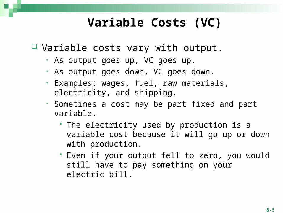
Variable Costs (VC)

Variable costs vary with output.• As output goes up, VC goes up.• As output goes down, VC goes down.• Examples: wages, fuel, raw materials, electricity, and shipping.• Sometimes a cost may be part fixed and part variable.

The electricity used by production is a variable cost because it will go up or down with production.

Even if your output fell to zero, you would still have to pay something on your electric bill.

8-6

Total Cost (TC)

Total cost is the sum of fixed and variable costs.

TC = FC + VC

8-7

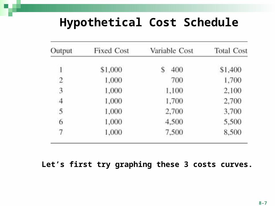
Hypothetical Cost Schedule

Let’s first try graphing these 3 costs curves.

8-8

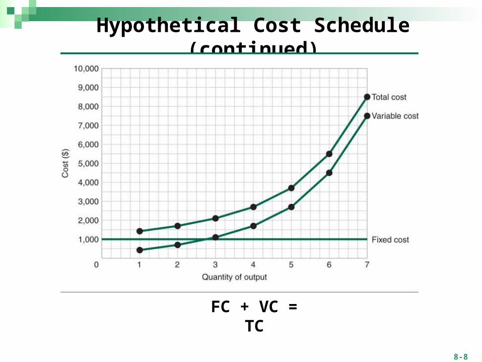
FC + VC = TC

Hypothetical Cost Schedule (continued)

8-9

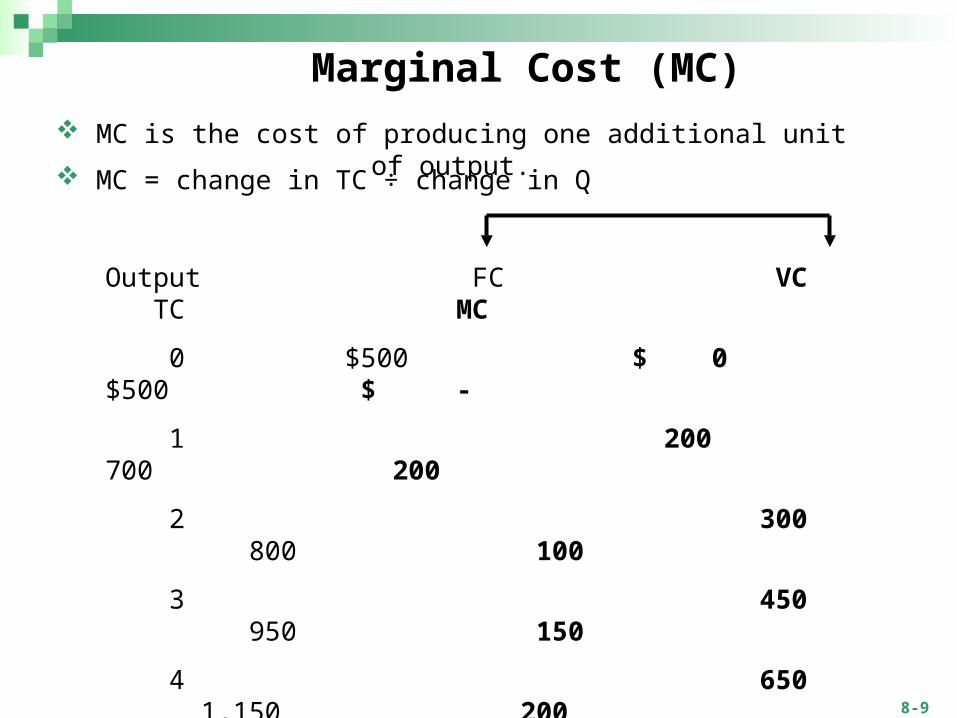
Marginal Cost (MC)

Output FC VC TC MC

0 $500 $ 0 $500 $ -

1 200 700 200

2 300 800 100

3 450 950 150

4 650 1,150 200

5 950 1,450 300

6 1,500 2,000 550

MC is the cost of producing one additional unit of output.

MC = change in TC ÷ change in Q

8-10

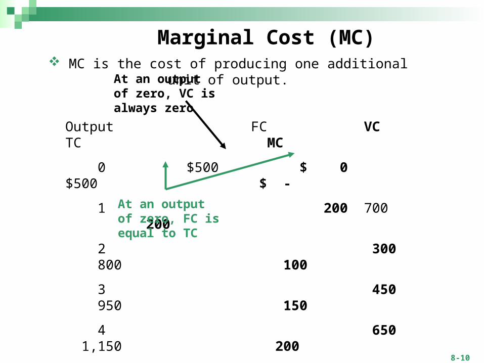
Marginal Cost (MC)

Output FC VC TC MC

0 $500 $ 0 $500 $ -

1 200 700 200

2 300 800 100

3 450 950 150

4 650 1,150 200

5 950 1,450 300

6 1,500 2,000 550

MC is the cost of producing one additional unit of output.At an output of zero, VC is always zero

At an output of zero, FC is equal to TC

8-11

The Short Run (SR) As long as there are any fixed costs, we are in the

short run.• The present time is always the short run.

The short run is the length of time it takes all fixed costs to become variable costs.

• In other words, the length of time it takes to eliminate all fixed costs.

A steel firm might need 10 years to pay off such fixed costs as interest and rent.

Even a grocery store would need a few weeks or months to sublet the store and discharge its other obligations.

8-12

The Long Run (LR)

The long run is the time at which all costs become variable costs.

• Never exists except in theory…you never rally reach the long run.

You will never have a situation in which all your costs are variable.

This would mean no rent, no insurance, no guaranteed salaries, no depreciation, etc.

As you proceed through the short run, you are forced to make decisions that will push the long run farther into the future.

8-13

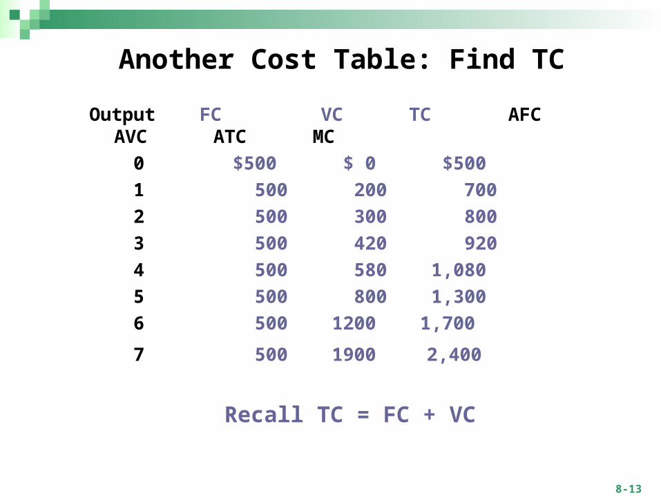
Another Cost Table: Find TC

Output FC VC TC AFC AVC ATC MC

0 $500 $ 0 $500

1 500 200 700

2 500 300 800

3 500 420 920

4 500 580 1,080

5 500 800 1,300

6 500 1200 1,700

7 500 1900 2,400

Recall TC = FC + VC

8-14

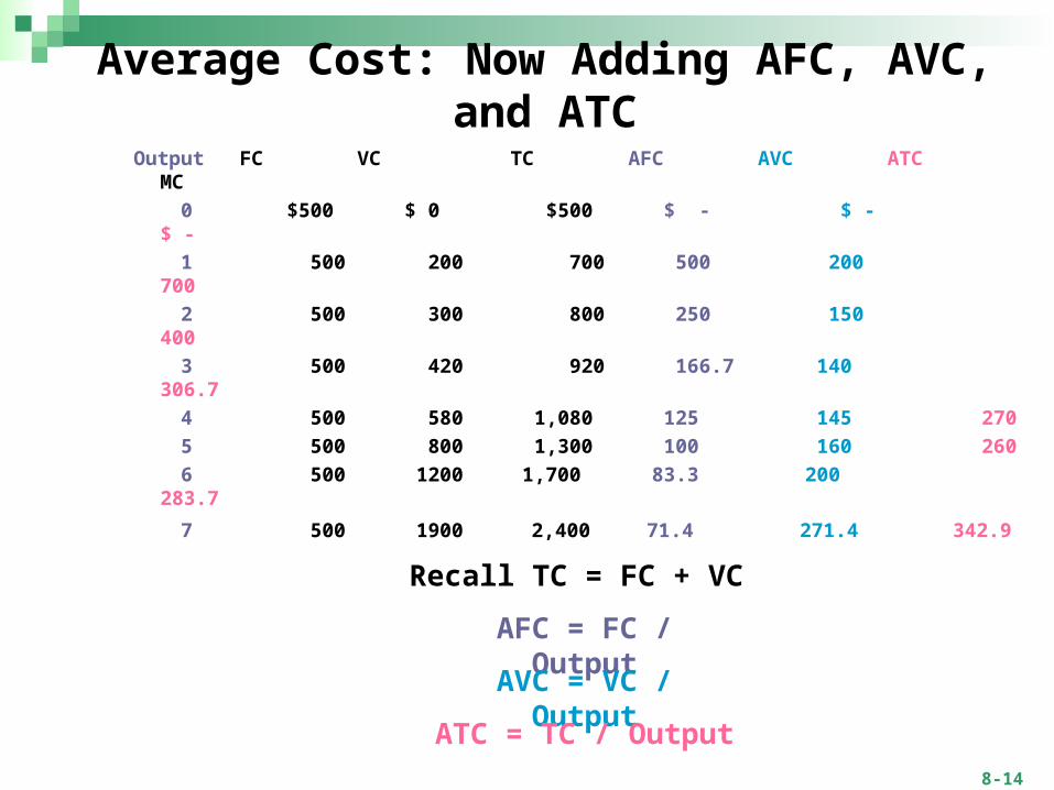
Average Cost: Now Adding AFC, AVC, and ATC

Output FC VC TC AFC AVC ATC MC

0 $500 $ 0 $500 $ - $ - $ -

1 500 200 700 500 200 700

2 500 300 800 250 150 400

3 500 420 920 166.7 140 306.7

4 500 580 1,080 125 145 270

5 500 800 1,300 100 160 260

6 500 1200 1,700 83.3 200 283.7

7 500 1900 2,400 71.4 271.4 342.9

AFC = FC / Output

AVC = VC / Output

ATC = TC / Output

Recall TC = FC + VC

8-15

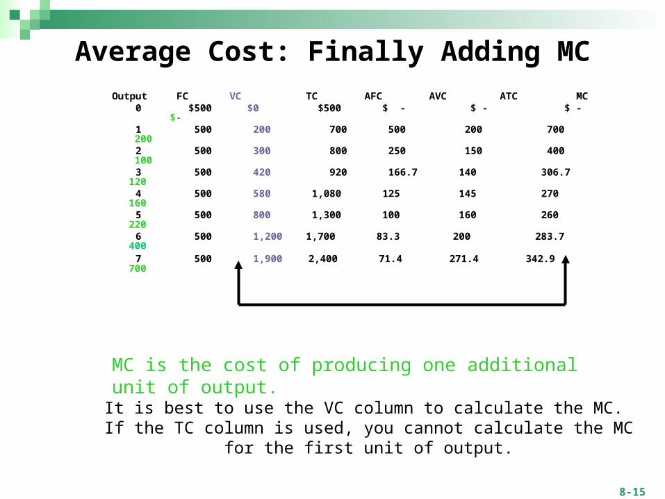
Average Cost: Finally Adding MC

Output FC VC TC AFC AVC ATC MC 0 $500 $0 $500 $ - $ - $ - $- 1 500 200 700 500 200 700 200 2 500 300 800 250 150 400 100 3 500 420 920 166.7 140 306.7 120 4 500 580 1,080 125 145 270 160 5 500 800 1,300 100 160 260 220 6 500 1,200 1,700 83.3 200 283.7 400 7 500 1,900 2,400 71.4 271.4 342.9 700

MC is the cost of producing one additional unit of output.

It is best to use the VC column to calculate the MC. If the TC column is used, you cannot calculate the MC for the first unit of output.

8-16

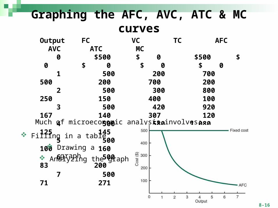
Output FC VC TC AFC AVC ATC MC 0 $500 $ 0 $500 $ 0 $ 0 $ 0 $ 0 1 500 200 700 500 200 700 200 2 500 300 800 250 150 400 100 3 500 420 920 167 140 307 120 4 500 580 1,080 125 145 270 160 5 500 800 1,300 100 160 260 220 6 500 1,200 1,700 83 200 283 400 7 500 1,900 2,400 71 271 343 700

Much of microeconomic analysis involves:

Graphing the AFC, AVC, ATC & MC curves

Filling in a table

Drawing a graph

Analyzing the graph

8-17

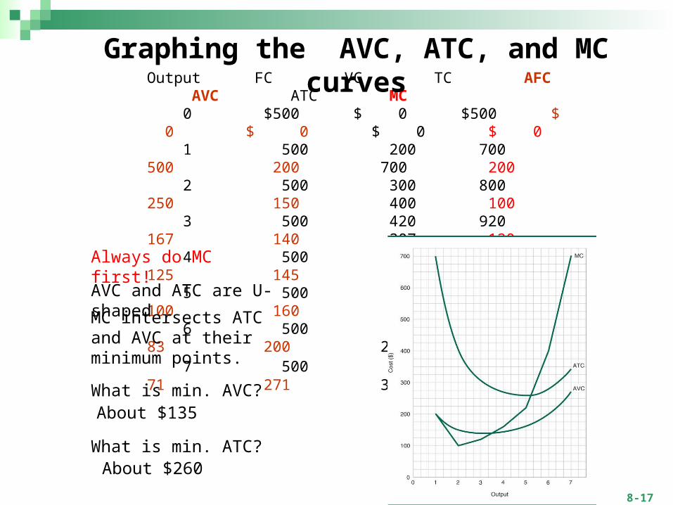
Output FC VC TC AFC AVC ATC MC 0 $500 $ 0 $500 $ 0 $ 0 $ 0 $ 0 1 500 200 700 500 200 700 200 2 500 300 800 250 150 400 100 3 500 420 920 167 140 307 120 4 500 580 1080 125 145 270 160 5 500 800 1300 100 160 260 220 6 500 1200 1700 83 200 283 400 7 500 1900 2400 71 271 343 700

Graphing the AVC, ATC, and MC curves

Always do MC first!

MC intersects ATC and AVC at their minimum points.

What is min. AVC?

What is min. ATC?

AVC and ATC are U-shaped

About $135

About $260

8-18

Minimum AVC: $70 Minimum ATC: $166

Further Discussion: You Try Finding Minimum AVC and ATC points

8-19

The MC curve intersects the ATC and AVC at their minimum points.

Review

8-20

The Production Function and the Law of Diminishing Returns

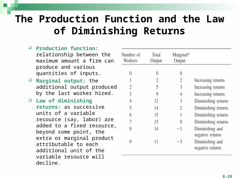
Production function: relationship between the maximum amount a firm can produce and various quantities of inputs.

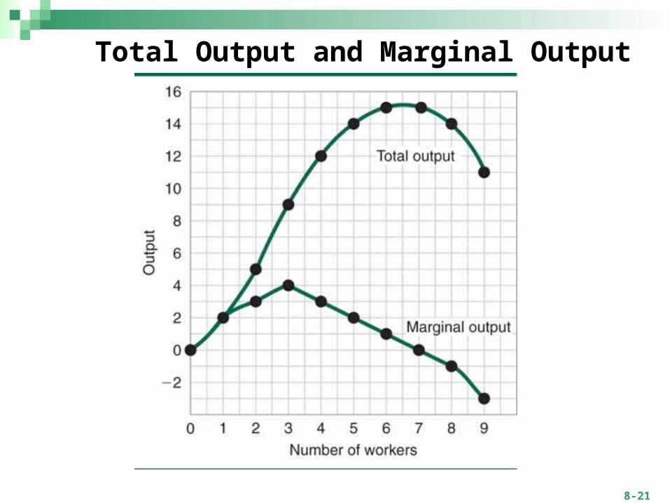
Marginal output: the additional output produced by the last worker hired.

Law of diminishing returns: as successive units of a variable resource (say, labor) are added to a fixed resource, beyond some point, the extra or marginal product attributable to each additional unit of the variable resource will decline.

8-21

Total Output and Marginal Output

8-22

Economies of Scale Economies of scale: the economies of mass

production, which drive down ATC.• Evidenced by the declining part of the ATC curve

In general, we expect large firms to undersell small firms. Reasons are:

• Quantity discounts• Economies of being established• Spreading fixed cost

Economies of scale enable a business to reduce its cost per unit as output expands.

8-23

Diseconomies of Scale

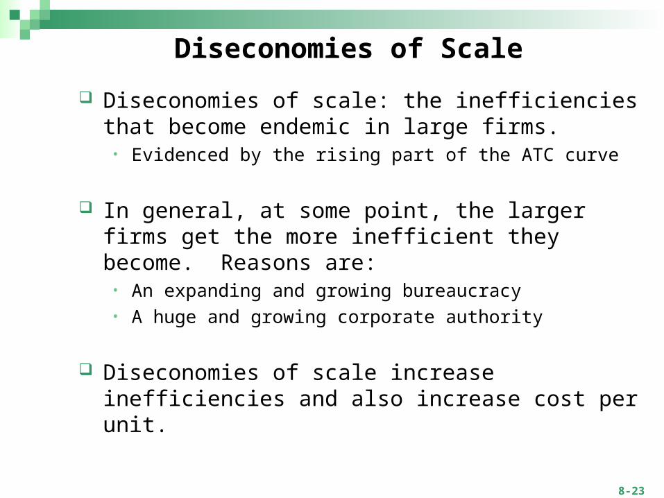
Diseconomies of scale: the inefficiencies that become endemic in large firms.

• Evidenced by the rising part of the ATC curve

In general, at some point, the larger firms get the more inefficient they become. Reasons are:

• An expanding and growing bureaucracy• A huge and growing corporate authority

Diseconomies of scale increase inefficiencies and also increase cost per unit.

8-24

A Summing Up

The overlapping forces of increasing returns and economies of scale drive down ATC.

Eventually, the overlapping forces of diminishing returns and diseconomies of scale push ATC back up again.

The U-shaped ATC is very important in economic analysis and in business strategy.

• What size size plant do we build?• How many workers do we hire?• What is the output at which our firm would operate most

efficiently?

8-25

The Decision to Operate or Shut Down: The Short Run

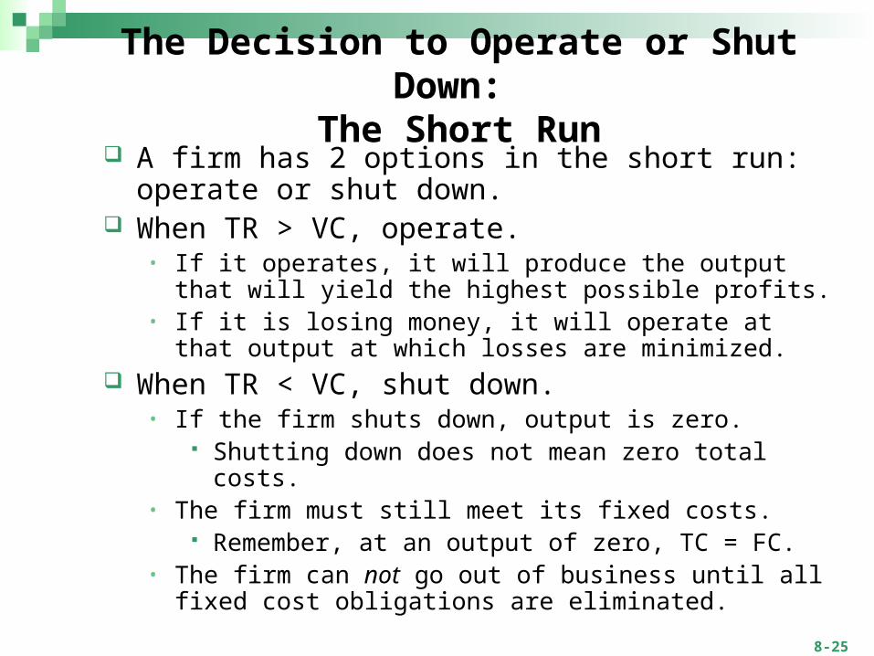
A firm has 2 options in the short run: operate or shut down.

When TR > VC, operate.• If it operates, it will produce the output that will yield the

highest possible profits.• If it is losing money, it will operate at that output at which

losses are minimized. When TR < VC, shut down.

• If the firm shuts down, output is zero. Shutting down does not mean zero total costs.

• The firm must still meet its fixed costs. Remember, at an output of zero, TC = FC.

• The firm can not go out of business until all fixed cost obligations are eliminated.

8-26

Summary Table: Let’s Try 3 Problems

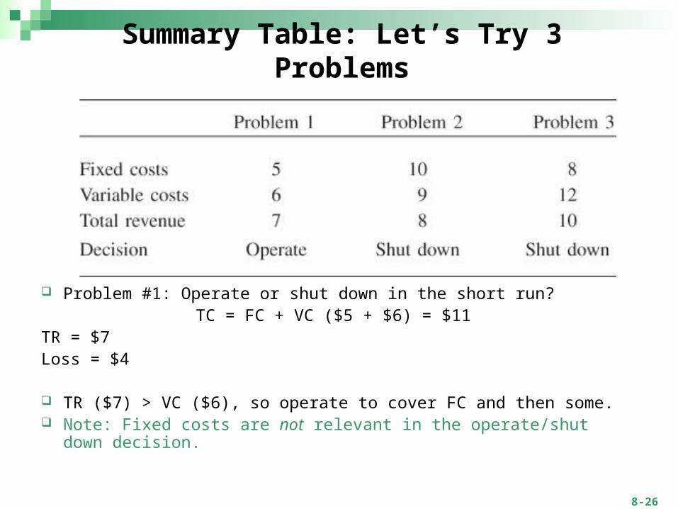
Problem #1: Operate or shut down in the short run?TC = FC + VC ($5 + $6) = $11

TR = $7Loss = $4

TR ($7) > VC ($6), so operate to cover FC and then some. Note: Fixed costs are not relevant in the operate/shut down decision.

8-27

Summary Table: Let’s Try 3 Problems

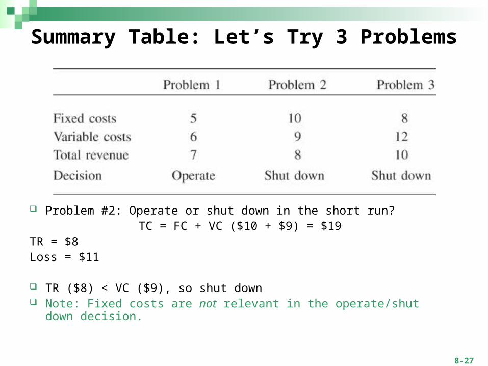
Problem #2: Operate or shut down in the short run?TC = FC + VC ($10 + $9) = $19

TR = $8Loss = $11

TR ($8) < VC ($9), so shut down Note: Fixed costs are not relevant in the operate/shut down decision.

8-28

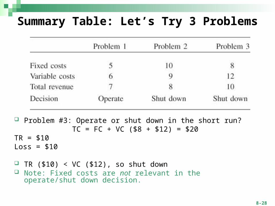
Summary Table: Let’s Try 3 Problems

Problem #3: Operate or shut down in the short run?TC = FC + VC ($8 + $12) = $20

TR = $10Loss = $10

TR ($10) < VC ($12), so shut down Note: Fixed costs are not relevant in the operate/shut down decision.

8-29

The Decision to Stay In or Go Out of Business: The Long Run

In the long run, firms must decide to stay in business or go out of business.

• The firm will stay in business if the total revenue is greater than its total cost.

• The firm will go out of business if the total cost exceeds total revenue.

Going out of business means that all fixed cost obligations are met.

Does everybody who is losing money go out of business?

• Eventually (most sooner rather than later).• There are always exceptions to the rule.

8-30

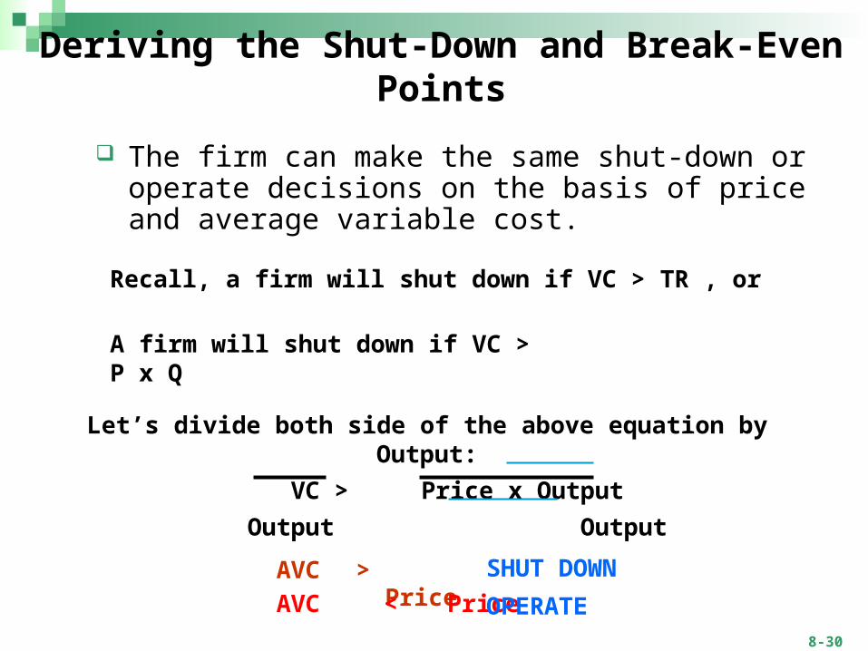
Deriving the Shut-Down and Break-Even Points

The firm can make the same shut-down or operate decisions on the basis of price and average variable cost.

Recall, a firm will shut down if VC > TR , or

A firm will shut down if VC > P x Q

Let’s divide both side of the above equation by Output:

VC > Price x Output

Output Output

AVC > Price SHUT DOWN

AVC < Price OPERATE

8-31

Deriving the Shut-Down and Break-Even Points

The firm can make the same stay in business or go out of business decisions on the basis of price and average total cost.

Recall, a firm will go out of business if TC > TR , or

A firm will go out of business if TC > P x Q

Let’s divide both side of the above equation by Output:

TC > Price x Output

Output Output

ATC > Price GO OUT OF BUSINESS

ATC < Price OPERATE

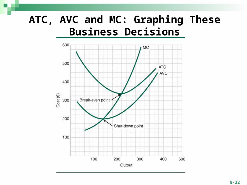
8-32

ATC, AVC and MC: Graphing These Business Decisions

8-33

Questions for Thought and Discussion

Pretend you are the owner of a coffee house. What would be the difference between shutting down and going out of business?

• What are the fixed costs?• What are the variable costs?

Why does it take longer to go out of business than to shut down?

8-34

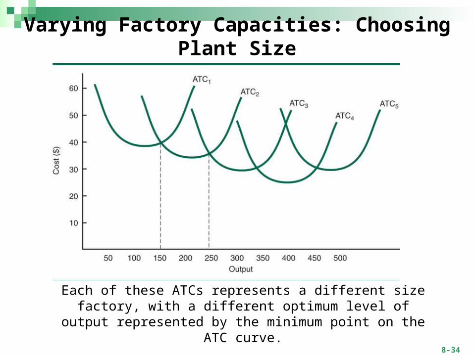
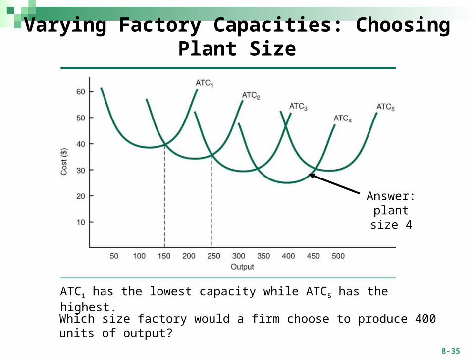
Varying Factory Capacities: Choosing Plant Size

Each of these ATCs represents a different size factory, with a different optimum level of output represented by the minimum

point on the ATC curve.

8-35

Varying Factory Capacities: Choosing Plant Size

ATC1 has the lowest capacity while ATC5 has the highest.

Which size factory would a firm choose to produce 400 units of output?

Answer: plant size 4

8-36

Varying Factory Capacities: Choosing Plant Size

Changes in plant size are long run changes. In the long run, a firm could be virtually any size provided it has the requisite

financing.

8-37

Current Issue: Wedding Hall or City Hall? Every wedding, big or small incurs fixed cost and

variable cost.• Fixed costs: flowers, photographer, the wedding hall, the

gowns, the videographer, tux rentals, clergy.• Variable costs: food and drinks; the number of guest will affect

the size of the wedding hall.

A relatively small wedding that cost $20,000 and might pull in gifts worth $10,000.

A much larger wedding might cost $100,000 and might pull in gifts worth $50,000.

Do you go for the large wedding or smaller one?