Citation: Idso, C.D., Legates, D. and Singer, S.F. 2019. Climate Science. In: Climate Change Reconsidered II: Fossil Fuels. Nongovernmental International Panel on Climate Change. Arlington Heights, IL: The Heartland Institute.

671

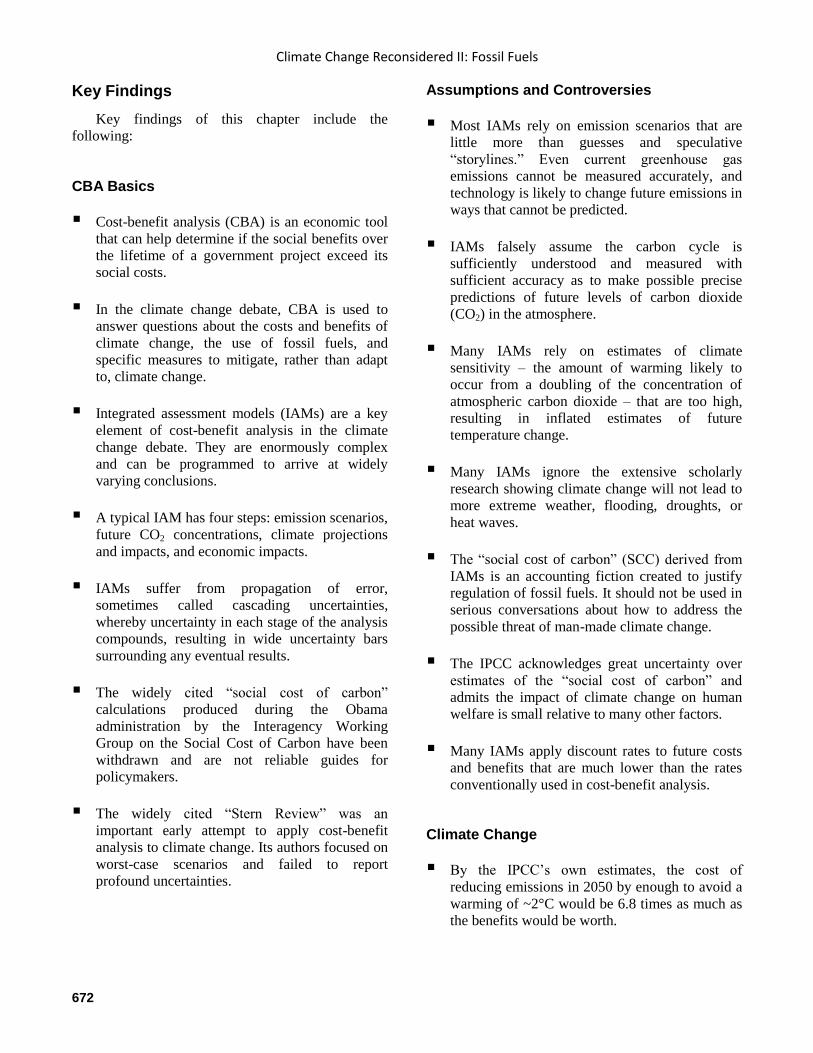
8 Cost-Benefit Analysis

Chapter Lead Authors: Roger Bezdek, Ph.D., Christopher Monckton of Brenchley Contributors: Joseph L. Bast, Barry Brill, OBE, JP, Kevin Dayaratna, Ph.D., Bryan Leyland, M.Sc. Reviewers: David Archibald, Patrick Frank, Ph.D., Donald Hertzmark, Ph.D., Paul McFadyen, Ph.D., Patrick Michaels, Ph.D., Robert Murphy, Ph.D., Charles N. Steele, Ph.D., David Stevenson

Key Findings Introduction 8.1 CBA Basics 8.1.1 Use in the Climate Change Debate 8.1.2 Integrated Assessment Models 8.1.2.1 Background and Structure 8.1.2.2 Propagation of Error 8.1.3 IWG Reports 8.1.4 Stern Review 8.1.5 Conclusion 8.2 Assumptions and Controversies 8.2.1 Emission Scenarios 8.2.2 Carbon Cycle 8.2.3 Climate Sensitivity 8.2.4 Climate Impacts 8.2.5 Economic Impacts 8.2.5.1 The IPCC’s Findings 8.2.5.2 Discount Rates

8.3 Climate Change 8.3.1 The IPCC’s Findings 8.3.2 DICE and FUND Models 8.3.3 A Negative SCC 8.4 Fossil Fuels 8.4.1 Impacts of Fossil Fuels 8.4.2 Cost of Mitigation

8.4.2.1 High Cost of Reducing Emissions

8.4.2.2 High Cost of Reducing Energy Consumption 8.4.3 New CBAs 8.5 Regulations 8.5.1 Common Variables 8.5.2 Case-specific Variables 8.5.3 Outputs of the CBA Model 8.5.4 CBA Model 8.5.5 Model Applied 8.5.6 Results Discussed 8.6 Conclusion

Climate Change Reconsidered II: Fossil Fuels

672

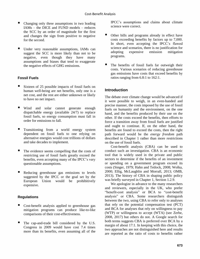
Key Findings

Key findings of this chapter include the

following:

CBA Basics

Cost-benefit analysis (CBA) is an economic tool

that can help determine if the social benefits over

the lifetime of a government project exceed its

social costs.

In the climate change debate, CBA is used to

answer questions about the costs and benefits of

climate change, the use of fossil fuels, and

specific measures to mitigate, rather than adapt

to, climate change.

Integrated assessment models (IAMs) are a key

element of cost-benefit analysis in the climate

change debate. They are enormously complex

and can be programmed to arrive at widely

varying conclusions.

A typical IAM has four steps: emission scenarios,

future CO2 concentrations, climate projections

and impacts, and economic impacts.

IAMs suffer from propagation of error,

sometimes called cascading uncertainties,

whereby uncertainty in each stage of the analysis

compounds, resulting in wide uncertainty bars

surrounding any eventual results.

The widely cited “social cost of carbon”

calculations produced during the Obama

administration by the Interagency Working

Group on the Social Cost of Carbon have been

withdrawn and are not reliable guides for

policymakers.

The widely cited “Stern Review” was an

important early attempt to apply cost-benefit

analysis to climate change. Its authors focused on

worst-case scenarios and failed to report

profound uncertainties.

Assumptions and Controversies

Most IAMs rely on emission scenarios that are

little more than guesses and speculative

“storylines.” Even current greenhouse gas

emissions cannot be measured accurately, and

technology is likely to change future emissions in

ways that cannot be predicted.

IAMs falsely assume the carbon cycle is

sufficiently understood and measured with

sufficient accuracy as to make possible precise

predictions of future levels of carbon dioxide

(CO2) in the atmosphere.

Many IAMs rely on estimates of climate

sensitivity – the amount of warming likely to

occur from a doubling of the concentration of

atmospheric carbon dioxide – that are too high,

resulting in inflated estimates of future

temperature change.

Many IAMs ignore the extensive scholarly

research showing climate change will not lead to

more extreme weather, flooding, droughts, or

heat waves.

The “social cost of carbon” (SCC) derived from

IAMs is an accounting fiction created to justify

regulation of fossil fuels. It should not be used in

serious conversations about how to address the

possible threat of man-made climate change.

The IPCC acknowledges great uncertainty over

estimates of the “social cost of carbon” and

admits the impact of climate change on human

welfare is small relative to many other factors.

Many IAMs apply discount rates to future costs

and benefits that are much lower than the rates

conventionally used in cost-benefit analysis.

Climate Change

By the IPCC’s own estimates, the cost of

reducing emissions in 2050 by enough to avoid a

warming of ~2°C would be 6.8 times as much as

the benefits would be worth.

Cost-Benefit Analysis

673

Changing only three assumptions in two leading

IAMs – the DICE and FUND models – reduces

the SCC by an order of magnitude for the first

and changes the sign from positive to negative

for the second.

Under very reasonable assumptions, IAMs can

suggest the SCC is more likely than not to be

negative, even though they have many

assumptions and biases that tend to exaggerate

the negative effects of GHG emissions.

Fossil Fuels

Sixteen of 25 possible impacts of fossil fuels on

human well-being are net benefits, only one is a

net cost, and the rest are either unknown or likely

to have no net impact.

Wind and solar cannot generate enough

dispatchable energy (available 24/7) to replace

fossil fuels, so energy consumption must fall in

order for emissions to fall.

Transitioning from a world energy system

dependent on fossil fuels to one relying on

alternative energies would cost trillions of dollars

and take decades to implement.

The evidence seems compelling that the costs of

restricting use of fossil fuels greatly exceed the

benefits, even accepting many of the IPCC’s very

questionable assumptions.

Reducing greenhouse gas emissions to levels

suggested by the IPCC or the goal set by the

European Union would be prohibitively

expensive.

Regulations

Cost-benefit analysis applied to greenhouse gas

mitigation programs can produce like-to-like

comparisons of their cost-effectiveness.

The cap-and-trade bill considered by the U.S.

Congress in 2009 would have cost 7.4 times

more than its benefits, even assuming all of the

IPCC’s assumptions and claims about climate

science were correct.

Other bills and programs already in effect have

costs exceeding benefits by factors up to 7,000.

In short, even accepting the IPCC’s flawed

science and scenarios, there is no justification for

adopting expensive emission mitigation

programs.

The benefits of fossil fuels far outweigh their

costs. Various scenarios of reducing greenhouse

gas emissions have costs that exceed benefits by

ratios ranging from 6.8:1 to 162:1.

Introduction

The debate over climate change would be advanced if

it were possible to weigh, in an even-handed and

precise manner, the costs imposed by the use of fossil

fuels on humanity and the environment, on the one

hand, and the benefits produced by their use on the

other. If the costs exceed the benefits, then efforts to

force a transition away from fossil fuels are justified

and ought to continue. If, on the other hand, the

benefits are found to exceed the costs, then the right

path forward would be the energy freedom path

described in Chapter 1 rather than more restrictions

on the use of fossil fuels.

Cost-benefit analysis (CBA) can be used to

conduct such an investigation. CBA is an economic

tool that is widely used in the private and public

sectors to determine if the benefits of an investment

or spending on a government program exceed its

costs (Singer, 1979; Hahn and Tetlock, 2008; Wolka,

2000; Ellig, McLaughlin and Morrall, 2013; OMB,

2013). The history of CBA in shaping public policy

was briefly surveyed in Chapter 1, Section 1.2.9.

We apologize in advance to the many researchers

and reviewers, especially in the UK, who prefer

“benefit-cost analysis” or BCA to “cost-benefit

analysis” or CBA. Some researchers distinguish

between the two, using CBA to refer only to analyses

that rely on the potential compensation test (PCT)

and BCA for analyses that rely on willingness to pay

(WTP) or willingness to accept (WTA) (see Zerbe,

2008, 2017) but others do not. A Google search for

both terms suggests CBA is preferred over BCA by a

margin of about 17:1. In keeping with this choice, the

two approaches are not distinguished here and results

are reported as the ratio of costs to benefits rather

Climate Change Reconsidered II: Fossil Fuels

674

than benefits to costs. Except for the final section,

where the editors defer to the wishes of a chapter lead

author.

Cost-benefit analysis is a complex endeavor

typically involving subjective choices about what

data to include and what to leave out, how to weigh

evidence, and how to interpret results. The discipline

is complicated enough to merit its own society, the

Society for Benefit-Cost Analysis, and its own

journal, Journal of Benefit-Cost Analysis. Section 8.1

begins with a brief tutorial on the application of CBA

to the climate change debate. It is followed by an

introduction to integrated assessment models (IAMs),

an explanation of their biggest shortcoming (the

“propagation of error” or cascading uncertainty), and

reviews of CBAs of global warming produced by the

Interagency Working Group on the Social Cost of

Carbon (since disbanded) and the British Stern

Review.

Section 8.2 examines the assumptions and biases

that underlie IAMs. Tracking the order of “blocks” or

“modules” in IAMs and drawing on research

presented in previous chapters, it shows how errors or

uncertainties in choosing emission scenarios,

estimating the amount of carbon dioxide that stays in

the atmosphere, the likelihood of increases in

flooding and extreme weather, and other inputs

render IAMs too unreliable to be of any use to

policymakers.

Section 8.3 shows how two leading IAMs – the

DICE and FUND models – rely on inaccurate

equilibrium climate sensitivity rates, low discount

rates, and a too-long time horizon (300 years).

Correcting only these errors reveals the SCC is most

likely negative, even accepting all of the IPCC’s

other errors and faulty assumptions. In other words,

the social benefits of anthropogenic GHG emissions

exceed their social cost.

Sections 8.4 summarizes the extensive literature

reviews on the impacts of fossil fuels on human well-

being conducted for earlier chapters in a single table.

It reveals 16 of 25 possible impacts are positive (net

benefits), only one is negative (net cost), and the rest

are unknown or produce benefits and costs that are

likely to offset each other. It presents cost-benefit

analyses showing the cost of ending humanity’s

reliance on fossil fuels would be between 32 and 162

times as much as the hypothetical benefits of a

slightly cooler world in 2050 and beyond.

Section 8.5 presents a formula for calculating the

cost-effectiveness of GHG mitigation programs using

the IPCC’s own data and assumptions to produce

like-to-like comparisons. The formula reveals a

sample of proposed and existing programs has cost-

benefit ratios ranging from 7.4:1 to 7,000:1,

suggesting that current regulations, subsidies, and tax

schemes aimed at reducing GHG emissions are not

justified by their social benefits.

Section 8.6 offers a brief conclusion. According

to the authors, CBA reveals the global war on energy

freedom, which commenced in earnest in the 1980s

and reached a fever pitch in the second decade of the

twenty-first century, was never founded on sound

science or economics. They urge the world’s

policymakers to acknowledge this truth and end that

war.

References

Ellig, J., McLaughlin, P.A., and Morrall, J. 2013.

Continuity, change, and priorities: The quality and use of

regulatory analysis across US administrations. Regulation

and Governance 7 (2).

Hahn, R.W. and Tetlock, P.C. 2008. Has economic

analysis improved regulatory decisions? Journal of

Economic Perspectives 22: 1. 67–84.

OMB. 2013. U.S. Office of Management and Budget.

Draft report to Congress on the benefits and costs of

federal regulations and agency compliance with the

Unfunded Mandates Reform Act.

Singer, S.F. 1979. Cost Benefit Analysis as an Aid to

Environmental Decision Making. McLean, VA: The

MITRE Corporation.

Wolka, K. 2000. Chapter 8. Analysis and modeling,

Section 8.9 economics, in Lehr, J.H. (Ed.) Standard

Handbook of Environmental, Science, Health, and

Technology. New York, NY: McGraw-Hill, 8.122–8.133.

Zerbe, R.O. 2008. Ethical benefit cost analysis as art and

science: ten rules for benefit-cost analysis. University of

Pennsylvania Journal of Law and Social Change 12 (1).

Zerbe, R.O. 2017. A distinction between benefit-cost

analysis and cost benefit analysis, moral reasoning and a

justification for benefit-cost analysis. Seattle, WA: Evans

School of Public Policy and Governance, University of

Washington.

Society for Cost Benefit Analysis, n.d. (website). Accessed

November 17, 2018.

Cost-Benefit Analysis

675

8.1 CBA Basics

Cost-benefit analysis (CBA) is an economic

tool that can help determine if the social

benefits over the lifetime of a government

project exceed its social costs.

Section 8.1.1 describes how cost-benefit analysis can

be used to answer four key questions in the climate

change debate. Section 8.1.2 provides background

and an overview of the structure of integrated

assessment models (IAMs) and describes how the

“propagation of error” or cascading uncertainty

renders their outputs unreliable. Sections 8.1.3 and

8.1.4 critique two of the best known attempts to apply

CBA to climate change, the U.S. Interagency

Working Group on the Social Cost of Carbon (since

disbanded) and the British Stern Review. Section

8.1.5 presents a brief conclusion.

8.1.1 Use in the Climate Change Debate

In the climate change debate, CBA is used to answer

four distinct questions:

1. Do the benefits from the use of fossil fuels, such

as the increase in per-capita income made

possible by affordable energy and higher

agricultural output due to higher carbon dioxide

(CO2) levels in the atmosphere, exceed the costs

it may have imposed, such as reduced air quality

and, if they contribute to climate change, damage

and harm from floods, droughts, or other severe

weather events? (Bezdek, 2014)

2. Do the social benefits of either fossil fuels or

climate change exceed the social cost – that is, do

the positive externalities produced by the private

use of fossil fuels exceed the negative

externalities imposed on others? This is often

called the “social cost of carbon” (SCC),

calculated as the welfare loss associated with

each additional metric ton of CO2 emitted. (Tol,

2011)

3. Will the benefits of a particular program to

reduce greenhouse gas emissions or sequester

CO2 by planting trees or injecting the gas into

wells for underground storage exceed the costs

incurred in implementing that program?

(Monckton, 2016)

4. Is the cost-benefit ratio of a particular program to

mitigate climate change higher or lower than the

cost-benefit ratio of adapting to climate change

by investing in stronger levees and dams, finding

alternative sources of water, or “hardening”

critical infrastructure? This is the “mitigate

versus adapt” question that is frequently

referenced in the Working Group II contribution

to the IPCC’s Fifth Assessment Report (AR5)

(e.g., IPCC, 2014a, Chapter 10, pp. 665–666,

669, 679).

Regarding the first question, about the total

private and social costs and benefits of the use of

fossil fuels, Chapters 3 and 4 showed how fossil fuels

made possible three Industrial Revolutions which in

turn made possible large increases in human

population, per-capita income, and lifespan (Bradley,

2000; Smil, 2005, 2006; Goklany, 2007; Bryce, 2010,

2014; Gordon, 2016). The benefits continue to

accumulate today as cleaner-burning fossil fuels

bring electricity to third-world countries and replace

wood and dung as sources of heat in homes (Yadama,

2013; Bezdek, 2014). How much of the benefits of

that economic transformation should be counted as

“private” versus “social” benefits is not immediately

apparent, but those benefits cannot be ignored

entirely.

Rising atmospheric carbon dioxide

concentrations and higher temperatures produce other

benefits such as higher agricultural productivity,

expanded ranges for most terrestrial animals having

economic value such as livestock, and lower levels of

human mortality and morbidity traditionally caused

by exposure to cold temperatures (see Chapters 4 and

5 and Idso, 2013 for a detailed review of this

literature). These well-known and observable benefits

must be compared and weighed against cost estimates

appearing in CBAs that are much less certain or well

documented, many of which could even be judged

conjectural.

Forward-looking CBAs must be based on

reasonably accurate forecasts of future climate

conditions. This requires climate models that take

explicit, quantitative account of the principal relevant

results in climatology, notably the radiative-forcing

functions of CO2 and other greenhouse gases and the

various values of the climate sensitivity parameter.

Current climate models have not shown much

promise in this regard, as deomonstrated in Chapter

2, Section 2.2.2 (and see Fyfe et al., 2013; McKitrick

and Christy, 2018). CBAs also require economic

models that can predict future changes in per-capita

Climate Change Reconsidered II: Fossil Fuels

676

income, energy supply and demand, rate of

technological innovation, economic growth rates in

the developed and developing worlds, demographic

trends, changes in land use and lifestyles, greenhouse

gases other than carbon dioxide, and even political

trends such as whether civil and economic freedoms

are likely to expand or contract in various parts of the

world (van Kooten, 2013).

The IPCC claims it can resolve all these

uncertainties. In the Working Group III contribution

to AR5, the IPCC says “a likely chance to keep

average global temperature change below 2°C

relative to pre-industrial levels” would require “lower

global GHG emissions in 2050 than in 2010, 40% to

70% lower globally, and emissions levels near zero

GtCO2eq or below in 2100” (IPCC, 2014b, pp. 10,

12). Since fossil fuels are responsible for

approximately 80% of anthropogenic greenhouse gas

emissions, this would require gradually phasing out

the use of fossil fuels and banning their use entirely

by 2100.

Any effort to calculate the costs and benefits of

future climate change confronts fundamental

problems inherent in making forecasts in the absence

of complete understanding of underlying causes and

effects. In such cases, the most reliable method of

forecasting is to project a simple linear continuation

of past trends (Armstrong, 2001), but this plainly is

not what is done by the IPCC or the authors of the

models on which it relies. An audit of the IPCC’s

Fourth Assessment Report conducted by experts in

scientific forecasting found “the forecasting

procedures that were described [in sufficient detail to

be evaluated] violated 72 principles” of scientific

forecasting (Green and Armstrong, 2007). The

authors found no evidence the scientists involved in

making the IPCC’s forecasts were even aware of the

literature on scientific forecasting.

Cost-benefit analysis of future climate change

also must address the effects of dematerialization. As

the research by Wernick and Ausubel (2014), Smil

(2013), and others cited in Chapter 5 demonstrates,

technological change is lowering the energy- and

carbon-intensity of manufacturing and goods and

services generally in the United States and globally,

meaning future emission levels may be lower or less

certain than is presently assumed. The cost of

reducing emissions is likely to be lower in the future

as well, as new technologies emerge to capture and

sequester carbon dioxide or generate energy or

consumer goods without emissions. As Mendelsohn

(2004) writes, “there is no question but that we will

learn a great deal about controlling greenhouse gases

and about climate change over even the next few

decades. The optimal policy is to commit to only

what one will do in the near term. Every decade, this

policy should be reexamined in light of new

evidence. Once the international community has a

viable program in place, it is easy to imagine the

community being able to adjust their policies based

on what new information is forthcoming” (p. 47).

Comparing the costs and benefits of specific

mitigation efforts, the third question, requires CBA

methodologies that are case-specific, which means

they can be applied to specific mitigation projects

such as a carbon tax, a carbon trading program,

investment in solar photo-voltaic systems, or

subsidizing electric cars (Monckton, 2014, 2016).

Conducting CBAs of mitigation strategies is

complicated by the fact that the possible benefits

from mitigation will not be apparent until many years

into the future – the models used often claim to be

accurate and policy-relevant 100 years and even

longer – even though the costs will be incurred

immediately and will be ongoing. This makes

choosing an appropriate discount rate – the subject of

Section 8.2.5.2 – critical to producing an accurate

evaluation.

There is considerable uncertainty regarding

whether man-made emissions will ever cause a

contribution to atmospheric warming of more than 1°

or 2°C. Some experts believe costs may begin to

exceed benefits if the contribution of man-made

emissions is a temperature rise exceeding 2.5°C

above pre-industrial levels (Mendelsohn and

Williams, 2004; Tol, 2009; Doiron, 2014). If

temperatures stop rising before or around that point,

due to natural feedbacks or simply because man no

longer is producing large quantities of greenhouse

gases or because the climate sensitivity to greenhouse

gases is lower than the IPCC projects, then enormous

expenditures spanning generations will have been

entirely wasted.

Because forcing a transition away from fossil

fuels to alternative fuels requires raising the price of

energy, and the price of energy is closely related to

the rate of economic growth, actions taken today to

reduce emissions will reduce the wealth of future

generations. Thus, investing today to avoid or delay a

future hazard that may or may not even materialize

may undermine the ability of future generations to

cope with climate change (whether natural or man-

made) or make further progress in protecting the

natural environment from other, real, threats.

The fourth question, which asks if mitigation is

preferable to adaptation, is often overlooked by

Cost-Benefit Analysis

677

scientists and policymakers alike. Environmentalists

who are predisposed to oppose initiatives that shape

or alter the natural world view adaptation strategies

as insufficient and likely to result in doubling down

on past bad behavior that could make the situation

worse rather than better (Orr, 2012). However, if

future climate change is gradual, unlikely to reach the

levels feared by some proponents of the hypothesis,

or unlikely to be accompanied by many of the

negative impacts thought to occur, then adaptation

would indeed be the preferred strategy.

While the cost of adaptation to unmitigated

warming is not always case-specific, since it may

consist of countless choices made by similarly

countless individuals over long periods of time, the

cost of mitigation projects can be assessed case by

case. This could make direct cost-benefit ratio

comparisons of mitigation strategies with adaptation

difficult, unless the cost of adaptation to unmitigated

global warming can be shown to be lower than even

the best mitigation strategies.

The complexity of climate science and

economics makes conducting any of these CBAs a

difficult and perhaps even impossible challenge

(Ceronsky et al., 2011; Pindyck, 2013). In a candid

statement alluding to the many difficulties associated

with determining the “social cost of carbon,”

Weitzman remarked, “the economics of climate

change is a problem from hell,” adding that “trying to

do a benefit-cost analysis (BCA) of climate change

policies bends and stretches the capability of our

standard economist’s toolkit up to, and perhaps

beyond, the breaking point” (Weitzman, 2015).

References

Armstrong, J.S. 2001. Principles of Forecasting – A

Handbook for Researchers and Practitioners. Norwell,

MA: Kluwer Academic Publishers.

Bezdek, R.H. 2014. The Social Costs of Carbon? No, the

Social Benefits of Carbon. Oakton, VA: Management

Information Services, Inc.

Bradley, R.L. 2000. Julian Simon and the Triumph of

Energy Sustainability. Washington, DC: American

Legislative Exchange Council.

Bryce, R. 2010. Power Hungry: The Myths of ‘Green’

Energy and the Real Fuels of the Future. New York, NY:

PublicAffairs.

Bryce, R. 2014. Smaller Faster Lighter Denser Cheaper.

New York, NY: PublicAffairs.

Ceronsky, M., Anthoff, D., Hepburn, C., and Tol, R.S.J.

2011. Checking the price tag on catastrophe: the social

cost of carbon under non-linear climate response. ESRI

Working Paper No. 392. Dublin, Ireland: Economic and

Social Research Institute.

Doiron, H.H. 2014. Bounding GHG climate sensitivity for

use in regulatory decisions. The Right Climate Stuff

(website). February.

Fyfe, J.C., Gillett, N.P., and Zwiers, F.W. 2013.

Overestimated global warming over the past 20 years.

Nature Climate Change 3: 767–9.

Goklany, I.M. 2007. The Improving State of the World:

Why We’re Living Longer, Healthier, More Comfortable

Lives on a Cleaner Planet. Washington, DC: Cato

Institute.

Gordon, R.J. 2016. The Rise and Fall of American Growth.

Princeton, NJ: Princeton University Press.

Green, K.C. and Armstrong, J.S. 2007. Global warming:

forecasts by scientists versus scientific forecasts. Energy

and Environment 18: 997–1021.

Idso, C.D. 2013. The Positive Externalities of Carbon

Dioxide. Tempe, AZ: Center for the Study of Carbon

Dioxide and Global Change.

IPCC. 2014a. Intergovernmental Panel on Climate Change.

Climate Change 2014: Impacts, Adaptation, and

Vulnerability. Contribution of Working Group II to the

Fifth Assessment Report of the Intergovernmental Panel

on Climate Change. New York, NY: Cambridge

University Press.

IPCC. 2014b. Intergovernmental Panel on Climate

Change. Climate Change 2014: Mitigation of Climate

Change. Contribution of Working Group III to the Fifth

Assessment Report of the Intergovernmental Panel on

Climate Change. New York, NY: Cambridge University

Press.

McKitrick, R. and Christy, J. 2018. A Test of the tropical

200‐ to 300‐hPa warming rate in climate models. Earth

and Space Science 5 (9).

Mendelsohn, R. 2004. The challenge of global warming.

Opponent paper on climate change. In: Lomborg, B. (Ed.)

Global Crises, Global Solutions. Cambridge, MA:

Cambridge University Press.

Mendelsohn, R. and Williams, L. 2004. Comparing

forecasts of the global impacts of climate change.

Mitigation and Adaptation Strategies for Global Change 9:

315–33.

Climate Change Reconsidered II: Fossil Fuels

678

Monckton, C. 2014. To Mitigate or to Adapt? Inputs from

Mainstream Climate Physics to Mitigation Benefit-Cost

Appraisal. Haymarket, VA: Science and Public Policy

Institute.

Monckton, C. 2016. Chapter 10. Is CO2 mitigation cost

effective? In: Easterbrook, D. (Ed.) Evidence-Based

Climate Science. Second Edition. Cambridge, MA:

Elsevier, Inc.

Orr, D.W. 2012. Down to the Wire: Confronting Climate

Collapse. New York, NY: Oxford University Press.

Pindyck, R.S. 2013. Pricing carbon when we don’t know

the right price. Regulation 36 (2): 43–6.

Smil, V. 2005. Creating the Twentieth Century: Technical

Innovations of 1867–1914 and Their Lasting Impact. New

York, NY: Oxford University Press, Inc.

Smil, V. 2006. Transforming the Twentieth Century:

Technical Innovations and Their Consequences. New

York, NY: Oxford University Press, Inc.

Smil, V. 2013. Making the Modern World: Materials and

Dematerialization. New York, NY: Wiley.

Tol, R.S.J. 2009. The economic effects of climate change.

Journal of Economic Perspectives 23 (2): 29–51.

Tol, R.S.J. 2011. The social cost of carbon. Annual Review

of Resource Economics 3: 419–43.

van Kooten, G.C. 2013. Climate Change, Climate Science

and Economics: Prospects for an Alternative Energy

Future. New York, NY: Springer.

Weitzman, M.L. 2015. A review of William Nordhaus’

“The climate casino: risk, uncertainty, and economics for a

warming world. Review of Environmental Economics and

Policy 9: 145–56.

Wernick, I. and Ausubel, J.H. 2014. Making Nature

Useless? Global Resource Trends, Innovation, and

Implications for Conservation. Washington, DC:

Resources for the Future. November.

Yadama, G.N. 2013. Fires, Fuels, and the Fate of

3 Billion: The State of the Energy Impoverished. New

York, NY: Oxford University Press.

8.1.2 Integrated Assessment Models

Integrated assessment models (IAMs) are a

key element of cost-benefit analysis in the

climate change debate. They are enormously

complex and can be programmed to arrive at

widely varying conclusions.

Integrated assessment models (IAMs), as they are

used in the climate change debate, are mathematical

constructs that provide a framework for combining

knowledge from a wide range of disciplines, in

particular climate science and economics, to measure

economic damages associated with carbon dioxide

(CO2)-induced climate change. In public discourse as

well as academic research, this measure is often

referred to as the “social cost of carbon” (SCC)

which Nordhaus (2011) defines as “the economic

cost caused by an additional ton of carbon dioxide

emissions (or more succinctly carbon) or its

equivalent. In a more precise definition, it is the

change in the discounted value of the utility of

consumption denominated in terms of current

consumption per unit of additional emissions. In the

language of mathematical programming, the SCC is

the shadow price of carbon emissions along a

reference path of output, emissions, and climate

change” (p. 2).

The SCC label is regretfully inaccurate since

“carbon” exists in several states in the natural

environment (including in the human body and in the

breath we exhale), it is a basic building block of life

on Earth, and the “cost” being estimated is typically

only the cost of the effects of climate change

attributed to CO2 and other greenhouse gases emitted

by humanity, not the net social and environmental

costs and benefits of the activities that produce

greenhouse gases. Since that is quite a mouthful, the

brief but inaccurate moniker “social cost of carbon”

has been adopted generally by researchers and is used

here.

The building and tweaking of IAMs has become

so complex its practitioners, like those who specialize

in cost-benefit analysis, have formed their own

society, The Integrated Assessment Society, and

publish their own academic journal, titled Integrated

Assessment Journal, dedicated to “issues in how to

calibrate and validate complex integrated assessment

models” (IAJ, 2018). As noted by Wilkerson et al.

(2015), there are “dozens of IAMs to choose from

when evaluating policy options and each has different

strengths and weaknesses, solves using different

techniques, and has different levels of technological

and regional aggregation. So it is critical that

consumers of model results (e.g., scientists,

policymakers, leaders in emerging technologies)

know how a particular model behaves (and why)

before making decisions based on the results.”

Cost-Benefit Analysis

679

The three models used by the U.S. government

for policymaking prior to 2017 were the Dynamic

Integrated Climate-Economy (DICE) model,

developed by Yale University economist William

Nordhaus (Newbold, 2010; Nordhaus, 2017); the

Climate Framework for Uncertainty, Negotiation and

Distribution, referred to as the FUND model,

originally developed by Richard Tol, an economist at

the University of Sussex and now co-developed by

Tol and David Anthoff, an assistant professor in the

Energy and Resources Group at the University of

California at Berkeley (Anthoff and Tol, 2014;

Waldhoff et al., 2014); and the Policy Analysis of the

Greenhouse Effect (PAGE) model created by Chris

Hope and other researchers affiliated with the Judge

Business School at the University of Cambridge

(Hope, 2006, 2013).

Because of their prominent role in producing

SCC estimates, the bulk of the present chapter

focuses on IAMs. Section 8.1.2.1 discusses their

background and structure and 8.1.2.2 discusses

perhaps their biggest problem, the propagation of

error (sometimes referred to as the “cascade of

uncertainty” due to the chained logic of the computer

programming on which they rely). Descriptions of

the IAMs used by the U.S. Interagency Working

Group on the Social Cost of Carbon and by a UK

report – the Stern Review – are presented in Sections

8.1.3 and 8.1.4, and a brief conclusion appears in

Section 8.1.5.

References

Anthoff, D. and Tol, R.S.J. 2014. The income elasticity of

the impact of climate change. In: Tiezzi, S. and Martini, C.

(Eds.) Is the Environment a Luxury? An Inquiry into the

Relationship between Environment and Income. Abingdon,

UK: Routledge, pp. 34–47.

Hope, C.W. 2006. The marginal impact of CO2 from

PAGE 2002. Integrated Assessment Journal 6 (1): 9–56.

Hope, C.W. 2013. Critical issues for the calculation of the

social cost of CO2: why the estimates from PAGE09 are

higher than those from PAGE2002. Climatic Change 117:

531–43.

IAJ. 2018. IAJ integrated assessment: bridging science and

policy (website). Accessed June 28, 2018.

Newbold, S.C. 2010. Summary of the DICE Model.

Prepared for the EPA/DOE workshop, Improving the

Assessment and Valuation of Climate Change Impacts for

Policy and Regulatory Analysis, Washington DC,

November 18–19.

Nordhaus, W.D. 2011. Estimates of the social cost of

Carbon: background and results from the RICE-2011

Model. NBER Working Paper No. 17540. Cambridge,

MA: National Bureau of Economic Research. October.

Nordhaus, W. 2017. Evolution of assessments of the

economics of global warming: Changes in the DICE

model, 1992–2017. Discussion Paper No. w23319.

Cambridge, MA: National Bureau of Economic Research

and Cowles Foundation.

Waldhoff, S., Anthoff, D., Rose, S., and Tol, R.S.J. 2014.

The marginal damage costs of different greenhouse gases:

an application of FUND. Economics: The Open-Access,

Open Assessment E-Journal 8: 2014–31.

Wilkerson, J.T., Leibowicz, B.D., Turner, D.D., and

Weyant, J.P. 2015. Comparison of integrated assessment

models: carbon price impacts on U.S. energy. Energy

Policy 76: 18–31.

8.1.2.1 Background and Structure

A typical IAM has four steps: emission

scenarios, future CO2 concentrations, climate

projections and impacts, and economic

impacts.

Prior to the widespread use of modern-day

mathematical computer models, questions involving

cross-disciplinary issues were generally addressed by

scientific panels or commissions convened to bring

together a group of experts from different disciplines

who would provide their collective wisdom and

judgment on the issue at hand. The first formal

application of an IAM in global environmental issues

was the Climate Impacts Assessment Program

(CIAP) of the U.S. Department of Transportation,

which examined the potential environmental impacts

of supersonic flight in the early 1970s. Other efforts

to address global challenges using IAMs followed,

but it was not until the 1990s that IAMs proliferated

and became commonplace in studies of global

climate change.

In an early description and review of these

models, appearing as a chapter in the IPCC’s Second

Assessment Report, Weyant et al. explained how

“Integrated Assessment Models (IAMs) use a

computer program to link an array of component

models based on mathematical representations of

information from the various contributing disciplines.

Climate Change Reconsidered II: Fossil Fuels

680

This approach makes it easier to ensure consistency

among the assumptions input to the various

components of the models, but may tend to constrain

the type of information that can be used to what is

explicitly represented in the model” (Weyant et al.,

1996, p. 371). Today there are hundreds of IAMs

investigating multiple aspects of the global climate

change debate, including the calculation of SCC

estimates (Stanton et al., 2009; Wilkerson et al.,

2015).

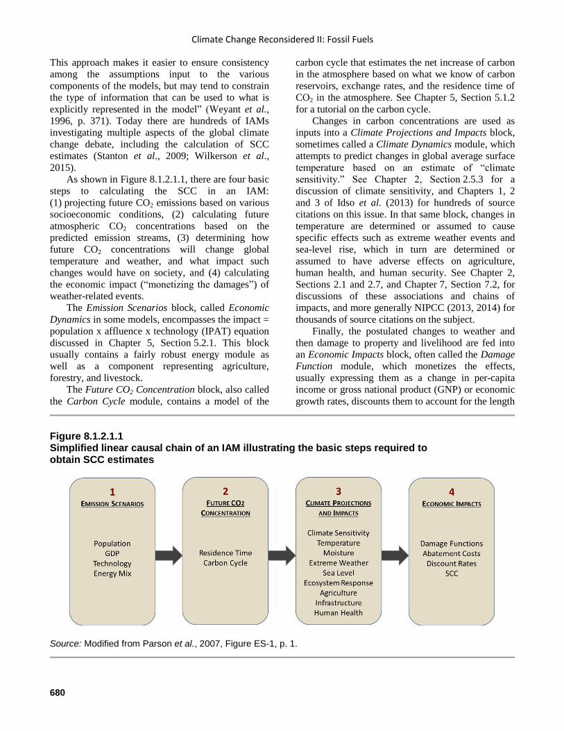
As shown in Figure 8.1.2.1.1, there are four basic

steps to calculating the SCC in an IAM:

(1) projecting future CO2 emissions based on various

socioeconomic conditions, (2) calculating future

atmospheric CO2 concentrations based on the

predicted emission streams, (3) determining how

future CO2 concentrations will change global

temperature and weather, and what impact such

changes would have on society, and (4) calculating

the economic impact (“monetizing the damages”) of

weather-related events.

The Emission Scenarios block, called Economic

Dynamics in some models, encompasses the impact =

population x affluence x technology (IPAT) equation

discussed in Chapter 5, Section 5.2.1. This block

usually contains a fairly robust energy module as

well as a component representing agriculture,

forestry, and livestock.

The Future CO2 Concentration block, also called

the Carbon Cycle module, contains a model of the

carbon cycle that estimates the net increase of carbon

in the atmosphere based on what we know of carbon

reservoirs, exchange rates, and the residence time of

CO2 in the atmosphere. See Chapter 5, Section 5.1.2

for a tutorial on the carbon cycle.

Changes in carbon concentrations are used as

inputs into a Climate Projections and Impacts block,

sometimes called a Climate Dynamics module, which

attempts to predict changes in global average surface

temperature based on an estimate of “climate

sensitivity.” See Chapter 2, Section 2.5.3 for a

discussion of climate sensitivity, and Chapters 1, 2

and 3 of Idso et al. (2013) for hundreds of source

citations on this issue. In that same block, changes in

temperature are determined or assumed to cause

specific effects such as extreme weather events and

sea-level rise, which in turn are determined or

assumed to have adverse effects on agriculture,

human health, and human security. See Chapter 2,

Sections 2.1 and 2.7, and Chapter 7, Section 7.2, for

discussions of these associations and chains of

impacts, and more generally NIPCC (2013, 2014) for

thousands of source citations on the subject.

Finally, the postulated changes to weather and

then damage to property and livelihood are fed into

an Economic Impacts block, often called the Damage

Function module, which monetizes the effects,

usually expressing them as a change in per-capita

income or gross national product (GNP) or economic

growth rates, discounts them to account for the length

Figure 8.1.2.1.1 Simplified linear causal chain of an IAM illustrating the basic steps required to obtain SCC estimates

Source: Modified from Parson et al., 2007, Figure ES-1, p. 1.

Cost-Benefit Analysis

681

of time that passes before the effects are experienced,

calculates the total (global) net social cost (or

benefit), divides it by the number of tons of carbon

dioxide emitted according to the Emission Scenarios

block, and produces a “social cost of carbon”

typically expressed in USD per metric ton of CO2-

equivalent greenhouse gases.

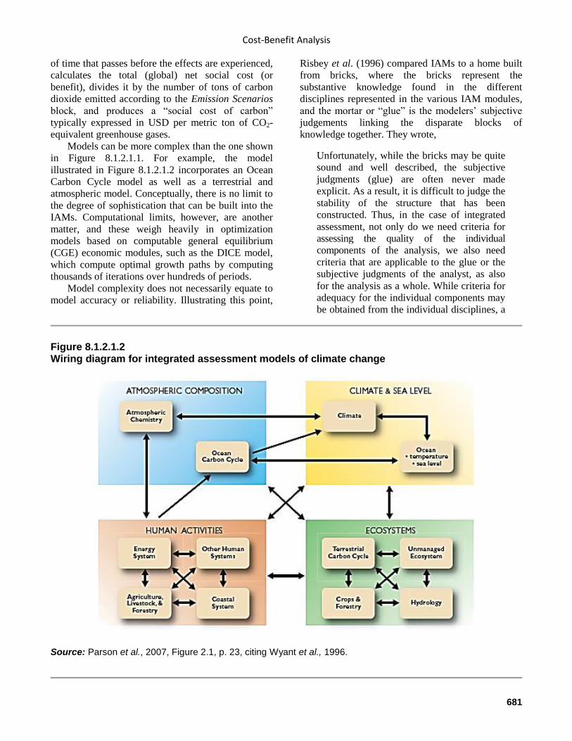
Models can be more complex than the one shown

in Figure 8.1.2.1.1. For example, the model

illustrated in Figure 8.1.2.1.2 incorporates an Ocean

Carbon Cycle model as well as a terrestrial and

atmospheric model. Conceptually, there is no limit to

the degree of sophistication that can be built into the

IAMs. Computational limits, however, are another

matter, and these weigh heavily in optimization

models based on computable general equilibrium

(CGE) economic modules, such as the DICE model,

which compute optimal growth paths by computing

thousands of iterations over hundreds of periods.

Model complexity does not necessarily equate to

model accuracy or reliability. Illustrating this point,

Risbey et al. (1996) compared IAMs to a home built

from bricks, where the bricks represent the

substantive knowledge found in the different

disciplines represented in the various IAM modules,

and the mortar or “glue” is the modelers’ subjective

judgements linking the disparate blocks of

knowledge together. They wrote,

Unfortunately, while the bricks may be quite

sound and well described, the subjective

judgments (glue) are often never made

explicit. As a result, it is difficult to judge the

stability of the structure that has been

constructed. Thus, in the case of integrated

assessment, not only do we need criteria for

assessing the quality of the individual

components of the analysis, we also need

criteria that are applicable to the glue or the

subjective judgments of the analyst, as also

for the analysis as a whole. While criteria for

adequacy for the individual components may

be obtained from the individual disciplines, a

Figure 8.1.2.1.2 Wiring diagram for integrated assessment models of climate change

Source: Parson et al., 2007, Figure 2.1, p. 23, citing Wyant et al., 1996.

Climate Change Reconsidered II: Fossil Fuels

682

similar situation does not exist for the ‘glue’

in the analysis (Risbey et al., 1996, p. 383).

Not only is the “glue” suspect in IAMs, but the

blocks themselves are also questionable. Major

module limitations include the simplicity of their

approach, using only one or two equations

associating aggregate damage to one climate variable

– in most cases temperature change – which does not

recognize interactions among different impacts. More

problems include the ability to capture only a limited

number of impacts and often omitting those impacts

that may be large but are difficult to quantify or show

high levels of uncertainty, and presenting damage in

terms of loss of income without recognizing capital

implications. A particularly difficult problem to solve

is the application of “willingness to pay” or “stated

preference” quantifications that frequently overstate

values relative to observed behavior, since people

responding to surveys face no real consequences in

terms of required payment for the good or service.

This positive “hypothetical bias” is widely noted and

discussed in economic literature (e.g., Murphy et al.,

2004; Vossler and Evans, 2009; Penn and Hu, 2018).

These and other weaknesses described below erode

confidence in the ability of IAMs to accurately

estimate the “social cost of carbon” in CBAs.

References

Murphy, J., et al. 2004. A meta-analysis of hypothetical

bias in stated preference valuation. Environmental and

Resource Economics 30 (3): 313–25.

NIPCC. 2013. Nongovernmental International Panel on

Climate Change. Climate Change Reconsidered II:

Physical Science. Chicago, IL: The Heartland Institute.

NIPCC 2014. Nongovernmental International Panel on

Climate Change. Climate Change Reconsidered II:

Biological Impacts. Chicago, IL: The Heartland Institute.

Parson, E., et al. 2007. Global-change scenarios: their

development and use. U.S. Department of Energy

Publications 7. Washington, DC.

Penn, J. and Hu, W. 2018. Understanding hypothetical

bias: an enhanced meta-analysis. American Journal of

Agricultural Economics 100 (4): 1186–1206.

Risbey, J., Kandlikar, M., and Patwardhan, A. 1996.

Assessing integrated assessments. Climatic Change 34:

369–95.

Stanton, E.A., Ackerman, F., and Kartha, S. 2009. Inside

the integrated assessment models: four issues in climate

economics. Climate and Development 1: 166–84.

Vossler, C. and Evans, M. 2009. Bridging the gap between

the field and the lab: environmental goods, policy maker

input, and consequentiality. Journal of Environmental

Economics and Management 58 (3): 338–45.

Weyant, J.P., et al. 1996. Chapter 10. Integrated

assessment of climate change: an overview and

comparison of approaches and results. In: Bruce, J.P., et al.

(Eds.) Climate Change 1995: Economic and Social

Dimensions of Climate Change. Intergovernmental Panel

on Climate Change. Cambridge, UK: Cambridge

University Press.

Wilkerson, J.T., et al. 2015. Comparison of integrated

assessment models: carbon price impacts on U.S. energy.

Energy Policy 76: 18–31.

8.1.2.2 Propagation of Error

IAMs suffer from propagation of error,

sometimes called cascading uncertainties,

whereby uncertainty in each stage of the

analysis compounds, resulting in wide

uncertainty bars surrounding any eventual

results.

“Propagation of error” is a term introduced in

Chapter 2, Section 2.1.1.3, used in statistics to refer

to how errors or uncertainty in one variable, due

perhaps to measurement limitations or confounding

factors, are compounded (or propagated) when that

variable becomes part of a function involving other

variables that are similarly uncertain. Error

propagation through sequential calculations is widely

used in the physical sciences to reveal the reliability

of an experimental result or of a calculation from

theory. As the number of variables or steps in a

function increases, uncertainties multiply until there

can be no confidence in the calculational outcomes.

In academic literature this is sometimes referred to as

“cascading uncertainties” or “uncertainty

explosions.”

Uncertainties in climate science, described in

Chapter 2, create major difficulties for IAMs.

Although considerable progress has been made in

climate science and in the understanding of how

human activity interacts with and impacts the

biosphere and economy, significant uncertainties

persist in each block or module of an IAM. As the

Cost-Benefit Analysis

683

model progresses through each of these phases,

uncertainties surrounding each variable in the chain

of computations are compounded one upon another,

creating a cascade of uncertainties that peaks upon

completion of the final calculation.

An interesting example of the uncertainty and

arbitrariness of damage functions can be shown in a

comparison conducted by Aldy et al. (2009) of the

results of IAM impact studies. They found there was

a significant amount of consistency among several

disparate studies of the economic impact of a 2.5°C

warming by 2100 of average global temperatures

compared to pre-industrial levels. Five models

predicted economic damages between 1% and 2% of

global GDP. However, although the gross damage

estimates were similar, there were huge differences in

the estimates of the sources of the damages within

each study. The similar results for the gross damage

estimates could have occurred by remarkable

coincidence. More likely, the modelers “tuned” their

models to arrive at total damage values they knew to

be in the range of what other researchers have

reported. This is an example of the “herding”

behavior documented in Chapter 2, Section 2.2.2.1,

and the “tuning” of climate models reported by

Voosen (2016) and Hourdin et al. (2017).

When confronted with the fact that their models

include only a limited number of sectors of the

economy, the modelers typically argue any

unrepresented sectors would result in even greater

damage assessment if included. For example, the

IPCC says “Different studies include different

aspects of the impacts of climate change, but no

estimate is complete; most experts speculate that

excluded impacts are on balance negative” (IPCC,

2014, p. 690). However, little evidence is presented

to support these claims. In contrast, as shown in

previous chapters of this volume, the opposite is

more likely to be true. Tunnel vision prevents

bureaucracies from searching for evidence that might

seem to lower the risk of the problem they are

responsible for solving, so the “excluded impacts”

are likely to be exculpatory rather than reinforce the

government’s theory. Publication bias (the tendency

of academic journals to publish research that finds

associations and not to publish those that do not)

means more research is likely to reveal that

relationships between climate change and alleged

impacts is weaker than currently thought.

IAMs increasingly address the issue of

uncertainty by including probability distributions – a

range of values around a norm – of the parameters to

explicitly address the issue of uncertainty. While this

serves to acknowledge that we have no real scientific

evidence to support one value over another, their use

introduces another bias into IAM results. Since the

structure of the damage function is made up of

quadratic equations, the results of using probability

distributions of equation parameters results in so-

called “fat tail” impacts that are larger for higher

temperature increases than for lower increases.

Multiplying a series of upper-bound estimates results

in a phenomenon called “cascading conservatism”

(Council of Economic Advisors, 2004, p. 179) or

what Belzer (2012, p. 13) calls “cascading bias,”

leading to risk assessments that are orders of

magnitude higher than what observational data

suggest.

Many experts have concluded the uncertainty

problem affecting IAMs makes them too unreliable to

form the basis of public policy decisions. Payne

(2014) noted “the activist policy [of reducing CO2

emissions] depends on a teetering chain of

improbabilities” and represents “an extensive chain

of assumptions, every one of which has to be true in

order for carbon-dioxide-limiting policies to be

justified.” Pindyck wrote in the Journal of Economic

Literature in 2013,

[IAMs] have crucial flaws that make them

close to useless as tools for policy analysis:

certain inputs (e.g., the discount rate) are

arbitrary, but have huge effects on the SCC

estimates the models produce; the models’

descriptions of the impact of climate change

are completely ad hoc, with no theoretical or

empirical foundation; and the models can tell

us nothing about the most important driver of

the SCC, the possibility of a catastrophic

climate outcome. IAM-based analyses of

climate policy create a perception of

knowledge and precision, but that perception

is illusory and misleading (Pindyck, 2013a,

abstract).

Writing that same year in the Review of

Environmental Economics and Policy, Pindyck

(2013b, p. 6) also observed:

IAM damage functions are completely made

up, with no theoretical or empirical

foundation. They simply reflect common

beliefs (which might be wrong) regarding the

impact of 2°C or 3°C of warming, and can

tell us nothing about what might happen if

the temperature increases by 5°C or more.

Climate Change Reconsidered II: Fossil Fuels

684

And yet those damage functions are taken

seriously when IAMs are used to analyze

climate policy.

Harvard University’s Martin Weitzman (2015,

pp. 145–6) has commented,

[D]isconcertingly large uncertainties are

everywhere, including the most challenging

kinds of deep structural uncertainties. The

climate change problem unfolds over

centuries and millennia, a long

intergenerational human time frame that most

people are entirely unaccustomed to thinking

about. With such long time frames,

discounting becomes ultra-decisive for BCA,

and there is much debate and confusion about

which long-run discount rate should be

chosen.

According to Tapia Granados and Carpintero

(2013, p. 40), “The lack of robustness of results of

different IAMs indicates the limitations of the

neoclassical approach, which constitutes the

theoretical base of most IAMs; the variety of so-

called ad hoc assumptions (often qualified as ‘heroic’

by their own authors), and the controversial nature of

the methods to estimate the monetary value of non-

market costs and benefits (mortality, morbidity,

damage to ecosystems, etc.). These features explain

why many contributions of this type of

macroeconomics-oriented IAMs have been criticized

for their dubious political usefulness and limited

scientific soundness.”

Tapia Granados and Carpintero then presented

several important shortcomings of IAMs, most of

which have been discussed previously: (1) a lack of

transparency to explain and justify the assumptions

behind the estimates, (2) questionable treatment of

uncertainty and discounting of the future, (3)

assumption of perfect substitutability between

manufactured capital and “natural” capital in the

production of goods and services, and (4) problems in

the way IAMs estimate monetary costs of non-market

effects, which can lead to skepticism about policies

based on the results of the models. In another blunt

assessment, Ackerman et al. (2009, pp. 131–2) wrote:

[P]olicy makers and scientists should be

skeptical of efforts by economists to specify

optimal policy paths using the current

generation of IAMs. These models do not

embody the state of the art in the economic

theory of uncertainty, and the foundations of

the IAMs are much shakier than the general

circulation models that represent our best

current understanding of physical climate

processes. Not only do the IAMs entail an

implicit philosophical stance that is highly

contestable, they suffer from technical

deficiencies that are widely recognized

within economics.

Even the latest contributors to the IPCC’s

assessment reports agree. According to the Working

Group II contribution to Chapter 10 of the Fifth

Assessment Report (AR5), “Uncertainty in SCC

estimates is high due to the uncertainty in underlying

total damage estimates (see Section 10.9.2),

uncertainty about future emissions, future climate

change, future vulnerability and future valuation. The

spread in estimates is also high due to disagreement

regarding the appropriate framework for aggregating

impacts over time (discounting), regions (equity

weighing), and states of the world (risk aversion).”

As the result of such uncertainties, they say,

Quantitative analyses have shown that SCC

estimates can vary by at least approximately

two times depending on assumptions about

future demographic conditions (Interagency

Working Group on the Social Cost of

Carbon, 2010), at least approximately three

times owing to the incorporation of

uncertainty (Kopp et al., 2012), and at least

approximately four times owing to

differences in discounting (Tol, 2011) or

alternative damage functions (Ackerman and

Stanton, 2012) (IPCC, 2014, p. 691).

According to the IPCC, “In sum, estimates of the

aggregate economic impact of climate change are

relatively small but with a large downside risk.

Estimates of the incremental damage per tonne of

CO2 emitted vary by two orders of magnitude, with

the assumed discount rate the main driver of the

differences between estimates. The literature on the

impact of climate and climate change on economic

growth and development has yet to reach firm

conclusions. There is agreement that climate change

would slow economic growth, by a little according to

some studies and by a lot according to other studies.

Different economies will be affected differently.

Some studies suggest that climate change may trap

more people in poverty” (Ibid., p. 692–693, italics

added).

Cost-Benefit Analysis

685

For the foreseeable future, IAM analyses will be

saddled with the fact that the degree of uncertainty

within the various computational stages is immense –

especially when the most significant input is

subjective (i.e., the discount rate). For all practical

purposes the errors inherent to IAMs render their use

as policy tools highly questionable, if not

irresponsible. They are simply not capable of

providing realistic estimates of the SCC, nor can they

justify GHG emission reduction policies.

References

Ackerman, F., et al. 2009. Limitations of integrated

assessment models of climate change. Climatic Change

95: 297–315.

Ackerman, F. and Stanton, E.A. 2012. Climate risks and

climate prices: revisiting the social cost of carbon.

Economics: The Open-Access, Open-Assessment E-

Journal 6 (10).

Aldy, J.E., et al. 2009. Designing climate mitigation

policy. RFF DP 08-16. Washington, DC: Resources for the

Future. May.

Belzer, R. 2012. Risk Assessment, Safety Assessment, and

the Estimation of Regulatory Benefits. Mercatus Research.

Washington, DC: Mercatus Center.

Council of Economic Advisors. 2004. Economic Report of

the President. Washington, DC: Government Printing

Office.

Hourdin, F., et al. 2017. The art and science of climate

model tuning. Bulletin of the American Meteorological

Society 98 (3): 589–602.

IPCC. 2001. Intergovernmental Panel on Climate Change.

Climate Change 2001: Impacts, Adaptation and

Vulnerability. Contribution of Working Group II to the

Third Assessment Report of the Intergovernmental Panel

on Climate Change. New York, NY: Cambridge

University Press.

IPCC. 2014. Intergovernmental Panel on Climate Change.

Climate Change 2014: Impacts, Adaptation, and

Vulnerability. Part A: Global and Sectoral Aspects.

Contribution of Working Group II to the Fifth Assessment

Report of the Intergovernmental Panel on Climate Change.

New York, NY: Cambridge University Press.

IWG. 2010. Interagency Working Group on the Social

Cost of Carbon. Social Cost of Carbon for Regulatory

Impact Analysis under Executive Order 12866.

Washington, DC. February.

Kopp, R.E., Golub, A., Keohane, N.O., and Onda, C.

2012: The influence of the specification of climate change

damages on the social cost of carbon. Economics: The

Open-Access, Open-Assessment E-Journal 6: 2012–3.

Payne, J.L. 2014. The real case against activist global

warming policy. The Independent Review 19: 265–70.

Pindyck, R.S. 2013a. Climate change policy: what do the

models tell us? Journal of Economic Literature 51: 860–

72.

Pindyck, R.S. 2013b. The climate policy dilemma. Review

of Environmental Economics and Policy 7: 219–37.

Tapia Granados, J.A. and Carpintero, O. 2013. Dynamics

and economic aspects of climate change. In: Kang, M.S.

and Banga, S.S. (Eds.) Combating Climate Change: An

Agricultural Perspective. Boca Raton, FL: CRC Press.

Tol, R.S.J. 2011: The social cost of carbon. Annual Review

of Resource Economics 3: 419–43.

Voosen, P. 2016. Climate scientists open up their black

boxes to scrutiny. Science 354: 401–2.

Weitzman, M.L. 2015. A review of William Nordhaus’

“The climate casino: risk, uncertainty, and economics for a

warming world. Review of Environmental Economics and

Policy 9: 145–56.

8.1.3 IWG Reports

The widely cited “social cost of carbon”

calculations produced during the Obama

administration by the Interagency Working

Group on the Social Cost of Carbon have

been withdrawn and are not reliable guides

for policymakers.

On March 28, 2017, President Donald Trump issued

an executive order ending the U.S. government’s

endorsement of estimates of the “social cost of

carbon” (SCC) (Trump, 2017). The executive order,

which also rescinded other legacies of the Obama

administration’s environmental agenda, read in part:

Section 5. Review of Estimates of the Social

Cost of Carbon, Nitrous Oxide, and Methane

for Regulatory Impact Analysis.

(a) In order to ensure sound regulatory

decision making, it is essential that agencies

use estimates of costs and benefits in their

regulatory analyses that are based on the best

available science and economics.

Climate Change Reconsidered II: Fossil Fuels

686

(b) The Interagency Working Group on the

Social Cost of Greenhouse Gases (IWG),

which was convened by the Council of

Economic Advisers and the OMB Director,

shall be disbanded, and the following

documents issued by the IWG shall be

withdrawn as no longer representative of

governmental policy:

(i) Technical Support Document: Social Cost

of Carbon for Regulatory Impact Analysis

Under Executive Order 12866 (February

2010);

(ii) Technical Update of the Social Cost of

Carbon for Regulatory Impact Analysis (May

2013);

(iii) Technical Update of the Social Cost of

Carbon for Regulatory Impact Analysis

(November 2013);

(iv) Technical Update of the Social Cost of

Carbon for Regulatory Impact Analysis (July

2015);

(v) Addendum to the Technical Support

Document for Social Cost of Carbon:

Application of the Methodology to Estimate

the Social Cost of Methane and the Social

Cost of Nitrous Oxide (August 2016); and

(vi) Technical Update of the Social Cost of

Carbon for Regulatory Impact Analysis

(August 2016).

(c) Effective immediately, when monetizing

the value of changes in greenhouse gas

emissions resulting from regulations,

including with respect to the consideration of

domestic versus international impacts and the

consideration of appropriate discount rates,

agencies shall ensure, to the extent permitted

by law, that any such estimates are consistent

with the guidance contained in OMB

Circular A-4 of September 17, 2003

(Regulatory Analysis), which was issued

after peer review and public comment and

has been widely accepted for more than a

decade as embodying the best practices for

conducting regulatory cost-benefit analysis

(Trump, 2017).

It is not unusual for a president to rescind his

predecessor’s executive orders, and Trump’s

predecessor relied heavily on executive orders to

implement his anti-fossil-fuel agenda. Disbanding the

Interagency Working Group (IWG) sent a clear

signal that the president did not want to see the

“social cost of carbon” concept kept alive by agency

bureaucrats.

The IWG was comprised of representatives from

12 federal agencies brought together specifically to

come up with a number – the alleged damages due to

climate change caused by each ton of CO2 emitted by

the use of fossil fuels – that could be used to support

President Barack Obama’s war on fossil fuels (IER,

2014, p. 2). It was an example of the “seeing like a

state” phenomenon reported by Scott (1998) and

discussed in Chapter 1, Section 1.3.4, when

government agencies succumb to pressure to find

what they believe their overseers want them to find.

IWG utilized experts from numerous agencies who

explored technical literature in relevant fields,

discussed key model inputs and assumptions,

considered public comments, and then duly produced

some stylized facts to meet the government’s needs.

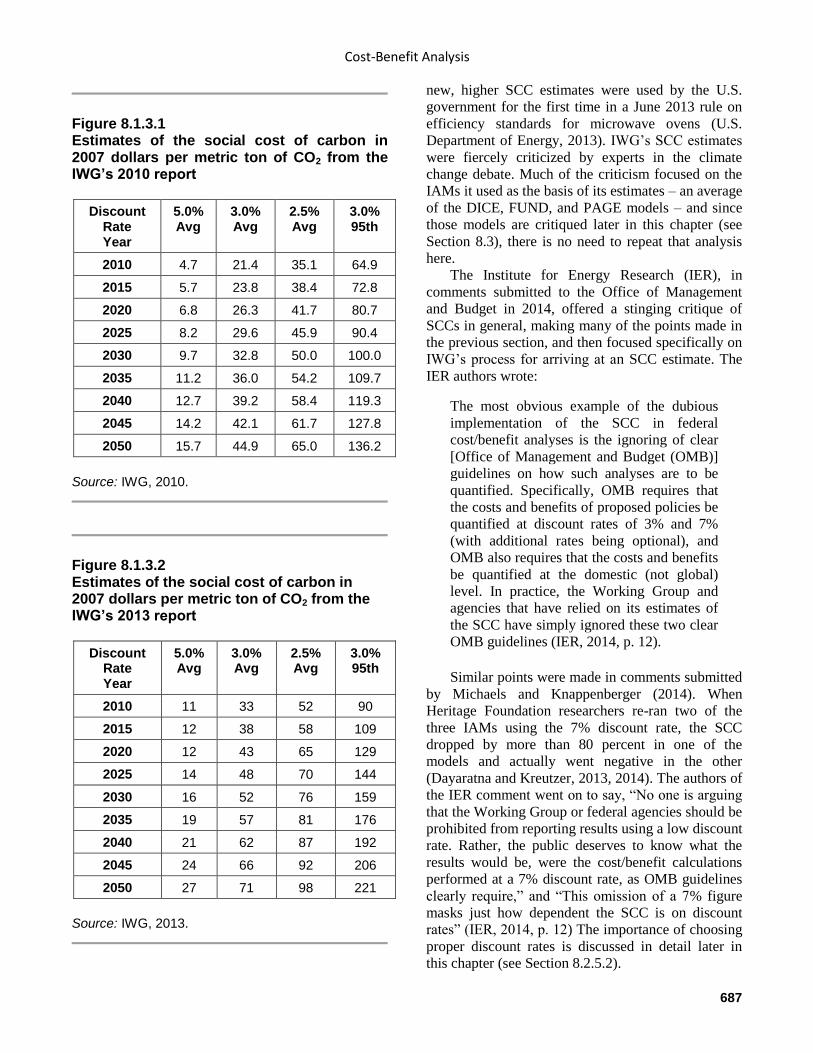
The first IWG report, issued in 2010, put the

social cost of carbon in 2010 at between $4.70 and

$35.10 per metric ton of CO2, depending on the

discount rate used (5% for the lower estimate and

2.5% for the higher estimate) (IWG, 2010). The

numbers were based on the average SCC calculated

by three IAMs (DICE, PAGE, and FUND) and three

discount rates (2.5%, 3%, and 5%). A fourth value

was calculated as the 95th percentile SCC estimate

across all three models at a 3% discount rate and was

included to characterize higher-than-expected

impacts from temperature change in the tails of the

SCC distribution. See Figure 8.1.3.1.

New versions of the three IAMs prompted IWG to

recalculate and publish revised SCC estimates in

2013, shown in Figure 8.1.3.2 below (IWG, 2013). In

this follow-up exercise, IWG did not revisit other

methodological decisions so no changes were made

to the discount rate, reference case socioeconomic

and emission scenarios, or equilibrium climate

sensitivity. Changes in the way damages are modeled

were confined to those that had been incorporated

into the latest versions of the models by the

developers themselves and reported in the peer-

reviewed literature.

The IWG’s new estimates for the SCC in 2010

ranged from $11 to $52 per metric ton of CO2, once

again depending on the discount rate used,

considerably higher than its previous estimate. The

Cost-Benefit Analysis

687

Figure 8.1.3.1 Estimates of the social cost of carbon in 2007 dollars per metric ton of CO2 from the IWG’s 2010 report

Discount Rate Year

5.0% Avg

3.0% Avg

2.5% Avg

3.0% 95th

2010 4.7 21.4 35.1 64.9

2015 5.7 23.8 38.4 72.8

2020 6.8 26.3 41.7 80.7

2025 8.2 29.6 45.9 90.4

2030 9.7 32.8 50.0 100.0

2035 11.2 36.0 54.2 109.7

2040 12.7 39.2 58.4 119.3

2045 14.2 42.1 61.7 127.8

2050 15.7 44.9 65.0 136.2

Source: IWG, 2010.

Figure 8.1.3.2 Estimates of the social cost of carbon in 2007 dollars per metric ton of CO2 from the IWG’s 2013 report

Discount Rate Year

5.0% Avg

3.0% Avg

2.5% Avg

3.0% 95th

2010 11 33 52 90

2015 12 38 58 109

2020 12 43 65 129

2025 14 48 70 144

2030 16 52 76 159

2035 19 57 81 176

2040 21 62 87 192

2045 24 66 92 206

2050 27 71 98 221

Source: IWG, 2013.

new, higher SCC estimates were used by the U.S.

government for the first time in a June 2013 rule on

efficiency standards for microwave ovens (U.S.

Department of Energy, 2013). IWG’s SCC estimates

were fiercely criticized by experts in the climate

change debate. Much of the criticism focused on the

IAMs it used as the basis of its estimates – an average

of the DICE, FUND, and PAGE models – and since

those models are critiqued later in this chapter (see

Section 8.3), there is no need to repeat that analysis

here.

The Institute for Energy Research (IER), in

comments submitted to the Office of Management

and Budget in 2014, offered a stinging critique of

SCCs in general, making many of the points made in

the previous section, and then focused specifically on

IWG’s process for arriving at an SCC estimate. The

IER authors wrote:

The most obvious example of the dubious

implementation of the SCC in federal

cost/benefit analyses is the ignoring of clear

[Office of Management and Budget (OMB)]

guidelines on how such analyses are to be

quantified. Specifically, OMB requires that

the costs and benefits of proposed policies be

quantified at discount rates of 3% and 7%

(with additional rates being optional), and

OMB also requires that the costs and benefits

be quantified at the domestic (not global)

level. In practice, the Working Group and

agencies that have relied on its estimates of

the SCC have simply ignored these two clear

OMB guidelines (IER, 2014, p. 12).

Similar points were made in comments submitted

by Michaels and Knappenberger (2014). When

Heritage Foundation researchers re-ran two of the

three IAMs using the 7% discount rate, the SCC

dropped by more than 80 percent in one of the

models and actually went negative in the other

(Dayaratna and Kreutzer, 2013, 2014). The authors of

the IER comment went on to say, “No one is arguing

that the Working Group or federal agencies should be

prohibited from reporting results using a low discount

rate. Rather, the public deserves to know what the

results would be, were the cost/benefit calculations

performed at a 7% discount rate, as OMB guidelines

clearly require,” and “This omission of a 7% figure

masks just how dependent the SCC is on discount

rates” (IER, 2014, p. 12) The importance of choosing

proper discount rates is discussed in detail later in

this chapter (see Section 8.2.5.2).

Climate Change Reconsidered II: Fossil Fuels

688

The IWG’s decision to include in its cost-benefit

analysis estimates of the global costs (and

presumably benefits) of climate change reflected the

fact that the three IAMs it chose to rely on attempt to

find a global cost rather than a cost specific to the

United States. But not only does this violate the

purpose of CBA as set forth in national policy

guidelines, it also produces false results by

disregarding the “leakage” problem reported in

Chapter 1, Section 1.2.10, which found reducing

emissions in the United States by 10 metric tons

could cause emissions by other countries to increase

between 1.2 and 13 tons (Brown, 1999; Babiker,

2005).

A net reduction of 10 tons assuming the lower of

the two estimates would require an emissions

reduction by the United States of 11.4 tons, so the

IWG estimate of the SCC is too low. The second

estimate means no reductions by the United States,

no matter how high, will lead to a net reduction in

global emissions since emissions in other countries

rise faster than reductions in the United States. In

choosing to use a global estimate of damages in its

SCC, the IWG disregarded an extensive body of

literature on leakage rates by industry, by type of

program, and by country (Fischer et al., 2010).

Finally, the IER researchers also observe that

“According to Cass Sunstein, the man who convened

the SCC Working Group, ‘Neither the 2010 TSD

[Technical Support Document] nor the 2013 update

was subject to peer review in advance, though an

interim version was subject to public comment in

2009’ [Sunstein, 2013]. This is a direct violation of

the administration’s stance on ‘Transparency and

Open Government’ [Obama, 2009]” (IER, 2014, p.

19).

For all these reasons, the Trump administration

was right to withdraw the social cost of carbon

calculations produced during the Obama

administration by the Interagency Working Group on

the Social Cost of Carbon.

References

Babiker, M.H. 2005. Climate change policy, market

structure, and carbon leakage. Journal of International

Economics 65: 421.

Brown, S.P.A. 1999. Global Warming Policy: Some

Economic Implications. Policy Report #224. Dallas, TX:

National Center for Policy Analysis.

Dayaratna, K. and Kreutzer, D. 2013. Loaded DICE: an

EPA model not ready for the big game. Backgrounder No.

2860. Washington, DC: The Heritage Foundation.

November 21.

Dayaratna, K. and Kreutzer, D. 2014. Unfounded FUND:

yet another EPA model not ready for the big game.

Backgrounder No. 2897. Washington, DC: The Heritage

foundation. April 29.

Fischer, C., Moore, E., Morgenstern, R., and Arimura, T.

2010. Carbon Policies, Competitiveness, and Emissions

Leakage: An International Perspective. Washington, DC:

Resources for the Future.

IER. 2014. Institute for Energy Research. Comment on

technical support document: technical update of the social

cost of carbon for regulatory impact analysis under

executive order no. 12866. February 24. IWG. 2010. Interagency Working Group on the Social

Cost of Carbon. Social Cost of Carbon for Regulatory

Impact Analysis under Executive Order 12866.

Washington, DC. February.

IWG. 2013. Interagency Working Group on the Social

Cost of Carbon. Technical Update of the Social Cost of

Carbon for Regulatory Impact Analysis Under Executive

Order 12866. Washington, DC. November.

Michaels, P. and Knappenberger, P. 2014. Comment for

Cato Institute on “Office of Management and Budget’s

request for comments on the technical support document

entitled technical update of the social cost of carbon for

regulatory impact analysis under executive order 12866.”

January 27.

Obama, B. 2009. Memorandum for the heads of executive

departments and agencies on transparency and open

government. Washington, DC: White House. January 21.

Scott, J.C. 1998. Seeing Like a State: How Certain

Schemes to Improve the Human Condition Have Failed.

New Haven, CT: Yale University Press.

Sunstein, C.R. 2013. On not revisiting official discount

rates: institutional inertia and the social cost of carbon.

Regulatory Policy Program Working Paper RPP-2013-21.

Cambridge, MA: Mossavar-Rahmani Center for Business

and Government, Harvard Kennedy School, Harvard

University.

Trump, D. 2017. Presidential Executive Order on

Promoting Energy Independence and Economic Growth.

March 28.

U.S. Department of Energy. 2013. Energy conservation

program: energy conservation standards for standby mode

Cost-Benefit Analysis

689

and off mode for microwave ovens. Federal Register 78

(116): 10 CFR Parts 429 and 430.

8.1.4 The Stern Review

The widely cited “Stern Review” was an

important early attempt to apply cost-benefit

analysis to climate change. Its its authors

focused on worst-case scenarios and failed to

report profound uncertainties.

The Economics of Climate Change: The Stern Review

was prepared for the British government by Nicholas

Stern, professor of economics and government at the

London School of Economics, released in October

2006, and published by Cambridge University Press

in 2007 (Stern et al., 2007). Commonly known as the

Stern Review, it claimed “using the results from

formal economic models, the Review estimates that if

we don’t act, the overall costs and risks of climate

change will be equivalent to losing at least 5% of

global GDP each year, now and forever. If a wider

range of risks and impacts is taken into account, the

estimates of damage could rise to 20% of GDP or

more.”

The Stern Review’s findings were markedly

different from prior works on the subject and thus led

to questions as to how and why its authors came to

such a radically different conclusion. It did not take

long for researchers to determine the disparity and

the report was quickly refuted (Byatt et al., 2006;

Mendelsohn, 2006; Nordhaus, 2006; Tol and Yohe,

2006). Nevertheless, the report was heralded

throughout the policy world and continues to be

frequently cited as justification for enacting CO2

emission reduction policies. Following are some key

shortcomings of the report.

Uncertainty. Uncertainties all along the chain of

calculations are poorly expressed or not

acknowledged at all, creating the appearance of a

specific and certain finding (such as the numbers

cited above) even though its conclusions could be off

by an order of magnitude or even reverse sign. This

sort of rhetoric is tolerated in the “gray literature” –

policy research and commentary that is not peer-

reviewed – but it should not then be presented as an

authoritative scientific report.

Emission Scenarios. The Stern Review

uncritically endorses the IPCC’s future emissions

scenarios, which have been widely criticized as

problematic and based on flawed economic analyses

to which no probabilities have been assigned

(Henderson, 2005). As an example, the Stern Review

considers only one baseline of demographic change

over the next two centuries, which assumes rapid

population growth in lower latitudes. Further, the

scenario assumes an anemic growth in per-capita

income of only 1.3% per year instead of recent

growth rates of approximately 3%. This blend of

assumptions creates a future full of billions of poor

people living in regions deemed most sensitive to

warming. Had the Stern Review assumed economic

growth to continue at just 2%, and if population

growth rates continued to slow, there would actually

be a reduction in the poorest and most vulnerable

rural populations in these lower latitudes.

Climate Impacts. The Stern Review consistently

exaggerates the potential impacts of climate change,

giving much more weight and credence to worst-case

future climate scenarios. The report assumes

powerful positive feedbacks will cause temperatures

to increase more rapidly than previously thought,

especially throughout the twenty-second century. The

central assumption is temperatures might rise 2° to

5°C by 2100, and then by another 2°C by 2200. But

the report also raises the possibility warming might

be as high as 10° to 11°C by 2100, in which event the

global cost is estimated to be as high as 5% to 20% of

GDP.

Much of the economic damages are expected to

result from increasing extreme weather events, which

gain in magnitude and frequency and time in the

Stern Review. Observational evidence, in contrast,

shows no conclusive relationship between extreme

weather events and global warming, with much of the

literature suggestive that such events will decline as

temperatures warm (see Chapter 2 and references in

NIPCC, 2013, Chapter 7). Estimated annual climate-

related damages in the Stern Review amount to only

0.2% of GDP at present but rise to 5% of GDP in

2200. This translates to around $70 billion in

damages in 2000 to a staggering $23 trillion per year

by 2200. There is no evidence to suggest climate

impacts could possibly reach this height.

Discount Rate. The Stern Review utilized an

extremely low value for the discount rate, just 1.4%.

As discussed in some detail in Section 8.2.5.2, the

application of such a low value will inherently

produce a very high SCC (one dollar of damage in

2200 is worth six cents in 2000 if discounted at 1.4%,

but worth only 0.03 cents if discounted at 4%). The

authors of the Stern Review argue for using the 1.4%

value, which is only 0.1% above the rate of growth of

consumption in their analysis, saying it is “ethically

proper” – they consider using a higher discount rate

Climate Change Reconsidered II: Fossil Fuels

690

to be unfair to future generations. In fact, using a low

discount rate to justify draconian reductions on CO2

emissions today would reduce the welfare of all

generations by slowing economic growth today and

for decades to come. Further, by using a low discount

rate, the Stern Review placed too much near-term

significance on events that may occur only far into

the future.

Another problem concerning the discount rate

was pointed out by Mendelsohn (2006, p. 43), who

wrote

Despite arguing for the low discount rate in

the impact analysis, the report does not use it

when evaluating the cost of mitigation. To be

consistent, the opportunity cost of investing

in mitigation must also be valued using the

same discount rate as was used to determine

the cost of climate change. Because investing

in mitigation substitutes for investing in other

activities that can earn the market rate of

interest, society loses the income that it could

have gained from other valuable projects.

Assuming that we use the historic rate of

return of 4% (that the mitigation program

does not drive up interest rates), the value of

$1 of abatement is $2.9 when evaluated at a

discount rate of 1.4%. The mitigation costs

reported in the study need to be multiplied by

a factor of three to be consistent with how the

damages are calculated.

No Adaptation. Despite discussing the

importance of human adaptation to climate change at

various points in the report, the influence of

adaptation on welfare damages is not taken into

account. As Mendelsohn (2006, p. 44) once again

critiqued: “[T]he report’s estimates of flood damage

costs from earlier spring thaws do not consider the

probability that people will build dams to control the

flooding. Farmers are envisioned as continuing to

grow crops that are ill suited for new climates. People

do not adjust to the warmer temperatures they

experience year after year, and they thus die from

heat stroke. Protective structures are not built along

the coasts to stop rising sea levels from flooding

cities. No public health measures are taken to stop

infectious diseases from spreading.” The result is that

“compared to studies that include adaptation, the

[Stern] report overestimates damages by more than

an order of magnitude” (Ibid.).

Emission Abatement. The Stern Review concedes

a present-day high cost of abatement. To reach the

stabilization goal of 550 ppm, which corresponds to a

two-thirds reduction in emissions by 2050, a carbon

tax on the order of $168 per ton would need to be

implemented, amounting to a rough estimate of $8.9

trillion per year, which is 6.5% of GDP, or a

displaced investment worth about 20% of GDP. The

Stern Review reassures its readers these costs will be

reduced over time by technological advancements

that will drive the costs to only 3% of GDP in 2020

and 1% in 2050. But the costs of technologies do not

always fall over time.

Mendelsohn (2006, p. 46) wrote, “Many

technologies have been abandoned precisely because

their costs have not fallen. Moreover, one must be

careful projecting how far costs will fall because one

will eventually exhaust all the possible improvements

that can be made. One of the critical linchpins of the

Stern Report is that technical change will drive down

the cost of abatement six-fold by 2050.”

Carbon recapture remains a costly, unproven

technology and there are multiple problems with

renewable technology (see Chapter 3). To meet the

Stern Review’s goals, Mendelsohn notes, an area

covering some 5 million to 10 million hectares of

land would be needed for solar panels (in sunny

locations), 33 million hectares would be needed to

install two million additional wind turbines, and a

whopping 500 million additional hectares of land

would be needed to increase energy production from

biofuels (Mendelsohn, 2006, p. 45). And, despite the

increased pressure these actions would place on land,

the Stern Review assumes they would have no impact

on the price of land, nor on the industries from which

the land presumably would be taken (agriculture,

timber, and tourism).

Economic Impact. Because of its errors in

emission scenarios, estimates of climate impact, use

of improper discount rates, and failure to consider

adaptation, the Stern Review’s claim that unabated

global warming would produce large negative

economic impacts “now and forever” is not credible.

Unlike most other studies, the Stern Review attempts

to account for non-market (i.e., environmental)

impacts as well as the risk of catastrophe (see, e.g.,

Freeman and Guzman, 2009, p. 127). Tol observes,

“[The Stern Review’s] impact estimates are

pessimistic even when compared to other studies in

the gray literature and other estimates that use low

discount rates” (Tol, 2008, p. 9).

Goklany (2009) used the Stern Review’s four

emission scenarios (taken from the IPCC’s Third

Assessment Report (TAR)) and its inflated estimates

of the damages caused by global warming (expressed

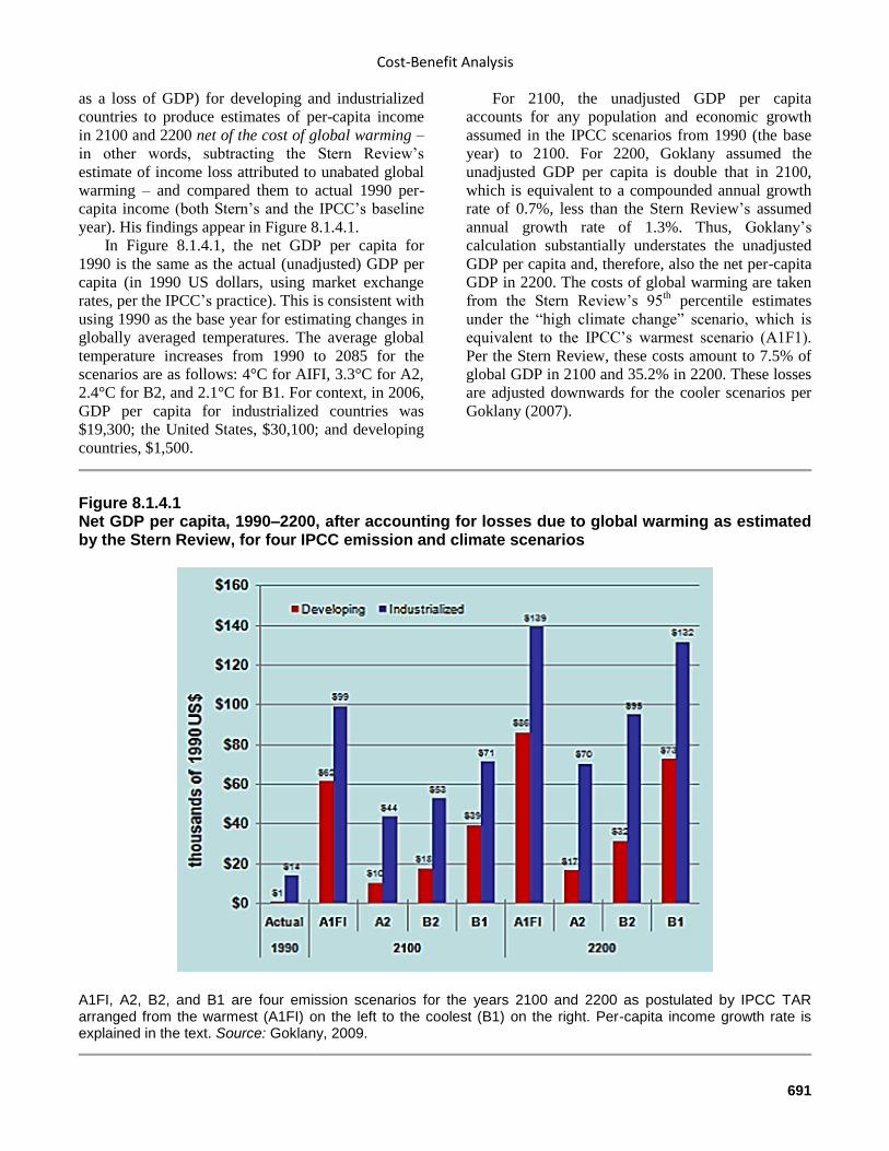
Cost-Benefit Analysis

691

as a loss of GDP) for developing and industrialized

countries to produce estimates of per-capita income

in 2100 and 2200 net of the cost of global warming –

in other words, subtracting the Stern Review’s

estimate of income loss attributed to unabated global

warming – and compared them to actual 1990 per-

capita income (both Stern’s and the IPCC’s baseline

year). His findings appear in Figure 8.1.4.1.

In Figure 8.1.4.1, the net GDP per capita for

1990 is the same as the actual (unadjusted) GDP per

capita (in 1990 US dollars, using market exchange

rates, per the IPCC’s practice). This is consistent with

using 1990 as the base year for estimating changes in

globally averaged temperatures. The average global

temperature increases from 1990 to 2085 for the

scenarios are as follows: 4°C for AIFI, 3.3°C for A2,

2.4°C for B2, and 2.1°C for B1. For context, in 2006,

GDP per capita for industrialized countries was

$19,300; the United States, $30,100; and developing

countries, $1,500.

For 2100, the unadjusted GDP per capita

accounts for any population and economic growth

assumed in the IPCC scenarios from 1990 (the base

year) to 2100. For 2200, Goklany assumed the

unadjusted GDP per capita is double that in 2100,

which is equivalent to a compounded annual growth

rate of 0.7%, less than the Stern Review’s assumed

annual growth rate of 1.3%. Thus, Goklany’s

calculation substantially understates the unadjusted

GDP per capita and, therefore, also the net per-capita

GDP in 2200. The costs of global warming are taken

from the Stern Review’s 95th percentile estimates

under the “high climate change” scenario, which is

equivalent to the IPCC’s warmest scenario (A1F1).

Per the Stern Review, these costs amount to 7.5% of

global GDP in 2100 and 35.2% in 2200. These losses

are adjusted downwards for the cooler scenarios per

Goklany (2007).

Figure 8.1.4.1 Net GDP per capita, 1990–2200, after accounting for losses due to global warming as estimated by the Stern Review, for four IPCC emission and climate scenarios

A1FI, A2, B2, and B1 are four emission scenarios for the years 2100 and 2200 as postulated by IPCC TAR arranged from the warmest (A1FI) on the left to the coolest (B1) on the right. Per-capita income growth rate is explained in the text. Source: Goklany, 2009.

Climate Change Reconsidered II: Fossil Fuels

692

Figure 8.1.4.1 shows that even accepting the

Stern Review’s unrealistic assumptions and highest

damage estimates, and despite assuming an economic

growth rate in the absence of global warming that is

less than the already low rate assumed by the Stern

Report, for populations living in countries currently

classified as “developing,” net GDP per capita (after

accounting for global warming) will be 11 to 65

times higher in 2100 than it was in the base year. It

will be even higher (18 to 95 times) in 2200.

Goklany’s calculation also found that

industrialized countries will have net GDP per capita

three to seven times higher in 2100 than in 1990. In

2200 it will be five to 10 times higher. Net GDP per

capita in today’s developing countries will be higher

in 2200 than it was in industrialized countries in the

base year (1990) under all scenarios, despite any

global warming. That is, regardless of any global

warming, populations living in today’s developing

countries will be far better off in the future than

people currently inhabiting today’s industrialized

countries. This is also true for 2100 for all but the

“poorest” (A2) scenario.

Under the warmest scenario (A1FI), the scenario

that prompts much of the apocalyptic warnings about

global warming, net GDP per capita of inhabitants of

developing countries in 2100 ($61,500) will be

double that of the United States in 2006 ($30,100),

and almost triple in 2200 ($86,200 versus $30,100).

(All dollar estimates are in 1990 US dollars.)

In other words, if the Stern Review’s pessimistic

scenario were to come about, people everywhere –

even in developing countries – would be wealthy by

today’s standards, and their ability to cope with and

adapt to climate change will be correspondingly

higher.

* * *

In conclusion, at the time of its publication in

2007 the Stern Review was a serious attempt to

estimate the social costs and benefits of climate

change. Written by a distinguished author (and team

of assistants), it was and still is accepted as being at

least close to the mark by many policymakers and

activists around the world. But the report was not

even close to the mark.

Admitting and reporting uncertainty is what

separates scholarship from propaganda. For the

authors of the Stern Review not to admit or reveal the

cascade of uncertainties that render their predictions

wholly implausible is not excusable. To manipulate

economic growth and discount rates to arrive at

headline-grabbing numbers that invoke fear is not the

best way to advance an informed public debate.

Painting a picture of widespread poverty and despair

a century from now, when its own data show people

living in developing countries would be 11 to

65 times better off in 2100 than they were in 1990,

suggests at best sleight of hand rather than

transparency. In short, the Stern Review set back,

rather than advanced, global understanding of the

consequences of climate change.

References

Byatt, I., et al. 2006. The Stern Review: a dual critique.

Part II: economic aspects. World Economics 7: 199–229.

Freeman, J. and Guzman, A. 2009. Climate Change & U.S.

Interests. Version 3.1. September 13.

Goklany, I.M. 2007. Is a richer-but-warmer world better

than poorer-but-cooler worlds? Energy & Environment 18

(7 and 8): 1023–48.

Goklany, I.M. 2009. Discounting the future. Regulation 32

(Spring): 36–40.

Henderson, D. 2005. SRES, IPCC and the treatment of

economic issues: what has emerged? Energy and

Environment 16: 549–78.

Mendelsohn, R.O. 2006. A critique of the Stern Report.

Regulation 29: 42–6.

NIPCC. 2013. Nongovernmental International Panel on

Climate Change. Climate Change Reconsidered II:

Physical Science. Chicago, IL: The Heartland Institute.

Nordhaus, W. 2006. The “Stern Review” on the

Economics of Climate Change. Working Paper 12741.

Cambridge, MA: National Bureau of Economic Research.

December.

Stern, N., et al. 2007. The Economics of Climate Change:

The Stern Review. Cambridge, UK: Cambridge University

Press.

Tol, Richard S.J. 2008. The social cost of carbon: trends,

outliers and catastrophes. Economics: The Open-Access,

Open-Assessment E-Journal 2: 2008–25.

Tol, R.S.J. and Yohe, G. 2006. A review of the Stern

Review. World Economics 7 (4): 233–50.

Cost-Benefit Analysis

693

8.1.5 Conclusion

Cost-benefit analysis (CBA) is a well-established

practice in finance and economics, and its application

to fossil fuels, climate change, and environmental

regulations should be welcomed. Decisions need to

be made, but they are being made without a full

appreciation of the costs and benefits involved, who

will bear the costs and when they might arrive, and

other key factors that need to be considered.

Integrated assessment models (IAMs) attempt to fill

this gap by combining what is known about climate

change – the carbon cycle, climate sensitivity, and

the residence time of CO2 in the atmosphere, for

example – with economic models that monetize the

possible consequences of climate change. These

models can be simple or complex; complexity is no

guarantee of a superior ability to forecast the future,

and may have the opposite effect.

The problem with IAMs is that they are not

reliable. This is the result of cascading uncertainties

in each block or module of the models, a problem

that cannot be solved by more computer power, more

data, or averaging the outputs of multiple models.

Even small amounts of uncertainty in, say, the

residence time of CO2 in the atmosphere or the cost

of adaptation in future years, produces false signals

that get amplified year after year as the model is run,

making predictions 50 years or 100 years distant

purely speculative.

A second problem with IAMs is the judgments

that act as the “glue” between the modules. Those

judgments are subjective and can be “tuned” to

produce practically any result their modelers like: a

low “social cost of carbon” estimate if the intent is to

avoid having to pay for polluting the commons with

greenhouse gases that may injure future generations,

or a higher estimate if the intent is to justify punitive

regulations on fossil fuel producers and users.

Certainly this latter was the case with the SCC

estimates produced by the now-disbanded

Interagency Working Group and the Stern Review.

Later in this chapter, Section 8.3 reports two

attempts made to correct some of the biggest

mistakes that appear in IAMs. The exercise is useful

if only to reveal how unrealistic current models are

and to give policymakers a basis for rejecting calls

that they act on the current models’ flawed and

exaggerated forecasts.

8.2 Assumptions and Controversies

Each of the four modules of a typical integrated

assessment model (IAM) relies on assumptions about

and controversial estimates of key data, processes,

and trends. Efforts to use the models to apply cost-

benefit analysis (CBA) to climate change are

consequently deeply compromised. In this section the

major assumptions and controversies in each model

are identified and errors documented.

8.2.1 Emission Scenarios

Most IAMs rely on emission scenarios that

are little more than guesses and speculative

“storylines.” Even current greenhouse gas

emissions cannot be measured accurately,

and technology is likely to change future

emissions in ways that cannot be predicted.

As illustrated in Figure 8.1.2.1.1, the first step in an

IAM is to project future changes in human

greenhouse gas emissions. The Emission Scenarios

block, called Economic Dynamics in some models,

encompasses the impact = population x affluence x

technology (IPAT) equation discussed in Chapter 5,

Section 5.2.1.

Scenarios (or “storylines,” as the IPCC has called

them in the past) of future CO2 emissions are

generated by forecasting economic growth rates and

their related emissions. Prior to 2013, most IAMs and

“gray literature” such as the Stern Review relied on

emission scenarios called “SRESs,” named after the

IPCC’s 2000 Special Report on Emissions Scenarios

that proposed them (IPCC, 2000). In 2013, those

scenarios were superseded by “representative

concentration pathways” (RCPs) used in the Fifth

Assessment Report (IPCC, 2013, Chapters 1 and 12).

As the IPCC explains, “Representative Concentration

Pathways are referred to as pathways in order to

emphasize that they are not definitive scenarios, but

rather internally consistent sets of time-dependent

forcing projections that could potentially be realized

with more than one underlying socioeconomic

scenario. The primary products of the RCPs are

concentrations but they also provide [estimates of]

gas emissions” (IPCC, 2013, p. 1045).

Each RCP starts with projections of emissions of

four greenhouse gases (carbon dioxide, methane,

nitrous oxide, and chlorofluorocarbons (CFCs))

obtained from the Coupled Model Intercomparison

Project (CMIP), an international effort to achieve

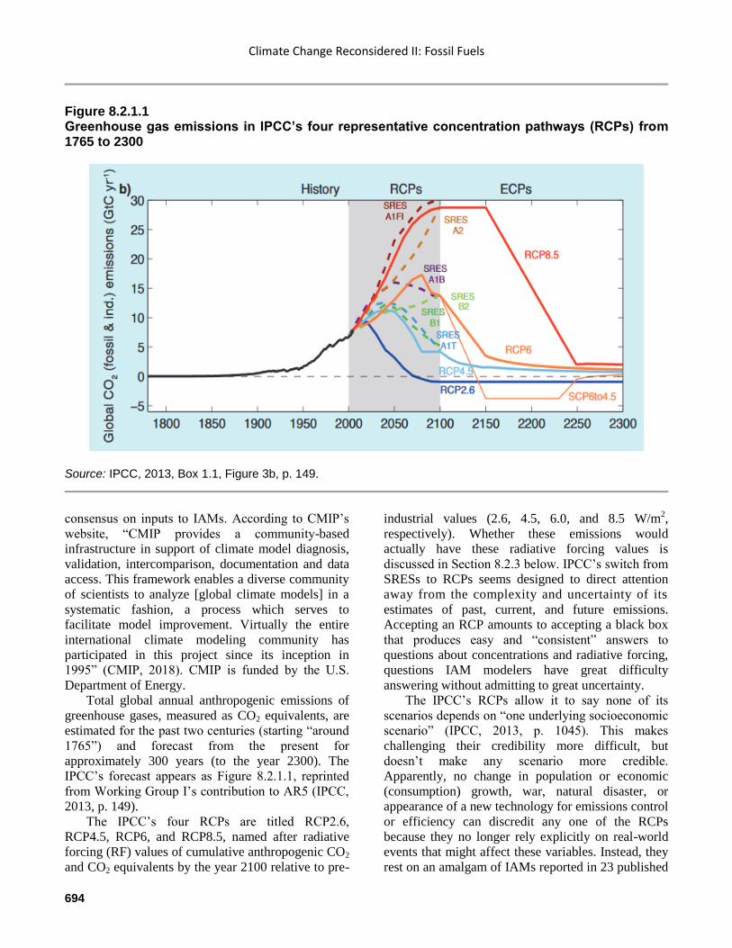
Climate Change Reconsidered II: Fossil Fuels

694

Figure 8.2.1.1 Greenhouse gas emissions in IPCC’s four representative concentration pathways (RCPs) from 1765 to 2300

Source: IPCC, 2013, Box 1.1, Figure 3b, p. 149.

consensus on inputs to IAMs. According to CMIP’s

website, “CMIP provides a community-based

infrastructure in support of climate model diagnosis,

validation, intercomparison, documentation and data

access. This framework enables a diverse community

of scientists to analyze [global climate models] in a

systematic fashion, a process which serves to

facilitate model improvement. Virtually the entire

international climate modeling community has

participated in this project since its inception in

1995” (CMIP, 2018). CMIP is funded by the U.S.

Department of Energy.

Total global annual anthropogenic emissions of

greenhouse gases, measured as CO2 equivalents, are

estimated for the past two centuries (starting “around

1765”) and forecast from the present for

approximately 300 years (to the year 2300). The

IPCC’s forecast appears as Figure 8.2.1.1, reprinted

from Working Group I’s contribution to AR5 (IPCC,

2013, p. 149).

The IPCC’s four RCPs are titled RCP2.6,

RCP4.5, RCP6, and RCP8.5, named after radiative

forcing (RF) values of cumulative anthropogenic CO2

and CO2 equivalents by the year 2100 relative to pre-

industrial values (2.6, 4.5, 6.0, and 8.5 W/m2,

respectively). Whether these emissions would

actually have these radiative forcing values is

discussed in Section 8.2.3 below. IPCC’s switch from

SRESs to RCPs seems designed to direct attention

away from the complexity and uncertainty of its

estimates of past, current, and future emissions.

Accepting an RCP amounts to accepting a black box

that produces easy and “consistent” answers to

questions about concentrations and radiative forcing,

questions IAM modelers have great difficulty

answering without admitting to great uncertainty.

The IPCC’s RCPs allow it to say none of its

scenarios depends on “one underlying socioeconomic

scenario” (IPCC, 2013, p. 1045). This makes

challenging their credibility more difficult, but

doesn’t make any scenario more credible.

Apparently, no change in population or economic

(consumption) growth, war, natural disaster, or

appearance of a new technology for emissions control

or efficiency can discredit any one of the RCPs

because they no longer rely explicitly on real-world

events that might affect these variables. Instead, they

rest on an amalgam of IAMs reported in 23 published

Cost-Benefit Analysis

695

reports (see sources cited for Table 12.1 on pp. 1048–

49). This resembles the IPCC’s decision to rely on

the DICE, FUND, and PAGE models for its cost-

benefit analysis. But what is convenient for modelers

is not necessarily good science. Once again,

averaging the outputs of models that share common

flaws does not produce results more accurate than

any one model can produce.

Forecasting future emissions is no easy task

given the crude and often simplified

parameterizations utilized by IAMs to mimic the

global economy (Lemoine and Rudik, 2017). The key

is to accurately portray the quantity of current and

annual future emissions by properly estimating future

population and economic growth and changes in

technology and productivity, and predicting

seemingly unpredictable events such as changes in

government policies, wars, scientific and medical

breakthroughs, and more. Few self-described

“futurists” can accurately predict such things a year

or two in advance. None can predict them across

decades or even centuries, as the IPCC attempts to

do.

Even measuring current emissions is an

extremely complex and difficult exercise. Because

natural sources (oceans and vegetation) produce

massive amounts of CO2 relative to human emissions,

their background presence makes the measurement of

anthropogenic emissions on the ground impossible.

As reported in Chapter 5, Section 5.1.2, human CO2

emissions account for only about 3.5% (7.8 Gt

divided by 220 Gt) of the carbon entering the

atmosphere each year and so, with about 0.5% (1.1

Gt divided by 220 Gt) from net land use change,

natural sources account for the remaining 96.0%. The

residual of the human contribution the IPCC believes

remains in the atmosphere after natural processes

move the rest to other reservoirs is as little as 1.17 Gt

per year (15% of 7.8 Gt), just 0.53% of the carbon

entering the atmosphere each year (IPCC, 2013, p.

471, Figure 6.1). This is less than two-tenths of 1%

(0.195%) of the total amount of carbon thought to be

in the atmosphere.

Of course, the IPCC does not actually measure

CO2 emissions, since there are millions of sources

(billions if humans are counted). Virtually all

emission estimates coming from CMIP and therefore

the IPCC are not observational data, but stylized facts

standing in for unknown quantities that can only be

estimated by models and formulas homogenizing

disparate and often poorly maintained databases. As

the IPCC says, “the final RCP data sets comprise

land use data, harmonized GHG emissions and

concentrations, gridded reactive gas and aerosol

emissions, as well as ozone and aerosol abundance

fields” (p. 1046).

Not all countries are able to keep accurate

records of economic activity, much less emissions of

a dozen gases. “Informal economies” constitute a

large part of the economies of many developing and

even industrial countries, and little is known about

their use of natural resources or emissions. It is

thought that 50% of the world’s workforce works in

informal markets and are likely to escape government

regulations and reporting requirements (Jutting and

de Laiglesia, 2009). If their use of energy and

emissions are comparable to use in the formal

economy, then an economy as large as that of China

and Japan combined is largely invisible to

government data collectors. This source of

uncertainty is never reported by IAM modelers.

Some countries, including major emitters such as

China and Russia, routinely manipulate data

regarding economic growth and investment to hide

economic woes from their citizens or exaggerate their

success to other world leaders. Martinez (2018)

observes that totalitarian regimes have “a stronger

incentive to exaggerate economic performance (years

of low growth, before elections, after becoming

ineligible for foreign aid)” which might be observed

in their reporting of “GDP sub-components that rely

on government information and have low third-party

verification.” To measure this deception, he

compared satellite images of changes over time in

electric lights in free and authoritarian countries to

their reported economic growth rates during the same

period. He found that “yearly GDP growth rates are

inflated by a factor of between 1.15 and 1.3 in the

most authoritarian regimes” (Martinez, 2018; see also

Ingraham, 2018). According to Freedom House, an

organization that monitors democracy and

authoritarianism around the world, countries

designated as “free” in 2013 represented only 40% of

the global population (Freedom House, 2014).

With respect to economic growth, IAMs typically

assume compound annual global economic growth

rates for the period 1995 to 2100 that range between

1.48% and 2.45%, with an average baseline rate of

growth of 2.17%. Spreadsheets with the various

parameters for the created scenarios can be found on

a website maintained by the Energy Modeling Forum

at Stanford University (Energy Modeling Forum,

2018). These rates of growth are not particularly

high, especially when compared to global growth

rates over the past 50 years. The International Energy

Agency (IEA) assumes that world GDP, in

Climate Change Reconsidered II: Fossil Fuels

696

purchasing power parity (PPP), will grow by an

average of 3.4% annually over the period 2010–2030

(IEA, 2017). Similarly, the U.S. Energy Information

Agency (EIA) forecasts that from 2015 to 2040, real

world GDP growth averages 3.0% in its Reference

case (EIA, 2017). If a warmer world is also a more

prosperous world, as countless historians have

documented was the case in the past (see the review

in Chapter 7), then even these projected rates will be

too low and along with them, forecasts of future

greenhouse gas emissions.

More rapid-than-expected technological change

would have the opposite effect of faster-than-

expected economic growth. Thanks to the spread of

electrification, technology-induced energy efficiency,

and the emergence of natural gas as a vigorous

competitor to coal for electricity production in the

United States (and likely in other countries in the

future), the correlation between economic growth

(consumption) and greenhouse gas emissions has

weakened since the end of the twentieth century

(Handrich et al., 2015). Emissions in industrialized

countries generally, and especially in the United

States, have slowed or even fallen despite population

and consumption growth, evidence of the

“dematerialization” reported by Ausubel and

Waggoner (2008), Goklany (2009), Smil (2013), and

others cited in Chapter 5.

In conclusion, most IAMs rely on emission

scenarios that are little more than guesses and

speculative “storylines.” Even current greenhouse gas

emissions cannot be measured accurately, and

technology is likely to change future emissions in

ways that cannot be predicted.

References

Ausubel, J.H. and Waggoner, P. 2008. Dematerialization:

variety, caution, and persistence. Proceedings of the

National Academy of Sciences USA 105 (35): 12,774–

12,779.

CMIP. 2018. About CMIP (website). Accessed June 27,

2018.

EIA. 2017. U.S. Energy Information Administration. 2017

International Energy Outlook.

Energy Modeling Forum. 2018. About (website). Stanford,

CA: Stanford University. Accessed June 29, 2018.

Freedom House. 2014. Freedom in the world: 2014. Fact

Sheet (website). Accessed July 4, 2018.

Goklany, I.M. 2009. Have increases in population,

affluence and technology worsened human and

environmental well-being? The Electronic Journal of

Sustainable Development 1 (3): 3–28.

Handrich, L., Kemfert, C., Mattes, A., Pavel, F., and

Traber, T. 2015. Turning Point: Decoupling Greenhouse

Gas Emissions from Economic Growth. A study by DIW

Econ. Berlin, Germany: Heinrich Böll Stiftung.

IEA. 2017. International Energy Agency. World Energy

Outlook.

Ingraham, C. 2018. Satellite data strongly suggests that

China, Russia and other authoritarian countries are fudging

their GDP reports. Washington Post. May 15.

IPCC. 2000. Intergovernmental Panel on Climate Change.

IPCC Special Report: Emissions Scenarios. A Special

Report of IPCC Working Group III. Cambridge, UK:

Cambridge University Press.

IPCC. 2013. Intergovernmental Panel on Climate Change.

Climate Change 2013: The Physical Science Basis.

Contribution of Working Group I to the Fifth Assessment

Report of the Intergovernmental Panel on Climate Change.

Cambridge, UK: Cambridge University Press.

Jutting, J. and de Laiglesia, J.R. (Eds.) 2009. Is Informal

Normal? Towards More and Better Jobs in Developing

Countries. Paris, France: Organization for Economic

Cooperation and Development.

Lemoine, D.M. and Rudik, I. 2017. Steering the climate

system: using inertia to lower the cost of policy. American

Economic Review 107 (10): 2947–57.

Martinez, L.R. 2018. How much should we trust the

dictator’s GDP estimates? University of Chicago Irving B.

Harris Graduate School of Public Policy Studies, May 1.

Available at SSRN: https://ssrn.com/abstract=3093296.

Smil, V. 2013. Making the Modern World: Materials and

Dematerialization. New York, NY: Wiley.

8.2.2 Carbon Cycle

IAMs falsely assume the carbon cycle is

sufficiently understood and measured with

sufficient accuracy as to make possible

precise predictions of future levels of carbon

dioxide (CO2) in the atmosphere.

As illustrated in Figure 8.1.2.1.1, the second step in

an IAM is to compute the trajectory of global

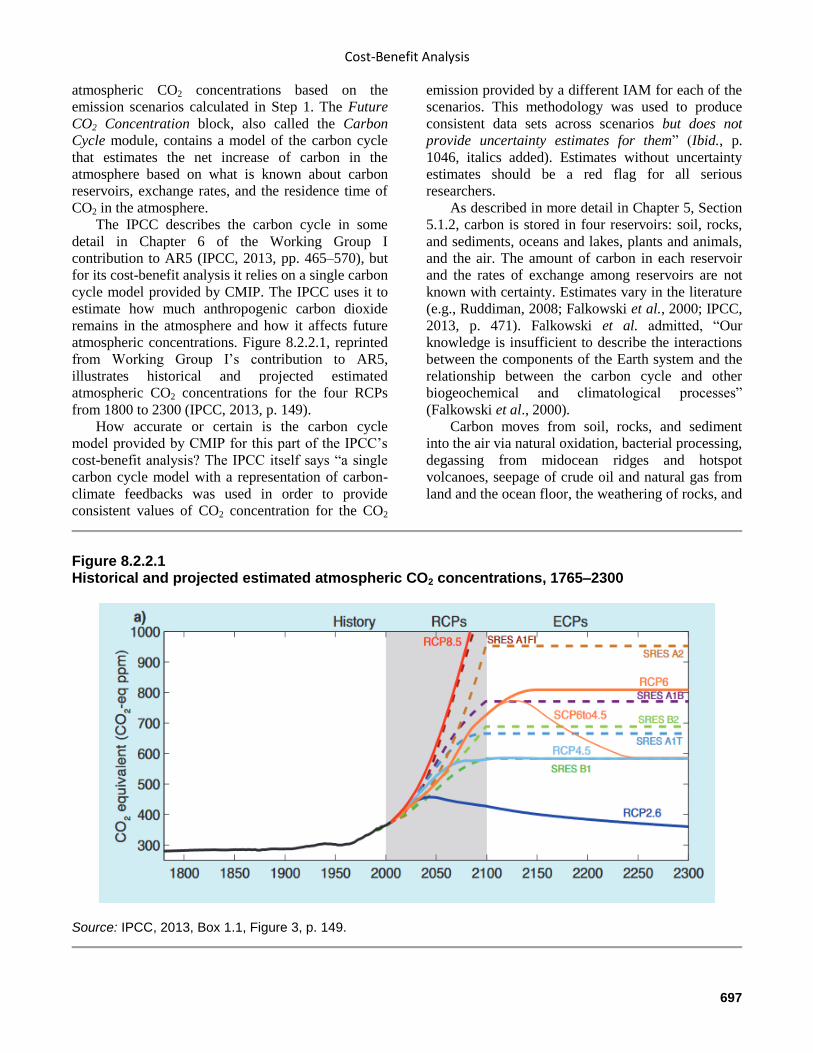
Cost-Benefit Analysis

697

atmospheric CO2 concentrations based on the

emission scenarios calculated in Step 1. The Future

CO2 Concentration block, also called the Carbon

Cycle module, contains a model of the carbon cycle

that estimates the net increase of carbon in the

atmosphere based on what is known about carbon

reservoirs, exchange rates, and the residence time of

CO2 in the atmosphere.

The IPCC describes the carbon cycle in some

detail in Chapter 6 of the Working Group I

contribution to AR5 (IPCC, 2013, pp. 465–570), but

for its cost-benefit analysis it relies on a single carbon

cycle model provided by CMIP. The IPCC uses it to

estimate how much anthropogenic carbon dioxide

remains in the atmosphere and how it affects future

atmospheric concentrations. Figure 8.2.2.1, reprinted

from Working Group I’s contribution to AR5,

illustrates historical and projected estimated

atmospheric CO2 concentrations for the four RCPs

from 1800 to 2300 (IPCC, 2013, p. 149).

How accurate or certain is the carbon cycle

model provided by CMIP for this part of the IPCC’s

cost-benefit analysis? The IPCC itself says “a single

carbon cycle model with a representation of carbon-

climate feedbacks was used in order to provide

consistent values of CO2 concentration for the CO2

emission provided by a different IAM for each of the

scenarios. This methodology was used to produce

consistent data sets across scenarios but does not

provide uncertainty estimates for them” (Ibid., p.

1046, italics added). Estimates without uncertainty

estimates should be a red flag for all serious

researchers.

As described in more detail in Chapter 5, Section

5.1.2, carbon is stored in four reservoirs: soil, rocks,

and sediments, oceans and lakes, plants and animals,

and the air. The amount of carbon in each reservoir

and the rates of exchange among reservoirs are not

known with certainty. Estimates vary in the literature

(e.g., Ruddiman, 2008; Falkowski et al., 2000; IPCC,

2013, p. 471). Falkowski et al. admitted, “Our

knowledge is insufficient to describe the interactions

between the components of the Earth system and the

relationship between the carbon cycle and other

biogeochemical and climatological processes”

(Falkowski et al., 2000).

Carbon moves from soil, rocks, and sediment

into the air via natural oxidation, bacterial processing,

degassing from midocean ridges and hotspot

volcanoes, seepage of crude oil and natural gas from

land and the ocean floor, the weathering of rocks, and

Figure 8.2.2.1 Historical and projected estimated atmospheric CO2 concentrations, 1765–2300

Source: IPCC, 2013, Box 1.1, Figure 3, p. 149.

Climate Change Reconsidered II: Fossil Fuels

698

burning of fossil fuels. Just how much carbon is

released naturally from the lithosphere in any given

year is uncertain. According to Burton et al. (2013, p.

323), “the role of CO2 degassing from the Earth is

clearly fundamental to the stability of the climate,

and therefore to life on Earth. Notwithstanding this

importance, the flux of CO2 from the Earth is poorly

constrained. The uncertainty in our knowledge of this

critical input into the geological carbon cycle led

Berner and Lagasa (1989) to state that it is the most

vexing problem facing us in understanding that

cycle.”

According to Wylie (2013), estimates of volcanic

degassing rose from around 100 million metric tons

of CO2 per year in 1992 to 600 million metric tons in

2013, a six-fold increase in two decades. According

to Aminzadeh et al. (2013, p. 4), “What is the volume

of hydrocarbon seepage worldwide? The Coal Oil

Point seeps are a large source of air pollution in Santa

Barbara County, California. Those seeps are similar

in many ways to the seeps discussed in this volume.

When multiplied by any reasonable assumption of

seep numbers worldwide, it is easy to imagine that

natural seepage of oil in the range of thousands of

barrels per day and gas leakage of hundreds of

millions of cubic feet per day is not unreasonable.”

In 2003, a U.S. National Research Council report

titled Oil in the Sea III acknowledged “the inputs

from land-based sources are poorly understood, and

therefore estimates of these inputs have a high degree

of uncertainty,” and “estimating the amount of

natural seepage of crude oil into the marine

environment involves broad extrapolations from

minimal data.” It nevertheless estimated the annual

global oil seepage rate to be between 200,000 and

2,000,000 tons (60 and 600 million gallons) (NRC,

2003). Since the NRC report was produced, extensive

use by the oil industry of 3D seismic data, manned

submersibles, and remotely operated vehicles has

revealed more seeps than previously assumed to

exist, suggesting natural seepage of hydrocarbons

from the ocean floor may be understated by the IPCC

and other research bodies (Roberts and Feng, 2013, p.

56).

Oceans are the second largest reservoir of carbon,

containing about 65 times as much as the air. The

IPCC and other political and scientific bodies assume

roughly 50% to 70% (note the range) of the CO2

produced by human combustion of fossil fuels is

absorbed and sequestered by the oceans, most of the

remainder is taken up by plants and animals

(terrestrial as well as aquatic), and what’s left

remains in the air, contributing to the slow increase in

atmospheric concentrations of CO2 during the modern

era.

Earth’s atmosphere (air) is the fourth and

smallest reservoir, estimated to hold approximately

870 gigatons of carbon (GtC). (Note this estimate is

generated by mathematical formulas and is not

observational data.) As mentioned in the previous

section, the total human contribution, including net

land use change (primarily agriculture and forestry),

is only about 4.3% of total annual releases of carbon

into the atmosphere (IPCC, 2013, p. 471, Figure 6.1).

The residual of the human contribution that the IPCC

believes remains in the atmosphere after natural

processes move the rest to other reservoirs is just

0.53% of the carbon entering the air each year. It is

less than two-tenths of 1% (0.195%) of the total

amount of carbon thought to be in the atmosphere,

per Ruddiman (2008). Given uncertainties in the

sizes of the reservoirs and the exchange rates among

them, it is proper to ask if this residual is measurable,

and if not, if it exists at all.

The IPCC apparently assumes atmospheric CO2

concentrations would be stable, decade after decade

and century after century, but for anthropogenic

emissions. Yet research suggests 500 million years

ago the atmosphere’s CO2 concentration was

approximately 20 times higher than it is today, at

around 7,500 ppm. Two hundred million years later it

declined to close to the air’s current CO2

concentration of just over 400 ppm, after which it

rose to four times that amount at 220 million years

before present (Berner, 1990, 1992, 1993, 1997;

Kasting, 1993).

During the middle Eocene, some 43 million years

ago, the atmospheric CO2 concentration is estimated

to have dropped to a mean value of approximately

385 ppm (Pearson and Palmer, 1999), and between

25 to nine million years ago, it is believed to have

varied between 180ppm and 290 ppm (Pagani et al.,

1999). This latter concentration range is essentially

the same in which the air’s CO2 concentration

oscillated during the 100,000-year glacial cycles of

the past 420,000 years (Fischer et al., 1999; Petit et

al., 1999). While the natural processes that have

driven these changes in CO2 are not likely to operate

over the shorter time scales of an IAM, they

nonetheless demonstrate the natural world can and

does influence the atmosphere’s CO2 content.

But there is also evidence nature’s carbon cycle

can impact atmospheric CO2 at the shorter time

periods that matter to IAMs. Joos and Bruno (1998)

used ice core data and direct observations of

atmospheric CO2 and 13

C to reconstruct the histories

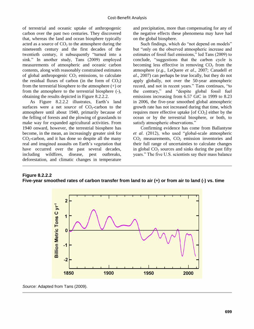
Cost-Benefit Analysis

699

of terrestrial and oceanic uptake of anthropogenic

carbon over the past two centuries. They discovered

that, whereas the land and ocean biosphere typically

acted as a source of CO2 to the atmosphere during the

nineteenth century and the first decades of the

twentieth century, it subsequently “turned into a

sink.” In another study, Tans (2009) employed

measurements of atmospheric and oceanic carbon

contents, along with reasonably constrained estimates

of global anthropogenic CO2 emissions, to calculate

the residual fluxes of carbon (in the form of CO2)

from the terrestrial biosphere to the atmosphere (+) or

from the atmosphere to the terrestrial biosphere (-),

obtaining the results depicted in Figure 8.2.2.2.

As Figure 8.2.2.2 illustrates, Earth’s land

surfaces were a net source of CO2-carbon to the

atmosphere until about 1940, primarily because of

the felling of forests and the plowing of grasslands to

make way for expanded agricultural activities. From

1940 onward, however, the terrestrial biosphere has

become, in the mean, an increasingly greater sink for

CO2-carbon, and it has done so despite all the many

real and imagined assaults on Earth’s vegetation that

have occurred over the past several decades,

including wildfires, disease, pest outbreaks,

deforestation, and climatic changes in temperature

and precipitation, more than compensating for any of

the negative effects these phenomena may have had

on the global biosphere.

Such findings, which do “not depend on models”

but “only on the observed atmospheric increase and

estimates of fossil fuel emissions,” led Tans (2009) to

conclude, “suggestions that the carbon cycle is

becoming less effective in removing CO2 from the

atmosphere (e.g., LeQuere et al., 2007; Canadell et

al., 2007) can perhaps be true locally, but they do not

apply globally, not over the 50-year atmospheric

record, and not in recent years.” Tans continues, “to

the contrary,” and “despite global fossil fuel

emissions increasing from 6.57 GtC in 1999 to 8.23

in 2006, the five-year smoothed global atmospheric

growth rate has not increased during that time, which

requires more effective uptake [of CO2] either by the

ocean or by the terrestrial biosphere, or both, to

satisfy atmospheric observations.”

Confirming evidence has come from Ballantyne

et al. (2012), who used “global-scale atmospheric

CO2 measurements, CO2 emission inventories and

their full range of uncertainties to calculate changes

in global CO2 sources and sinks during the past fifty

years.” The five U.S. scientists say their mass balance

Figure 8.2.2.2 Five-year smoothed rates of carbon transfer from land to air (+) or from air to land (-) vs. time

Source: Adapted from Tans (2009).

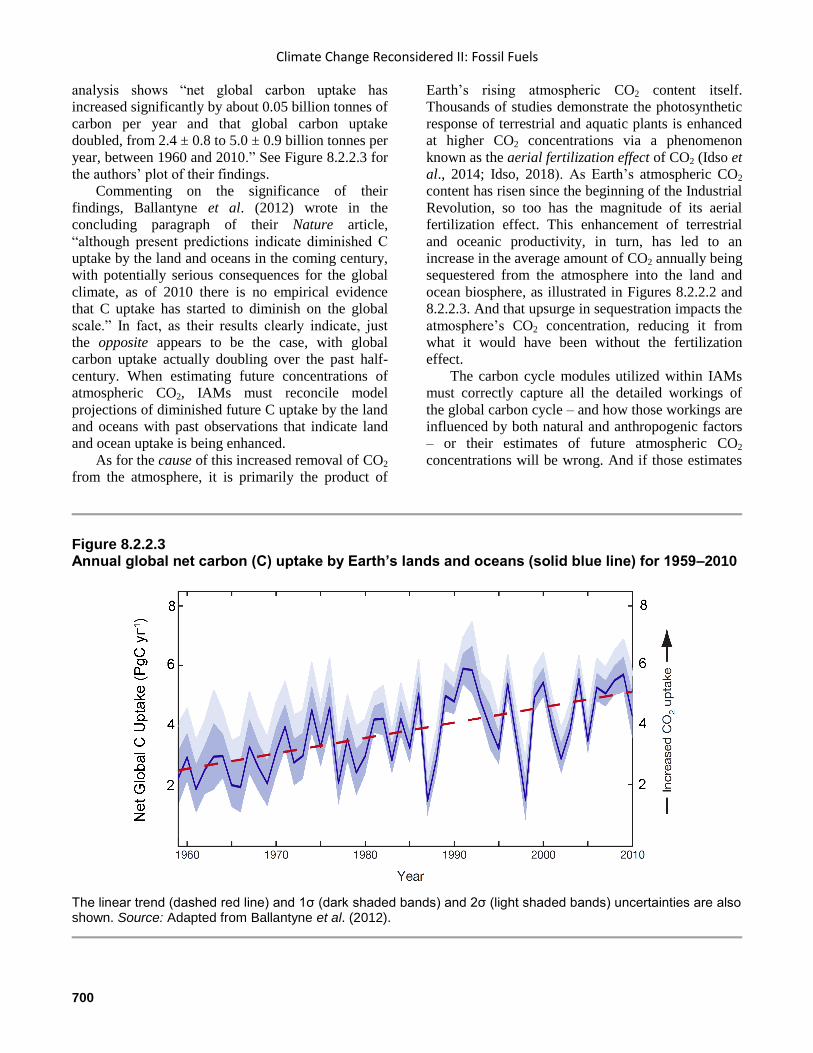
Climate Change Reconsidered II: Fossil Fuels

700

analysis shows “net global carbon uptake has

increased significantly by about 0.05 billion tonnes of

carbon per year and that global carbon uptake

doubled, from 2.4 ± 0.8 to 5.0 ± 0.9 billion tonnes per

year, between 1960 and 2010.” See Figure 8.2.2.3 for

the authors’ plot of their findings.

Commenting on the significance of their

findings, Ballantyne et al. (2012) wrote in the

concluding paragraph of their Nature article,

“although present predictions indicate diminished C

uptake by the land and oceans in the coming century,

with potentially serious consequences for the global

climate, as of 2010 there is no empirical evidence

that C uptake has started to diminish on the global

scale.” In fact, as their results clearly indicate, just

the opposite appears to be the case, with global

carbon uptake actually doubling over the past half-

century. When estimating future concentrations of

atmospheric CO2, IAMs must reconcile model

projections of diminished future C uptake by the land

and oceans with past observations that indicate land

and ocean uptake is being enhanced.

As for the cause of this increased removal of CO2

from the atmosphere, it is primarily the product of

Earth’s rising atmospheric CO2 content itself.

Thousands of studies demonstrate the photosynthetic

response of terrestrial and aquatic plants is enhanced

at higher CO2 concentrations via a phenomenon

known as the aerial fertilization effect of CO2 (Idso et

al., 2014; Idso, 2018). As Earth’s atmospheric CO2

content has risen since the beginning of the Industrial

Revolution, so too has the magnitude of its aerial

fertilization effect. This enhancement of terrestrial

and oceanic productivity, in turn, has led to an

increase in the average amount of CO2 annually being

sequestered from the atmosphere into the land and

ocean biosphere, as illustrated in Figures 8.2.2.2 and

8.2.2.3. And that upsurge in sequestration impacts the

atmosphere’s CO2 concentration, reducing it from

what it would have been without the fertilization

effect.

The carbon cycle modules utilized within IAMs

must correctly capture all the detailed workings of

the global carbon cycle – and how those workings are

influenced by both natural and anthropogenic factors

– or their estimates of future atmospheric CO2

concentrations will be wrong. And if those estimates

Figure 8.2.2.3 Annual global net carbon (C) uptake by Earth’s lands and oceans (solid blue line) for 1959–2010

The linear trend (dashed red line) and 1σ (dark shaded bands) and 2σ (light shaded bands) uncertainties are also shown. Source: Adapted from Ballantyne et al. (2012).

Cost-Benefit Analysis

701

are inaccurate, so will be the projected impacts of

future climate that depend on them. No current IAM

incorporates this moderating influence of the aerial

fertilization effect on future CO2 concentrations.

In conclusion, IAMs falsely assume the carbon

cycle is sufficiently understood and measured with

sufficient accuracy as to make possible precise

predictions of future levels of CO2 in the atmosphere.

References

Aminzadeh, F., Berge, T.B., and Connolly, D.L. (Eds.)

2013. Hydrocarbon Seepage: From Source to Surface.

Geophysical Developments Series No. 16. Tulsa, OK:

Society of Exploration Geophysicists and American

Association of Petroleum Geologists.

Ballantyne, A.P., Alden, C.B., Miller, J.B., Tans, P.P., and

White, J.W. 2012. Increase in observed net carbon dioxide

uptake by land and oceans during the past 50 years. Nature

488: 70–2.

Berner, R.A. 1990. Atmospheric carbon dioxide levels

over Phanerozoic time. Science 249: 1382–6.

Berner, R.A. 1992. Paleo-CO2 and climate. Nature 358:

114.

Berner, R.A. 1993. Paleozoic atmospheric CO2:

importance of solar radiation and plant evolution. Science

261: 68–70.

Berner, R.A. 1997. The rise of plants and their effect on

weathering and atmospheric CO2. Science 276: 544–6.

Berner R.A. and Lasaga, A.C. 1989. Modeling the

geochemical carbon cycle. Scientific American 260:74–81.

Burton, M.R., Sawyer, G.M., and Granieri, D. 2013. Deep

carbon emissions from volcanoes. Reviews in Mineralogy

and Geochemistry 75 (1): 323–54.

Canadell, J.G., et al. 2007. Contributions to accelerating

atmospheric CO2 growth from economic activity, carbon

intensity, and efficiency of natural sinks. Proceedings of

the National Academy of Sciences USA 104: 18,866–70.

Falkowski, P., et al. 2000. The global carbon cycle: a test

of our knowledge of Earth as a system. Science 290

(5490): 291–96.

Fischer, H., Wahlen, M., Smith, J., Mastroianni, D., and

Deck, B. 1999. Ice core records of atmospheric CO2

around the last three glacial terminations. Science 283:

1712–4.

Idso, C.D. 2018. CO2 Science Plant Growth Study

Database (website). Accessed June 29.

Idso, C.D., Idso, S.B., Carter, R.M., and S.F. Singer. 2014.

(Eds.) Nongovernmental International Panel on Climate

Change. Climate Change Reconsidered II: Biological

Impacts. Chicago, IL: The Heartland Institute.

IPCC. 2013. Intergovernmental Panel on Climate Change.

Climate Change 2013: The Physical Science Basis.

Contribution of Working Group I to the Fifth Assessment

Report of the Intergovernmental Panel on Climate Change.

Cambridge, UK: Cambridge University Press.

Joos, F. and Bruno, M. 1998. Long-term variability of the

terrestrial and oceanic carbon sinks and the budgets of the

carbon isotopes 13

C and 14

C. Global Biogeochemical

Cycles 12: 277–95.

Kasting, J.F. 1993. Earth’s early atmosphere. Science 259:

920–6.

Le Quere, C., et al. 2007. Saturation of the Southern Ocean

CO2 sink due to recent climate change. Science 316: 1735–

8.

NRC. 2003. U.S. National Research Council Committee

on Oil in the Sea. Oil in the Sea III: Inputs, Fates, and

Effects. Washington, DC: National Academies Press.

Pagani, M., Arthur, M.A., and Freeman, K.H. 1999.

Miocene evolution of atmospheric carbon dioxide.

Paleoceanography 14: 273–92.

Pearson, P.N. and Palmer, M.R. 1999. Middle Eocene

seawater pH and atmospheric carbon dioxide

concentrations. Science 284: 1824–6.

Petit, J.R., et al. 1999. Climate and atmospheric history of

the past 420,000 years from the Vostok ice core,

Antarctica. Nature 399: 429–36.

Roberts, H.H. and Feng, D. 2013. Carbonate precipitation

at Gulf of Mexico hydrocarbon seeps: an overview. In:

Aminzadeh, F., Berge, T.B., and Connolly, D.L. (Eds.).

Hydrocarbon Seepage: From Source to Surface.

Geophysical Developments Series No. 16. Tulsa, OK:

Society of Exploration Geophysicists and American

Association of Petroleum Geologists, pp. 43–61.

Ruddiman, W.F. 2008. Earth’s Climate: Past and Future.

Second edition. New York, NY: W.H. Freeman and

Company.

Tans, P. 2009. An accounting of the observed increase in

oceanic and atmospheric CO2 and an outlook for the

future. Oceanography 22: 26–35.

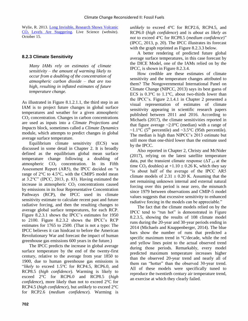
Climate Change Reconsidered II: Fossil Fuels

702

Wylie, R. 2013. Long Invisible, Research Shows Volcanic

CO2 Levels Are Staggering. Live Science (website).

October 15.

8.2.3 Climate Sensitivity

Many IAMs rely on estimates of climate

sensitivity – the amount of warming likely to

occur from a doubling of the concentration of

atmospheric carbon dioxide – that are too

high, resulting in inflated estimates of future

temperature change.

As illustrated in Figure 8.1.2.1.1, the third step in an

IAM is to project future changes in global surface

temperatures and weather for a given atmospheric

CO2 concentration. Changes in carbon concentrations

are used as inputs into a Climate Projections and

Impacts block, sometimes called a Climate Dynamics

module, which attempts to predict changes in global

average surface temperature.

Equilibrium climate sensitivity (ECS) was

discussed in some detail in Chapter 2. It is broadly

defined as the equilibrium global mean surface

temperature change following a doubling of

atmospheric CO2 concentration. In its Fifth

Assessment Report (AR5), the IPCC decided on “a

range of 2°C to 4.5°C, with the CMIP5 model mean

at 3.2°C” (IPCC, 2013, p. 83). Having estimated the

increase in atmospheric CO2 concentrations caused

by emissions in its four Representative Concentration

Pathways (RCP), the IPCC used its climate

sensitivity estimate to calculate recent past and future

radiative forcing, and then the resulting changes to

average global surface temperatures, for each RCP.

Figure 8.2.3.1 shows the IPCC’s estimates for 1950

to 2100. Figure 8.2.3.2 shows the IPCC’s RCP

estimates for 1765 to 2500. (That is not a typo: The

IPCC believes it can hindcast to before the American

Revolutionary War and forecast the impact of human

greenhouse gas emissions 600 years in the future.)

The IPCC predicts the increase in global average

surface temperature by the end of the twenty-first

century, relative to the average from year 1850 to

1900, due to human greenhouse gas emissions is

“likely to exceed 1.5°C for RCP4.5, RCP6.0, and

RCP8.5 (high confidence). Warming is likely to

exceed 2°C for RCP6.0 and RCP8.5 (high

confidence), more likely than not to exceed 2°C for

RCP4.5 (high confidence), but unlikely to exceed 2°C

for RCP2.6 (medium confidence). Warming is

unlikely to exceed 4°C for RCP2.6, RCP4.5, and

RCP6.0 (high confidence) and is about as likely as

not to exceed 4°C for RCP8.5 (medium confidence)”

(IPCC, 2013, p. 20). The IPCC illustrates its forecast

with the graph reprinted as Figure 8.2.3.3 below.

A better rendering of predicted future global

average surface temperatures, in this case forecast by

the DICE Model, one of the IAMs relied on by the

IPCC, is shown in Figure 8.2.3.4.

How credible are these estimates of climate

sensitivity and the temperature changes attributed to

them? The Nongovernmental International Panel on

Climate Change (NIPCC, 2013) says its best guess of

ECS is 0.3°C to 1.1°C, about two-thirds lower than

the IPCC’s. Figure 2.1.4.1 in Chapter 2 presented a

visual representation of estimates of climate

sensitivity appearing in scientific research papers

published between 2011 and 2016. According to

Michaels (2017), the climate sensitivities reported in

that figure average ~2.0°C (median) with a range of

~1.1°C (5th percentile) and ~3.5°C (95th percentile).

The median is high than NIPCC’s 2013 estimate but

still more than one-third lower than the estimate used

by the IPCC.

Also reported in Chapter 2, Christy and McNider

(2017), relying on the latest satellite temperature

data, put the transient climate response (ΔT LT at the

time CO2 doubles) at +1.10 ± 0.26 K, which they say

“is about half of the average of the IPCC AR5

climate models of 2.31 ± 0.20 K. Assuming that the

net remaining unknown internal and external natural

forcing over this period is near zero, the mismatch

since 1979 between observations and CMIP-5 model

values suggests that excessive sensitivity to enhanced

radiative forcing in the models can be appreciable.”

The fact that the climate models relied on by the

IPCC tend to “run hot” is demonstrated in Figure

8.2.3.5, showing the results of 108 climate model

runs during the 20-year and 30-year periods ending in

2014 (Michaels and Knappenberger, 2014). The blue

bars show the number of runs that predicted a

specific maximum trend in °C/decade, while the red

and yellow lines point to the actual observed trend

during those periods. Remarkably, every model

predicted maximum temperature increases higher

than the observed 20-year trend and nearly all of

them ran “hotter” than the observed 30-year trend.

All of these models were specifically tuned to

reproduce the twentieth century air temperature trend,

an exercise at which they clearly failed.

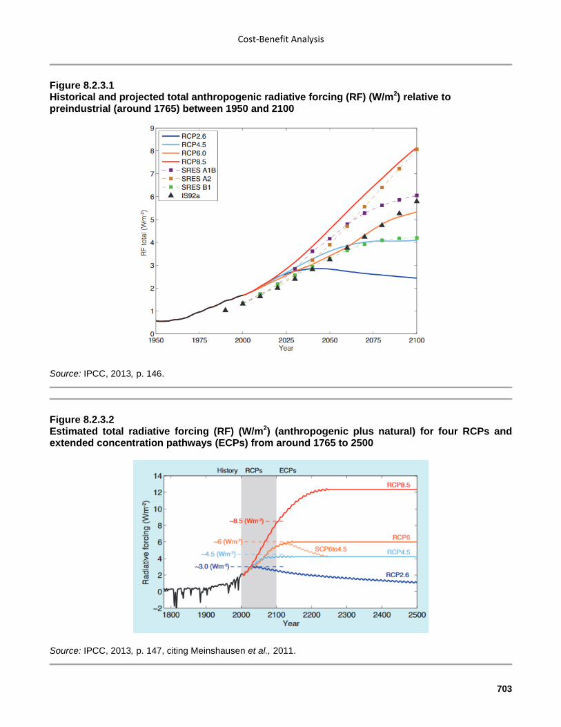
Cost-Benefit Analysis

703

Figure 8.2.3.1 Historical and projected total anthropogenic radiative forcing (RF) (W/m2) relative to preindustrial (around 1765) between 1950 and 2100

Source: IPCC, 2013, p. 146.

Figure 8.2.3.2 Estimated total radiative forcing (RF) (W/m2) (anthropogenic plus natural) for four RCPs and extended concentration pathways (ECPs) from around 1765 to 2500

Source: IPCC, 2013, p. 147, citing Meinshausen et al., 2011.

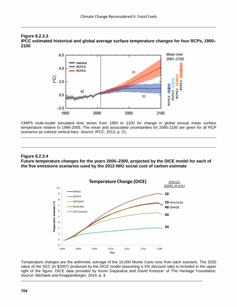
Climate Change Reconsidered II: Fossil Fuels

704

Figure 8.2.3.3 IPCC estimated historical and global average surface temperature changes for four RCPs, 1950–2100

CMIP5 multi-model simulated time series from 1950 to 2100 for change in global annual mean surface temperature relative to 1986-2005. The mean and associated uncertainties for 2085-2100 are given for all RCP scenarios as colored vertical bars. Source: IPCC, 2013, p. 21.

Figure 8.2.3.4 Future temperature changes for the years 2000–2300, projected by the DICE model for each of the five emissions scenarios used by the 2013 IWG social cost of carbon estimate

Temperature changes are the arithmetic average of the 10,000 Monte Carlo runs from each scenario. The 2020 value of the SCC (in $2007) produced by the DICE model (assuming a 3% discount rate) is included in the upper right of the figure. DICE data provided by Kevin Dayaratna and David Kreutzer of The Heritage Foundation. Source: Michaels and Knappenberger, 2014, p. 4.

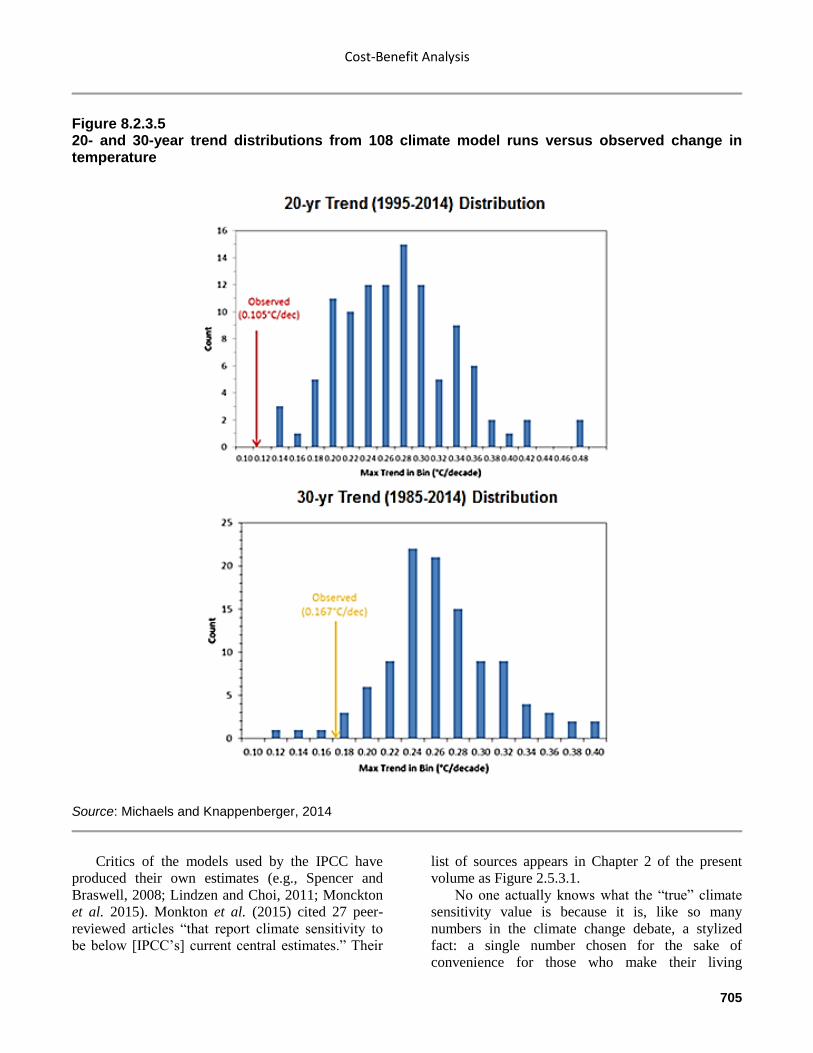
Cost-Benefit Analysis

705

Figure 8.2.3.5 20- and 30-year trend distributions from 108 climate model runs versus observed change in temperature

Source: Michaels and Knappenberger, 2014

Critics of the models used by the IPCC have

produced their own estimates (e.g., Spencer and

Braswell, 2008; Lindzen and Choi, 2011; Monckton

et al. 2015). Monkton et al. (2015) cited 27 peer-

reviewed articles “that report climate sensitivity to

be below [IPCC’s] current central estimates.” Their

list of sources appears in Chapter 2 of the present

volume as Figure 2.5.3.1.

No one actually knows what the “true” climate

sensitivity value is because it is, like so many

numbers in the climate change debate, a stylized

fact: a single number chosen for the sake of

convenience for those who make their living

Climate Change Reconsidered II: Fossil Fuels

706

modeling climate change. The number is inherently

uncertain for much the same reason it is impossible

to know how much CO2 is emitted into the air every

year or how much of it stays there, which is the

enormous size of natural processes relative to the

“human signal” caused by our CO2 emissions

(Frank, 2015). See Chapter 2, Section 2.2.3 for a

discussion of climate sensitivity, and more generally

NIPCC (2013) for hundreds of source citations on

this complex matter.

The IPCC’s estimate of climate sensitivity is

very likely to be too high, which invalidates its

temperature forecasts and consequently any IAMs

that rely on its forecasts. But the IPCC is not the

only participant in the climate debate that is wrong.

Deep uncertainty about the dynamics of climate

means it is probably impossible to reliably estimate

climate sensitivity.

References

Christy, J.R. and McNider, R.T. 2017. Satellite bulk

tropospheric temperatures as a metric for climate

sensitivity. Asia-Pacific Journal of Atmospheric Sciences

53 (4): 511–518.

Frank, P. 2015. Negligence, non-science, and consensus

climatology. Energy & Environment 26 (3): 391–415.

IPCC. 2013. Intergovernmental Panel on Climate Change.

Climate Change 2013: The Physical Science Basis.

Contribution of Working Group I to the Fifth Assessment

Report of the Intergovernmental Panel on Climate

Change. Cambridge, United UK: Cambridge University

Press.

Lindzen, R.S. and Choi, Y-S. 2011. On the observational

determination of climate sensitivity and its implications.

Asia-Pacific Journal of Atmospheric Science 47: 377–90.

Meinshausen, M., et al. 2011. The RCP greenhouse gas

concentrations and their extensions from 1765 to 2300.

Climate Change 109: 213–41.

Michaels, P. 2017. Testimony. Hearing on At What Cost?

Examining the Social Cost of Carbon, before the U.S.

House of Representatives Committee on Science, Space,

and Technology, Subcommittee on Environment,

Subcommittee on Oversight. February 28.

Michaels, P. and Knappenberger, 2014. Comment

submitted on Standards of Performance for Greenhouse

Gas Emissions from Existing Sources: Electric Utility

Generating Units. Docket ID: EPA-HQ-OAR-2013-0602-

0001-OAR-2013-0602-0001. Federal Register Number:

2014-13726. Environmental Protection Agency.

December 1.

Monckton, C., Soon, W.W.-H, Legates, D.R., and Briggs,

W.M. 2015. Keeping it simple: the value of an irreducibly

simple climate model. Science Bulletin 60 (15): 1378–90.

NIPCC. 2013. Nongovernmental International Panel on

Climate Change. Climate Change Reconsidered II:

Physical Science. Chicago, IL: The Heartland Institute.

Spencer, R.W. and Braswell, W.D. 2008. Potential biases

in cloud feedback diagnosis: a simple model

demonstration. Journal of Climate 23: 5624–8.

8.2.4 Climate Impacts

Many IAMs ignore the extensive scholarly

research showing climate change will not

lead to more extreme weather, flooding,

droughts, or heat waves.

The Climate Projections and Impacts module of

Integrated Assessment Models (IAMs) that contains

the estimate of climate sensitivity also contains

formulas linking changes in temperature to specific

climate impacts such as extreme weather events and

sea-level rise, violent conflict over water or other

scarce resources, negative health effects caused by

exposure to heat or diseases spread by mosquitoes,

ticks, and other parasites, loss of livelihoods

(economic displacement), and more.

Efforts to link global warming to these alleged

harms are crippled by cascading uncertainty,

described in Section 8.1.2.2, whereby the errors or

uncertainty in one variable are compounded

(propagated) when that variable becomes part of a

function involving other variables that are similarly

uncertain, as well as cascading bias, explained in

Chapter 6, Section 6.3.1, whereby upper-limit risk

estimates are multiplied by each other resulting in

estimates orders of magnitude greater than what

empirical data suggest. Coming late in the sequence

of calculations in an IAM, the Climate Projections

and Impacts module already has to manage the

uncertainties infecting earlier modules, so modelers

cannot say with confidence that one additional

metric ton of CO2 released into the air will result in

any warming at all. When they try to document an

association, they add even more links and more

uncertainties to a logical chain that already defies

reason.

Cost-Benefit Analysis

707

Since all the climate impacts alleged by the

IPCC were addressed in previous chapters, we avoid

repetition by only briefly discussing them here.

Monetizing the impacts of climate change, the last

nodule of an IAM, is addressed in Section 8.2.5.

Extreme Weather

According to the IPCC, “sea level rise and increased

frequency of extreme events increases the risk of

loss of lives, homes, and properties, and damages

infrastructure and transport systems” (IPCC, 2014,

Table 12-1, p. 761). But as reported in Chapter 2,

Section 2.3.1, researchers have failed to find a

convincing relationship between higher surface

temperatures over the past 100 years and increases in

the frequency or severity of extreme weather events

(Maue, 2011; Alexander et al., 2006; Khandekar,

2013; Pielke Jr., 2013, 2014). Instead, the number

and intensity of extreme events wax and wane often

in parallel with natural decadal or multidecadal

climate oscillations.

Legates (2014) writes, “Current state-of-the-art

General Circulation Models (GCMs) do not simulate

precipitation well because they do not include the

full range of precipitation-forming mechanisms that

occur in the real world. It is demonstrated here that

the impact of these errors are not trivial – an error of

only 1 mm in simulating liquid rainfall is equivalent

to the energy required to heat the entire troposphere

by 0.3°C. Given that models exhibit differences

between the observed and modeled precipitation that

often exceed 1 mm day, this lost energy is not

trivial. Thus, models and their prognostications are

largely unreliable” (abstract).

Basic meteorological science suggests a warmer

world would experience fewer storms and weather

extremes, as indeed has been the case in recent

years. Khandekar and Idso concluded, “It is clear in

almost every instance of each extreme weather event

examined, there is little support for predictions that

CO2-induced global warming will increase either the

frequency or intensity of those events. The real-

world data overwhelmingly support an opposite

conclusion: Weather will more likely be less

extreme in a warmer world (Khandekar and Idso, p.

810).

Sea-level Rise

The IPCC says “for countries made up entirely of

low-lying atolls, sea level rise, ocean acidification,

and increase in episodes of extreme sea surface

temperatures compromise human security for

present or future higher populations. With projected

high levels of sea level rise beyond the end of this

century, the physical integrity of low-lying islands is

under threat” (IPCC, 2014, p. 775). But as was

documented in Chapter 2, Section 2.3.3, sea level

rise for the past thousand years it is generally

believed to have averaged less than seven inches per

century, a rate that is functionally negligible because

it is frequently exceeded by coastal processes like

erosion and sedimentation (Parker and Ollier, 2017;

Burton, 2012). Local sea-level trends vary

considerably because they depend on tectonic

movements of adjacent land and other local factors.

In many places vertical land motion, either up or

down, exceeds the very slow global sea-level trend.

Consequently, at some locations sea level is rising

much faster than the global rate, and at other

locations sea level is falling.

Curry (2018) writes, “Tide gauges show that sea

levels began to rise during the 19th century, after

several centuries associated with cooling and sea

level decline. Tide gauges also show that rates of

global mean sea level rise between 1920 and 1950

were comparable to recent rates.” Her review of

recent research found “there is no consistent or

compelling evidence that recent rates of sea level

rise are abnormal in the context of the historical

records back to the 19th century that are available

across Europe” and “There is not yet convincing

evidence of a fingerprint on sea level rise associated

with human-caused global warming.”

Agriculture

In its Summary for Policymakers for the Working

Group II contribution to AR5, the IPCC says “For

the major crops (wheat, rice, and maize) in tropical

and temperate regions, climate change without

adaptation is projected to negatively impact

production for local temperature increases of 2°C or

more above late-20th-century levels, although

individual locations may benefit (medium

confidence) (IPCC, 2014b, pp. 17–18). But as

explained in Chapter 2, Section 2.3.5 as well as in

great depth in Chapter 5, this forecast is at odds with

the fact that CO2 is plant food and most plants

benefit from warmer surface temperatures. Food

production has been growing faster than population

growth thanks to the technologies of the Green

Climate Change Reconsidered II: Fossil Fuels

708

Revolution and the Gene Revolution and the aerial

fertilization effect caused by the combustion of

fossil fuels (FAO, 2015; Idso, 2013).

The IPCC acknowledges that “food security is

determined by a range of interacting factors

including poverty, water availability, food policy

agreements and regulations, and the demand for

productive land for alternative uses (Barrett, 2010,

2013).” Blurring the issue of causation by using one

of the “expressions of uncertainty” identified in

Section 7.2, the IPCC says “many of these factors

are themselves sensitive to climate variability and

climate change” (IPCC, 2014a, p. 763, italics

added). The IPCC identifies incidents where “food

price spikes have been associated with food riots,”

but then cites literature attributing those riots to

other factors. It ends with a remarkable example of

combining words that seem to convey certainty

(“critical elements,” “robust evidence,” and

“associated with”) with an admission of complete

uncertainty: “Food prices, food access, and food

availability are critical elements of human security.

There is robust evidence that food security affects

basic-needs elements of human security and, in some

circumstances, is associated with political stability

and climate stresses. But there are complex

pathways between climate, food production, and

human security and hence this area requires further

concentrated research as an area of concern” (IPCC,

2014a).

In other words, the relationship between climate

and food supply and security is so nuanced there

likely is no causal relationship between them. Why,

then, does it appear in the IPCC’s table purporting to

show climate impacts on human security?

Public Health

The IPCC claims “Until mid-century, projected

climate change will impact human health mainly by

exacerbating health problems that already exist (very

high confidence). Throughout the twenty-first

century, climate change is expected to lead to

increase in ill-health in many regions and especially

in developing countries with low income, as

compared to a baseline without climate change (high

confidence)” (IPCC, 2014b, p. 19). Chapter 4

explains how medical science and empirical data

both contradict that forecast. Warmer temperatures

are associated with net health benefits, as is

confirmed by empirical research in virtually all parts

of the world, even those with tropical climates

(Gasparrini et al., 2015; Seltenrich (2015).

An extensive medical literature contradicts the

claim that malaria will expand across the globe or

intensify in some regions as a result of rising global

surface temperatures (Reiter, 2008; Zhao et al.,

2016). Concerns over large increases in mosquito-

transmitted and tick-borne diseases such as yellow

fever, malaria, viral encephalitis, and dengue fever

as a result of rising temperatures are similarly

unfounded. While climatic factors do influence the

geographical distribution of ticks, temperature and

climate change are not among the significant factors

determining the incidence of tick-borne diseases

(Gething, 2010).

Fossil fuels have been an essential part of the

campaign to reduce diseases and extend human life

since the start of the Industrial Revolution. While

somehow avoiding or slowing rising global

temperatures would almost assuredly not improve

public health, it is certain that restricting access to

fossil fuels would harm public health.

Violent Conflict

In the Summary for Policymakers for the Working

Group II contribution AR5, the IPCC claims

“Climate change indirectly increases risks from

violent conflict in the form of civil war, inter-group

violence, and violent protests by exacerbating well-

established drivers of these conflicts such as poverty

and economic shocks (medium confidence).

Statistical studies show that climate variability is

significantly related to these forms of conflict. …

Climate change over the 21st century will lead to

new challenges to states and will increasingly shape

national security policies (medium evidence, medium

agreement) (IPCC, 2014, p. 12).

This strong language, common in the IPCC’s

summaries for policymakers, is not repeated in

Chapter 12 of the Working Group II contribution to

AR5. There, one reads:

[B]oth the detection of a climate change

effect [on the incidence of violent conflicts]

and an assessment of the importance of its

role can be made only with low confidence

owing to limitations on both historical

understanding and data. Some studies have

suggested that levels of warfare in Europe

and Asia were relatively high during the

Little Ice Age (Parker, 2008; Brook, 2010;

Tol and Wagner, 2010; White, 2011; Zhang

Cost-Benefit Analysis

709

et al., 2011), but for the same reasons the

detection of the effect of climate change and

an assessment of its importance can be made

only with low confidence. There is no

evidence of a climate change effect on

interstate conflict in the post-World War II

period (IPCC, 2014, p. 1001).

The extensive literature review presented earlier

in the current volume, in Chapter 7, Sections 7.3 and

7.4, demonstrates a consensus among historians that

warmer temperatures in the past clearly reduced the

incidence of violent conflict by resulting in more

food production, food security, and faster income

growth (increasing the opportunity cost of wars), and

facilitating more trade. Gleditsch and Nordås (2014)

write, “there is no consensus in the scholarly

community about such dire projections of future

climate wars; in fact most observers conclude that

there is no robust and consistent evidence for an

important relationship between climate change and

conflict.”

Conflicts over scarce resources most frequently

arise when they are treated as common property

without the sort of management described by

Ostrom (1990, 2005, 2010) and her international

network of researchers. The way to reduce such

conflicts is not to try to control the weather, but to

empower people with technologies and wealth so

they can turn such “tragedies of the commons” into

“opportunities of the commons” (Boettke, 2009).

References

Alexander, L.V., et al. 2006. Global observed changes in

daily climate extremes of temperature and precipitation.

Journal of Geophysical Research 111 (D5):

10.1029/2005JD006290.

Barrett, C.B. 2010. Measuring food security. Science 327:

825–8.

Barrett, C.B. 2013. Food or consequences: food security

and its implications for global sociopolitical stability. In:

Barrett, C.B. (Ed.). Food Security and Sociopolitical

Stability. Oxford, UK: Oxford University Press, pp. 1–34.

Boettke, P. 2009. Liberty should rejoice: Elinor Ostrom’s

Nobel Prize. The Freeman. November 18.

Brook, T. 2010. The Troubled Empire: China in the Yuan

and Ming Dynasties. Cambridge, MA: Belknap Press.

Burton, D. 2012. Comments on ‘Assessing future risk:

quantifying the effects of sea level rise on storm surge

risk for the southern shores of Long Island, New York.

Natural Hazards 63: 1219.

Curry, J. 2018. Special report on sea level rise. Climate

Etc. (website). Accessed November 27, 2018.

FAO. 2015. Food and Agriculture Organization of the

United Nations. The State of Food Insecurity in the World

2015. Rome, Italy.

Gasparrini, A., et al. 2015. Mortality risk attributable to

high and low ambient temperature: a multi-country

observational study. Lancet 386: 369–75.

Gething, P.W., Smith, D.L., Patil, A.P., Tatem, A.J.,

Snow, R.W., and Hay, S.I. 2010. Climate change and the

global malaria recession. Nature 465: 342–5.

Legates, D. 2014. Climate models and their simulation of

precipitation. Energy & Environment 25 (6–7): 1163–75.

Idso, C.D. 2013. The Positive Externalities of Carbon

Dioxide. Tempe, AZ: Center for the Study of Carbon

Dioxide and Global Change.

IPCC. 2014a. Intergovernmental Panel on Climate

Change. Climate Change 2014: Impacts, Adaptation, and

Vulnerability. Part A: Global and Sectoral Aspects.

Contribution of Working Group II to the Fifth Assessment

Report of the Intergovernmental Panel on Climate

Change. New York, NY: Cambridge University Press.

IPCC. 2014b. Intergovernmental Panel on Climate

Change. Summary for policymakers. In: Climate Change

2014: Impacts, Adaptation, and Vulnerability. Part A:

Global and Sectoral Aspects. Contribution of Working

Group II to the Fifth Assessment Report of the

Intergovernmental Panel on Climate Change. New York,

NY: Cambridge University Press.

Khandekar, M.L. 2013. Are extreme weather events on

the rise? Energy & Environment 24: 537–49.

Khandekar, M. and Idso, C. 2013. Chapter 7.

Observations: extreme weather. In: Idso, C.D., Carter,

R.M., and Singer, S.F. (Eds.) Climate Change

Reconsidered II: Physical Science. Nongovernmental

International Panel on Climate Change. Chicago, IL: The

Heartland Institute.

Maue, R.N. 2011. Recent historically low global tropical

cyclone activity. Geophysical Research Letters 38:

L14803.

Ostrom, E. 1990. Governing the Commons: The Evolution

of Institutions for Collective Action. Cambridge, UK:

Cambridge University Press.

Climate Change Reconsidered II: Fossil Fuels

710

Ostrom, E. 2005. Understanding Institutional Diversity.

Princeton, NJ: Princeton University Press.

Ostrom, E. 2010. Polycentric systems for coping with

collective action and global environmental change.

Global Environmental Change 20: 550–7.

Parker, G. 2008. Crisis and catastrophe: the global crisis

of the seventeenth century reconsidered. American

Historical Review 113 (4): 1053–79.

Parker, A. and Ollier, C.D. 2017. Short-term tide gauge

records from one location are inadequate to infer global

sea-level acceleration. Earth Systems and Environment

(December): 1–17.

Pielke Jr., R.A. 2013. Testimony before the Committee on

Environment and Public Works of the U.S. Senate. July

18.

Pielke Jr., R.A. 2014. The Rightful Place of Science:

Disasters and Climate Change. Tempe, AZ: Arizona

State University Consortium for Science, Policy &

Outcomes.

Reiter, P. 2008. Global warming and malaria: knowing

the horse before hitching the cart. Malaria Journal 7

(Supplement 1): S1–S3.

Seltenrich, N. 2015. Between extremes: health effects of

heat and cold. Environmental Health Perspectives 123:

A276–A280.

Tol, R.S.J. and Wagner, S. 2010. Climate change and

violent conflict in Europe over the last millennium.

Climatic Change 99: 65–79.

White, S. 2011. The Climate of Rebellion in the Early

Modern Ottoman Empire. New York, NY: Cambridge

University Press.

Zhang, D.D., Lee, H.F., Wang, C., Li, B., Pei, Q., Zhang,

J., and An, Y. 2011: The causality analysis of climate

change and large-scale human crisis. Proceedings of the

National Academy of Sciences USA 108 (42): 17296–301.

Zhao, X., Smith, D.L., and Tatem, A.J. 2016. Exploring

the spatiotemporal drivers of malaria elimination in

Europe. Malaria Journal 15: 122.

8.2.5 Economic Impacts

The “social cost of carbon” (SCC) derived

from IAMs is an accounting fiction created

to justify regulation of fossil fuels. It should

not be used in serious conversations about

how to address the possible threat of man-

made climate change.

As illustrated in Figure 8.1.2.1.1, the final step in an

integrated assessment model (IAM) is to project the

economic impacts of climate change due to

anthropogenic greenhouse gas emissions. The

Economic Impacts block, also called the Damage

Function module, monetizes the damages fed to it by

the Climate Projections and Impacts block or

module. The effects, usually expressed as a change

in per-capita income, gross national product (GNP),

or economic growth rates, are discounted to account

for the length of time that passes before the effects

are experienced. Formulas aggregate, weigh, and

calculate the total (global) net social cost (or

benefit), divide it by the number of tons of carbon

dioxide emitted according to the Emission Scenarios

block, and produce a “social cost of carbon” (SCC)

typically expressed in USD per metric ton of CO2-

equivalent greenhouse gas.

Coming at the very end of the sequence of

calculations in an IAM, the Economic Impacts

module is most affected by uncertainties infecting

earlier modules. By now, the propagation of error

first described in Section 8.1.2.2 is so great that

modelers cannot say with confidence whether

supposed impacts having to do with weather, sea-

level rise, agriculture, and human security will be

positive, negative, or nonexistent. Nevertheless,

dollar figures are assigned and the models are run in

classic GIGO (“garbage in, garbage out”) style.

Whereas climate impacts have been addressed in

great depth in previous chapters of this volume and

in previous volumes in the Climate Change

Reconsidered series, economic impacts have not.

Therefore, there are fewer references in this section

to previous chapters or books. Section 8.2.5.1

addresses the IPCC’s findings concerning economic

impacts, and Section 8.2.5.2 addresses the issue of

choosing a discount rate.

8.2.5.1 The IPCC’s Findings

The IPCC’s effort to monetize the impacts of climate

change appears mainly in Chapter 10 of Working

Group II’s contribution to AR5 titled “Key

Economic Sectors and Services.” That chapter, as

Gleditsch and Nordås note, “is quite modest when it

comes to the global economic effects expected to

result from global warming” (Gleditsch and Nordås,

2014, p. 85). From the chapter’s executive summary

Cost-Benefit Analysis

711

(with two paragraph breaks added to facilitate

reading):

Global economic impacts from climate

change are difficult to estimate. Economic

impact estimates completed over the past 20

years vary in their coverage of subsets of

economic sectors and depend on a large

number of assumptions, many of which are

disputable, and many estimates do not

account for catastrophic changes, tipping

points, and many other factors.

With these recognized limitations, the

incomplete estimates of global annual

economic losses for additional temperature

increases of ~2°C are between 0.2 and 2.0%

of income (±1 standard deviation around the

mean) (medium evidence, medium

agreement). Losses are more likely than not

to be greater, rather than smaller, than this

range (limited evidence, high agreement).

Additionally, there are large differences

between and within countries.

Losses accelerate with greater warming

(limited evidence, high agreement), but few

quantitative estimates have been completed

for additional warming around 3°C or

above. Estimates of the incremental

economic impact of emitting carbon dioxide

lie between a few dollars and several

hundreds of dollars per tonne of carbon

(robust evidence, medium agreement).

Estimates vary strongly with the assumed

damage function and discount rate (IPCC,

2014, p. 663).

The IPCC adds “for most economic sectors, the

impact of climate change will be small relative to the

impacts of other drivers (medium evidence, high

agreement). Changes in population, age, income,

technology, relative prices, lifestyle, regulation,

governance, and many other aspects of

socioeconomic development will have an impact on

the supply and demand of economic goods and

services that is large relative to the impact of climate

change” (IPCC, 2014, p. 662).

Saying “the impact of climate change will be

small relative to the impacts of other drivers,” even

“changes in … relative prices, lifestyle,” is a major

concession to what real data show. It is at odds with

the tone and narrative of every IPCC Summary for

Policymakers since publication of the first IPCC

assessment report in 1990. It is certainly at odds

with the spin put on the release of AR5 by the IPCC

and the breathless headlines it generated (e.g., “UN

Panel Issues Its Starkest Warning Yet on Global

Warming” (Gillis, 2014), “Threat from Global

Warming Heightened in Latest U.N. Report”

(Reuters, 2014), and “Fossil Fuels Should be

‘Phased Out by 2100’ says IPCC” (BBC, 2014).

There is another, even bigger, admission in AR5

that undermines its narrative of an impending

climate crisis. The authors of the Working Group II

contribution admit climate change “may be due to

natural internal processes or external forcings such

as modulations of the solar cycles, volcanic

eruptions, and persistent anthropogenic changes in

the composition of the atmosphere or in land use”

(IPCC, 2014, Background Box SPM.2). While this

may be obvious to all climate scientists, the IPCC

Working Group I has defined “climate change” as

referring only to changes attributable to human

activities, either the release of greenhouse gas

emissions (primarily by the use of fossil fuels) or by

changes in land use (primarily agriculture and

forestry). But Working Group II says “attribution of

observed impacts in the WGII AR5 generally links

responses of natural and human systems to observed

climate change, regardless of its cause” (IPCC,

2014, p. 4, italics added). In a footnote, they add,

“the term attribution is used differently in WGI and

WGII. Attribution in WGII considers the links

between impacts on natural and human systems and

observed climate change, regardless of its cause. By

comparison, attribution in WGI quantifies the links

between observed climate change and human

activity, as well as other external climate drivers”

(Ibid.).

This is an important clarification with

considerable consequences for IAM modelers. It

means the “climate impacts” IPCC describes, often

at great length and most likely to be reported by

media outlets and featured by environmental

advocacy groups in their fundraising appeals, may

be due to natural causes (“solar cycles, volcanic

eruptions”) and not be attributable to human

activities. Why, then, would IAM modelers

incorporate any of them in models intended to

forecast “the social cost” of human carbon

emissions? Nearly all IAMs make a major error by

relying on IPCC data for their inputs.

Rather than produce its own IAM to estimate

economic impacts, the IPCC surveyed the IAM

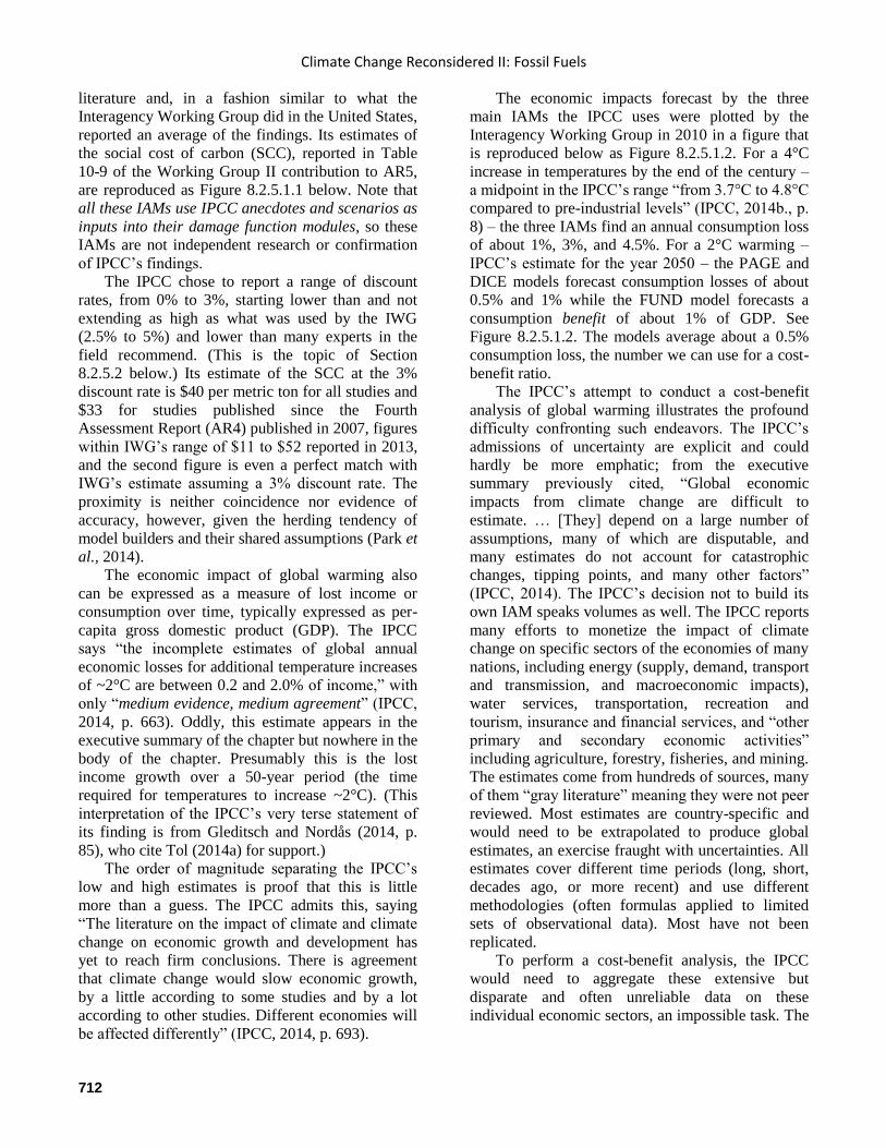
Climate Change Reconsidered II: Fossil Fuels

712

literature and, in a fashion similar to what the

Interagency Working Group did in the United States,

reported an average of the findings. Its estimates of

the social cost of carbon (SCC), reported in Table

10-9 of the Working Group II contribution to AR5,

are reproduced as Figure 8.2.5.1.1 below. Note that

all these IAMs use IPCC anecdotes and scenarios as

inputs into their damage function modules, so these

IAMs are not independent research or confirmation

of IPCC’s findings.

The IPCC chose to report a range of discount

rates, from 0% to 3%, starting lower than and not

extending as high as what was used by the IWG

(2.5% to 5%) and lower than many experts in the

field recommend. (This is the topic of Section

8.2.5.2 below.) Its estimate of the SCC at the 3%

discount rate is $40 per metric ton for all studies and

$33 for studies published since the Fourth

Assessment Report (AR4) published in 2007, figures

within IWG’s range of $11 to $52 reported in 2013,

and the second figure is even a perfect match with

IWG’s estimate assuming a 3% discount rate. The

proximity is neither coincidence nor evidence of

accuracy, however, given the herding tendency of

model builders and their shared assumptions (Park et

al., 2014).

The economic impact of global warming also

can be expressed as a measure of lost income or

consumption over time, typically expressed as per-

capita gross domestic product (GDP). The IPCC

says “the incomplete estimates of global annual

economic losses for additional temperature increases

of ~2°C are between 0.2 and 2.0% of income,” with

only “medium evidence, medium agreement” (IPCC,

2014, p. 663). Oddly, this estimate appears in the

executive summary of the chapter but nowhere in the

body of the chapter. Presumably this is the lost

income growth over a 50-year period (the time

required for temperatures to increase ~2°C). (This

interpretation of the IPCC’s very terse statement of

its finding is from Gleditsch and Nordås (2014, p.

85), who cite Tol (2014a) for support.)

The order of magnitude separating the IPCC’s

low and high estimates is proof that this is little

more than a guess. The IPCC admits this, saying

“The literature on the impact of climate and climate

change on economic growth and development has

yet to reach firm conclusions. There is agreement

that climate change would slow economic growth,

by a little according to some studies and by a lot

according to other studies. Different economies will

be affected differently” (IPCC, 2014, p. 693).

The economic impacts forecast by the three

main IAMs the IPCC uses were plotted by the

Interagency Working Group in 2010 in a figure that

is reproduced below as Figure 8.2.5.1.2. For a 4°C

increase in temperatures by the end of the century –

a midpoint in the IPCC’s range “from 3.7°C to 4.8°C

compared to pre-industrial levels” (IPCC, 2014b., p.

8) – the three IAMs find an annual consumption loss

of about 1%, 3%, and 4.5%. For a 2°C warming –

IPCC’s estimate for the year 2050 – the PAGE and

DICE models forecast consumption losses of about

0.5% and 1% while the FUND model forecasts a

consumption benefit of about 1% of GDP. See

Figure 8.2.5.1.2. The models average about a 0.5%

consumption loss, the number we can use for a cost-

benefit ratio.

The IPCC’s attempt to conduct a cost-benefit

analysis of global warming illustrates the profound

difficulty confronting such endeavors. The IPCC’s

admissions of uncertainty are explicit and could

hardly be more emphatic; from the executive

summary previously cited, “Global economic

impacts from climate change are difficult to

estimate. … [They] depend on a large number of

assumptions, many of which are disputable, and

many estimates do not account for catastrophic

changes, tipping points, and many other factors”

(IPCC, 2014). The IPCC’s decision not to build its

own IAM speaks volumes as well. The IPCC reports

many efforts to monetize the impact of climate

change on specific sectors of the economies of many

nations, including energy (supply, demand, transport

and transmission, and macroeconomic impacts),

water services, transportation, recreation and

tourism, insurance and financial services, and “other

primary and secondary economic activities”

including agriculture, forestry, fisheries, and mining.

The estimates come from hundreds of sources, many

of them “gray literature” meaning they were not peer

reviewed. Most estimates are country-specific and

would need to be extrapolated to produce global

estimates, an exercise fraught with uncertainties. All

estimates cover different time periods (long, short,

decades ago, or more recent) and use different

methodologies (often formulas applied to limited

sets of observational data). Most have not been

replicated.

To perform a cost-benefit analysis, the IPCC

would need to aggregate these extensive but

disparate and often unreliable data on these

individual economic sectors, an impossible task. The

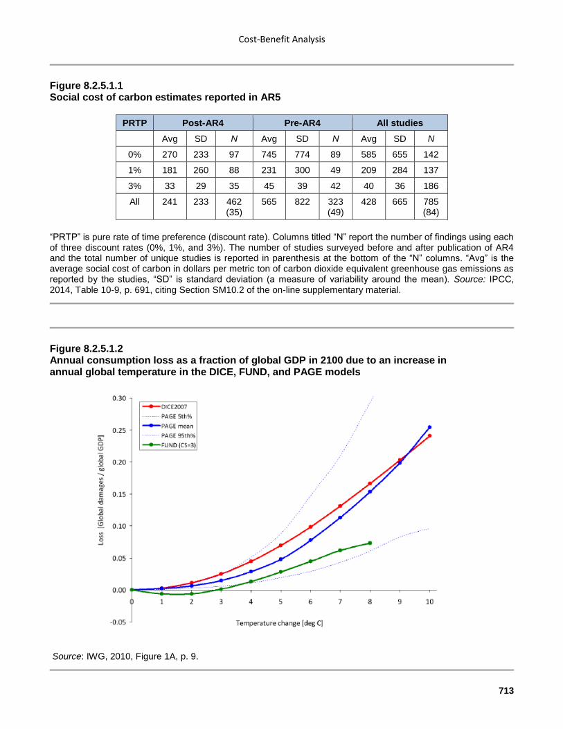
Cost-Benefit Analysis

713

Figure 8.2.5.1.1 Social cost of carbon estimates reported in AR5

PRTP Post-AR4 Pre-AR4 All studies

Avg SD N Avg SD N Avg SD N

0% 270 233 97 745 774 89 585 655 142

1% 181 260 88 231 300 49 209 284 137

3% 33 29 35 45 39 42 40 36 186

All 241 233 462 (35)

565 822 323 (49)

428 665 785 (84)

“PRTP” is pure rate of time preference (discount rate). Columns titled “N” report the number of findings using each of three discount rates (0%, 1%, and 3%). The number of studies surveyed before and after publication of AR4 and the total number of unique studies is reported in parenthesis at the bottom of the “N” columns. “Avg” is the average social cost of carbon in dollars per metric ton of carbon dioxide equivalent greenhouse gas emissions as reported by the studies, “SD” is standard deviation (a measure of variability around the mean). Source: IPCC, 2014, Table 10-9, p. 691, citing Section SM10.2 of the on-line supplementary material.

Figure 8.2.5.1.2 Annual consumption loss as a fraction of global GDP in 2100 due to an increase in annual global temperature in the DICE, FUND, and PAGE models

Source: IWG, 2010, Figure 1A, p. 9.

Climate Change Reconsidered II: Fossil Fuels

714

insurmountable problems it would have faced did

not disappear when it decided to rely on IAMs

created by others. The DICE, PAGE, and FUND

modelers faced the same challenges but went ahead

and produced unreliable estimates anyway.

Averaging the results of multiple IAMs does not

raise the probability of finding an SCC estimate or

impact on economic growth that is accurate. As

Frank observed, “systematic error does not average

away with repeated measurements. Repetition can

even increase error. When systematic error cannot be

eliminated and is known to be present, uncertainty

statements must be reported along with the data”

(Frank, 2016, p. 338).

In a review of IAMs, Warren et al. (2006)

concluded, “The assumption of a quadratic

dependence of damage on temperature rise is even

less grounded in any empirical evidence. Our review

of the literature uncovered no rationale, whether

empirical or theoretical, for adopting a quadratic

form for the damage function – although the practice

is endemic in IAMs.” Similarly, Pindyck has

lamented,

IAM damage functions are completely made

up, with no theoretical or empirical

foundation. They simply reflect common

beliefs (which might be wrong) regarding

the impact of 2°C or 3°C of warming, and

can tell us nothing about what might happen

if the temperature increases by 5°C or more.

And yet those damage functions are taken

seriously when IAMs are used to analyze

climate policy (Pindyck, 2013a, p. 16).

Also troubling is that these functions are usually

based on only one country or region because the

literature on the topic of environmentally induced

costs is very limited, except in agriculture. For

example, as described by Mastrandrea (2009):

Market and non‐market damages in DICE

are based on studies of impacts on the

United States that are then scaled up or

down for application to other regions. Many

of the estimates to which market damages in

PAGE are calibrated are also based on an

extrapolation of studies of the United States.

Only FUND uses regional and sector‐specific estimates. However, in some sectors

these estimates also originate in one country,

or may be dominated by estimates from one

region. For example, in the energy sector,

the sector which accounts for most of the

economic damages in FUND, estimates for

the UK are scaled across the world.

Summing up the cumulative effects of the many

shortcomings that prevent IAMs from being able to

accurately determine the economic impacts of

climate change, Pindyck writes:

… the greatest area of uncertainty concerns

the economic impact (including health and

social impacts) of climate change. The

economic loss functions that are part of most

IAMs are essentially ad hoc. This is not

surprising given how little we know – in

terms of both theory and data – about the

ways and extent to which changes in

temperature and other climate variables are

likely to affect the economy. In fact, the

economic impact of climate change may

well be in the realm of the “unknowable.”

This in turn means that IAM-based analyses

of climate change may not take us very far,

and the models may be of very limited use

as a policy tool (Pindyck, 2013b, p. 17).

Assuming arguendo that the IPCC’s estimate of

the economic impacts of global warming in 50 or

100 years is accurate, how should it be interpreted?

The IPCC’s estimate of the impact of a surface

temperature increase of ~2°C (from pre-industrial

levels), a loss of 1% of GDP around the year 2050,

is less than the expected global economic growth

rate in about four months. A single recession, even a

very short and mild recession, would have a larger

impact, and several are likely to occur before 2050.

Other than their choice of a low discount rate,

the authors of Chapter 10 of Working Group II’s

contribution to AR5 may be out-of-step with the

rhetoric and tone of other chapters of the WGII

contribution to AR5, but that is a good thing. While

the authors of other chapters seemed to think it their

duty to compile anecdotes of human suffering due to

extreme weather and natural disasters and to

speculate that such events will become more

frequent in the future due to human interference in

the climate, the authors of Chapter 10 took more

seriously their duty to prove the links in the logical

chain behind such claims (even while accepting the

IPCC’s distorted views in the emission scenarios and

carbon cycle modules), and then to monetize the

harms.

Cost-Benefit Analysis

715

One of the two lead authors of Chapter 10,

Richard S.J. Tol, is the creator of the FUND model,

one of the three IAMs most prominent in the climate

change literature. Significantly, Tol resigned from

the IPCC shortly before AR5 was released. He

explained why in a blogpost on April 25, 2014:

In the earlier drafts of the SPM, there was a

key message that was new, snappy and

relevant: Many of the more worrying

impacts of climate change really are

symptoms of mismanagement and under-

development. This message does not

support the political agenda for greenhouse

gas emission reduction. Later drafts put

more and more emphasis on the reasons for

concern about climate change, a concept I

had helped to develop for AR3. Raising the

alarm about climate change has been tried

before, many times in fact, but it has not had

an appreciable effect on greenhouse gas

emissions. I reckoned that putting my name

on such a document would not be credible –

my opinions are well-known – and I

withdrew (Tol, 2014b, boldface in original).

Economics, as explained in Chapter 1, uses data

about prices and investment returns to make

objective what are otherwise only subjective

impressions, preferences, and anecdotes. When

applied to the impacts of climate change, economics

can reveal the true net costs of climate change,

should it occur and provided the data that enter

earlier modules in the IAMs are accurate. Even with

the IPCC’s thumb on the scale in this respect, it is

remarkable to see how small the economic

consequences of climate change would be.

References

BBC. 2014. Fossil fuels should be “phased out by 2100”

says IPCC. November 2. Accessed November 17, 2018.

Frank, P. 2016. Systematic error in climate

measurements: the surface air temperature record.

International Seminars on Nuclear War and Planetary

Emergencies 48th Session. Presentation in Erice, Italy on

August 19–25, pp. 337–51.

Gillis, J. 2014. UN panel issues its starkest warning yet on

global warming. The New York Times, November 2.

Accessed November 17, 2018.

Gleditsch, N.P. and Nordås, R. 2014. Conflicting

messages? The IPCC on conflict and human security.

Political Geography 43: 82–90.

IPCC. 2014. Intergovernmental Panel on Climate Change.

Climate Change 2014: Impacts, Adaptation, and

Vulnerability. Part A: Global and Sectoral Aspects.

Contribution of Working Group II to the Fifth Assessment

Report of the Intergovernmental Panel on Climate

Change. New York, NY: Cambridge University Press.

IWG. 2010. Interagency Working Group on the Social

Cost of Carbon. Technical Support Document: Social

Cost of Carbon for Regulatory Impact Analysis Under

Executive Order 12866. Washington, DC. February.

Mastrandrea, M.D. 2009. Calculating the Benefits of

Climate Policy: Examining the Assumptions of Integrated

Assessment Models. Arlington, VA: The Pew Center on

Global Climate Change.

Park, I.-U., Peacey, M.W., and Munafo, M.R. 2014.

Modelling the effects of subjective and objective decision

making in scientific peer review. Nature 506 (7486): 93–

6.

Pindyck, R.S. 2013a. Climate change policy: what do the

models tell us? Journal of Economic Literature 51: 860–

72.

Pindyck, R.S. 2013b. The climate policy dilemma. Review

of Environmental Economics and Policy 7: 219–37.

Reuters. 2014. Threat from global warming heightened in

latest U.N. report. March 31. Accessed on November 17,

2018.

Tol, R.S.J. 2014a. Bogus prophecies of doom will not fix

the climate. Financial Times. March 31.

Tol, R.S.J. 2014b. IPCC again. Richard Tol Occasional

thoughts on all sorts (blog). Accessed June 26, 2018.

Warren, R., Hope, C., Mastrandrea, M., Tol, R.S.J.,

Adger, N., and Lorenzoni, I. 2006. Spotlighting impacts

functions in integrated assessment. Research Report

Prepared for the Stern Review on the Economics of

Climate Change. Tyndall Centre for Climate Change

Research. Working Paper 91. September.

8.2.5.2 Discount Rates

As discussed in Chapter 1, Section 1.2.8, the

selection of a discount rate (referred to in the U.K. as

the “social time preference rate” or STPR) is one of

the most controversial issues in the climate change

debate (Heal and Millner, 2014; Weitzman, 2015).

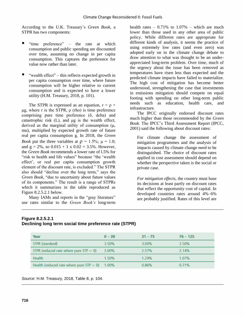
Climate Change Reconsidered II: Fossil Fuels

716

According to the U.K. Treasury’s Green Book, a

STPR has two components:

“time preference” – the rate at which

consumption and public spending are discounted

over time, assuming no change in per capita

consumption. This captures the preference for

value now rather than later.

“wealth effect” – this reflects expected growth in

per capita consumption over time, where future

consumption will be higher relative to current

consumption and is expected to have a lower

utility (H.M. Treasury, 2018, p. 101).

The STPR is expressed as an equation, r = ρ +

μg, where r is the STPR, ρ (rho) is time preference

comprising pure time preference (δ, delta) and

catastrophic risk (L), and μg is the wealth effect,

derived as the marginal utility of consumption (μ,

mu), multiplied by expected growth rate of future

real per capita consumption g. In 2018, the Green

Book put the three variables at ρ = 1.5%; μ = 1.0;

and g = 2%, so 0.015 + 1 x 0.02 = 3.5%. However,

the Green Book recommends a lower rate of l.5% for

“risk to health and life values” because “the ‘wealth

effect’, or real per capita consumption growth

element of the discount rate, is excluded.” The STPR

also should “decline over the long term,” says the

Green Book, “due to uncertainty about future values

of its components.” The result is a range of STPRs

which it summarizes in the table reproduced as

Figure 8.2.5.2.1 below.

Many IAMs and reports in the “gray literature”

use rates similar to the Green Book’s long-term

health rates – 0.71% to 1.07% – which are much

lower than those used in any other area of public

policy. While different rates are appropriate for

different kinds of analysis, it seems the practice of

using extremely low rates (and even zero) was

adopted early on in the climate change debate to

draw attention to what was thought to be an under-

appreciated long-term problem. Over time, much of

the urgency about the issue has been removed as

temperatures have risen less than expected and the

predicted climate impacts have failed to materialize.

The high cost of mitigation has become better

understood, strengthening the case that investments

in emissions mitigation should compete on equal

footing with spending on other long-term public

needs such as education, health care, and

infrastructure.

The IPCC originally endorsed discount rates

much higher than those recommended by the Green

Book. The IPCC’s Third Assessment Report (IPCC,

2001) said the following about discount rates:

For climate change the assessment of

mitigation programmes and the analysis of

impacts caused by climate change need to be

distinguished. The choice of discount rates

applied in cost assessment should depend on

whether the perspective taken is the social or

private case.

For mitigation effects, the country must base

its decisions at least partly on discount rates

that reflect the opportunity cost of capital. In

developed countries rates around 4%–6%

are probably justified. Rates of this level are

Figure 8.2.5.2.1 Declining long term social time preference rate (STPR)

Source: H.M. Treasury, 2018, Table 8, p. 104.

Cost-Benefit Analysis

717

in fact used for the appraisal of public sector

projects in the European Union (EU) (Watts,

1999). In developing countries the rate could

be as high as 10%–12%. The international

banks use these rates, for example, in

appraising investment projects in developing

countries. It is more of a challenge, therefore,

to argue that climate change mitigation

projects should face different rates, unless the

mitigation project is of very long duration.

These rates do not reflect private rates of

return, which typically need to be

considerably higher to justify the project,

potentially between 10% and 25%.

For climate change impacts, the long-term

nature of the problem is the key issue. The

benefits of reduced [greenhouse gas (GHG)]

emissions vary with the time of emissions

reduction, with the atmospheric GHG

concentration at the reduction time, and with

the total GHG concentrations more than 100

years after the emissions reduction. Any

“realistic” discount rate used to discount the

impacts of increased climate change impacts

would render the damages, which occur over

long periods of time, very small. With a

horizon of around 200 years, a discount rate

of 4% implies that damages of USD1 at the

end of the period are valued at 0.04 cents

today. At 8% the same damages are worth

0.00002 cents today. Hence, at discount rates

in this range the damages associated with

climate change become very small and even

disappear (Cline, 1993)” (IPCC, 2001, p.

466).

There are two main points to be taken from this

passage. First, investments in mitigation should be

held to the same standard as other investments, public

or private, to ensure capital flows to its highest and

best use. For developing countries, the IPCC suggests

using discount rates as high as 10% to 12%. Second,

“the range of dangers associated with climate change

become very small and even disappear” as the chosen

discount rate increases. It should therefore come as

no surprise that governments and other proponents of

immediate action to slow or stop climate change

favor the use of lower discount rates. At higher (and

likely more appropriate) discount rates, there is no

economic rationale for immediate action.

In 2001, the IPCC cited a survey by Weitzman

(1998) of 1,700 professional economists suggesting

they believe “lower rates should be applied to

problems with long time horizons, such as that being

discussed here,” and Weitzman “suggests the

appropriate discount rate for long-lived projects is

less than 2%” (IPCC, 2001, p. 467). In the eyes of

some, discounting at all is unethical (Broome, 2004,

2012; Heal, 2009; Stern, 2014). They claim it violates

intergenerational neutrality, causing future

generations to be held as less valuable than the

current one. But this logic seems flawed since the

cost of reducing greenhouse gas emissions to benefit

future generations must be compared to other

investments that would also benefit future

generations. Nearly any investment in capital and

services that raises productivity and produces wealth

will benefit future generations.

Weitzman (2007) and a team of other economists

(Arrow et al., 2013) have sided with a declining

discount rate based on a formula called the Ramsey

discounting formula, in which benefits realized in the

immediate future (one to five years) might be

discounted at 4%, those in the medium future (26–75

years) at 2%, and those in the distant future (76–300

years) at 1%. But once again, this seems counter-

intuitive. Making investments in emission reductions

that yield less than the return on alternative

investments impoverishes future generations

(Birdsall and Steer, 1993; Klaus, 2012). As Robert

Mendelsohn wrote in 2004, “if climate change can

only earn a 1.5% return each year, there are many

more deserving social activities that we must fund

before we get to climate. Although climate impacts

are long term, that does not justify using a different

price for time” (Mendelsohn, 2004).

Other economists argue for discount rates higher

than the Ramsey formula. Carter et al. wrote,

“because our knowledge of future events becomes

more uncertain as the time horizon is extended,

discount rates should if anything increase rather than

diminish with time” (Carter et al., 2006). The passage

of time diminishes the odds that any specific event,

whether harmful (cost) or desirable (benefit), will

come to pass. It is therefore logical to discount the

possibility of ever seeing a benefit whose delivery is

decades or even a century distant. In the climate

debate, delivery of the benefit can be foiled by even

small changes in population, consumption,

technology, politics, and international affairs that can

(following the IPCC’s chain of logic) change

emission scenarios, hence atmospheric concentrations

Climate Change Reconsidered II: Fossil Fuels

718

of CO2, hence climate impacts, and hence economic

impacts.

Another reason to believe discount rates should

be high rather than low for benefits realized in the far

future is because future generations will be much

wealthier than people are today and therefore better

able to cope with the risks that might accompany

climate change. “There is a general consensus among

economists that future generations will be able to

deal with the average impacts of climate change

relatively uneventfully,” writes Litterman (2013, p.

38). At an annual per-capita income growth rate of

2.8% (the average over the past 50 years), average

personal income will be four times as high as today

in 50 years and 16 times as high in 100 years. In the

latter case, even the world’s poor will be wealthier

than middle-income wage earners today, giving them

access to mobility, air conditioning, and other forms

of adaptation to climate hazards that currently may be

beyond their reach (Goklany, 2009).

Nigel Lawson reports the rate the British

Treasury set for public-sector projects was 6% during

his time as U.K. Chancellor, and he is skeptical of the

justification for a subsequent reduction to 3.5%,

pointing out the private-sector rate is considerably

higher (Lawson, 2008, p. 84). The issue, he observes,

is not what would be an appropriate rate for

developed countries, but what rate should be applied

to a global project, and as the IPCC admits in the

excerpt above, normal rates in developing countries

are considerably higher.

The U.S. Office of Management and Budget

(OMB) guidelines for base-line analysis state,

“Constant-dollar benefit-cost analyses of proposed

investments and regulations should report net present

value and other outcomes determined using a real

discount rate of 7%. This rate approximates the

marginal pretax rate of return on an average

investment in the private sector in recent years”

(OMB, 1992, p. 9). Another commonly referenced

benchmark is the return on U.S. Treasury notes,

which at the time of this writing was 3.14%

(Bankrates.com, 2018).

Economists generally reject the notion that

climate change should be singled out for unique

treatment, arguing the assessment of present values

of future benefits/costs rests on principles that are

rational and immutable (e.g., Mendelsohn, 2004).

Although expenditures can be viewed very

differently in terms of diverse politics, moral

philosophy, or ethics, they contend discount rates

used for inter-temporal calculations should be around

the real rate of return on capital, because only that

rate represents the true opportunity cost of

investments in climate mitigation (Nordhaus, 1998;

Murphy, 2008). According to Kreutzer (2016),

What, then, is the best reasonable return on

investment? While one cannot predict what

future rates will be, past rates of return on

broad indexes are an excellent guide. The

return on the Standard & Poor’s 500 from

1928 to 2014 was 9.60 percent. Over this

time inflation was a compounded 3.1 percent.

The real rate of return would be the

difference, 6.5 percent per year. Another

source estimates the return for all stocks in

the U.S. from 1802 to 2002 and gets the same

6.5 percent real return on capital. Yet another

source calculates the real return on stocks

between 1802 and 2002 to be 6.8 percent per

year. These estimates reflect the returns after

corporate income taxes are paid. Adjusting

for corporate profits taxes increases these

rates to between 7.5 percent and 9.9 percent.

Kreutzer concludes, “In any event, the 7 percent

discount rate that is part of the Office of Management

and Budget’s guidance does not seem too high”

(Ibid.).

The exception that seems to draw many

researchers away from this consensus is Sir Nicholas

Stern, whose 2007 Stern Review based its analysis on

a discount rate of roughly 1.4% or even as low as

0.1% (Stern, 2007; Stern Review team, 2006). Stern

justifies his rate as follows:

The most straightforward and defensible

interpretation (as argued in the Review) of

[the utility discount factor] δ is the

probability of existence of the world. In the

Review, we took as our base case δ =

0.1%/year, which gives roughly a one-in-ten

chance of the planet not seeing out this

century. [Annual per-capita consumption

growth] is on average ~1.3% in a world

without climate change, giving an average

consumption or social discount rate across

the entire period of 1.4% (being lower where

the impacts of climate change depress

consumption growth) (Dietz et al., 2007).

Stern assumes a one-in-ten probability that

anthropogenic global warming will bring the world to

an end by 2100, the social discount rate would indeed

be vanishingly different from zero. But that

Cost-Benefit Analysis

719

doomsday scenario defies logic as well as climate

science and economics. Carbon dioxide’s effect on

climate and then climate change’s effect on human

well-being are likely to be small relative to other

human needs and priorities, even well past the end of

the twenty-first century. Investing in efforts to

mitigate their effects ought not be raised above other

needs without sound scientific and economic

justification. Stern’s focus on an utterly implausible

scenario makes his advice on a discount rate

unreliable.

The detailed analyses of the risk of

anthropogenic climate change presented earlier in

this chapter and in previous chapters make a strong

case that there is nothing special or unique about

climate change that would justify an exceptional

discount rate. Estimates of future costs and benefits

and investments in emission reductions should be

discounted at the same rate as other costs, benefits,

and investment opportunities that face similar

uncertainties. Special pleading or exception-making

opens the door for bad public policy choices, thereby

undermining the goals of CBA in the first place.

Finding the right discount rate has major

consequences for estimating the human welfare

impacts of climate change. The debate over choosing

an appropriate discount rate is certainly worth

having, but opponents of using a constant discount

rate of approximately 7%, as recommended by OMB,

Kreutzer, and others, have a tough position to defend.

References

Arrow, K.J., et al. 2013. How should benefits and costs be

discounted in an intergenerational context? Economics

Department Working Paper Series No. 56-2013.

Colchester, UK: University of Essex, Business,

Management, and Economics.

Bankrates.com. 2018. Ten-year Treasury constant maturity

(website). Accessed November 17, 2018.

Birdsall, N. and Steer, A. 1993. Act now on global

warming – but don’t cook the books. Finance and

Development 30 (1): 6–8.

Broome, J. 2004. Weighing Lives. Oxford, UK: Oxford

University Press.

Broome, J. 2012. Climate Matters: Ethics in a Warming

World. New York, NY: W.W. Norton & Company.

Carter, R.M., et al. 2006. The Stern Review: A dual

critique. World Economics 7 (4).

Cline, W.M. 1993. Give greenhouse abatement a chance.

Finance and Development. March.

Dietz, S., Hope, C., Stern, N., and Zenghelis, D. 2007.

Reflections on the Stern Review (1): a robust case for

strong action to reduce the risks of climate change. World

Economics 8 (1): 121–68.

Goklany, I.M. 2009. Discounting the future. Regulation 32

(1): 37–40.

Heal, G. 2009. Climate economics: a meta-review and

some suggestions. Review of Environmental Economics

and Policy 3: 4–21.

Heal, G.M. and Millner, A. 2014. Agreeing to disagree on

climate policy. Proceedings of the National Academy of

Sciences USA 111: 3695–8.

H.M. Treasury. 2018. Green Book: Central Governance

Guidance on Appraisal and Evaluation. London, UK.

IPCC. 2001. Intergovernmental Panel on Climate Change.

Climate Change 2001: Mitigation. Report of Working

Group III to the Third Assessment Report of the

Intergovernmental Panel on Climate Change. New York,

NY: Cambridge University Press.

Klaus, V. 2012. Magistral Lecture on Climate Economics,

45th Annual Seminars on Planetary Emergencies. World

Federation of Scientists, Erice, Sicily. Washington, DC:

Science and Public Policy Institute.

Kreutzer, D. 2016. Discounting climate costs. The

Heritage Foundation (website). Accessed July 19, 2018.

Lawson, N. 2008. An Appeal to Reason: A Cool Look at

Global Warming. New York, NY: Overlook.

Litterman, B. 2013. What is the right price for carbon

emissions? Regulation 36 (2): 38–42.

Mendelsohn, R. 2004. The challenge of global warming.

Opponent paper on climate change. In: Lomborg, B. (Ed.)

Global Crises, Global Solutions. Cambridge, MA:

Cambridge University Press.

Murphy, K.M. 2008. Some Simple Economics of Climate

Changes. Paper presented to the Mont Pelerin Society

General Meeting, Tokyo. September 8.

Nordhaus, W.D. 1998. Economics and Policy Issues in

Climate Change. Washington, DC: Resources for the

Future.

OMB. 1992. U.S. Office of Management and Budget.

Circular A-94 Guidelines and discount rates for benefit-

cost analysis of federal programs. Washington, DC.

Climate Change Reconsidered II: Fossil Fuels

720

Stern, N. 2007. The Economics of Climate Change: The

Stern Review. Cambridge, UK: Cambridge University

Press.

Stern, N. 2014. Ethics, equity and the economics of

climate change paper 1: science and philosophy.

Economics and Philosophy 30: 397–444.

Stern Review Team. 2006. Personal communication to

Christopher Monckton of Brenchley.

Tol, R.S.J. 2010. Carbon dioxide mitigation. In: Lomborg,

B. (Ed.) Smart Solutions to Climate Change: Comparing

Costs and Benefits. New York, NY: Cambridge University

Press, pp. 74–105.

Watts, W. 1999. Discounting and Sustainability. Brussels,

Belgium: The European Commission, Directorate General

of Democracy.

Weitzman, M.L. 1998. Why the far-distant future should

be discounted at its lowest possible rate. Journal of

Environmental Economics and Management 36: 201–8.

Weitzman, M.L. 2007. A review of the Stern Review on

the Economics of Climate Change. Journal of Economic

Literature XLV (September).

Weitzman, M.L. 2015. A review of William Nordhaus’

The Climate Casino: Risk, Uncertainty, and Economics for

a Warming World. Review of Environmental Economics

and Policy 9: 145–56.

8.3 Climate Change

Previous sections of this chapter have shown how

cascading uncertainty cripples integrated assessment

models (IAMs). All five steps in an IAM – emission

scenarios, carbon cycle, climate sensitivity, climate

impacts, and economic impacts – rely on assumptions

and controversial assertions that undermine the

credibility of these academic exercises. They are, as

Pindyck (2013) wrote, “close to useless as tools for

policy analysis.”

Assuming arguendo that IAMs get some aspects

of the climate change problem right, this section

begins with a summary of what the IPCC in its Fifth

Assessment Report says the models show. It is

seldom noted that the IPCC’s estimates of the cost of

reducing greenhouse gas emissions is reported in the

Working Group III report while the benefits appear in

the Working Group II report. What happens when

those two estimates are compared? Section 8.3.1

answers that question.

Sections 8.3.2 and 8.3.3 report what happened

when Dayaratna et al. (2017) re-ran two of the three

IAMs relied upon by the IPCC to estimate the “social

cost of carbon” using different assumptions regarding

climate sensitivity, discount rates, and number of

years being forecast. (The researchers also were

interested in examining the robustness of the IPCC’s

third model, the PAGE model (Hope, 2013, 2018),

but the author of that model, Chris Hope, insisted on

co-authorship of any publications that would be

written in exchange for providing his codes, so that

model was not studied.)

References

Dayaratna, K., McKitrick, R., and Kreutzer, D. 2017.

Empirically-constrained climate sensitivity and the social

cost of carbon. Climate Change Economics 8: 2.

Doiron, H.H. 2016. Recommendations to the Trump

Transition Team Investigating Actions to Take at the

Environmental Protection Agency (EPA): A Report of The

Right Climate Stuff Research Team. November 30, p. 20.

Hope, C.W. 2013. Critical issues for the calculation of the

social cost of CO2: why the estimates from PAGE09 are

higher than those from PAGE2002. Climatic Change 117:

531–43.

Hope, C.W. 2018. PAGE. Climate Colab (website).

Accessed July 19, 2018.

Pindyck, R.S. 2013. Climate change policy: what do the

models tell us? Journal of Economic Literature 51: 860–

72.

8.3.1 The IPCC’s Findings

By the IPCC’s own estimates, the cost of

reducing emissions in 2050 by enough to

avoid a warming of ~2°C would be 6.8 times

as much as the benefits would be worth.

The IPCC’s estimate of the economic impact of

unmitigated climate change was discussed in some

detail in Section 8.2.5.1. Working Group II’s

contribution to AR5 put the cost of unmitigated

climate change at between 0.2% and 2.0% of annual

global GDP for a warming of approximately 2°C by

2050 (IPCC, 2014a, p. 663). Presumably this is the

lost income growth over a 50-year period (the time

required for temperatures to increase ~2°C)

(Gleditsch and Nordås, 2014, p. 85). A mean cost

Cost-Benefit Analysis

721

estimate might be 1% (2.2 / 2), but this is higher than

what the IPCC’s IAMs forecast (see Figure

8.2.5.1.2). For a 2°C warming the PAGE and DICE

models forecast consumption losses of about 0.5%

and 1% while the FUND model forecasts a

consumption benefit of about 1% of GDP. The

models average about a 0.5% consumption loss.

Avoiding this cost would be the benefit of reducing

emissions sufficiently to keep the warming from

occurring.

The Working Group III contribution to AR5 puts

the cost of reducing greenhouse gas emissions

enough to avoid more than 2°C warming by 2100 at

1.7% of global GDP in 2030, 3.4% in 2050, and 4.8%

in 2100 (IPCC, 2014b, Table SPM.2, p. 15). These

are “global mitigation costs” discounted at 5% per

year and do not include the possible benefits or costs

of climate impacts.

Working Group III says without mitigation,

“global mean surface temperature increases in 2100

from 3.7°C to 4.8°C compared to pre-industrial

levels” (IPCC, 2014b, p. 8). But Working Group II

doesn’t offer an estimate of the cost of unmitigated

climate change much higher than ~2°C, saying

“losses accelerate with greater warming (limited

evidence, high agreement), but few quantitative

estimates have been completed for additional

warming around 3°C or above. … Estimates vary

strongly with the assumed damage function and

discount rate” (IPCC, 2014a, p. 663). On this point

we can agree with the IPCC: Accurately forecasting

economic costs and benefits more than 40 or 50 years

distant is impossible.

The ratio of the IPCC’s estimates of the costs and

benefits of reducing emissions sufficiently to prevent

more than 2°C warming by 2050 is 6.8:1 (3.4/0.5).

This seems as close to a cost-benefit ratio as one can

derive from the IPCC’s voluminous research and

commentary on impacts and mitigation. Reducing

emissions would cost approximately seven times as

much as any possible benefits that might come from a

slightly cooler world in 2050 and beyond. This means

the IPCC itself makes a strong case against reducing

emissions before 2050. But given all the errors in the

IPCC’s analysis documented in this and earlier

chapters, a better cost-benefit ratio is in order.

References

Gleditsch, N.P. and Nordås, R. 2014. Conflicting

messages? The IPCC on conflict and human security.

Political Geography 43: 82–90.

IPCC. 2014a. Intergovernmental Panel on Climate Change.

Climate Change 2014: Impacts, Adaptation, and

Vulnerability. Part A: Global and Sectoral Aspects.

Contribution of Working Group II to the Fifth Assessment

Report of the Intergovernmental Panel on Climate Change.

New York, NY: Cambridge University Press.

IPCC. 2014b. Intergovernmental Panel on Climate

Change. Climate Change 2014: Mitigation of Climate

Change. Contribution of Working Group III to the Fifth

Assessment Report of the Intergovernmental Panel on

Climate Change. New York, NY: Cambridge University

Press.

8.3.2 DICE and FUND Models

Changing only three assumptions in two

leading IAMs – the DICE and FUND models

– reduces the SCC by an order of magnitude

for the first and changes the sign from

positive to negative for the second.

The two publicly available models used by the U.S.

Interagency Working Group (IWG) for policymaking

prior to 2017 were the Dynamic Integrated Climate-

Economy (DICE) model (Newbold, 2010; Nordhaus,

2017), and the Climate Framework for Uncertainty,

Negotiation and Distribution (FUND) model

(Anthoff and Tol, 2014; Waldhoff et al., 2014; Tol

and Anthoff, 2018). Examination of the DICE and

FUND models by Dayaratna et al. (2017) revealed

they are especially sensitive to three parameters

chosen by IWG: discount rates, equilibrium climate

sensitivity, and the number of years being forecast.

IWG simply chose not to run the models with the 7%

discount rate required by the U.S. Office of

Management and Budget (OMB, 1992) and

recommended by many economists as recounted in

Section 8.2.5.2. So Dayaratna et al. ran the models

themselves. As previously mentioned, a third model,

PAGE, was not used due to the author’s insistence of

co-authorship, precluding independent analysis.

Equilibrium climate sensitivity (ECS) was

discussed in detail in Chapter 2 and in Section 8.2.3.

The ECS distribution used by IWG was published in

the journal Science 11 years ago (Roe and Baker,

2007). Rather than being based on empirical data,

this distribution was calibrated to assumptions made

by IWG. Since it was published, studies regarding

ECS distributions have found a significantly lower

probability of extreme global warming (see Figure

8.2.3.5 and Otto et al., 2013; Lewis, 2013; and Lewis

and Curry, 2015). Dayaratna et al. (2017) re-ran the

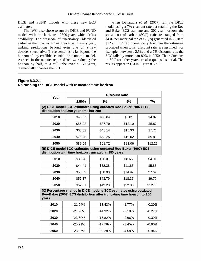
Climate Change Reconsidered II: Fossil Fuels

722

DICE and FUND models with these new ECS

estimates.

The IWG also chose to run the DICE and FUND

models with time horizons of 300 years, which defies

credibility. The “cascade of uncertainty” identified

earlier in this chapter grows greater with every year,

making predictions beyond even one or a few

decades speculative. Three centuries is far beyond the

horizon of any credible scientific or economic model.

As seen in the outputs reported below, reducing the

horizon by half, to a still-unbelievable 150 years,

dramatically changes the SCC.

When Dayaratna et al. (2017) ran the DICE

model using a 7% discount rate but retaining the Roe

and Baker ECS estimate and 300-year horizon, the

social cost of carbon (SCC) estimates ranged from

$4.02 per marginal ton of CO2eq generated in 2010 to

$12.25 in 2050, dramatically less than the estimates

produced when lower discount rates are assumed. For

example, between a 2.5% and a 7% discount rate, the

SCC falls by more than 80% in 2050. The reductions

in SCC for other years are also quite substantial. The

results appear in (A) in Figure 8.3.2.1.

Figure 8.3.2.1 Re-running the DICE model with truncated time horizon

Year Discount Rate

2.50% 3% 5% 7%

(A) DICE model SCC estimates using outdated Roe-Baker (2007) ECS distribution and 300 year time horizon

2010 $46.57 $30.04 $8.81 $4.02

2020 $56.92 $37.79 $12.10 $5.87

2030 $66.52 $45.14 $15.33 $7.70

2040 $76.95 $53.25 $19.02 $9.85

2050 $87.69 $61.72 $23.06 $12.25

(B) DICE model SCC estimates using outdated Roe-Baker (2007) ECS distribution with time horizon truncated at 150 years

2010 $36.78 $26.01 $8.66 $4.01

2020 $44.41 $32.38 $11.85 $5.85

2030 $50.82 $38.00 $14.92 $7.67

2040 $57.17 $43.79 $18.36 $9.79

2050 $62.81 $49.20 $22.00 $12.13

(C) Percentage change in DICE model’s SCC estimates using outdated Roe-Baker (2007) ECS distribution after truncating time horizon to 150 years

2010 -21.04% -13.43% -1.77% -0.20%

2020 -21.98% -14.32% -2.10% -0.27%

2030 -23.60% -15.82% -2.66% -0.39%

2040 -25.71% -17.78% -3.45% -0.60%

2050 -28.37% -20.28% -4.58% -0.94%

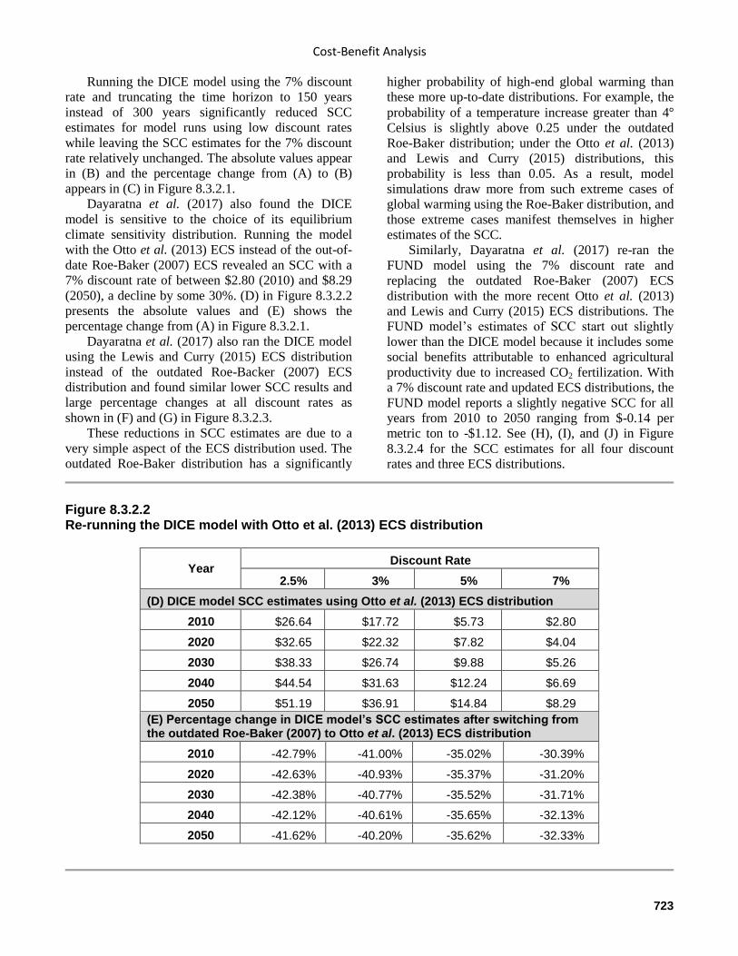
Cost-Benefit Analysis

723

Running the DICE model using the 7% discount

rate and truncating the time horizon to 150 years

instead of 300 years significantly reduced SCC

estimates for model runs using low discount rates

while leaving the SCC estimates for the 7% discount

rate relatively unchanged. The absolute values appear

in (B) and the percentage change from (A) to (B)

appears in (C) in Figure 8.3.2.1.

Dayaratna et al. (2017) also found the DICE

model is sensitive to the choice of its equilibrium

climate sensitivity distribution. Running the model

with the Otto et al. (2013) ECS instead of the out-of-

date Roe-Baker (2007) ECS revealed an SCC with a

7% discount rate of between $2.80 (2010) and $8.29

(2050), a decline by some 30%. (D) in Figure 8.3.2.2

presents the absolute values and (E) shows the

percentage change from (A) in Figure 8.3.2.1.

Dayaratna et al. (2017) also ran the DICE model

using the Lewis and Curry (2015) ECS distribution

instead of the outdated Roe-Backer (2007) ECS

distribution and found similar lower SCC results and

large percentage changes at all discount rates as

shown in (F) and (G) in Figure 8.3.2.3.

These reductions in SCC estimates are due to a

very simple aspect of the ECS distribution used. The

outdated Roe-Baker distribution has a significantly

higher probability of high-end global warming than

these more up-to-date distributions. For example, the

probability of a temperature increase greater than 4°

Celsius is slightly above 0.25 under the outdated

Roe-Baker distribution; under the Otto et al. (2013)

and Lewis and Curry (2015) distributions, this

probability is less than 0.05. As a result, model

simulations draw more from such extreme cases of

global warming using the Roe-Baker distribution, and

those extreme cases manifest themselves in higher

estimates of the SCC.

Similarly, Dayaratna et al. (2017) re-ran the

FUND model using the 7% discount rate and

replacing the outdated Roe-Baker (2007) ECS

distribution with the more recent Otto et al. (2013)

and Lewis and Curry (2015) ECS distributions. The

FUND model’s estimates of SCC start out slightly

lower than the DICE model because it includes some

social benefits attributable to enhanced agricultural

productivity due to increased CO2 fertilization. With

a 7% discount rate and updated ECS distributions, the

FUND model reports a slightly negative SCC for all

years from 2010 to 2050 ranging from $-0.14 per

metric ton to -$1.12. See (H), (I), and (J) in Figure

8.3.2.4 for the SCC estimates for all four discount

rates and three ECS distributions.

Figure 8.3.2.2 Re-running the DICE model with Otto et al. (2013) ECS distribution

Year Discount Rate

2.5% 3% 5% 7%

(D) DICE model SCC estimates using Otto et al. (2013) ECS distribution

2010 $26.64 $17.72 $5.73 $2.80

2020 $32.65 $22.32 $7.82 $4.04

2030 $38.33 $26.74 $9.88 $5.26

2040 $44.54 $31.63 $12.24 $6.69

2050 $51.19 $36.91 $14.84 $8.29

(E) Percentage change in DICE model’s SCC estimates after switching from the outdated Roe-Baker (2007) to Otto et al. (2013) ECS distribution

2010 -42.79% -41.00% -35.02% -30.39%

2020 -42.63% -40.93% -35.37% -31.20%

2030 -42.38% -40.77% -35.52% -31.71%

2040 -42.12% -40.61% -35.65% -32.13%

2050 -41.62% -40.20% -35.62% -32.33%

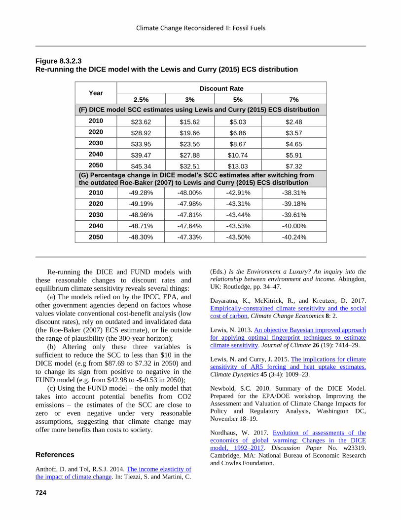
Climate Change Reconsidered II: Fossil Fuels

724

Figure 8.3.2.3 Re-running the DICE model with the Lewis and Curry (2015) ECS distribution

Year Discount Rate

2.5% 3% 5% 7%

(F) DICE model SCC estimates using Lewis and Curry (2015) ECS distribution

2010 $23.62 $15.62 $5.03 $2.48

2020 $28.92 $19.66 $6.86 $3.57

2030 $33.95 $23.56 $8.67 $4.65

2040 $39.47 $27.88 $10.74 $5.91

2050 $45.34 $32.51 $13.03 $7.32

(G) Percentage change in DICE model’s SCC estimates after switching from the outdated Roe-Baker (2007) to Lewis and Curry (2015) ECS distribution

2010 -49.28% -48.00% -42.91% -38.31%

2020 -49.19% -47.98% -43.31% -39.18%

2030 -48.96% -47.81% -43.44% -39.61%

2040 -48.71% -47.64% -43.53% -40.00%

2050 -48.30% -47.33% -43.50% -40.24%

Re-running the DICE and FUND models with

these reasonable changes to discount rates and

equilibrium climate sensitivity reveals several things:

(a) The models relied on by the IPCC, EPA, and

other government agencies depend on factors whose

values violate conventional cost-benefit analysis (low

discount rates), rely on outdated and invalidated data

(the Roe-Baker (2007) ECS estimate), or lie outside

the range of plausibility (the 300-year horizon);

(b) Altering only these three variables is

sufficient to reduce the SCC to less than $10 in the

DICE model (e.g from $87.69 to $7.32 in 2050) and

to change its sign from positive to negative in the

FUND model (e.g. from $42.98 to -$-0.53 in 2050);

(c) Using the FUND model – the only model that

takes into account potential benefits from CO2

emissions – the estimates of the SCC are close to

zero or even negative under very reasonable

assumptions, suggesting that climate change may

offer more benefits than costs to society.

References

Anthoff, D. and Tol, R.S.J. 2014. The income elasticity of

the impact of climate change. In: Tiezzi, S. and Martini, C.

(Eds.) Is the Environment a Luxury? An inquiry into the

relationship between environment and income. Abingdon,

UK: Routledge, pp. 34–47.

Dayaratna, K., McKitrick, R., and Kreutzer, D. 2017.

Empirically-constrained climate sensitivity and the social

cost of carbon. Climate Change Economics 8: 2.

Lewis, N. 2013. An objective Bayesian improved approach

for applying optimal fingerprint techniques to estimate

climate sensitivity. Journal of Climate 26 (19): 7414–29.

Lewis, N. and Curry, J. 2015. The implications for climate

sensitivity of AR5 forcing and heat uptake estimates.

Climate Dynamics 45 (3-4): 1009–23.

Newbold, S.C. 2010. Summary of the DICE Model.

Prepared for the EPA/DOE workshop, Improving the

Assessment and Valuation of Climate Change Impacts for

Policy and Regulatory Analysis, Washington DC,

November 18–19.

Nordhaus, W. 2017. Evolution of assessments of the

economics of global warming: Changes in the DICE

model, 1992–2017. Discussion Paper No. w23319.

Cambridge, MA: National Bureau of Economic Research

and Cowles Foundation.

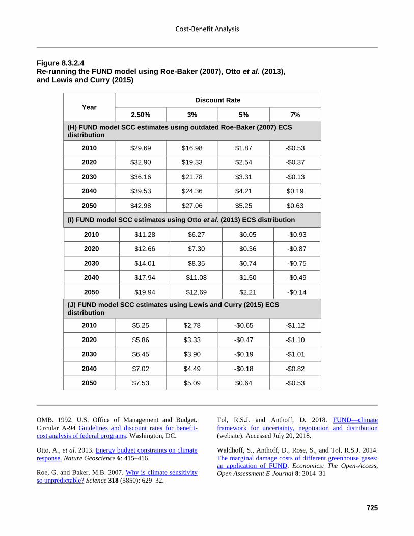
Cost-Benefit Analysis

725

Figure 8.3.2.4 Re-running the FUND model using Roe-Baker (2007), Otto et al. (2013), and Lewis and Curry (2015)

Year Discount Rate

2.50% 3% 5% 7%

(H) FUND model SCC estimates using outdated Roe-Baker (2007) ECS distribution

2010 $29.69 $16.98 $1.87 -$0.53

2020 $32.90 $19.33 $2.54 -$0.37

2030 $36.16 $21.78 $3.31 -$0.13

2040 $39.53 $24.36 $4.21 $0.19

2050 $42.98 $27.06 $5.25 $0.63

(I) FUND model SCC estimates using Otto et al. (2013) ECS distribution

2010 $11.28 $6.27 $0.05 -$0.93

2020 $12.66 $7.30 $0.36 -$0.87

2030 $14.01 $8.35 $0.74 -$0.75

2040 $17.94 $11.08 $1.50 -$0.49

2050 $19.94 $12.69 $2.21 -$0.14

(J) FUND model SCC estimates using Lewis and Curry (2015) ECS distribution

2010 $5.25 $2.78 -$0.65 -$1.12

2020 $5.86 $3.33 -$0.47 -$1.10

2030 $6.45 $3.90 -$0.19 -$1.01

2040 $7.02 $4.49 -$0.18 -$0.82

2050 $7.53 $5.09 $0.64 -$0.53

OMB. 1992. U.S. Office of Management and Budget.

Circular A-94 Guidelines and discount rates for benefit-

cost analysis of federal programs. Washington, DC.

Otto, A., et al. 2013. Energy budget constraints on climate

response. Nature Geoscience 6: 415–416.

Roe, G. and Baker, M.B. 2007. Why is climate sensitivity

so unpredictable? Science 318 (5850): 629–32.

Tol, R.S.J. and Anthoff, D. 2018. FUND—climate

framework for uncertainty, negotiation and distribution

(website). Accessed July 20, 2018.

Waldhoff, S., Anthoff, D., Rose, S., and Tol, R.S.J. 2014.

The marginal damage costs of different greenhouse gases:

an application of FUND. Economics: The Open-Access,

Open Assessment E-Journal 8: 2014–31

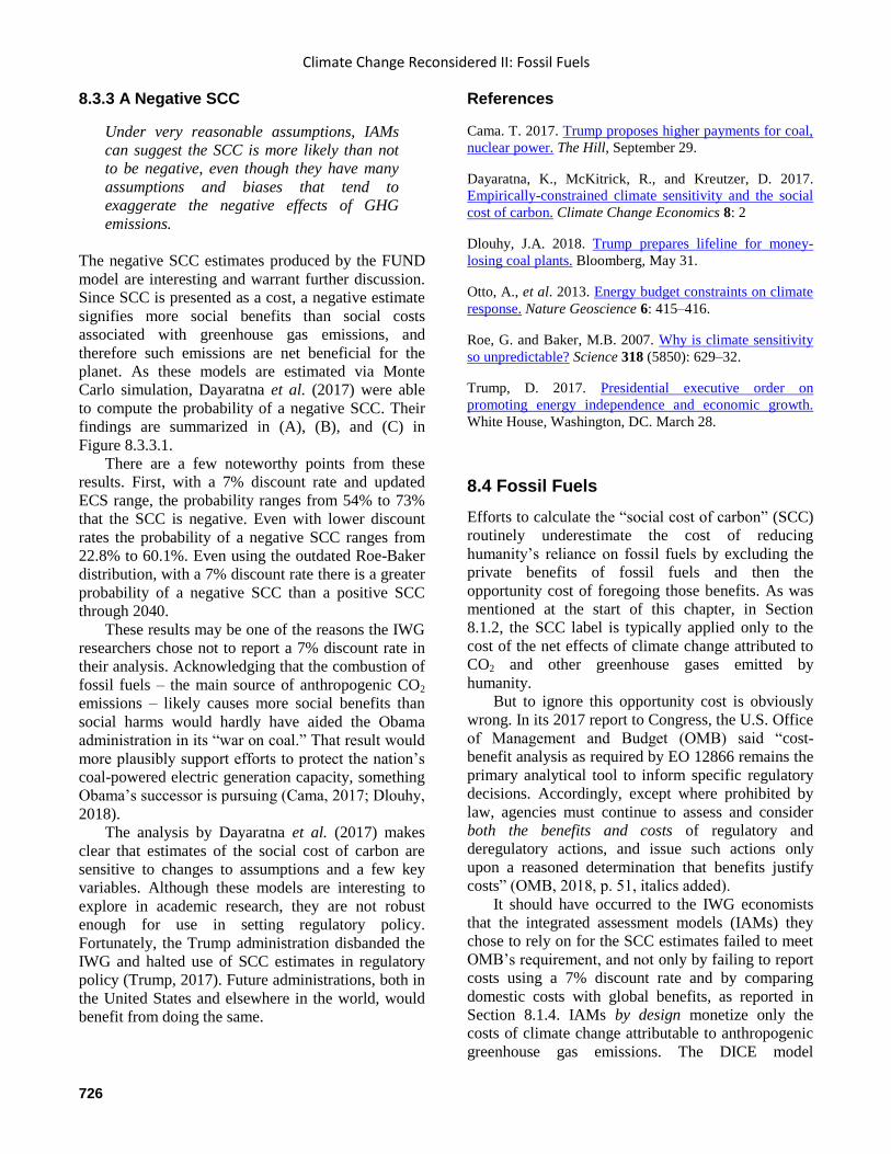
Climate Change Reconsidered II: Fossil Fuels

726

8.3.3 A Negative SCC

Under very reasonable assumptions, IAMs

can suggest the SCC is more likely than not

to be negative, even though they have many

assumptions and biases that tend to

exaggerate the negative effects of GHG

emissions.

The negative SCC estimates produced by the FUND

model are interesting and warrant further discussion.

Since SCC is presented as a cost, a negative estimate

signifies more social benefits than social costs

associated with greenhouse gas emissions, and

therefore such emissions are net beneficial for the

planet. As these models are estimated via Monte

Carlo simulation, Dayaratna et al. (2017) were able

to compute the probability of a negative SCC. Their

findings are summarized in (A), (B), and (C) in

Figure 8.3.3.1.

There are a few noteworthy points from these

results. First, with a 7% discount rate and updated

ECS range, the probability ranges from 54% to 73%

that the SCC is negative. Even with lower discount

rates the probability of a negative SCC ranges from

22.8% to 60.1%. Even using the outdated Roe-Baker

distribution, with a 7% discount rate there is a greater

probability of a negative SCC than a positive SCC

through 2040.

These results may be one of the reasons the IWG

researchers chose not to report a 7% discount rate in

their analysis. Acknowledging that the combustion of

fossil fuels – the main source of anthropogenic CO2

emissions – likely causes more social benefits than

social harms would hardly have aided the Obama

administration in its “war on coal.” That result would

more plausibly support efforts to protect the nation’s

coal-powered electric generation capacity, something

Obama’s successor is pursuing (Cama, 2017; Dlouhy,

2018).

The analysis by Dayaratna et al. (2017) makes

clear that estimates of the social cost of carbon are

sensitive to changes to assumptions and a few key

variables. Although these models are interesting to

explore in academic research, they are not robust

enough for use in setting regulatory policy.

Fortunately, the Trump administration disbanded the

IWG and halted use of SCC estimates in regulatory

policy (Trump, 2017). Future administrations, both in

the United States and elsewhere in the world, would

benefit from doing the same.

References

Cama. T. 2017. Trump proposes higher payments for coal,

nuclear power. The Hill, September 29.

Dayaratna, K., McKitrick, R., and Kreutzer, D. 2017.

Empirically-constrained climate sensitivity and the social

cost of carbon. Climate Change Economics 8: 2

Dlouhy, J.A. 2018. Trump prepares lifeline for money-

losing coal plants. Bloomberg, May 31.

Otto, A., et al. 2013. Energy budget constraints on climate

response. Nature Geoscience 6: 415–416.

Roe, G. and Baker, M.B. 2007. Why is climate sensitivity

so unpredictable? Science 318 (5850): 629–32.

Trump, D. 2017. Presidential executive order on

promoting energy independence and economic growth.

White House, Washington, DC. March 28.

8.4 Fossil Fuels

Efforts to calculate the “social cost of carbon” (SCC)

routinely underestimate the cost of reducing

humanity’s reliance on fossil fuels by excluding the

private benefits of fossil fuels and then the

opportunity cost of foregoing those benefits. As was

mentioned at the start of this chapter, in Section

8.1.2, the SCC label is typically applied only to the

cost of the net effects of climate change attributed to

CO2 and other greenhouse gases emitted by

humanity.

But to ignore this opportunity cost is obviously

wrong. In its 2017 report to Congress, the U.S. Office

of Management and Budget (OMB) said “cost-

benefit analysis as required by EO 12866 remains the

primary analytical tool to inform specific regulatory

decisions. Accordingly, except where prohibited by

law, agencies must continue to assess and consider

both the benefits and costs of regulatory and

deregulatory actions, and issue such actions only

upon a reasoned determination that benefits justify

costs” (OMB, 2018, p. 51, italics added).

It should have occurred to the IWG economists

that the integrated assessment models (IAMs) they

chose to rely on for the SCC estimates failed to meet

OMB’s requirement, and not only by failing to report

costs using a 7% discount rate and by comparing

domestic costs with global benefits, as reported in

Section 8.1.4. IAMs by design monetize only the

costs of climate change attributable to anthropogenic

greenhouse gas emissions. The DICE model

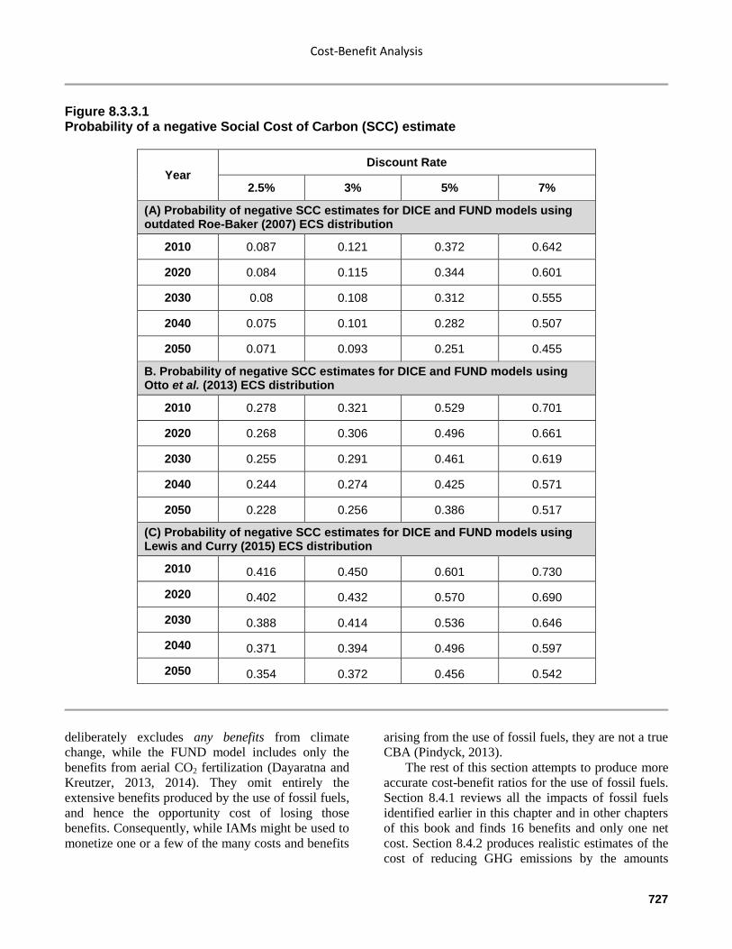
Cost-Benefit Analysis

727

Figure 8.3.3.1 Probability of a negative Social Cost of Carbon (SCC) estimate

Year Discount Rate

2.5% 3% 5% 7%

(A) Probability of negative SCC estimates for DICE and FUND models using outdated Roe-Baker (2007) ECS distribution

2010 0.087 0.121 0.372 0.642

2020 0.084 0.115 0.344 0.601

2030 0.08 0.108 0.312 0.555

2040 0.075 0.101 0.282 0.507

2050 0.071 0.093 0.251 0.455

B. Probability of negative SCC estimates for DICE and FUND models using Otto et al. (2013) ECS distribution

2010 0.278 0.321 0.529 0.701

2020 0.268 0.306 0.496 0.661

2030 0.255 0.291 0.461 0.619

2040 0.244 0.274 0.425 0.571

2050 0.228 0.256 0.386 0.517

(C) Probability of negative SCC estimates for DICE and FUND models using Lewis and Curry (2015) ECS distribution

2010 0.416 0.450 0.601 0.730

2020 0.402 0.432 0.570 0.690

2030 0.388 0.414 0.536 0.646

2040 0.371 0.394 0.496 0.597

2050 0.354 0.372 0.456 0.542

deliberately excludes any benefits from climate

change, while the FUND model includes only the

benefits from aerial CO2 fertilization (Dayaratna and

Kreutzer, 2013, 2014). They omit entirely the

extensive benefits produced by the use of fossil fuels,

and hence the opportunity cost of losing those

benefits. Consequently, while IAMs might be used to

monetize one or a few of the many costs and benefits

arising from the use of fossil fuels, they are not a true

CBA (Pindyck, 2013).

The rest of this section attempts to produce more

accurate cost-benefit ratios for the use of fossil fuels.

Section 8.4.1 reviews all the impacts of fossil fuels

identified earlier in this chapter and in other chapters

of this book and finds 16 benefits and only one net

cost. Section 8.4.2 produces realistic estimates of the

cost of reducing GHG emissions by the amounts

Climate Change Reconsidered II: Fossil Fuels

728

recommended by the IPCC and according to a goal

set by the European Union. Section 8.4.3 produces

new cost-benefit ratios using the findings from the

IPCC, the Interagency Working Group, and Bezdek

(2014, 2015). The authors find the cost of reducing

humanity’s reliance on fossil exceeds the benefits by

ratios as low as 6.8:1 to as high as 160:1.

References

Bezdek, R.H. 2014. The Social Costs of Carbon? No, the

Social Benefits of Carbon. Oakton, VA: Management

Information Services, Inc.

Bezdek, R.H. 2015. Economic and social implications of

potential UN Paris 2015 global GHG reduction mandates.

Oakton, VA: Management Information Services, Inc.

Dayaratna, K. and Kreutzer, D. 2013. Loaded DICE: an

EPA model not ready for the big game. Backgrounder No.

2860. The Heritage Foundation. November 21.

Dayaratna, K. and Kreutzer, D. 2014. Unfounded FUND:

yet another EPA model not ready for the big game.

Backgrounder No. 2897. The Heritage Foundation. April

29.

OMB, 2018. U.S. Office of Management and Budget.

Draft report to Congress on the benefits and costs of

federal regulations and agency compliance with the

Unfunded Mandates Reform Act. February.

Pindyck, R.S. 2013. Climate change policy: what do the

models tell us? Journal of Economic Literature 51 (3):

860–72.

Section 8.4.1 Impacts of Fossil Fuels

Sixteen of 25 possible impacts of fossil fuels

on human well-being are net benefits, only

one is a net cost, and the rest are either

unknown or likely to have no net impact.

The authors of the Working Group II contribution to

the IPCC’s Fifth Assessment Report (AR5) reported

hundreds of studies allegedly documenting the

impacts of climate change on humanity, but they did

not attempt to aggregate those impacts, observing

that differences in methodology, geographical areas,

time periods, and outputs made such a meta-analysis

impossible. Instead, they opted to summarize the

possible impacts in a table (Assessment Box SPM.2

Table 1 in the Summary for Policymakers (IPCC,

2014a, pp. 21–25).

The authors of the current volume follow the

IPCC’s lead by producing the table shown in Figure

8.4.1.1 summarizing the findings of previous chapters

regarding the impacts of fossil fuels on human well-

being. Possible impacts appear in alphabetical order,

their net impact (benefit, cost, no net impact, or

unknown) appear in the second column, brief

observations on the impacts appear in the third

column, and chapters and sections of chapters in

which the topics are addressed appear in the fourth

column of the table.

Figure 8.4.1.1 Impact of fossil fuels on human well-being

Impact Benefit or Cost

Observations Chapter References

Acid rain No net impact Once feared to be a major environmental threat, the deposition of sulfuric and nitric acid due to smokestack emissions, so-called “acid rain,” was later found not to be a threat to forest health and to affect only a few bodies of water, where remediation with lime is an inexpensive solution. The fertilizing effect of nitrogen deposition more than offsets its harms to vegetation. Dramatic reductions in SO2 and NO2 emissions since the 1980s mean “acid rain” has no net impact on human well-being today.

5.1, 6.1

Agriculture Benefit Fossil fuels have contributed to the enormous improvement in crop yields by making artificial fertilizers, mechanization, and modern food processing techniques possible. Higher atmospheric CO2 levels are causing plants to grow better and require less water. Numerous

3.4, 4.1, 5.2, 5.3, 7.2, 8.2

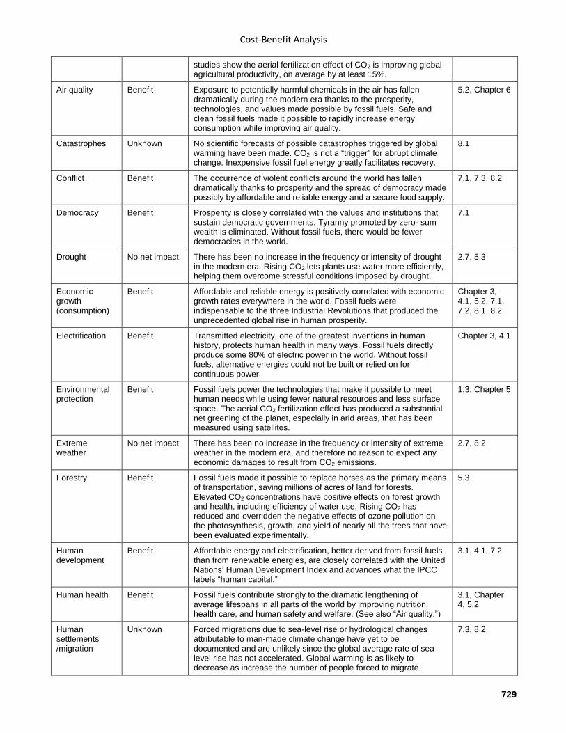
Cost-Benefit Analysis

729

studies show the aerial fertilization effect of CO2 is improving global agricultural productivity, on average by at least 15%.

Air quality Benefit Exposure to potentially harmful chemicals in the air has fallen dramatically during the modern era thanks to the prosperity, technologies, and values made possible by fossil fuels. Safe and clean fossil fuels made it possible to rapidly increase energy consumption while improving air quality.

5.2, Chapter 6

Catastrophes Unknown No scientific forecasts of possible catastrophes triggered by global warming have been made. CO2 is not a “trigger” for abrupt climate change. Inexpensive fossil fuel energy greatly facilitates recovery.

8.1

Conflict Benefit The occurrence of violent conflicts around the world has fallen dramatically thanks to prosperity and the spread of democracy made possibly by affordable and reliable energy and a secure food supply.

7.1, 7.3, 8.2

Democracy Benefit Prosperity is closely correlated with the values and institutions that sustain democratic governments. Tyranny promoted by zero- sum wealth is eliminated. Without fossil fuels, there would be fewer democracies in the world.

7.1

Drought No net impact There has been no increase in the frequency or intensity of drought in the modern era. Rising CO2 lets plants use water more efficiently, helping them overcome stressful conditions imposed by drought.

2.7, 5.3

Economic growth (consumption)

Benefit Affordable and reliable energy is positively correlated with economic growth rates everywhere in the world. Fossil fuels were indispensable to the three Industrial Revolutions that produced the unprecedented global rise in human prosperity.

Chapter 3, 4.1, 5.2, 7.1, 7.2, 8.1, 8.2

Electrification Benefit Transmitted electricity, one of the greatest inventions in human history, protects human health in many ways. Fossil fuels directly produce some 80% of electric power in the world. Without fossil fuels, alternative energies could not be built or relied on for continuous power.

Chapter 3, 4.1

Environmental protection

Benefit Fossil fuels power the technologies that make it possible to meet human needs while using fewer natural resources and less surface space. The aerial CO2 fertilization effect has produced a substantial net greening of the planet, especially in arid areas, that has been measured using satellites.

1.3, Chapter 5

Extreme weather

No net impact There has been no increase in the frequency or intensity of extreme weather in the modern era, and therefore no reason to expect any economic damages to result from CO2 emissions.

2.7, 8.2

Forestry Benefit Fossil fuels made it possible to replace horses as the primary means of transportation, saving millions of acres of land for forests. Elevated CO2 concentrations have positive effects on forest growth and health, including efficiency of water use. Rising CO2 has reduced and overridden the negative effects of ozone pollution on the photosynthesis, growth, and yield of nearly all the trees that have been evaluated experimentally.

5.3

Human development

Benefit Affordable energy and electrification, better derived from fossil fuels than from renewable energies, are closely correlated with the United Nations’ Human Development Index and advances what the IPCC labels “human capital.”

3.1, 4.1, 7.2

Human health Benefit Fossil fuels contribute strongly to the dramatic lengthening of average lifespans in all parts of the world by improving nutrition, health care, and human safety and welfare. (See also “Air quality.”)

3.1, Chapter 4, 5.2

Human settlements /migration

Unknown Forced migrations due to sea-level rise or hydrological changes attributable to man-made climate change have yet to be documented and are unlikely since the global average rate of sea-level rise has not accelerated. Global warming is as likely to decrease as increase the number of people forced to migrate.

7.3, 8.2

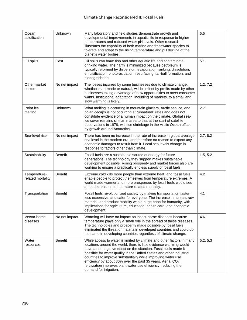
Climate Change Reconsidered II: Fossil Fuels

730

Ocean acidification

Unknown Many laboratory and field studies demonstrate growth and developmental improvements in aquatic life in response to higher temperatures and reduced water pH levels. Other research illustrates the capability of both marine and freshwater species to tolerate and adapt to the rising temperature and pH decline of the planet’s water bodies.

5.5

Oil spills Cost Oil spills can harm fish and other aquatic life and contaminate drinking water. The harm is minimized because petroleum is typically reformed by dispersion, evaporation, sinking, dissolution, emulsification, photo-oxidation, resurfacing, tar-ball formation, and biodegradation.

5.1

Other market sectors

No net impact The losses incurred by some businesses due to climate change, whether man-made or natural, will be offset by profits made by other businesses taking advantage of new opportunities to meet consumer wants. Institutional adaptation, including of markets, to a small and slow warming is likely.

1.2, 7.2

Polar ice melting

Unknown What melting is occurring in mountain glaciers, Arctic sea ice, and polar icecaps is not occurring at “unnatural” rates and does not constitute evidence of a human impact on the climate. Global sea-ice cover remains similar in area to that at the start of satellite observations in 1979, with ice shrinkage in the Arctic Ocean offset by growth around Antarctica.

2.7

Sea-level rise No net impact There has been no increase in the rate of increase in global average sea level in the modern era, and therefore no reason to expect any economic damages to result from it. Local sea levels change in response to factors other than climate.

2.7, 8.2

Sustainability Benefit Fossil fuels are a sustainable source of energy for future generations. The technology they support makes sustainable development possible. Rising prosperity and market forces also are working to ensure a practically endless supply of fossil fuels.

1.5, 5.2

Temperature-related mortality

Benefit Extreme cold kills more people than extreme heat, and fossil fuels enable people to protect themselves from temperature extremes. A world made warmer and more prosperous by fossil fuels would see a net decrease in temperature-related mortality.

4.2

Transportation Benefit Fossil fuels revolutionized society by making transportation faster, less expensive, and safer for everyone. The increase in human, raw material, and product mobility was a huge boon for humanity, with implications for agriculture, education, health care, and economic development.

4.1

Vector-borne diseases

No net impact Warming will have no impact on insect-borne diseases because temperature plays only a small role in the spread of these diseases. The technologies and prosperity made possible by fossil fuels eliminated the threat of malaria in developed countries and could do the same in developing countries regardless of climate change.

4.6

Water resources

Benefit While access to water is limited by climate and other factors in many locations around the world, there is little evidence warming would have a net negative effect on the situation. Fossil fuels made it possible for water quality in the United States and other industrial countries to improve substantially while improving water use efficiency by about 30% over the past 35 years. Aerial CO2 fertilization improves plant water use efficiency, reducing the demand for irrigation.

5.2, 5.3

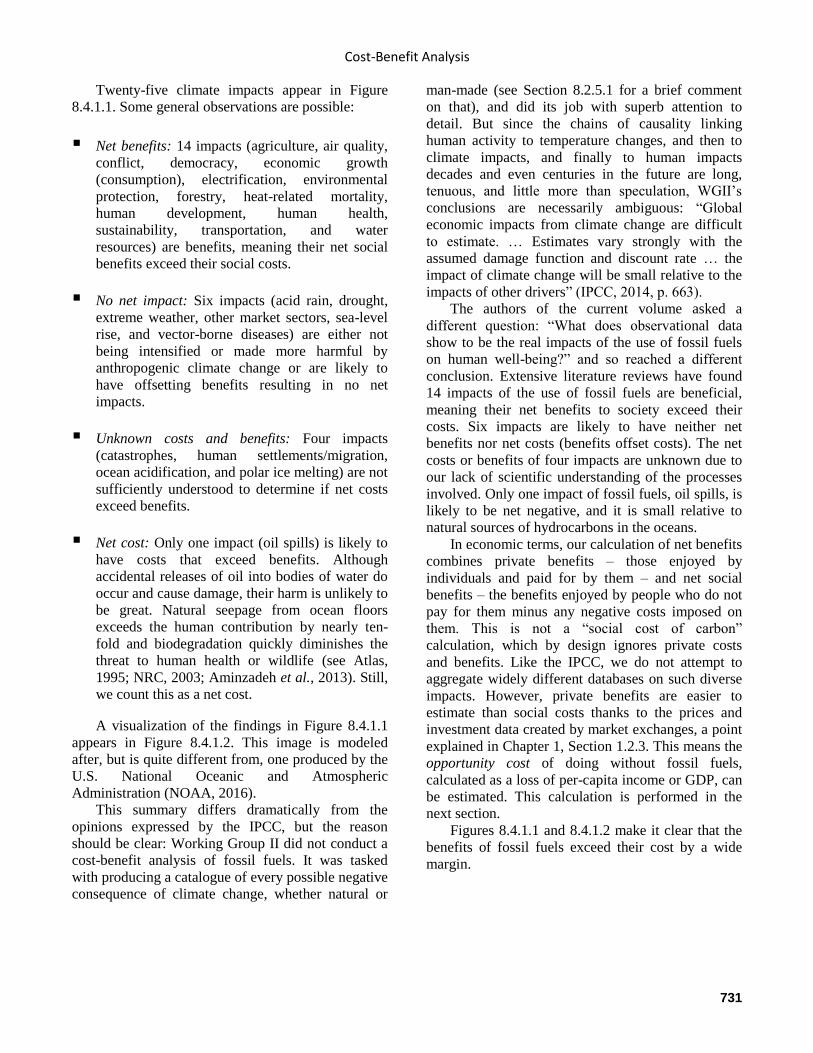
Cost-Benefit Analysis

731

Twenty-five climate impacts appear in Figure

8.4.1.1. Some general observations are possible:

Net benefits: 14 impacts (agriculture, air quality,

conflict, democracy, economic growth

(consumption), electrification, environmental

protection, forestry, heat-related mortality,

human development, human health,

sustainability, transportation, and water

resources) are benefits, meaning their net social

benefits exceed their social costs.

No net impact: Six impacts (acid rain, drought,

extreme weather, other market sectors, sea-level

rise, and vector-borne diseases) are either not

being intensified or made more harmful by

anthropogenic climate change or are likely to

have offsetting benefits resulting in no net

impacts.

Unknown costs and benefits: Four impacts

(catastrophes, human settlements/migration,

ocean acidification, and polar ice melting) are not

sufficiently understood to determine if net costs

exceed benefits.

Net cost: Only one impact (oil spills) is likely to

have costs that exceed benefits. Although

accidental releases of oil into bodies of water do

occur and cause damage, their harm is unlikely to

be great. Natural seepage from ocean floors

exceeds the human contribution by nearly ten-

fold and biodegradation quickly diminishes the

threat to human health or wildlife (see Atlas,

1995; NRC, 2003; Aminzadeh et al., 2013). Still,

we count this as a net cost.

A visualization of the findings in Figure 8.4.1.1

appears in Figure 8.4.1.2. This image is modeled

after, but is quite different from, one produced by the

U.S. National Oceanic and Atmospheric

Administration (NOAA, 2016).

This summary differs dramatically from the

opinions expressed by the IPCC, but the reason

should be clear: Working Group II did not conduct a

cost-benefit analysis of fossil fuels. It was tasked

with producing a catalogue of every possible negative

consequence of climate change, whether natural or

man-made (see Section 8.2.5.1 for a brief comment

on that), and did its job with superb attention to

detail. But since the chains of causality linking

human activity to temperature changes, and then to

climate impacts, and finally to human impacts

decades and even centuries in the future are long,

tenuous, and little more than speculation, WGII’s

conclusions are necessarily ambiguous: “Global

economic impacts from climate change are difficult

to estimate. … Estimates vary strongly with the

assumed damage function and discount rate … the

impact of climate change will be small relative to the

impacts of other drivers” (IPCC, 2014, p. 663).

The authors of the current volume asked a

different question: “What does observational data

show to be the real impacts of the use of fossil fuels

on human well-being?” and so reached a different

conclusion. Extensive literature reviews have found

14 impacts of the use of fossil fuels are beneficial,

meaning their net benefits to society exceed their

costs. Six impacts are likely to have neither net

benefits nor net costs (benefits offset costs). The net

costs or benefits of four impacts are unknown due to

our lack of scientific understanding of the processes

involved. Only one impact of fossil fuels, oil spills, is

likely to be net negative, and it is small relative to

natural sources of hydrocarbons in the oceans.

In economic terms, our calculation of net benefits

combines private benefits – those enjoyed by

individuals and paid for by them – and net social

benefits – the benefits enjoyed by people who do not

pay for them minus any negative costs imposed on

them. This is not a “social cost of carbon”

calculation, which by design ignores private costs

and benefits. Like the IPCC, we do not attempt to

aggregate widely different databases on such diverse

impacts. However, private benefits are easier to

estimate than social costs thanks to the prices and

investment data created by market exchanges, a point

explained in Chapter 1, Section 1.2.3. This means the

opportunity cost of doing without fossil fuels,

calculated as a loss of per-capita income or GDP, can

be estimated. This calculation is performed in the

next section.

Figures 8.4.1.1 and 8.4.1.2 make it clear that the

benefits of fossil fuels exceed their cost by a wide

margin.

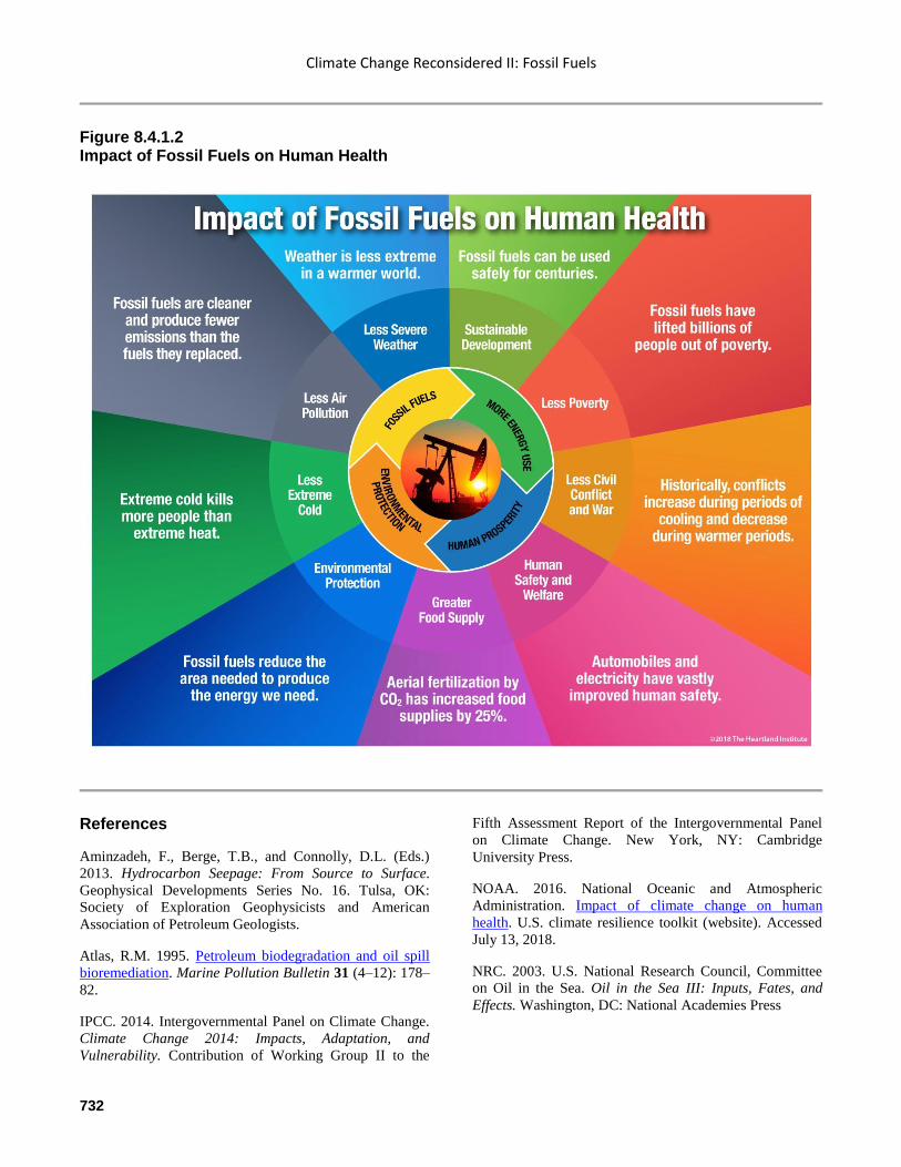
Climate Change Reconsidered II: Fossil Fuels

732

Figure 8.4.1.2 Impact of Fossil Fuels on Human Health

References

Aminzadeh, F., Berge, T.B., and Connolly, D.L. (Eds.)

2013. Hydrocarbon Seepage: From Source to Surface.

Geophysical Developments Series No. 16. Tulsa, OK:

Society of Exploration Geophysicists and American

Association of Petroleum Geologists.

Atlas, R.M. 1995. Petroleum biodegradation and oil spill

bioremediation. Marine Pollution Bulletin 31 (4–12): 178–

82.

IPCC. 2014. Intergovernmental Panel on Climate Change.

Climate Change 2014: Impacts, Adaptation, and

Vulnerability. Contribution of Working Group II to the

Fifth Assessment Report of the Intergovernmental Panel

on Climate Change. New York, NY: Cambridge

University Press.

NOAA. 2016. National Oceanic and Atmospheric

Administration. Impact of climate change on human

health. U.S. climate resilience toolkit (website). Accessed

July 13, 2018.

NRC. 2003. U.S. National Research Council, Committee

on Oil in the Sea. Oil in the Sea III: Inputs, Fates, and

Effects. Washington, DC: National Academies Press

Cost-Benefit Analysis

733

8.4.2 Cost of Mitigation

Wind and solar cannot generate enough

dispatchable energy (available 24/7) to

replace fossil fuels, so energy consumption

must fall in order for emissions to fall.

According to the Working Group III contribution to

the IPCC’s Fifth Assessment Report, keeping average

global surface temperature change to less than 2°C

above its pre-industrial level by 2100 requires

limiting atmospheric concentrations of CO2 in 2100

to “about 450 ppm CO2eq (high confidence),” which

would require “substantial cuts in anthropogenic

GHG emissions by mid-century through large scale

changes in energy systems and potentially land use

(high confidence). Scenarios reaching these

concentrations by 2100 are characterized by lower

global GHG emissions in 2050 than in 2010, 40% to

70% lower globally, and emissions levels near zero

GtCO2eq or below in 2100” (IPCC, 2014b, pp. 10,

12). Emissions can supposedly fall to below zero

through the use of “carbon dioxide removal

technologies” (Ibid.).

Also according to Working Group III, the cost of

reducing emissions to meet these goals in the IPCC’s

best-case scenario – where all countries immediately

begin mitigation efforts, adopt a single global carbon

tax, and impose no regulations favoring some

technologies over others – expressed as a percentage

of baseline global gross domestic product (GDP)

without climate policies, would be 1% to 4%

(median: 1.7%) in 2030, 2% to 6% (median: 3.4%) in

2050, and 3% to 11% (median: 4.8%) in 2100

relative to consumption in baseline scenarios (IPCC,

2014b, pp. 15–16, text and Table SPM.2).

The following sections explain why IPCC’s

estimate of the cost of a forced transition away from

fossil fuels to “near zero … or below in 2100” is too

low for two reasons. First, replacing a world energy

system currently dependent on fossil fuels to provide

more than 80% of primary energy with one relying

mostly or entirely on alternative energies would cost

far greater sums and take decades to implement.

Second, wind and solar face physical limits that

prevent them from generating enough dispatchable

energy (available 24/7) to replace fossil fuels, so

energy consumption must fall in order for emissions

to fall. Energy demand is forecast to grow

significantly in the twenty-first century, and the

opportunity cost of reversing that trend – of reducing

rather than increasing per-capita energy consumption

– is enormous. Section 8.4.2.1 addresses the first

concern, and Section 8.4.2.2 addresses the second.

8.4.2.1 High Cost of Reducing Emissions

Transitioning from a world energy system

dependent on fossil fuels to one relying on

alternative energies would cost trillions of

dollars and take decades to implement.

Chapter 3, Section 3.5, documented at great length

the inherent limitations on alternative energy sources

and the history of past transitions to new energy

sources suggesting the cost of forcing a transition

from fossil fuels would be very costly (Smil, 2010;

Morriss et al., 2011; Clack et al., 2017). The sheer

size of the global energy market makes replacing it

massively expensive and time consuming. Smil

(2010) notes the global oil industry “handles about 30

billion barrels annually or 4 billion tons” and

operates about 3,000 large tankers and more than

300,000 miles of pipelines. “Even if an immediate

alternative were available, writing off this colossal

infrastructure that took more than a century to build

would amount to discarding an investment worth well

over $5 trillion – and it is quite obvious that its

energy output could not be replaced by any

alternative in a decade or two” (p. 140). Later, Smil

(2010, p. 148) writes the cost of a transition “would

be easily equal to the total value of U.S. gross

domestic product (GDP), or close to a quarter of the

global economic product.”

Wind and solar power face cost, scale, and

intermittency problems that make extremely

expensive any efforts to increase their share of total

energy production to more than 10% or 15% of total

production. In particular, their low power density

means scaling them up to replace fossil fuels would

require alarming amounts of surface space, crowding

out agriculture and wildlife habitat with harmful

effects on food production and the natural

environment. See Chapter 3, Section 3.2, and Chapter

5, Section 5.2, for discussions of these problems and

many references there (e.g., Rasmussen, 2010;

Hansen, 2011; Kelly, 2014; Bryce, 2014; Smil, 2016;

Stacy and Taylor, 2016; Driessen, 2017).

Advocates of rapid decarbonization

underestimate the negative consequences of the

intermittency of solar and wind power. In a critique

of Jacobson et al. (2015) and an earlier paper also by

Jacobson and a coauthor (Jacobson and Delucchi,

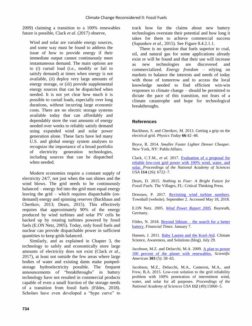
Climate Change Reconsidered II: Fossil Fuels

734

2009) claiming a transition to a 100% renewables

future is possible, Clack et al. (2017) observe,

Wind and solar are variable energy sources,

and some way must be found to address the

issue of how to provide energy if their

immediate output cannot continuously meet

instantaneous demand. The main options are

to (i) curtail load (i.e., modify or fail to

satisfy demand) at times when energy is not

available, (ii) deploy very large amounts of

energy storage, or (iii) provide supplemental

energy sources that can be dispatched when

needed. It is not yet clear how much it is

possible to curtail loads, especially over long

durations, without incurring large economic

costs. There are no electric storage systems

available today that can affordably and

dependably store the vast amounts of energy

needed over weeks to reliably satisfy demand

using expanded wind and solar power

generation alone. These facts have led many

U.S. and global energy system analyses to

recognize the importance of a broad portfolio

of electricity generation technologies,

including sources that can be dispatched

when needed.

Modern economies require a constant supply of

electricity 24/7, not just when the sun shines and the

wind blows. The grid needs to be continuously

balanced – energy fed into the grid must equal energy

leaving the grid – which requires dispatchable (on-

demand) energy and spinning reserves (Backhaus and

Chertkov, 2013; Dears, 2015). This effectively

requires that approximately 90% of the energy

produced by wind turbines and solar PV cells be

backed up by rotating turbines powered by fossil

fuels (E.ON Netz, 2005). Today, only fossil fuels and

nuclear can provide dispatchable power in sufficient

quantities to keep grids balanced.

Similarly, and as explained in Chapter 3, the

technology to safely and economically store large

amounts of electricity does not exist (Clack et al.,

2017), at least not outside the few areas where large

bodies of water and existing dams make pumped-

storage hydroelectricity possible. The frequent

announcements of “breakthroughs” in battery

technology have not resulted in commercial products

capable of even a small fraction of the storage needs

of a transition from fossil fuels (Fildes, 2018).

Scholars have even developed a “hype curve” to

track how far the claims about new battery

technologies overstate their potential and how long it

takes for them to achieve commercial success

(Sapunkov et al., 2015). See Figure 8.4.2.1.1.

There is no question that fuels superior to coal,

oil, and natural gas for some applications already

exist or will be found and that their use will increase

as new technologies are discovered and

commercialized. Energy freedom – relying on

markets to balance the interests and needs of today

with those of tomorrow and to access the local

knowledge needed to find efficient win-win

responses to climate change – should be permitted to

dictate the pace of this transition, not fears of a

climate catastrophe and hope for technological

breakthroughs.

References

Backhaus, S. and Chertkov, M. 2013. Getting a grip on the

electrical grid. Physics Today 66:42–48.

Bryce, R. 2014. Smaller Faster Lighter Denser Cheaper.

New York, NY: PublicAffairs.

Clack, C.T.M., et al. 2017. Evaluation of a proposal for

reliable low-cost grid power with 100% wind, water, and

solar. Proceedings of the National Academy of Sciences

USA 114 (26): 6722–7.

Dears, D. 2015. Nothing to Fear: A Bright Future for

Fossil Fuels. The Villages, FL: Critical Thinking Press.

Driessen, P. 2017. Revisiting wind turbine numbers.

Townhall (website). September 2. Accessed May 18, 2018.

E.ON Netz. 2005. Wind Power Report 2005. Bayreuth,

Germany.

Fildes, N. 2018. Beyond lithium – the search for a better

battery. Financial Times. January 7.

Hansen, J. 2011. Baby Lauren and the Kool-Aid. Climate

Science, Awareness, and Solutions (blog). July 29.

Jacobson, M.Z. and Delucchi, M.A. 2009. A plan to power

100 percent of the planet with renewables. Scientific

American 303 (5): 58–65.

Jacobson, M.Z., Delucchi, M.A., Cameron, M.A., and

Frew, B.A. 2015. Low-cost solution to the grid reliability

problem with 100% penetration of intermittent wind,

water, and solar for all purposes. Proceedings of the

National Academy of Sciences USA 112 (49):15060–5.

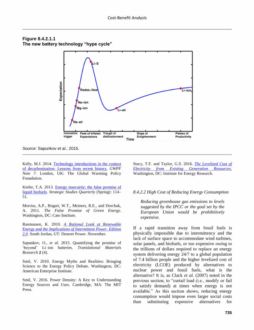
Cost-Benefit Analysis

735

Figure 8.4.2.1.1 The new battery technology “hype cycle”

Source: Sapunkov et al., 2015.

Kelly, M.J. 2014. Technology introductions in the context

of decarbonisation: Lessons from recent history. GWPF

Note 7. London, UK: The Global Warming Policy

Foundation.

Kiefer, T.A. 2013. Energy insecurity: the false promise of

liquid biofuels. Strategic Studies Quarterly (Spring): 114–

51.

Morriss, A.P., Bogart, W.T., Meiners, R.E., and Dorchak,

A. 2011. The False Promise of Green Energy.

Washington, DC: Cato Institute.

Rasmussen, K. 2010. A Rational Look at Renewable

Energy and the Implications of Intermittent Power. Edition

2.0. South Jordan, UT: Deseret Power. November.

Sapunkov, O., et al. 2015. Quantifying the promise of

‘beyond’ Li–ion batteries. Translational Materials

Research 2 (4).

Smil, V. 2010. Energy Myths and Realities: Bringing

Science to the Energy Policy Debate. Washington, DC:

American Enterprise Institute.

Smil, V. 2016. Power Density: A Key to Understanding

Energy Sources and Uses. Cambridge, MA: The MIT

Press.

Stacy, T.F. and Taylor, G.S. 2016. The Levelized Cost of

Electricity from Existing Generation Resources.

Washington, DC: Institute for Energy Research.

8.4.2.2 High Cost of Reducing Energy Consumption

Reducing greenhouse gas emissions to levels

suggested by the IPCC or the goal set by the

European Union would be prohibitively

expensive.

If a rapid transition away from fossil fuels is

physically impossible due to intermittency and the

lack of surface space to accommodate wind turbines,

solar panels, and biofuels, or too expensive owing to

the trillions of dollars required to replace an energy

system delivering energy 24/7 to a global population

of 7.4 billion people and the higher levelized cost of

electricity (LCOE) produced by alternatives to

nuclear power and fossil fuels, what is the

alternative? It is, as Clack et al. (2007) noted in the

previous section, to “curtail load (i.e., modify or fail

to satisfy demand) at times when energy is not

available.” As this section shows, reducing energy

consumption would impose even larger social costs

than substituting expensive alternatives for

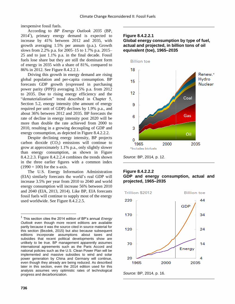
Climate Change Reconsidered II: Fossil Fuels

736

inexpensive fossil fuels.

According to BP Energy Outlook 2035 (BP,

20141), primary energy demand is expected to

increase by 41% between 2012 and 2035, with

growth averaging 1.5% per annum (p.a.). Growth

slows from 2.2% p.a. for 2005–15 to 1.7% p.a. 2015–

25 and to just 1.1% p.a. in the final decade. Fossil

fuels lose share but they are still the dominant form

of energy in 2035 with a share of 81%, compared to

86% in 2012. See Figure 8.4.2.2.1.

Driving this growth in energy demand are rising

global population and per-capita consumption. BP

forecasts GDP growth (expressed in purchasing

power parity (PPP)) averaging 3.5% p.a. from 2012

to 2035. Due to rising energy efficiency and the

“dematerialization” trend described in Chapter 5,

Section 5.2, energy intensity (the amount of energy

required per unit of GDP) declines by 1.9% p.a., and

about 36% between 2012 and 2035. BP forecasts the

rate of decline in energy intensity post 2020 will be

more than double the rate achieved from 2000 to

2010, resulting in a growing decoupling of GDP and

energy consumption, as depicted in Figure 8.4.2.2.2.

Despite declining energy intensity, BP projects

carbon dioxide (CO2) emissions will continue to

grow at approximately 1.1% p.a., only slightly slower

than energy consumption, as shown in Figure

8.4.2.2.3. Figure 8.4.2.2.4 combines the trends shown

in the three earlier figures with a common index

(1990 = 100) for the x-axis.

The U.S. Energy Information Administration

(EIA) similarly forecasts the world’s real GDP will

increase 3.5% per year from 2010 to 2040 and world

energy consumption will increase 56% between 2010

and 2040 (EIA, 2013, 2014). Like BP, EIA forecasts

fossil fuels will continue to supply most of the energy

used worldwide. See Figure 8.4.2.2.5.

1 This section cites the 2014 edition of BP’s annual Energy

Outlook even though more recent editions are available

partly because it was the source cited in source material for this section (Bezdek, 2015) but also because subsequent editions incorporate assumptions about taxes and subsidies that recent political developments show are unlikely to be true. BP management apparently assumes international agreements such as the Paris Accord and national policies such as the U.S. Clean Power Plan will be implemented and massive subsidies to wind and solar power generation by China and Germany will continue, even though they already are being reduced. As described later in this section, even the 2014 edition used for this analysis assumes very optimistic rates of technological progress and decarbonization.

Figure 8.4.2.2.1 Global energy consumption by type of fuel, actual and projected, in billion tons of oil equivalent (toe), 1965–2035

Source: BP, 2014, p. 12.

Figure 8.4.2.2.2 GDP and energy consumption, actual and projected, 1965–2035

Source: BP, 2014, p. 16.

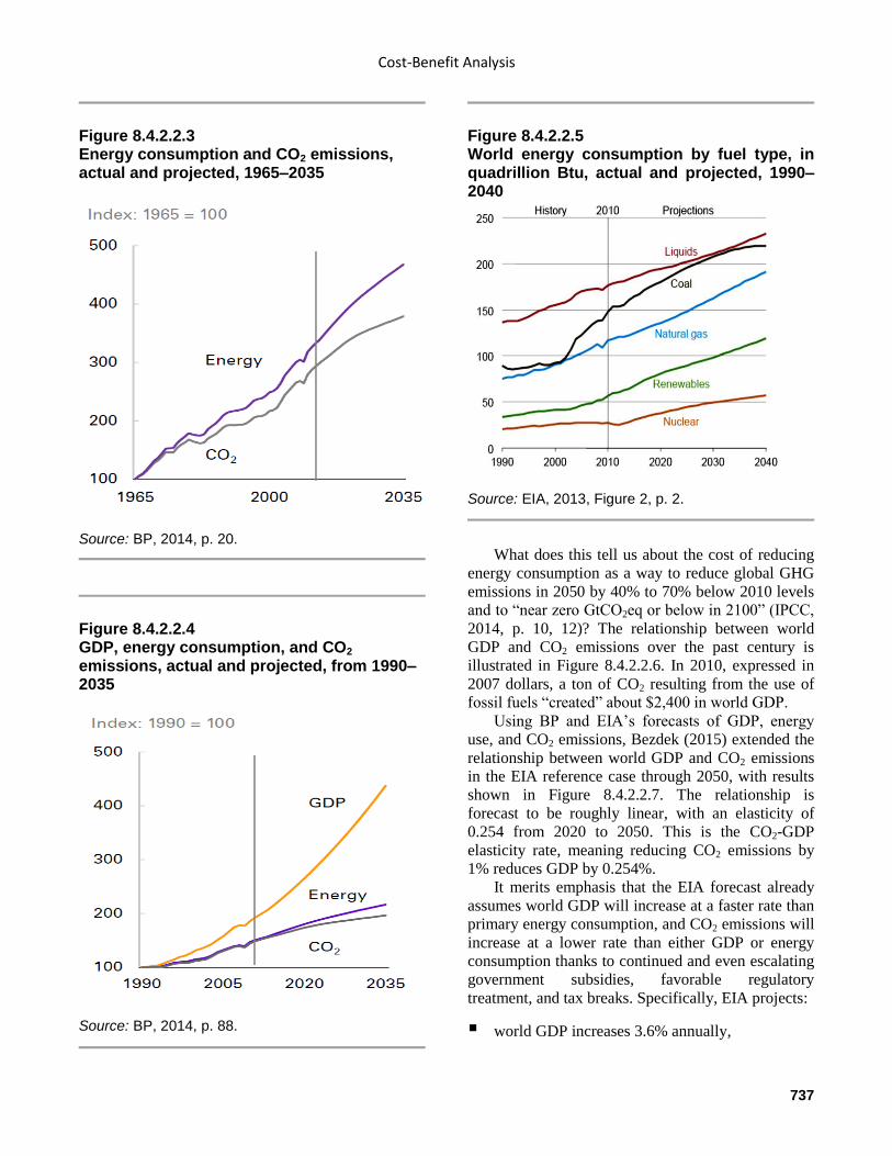
Cost-Benefit Analysis

737

Figure 8.4.2.2.3 Energy consumption and CO2 emissions, actual and projected, 1965–2035

Source: BP, 2014, p. 20.

Figure 8.4.2.2.4 GDP, energy consumption, and CO2 emissions, actual and projected, from 1990–2035

Source: BP, 2014, p. 88.

Figure 8.4.2.2.5 World energy consumption by fuel type, in quadrillion Btu, actual and projected, 1990–2040

Source: EIA, 2013, Figure 2, p. 2.

What does this tell us about the cost of reducing

energy consumption as a way to reduce global GHG

emissions in 2050 by 40% to 70% below 2010 levels

and to “near zero GtCO2eq or below in 2100” (IPCC,

2014, p. 10, 12)? The relationship between world

GDP and CO2 emissions over the past century is

illustrated in Figure 8.4.2.2.6. In 2010, expressed in

2007 dollars, a ton of CO2 resulting from the use of

fossil fuels “created” about $2,400 in world GDP.

Using BP and EIA’s forecasts of GDP, energy

use, and CO2 emissions, Bezdek (2015) extended the

relationship between world GDP and CO2 emissions

in the EIA reference case through 2050, with results

shown in Figure 8.4.2.2.7. The relationship is

forecast to be roughly linear, with an elasticity of

0.254 from 2020 to 2050. This is the CO2-GDP

elasticity rate, meaning reducing CO2 emissions by

1% reduces GDP by 0.254%.

It merits emphasis that the EIA forecast already

assumes world GDP will increase at a faster rate than

primary energy consumption, and CO2 emissions will

increase at a lower rate than either GDP or energy

consumption thanks to continued and even escalating

government subsidies, favorable regulatory

treatment, and tax breaks. Specifically, EIA projects:

world GDP increases 3.6% annually,

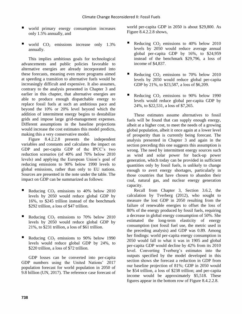
Climate Change Reconsidered II: Fossil Fuels

738

world primary energy consumption increases

only 1.5% annually, and

world CO2 emissions increase only 1.3%

annually.

This implies ambitious goals for technological

advancements and public policies favorable to

alternative energies are already incorporated into

these forecasts, meaning even more programs aimed

at speeding a transition to alternative fuels would be

increasingly difficult and expensive. It also assumes,

contrary to the analysis presented in Chapter 3 and

earlier in this chapter, that alternative energies are

able to produce enough dispatchable energy to

replace fossil fuels at such an ambitious pace and

beyond the 10% or 20% level beyond which the

addition of intermittent energy begins to destabilize

grids and impose large grid-management expenses.

Different assumptions in the baseline projections

would increase the cost estimates this model predicts,

making this a very conservative model.

Figure 8.4.2.2.8 presents the independent

variables and constants and calculates the impact on

GDP and per-capita GDP of the IPCC’s two

reduction scenarios (of 40% and 70% below 2010

levels) and applying the European Union’s goal of

reducing emissions to 90% below 1990 levels to

global emissions, rather than only to EU nations.

Sources are presented in the note under the table. The

impact on GDP can be summarized as follows:

Reducing CO2 emissions to 40% below 2010

levels by 2050 would reduce global GDP by

16%, to $245 trillion instead of the benchmark

$292 trillion, a loss of $47 trillion.

Reducing CO2 emissions to 70% below 2010

levels by 2050 would reduce global GDP by

21%, to $231 trillion, a loss of $61 trillion.

Reducing CO2 emissions to 90% below 1990

levels would reduce global GDP by 24%, to

$220 trillion, a loss of $72 trillion.

GDP losses can be converted into per-capita

GDP numbers using the United Nations’ 2017

population forecast for world population in 2050 of

9.8 billion (UN, 2017). The reference case forecast of

world per-capita GDP in 2050 is about $29,800. As

Figure 8.4.2.2.8 shows,

Reducing CO2 emissions to 40% below 2010

levels by 2050 would reduce average annual

global per-capita GDP by 16%, to $24,959

instead of the benchmark $29,796, a loss of

income of $4,837.

Reducing CO2 emissions to 70% below 2010

levels by 2050 would reduce global per-capita

GDP by 21%, to $23,587, a loss of $6,209.

Reducing CO2 emissions to 90% below 1990

levels would reduce global per-capita GDP by

24%, to $22,531, a loss of $7,265.

These estimates assume alternatives to fossil

fuels will be found that can supply enough energy,

albeit at a higher cost, to meet the needs of a growing

global population, albeit it once again at a lower level

of prosperity than is currently being forecast. The

analysis presented in Chapter 3 and again in the

section preceding this one suggests this assumption is

wrong. The need by intermittent energy sources such

as wind and solar power for back-up power

generation, which today can be provided in sufficient

quantities only by fossil fuels, is unlikely to change

enough to avert energy shortages, particularly in

those countries that have chosen to abandon their

coal, natural gas, and nuclear energy generation

capacity.

Recall from Chapter 3, Section 3.6.2, the

calculation by Tverberg (2012), who sought to

measure the lost GDP in 2050 resulting from the

failure of renewable energies to offset the loss of

80% of the energy produced by fossil fuels, requiring

a decrease in global energy consumption of 50%. She

estimated the long-term elasticity of energy

consumption (not fossil fuel use, the metric used in

the preceding analysis) and GDP was 0.89. Among

her findings: world per-capita energy consumption in

2050 would fall to what it was in 1905 and global

per-capita GDP would decline by 42% from its 2010

level. Converting Tverberg’s estimates into the

outputs specified by the model developed in this

section shows she forecast a reduction in GDP from

our baseline projection of 81%; GDP in 2050 would

be $54 trillion, a loss of $238 trillion; and per-capita

income would be approximately $5,518. These

figures appear in the bottom row of Figure 8.4.2.2.8.

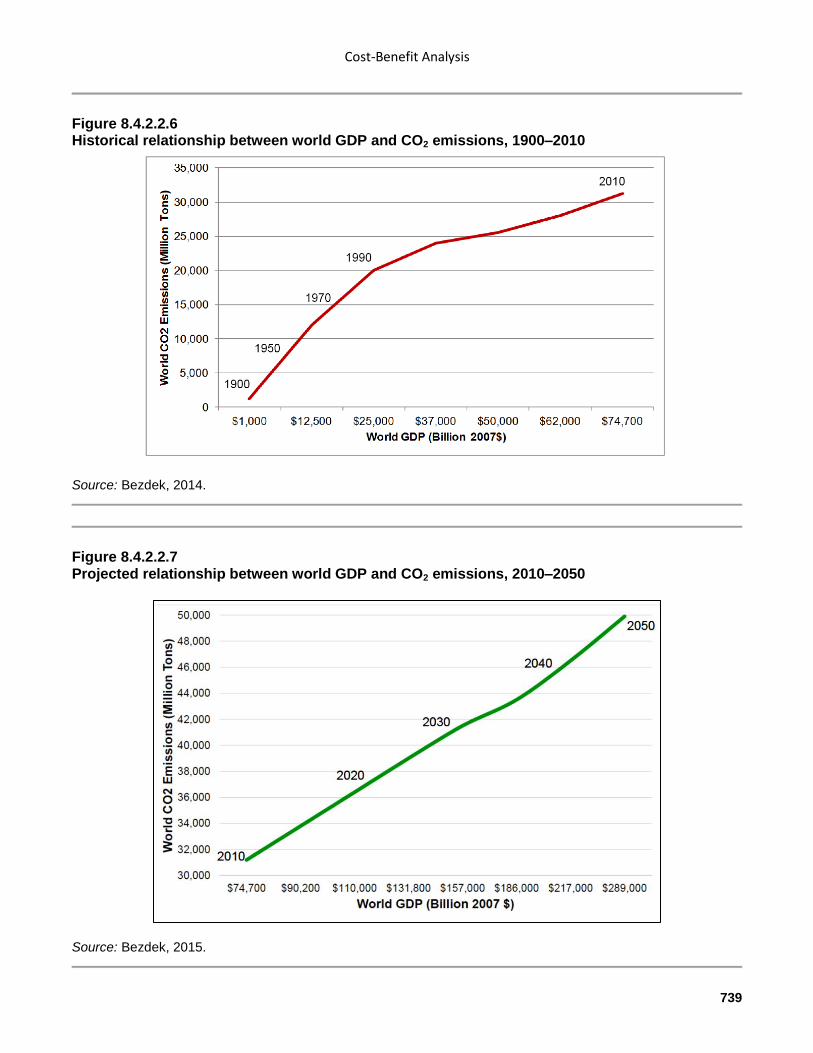
Cost-Benefit Analysis

739

Figure 8.4.2.2.6 Historical relationship between world GDP and CO2 emissions, 1900–2010

Source: Bezdek, 2014.

Figure 8.4.2.2.7 Projected relationship between world GDP and CO2 emissions, 2010–2050

Source: Bezdek, 2015.

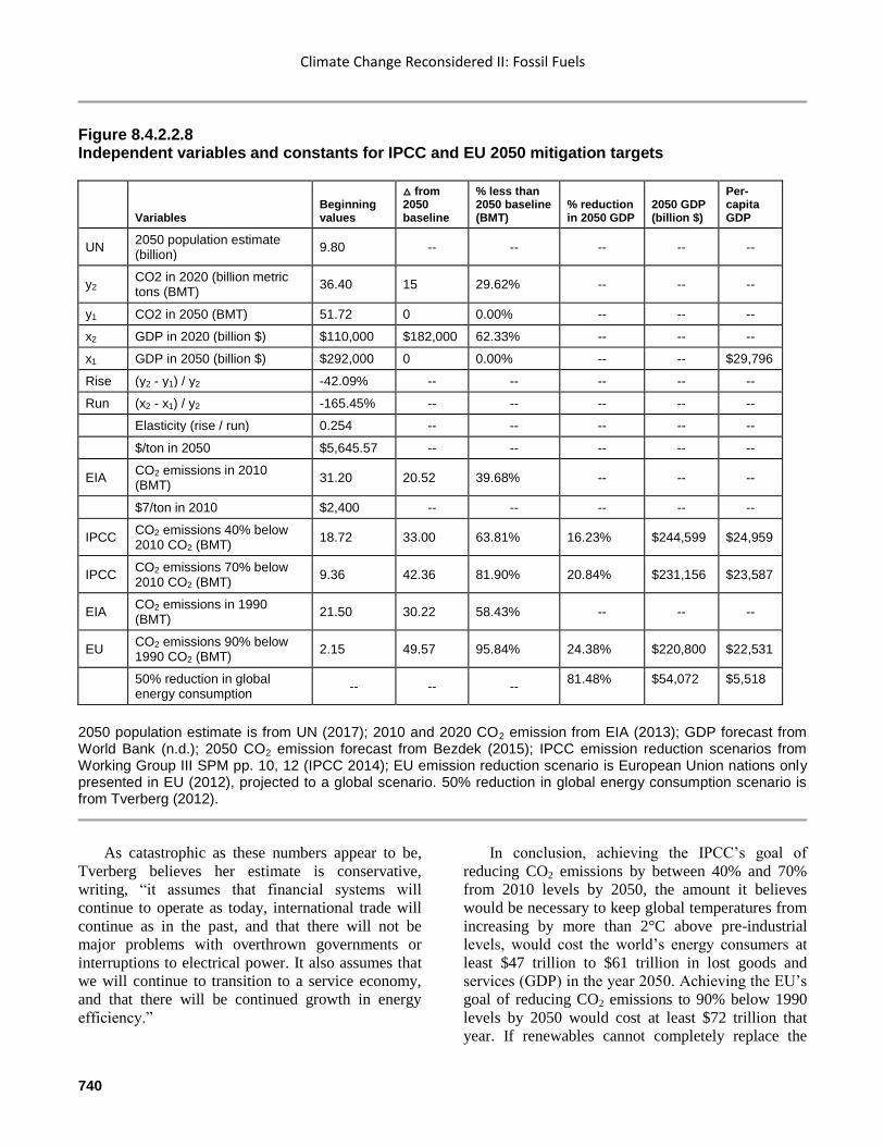
Climate Change Reconsidered II: Fossil Fuels

740

Figure 8.4.2.2.8 Independent variables and constants for IPCC and EU 2050 mitigation targets

Variables Beginning values

△ from 2050 baseline

% less than 2050 baseline (BMT)

% reduction in 2050 GDP

2050 GDP (billion $)

Per-capita GDP

UN 2050 population estimate (billion)

9.80 -- -- -- -- --

y2 CO2 in 2020 (billion metric tons (BMT)

36.40 15 29.62% -- -- --

y1 CO2 in 2050 (BMT) 51.72 0 0.00% -- -- --

x2 GDP in 2020 (billion $) $110,000 $182,000 62.33% -- -- --

x1 GDP in 2050 (billion $) $292,000 0 0.00% -- -- $29,796

Rise (y2 - y1) / y2 -42.09% -- -- -- -- --

Run (x2 - x1) / y2 -165.45% -- -- -- -- --

Elasticity (rise / run) 0.254 -- -- -- -- --

$/ton in 2050 $5,645.57 -- -- -- -- --

EIA CO2 emissions in 2010 (BMT)

31.20 20.52 39.68% -- -- --

$7/ton in 2010 $2,400 -- -- -- -- --

IPCC CO2 emissions 40% below 2010 CO2 (BMT)

18.72 33.00 63.81% 16.23% $244,599 $24,959

IPCC CO2 emissions 70% below 2010 CO2 (BMT)

9.36 42.36 81.90% 20.84% $231,156 $23,587

EIA CO2 emissions in 1990 (BMT)

21.50 30.22 58.43% -- -- --

EU CO2 emissions 90% below 1990 CO2 (BMT)

2.15 49.57 95.84% 24.38% $220,800 $22,531

50% reduction in global energy consumption

-- -- -- 81.48% $54,072 $5,518

2050 population estimate is from UN (2017); 2010 and 2020 CO2 emission from EIA (2013); GDP forecast from World Bank (n.d.); 2050 CO2 emission forecast from Bezdek (2015); IPCC emission reduction scenarios from Working Group III SPM pp. 10, 12 (IPCC 2014); EU emission reduction scenario is European Union nations only presented in EU (2012), projected to a global scenario. 50% reduction in global energy consumption scenario is from Tverberg (2012).

As catastrophic as these numbers appear to be,

Tverberg believes her estimate is conservative,

writing, “it assumes that financial systems will

continue to operate as today, international trade will

continue as in the past, and that there will not be

major problems with overthrown governments or

interruptions to electrical power. It also assumes that

we will continue to transition to a service economy,

and that there will be continued growth in energy

efficiency.”

In conclusion, achieving the IPCC’s goal of

reducing CO2 emissions by between 40% and 70%

from 2010 levels by 2050, the amount it believes

would be necessary to keep global temperatures from

increasing by more than 2°C above pre-industrial

levels, would cost the world’s energy consumers at

least $47 trillion to $61 trillion in lost goods and

services (GDP) in the year 2050. Achieving the EU’s

goal of reducing CO2 emissions to 90% below 1990

levels by 2050 would cost at least $72 trillion that

year. If renewables cannot completely replace the

Cost-Benefit Analysis

741

energy expected to be produced by fossil fuels in

coming decades, the cost would skyrocket to $238

trillion. These are enormous numbers: the entire U.S.

GDP in 2017 was only $19.4 trillion, and China’s

GDP was only $12.2 trillion. Would such a great loss

of wealth be worthwhile? That is the topic of the next

section.

References

Bezdek, R.H. 2014. The Social Costs of Carbon? No, the

Social Benefits of Carbon. Oakton, VA: Management

Information Services, Inc.

Bezdek, R.H. 2015. Economic and social implications of

potential UN Paris 2015 global GHG reduction mandates.

Oakton, VA: Management Information Services, Inc.

BP. 2014. BP Energy Outlook 2035. London, UK: BP

p.l.c., January.

Clack, C.T.M., et al. 2017. Evaluation of a proposal for

reliable low-cost grid power with 100% wind, water, and

solar. Proceedings of the National Academy of Sciences

USA 114 (26): 6722–7.

Deming, D. 2013. What if Atlas Shrugged?

LewRockwell.com (website). Accessed October 24, 2018.

EIA. 2013. U.S. Energy Information Administration

International Energy Outlook 2013, With Projections to

2040.

EU. 2012. European Union. Energy Roadmap 2050.

Luxembourg: Publications Office of the European Union.

IPCC. 2014. Intergovernmental Panel on Climate Change.

Climate Change 2014: Mitigation of Climate Change.

Contribution of Working Group III to the Fifth Assessment

Report of the Intergovernmental Panel on Climate Change.

New York, NY: Cambridge University Press.

Tverberg, G. 2012. An energy/GDP forecast to 2050. Our

Finite World (website). July 26.

UN. 2017. United Nations. World Population Prospects:

The 2017 Revision. New York, NY.

World Bank. n.d. GDP per-capita, all countries and

economies. Website. Accessed November 26, 2018.

8.4.3 New Cost-Benefit Ratios

The evidence seems compelling that the costs

of restricting use of fossil fuels greatly

exceed the benefits, even accepting many of

the IPCC’s very questionable assumptions.

According to the Working Group III contribution

to the IPCC’s Fifth Assessment Report, keeping

average global surface temperature change to less

than 2°C above its pre-industrial level by 2100

requires “lower global GHG emissions in 2050 than

in 2010, 40% to 70% lower globally, and emissions

levels near zero GtCO2eq or below in 2100” (IPCC,

2014a, pp. 10, 12). Without such reductions, “global

mean surface temperature increases in 2100 from

3.7°C to 4.8°C compared to pre-industrial levels” (p.

8). Working Group III put the cost of reducing

greenhouse gas emissions at 3.4% of GDP in 2050

(Table SPM.2, p. 15). Working Group II estimated

the benefit of avoiding unmitigated climate change

would be worth approximately 0.5% of GDP in 2050

(2050 (IPCC, 2014b, p. 663, and see Section 8.3.1 for

discussion). The ratio of the two values suggests a

cost-benefit ratio of 6.8:1 (3.4/0.5). This means

reducing emissions would cost approximately seven

times as much as the possible benefits of a slightly

cooler world in 2050 and beyond. The IPCC itself

makes a strong case against reducing emissions

before 2050.

The IPCC’s estimate of the benefit of avoiding ̴

2° C warming by 2050 can be compared to other

estimates of the cost of reducing emissions to

produce additional and more reliable cost-benefit

ratios. Section 8.4.2.2 found a CO2-GDP elasticity of

0.254, meaning for every 1% reduction in CO2eq

emissions between 2020 and 2050, GDP falls by

0.254%. This is the case even assuming rapid

progress in technologies and a “de-coupling” of

economic growth and per-capita energy consumption.

Reducing emissions to 40% below 2010 levels would

lower global GDP in 2050 by 16%; a 70% reduction

would lower GDP by 21%; and a 90% below 1990

levels (the EU goal) would lower GDP by 24%.

Tverberg found that if alternative energy sources

were able to produce only 50% of the energy that

would have been produced with the help of fossil

fuels in 2050 – a reasonable scenario given the low

density, intermittency, and high cost of fossil fuels –

GDP would decline by a catastrophic 81%.

Comparing these cost estimates to the possible

benefit of avoiding a loss of 0.5% of annual global

GDP in 2050, the IPCC’s estimate of the benefits of

mitigation, yields cost-benefit ratios of 32:1, 42:1,

48:1, and 162:1 respectively.

A third way to construct a cost-benefit ratio is to

compare Bezdek’s estimate of the GDP “created” by

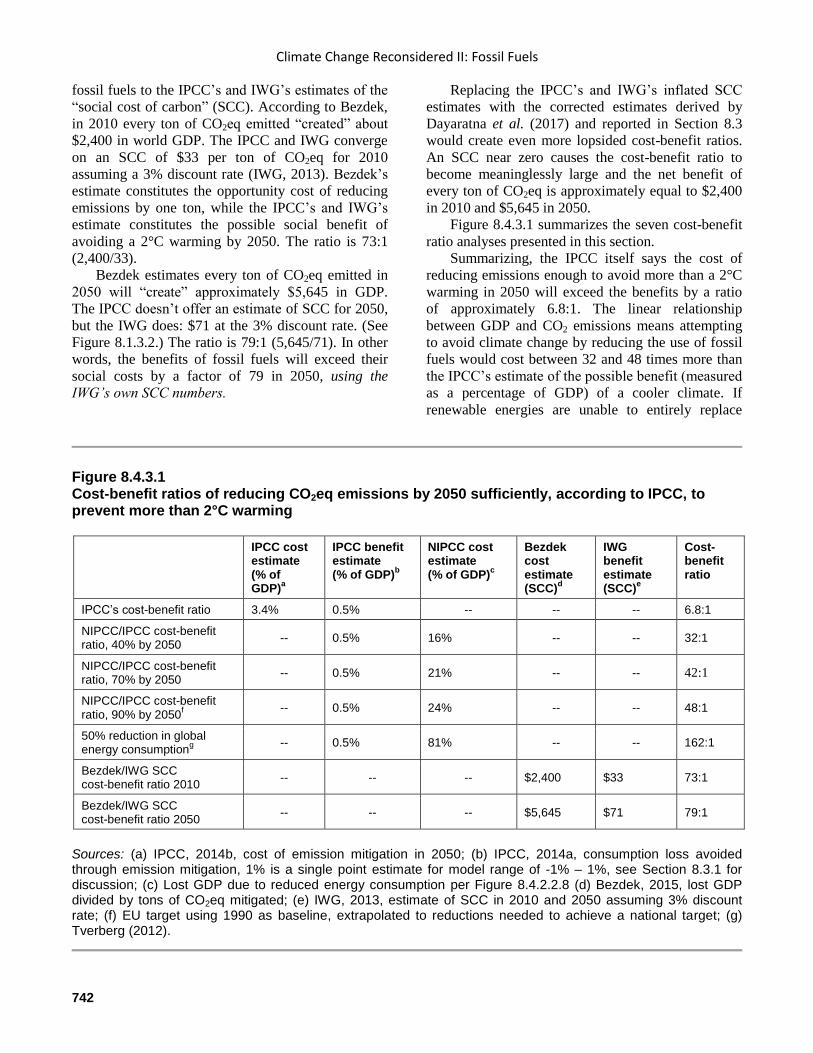
Climate Change Reconsidered II: Fossil Fuels

742

fossil fuels to the IPCC’s and IWG’s estimates of the

“social cost of carbon” (SCC). According to Bezdek,

in 2010 every ton of CO2eq emitted “created” about

$2,400 in world GDP. The IPCC and IWG converge

on an SCC of $33 per ton of CO2eq for 2010

assuming a 3% discount rate (IWG, 2013). Bezdek’s

estimate constitutes the opportunity cost of reducing

emissions by one ton, while the IPCC’s and IWG’s

estimate constitutes the possible social benefit of

avoiding a 2°C warming by 2050. The ratio is 73:1

(2,400/33).

Bezdek estimates every ton of CO2eq emitted in

2050 will “create” approximately $5,645 in GDP.

The IPCC doesn’t offer an estimate of SCC for 2050,

but the IWG does: $71 at the 3% discount rate. (See

Figure 8.1.3.2.) The ratio is 79:1 (5,645/71). In other

words, the benefits of fossil fuels will exceed their

social costs by a factor of 79 in 2050, using the

IWG’s own SCC numbers.

Replacing the IPCC’s and IWG’s inflated SCC

estimates with the corrected estimates derived by

Dayaratna et al. (2017) and reported in Section 8.3

would create even more lopsided cost-benefit ratios.

An SCC near zero causes the cost-benefit ratio to

become meaninglessly large and the net benefit of

every ton of CO2eq is approximately equal to $2,400

in 2010 and $5,645 in 2050.

Figure 8.4.3.1 summarizes the seven cost-benefit

ratio analyses presented in this section.

Summarizing, the IPCC itself says the cost of

reducing emissions enough to avoid more than a 2°C

warming in 2050 will exceed the benefits by a ratio

of approximately 6.8:1. The linear relationship

between GDP and CO2 emissions means attempting

to avoid climate change by reducing the use of fossil

fuels would cost between 32 and 48 times more than

the IPCC’s estimate of the possible benefit (measured

as a percentage of GDP) of a cooler climate. If

renewable energies are unable to entirely replace

Figure 8.4.3.1 Cost-benefit ratios of reducing CO2eq emissions by 2050 sufficiently, according to IPCC, to prevent more than 2°C warming

IPCC cost estimate (% of GDP)

a

IPCC benefit estimate (% of GDP)

b

NIPCC cost estimate (% of GDP)

c

Bezdek cost estimate (SCC)

d

IWG benefit estimate (SCC)

e

Cost-benefit ratio

IPCC’s cost-benefit ratio 3.4% 0.5% -- -- -- 6.8:1

NIPCC/IPCC cost-benefit ratio, 40% by 2050

-- 0.5% 16% -- -- 32:1

NIPCC/IPCC cost-benefit ratio, 70% by 2050

-- 0.5% 21% -- -- 42:1

NIPCC/IPCC cost-benefit ratio, 90% by 2050

f

-- 0.5% 24% -- -- 48:1

50% reduction in global energy consumption

g

-- 0.5% 81% -- -- 162:1

Bezdek/IWG SCC cost-benefit ratio 2010

-- -- -- $2,400 $33 73:1

Bezdek/IWG SCC cost-benefit ratio 2050

-- -- -- $5,645 $71 79:1

Sources: (a) IPCC, 2014b, cost of emission mitigation in 2050; (b) IPCC, 2014a, consumption loss avoided through emission mitigation, 1% is a single point estimate for model range of -1% – 1%, see Section 8.3.1 for discussion; (c) Lost GDP due to reduced energy consumption per Figure 8.4.2.2.8 (d) Bezdek, 2015, lost GDP divided by tons of CO2eq mitigated; (e) IWG, 2013, estimate of SCC in 2010 and 2050 assuming 3% discount rate; (f) EU target using 1990 as baseline, extrapolated to reductions needed to achieve a national target; (g) Tverberg (2012).

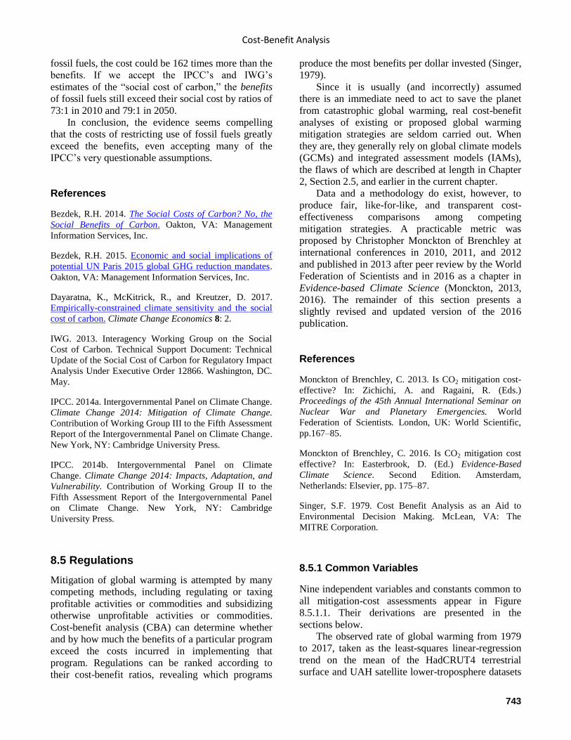
Cost-Benefit Analysis

743

fossil fuels, the cost could be 162 times more than the

benefits. If we accept the IPCC’s and IWG’s

estimates of the “social cost of carbon,” the benefits

of fossil fuels still exceed their social cost by ratios of

73:1 in 2010 and 79:1 in 2050.

In conclusion, the evidence seems compelling

that the costs of restricting use of fossil fuels greatly

exceed the benefits, even accepting many of the

IPCC’s very questionable assumptions.

References

Bezdek, R.H. 2014. The Social Costs of Carbon? No, the

Social Benefits of Carbon. Oakton, VA: Management

Information Services, Inc.

Bezdek, R.H. 2015. Economic and social implications of

potential UN Paris 2015 global GHG reduction mandates.

Oakton, VA: Management Information Services, Inc.

Dayaratna, K., McKitrick, R., and Kreutzer, D. 2017.

Empirically-constrained climate sensitivity and the social

cost of carbon. Climate Change Economics 8: 2.

IWG. 2013. Interagency Working Group on the Social

Cost of Carbon. Technical Support Document: Technical

Update of the Social Cost of Carbon for Regulatory Impact

Analysis Under Executive Order 12866. Washington, DC.

May.

IPCC. 2014a. Intergovernmental Panel on Climate Change.

Climate Change 2014: Mitigation of Climate Change.

Contribution of Working Group III to the Fifth Assessment

Report of the Intergovernmental Panel on Climate Change.

New York, NY: Cambridge University Press.

IPCC. 2014b. Intergovernmental Panel on Climate

Change. Climate Change 2014: Impacts, Adaptation, and

Vulnerability. Contribution of Working Group II to the

Fifth Assessment Report of the Intergovernmental Panel

on Climate Change. New York, NY: Cambridge

University Press.

8.5 Regulations

Mitigation of global warming is attempted by many

competing methods, including regulating or taxing

profitable activities or commodities and subsidizing

otherwise unprofitable activities or commodities.

Cost-benefit analysis (CBA) can determine whether

and by how much the benefits of a particular program

exceed the costs incurred in implementing that

program. Regulations can be ranked according to

their cost-benefit ratios, revealing which programs

produce the most benefits per dollar invested (Singer,

1979).

Since it is usually (and incorrectly) assumed

there is an immediate need to act to save the planet

from catastrophic global warming, real cost-benefit

analyses of existing or proposed global warming

mitigation strategies are seldom carried out. When

they are, they generally rely on global climate models

(GCMs) and integrated assessment models (IAMs),

the flaws of which are described at length in Chapter

2, Section 2.5, and earlier in the current chapter.

Data and a methodology do exist, however, to

produce fair, like-for-like, and transparent cost-

effectiveness comparisons among competing

mitigation strategies. A practicable metric was

proposed by Christopher Monckton of Brenchley at

international conferences in 2010, 2011, and 2012

and published in 2013 after peer review by the World

Federation of Scientists and in 2016 as a chapter in

Evidence-based Climate Science (Monckton, 2013,

2016). The remainder of this section presents a

slightly revised and updated version of the 2016

publication.

References

Monckton of Brenchley, C. 2013. Is CO2 mitigation cost-

effective? In: Zichichi, A. and Ragaini, R. (Eds.)

Proceedings of the 45th Annual International Seminar on

Nuclear War and Planetary Emergencies. World

Federation of Scientists. London, UK: World Scientific,

pp.167–85.

Monckton of Brenchley, C. 2016. Is CO2 mitigation cost

effective? In: Easterbrook, D. (Ed.) Evidence-Based

Climate Science. Second Edition. Amsterdam,

Netherlands: Elsevier, pp. 175–87.

Singer, S.F. 1979. Cost Benefit Analysis as an Aid to

Environmental Decision Making. McLean, VA: The

MITRE Corporation.

8.5.1 Common Variables

Nine independent variables and constants common to

all mitigation-cost assessments appear in Figure

8.5.1.1. Their derivations are presented in the

sections below.

The observed rate of global warming from 1979

to 2017, taken as the least-squares linear-regression

trend on the mean of the HadCRUT4 terrestrial

surface and UAH satellite lower-troposphere datasets

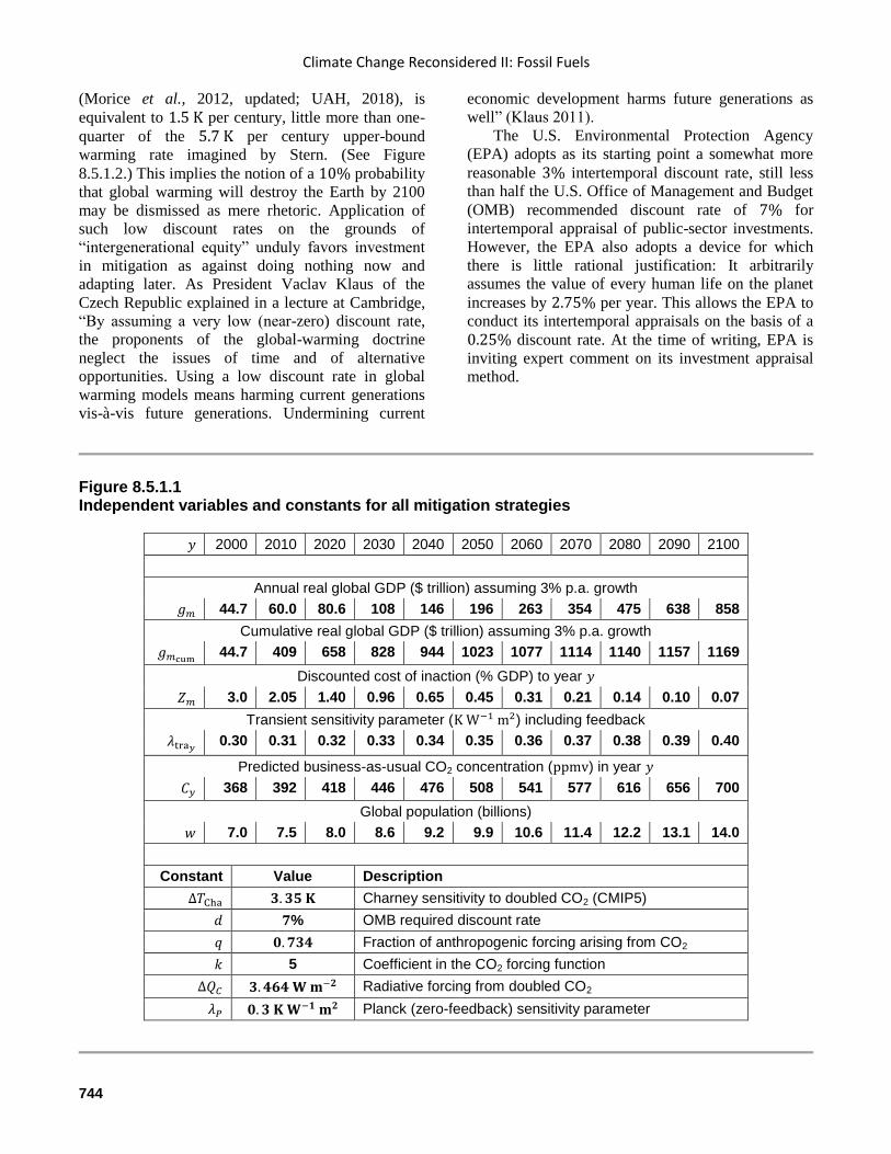
Climate Change Reconsidered II: Fossil Fuels

744

(Morice et al., 2012, updated; UAH, 2018), is

equivalent to 1.5 K per century, little more than one-

quarter of the 5.7 K per century upper-bound

warming rate imagined by Stern. (See Figure

8.5.1.2.) This implies the notion of a 10% probability

that global warming will destroy the Earth by 2100

may be dismissed as mere rhetoric. Application of

such low discount rates on the grounds of

“intergenerational equity” unduly favors investment

in mitigation as against doing nothing now and

adapting later. As President Vaclav Klaus of the

Czech Republic explained in a lecture at Cambridge,

“By assuming a very low (near-zero) discount rate,

the proponents of the global-warming doctrine

neglect the issues of time and of alternative

opportunities. Using a low discount rate in global

warming models means harming current generations

vis-à-vis future generations. Undermining current

economic development harms future generations as

well” (Klaus 2011).

The U.S. Environmental Protection Agency

(EPA) adopts as its starting point a somewhat more

reasonable 3% intertemporal discount rate, still less

than half the U.S. Office of Management and Budget

(OMB) recommended discount rate of 7% for

intertemporal appraisal of public-sector investments.

However, the EPA also adopts a device for which

there is little rational justification: It arbitrarily

assumes the value of every human life on the planet

increases by 2.75% per year. This allows the EPA to

conduct its intertemporal appraisals on the basis of a

0.25% discount rate. At the time of writing, EPA is

inviting expert comment on its investment appraisal

method.

Figure 8.5.1.1 Independent variables and constants for all mitigation strategies

𝑦 2000 2010 2020 2030 2040 2050 2060 2070 2080 2090 2100

Annual real global GDP ($ trillion) assuming 3% p.a. growth

𝑔𝑚 44.7 60.0 80.6 108 146 196 263 354 475 638 858

Cumulative real global GDP ($ trillion) assuming 3% p.a. growth

𝑔𝑚cum 44.7 409 658 828 944 1023 1077 1114 1140 1157 1169

Discounted cost of inaction (% GDP) to year 𝑦

𝑍𝑚 3.0 2.05 1.40 0.96 0.65 0.45 0.31 0.21 0.14 0.10 0.07

Transient sensitivity parameter (K W−1 m2) including feedback

𝜆tra𝑦 0.30 0.31 0.32 0.33 0.34 0.35 0.36 0.37 0.38 0.39 0.40

Predicted business-as-usual CO2 concentration (ppmv) in year 𝑦

𝐶𝑦 368 392 418 446 476 508 541 577 616 656 700

Global population (billions)

𝑤 7.0 7.5 8.0 8.6 9.2 9.9 10.6 11.4 12.2 13.1 14.0

Constant Value Description

∆𝑇Cha 𝟑. 𝟑𝟓 𝐊 Charney sensitivity to doubled CO2 (CMIP5)

𝑑 𝟕% OMB required discount rate

𝑞 𝟎. 𝟕𝟑𝟒 Fraction of anthropogenic forcing arising from CO2

𝑘 5 Coefficient in the CO2 forcing function

∆𝑄𝐶 𝟑. 𝟒𝟔𝟒 𝐖 𝐦−𝟐 Radiative forcing from doubled CO2

𝜆𝑃 𝟎. 𝟑 𝐊 𝐖−𝟏 𝐦𝟐 Planck (zero-feedback) sensitivity parameter

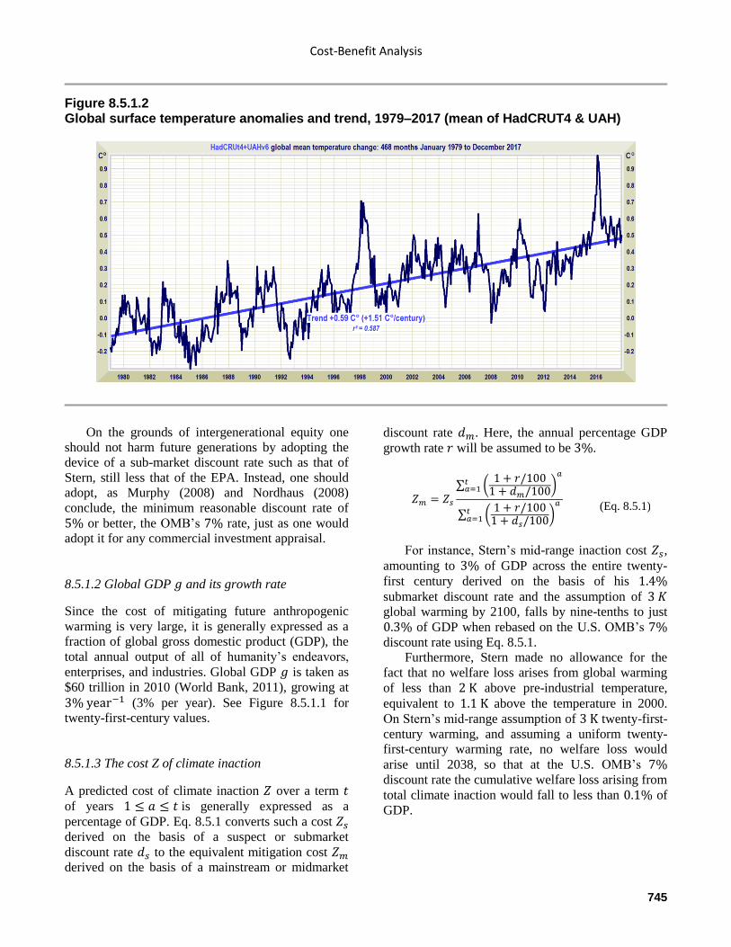
Cost-Benefit Analysis

745

Figure 8.5.1.2 Global surface temperature anomalies and trend, 1979–2017 (mean of HadCRUT4 & UAH)

On the grounds of intergenerational equity one

should not harm future generations by adopting the

device of a sub-market discount rate such as that of

Stern, still less that of the EPA. Instead, one should

adopt, as Murphy (2008) and Nordhaus (2008)

conclude, the minimum reasonable discount rate of

5% or better, the OMB’s 7% rate, just as one would

adopt it for any commercial investment appraisal.

8.5.1.2 Global GDP 𝑔 and its growth rate

Since the cost of mitigating future anthropogenic

warming is very large, it is generally expressed as a

fraction of global gross domestic product (GDP), the

total annual output of all of humanity’s endeavors,

enterprises, and industries. Global GDP 𝑔 is taken as

$60 trillion in 2010 (World Bank, 2011), growing at

3% year−1 (3% per year). See Figure 8.5.1.1 for

twenty-first-century values.

8.5.1.3 The cost Z of climate inaction

A predicted cost of climate inaction 𝑍 over a term 𝑡

of years 1 ≤ 𝑎 ≤ 𝑡 is generally expressed as a

percentage of GDP. Eq. 8.5.1 converts such a cost 𝑍𝑠

derived on the basis of a suspect or submarket

discount rate 𝑑𝑠 to the equivalent mitigation cost 𝑍𝑚

derived on the basis of a mainstream or midmarket

discount rate 𝑑𝑚. Here, the annual percentage GDP

growth rate 𝑟 will be assumed to be 3%.

𝑍𝑚 = 𝑍𝑠

∑ (1 + 𝑟/100

1 + 𝑑𝑚/100)

𝑎𝑡𝑎=1

∑ (1 + 𝑟/100

1 + 𝑑𝑠/100)

𝑎𝑡𝑎=1

(Eq. 8.5.1)

For instance, Stern’s mid-range inaction cost 𝑍𝑠,

amounting to 3% of GDP across the entire twenty-

first century derived on the basis of his 1.4%

submarket discount rate and the assumption of 3 𝐾

global warming by 2100, falls by nine-tenths to just

0.3% of GDP when rebased on the U.S. OMB’s 7%

discount rate using Eq. 8.5.1.

Furthermore, Stern made no allowance for the

fact that no welfare loss arises from global warming

of less than 2 K above pre-industrial temperature,

equivalent to 1.1 K above the temperature in 2000.

On Stern’s mid-range assumption of 3 K twenty-first-

century warming, and assuming a uniform twenty-

first-century warming rate, no welfare loss would

arise until 2038, so that at the U.S. OMB’s 7%

discount rate the cumulative welfare loss arising from

total climate inaction would fall to less than 0.1% of

GDP.

Climate Change Reconsidered II: Fossil Fuels

746

8.5.1.4 Charney sensitivity ∆𝑇𝐶ℎ𝑎

The standard metric for projecting anthropogenic

global warming is Charney sensitivity ∆𝑇Cha; i.e.,

climate sensitivity to a doubling of atmospheric CO2

concentration. Charney (1979) held that his

eponymous sensitivity was 3.0 [1.5, 4.5] K, the value

adopted by IPCC (1990) and, with little change, in all

subsequent Assessment Reports. In the third-

generation (CMIP3) and fifth-generation (CMIP5)

models of the Climate Model Intercomparison

Project, Charney sensitivity was thought to be

3.35 [2.1, 4.7] K (Andrews et al., 2012). Predicted

global warming from all anthropogenic sources over

the twenty-first century tends to be approximately

equal to Charney sensitivity. Here, the CMIP3/5 mid-

range estimate 3.35 K will be assumed arguendo to

be normative.

8.5.1.5 The CO2 fraction 𝑞

IPCC (2013, Fig. SPM.5) finds that, of the

2.29 W m−2 net anthropogenic forcing to 2011,

1.68 W m−2 is attributable to CO2. Accordingly, the

CO2 fraction 𝑞 = 1.68/2.29 = 0.734.

8.5.1.6 The CO2 radiative forcing ∆𝑄𝐶

Andrews et al. (2012), reviewing an ensemble of two

dozen CMIP5 models, provides data on the basis of

which one may conclude that the radiative forcing

∆𝑄𝐶 in response to doubled CO2 concentration is

3.464 W m−2. On the interval of interest, the CO2

forcing function is approximately logarithmic. Thus,

∆𝑄𝐶 = 𝑘 ln (𝐶1/𝐶0), where 𝐶0 is the unperturbed

concentration (Myhre et al., 1998; IPCC, 2001,

Section 6.1). Thus, 𝑘 = 3.464/ ln 2 = 5.

8.5.1.7 The Planck sensitivity parameter 𝜆𝑃

The Planck sensitivity parameter 𝜆𝑃, the quantity by

which a radiative forcing Δ𝑄𝐸 in Watts per square

meter is multiplied to yield a temperature change Δ𝑇𝑆

before accounting for temperature feedback, is the

first derivative Δ𝑇𝑆/Δ𝑄𝐸 = 𝑇𝑆/(4𝑄𝐸) of the

fundamental equation of radiative transfer. Surface

temperature 𝑇𝑆 = 288.4 K (ISCCP, 2018). Given

total solar irradiance 𝑆0 = 1364.625 W m−2

(Mekaoui et al., 2010) and albedo 𝛼 = 0.293 (Loeb

et al., 2009), radiative flux density 𝑄𝐸 = 𝑆0(1 −

𝛼)/4 = 241.2 W m−2 at the mean emission altitude.

Therefore, 𝜆𝑃 is today equal to 0.30 K W−1 m2

(Schlesinger, 1985).

8.5.1.8 The transient-sensitivity parameter 𝜆𝑡𝑟𝑎

IPCC (2007, Table SPM.3) gives predicted transient

anthropogenic forcings Δ𝑄tra and warmings Δ𝑇tra

from 1900 to 2100 for six scenarios. On all six

scenarios, the bicentennial transient-sensitivity

parameter 𝜆bi, which exceeds 𝜆𝑃 to the extent that

some temperature feedbacks have acted, is

0.5 K W−1 m2 (see IPCC 2001, p. 354, citing

Ramanathan, 1985).

An appropriate twenty-first-century centennial

value 𝜆tra is the mean of 𝜆𝑃 and 𝜆bi; i.e.,

0.4 K W−1 m2, in agreement with Garnaut (2008),

who wrote of keeping greenhouse-gas increases to

450 ppmv CO2 equivalent above the 280 ppmv

prevalent in 1750 with the aim of holding twenty-

first-century global warming to 2 K, implying

𝜆tra = 0.4 K W−1 m2. Values of Δ𝑇tra implicit in this

value of 𝜆tra are shown in Figure 8.5.1.1.

8.5.1.9 Global population 𝑤

Global population 𝑤 is here taken as 7 billion (bn) in

2000, rising exponentially to 14 bn in 2100.

References

Andrews, T., Gregory, J.M., Webb, M.J., and Taylor, K.E.

2012. Forcing, feedbacks and climate sensitivity in CMIP5

coupled atmosphere-ocean climate models. Geophysical

Research Letters 39: L09712.

Charney, J.G., et al. 1979. Carbon Dioxide and Climate: A

Scientific Assessment. Report of an Ad-Hoc Study Group

on Carbon Dioxide and Climate, Climate Research Board,

Assembly of Mathematical and Physical Sciences, and

National Research Council. Washington, DC: National

Academies of Sciences.

Dietz, S., Hope, C., Stern, N., and Zenghelis, D. 2007.

Reflections on the Stern Review (1): a robust case for

strong action to reduce the risks of climate change. World

Economics 8 (1): 121–68.

Garnaut, R. 2008. The Garnaut Climate Change Review:

Final Report. Port Melbourne, Australia: Cambridge

University Press.

Cost-Benefit Analysis

747

Garnaut, R. 2011. The Garnaut Review 2011: Australia in

the Global Response to Climate Change. Cambridge, UK:

Cambridge University Press.

Green Book. 2018. The Green Book: Appraisal and

Evaluation in Central Government: Treasury Guidance.

London, UK: HM Treasury.

IPCC. 1990. Intergovernmental Panel on Climate Change.

Climate Change – The IPCC Assessment (1990). Report

prepared for the Intergovernmental Panel on Climate

Change by Working Group I. Cambridge, , UK:

Cambridge University Press.

IPCC. 2001. Intergovernmental Panel on Climate Change.

Climate Change 2001: The Scientific Basis. Contribution

of Working Group I to the Third Assessment Report of the

Intergovernmental Panel on Climate Change. Cambridge,

UK: Cambridge University Press.

IPCC. 2007. Intergovernmental Panel on Climate Change.

Climate Change 2007: the Physical Science Basis.

Contribution of Working Group I to the Fourth

Assessment Report of the Intergovernmental Panel on

Climate Change. Cambridge, UK: Cambridge University

Press.

IPCC. 2013. Intergovernmental Panel on Climate Change.

Climate Change 2013: The Physical Science Basis.

Contribution of Working Group I to the Fifth Assessment

Report of the Intergovernmental Panel on Climate Change.

Cambridge, UK: Cambridge University Press.

ISCCP. 2018. Cloud analysis (part I): Climatology of

global cloud and surface properties (website). Accessed

May 25, 2018.

Klaus, V. 2011. The Global Warming Doctrine Is Not a

Science. Conference on The Science and Economics of

Climate Change. Cambridge, UK: Downing College. May.

Loeb, G.N., Wielicki, B.A., Dölling, D.R., Smith, G.L.,

Keyes, D.F., Kato, S., Manalo-Smith, N., and Wong, T.,

2009. Toward optimal closure of the Earth’s top-of-

atmosphere radiation budget. Journal of Climate 22: 748–

66.

Mekaoui, S., Dewitte S., Conscience, C., and Chevalier A.

2010. Total solar irradiance absolute level from

DIRAD/SOVIM on the International Space Station.

Advanced Space Research 45: 1393–1406.

Murphy, K.M. 2008. Some Simple Economics of Climate

Changes. Paper presented to the Mont Pelerin Society

General Meeting, Tokyo. September 8.

Lowe, J. 2008. Intergenerational Wealth Transfers and

Social Discounting: Supplementary Green Book Guidance.

London, UK: HM Treasury.

Morice, C.P., Kennedy, J.J., Rayner, N., and Jones, P.D.

2012 Quantifying uncertainties in global and regional

temperature change using an ensemble of observational

estimates: the HadCRUT4 dataset. Journal of Geophysical

Research 117:D08101.

Myhre, G., et al., 1998. New estimates of radiative forcing

due to well mixed greenhouse gases. Geophysical

Research Letters 25 (14): 2715–8.

Nordhaus, W.D. 2008. A Question of Balance: Weighing

the Options on Global Warming Policies. New Haven, CT:

Yale University Press.

Ramanathan, V., et al. 1985. Trace gas trends and their

potential role in climate change. Journal of Geophysical

Research 90: 5547–66.

Schlesinger, M.E. 1985. Feedback analysis of results from

energy balance and radiative-convective models. In: The

Potential Climatic Effects of Increasing Carbon Dioxide.

MacCracken, M.C. and Luther, F.M. (Eds,). Washington,

DC: U.S. Department of Energy, 280–319.

Stern, N., et al. 2007. The Economics of Climate Change:

The Stern Review. Cambridge, UK: Cambridge University

Press.

UAH. 2018. Monthly global mean land and sea lower-

troposphere temperature anomalies. (website). Accessed

November 19, 2018.

World Bank. 2011. Gross Domestic Product 2009, World

Development Indicators.

8.5.2 Case-specific variables

Only three case-specific inputs are required and are

described below.

8.5.2.1 The discounted cost 𝑋𝑚

The cost 𝑋𝑚 of a given mitigation strategy is

discounted to present value at the chosen market

intertemporal discount rate 𝑑𝑚.

8.5.2.2 The business-as-usual CO2 concentration 𝐶𝑦

The currently predicted business-as-usual CO2

concentration 𝐶𝑦 in the target final year 𝑦2 of any

existing or proposed mitigation strategy is given in

Figure 8.5.1.1, allowing ready derivation of an

appropriate value for any year of the twenty-first

Climate Change Reconsidered II: Fossil Fuels

748

century. CO2 concentration in the twenty-first century

is extrapolated from trends in Tans (2011) and

Conway & Tans (2011) according to the mid-range

estimates in IPCC (2007, 2013), by which CO2

increases exponentially from 368 ppmv in 2000 to

700 ppmv in 2100.

This value is the benchmark against which any

foreseeable reduction in CO2 concentration achieved

by the mitigation strategy is measured. It will be seen

from the case studies that such reductions are in

practice negligible.

8.5.2.3 The fraction 𝑝 of global business-as-usual

CO2 emissions the strategy will abate

The fraction 𝑝 of projected global business-as-usual

CO2 emissions until year 𝑦2 that will be abated under

the (usually generous) assumption that the strategy

will work as advertised is an essential quantity that is

seldom derived in any integrated assessment model.

References

Conway, T. and Tans, P. 2011, Recent trends in globally-

averaged CO2 concentration, NOAA/ESRL (website).

Accessed November 19, 2018.

IPCC. 2007. Intergovernmental Panel on Climate Change.

Climate Change 2007: the Physical Science Basis.

Contribution of Working Group I to the Fourth

Assessment Report of the Intergovernmental Panel on

Climate Change. Cambridge, UK: Cambridge University

Press.

IPCC. 2013. Intergovernmental Panel on Climate Change.

Climate Change 2013: The Physical Science Basis.

Contribution of Working Group I to the Fifth Assessment

Report of the Intergovernmental Panel on Climate Change.

Cambridge, UK: Cambridge University Press.

Tans, P. 2011. NOAA global monthly mean CO2

concentration trends dataset (website). Accessed

November 19, 2018.

8.5.3 Outputs

A robust cost-benefit model comprising a system of

simple equations informed by the independent

variables described in Sections 8.5.1 and 8.5.2 may

readily be applied to any given mitigation strategy.

The model can produce three outputs.

8.5.3.1 The unit mitigation cost 𝑀

Unit mitigation cost 𝑀 is here defined as the cost of

abating 1 K global warming on the assumption that

all measures to abate anthropogenic warming to year

𝑦 have a cost-effectiveness identical to the strategy

under consideration.

8.5.3.2 Global abatement cost 𝐻 per capita and 𝐽 as

% GDP.

On the same assumption, the strategy’s global

abatement cost is the total cost of abating all

predicted global warming ∆𝑇𝐶21 (see Figure 8.5.1.1)

over the term 𝑡 from year 𝑦1 to year 𝑦2. This global

abatement cost may be expressed in three ways: as a

global cash cost 𝑋𝑑, as a cost 𝐻 per head of global

population, and as a percentage 𝐽 of global GDP over

the term 𝑡.

8.5.3.3 The benefit/cost or action/inaction ratio 𝐴

Finally, the benefit/cost or action/inaction ratio 𝐴 of

the chosen mitigation strategy is the ratio of the GDP

cost 𝐽 of implementation to the GDP cost 𝑍𝑑 of

inaction now and adaptation later.

8.5.4 Cost-benefit Model

The purpose of the model is to give policymakers

unfamiliar with climatology a simple but focused and

robust method of answering two questions: how the

cost of an existing or proposed mitigation strategy

compares with those of competing strategies, and

whether that cost exceeds the cost of not mitigating

global warming at all.

The model comprises the following sequence of

equations designed to be readily programmable. The

model is so simple that it can be run on a pocket

calculator. Yet, because it is rooted in mainstream

climate science, it will give a more focused and

reliable indication of the costs and benefits of

individual mitigation strategies than any integrated

assessment model.

Where 𝑝, on [0, 1], is the fraction of future global

emissions that a mitigation strategy is projected to

abate by a target calendar year 𝑦2, and 𝐶y2 is the

IPCC’s projected unmitigated CO2 concentration in

year 𝑦2, model Eq. M1 gives 𝐶mit, the somewhat

lesser concentration in ppmv that is expected to

Cost-Benefit Analysis

749

obtain in year 𝑦2 if the strategy is successfully

followed.

𝐶mit = 𝐶y2 − 𝑝(𝐶y2 − 𝐶y1) M1

The CO2 forcing equation is model Eq. M2,

where 𝐶0 is the unperturbed concentration.

∆𝑄𝐶 = 𝑘 ln(𝐶1/𝐶0) = 5 ln(𝐶1/𝐶0). M2

Accordingly, the CO2 forcing ∆𝑄aba abated by

the chosen strategy is given by Eq. M3.

∆𝑄aba = 5 ln(𝐶𝑦2/𝐶mit). M3

Then the global warming abated by the

mitigation strategy to the final year 𝑦2 is given by Eq.

M4. ∆𝑇aba = 𝜆tra𝑦2

𝑘 [ln(𝐶𝑦2/𝐶𝑦1)

− ln(𝐶mit/𝐶y1)]

M4

= 5 𝜆tra𝑦2 ln(𝐶y2/𝐶mit).

The unit mitigation cost 𝑀 is given by Eq. M5,

and the predicted global warming ∆𝑇𝑦2 over the term

is given by Eq. M6,

𝑀 = 𝑋𝑚/∆𝑇aba; M5

∆𝑇𝑦2 = 5 𝜆tra𝑦2 ln (𝐶𝑦2/𝐶𝑦1). M6

The global abatement costs 𝐺 in cash, 𝐻 per

capita and 𝐽 as a percentage of global GDP of abating

all predicted global warming ∆𝑇𝑦2 over the term 𝑡 of

the strategy are given by Eqs. M7–M9, where 𝑤 is

global population, 𝐺 is the real cumulative

discounted cost of abating ∆𝑇𝑦2, and 𝑍𝑚 is the real

cumulative discounted cost of inaction over the same

term.

𝐺 = 𝑀 ∆𝑇𝑦2. M7

𝐻 = 𝐺/𝑤. M8

𝐽 = 100 𝐺/𝑍𝑚. M9

Finally, the benefit-cost or action-inaction ratio 𝐴

is given by Eq. M10, where 𝐴 is the ratio of the

cumulative discounted GDP cost 𝐽 of the strategy

over the term to the cumulative discounted cost of

inaction as a percentage of GDP over the term.

𝐴 = 𝐽/𝑍𝑚. M10

8.5.5 Model Applied

8.5.5.1 2009 U.S. Cap-and-Trade Bill

In the United States in 2009, Democrats tried and

failed to pass a “cap-and-trade” bill (HR 2454, SB

311) its sponsors said would cost $180 bn per year

for 40 years, or $7.2 tn in all, which is here

discounted by 7% yr−1 to $2.6 tn at present value.

The stated aim of the bill was to abate 83% of U.S.

CO2 emissions by 2050. Since the U.S. emitted 17%

of global CO2 at the time (derived from Olivier and

Peters, 2010, Table A1), the fraction of global CO2

emissions abated would have been 0.14. The

business-as-usual CO2 concentration in 2050 would

be 508 ppmv without the bill and 492 ppmv (from

Eq. M1) with it, whereupon radiative forcing abated

would have been 0.16 W m–2

(Eq. M3) and global

warming abated over the 40-year term would have

been less than 0.06 K (Eq. M4).

Accordingly, the unit cost of abating 1 K global

warming by measures of cost-ineffectiveness

equivalent to the bill would have been equal to the

ratio of the discounted cost to the warming averted;

i.e., $46 tn K−1 per Kelvin (Eq. M5). Therefore, the

cash cost of abating all of the predicted 0.44 K global

warming (Eq. M6) from 2011 to 2050 would have

been more than $20 tn; or more than $2000 per head

of global population, man, woman, and child; or

3.3% of cumulative discounted global GDP over the

term. The action/inaction ratio would then be the

ratio of the 3.3% GDP cost of action to the 0.45%

GDP cost of inaction to 2050, i.e. 7.4: 1.

Implementing the cap-and-trade bill, or measures of

equivalent unit mitigation cost, would have been

almost seven and a half times costlier than the cost of

doing nothing now and adapting to global warming

later – always supposing that the cost of any such

adaptation were to exceed the benefit of warmer

weather and more CO2 fertilization worldwide.

Additional case studies are briefly summarized in

Sections 8.5.5.2–8.5.5.9. Section 8.5.6 draws lessons

from the results delivered by the cost-benefit model.

8.5.5.2 The UK’s Climate Change Act

In 2008, the British parliament approved the Climate

Change Act of 2008. The cost stated in the

government’s case was $39.4 bn yr−1 for 40 years,

which, discounted at 7% yr−1 to present value,

would be $526 bn. The aim was to cut national

Climate Change Reconsidered II: Fossil Fuels

750

emissions by 80% over the term.

Since UK emissions are only 1.5% of global

emissions, the fraction of global emissions abated

will be 0.012. CO2 concentration by 2050 would

have been 508 ppmv without the bill and will be

506 ppmv with it. Anthropogenic forcing abated

over the term will be 0.013 W m−2, and warming

abated will be 0.005 K. Unit mitigation cost will thus

be $526 bn / 0.005, or $112 tn K−1. The cash cost

of abating all of the predicted 0.44 K warming over

the term will be $49.5 tn; the cost per head of global

population will be $5000, or 8% of GDP over the

term. The action-inaction ratio is 18: 1.

8.5.5.3 The European Union’s carbon trading

scheme

EU carbon trading costs $92 bn yr−1 (World Bank

2009, p. 1), here multiplied by 2.5 (implicit in

Lomborg, 2007) to allow for numerous non-trading

mitigation measures. Total cost is $2.3 tn over the

10-year term to 2020, or $1.6 tn at present value. The

declared aim of the EU scheme was to abate 20% of

member states’ emissions, which were 13% of global

emissions (from Boden et al., 2010a, 2010b). Thus,

the fraction of global emissions abated will be 0.026.

CO2 emissions in 2020 will be 419 ppmv without the

EU scheme and 418 ppmv with it. Radiative forcing

abated is thus just 0.007 W m−2, and warming

abated is 0.002 K.

Accordingly, the unit mitigation cost of the EU’s

carbon trading scheme is $690 tn K−1, and the cash

cost of abating the < 0.1 K warming predicted to

occur over the 10-year term is $64 tn; or $8000 per

head of global population; or 26% of global GDP.

Acting on global warming by measures of equivalent

unit mitigation cost would be 18 times costlier than

doing nothing now and adapting later.

8.5.5.4 California’s cap-and-trade Act

Under AB32 (2006), which came fully into effect in

2012, some $182 bn yr−1 (Varshney and Tootelian,

2009) will be spent in the 10 years to 2021 on cap

and trade and related measures. The gross cost is thus

$1.8 tn, discounted to $1.3 tn. California’s stated aim

was to reduce its emissions, which represent 8% of

U.S. emissions, by 25%. U.S. emissions at the

beginning of the scheme were 17% of global

emissions: thus, the fraction of global emissions

abated will be 0.0033. CO2 concentration will fall

from a business-as-usual 421 ppmv to just under

421 ppmv by 2021. Anthropogenic forcing abated

will be 0.001 W m−2, and warming abated will be

less than one-thousandth of a Kelvin.

Accordingly, unit mitigation cost of California’s

cap-and-trade program will approach $4 quadrillion

per °K of global warming avoided; cost per head will

be $43,000, or almost 150% of global GDP over the

term. It will be well more than 100 times costlier to

mitigate global warming by measures such as this

than to take no measures at all and adapt to such

warming as may occur.

8.5.5.5 The Thanet wind array

Subsidy to one of the world’s largest wind turbine

installations, off the English coast, is guaranteed at

$100 million annually for its 20-year lifetime; i.e.

$1.06 bn at present value. Rated output of the 100

turbines is 300 MW, but such installations yield only

24% of rated capacity (Young, 2011, p. 1), so total

output, at 72 MW, is only 1/600 of mean 43.2 GW

UK electricity demand (Department for Energy and

Climate Change, 2011). Electricity accounts for one-

third of U.K. emissions, which represent 1.5% of

global emissions. Therefore, the fraction of global

emissions abated over the 20-year period will be

8.333 x 10−6. Business-as-usual CO2 concentration

in 2030 would be 446.296 ppmv without the array,

falling to 446.2955 ppmv with it. Forcing abated is

0.000005 W m−2, so that warming abated is less

than 0.000002 K.

Accordingly, the unit mitigation cost of the

Thanet wind array is $670 tn K−1. To abate the

predicted 0.2 K warming over the 20-year term, the

cost in cash would be $135 tn; per head $16,000;

and almost one-third of global GDP over the term. It

would be 34 times costlier to act on global warming

than to do nothing today and adapt later.

8.5.5.6 Australia’s carbon trading scheme

Australia’s 2011 Clean Energy Act cost

$10.1 bn yr−1, plus $1.6 bn yr−1 for administration

(Wong 2010, p. 5), plus $1.2 bn yr−1 for renewables

and other costs, a total of $13 bn yr−1, rising at

5% yr−1, giving a total discounted cost of $117 bn

at present value. The stated aim of the legislation was

to reduce Australia’s CO2 emissions by 5% over the

Cost-Benefit Analysis

751

term. Australia’s emissions represent 1.2% of global

emissions (derived from Boden and Marland, 2010;

Boden et al., 2010). Thus the fraction of global

emissions abated is 0.0006. CO2 concentration would

fall from a business-as-usual 418.5 ppmv without the

Australian scheme to 418.49 ppmv with it, so that

warming of 0.00005 K would be abated.

The unit mitigation cost of Australia’s carbon

trading scheme would be $2.2 quadrillion per Kelvin.

To abate the 0.1 K warming predicted for the period

(the warming did not occur) would be $201 tn. The

cost per head would exceed $25,000, or 81% of

global GDP throughout the term. The cost of acting

on climate change by measures such as Australia’s

scheme would approach 60 times that of inaction.

8.5.5.7 Gesture politics 1: a wind turbine on an

elementary school roof in England

On March 31, 2010, Sandwell Council in England

answered a freedom-of-information request

(McCauley, 2011) by disclosing that it had spent

£5875 ($7730) on buying and installing a small

wind turbine capable of generating 209 KWh in a

year – enough to power a single 100 W reading-lamp

for less than three months. The fraction of UK

emissions abated by the wind turbine is 33% of

209 KWh / 365 days / 24 hr / 43.2 GW, or

0.00000002%, and, since UK emissions are only

1.5% of global emissions, the fraction of global

emissions abated is less than 0.000000000003.

Forcing abated is < 0.000000000002 W m−2.

Warming abated is 0.0000000000005 K.

The unit mitigation cost of a wind turbine on an

elementary school roof in England is $14.5

quadrillion per Kelvin. To abate all of the 0.2 K

global warming predicted to occur over the 20-year

life of the wind turbine, the cost is $3 quadrillion, or

$340 tn per head, or 700% of GDP. Action costs

more than 730 times inaction.

8.5.5.8 Gesture politics 2: Maryland’s 90% cut in

CO2 emissions

In the United States, the state of Maryland’s

government decided that from 2011 to 2050 it would

reduce its CO2 emissions by 90% at a discounted

cost of $7.3 tn, about three times the discounted cost

of the rejected national cap-and-tax scheme over the

same period. The reduction would have amounted to

1.5% of national emissions, which are 17% of global

emissions. Therefore, the fraction of global emissions

abated is 0.0025. The predicted business-as-usual

CO2 concentration of 507.55 ppmv would fall to

507.25 ppmv. Radiative forcing abated is less than

0.003 W m−2, and warming abated is 0.001 K.

The unit mitigation cost is $7.3 quadrillion. The

cost of abating the predicted 0.44 K global warming

over the period is $3 quadrillion, or $320,000 per

head of global population, or well more than 500%

of global GDP over the period. Attempted mitigation

by measures as costly as Maryland’s scheme would

be 1150 times costlier than inaction today and

adaptation later.

8.5.5.9 Gesture politics 3: The London bicycle-hire

scheme

Perhaps the costliest measure ever adopted in the

name of abating global warming was the London

bicycle-hire scheme, which cost $130 bn upfront,

together with large annual maintenance costs that are

not included here, for just 5000 bicycles – a cost of

$26,000 per bicycle. Transport represents 15.2% of

UK emissions (from Office for National Statistics,

2010, Table C). Cycling represents 3.1 bn of the

316.3 bn vehicle miles traveled on UK roads

annually (Department for Transport, 2011). There are

23 million bicycles in use in Britain (Cyclists’

Touring Club, 2011).

Global emissions will be cut by 1.5% of 15.2%

of 3.1/316.3 x 5000/23,000,000. Thus the fraction

of global emissions abated will be 4.886 x 10−9. If

the lifetime of bicycles and docking stations is 20

years, business-as-usual CO2 concentration of

446.296 ppmv will fall to 446.2989 ppmv through

the scheme. Forcing abated is 0.000000003 W m−2;

warming abated is 0.000000001 𝐾; unit mitigation

cost exceeds $141 quadrillion per Kelvin abated; and

the cash global abatement cost of $28.5 quadrillion is

$3.3 million per head, or almost 7000% of global

GDP to 2030. Action costs more than 7000 times

inaction.

References

AB 32. 2006. Global Warming Solutions Act. Sacramento,

CA: California State Legislature.

Boden, T. and Marland, G. 2010. Global CO2 Emissions

from Fossil-Fuel Burning, Cement Manufacture, and Gas

Climate Change Reconsidered II: Fossil Fuels

752

Flaring, 1751-2007. Oak Ridge, TN: Carbon Dioxide

Information and Analysis Center.

Boden, T. et al. 2010. Ranking of the world’s countries by

2007 total CO2 emissions from fossil-fuel burning, cement

production, and gas flaring. Oak Ridge, TN: Carbon

Dioxide Information and Analysis Center.

Clean Energy Bill. 2011. Exposure Draft. Parliament of the

Commonwealth of Australia, 2011.

Climate Change Act. 2008. London, UK: HM Stationery

Office.

Cyclists’ Touring Club. 2011. Cyclists’ Touring Club

Facts and Figures (website).

Department for Energy and Climate Change. 2011. UK

Energy Statistics: Electricity (website).

Department for Transport. 2011. Table TRA0101, Road

Traffic by Vehicle Type, Great Britain, 1950–2009

(website).

HR 2454. 2009. American Clean Energy & Security Bill.

111th

Congress, Washington DC.

Lomborg, B. 2007. Perspective on Climate Change.

Testimony before the Committee on Science and

Technology of the U.S. House of Representatives. March

21.

McCauley, R. 2011. Letter of response to a request under

the Freedom of Information Act received from Peter Day.

Oldbury, UK: Sandwell Borough Council. March 31.

Office for National Statistics. 2010. Statistical Bulletin:

Greenhouse Gas Emissions Intensity Falls in 2008.

Newport, UK: Office for National Statistics.

Olivier, J.G.J. and Peters, J.A.H.W. 2010. Mondiale

emissies koolstofdioxide door gebruik fossiele

brandstoffen en cementproductie [Global emissions of

carbon dioxide by using fossil fuels and cement

production], 1990–2009. The Hague, Netherlands: PBL

Netherlands Environmental Assessment Agency.

Varshney, S.B. and Tootelian, D.H. 2009. Cost of AB 32

on California Small Businesses. Sacramento, CA:

California Small Business Roundtable.

Wong, P. 2010. Portfolio Budget Statements 2010–11:

Budget-Related Paper No. 1.4. Climate Change and

Energy Efficiency Portfolio. Canberra, Australia:

Commonwealth of Australia.

World Bank. 2009. State and Trends of the Carbon

Market. Washington, DC.

Young, S. 2011. Analysis of UK Wind Power Generation,

November 2008 to December 2010. Edinburgh, Scotland:

John Muir Trust. March.

8.5.6 Results Discussed

For the sake of simplicity and accessibility, the focus

of the method is deliberately narrow. Potential

benefits external to CO2 mitigation, changes in global

warming potentials, variability in the global GDP

growth rate, or relatively higher mitigation costs in

regions with lower emission intensities are ignored,

for little error arises. GDP growth rates and climate-

inaction costs are assumed uniform, though in

practice little climate-related damage would arise

unless global temperature rose by at least 1 K above

today’s temperatures. Given the small amount of

warming abated by CO2-reduction strategies, as well

as the breadth of the intervals of published estimates

of inaction and mitigation costs, modeling non-

uniform GDP growth rates and climate-inaction costs

may in any event prove irrelevant.

Government predictions of abatement costs

(cases 1 and 2) are of the same order as those in Stern

(2006) and Garnaut (2008) and the reviewed

literature. However, the costs of specific measures

(cases 3 through 6) prove significantly higher than

official predictions. Gesture policies (cases 7 through

9) are absurdly costly and are studied here because

there are so many of them. These results indicate

there is no rational economic case for global warming

mitigation. The arguments for mitigation are,

therefore, solely political.

Mitigation is so much costlier than adaptation

that real and substantial damage is being done to

Western economic interests. Though the cost-benefit

model concentrates exclusively on the direct costs

and benefits of specific mitigation strategies, it

should be understood that there are very heavy costs

(but very few and very small benefits) not included in

this analysis. All industries suffer by the doubling

and tripling of electricity and gasoline prices

allegedly in the name of abating global warming.

Given that the raw material costs of coal, oil, and gas

have halved in recent decades, electricity prices

should have fallen commensurately. Instead, almost

entirely owing to global warming mitigation policy,

they have risen, and are now perhaps five times what

they would be in a free market. Likewise, no account

has been taken of such real and substantial indirect

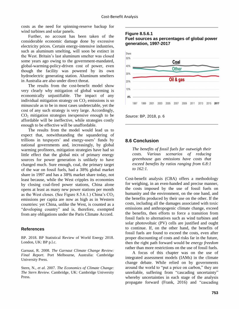
Cost-Benefit Analysis

753

costs as the need for spinning-reserve backup for

wind turbines and solar panels.

Further, no account has been taken of the

considerable economic damage done by excessive

electricity prices. Certain energy-intensive industries,

such as aluminum smelting, will soon be extinct in

the West. Britain’s last aluminum smelter was closed

some years ago owing to the government-mandated,

global-warming-policy-driven cost of power, even

though the facility was powered by its own

hydroelectric generating station. Aluminum smelters

in Australia are also under direct threat.

The results from the cost-benefit model show

very clearly why mitigation of global warming is

economically unjustifiable. The impact of any

individual mitigation strategy on CO2 emissions is so

minuscule as to be in most cases undetectable, yet the

cost of any such strategy is very large. Accordingly,

CO2 mitigation strategies inexpensive enough to be

affordable will be ineffective, while strategies costly

enough to be effective will be unaffordable.

The results from the model would lead us to

expect that, notwithstanding the squandering of

trillions in taxpayers’ and energy-users’ funds by

national governments and, increasingly, by global

warming profiteers, mitigation strategies have had so

little effect that the global mix of primary energy

sources for power generation is unlikely to have

changed much. Sure enough, coal, the primary target

of the war on fossil fuels, had a 38% global market

share in 1997 and has a 38% market share today, not

least because, while the West cripples its economies

by closing coal-fired power stations, China alone

opens at least as many new power stations per month

as the West closes. (See Figure 8.5.6.1.) China’s CO2

emissions per capita are now as high as in Western

countries: yet China, unlike the West, is counted as a

“developing country” and is, therefore, exempted

from any obligations under the Paris Climate Accord.

References

BP. 2018. BP Statistical Review of World Energy 2018.

London, UK: BP p.l.c.

Garnaut, R. 2008. The Garnaut Climate Change Review:

Final Report. Port Melbourne, Australia: Cambridge

University Press.

Stern, N., et al. 2007. The Economics of Climate Change:

The Stern Review. Cambridge, UK: Cambridge University

Press.

Figure 8.5.6.1 Fuel sources as percentages of global power generation, 1997-2017

Source: BP, 2018, p. 6

8.6 Conclusion

The benefits of fossil fuels far outweigh their

costs. Various scenarios of reducing

greenhouse gas emissions have costs that

exceed benefits by ratios ranging from 6.8:1

to 162:1.

Cost-benefit analysis (CBA) offers a methodology

for weighing, in an even-handed and precise manner,

the costs imposed by the use of fossil fuels on

humanity and the environment, on the one hand, and

the benefits produced by their use on the other. If the

costs, including all the damages associated with toxic

emissions and anthropogenic climate change, exceed

the benefits, then efforts to force a transition from

fossil fuels to alternatives such as wind turbines and

solar photovoltaic (PV) cells are justified and ought

to continue. If, on the other hand, the benefits of

fossil fuels are found to exceed the costs, even after

proper discounting of costs and risks far in the future,

then the right path forward would be energy freedom

rather than more restrictions on the use of fossil fuels.

A focus of this chapter was on the use of

integrated assessment models (IAMs) in the climate

change debate. While relied on by governments

around the world to “put a price on carbon,” they are

unreliable, suffering from “cascading uncertainty”

whereby uncertainties in each stage of the analysis

propagate forward (Frank, 2016) and “cascading

Climate Change Reconsidered II: Fossil Fuels

754

bias,” whereby high-end estimates are multiplied

together resulting in risk estimates that are orders of

magnitude greater than what empirical data suggest

(Belzer, 2012).

This chapter closely examined the IAMs used by

the IPCC and found major methodological problems

at every step. The IPCC’s emission scenarios are

little more than guesses and speculative “storylines.”

The IPCC falsely assumes the carbon cycle is

sufficiently understood and measured with sufficient

accuracy as to make possible precise predictions of

future levels of carbon dioxide (CO2) in the

atmosphere. And the IPCC relies on an estimate of

climate sensitivity – the amount of warming likely to

occur from a doubling of the concentration of

atmospheric carbon dioxide – that is out-of-date and

probably too high, resulting in inflated estimates of

future temperature change (Michaels, 2017).

The IPCC has done a masterful job compiling

research on the impacts of climate change, but it does

not distinguish between those that might be due to the

human presence and those caused by such natural

events as changes in solar radiation, volcanic activity,

or ocean currents (IPCC, 2014a, pp. 4–5). It makes

no attempt to aggregate the many studies it cites, and

since they utilize different methodologies and

definitions of terms, cover different periods of time,

and often focus on small geographic areas, such an

effort would prove impossible. The IPCC is left

saying “the impact of climate change will be small

relative to the impacts of other drivers” ” (IPCC,

2014b, p. 662), and when measured in terms of lost

gross national product (GDP), its estimate of -0.2

to -2.0% (IPCC, 2014a, p. 663) should put climate

change near the bottom of the agenda for

governments around the world.

The “social cost of carbon” (SCC) derived from

IAMs is little more than an accounting fiction created

to justify regulation of fossil fuels (Pindyck, 2013).

Model-generated numbers are without any physical

meaning, being so far removed from any empirical

data that, using the analogy provided by Risbey et al.

(1996), there are hardly any “bricks” in this edifice,

only “glue,” being the subjective judgements of the

modelers. Changing only three assumptions in two

leading IAMs – the DICE and FUND models –

reduces the SCC by an order of magnitude for the

first and changes the sign from positive to negative

for the second (Dayaratna et al., 2017). With

reasonable assumptions, IAMs show the benefits of

future climate change probably exceed its cost, even

though such models have many other assumptions

and biases that tend to exaggerate the negative effects

of greenhouse gas emissions.

The literature review conducted in earlier

chapters of this book and summarized in Figure

8.4.1.1 identified 25 impacts of fossil fuels on human

well-being. Sixteen are net benefits, only one (oil

spills) is a net cost, and the rest are either unknown or

likely to have no net impact. This finding presents a

serious challenge to any calls to restrict access to

fossil fuels. While the decisions about how to classify

each impact may be somewhat subjective, they are no

more so than those made by the IPCC when it

composed its own similar table, which appears in the

Summary for Policymakers for the Working Group II

contribution to the Fifth Assessment Report (IPCC,

2014a, pp. 21–25).

Cost-benefit analyses conducted for this chapter

and summarized in Figure 8.4.3.1 show the IPCC’s

own cost and benefit estimates put the cost of

restricting the use of fossil fuels at approximately 6.8

times greater than the benefits. Replacing the IPCC’s

unrealistically low cost estimate with ones originally

produced by Bezdek (2014, 2015) and updated for

this chapter show reducing the use of fossil fuels

costs between 32 and 48 times as much as the IPCC’s

estimate of the benefits of a slightly cooler world. If

renewable energy sources are unable to entirely

replace fossil fuels, the cost could soar to 162 times

the possible benefit. The ratio of Bezdek’s cost

estimate per ton of CO2eq and the SCC produced by

the Interagency Working Group in 2015 is 73:1 for

fossil fuel used in 2010 and 79:1 for fossil fuels used

in 2050: the cost of stopping climate change by

restricting the use of fossil fuels would be 73 to 79

times greater than the benefits, and this assumes there

are benefits.

Why is the case for fossil fuels so strong?

Because wind and solar power cannot generate

enough dispatchable energy (available 24/7) to

replace fossil fuels. Energy consumption would have

to fall to attain the IPCC’s stated goal to lower global

greenhouse emissions 40% to 70% by 2050 and to

“near zero GtCO2eq or below in 2100” (IPCC, 2014c,

pp. 10, 12). Less use of fossil fuels means slower

economic growth and lower per-capita income for

billions of people around the world, even assuming

rapidly advancing technologies and a “decoupling” of

economic growth from energy consumption.

Reducing greenhouse gas emissions to 90% below

1990 levels by 2050, the goal of the European Union,

would lower world GDP in 2050 by 24%, a loss of

some $72 trillion, the equivalent of losing eight times

the entire GDP of the United States.

Cost-Benefit Analysis

755

The major losses of per-capita income that would

be caused by achieving either the IPCC’s or the EU’s

goals for reducing greenhouse gas emissions would

be most harmful to the poor living in developed

countries and many people living in developing

countries. Recall from Chapter 3, Section 3.2.3, the

comparison of life in Ethiopia and the Netherlands,

two countries with similar natural endowments but

dramatically different in per-capita energy

consumption and per-capita incomes. People living in

Ethiopia are 10.5 times more likely to have

HIV/AIDS, 17 times more likely to die in infancy,

die 24 years sooner, and spend 99% less money on

health care (ifitweremyhome.com, n.d.).

Implementing the IPCC’s plan would slow or prevent

the arrival of life-saving energy and technologies to

millions of people living in similar conditions around

the world.

Chapter 5 described how replacing fossil fuels

with wind turbines and solar PV cells would cause

devastating damage to the environment by vastly

increasing the amount of surface area required to

grow food and generate energy. Figure 5.2.2.1

showed how using oil to produce 2,000 MW of

power requires about nine square miles, solar panels

require 129 square miles, wind turbines require 683

square miles, and ethanol an incredible 2,450 square

miles (Kiefer, 2013). Wildlife would be pushed to

extinction nearly everywhere in the world were

alternative energies relied on for most of our energy

needs.

Finally, Chapter 7 documented the close

associations between prosperity and peace, prosperity

and democracy, and democracy and peace. By

slowing economic growth around the world, a

dramatic reduction in the use of fossil fuels could

undermine some of the world’s democracies and

make wars over food and other scarce resources a

reality again. The dramatic fall in battle-related

deaths in state-based conflicts since 1946, shown in

Figure 7.1.1, could be reversed as wars broke out

around the world. Recall LeBlanc and Register

(2003, p. 229) saying the history of humanity was

“constant battles” until the prosperity, technology,

and freedom made possible by the Industrial

Revolution made peace possible. They thought “the

opportunity for humans to live in long term balance

with nature is within our grasp if we do it right.” That

vision would be lost as humanity is plunged back into

never-ending warfare by attempts to restrict access to

fossil fuels. The cost-benefit analyses conducted in this

chapter confirm that the benefits of using fossil fuels

far outweigh their costs. More than that, continued

reliance on fossil fuels is essential if we are to feed a

growing world population and still preserve space for

nature. The process that allowed humanity to

discover and put to use the tremendous energy

trapped inside fossil fuels – relying on markets to

find efficient win-win responses to climate change

and balance the interests and needs of today with

those of tomorrow – should be permitted to continue

to dictate the pace of a transition to alternatives to

fossil fuels, not irrational fears of a climate

catastrophe or hopes of technological miracles.

The global war on energy freedom, which

commenced in earnest in the 1980s and reached a

fever pitch in the second decade of the twenty-first

century, was never founded on sound science or

economics. The world’s policymakers ought to

acknowledge this truth and end that war.

References

Belzer, R. 2012. Risk assessment, safety assessment, and

the estimation of regulatory benefits. Mercatus Research.

Washington, DC: Mercatus Center.

Bezdek, R.H. 2014. The Social Costs of Carbon? No, the

Social Benefits of Carbon. Oakton, VA: Management

Information Services, Inc.

Dayaratna, K., McKitrick, R., and Kreutzer, D. 2017.

Empirically-constrained climate sensitivity and the social

cost of carbon. Climate Change Economics 8: 2.

Frank, P. 2016. Systematic error in climate measurements:

the surface air temperature record. International Seminars

on Nuclear War and Planetary Emergencies 48th Session.

Presentation in Erice, Italy on August 19–25, pp. 337–51.

Idso, C.D. 2013. The Positive Externalities of Carbon

Dioxide: Estimating the Monetary Benefits of Rising

Atmospheric CO2 Concentrations on Global Food

Production. Tempe, AZ: Center for the Study of Carbon

Dioxide and Global Change. October 21.

ifitweremyhome.com. n.d. Compare Netherlands to

Ethiopia (website). Accessed November 17, 2018.

IPCC. 2013. Intergovernmental Panel on Climate Change.

Climate Change 2013: The Physical Science Basis.

Contribution of Working Group I to the Fifth Assessment

Report of the Intergovernmental Panel on Climate Change.

Cambridge, UK: Cambridge University Press.

IPCC. 2014a. Intergovernmental Panel on Climate Change.

Summary for Policymakers. Climate Change 2014:

Impacts, Adaptation, and Vulnerability. Contribution of

Climate Change Reconsidered II: Fossil Fuels

756

Working Group II to the Fifth Assessment Report of the

Intergovernmental Panel on Climate Change. New York,

NY: Cambridge University Press.

IPCC. 2014b. Intergovernmental Panel on Climate

Change. Climate Change 2014: Impacts, Adaptation, and

Vulnerability. Part A: Global and Sectoral Aspects.

Contribution of Working Group II to the Fifth Assessment

Report of the Intergovernmental Panel on Climate Change.

New York, NY: Cambridge University Press.

IPCC. 2014c. Intergovernmental Panel on Climate Change.

Climate Change 2014: Mitigation of Climate Change.

Contribution of Working Group III to the Fifth Assessment

Report of the Intergovernmental Panel on Climate Change.

New York, NY: Cambridge University Press.

Kiefer, T.A. 2013. Energy insecurity: the false promise of

liquid biofuels. Strategic Studies Quarterly (Spring): 114–

51.

LeBlanc, S. and Register, K.E. 2003. Constant Battles:

The Myth of the Noble Savage and a Peaceful Past. New

York, NY: St. Martin’s/Griffin.

Michaels, P. 2017. Testimony. Hearing on At What Cost?

Examining the Social Cost of Carbon, before the U.S.

House of Representatives Committee on Science, Space,

and Technology, Subcommittee on Environment,

Subcommittee on Oversight. February 28.

Moore, S. and Simon, J. 2000. It’s Getting Better All the

Time: 100 Greatest Trends of the Last 100 Years.

Washington, DC: Cato Institute.

Risbey, J., Kandlikar, M., and Patwardhan, A. 1996.

Assessing integrated assessments. Climatic Change 34:

369–95.

Pindyck, R.S. 2013. Climate change policy: what do the

models tell us? Journal of Economic Literature 52 (3).