CSIS Discussion Paper No. 61

Cost-Benefit Analysis for Transport Networks

-Theory and Application- Yukihiro Kidokoro＊

Center for Spatial Information Science, University of Tokyo

Faculty of Economics, University of Tokyo, 7-3-1, Hongo, Bunkyo, Tokyo, 113-0033, Japan

Tel&Fax: +81-3-5841-5641, E-mail: kidokoro@csis.u-tokyo.ac.jp

Abstract: In this paper, practical methods for estimating benefits corresponding to the second-best

situation are derived by modeling a congestion-prone transport network explicitly. In the second-best

situation, a change in total benefit of an investment in transport infrastructure can be calculated in

three ways: (a) the sum of the changes in consumers’ and producers’ surpluses in all routes; (b) the

sum of the changes in consumers’ and producers’ surpluses in the invested routes and the change in

the deadweight loss in all other routes; and (c) the sum of a change in the total benefits in the first-best

case and a change in the deadweight loss in all routes. Applying method (c), we demonstrate that the

final benefits of distortion-relieving policies, such as introduction of congestion tolls on the

congested routes of a network, are the sum of a change in the deadweight loss in all routes.

Theoretical results are derived in practically useful forms, and then illustrated with examples that

reveal typical errors in benefit estimation for transport projects.

Keywords: cost-benefit analysis, investment in transport infrastructure, network, externality

＊ I would like to thank Richard Arnott, Ryuji Fukushima, Tatsuo Hatta, Yoshitsugu Kanemoto, Se-il Mun, Kenneth A. Small, and

Takayuki Ueda for helpful suggestions and discussions. I also thank two anonymous referees and editors for encouraging suggestions

and comments. The final version of this paper was written while I was visiting the Department of Economics, at the University of

California, Irvine. I thank the faculty members and staff there for their hospitality. Of course, I am solely responsible for any remaining

errors and omissions.

1

1 Introduction

Transport projects often require huge public funds. Thus, a cost-benefit analysis is very

important to judge if the project in question is worthy of implementing. However, it is rather difficult

to carry out cost-benefit analysis for transport projects accurately, because benefit-estimation for

transport projects has the following features, which are often less organized in the standard

textbooks1;

Transport Networks: Many transportation methods actually co-exist, and they form complex

transport networks. How do we consider transport networks in benefit-estimation for transport

projects?

Congestion: Congestion often arises in some parts of transport networks. Investments in some

parts of transport networks to relieve the congestion change the degree of congestion in all parts of

transport networks. How do we address such a congestion problem in transport networks?

Divergence between Private User Price and Social Marginal Cost: Due to political and

technical difficulties, the congestion tax is rarely adopted, and consequently, the private user price

of a trip differs from its social marginal cost in transport networks with congestion. In such a

second-best situation, how do we accurately estimate the final benefit of transport projects?

The purpose of this paper is to propose a consistent benefit-estimation method for transport

projects in a practically useful manner, including all the points stated above. Firstly, transport

networks are modeled as an economy with multiple goods, applying a general equilibrium approach,

shown in Boadway and Bruce (1984), for instance. This approach enables us to represent any kind of

transport networks, because the relationship between routes, which may be substitutes or

1 See, for example, Lesourne (1975), Sassone and Schaffer (1978), Pearce and Nash (1981), Sugden and Williams (1978), Gramlich

(1990), Layard and Glaister (1994), Brent (1996), Nas (1996), and Boardman et al. (2000).

2

complements, need not to be specified. Secondly, the degree of congestion is explicitly taken into

account in all the parts of transport networks. Thus, we can focus on the benefit-estimation in the case

where a transport project not only changes the degree of congestion in the invested area but also

changes it subsequently in all the other areas of a transport network. Thirdly, our analysis is presented

within a consistent framework from the first-best case, in which the private user prices of trips equal

their social marginal costs in all the parts of a transport network, to the second-best case, in which the

private user prices of trips differ from their social marginal costs at least in a part of a transport

network. The approach in this paper highlights how to calculate the total benefits in the second-best

case, which is less focused but practically more important than in the first-best case.

The main results of the paper are as follows. In the first-best case, the total benefits from an

investment in transport infrastructures in a route result in the sum of changes in the consumers’ and

producers’ surpluses in the invested route. In the first-best case, we do not have to consider the

accompanying changes in the other routes that have not received investment.

In the second best case, we need more elaborate calculations. The total benefits in the

second-best case can be written in three forms. The first form shows that the total benefits equal the

sum of changes in the consumers’ and producers’ surpluses in all routes. This method is a natural

extension of the benefit estimation method in the first-best case; that is, the total benefits in the

first-best case is indeed the sum of changes in the consumers’ and producers’ surpluses in all routes.

However, in the first-best case, a change in consumers’ surpluses and a change in producers’ surpluses

cancel each other out in the non-invested routes, and consequently, the total benefits to be calculated

reduces to the sum of changes in the consumers’ and producers’ surplus in the invested route only. In

the second-best case, this cancellation does not apply, and we have to calculate changes in the

consumers’ and producers’ surpluses in all routes.

The second form shows that the total benefits consist of changes in the consumers’ and

3

producers’ surpluses in the invested route and a change in the dead weight loss in all the other routes.

This second form highlights that total benefits to be calculated in non-invested routes are a change in

the dead weight loss. The second form is also related to the benefit estimation in the first-best case.

In the first-best case, no dead weight loss exists. Thus, a change in the dead weight loss are zero in all

routes, which again shows that final benefits in the first best case are the sum of changes in the

consumers’ and producers’ surplus in the invested route only.

The third form shows that the total benefits in the second-best case equal the sum of total

benefits in the first-best case and a change in the dead weight loss in all routes. The third form

highlights the relationship between the total benefits in the first-best case and those in the second-best

case, and demonstrates that their difference stems from a change in the dead weight loss in all routes.

We actually live in a second-best world, and consequently, it is often difficult to know the total

benefits under the hypothetical first-best situation. Thus, practical benefit estimation would rely on

the first and second methods. However, this does not mean that the third method is not practically

useful. The third method is not only intuitively easy to understand, but also important in conducting

benefit-estimation in the case where congestion tolls are introduced. Applying the third form in the

second-best analysis, we can easily show that the total benefits from an introduction of congestion

tolls are the sum of a change in the dead weight loss in all routes.

Before proceeding, we will briefly relate our study to the existing literature. Firstly, Kanemoto

and Mera (1985) and Jara-Diaz (1986) show that under the first-best situation with no price distortion,

a change in the benefits in transportation sectors includes all the economic benefits from a transport

project. Since we ignore the price distortion in non-transport sectors, we can also obtain final benefits

from a transport investment, by calculating changes in the benefits in the transport sector only.

However, their analysis neglects the inner structure of the transport sectors, and does not focus on the

important issues to be addressed regarding transport sectors, e.g., transport networks and congestion.

4

In this paper, we formally model transport networks with congestion and analyse the

benefit-estimation method for transport projects, explicitly considering the second-best nature in the

real world.

Secondly, benefit-estimation for actual transport networks with congestion, which are neglected

in Kanemoto and Mera (1985) and Jara-Diaz (1986), are dealt with in older literature (e.g., Harrison

(1974), Williams (1976), Jones (1977), and Jara-Diaz and Friesz (1982)). However, these analyses

are less organized or incomplete, as they do not illustrate the benefit-estimation method under the

second-best situation in detail or the relationship between the benefit-estimation in the first-best and

that in the second-best. Such deficiencies also apply to more recent literature that includes analyses

of the benefit-estimation (e.g., Button (1993), Oppenheim (1995), and Williams et al. (1991, 2001)).

Our analysis offers a practical benefit-estimation method both in the first-best case and in the

second-best case and clarifies the link between them in a consistent framework.

Thirdly, the approach in this paper is most related to Harberger (1972), Mohring (1976), and

Kanemoto (1996) in that benefit-estimation in the first-best case is explicitly distinguished from that

in the second-best case. These studies deal with the benefit estimation both in the first-best case and

in the second best case, focusing on two-parallel congestion-prone roads. However, they do not

model general transport networks and, consequently, do not fully investigate how to estimate the total

benefits from transport investments in the case of actual complex transport networks. They also do

not show that the total benefits in the second-best case can be expressed in the three forms, each of

which has practical implication. Our analysis can also be considered as a practical extension of these

studies, explicitly taking into account congestion-prone transport networks, which often have very

complex structures, especially in urban areas of large cities.

The structure of this paper is as follows. In Section 2, we set up the model. In Section 3, we

derive a benefit-estimation method for transport networks in the first-best case, in which private

5

prices of trips equal their social marginal costs in all routes. In Section 4, we focus on the second-best

case, in which private prices of trips differ from their social marginal costs, at least with respect to one

route. In Section 5, by applying our results to actual benefit estimation, we use examples to illustrate

typical errors in benefit-estimation methods for transport networks. Section 6 concludes our analysis.

2 The Model

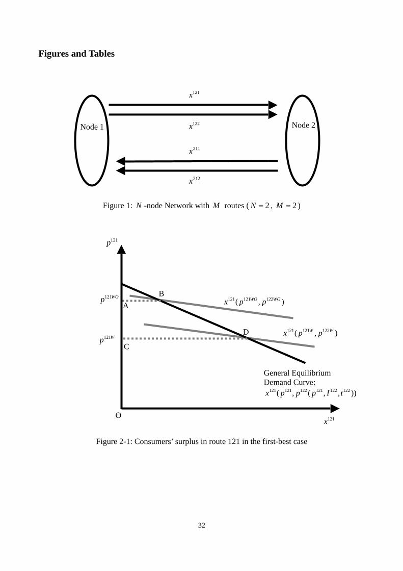
Consider a transport network in which N nodes are linked to one another. Between node i

(1 ) and node i N≤ ≤ j (1 j N≤ ≤ ), M means of transportation, which we call “routes” hereafter,

are available. One may think that M routes correspond to M kinds of transport modes or M links

in a single transport mode. The k th (1 k M≤ ≤ ) route from node i to node j is called route ijk .

The number of trips in the route ijk is denoted by ijkx . We assume that always holds. We

also assume that the number of trips from node i to node i is zero; i.e., . Figure 1 illustrates

the example of a network in which and

0ijkx >

0iikx =

2N = 2M = .

The representative consumer at node i demands the composite consumer good, , the price of

which is normalized at unity, and his or her trips from node i . Our analysis applies even if the

consumer at node i demands the trips i j or i

z

i j→ → j ′→ → ; i.e., if the consumer at node i

demands “round” trips or demands trips via another node. We assume that the utility function of the

representative consumer at node has the following quasi-linear form: i

(..., ,...)i i ijkU z u x= + , (1)

where depends on all directions of the trips from node i . The above quasi-linear utility function

implies that we neglect the income effects, and consequently, the consumers’ surplus equals the

iu

6

equivalent variation and compensating variation.2 As Willig (1976) demonstrates, the difference

between the consumers’ surplus, equivalent variation, and compensating variation is rather small, and

hence disregarding the difference is justified in benefit estimation in practice. The quasi-linear utility

function also yields the Gorman-type indirect utility function3, which justifies the summation of

individual utilities to obtain the total consumers’ surplus. In this paper, the utility function is assumed

to be concave. Note that we do not make further assumptions about the utility function. Thus, the

utility function (1) specifies no particular relationship between routes; for example, one could think

that route may be a substitute or complement for route . When 1ij 2ij M routes from node to node i

j are perfect substitutes, the utility function (1) becomes

1(...; ... ... ;...)i i ij ijk ijMU z u x x x= + + + + + , (2)

which is the utility function that is consistent with Wardrop’s (1952) analysis.

The generalized price of a trip in route , which includes time costs, is denoted by ijk ijkp . The

representative consumer at node maximizes his or her utility, (1), subject to the budget constraint: i

ijk ijk i

j k

z p x y+ =∑∑ , (3)

where is the income of the consumer at node i . We assume that the consumer does not take into

account the effect of his or her own behaviour on congestion; i.e., we assume that the consumer is a

price-taker.

iy

The maximization problem of the representative consumer at node is then formulated as: i

{ },..., ,...max (..., ,...) :

ijk

i i ijk ijk ijk i

z x j k

U z u x z p x y⎧ ⎫

= + + =⎨ ⎬⎩ ⎭

∑∑ . (4)

2 See, for example, Varian (1992).

3 See, for example, Mas-Colell et al. (1995) and Tsuneki (2000).

7

Solving the maximization problem, (4), yields

ijkijk i

xp u= , (5)

from which, we obtain the Marshallian demand function in route ijk :

(..., ,...)ijk ijk ijkx x p= . (6)

For the trips in route ijk , both investments in transport infrastructures, which are measured in

monetary terms and denoted by ijkI , and the suppliers of transport services are required. Examples of

transport infrastructures are roads, railroad trucks, and airports, and examples of the suppliers of

transport services are railway operators and airlines. In the case of road transport, one can think of the

drivers themselves as the suppliers of transport services. For the sake of exposition, we assume that

the government owns all the transport infrastructures and makes investments in them. This

assumption is innocuous for our analysis, because we do not focus on the welfare distribution but

only on the total benefits from an investment in transport infrastructures. The government imposes

“taxes,” , per trip in route ijk . This tax, , can be interpreted in many ways. In the case of road

transport, one could think of as gasoline taxes. needs not to be positive; for instance, in the

case of public transport that is subsidized by the government, one could think of as unit subsidy

per ride, which can be considered as a negative tax.

ijkt ijkt

ijkt ijkt

ijkt

Let us assume that all the suppliers of transport services in route ijk are homogenous,

sufficiently competitive with constant returns to scale, and their unit supply cost is ijkc . Since the

level of ijkc is irrelevant to our analysis, we can set it at zero. Other unit generalized costs of the trips

in route ijk , which includes monetized time costs, is , which is non-decreasing with ( , )ijk ijk ijkc x I ijkx

and decreasing with ijkI ; i.e.,

0ijk

ijkijk

ijk x

c cx∂

≡ ≥∂

(7)

8

and

0ijk

ijkijk

ijk I

c cI∂

≡ <∂

. (8)

The total cost function of the trips in route ijk , , is ijkC

( , )ijk ijk ijk ijk ijkC c x I x= , (9)

from which we can obtain their marginal cost , ijkMC , as

( , ) ( , )ijkijk ijk ijk ijk ijk ijk ijk ijk

xMC c x I c x I x= + , (10)

where shows the congestion externality that an additional trip gives to all the trips in

route ijk .

( , )ijkijk ijk ijk ijkx

c x I x

The total profits of the suppliers of transport services in route ijk , ijkπ , can be written as

( ) ( , )ijk ijk ijk ijk ijk ijk ijk ijkp t x c x I xπ = − − , (11)

where ijk ijkp t− is the net price (excluding taxes) that the suppliers receive from the consumer. As a

result of competition, the profits of each supplier of transport services become zero, which implies

that the total profits of the suppliers of transport services are also zero:

0ijkπ = . (12)

From (11) and (12), we know that the generalized price of a trip in route ijk satisfies:

( , )ijk ijk ijk ijk ijkp c x I t= + . (13)

Solving (6) and (13), we have the general equilibrium demand curve in route ijk , whose

arguments are the investments in transport infrastructure and the taxes, that is,

(..., ,...;..., ,...)ijk ijk ijk ijkx x I t= . (14)

Finally, since the profits of the suppliers of transport services are zero, the total social welfare,

, can be defined as the sum of the consumers’ utilities and the tax revenue of the government, SW

9

exclusive of investment costs, in all routes. From (9) and (13), we know that the tax revenue of the

government in route ijk can be considered as the producers’ surplus in route : ijk

ijk ijk ijk ijk ijkt x p x C= − . (15)

Thus, the total social welfare, , is SW

( ) .

i ijk ijk ijk

i i j k i j k

i ijk ijk ijk ijk

i i j k i j k

U t x I

U p x C I

= + −

= + − −

∑ ∑∑∑ ∑∑∑

∑ ∑∑∑ ∑∑∑

SW (16)

As is usual in the literature of cost-benefit analysis, we focus on the total benefits, exclusive of

investment costs. The total benefits, TB , are defined as:

( )i ijk ijk i ijk ijk ijk

i i j k i i j k

TB U t x U p x C= + = + −∑ ∑∑∑ ∑ ∑∑∑ . (17)

3 First-best Results

In this section, we obtain the results in the first-best case, in which the generalized prices of the

trips, ijkp , equal their social marginal costs, ijkMC in all routes. From (10) and (13), we know that

the first-best situation is attained when , i.e., the tax, , is set equal to the

congestion externality, in all routes.

( , )ijkijk ijk ijk ijk ijk

xt c x I x= ijkt

( , )ijkijk ijk ijk ijkx

c x I x

Suppose that an investment in transport infrastructures increases from ijkWOI to ijkWI in route

. The change in the total benefits, TB , in this case consist of: ijk

i) a change in the consumers’ surplus in route ijk :

ijkWO

ijkW

I ijkijk ijk

ijkI

dpx dIdI

⎛ ⎞⎜ ⎟⎝ ⎠

∫ (18)

and;

10

ii) a change in the tax revenue in route ijk :

ijkW

ijkWO

I ijkijk ijk

ijkI

dxtdI

⎛ ⎞⎜ ⎟⎝ ⎠

∫ dI . (19)

In sum, these two terms are reduced to:

ijkWO

ijk

ijkW

Iijk ijk ijkI

I

c x dI∫ . (20)

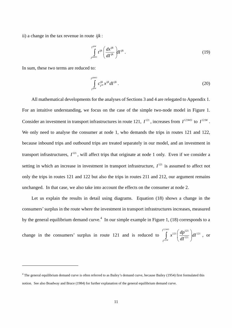
All mathematical developments for the analyses of Sections 3 and 4 are relegated to Appendix 1.

For an intuitive understanding, we focus on the case of the simple two-node model in Figure 1.

Consider an investment in transport infrastructures in route 121, 121I , increases from 121WOI to 121WI .

We only need to analyse the consumer at node 1, who demands the trips in routes 121 and 122,

because inbound trips and outbound trips are treated separately in our model, and an investment in

transport infrastructures, 121I , will affect trips that originate at node 1 only. Even if we consider a

setting in which an increase in investment in transport infrastructure, 121I is assumed to affect not

only the trips in routes 121 and 122 but also the trips in routes 211 and 212, our argument remains

unchanged. In that case, we also take into account the effects on the consumer at node 2.

Let us explain the results in detail using diagrams. Equation (18) shows a change in the

consumers’ surplus in the route where the investment in transport infrastructures increases, measured

by the general equilibrium demand curve.4 In our simple example in Figure 1, (18) corresponds to a

change in the consumers’ surplus in route 121 and is reduced to 121

121

121121 121

121

WO

W

I

I

dpx dIdI

⎛ ⎞⎜ ⎟⎝ ⎠

∫ , or

4 The general equilibrium demand curve is often referred to as Bailey’s demand curve, because Bailey (1954) first formulated this

notion. See also Boadway and Bruce (1984) for further explanation of the general equilibrium demand curve.

11

121

121

121 121

WO

W

p

p

x dp∫ where and denotes the generalized prices in route 121 corresponding to 121WOp 121Wp

121WOI and 121WI . Remember that the ordinary Marshallian demand curve is drawn on the basis that

incomes and prices in the other markets are held constant. In our model in which the utility function

is assumed to be quasi-linear, the Marshallian demand curve does not depend on income, but on

prices in the other markets. The investment in transport infrastructure in route 121, not only affects

the generalized price and demand of the trips in route 121, but also affects those of the trips in route

122, depending on the relationship between the trips in routes 121 and the trips in routes 122, which

may be substitutes or complements. Taking into account these effects, the investment in route 121

does not decrease its generalized price along its Marshallian demand curve with the generalized price

of the trips in route 122 fixed, but shifts the Marshallian demand curve. Look at Figure 2-1. With

regard to the trips in route 121, an equilibrium without a project, point B, and an equilibrium with a

project, point D, lie on different Marshallian demand curves. The general equilibrium demand curve

for the trips in route 121 is a locus of attained equilibria, which passes through points B and D, and

incorporates the accompanying change in the trips in route 122. In 121 121x p− plane in Figure 2-1, the

general equilibrium demand curve in route 121 is shown as , given 121 121 122 121 122 122( , ( , , )x p p p I t ) 122I

and . A change in the consumers’ surplus in route 121 needs to be measured along the general

equilibrium demand curve and, consequently, is . When estimating transport demand in

practice, it is often difficult to derive the Marshallian demand curve with incomes and the generalized

prices in the other trips held constant, because a change in the price of a trip increases or decreases

congestion in other trips, and subsequently, changes the generalized prices of other trips. In the actual

forecast of transport demand, accompanying changes in other trips due to substitutability and

complementarity relationships between trips are usually taken into account, at least implicitly. Thus,

122t

Area ABDC

12

the present estimation of transport demand can be regarded as a forecast of the general equilibrium

demand curve, rather than of the Marshallian demand curve.

Equation (19) shows a change in the tax revenue in the route where the investments in transport

infrastructures increase. In our example in Figure 1, (19) corresponds to 121

121

121121 121

121

W

WO

I

I

dxtdI

⎛ ⎞⎜ ⎟⎝ ⎠

∫ dI

)

. Since

ijk ijk ijk ijk ijkt x p x C= − (21)

from (15), we can consider (19) as a change in the producers’ surplus in the invested route. A change

in the producers’ surplus in route 121 can be expressed as in Figure 2-2,

which is rearranged as

- Area CDF Area ABE

(

.

Area CDF Area ABEArea CDF Area EBDC Area ABE Area EBDCArea EBDF Area ABDC

−= + − += −

(22)

It should be remembered that a change in the consumers’ surplus in route 121 is .

By adding up the changes in the consumers’ and producers’ surpluses, the change in the total benefits

in route 121 is summed up as , which is expressed as in our example

and corresponds to (20).

Area ABDC

Area EBDF121

121

121

121 121 121

WO

W

I

II

c x dI∫

In the first-best case, it is unnecessary to consider the accompanying changes in all the other

routes. To see why, let us derive the consumers’ surplus and the tax revenue in route 122.

A change in the consumers’ surplus in route 122 is derived from the understanding that the

general equilibrium demand curve in route 122 is

122122 122 122 122 122 122 122 122 122( , ) ( , )

xp MC c x I c x I x= = + (23)

in Figure 2-3. The reason is that equilibria are always on the line for (23) in 122 122x p− plane,

although an increase in the investment in transport infrastructures in route 121 shifts the Marshallian

demand curve for the trips in route 122. Thus, a change in the consumers’ surplus relating to the trip

13

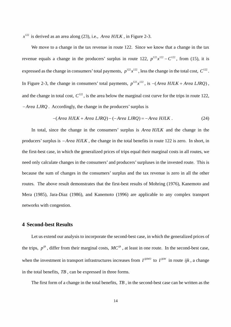
122x is derived as an area along (23), i.e., , in Figure 2-3. Area HJLK

We move to a change in the tax revenue in route 122. Since we know that a change in the tax

revenue equals a change in the producers’ surplus in route 122, 122 122 122p x C− , from (15), it is

expressed as the change in consumers’ total payments, 122 122p x , less the change in the total cost, .

In Figure 2-3, the change in consumers’ total payments,

122C

122 122p x , is ( )Area HJLK Area LJRQ− + ,

and the change in total cost, , is the area below the marginal cost curve for the trips in route 122,

. Accordingly, the change in the producers’ surplus is

122C

Area LJRQ−

( ) ( ) Area HJLK Area LJRQ Area LJRQ Area HJLK− + − − = − . (24)

In total, since the change in the consumers’ surplus is and the change in the

producers’ surplus is , the change in the total benefits in route 122 is zero. In short, in

the first-best case, in which the generalized prices of trips equal their marginal costs in all routes, we

need only calculate changes in the consumers’ and producers’ surpluses in the invested route. This is

because the sum of changes in the consumers’ surplus and the tax revenue is zero in all the other

routes. The above result demonstrates that the first-best results of Mohring (1976), Kanemoto and

Mera (1985), Jara-Diaz (1986), and Kanemoto (1996) are applicable to any complex transport

networks with congestion.

Area HJLK

Area HJLK−

4 Second-best Results

Let us extend our analysis to incorporate the second-best case, in which the generalized prices of

the trips, ijkp , differ from their marginal costs, ijkMC , at least in one route. In the second-best case,

when the investment in transport infrastructures increases from ijkWOI to ijkWI in route ijk , a change

in the total benefits, TB , can be expressed in three forms.

The first form of a change in the total benefits, , in the second-best case can be written as the TB

14

sum of:

i) a change in the consumers’ surplus in all routes:

i j k WO

i j k W

p i j ki j k ijk

ijki j k p

dpx dIdI

′ ′ ′

′ ′ ′

′ ′ ′′ ′ ′

′ ′ ′

⎛ ⎞⎜ ⎟⎝ ⎠

∑∑∑ ∫ ; (25)

and

ii) a change in the tax revenue in all routes:

ijkW

ijkWO

I i j ki j k ijk

ijki j k I

dxtdI

′ ′ ′′ ′ ′

′ ′ ′

⎛ ⎞⎜ ⎟⎝ ⎠

∑∑∑ ∫ dI , (26)

where 1 , 1i N′≤ ≤ j N′≤ ≤ , and 1 . k M′≤ ≤

The second form highlights the distinction between changes in the invested route and changes in

all the other routes, and is given by the sum of:

iii) a change in the consumers’ surplus in route ijk :

ijkWO

ijkW

I ijkijk ijk

ijkI

dpx dIdI

⎛ ⎞⎜ ⎟⎝ ⎠

∫ ; (27)

iv) a change in the tax revenue in route ijk :

ijkW

ijkWO

I ijkijk ijk

ijkI

dxtdI

⎛ ⎞⎜ ⎟⎝ ⎠

∫ dI ; (28)

and

v) a change in the dead weight loss in all the other routes:

( )ijkWO

ijkW

I i j ki j k i j k ijk

ijki j k I

dxMC p dIdI

′′ ′′ ′′′′ ′′ ′′ ′′ ′′ ′′

′′ ′′ ′′

⎛ ⎞− ⎜ ⎟

⎝ ⎠∑∑∑ ∫ , (29)

where 1 , 1i N′′≤ ≤ j N′′≤ ≤ , and 1 k M′′≤ ≤ , but ( , , )i j k′′ ′′ ′′ does not contain ( . , , )i j k

The third form highlights the distinction between the total benefits in the first-best case and the

distortions in the second-best case, and can be rearranged as the sum of:

15

vi) a change in the total benefits in the first-best case:

ijkWO

ijk

ijkW

Iijk ijk ijkI

I

c x dI∫ ; (30)

and

vii) a change in the dead weight loss in all routes:

( )ijkWO

ijkW

I i j ki j k i j k ijk

ijki j k I

dxMC p dIdI

′ ′ ′′ ′ ′ ′ ′ ′

′ ′ ′

⎛ ⎞− ⎜ ⎟

⎝ ⎠∑∑∑ ∫ . (31)

In the same way as in the first-best case in Figure 1, we explain a simple case, in which the

investment in transport infrastructure, 121I , increases from 121WOI to 121WI and affects only the trips

in routes 121 and 122.

In the first-best case, as we show in Section 3, a change in the total benefits is the sum of changes

in the consumers’ surplus and the tax revenue in route 121 and the corresponding terms in route 122.

However, with regard to the trips in route 122, the sum of changes in the consumers’ surplus and the

tax revenues is zero; consequently, the final benefits are the sum of changes in the consumers’ surplus

and the tax revenue in route 121. Even in the second-best case, the above calculation method applies

without modification; from the first form, shown in (25) and (26), we know that a change in the total

benefits is the sum of changes in the consumers’ surplus and the tax revenue in all routes.

Two different forms of a change in the total benefits in the second-best case are derived. The

second form, shown in (27)-(29), focuses on whether surpluses are generated in primary or secondary

markets.5 Firstly, we look at changes in the primary market, which corresponds to changes in the

invested route 121 in our example. A change in the consumers’ surplus is in Figure 3-1,

which is the same in the first-best case and corresponds to (27). A change in the tax revenue equals a

Area ABDC

5 This dichotomy is based on Boardman et al. (2000).

16

change in producers’ surplus from (15). Due to the discrepancy between the generalized price of a

trip and its social marginal cost, the expression of a change in producers’ surplus becomes

complicated compared to the first-best case, and is

in Figure 3-2, which

corresponds to (28). (Hereafter, in Figures 3-1, 3-2, 3-3 and 4, we omit to draw the Marshallian

demand curves to avoid unnecessary complications.)

( ) ( Area CDG O Area F D G O Area ABG O Area E B G O′′ ′ ′′ ′′ ′ ′ ′′ ′− − − )

Secondly, in the secondary market, which corresponds to the trips in route 122 in our example,

122 122 122 122 122( , )p c x I t= + (32)

always holds, regardless of shifts of the Marshallian demand curve for the trips in route 122. This

means that (32) is the general equilibrium demand curve for the trips in route 122. Accordingly, a

change in the consumers’ surplus in route 122 is in Figure 3-3, which is the same as in

the first-best case. Applying (15), a change in the tax revenues in route 122 equals a change in the

producers’ surplus,

Area HJLK

122 122 122p x C− . A change in consumers’ total payments, 122 122p x , is

in Figure 3-3, which is also the same result as in the first-best case. It

is a change in the total cost, , in the second-best case that differs from the first-best case,

reflecting the gap between the generalized price of a trip and its social marginal cost. A change in the

total cost, , in the second-best case becomes

( Area HJLK Area LJRQ− + )

122C

122C Area L J RQ′ ′− in Figure 3-3. As a result, a change

in the producers’ surplus in route 122 is

( ) ( ) Area HJLK Area LJRQ Area L J RQ Area HJLK Area L J JL′ ′ ′− + − − = − + ′ . (33)

In sum, a change in the total benefits to be calculated in the secondary market is Area L J JL′ ′ in

Figure 3-3 because changes in the consumers’ surplus, , and in (33)

cancel each other out. corresponds to (29) and shows a change in the dead weight loss

in the secondary market, which stems from a gap between the generalized price of a trip and its social

Area HJLK Area HJLK−

Area L J JL′ ′

17

marginal cost.

The third form of a change in the total benefits focuses on its relationship to the first-best result.

In route 121, a change in the consumers’ surplus is in Figure 3-1 and a change in the

producers’ surplus is ( in Figure

3-2. Superimposing Figure 3-1 on Figure 3-2 and adding up these terms, we obtain

Area ABDC

) ( )Area CDG O Area F D G O Area ABG O Area E B G O′′ ′ ′′ ′′ ′ ′ ′′ ′− − −

( ) ( ( )

Area ABDC Area CDG O Area F D G O Area ABG O Area E B G OArea ABDC Area CDG O Area ABG O Area E B G O Area F D G O

Area BDG G Area E B G O Area F D G OArea E B BDG O Area F D

′′ ′ ′′ ′′ ′ ′ ′′ ′+ − − −′′ ′ ′ ′′ ′ ′ ′′ ′′= + − + −

′′ ′ ′ ′′ ′ ′ ′′ ′′= + −′ ′′ ′′ ′ ′′ ′= −

,G O

Area E B D F Area B B B Area D D D′

′ ′ ′ ′ ′ ′′ ′ ′′= + −

)

(34)

where is a change in the total benefits in the first-best case, which corresponds to (20),

and is a change in the dead weight loss in route 121. We know that a

change in the benefits to be calculated in route 122 is a change in the dead weight loss in route 122,

which is in Figure 3-3, from the second form that focuses on the difference between the

primary market and the secondary market. In the end, we can rearrange a change in the total benefits

in the second-best case as the sum of a change in the total benefits in the first-best case, (30), and a

change in the dead weight loss in all routes, (31). The third form is an extension of Mohring’s (1976)

argument on the total benefit in the second-best case.

Area E B D F′ ′ ′ ′

Area B B B Area D D D′ ′′ ′ ′′−

Area L J JL′ ′

We have focused so far on an increase in an investment in transport infrastructures in existing

routes. However, our analysis also applies even when a new route is built, if we consider that the

investment in a new route lowers the generalized price of the trips and generates their demand. For

example, consider the building of a bridge over a river between nodes 1 and 2. Without an investment,

no bridge exists and, thus, residents cannot travel between nodes 1 and 2. With an investment,

residents can travel between nodes 1 and 2 by using the bridge. This situation can be expressed in the

following way. Without an investment, the generalized price of the trips between nodes 1 and 2 is

18

prohibitively high and, consequently, the demand for the trips between nodes 1 and 2 is zero. With an

investment, however, the generalized price of the trips between nodes 1 and 2 declines, and the

decrease in the generalized price generates the demand for the trips between nodes 1 and 2. This

interpretation implies that our analysis applies directly to newly introduced routes.

As we will show in Section 5, the first and the second forms are useful in practical

benefit-estimation. In conducting benefit estimation in practice, almost all the cases are the

second-best. Thus, it is difficult to estimate a hypothetical first-best change in the total benefits.

However, the third form, which highlights a first-best change in the total benefits and a change in the

dead weight loss in all routes, does have practical validity and is worthy to be remembered. Applying

the third form, we can easily derive a change in the total benefits when the tax increases from to

in route ijk , for example, by introducing the congestion toll. A change in the total benefits, TB ,

in this case becomes

ijkWOt

ijkWt

( )ijkWO

ijkW

t i j ki j k i j k ijk

ijki j k t

dxMC p dtdt

′ ′ ′′ ′ ′ ′ ′ ′

′ ′ ′

⎛ ⎞− ⎜ ⎟

⎝ ⎠∑∑∑ ∫ , (35)

which is the same form as (31) and shows a change in the dead weight loss in all routes.

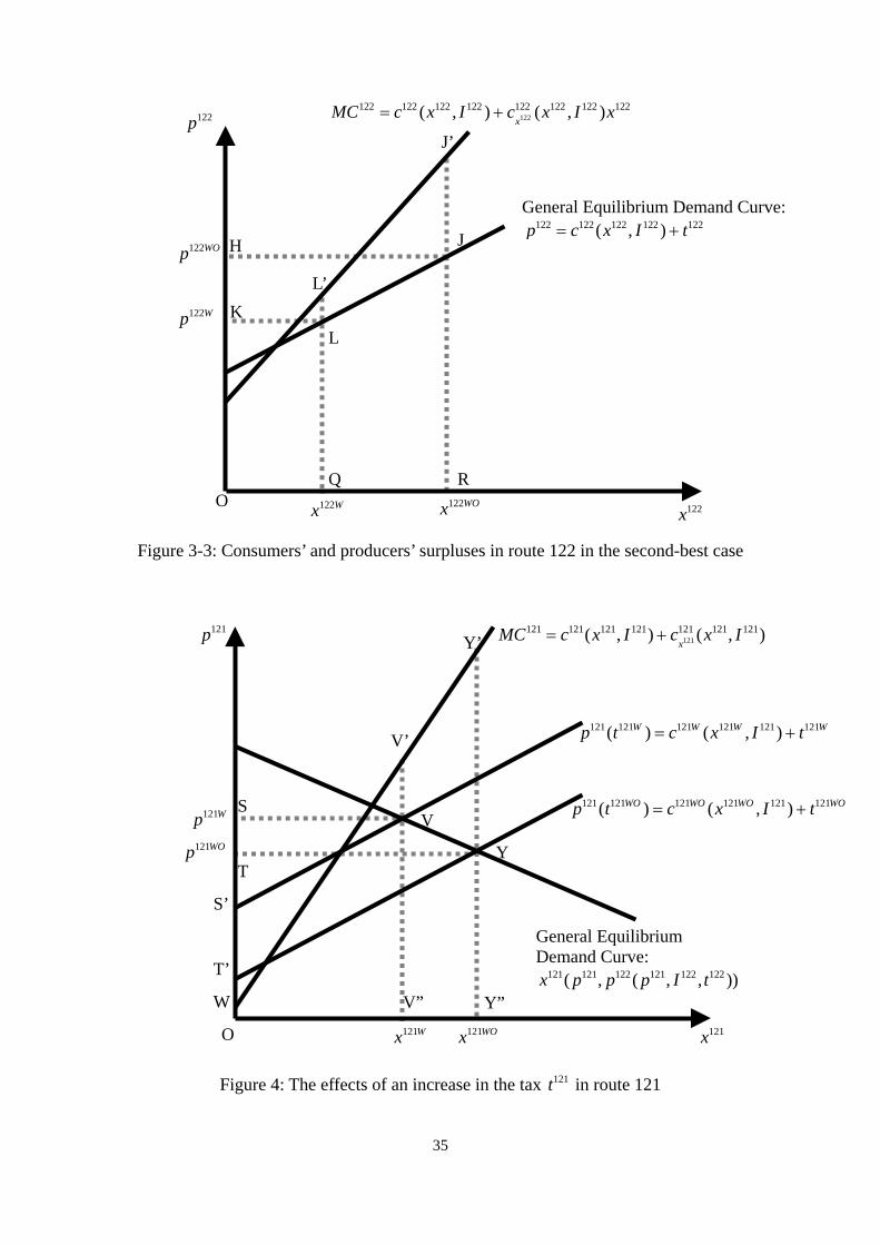
Again, we explain this on the basis of a simple example in Figure 1 and suppose that the tax in

route 121 increases. An increase in the tax in route 121 does not shift the social marginal cost curve

for the trips in route 121, unlike an increase in the investment in transport infrastructures. This

implies that in Figure 3-2, which corresponds to a change in the total benefits in the

first-best case and is expressed in (30), does not exist. In the end, the final benefits are the sum of a

change in the dead weight loss in routes 121 and 122, which corresponds to (35).

Area E B D F′ ′ ′ ′

The same result can be derived if we calculate a change in the total benefits as the sum of

changes in the consumers’ surplus and the tax revenue. In Figure 4 of route121, a change in the

consumers’ surplus is , and a change in the tax revenues, which equals the producers’ Area SVYT−

19

surplus from (15), is ( . Adding up

these terms, we obtain a change in the total benefits in route 121 of

) ( )Area SVV O Area WV V O Area TYY O Area WY Y O′′ ′ ′′ ′′ ′ ′′− − −

( ) ( ) ( ) ( ( )

,

Area SVYT Area SVV O Area WV V O Area TYY O Area WY Y OArea SVYT Area SVV O Area TYY O Area WY Y O Area WV V OArea SVYT Area SVYT Area VYY V Area V Y Y V

Area V Y YV

′′ ′ ′′ ′′ ′ ′′− + − − −′′ ′′ ′ ′′ ′ ′′= − + − + −

′′ ′′ ′ ′ ′′ ′′= − + − +′ ′=

) (36)

which is a change in the dead weight loss in route 121. In route 122, by the same argument as an

increase in an investment in transport infrastructures in the second-best case, a change in the benefits

to be calculated is a change in the dead weight loss in route 122, which is the same as Area L J JL′ ′ in

Figure 3-3. Thus, we can confirm that the final benefits are summed up as a change in the dead

weight loss in all routes.

5 Examples

Based on the analyses in Sections 3 and 4, let us check the present benefit-estimation methods,

which claim to take into account the “network characteristic” of transport. We focus on two typical

inadequacies: Examples 1 and 2 are applications of benefit estimation in the first-best and

second-best cases respectively.

Example 1: The Weighted-Average Method in the Institute for Transport Policy Studies (ITPS)

(1999)

ITPS (1999) is a manual for cost-benefit analyses of railway projects in Japan. Although ITPS

(1999) claims to take into account the effects for railways and the effects for other transport modes,

the way it estimates benefits is inconsistent with the theory developed here. We illustrate this by

using a numerical example from pp. 104–124 of ITPS (1999). The data used to calculate benefits are

given in Table 1, from which we know that this railway project shortens rail travel time and increases

20

rail demand.

In this example, it is assumed that the time cost does not depend on the volume of demand (i.e.,

no congestion exists) and no tax exists. Since the tax and the congestion externality equal zero, we

can apply the benefit-estimation method in the first-best case. Thus, a change in the total benefits is

derived as the sum of a change in the consumers’ surplus and a change in the tax revenues in the

invested route, i.e., rail. In this example, given the assumption of no tax, a change in the total benefits

is simply a change in the consumers’ surplus relating to rail. We assume that time costs are 39.3

yen/minute, as in ITPS (1999), and that the general equilibrium demand curve is linearly

approximated. Rail’s generalized price without a project is

39.3 190 11,000 18,467× + = (yen). (37)

The corresponding price with a project is

39.3 140 11,000 16,502× + = (yen). (38)

Hence, the final benefits are

0.5 (18,467-16,502) (100 135) 230,888× × + = (yen). (39)

In contrast, the benefit-estimation method in ITPS (1999) is as follows. First, we obtain the

origin-destination (OD) generalized price, which is the demand-weighted average of generalized

prices in all routes. The OD generalized price without a project is

100 110 10(39.3 190 11,000) (39.3 120 14,000) (39.3 400 5,500)220 220 220

18,717 (yen)

× + × + × + × + × + ×

= (40)

The corresponding price with a project is

135 80 5(39.3 140 11,000) (39.3 120 14,000) (39.3 400 5,500)220 220 220

17,414 (yen)

× + × + × + × + × + ×

= (41)

Second, this change in the OD generalized price is assumed to apply to all the demand in the OD.

21

Thus, the final benefits are

0.5 (18,717-17,414) (220+220) 286,660 (yen)× × = .6 (42)

Hence, the benefit-estimation method in ITPS (1999) overestimates true benefits by about 24 per

cent.

In general, the benefit-estimation method in ITPS (1999) is unreliable. However, if all

routes—rail, air, and car in this example—are assumed to be perfect substitutes, i.e., the utility

function is assumed to be like (2), the ITPS (1999) method happens to give the right value. This is

because the generalized prices of the trips between nodes i and are equal in all routes actually used

in such a case and, consequently, the generalized price in each route is equal to the demand-weighted

average of the generalized prices in all routes. However, it is not necessary to calculate the

demand-weighted average of the generalized prices in such a case when the generalized prices of the

trips are equal in all routes. Thus, even in this case, we can conclude that the ITPS (1999) method

lacks practical validity.

j

It is sometimes suggested that the ITPS (1999) method, which uses the OD generalized price, is

consistent with the estimation of transport demand using the logit model.7 However, this is incorrect.

If a discrete choice model such as the logit model is used to estimate transport demand, the general

method of estimating welfare changes in discrete choice models developed by Williams (1977) and

Small and Rosen (1981) must be used to calculate welfare changes. As Anderson et al. (1992) show,

the logit model can be interpreted as a special case of the ordinary utility-maximization problem of a

representative consumer. Thus, the methods derived in Sections 3 and 4 are still valid with

logit-based estimation of transport demand. That is, we can accurately calculate a change in the total

6 Although the total benefit is given as 326,260 (yen) in ITPS (1999), this figure is the result of a simple error in calculation.

7 See, for example, Ueda et al. (2002).

22

benefits by using the methods in Sections 3 and 4, whether or not the logit model is used to estimate

transport demand8. The ITPS (1999) OD-based method is theoretically inconsistent with both the

method developed by Williams (1977) and Small and Rosen (1981) and the method derived in this

paper; therefore, it cannot correctly compute welfare changes even when the estimation of transport

demand is logit-based.

Example 2: “Network effects” in Button (1993)

Button (1993, pp. 182–184) proposes a benefit-estimation method for transportation projects

that takes into account “network effects.” He claims that a change in the total benefits from an

investment in a route in the road network is the sum of a change in the consumers’ surplus in all routes.

However, this argument is inadequate, because it ignores a change in tax revenue. In the first-best

case, this omission obviously could be very significant; the true benefits are the sum of changes in

consumers’ surplus and the tax revenue in the invested route, not the sum of changes in consumers’

surplus in all routes. In the second-best case, the omission of the tax revenues would be justified if the

tax was regarded as zero. However, as Button himself suggests (e.g., Table 4.10 in p. 81), the

revenues from road tax (e.g., fuel tax) are too large to ignore. If we assume that a change in the tax

revenue is zero when it is actually quite large, the final benefits could be quite different from those

calculated by Button’s method.

Let us check how the omission of the producers’ surplus affects the results, using an illustrative

example, in which rail and car are available. To simplify the calculation, the time cost is assumed to

be 40 (yen/minute). Consider a transport project that upgrades rail tracks to shorten rail travel time.

Consequently, the project increases rail demand and reduces car demand. A decrease in car demand

8 See Kidokoro (2003) for a detailed analysis.

23

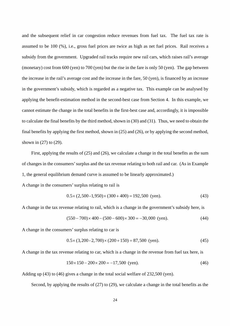
and the subsequent relief in car congestion reduce revenues from fuel tax. The fuel tax rate is

assumed to be 100 (%), i.e., gross fuel prices are twice as high as net fuel prices. Rail receives a

subsidy from the government. Upgraded rail tracks require new rail cars, which raises rail’s average

(monetary) cost from 600 (yen) to 700 (yen) but the rise in the fare is only 50 (yen). The gap between

the increase in the rail’s average cost and the increase in the fare, 50 (yen), is financed by an increase

in the government’s subsidy, which is regarded as a negative tax. This example can be analysed by

applying the benefit-estimation method in the second-best case from Section 4. In this example, we

cannot estimate the change in the total benefits in the first-best case and, accordingly, it is impossible

to calculate the final benefits by the third method, shown in (30) and (31). Thus, we need to obtain the

final benefits by applying the first method, shown in (25) and (26), or by applying the second method,

shown in (27) to (29).

First, applying the results of (25) and (26), we calculate a change in the total benefits as the sum

of changes in the consumers’ surplus and the tax revenue relating to both rail and car. (As in Example

1, the general equilibrium demand curve is assumed to be linearly approximated.)

A change in the consumers’ surplus relating to rail is

0.5 (2,500 -1,950) (300 400) 192,500× × + = (yen). (43)

A change in the tax revenue relating to rail, which is a change in the government’s subsidy here, is

(550 700) 400 (500 600) 300 30,000− × − − × = − (yen). (44)

A change in the consumers’ surplus relating to car is

0.5 (3,200 - 2,700) (200 150) 87,500× × + = (yen). (45)

A change in the tax revenue relating to car, which is a change in the revenue from fuel tax here, is

150 150 200 200 17,500× − × = − (yen). (46)

Adding up (43) to (46) gives a change in the total social welfare of 232,500 (yen).

Second, by applying the results of (27) to (29), we calculate a change in the total benefits as the

24

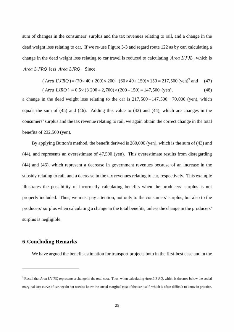
sum of changes in the consumers’ surplus and the tax revenues relating to rail, and a change in the

dead weight loss relating to car. If we re-use Figure 3-3 and regard route 122 as by car, calculating a

change in the dead weight loss relating to car travel is reduced to calculating , which is

less . Since

Area L J JL′ ′

Area L J RQ′ ′ Area LJRQ

( ) Area L J RQ′ ′ (70 40 200) 200 (60 40 150) 150 217,500= × + × − × + × = (yen)9 and (47)

( ) Area LJRQ 0.5 (3,200 2,700) (200 150) 147,500= × + × − = (yen), (48)

a change in the dead weight loss relating to the car is 217,500 147,500 70,000− = (yen), which

equals the sum of (45) and (46). Adding this value to (43) and (44), which are changes in the

consumers’ surplus and the tax revenue relating to rail, we again obtain the correct change in the total

benefits of 232,500 (yen).

By applying Button’s method, the benefit derived is 280,000 (yen), which is the sum of (43) and

(44), and represents an overestimate of 47,500 (yen). This overestimate results from disregarding

(44) and (46), which represent a decrease in government revenues because of an increase in the

subsidy relating to rail, and a decrease in the tax revenues relating to car, respectively. This example

illustrates the possibility of incorrectly calculating benefits when the producers’ surplus is not

properly included. Thus, we must pay attention, not only to the consumers’ surplus, but also to the

producers’ surplus when calculating a change in the total benefits, unless the change in the producers’

surplus is negligible.

6 Concluding Remarks

We have argued the benefit-estimation for transport projects both in the first-best case and in the

9 Recall that Area L’J’RQ represents a change in the total cost. Thus, when calculating Area L’J’RQ, which is the area below the social

marginal cost curve of car, we do not need to know the social marginal cost of the car itself, which is often difficult to know in practice.

25

second best case, explicitly modeling congestion-prone transport networks. In a practical

benefit-estimation for transport projects, the second-best situations are common, although they have

not been analysed systematically in the literature. Our main results are summed up as follows. In the

second-best situation, a change in the total benefits from an investment in transport infrastructures

can be calculated in three ways. The first method shows that a change in total benefits is the sum of

changes in consumers’ and producers’ surpluses in all routes. In all the non-invested routes, the sum

of changes in consumers’ and producers’ surpluses result in a change in the dead weight loss, caused

by the discrepancy between the generalized prices of trips and their social marginal costs. Focusing

on this feature, the second method shows that a change in the total benefits is the sum of changes in

the consumers’ and producers’ surpluses in the invested route and a change in the dead weight loss in

all the other routes. The third method shows that a change in the total benefits in the second-best case

equals the sum of a change in the total benefits in the first-best case and a change in the dead weight

loss in all routes, highlighting the relationship between the total benefits in the first-best case and

those in the second-best case. Although the first and the second methods are easy to implement

practically, the implications of the third method is very important. Applying the third method, we

know that a change in the total benefits is a change in the dead weight loss in all routes only, if the

social marginal cost curve does not shift and consequently, a change in the total benefits in the first

best case is zero. For example, when the congestion tax is introduced, a change in the total benefits

can be calculated as a change in the dead weight loss in all routes.

In concluding the paper, we comment on two issues. Firstly, in our model, the dead weight loss

arises because the generalized prices of trips differ from their social marginal costs due to the gap

between the tax, , and the congestion externality, . Our analysis also applies

without modification when the dead weight loss stems from other distortions. As an example,

consider the case in which suppliers of transport services behave less competitively. Even in this case,

ijkt ( , )ijkijk ijk ijk ijkx

c x I x

26

our analysis is directly applicable, if the tax, , is redefined to include the price-cost margin that

results from imperfect competition. Our analysis also applies to the case where the generalized prices

differs from the social marginal costs due to environmental externality, if environmental costs are

additionally included in the total cost function of trips.

ijkt

Secondly, we have assumed away the price-cost divergences in non-transport sectors. Although

it would be difficult to include them in practical benefit estimation of transport projects, our analysis

is applicable in principle, even if we explicitly consider the second-best situation in non-transport

sectors. In that case, all we have to do is to add changes in consumers’ and producers’ surpluses in

non-transport sectors. Since the same logic as changes in the non-invested routes applies to changes

in non-transport sectors, the sum of changes in consumers’ and producers’ surpluses in a

non-transport sectors equals a change in the dead weight loss in the non-transport sectors. Thus, we

can add a change in the dead weight loss in all non-transport sectors, instead of the sum of changes in

consumers’ and producers’ surpluses.

27

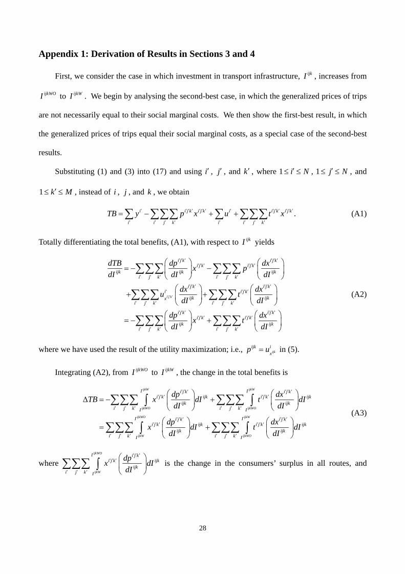
Appendix 1: Derivation of Results in Sections 3 and 4

First, we consider the case in which investment in transport infrastructure, ijkI , increases from

ijkWOI to ijkWI . We begin by analysing the second-best case, in which the generalized prices of trips

are not necessarily equal to their social marginal costs. We then show the first-best result, in which

the generalized prices of trips equal their social marginal costs, as a special case of the second-best

results.

Substituting (1) and (3) into (17) and using i′ , j′ , and k ′ , where 1 i N′≤ ≤ , 1 , and

, instead of , , and , we obtain

j N′≤ ≤

1 k M′≤ ≤ i j k

.i i j k i j k i i j k i j k

i i j k i i j k

TB y p x u t x′ ′ ′ ′ ′ ′ ′ ′ ′ ′ ′ ′ ′ ′

′ ′ ′ ′ ′ ′ ′ ′

= − + +∑ ∑∑∑ ∑ ∑∑∑ (A1)

Totally differentiating the total benefits, (A1), with respect to ijkI yields

i j k

i j k i j ki j k i j k

ijk ijk ijki j k i j k

i j k i j ki i j k

ijk ijkxi j k i j k

i j ki j k i j

ijki j k

dTB dp dxx pdI dI dI

dx dxu tdI dI

dp x tdI

′ ′ ′

′ ′ ′ ′ ′ ′′ ′ ′ ′ ′ ′

′ ′ ′ ′ ′ ′

′ ′ ′ ′ ′ ′′ ′ ′ ′

′ ′ ′ ′ ′ ′

′ ′ ′′ ′ ′ ′ ′ ′

′ ′ ′

⎛ ⎞ ⎛= − −⎜ ⎟ ⎜

⎝ ⎠ ⎝⎛ ⎞ ⎛ ⎞

+ +⎜ ⎟ ⎜ ⎟⎝ ⎠ ⎝ ⎠

⎛ ⎞= − +⎜ ⎟

⎝ ⎠

∑∑∑ ∑∑∑

∑∑∑ ∑∑∑

∑∑∑

⎞⎟⎠

i j kk

ijki j k

dxdI

′ ′ ′

′ ′ ′

⎛ ⎞⎜ ⎟⎝ ⎠

∑∑∑

(A2)

where we have used the result of the utility maximization; i.e., ijkijk i

xp u= in (5).

Integrating (A2), from ijkWOI to ijkWI , the change in the total benefits is

ijkW ijkW

ijkWO ijkWO

ijkWO

ijkW ijkW

I Ii j k i j ki j k ijk i j k ijk

ijk ijki j k i j kI I

I i j k i j ki j k ijk i j k ijk

ijk ijki j k I I

dp dxTB x dI t dIdI dI

dp dxx dI t dIdI dI

′ ′ ′ ′ ′ ′′ ′ ′ ′ ′ ′

′ ′ ′ ′ ′ ′

′ ′ ′ ′ ′ ′′ ′ ′ ′ ′ ′

′ ′ ′

⎛ ⎞ ⎛ ⎞∆ = − +⎜ ⎟ ⎜ ⎟

⎝ ⎠ ⎝ ⎠

⎛ ⎞ ⎛ ⎞= +⎜ ⎟ ⎜ ⎟

⎝ ⎠ ⎝ ⎠

∑∑∑ ∑∑∑∫ ∫

∑∑∑ ∫ijkW

O

I

i j k′ ′ ′∑∑∑ ∫

(A3)

where ijkWO

ijkW

I i j ki j k ijk

ijki j k I

dpx dIdI

′ ′ ′′ ′ ′

′ ′ ′

⎛ ⎞⎜ ⎟⎝ ⎠

∑∑∑ ∫ is the change in the consumers’ surplus in all routes, and

28

ijkW

ijkWO

I i j ki j k ijk

ijki j k I

dxtdI

′ ′ ′′ ′ ′

′ ′ ′

⎛ ⎞⎜ ⎟⎝ ⎠

∑∑∑ ∫ dI is the change in the tax revenue in all routes.

Distinguishing changes in the primary market, which is the invested-in route, from those in the

secondary market, which incorporates all other routes, using (10) and (13), we rearrange (A3) to

obtain the second form as follows:

ijkWO ijkW

ijkW ijkWO

ijkWO ijkWO

ijkW ijkW

I Ii j k i j ki j k ijk i j k ijk

ijk ijki j k i j kI I

I Iijk i j kijk ijk i j k ijk

ijk ijkkI I

dp dxTB x dI t dIdI dI

dp dpx dI x dIdI dI

′ ′ ′ ′ ′ ′′ ′ ′ ′ ′ ′

′ ′ ′ ′ ′ ′

′′ ′′ ′′′′ ′′ ′′

′′

⎛ ⎞ ⎛ ⎞∆ = +⎜ ⎟ ⎜ ⎟

⎝ ⎠ ⎝ ⎠

⎛ ⎞ ⎛ ⎞= +⎜ ⎟ ⎜ ⎟

⎝ ⎠ ⎝ ⎠

∑∑∑ ∑∑∑∫ ∫

∫ ∫ijkW ijkW

ijkWO ijkWO

ijkWO ijkW

i j k

ijkW ijkWO

i j

I Iijk i j kijk ijk i j k ijk

ijk ijki j kI I

I Iijk ijkijk ijk ijk ijk i

ijk ijk xI I

dx dxt dI t dIdI dI

dp dxx dI t dI cdI dI

′′ ′′ ′′

′′ ′′

′′ ′′ ′′′′ ′′ ′′

′′ ′′ ′′

′′

⎛ ⎞ ⎛ ⎞+ +⎜ ⎟ ⎜ ⎟

⎝ ⎠ ⎝ ⎠

⎛ ⎞ ⎛ ⎞= + +⎜ ⎟ ⎜ ⎟

⎝ ⎠ ⎝ ⎠

∑∑∑

∑∑∑∫ ∫

∫ ∫ ( )

( )

ijkWO

ijkW

ijkWO ijkW

ijkW ijkWO

I i j kj k i j k i j k ijk

ijki j k I

I Iijk ijk i j kijk ijk ijk ijk i j k i j k

ijk ijk ijkI I I

dxx t ddI

dp dx dxx dI t dI MC pdI dI dI

′′ ′′ ′′′′ ′′ ′′ ′′ ′′ ′′ ′′ ′′

′′ ′′ ′′

′′ ′′ ′′′′ ′′ ′′ ′′ ′′ ′′

⎛ ⎞− ⎜ ⎟

⎝ ⎠

⎛ ⎞ ⎛ ⎞ ⎛ ⎞= + + −⎜ ⎟ ⎜ ⎟ ⎜ ⎟

⎝ ⎠ ⎝ ⎠ ⎝ ⎠

∑∑∑ ∫

∫ ∫ijkWO

ijkW

Iijk

i j k

dI′′ ′′ ′′∑∑∑ ∫

I

(A4)

where 1 , 1 , and 1i N′′≤ ≤ j N′′≤ ≤ k M′′≤ ≤ , but ( , , )i j k′′ ′′ ′′ does not contain ( . In (A4), , , )i j k

ijkWO

ijkW

I ijkijk ijk

ijkI

dpx dIdI

⎛ ⎞⎜ ⎟⎝ ⎠

∫ is the change in the consumers’ surplus in route ijk , ijkW

ijkWO

I ijkijk ijk

ijkI

dxtdI

⎛ ⎞⎜ ⎟⎝ ⎠

∫ dI is the

change in the tax revenue in route ijk , and ( )ijkWO

ijkW

I i j ki j k i j k ijk

ijki j k I

dxMC p dIdI

′′ ′′ ′′′′ ′′ ′′ ′′

′′ ′′ ′′

⎛ ⎞− ⎜ ⎟

⎝ ⎠∑∑∑ ∫ ′′ ′′ is the change

in the deadweight loss in all other routes.

Highlighting the distinction between total benefits in the first-best case and distortions in the

second-best case, using (10) and (13) to rearrange (A3), we obtain the third form as follows:

29

ijkWO ijkW

ijkW ijkWO

ijkWO

ijk ijk i j k

ijkW

I Ii j k i j ki j k ijk i j k ijk

ijk ijki j k i j kI I

I ijkijk ijk ijk ijk i j k i j

ijkI x xI

dp dxTB x dI t dIdI dI

dxx c c dI x cdI

′′ ′′ ′′

′ ′ ′ ′ ′ ′′ ′ ′ ′ ′ ′

′ ′ ′ ′ ′ ′

′′ ′′ ′′ ′′ ′′ ′′

⎛ ⎞ ⎛ ⎞∆ = +⎜ ⎟ ⎜ ⎟

⎝ ⎠ ⎝ ⎠

⎡ ⎤⎛ ⎞= + +⎢ ⎥⎜ ⎟

⎝ ⎠⎣ ⎦

∑∑∑ ∑∑∑∫ ∫

∫

( )

ijkWO ijkWO

ijkW ijkW

ijkWO ijkW

ijk i j k

ijkW ijkW

I Ii j k i j kk ijk i j k ijk

ijk ijki j k i j kI I

I I i j kijk ijk ijk i j k i j k i j k

ijkI xI I

dx dxdI t dIdI dI

dxc x dI c x tdI

′ ′ ′

′′ ′′ ′′ ′ ′ ′′ ′ ′

′′ ′′ ′′ ′ ′ ′

′ ′ ′′ ′ ′ ′ ′ ′ ′ ′ ′

⎡ ⎤⎛ ⎞ ⎛ ⎞−⎢ ⎥⎜ ⎟ ⎜ ⎟

⎝ ⎠ ⎝ ⎠⎣ ⎦

⎛ ⎞= + − ⎜ ⎟

⎝ ⎠

∑∑∑ ∑∑∑∫ ∫

∫

( ) .

O

ijkWO ijkWO

ijk

ijkW ijkW

ijk

i j k

I I i j kijk ijk ijk i j k i j k ijk

ijkIi j kI I

dI

dxc x dI MC p dIdI

′ ′ ′

′ ′ ′′ ′ ′ ′ ′ ′

′ ′ ′

⎛ ⎞= + − ⎜ ⎟

⎝ ⎠

∑∑∑ ∫

∑∑∑∫ ∫ (A5)

In (A5), is the change in the total benefits in the first-best case, which is derived

subsequently, and

ijkWO

ijk

ijkW

Iijk ijk ijkI

I

c x dI∫

( )ijkWO

ijkW

I i j ki j k i j k ijk

ijki j k I

dxMC p dIdI

′ ′ ′′ ′ ′ ′ ′ ′

′ ′ ′

⎛ ⎞− ⎜ ⎟

⎝ ⎠∑∑∑ ∫ is the change in the deadweight loss

relating to all routes.

In the first-best case, in which the generalized prices of the trips equal their social marginal costs

in all routes, from (A4) and (A5), we obtain

ijkWO ijkW ijkWO

ijk

ijkW ijkWO ijkW

I I Iijk ijkijk ijk ijk ijk ijk ijk ijk

ijk ijk II I I

dp dxSW x dI t dI c x dIdI dI

⎛ ⎞ ⎛ ⎞∆ = + =⎜ ⎟ ⎜ ⎟

⎝ ⎠ ⎝ ⎠∫ ∫ ∫ . (A6)

Equation (A6) shows that a change in total benefits in the first-best case consists of a change in the

consumers’ surplus in route ijk , ijkWO

ijkW

I ijkijk ijk

ijkI

dpx dIdI

⎛ ⎞⎜ ⎟⎝ ⎠

∫ , and a change in the tax revenue in route ijk ,

ijkW

ijkWO

I ijkijk ijk

ijkI

dxtdI

⎛ ⎞⎜ ⎟⎝ ⎠

∫ dII

I

c x∫, and that these two terms are reduced to . Thus,

corresponds to the change in total benefits in the first-best case.

ijkWO

ijk

ijkW

Iijk ijk ijkI

I

c x dI∫ijkWO

ijk

ijkW

Iijk ijk ijkdI

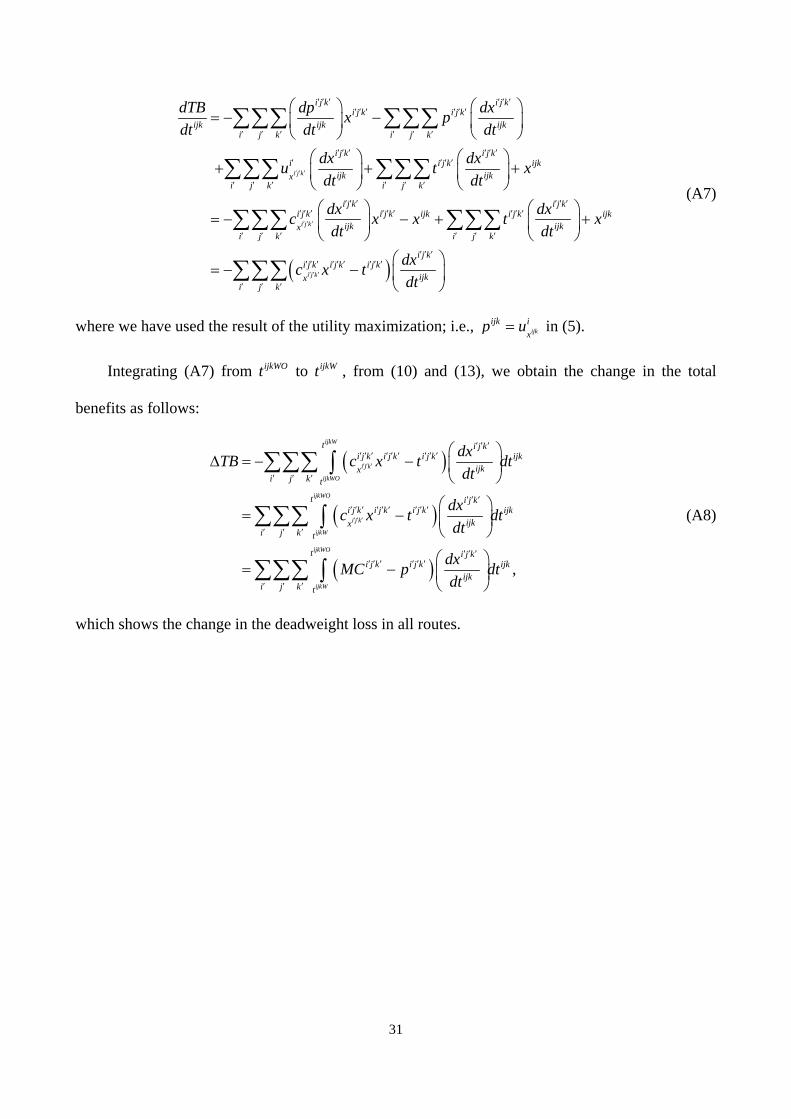
Second, let us focus on the case in which the tax in route ijk , , increases from to .

Totally differentiating total benefits, (A1) with respect to yields

ijkt ijkWOt ijkWt

ijkt

30

i j k

i j k

i j k i j ki j k i j k

ijk ijk ijki j k i j k

i j k i j ki i j k ijk

ijk ijkxi j k i j k

i j ki j k i

ijkx

dTB dp dxx pdt dt dt

dx dxu t xdt dt

dxc xdt

′ ′ ′

′ ′ ′

′ ′ ′ ′ ′ ′′ ′ ′ ′ ′ ′

′ ′ ′ ′ ′ ′

′ ′ ′ ′ ′ ′′ ′ ′ ′

′ ′ ′ ′ ′ ′

′ ′ ′′ ′ ′ ′ ′

⎛ ⎞ ⎛ ⎞= − −⎜ ⎟ ⎜ ⎟

⎝ ⎠ ⎝ ⎠⎛ ⎞ ⎛ ⎞

+ + +⎜ ⎟ ⎜ ⎟⎝ ⎠ ⎝ ⎠⎛ ⎞

= − ⎜ ⎟⎝ ⎠

∑∑∑ ∑∑∑

∑∑∑ ∑∑∑

( )i j k

i j kj k ijk i j k ijk

ijki j k i j k

i j ki j k i j k i j k

ijkxi j k

dxx t xdt

dxc x tdt

′ ′ ′

′ ′ ′′ ′ ′ ′

′ ′ ′ ′ ′ ′

′ ′ ′′ ′ ′ ′ ′ ′ ′ ′ ′

′ ′ ′

⎛ ⎞− + +⎜ ⎟

⎝ ⎠⎛ ⎞

= − − ⎜ ⎟⎝ ⎠

∑∑∑ ∑∑∑

∑∑∑

(A7)

where we have used the result of the utility maximization; i.e., ijkijk i

xp u= in (5).

Integrating (A7) from to , from (10) and (13), we obtain the change in the total

benefits as follows:

ijkWOt ijkWt

( )

( )

( )

ijkW

i j k

ijkWO

ijkWO

i j k

ijkW

ijkW

ijkW

t i j ki j k i j k i j k ijk

ijkxi j k t

t i j ki j k i j k i j k ijk

ijkxi j k t

t i j ki j k i j k

ijkt

dxTB c x t dtdt

dxc x t dtdt

dxMC pdt

′ ′ ′

′ ′ ′

′ ′ ′′ ′ ′ ′ ′ ′ ′ ′ ′

′ ′ ′

′ ′ ′′ ′ ′ ′ ′ ′ ′ ′ ′

′ ′ ′

′ ′ ′′ ′ ′ ′ ′ ′

⎛ ⎞∆ = − − ⎜ ⎟

⎝ ⎠

⎛ ⎞= − ⎜ ⎟

⎝ ⎠

⎛ ⎞= − ⎜ ⎟

⎝ ⎠

∑∑∑ ∫

∑∑∑ ∫

,O

ijk

i j k

dt′ ′ ′∑∑∑ ∫

(A8)

which shows the change in the deadweight loss in all routes.

31

Figures and Tables

Node 2Node 1

212x

211x

122x

121x

Figure 1: -node Network with N M routes ( 2N = , 2M = ) 121x

121 121 122( ,WO WOx p p )

)121 121 122( ,W Wx p p

General Equilibrium Demand Curve:

121 121 122 121 122 122( , ( , , )x p p p I t

O

121p

D

B A

C

121WOp

121Wp

)

Figure 2-1: Consumers’ surplus in route 121 in the first-best case

32

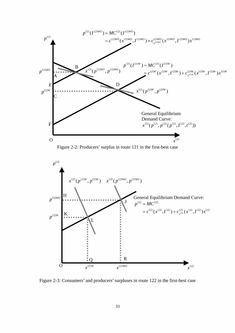
Figure 2-2: Producers’ surplus in route 121 in the first-best

O

121p

A

B

D

C

E

121 121 122( ,WO WOx p p )

)

121

121 121 121 121

121 121 121 121 121 121 121

( ) ( )( , ) ( , )WO

WO WO

WO WO WO WO WO WO WOx

p I MC Ic x I c x I x

=

= +

121

121 121 121 121

121 121 121 121 121 121 121

( ) ( )( , ) ( , )W

W W

W W W W W W Wx

p I MC Ic x I c x I x

=

= +

121 121 122 121 122 122( , ( , , ))x p p p I t

General Equilibrium Demand Curve:

121 121 122( ,W Wx p p121Wp

121WOp

F

121x

Q 122WOx122Wx

RO

122p

H

L

J General Equilibrium

122 122

122 122 122( ,p MC

c x I=

=

122 122 121( ,WO WOx p p) )122 122 121( ,W Wx p p

K

122WOp

122Wp

Figure 2-3: Consumers’ and producers’ surpluses in route 122 in the

33

case

122x

Demand Curve:

122

122 122 122 122) ( , )x

c x I x+

first-best case

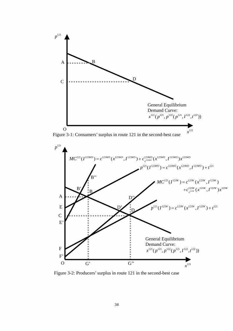
Figure 3-1: Consumers’ surplus in route 121 in the second-best case O 121x

121p

General Equilibrium Demand Curve:

121 121 122 121 122 122( , ( , , )x p p p I t )

D

B A

C

G’ G’’O 121x

121p

A B

D C

E

F

121 121 121 121 121 121( ) ( , )WO WO WO WOp I c x I t= +

121 121 121 121 121 121( ) ( , )W W W Wp I c x I= + t

121121 121 121 121 121 121 121 121 121( ) ( , ) ( , )WO

WO WO WO WO WO WO WO WOx

MC I c x I c x I x= +

General Equilibrium Demand Curve:

121 121 122 121 122 122( , ( , , ))x p p p I t

B’’

B’

F’

E’

D’

D’’121

121 121 121 121 121

121 121 121 121

( ) ( , )( , )W

W W W W

W W W Wx

MC I c x Ic x I x

=

+

Figure 3-2: Producers’ surplus in route 121 in the second-best case

34

122WOx122Wx

Q

122p

H

L

J

K

R

122122 122 122 122 122 122 122 122( , ) ( , )

xMC c x I c x I x= +

General Equilibrium Demand Curve: 122 122 122 122 122( , )p c x I t= +

122WOp

122Wp

L’

J’

122x

Figure 3-3: Consumers

O

121p

S

T

W

121WOp

121Wp

T’

S’

Figure 4: T

O

’ and producers’ surpluses in route 122 in the second

121Wx

V

Y

121 121( )WOp t =

121 121( )Wp t =

121 121 121 121( , )MC c x I= +

Y” 121WOx

121 121 122 121( , (x p p p

General EquilibriuDemand Curve:

V”

Y’

V’

he effects of an increase in the tax in route 121121t

35

-best case

121x

121 121 121 121( , )WO WO WOc x I t+

121 121 121 121( , )W W Wc x I t+

121121 121 121( ,x

)c x I

122 122, , ))I t

m

Table 1: An example from ITPS (1999)

Without a Project

Mode Travelling time

(minutes)

Monetary price (yen)

Demand per day

Rail 190 11,000 100 Air 120 14,000 110 Car 400 5,500 10

With a Project

Mode Travelling time

(minutes)

Monetary price (yen)

Demand per day

Rail 140 11,000 135 Air 120 14,000 80 Car 400 5,500 5

Table 2: An example in which the producers’ surplus plays an important role

Without a Project

Mode Travelling time

(minutes) Monetary price (yen)

Net fuel price (yen)

Fuel tax (yen)

Rail’s average

cost (yen)Generalized price (yen)

Demand per day

Rail 50 500 / / 600 2,500 300 Car 70 400 200 200 / 3,200 200

With a Project

Mode Travelling time

(minutes) Monetary price (yen)

Net fuel price (yen)

Fuel tax (yen)

Rail’s average

cost (yen)Generalized price (yen)

Demand per day

Rail 35 550 / / 700 1,950 400 Car 60 300 150 150 / 2,700 150

Note: Monetary price of car travel≡ Net fuel price+ Fuel tax

36

References

Anderson, S. P., De Palma, A., and Thisse, J.-F., (1992), Discrete Choice Theory of Product

Differentiation, MIT Press.

Bailey, M. J., (1954), “The Marshallian Demand Curve,” Journal of Political Economy 62, 255-261.

Boardman, A. E., Greenberg, D. H., Vining, A. R., and Weimer, D. L., (2000), Cost-Benefit Analysis:

Concepts and Practice, Second Edition, Prentice Hall.

Boadway, R. W. and Bruce, N., (1984), Welfare Economics, Basil Blackwell.

Brent, R. J., (1996), Applied Cost-Benefit Analysis, Edward Elgar.

Button, K. J., (1993), Transport Economics 2nd Edition, Edward Elgar.

Gramlich, E. M., (1990), A Guide to Benefit-Cost Analysis Second Edition, Waveland Press.

Harberger, A. C., (1972), Project Evaluation, University of Chicago Press.

Harrison, A. J., (1974), The Economics of Transport Appraisal, Croom Helm.

Institution for Transport Policy Studies (ITPS), (1999), A Manual for cost-effective analysis on

railway projects, Institution for Transport Policy Studies. (in Japanese)

Jara-Diaz, S. R. and Friesz, T. L. (1982), “Measuring the Benefits Derived from a Transportation

Investment,” Transportation Research B 168, 57-77.

Jara-Diaz, S. R., (1986), “On the Relation Between Users’ Benefits and the Economic Effects of

Transportation Activities,” Journal of Regional Science 26, 379-391.

Jones, I. S., (1977), Urban Transport Appraisal, Macmillan.

Kanemoto, Y. (1996), Benefit Evaluation of Transportation Investment-The Consumers’ surplus

Approach, A-201, Nihon Kotsu Seisaku Kenkyukai. (in Japanese)

Kanemoto, Y. and Mera, K., (1985), “General Equilibrium Analysis of the Benefits of Large

Transportation Improvements,” Regional Science and Urban Economics 15, 343-363.

Kidokoro, Y. (2003), “Benefit-estimation of Transport Projects -Three Basic Models and their

37

Implications,” CSIS Discussion Paper No. 60, University of Tokyo, which is downloadable from

http://www.csis.u-tokyo.ac.jp/english/dp/dp.html.

Layard, R. and Glaister, S., (1994), Cost-Benefit Analysis Second Edition, Cambridge University

Press.

Lesourne, J. (1975), Cost-benefit Analysis and Economic Theory, North Holland.

Mas-Colell, A., Whinston, M. D., and Green, J. R. (1995), Microeconomic Theory, Oxford University

Press.

Mohring, H., (1976), Transportation Economics, Ballinger Publishing Co.

Nas, T. F., (1996), Cost-Benefit Analysis Theory and Application, Sage Publications.

Oppenheim, N., (1995), Urban Travel Demand Modeling, Wiley.

Pearce, D. W. and Nash, C. A., (1981), The Social Appraisal of Projects, Halsted Press.

Sassone, P. G. and Schaffer, W. A., (1978), Cost-Benefit Analysis: A Handbook, Academic Press.

Small, K. A. and Rosen, H. S., (1981), “Applied Welfare Economics with Discrete Choice Models,”

Econometrica 49, 105-130.

Sugden, R. and Williams, A., (1978), The Principals of Practical Cost-Benefit Analysis, Oxford

University Press.

Tsuneki, A., (2000), Foundations of Cost-Benefit Analysis, University of Tokyo Press (in Japanese).

Ueda, T., Morisugi, H., and Hayashiyama, Y., (2002), “Some Remarks on Measuring Benefits of

Transport Projects,” Transport Policy Studies’ Review 5(2), 23-35, (in Japanese with English

Summary).

Varian, H. R., (1992), Microeconomic Analysis, Norton.

Wardrop, J. G., (1952), Some Theoretical Aspects of Road Traffic Research, Proceedings of the

Institute of Civil Engineers, Part II(i), 325-378 (reprinted in H. Mohring eds., The Economics of

Transoport I, Edward Elgar Publishing, 299-352.)

38

Williams, H. C. W. L., (1976), “Travel Demand Models, Duality Relations and User Benefit

Analysis,” Journal of Regional Science 16, 147-166.

Williams, H. C. W. L., (1977), “On the Formation of Travel Demand Models and Economic

Evaluation Measures of User Benefit,” Environment and Planning A 9, 285-344.

Williams, H. C. W. L., Lam, W. M., Austin, J., and Kim, K. S. (1991), “Transport Policy Appraisal

with Equilibrium Models III: Investment Benefits in Multi-Modal Systems,” Transportation

Research 25B, 293-316.

Williams, H. C. W. L., Vliet, D. V., Parathira, C., and Kim, K. S. (2001), “Highway Investment

Benefits under Alternative Pricing Regimes,” Journal of Transport Economics and Policy 35,

257-284.

Willig, R. D., (1976), Consumer’s Surplus Without Apology, American Economic Review 66,

589-597.

39