Cost Accounting – Acct 362/562 Basic Learning Curves · PDF fileCost Accounting – Acct 362/562 Basic Learning Curves A wonderful capability of human beings is that of learning

Cost Accounting – Acct 362/562

Basic Learning Curves

A wonderful capability of human beings is that of learning. There are many aspects of learning, but an

important one is to be able to do a task both faster and better after repetition. We’ve all heard the

proverb, practice makes perfect. The process of learning how to do a task faster and better is often

described as being a learning curve.

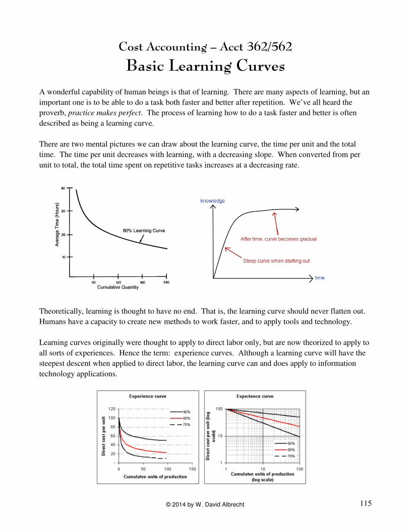
There are two mental pictures we can draw about the learning curve, the time per unit and the total

time. The time per unit decreases with learning, with a decreasing slope. When converted from per

unit to total, the total time spent on repetitive tasks increases at a decreasing rate.

Theoretically, learning is thought to have no end. That is, the learning curve should never flatten out.

Humans have a capacity to create new methods to work faster, and to apply tools and technology.

Learning curves originally were thought to apply to direct labor only, but are now theorized to apply to

all sorts of experiences. Hence the term: experience curves. Although a learning curve will have the

steepest descent when applied to direct labor, the learning curve can and does apply to information

technology applications.

115© 2014 by W. David Albrecht

T. P. Wright wrote (in 1936), the rate of learning for airplane manufacturing was 80% per doubling of

unit output. This means that each time production doubles, the cumulative average time decreases by

20%.

y = axb T = axb+1

(1)

Where:

y = average time per unit

T = total time

a = time required for first unit

x = cumulative number of units produced

b = learning index

b = ln (% learning effect) ÷ ln (2)

The Learning Curve Table

To start the learning on learning curves, we’ll first work on a learning curve table at the doubling

points.

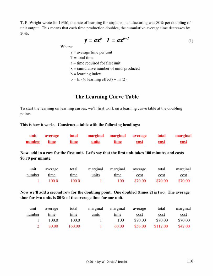
This is how it works. Construct a table with the following headings:

unit average total marginal marginal average total marginal

number time time units time cost cost cost

Now, add in a row for the first unit. Let’s say that the first unit takes 100 minutes and costs

$0.70 per minute.



1 100.0 100.0 1 100 $70.00 $70.00 $70.00

Now we’ll add a second row for the doubling point. One doubled (times 2) is two. The average

time for two units is 80% of the average time for one unit.



1 100.0 100.0 1 100 $70.00 $70.00 $70.00

2 80.00 160.00 1 60.00 $56.00 $112.00 $42.00


Pull out your calculator and use the two equations to verify the average time value and total time value

for row two.

y = axb

b = ln (.8) ÷ ln (2) = !0.22314 ÷ 0.69315 = !0.32192

y = 100*2-0.32192

y = 100*0.8

y = 80.00

T = axb+1

b + 1 = !0.32192 + 1 = +0.67808

y = 100*20.67808

y = 100*1.60

y = 160.00

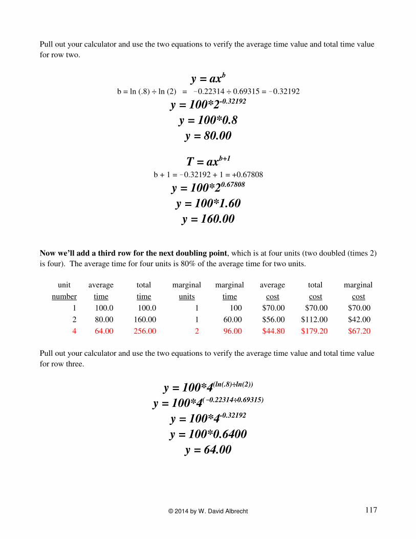
Now we’ll add a third row for the next doubling point, which is at four units (two doubled (times 2)

is four). The average time for four units is 80% of the average time for two units.



1 100.0 100.0 1 100 $70.00 $70.00 $70.00

2 80.00 160.00 1 60.00 $56.00 $112.00 $42.00

4 64.00 256.00 2 96.00 $44.80 $179.20 $67.20


for row three.

y = 100*4(ln(.8)÷ln(2))

y = 100*4(!!!!0.22314÷0.69315)

y = 100*4-0.32192

y = 100*0.6400

y = 64.00


y = 100*40.67808

y = 100*2.5600

y = 256.00

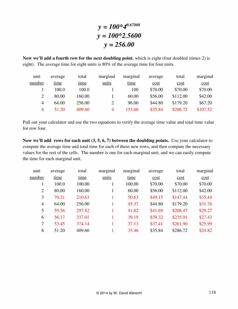
Now we’ll add a fourth row for the next doubling point, which is eight (four doubled (times 2) is

eight). The average time for eight units is 80% of the average time for four units.



1 100.0 100.0 1 100 $70.00 $70.00 $70.00

2 80.00 160.00 1 60.00 $56.00 $112.00 $42.00

4 64.00 256.00 2 96.00 $44.80 $179.20 $67.20

8 51.20 409.60 4 153.60 $35.84 $286.72 $107.52


for row four.

Now we’ll add rows for each unit (3, 5, 6, 7) between the doubling points. Use your calculator to

compute the average time and total time for each of these new rows, and then compute the necessary

values for the rest of the cells. The number is one for each marginal unit, and we can easily compute

the time for each marginal unit.



1 100.0 100.00 1 100.00 $70.00 $70.00 $70.00

2 80.00 160.00 1 60.00 $56.00 $112.00 $42.00

3 70.21 210.63 1 50.63 $49.15 $147.44 $35.44

4 64.00 256.00 1 45.37 $44.80 $179.20 $31.76

5 59.56 297.82 1 41.82 $41.69 $208.47 $29.27

6 56.17 337.01 1 39.19 $39.32 $235.91 $27.43

7 53.45 374.14 1 37.13 $37.41 $261.90 $25.99

8 51.20 409.60 1 35.46 $35.84 $286.72 $24.82


Logarithms and antilogarithms

Now, we need an aside to deal with logarithms. Logarithms are exponents. Another way to think of

it is that a logarithm is the exponent that generates a particular number.

For example, 8 is a number that can result from a mathematical function involving an exponent.

One way of getting the number 8 by way of an exponent is cubing the number 2. This can be

stated as 23, or 2 to the power of 3. The logarithm of 8 is the exponent (or power) of 2 that

generates the number 8. Since 2 to the power of 3 (or 2 cubed, or 2 with an exponent of 3)

generates the number 8, then the logarithm of 8 is 3 (as long as it is the number 2 that we are

taking to some power). The mathematical notation is log2(8) = 3. In words, this reads the log

of 8, given a base of 2, is 3, or 8 results from taking 2 to the power of 3. I think of it using the

latter wording.

We can also get the number 8 by taking the number 10 to some power. We know that 10 to the

zero power is 1, and 10 to the power of 1 is 10. Because 8 is between 1 and 10, if we take 10 to

some power that is between 0 and 1 we will get the number 8. It turns out that 100.90309 = 8.

Turning back to logarithmic notation, we can write log10(8) = 0.90309. In every day English, it

reads that the log of 8, given a base of 10, is 0.90309, or 8 results from taking 10 to the power of

0.90309.

We can also get the number 8 by taking e to some power. e = 2.718281828459. It turns out that

e2.07944 = 8. When we deal with the logarithm with base of e for any number, we are dealing with

natural logarithms. Turning to logarithmic notation, we can write loge(8) = ln(8) = 2.07944.

Why would anyone want to do this? Why do we want to do this?


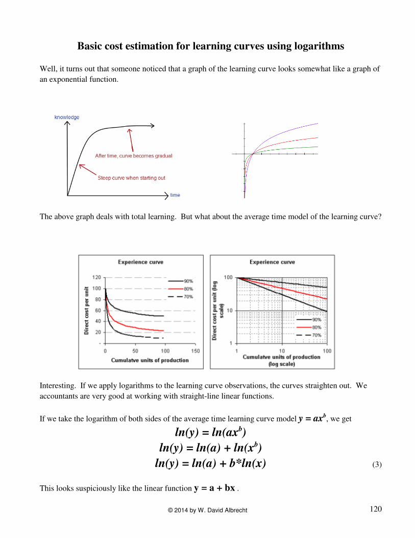
Basic cost estimation for learning curves using logarithms

Well, it turns out that someone noticed that a graph of the learning curve looks somewhat like a graph of

an exponential function.

The above graph deals with total learning. But what about the average time model of the learning curve?

Interesting. If we apply logarithms to the learning curve observations, the curves straighten out. We

accountants are very good at working with straight-line linear functions.

If we take the logarithm of both sides of the average time learning curve model y = axb, we get

ln(y) = ln(axb)

ln(y) = ln(a) + ln(xb)

ln(y) = ln(a) + b*ln(x) (3)

This looks suspiciously like the linear function y = a + bx .


And just a little while ago, we used the “high-low” method. Can it work with learning?

Let’s say that at 100 units the total time is 600 (an average of 6.00). At 200 units the total time is 1,100

(an average of 5.50). What is the learning effect? This is easy because we are at a doubling point. The

learning effect is 5.50 ÷ 6.00 = 91.67%.

But what if we aren’t at a doubling point. Can we use the high-low method to estimate the learning

curve parameters? Of course we can.

Let’s start with a completely new example. At 400 units the total time is 1,200 (an average of 3.00) and

at 1,300 units the total time is 3,400 (an average of 2.61538). Putting it in terms of the cumulative

average time model for the learning curve, we have two equations:

3.00000 = a*400b

2.61538 = a*1,300b

Applying the logarithm function to both sides of each equation, we have:

ln(3.00000) = ln(a) + b*ln(400)

ln(2.61538) = ln(a) + b*ln(1,300)

Or, 1.09861 = ln(a) + b* 5.99146

0.96141 = ln(a) + b*7.17012

subtracting the second equation from the first, we get:

0.13720 = ! 1.17866 * b

b = ! 0.11640

Now to decompose b. Since,


! 0.11640 = ln (% learning effect) ÷ ln (2)

! 0.11640 * ln(2) = ln (% learning effect)

! 0.11640 * 0.69315 = ln (% learning effect)

! 0.08068 = ln (% learning effect)

0.92249 = % learning effect


Once we have the parameter b computed, we can work backwards to get the parameter a. Previously,

we were able to state the two equations as:

1.09861 = ln(a) + b* 5.99146

0.96141 = ln(a) + b*7.17012

Since b = ! 0.11640, we can plug that into either of these two equations to get a. I’ll insert b into the

first equation:

1.09861 = ln(a) + (! 0.11640 * 5.99146)

1.09861 = ln(a) ! 0.69741

1.79602 = ln(a)applying the exp function of the calculator,

6.02562 = a

Putting it all together, we have a 92.249% learning effect (7.751% reduction in cumulative average time

as production doubles), and our estimation equation is:

y = 6.02562x!!!!0.11640

We can use this equation to estimate the cumulative average time at any future amount of activity.

Putting it in terms of the total time model for the learning curve, we have two equations:

1,200 = a*400(b+1)

3,400 = a*1,300(b+1)

Taking the logarithm of each equation, we have:

ln(1,200) = ln(a) + (b+1)*ln(400)

ln(3,400) = ln(a) + (b+1)*ln(1,300)

Or, 7.09008 = ln(a) + b* 5.99146

8.13153 = ln(a) + b*7.17012


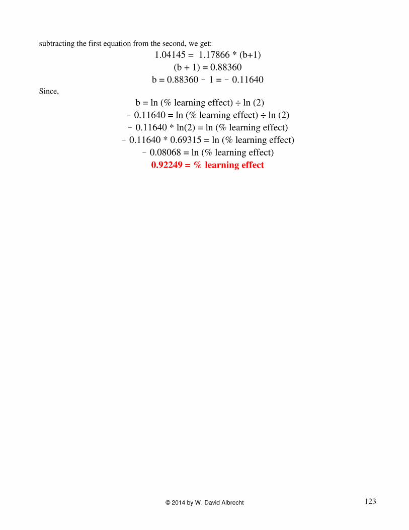
subtracting the first equation from the second, we get:

1.04145 = 1.17866 * (b+1)

(b + 1) = 0.88360

b = 0.88360 ! 1 = ! 0.11640Since,


! 0.11640 = ln (% learning effect) ÷ ln (2)

! 0.11640 * ln(2) = ln (% learning effect)

! 0.11640 * 0.69315 = ln (% learning effect)

! 0.08068 = ln (% learning effect)

0.92249 = % learning effect


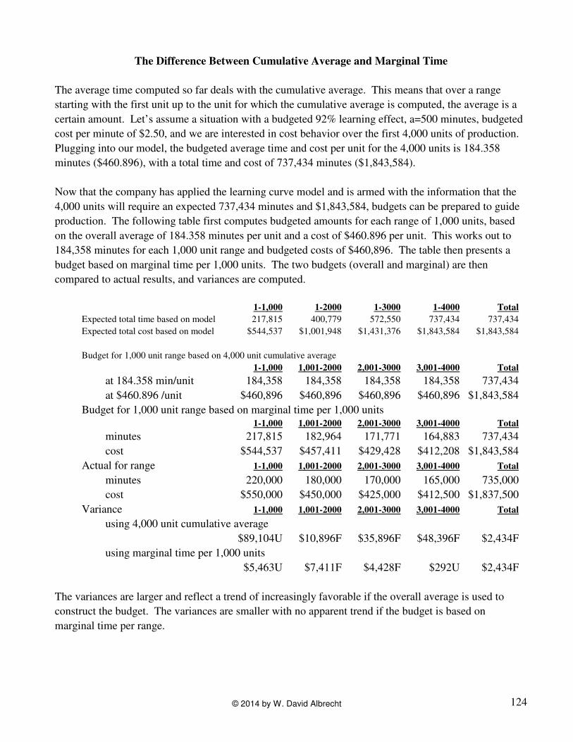
The Difference Between Cumulative Average and Marginal Time

The average time computed so far deals with the cumulative average. This means that over a range

starting with the first unit up to the unit for which the cumulative average is computed, the average is a

certain amount. Let’s assume a situation with a budgeted 92% learning effect, a=500 minutes, budgeted

cost per minute of $2.50, and we are interested in cost behavior over the first 4,000 units of production.

Plugging into our model, the budgeted average time and cost per unit for the 4,000 units is 184.358

minutes ($460.896), with a total time and cost of 737,434 minutes ($1,843,584).

Now that the company has applied the learning curve model and is armed with the information that the

4,000 units will require an expected 737,434 minutes and $1,843,584, budgets can be prepared to guide

production. The following table first computes budgeted amounts for each range of 1,000 units, based

on the overall average of 184.358 minutes per unit and a cost of $460.896 per unit. This works out to

184,358 minutes for each 1,000 unit range and budgeted costs of $460,896. The table then presents a

budget based on marginal time per 1,000 units. The two budgets (overall and marginal) are then

compared to actual results, and variances are computed.

1-1,000 1-2000 1-3000 1-4000 Total

Expected total time based on model 217,815 400,779 572,550 737,434 737,434

Expected total cost based on model $544,537 $1,001,948 $1,431,376 $1,843,584 $1,843,584

Budget for 1,000 unit range based on 4,000 unit cumulative average

1-1,000 1,001-2000 2,001-3000 3,001-4000 Total

at 184.358 min/unit 184,358 184,358 184,358 184,358 737,434

at $460.896 /unit $460,896 $460,896 $460,896 $460,896 $1,843,584

Budget for 1,000 unit range based on marginal time per 1,000 units1-1,000 1,001-2000 2,001-3000 3,001-4000 Total

minutes 217,815 182,964 171,771 164,883 737,434

cost $544,537 $457,411 $429,428 $412,208 $1,843,584

Actual for range 1-1,000 1,001-2000 2,001-3000 3,001-4000 Total

minutes 220,000 180,000 170,000 165,000 735,000

cost $550,000 $450,000 $425,000 $412,500 $1,837,500

Variance 1-1,000 1,001-2000 2,001-3000 3,001-4000 Total

using 4,000 unit cumulative average

$89,104U $10,896F $35,896F $48,396F $2,434F

using marginal time per 1,000 units

$5,463U $7,411F $4,428F $292U $2,434F

The variances are larger and reflect a trend of increasingly favorable if the overall average is used to

construct the budget. The variances are smaller with no apparent trend if the budget is based on

marginal time per range.


Cost Accounting – Acct 362/562

Using Regression to Compute

Learning Curve Parameters

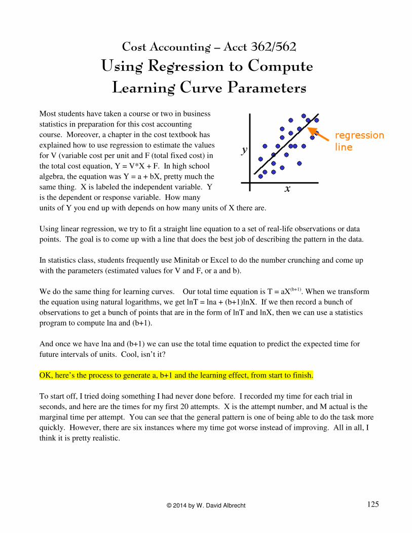
Most students have taken a course or two in business

statistics in preparation for this cost accounting

course. Moreover, a chapter in the cost textbook has

explained how to use regression to estimate the values

for V (variable cost per unit and F (total fixed cost) in

the total cost equation, Y = V*X + F. In high school

algebra, the equation was Y = a + bX, pretty much the

same thing. X is labeled the independent variable. Y

is the dependent or response variable. How many

units of Y you end up with depends on how many units of X there are.

Using linear regression, we try to fit a straight line equation to a set of real-life observations or data

points. The goal is to come up with a line that does the best job of describing the pattern in the data.

In statistics class, students frequently use Minitab or Excel to do the number crunching and come up

with the parameters (estimated values for V and F, or a and b).

We do the same thing for learning curves. Our total time equation is T = aX(b+1). When we transform

the equation using natural logarithms, we get lnT = lna + (b+1)lnX. If we then record a bunch of

observations to get a bunch of points that are in the form of lnT and lnX, then we can use a statistics

program to compute lna and (b+1).

And once we have lna and (b+1) we can use the total time equation to predict the expected time for

future intervals of units. Cool, isn’t it?

OK, here’s the process to generate a, b+1 and the learning effect, from start to finish.

To start off, I tried doing something I had never done before. I recorded my time for each trial in

seconds, and here are the times for my first 20 attempts. X is the attempt number, and M actual is the

marginal time per attempt. You can see that the general pattern is one of being able to do the task more

quickly. However, there are six instances where my time got worse instead of improving. All in all, I

think it is pretty realistic.


X M actual (seconds) X M actual (seconds)

1 201 11 114

2 160 12 112

3 139 13 113

4 137 14 112

5 128 15 107

6 120 16 102

7 116 17 108

8 120 18 100

9 111 19 101

10 115 20 104

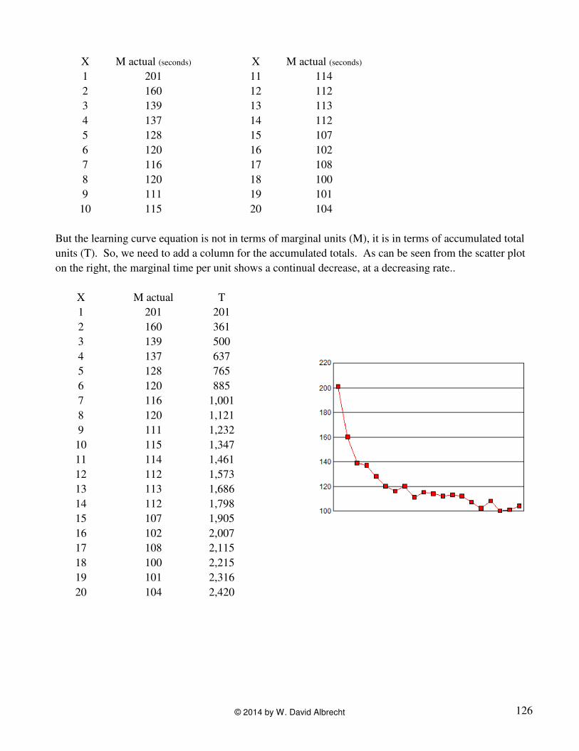
But the learning curve equation is not in terms of marginal units (M), it is in terms of accumulated total

units (T). So, we need to add a column for the accumulated totals. As can be seen from the scatter plot

on the right, the marginal time per unit shows a continual decrease, at a decreasing rate..

X M actual T

1 201 201

2 160 361

3 139 500

4 137 637

5 128 765

6 120 885

7 116 1,001

8 120 1,121

9 111 1,232

10 115 1,347

11 114 1,461

12 112 1,573

13 113 1,686

14 112 1,798

15 107 1,905

16 102 2,007

17 108 2,115

18 100 2,215

19 101 2,316

20 104 2,420


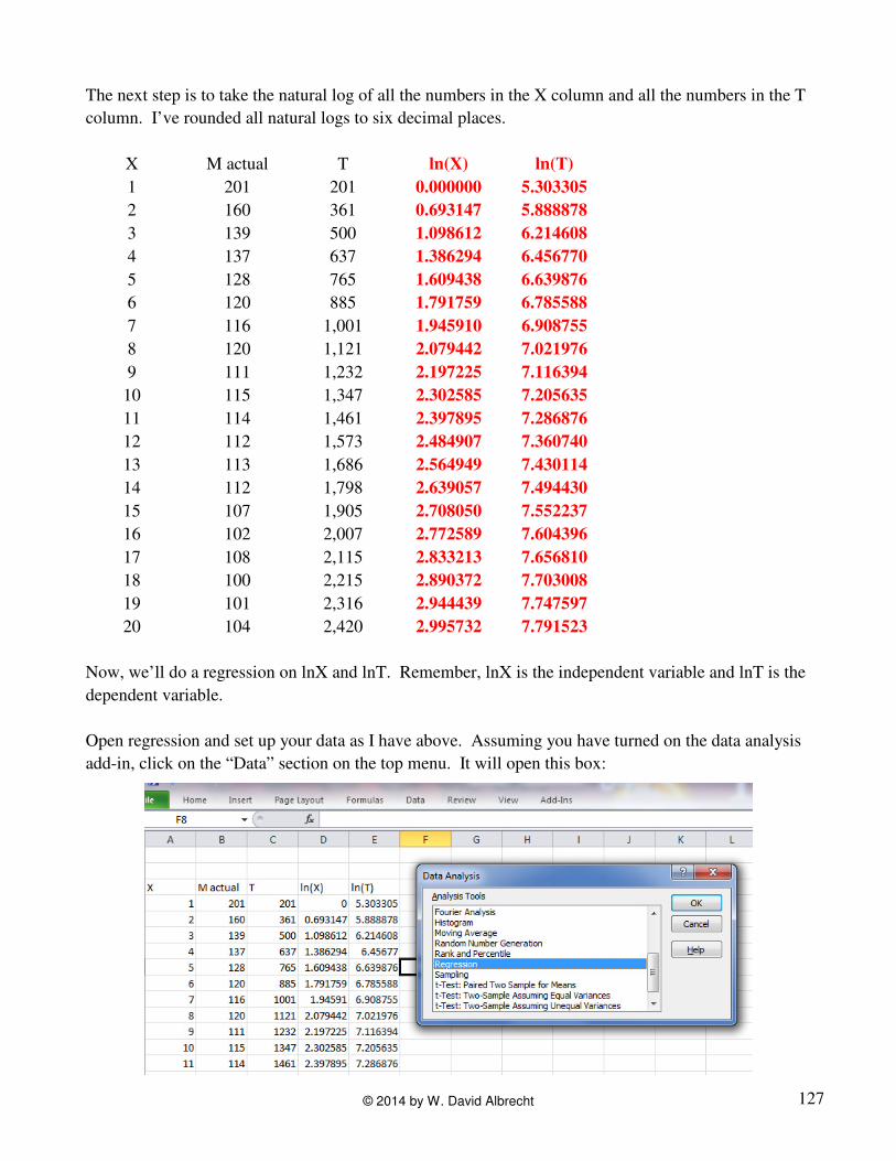
The next step is to take the natural log of all the numbers in the X column and all the numbers in the T

column. I’ve rounded all natural logs to six decimal places.

X M actual T ln(X) ln(T)

1 201 201 0.000000 5.303305

2 160 361 0.693147 5.888878

3 139 500 1.098612 6.214608

4 137 637 1.386294 6.456770

5 128 765 1.609438 6.639876

6 120 885 1.791759 6.785588

7 116 1,001 1.945910 6.908755

8 120 1,121 2.079442 7.021976

9 111 1,232 2.197225 7.116394

10 115 1,347 2.302585 7.205635

11 114 1,461 2.397895 7.286876

12 112 1,573 2.484907 7.360740

13 113 1,686 2.564949 7.430114

14 112 1,798 2.639057 7.494430

15 107 1,905 2.708050 7.552237

16 102 2,007 2.772589 7.604396

17 108 2,115 2.833213 7.656810

18 100 2,215 2.890372 7.703008

19 101 2,316 2.944439 7.747597

20 104 2,420 2.995732 7.791523

Now, we’ll do a regression on lnX and lnT. Remember, lnX is the independent variable and lnT is the

dependent variable.

Open regression and set up your data as I have above. Assuming you have turned on the data analysis

add-in, click on the “Data” section on the top menu. It will open this box:


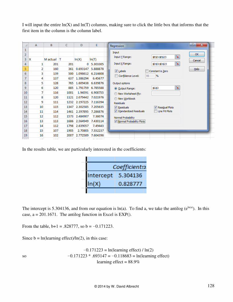
I will input the entire ln(X) and ln(T) columns, making sure to click the little box that informs that the

first item in the column is the column label.

In the results table, we are particularly interested in the coefficients:

The intercept is 5.304136, and from our equation is ln(a). To find a, we take the antilog (eln(a)). In this

case, a = 201.1671. The antilog function in Excel is EXP().

From the table, b+1 = .828777, so b = !0.171223.

Since b = ln(learning effect)/ln(2), in this case:

!0.171223 = ln(learning effect) / ln(2)

so !0.171223 * .693147 = !0.118683 = ln(learning effect)

learning effect = 88.9%


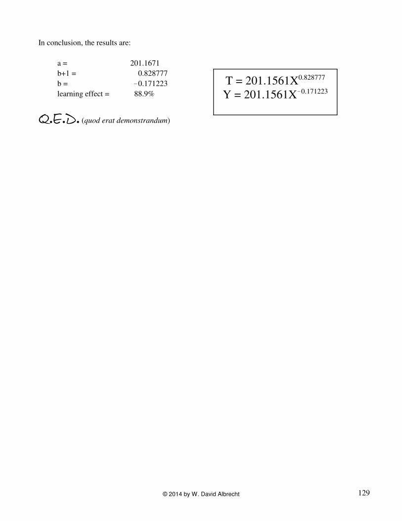
In conclusion, the results are:

a = 201.1671

b+1 = 0.828777

b = !0.171223

learning effect = 88.9%

Q.E.D. (quod erat demonstrandum)

T = 201.1561X0.828777

Y = 201.1561X!0.171223


Documents

Cost Accounting – Acct 362/562 Basic Learning Curves · PDF fileCost Accounting – Acct 362/562 Basic Learning Curves A wonderful capability of human beings is that of learning