Hayley MacphersonDaniel Price & Paul Lasky

Cosmological simulations of large-scale structure with

numerical relativity

arXiv:1807.01711 arXiv:1807.01714

Springel et. al (2005)

Particle methods + Newtonian gravity

Homogeneous background remains homogeneous

Matter cannot interact with spacetime

Cosmological simulations ft. Newton

Gµ⌫ =8⇡G

c4Tµ⌫

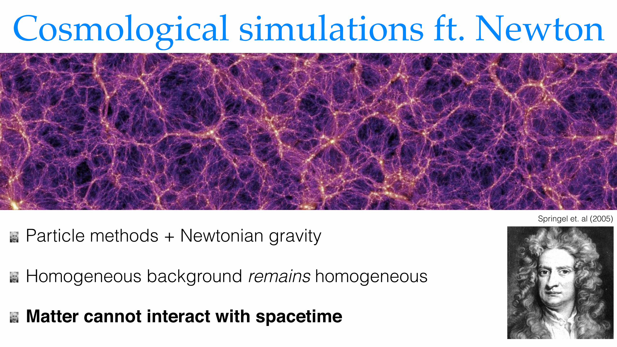
Springel et. al (2005)

Numerical relativity = computationally expensive

No background

Structure DOES interact with & influence spacetime

Cosmological simulations ft. Einstein

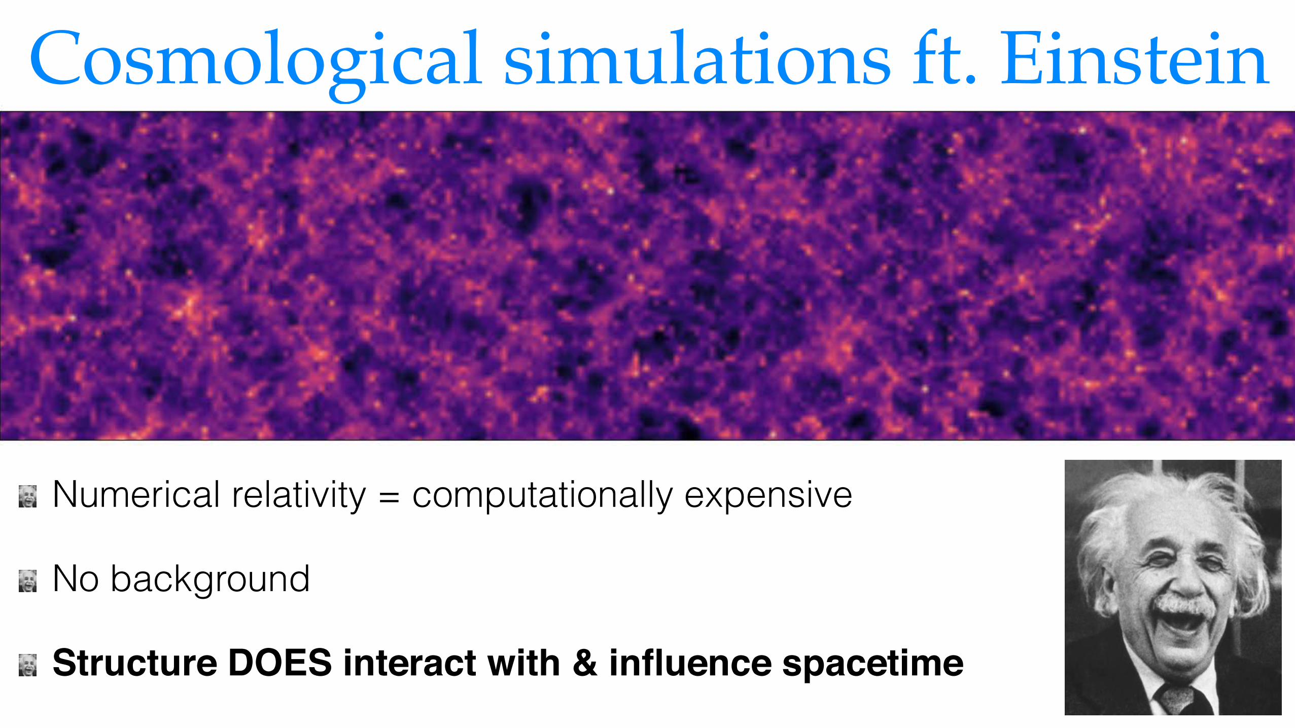
Why?Standard cosmological model is great, and matches most of our observations, but…

Some tensions, e.g. H0 measurement

That pesky 95% of the Universe

Worth exploring whether GR makes a difference

Springel et. al (2005)

How?

Cosmology with numerical relativity began with:

Giblin et al. (2016), Bentivegna & Bruni (2016), Macpherson et al. (2017)

Our way

Image: David Liptai

Open-source code CACTUS

Einstein Toolkit: mainly used for black holes & neutron stars

We wrote FLRWSolver to initialise cosmological spacetimes (arXiv:1611.05447)

Hydrodynamics on a grid (no particles)

Matter dominated —> no Lambda

Evolved in longitudinal (Poisson) gauge

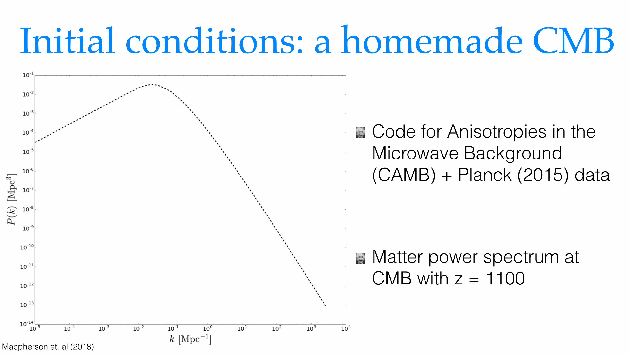
Initial conditions: a homemade CMB

Code for Anisotropies in the Microwave Background (CAMB) + Planck (2015) data

Matter power spectrum at CMB with z = 1100

Macpherson et. al (2018)

Create Gaussian random field

This gives density perturbation

Sample P(k) to Nyquist frequency:

Initial conditions: a homemade CMB

�min ⇠ 2�x

Macpherson et. al (2018)

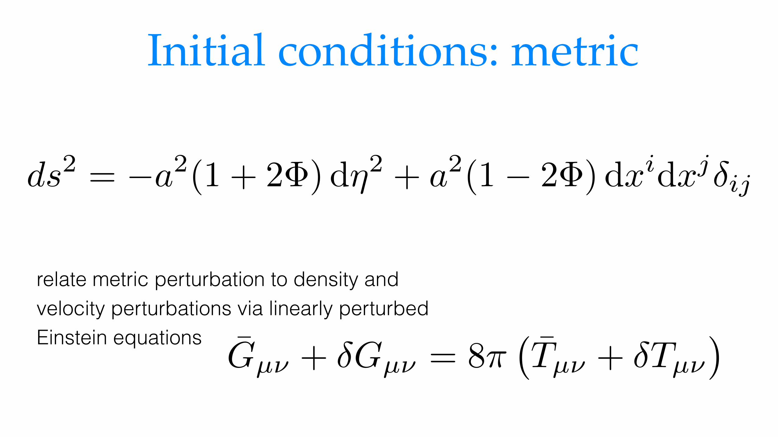
Initial conditions: metric

ds

2 = �a

2(1 + 2�) d⌘2 + a

2(1� 2�) dxidxj�ij

relate metric perturbation to density and velocity perturbations via linearly perturbed Einstein equations

Gµ⌫ + �Gµ⌫ = 8⇡�Tµ⌫ + �Tµ⌫

�

Initial conditions

�⇢/⇢ � |v|

1Gpc

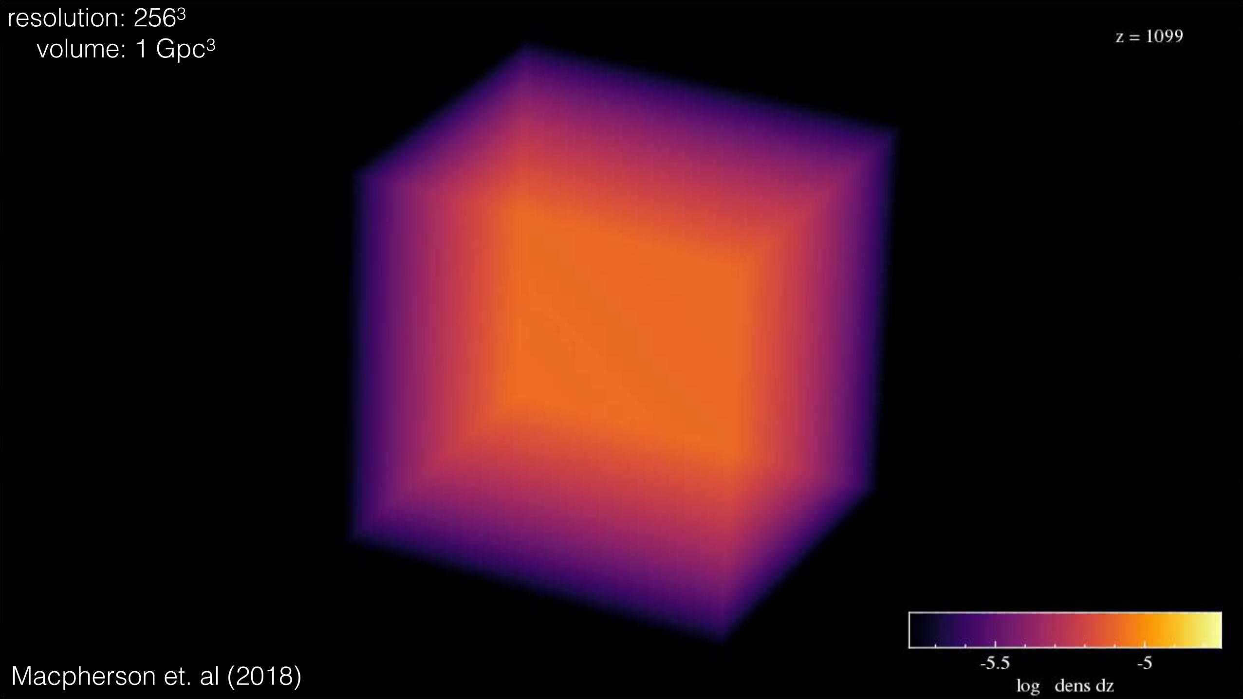
resolution: 2563 volume: 1 Gpc3

Macpherson et. al (2018)

What can we do with this?Averaging & backreaction

Ray tracing & Hubble diagrams

other observables

ISW effect

Weyl tensor & vector modes

a lot more we haven’t thought of yet…

Macpherson et. al (2018)

What can we do with this?Averaging & backreaction

Ray tracing & Hubble diagrams

other observables

ISW effect

Weyl tensor & vector modes

a lot more we haven’t thought of yet…

Macpherson et. al (2018)

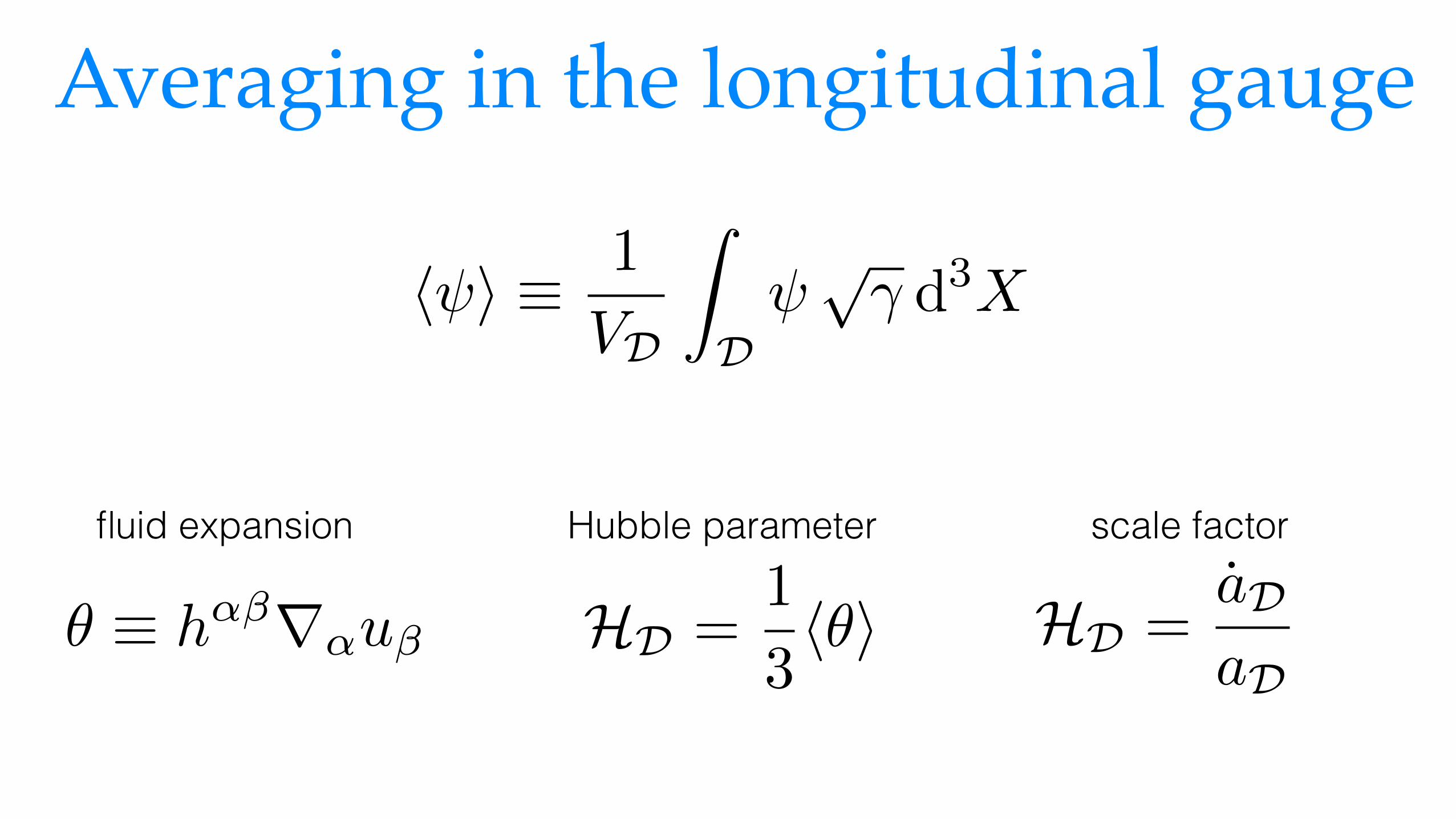
Averaging in the longitudinal gauge

HD =1

3h✓i HD =

aDaD

✓ ⌘ h↵�r↵u�

fluid expansion Hubble parameter scale factor

h i ⌘ 1

VD

Z

D p� d3X

Averaging in the longitudinal gauge

averaged Hamiltonian constraint

backreaction terms

6HD2 = 16⇡h⇢i �RD �QD + LD

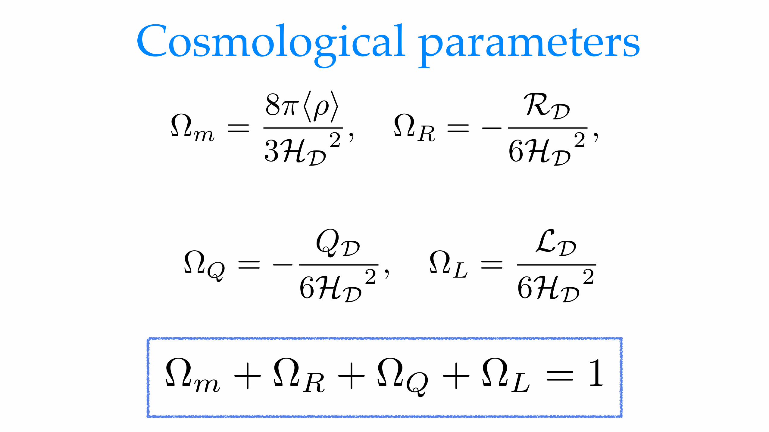
Cosmological parameters

⌦m =8⇡h⇢i3HD

2 , ⌦R = � RD

6HD2 ,

⌦Q = � QD

6HD2 , ⌦L =

LD

6HD2

⌦m + ⌦R + ⌦Q + ⌦L = 1

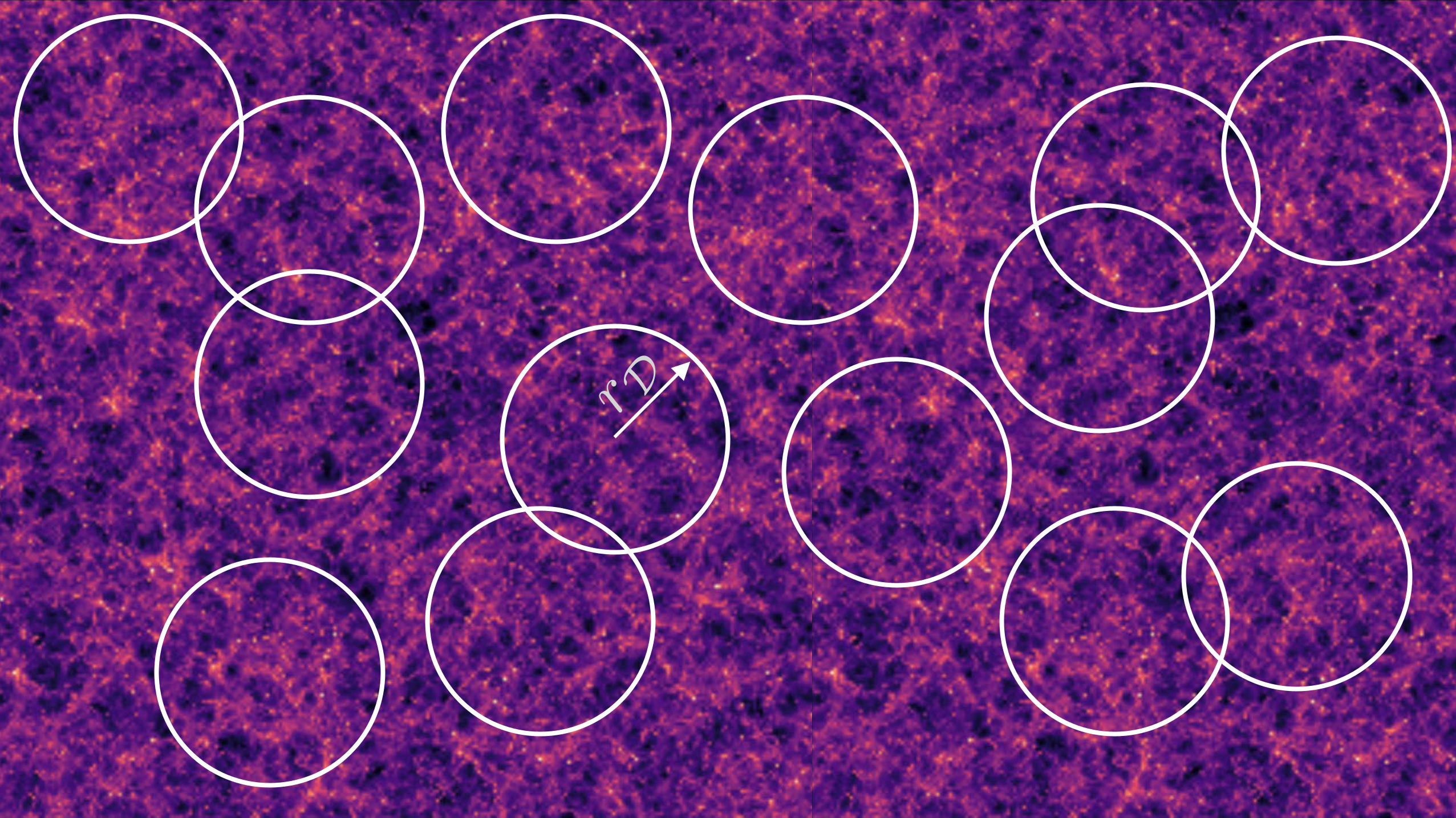
r D

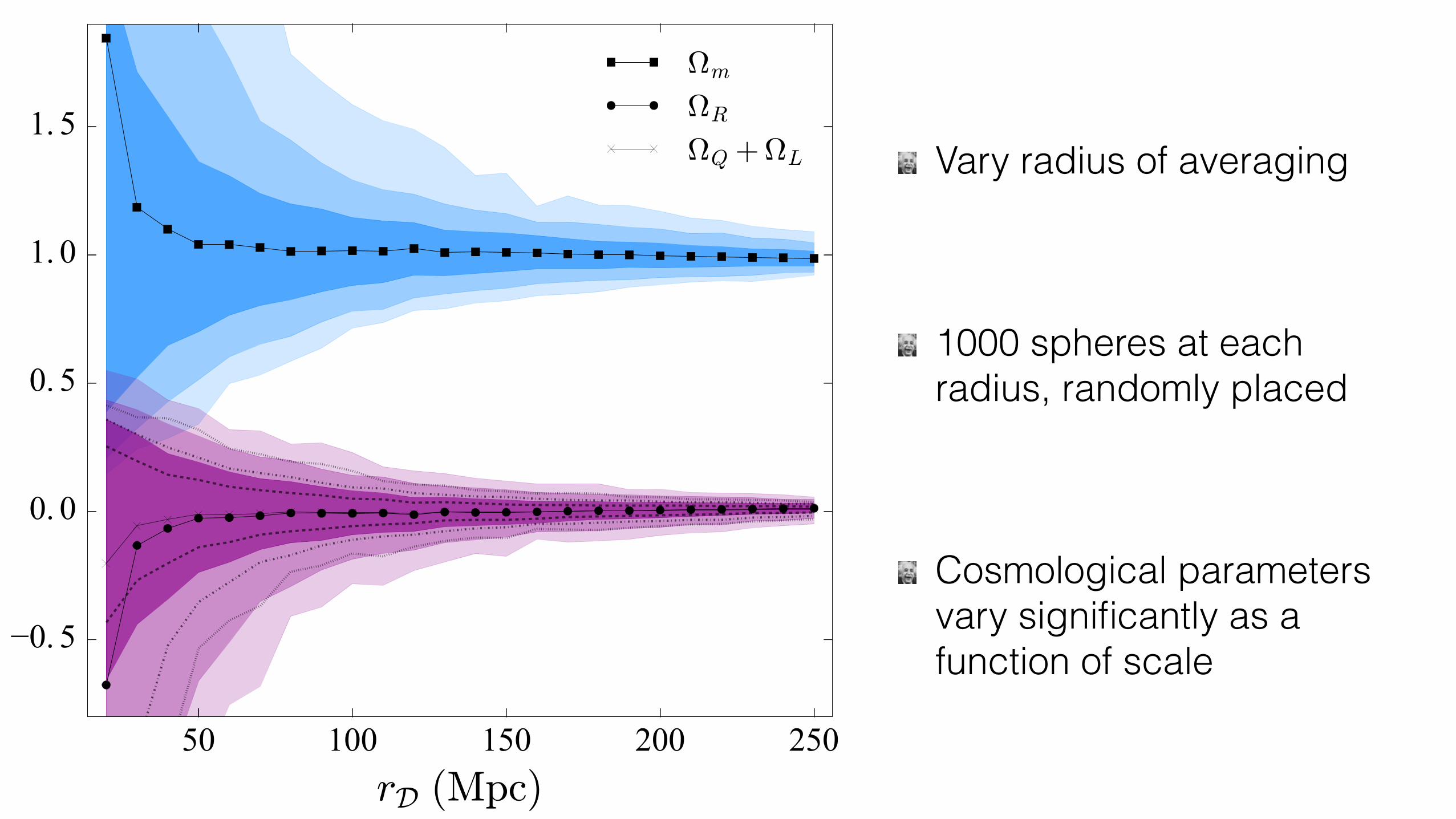
Vary radius of averaging

1000 spheres at each radius, randomly placed

Cosmological parameters vary significantly as a function of scale

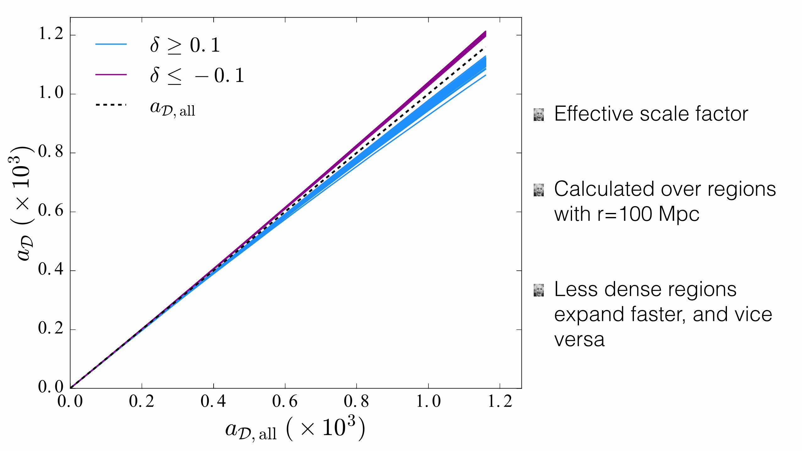
Effective scale factor

Calculated over regions with r=100 Mpc

Less dense regions expand faster, and vice versa

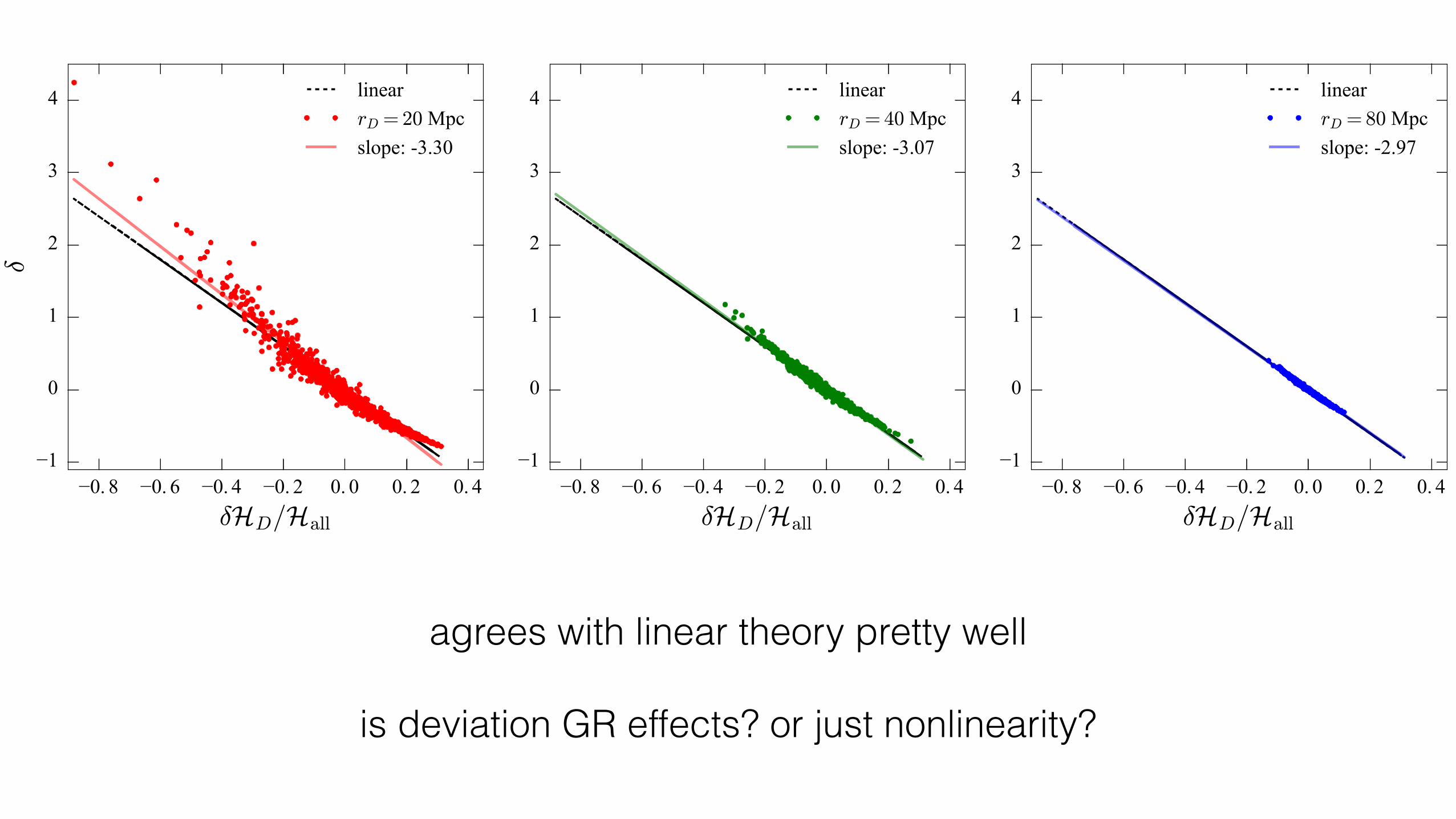
agrees with linear theory pretty well

is deviation GR effects? or just nonlinearity?

Caveats…We treat Dark Matter as a fluid — using a grid approximation

(particles would be better)

We assume averages over a purely spatial volume (no light cone

averaging)

at z=0, implies all variations are upper limits

Currently limited in resolution

ConclusionsCosmological simulations with numerical relativity

We’ve got a cosmic web!

Globally we find no backreaction effects

Backreaction and curvature can be significant on small scales (<100 Mpc)

Very near future: ray tracing and real observables

Extra stuff

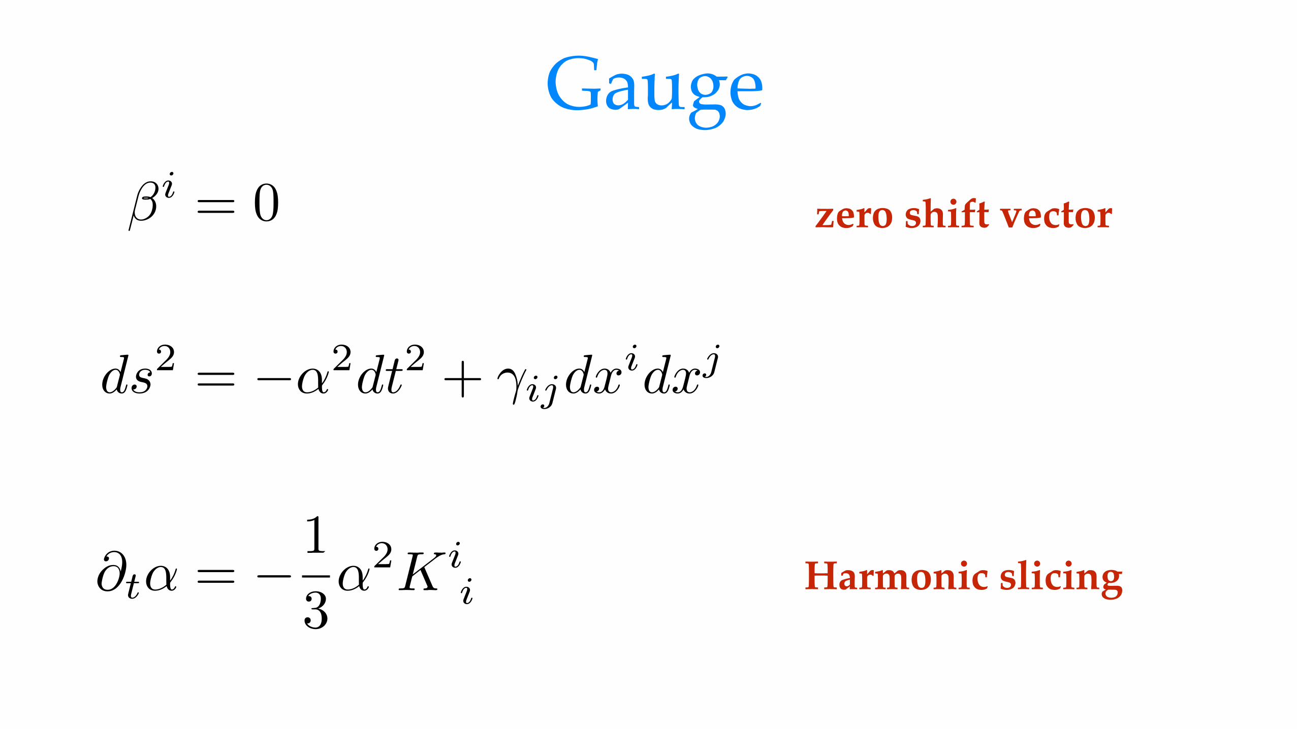
Gauge�

i = 0

ds

2 = �↵

2dt

2 + �ijdxidx

j

@t↵ = �1

3↵

2K

ii

zero shift vector

Harmonic slicing

Constraints