Cosmic Star-FormationHistory arXiv:1403.0007v3 [astro-ph

arX

iv:1

403.

0007

v3 [

astr

o-ph

.CO

] 1

3 Ju

n 20

14

Cosmic Star-Formation History

Piero Madau

Department of Astronomy and Astrophysics, University of California, Santa Cruz,

California 95064; email: [email protected]

Mark Dickinson

National Optical Astronomy Observatory, Tucson, Arizona 85719; email:

[email protected]

Key Words

cosmology, galaxy formation, evolution, star formation, stellar populations

Abstract

Over the past two decades, an avalanche of data from multiwavelength imaging and spec-

troscopic surveys has revolutionized our view of galaxy formation and evolution. Here we

review the range of complementary techniques and theoretical tools that allow astronomers

to map the cosmic history of star formation, heavy element production, and reionization

of the Universe from the cosmic “dark ages” to the present epoch. A consistent picture is

emerging, whereby the star-formation rate density peaked approximately 3.5 Gyr after the

Big Bang, at z ≈ 1.9, and declined exponentially at later times, with an e-folding timescale

of 3.9 Gyr. Half of the stellar mass observed today was formed before a redshift z = 1.3.

About 25% formed before the peak of the cosmic star-formation rate density, and another

25% formed after z = 0.7. Less than ∼ 1% of today’s stars formed during the epoch of

reionization. Under the assumption of a universal initial mass function, the global stellar

mass density inferred at any epoch matches reasonably well the time integral of all the pre-

ceding star-formation activity. The comoving rates of star formation and central black hole

accretion follow a similar rise and fall, offering evidence for co-evolution of black holes and

their host galaxies. The rise of the mean metallicity of the Universe to about 0.001 solar by

z = 6, one Gyr after the Big Bang, appears to have been accompanied by the production of

fewer than ten hydrogen Lyman-continuum photons per baryon, a rather tight budget for

cosmological reionization.

CONTENTS

INTRODUCTION . . . . . . . . . . . . . . . . . . . . . . . . . . . . . . . . . . . . . . . . . . 2

THE EQUATIONS OF COSMIC CHEMICAL EVOLUTION . . . . . . . . . . . . . . . . . . 5

MEASURING MASS FROM LIGHT . . . . . . . . . . . . . . . . . . . . . . . . . . . . . . . 7Star-Formation Rates . . . . . . . . . . . . . . . . . . . . . . . . . . . . . . . . . . . . . . . 11

“Weighing” Stellar Mass . . . . . . . . . . . . . . . . . . . . . . . . . . . . . . . . . . . . . 22

Cosmic Star-Formation History 1

http://arxiv.org/abs/1403.0007v3

Annu. Rev. Astron. Astrophys. 2013 1056-8700/97/0610-00

TRACING THE GALAXY EMISSION HISTORY WITH LARGE SURVEYS . . . . . . . . 25UV Surveys . . . . . . . . . . . . . . . . . . . . . . . . . . . . . . . . . . . . . . . . . . . . . 25

Infrared Surveys . . . . . . . . . . . . . . . . . . . . . . . . . . . . . . . . . . . . . . . . . . 29

Emission Line Surveys . . . . . . . . . . . . . . . . . . . . . . . . . . . . . . . . . . . . . . . 35

Radio Surveys . . . . . . . . . . . . . . . . . . . . . . . . . . . . . . . . . . . . . . . . . . . 37

Stellar Mass Density Surveys . . . . . . . . . . . . . . . . . . . . . . . . . . . . . . . . . . . 38

The State of the Art, and What’s Wrong with It . . . . . . . . . . . . . . . . . . . . . . . . 41

FROM OBSERVATIONS TO GENERAL PRINCIPLES . . . . . . . . . . . . . . . . . . . . . 45Star-Formation Density . . . . . . . . . . . . . . . . . . . . . . . . . . . . . . . . . . . . . . 45

Core-Collapse Supernova Rate . . . . . . . . . . . . . . . . . . . . . . . . . . . . . . . . . . 49

Stellar Mass Density . . . . . . . . . . . . . . . . . . . . . . . . . . . . . . . . . . . . . . . . 50

Fossil Cosmology . . . . . . . . . . . . . . . . . . . . . . . . . . . . . . . . . . . . . . . . . . 53

The Global Specific Star Formation Rate . . . . . . . . . . . . . . . . . . . . . . . . . . . . . 54

Cosmic Metallicity . . . . . . . . . . . . . . . . . . . . . . . . . . . . . . . . . . . . . . . . . 56

Black Hole Accretion History . . . . . . . . . . . . . . . . . . . . . . . . . . . . . . . . . . . 58

First Light and Cosmic Reionization . . . . . . . . . . . . . . . . . . . . . . . . . . . . . . . 59

CONCLUDING REMARKS . . . . . . . . . . . . . . . . . . . . . . . . . . . . . . . . . . . . 62

DISCLOSURE STATEMENT . . . . . . . . . . . . . . . . . . . . . . . . . . . . . . . . . . . . 65

ACKNOWLEDGMENTS . . . . . . . . . . . . . . . . . . . . . . . . . . . . . . . . . . . . . . 65

1 INTRODUCTION

The origin and evolution of galaxies are among the most intriguing and complex chapters

in the formation of cosmic structure, and observations in this field have accumulated at

an astonishing pace. Multiwavelength imaging surveys with the Hubble (HST) and Spitzer

space telescopes and ground-based facilities, together with spectroscopic follow-up with 8-

m-class telescopes, have led to the discovery of galaxies with confirmed redshifts as large as

z = 7.5 (Finkelstein et al. 2013), as well as compelling photometric candidates as far back

as z ≈ 11 (Coe et al. 2013) when the Universe was only 3% of its current age. Following

the seminal work of Steidel et al. (1995), color-selection criteria that are sensitive to the

presence of intergalactic H I absorption features in the spectral energy distribution (SED) of

distant sources have been used to build increasingly large samples of star-forming galaxies

at 2.5 ∼< z ∼

< 9 (e.g., Madau et al. 1996, Steidel et al. 2003, Giavalisco et al. 2004a, Bouwens

et al. 2011b). Infrared (IR)-optical color selection criteria efficiently isolate both actively

star-forming and passively evolving galaxies at z ≈ 2 (Franx et al. 2003, Daddi et al. 2004).

Photometric redshifts have become an unavoidable tool for placing faint galaxies onto a

cosmic timeline. Spitzer, Herschel, and submillimeter telescopes have revealed that dusty

galaxies with star-formation rates (SFRs) of order 100 M⊙ year−1 or more were abundant

when the Universe was only 2–3 Gyr old (Barger et al. 1998, Daddi et al. 2005, Gruppioni

et al. 2013). Deep near-infrared (NIR) observations are now commonly used to select

galaxies on the basis of their optical rest-frame light and to chart the evolution of the global

stellar mass density (SMD) at 0 < z < 3 (Dickinson et al. 2003). The Galaxy Evolution

Explorer (GALEX) satellite has quantified the ultraviolet galaxy luminosity function (LF)

of galaxies in the local Universe and its evolution at z ∼< 1. Ground-based observations

and, subsequently, UV and IR data from GALEX and Spitzer have confirmed that star-

formation activity was significantly higher in the past (Lilly et al. 1996, Schiminovich et al.

2005, Le Floc’h et al. 2005). In the local Universe, various galaxy properties (colors, surface

mass densities, and concentrations) have been observed by the Sloan Digital Sky Survey

(SDSS) to be “bimodal” around a transitional stellar mass of 3×1010 M⊙ (Kauffmann et al.

2

2003), showing a clear division between faint, blue, active galaxies and bright, red, passive

systems. The number and total stellar mass of blue galaxies appear to have remained nearly

constant since z ∼ 1, whereas those of red galaxies (around L∗) have been rising (Faber

et al. 2007). At redshifts 0 < z < 2 at least, and perhaps earlier, most star-forming galaxies

are observed to obey a relatively tight “main-sequence” correlation between their SFRs and

stellar masses (Brinchmann et al. 2004, Noeske et al. 2007, Elbaz et al. 2007, Daddi et al.

2007). A minority of starburst galaxies have elevated SFRs above this main sequence as

well as a growing population of quiescent galaxies that fall below it.

With the avalanche of new data, galaxy taxonomy has been enriched by the addition of

new acronyms such as LBGs, LAEs, EROs, BzKs, DRGs, DOGs, LIRGs, ULIRGs, and

SMGs. Making sense of it all and fitting it together into a coherent picture remains one

of astronomy’s great challenges, in part because of the observational difficulty of tracking

continuously transforming galaxy sub-populations across cosmic time and in part because

theory provides only a partial interpretative framework. The key idea of standard cosmo-

logical scenarios is that primordial density fluctuations grow by gravitational instability

driven by cold, collisionless dark matter, leading to a “bottom-up” ΛCDM (cold dark mat-

ter) scenario of structure formation (Peebles 1982). Galaxies form hierarchically: Low-mass

objects (“halos”) collapse earlier and merge to form increasingly larger systems over time

– from ultra-faint dwarfs to clusters of galaxies (Blumenthal et al. 1984). Ordinary matter

in the Universe follows the dynamics dictated by the dark matter until radiative, hydro-

dynamic, and star-formation processes take over (White & Rees 1978). The “dark side”

of galaxy formation can be modeled with high accuracy and has been explored in detail

through N-body numerical simulations of increasing resolution and size (e.g., Davis et al.

1985, Dubinski & Carlberg 1991, Moore et al. 1999, Springel et al. 2005, 2008, Diemand

et al. 2008, Stadel et al. 2009, Klypin et al. 2011). However, the same does not hold for

the baryons. Several complex processes are still poorly understood, for example, baryonic

dissipation inside evolving CDM halos, the transformation of cold gas into stars, the for-

mation of disks and spheroids, the chemical enrichment of gaseous material on galactic

and intergalactic scales, and the role played by “feedback” [the effect of the energy input

from stars, supernovae (SNe), and massive black holes on their environment] in regulating

star formation and generating galactic outflows. The purely phenomenological treatment of

complex physical processes that is at the core of semi-analytic schemes of galaxy formation

(e.g., White & Frenk 1991, Kauffmann et al. 1993, Somerville & Primack 1999, Cole et al.

2000) and – at a much higher level of realism – the “subgrid modeling” of star formation

and stellar feedback that must be implemented even in the more accurate cosmological

hydrodynamic simulations (e.g., Katz et al. 1996, Yepes et al. 1997, Navarro & Steinmetz

2000, Springel & Hernquist 2003, Keres al. 2005, Ocvirk et al. 2008, Governato et al. 2010,

Guedes et al. 2011, Hopkins et al. 2012, Kuhlen et al. 2012, Zemp et al. 2012, Agertz et al.

2013) are sensitive to poorly determined parameters and suffer from various degeneracies,

a weakness that has traditionally prevented robust predictions to be made in advance of

specific observations.

Ideally, an in-depth understanding of galaxy evolution would encompass the full sequence

of events that led from the formation of the first stars after the end of the cosmic dark ages

to the present-day diversity of forms, sizes, masses, colors, luminosities, metallicities, and

clustering properties of galaxies. This is a daunting task, and it is perhaps not surprising

that an alternative way to look at and interpret the bewildering variety of galaxy data

has become very popular in the past two decades. The method focuses on the emission

properties of the galaxy population as a whole, traces the evolution with cosmic time of the


galaxy luminosity density from the far-UV (FUV) to the far-infrared (FIR), and offers the

prospect of an empirical determination of the global history of star formation and heavy

element production of the Universe, independently of the complex evolutionary phases of

individual galaxy subpopulations. The modern version of this technique relies on some

basic properties of stellar populations and dusty starburst galaxies:

1. The UV-continuum emission in all but the oldest galaxies is dominated by short-

lived massive stars. Therefore, for a given stellar initial mass function (IMF) and

dust content, it is a direct measure of the instantaneous star-formation rate density

(SFRD).

2. The rest-frame NIR light is dominated by near-solar-mass evolved stars that make up

the bulk of a galaxy’s stellar mass and can then be used as a tracer of the total SMD.

3. Interstellar dust preferentially absorbs UV light and re-radiates it in the thermal IR,

so that the FIR emission of dusty starburst galaxies can be a sensitive tracer of young

stellar populations and the SFRD.

By modeling the emission history of all stars in the Universe at UV, optical, and IR

wavelengths from the present epoch to z ≈ 8 and beyond, one can then shed light on some

key questions in galaxy formation and evolution studies: Is there a characteristic cosmic

epoch of the formation of stars and heavy elements in galaxies? What fraction of the

luminous baryons observed today were already locked into galaxies at early times? Are

the data consistent with a universal IMF? Do galaxies reionize the Universe at a redshift

greater than 6? Can we account for all the metals produced by the global star-formation

activity from the Big Bang to the present? How does the cosmic history of star formation

compare with the history of mass accretion onto massive black holes as traced by luminous

quasars?

This review focuses on the range of observations, methods, and theoretical tools that are

allowing astronomers to map the rate of transformation of gas into stars in the Universe,

from the cosmic dark ages to the present epoch. Given the limited space available, it is

impossible to provide a thorough survey of such a huge community effort without leaving

out significant contributions or whole subfields. We have therefore tried to refer only briefly

to earlier findings, and present recent observations in more detail, limiting the number of

studies cited and highlighting key research areas. In doing so, we hope to provide a man-

ageable overview of how the field has developed and matured in line with new technological

advances and theoretical insights, and of the questions with which astronomers still struggle

nowadays.

The remainder of this review is organized as follows. The equations of cosmic chemical

evolution that govern the consumption of gas into stars and the formation and dispersal of

heavy elements in the Universe as a whole are given in Section 2. We turn to the topic of

measuring mass from light, and draw attention to areas of uncertainty in Section 3. Large

surveys, key data sets and the analyses thereof are highlighted in Section 4. An up-to-date

determination of the star-formation history (SFH) of the Universe is provided and its main

implications are discussed in Serction 5. Finally, we summarize our conclusions in Section

6. Unless otherwise stated, all results presented here will assume a “cosmic concordance

cosmology” with parameters (ΩM ,ΩΛ,Ωb, h) = (0.3, 0.7, 0.045, 0.7).

4 P. Madau & M. Dickinson

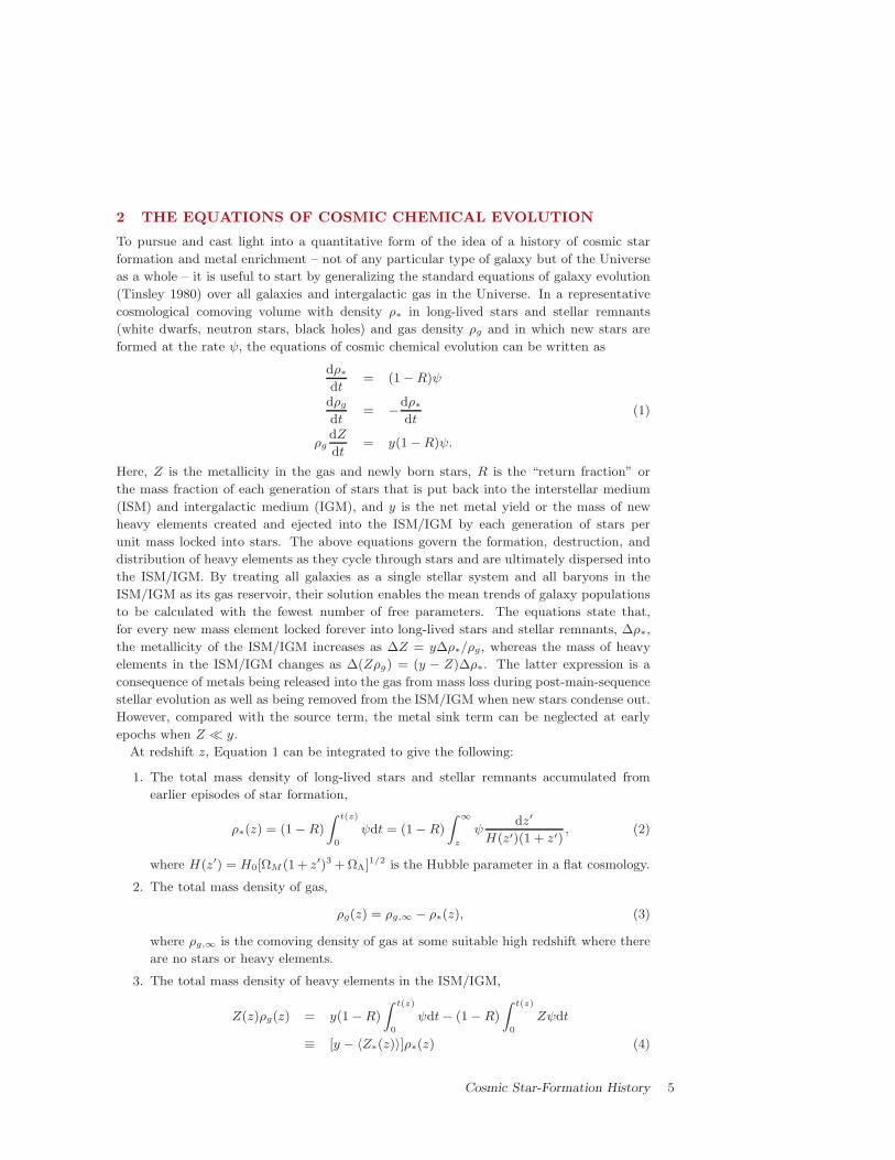
2 THE EQUATIONS OF COSMIC CHEMICAL EVOLUTION

To pursue and cast light into a quantitative form of the idea of a history of cosmic star

formation and metal enrichment – not of any particular type of galaxy but of the Universe

as a whole – it is useful to start by generalizing the standard equations of galaxy evolution

(Tinsley 1980) over all galaxies and intergalactic gas in the Universe. In a representative

cosmological comoving volume with density ρ∗ in long-lived stars and stellar remnants

(white dwarfs, neutron stars, black holes) and gas density ρg and in which new stars are

formed at the rate ψ, the equations of cosmic chemical evolution can be written as

dρ∗dt

= (1−R)ψ

dρgdt

= −dρ∗dt

(1)

ρgdZ

dt= y(1−R)ψ.

Here, Z is the metallicity in the gas and newly born stars, R is the “return fraction” or

the mass fraction of each generation of stars that is put back into the interstellar medium

(ISM) and intergalactic medium (IGM), and y is the net metal yield or the mass of new

heavy elements created and ejected into the ISM/IGM by each generation of stars per

unit mass locked into stars. The above equations govern the formation, destruction, and

distribution of heavy elements as they cycle through stars and are ultimately dispersed into

the ISM/IGM. By treating all galaxies as a single stellar system and all baryons in the

ISM/IGM as its gas reservoir, their solution enables the mean trends of galaxy populations

to be calculated with the fewest number of free parameters. The equations state that,

for every new mass element locked forever into long-lived stars and stellar remnants, ∆ρ∗,

the metallicity of the ISM/IGM increases as ∆Z = y∆ρ∗/ρg, whereas the mass of heavy

elements in the ISM/IGM changes as ∆(Zρg) = (y − Z)∆ρ∗. The latter expression is a

consequence of metals being released into the gas from mass loss during post-main-sequence

stellar evolution as well as being removed from the ISM/IGM when new stars condense out.

However, compared with the source term, the metal sink term can be neglected at early

epochs when Z ≪ y.

At redshift z, Equation 1 can be integrated to give the following:

1. The total mass density of long-lived stars and stellar remnants accumulated from

earlier episodes of star formation,

ρ∗(z) = (1−R)

∫ t(z)

0

ψdt = (1−R)

∫ ∞

z

ψdz′

H(z′)(1 + z′), (2)

where H(z′) = H0[ΩM (1+ z′)3 +ΩΛ]1/2 is the Hubble parameter in a flat cosmology.

2. The total mass density of gas,

ρg(z) = ρg,∞ − ρ∗(z), (3)

where ρg,∞ is the comoving density of gas at some suitable high redshift where there

are no stars or heavy elements.

3. The total mass density of heavy elements in the ISM/IGM,

Z(z)ρg(z) = y(1−R)

∫ t(z)

0

ψdt− (1−R)

∫ t(z)

0

Zψdt

≡ [y − 〈Z∗(z)〉]ρ∗(z) (4)


where the term 〈Z∗〉ρ∗ is the total metal content of stars and remnants at that redshift.

Note that the instantaneous total metal ejection rate, EZ, is the sum of a recycle term

and a creation term (Maeder 1992),

EZ = ZRψ + y(1−R)ψ, (5)

where the first term is the amount of heavy elements initially lost from the ISM when

stars formed that are now being re-released, and the second represents the new metals

synthesized by stars and released during mass loss.

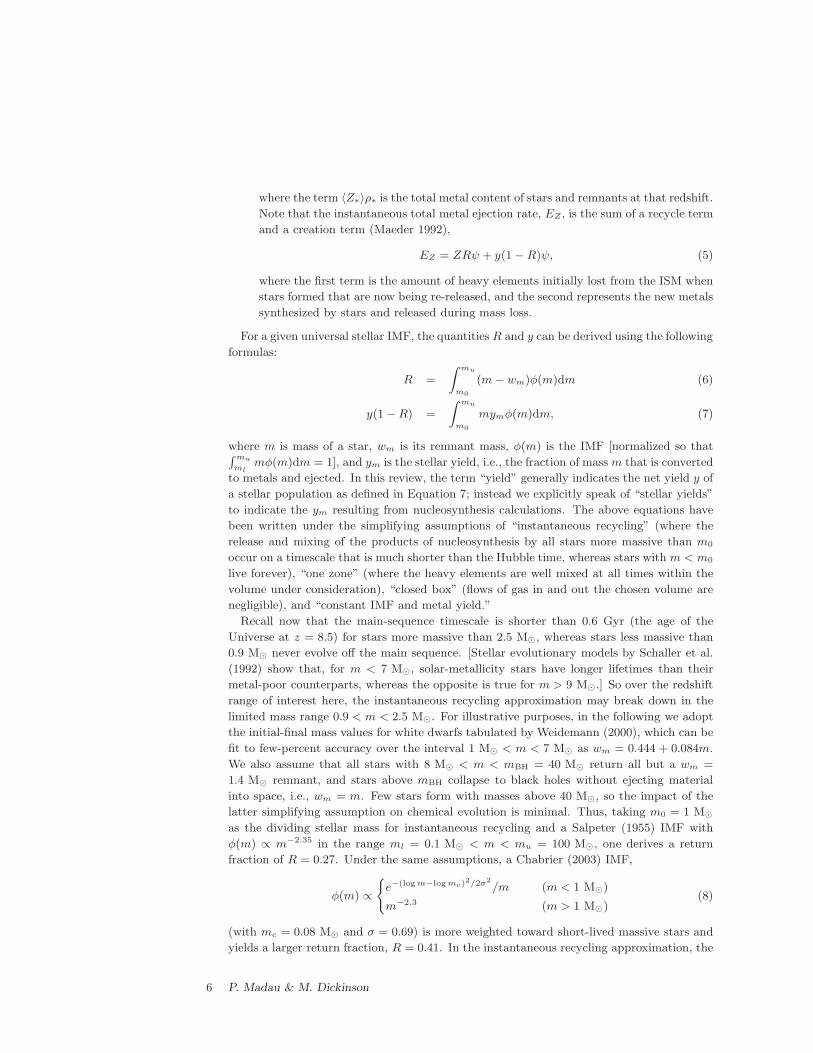
For a given universal stellar IMF, the quantities R and y can be derived using the following

formulas:

R =

∫ mu

m0

(m− wm)φ(m)dm (6)

y(1−R) =

∫ mu

m0

mymφ(m)dm, (7)

where m is mass of a star, wm is its remnant mass, φ(m) is the IMF [normalized so that∫mu

ml

mφ(m)dm = 1], and ym is the stellar yield, i.e., the fraction of massm that is converted

to metals and ejected. In this review, the term “yield” generally indicates the net yield y of

a stellar population as defined in Equation 7; instead we explicitly speak of “stellar yields”

to indicate the ym resulting from nucleosynthesis calculations. The above equations have

been written under the simplifying assumptions of “instantaneous recycling” (where the

release and mixing of the products of nucleosynthesis by all stars more massive than m0

occur on a timescale that is much shorter than the Hubble time, whereas stars with m < m0

live forever), “one zone” (where the heavy elements are well mixed at all times within the

volume under consideration), “closed box” (flows of gas in and out the chosen volume are

negligible), and “constant IMF and metal yield.”

Recall now that the main-sequence timescale is shorter than 0.6 Gyr (the age of the

Universe at z = 8.5) for stars more massive than 2.5 M⊙, whereas stars less massive than

0.9 M⊙ never evolve off the main sequence. [Stellar evolutionary models by Schaller et al.

(1992) show that, for m < 7 M⊙, solar-metallicity stars have longer lifetimes than their

metal-poor counterparts, whereas the opposite is true for m > 9 M⊙.] So over the redshift

range of interest here, the instantaneous recycling approximation may break down in the

limited mass range 0.9 < m < 2.5 M⊙. For illustrative purposes, in the following we adopt

the initial-final mass values for white dwarfs tabulated by Weidemann (2000), which can be

fit to few-percent accuracy over the interval 1 M⊙ < m < 7 M⊙ as wm = 0.444 + 0.084m.

We also assume that all stars with 8 M⊙ < m < mBH = 40 M⊙ return all but a wm =

1.4 M⊙ remnant, and stars above mBH collapse to black holes without ejecting material

into space, i.e., wm = m. Few stars form with masses above 40 M⊙, so the impact of the

latter simplifying assumption on chemical evolution is minimal. Thus, taking m0 = 1 M⊙

as the dividing stellar mass for instantaneous recycling and a Salpeter (1955) IMF with

φ(m) ∝ m−2.35 in the range ml = 0.1 M⊙ < m < mu = 100 M⊙, one derives a return

fraction of R = 0.27. Under the same assumptions, a Chabrier (2003) IMF,

φ(m) ∝

e−(logm−logmc)2/2σ2

/m (m < 1 M⊙)

m−2.3 (m > 1 M⊙)(8)

(with mc = 0.08 M⊙ and σ = 0.69) is more weighted toward short-lived massive stars and

yields a larger return fraction, R = 0.41. In the instantaneous recycling approximation, the


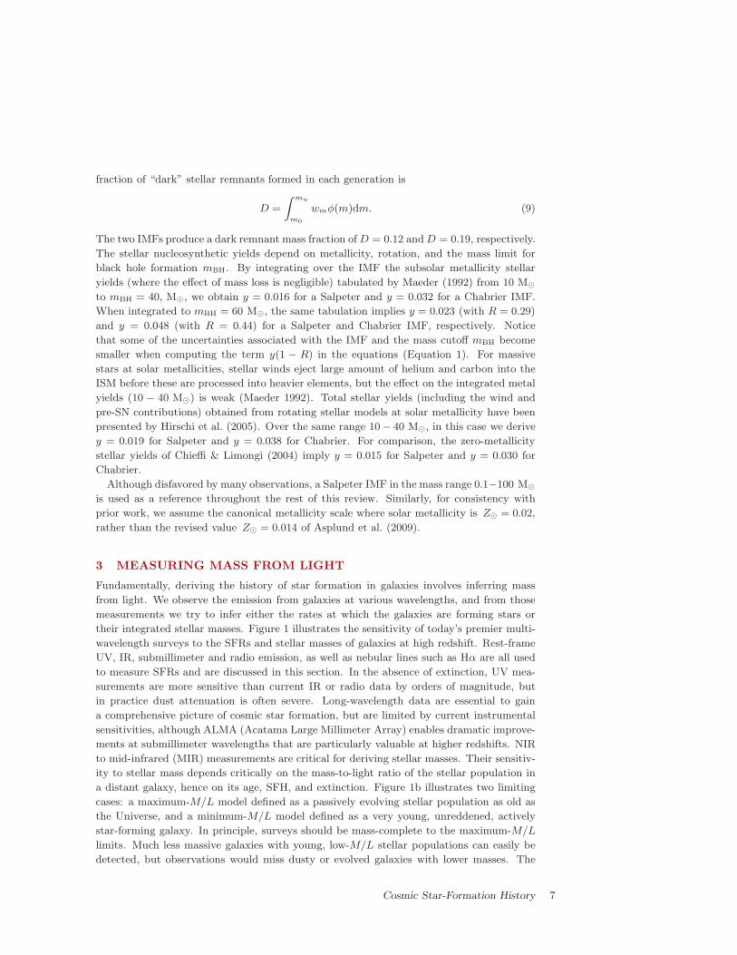
fraction of “dark” stellar remnants formed in each generation is

D =

∫ mu

m0

wmφ(m)dm. (9)

The two IMFs produce a dark remnant mass fraction ofD = 0.12 andD = 0.19, respectively.

The stellar nucleosynthetic yields depend on metallicity, rotation, and the mass limit for

black hole formation mBH. By integrating over the IMF the subsolar metallicity stellar

yields (where the effect of mass loss is negligible) tabulated by Maeder (1992) from 10 M⊙

to mBH = 40, M⊙, we obtain y = 0.016 for a Salpeter and y = 0.032 for a Chabrier IMF.

When integrated to mBH = 60 M⊙, the same tabulation implies y = 0.023 (with R = 0.29)

and y = 0.048 (with R = 0.44) for a Salpeter and Chabrier IMF, respectively. Notice

that some of the uncertainties associated with the IMF and the mass cutoff mBH become

smaller when computing the term y(1 − R) in the equations (Equation 1). For massive

stars at solar metallicities, stellar winds eject large amount of helium and carbon into the

ISM before these are processed into heavier elements, but the effect on the integrated metal

yields (10 − 40 M⊙) is weak (Maeder 1992). Total stellar yields (including the wind and

pre-SN contributions) obtained from rotating stellar models at solar metallicity have been

presented by Hirschi et al. (2005). Over the same range 10− 40 M⊙, in this case we derive

y = 0.019 for Salpeter and y = 0.038 for Chabrier. For comparison, the zero-metallicity

stellar yields of Chieffi & Limongi (2004) imply y = 0.015 for Salpeter and y = 0.030 for

Chabrier.

Although disfavored by many observations, a Salpeter IMF in the mass range 0.1−100 M⊙

is used as a reference throughout the rest of this review. Similarly, for consistency with

prior work, we assume the canonical metallicity scale where solar metallicity is Z⊙ = 0.02,

rather than the revised value Z⊙ = 0.014 of Asplund et al. (2009).

3 MEASURING MASS FROM LIGHT

Fundamentally, deriving the history of star formation in galaxies involves inferring mass

from light. We observe the emission from galaxies at various wavelengths, and from those

measurements we try to infer either the rates at which the galaxies are forming stars or

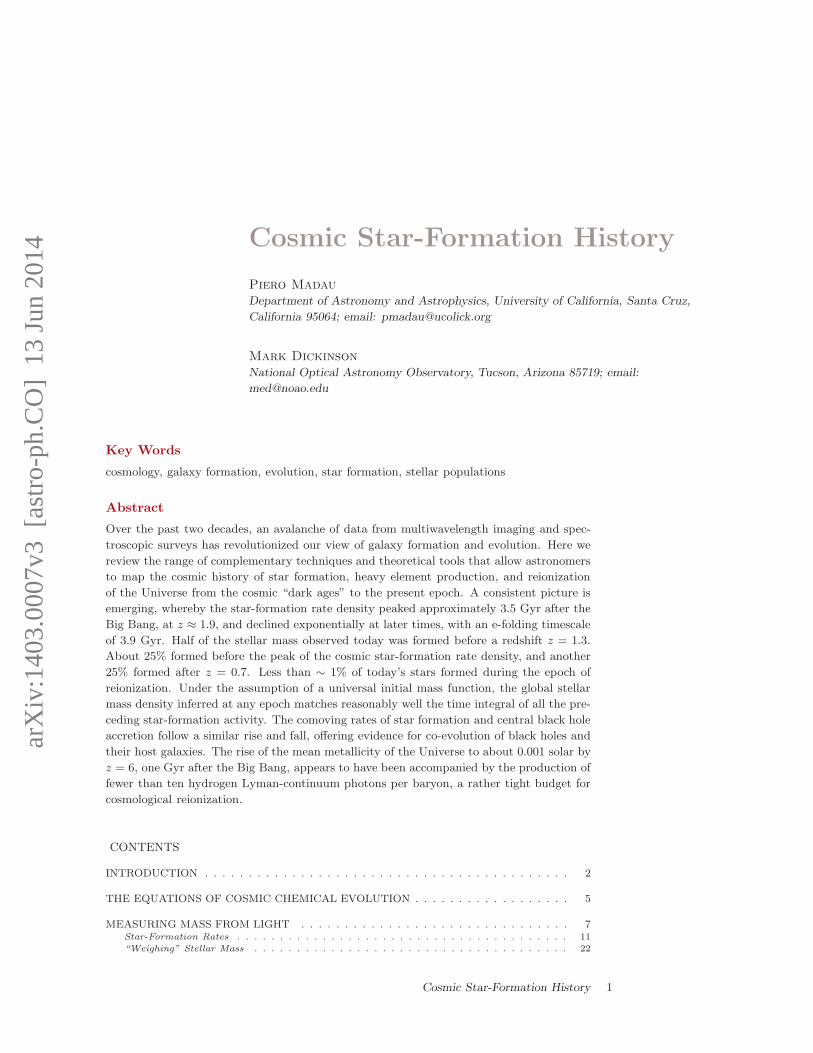
their integrated stellar masses. Figure 1 illustrates the sensitivity of today’s premier multi-

wavelength surveys to the SFRs and stellar masses of galaxies at high redshift. Rest-frame

UV, IR, submillimeter and radio emission, as well as nebular lines such as Hα are all used

to measure SFRs and are discussed in this section. In the absence of extinction, UV mea-

surements are more sensitive than current IR or radio data by orders of magnitude, but

in practice dust attenuation is often severe. Long-wavelength data are essential to gain

a comprehensive picture of cosmic star formation, but are limited by current instrumental

sensitivities, although ALMA (Acatama Large Millimeter Array) enables dramatic improve-

ments at submillimeter wavelengths that are particularly valuable at higher redshifts. NIR

to mid-infrared (MIR) measurements are critical for deriving stellar masses. Their sensitiv-

ity to stellar mass depends critically on the mass-to-light ratio of the stellar population in

a distant galaxy, hence on its age, SFH, and extinction. Figure 1b illustrates two limiting

cases: a maximum-M/L model defined as a passively evolving stellar population as old as

the Universe, and a minimum-M/L model defined as a very young, unreddened, actively

star-forming galaxy. In principle, surveys should be mass-complete to the maximum-M/L

limits. Much less massive galaxies with young, low-M/L stellar populations can easily be

detected, but observations would miss dusty or evolved galaxies with lower masses. The


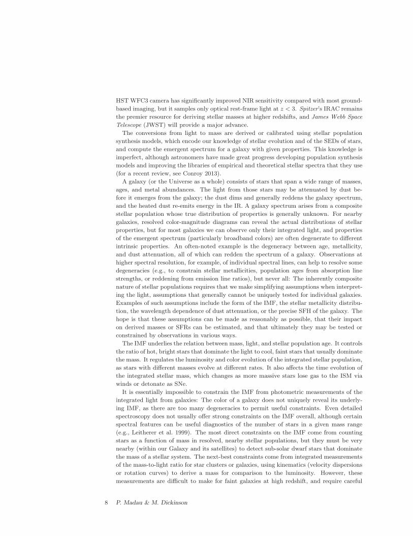
HST WFC3 camera has significantly improved NIR sensitivity compared with most ground-

based imaging, but it samples only optical rest-frame light at z < 3. Spitzer’s IRAC remains

the premier resource for deriving stellar masses at higher redshifts, and James Webb Space

Telescope (JWST) will provide a major advance.

The conversions from light to mass are derived or calibrated using stellar population

synthesis models, which encode our knowledge of stellar evolution and of the SEDs of stars,

and compute the emergent spectrum for a galaxy with given properties. This knowledge is

imperfect, although astronomers have made great progress developing population synthesis

models and improving the libraries of empirical and theoretical stellar spectra that they use

(for a recent review, see Conroy 2013).

A galaxy (or the Universe as a whole) consists of stars that span a wide range of masses,

ages, and metal abundances. The light from those stars may be attenuated by dust be-

fore it emerges from the galaxy; the dust dims and generally reddens the galaxy spectrum,

and the heated dust re-emits energy in the IR. A galaxy spectrum arises from a composite

stellar population whose true distribution of properties is generally unknown. For nearby

galaxies, resolved color-magnitude diagrams can reveal the actual distributions of stellar

properties, but for most galaxies we can observe only their integrated light, and properties

of the emergent spectrum (particularly broadband colors) are often degenerate to different

intrinsic properties. An often-noted example is the degeneracy between age, metallicity,

and dust attenuation, all of which can redden the spectrum of a galaxy. Observations at

higher spectral resolution, for example, of individual spectral lines, can help to resolve some

degeneracies (e.g., to constrain stellar metallicities, population ages from absorption line

strengths, or reddening from emission line ratios), but never all: The inherently composite

nature of stellar populations requires that we make simplifying assumptions when interpret-

ing the light, assumptions that generally cannot be uniquely tested for individual galaxies.

Examples of such assumptions include the form of the IMF, the stellar metallicity distribu-

tion, the wavelength dependence of dust attenuation, or the precise SFH of the galaxy. The

hope is that these assumptions can be made as reasonably as possible, that their impact

on derived masses or SFRs can be estimated, and that ultimately they may be tested or

constrained by observations in various ways.

The IMF underlies the relation between mass, light, and stellar population age. It controls

the ratio of hot, bright stars that dominate the light to cool, faint stars that usually dominate

the mass. It regulates the luminosity and color evolution of the integrated stellar population,

as stars with different masses evolve at different rates. It also affects the time evolution of

the integrated stellar mass, which changes as more massive stars lose gas to the ISM via

winds or detonate as SNe.

It is essentially impossible to constrain the IMF from photometric measurements of the

integrated light from galaxies: The color of a galaxy does not uniquely reveal its underly-

ing IMF, as there are too many degeneracies to permit useful constraints. Even detailed

spectroscopy does not usually offer strong constraints on the IMF overall, although certain

spectral features can be useful diagnostics of the number of stars in a given mass range

(e.g., Leitherer et al. 1999). The most direct constraints on the IMF come from counting

stars as a function of mass in resolved, nearby stellar populations, but they must be very

nearby (within our Galaxy and its satellites) to detect sub-solar dwarf stars that dominate

the mass of a stellar system. The next-best constraints come from integrated measurements

of the mass-to-light ratio for star clusters or galaxies, using kinematics (velocity dispersions

or rotation curves) to derive a mass for comparison to the luminosity. However, these

measurements are difficult to make for faint galaxies at high redshift, and require careful


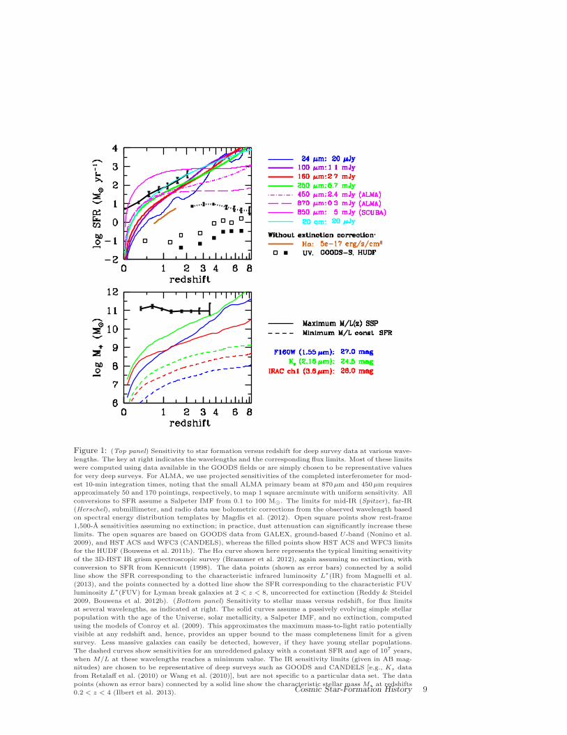
Figure 1: (Top panel) Sensitivity to star formation versus redshift for deep survey data at various wave-

lengths. The key at right indicates the wavelengths and the corresponding flux limits. Most of these limits

were computed using data available in the GOODS fields or are simply chosen to be representative values

for very deep surveys. For ALMA, we use projected sensitivities of the completed interferometer for mod-

est 10-min integration times, noting that the small ALMA primary beam at 870µm and 450µm requires

approximately 50 and 170 pointings, respectively, to map 1 square arcminute with uniform sensitivity. All

conversions to SFR assume a Salpeter IMF from 0.1 to 100 M⊙. The limits for mid-IR (Spitzer), far-IR

(Herschel), submillimeter, and radio data use bolometric corrections from the observed wavelength based

on spectral energy distribution templates by Magdis et al. (2012). Open square points show rest-frame

1,500-A sensitivities assuming no extinction; in practice, dust attenuation can significantly increase these

limits. The open squares are based on GOODS data from GALEX, ground-based U-band (Nonino et al.

2009), and HST ACS and WFC3 (CANDELS), whereas the filled points show HST ACS and WFC3 limits

for the HUDF (Bouwens et al. 2011b). The Hα curve shown here represents the typical limiting sensitivity

of the 3D-HST IR grism spectroscopic survey (Brammer et al. 2012), again assuming no extinction, with

conversion to SFR from Kennicutt (1998). The data points (shown as error bars) connected by a solid

line show the SFR corresponding to the characteristic infrared luminosity L∗(IR) from Magnelli et al.

(2013), and the points connected by a dotted line show the SFR corresponding to the characteristic FUV

luminosity L∗(FUV) for Lyman break galaxies at 2 < z < 8, uncorrected for extinction (Reddy & Steidel

2009, Bouwens et al. 2012b). (Bottom panel) Sensitivity to stellar mass versus redshift, for flux limits

at several wavelengths, as indicated at right. The solid curves assume a passively evolving simple stellar

population with the age of the Universe, solar metallicity, a Salpeter IMF, and no extinction, computed

using the models of Conroy et al. (2009). This approximates the maximum mass-to-light ratio potentially

visible at any redshift and, hence, provides an upper bound to the mass completeness limit for a given

survey. Less massive galaxies can easily be detected, however, if they have young stellar populations.

The dashed curves show sensitivities for an unreddened galaxy with a constant SFR and age of 107 years,

when M/L at these wavelengths reaches a minimum value. The IR sensitivity limits (given in AB mag-

nitudes) are chosen to be representative of deep surveys such as GOODS and CANDELS [e.g., Ks data

from Retzlaff et al. (2010) or Wang et al. (2010)], but are not specific to a particular data set. The data

points (shown as error bars) connected by a solid line show the characteristic stellar mass M∗ at redshifts

0.2 < z < 4 (Ilbert et al. 2013). Cosmic Star-Formation History 9

modeling to account for the role of dark matter and many other effects.

For lack of better information, astronomers often assume that the IMF is universal,

with the same shape at all times and in all galaxies. Although the IMF of various stellar

populations within the Milky Way appears to be invariant (for a review, see Bastian et al.

2010), recent studies suggest that the low-mass IMF slope may be a function of the global

galactic potential, becoming increasingly shallow (bottom-light) with decreasing galaxy

velocity dispersion (Conroy & van Dokkum 2012, Geha et al. 2013). It is still unknown,

however, how galaxy to galaxy variations may affect the “cosmic” volume-averaged IMF as

a function of redshift. In Section 5, we see how a universal IMF can provide a reasonably

consistent picture of the global SFH. The exact shape of the IMF at low stellar masses is

fairly unimportant for deriving relative stellar masses or SFRs for galaxies. Low-mass stars

contribute most of the mass but almost none of the light, and do not evolve over a Hubble

time. Therefore, changing the low-mass IMF mainly rescales the mass-to-light ration M/L

and, hence, affects both stellar masses and SFRs derived from photometry to a similar

degree. Changes to the intermediate- and high-mass region of the IMF, however, can have

significant effects on the luminosity, color evolution, and the galaxy properties derived from

photometry. It is quite common to adopt the simple power-law IMF of Salpeter (1955),

truncated over a finite mass range (generally, 0.1 to 100 M⊙, as adopted in this review).

However, most observations show that the actual IMF turns over from the Salpeter slope

at masses < 1 M⊙, resulting in smaller M/L ratios than those predicted by the Salpeter

IMF. Some common versions of such an IMF are the broken power-law representation used

by Kroupa (2001) and the log-normal turnover suggested by Chabrier (2003).

Dust extinction is another important effect that must often be assumed or inferred,

rather than directly measured. The shape of the extinction law depends on the properties

of the dust grains causing the extinction. For observations of a single star, photons may

be absorbed by dust or scattered out of the observed sightline. However, galaxies are

3D structures with mixed and varying distributions of stars and dust. Photons may be

scattered both into and out of the sightline, and the optical depth of dust along the line of

sight to the observer will be different for every star in the galaxy. These effects are generally

lumped together into the simplifying assumption of a net dust attenuation curve, and such

relations have been derived for local galaxy samples both empirically (e.g., Calzetti et al.

2000) and using theoretical modeling (Charlot & Fall 2000). However, all galaxies are not

equal, and no net attenuation law is equally appropriate for all galaxies. There can always

be stars that are completely obscured behind optically thick dust such that little or none of

their light emerges directly from the galaxy, except re-radiated as dust emission. Although

this may not be a significant factor for many galaxies, there are certainly some starburst

galaxies in which huge and bolometrically dominant star-formation activity takes place in

regions screened by hundreds of magnitudes of dust extinction. UV/optical measurements

will never detect this light, but the star formation can be detected and measured at other

wavelengths, e.g., with FIR or radio data.

In order to derive SFRs or stellar masses for galaxies using stellar population synthesis

models, astronomers typically assume relatively simple, parameterized SFHs. However, the

SFHs of individual galaxies are unlikely to be smooth and simple; they may vary on both

long and short timescales. The fact that young stars are more luminous than older stars

leads to the problem of “outshining” (e.g., Papovich et al. 2001, Maraston et al. 2010) – the

light from older stars can be lost in the glare of more recent star formation and contributes

relatively little to the observed photometry from a galaxy, even if those stars contribute

significantly to its mass. SED model fits to galaxies with recent star formation tend to be


driven largely by the younger, brighter starlight, and may not constrain the mass (or other

properties) of older stars that may be present.

For the Universe as a whole there is one “cosmic” IMF that represents the global average

at a given time or redshift, regardless of whether the IMF varies from one galaxy to another.

Similarly, there is a “cosmic” distribution of metallicities, a “cosmic” net attenuation of

starlight by dust at a given wavelength, and the Universe as a whole obeys one “cosmic”

SFH that, moreover, was probably relatively smooth over time – i.e., any stochasticity or

“burstiness” averages out when considered for the Universe as a whole. In principle, these

facts can simplify the determination of the cosmic SFH, particularly when it is derived

from measurements of integrated light averaging over all galaxies. In practice, however,

astronomers often derive SFRs and stellar masses for individual galaxies in their deep

surveys, and then sum them to derive comoving volume averages. In which case, some

of the advantages of the “cosmic averaging” are reduced.

3.1 Star-Formation Rates

There are many ways in which to infer SFRs from observations of the integrated light from

galaxies. Kennicutt (1998) and Kennicutt & Evans (2012) have presented extensive reviews

of this topic, and here we recap only points that are especially relevant for measurements

of the global SFH, particularly at high redshift. Virtually all observational tracers of star

formation fundamentally measure the rate of massive star formation, because massive stars

emit most of the energy from a young stellar population. However, different observational

tracers are sensitive to different ranges of stellar masses: hence, they respond differently

as a function of stellar population age. For example, Hα emission arises primarily from

HII regions photoionized by O stars with lifetimes shorter than 20 Myr, whereas the UV

continuum is produced by stars with a broader mass range and with longer lifetimes. The

time-dependence of different indicators can complicate efforts to derive accurate SFRs for

individual galaxies, especially if their SFRs may be rapidly changing (e.g., during a starburst

event), but they should average out when summing over a whole population of galaxies.

3.1.1 UV light Newly-formed stellar populations emit radiation over a broad spec-

trum. For a normal IMF, low-mass stars dominate the mass integrated over the whole

stellar population, but at young ages the luminosity is dominated by ultraviolet emission

from massive stars. These stars have short lifetimes, so the UV emission fades quickly. For

a Salpeter IMF, the 1,500-A luminosity from an evolving simple stellar population (SSP)

(i.e., an ensemble of stars formed instantaneously and evolving together) with solar metal-

licity fades by a factor of 100 after 108 years, and by factors of 103 to 106 after 109 years,

depending on metallicity (Figure 2). Bolometrically, at least half of the luminous energy

that an SSP produces over a 10-Gyr cosmic lifetime emerges in the first 100 Myr, mostly

in the UV, making this a natural wavelength from which to infer SFRs.

For a galaxy forming stars at a constant rate, the 1,500-A luminosity stabilizes once O-

stars start to evolve off the main sequence. For solar metallicity, by an age of 107.5 years,

the 1,500-A luminosity has reached 75% of its asymptotic value, although convergence is

somewhat slower at lower metallicity (Figure 2). For these reasons, the UV luminosity

at wavelengths of ∼ 1,500 A (wavelengths from 1400 A to 1700 A have been used in the

literature for both local and high redshift studies) is regarded as a good tracer of the

formation rate of massive stars, provided that the timescale for significant fluctuations in

the SFR is longer than a few 107 years. For shorter bursts or dips in the SFR, changes in


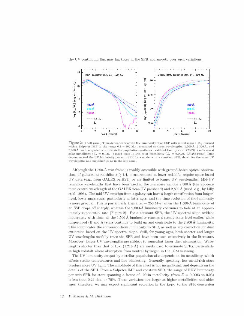
the UV continuum flux may lag those in the SFR and smooth over such variations.

Figure 2: (Left panel) Time dependence of the UV luminosity of an SSP with initial mass 1 M⊙, formed

with a Salpeter IMF in the range 0.1 − 100 M⊙, measured at three wavelengths, 1,500 A, 2,300 A, and

2,800 A, and computed with the stellar population synthesis models of Conroy et al. (2009): (solid lines)

solar metallicity (Z∗ = 0.02), (dashed lines 1/10th solar metallicity (Z∗ = 0.002). (Right panel) Time

dependence of the UV luminosity per unit SFR for a model with a constant SFR, shown for the same UV

wavelengths and metallicities as in the left panel.

Although the 1,500-A rest frame is readily accessible with ground-based optical observa-

tions of galaxies at redshifts z & 1.4, measurements at lower redshifts require space-based

UV data (e.g., from GALEX or HST) or are limited to longer UV wavelengths. Mid-UV

reference wavelengths that have been used in the literature include 2,300 A (the approxi-

mate central wavelength of the GALEX near-UV passband) and 2,800 A (used, e.g., by Lilly

et al. 1996). The mid-UV emission from a galaxy can have a larger contribution from longer-

lived, lower-mass stars, particularly at later ages, and the time evolution of the luminosity

is more gradual. This is particularly true after ∼ 250 Myr, when the 1,500-A luminosity of

an SSP drops off sharply, whereas the 2,800-A luminosity continues to fade at an approx-

imately exponential rate (Figure 2). For a constant SFR, the UV spectral slope reddens

moderately with time, as the 1,500 A luminosity reaches a steady-state level earlier, while

longer-lived (B and A) stars continue to build up and contribute to the 2,800 A luminosity.

This complicates the conversion from luminosity to SFR, as well as any correction for dust

extinction based on the UV spectral slope. Still, for young ages, both shorter and longer

UV wavelengths usefully trace the SFR and have been used extensively in the literature.

Moreover, longer UV wavelengths are subject to somewhat lesser dust attenuation. Wave-

lengths shorter than that of Lyα (1,216 A) are rarely used to estimate SFRs, particularly

at high redshift where absorption from neutral hydrogen in the IGM is strong.

The UV luminosity output by a stellar population also depends on its metallicity, which

affects stellar temperatures and line blanketing. Generally speaking, less-metal-rich stars

produce more UV light. The amplitude of this effect is not insignificant, and depends on the

details of the SFH. From a Salpeter IMF and constant SFR, the range of FUV luminosity

per unit SFR for stars spanning a factor of 100 in metallicity (from Z = 0.0003 to 0.03)

is less than 0.24 dex, or 70%. These variations are larger at higher metallicities and older

ages; therefore, we may expect significant evolution in the LFUV to the SFR conversion


factor as the global metallicity of galaxies evolves.

We express the conversion factor between the intrinsic FUV-specific luminosity Lν(FUV)

(before extinction, or corrected for extinction) and the ongoing SFR as

SFR = KFUV × Lν(FUV), (10)

where Lν(FUV) is expressed in units of erg s−1 Hz−1 and SFR in units of M⊙ year−1.

The precise value of the conversion factor KFUV is sensitive to the recent SFH and metal-

enrichment history as well as to the choice of the IMF. It is relatively insensitive to the

exact FUV wavelength, as the UV spectrum of a galaxy with a constant SFR is quite

flat in fν units, at least for ages much longer than 107 years. Generally in this re-

view, we use FUV to refer to 1,500-A emission or are explicit when we refer to other

UV wavelengths. For a Salpeter IMF in the mass range 0.1 − 100 M⊙ and constant

SFR, the flexible stellar population synthesis (FSPS) models of Conroy et al. (2009) yield

KFUV = (1.55, 1.3, 1.1, 1.0)×10−28 for logZ∗/Z⊙ = (+0.2, 0,−0.5,−1.0) at age ∼> 300 Myr.

The GALAXEV models of Bruzual & Charlot (2003) yield values of KFUV that are ∼5%

smaller.

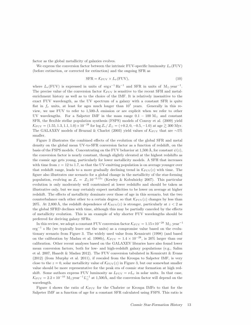
Figure 3 illustrates the combined effects of the evolution of the global SFR and metal

density on the global mean UV-to-SFR conversion factor as a function of redshift, on the

basis of the FSPS models. Concentrating on the FUV behavior at 1,500 A, for constant ψ(z),

the conversion factor is nearly constant, though slightly elevated at the highest redshifts as

the cosmic age gets young, particularly for lower metallicity models. A SFH that increases

with time from z = 12 to 1.7, so that the UV-emitting population is on average younger over

that redshift range, leads to a more gradually declining trend in KFUV(z) with time. The

figure also illustrates one scenario for a global change in the metallicity of the star-forming

population, evolving as Z∗ = Z⊙10−0.15z (Kewley & Kobulnicky 2007). This particular

evolution is only moderately well constrained at lower redshifts and should be taken as

illustrative only, but we may certainly expect metallicities to be lower on average at higher

redshift. The effects of metallicity dominate over those of age in this scenario, but the two

counterbalance each other other to a certain degree, so that KFUV(z) changes by less than

20%. At 2,800 A, the redshift dependence of KNUV(z) is stronger, particularly at z < 2 as

the global SFRD declines with time, although this may be partially canceled by the effects

of metallicity evolution. This is an example of why shorter FUV wavelengths should be

preferred for deriving galaxy SFRs.

In this review, we adopt a constant FUV conversion factor KFUV = 1.15×10−28 M⊙ year−1

erg−1 s Hz (we typically leave out the units) as a compromise value based on the evolu-

tionary scenario from Figure 3. The widely used value from Kennicutt (1998) (and based

on the calibration by Madau et al. 1998b), KFUV = 1.4 × 10−28, is 20% larger than our

calibration. Other recent analyses based on the GALAXEV libraries have also found lower

mean conversion factors, both for low- and high-redshift galaxy populations (e.g., Salim

et al. 2007, Haardt & Madau 2012). The FUV conversion tabulated in Kennicutt & Evans

(2012) (from Murphy et al. 2011), if rescaled from the Kroupa to Salpeter IMF, is very

close to the z = 0, solar metallicity value of KFUV(z) in Figure 3, but our somewhat smaller

value should be more representative for the peak era of cosmic star formation at high red-

shift. Some authors express FUV luminosity as LFUV = νLν in solar units. In that case,

KFUV = 2.2×10−10 M⊙year−1L−1

⊙ at 1,500A, and the conversion factor will depend on the

wavelength.

Figure 4 shows the ratio of KFUV for the Chabrier or Kroupa IMFs to that for the

Salpeter IMF as a function of age for a constant SFR calculated using FSPS. This ratio is


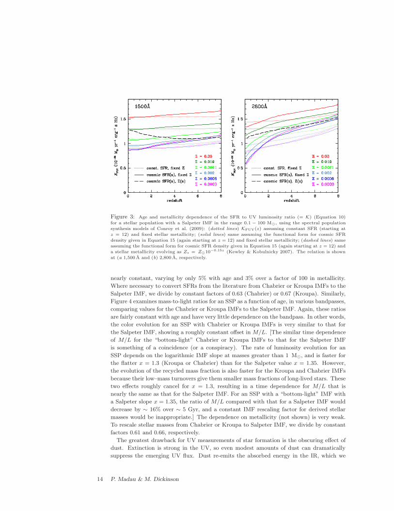
Figure 3: Age and metallicity dependence of the SFR to UV luminosity ratio (= K) (Equation 10)

for a stellar population with a Salpeter IMF in the range 0.1 − 100 M⊙, using the spectral population

synthesis models of Conroy et al. (2009): (dotted lines) KFUV(z) assuming constant SFR (starting at

z = 12) and fixed stellar metallicity; (solid lines) same assuming the functional form for cosmic SFR

density given in Equation 15 (again starting at z = 12) and fixed stellar metallicity; (dashed lines) same

assuming the functional form for cosmic SFR density given in Equation 15 (again starting at z = 12) and

a stellar metallicity evolving as Z∗ = Z⊙10−0.15z (Kewley & Kobulnicky 2007). The relation is shown

at (a 1,500 A and (b) 2,800 A, respectively.

nearly constant, varying by only 5% with age and 3% over a factor of 100 in metallicity.

Where necessary to convert SFRs from the literature from Chabrier or Kroupa IMFs to the

Salpeter IMF, we divide by constant factors of 0.63 (Chabrier) or 0.67 (Kroupa). Similarly,

Figure 4 examines mass-to-light ratios for an SSP as a function of age, in various bandpasses,

comparing values for the Chabrier or Kroupa IMFs to the Salpeter IMF. Again, these ratios

are fairly constant with age and have very little dependence on the bandpass. In other words,

the color evolution for an SSP with Chabrier or Kroupa IMFs is very similar to that for

the Salpeter IMF, showing a roughly constant offset in M/L. [The similar time dependence

of M/L for the “bottom-light” Chabrier or Kroupa IMFs to that for the Salpeter IMF

is something of a coincidence (or a conspiracy). The rate of luminosity evolution for an

SSP depends on the logarithmic IMF slope at masses greater than 1 M⊙, and is faster for

the flatter x = 1.3 (Kroupa or Chabrier) than for the Salpeter value x = 1.35. However,

the evolution of the recycled mass fraction is also faster for the Kroupa and Chabrier IMFs

because their low–mass turnovers give them smaller mass fractions of long-lived stars. These

two effects roughly cancel for x = 1.3, resulting in a time dependence for M/L that is

nearly the same as that for the Salpeter IMF. For an SSP with a “bottom-light” IMF with

a Salpeter slope x = 1.35, the ratio of M/L compared with that for a Salpeter IMF would

decrease by ∼ 16% over ∼ 5 Gyr, and a constant IMF rescaling factor for derived stellar

masses would be inappropriate.] The dependence on metallicity (not shown) is very weak.

To rescale stellar masses from Chabrier or Kroupa to Salpeter IMF, we divide by constant

factors 0.61 and 0.66, respectively.

The greatest drawback for UV measurements of star formation is the obscuring effect of

dust. Extinction is strong in the UV, so even modest amounts of dust can dramatically

suppress the emerging UV flux. Dust re-emits the absorbed energy in the IR, which we


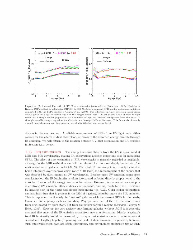
Figure 4: (Left panel) The ratio of SFR/LFUV conversion factors KFUV (Equation 10) for Chabrier or

Kroupa IMFs to that for a Salpeter IMF (0.1 to 100 M⊙), for a constant SFR and for various metallicities,

computed with the FSPS models of Conroy et al. (2009). The difference in this conversion factor varies

only slightly with age or metallicity over the ranges shown here. (Right panel) Ratio of mass-to-light

ratios for a simple stellar population as a function of age, for various bandpasses from the near-UV

through near-IR, comparing values for Chabrier and Kroupa IMFs to Salpeter. This factor also has only

a small dependence on age, bandpass, or metallicity (the last not shown here).

discuss in the next section. A reliable measurement of SFRs from UV light must either

correct for the effects of dust absorption, or measure the absorbed energy directly through

IR emission. We will return to the relation between UV dust attenuation and IR emission

in Section 3.1.3 below.

3.1.2 Infrared emission The energy that dust absorbs from the UV is re-radiated at

MIR and FIR wavelengths, making IR observations another important tool for measuring

SFRs. The effect of dust extinction at FIR wavelengths is generally regarded as negligible,

although in the MIR extinction can still be relevant for the most deeply buried star for-

mation and active galactic nuclei (AGN). The total IR luminosity (LIR, usually defined as

being integrated over the wavelength range 8–1000 µm) is a measurement of the energy that

was absorbed by dust, mainly at UV wavelengths. Because most UV emission comes from

star formation, the IR luminosity is often interpreted as being directly proportional to the

absorbed fraction of the energy from star formation. However, active nuclei can also pro-

duce strong UV emission, often in dusty environments, and may contribute to IR emission

by heating dust in the torus and clouds surrounding the AGN. Older stellar populations

can also heat dust that is present in the ISM of a galaxy, contributing to the FIR emission.

This is important particularly for “mature” galaxies with low current SFRs in the nearby

Universe: For a galaxy such as our Milky Way, perhaps half of the FIR emission comes

from dust heated by older stars, not from young star-forming regions (Lonsdale Persson &

Helou 1987). However, for very actively star-forming galaxies without AGN it is generally

assumed that most of the IR emission arises from new star formation. Ideally, a galaxy’s

total IR luminosity would be measured by fitting a dust emission model to observations at

several wavelengths, hopefully spanning the peak of dust emission. In practice, however,

such multiwavelength data are often unavailable, and astronomers frequently use an SED


template that is often derived from observations of local galaxies to extrapolate from a

single observed flux density at some MIR or FIR wavelength, not necessarily close to the

dust emission peak, to a total LIR. Thus, variations in the dust emission properties from

galaxy to galaxy can lead to significant uncertainties in not only this bolometric correction,

but also in the estimation of SFRs.

Arising from various components heated to different temperatures, the spectrum of dust

emission is fairly complex. Most of the dust mass in a galaxy is usually in the form of rela-

tively cold dust (15-60 K) that contributes strongly to the emission at FIR and submillimeter

wavelengths (30-1,000 µm). Dust at several different temperatures may be present, including

both colder grains in the ambient ISM and warmer grains in star-forming regions. Emission

from still hotter, small-grain dust in star-forming regions, usually transiently heated by sin-

gle photons and not in thermal equilibrium, can dominate the MIR continuum (λ < 30µm)

and may serve as a useful SFR indicator (e.g., Calzetti et al. 2007). The MIR spectral

region (3–20µm) is both spectrally and physically complex: It has strong emission bands

from polycyclic aromatic hydrocarbons and absorption bands primarily from silicates. The

strength of emission from polycyclic aromatic hydrocarbons can depend strongly on ISM

metallicity and radiation field intensity (e.g., Engelbracht et al. 2005, 2008, Smith et al.

2007). Strong silicate absorption features are seen when the column density of dust and

gas is particularly large toward obscured AGN and perhaps even nuclear starburst regions.

AGN may contribute strong continuum emission from warm dust, and can dominate over

star formation at MIR wavelengths. By contrast, in the FIR, their role is less prominent.

The Infrared Space Observatory (ISO) and the Spitzer Space Telescope were the first

telescopes with MIR sensitivities sufficient to detect galaxies at cosmological redshifts. In

particular, Spitzer observations at 24µm with the MIPS instrument are very sensitive and

capable of detecting “normal” star-forming galaxies out to z ≈ 2 in modest integration

times. Spitzer is also very efficient for mapping large sky areas. It has a 24-µm beam

size that is small enough (5.7 arcsec) to reliably identify faint galaxy counterparts to the

IR emission. However, only a fraction of the total IR luminosity emerges in the MIR. As

noted above, it is a complicated spectral region that leads to large and potentially quite

uncertain bolometric corrections from the observed MIR flux to the total IR luminosity. At

z ≈ 2, where 24-µm observations sample rest-frame wavelengths around 8µm, where the

strongest polycyclic aromatic hydrocarbon bands are found, spectral templates based on

local galaxies span more than an order of magnitude in the ratio LIR/L8µm (e.g., Chary

& Elbaz 2001, Dale & Helou 2002, Dale et al. 2005). More information about the type

of galaxy being observed is needed to choose with confidence an appropriate template to

convert the observed MIR luminosity to LIR or a SFR.

The FIR thermal emission is a simpler and more direct measurement of star-formation

energy. Partly owing to their large beam sizes that resulted in significant confusion and

blending of sources and in difficulty localizing galaxy counterparts, ISO and Spitzer offer

only relatively limited FIR sensitivity for deep observations. The Herschel Space Observa-

tory dramatically improved such observations: Its 3.5-m mirror diameter provided a point

spread function FWHM (full width half maximum) small enough to minimize confusion

and to identify source counterparts in observations from 70 to 250µm. However, at the

longest wavelengths of the Herschel SPIRE instrument, 350 and 500µm, confusion becomes

severe. Herschel observations can directly detect galaxies near the peak of their FIR dust

emission: Dust SEDs typically peak at 60-100µm in the rest frame, within the range of

Herschel observations out to z < 4. Temperature variations in galaxies lead to variations

in the bolometric corrections for observations at a single wavelength, but these differences


are much smaller than for MIR data, generally less then factors of 2.

Despite Herschel’s FIR sensitivity, deep Spitzer 24-µm observations, in general, still detect

more high-z sources down to lower limiting IR luminosities or SFRs. At z ≈ 2, the deepest

Herschel observations only barely reach to roughly L∗IR [the characteristic luminosity of the

“knee” of the IR luminosity function (IRLF)], leaving a large fraction of the total cosmic

SFRD undetected, at least for individual sources, although stacking can be used to probe

to fainter levels. Deep Spitzer 24-µm observations detect galaxies with SFRs several times

lower, and many fields were surveyed to faint limiting fluxes at 24-µm during Spitzer’s

cryogenic lifetime. Therefore, there is still value in trying to understand and calibrate ways

to measure star formation from deep MIR data, despite the large and potentially uncertain

bolometric corrections.

In practice, observations of IR-luminous galaxies detected at high redshift with both

Spitzer and Herschel have demonstrated that the IR SEDs for many galaxies are well-

behaved and that variations can be understood at least in part. Several pre-Herschel studies

(Papovich et al. 2007, Daddi et al. 2007, Magnelli et al. 2009, 2011) compared 24-µm

observations of distant galaxies with those of other SFR tracers, including Spitzer FIR

measurements (either individual detections or stacked averages) and radio emission. On

average, the MIR to FIR flux ratios for galaxies at z . 1.3 match those predicted by local

IR SED templates such as those of Chary & Elbaz (2001), implying that 24-µm-derived

SFRs should be reliable. However, at higher redshift, 1.3 < z < 2.5, the 24-µm fluxes were

brighter than expected relative to the FIR or radio data, i.e., SFRs derived from 24-µm data

using local SED templates may be systematically overestimated at z ≈ 2. This result was

upheld by early Herschel studies (Nordon et al. 2010, Elbaz et al. 2010). In a joint analysis

of the IR SED properties of both nearby and high-redshift IR-luminous galaxies, Elbaz et al.

(2011) provided an explanatory framework for these observations in terms of the distinction

between a majority population of galaxies obeying a “main-sequence” correlation between

their SFRs and stellar masses and a minority “starburst” population with substantially

higher SFRs per unit mass (or sSFR). Locally, starburst galaxies have more compact, high

surface density star forming regions, whereas normal disk galaxies on the star-forming

main sequence have star formation distributed on larger scales with lower surface density.

Starbursts also have warmer average dust temperatures and a significantly larger ratio

between their FIR and 8-µm rest-frame luminosities than those of the main-sequence disk

galaxies. Locally, most luminous and ultraluminous IR galaxies (LIRGs and ULIRGs, with

LIR > 1011L⊙ and > 1012L⊙, respectively) are merger-driven starbursts, but at z ≈ 2

where the SFRs and sSFRs of galaxies are globally much larger, the majority of LIRGs and

ULIRGs are “normal” main-sequence galaxies. Their IR SEDs are more similar to those of

ordinary, local star-forming spiral galaxies, and have smaller bolometric corrections from

observed 24-µm data (rest frame λ ≈ 8µm) than those predicted by SED templates designed

to match local LIRGs and ULIRGs. Elbaz et al. (2011) constructed a “universal” main-

sequence SED from the ensemble of high-z Spitzer and Herschel photometry for galaxies

in the Great Observatories Origins Deep Survey (GOODS) fields at 0.3 < z < 2.5. This

SED leads to consistent total IR luminosities for the large majority of galaxies over that

redshift range. Although no single template can be used to accurately derive LIR or SFR

from MIR observations for all galaxies, we now have a better understanding of how this can

be done on average, which may be sufficient for deriving the global redshift evolution of the

IR luminosity density or its corresponding SFRD. Rodighiero et al. (2011) (see also Sargent

et al. 2012) showed that starbursts (whose IR SEDs deviate significantly from those of the

main-sequence population) account for only 10% of the global SFRD at z ≈ 2. With the


data now available from Herschel and Spitzer, a broad understanding of the evolving IRLF

and IR luminosity density, at least at 0 < z < 2.5, seems within reach.

MIR and FIR observations require space-based telescopes, but at submillimeter and mil-

limeter wavelengths, observations can once again be made from the ground within certain

atmospheric transmission windows. The advent of submillimeter bolometer array cameras

such as SCUBA on the JCMT revolutionized the field, and led to the first detections of a

large population of ULIRGs at high redshift (e.g., Smail et al. 1997, Hughes et al. 1998,

Barger et al. 1998). Until recently, only the most luminous high-z objects could be readily

detected, but the new ALMA interferometer will improve detection sensitivities by more

than an order of magnitude, albeit over small fields of view. As noted above, submillimeter

observations measure emission beyond the peak of dust emission, where flux is declining

steeply with wavelength in the Rayleigh-Jeans part of the SED. This leads to a negative

K correction so strong that it cancels out the effects of distance: A galaxy with a given

IR luminosity will have roughly constant submillimeter flux if it is observed at any red-

shift 1 < z < 10. By contrast, the bolometric corrections from the observed submillimeter

wavelengths to the total IR luminosities are large and depend strongly on dust temperature.

This can lead to significant uncertainties interpreting submillimeter fluxes from high-redshift

sources, and a bias toward detecting galaxies with the coldest dust emission.

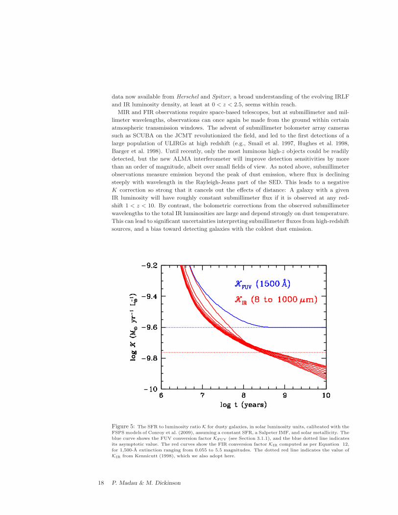
Figure 5: The SFR to luminosity ratio K for dusty galaxies, in solar luminosity units, calibrated with the

FSPS models of Conroy et al. (2009), assuming a constant SFR, a Salpeter IMF, and solar metallicity. The

blue curve shows the FUV conversion factor KFUV (see Section 3.1.1), and the blue dotted line indicates

its asymptotic value. The red curves show the FIR conversion factor KIR computed as per Equation 12,

for 1,500-A extinction ranging from 0.055 to 5.5 magnitudes. The dotted red line indicates the value of

KIR from Kennicutt (1998), which we also adopt here.


By analogy with Equation 10, we express the conversion from IR luminosity (LIR) to

ongoing SFR as

SFRIR = KIR × LIR, (11)

where LIR is the IR luminosity integrated over the wavelength range from 8 to 1,000µm.

Here, it is assumed that the IR emission is entirely due to recent star formation, but in

practice, AGN and older stars can contribute to dust heating. Furthermore, if the net dust

opacity to young star-forming regions in a galaxy is not large, and if a significant amount of

UV radiation emerges, then the SFR derived from the IR luminosity will represent only a

fraction of the total. Hence, we write SFRIR in Equation 11 to indicate that this is only the

dust-obscured component of the SFR. For this reason, some authors advocate summing the

SFRs derived from the observed IR and UV luminosity densities, the latter uncorrected for

extinction. Once again, we calibrate the conversion factor KIR using the FSPS models of

Conroy et al. (2009), which also incorporate dust attenuation and re-emission. We assume

simple foreground-screen dust attenuation from Calzetti et al. (2000), although the details

of the dust absorption model matter relatively little. The luminosity integrated from 8

to 1000 µm depends only mildly on the detailed dust emission parameters (essentially, the

dust temperature distribution) for a broad range of reasonable values. Because the dust

luminosity is primarily reprocessed UV emission from young star formation, the conversion

factor KIR also depends on the details of the SFH and on metallicity. In practice, we may

expect that galaxies with substantial extinction and bolometrically dominant dust emission

are unlikely to have low metallicities; here we assume solar metallicity for our calibration.

We modify Equation 11 to account for both the FUV and FIR components of star formation:

SFRtot = KFUVLFUV +KIRLIR, (12)

where LFUV is the observed FUV luminosity at 1,500 Awith no correction for extinction.

We use FSPS models with a Salpeter IMF, solar metallicity, and constant SFR to compute

LFUV and LIR as a function of age for various levels of dust attenuation: we then solve for

KIR. Figure 5 shows the result of this calculation: SFR is expressed in units of M⊙ year−1,

and both the FUV and IR luminosities are expressed in solar units (with LFUV = νLν) to

display both on the same scale. As shown in Section 3.1.1, the FUV emission reaches a

steady state after ∼ 300 Myr, and for this calculation, we use the asymptotic value KFUV =

2.5 × 10−10 M⊙ year−1L−1⊙ (equivalently, KFUV = 1.3 × 10−28 M⊙ year−1 erg−1 s Hz).

Instead, LIR increases slowly (hence, KIR decreases) as the optical rest-frame luminosity

of longer-lived stars continues to build, some fraction of which is then absorbed by dust

and re-emitted. This model with constant SFR and constant dust attenuation results in a

modest effect of ∼ 0.1 dex in logKIR per dex in log t. However, in practice, older stars will

likely have lower dust extinction than younger stars, thus further reducing this trend. At

ages of a few 108 years, KIR depends very little on the total extinction. Kennicutt (1998)

proposed a calibration factor KIR = 1.73 × 10−10 M⊙ year−1L−1⊙ , which is fully consistent

with the models shown in Figure 5 for an age of 300 Myr. We adopt that value for this

review. For luminosities measured in cgs units, we can write KIR = 4.5× 10−44 M⊙ year−1

erg−1 s.

3.1.3 UV extinction and IR emission As noted above, dust can substantially atten-

uate UV emission, not only compromising its utility for measuring SFRs, but also producing

IR emission, which is a valuable tracer of star-formation activity. Considerable effort has

been invested in understanding the physics and phenomenology of extinction in galaxies


(for a review, see Calzetti 2001). In principle, the best way to account for the effect of dust

attenuation is to directly measure the energy emitted at both UV and IR wavelengths, i.e.,

both the luminosity that escapes the galaxy directly and that which is absorbed and re-

radiated by dust. This provides a “bolometric” approach to measuring SFRs. In practice,

however, data sensitive enough to measure FIR luminosities of high-redshift galaxies are

often unavailable. Herschel greatly advanced these sorts of observations, but its sensitivity,

although impressive, was sufficient to detect only galaxies with high SFRs > 100 M⊙ yr−1,

at z > 2.

For star-forming galaxies with moderate extinction at z > 1, optical photometry mea-

suring rest-frame UV light is obtained much more easily than are suitably deep FIR, sub-

millimeter or radio data. Current observations of UV light are also typically much more

sensitive to star formation than are those at other wavelengths (Figure 1). As a result,

trying to infer SFRs from rest-frame UV observations alone it tempting, but this requires re-

liable estimates of dust extinction corrections. For example, Lyman break galaxies (LBGs)

are a UV-selected population of star-forming high-redshift galaxies. Their selection would

favor relatively low extinction, but even LBGs are quite dusty: Reddy et al. (2012) used

Herschel observations to determine that, on average, 80% of the FUV emission from typical

(∼ L∗FUV) LBGs at z ≈ 2 is absorbed by dust and re-radiated in the FIR. Many more

massive galaxies with high SFRs have greater extinction. So-called dust-obscured galaxies

(Dey et al. 2008) have MIR to UV flux density ratios > 1, 000 (typically corresponding to

LIR/LFUV > 100) (Penner et al. 2012) and are quite common, contributing 5–10% of the

SFRD at z ≈ 2 (Pope et al. 2008); many of these are nearly or entirely invisible in deep

optical images.

Nevertheless, the widespread availability of rest-frame UV data for high-redshift galaxies

encourages their use for measuring the cosmic SFH. Presently, at z ≫ 2, there is little

alternative: Even the deepest Spitzer, Herschel, radio, or submillimeter surveys can detect

only the rarest and most ultraluminous galaxies at such redshifts. By contrast, deep optical

and NIR surveys have now identified samples of thousands of UV-selected star-forming

galaxies out to z ≈ 7 and beyond.

Attempts to measure and correct for dust extinction in high-z galaxies have generally

used the ultraviolet spectral slope (designated β) as a measure of UV reddening, and have

adopted empirical correlations between UV reddening and UV extinction. Calzetti et al.

(1994, 2000) used ultraviolet and optical spectroscopy to derive an empirical, average dust

attenuation curve for a sample of local UV-bright star-forming galaxies. Meurer et al. (1999)

(later updated by Overzier et al. 2011) used UV and FIR data for a similar local sample

to empirically calibrate the relation between UV reddening (β) and UV extinction (IRX ≡

LIR/LFUV, which can be directly related to AFUV). The reasonably tight IRX–β relation

obeyed by the local UV-bright galaxies is broadly consistent with the Calzetti attenuation

law, hence reinforcing its popularity. However, other local studies showed clearly that some

galaxies deviate from these relations. Goldader et al. (2002) found that nearby ULIRGs

deviate strongly from the Meurer IRX–β relation; these ULIRGs have very large values of

IRX but often with relatively blue UV spectral index β. This was interpreted to mean that

that the observed UV light from local ULIRGs is relatively unreddened star formation in the

host galaxy that is unrelated to the bolometrically dominant star formation, which is entirely

obscured from view at UV-optical wavelengths, and detected only in the FIR. Instead,

observations of ordinary spiral galaxies (Kong et al. 2004, Buat et al. 2005) measured

redder values of β for a given IRX. This is generally taken as evidence that light from older

and less massive stars contributes significantly to the near-UV emission, leading to redder


UV colors for reasons unrelated to extinction. In general, different relative distributions of

stars and dust can lead to different net attenuation properties. Extinction can easily be

patchy: Winds from star-forming regions can blow away dust on certain timescales, whereas

other regions that are younger or more deeply embedded in the galaxy’s ISM remain more

heavily obscured. Dust heating also depends on geometry, leading to different distributions

of dust temperatures and different emission spectra at IR and submillimeter wavelengths.

At high redshift there are only relatively limited tests of the relation between UV red-

dening and extinction. Reddy et al. (2004, 2006, 2010, 2012) have compared various SFR

tracers (including radio, Spitzer 24-µm, and Herschel 100–160-µm emission) to show that

Calzetti/Meurer UV extinction laws are broadly appropriate for the majority of L∗ LBGs

at z ≈ 2. However, they found evidence for systematic deviations for galaxies with the

largest SFRs (> 100 M⊙ year−1), which, similar to local ULIRGs, show “grayer” effective

attenuation (i.e., less UV reddening for their net UV extinction). They also found evidence

for systematic deviations for the youngest galaxies, which show stronger reddening for their

net FUV extinction, perhaps because of the metallicity or geometric effects that steepen

the wavelength dependence of the UV reddening function compared with results from the

Calzetti law. Assuming Calzetti attenuation, Daddi et al. (2007) and Magdis et al. (2010)

also found broad consistency between UV-based and IR- or radio-based SFR measurements

for samples at z ≈ 2–3 (although, see Carilli et al. 2008). However, studies that have se-

lected galaxies primarily on the basis of their IR emission have tended to find significant

deviations from Meurer/Calzetti attenuation. In general, these deviations indicate that

UV-based SFRs using Meurer/Calzetti UV slope corrections significantly underestimate to-

tal SFRs (e.g., Chapman et al. 2005, Papovich et al. 2007). Such studies have also found

that differently-selected populations may obey systematically different net dust attenuation

relations depending on the properties of the galaxies (Buat et al. 2012, Penner et al. 2012).

Therefore, we must remain cautious about SFRs derived from UV data alone, even when

estimates of UV reddening are available. Current evidence suggests that these may work well

on average for UV-bright LBGs with relatively low reddening but may fail for other galaxies

including the most IR-luminous objects that dominate the most rapidly star-forming galaxy

population. Star formation that is obscured by too much dust, e.g., in compact starburst

regions, will be unrecorded by UV observations, and can be measured directly only with

deep IR, submillimeter, or radio measurements.

3.1.4 Other indicators: nebular line, radio, and X-ray emission Star for-

mation also produces nebular line emission from excited and ionized gas in HII regions.

Recombination lines of hydrogen such as Hα and Lyα are often used to measure SFRs,

because they have a close relation to photoionization rates that are mainly due to intense

UV radiation from OB stars. Hence, they trace massive star formation quite directly, al-

though the presence of AGN can also contribute to these lines. Other lines from heavier

elements such as [OII] 3,727 A or [OIII] 5,007 Ahave been used, but they tend to have more

complex dependence on ISM conditions such as metallicity or excitation. Emission lines

are also subject to absorption by dust in the star-forming regions. This is particularly true

for Lyα, which is a resonance line, scattered by encounters with neutral hydrogen atoms.

Such encounters can greatly increase the path length of travel for Lyα, and hence increase

the likelihood that it may encounter a dust grain and be absorbed. Overall, Hα is regarded

as the most reliable among the easily accessible nebular SFR tracers (e.g., Moustakas et al.

2006). Weaker but less extinguished hydrogen lines in the NIR, like Paschen α, can be very

useful for measuring SFRs in dusty galaxies, but they are generally accessible only at very


low redshift, although the JWST will open the possibility for measuring these for significant

numbers of galaxies at cosmological distances.

Radio emission is also correlated with star formation, as SN–accelerated electrons emit

non-thermal radiation at centimeter wavelengths; thermal (free-free) emission from electrons

in HII regions can also contribute, particularly at higher frequencies (>5 GHz). The physics

is somewhat complicated and not entirely understood, but a remarkably tight correlation is

observed between radio emission and FIR emission in local galaxies spanning many orders

of magnitude in luminosity (e.g., Condon 1992, Yun et al. 2001). Radio emission is free from

dust extinction, and thus offers a relatively unbiased tracer of star formation. However, it is

difficult to obtain radio observations deep enough to detect ordinary star-forming galaxies

at high redshift, although recent upgrades to the Karl G. Jansky VLA have significantly

improved its sensitivity. AGN can also contribute to radio emission, occasionally dominat-

ing for radio-loud AGN (which are a minority population). Radio emission should also be

suppressed at earlier cosmic epochs, as electrons should lose energy by inverse Compton

scattering off microwave background photons whose energy density increases at high red-

shift. Recent studies have found little evidence for redshift evolution in the FIR to radio

correlation (Appleton et al. 2004; Ivison et al. 2010a,b; Sargent et al. 2010a,b; Mao et al.

2011).

Even X-rays have been used to trace SFRs. X-rays are typically regarded as a quintessen-

tial signature of AGN activity in galaxies, but they are also produced by young stellar

populations, notably by X-ray binaries. In the absence of an AGN, X-ray emission may be

measured from individual star-forming galaxies out to z ≈ 1 in the deepest Chandra fields,

and stacking measurements have been used to reach fainter fluxes in studies of UV-selected

galaxies, with detections at 1 < z < 4 and upper limits at higher redshifts (Reddy & Steidel

2004; Lehmer et al. 2005; Laird et al. 2005, 2006; Basu-Zych et al. 2013). However, the

proportionality between X-ray luminosity and SFR may vary with stellar population age

and other parameters that could affect the mix of low- and high-mass X-ray binaries present

in a galaxy; various calibrations that differ significantly have been published (e.g., Ranalli

et al. 2003, Persic et al. 2004). Overall, because most of the cosmic X-ray background arises

from AGN (for a review, see Brandt & Hasinger 2005), the value of using X-rays to measure

the cosmic SFH seems limited (we do not discuss this method further).

3.2 “Weighing” Stellar Mass

Whereas hot young stars emit most of their energy at UV wavelengths, the cooler low-mass

stars that dominate the stellar mass of a galaxy emit most of their light at red optical

and NIR wavelengths. If we examine the SED of an evolving SSP from ages older than

109 years, the bulk of the luminosity (in λfλ energy units) is emitted in a broad plateau

between 0.4 and 2.5µm, peaking at ∼ 1µm for ages > 2 Gyr. (In fν flux density or AB

magnitude units, the SED peak is at approximately 1.6µm, where there is a minimum in

the H− opacity of cool stellar atmospheres.) The effects of dust extinction are also greatly

reduced at NIR wavelengths: For Calzetti attenuation, the extinction (in magnitudes) A in

the K-band is 10 times smaller than that in the V -band and 25 times smaller than that at

1,600 A.

The luminosity, and hence the mass-to-light ratio, of a stellar population evolves very

steeply with time at UV and blue wavelengths: Young stars evolve quickly off the main

sequence but more slowly at red and NIR wavelengths. Therefore, observations in the NIR

rest frame more closely trace the integrated stellar mass of a galaxy, but we cannot neglect


the effects of evolution: The flux at 1µm still changes by more than an order of magnitude

as a stellar population ages from 0.1 to 10 Gyr (see, e.g., figure 9 from Bruzual & Charlot

2003). Therefore, we need to do more than simply measure the NIR luminosity to infer a

stellar mass.

In effect, astronomers use the colors or SED of a galaxy to infer the expected mass-to-light

ratio at some wavelength (preferably in the red or NIR) and then multiply the observed

luminosity by M/L to estimate the stellar mass (M∗). The most common method is to fit

spectral templates generated by stellar population synthesis models to broadband photom-

etry in whatever bands are available that span rest-frame UV to NIR wavelengths, where

stellar photospheric emission dominates the galaxy light. Generally speaking, researchers

generate a large suite of models that span a wide range of stellar population parameters,

including the past SFH, age, metallicity, and dust attenuation. The IMF is typically fixed,

because there is almost no photometric signature that can usefully constrain it. The suite

of models is redshifted to match a galaxy of interest. The models are then convolved by

the filter bandpasses to generate synthetic broadband fluxes that are fit to the photometry,

allowing the luminosity normalization to vary and minimizing χ2 or some other likelihood

parameter. The unnormalized models have a specified unit mass; therefore, the normaliza-

tion of the best-fitting model provides the best estimate of the galaxy’s stellar mass, given

the range of input parameters that were allowed.

In principle, this method can be used to constrain other stellar population parameters

such as the galaxy’s age, SFRs, or the degree of extinction that is present. In practice,

the fitting results for various parameters are often quite degenerate. For example, age,

extinction, and metallicity all affect the integrated colors of a galaxy. As a result, the derived

values of these parameters tend to be highly covariant: A galaxy may be red because it is old,

dusty, or very metal rich. With very good photometry, particularly spanning a large range of

wavelength and with many bandpasses that can more accurately sample the detailed spectral

shape (e.g., measuring relatively sharp age-sensitive features such as the Balmer or 4,000-A

breaks), these constraints can be improved, but it is hard to avoid significant degeneracies.

Careful practitioners may consider joint probability distributions for models that fit with

acceptable likelihood. The stellar mass tends to be the best-constrained parameter, largely

because the degeneracies in other parameters all tend to affect the net M/L of the model

in similar ways. Redder colors from age, dust, or metallicity all tend to affect M/L to a

similar (but not identical) degree. Whereas parameters such as age or reddening may be

individually uncertain, the net M/L of acceptable models does not vary so much. Thus,

the total mass is well constrained. Many papers have discussed stellar population modeling

uncertainties in estimating galaxy masses; these are very thoroughly reviewed by Conroy

(2013).

Other than the choice of the IMF, the largest uncertainty that affects the derived stellar

mass is usually the necessarily imperfect knowledge of the galaxy’s past SFH. Fundamen-

tally, more recently formed stars can easily outshine older stars and dominate the observed

light, even at red wavelengths. The observed photometry may be dominated by the younger

starlight, even though the actual galaxy mass may be dominated by older stars that are

lost in the glare of the younger stars (“outshining”, e.g., Papovich et al. 2001, Maraston et

al. 2010) and thus have little impact on the choice of the best-fitting models. Therefore,

the model fitting often underestimates the age of the galaxy or the potential contribution

of older stars to the mass, and it may also underestimate the mass. If the actual SFH were

well known (which is almost never the case in practice) this might not be a problem. For

example, the models used to fit the photometry are often assumed to have smoothly-varying


SFRs, but the actual SFHs of real galaxies can be complex and nonmonotonic, fluctuating

with time and perhaps punctuated by short-duration bursts. Even if very large suites of

models with complex SFHs are considered, outshining tends to ensure that recently formed

stars drive the model fitting, whereas the mass in older stars is poorly constrained. This

effect generally leads to underestimation of galaxy stellar masses (Pforr et al. 2012). Real-

istically constraining the distribution of allowable past SFHs for real galaxies, especially at

high redshift, remains a basic limitation when deriving stellar masses.

In practice, these SFH degeneracies are largest for galaxies with recent star formation.

For galaxies that have not formed stars in a long while (say > 1 Gyr) or for which the

current SFR is small compared with the stellar mass (often quantified by the sSFR), the

outshining is small and, thus, so is the resulting systematic uncertainty onM/L. Therefore,

stellar masses for present-day elliptical galaxies, which are old with little or no ongoing star

formation, or for ordinary spiral galaxies such as the Milky Way tend to be reasonably well-

constrained, whereas those for very actively star-forming galaxies are less certain. As an

example, Papovich et al. (2001) fit models to HST WFPC2 and NICMOS photometry for

faint LBGs at z ≈ 2.5 in the Hubble Deep Field North (HDF-N). When using models with

smoothly-varying SFHs, they found stellar mass uncertainties to be σ(logM∗) < 0.5 dex,

with typical uncertainties of 0.25 dex, i.e., less than a factor of 2. However, if they considered

“maximalM/L” models, which allowed for as much older stellar mass as possible within the

χ2 fitting constraints, formed at z = ∞, the masses could in principle be as much as 3 to 8

times larger. In practice, such extreme models seem unlikely. Moreover, the early work of

Papovich et al. (2001) used photometry only out to the K-band or rest-frame wavelengths

∼ 6, 000 A at z = 2.5. Today, deep Spitzer IRAC photometry routinely measures fluxes for

high-z galaxies at redder rest-frame wavelengths and can significantly improve stellar mass

constraints. Nevertheless, even with the best data from Spitzer (or the JWST in the future)

the effects of outshining fundamentally limit our certainty about stellar mass estimates for

individual objects. These effects can be reduced only if reasonable prior assumptions can

more tightly constrain the range of allowable SFHs.

Interestingly, at very high redshifts some of these SFH uncertainties are reduced, simply

because the Universe is much younger. At z > 6, the Universe is less than 1 Gyr old,

and the oldest stars in the galaxies must be younger than that; this sets a cap on M/L

for a hypothetical unseen old population and thus on its possible contribution to the total

stellar mass. Curtis-Lake et al. (2013) provided a recent and detailed discussion of stellar

population modeling uncertainties for galaxies at z ∼ 6.

Additionally, the practitioners who create stellar population models have not reached

complete consensus: Questions regarding evolutionary tracks, the contributions of certain

stellar sub-populations, and the behavior of stellar populations at low and high metallicities

remain topics of debate or are poorly calibrated by observations. One widely recognized

example of such uncertainties was highlighted by Maraston (2005), whose models featured

significantly greater contributions of emission from thermally pulsating asymptotic giant

branch (TP-AGB) stars to the red and NIR rest-frame light at SSP ages between a few

hundred million years and ∼ 2 Gyr. The enhanced red luminosity led to lowerM/L at these

wavelengths and redder colors, with potentially quite significant effects (factors of 2 or more)

in derived stellar masses for galaxies dominated by stars in this age range. Although such

populations may not dominate in most present-day galaxies, at z ≈ 2–4 when the Universe

was only a few billion years old their role must be accurately modeled to ensure proper

estimates of stellar masses. Maraston et al. (2006) found that this could reduce derived

stellar masses by ∼ 60% on average for K-band-selected star-forming galaxies at z ≈ 2


compared with results computed using the popular models of Bruzual & Charlot (2003).

Although Bruzual et al. (2013) released new models in 2007 that featured enhanced TP-

AGB emission, they have argued in recent conference presentations for weaker TP-AGB

emission more similar to that in the older models. Given the lack of completely satisfactory

way to compute this contribution on theoretical principles, a lot hangs on the sparseness of

data available to empirically calibrate the emission and evolution of TP-AGB stars.

4 TRACING THE GALAXY EMISSION HISTORY WITH LARGE

SURVEYS

Over the past 18 years, a sea of published measurements of the cosmic SFRD or SMD at

many different redshifts have used different data sets and methods. Much of the observa-

tional work has been carried out in deep survey fields that have accumulated outstanding

multiwavelength data for this purpose and cover different angular scales to different depths

(Figure 6). We dot not attempt a comprehensive review of this literature. Instead, we high-

light key data sets and analyses from roughly the first decade of cosmic SFR measurements

(1996-2006) and then focus on the most important or extensive recent measurements that

we use in our analysis in Section 5. Hopkins (2004) and Hopkins & Beacom (2006) provided

an extensive compilation of SFRD measurements up to 2006, whereas Wilkins et al. (2008a)

summarized SMD derivations through 2007. Other authors have also compiled these data

more recently (e.g., Behroozi et al. 2013).

The number of papers that present measurements of the cosmic SFR history vastly ex-

ceeds the number of different data sets that have been used for this purpose because certain

well-trodden surveys such as the HDF-N, the Hubble Ultradeep Field (HUDF), GOODS,

and COSMOS have been used repeatedly by many groups or by the same groups who con-

tinue to refine their analyses or add new observational information. One should thus be

cautious compiling results from many different studies: Although the analyses are indepen-

dent, the data used and the actual galaxies measured may not be different. For example,

the SFH of GOODS-South and COSMOS are particularly well studied, but true cosmic

variance due to clustering in those fields will not cancel out from one analysis to another.

4.1 UV Surveys

The largest number of analyses of the cosmic SFRD have used rest-frame ultraviolet con-

tinuum measurements, largely because the method is quite sensitive (see Figure 1) and

can be applied over a very broad range of redshifts. Rest-frame FUV (1,500A) SFRs at

1.4 < z < 6 can be measured using optical photometry that is (relatively) easily obtained

with ground-based or HST imaging. The heavy use of photometric redshifts in recent years

has led to much work based on imaging data alone, with little or no spectroscopy. How-

ever, in popular deep survey fields such as GOODS or COSMOS, the photo-z’ values are

typically well calibrated thanks to the widespread availability of thousands of spectroscopic

measurements. At z < 1, rest-frame UV measurements ideally require space-based tele-

scopes such as GALEX or HST to reach rest-frame wavelengths near 1,500A, but several

studies have used blue or U -band imaging to sample mid-UV wavelengths (e.g., 2,800 A) at

z < 1 instead.

The modern era of SFRD measurements arguably began with the analysis of Lilly et al.

(1996), who were the first to combine a large and deep (for its time) spectroscopic redshift

survey with multiwavelength photometry and to derive LFs and luminosity densities at


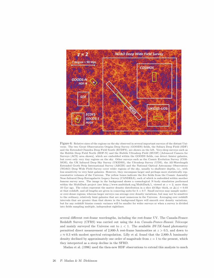
Figure 6: Relative sizes of the regions on the sky observed in several important surveys of the distant Uni-

verse. The two Great Observatories Origins Deep Survey (GOODS) fields, the Subaru Deep Field (SDF)

and the Extended Chandra Deep Field South (ECDFS), are shown on the left. Very-deep surveys such as

the Hubble Deep Field North (HDF-N) and the Hubble Ultradeep Field (HUDF) [Advanced Camera for

Surveys (ACS) area shown], which are embedded within the GOODS fields, can detect fainter galaxies,

but cover only very tiny regions on the sky. Other surveys such as the Cosmic Evolution Survey (COS-

MOS), the UK Infrared Deep Sky Survey (UKIDSS), the Ultradeep Survey (UDS), the All-Wavelength

Extended Groth Strip International Survey (AEGIS) and the National Optical Astronomy Observatory

(NOAO) Deep Wide Field Survey cover wider regions of the sky, usually to shallower depths, i.e., with

less sensitivity to very faint galaxies. However, they encompass larger and perhaps more statistically rep-

resentative volumes of the Universe. The yellow boxes indicate the five fields from the Cosmic Assembly

Near-Infrared Deep Extragalactic Legacy Survey (CANDELS), each of which is embedded within another

famous survey area. The image in the background shows a cosmological N-body simulation performed

within the MultiDark project (see http://www.multidark.org/MultiDark/), viewed at z = 2, more than

10 Gyr ago. The colors represent the matter density distribution in a slice 43-Mpc thick, or ∆(z) = 0.03

at that redshift, and all lengths are given in comoving units for h = 0.7. Small surveys may sample under-

or over-dense regions, whereas larger surveys can average over density variations, but may not be sensitive

to the ordinary, relatively faint galaxies that are most numerous in the Universe. Averaging over redshift

intervals that are greater than that shown in the background figure will smooth over density variations,

but for any redshift binsize cosmic variance will be smaller for wider surveys or when a survey is divided

into fields sampling multiple, independent sightlines.

several different rest-frame wavelengths, including the rest-frame UV. The Canada-France

Redshift Survey (CFRS) was carried out using the 4-m Canada-France-Hawaii Telescope

and mainly surveyed the Universe out to z < 1. The available BV IK-band photometry

permitted direct measurement of 2,800-A rest-frame luminosities at z > 0.5, and down to

z ≈ 0.3 with modest spectral extrapolation. Lilly et al. found that the 2,800-A luminosity

density declined by approximately one order of magnitude from z = 1 to the present, which

they interpreted as a steep decline in the SFRD.

Madau et al. (1996) used the then-new HDF observations to extend this analysis to much


http://www.multidark.org/MultiDark/

higher redshift. They employed color-selected LBG samples at 〈z〉 = 2.75 and 4. The deep

HST WFPC2 photometry allowed luminosities to be measured at 1,500A in the rest frame,

reaching fainter than contemporaneous ground-based LBG data at z ≈ 3 from Steidel et al.

(1996) and thus integrating further down the LF. Madau et al. (1996) quoted only lower

limits for the SFRD, without extrapolation to fainter luminosities (relatively small, given

the depth of the HDF imaging) and without correction for dust absorption (significant, but

at the time little known). Later analyses (e.g., Sawicki et al. 1997, Madau et al. 1998b,

Steidel et al. 1999) fit Schechter LFs to the photometric samples to extrapolate to total

UV luminosity densities. Connolly et al. (1997) and Pascarelle et al. (1998) combined the

optical HST imaging of the HDF with ground-based NIR data to improve photometric

redshift analyses in the “redshift desert” at 1 < z < 2, between the regime of Lilly et al.

(1996) and that of Madau et al. (1996).” Taken together, the HDF measurements at z > 1

and the CFRS measurements at z < 1 suggested a general “rise and fall” picture of a UV

luminosity density and, by inference, the cosmic SFH that peaked somewhere between z ≈ 1

and 2.

Various surveys subsequently extended this finding using other data sets or different

analyses. Several groups reanalyzed the HDF (and later the HDF-South) data in various

ways or made use of deeper spectroscopic surveys with the Keck telescope. Cowie et al.

(1999) and Wilson et al. (2002) combined Keck spectroscopy in several fields with deep

U -band imaging to measure shorter rest-frame UV wavelengths (,2000-2,500A) at z < 1

than were probed in the CFRS analysis of Lilly et al. (1996) and derived a shallower rate of

decline in the SFRD. Wolf et al. (2005) used 17-filter intermediate and broadband imaging

to obtain high-quality photometric redshifts at z < 1.25 in the Extended Chandra Deep

Field South and analyzed the 2,800-A luminosity density evolution.

Ideally, UV rest-frame observations at z < 1 should be done from space telescopes to

sample shorter UV wavelengths than those used in the ground-based studies by Lilly, Wil-

son, Wolf, and others. In early work, Treyer et al. (1998) and Sullivan et al. (2000) used

the FOCA balloon-born UV telescope to measure 2,000-A luminosity densities at z ≈ 0.15.

GALEX has since provided vastly more FUV data, including both wide-area and deeper

surveys. Wyder et al. (2005) combined GALEX all-sky imaging survey data with distances

from the 2dF Galaxy Redshift Survey (2dFGRS) over 56 deg2 to measure local (z ≈ 0.055)

LFs at 1,500A and 2,300 A. Budavari et al. (2005) analyzed a similar total sky area using

somewhat deeper GALEX data and SDSS-derived photometric redshifts to compute LFs

and densities at z < 0.25. Salim et al. (2007) and Robotham & Driver (2011) have since an-

alyzed much larger GALEX data with SDSS data to cover as much as 830 deg2. Robotham

& Driver presented a straightforward derivation of the UV luminosity function (UVLF)

and luminosity density, whereas Salim et al. used GALEX photometry as one ingredient to

derive SFRs and the total SFRD.

Arnouts et al. (2005) combined much deeper GALEX observations with spectroscopy from

the VIMOS VLT Deep Survey (VVDS) and derived 1,500-A rest-frame LFs at 0.2 < z < 1.2.

Schiminovich et al. (2005) integrated these LFs to determine the 1,500-A luminosity density,

measuring evolution consistent with ρFUV ∝ (1 + z)2.5. This remains the most direct and

frequently cited GALEX study of FUV luminosity densities at z < 1, which is somewhat

surprising, as there are many more deep GALEX observations in fields with extensive

spectroscopy (COSMOS, AEGIS, GOODS, etc.). Yet, to to our knowledge, there have

been no other published LFs. The Arnouts/Schiminovich analysis is admirable, but it used

only ∼ 1, 000 galaxies with spectroscopic redshifts over the whole range ∆z = 1 in a single

field covering 0.5 deg2. Hence, it may be subject to cosmic variance issues. This area is


quite ripe for further exploitation of existing archival data.

HST is the only other modern space telescope with UV capabilities, particularly with the

UVIS channel of the WFC3 camera. Until recently, only one 50-arcmin2 field in GOODS-

South has been surveyed to interesting depths to study distant galaxies (Hathi et al. 2010,

Oesch et al. 2010). At z < 1.4, where these data measure FUV rest-frame emission, the

survey volume and counting statistics are poor. These data have also been used for Lyman

break color selection at z ≈ 1.5–2. The analyses generally support relatively steep UVLFs

with α < −1.5 with large uncertainties. Expanded WFC3 UVIS observations in the HUDF

and GOODS-North field have been recently completed and should improve the existinf

measurements somewhat. A recent WFC3-UVIS survey of gravitationally lensed galaxies

behind the massive cluster Abell 1689 (Alavi et al. 2014) has been used for Lyman break

color selection to unprecedentedly faint FUV luminosities at z ≈ 2 to MAB ≈ −13, or

∼ 1, 000 times fainter than L∗ at that redshift. Alavi et al. (2014) found no turnover to the

LF down to those limits and measured a faint-end slope α = −1.56± 0.13.

Cucciati et al. (2012) analyzed a larger, deeper and more complete spectroscopic sample in

the same VVDS survey field studied by Arnouts et al. and Schiminovich et al. . They fit SED

models to multiband photometry from the U - to the K-bands to extrapolate flux density

measurements to FUV rest-frame wavelengths at z < 1.4. They demonstrated consistency

with the GALEX luminosity densities from Schiminovich but did not make direct use of

the GALEX data. Although the largest and deepest spectroscopic sample used to derive

UVLFs at 0 < z < 2, it is based on only one sightline and requires SED extrapolation to

rest frame 1,500A at lower redshifts. Tresse et al. (2007) presented a similar, earlier analysis

using shallower spectroscopy in two VVDS fields.

Over many years, Steidel and collaborators have carried out an extensive campaign of

Keck spectroscopy for Lyman break-selected galaxies, especially at z ≈ 2 and 3 (Steidel

et al. 2003, 2004). Their survey covers many widely-spread sightlines and provides excellent

control over cosmic variance. Among several LF analyses from these data, the most recent

and definitive are those of Reddy et al. (2008) and Reddy & Steidel (2009). These still rely

on deep photometric color-selected samples to probe the faint-end of the LF, but with a

degree of spectroscopic confirmation and calibration for brighter galaxies that is unmatched

by any other survey. The use of UV rest-frame selection means that any LBG-based study

will miss heavily dust-obscured star formation at these redshifts, but as a measure of the

evolving UV luminosity density the LBG surveys have provided the most robust method to

date.

At higher redshifts, 4 < z < 7, deep HST observations (discussed below) have dominated

surveys for LBGs in recent years, but several ground-based imaging programs have made

significant contributions, particularly surveying wider areas at (relatively) shallower depths

to constrain the bright end of the LF. The Subaru telescope and its SuPrime Cam imager

have been particularly important in this respect, although deep IR imaging from UKIRT

and the VLT have also been used. Notable examples (not an exhaustive list) include Ouchi

et al. (2004), Yoshida et al. (2006), Iwata et al. (2007) and McLure et al. (2009) at z = 4 to

6 and Ouchi et al. (2009), Castellano et al. (2010a,b), Bowler et al. (2012), and Tilvi et al.

(2013) at z ≈ 7.

The installation of the Advanced Camera for Surveys (ACS) enabled substantially more

efficient optical HST imaging that covers fields much wider than the original HDF. ACS

also offered significant gains in sensitivity at the reddest wavelengths, making Lyman break

selection practical out to z ≈ 6. Two major ACS surveys led to new derivations of the

cosmic SFRD. GOODS (Giavalisco et al. 2004b) observed two independent fields with com-


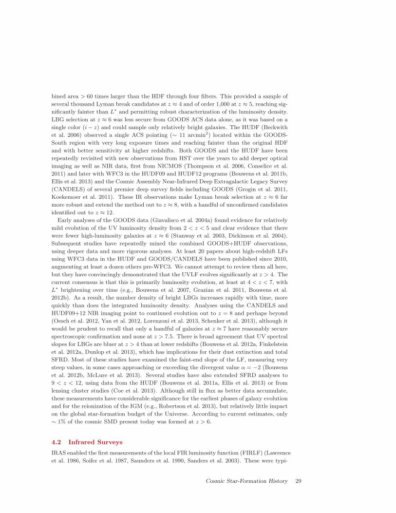
bined area > 60 times larger than the HDF through four filters. This provided a sample of

several thousand Lyman break candidates at z ≈ 4 and of order 1,000 at z ≈ 5, reaching sig-

nificantly fainter than L∗ and permitting robust characterization of the luminosity density.

LBG selection at z ≈ 6 was less secure from GOODS ACS data alone, as it was based on a

single color (i− z) and could sample only relatively bright galaxies. The HUDF (Beckwith

et al. 2006) observed a single ACS pointing (∼ 11 arcmin2) located within the GOODS-

South region with very long exposure times and reaching fainter than the original HDF

and with better sensitivity at higher redshifts. Both GOODS and the HUDF have been

repeatedly revisited with new observations from HST over the years to add deeper optical

imaging as well as NIR data, first from NICMOS (Thompson et al. 2006, Conselice et al.

2011) and later with WFC3 in the HUDF09 and HUDF12 programs (Bouwens et al. 2011b,

Ellis et al. 2013) and the Cosmic Assembly Near-Infrared Deep Extragalactic Legacy Survey

(CANDELS) of several premier deep survey fields including GOODS (Grogin et al. 2011,

Koekemoer et al. 2011). These IR observations make Lyman break selection at z ≈ 6 far

more robust and extend the method out to z ≈ 8, with a handful of unconfirmed candidates

identified out to z ≈ 12.

Early analyses of the GOODS data (Giavalisco et al. 2004a) found evidence for relatively

mild evolution of the UV luminosity density from 2 < z < 5 and clear evidence that there

were fewer high-luminosity galaxies at z ≈ 6 (Stanway et al. 2003, Dickinson et al. 2004).

Subsequent studies have repeatedly mined the combined GOODS+HUDF observations,

using deeper data and more rigorous analyses. At least 20 papers about high-redshift LFs

using WFC3 data in the HUDF and GOODS/CANDELS have been published since 2010,

augmenting at least a dozen others pre-WFC3. We cannot attempt to review them all here,

but they have convincingly demonstrated that the UVLF evolves significantly at z > 4. The

current consensus is that this is primarily luminosity evolution, at least at 4 < z < 7, with

L∗ brightening over time (e.g., Bouwens et al. 2007, Grazian et al. 2011, Bouwens et al.

2012b). As a result, the number density of bright LBGs increases rapidly with time, more

quickly than does the integrated luminosity density. Analyses using the CANDELS and

HUDF09+12 NIR imaging point to continued evolution out to z = 8 and perhaps beyond

(Oesch et al. 2012, Yan et al. 2012, Lorenzoni et al. 2013, Schenker et al. 2013), although it

would be prudent to recall that only a handful of galaxies at z ≈ 7 have reasonably secure

spectroscopic confirmation and none at z > 7.5. There is broad agreement that UV spectral

slopes for LBGs are bluer at z > 4 than at lower redshifts (Bouwens et al. 2012a, Finkelstein

et al. 2012a, Dunlop et al. 2013), which has implications for their dust extinction and total

SFRD. Most of these studies have examined the faint-end slope of the LF, measuring very

steep values, in some cases approaching or exceeding the divergent value α = −2 (Bouwens

et al. 2012b, McLure et al. 2013). Several studies have also extended SFRD analyses to

9 < z < 12, using data from the HUDF (Bouwens et al. 2011a, Ellis et al. 2013) or from

lensing cluster studies (Coe et al. 2013). Although still in flux as better data accumulate,

these measurements have considerable significance for the earliest phases of galaxy evolution

and for the reionization of the IGM (e.g., Robertson et al. 2013), but relatively little impact

on the global star-formation budget of the Universe. According to current estimates, only

∼ 1% of the cosmic SMD present today was formed at z > 6.

4.2 Infrared Surveys

IRAS enabled the first measurements of the local FIR luminosity function (FIRLF) (Lawrence

et al. 1986, Soifer et al. 1987, Saunders et al. 1990, Sanders et al. 2003). These were typi-


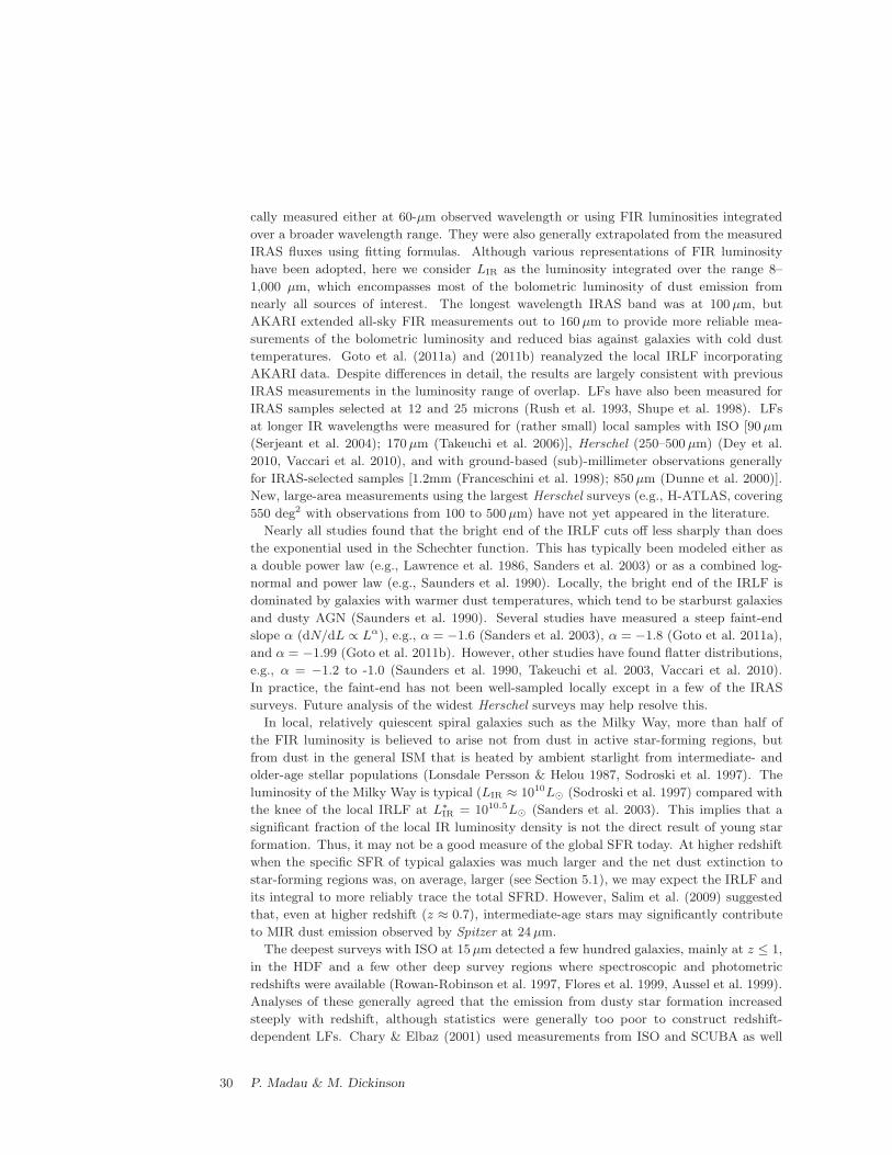
cally measured either at 60-µm observed wavelength or using FIR luminosities integrated

over a broader wavelength range. They were also generally extrapolated from the measured

IRAS fluxes using fitting formulas. Although various representations of FIR luminosity

have been adopted, here we consider LIR as the luminosity integrated over the range 8–

1,000 µm, which encompasses most of the bolometric luminosity of dust emission from

nearly all sources of interest. The longest wavelength IRAS band was at 100µm, but

AKARI extended all-sky FIR measurements out to 160µm to provide more reliable mea-

surements of the bolometric luminosity and reduced bias against galaxies with cold dust

temperatures. Goto et al. (2011a) and (2011b) reanalyzed the local IRLF incorporating

AKARI data. Despite differences in detail, the results are largely consistent with previous

IRAS measurements in the luminosity range of overlap. LFs have also been measured for

IRAS samples selected at 12 and 25 microns (Rush et al. 1993, Shupe et al. 1998). LFs

at longer IR wavelengths were measured for (rather small) local samples with ISO [90µm

(Serjeant et al. 2004); 170µm (Takeuchi et al. 2006)], Herschel (250–500 µm) (Dey et al.

2010, Vaccari et al. 2010), and with ground-based (sub)-millimeter observations generally

for IRAS-selected samples [1.2mm (Franceschini et al. 1998); 850µm (Dunne et al. 2000)].

New, large-area measurements using the largest Herschel surveys (e.g., H-ATLAS, covering

550 deg2 with observations from 100 to 500µm) have not yet appeared in the literature.

Nearly all studies found that the bright end of the IRLF cuts off less sharply than does

the exponential used in the Schechter function. This has typically been modeled either as

a double power law (e.g., Lawrence et al. 1986, Sanders et al. 2003) or as a combined log-

normal and power law (e.g., Saunders et al. 1990). Locally, the bright end of the IRLF is

dominated by galaxies with warmer dust temperatures, which tend to be starburst galaxies

and dusty AGN (Saunders et al. 1990). Several studies have measured a steep faint-end

slope α (dN/dL ∝ Lα), e.g., α = −1.6 (Sanders et al. 2003), α = −1.8 (Goto et al. 2011a),

and α = −1.99 (Goto et al. 2011b). However, other studies have found flatter distributions,

e.g., α = −1.2 to -1.0 (Saunders et al. 1990, Takeuchi et al. 2003, Vaccari et al. 2010).

In practice, the faint-end has not been well-sampled locally except in a few of the IRAS

surveys. Future analysis of the widest Herschel surveys may help resolve this.

In local, relatively quiescent spiral galaxies such as the Milky Way, more than half of

the FIR luminosity is believed to arise not from dust in active star-forming regions, but

from dust in the general ISM that is heated by ambient starlight from intermediate- and

older-age stellar populations (Lonsdale Persson & Helou 1987, Sodroski et al. 1997). The

luminosity of the Milky Way is typical (LIR ≈ 1010L⊙ (Sodroski et al. 1997) compared with

the knee of the local IRLF at L∗IR = 1010.5L⊙ (Sanders et al. 2003). This implies that a

significant fraction of the local IR luminosity density is not the direct result of young star

formation. Thus, it may not be a good measure of the global SFR today. At higher redshift

when the specific SFR of typical galaxies was much larger and the net dust extinction to

star-forming regions was, on average, larger (see Section 5.1), we may expect the IRLF and

its integral to more reliably trace the total SFRD. However, Salim et al. (2009) suggested

that, even at higher redshift (z ≈ 0.7), intermediate-age stars may significantly contribute

to MIR dust emission observed by Spitzer at 24µm.

The deepest surveys with ISO at 15µm detected a few hundred galaxies, mainly at z ≤ 1,

in the HDF and a few other deep survey regions where spectroscopic and photometric

redshifts were available (Rowan-Robinson et al. 1997, Flores et al. 1999, Aussel et al. 1999).

Analyses of these generally agreed that the emission from dusty star formation increased

steeply with redshift, although statistics were generally too poor to construct redshift-

dependent LFs. Chary & Elbaz (2001) used measurements from ISO and SCUBA as well


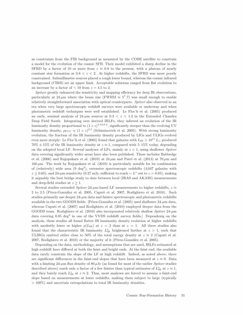
as constraints from the FIR background as measured by the COBE satellite to constrain

a model for the evolution of the cosmic SFH. Their model exhibited a sharp decline in the

SFRD by a factor of 10 or more from z ≈ 0.8 to the present, with a plateau of nearly

constant star formation at 0.8 < z < 2. At higher redshifts, the SFRD was more poorly

constrained. Submillimeter sources placed a rough lower bound, whereas the cosmic infrared

background (CIRB) set an upper limit. Acceptable solutions ranged from flat evolution to

an increase by a factor of ∼ 10 from z = 4.5 to 2.

Spitzer greatly enhanced the sensitivity and mapping efficiency for deep IR observations,

particularly at 24µm where the beam size (FWHM ≈ 5′′.7) was small enough to enable

relatively straightforward association with optical counterparts. Spitzer also observed in an

era when very large spectroscopic redshift surveys were available or underway and when

photometric redshift techniques were well established. Le Floc’h et al. (2005) produced

an early, seminal analysis of 24-µm sources at 0.3 < z < 1.2 in the Extended Chandra

Deep Field South. Integrating over derived IRLFs, they inferred an evolution of the IR

luminosity density proportional to (1+ z)3.9±0.4, significantly steeper than the evolving UV

luminosity density, ρFUV ∝ (1 + z)2.5 (Schiminovich et al. 2005). With strong luminosity

evolution, the fraction of the IR luminosity density produced by LIGs and ULIGs evolved

even more steeply: Le Floc’h et al. (2005) found that galaxies with LIR > 1011 L⊙ produced

70% ± 15% of the IR luminosity density at z ≈ 1, compared with 5–15% today, depending

on the adopted local LF. Several analyses of LFs, mainly at z < 1, using shallower Spitzer

data covering significantly wider areas have also been published. These includes Babbedge

et al. (2006) and Rujopakarn et al. (2010) at 24µm and Patel et al. (2013) at 70µm and

160µm. The work by Rujopakarn et al. (2010) is particularly notable for its combination

of (relatively) wide area (9 deg2), extensive spectroscopic redshifts (4,047 galaxies with

z ≤ 0.65), and 24-µm sensitivity (0.27 mJy, sufficient to reach ∼ L∗ out to z = 0.65), making

it arguably the best bridge study to date between local (IRAS and AKARI) measurements

and deep-field studies at z ≥ 1.

Several studies extended Spitzer 24-µm-based LF measurements to higher redshifts, z ≈

2 to 2.5 (Perez-Gonzalez et al. 2005, Caputi et al. 2007, Rodighiero et al. 2010). Such

studies primarily use deeper 24-µm data and fainter spectroscopic and photometric redshifts

available in the two GOODS fields. [Perez-Gonzalez et al. (2005) used shallower 24-µm data,

whereas Caputi et al. (2007) and Rodighiero et al. (2010) employed deeper data from the

GOODS team. Rodighiero et al. (2010) also incorporated relatively shallow Spitzer 24-µm

data covering 0.85 deg2 in one of the VVDS redshift survey fields.] Dependenig on the

analysis, these studies all found flatter IR luminosity density evolution at higher redshifts

with modestly lower or higher ρ(LIR) at z = 2 than at z = 1. All three studies also

found that the characteristic IR luminosity L∗IR brightened further at z > 1, such that

ULIRGs emitted either close to 50% of the total energy density at z ≈ 2 (Caputi et al.

2007, Rodighiero et al. 2010) or the majority of it (Perez-Gonzalez et al. 2005).

Depending on the data, methodology, and assumptions that are used, IRLFs estimated at

high redshift have differed at both the faint and bright ends. At the faint end, the available

data rarely constrain the slope of the LF at high redshift. Indeed, as noted above, there

are significant differences in the faint-end slopes that have been measured at z ≈ 0. Data

with a limiting 24-µm flux density of 80µJy (as found for most of the earlier Spitzer studies

described above) reach only a factor of a few fainter than typical estimates of L∗IR at z ≈ 1,

and they barely reach L∗IR at z ≈ 2. Thus, most analyses are forced to assume a faint-end

slope based on measurements at lower redshifts, making them subject to large (typically

> 100%) and uncertain extrapolations to total IR luminosity densities.


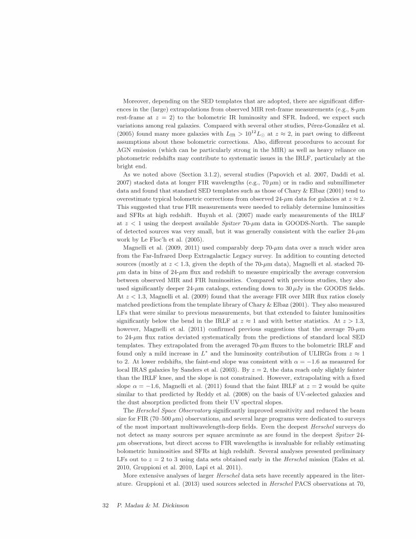
Moreover, depending on the SED templates that are adopted, there are significant differ-

ences in the (large) extrapolations from observed MIR rest-frame measurements (e.g., 8-µm

rest-frame at z = 2) to the bolometric IR luminosity and SFR. Indeed, we expect such

variations among real galaxies. Compared with several other studies, Perez-Gonzalez et al.

(2005) found many more galaxies with LIR > 1012L⊙ at z ≈ 2, in part owing to different

assumptions about these bolometric corrections. Also, different procedures to account for

AGN emission (which can be particularly strong in the MIR) as well as heavy reliance on

photometric redshifts may contribute to systematic issues in the IRLF, particularly at the

bright end.

As we noted above (Section 3.1.2), several studies (Papovich et al. 2007, Daddi et al.

2007) stacked data at longer FIR wavelengths (e.g., 70µm) or in radio and submillimeter

data and found that standard SED templates such as those of Chary & Elbaz (2001) tend to

overestimate typical bolometric corrections from observed 24-µm data for galaxies at z ≈ 2.

This suggested that true FIR measurements were needed to reliably determine luminosities

and SFRs at high redshift. Huynh et al. (2007) made early measurements of the IRLF

at z < 1 using the deepest available Spitzer 70-µm data in GOODS-North. The sample

of detected sources was very small, but it was generally consistent with the earlier 24-µm

work by Le Floc’h et al. (2005).

Magnelli et al. (2009, 2011) used comparably deep 70-µm data over a much wider area

from the Far-Infrared Deep Extragalactic Legacy survey. In addition to counting detected

sources (mostly at z < 1.3, given the depth of the 70-µm data), Magnelli et al. stacked 70-

µm data in bins of 24-µm flux and redshift to measure empirically the average conversion

between observed MIR and FIR luminosities. Compared with previous studies, they also

used significantly deeper 24-µm catalogs, extending down to 30µJy in the GOODS fields.

At z < 1.3, Magnelli et al. (2009) found that the average FIR over MIR flux ratios closely

matched predictions from the template library of Chary & Elbaz (2001). They also measured

LFs that were similar to previous measurements, but that extended to fainter luminosities

significantly below the bend in the IRLF at z ≈ 1 and with better statistics. At z > 1.3,

however, Magnelli et al. (2011) confirmed previous suggestions that the average 70-µm

to 24-µm flux ratios deviated systematically from the predictions of standard local SED

templates. They extrapolated from the averaged 70-µm fluxes to the bolometric IRLF and

found only a mild increase in L∗ and the luminosity contribution of ULIRGs from z ≈ 1

to 2. At lower redshifts, the faint-end slope was consistent with α = −1.6 as measured for

local IRAS galaxies by Sanders et al. (2003). By z = 2, the data reach only slightly fainter

than the IRLF knee, and the slope is not constrained. However, extrapolating with a fixed

slope α = −1.6, Magnelli et al. (2011) found that the faint IRLF at z = 2 would be quite

similar to that predicted by Reddy et al. (2008) on the basis of UV-selected galaxies and

the dust absorption predicted from their UV spectral slopes.

The Herschel Space Observatory significantly improved sensitivity and reduced the beam

size for FIR (70–500 µm) observations, and several large programs were dedicated to surveys

of the most important multiwavelength-deep fields. Even the deepest Herschel surveys do

not detect as many sources per square arcminute as are found in the deepest Spitzer 24-

µm observations, but direct access to FIR wavelengths is invaluable for reliably estimating

bolometric luminosities and SFRs at high redshift. Several analyses presented preliminary

LFs out to z = 2 to 3 using data sets obtained early in the Herschel mission (Eales et al.

2010, Gruppioni et al. 2010, Lapi et al. 2011).

More extensive analyses of larger Herschel data sets have recently appeared in the liter-

ature. Gruppioni et al. (2013) used sources selected in Herschel PACS observations at 70,


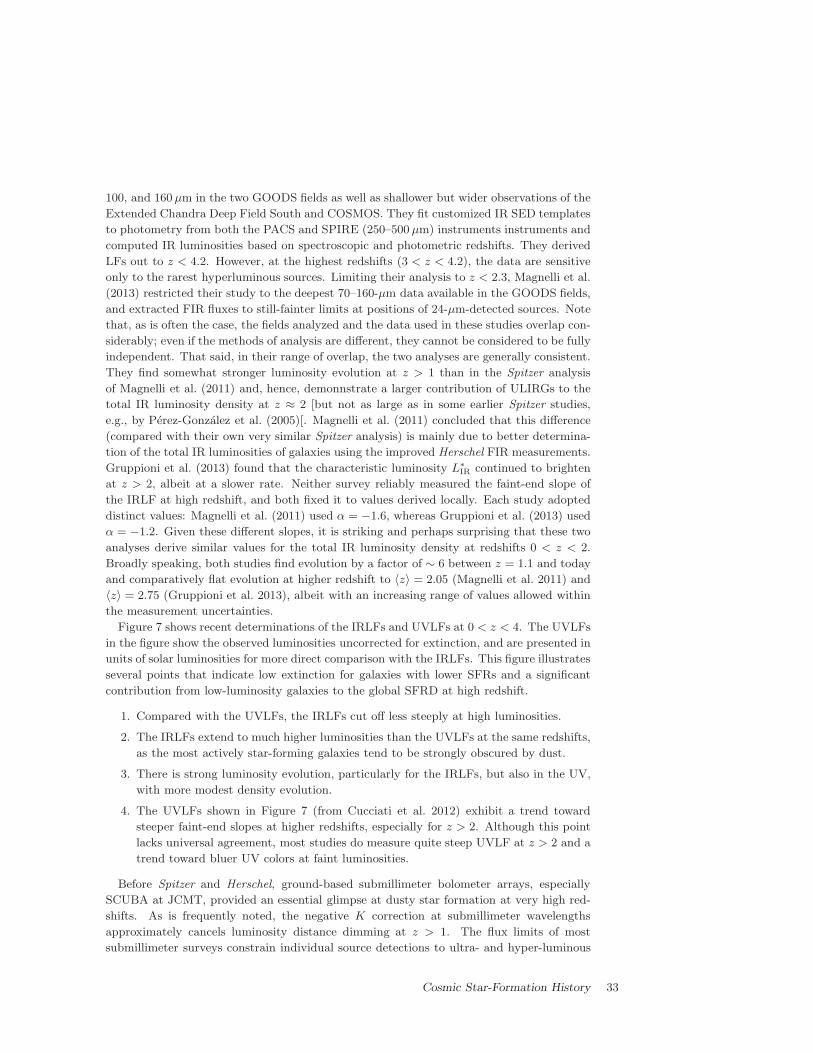
100, and 160µm in the two GOODS fields as well as shallower but wider observations of the

Extended Chandra Deep Field South and COSMOS. They fit customized IR SED templates

to photometry from both the PACS and SPIRE (250–500 µm) instruments instruments and

computed IR luminosities based on spectroscopic and photometric redshifts. They derived

LFs out to z < 4.2. However, at the highest redshifts (3 < z < 4.2), the data are sensitive

only to the rarest hyperluminous sources. Limiting their analysis to z < 2.3, Magnelli et al.

(2013) restricted their study to the deepest 70–160-µm data available in the GOODS fields,

and extracted FIR fluxes to still-fainter limits at positions of 24-µm-detected sources. Note

that, as is often the case, the fields analyzed and the data used in these studies overlap con-

siderably; even if the methods of analysis are different, they cannot be considered to be fully

independent. That said, in their range of overlap, the two analyses are generally consistent.

They find somewhat stronger luminosity evolution at z > 1 than in the Spitzer analysis

of Magnelli et al. (2011) and, hence, demonnstrate a larger contribution of ULIRGs to the

total IR luminosity density at z ≈ 2 [but not as large as in some earlier Spitzer studies,

e.g., by Perez-Gonzalez et al. (2005)[. Magnelli et al. (2011) concluded that this difference

(compared with their own very similar Spitzer analysis) is mainly due to better determina-

tion of the total IR luminosities of galaxies using the improved Herschel FIR measurements.

Gruppioni et al. (2013) found that the characteristic luminosity L∗IR continued to brighten

at z > 2, albeit at a slower rate. Neither survey reliably measured the faint-end slope of

the IRLF at high redshift, and both fixed it to values derived locally. Each study adopted

distinct values: Magnelli et al. (2011) used α = −1.6, whereas Gruppioni et al. (2013) used

α = −1.2. Given these different slopes, it is striking and perhaps surprising that these two

analyses derive similar values for the total IR luminosity density at redshifts 0 < z < 2.

Broadly speaking, both studies find evolution by a factor of ∼ 6 between z = 1.1 and today

and comparatively flat evolution at higher redshift to 〈z〉 = 2.05 (Magnelli et al. 2011) and

〈z〉 = 2.75 (Gruppioni et al. 2013), albeit with an increasing range of values allowed within

the measurement uncertainties.

Figure 7 shows recent determinations of the IRLFs and UVLFs at 0 < z < 4. The UVLFs

in the figure show the observed luminosities uncorrected for extinction, and are presented in

units of solar luminosities for more direct comparison with the IRLFs. This figure illustrates

several points that indicate low extinction for galaxies with lower SFRs and a significant

contribution from low-luminosity galaxies to the global SFRD at high redshift.

1. Compared with the UVLFs, the IRLFs cut off less steeply at high luminosities.

2. The IRLFs extend to much higher luminosities than the UVLFs at the same redshifts,

as the most actively star-forming galaxies tend to be strongly obscured by dust.

3. There is strong luminosity evolution, particularly for the IRLFs, but also in the UV,

with more modest density evolution.

4. The UVLFs shown in Figure 7 (from Cucciati et al. 2012) exhibit a trend toward

steeper faint-end slopes at higher redshifts, especially for z > 2. Although this point

lacks universal agreement, most studies do measure quite steep UVLF at z > 2 and a

trend toward bluer UV colors at faint luminosities.

Before Spitzer and Herschel, ground-based submillimeter bolometer arrays, especially

SCUBA at JCMT, provided an essential glimpse at dusty star formation at very high red-

shifts. As is frequently noted, the negative K correction at submillimeter wavelengths

approximately cancels luminosity distance dimming at z > 1. The flux limits of most

submillimeter surveys constrain individual source detections to ultra- and hyper-luminous


galaxies, so that only the tip of the IRLF is sampled. In practice, the greatest limitation

for deriving LFs or SFRD is identifying galaxy counterparts to submillimeter sources and

measuring their redshifts. This limitation is due mainly to the large beam-size of single-dish

submillimeter observations, but it is also due to the fact that the optical counterparts are

often very faint and sometimes invisible. Another consequence of the negative K correction

is that substantial redshift uncertainties translate to only relatively small uncertainties in

the bolometric luminosity. Hence, using radio-identified counterparts and very rough radio-

millimetric redshift estimates, Barger et al. (2000) were able to make plausible estimates

of the SFRD from submillimeter sources in broad redshift bins. Barger et al. (2012) re-

cently updated their findings using a complete submillimeter galaxy (SMG) sample with

accurate interferometric positions from the Submillimeter Array and with more extensive

redshift information, made possible in part thanks to recent advances in millimetric CO

spectroscopy. Chapman et al. (2005) measured optical spectroscopic redshifts for a sample

of radio-identified SMGs, and derived the first LF at 〈z〉 = 0.9 and 〈z〉 = 2.5. These esti-

mates were recently updated by Wardlow et al. (2011) using (mainly) photometric redshifts

for another well-defined SMG sample. These analyses demonstrated a significant contribu-

tion of dusty SMGs to the cosmic SFRD at high redshift, mainly limited to z . 4. However,

recent discoveries of substantial numbers of SMGs out to z = 6.3 (e.g., Riechers et al. 2013)

suggest that the dusty ultraluminous population may be important even in the first few

billion years of the cosmic SFH.

Although direct FIR detection of individual sources at z ≫ 2 is limited to the most

extremely luminous objects (Figure 1), the CIRB provides additional constraints on dusty

star formation at the highest redshifts (Pei et al. 1999, Gispert et al. 2000). FIR source

counts and the CIRB were reviewed by Lagache et al. (2005) and recent results from Herschel

are reviewed by Lutz (2014) in this volume, so we only briefly discuss this topic here.

Sources directly detected by Herschel in the deepest observations resolve ∼ 75% of the

CIRB at 100 and 160µm (Berta et al. 2011, Magnelli et al. 2013), albeit with significant

uncertainties at 100µm. Stacking Herschel data at the position of sources detected by

Spitzer at 24µm detects an even larger fraction that, with modest extrapolation, can account

for the entire CIRB at these wavelengths. At 250 to 500µm, where confusion is more severe

in Herschel SPIRE data, the directly resolved fractions are smaller (from 15% to 5% at 250

to 500µm), whereas stacking detects 73% to 55%. Again, an extrapolation is consistent

with resolving the entire background (Bethermin et al. 2012). Because the deepest Herschel

observations were carried out in fields such as GOODS and COSMOS with exceptional

ancillary data, it is possible to stack in bins of photometric redshift, to constrain the redshift

distribution of the CIRB emission. At higher redshifts, the peak of dust emission from

galaxies shifts to longer FIR and submillimeter wavelengths, and the fractional contribution

of more distant galaxies increases with the wavelength of the bandpass analyzed. Combining

data from Spitzer through Herschel to ground-based submillimeter observations, Bethermin

et al. (2012) estimated that 4.7 ± 2.0 nW m−2 sr−1, or 17+11−9 % of the integrated CIRB,

is produced by galaxies at z > 2. Although the fraction is small, it still allows for a

significant amount of dusty star formation to take place at z > 2, beyond what is seen

in directly detected sources. However, the 24-µm sources used for these stacking analyses

are also subject to strong k–correction dimming at z > 2. Thus, a larger fraction of the

high-redshift CIRB may have been missed.


4.3 Emission Line Surveys

Among the nebular emission lines that have been most frequently used to quantify SFRs at

high redshift, Hα is arguably the most useful (see Section 3.1.4). Lines from other elements,

most commonly [OII] 3,727 A, have also been used to measure the cosmic SFR (e.g., Hogg

et al. 1998), but their more complex dependence on metallicity and ISM conditions as well

as their larger extinction make them problematic. Narrow-band Lyα surveys are popular

at high redshift, but Lyα is so strongly subject to resonant scattering and extinction that

it must always be regarded as setting only a lower limit on the true SFR.

Hα is accessible with optical observations only at z < 0.5, and NIR observations are

needed to follow it out to higher redshifts (z . 2.5). Recent technological developments in

IR instrumentation have significantly increased the potential for such measurements. A new

generation of wide-field imagers using mosaics of IR arrays is now operating on 4-m- and

8-m-class telescopes (e.g., UKIRTWFCAM, CFHT WIRCAM, NOAO NEWFIRM, VISTA

VIRCAM, VLT HAWK-I), thereby significantly increasing the comoving volumes accessible

for deep narrow-band imaging. NIR multiobject spectrographs are now becoming mature

and efficient (e.g., Subaru MOIRCS and FMOS, Keck MOSFIRE, VLT KMOS, LBT LUCI).

Slitless grism spectroscopy with WFC3 on the HST can measure faint Hα lines out to z < 1.5

for all objects within its field of view. Each method has advantages and disadvantages.

Narrow-band imaging surveys are tuned to specific, narrow redshift ranges and are strongly

subject to density variations due to line-of-sight clustering effects. Flux calibration for

objects whose redshifts place emission lines in the wings of the narrow bandpasses can

also be problematic. Only statistical corrections can be made for the flux contribution from

[NII] or for stellar absorption. Multislit spectroscopy is subject to slit losses that complicate

measurements of integrated line fluxes, and atmospheric absorption and emission significant

limit the accessible redshifts and can introduce complicated selection effects. (The new

VLT KMOS spectrograph uses multiple deployable integral field units, thus eliminating

slit-loss concerns, and may prove to be a valuable tool for Hα surveys.) HST WFC3 slitless

spectroscopy avoids concerns about the atmosphere and slit losses, but deep observations

covering adequately large solid angles are time-intensive. As of this writing, results on Hα

LFs from the largest ongoing programs [WISPS (Atek et al. 2010) and 3D-HST (Brammer

et al. 2012)] have not appeared in the literature to supersede earlier HST NICMOS results

(Yan et al. 1999, Hopkins et al. 2000, Shim et al. 2009). With all methods, reliable extinction

corrections depend on the measurement of the Balmer decrement (the ratio of Hα to Hβ

line fluxes). This is rarely available for narrow-band surveys, but it is sometimes available

for spectroscopic samples. However, in such cases, the sample selection is often limited by

the weaker Hβ line. Hence, statistical corrections are often adopted. AGN and LINERs

can also contribute significantly to the samples of emission line galaxies and can be reliably

taken into account only using high-quality spectroscopic data to measure line-excitation

diagnostics. Most careful studies of the local galaxy population using spectroscopy from

SDSS or GAMA (see below) have done this, but it is rarely possible at higher redshifts.

Thus, most studies have resorted to statistical corrections or none at all.

Much literature discusses LF and SFRD measurements from Hα, [OII] and [OIII], and we

note only selected works here. Gunawardhana et al. (2013) included a thorough and up-to-

date compilation of these measurements at low and high redshifts. Using objective prism

photographic data, Gallego et al. (1995) presented an important early study of the local Hα

LF. Subsequently, the SDSS provided a vast number of spectroscopic redshifts and line-flux

measurements, although the small aperture size of the spectroscopic fibers requires careful


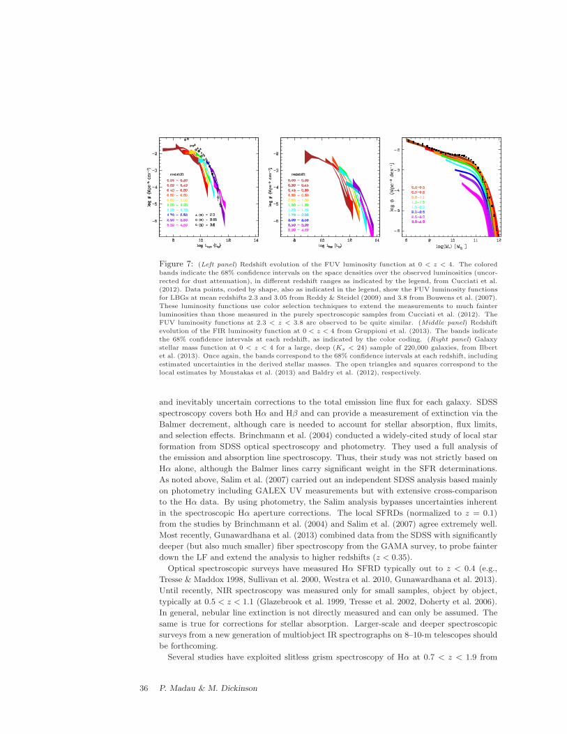
Figure 7: (Left panel) Redshift evolution of the FUV luminosity function at 0 < z < 4. The colored

bands indicate the 68% confidence intervals on the space densities over the observed luminosities (uncor-

rected for dust attenuation), in different redshift ranges as indicated by the legend, from Cucciati et al.

(2012). Data points, coded by shape, also as indicated in the legend, show the FUV luminosity functions

for LBGs at mean redshifts 2.3 and 3.05 from Reddy & Steidel (2009) and 3.8 from Bouwens et al. (2007).

These luminosity functions use color selection techniques to extend the measurements to much fainter

luminosities than those measured in the purely spectroscopic samples from Cucciati et al. (2012). The

FUV luminosity functions at 2.3 < z < 3.8 are observed to be quite similar. (Middle panel) Redshift

evolution of the FIR luminosity function at 0 < z < 4 from Gruppioni et al. (2013). The bands indicate

the 68% confidence intervals at each redshift, as indicated by the color coding. (Right panel) Galaxy

stellar mass function at 0 < z < 4 for a large, deep (Ks < 24) sample of 220,000 galaxies, from Ilbert

et al. (2013). Once again, the bands correspond to the 68% confidence intervals at each redshift, including

estimated uncertainties in the derived stellar masses. The open triangles and squares correspond to the

local estimates by Moustakas et al. (2013) and Baldry et al. (2012), respectively.

and inevitably uncertain corrections to the total emission line flux for each galaxy. SDSS

spectroscopy covers both Hα and Hβ and can provide a measurement of extinction via the

Balmer decrement, although care is needed to account for stellar absorption, flux limits,

and selection effects. Brinchmann et al. (2004) conducted a widely-cited study of local star

formation from SDSS optical spectroscopy and photometry. They used a full analysis of

the emission and absorption line spectroscopy. Thus, their study was not strictly based on

Hα alone, although the Balmer lines carry significant weight in the SFR determinations.

As noted above, Salim et al. (2007) carried out an independent SDSS analysis based mainly

on photometry including GALEX UV measurements but with extensive cross-comparison

to the Hα data. By using photometry, the Salim analysis bypasses uncertainties inherent

in the spectroscopic Hα aperture corrections. The local SFRDs (normalized to z = 0.1)

from the studies by Brinchmann et al. (2004) and Salim et al. (2007) agree extremely well.

Most recently, Gunawardhana et al. (2013) combined data from the SDSS with significantly

deeper (but also much smaller) fiber spectroscopy from the GAMA survey, to probe fainter

down the LF and extend the analysis to higher redshifts (z < 0.35).

Optical spectroscopic surveys have measured Hα SFRD typically out to z < 0.4 (e.g.,

Tresse & Maddox 1998, Sullivan et al. 2000, Westra et al. 2010, Gunawardhana et al. 2013).

Until recently, NIR spectroscopy was measured only for small samples, object by object,

typically at 0.5 < z < 1.1 (Glazebrook et al. 1999, Tresse et al. 2002, Doherty et al. 2006).

In general, nebular line extinction is not directly measured and can only be assumed. The

same is true for corrections for stellar absorption. Larger-scale and deeper spectroscopic

surveys from a new generation of multiobject IR spectrographs on 8–10-m telescopes should

be forthcoming.

Several studies have exploited slitless grism spectroscopy of Hα at 0.7 < z < 1.9 from


the HST NICMOS instrument (Yan et al. 1999, Hopkins et al. 2000, Shim et al. 2009).

These studies are of small but relatively unbiased samples that are observed with relatively

uniform sensitivity over a broad redshift range and without concerns for flux losses due to

a finite spectrograph slit size. Once again, direct measurements of extinction are generally

unavailable, and the low-resolution slitless spectroscopy inextricably blends Hα with [NII],

thus requiring purely statistical corrections. New, more sensitive grism surveys with HST

WFC3 that cover larger solid angles are under way.

The largest number of high-redshift measurements has come from narrow-band imaging

surveys, using wide-field CCD cameras out to z ≈ 0.4 and with IR arrays at higher red-

shifts. These are generally carried out using filters that fit into spectral windows relatively

unaffected by atmospheric absorption or emission and that correspond to specific redshifts

(z = 0.24, 0.40, 0.84, 1.47, and 2.23 are all common). Using a new generation of wide-field

imagers, the current state-of-the-art Hα surveys include those of Ly et al. (2007, 2011),

Hayes et al. (2010), and Sobral et al. (2013). The latter survey (HiZELS) combines data

from Subaru Suprime-Cam (z = 0.40) and UKIRT WFCAM (z = 0.84, 1.47 and 2.23). It

covers ∼ 2 deg2 in two survey fields, with deeper but narrower (0.03 deg2) observations at

z = 2.23 from the VLT and its HAWK-I imager. Between 500 and 1750 Hα emitters are de-

tected in each redshift window, thereby providing good statistics. These authors measured

a steady increase in the characteristic luminosity L∗(Hα) with redshift and a faint-end slope

α ≈ 1.6 that is constant with redshift, and is also similar to that found in most of the UV

continuum surveys.

4.4 Radio Surveys

Centimeter-wavelength radio continuum emission from star-forming galaxies arises from a

combination of flat-spectrum free-free emission, which is prominent at high frequencies,

and steep spectrum synchrotron emission, which dominates at lower frequencies. Although

the free-free emission should be a direct tracer of SFRs, it has been impractical to observe

this at high redshift. However, the improved high-frequency sensitivity of the Jansky VLA

should open this capability in the future. The lower-frequency emission arises mainly as a

consequence of SNe. As such, it is also related to the SFR. In practice, its calibration as

an SFR measurement is primarily empirical, e.g., based on the tight correlation observed

between radio and FIR emission for IRAS-selected galaxies in the local Universe (e.g., Yun

et al. 2001). This correlation together with insensitivity to dust extinction make radio

emission an attractive wavelength for studying star formation.

Problematically, AGN can also produce powerful radio emission. Locally, radio sources

with Lν(1.4 GHz) > 1023 W Hz−1 are predominantly AGN. This radio luminosity corre-

sponds to a SFR > 94 M⊙ year−1, using the conversion factor from Murphy et al. (2011)

scaled to a Salpeter IMF. Such galaxies are extremely rare locally, so very powerful radio

sources are commonly excluded as likely AGN. However, at z > 1, galaxies with these SFRs

(corresponding to ULIRGs in terms of their IR luminosities) are common, even “normal”

(see Section 3.1.2). Thus, it is problematic to disregard them simply on the basis of their

radio emission. Other considerations are needed to distinguish AGN from star-forming ra-

dio sources, such as radio spectral index, radio morphology, or radio/IR flux ratios, but

these are all more difficult to measure, especially for very faint sources.

The local radio LF has been used to estimate the current SFRD in many studies (for recent

examples, see Machalski & Godlowski 2000, Condon et al. 2002, Sadler et al. 2002, Serjeant

et al. 2002, Mauch & Sadler 2007). In these studies, the authors carefully employed various


criteria to separate AGN from star-forming galaxies. Data were often compared with IRAS

IR measurements and excluded objects with a radio excess relative to their IR luminosities.

At z > 1, even the deepest VLA surveys have been able to detect galaxies with SFRs only

& 100 M⊙ year−1 (Figure 1) and & 1000 M⊙ year−1 at z > 3, although the Jansky VLA is

now pushing to fainter sensitivities. Haarsma et al. (2000) were among the first to combine

very deep VLA observations with spectroscopic and photometric redshift information to

derive radio LFs and the cosmic SFRD at high redshift, primarily at 0.3 < z < 0.8.

However, they also considered one very broad bin from 1 < z < 4.4. Based on individually

detected radio sources, this work was updated in later studies that took advantage of more

extensive multiwavelength data to distinguish AGN from star-forming galaxies. Seymour

et al. (2008) identified AGN based on radio spectral indexes, radio morphology, and radio

to NIR and MIR flux ratios. Smolcic et al. (2009) used optical SED criteria to identify star-

forming galaxies detected in VLA 1.4 GHz data for COSMOS, at more modest redshifts,

z < 1.3. Seymour et al. (2008) assumed pure luminosity evolution for the LF, consistent

with the measurements by Smolcic et al. (2009) (and earlier by Haarsma et al. 2000). All

these studies found broad agreement between the radio SFRD evolution and optical and

IR surveys, noting a steep decline from z = 1 to 0; Seymour et al. (2008) measured a peak

SFRD at z ≈ 1.5, albeit with large uncertainties.

Other studies have used radio stacking to probe to fainter luminosities, below the detec-

tion limits for individual sources – particularly, stacking for NIR samples that approximate

stellar mass selection. Here, the assumption is that, as in the local Universe, radio sources

at fainter luminosities will primarily trace star formation, with relatively little AGN con-

tribution. Dunne et al. (2009) stacked VLA 1.4 GHz and GMRT 610 MHz data for K-

band-selected sources in bins of redshift and K-band luminosity. They found a linear (but

redshift-dependent) relation between radio and NIR luminosity. Using a measurement of

the evolving K-band LF from the same data set, they then used this radio/NIR ratio to

extrapolate the observations to the total radio luminosity density and SFRD. Karim et al.

(2011) used a large 1.4-GHz survey of COSMOS and a Spitzer 3.6-µm–selected sample to

carry out the most extensive study of this sort to date. Stacking in bins of stellar mass and

photometric redshift and converting the mean radio fluxes to SFRs, they extensively ana-

lyzed the SFR–M∗ correlation, and used this and the evolving stellar mass function (SMF)

(from Ilbert et al. 2010) to compute the integrated SFRD. Dunne et al. (2009) measured

a steady increase in the SFRD from z ≈ 0 to a peak at z ≈ 1.5 that declined at higher

redshift to z ≈ 4. By contrast, Karim et al. (2011) found a monotonic decline in the SFRD

from z = 3 to today.

4.5 Stellar Mass Density Surveys

As the technology of NIR detectors advanced, so did surveys that used NIR photometry to

better sample galaxies by stellar mass at both low and high redshifts (e.g., Cowie et al. 1996,

Gavazzi et al. 1996). However, it was not until the turn of the millennium that authors

started to routinely use stellar population synthesis models to convert photometry and red-

shift information to stellar masses for large samples of galaxies, especially at high redshift.

Before the era of large, modern redshift surveys such as the SDSS and the 2dFGRS, several

authors made estimates of the local baryonic and SMDs (Persic & Salucci 1992, Fukugita

et al. 1998, Salucci & Persic 1999). This effort accelerated, however, as new spectroscopic

surveys mapped the local Universe. Cole et al. (2001) used 2dFGRS redshifts and NIR

photometry from 2MASS to measure the local K-band LF more accurately than had pre-


viously been possible. Then, using stellar population modeling, they inferred stellar masses

from the galaxy colors and luminosities and derived the local galaxy stellar mass function

(GSMF) and the local comoving SMD. Bell et al. (2003) did the same using SDSS and

2MASS. Many studies have subsequently derived the GSMF from incrementally improv-

ing SDSS data releases, using additional ancillary data and a variety of methods for stellar

population modeling; mass-to-light ratios are sometimes derived from photometry and from

the SDSS spectra (Panter et al. 2007, Baldry et al. 2008, Li & White 2009). Moustakas

et al. (2013) incorporated photometry from the ultraviolet (GALEX) to the MIR (WISE)

in their analysis of the SDSS GSMF. Baldry et al. (2012) analyzed a sample from GAMA,

a wide-area spectroscopic survey extending significantly fainter than the SDSS, modeling

M/L from optical SDSS photometry. As the samples have grown larger, more elaborate

functional forms have been fit to the GSMF, including double and even triple Schechter

functions, and there is some evidence that the GSMF slope at low masses (< 109 M⊙)

may be steeper than was previously believed (e.g., α = −1.47) (Baldry et al. 2012). Other

authors have modeled stellar populations for ensembles of galaxies rather than deriving

individual galaxy stellar masses, e.g., by fitting the integrated local luminosity densities

for the entire local volume from UV to NIR wavelengths (Baldry & Glazebrook 2003) or

by modeling coadded SDSS spectra in bins of luminosity, velocity dispersion, and 4,000-A

break strength (Gallazzi et al. 2008).

At higher redshifts, Brinchmann & Ellis (2000) derived stellar masses for galaxies at z < 1

in fields with both HST and NIR imaging. As expected given the declining cosmic SFRD

at those redshifts, they found relatively little evolution in the integrated mass density at

0.4 < z < 0.9, but a marked evolution in the mass breakdown by morphological type.

Cohen (2002) similarly found no significant evolution in the SMD at 0.25 < z < 1.05.

Because the cosmic SFRD declines steeply with time at z < 1, relatively little new stellar

mass accumulates in the late stages of cosmic history. Moustakas et al. (2013) recently

broke new ground with a low-resolution prism spectroscopic survey measuring ∼ 40, 000

redshifts for galaxies at 0.2 < z < 1 in five fields with Spitzer IRAC photometry covering

5.5 deg2. Even with such outstanding data, the evolution in the overall SMF at 0 < z < 1

is nearly imperceptible, but the migration of galaxies from the star-forming to the quiescent

population is confirmed with exquisite detail.

Sawicki & Yee (1998), Giallongo et al. (1998), Papovich et al. (2001), and Shapley et al.

(2001) pioneered the use of stellar population models to derive stellar masses for LBGs at

z ≈ 2–3. Giallongo et al. (1998) computed comoving SMDs out to z ≈ 4 for galaxies

from a relatively bright, optically-selected sample, and measured steep evolution, but did

not attempt to correct for unobserved galaxies fainter than the limits of their data. Sub-

sequently, Dickinson et al. (2003), Fontana et al. (2003), and Rudnick et al. (2003) used

the deepest NIR imaging then available for the two HDFs, HST NICMOS (HDF-N) and

VLT ISAAC (HDF-S), together with extensive photometric and spectroscopic redshifts to

derive the comoving SMD in several redshift bins out to z ≈ 3. Strong evolution was found

over that longer redshift baseline; the SMD at z ≈ 3 measured in the range 5 to 15% of

its present-day value, although a somewhat broader range of values would be permitted if

systematic assumptions about the galaxy SFHs or stellar metallicities were pushed well be-

yond the range of models used for standard analysis. The SMD reached half its present-day

value somewhere between z = 2 and 1. Strong cosmic variance in these small fields was

also evident: At z > 2, red galaxies with high mass-to-light ratios were nearly absent in

the HDF-N but were found in moderate abundance in the HDF-S. By contrast, the corre-

sponding SMDs differed substantially. This indicated the importance of surveying larger


fields and more sightlines, but obtaining IR imaging to satisfactory depth over these larger

regions of sky has proven to be very challenging and has required another decade of effort.

The launch of Spitzer and the impressive performance of its IRAC camera for imaging

at 3.6 to 8µm made it possible to measure rest-frame NIR photometry for galaxies at

high redshift, and major public survey imaging campaigns such as GOODS, S-COSMOS,

and SWIRE produced widely-accessible and heavily-used imaging data sets spanning a

wide range of area–depth parameter space, ideal for deriving SMFs and densities at high

redshift. Indeed, NIR imaging has struggled to catch up with IRAC in terms of comparable

area–depth coverage. Despite the vast swaths of telescope time that have been invested

in obtaining NIR data on popular fields such as GOODS and COSMOS, imaging at 1 to

2.5µm still tends to fall short of Spitzer’s sensitivity at 3.6 and 4.5µm. At z > 4.5, the

ground-based K-band samples rest-frame ultraviolet wavelengths, and IRAC offers the only

viable way to measure optical rest-frame light to constrain stellar masses.

From 2006 onward, most (although not all) papers on SMFs and densities at high redshift

have made use of IRAC data – often in the same survey fields that are repeatedly analyzed.

Among many other papers, Fontana et al. (2006), Perez-Gonzalez et al. (2008), Kajisawa

et al. (2009), and Marchesini et al. (2009) analyzed stellar masses in the GOODS fields

(sometimes in combination with other data sets) for galaxies out to z ≈ 4. Arnouts et al.

(2007), Pozzetti et al. (2010), Ilbert et al. (2010), and Brammer et al. (2011) analyzed wider-

area but shallower surveys (e.g., COSMOS, VVDS-SWIRE, NMBS), generally focusing on

redshifts z ≤ 2. Despite differences in their methodologies, the conclusions of these papers

painted a remarkably consistent picture of the evolution of the SMF at 0 < z < 3, with

very little change in its shape, characteristic mass M∗, or faint-end slope, but with steady

evolution in the characteristic density φ∗. There are indications that the faint-end slope of

the mass function may steepen at higher redshifts (e.g., Kajisawa et al. 2009, Santini et al.

2012). The integrated SMDs measured in the different analyses generally agreed within

factors of 2 at most redshifts, and a consistent picture of mass-build-up emerged.

Some of the most recent additions to this literature have taken advantage of deeper, wider

NIR imaging from the largest-format cameras on 4-m-class telescopes (Bielby et al. 2012,

Ilbert et al. 2013, Muzzin et al. 2013) to map relatively wide survey areas such as COSMOS

or the CFHT Legacy Survey fields to depths previously reserved for small, deep surveys such

as GOODS. Together with ever growing spectroscopic surveys and increasingly excellent

photometric redshifts, these have yielded the most statistically robust measurements of the

SMFs at z < 2.5. However, several of these surveys repeat analysis in COSMOS. Some even

use essentially the same imaging data sets, so these analyses are not always robust against

cosmic variance.

Spitzer IRAC has been essential for deriving stellar masses at z > 4, and very deep

observations are necessary to detect typical galaxies at those redshifts. For this reason,

nearly all analyses of SMDs at z > 4 have been carried out in GOODS and the HUDF

[in a departure from the GOODS-dominated norm, McLure et al. (2009) stacked relatively

shallow IRAC data for LBGs at z = 5 and 6 in the UKIDSS Ultra Deep Survey to measure

average SEDs and mass-to-light ratios and, hence, to estimate the SMD] and nearly all

have studied UV-selected LBGs, for which there are abundant samples. Early analyses of

small samples of galaxies at z = 5 and 6, including estimates of the integrated SMD, were

presented by Yan et al. (2006), Eyles et al. (2007), Stark et al. (2007), Verma et al. (2007),

and Yabe et al. (2009). These were followed by larger and more systematic analyses of

LBG samples at 4 ≥ z ≥ 7 (Stark et al. 2009, Gonzalez et al. 2011, Lee et al. 2012), all of

which used similar procedures, and found broadly similar results. In particular, the derived


LBG SMFs have somewhat shallower low-mass slopes than do the UVLFs, becauseM/LUV

decreases at fainter UV luminosities, at least at z = 4 and 5 where this could be measured

with some robustness from galaxies with individual IRAC detections (e.g., Lee et al. 2012).

Using HST WFC3-selected samples in the HUDF and GOODS/CANDELS fields, Labbe

et al. (2013) recently extended this analysis to z ≈ 8.

Exceptionally, some studies have used IRAC selection to avoid the potential bias of UV

selection against older or dustier galaxies. Caputi et al. (2011) analyzed an IRAC 4.5-µm-

selected sample in the UKIDSS Ultra Deep Survey, thereby computing SMDs at 3 ≤ z ≤ 5.

The depth of their IRAC data limited direct detections to a stellar mass completeness

limit & 1010.4 M⊙. Their extrapolated mass densities based on Schechter function fits fall

somewhat below those from other LBG-based studies (e.g., Gonzalez et al. 2011, Lee et al.

2012), but this is likely due to uncertainties in the large extrapolation required. Several other

authors have analyzed partially or wholly IRAC-selected candidates for massive galaxies at

z & 3.5 (Wiklind et al. 2008, Mancini et al. 2009, Marchesini et al. 2010, Caputi et al.

2012). In some cases, they have estimated comoving SMDs, although generally without

fitting SMFs and often without rigorous analysis of sample completeness.

Several studies have suggested that LBGs at z & 4 have much stronger optical rest-frame

nebular line emission (particularly Hα and [OIII]) than do similar UV-selected galaxies at

lower redshifts (Chary et al. 2005, Raiter et al. 2010, Shim et al. 2011, Stark et al. 2013,

Labbe et al. 2013). In most cases this has been inferred on the basis of Spitzer IRAC colors

that would be unusual for pure stellar populations but that can be explained if strong line

emission boosts the IRAC fluxes. This line emission, if not taken into account, can sig-

nificantly effect derived stellar population parameters and generally leads to overestimated

stellar masses. For LBG samples at z = 4 to 8, Stark et al. (2013) and Labbe et al. (2013)

estimated that average stellar masses derived from models without nebular lines should be

reduced by factors from 10 to 70%, with the effect increasing at higher redshifts. Although

the photometric evidence for this strong nebular emission is compelling, it will be vitally

important for JWST spectroscopy to confirm and quantify its effects.

4.6 The State of the Art, and What’s Wrong with It

4.6.1 Local measurements To be statistically meaningful, measurements of the cur-

rent SFR or SMD require surveys covering a large fraction of the sky. Salim et al. (2007)

and Robotham & Driver (2011) used most or all of the GALEX Medium Imaging Survey

data, covering ∼ 1, 000 deg2 overlapping the SDSS and 2dFGRS spectroscopic surveys, and

there is little prospect for improving the UV data in the near future. Only refinements in

the analysis can be expected, e.g., incorporating improved photometric data at optical or

NIR wavelengths, or further joint analysis with spectroscopic stellar population measure-

ments. As discussed below (Section 5.1) (Figure 8), there is significant disagreement in

the literature about the net FUV extinction correction at z ≈ 0. Wide-area spectroscopic

emission line surveys (e.g., from SDSS or GAMA) (Brinchmann et al. 2004, Gunawardhana

et al. 2013) are limited by uncertain aperture corrections to line fluxes, whereas narrow-

band imaging surveys have yet to cover enough galaxies over a wide enough area and are

usually limited by the absence of direct measurements of extinction from the Balmer decre-

ment, the [NII] contribution to Hα measurements, or the contribution of AGN emission.

There is still room for progress in combined narrow-band plus spectroscopic data for large

local samples. The local FIRLF has not been drastically revised since the final IRAS anal-

yses (Sanders et al. 2003, Takeuchi et al. 2003); additional AKARI data did not drastically


change earlier results (Goto et al. 2011a,b, Sedgwick et al. 2011). The biggest remaining

uncertainties pertain to the faint-end slope, where measurements vary significantly from

α = −1.2 to −1.8 (or, somewhat implausibly, even -2.0) (e.g., Goto et al. 2011b). Analysis

of the widest-area FIR surveys from Herschel, such as H-ATLAS (570 deg2) (Eales et al.

2010) may help with this. The present uncertainties lead to a difference of a factor of

at least 2 to 3 in the local FIR luminosity density. Nevertheless, as previously noted, in

today’s relatively “dead” epoch of cosmic star formation, a significant fraction of the FIR

emission from ordinary spiral galaxies may arise from dust heated by intermediate-age and

older stellar populations, not newly formed OB stars. Hence, it is not necessarily the best

measure of the SFR. At higher redshifts, when the cosmic-specific SFR was much larger,

new star formation should dominate dust heating, making the IR emission a more robust

global tracer.

Local measurements of the SMD have relied mainly on purely optical data (e.g., SDSS

photometry and spectroscopy) or on relatively shallow NIR data from 2MASS. There may

still be concerns about missing light, surface brightness biases, etc., in the 2MASS data

(e.g., Bell et al. 2003), and deeper very-wide-field NIR data would be helpful. All-sky MIR

data from WISE may be valuable and have been used by Moustakas et al. (2013), but

without extensive analysis specifically focused on this topic. Deeper NIR data covering

a significant fraction of the sky, either from new wide-field ground-based NIR telescopes

with large apertures or from space-based surveys with EUCLID or WFIRST, would make a

valuable new contribution. Otherwise, as for UV SFRs, the most likely improvements will

come from refined stellar population analyses, rather than from new data.

4.6.2 0 < z < 1 During the decline and fall of cosmic star formation, from z ≈ 1 to

0, the greatest weakness of current measurements is that they have generally covered small

sky areas and small comoving volumes over few independent sightlines. Hence, they may

be subject to significant cosmic variance uncertainties. Fields such as GOODS, which have

been analyzed many times, are too small to offer precision measurements in fine redshift

bins at z < 1. Even the 2 deg2 COSMOS field subtends less than 100 Mpc at z < 1

and can be spanned by large-scale structure; as a single sightline, it is subject to density

fluctuations. Although very good data for measuring the SFRD or SMD at z < 1 exist

in many fields, relatively little information has been analyzed thoroughly, in part because

intensive effort on spectroscopic (or even photometric) redshifts has been applied to only

the few, most famous fields. Sometimes even fields such as AEGIS, which has outstanding

spectroscopy and deep GALEX, Spitzer and Herschel data, have not been fully exploited

for this purpose.

For example, very deep GALEX data exist for several of the most famous survey fields,

but the one widely-cited analysis of the UV luminosity density at z < 1 (Schiminovich

et al. 2005) uses only ∼ 1, 000 sources with redshifts in a single 0.5-deg2 field. Expanded

analysis of comparably deep GALEX data in COSMOS, AEGIS, and several other survey

fields with existing, extensive spectroscopy is long overdue. There are no opportunities to

collect more GALEX data, but deep U -band imaging measuring somewhat longer rest-frame

UV wavelengths may be quite adequate for many purposes. Such data exist or could be

obtained with wide-field imagers, but the best analysis to date (Cucciati et al. 2012), using

∼ 11, 000 spectroscopic redshifts, is limited to a single 0.6-deg2 sightline [indeed, the same

field analyzed by Schiminovich et al. (2005) with GALEX]. Much more work can be done

to improve this situation, with relatively limited new observational effort and often using

data that already exist.


Similarly, most analyses of MIR and FIR data from Spitzer and Herschel data have used

data from at most three independent sightlines (e.g., Magnelli et al. 2009, Rodighiero et al.

2010, Gruppioni et al. 2013), nearly always combining the two GOODS fields with one

shallower but wider data set (e.g., COSMOS or the VVDS-SWIRE field). The widest-area

analysis to date is that of Rujopakarn et al. (2010), which used 24-µm-selected sources

at z < 0.65 from the 9-deg2 Bootes survey. In practice, more data over more sightlines

exist. Large consortium surveys such as the PEP and HerMES Herschel Guaranteed Time

programs have mapped many fields, often with an elegant hierarchy of different areas and

depths, but these have not yet been exploited and combined into a single, definitive analysis.

Typically, this is because the ancillary imaging and spectroscopy needed to identify IR

source counterparts and to determine their redshifts is available or adequate in only a few

fields (hence, the repeated analyses of GOODS and COSMOS).

Many of these same comments apply to SMD estimates at z < 1. In this case, the

state of the art has recently been improved by Moustakas et al. (2013), who analyzed five

independent fields with a combined solid angle of 5.5 deg2 with (relatively shallow) IRAC

photometry and (low-resolution) spectroscopic redshifts. This is the best combination of

area, depth, number of sightlines, and redshift quality for any study of the SMD at z < 1

and is also superior to any data used to date for SFRD studies at similar redshifts. Deeper

ground-based NIR data were used by Bielby et al. (2012), who analyzed four fields covering

2.1 deg2, and by several studies of the single 2-deg2 COSMOS field (e.g., Ilbert et al.

2013). New wide-area surveys such as VISTA VIDEO (Jarvis 2012) (ground-based NIR,

three fields, 12 deg2) SERVS (Mauduit et al. 2012) (Spitzer IRAC, five fields, 18 deg2,

overlapping VIDEO) will provide excellent new data to improve mass function estimates,

but only if adequate redshift information and supporting optical photometry are available.

4.6.3 1 < z < 4 At z > 1, deep surveys are needed to probe typical (L∗ and fainter)

luminosities and to directly detect the majority of cosmic star formations. In principle,

many fields have suitable data. However, in practice, a few survey fields have been re-

analyzed many times, in part because they have the best spectroscopic and photometric

redshift measurements and in part because they have the richest multiwavelength data.

As such, they are magnets for studies of all kinds. In the UV, the 1,500-A rest-frame

is easily probed at z > 1.5 using ground-based or HST optical imaging. At z ≈ 2 and

3, the surveys of LBGs by Steidel and collaborators (e.g., Reddy & Steidel 2009) cover

many independent sightlines. They offer excellent control of cosmic variance and have

outstanding spectroscopic calibration. UV selection is biased against dusty star formation,

but for pure measurements of the UVLF, their surveys are arguably definitive. The best

direct measurements of dust emission from Spitzer and Herschel are limited to fewer fields,

and still fewer have the very deep data needed to probe galaxies near L∗. As described

above, most analysis has revolved around GOODS and COSMOS, and even in GOODS,

the Herschel data only barely reach L∗ at z = 2. The faint-end slope of the IRLF is not

directly constrained by individually detected sources at z > 2, leading to potentially large

uncertainties in any extrapolation to the bolometric IR luminosity density. With no more

sensitive FIR space missions on the horizon, there is little prospect for wide-area surveys

to fainter flux limits. ALMA can reach fainter submillimeter continuum limits and detect

dust continuum from ordinary galaxies at very high redshifts, but only for very small solid

angles. Mosaics of hundreds or even thousands of pointings would be needed to survey a

field the size of GOODS. Well-designed observations targeting intelligently selected galaxy

samples, rather than panoramic mapping, may be required.


Stellar masses below the characteristic mass M∗ can be probed using the best ground-

based NIR data, and using Spitzer IRAC even with modest integration times. Thus, more

fields have been analyzed, although GOODS and COSMOS still tend to dominate the

literature. The extended Spitzer warm mission generated a wealth of valuable data that

has yet to be fully exploited. In practice, there is uncannily good agreement between most

determinations of the SMF and density at 1 < z < 4, and it is not clear that new surveys

are needed, rather than more sophisticated analysis of the existing data. However, the

CANDELS HST WFC3 survey reaches fainter multiband NIR fluxes in fields that already

have the deepest IRAC data and, hence, provides an important opportunity for measuring

photometric redshifts and stellar masses for galaxies fainter than the limits of most studies

to date. This should provide a better constraint on the slope of the SMF at low masses.

4.6.4 z > 4 At z ≥ 4, the large majority of UV-based SFR and SMD measurements

have been derived from HST data, mainly in the GOODS fields and the HUDF plus its deep

parallel fields (also located in and around GOODS-South). Although ground-based imaging

can select galaxies at z ≥ 4, in practice the HST surveys have gone deeper, especially at

the very red optical wavelengths (I- and z-bands) and the NIR wavelengths needed to

select galaxies at the highest redshifts; only with these data can LF measurements probe

significantly fainter than L∗. GOODS also has the deepest Spitzer IRAC data, essential for

deriving stellar masses at z > 4, where even theK-band samples rest-frame UV wavelengths.

Although the comoving volumes in the GOODS fields are significant at these large redshifts

(nearly 106 comoving Mpc3 at z = 4 for the combined GOODS fields), one may still

worry about clustering and cosmic variance, given only two sightlines. The CANDELS

program (Grogin et al. 2011, Koekemoer et al. 2011) is obtaining multiband optical and

NIR HST imaging over five fields, each similar in size, including the two GOODS fields.

This program is supplemented by very deep IRAC imaging from SEDS (Ashby et al. 2013)

and S-CANDELS (G. Fazio, research in progress) and will help with cosmic variance control

and improved statistics.

At 6 < z < 8, the HUDF data become essential to get any handle on the faint-end slope

of the LF, and one must worry about the very small field size. At z > 8, the HUDF (or

lensing clusters) are needed to detect convincing candidates. Hence, nearly all the literature

on the SFRD or stellar masses at these redshifts consists of serial and parallel analyses of

the same HUDF data sets, as well as recent work from CLASH (Zheng et al. 2012, Coe et al.

2013). Here, the new Hubble Frontier Fields should be important. This program, to be

executed from 2013- to 2016, will obtain multiband optical and NIR HST imaging with near-

HUDF depth along with ultradeep Spitzer IRAC data for six massive galaxy clusters. Their

lensing potentials will magnify the faintest high-redshift background galaxies. In addition,

there will be six new “blank” parallel fields that will improve statistics for unlensed sources

and provide cosmic variance control for analyses that now depend on the HUDF (and its

satellites) alone.

At z > 4, galaxies detected in ground-based NIR data (and at z > 3 for HST observa-

tions in the reddest WFC3-IR filters) are observed at rest-frame UV wavelengths. Hence,

even with CANDELS, the HUDF, and the Frontier Fields, HST selection will be biased

against quiescent or dusty galaxies. Massive galaxies with huge SFRs that are detected at

submillimeter wavelengths but invisible even out to the K-band have been detected. Red-

shifts z > 4 have been confirmed from CO measurements (e.g., Daddi et al. 2009), but it is

unknown how much they might contribute to the SFR or SMD. IRAC selection should, in

principle, provide a less biased census (e.g., Mancini et al. 2009, Huang et al. 2011, Caputi


et al. 2011, 2012), but spectroscopic confirmation or even photometric redshift estimates

for this population may prove to be very difficult before the launch of the JWST.

5 FROM OBSERVATIONS TO GENERAL PRINCIPLES

Equation 1 was first used by Lanzetta et al. (1995) to study the chemical evolution of

the damped Lyα absorption systems, where one infers the comoving rate of star formation

from the observed cosmological mass density of H I. Pei & Fall (1995) then generalized it

to models with inflows and outflows. Madau et al. (1996, 1998b) and Lilly et al. (1996)

developed a different method where data from galaxy surveys were used to infer the SFRD

ψ(t) directly. This new approach relies on coupling the equations of chemical evolution to

the spectrophotometric properties of the cosmic volume under consideration. The specific

luminosity density at time t of a “cosmic stellar population” characterized by an SFRD

ψ(t) and a metal-enrichment law Z∗(t) is given by the convolution integral

ρν(t) =

∫ t

0

ψ(t− τ )L[τ, Z∗(t− τ )]dτ, (13)

where Lν [τ, Z∗(t− τ )] is the specific luminosity density radiated per unit initial stellar mass

by a SSP of age τ and metallicity Z∗(t − τ ). The theoretical calculation of Lν requires

stellar evolutionary tracks, isochrones, and stellar atmosphere libraries. As an illustrative

example of this technique, we provide in this section a current determination of the SFH of

the Universe and discuss a number of possible implications.

5.1 Star-Formation Density

Rather than trying to be exhaustive, we base our modeling below on a limited number of

contemporary (mostly post-2006) galaxy surveys (see Table 1). For the present purpose, we

consider only surveys that have measured SFRs from rest-frame FUV (generally 1,500 A)

or MIR and FIR measurements. Other surveys of nebular line or radio emission are also

important, but they provide more limited or indirect information as discussed in previous

sections (Sections 4.3 and 4.4). For the IR measurements, we emphasize surveys that make

use of FIR data from Spitzer or Herschel, rather than relying on MIR (e.g., Spitzer 24-

µm) measurements alone, owing to the complexity and lingering uncertainty over the best

conversions from MIR luminosity to SFR, particularly at high redshift or high luminosity.

In a few cases, we include older measurements when they are the best available, particularly

for local luminosity densities from IRAS or GALEX, or GALEX-based measurements at

higher redshifts that have not been updated since 2005.

For rest-frame FUV data, we use local GALEX measurements by Wyder et al. (2005) and

Robotham & Driver (2011) and also include the 1,500-A GALEX measurements at z < 1

from Schiminovich et al. (2005). We use the FUV luminosity densities of Cucciati et al.

(2012) at 0.1 < z < 4, noting that for z < 1 these are extrapolations from photometry at

longer UV rest-frame wavelengths. At 1 ∼< z ∼

< 3) we also use FUV luminosity densities

from Dahlen et al. (2007) and Reddy & Steidel (2009). At redshifts 4 ≤ z ≤ 8, there are a

plethora of HST-based studies, with some groups of authors repeatedly re-analyzing samples

in GOODS and the HUDF as new and improved data have accumulated. We restrict our

choices to a few of the most recent analyses, taking best-fit Schechter parameters (φ∗, L∗, α)

from Bouwens et al. (2012b) and Schenker et al. (2013). For the present analysis, we stop

at z = 8 and do not consider estimates at higher redshifts.


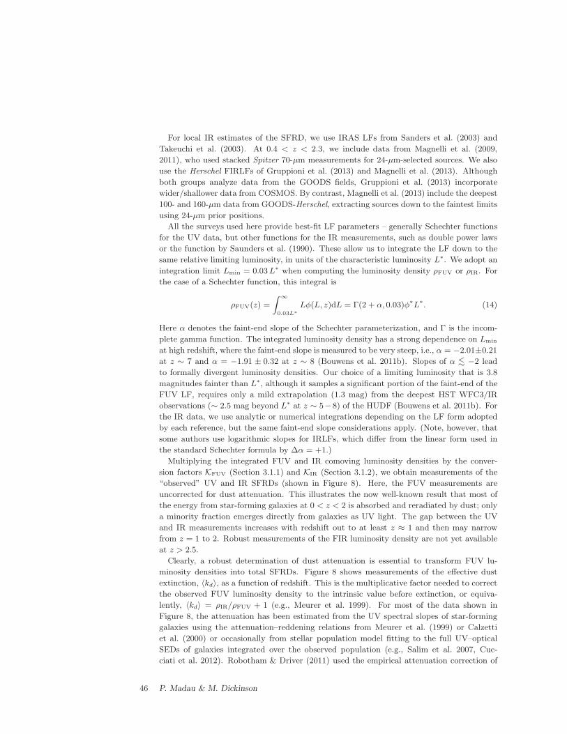
For local IR estimates of the SFRD, we use IRAS LFs from Sanders et al. (2003) and

Takeuchi et al. (2003). At 0.4 < z < 2.3, we include data from Magnelli et al. (2009,

2011), who used stacked Spitzer 70-µm measurements for 24-µm-selected sources. We also

use the Herschel FIRLFs of Gruppioni et al. (2013) and Magnelli et al. (2013). Although

both groups analyze data from the GOODS fields, Gruppioni et al. (2013) incorporate

wider/shallower data from COSMOS. By contrast, Magnelli et al. (2013) include the deepest

100- and 160-µm data from GOODS-Herschel, extracting sources down to the faintest limits

using 24-µm prior positions.

All the surveys used here provide best-fit LF parameters – generally Schechter functions

for the UV data, but other functions for the IR measurements, such as double power laws

or the function by Saunders et al. (1990). These allow us to integrate the LF down to the

same relative limiting luminosity, in units of the characteristic luminosity L∗. We adopt an

integration limit Lmin = 0.03L∗ when computing the luminosity density ρFUV or ρIR. For

the case of a Schechter function, this integral is

ρFUV(z) =

∫ ∞

0.03L∗

Lφ(L, z)dL = Γ(2 + α, 0.03)φ∗L∗. (14)

Here α denotes the faint-end slope of the Schechter parameterization, and Γ is the incom-

plete gamma function. The integrated luminosity density has a strong dependence on Lmin

at high redshift, where the faint-end slope is measured to be very steep, i.e., α = −2.01±0.21

at z ∼ 7 and α = −1.91 ± 0.32 at z ∼ 8 (Bouwens et al. 2011b). Slopes of α ∼< −2 lead

to formally divergent luminosity densities. Our choice of a limiting luminosity that is 3.8

magnitudes fainter than L∗, although it samples a significant portion of the faint-end of the

FUV LF, requires only a mild extrapolation (1.3 mag) from the deepest HST WFC3/IR

observations (∼ 2.5 mag beyond L∗ at z ∼ 5−8) of the HUDF (Bouwens et al. 2011b). For

the IR data, we use analytic or numerical integrations depending on the LF form adopted

by each reference, but the same faint-end slope considerations apply. (Note, however, that

some authors use logarithmic slopes for IRLFs, which differ from the linear form used in

the standard Schechter formula by ∆α = +1.)

Multiplying the integrated FUV and IR comoving luminosity densities by the conver-

sion factors KFUV (Section 3.1.1) and KIR (Section 3.1.2), we obtain measurements of the

“observed” UV and IR SFRDs (shown in Figure 8). Here, the FUV measurements are

uncorrected for dust attenuation. This illustrates the now well-known result that most of

the energy from star-forming galaxies at 0 < z < 2 is absorbed and reradiated by dust; only

a minority fraction emerges directly from galaxies as UV light. The gap between the UV

and IR measurements increases with redshift out to at least z ≈ 1 and then may narrow

from z = 1 to 2. Robust measurements of the FIR luminosity density are not yet available

at z > 2.5.

Clearly, a robust determination of dust attenuation is essential to transform FUV lu-

minosity densities into total SFRDs. Figure 8 shows measurements of the effective dust

extinction, 〈kd〉, as a function of redshift. This is the multiplicative factor needed to correct

the observed FUV luminosity density to the intrinsic value before extinction, or equiva-

lently, 〈kd〉 = ρIR/ρFUV + 1 (e.g., Meurer et al. 1999). For most of the data shown in

Figure 8, the attenuation has been estimated from the UV spectral slopes of star-forming

galaxies using the attenuation–reddening relations from Meurer et al. (1999) or Calzetti

et al. (2000) or occasionally from stellar population model fitting to the full UV–optical

SEDs of galaxies integrated over the observed population (e.g., Salim et al. 2007, Cuc-

ciati et al. 2012). Robotham & Driver (2011) used the empirical attenuation correction of


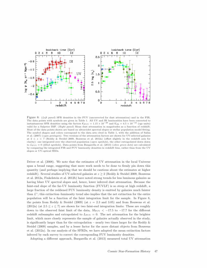
Figure 8: (Left panel) SFR densities in the FUV (uncorrected for dust attenuation) and in the FIR.

The data points with symbols are given in Table 1. All UV and IR luminosities have been converted to

instantaneous SFR densities using the factors KFUV = 1.15 × 10−28 and KIR = 4.5 × 10−44 (cgs units)

valid for a Salpeter IMF. (Right panel) Mean dust attenuation in magnitudes as a function of redshift.

Most of the data points shown are based on ultraviolet spectral slopes or stellar population model fitting.

The symbol shapes and colors correspond to the data sets cited in Table 1, with the addition of Salim

et al. (2007) (cyan pentagon). Two versions of the attenuation factors are shown for UV-selected galaxies

at 2 < z < 7 (Reddy & Steidel 2009, Bouwens et al. 2012a) (offset slightly in the redshift axis for

clarity): one integrated over the observed population (open symbols), the other extrapolated down down

to LFUV = 0 (filled symbols). Data points from Burgarella et al. (2013) (olive green dots) are calculated

by comparing the integrated FIR and FUV luminosity densities in redshift bins, rather than from the UV

slopes or UV-optical SEDs.

Driver et al. (2008). We note that the estimates of UV attenuation in the local Universe

span a broad range, suggesting that more work needs to be done to firmly pin down this

quantity (and perhaps implying that we should be cautious about the estimates at higher

redshift). Several studies of UV-selected galaxies at z ≥ 2 (Reddy & Steidel 2009, Bouwens

et al. 2012a, Finkelstein et al. 2012b) have noted strong trends for less luminous galaxies as

having bluer UV spectral slopes and, hence, lower inferred dust attenuation. Because the

faint-end slope of the far-UV luminosity function (FUVLF) is so steep at high redshift, a

large fraction of the reddened FUV luminosity density is emitted by galaxies much fainter

than L∗; this extinction–luminosity trend also implies that the net extinction for the entire

population will be a function of the faint integration limit for the sample. In Figure 8,

the points from Reddy & Steidel (2009) (at z = 2.3 and 3.05) and from Bouwens et al.

(2012a) (at 2.5 ≤ z ≤ 7) are shown for two faint-end integration limits: These are roughly

down to the observed faint limit of the data, MFUV < −17.5 to −17.7 for the different

redshift subsamples and extrapolated to LFUV = 0. The net attenuation for the brighter

limit, which more closely represents the sample of galaxies actually observed in the study,

is significantly larger than for the extrapolation – nearly two times larger for the Reddy &

Steidel (2009) samples, and by a lesser factor for the more distant objects from Bouwens

et al. (2012a). In our analysis of the SFRDs, we have adopted the mean extinction factors

inferred by each survey to correct the corresponding FUV luminosity densities.

Adopting a different approach, Burgarella et al. (2013) measured total UV attenuation


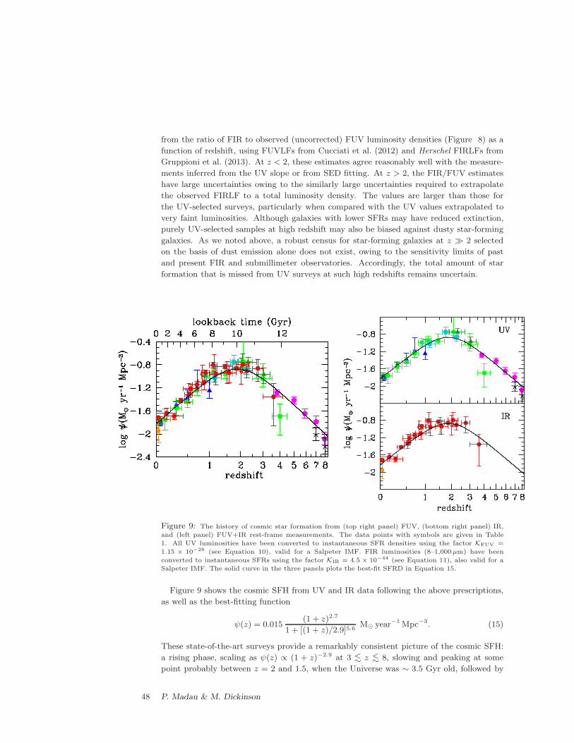
from the ratio of FIR to observed (uncorrected) FUV luminosity densities (Figure 8) as a

function of redshift, using FUVLFs from Cucciati et al. (2012) and Herschel FIRLFs from

Gruppioni et al. (2013). At z < 2, these estimates agree reasonably well with the measure-

ments inferred from the UV slope or from SED fitting. At z > 2, the FIR/FUV estimates

have large uncertainties owing to the similarly large uncertainties required to extrapolate

the observed FIRLF to a total luminosity density. The values are larger than those for

the UV-selected surveys, particularly when compared with the UV values extrapolated to

very faint luminosities. Although galaxies with lower SFRs may have reduced extinction,

purely UV-selected samples at high redshift may also be biased against dusty star-forming

galaxies. As we noted above, a robust census for star-forming galaxies at z ≫ 2 selected

on the basis of dust emission alone does not exist, owing to the sensitivity limits of past

and present FIR and submillimeter observatories. Accordingly, the total amount of star

formation that is missed from UV surveys at such high redshifts remains uncertain.

Figure 9: The history of cosmic star formation from (top right panel) FUV, (bottom right panel) IR,

and (left panel) FUV+IR rest-frame measurements. The data points with symbols are given in Table

1. All UV luminosities have been converted to instantaneous SFR densities using the factor KFUV =

1.15 × 10−28 (see Equation 10), valid for a Salpeter IMF. FIR luminosities (8–1,000µm) have been

converted to instantaneous SFRs using the factor KIR = 4.5 × 10−44 (see Equation 11), also valid for a

Salpeter IMF. The solid curve in the three panels plots the best-fit SFRD in Equation 15.

Figure 9 shows the cosmic SFH from UV and IR data following the above prescriptions,

as well as the best-fitting function

ψ(z) = 0.015(1 + z)2.7

1 + [(1 + z)/2.9]5.6M⊙ year−1 Mpc−3. (15)

These state-of-the-art surveys provide a remarkably consistent picture of the cosmic SFH:

a rising phase, scaling as ψ(z) ∝ (1 + z)−2.9 at 3 ∼< z ∼

< 8, slowing and peaking at some

point probably between z = 2 and 1.5, when the Universe was ∼ 3.5 Gyr old, followed by


a gradual decline to the present day, roughly as ψ(z) ∝ (1 + z)2.7. The comoving SFRD

at redshift 7 was approximately the same as that measured locally. The increase in ψ(z)

from z ≈ 8 to 3 appears to have been steady, with no sharp drop at the highest redshifts,

although there is now active debate in the literature about whether that trend continues

or breaks at redshifts 9 and beyond (Coe et al. 2013, Ellis et al. 2013, Oesch et al. 2013).

Although we have adopted a fitting function that is a double power-law in (1 + z), we note

that the SFRD data at z < 1 can also be fit quite well by an exponential decline with

cosmic time and an e-folding timescale of 3.9 Gyr. Compared with the recent empirical fit

to the SFRD by Behroozi et al. (2013), the function in Equation 15 reaches its peak at a

slightly higher redshift, with a lower maximum value of ψ and with slightly shallower rates

of change at both lower and higher redshift, and produces 20% fewer stars by z = 0.

We also note that each published measurement has its own approach to computing un-

certainties on the SFRD and takes different random and systematic factors into account,

and we have made no attempt to rationalize these here. Moreover, the published studies

integrate their measurements down to different luminosity limits. We have instead adopted

a fixed threshold of 0.03L∗ to integrate the published LFs, and given the covariance on the

measurements and uncertainties of LF parameters, there is no simple way for us to correct

the published uncertainties to be appropriate for our adopted integration limit. Therefore,

we have simply retained the fractional errors on the SFRD measurements published by each

author without modification to provide an indication of the relative inaccuracy derived by

each study. These should not be taken too literally, especially when there is significant dif-

ference in the faint-end slopes of LFs reported in different studies, which can lead to large

differences in the integrated luminosity density. Uncertainties in the faint-end slope and the

resulting extrapolations are not always fully taken into account in published error analyses,

especially when LFs are fit at high redshift by fixing the slope to some value measured only

at lower redshift.

5.2 Core-Collapse Supernova Rate

Because core-collapse supernovae (CC SNe) (i.e., Type II and Ibc SNe) originate from

massive, short-lived stars, the rates of these events should reflect ongoing star formation

and offer an independent determination of the cosmic star formation and metal production

rates at different cosmological epochs (e.g., Madau et al. 1998a, Dahlen et al. 2004). While

poor statistics and dust obscuration are major liming factors for using CC SNe as a tracer

of the SFH of the Universe, most derived rates are consistent with each other and increase

with lookback time between z = 0 and z ∼ 1 (see Figure 10). The comoving volumetric SN

rate is determined by multiplying Equation 15 by the efficiency of forming CC SNe

RCC(z) = ψ(z)×

∫ mmax

mminφ(m)dm

∫ mu

ml

mφ(m)dm≡ ψ(z)× kCC, (16)

where the number of stars that explode as SNe per unit mass is kCC = 0.0068 M−1⊙ for a

Salpeter IMF, mmin = 8 M⊙, and mmax = 40 M⊙. The predicted cosmic SN rate is shown

in Figure 10 and appears to be in good agreement with the data. The IMF dependence in

Equation 16 is largely canceled out by the IMF dependence of the derived SFRD ψ(z), as

the stellar mass range probed by SFR indicators is comparable to the mass range of stars

exploding as CC SNe. Recent comparisons between SFRs and CC SN rates have suggested

a discrepancy between the two rates: The numbers of CC SNe detected are too low by a


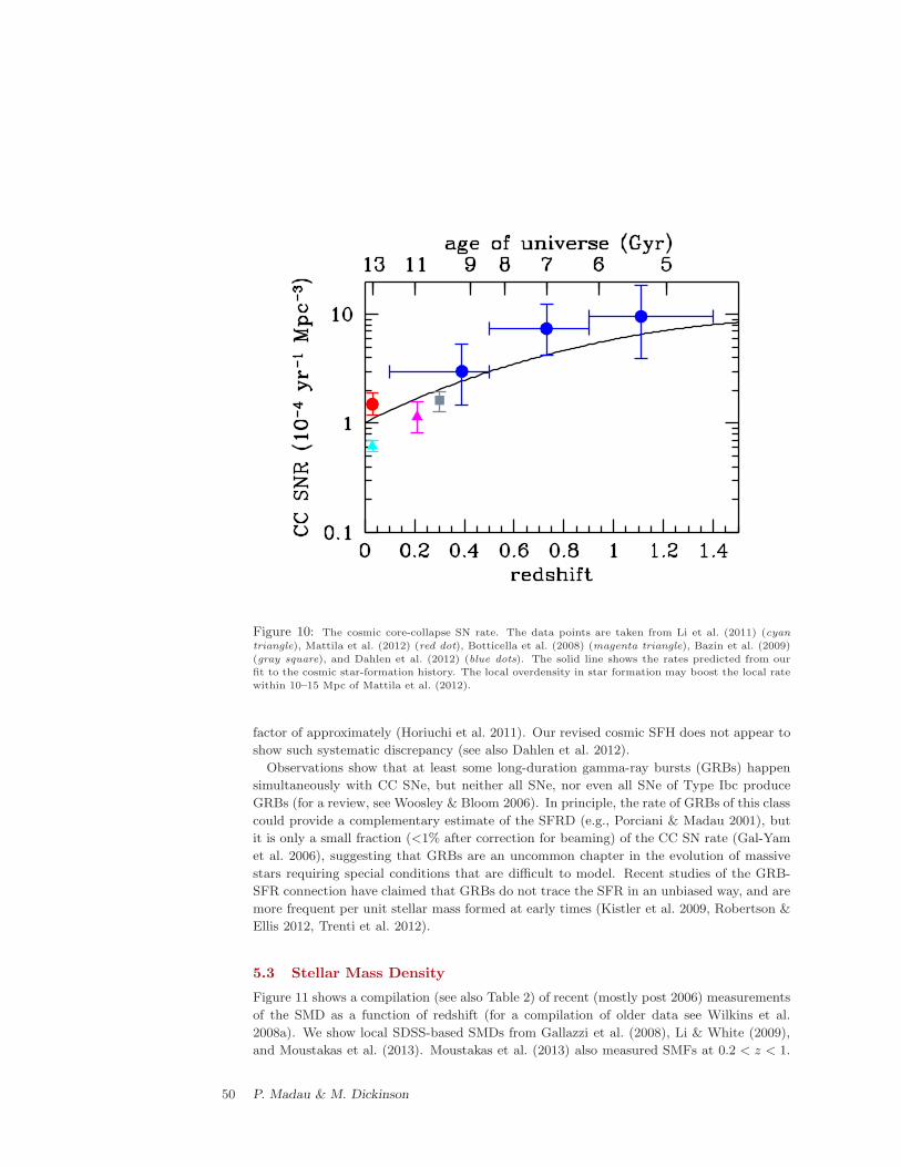
Figure 10: The cosmic core-collapse SN rate. The data points are taken from Li et al. (2011) (cyan

triangle), Mattila et al. (2012) (red dot), Botticella et al. (2008) (magenta triangle), Bazin et al. (2009)

(gray square), and Dahlen et al. (2012) (blue dots). The solid line shows the rates predicted from our

fit to the cosmic star-formation history. The local overdensity in star formation may boost the local rate

within 10–15 Mpc of Mattila et al. (2012).

factor of approximately (Horiuchi et al. 2011). Our revised cosmic SFH does not appear to

show such systematic discrepancy (see also Dahlen et al. 2012).

Observations show that at least some long-duration gamma-ray bursts (GRBs) happen

simultaneously with CC SNe, but neither all SNe, nor even all SNe of Type Ibc produce

GRBs (for a review, see Woosley & Bloom 2006). In principle, the rate of GRBs of this class

could provide a complementary estimate of the SFRD (e.g., Porciani & Madau 2001), but

it is only a small fraction (<1% after correction for beaming) of the CC SN rate (Gal-Yam

et al. 2006), suggesting that GRBs are an uncommon chapter in the evolution of massive

stars requiring special conditions that are difficult to model. Recent studies of the GRB-

SFR connection have claimed that GRBs do not trace the SFR in an unbiased way, and are

more frequent per unit stellar mass formed at early times (Kistler et al. 2009, Robertson &

Ellis 2012, Trenti et al. 2012).

5.3 Stellar Mass Density

Figure 11 shows a compilation (see also Table 2) of recent (mostly post 2006) measurements

of the SMD as a function of redshift (for a compilation of older data see Wilkins et al.

2008a). We show local SDSS-based SMDs from Gallazzi et al. (2008), Li & White (2009),

and Moustakas et al. (2013). Moustakas et al. (2013) also measured SMFs at 0.2 < z < 1.


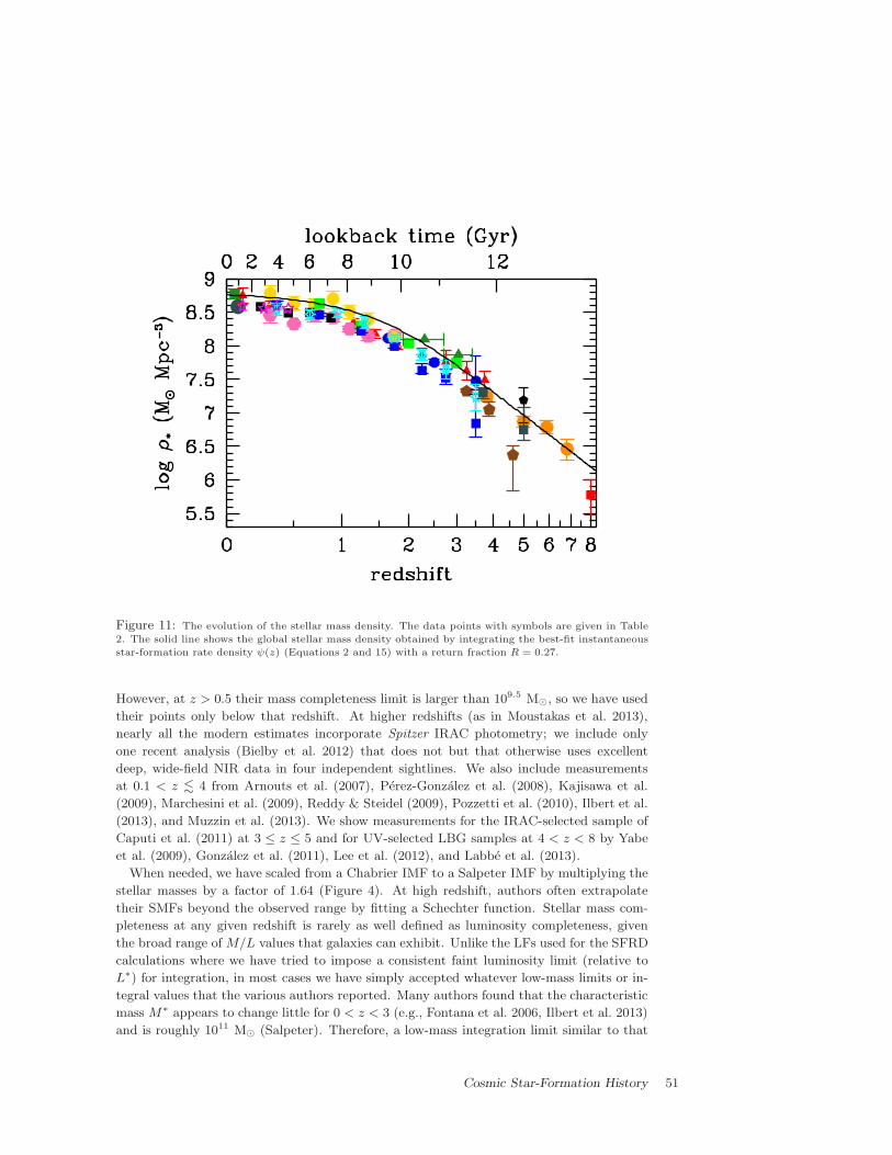
Figure 11: The evolution of the stellar mass density. The data points with symbols are given in Table

2. The solid line shows the global stellar mass density obtained by integrating the best-fit instantaneous

star-formation rate density ψ(z) (Equations 2 and 15) with a return fraction R = 0.27.

However, at z > 0.5 their mass completeness limit is larger than 109.5 M⊙, so we have used

their points only below that redshift. At higher redshifts (as in Moustakas et al. 2013),

nearly all the modern estimates incorporate Spitzer IRAC photometry; we include only

one recent analysis (Bielby et al. 2012) that does not but that otherwise uses excellent

deep, wide-field NIR data in four independent sightlines. We also include measurements

at 0.1 < z ∼< 4 from Arnouts et al. (2007), Perez-Gonzalez et al. (2008), Kajisawa et al.

(2009), Marchesini et al. (2009), Reddy & Steidel (2009), Pozzetti et al. (2010), Ilbert et al.

(2013), and Muzzin et al. (2013). We show measurements for the IRAC-selected sample of

Caputi et al. (2011) at 3 ≤ z ≤ 5 and for UV-selected LBG samples at 4 < z < 8 by Yabe

et al. (2009), Gonzalez et al. (2011), Lee et al. (2012), and Labbe et al. (2013).

When needed, we have scaled from a Chabrier IMF to a Salpeter IMF by multiplying the

stellar masses by a factor of 1.64 (Figure 4). At high redshift, authors often extrapolate

their SMFs beyond the observed range by fitting a Schechter function. Stellar mass com-

pleteness at any given redshift is rarely as well defined as luminosity completeness, given

the broad range ofM/L values that galaxies can exhibit. Unlike the LFs used for the SFRD

calculations where we have tried to impose a consistent faint luminosity limit (relative to

L∗) for integration, in most cases we have simply accepted whatever low-mass limits or in-

tegral values that the various authors reported. Many authors found that the characteristic

mass M∗ appears to change little for 0 < z < 3 (e.g., Fontana et al. 2006, Ilbert et al. 2013)

and is roughly 1011 M⊙ (Salpeter). Therefore, a low-mass integration limit similar to that


which we used for the LFs (Lmin = 0.03L∗) would correspond to Mmin ≈ 109.5 M⊙ in that

redshift range. A common but by no means universal low-mass integration limit used in the

literature is 108 M⊙. Generally, SMFs have flatter low-mass slopes than do UVLFs (and

sometimes IRLFs), so the lower-mass limit makes less difference to the SMDs than it does

to the SFRDs.

Our model predicts an SMD that is somewhat high (∼ 0.2 dex on average, or 60%)

compared with many, but not all, of the data at 0 < z . 3. At 0.2 < z < 2, our

model matches the SMD measurements for the Spitzer IRAC-selected sample of Arnouts

et al. (2007), but several other modern measurements in this redshift range from COSMOS

(Pozzetti et al. 2010, Ilbert et al. 2013, Muzzin et al. 2013) fall below our curve. Carried

down to z = 0, our model is somewhat high compared with several, but not all (Gallazzi

et al. 2008), local estimates of the SMD (e.g., Cole et al. 2001, Baldry et al. 2008, Li &

White 2009).

Several previous analyses (Hopkins & Beacom 2006, but see the erratum; Hopkins &

Beacom 2008; Wilkins et al. 2008a) have found that the instantaneous SFH over-predicts

the SMD by larger factors, up to 0.6 dex at redshift 3. We find little evidence for such

significant discrepancies, although there does appear to be a net offset over a broad redshift

range. Although smaller, a ∼ 60% effect should not be disregarded. One can imagine

several possible causes for this discrepancy; we consider several of them here.

Star formation rates may be overestimated, particularly at high redshift during the peak

era of galaxy growth. For UV-based measurements, a likely culprit may be the luminosity-

weighted dust corrections, which could be too large, although it is often asserted that UV

data are likely to underestimate SFRs in very dusty, luminous galaxies. IR-based SFRs

may be overestimated and indeed were overestimated for some high-redshift galaxies in

earlier Spitzer studies, although this seems less likely now in the era of deep Herschel FIR

measurements. It seems more plausible that the SFRs inferred for individual galaxies may

be correct on average but that the luminosity function extrapolations could be too large.

Many authors adopt fairly steep (α ≥ −1.6) faint-end slopes to both the UVLFs and IRLFs

for distant galaxies. For the UVLFs, the best modern data constrain these slopes quite well,

but in the IR current measurements are not deep enough to do so. However, although these

extrapolations may be uncertain, the good agreement between the current best estimates

of the UV- and IR-based SFRDs at 0 < z < 2.5 (Figure 9) does not clearly point to a

problem in either one.

Instead, stellar masses or their integrated SMD may be systematically underestimated.

This is not implausible, particularly for star-forming galaxies, where the problem of recent

star formation “outshining” older high M/L stars is well known (see Section 5.1). By ana-

lyzing mock catalogs of galaxies drawn from simulations with realistic (and complex) SFHs,

Pforr et al. (2012) found that the simplifying assumptions that are typically made when

modeling stellar masses for real surveys generally lead to systematically underestimated

stellar masses at all redshifts. That said, other systematic effects can work in the opposite

direction and lead to mass overestimates, e.g., the effects of TP-AGB stars on the red and

NIR light if these are not correctly modeled (Maraston 2005). A steeper low-mass slope

to the GSMF could also increase the total SMD. This has been suggested even at z = 0,

where mass functions have been measured with seemingly great precision and dynamic

range (e.g., Baldry et al. 2008). At high redshift, most studies to date have found rela-

tively flat low-mass SMF slopes, but galaxy samples may be incomplete (and photometric

redshift estimates poor) for very faint, red, high-M/L galaxies if they exist in significant

numbers. Some recent SMF determinations using very deep HST WFC3 observations have


found steeper SMF slopes at z > 1.5 (e.g., Santini et al. 2012), and new measurements

from extremely deep NIR surveys such as CANDELS are eagerly anticipated. That said,

it seems unlikely that the SMF slope at low redshift has been underestimated enough to

account for a difference of 0.2 dex in the SMD.

Recent evidence has suggested that strong nebular line emission can significantly affect

broadband photometry for galaxies at high redshift, particularly z > 3.8, where Hα (and,

at z > 5.3, [OIII]) enter the Spitzer IRAC bands (Shim et al. 2011). Therefore, following

Stark et al. (2013), we have divided the SMD of Gonzalez et al. (2011) at z ≃ 4, 5, 6, and

7 in Figure 11 by the factor 1.1, 1.3, 1.6, and 2.4, respectively, to account for this effect.

Although considerable uncertainties in these corrections remain, such downward revision

to the inferred early SMD improves consistency with expectations from the time-integrated

SFRD.

Alternatively, some authors have considered how changing the IMF may help reconcile

SMD(z) with the time-integrated SFRD(z) (e.g., Wilkins et al. 2008b). Generally, a more

top-heavy or bottom-light IMF will lead to larger luminosities per unit SFR, hence smaller

SFR/L conversion factors K (Section 3.1). Mass-to-light ratios for older stellar populations

will also tend to be smaller, but not necessarily by the same factor. Although we have used

a Salpeter IMF for reference in this review, an IMF with a low-mass turnover (e.g., Chabrier

or Kroupa) will yield a larger mass return fraction R and proportionately lower final stellar

masses for a given integrated past SFH, by the factor (1 − R1)/(1 − R2) = 0.81, where

R1 and R2 = 0.41 and 0.27 for the Chabrier and Salpeter IMFs, respectively (Section

2). The apparent offset between the SMD data and our integrated model ψ(z) can be

reduced further to only ∼ 0.1 dex without invoking a particularly unusual IMF. Given the

remaining potential for systemic uncertainties in the measurements of SFRDs and SMDs,

it seems premature to tinker further with the IMF, although if discrepancies remain after

further improvements in the measurements and modeling then this topic may be worth

revisiting.

5.4 Fossil Cosmology

In concordance with estimates from the cosmic SFH, the measurements of the SMD dis-

cussed above imply that galaxies formed the bulk (∼> 75%) of their stellar mass at z < 2.

Stars formed in galaxies before 11.5 Gyr are predicted to contribute only 8% of the to-

tal stellar mass today. An important consistency check for all these determinations could

come from studies of the past SFH of the Universe from its present contents. This “fossil

cosmology” approach has benefited from large spectroscopic surveys in the local Universe

such as the 2dFGRS (Colless et al. 2001) and the SDSS (York et al. 2000), which provide

detailed spectral information for hundreds of thousands of galaxies. Using a sample of

1.7× 105 galaxies drawn from the SDSS DR2, and comparing the spectrum of each galaxy

to a library of templates by Bruzual & Charlot (2003) (the comparison was based on five

spectral absorption features, namely D4,000, Hβ, and HδA + HγA as age-sensitive indexes,

and [Mg2Fe] and [MgFe]’ as metal-sensitive indexes), Gallazzi et al. (2008) have constructed

a distribution of stellar mass as a function of age (for a similar analysis on the SDSS DR3

sample, see also Panter et al. 2007). In Figure 12, we compare this distribution with the

one predicted by our best-fit cosmic SFH. The latter implies a mass-weighted mean stellar

age,

〈tage〉 = t0 −

∫ t0

0

tψ(t)dt

[∫ t0

0

ψ(t)dt

]−1

, (17)


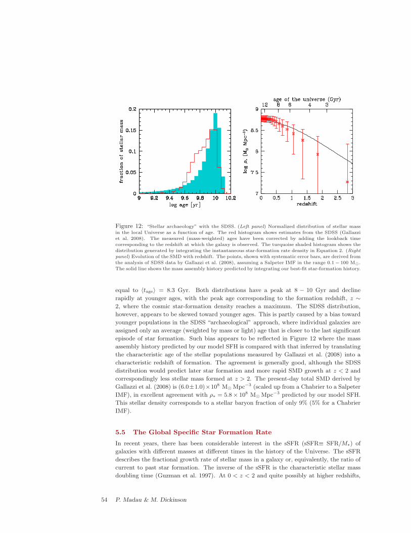
Figure 12: “Stellar archaeology” with the SDSS. (Left panel) Normalized distribution of stellar mass

in the local Universe as a function of age. The red histogram shows estimates from the SDSS (Gallazzi

et al. 2008). The measured (mass-weighted) ages have been corrected by adding the lookback time

corresponding to the redshift at which the galaxy is observed. The turquoise shaded histogram shows the

distribution generated by integrating the instantaneous star-formation rate density in Equation 2. (Right

panel) Evolution of the SMD with redshift. The points, shown with systematic error bars, are derived from

the analysis of SDSS data by Gallazzi et al. (2008), assuming a Salpeter IMF in the range 0.1− 100 M⊙.

The solid line shows the mass assembly history predicted by integrating our best-fit star-formation history.

equal to 〈tage〉 = 8.3 Gyr. Both distributions have a peak at 8 − 10 Gyr and decline

rapidly at younger ages, with the peak age corresponding to the formation redshift, z ∼

2, where the cosmic star-formation density reaches a maximum. The SDSS distribution,

however, appears to be skewed toward younger ages. This is partly caused by a bias toward

younger populations in the SDSS “archaeological” approach, where individual galaxies are

assigned only an average (weighted by mass or light) age that is closer to the last significant

episode of star formation. Such bias appears to be reflected in Figure 12 where the mass

assembly history predicted by our model SFH is compared with that inferred by translating

the characteristic age of the stellar populations measured by Gallazzi et al. (2008) into a

characteristic redshift of formation. The agreement is generally good, although the SDSS

distribution would predict later star formation and more rapid SMD growth at z < 2 and

correspondingly less stellar mass formed at z > 2. The present-day total SMD derived by

Gallazzi et al. (2008) is (6.0±1.0)×108 M⊙ Mpc−3 (scaled up from a Chabrier to a Salpeter

IMF), in excellent agreement with ρ∗ = 5.8× 108 M⊙ Mpc−3 predicted by our model SFH.

This stellar density corresponds to a stellar baryon fraction of only 9% (5% for a Chabrier

IMF).

5.5 The Global Specific Star Formation Rate

In recent years, there has been considerable interest in the sSFR (sSFR≡ SFR/M∗) of

galaxies with different masses at different times in the history of the Universe. The sSFR

describes the fractional growth rate of stellar mass in a galaxy or, equivalently, the ratio of

current to past star formation. The inverse of the sSFR is the characteristic stellar mass

doubling time (Guzman et al. 1997). At 0 < z < 2 and quite possibly at higher redshifts,


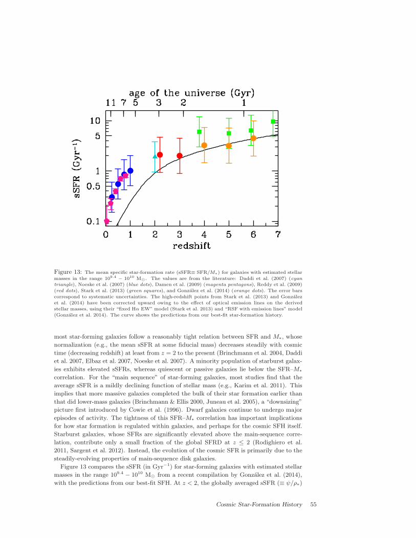
Figure 13: The mean specific star-formation rate (sSFR≡ SFR/M∗) for galaxies with estimated stellar

masses in the range 109.4 − 1010 M⊙. The values are from the literature: Daddi et al. (2007) (cyan

triangle), Noeske et al. (2007) (blue dots), Damen et al. (2009) (magenta pentagons), Reddy et al. (2009)

(red dots), Stark et al. (2013) (green squares), and Gonzalez et al. (2014) (orange dots). The error bars

correspond to systematic uncertainties. The high-redshift points from Stark et al. (2013) and Gonzalez

et al. (2014) have been corrected upward owing to the effect of optical emission lines on the derived

stellar masses, using their “fixed Hα EW” model (Stark et al. 2013) and “RSF with emission lines” model

(Gonzalez et al. 2014). The curve shows the predictions from our best-fit star-formation history.

most star-forming galaxies follow a reasonably tight relation between SFR and M∗, whose

normalization (e.g., the mean sSFR at some fiducial mass) decreases steadily with cosmic

time (decreasing redshift) at least from z = 2 to the present (Brinchmann et al. 2004, Daddi

et al. 2007, Elbaz et al. 2007, Noeske et al. 2007). A minority population of starburst galax-

ies exhibits elevated sSFRs, whereas quiescent or passive galaxies lie below the SFR–M∗

correlation. For the “main sequence” of star-forming galaxies, most studies find that the

average sSFR is a mildly declining function of stellar mass (e.g., Karim et al. 2011). This

implies that more massive galaxies completed the bulk of their star formation earlier than

that did lower-mass galaxies (Brinchmann & Ellis 2000, Juneau et al. 2005), a “downsizing”

picture first introduced by Cowie et al. (1996). Dwarf galaxies continue to undergo major

episodes of activity. The tightness of this SFR–M∗ correlation has important implications

for how star formation is regulated within galaxies, and perhaps for the cosmic SFH itself.

Starburst galaxies, whose SFRs are significantly elevated above the main-sequence corre-

lation, contribute only a small fraction of the global SFRD at z ≤ 2 (Rodighiero et al.

2011, Sargent et al. 2012). Instead, the evolution of the cosmic SFR is primarily due to the

steadily-evolving properties of main-sequence disk galaxies.

Figure 13 compares the sSFR (in Gyr−1) for star-forming galaxies with estimated stellar

masses in the range 109.4 − 1010 M⊙ from a recent compilation by Gonzalez et al. (2014),

with the predictions from our best-fit SFH. At z < 2, the globally averaged sSFR (≡ ψ/ρ∗)


declines more steeply than does that for the star-forming population, as star formation

is “quenched” for an increasingly large fraction of the galaxy population. These passive

galaxies are represented in the global sSFR, but not in the sSFR of the star-forming “main

sequence.” Previous derivations showed a nearly constant sSFR of ∼ 2Gyr−1 for galaxies

in the redshift range 2 < z < 7, suggesting relatively inefficient early star formation and ex-

ponential growth in SFRs and stellar masses with cosmic time. Recent estimates of reduced

stellar masses were derived after correcting for nebular emission in broad bandphotometry

and appear to require some evolution in the high-z sSFR (Stark et al. 2013, Gonzalez et al.

2014). At these epochs, the global sSFR decreases with increasing cosmic time t as sSFR

∼ 4/t Gyr−1, a consequence of the power-law scaling of our SFRD, ψ(t) ∝ t1.9.

5.6 Cosmic Metallicity

According to Equation 4, the sum of the heavy elements stored in stars and in the gas phase

at any given time, Zρg + 〈Z∗〉ρ∗, is equal to the total mass of metals produced over cosmic

history, yρ∗. It can be useful to express this quantity relative to the baryon density,

Zb(z) ≡yρ∗(z)

ρb, (18)

where ρb = 2.77 × 1011Ωbh2 M⊙ Mpc−3. The evolution of the “mean metallicity of the

Universe”, Zb, predicted by our model SFH is plotted in Figure 14. The global metallicity

is Zb ≃ 0.09 (y/Z⊙) solar at the present epoch (note that this is the same value derived

by Madau et al. 1998b). It drops to Zb ≃ 0.01(y/ Z⊙) solar at z = 2.5, i.e., the star-

formation activity we believe to have taken place between the Big Bang and z = 2.5 (2.5

Gyr later) was sufficient to enrich the Universe as a whole to a metallicity of ∼ 1% solar

(for y ≃ Z⊙). Note that the metal production term yρ∗ (and therefore Zb) depends only

weakly on the IMF (at a fixed luminosity density): Salpeter-based mass-to-light ratios are

1.64 times higher than those based on Chabrier. This is counterbalanced by Salpeter-based

net metal yields that are a factor of ∼ 2 lower than those based on Chabrier (see Section

2).

Figure 14 also shows the metallicity of a variety of astrophysical objects at different

epochs. The mass-weighted average stellar metallicity in the local Universe, 〈Z∗(0)〉 =

(1.04 ± 0.14) Z⊙ (Gallazzi et al. 2008), is plotted together with the metallicity of three

different gaseous components of the distant Universe: a) galaxy clusters, the largest bound

objects for which chemical enrichment can be thoroughly studied, and perhaps the best

example in nature of a “closed box”; b) the damped Lyα absorption systems that originate

in galaxies and dominate the neutral-gas content of the Universe; and c) the highly ionized

circumgalactic and intergalactic gas that participates in the cycle of baryons in and out of

galaxies in the early Universe.

The iron mass in clusters is several times larger than could have been produced by

CC SNe if stars formed with a standard IMF, a discrepancy that may indicate an IMF

in clusters that is skewed toward high-mass stars (e.g., Portinari et al. 2004) and/or to

enhanced iron production by Type Ia SNe (e.g., Maoz & Gal-Yam 2004). The damped Lyα

absorption systems are detected in absorption (i.e., have no luminosity bias) and their large

optical depths at the Lyman limit eliminates the need for uncertain ionization corrections

to deduce metal abundances. Their metallicity is determined with the highest confidence

from elements such as O, S, Si, Zn, and Fe and decreases with increasing redshift down to

≈ 1/600 solar to z ∼ 5 (e.g., Rafelski et al. 2012). The enrichment of the circumgalactic


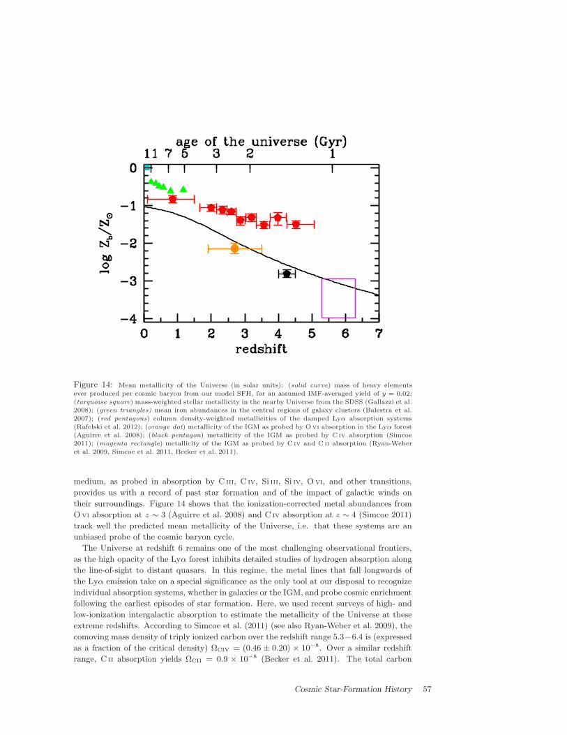
Figure 14: Mean metallicity of the Universe (in solar units): (solid curve) mass of heavy elements

ever produced per cosmic baryon from our model SFH, for an assumed IMF-averaged yield of y = 0.02;

(turquoise square) mass-weighted stellar metallicity in the nearby Universe from the SDSS (Gallazzi et al.

2008); (green triangles) mean iron abundances in the central regions of galaxy clusters (Balestra et al.

2007); (red pentagons) column density-weighted metallicities of the damped Lyα absorption systems

(Rafelski et al. 2012); (orange dot) metallicity of the IGM as probed by OVI absorption in the Lyα forest

(Aguirre et al. 2008); (black pentagon) metallicity of the IGM as probed by C IV absorption (Simcoe

2011); (magenta rectangle) metallicity of the IGM as probed by C IV and C II absorption (Ryan-Weber

et al. 2009, Simcoe et al. 2011, Becker et al. 2011).

medium, as probed in absorption by C III, C IV, Si III, Si IV, OVI, and other transitions,

provides us with a record of past star formation and of the impact of galactic winds on

their surroundings. Figure 14 shows that the ionization-corrected metal abundances from

OVI absorption at z ∼ 3 (Aguirre et al. 2008) and C IV absorption at z ∼ 4 (Simcoe 2011)

track well the predicted mean metallicity of the Universe, i.e. that these systems are an

unbiased probe of the cosmic baryon cycle.

The Universe at redshift 6 remains one of the most challenging observational frontiers,

as the high opacity of the Lyα forest inhibits detailed studies of hydrogen absorption along

the line-of-sight to distant quasars. In this regime, the metal lines that fall longwards of

the Lyα emission take on a special significance as the only tool at our disposal to recognize

individual absorption systems, whether in galaxies or the IGM, and probe cosmic enrichment

following the earliest episodes of star formation. Here, we used recent surveys of high- and

low-ionization intergalactic absorption to estimate the metallicity of the Universe at these

extreme redshifts. According to Simcoe et al. (2011) (see also Ryan-Weber et al. 2009), the

comoving mass density of triply ionized carbon over the redshift range 5.3−6.4 is (expressed

as a fraction of the critical density) ΩCIV = (0.46 ± 0.20) × 10−8. Over a similar redshift

range, C II absorption yields ΩCII = 0.9 × 10−8 (Becker et al. 2011). The total carbon


metallicity by mass, ZC, at 〈z〉 = 5.8 implied by these measurements is

ZC =ΩCIV + ΩCII

Ωb×

C

C II + C IV≃ 3× 10−7 C

C II + C IV, (19)

where (C II + C IV)/C is the fraction of carbon that is either singly or triply ionized. In

Figure 14, we plot ZC in units of the mass fraction of carbon in the Sun, ZC⊙ = 0.003

(Asplund et al. 2009). The lower bound to the rectangle centered at redshift 5.8 assumes

no ionization correction, i.e., (C II +C IV)/C= 1. To derive the upper bound, we adopt the

conservative limit (C II+C IV)/C ≥ 0.1; this is the minimum fractional abundance reached

by C II+C IV under the most favorable photoionization balance conditions at redshift 6. [To

obtain this estimate, we have computed photoionization models based on the CLOUDY

code (Ferland et al. 1998) assuming the UV radiation background at z = 6 of Haardt &

Madau (2012) and a range of gas overdensities 0 < log δ < 3.] If the ionization state of

the early metal-bearing IGM is such that most of the C is either singly or triply ionized,

then most of the heavy elements at these epochs appear to be “missing” compared with

the expectations based on the integral of the cosmic SFH (Ryan-Weber et al. 2009, Pettini

2006). Conversely, if C II and C IV are only trace ion stages of carbon, then the majority

of the heavy elements produced by stars 1 Gyr after the Big Bang (z = 6) may have been

detected already.

A simple argument can also be made against the possibility that our best-fit SFH sig-

nificantly overpredicts the cosmic metallicity at these early epoch. The massive stars that

explode as Type II SNe and seed the IGM with metals are also the sources of nearly all

of the Lyman-continuum (LyC) photons produced by a burst of star formation. It is then

relatively straightforward to link a given IGM metallicity to the minimum number of LyC

photons that must have been produced up until that time. The close correspondence be-

tween the sources of metals and photons makes the conversion from one to the other largely

independent of the details of the stellar IMF (Madau & Shull 1996). Specifically, the energy

emitted in hydrogen ionizing radiation per baryon, Eion, is related to the average cosmic

metallicity by

Eion = ηmpc2Zb, (20)

where mpc2 = 938 MeV is the rest mass of the proton and η is the efficiency of conversion

of the heavy element rest mass into LyC radiation. For stars with Z∗ = Z⊙/50, one derives

η = 0.014 (Schaerer 2002, Venkatesan & Truran 2003). An average energy of 22 eV per LyC

photon together with our prediction of Zb = 7×10−4 Z⊙ (assuming a solar yield) at redshift

6 imply that approximately 8 LyC photons per baryon were emitted by early galaxies prior

to this epoch. Although at least one photon per baryon is needed for reionization to occur,

this is a reasonable value because the effect of hydrogen recombinations in the IGM and

within individual halos will likely boost the number of photons required. A global metallicity

at z = 6 that was much lower than our predicted value would effectively create a deficit

of UV radiation and leave the reionization of the IGM unexplained. In Section 5.8 below

we link the production of LyC photons to stellar mass, show that the efficiency of LyC

production decreases with increasing Z∗, and discuss early star formation and the epoch of

reionization in more detail.

5.7 Black Hole Accretion History

Direct dynamical measurements show that most local massive galaxies host a quiescent

massive black hole in their nuclei. Their masses correlate tightly with the stellar velocity


dispersion of the host stellar bulge, as manifested in the MBH − σ∗ relation of spheroids

(Ferrarese & Merritt 2000, Gebhardt et al. 2000). It is not yet understood whether such

scaling relations were set in primordial structures and maintained throughout cosmic time

with a small dispersion or which physical processes established such correlations in the first

place. Nor it is understood whether the energy released during the luminous quasar phase

has a global impact on the host, generating large-scale galactic outflows and quenching star

formation (Di Matteo et al. 2005), or just modifies gas dynamics in the galactic nucleus

(Debuhr et al. 2010).

Here, we consider a different perspective on the link between the assembly of the stel-

lar component of galaxies and the growth of their central black holes. The cosmic mass

accretion history of massive black holes can be inferred using Soltan’s argument (Soltan

1982), which relates the quasar bolometric luminosity density to the rate at which mass

accumulates into black holes,

ρBH(z) =1− ǫ

ǫc2

∫

Lφ(L, z)dL, (21)

where ǫ is the efficiency of conversion of rest-mass energy into radiation. In practice,

bolometric luminosities are typically derived from observations of the AGN emission at X-

ray, optical or IR wavelengths, scaled by a bolometric correction. In Figure 15, several recent

determinations of the massive black hole mass growth rate are compared with the SFRD

(Equation 15). Also shown is the accretion history derived from the hard X-ray LF of Aird

et al. (2010), assuming a radiative efficiency ǫ = 0.1 and a constant bolometric correction

of 40 for the observed 2-10 KeV X-ray luminosities. This accretion rate peaks at lower

redshift than does the SFRD and declines more rapidly from z ≈ 1 to 0. However, several

authors have discussed the need for luminosity-dependent bolometric corrections, which in

turn can affect the derived accretion history (e.g., Marconi et al. 2004, Hopkins et al. 2007,

Shankar et al. 2009). Moreover, although the hard X-ray LF includes unobscured as well as

moderately obscured sources that may not be identified as AGN at optical wavelengths, it

can miss Compton thick AGN, which may be identified in other ways, particularly using IR

data. Delvecchio et al. (2014) have used deep Herschel and Spitzer survey data in GOODS-S

and COSMOS to identify AGN by SED fitting. This is a potentially powerful method but

depends on reliable decomposition of the IR emission from AGN and star formation.

Black hole mass growth rates derived from the bolometric AGN LFs of Shankar et al.

(2009) and Delvecchio et al. (2014) are also shown in Figure 15. These more closely track

the cosmic SFH, peaking at z ≈ 2, and suggest that star formation and black hole growth

are closely linked at all redshifts (Boyle & Terlevich 1998, Silverman et al. 2008). However,

the differences between accretion histories published in the recent literature would caution

that it is premature to consider this comparison to be definitive.

5.8 First Light and Cosmic Reionization

Fundamental to our understanding of how the Universe evolved to its present state is the

epoch of “first light,” the first billion years after the Big Bang when the collapse of the

earliest baryonic objects – the elementary building blocks for the more massive systems

that formed later – determined the “initial conditions” of the cosmological structure for-

mation process. The reionization in the all-pervading IGM – the transformation of neutral

hydrogen into an ionized state – is a landmark event in the history of the early Universe.

Studies of Lyα absorption in the spectra of distant quasars show that the IGM is highly


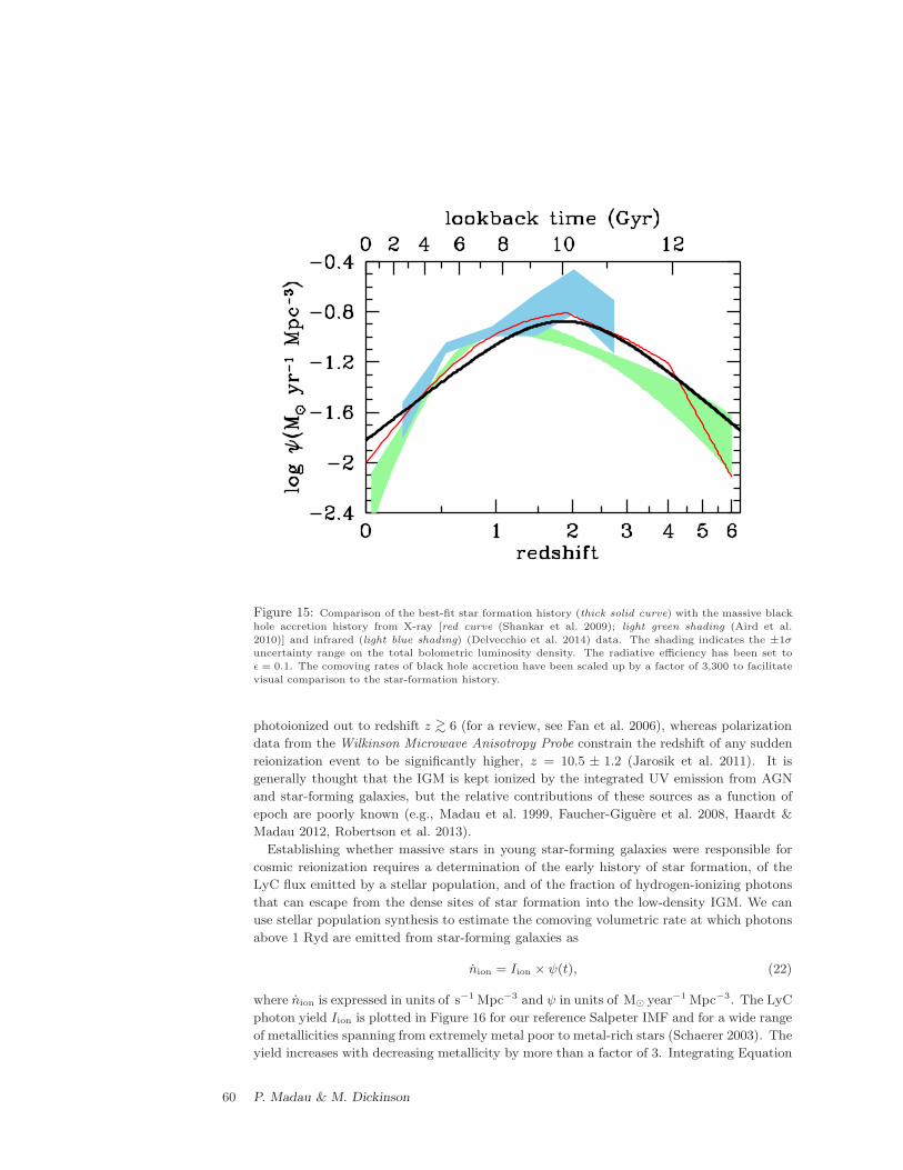
Figure 15: Comparison of the best-fit star formation history (thick solid curve) with the massive black

hole accretion history from X-ray [red curve (Shankar et al. 2009); light green shading (Aird et al.

2010)] and infrared (light blue shading) (Delvecchio et al. 2014) data. The shading indicates the ±1σ

uncertainty range on the total bolometric luminosity density. The radiative efficiency has been set to

ǫ = 0.1. The comoving rates of black hole accretion have been scaled up by a factor of 3,300 to facilitate

visual comparison to the star-formation history.

photoionized out to redshift z ∼> 6 (for a review, see Fan et al. 2006), whereas polarization

data from the Wilkinson Microwave Anisotropy Probe constrain the redshift of any sudden

reionization event to be significantly higher, z = 10.5 ± 1.2 (Jarosik et al. 2011). It is

generally thought that the IGM is kept ionized by the integrated UV emission from AGN

and star-forming galaxies, but the relative contributions of these sources as a function of

epoch are poorly known (e.g., Madau et al. 1999, Faucher-Giguere et al. 2008, Haardt &

Madau 2012, Robertson et al. 2013).

Establishing whether massive stars in young star-forming galaxies were responsible for

cosmic reionization requires a determination of the early history of star formation, of the

LyC flux emitted by a stellar population, and of the fraction of hydrogen-ionizing photons

that can escape from the dense sites of star formation into the low-density IGM. We can

use stellar population synthesis to estimate the comoving volumetric rate at which photons

above 1 Ryd are emitted from star-forming galaxies as

nion = Iion × ψ(t), (22)

where nion is expressed in units of s−1 Mpc−3 and ψ in units of M⊙ year−1 Mpc−3. The LyC

photon yield Iion is plotted in Figure 16 for our reference Salpeter IMF and for a wide range

of metallicities spanning from extremely metal poor to metal-rich stars (Schaerer 2003). The

yield increases with decreasing metallicity by more than a factor of 3. Integrating Equation


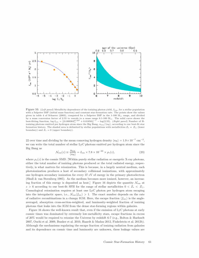
Figure 16: (Left panel) Metallicity dependence of the ionizing photon yield, Iion, for a stellar population

with a Salpeter IMF (initial mass function) and constant star-formation rate. The points show the values

given in table 4 of Schaerer (2003), computed for a Salpeter IMF in the 1-100 M⊙ range, and divided

by a mass conversion factor of 2.55 to rescale to a mass range 0.1-100 M⊙. The solid curve shows the

best-fitting function, log Iion = [(0.00038Z0.227∗ + 0.01858)]−1 − log(2.55). (Right panel) Number of H-

ionizing photons emitted per hydrogen atom since the Big Bang, nion/〈nH〉, according to our best-fit star

formation history. The shaded area is delimited by stellar populations with metallicities Z∗ = Z⊙ (lower

boundary) and Z∗ = 0 (upper boundary).

22 over time and dividing by the mean comoving hydrogen density 〈nH〉 = 1.9×10−7 cm−3,

we can write the total number of stellar LyC photons emitted per hydrogen atom since the

Big Bang as

Nion(z) ≡nion

〈nH〉= Iion × 7.8× 10−60 × ρ∗(z), (23)

where ρ∗(z) is the cosmic SMD. [Within purely stellar radiation or energetic X-ray photons,

either the total number of ionizing photons produced or the total radiated energy, respec-

tively, is what matters for reionization. This is because, in a largely neutral medium, each

photoionization produces a host of secondary collisional ionizations, with approximately

one hydrogen secondary ionization for every 37 eV of energy in the primary photoelectron

(Shull & van Steenberg 1985). As the medium becomes more ionized, however, an increas-

ing fraction of this energy is deposited as heat.] Figure 16 depicts the quantity Nion at

z > 6 according to our best-fit SFH for the range of stellar metallicities 0 < Z∗ < Z⊙.

Cosmological reionization requires at least one LyC photon per hydrogen atom escaping

into the intergalactic space, i.e., Nion〈fesc〉 > 1. The exact number depends on the rate

of radiative recombinations in a clumpy IGM. Here, the escape fraction 〈fesc〉 is the angle-

averaged, absorption cross-section-weighted, and luminosity-weighted fraction of ionizing

photons that leaks into the IGM from the dense star-forming regions within galaxies.

Figure 16 shows the well-known result that, even if the emission of LyC photons at early

cosmic times was dominated by extremely low-metallicity stars, escape fractions in excess

of 20% would be required to reionize the Universe by redshift 6-7 (e.g., Bolton & Haehnelt

2007, Ouchi et al. 2009, Bunker et al. 2010, Haardt & Madau 2012, Finkelstein et al. 2012b).

Although the mechanisms regulating the escape fraction of ionizing radiation from galaxies

and its dependence on cosmic time and luminosity are unknown, these leakage values are


higher than typically inferred from observations of LBGs at z ∼ 3 (e.g., Nestor et al. 2013,

Vanzella et al. 2012, and references therein).

The “reionization budget” is made even tighter by two facts. First, the volume-averaged

hydrogen recombination timescale in the IGM,

〈trec〉 = (χ〈nH〉αB CIGM)−1 ≃ 3.2 Gyr

(

1 + z

7

)−3

C−1IGM, (24)

is ∼60% of the expansion timescale H−1 = H−10 [ΩM (1 + z)3 + ΩΛ]

−1/2 at z = 10, i.e.,

close to two ionizing photon per baryon are needed to keep the IGM ionized. Here, αB

is the recombination coefficient to the excited states of hydrogen, χ = 1.08 accounts for

the presence of photoelectrons from singly ionized helium, and CIGM is the clumping factor

of ionized hydrogen. The above estimate assumes a gas temperature of 2 × 104 K and

a clumping factor for the IGM, CIGM = 1 + 43 z−1.71, that is equal to the clumpiness

of gas below a threshold overdensity of 100 found at z ≥ 6 in a suite of cosmological

hydrodynamical simulations (Pawlik et al. 2009; see also Shull et al. 2012). Second, the

rest-frame UV continuum properties of very high redshift galaxies appear to show little

evidence for the “exotic” stellar populations (e.g., extremely sub-solar metallicities or top-

heavy IMFs) that would significantly boost the LyC photon yield (e.g., Finkelstein et al.

2012a, Dunlop et al. 2013). Although improved knowledge of the SFRD beyond redshift 9

may help to better characterize this photon shortfall, the prospects of a direct observational

determination of the escape fraction of ionizing photons leaking into the IGM at these early

epochs look rather bleak, as the Universe becomes opaque to LyC radiation above redshift

4.

6 CONCLUDING REMARKS

The cosmic history of star formation is one of the most fundamental observables in astro-

physical cosmology. We have reviewed the range of complementary techniques and the-

oretical tools that are allowing astronomers to map the transformation of gas into stars,

the production of heavy elements, and the reionization of the Universe from the cosmic

dark ages to the present epoch. Under the simple assumption of a universal IMF, there

is reasonable agreement between the global SMD inferred at any particular time and the

time integral of all the preceding instantaneous star-formation activity, although modest

offsets may still point toward systematic uncertainties. A consistent picture is emerging,

whereby the SFRD peaked ∼3.5 Gyr after the Big Bang, and dropped exponentially at

z < 1 with an e-folding timescale of 3.9 Gyr. The Universe was a much more active place in

the past: Stars formed at a peak rate approximately nine times higher than is seen today.

Approximately 25% of the present-day SMD formed at z > 2, before the peak of the SFRD,

and another 25% formed since z = 0.7, i.e., roughly over the last half of the Universe’s

age. From the peak of the SFRD at z ≈ 2 to the present day, and perhaps earlier as well,

most stars formed in galaxies that obey a relatively tight SFR–M∗ correlation, and only a

small fraction formed in starbursts with significantly elevated specific SFRs. The smooth

evolution of this dominant main-sequence galaxy population suggests that the evolution of

the cosmic SFH is primarily determined by a balance between gas accretion and feedback

processes, both closely related to galaxy mass, and that stochastic events such as merger-

driven starbursts play a relatively minor role. The growth histories of the stellar component

of galaxies and their central black holes are similar in shape, suggesting broad co-evolution

of black holes and their host galaxies. The rise of the mean metallicity of the Universe to


0.001 solar by redshift six, 1 Gyr after the Big Bang, appears to have been accompanied

by the production of fewer than 10 hydrogen LyC photons per baryon, indicating a rather

tight budget for cosmological reionization. The SFRD at z ≈ 7 was approximately the same

as that of today, at z ≈ 0, but only 1% of today’s SMD was formed during the epoch of

reionization.

As far as the observations and data are concerned, there is still room for improvement

in both SFRD and SMD measurements at virtually every redshift, from the local Universe

to the epoch of reionization (Section 4.6). That said, it would be somewhat surprising

if new measurements changed the picture dramatically at z < 1; it is more likely that

stellar population modeling, e.g., for deriving stellar masses or SFRs, could still change

the details of the picture during the decline and fall of the cosmic SFH. Indeed, at all

redshifts, limitations of our methods for interpreting light as mass may play a significant,

even dominant, role in the error budget for the analyses described in this review. The peak

era of cosmic star formation has been extensively mapped, and yet even with the current

data (Figure 9), it is still hard to accurately pinpoint the redshift of maximum SFRD

within a range ∆z = 1. Our fitting function (Equation 15) places this peak at z ≈ 1.85,

which is plausible but still uncertain. Uncertainties in the faint-end slope of the IRLF

and in extinction corrections for the UVLF still dominate at this peak era of cosmic star

formation. Although evidence seems to point clearly to a steady increase in the SFRD from

z = 8 to z ≈ 2, our direct knowledge of dust-obscured star formation at these redshifts is, for

the most part, limited to the rarest and most ultraluminous galaxies, leaving considerable

uncertainty about how much SFRD we may be missing in the UV census of that early

phase of galaxy evolution. At z > 4, our galaxy surveys have been strongly biased toward

UV-bright galaxies, and may underestimate both SFRDs and SMDs. Even for UV-selected

galaxies, the measurements at z ≥ 8 are very new and likely uncertain, unsupported by

spectroscopic confirmation to date. In addition to measuring redshifts, spectroscopy from

the JWST will help clarify basic issues about nebular line emission and the degree to which

it has affected the photometric analyses that have been carried out to date.

Painstaking though all this vast effort has been, it does miss a crucial point. It says

little about the inner workings of galaxies, i.e., their “metabolism” and the basic process

of ingestion (gas infall and cooling), digestion (star formation), and excretion (outflows).

Ultimately, it also says little about the mapping from dark matter halos to their bary-

onic components. Its roots are in optical-IR astronomy, statistics, stellar populations, and

phenomenology, rather than in the physics of the ISM, self-regulated accretion and star

formation, stellar feedback, and SN-driven galactic winds. It provides a benchmark against

which to compare semi-analytic modeling and hydrodynamical simulations of galaxy for-

mation, but it offers little guidance in identifying the smaller-scale basic mechanisms that

determine the rate of conversion of gas into stars and lead to the grandiose events in the

history of the Universe described in this review.

A variety of physical processes are thought to shape the observed distribution of galaxy

properties, ranging from those responsible for galaxy growth (e.g., star formation and galaxy

merging) to those that regulate such growth (e.g., energetic feedback from SNe, AGN, and

the UV radiation background). However, many of these processes likely depend primar-

ily on the mass of a galaxy’s dark matter halo. Relating the stellar masses and SFRs of

galaxies to the masses and assembly histories of their parent halos is a crucial piece of the

galaxy formation and evolution puzzle. With the accumulation of data from large surveys

and from cosmological numerical simulations, several statistical methods have been devel-

oped over the past decade to link the properties of galaxies to the underlying dark matter


structures (e.g. Berlind & Weinberg 2002, Yang et al. 2003, Vale & Ostriker 2004). One

of them, the “abundance matching” technique, assumes in its simplest form a unique and

monotonic relation between galaxy light and halo mass, and it reproduces galaxy clustering

as a function of luminosity over a wide range in redshift (e.g. Conroy et al. 2006, Guo et al.

2010, Moster et al. 2010). Modern versions of this approach (Moster et al. 2013, Behroozi

et al. 2013) have shown that a) halos of mass ∼ 1012 M⊙ are the most efficient at forming

stars at every epoch, with baryon conversion efficiencies of 20-40% that fall rapidly at both

higher and lower masses; b) in halos similar to that of the Milky Way, approximately half

of the central stellar mass is assembled after redshift 0.7; and c) in low-mass halos, the

accretion of satellites contributes little to the assembly of their central galaxies, whereas in

massive halos more than half of the central stellar mass is formed “ex-situ.” These studies

represent promising advances, albeit with serious potential shortcomings (e.g. Guo & White

2013, Zentner et al. 2013). The assumption of a monotonic relation between stellar mass

and the mass of the host halo is likely incorrect in detail, and it predict only numerically

converged properties on scales that are well resolved in simulations. The matching proce-

dure requires minimal assumptions and avoids an explicit treatment of the physics of galaxy

formation. As such it provides relatively little new insight into this physics. In the version

of this technique by Behroozi et al. (2013), for example, the cosmic SFH is reproduced by

construction.

As of this writing, a solid interpretation of the cosmic SFH from first principles is still

missing (for a recent review, see Mac Low 2013). Generically, one expects that star forma-

tion may be limited at early times by the build-up of dark matter halos and quenched at

low redshift as densities decline from Hubble expansion to the point where gas cooling is

inhibited. These two regimes could then lead to a peak in the SFH at intermediate redshifts

(Hernquist & Springel 2003). A decade ago, hydrodynamical simulations predicted that the

peak in star-formation activity should occur at a much higher redshift, z ∼> 5, than is ac-

tually observed (Springel & Hernquist 2003, Nagamine et al. 2004). Theoretical modeling

has been unable to correctly forecast the evolution of the SFRD because of the large range

of galaxy masses that contribute significantly to cosmic star formation and the difficulty

in following the feedback of energy into the ISM and circumgalactic medium from stellar

radiation, SN explosions, and accreting massive black holes. Gas cooling in an expanding

Universe is an intrinsically unstable process because cooling acts to increase the density of

the gas, which in turn increases the cooling rate. Systems collapsing at low redshift have low

mean densities and long cooling times, whereas systems collapsing at higher redshifts have

higher mean densities and cool catastrophically. Without feedback processes that transfer

energy to the ISM and reheat it, one is faced with the classical overcooling problem – the

unphysical cooling of hot gas in the poorly resolved inner regions of galaxies – and with the

consequent overproduction of stars at early times. And yet, a completely satisfactory treat-

ment of feedback in hydrodynamical simulations that capture large cosmological volumes

remains elusive, as these mechanisms operate on scales too small to be resolved and must

therefore be incorporated via ad-hoc recipes that are too simplistic to capture the complex

subgrid physics involved (e.g., Schaye et al. 2010).

In-depth knowledge of the mechanisms responsible for suppressing star formation in small

halos (e.g., Governato et al. 2010, Krumholz & Dekel 2012, Kuhlen et al. 2012), more pow-

erful supercomputers, better algorithms as well as more robust numerical implementations

of stellar feedback (e.g., Agertz et al. 2013) all now appear as crucial prerequisites for pre-

dicting more realistic SFHs. Newer and deeper observations from the ground and space

should improve our measurements of the galaxy population and its integrated properties,


especially at and beyond the current redshift frontier where data remains sparse. It seems

likely, however, that the most important contribution of new surveys and better modeling

will be toward a detailed understanding of the physics of galaxy evolution, not simply its

demographics.

7 DISCLOSURE STATEMENT

The authors are not aware of any affiliations, memberships, funding, or financial holdings

that might be perceived as affecting the objectivity of this review.

8 ACKNOWLEDGMENTS

This review has benefited from many discussions with and the help of J. Aird, R. Chary,

C. Conroy, O. Cucciati, D. Elbaz, S. Faber, H. Ferguson, A. Gallazzi, V. Gonzalez, A.

Klypin, K.-S. Lee, D. Maoz, P. Oesch, M. Pettini, J. Pforr, L. Pozzetti, J. Primack, J. X.

Prochaska, M. Rafelski, A. Renzini, B. Robertson, M. Schenker, and D. Stark. Support

for this work was provided by the National Science Foundation (NSF) through grant OIA-

1124453, by NASA through grant NNX12AF87G (P.M.), and by NOAO, which is operated

by the Association of Universities for Research in Astronomy, under a cooperative agreement

with the NSF (M.D.).

Literature Cited

Agertz O, Kravtsov AV, Leitner, SN, Gnedin NY 2013. Ap. J. 770:25

Aguirre A, Dow-Hygelund C, Schaye J, Theuns T 2008. Ap. J. 689:851

Aird J, Nandra K, Laird ES, et al. 2010. MNRAS 401:2531

Alavi A, Siana B, Richard J, et al. 2014. Ap. J. 780:143

Appleton PN, Fadda DT, Marleau FR, et al. 2004. Ap. J. Suppl. 154:147

Arnouts S, Schiminovich D, Ilbert O, et al. 2005. Ap. J. Let. 619:L43

Arnouts S, Walcher CJ, Le Fevre O, et al. 2007. Astron. Astrophys. 476:137

Ashby MLN, WillnerSP, Fazio GG, et al. 2013. Ap. J. 679:80

Asplund M, Grevesse N, Sauval AJ, Scott P 2009. Annu. Rev. Astron. Astrophy. 47:481

Atek H, Malkan M, McCarthy P 2010. Ap. J. 723:104

Aussel H, Cesarsky CJ, Elbaz D, Stark JL 1999. Astron. Astrophys. 342:313

Babbedge TSR, Rowan-Robinson M, Vaccari M, et al. 2006. MNRAS 370:1159

Baldry IK, Driver SP, Loveday J, et al. 2012. MNRAS 421:621

Baldry IK, Glazebrook K 2003. Ap. J. 593:258

Baldry IK, Glazebrook K, Driver SP 2008. MNRAS 388:945

Balestra I, Tozzi P, Ettori S, et al. 2007. Astron. Astrophys. 462:429

Barger A, Cowie LL, Richards EA 2000. Astron. J. 119:2092

Barger A, Cowie LL, Sanders DB, et al. 1998. Nature 394:248

Barger A, Wang W-H, Cowie, LL, et al. 2012. Ap. J. 761:89

Bastian N, Covey KR, Meyer MR 2010. Annu. Rev. Astron. Astrophy. 48:339

Basu-Zych AR, Lehmer BD, Hornschemeier AE, et al. 2013. Ap. J. 762:45

Bazin G, Palanque-Delabrouille N, Rich J, et al. 2009. Astron. Astrophys. 499:653

Becker GD, Sargent WLW, Rauch M, Calverley AP 2011. Ap. J. 735:93

Beckwith SVW, Stiavelli M, Koekemoer AM, et al. 2006. Astron. J. 132:1729

Behroozi PS, Wechsler RH, Conroy C 2013. Ap. J. 770:57

Bell EF, MacIntosh DH, Katz N, Weinberg MD 2003. Ap. J. Suppl. 149:289

Berlind AA, Weinberg DH 2002. Ap. J. 575:587


Berta S, Magnelli B, Nordon R, et al. 2011. Astron. Astrophys. 532:A49

Bethermin M, Le Floc’h E, Olbert O, et al. 2012. Astron. Astrophys. 542:A57

Bielby R, Hudelot P, McCracken HJ, et al. 2012. Astron. Astrophys. 545:23

Blumenthal GR, Faber SM, Primack JR, Rees MJ 1984. Nature 311:517

Bolton, JS, Haehnelt MG 2007. MNRAS 382:325

Botticella MT, Riello M, Cappellaro E, et al. 2008. Astron. Astrophys. 479:49

Bouwens RJ, Illingworth GD, Franx M, Ford H 2007. Ap. J. 670:928

Bouwens RJ, Illingworth GD, Labbe I, et al. 2011a. Nature 469:504

Bouwens RJ, Illingworth GD, Oesch PA, et al. 2011b. Ap. J. 737:90

Bouwens RJ, Illingworth GD, Oesch PA, et al. 2012a. Ap. J. 754:83

Bouwens RJ, Illingworth GD, Oesch PA, et al. 2012b. Ap. J. Let. 752:L5

Bowler RAA, Dunlop JS, McLure RJ, et al. 2012. MNRAS 426:2772

Boyle BJ, Terlevich RJ 1998. MNRAS 293:L49

Brammer GB, van Dokkum PG, Franx M, et al. 2012. Ap. J. Suppl. 200:13

Brammer GB, Whitaker KE, van Dokkum PG, et al. 2011. Ap. J. 739:24

Brandt WN, Hasinger G. 2005. Annu. Rev. Astron. Astrophy. 43:827

Brinchmann J, Charlot S, White SDM, et al. 2004. MNRAS 351:1151

Brinchmann J, Ellis RS 2000. Ap. J. Let. 536:L77

Bruzual G, Charlot S 2003. MNRAS 344:1000

Bruzual G, Charlot S, Gonzalez Lopezlira R, et al. 2013. Proc. Int. Astron. Union 295:435

Buat V, Iglesias-Paramo J, Seibert M, et al. 2005. Ap. J. Let. 619:L51

Buat V, Noll S, Burgarella D, et al. 2012. Astron. Astrophys. 545:A141

Budavari T, Szalay AS, Charlot S, et al. 2005. Ap. J. Let. 619:L31

Bunker AJ, Wilkins S, Ellis RS, et al. 2010. MNRAS 409:855

Burgarella D, Buat V, Gruppioni C, et al. 2013. Astron. Astrophys. 554:A70

Calzetti D 2001. Pub. Astron. Soc. Pac. 113:1449

Calzetti D, Armus L, Bohlin RC, et al. 2000. Ap. J. 533:682

Calzetti D, Kennicutt RC, Engelbracht CW, et al. 2007. Ap. J. 666:870

Calzetti D, Kinney AL, Storchi-Bergmann T 1994. Ap. J. 429:582

Caputi KI, Cirasuolo M, Dunlop JS, et al. 2011. MNRAS 413:162

Caputi KI, Dunlop JS, McLure RJ, et al. 2012. Ap. J. 750:20

Caputi KI, Lagache G, Yan L, et al. 2007. Ap. J. 660:97

Carilli CL, Lee N, Capak P, et al. 2008. Ap. J. 689:883

Castellano M, Fontana A, Boutsia K, et al. 2010a. Astron. Astrophys. 511:A20

Castellano M, Fontana A, Paris D, et al. 2010b. Astron. Astrophys. 524:A28

Chabrier G 2003. Pub. Astron. Soc. Pac. 115:763

Chapman SC, Blain AW, Smail I, Ivison RJ 2005. Ap. J. 622:772

Charlot S, Fall SM 2000. Ap. J. 539:718

Chary R-R, & Elbaz, D 2001. Ap. J. 556:562

Chary R-R, Stern D, Eisenhardt P 2005. Ap. J. Let. 635:L5

Chieffi A, Limongi M 2004. Ap. J. 608:405

Coe D, Zitrin A, Carrasco M, et al. 2013. Ap. J. 762:32

Cohen JG 2002. Ap. J. 567:672

Cole S, Lacey CG, Baugh CM, Frenk CS 2000. MNRAS 319:168

Cole S, Nordberg P, Baugh CM, et al. 2001. MNRAS 326:255

Colless M, Dalton G, Maddox S, et al. 2001. MNRAS 328:1039

Condon JJ 1992. Annu. Rev. Astron. Astrophy. 30:575

Condon JJ, Cotton WD, Broderick JJ 2002. Astron. J. 124:675

Connolly AJ, Szalay AS, Dickinson M, Subbarao MU, Brunner RJ 1997. Ap. J. Let. 486:L11

Conroy C 2013. Annu. Rev. Astron. Astrophy. 51:393

Conroy C, Gunn JE, White M 2009. Ap. J. 699:486

Conroy C, van Dokkum PG 2012. Ap. J. 760:71


Conroy C, Wechsler RH, Kravtson AV 2006. Ap. J. 647:201

Conselice CJ, Bluck AF, Buitrago F, et al. 2011. MNRAS 413:80

Cowie LL, Songaila A, & Barger AJ 1999. Astron. J. 118:603

Cowie LL, Songaila A, Hu EM, Cohen JG 1996. Astron. J. 112:839

Cucciati O, Tresse L, Ilbert O, et al. 2012. Astron. Astrophys. 539:31

Curtis-Lake E, McLure RJ, Dunlop JS, et al. 2013. MNRAS 429:302

Daddi E, Cimatti A, Renzini A, et al. 2004. Ap. J. 617:746

Daddi E, Dannerbauer H, Krips M, et al. 2009. Ap. J. Let. 695:L176

Daddi E, Dickinson M, Chary R, et al. 2005. Ap. J. Let. 631:L13.

Daddi E, Dickinson M, Morrison G, et al. 2007b. Ap. J. 670:156

Dahlen T, Mobasher B, Dickinson M, et al. 2007. Ap. J. 654:172

Dahlen T, Strolger L-G, Riess AG, et al. 2004. Ap. J. 613:189

Dahlen T, Strolger L-G, Riess AG, et al. 2012. Ap. J. 757:70

Dale DA, Bendo GJ, Engelbracht CW, et al. 2005. Ap. J. 633:857

Dale DA, Helou G 2002. Ap. J. 576:159

Damen M, Labbe I, Franx M, et al. 2009. Ap. J. 690:937

Davis M, Efstathiou G, Frenk CS, White SDM 1985. Ap. J. 292:371

Debuhr J, Quataert E, Ma C-P, Hopkins P 2010. MNRAS 406:L55

Delvecchio I, Gruppioni C., Pozzi F, et al. 2014. MNRAS 439:2736

Dey A, Soifer BT, Desai V, et al. 2008. Ap. J. 677:943

Dickinson M, Papovich C, Ferguson HC, Budavari T 2003. Ap. J. 587:25

Dickinson M, Stern D, Giavalisco M, et al. 2004. Ap. J. Let. 600:L99

Diemand J, Kuhlen M, Madau P, et al. 2008. Nature 454:735

Di Matteo T, Springel V, Hernquist L 2005. Nature 433:604

Doherty M, Bunker A, Sharp R, et al. 2006. MNRAS 370:331

Driver SP, Popescu CC, Tuffs RJ, et al. 2008. Ap. J. Let. 678:L101

Dubinski J, Carlberg RG 1991. Ap. J. 378:496

Dunlop JS, Rogers AB, McLure RJ, et al. 2013. MNRAS 432:3520

Dunne L, Eales S, Edmunds M, et al. 2000. MNRAS 315:115

Dunne L, Ivison RJ, Maddox S, et al. 2009. MNRAS 394:3

Dyle S, Dunne L, Eales S, et al. 2010. Astron. Astrophys. 518:L10

Eales SA, Raymond G, Roseboom IG, et al. 2010. Astron. Astrophys. 518:L23

Elbaz D, Daddi E, Le Borgne D, et al. 2007. Astron. Astrophys. 468:33

Elbaz D, Dickinson M, Hwang HS, et al. 2011. Astron. Astrophys. 533:119

Elbaz D, Hwang HS, Magnelli B, et al. 2010. Astron. Astrophys. 518:L29

Ellis RS, McLure RJ, Dunlop JS, et al. 2013. Ap. J. Let. 763:L7

Engelbracht CW, Gordon KD, Rieke GH, et al. 2005. Ap. J. Let. 628:L29

Engelbracht CW, Rieke GH, Gordon KD, et al. 2008. Ap. J. 678:804

Eyles LP, Bunker AJ, Ellis RS, et al. 2007. MNRAS 374:910

Faber SM, Willmer CNA, Wolf C, et al. 2007. Ap. J. 665:265

Fan X, Carilli CL, Keating B 2006. Annu. Rev. Astron. Astrophy. 44:415

Faucher-Giguere C-A, Prochaska JX, Lidz A, Hernquist L, Zaldarriaga M 2008. Ap. J. 681:831

Ferland GJ, Korista KT, Verner DA, et al. 1998. Pub. Astron. Soc. Pac. 110:761

Ferrarese L, Merritt D 2000. Ap. J. Let. 539:L9

Finkelstein SL, Papovich C, Dickinson M, et al. 2013. Nature 502: 524

Finkelstein SL, Papovich C, Ryan RE, et al. 2012a. Ap. J. 758:93

Finkelstein SL, Papovich C, Salmon B, et al. 2012b. Ap. J. 756:164

Flores H, Hammaer F, Thuan TX, et al. 1999. Ap. J. 517:148

Fontana A, Donnarumma I, Vanzella E, et al. 2003. Ap. J. Let. 594:L9

Fontana A, Salimbeni S, Grazian A, et al. 2006. Astron. Astrophys. 459:745

Franceschini A, Andreani P, Danese L 1998. MNRAS 296:709

Franx M, Labbe I, Rudnick G, et al. 2003. Ap. J. Let. 587:L79


Fukugita M, Hogan CJ, Peebles PJE 1998. Ap. J. 503:518

Gallazzi A, Brinchmann J, Charlot S, White SDM 2008, MNRAS 383:1439

Gallego J, Zamorano J, Aragon-Salamanca A, Rego M 1995. Ap. J. Let. 455:L1

Gal-Yam A, Ofek EO, Poznanski D, et al. 2006. Ap. J. 639:331

Gavazzi G, Pierini D, Boselli A 1996. Astron. Astrophys. 312:397

Gebhardt K, Bender R, Bower G, et al. 2000. Ap. J. Let. 539:L13

Geha M, Brown TM, Tumlinson J, et al. 2013. Ap. J. 771:29

Giallongo E, D’Odorico S, Fontana A, et al. 1998. Astron. J. 115:2169

Giavalisco M, Dickinson M, Ferguson HC, et al. 2004a. Ap. J. Let. 600:L103

Giavalisco M, Ferguson HC, Koekemoer, et al. 2004b. Ap. J. Let. 600:L93

Gispert R, Lagache G, Puget JL 2000. Astron. Astrophys. 360:1

Glazebrook K, Blake C, Economou F, Lilly S, Colless M 1999. MNRAS 306:843

Goldader JD, Meurer G, Hekcman TM, et al. 2002. Ap. J. 568:651

Gonzalez V, Bouwens R, Illingworth G, et al. 2014. Ap. J. 781:34

Gonzalez V, Labbe I, Bouwens RJ, et al. 2011. Ap. J. Let. 735:L34

Goto T, Arnouts S, Inami H, et al. 2011a. MNRAS 410:573

Goto T, Arnouts S, Malkan M, et al. 2011b MNRAS 414:1903

Governato F, Brook C, Mayer L, et al. 2010. Nature 463:203

Grazian A, Cstellano M, Koekemoer AM, et al. 2011. Astron. Astrophys. 532:33

Grogin NA, Kocevski DD, Faber SM, Ferguson HC, et al. 2011. Ap. J. Suppl. 197:35

Gruppioni C, Pozzi F, Andreani P, et al. 2010. Astron. Astrophys. 518:L27

Gruppioni C, Pozzi F, Rodighiero G, et al. 2013. MNRAS 432:23

Guedes J, Callegari S, Madau P, Mayer L 2011. Ap. J. 742:76

Gunawardhana MLP, Hopkins AM, Bland-Hawthorn J, et al. 2013. MNRAS 433:2764

Guo Q, White S 2013. MNRAS 437:3228

Guo Q, White S, Li C, Boylan-Kolchin M 2010. MNRAS 404:1111

Guzman R, Gallego J, Koo DC, et al. 1997. Ap. J. 489:559

Jarosik N, Bennett CL, Dunkley J, et al. 2011. Ap. J. Suppl. 192:14

Haardt F, Madau P 2012. Ap. J. 746:125

Haarsma DB, Partridge RB, Windhorst RA, Richards EA 2000. Ap. J. 544:641

Hathi NP, Ryan RE, Cohen SH, et al. 2010. Ap. J. 720:1708

Hayes M, Schaerer D, Ostlin G 2010. Astron. Astrophys. 509:L5

Hernquist L, Springel V 2003. MNRAS 341: 1253

Hirschi R, Meynet G, Maeder A 2005. Astron. Astrophys. 433:1013

Hogg DW, Cohen JG, Blandford R, Pahre MA 1998. Ap. J. 504:622

Hopkins AM 2004. Ap. J. 615:209

Hopkins AM, Beacom JF 2006. Ap. J. 651:142

Hopkins AM, Beacom JF 2008. Ap. J. 682:1486

Hopkins AM, Connolly AJ, Szalay AS 2000. Astron. J. 120:2843

Hopkins PF, Quataert E, Murray N 2012. MNRAS 421:3522

Hopkins PF, Richards GT, Hernquist L 2007. Ap. J. 654:731

Horiuchi S, Beacom JF, Kochanek CS, et al. 2011. Ap. J. 738:154

Huang J-S, Zheng XZ, Rigopoulou D, et al. 2011. Ap. J. 742:L13

Hughes DH, Serjeant S, Dunlop J, et al. 1998. Nature 394:241

Huynh MT, Frayer DT, Mobasher M, et al. 2007. Ap. J. Let. 667:L9

Ilbert O, McCracken HJ, Le Fevre O, et al. 2013. Astron. Astrophys. 556:A55

Ilbert O, Salvato M, Le Floc’h E, et al. 2010. Ap. J. 709:644

Ivison RJ, Alexander DM, Biggs AD, et al. 2010. MNRAS 402:245

Ivison RJ, Magnelli B, Ibar E, et al. 2010. Astron. Astrophys. 518:L31

Iwata I, Ohta K, Tamura N 2007. MNRAS 376:1557

Jarvis M 2012. The VISTA Deep Extragalactic Observations (VIDEO) Survey. Presented at Sci.

Next Gener. Imaging Spectrosc. Surv., ESO Garching, 15-18 October.


Juneau S, Glazebrook K, Crampton D, et al. 2005. Ap. J. Let. 619:L135

Kajisawa M, Ichikawa T, Tanaka I, et al. 2009. Ap. J. 702:1393

Karim A, Schinnerer E, Martınez-Sansigre A, et al. 2011. Ap. J. 730:61

Katz N, Weinberg DH, Hernquist L 1996. Ap. J. Suppl. 105:19

Kauffmann G, Heckman TM, White SDM, et al. 2003. MNRAS 341:33

Kauffmann G, White SDM, Guiderdoni B 1993. MNRAS 264:201

Kennicutt RC 1998. Annu. Rev. Astron. Astrophy. 36:189

Kennicutt RC, & Evans NJ 2012. Annu. Rev. Astron. Astrophy. 50:531

Keres D, Katz N, Weinberg DH, Dave R 2005. MNRAS 363:2

Kewley, L., & Kobulnicky, H. A. 2007. Island Universes: Structure and Evolution of Disk Galaxies,

ed. RS de Jong. Dordrecht: Springer

Kistler M, Yuksel H, Beacom JF, Hopkins AM, Wyithe JSB 2009. Ap. J. 705:104

Klypin A, Trujillo-Gomez S, Primack J 2011. Ap. J. 740:102

Koekemoer AM, Faber SM, Ferguson, HC 2011. Ap. J. Suppl. 197:36

Kong X, Charlot S, Brinchmann J, Fall SM 2004. MNRAS 349:769

Kroupa P 2001. MNRAS 322:231

Krumholz MR, Dekel A 2012. Ap. J. 753:16

Kuhlen M, Krumholz MR, Madau P, Smith B, Wise J. 2012, Ap. J. 749:36

Labbe I, Oesch PA, Bouwens RJ, et al. 2013. Ap. J. Let. 777:L19

Lagache G, Puget J-L, Dole H 2005. Annu. Rev. Astron. Astrophy. 43:727

Laird ES, Nandra K, Adelberger KL, et al. 2005. MNRAS 359:47

Laird ES, Nandra K, Hobbs A, et al. 2006. MNRAS 373:217

Lanzetta KM, Wolfe AM, Turnshek DA 1995. Ap. J. 440:435

Lapi A, Gonzalez-Nuevo J, Fan L, et al. 2011. Ap. J. 742:24

Lawrence A, Walker D, Rowan-Robinson M, Leech KJ, Penston MV 1986. MNRAS 219:687

Lee K-S, Ferguson HC, Wiklind T, et al. 2012. Ap. J. 752:66

Le Floc’h E, Papovich C, Dole H, et al. 2005. Ap. J. 632:169

Lehmer BD, Brandt WN, Alexander DM, et al. 2005. Astron. J. 129:1

Leitherer C, Schaerer D, Goldader JD, et al. 1999. Ap. J. Suppl. 123:3

Li C, White, SDM 2009. MNRAS 398:2177

Li W, Chornock R, Leaman J, et al. 2011. MNRAS 412:1473

Lilly SJ, Le Fevre O, Hammer F, Crampton D 1996. Ap. J. Let. 460:L1

Lonsdale Persson CJ, & Helou G 1987. Ap. J. 314:513

Lorenzoni S, Bunker AJ, Wilkins SM, et al. 2013. MNRAS 429:150

Lutz D 2014. Annu. Rev. Astron. Astrophy. submitted.

Ly C, Lee JC, Dale DA, et al. 2011. Ap. J. 726:109

Ly C, Malkan MA, Kashikawa N et al. 2007. Ap. J. 657:738

Machalski J, Godlowski W 2000. Astron. Astrophys. 360:463

Mac Low M-M 2013. Science 340:6140

Madau P, Della Valle M, Panagia N 1998. MNRAS 297:L17

Madau P, Ferguson HC, Dickinson ME, et al. 1996. MNRAS 283:1388

Madau P, Haardt F, Rees MJ 1999. Ap. J. 514:648

Madau P, Pozzetti L, Dickinson M 1998. Ap. J. 498:106

Madau P, Shull JM 1996. Ap. J. 457:551

Maeder A 1992. Astron. Astrophys. 264:105

Magdis GE, Daddi E, Bethermin M, et al. 2012. Ap. J. 760:6

Magdis GE, Elbaz D, Daddi E, et al. 2010. Ap. J. 714:1740

Magnelli B, Elbaz D, Chary RR, et al. 2009. Astron. Astrophys. 496:57

Magnelli B, Elbaz D, Chary RR, et al. 2011. Astron. Astrophys. 528:A35

Magnelli B, Popesso P, Berta S, et al. 2013. Astron. Astrophys. 553:A132

Mancini C, Matute I, Cimatti A, et al. 2009. Astron. Astrophys. 500:705

Mao MY, Huynh MT, Norris RP, et al. 2011. Ap. J. 731:79


Maoz D, Gal-Yam A 2004. MNRAS 347:951

Maraston C 2005. MNRAS 362:799

Maraston C, Daddi E, Renzini A, et al. 2006. Ap. J. 652:85

Maraston C, Pforr J, Renzini A, et al. 2010. MNRAS 407:830

Marchesini D, van Dokkum PG, Forster Schreiber NM, et al. 2009. Ap. J. 701:1765

Marchesini D, Whitaker KE, Brammer G, et al. 2010. Ap. J. 725:1277

Marconi A, Risaliti G, Gilli R, et al. 2004. MNRAS 351:169

Mattila S, Dahlen T, Efstathiou A, et al. 2012. Ap. J. 756:111

Mauch T, Sadler EM 2007. MNRAS 375:931

Mauduit J-C, Lacy M, Farrah D, et al. 2012. Pub. Astron. Soc. Pac. 124:714

McLure RJ, Cirasuolo M, Dunlop JS, et al. 2009. MNRAS 395:2196

McLure RJ, Dunlop JS, Bowler RAA, et al. 2013. MNRAS 432:2696

Meurer GR, Heckman TM, Calzetti D 1999. Ap. J. 521:64

Moore B, Ghigna S, Governato F, et al. 1999. Ap. J. Let. 524:L19

Moster BP, Naab, T, White, SDM 2013. MNRAS 428:3121

Moster BP, Somerville RS, Maulbetsch C, et al. 2010. Ap. J. 710:903

Moustakas J, Coil A, Aird J, et al. 2013. Ap. J. 767:50

Moustakas J, Kennicutt RC, Tremonti CA 2006. Ap. J. 642:775

Murphy EJ, Condon JJ, Schinnerer E, et al. 2011. Ap. J. 737:67

Muzzin A, Marchesini D, Stefanon M, et al. 2013. Ap. J. 777:18

Nagamine K, Cen R, Hernquist L, Ostriker JP, Springel V 2004, Ap. J. 610:45

Navarro JF, Steinmetz M 2000. Ap. J. 538:477

Nestor DB, Shapley AE, Kornei KA, Steidel CC, Siana B 2013. Ap. J. 765:47

Noeske KG, Faber SM, Weiner BJ, et al. 2007. Ap. J. Let. 660:L47

Nonino M, Dickinson M, Rosati P, et al. 2009. Ap. J. Suppl. 183:244

Nordon R, Lutz D, Shao L, et al. 2010. Astron. Astrophys. 518:L24

Ocvirk P, Pichon C, Teyssier R 2008. MNRAS 390:1326

Oesch PA, Bouwens RJ, Carollo CM, et al. 2010. Ap. J. Let. 725:L150

Oesch PA, Bouwens RJ, Illingworth GD, et al. 2012. Ap. J. 759:135

Oesch PA, Bouwens RJ, Illingworth GD, et al. 2013. Ap. J. 773:75

Ouchi M, Mobasher B, Shimasaku K, et al. 2009. Ap. J. 706:1136

Ouchi M, Shimasaku K, Okamura S, et al. 2004. Ap. J. 611:660

Overzier RA, Heckman TM, Wang J, et al. 2011. Ap. J. Let. 726:L7

Panter B, Jimenez R, Heavens AF, Charlot S 2007. MNRAS 378:1550

Papovich C, Dickinson M, & Ferguson HC 2001. Ap. J. 559:620

Papovich C, Rudnick G, Le Floc’h E, et al. 2007. Ap. J. 668:45

Pascarelle SM, Lanzetta KM, Fernndez-Soto A 1998. Ap. J. Let. 508:L1

Pawlik AH, Schaye J, van Scherpenzeel E 2009. MNRAS 394:4

Patel H, Clements DL, Vaccari M, et al. 2013. MNRAS : 428:291

Peebles PJE 1982. Ap. J. Let. 263:L1

Pei YC, Fall SM 1995. Ap. J. 454:69

Pei YC, Fall SM, Hauser MG 1999. Ap. J. 522:604

Penner K, Dickinson M, Pope A, et al. 2012. Ap. J. 759:28

Perez-Gonzalez PG, Rieke GH, Egami E, et al. 2005. Ap. J. 630:82

Perez-Gonzalez PG, Rieke GH, Villar V, et al. 2008. Ap. J. 675:234

Persic M, Rephaeli Y, Braito V, et al. 2004. Astron. Astrophys. 419:849

Persic M, Salucci P, 1992. MNRAS 258:14

Pettini M 2006. In The Fabulous Destiny of Galaxies: Bridging Past and Present, ed. V LeBrun,

A Mazure, S Arnouts, D Burgarella, pp. 319-335. Paris: Frontiers Group

Pforr J, Maraston C, Tonini C 2012. MNRAS 422:3285

Pope A, Bussmann RS, Dey A, et al. 2008. Ap. J. 689:127

Porciani C, Madau P 2001. Ap. J. 548:522


Portinari L, Moretti A, Chiosi C, Sommer-Larsen J 2004. Ap. J. 604:579

Pozzetti L, Bolzonella M, Zucca E, et al. 2010. Astron. Astrophys. 523:A13

Rafelski M, Wolfe AM, Prochaska JX, Neeleman M, Mendez AJ 2012. Ap. J. 755:89

Raiter A, Fosbury RAE, Teimoorinia H 2010. Astron. Astrophys. 510:A109

Ranalli P, Comastri A, Setti G 2003. Astron. Astrophys. 399:39

Reddy NA, Dickinson M, Elbaz D, et al. 2012. Ap. J. 744:154

Reddy NA, Erb DK, Pettini M, et al. 2010. Ap. J. 712:1070

Reddy NA, Steidel CC 2004. Ap. J. Let. 603:L13

Reddy NA, Steidel CC 2009. Ap. J. 692:778

Reddy NA, Steidel CC, Fadda D, et al. 2006. Ap. J. 744:792

Reddy NA, Steidel CC, Pettini M, et al. 2008. Ap. J. Suppl. 175:48

Retzlaff J, Rosati P, Dickinson M, et al. 2010. Astron. Astrophys. 511:A50

Riechers DA, Bradford CM, Clements DL, et al. 2013. Nature 496:329

Robertson BE, Ellis RS 2012. Ap. J. 744:95

Robertson BE, Furlanetto SR, Schneider E, et al. 2013. Ap. J. 768:71

Robotham ASG, Driver SP 2011. MNRAS 413:2570

Rodighiero G, Cimatti A, Gruppioni C, et al. 2010. Astron. Astrophys. 518:25

Rodighiero G, Daddi E, Baronchelli I, et al. 2011. Ap. J. Let. 739:L40

Rowan-Robinson M, Mann RG, Oliver SJ, et al. 1997. MNRAS 289:490

Rudnick, G, Rix, H-W, Franx M, et al. 2003, Ap. J. 599:847

Rujopakarn W, Eisenstein DJ, Rieke GH, et al. 2010. Ap. J. 718:1171

Rush B, Malkan MA, Spinoglio L 1993. Ap. J. Suppl. 89:1

Ryan-Weber EV, Pettini M, Madau P, Zych B 2009. MNRAS 395:1476

Sadler EM, Jackson CA, Cannon RD 2002. MNRAS 329:227

Salim S, Dickinson M, Rich RM, et al. 2009. Ap. J. 700:161

Salim S, Rich RM, Charlot S, et al. 2007. Ap. J. Suppl. 173:267

Salucci P, Persic M 1999. MNRAS 309:923

Salpeter EE 1955. Ap. J. 121:161

Sanders DB, Mazzarella JM, Kim DC, Surace JA, Soifer BT 2003. Astron. J. 126:1607

Santini, P, Fontana A, Grazian A, et al. 2012. Astron. Astrophys. 538:A33

Sargent MT, Bethermin M, Daddi E, Elbaz D 2012. Ap. J. Let. 747:L31

Sargent MT, Schinnerer E, Murphy E, et al. 2010a. Ap. J. Suppl. 186:341

Sargent MT, Schinnerer E, Murphy E, et al. 2010b. Ap. J. Let. 714:L190

Saunders W, Rowan-Robinson M, Lawrence A., et al. 1990. MNRAS 242:318

Sawicki M, Yee HKC 1998. Astron. J. 115: 1329

Schaerer D 2002. Astron. Astrophys. 382:28

Schaerer D 2003. Astron. Astrophys. 397:527

Schaller G, Schaerer D, Meynet G, Maeder A 1992. Astron. Astrophys. 96:269

Schaye J, Dalla Vecchia C, Booth CM, et al. 2010. MNRAS 402:1536

Schenker MA, Robertson BE, Ellis RS, et al. 2013. Ap. J. , 768:196

Schiminovich D, Ilbert O, Arnouts S, et al. 2005. Ap. J. Let. 619:L47

Sedgwick C, Serjeant S, Pearson C, et al. 2011, MNRAS 416:1862

Serjeant S, Carraminana A, Gonzales-Solares E, et al. 2004. MNRAS 355:813

Serjeant S, Gruppioni C, Oliver S 2002. MNRAS 330:621

Seymour N, Dwelly T, Moss D, et al. 2008. MNRAS 386:1695

Shankar F, Weinberg DH, Miralda-Escude J 2009. Ap. J. 690:20

Shapley A, Steidel CC, Adelberger KL 2001. Ap. J. 562:95

Shim H, Colbert J, Teplitz H, et al. 2009. Ap. J. 696:785

Shim H, Chary RR, Dickinson M, et al. 2011. Ap. J. 738:69

Shull JM, Harness A, Trenti M, Smith BD 2012. Ap. J. 747:100

Shull JM, van Steenberg ME 1985. Ap. J. 298:268

Shupe DL, Fang F, Hacking PB, Huchra JP 1998. Ap. J. 501:597


Silverman JD, Green PJ, Barkhouse WA, et al. 2008. Ap. J. 679:118

Simcoe RA 2011. Ap. J. 738:159

Simcoe RA, Cooksey KL, Matejek M, et al. 2011. Ap. J. 743:21

Smail I, Ivison RJ, Blain AW 1997. Ap. J. Let. 490:L5

Smith JDT, Draine BT, Dale DA, et al. 2007. Ap. J. 656:770

Smolcic V, Schinnerer E, Zamorani G, et al. 2009. Ap. J. 690:610

Sobral D, Best PN, Smail I, et al. 2013. MNRAS 428:1128

Sodriski TJ, Odegard N, Arendt RG, et al. 1997. Ap. J. 480:173

Soifer BT, Sanders DB, Madore BF, et al. 1987. Ap. J. 320:238

Soltan A 1982. MNRAS 200:115

Somerville RS, Primack JR 1999. MNRAS 310:1087

Springel V, Hernquist L 2003. MNRAS 339:289

Springel V, Wang J, Vogelsberger M, et al. 2008. MNRAS 391:1685

Springel V, White SDM, Jenkins A, et al. 2005. Nature 435:629

Stadel J, Potter D, Moore B, et al. 2009. MNRAS 398:L21

Stanway ER, Bunker AJ, McMahon RG 2003. MNRAS 342:439

Stark DP, Bunker A, Ellis RS, et al. 2007. Ap. J. 659:84

Stark DP, Ellis RS, Bunker A, et al. 2009. Ap. J. 697:1493

Stark DP, Schenker MA, Ellis RS, et al. 2013. Ap. J. 763:129

Steidel CC, Adelberger KL, Giavalisco M, Dickinson M, Pettini M 1999. Ap. J. 519:1

Steidel CC, Adelberger KL, Shapley AE, Pettini M, Dickinson M 2003. Ap. J. 592:728

Steidel CC, Giavalisco, M, Pettini M, Dickinson M, Adelberger, KL 1996. Ap. J. Let. 462:L17

Steidel CC, Shapley AE, Pettini M, et al. 2004. Ap. J. 604:534

Steidel CC, Pettini M, Hamilton D 1995. Astron. J. 110:2519

Sullivan M, Treyer MA, Ellis RS, et al. 2000. MNRAS 312:442

Takeuchi TT, Ishii TT, Dole H, et al. 2006. Astron. Astrophys. 448:525

Takeuchi TT, Yoshikawa K, Ishii TT 2003. Ap. J. Let. 587:L89

Thompson RI, Eisenstein D, Fan X, et al. 2006. Ap. J. 647:787

Tilvi V, Papovich C, Tran, KVH, et al. 2013. Ap. J. 768:56

Tinsley BM 1980. Fundam. Cosmic Phys. 5:287

Trenti M, Perna R, Levesque EM, Shull JM, Stocke JT 2012. Ap. J. Let. 749:L38

Tresse L, Ilbert O, Zucca E, et al. 2007. Astron. Astrophys. 472:403

Tresse L, Maddox SJ 1998. Ap. J. 495:691

Tresse L, Maddox SJ, Le Fevre O, Cuby J-G 2002. MNRAS 337:369

Treyer M, Ellis RS, Milliard B, Donas J, Bridges TJ 1998. MNRAS 300:303

Vaccari M, Marchetti L, Franceschini A, et al. 2010. Astron. Astrophys. 518:L20

Vale A, Ostriker JP 2004. MNRAS 353:189

Vanzella E, Guo Y, Giavalisco M, et al. 2012. Ap. J. 751:70

Venkatesan A, Truran JW 2003. Ap. J. Let. 594:L1

Verma A, Lehnert MD, Forster Schreiber NM, et al. 2007. MNRAS 377:1024

Wang W-H, Cowie LL, Barger AJ, et al. 2010. Ap. J. Suppl. 187:251

Wardlow JL, Smail I, Coppin KEK, et al. 2011. MNRAS 415:1479

Weidemann V 2000. Astron. Astrophys. 363:647

Westra E, Geller MJ, Kurtz MJ, Fabricant DG, Dell’Antonio I 2010. Ap. J. 708:534

White SDM, Frenk CS 1991. Ap. J. 379:52

White SDM, Rees MJ 1978. MNRAS 183:341

Wiklind T, Dickinson M, Ferguson HC, et al. 2008. Ap. J. 676:781

Wilkins SM, Hopkins AM, Trentham N, Tojeiro R 2008b. MNRAS 391:363

Wilkins SM, Trentham N, Hopkins AM 2008. MNRAS 385:687

Wilson G, Cowie LL, Barger AJ, Burke DJ 2002. Astron. J. 124:1258

Wolf C, Bell EF, McIntosh DH, et al. 2005. Ap. J. 630:771

Woosley SE, Bloom JS 2006. Annu. Rev. Astron. Astrophy. 44:507


Wyder TK, Treyer MA, Milliard B, et al. 2005. Ap. J. Let. 619:L15

Yabe K, Ohta K, Iwata I, et al. 2009. Ap. J. 693:507

Yan H, Dickinson M, Giavalisco M, et al. 2006. Ap. J. 651:24

Yan H, Finkelstein SL, Kuang K-H, et al. 2012. Ap. J. 761:177

Yan L, McCarthy PJ, Freudling W, et al. 1999. Ap. J. Let. 519:L47

Yang X, Mo HJ, van den Bosch FC 2003. MNRAS 339:1057

Yepes G, Kates R, Khokhlov A, Klypin A 1997. MNRAS 284:235

York DG, Adelman J, Anderson JE, et al. 2000. Astron. J. 120:1579

Yoshida M, Shimasaku K, Kashikawa N, et al. 2006. Ap. J. 653:988

Yun MS, Reddy NA, Condon JJ 2001. Ap. J. 554: 803

Zemp M, Gnedin OY, Gnedin NY, Kravtsov AV 2012. Ap. J. 748:54

Zentner AR, Hearin AP, van den Bosch FC 2013. MNRAS submitted (arXiv:1311.1818)

Zheng W, Postman M, Zitrin A, et al. 2012. Nature 489:406


http://arxiv.org/abs/1311.1818

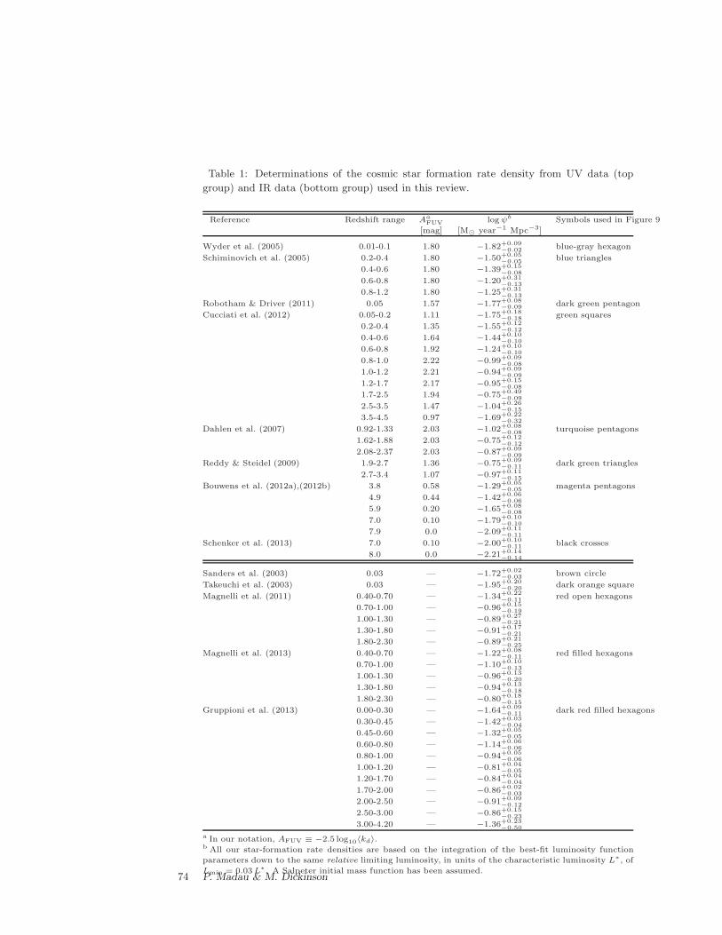
Table 1: Determinations of the cosmic star formation rate density from UV data (top

group) and IR data (bottom group) used in this review.

Reference Redshift range Aa

FUV logψb Symbols used in Figure 9

[mag] [M⊙ year−1 Mpc−3]

Wyder et al. (2005) 0.01-0.1 1.80 −1.82+0.09

−0.02blue-gray hexagon

Schiminovich et al. (2005) 0.2-0.4 1.80 −1.50+0.05

−0.05blue triangles

0.4-0.6 1.80 −1.39+0.15

−0.08

0.6-0.8 1.80 −1.20+0.31

−0.13

0.8-1.2 1.80 −1.25+0.31

−0.13

Robotham & Driver (2011) 0.05 1.57 −1.77+0.08

−0.09dark green pentagon

Cucciati et al. (2012) 0.05-0.2 1.11 −1.75+0.18

−0.18green squares

0.2-0.4 1.35 −1.55+0.12

−0.12

0.4-0.6 1.64 −1.44+0.10

−0.10

0.6-0.8 1.92 −1.24+0.10

−0.10

0.8-1.0 2.22 −0.99+0.09

−0.08

1.0-1.2 2.21 −0.94+0.09

−0.09

1.2-1.7 2.17 −0.95+0.15

−0.08

1.7-2.5 1.94 −0.75+0.49

−0.09

2.5-3.5 1.47 −1.04+0.26

−0.15

3.5-4.5 0.97 −1.69+0.22

−0.32

Dahlen et al. (2007) 0.92-1.33 2.03 −1.02+0.08

−0.08turquoise pentagons

1.62-1.88 2.03 −0.75+0.12

−0.12

2.08-2.37 2.03 −0.87+0.09

−0.09

Reddy & Steidel (2009) 1.9-2.7 1.36 −0.75+0.09

−0.11dark green triangles

2.7-3.4 1.07 −0.97+0.11

−0.15

Bouwens et al. (2012a),(2012b) 3.8 0.58 −1.29+0.05

−0.05magenta pentagons

4.9 0.44 −1.42+0.06

−0.06

5.9 0.20 −1.65+0.08

−0.08

7.0 0.10 −1.79+0.10

−0.10

7.9 0.0 −2.09+0.11

−0.11

Schenker et al. (2013) 7.0 0.10 −2.00+0.10

−0.11black crosses

8.0 0.0 −2.21+0.14

−0.14

Sanders et al. (2003) 0.03 — −1.72+0.02

−0.03brown circle

Takeuchi et al. (2003) 0.03 — −1.95+0.20

−0.20dark orange square

Magnelli et al. (2011) 0.40-0.70 — −1.34+0.22

−0.11red open hexagons

0.70-1.00 — −0.96+0.15

−0.19

1.00-1.30 — −0.89+0.27

−0.21

1.30-1.80 — −0.91+0.17

−0.21

1.80-2.30 — −0.89+0.21

−0.25

Magnelli et al. (2013) 0.40-0.70 — −1.22+0.08

−0.11red filled hexagons

0.70-1.00 — −1.10+0.10

−0.13

1.00-1.30 — −0.96+0.13

−0.20

1.30-1.80 — −0.94+0.13

−0.18

1.80-2.30 — −0.80+0.18

−0.15

Gruppioni et al. (2013) 0.00-0.30 — −1.64+0.09

−0.11dark red filled hexagons

0.30-0.45 — −1.42+0.03

−0.04

0.45-0.60 — −1.32+0.05

−0.05

0.60-0.80 — −1.14+0.06

−0.06

0.80-1.00 — −0.94+0.05

−0.06

1.00-1.20 — −0.81+0.04

−0.05

1.20-1.70 — −0.84+0.04

−0.04

1.70-2.00 — −0.86+0.02

−0.03

2.00-2.50 — −0.91+0.09

−0.12

2.50-3.00 — −0.86+0.15

−0.23

3.00-4.20 — −1.36+0.23

−0.50

a In our notation, AFUV ≡ −2.5 log10〈kd〉.b All our star-formation rate densities are based on the integration of the best-fit luminosity function

parameters down to the same relative limiting luminosity, in units of the characteristic luminosity L∗, of

Lmin = 0.03L∗. A Salpeter initial mass function has been assumed.74 P. Madau & M. Dickinson

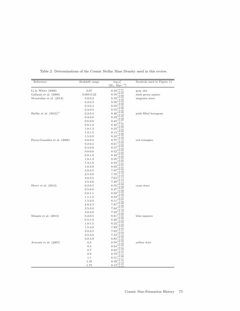
Table 2: Determinations of the Cosmic Stellar Mass Density used in this review.

Reference Redshift range log ρa∗ Symbols used in Figure 11

[M⊙ Mpc−3]

Li & White (2009) 0.07 8.59+0.01

−0.01gray dot

Gallazzi et al. (2008) 0.005-0.22 8.78+0.07

−0.08dark green square

Moustakas et al. (2013) 0.0-0.2 8.59+0.05

−0.05magenta stars

0.2-0.3 8.56+0.09

−0.09

0.3-0.4 8.59+0.06

−0.06

0.4-0.5 8.55+0.08

−0.08

Bielby et al. (2012) b 0.2-0.4 8.46+0.09

−0.12pink filled hexagons

0.4-0.6 8.33+0.03

−0.03

0.6-0.8 8.45+0.08

−0.1

0.8-1.0 8.42+0.05

−0.06

1.0-1.2 8.25+0.04

−0.04

1.2-1.5 8.14+0.06

−0.06

1.5-2.0 8.16+0.32

−0.03

Perez-Gonzalez et al. (2008) 0.0-0.2 8.75+0.12

−0.12red triangles

0.2-0.4 8.61+0.06

−0.06

0.4-0.6 8.57+0.04

−0.04

0.6-0.8 8.52+0.05

−0.05

0.8-1.0 8.44+0.05

−0.05

1.0-1.3 8.35+0.05

−0.05

1.3-1.6 8.18+0.07

−0.07

1.6-2.0 8.02+0.07

−0.07

2.0-2.5 7.87+0.09

−0.09

2.5-3.0 7.76+0.18

−0.18

3.0-3.5 7.63+0.14

−0.14

3.5-4.0 7.49+0.13

−0.13

Ilbert et al. (2013) 0.2-0.5 8.55+0.08

−0.09cyan stars

0.5-0.8 8.47+0.07

−0.08

0.8-1.1 8.50+0.08

−0.08

1.1-1.5 8.34+0.10

−0.07

1.5-2.0 8.11+0.05

−0.06

2.0-2.5 7.87+0.08

−0.08

2.5-3.0 7.64+0.15

−0.14

3.0-4.0 7.24+0.18

−0.20

Muzzin et al. (2013) 0.2-0.5 8.61+0.06

−0.06blue squares

0.5-1.0 8.46+0.03

−0.03

1.0-1.5 8.22+0.03

−0.03

1.5-2.0 7.99+0.05

−0.03

2.0-2.5 7.63+0.11

−0.04

2.5-3.0 7.52+0.13

−0.09

3.0-4.0 6.84+0.43

−0.20

Arnouts et al. (2007) 0.3 8.78+0.12

−0.16yellow dots

0.5 8.64+0.09

−0.11

0.7 8.62+0.08

−0.10

0.9 8.70+0.11

−0.15

1.1 8.51+0.08

−0.11

1.35 8.39+0.10

−0.13

1.75 8.13+0.10

−0.13


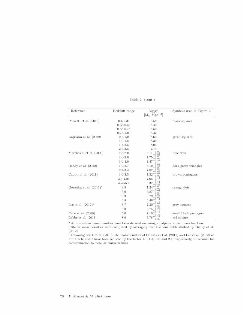
Table 2: (cont.)

Reference Redshift range log ρa∗ Symbols used in Figure 11[M⊙ Mpc−3]

Pozzetti et al. (2010) 0.1-0.35 8.58 black squares0.35-0.55 8.490.55-0.75 8.500.75-1.00 8.42

Kajisawa et al. (2009) 0.5-1.0 8.63 green squares1.0-1.5 8.301.5-2.5 8.042.5-3.5 7.74

Marchesini et al. (2009) 1.3-2.0 8.11+0.02−0.02 blue dots

2.0-3.0 7.75+0.05−0.04

3.0-4.0 7.47+0.37−0.13

Reddy et al. (2012) 1.9-2.7 8.10+0.03−0.03 dark green triangles

2.7-3.4 7.87+0.03−0.03

Caputi et al. (2011) 3.0-3.5 7.32+0.04−0.02 brown pentagons

3.5-4.25 7.05+0.11−0.10

4.25-5.0 6.37+0.14−0.54

Gonzalez et al. (2011)c 3.8 7.24+0.06−0.06 orange dots

5.0 6.87+0.08−0.09

5.9 6.79+0.09−0.09

6.8 6.46+0.14−0.17

Lee et al. (2012)c 3.7 7.30+0.07−0.09 gray squares

5.0 6.75+0.33−0.16

Yabe et al. (2009) 5.0 7.19+0.19−0.35 small black pentagon

Labbe et al. (2013) 8.0 5.78+0.22−0.30 red square

a All the stellar mass densities have been derived assuming a Salpeter initial mass function.b Stellar mass densities were computed by averaging over the four fields studied by Bielby et al.(2012).c Following Stark et al. (2013), the mass densities of Gonzalez et al. (2011) and Lee et al. (2012) atz ≃ 4, 5, 6, and 7 have been reduced by the factor 1.1, 1.3, 1.6, and 2.4, respectively, to account forcontamination by nebular emission lines.


Documents

Cosmic Star-FormationHistory arXiv:1403.0007v3 [astro-ph