MNRAS 000, 000–000 (0000) Preprint 16 November 2021 Compiled using MNRAS LATEX style file v3.0

Cosmic Shear in Harmonic Space from the Dark EnergySurvey Year 1 Data: Compatibility with ConfigurationSpace Results

H. Camacho,1,2 F. Andrade-Oliveira,1,2 A. Troja,3,2 R. Rosenfeld,3,2 L. Faga,4,2 R. Gomes,4,2

C. Doux,5 X. Fang,6,7 M. Lima,4,2 V. Miranda,7 T. F. Eifler,7,8 O. Friedrich,9 M. Gatti,5

G. M. Bernstein,5 J. Blazek,10,11 S. L. Bridle,12 A. Choi,13 C. Davis,14 J. DeRose,15

E. Gaztanaga,16,17 D. Gruen,18 W. G. Hartley,19 B. Hoyle,18 M. Jarvis,5 N. MacCrann,20

J. Prat,21,22 M. M. Rau,23 S. Samuroff,23 C. Sanchez,5 E. Sheldon,24 M. A. Troxel,25 P. Vielzeuf,26

J. Zuntz,27 T. M. C. Abbott,28 M. Aguena,2 S. Allam,29 J. Annis,29 D. Bacon,30 E. Bertin,31,32

D. Brooks,33 D. L. Burke,14,34 A. Carnero Rosell,2 M. Carrasco Kind,35,36 J. Carretero,26

F. J. Castander,16,17 R. Cawthon,37 M. Costanzi,38,39,40 L. N. da Costa,2,41 M. E. S. Pereira,42,43

J. De Vicente,44 S. Desai,45 H. T. Diehl,29 P. Doel,33 S. Everett,46 A. E. Evrard,47,42

I. Ferrero,48 B. Flaugher,29 P. Fosalba,16,17 D. Friedel,35 J. Frieman,29,22 J. Garcıa-Bellido,49

D. W. Gerdes,47,42 R. A. Gruendl,35,36 J. Gschwend,2,41 G. Gutierrez,29 S. R. Hinton,50

D. L. Hollowood,46 K. Honscheid,51,52 D. Huterer,42 D. J. James,53 K. Kuehn,54,55 N. Kuropatkin,29

O. Lahav,33 M. A. G. Maia,2,41 J. L. Marshall,56 P. Melchior,57 F. Menanteau,35,36 R. Miquel,58,26

R. Morgan,59 F. Paz-Chinchon,35,60 D. Petravick,35 A. Pieres,2,41 A. A. Plazas Malagon,57 K. Reil,34

M. Rodriguez-Monroy,44 E. Sanchez,44 V. Scarpine,29 M. Schubnell,42 S. Serrano,16,17 I. Sevilla-Noarbe,44 M. Smith,61 M. Soares-Santos,42 E. Suchyta,62 G. Tarle,42 D. Thomas,30 C. To,63,14,34

T. N. Varga,64,65 J. Weller,64,65 and R.D. Wilkinson66

(DES Collaboration)

16 November 2021

ABSTRACTWe perform a cosmic shear analysis in harmonic space using the first year of datacollected by the Dark Energy Survey (DES-Y1). We measure the cosmic weak lensingshear power spectra using the metacalibration catalogue and perform a likelihoodanalysis within the framework of CosmoSIS. We set scale cuts based on baryonic ef-fects contamination and model redshift and shear calibration uncertainties as well asintrinsic alignments. We adopt as fiducial covariance matrix an analytical computa-tion accounting for the mask geometry in the Gaussian term, including non-Gaussiancontributions. A suite of 1200 lognormal simulations is used to validate the harmonicspace pipeline and the covariance matrix. We perform a series of stress tests to gaugethe robustness of the harmonic space analysis. Finally, we use the DES-Y1 pipelinein configuration space to perform a similar likelihood analysis and compare both re-sults, demonstrating their compatibility in estimating the cosmological parameters S8,σ8 and Ωm. The methods implemented and validated in this paper will allow us toperform a consistent harmonic space analysis in the upcoming DES data.

Key words: cosmology: observations (cosmology:) large-scale structure of Universe

1 INTRODUCTION

One of the consequences of the Theory of General Relativityis the precise prediction of the deflection of light due to the

presence of matter in its path (Einstein 1916). This predic-tion was confirmed for the first time with the measurementsof the positions of stars during a solar eclipse in 1919 by twoexpeditions, sent to Brazil and to the Principe Island (Dyson

© 0000 The Authors

arX

iv:2

111.

0720

3v1

[as

tro-

ph.C

O]

13

Nov

202

1

2 DES Collaboration

et al. 1920). After roughly 100 years, and the enormous de-velopment of instrumental and theoretical methods, one isable to measure minute distortions in the shape of distantgalaxies that provide information about the distribution ofmatter in the universe. These small distortions are calledweak gravitational lensing, in opposition to strong gravita-tional lensing, when large distortions with multiple images ofthe same object are produced (for reviews see, e.g. Bartel-mann & Schneider (2001); Dodelson (2017); Mandelbaum(2018)).

Being a small effect, weak gravitational lensing can bedetected only by capturing the images of a large sampleof galaxies, usually called source galaxies, and performingshape measurements that can then be analyzed statisti-cally. One of the most common ways to analyse weak lens-ing signals is by studying the correlation between shapesof two galaxies. This can be done in configuration space,with measurements of the two-point correlation functions,or in harmonic space and the corresponding measurementof the power spectra. Although they are both second orderstatistics and can be related by a Fourier transform, theyprobe scales differently, and so they behave differently tosystematic effects and analysis choices. In practice, thereare differences in the measurements and analyses that mayyield different cosmological results from the configurationand harmonic space methods (Hamana et al. 2020). In par-ticular, the covariance matrix is known to be more diagonal(indicating less cross-correlations) in harmonic space thanin configuration space due to the orthogonality of the spher-ical harmonics used to decompose the signal (see e.g., figure2 in DES Collaboration et al. (2021)). The consistency be-tween cosmic shear analyses in configuration and harmonicspace was recently investigated in Doux et al. (2021b), usingDES-Y3-like Gaussian mock catalogues and paying partic-ular attention to the methodology of determining angularand multipole scale cuts in both cases.

In the past years, several collaborations reported re-sults from weak gravitational lensing: the Deep Lens Survey(DLS)1, the Canada-France-Hawaii Telescope Lensing Sur-vey (CFHTLenS)2, the Hyper Suprime-Cam Subaru Strate-gic Program (HSC-SSP)3, the Kilo-Degree Survey (KiDS)4

and the Dark Energy Survey (DES)5. DLS (Jee et al. 2013,2016) and CFHTLenS (Joudaki et al. 2017) presented re-sults from configuration space measurements whereas HSChas performed the analysis both in harmonic space (Hikageet al. 2019) and configuration space (Hamana et al. 2020).KiDS has performed a cosmic shear analysis in configura-tion space for its 450 deg2 survey (Hildebrandt et al. 2017)and for its fourth data release (KiDS-1000) a comparisonof configuration and harmonic space analyses was presentedand showed excellent agreement (Asgari et al. 2021). For itsfirst year of data (Y1), DES has presented a weak lensinganalysis in configuration space only (Troxel et al. 2018).

Two re-analyses of DES-Y1 weak gravitational lens-ing in combination with other experiments have been per-formed: KiDS-450 and DES-Y1 (Joudaki et al. 2020), and

1 dls.physics.ucdavis.edu2 www.cfhtlens.org3 hsc.mtk.nao.ac.jp/ssp4 kids.strw.leidenuniv.nl5 www.darkenergysurvey.org

DLS, CFHTLens, KiDS-450 and the DES Science Verifica-tion data (Chang et al. 2019). More recently, the DES-Y1public data was used to perform a full 3x2pt analysis (thecombination of shear, galaxy clustering and galaxy-galaxylensing) in harmonic space with emphasis on the testing of amore sophisticated model for galaxy bias (Hadzhiyska et al.2021).

The purpose of this paper is to complete the Y1 weaklensing analysis by presenting harmonic space results andcomparing them to the configuration space ones. We mea-sure the cosmic weak lensing shear power spectra using theso-called metacalibration catalogs. We perform a likeli-hood analysis using the framework of CosmoSIS adopted byDES assuming a fiducial ΛCDM cosmological model withparameters given in the Table 1. We use 1200 lognormalsimulations developed for DES-Y1 to validate an analyticalcovariance matrix and scale cuts tested to curb the contri-butions from baryonic effects to the shear power spectra.We also use the DES-Y1 pipeline in configuration space toperform a similar likelihood analysis and compare both re-sults, demonstrating their compatibility. The methods im-plemented and verified in this paper will allow us to performan independent harmonic space analysis for the upcomingDES data.

This paper is organized as follows. Section 2 reviewsthe basic theoretical modelling, including systematic effectssuch as redshift uncertainties, shear calibration and intrin-sic alignments. In Section 3 we describe the DES-Y1 datafor the shear analysis presented here, Section 4 presents the1200 flask lognormal mocks used to validate our pipelineand the analytical covariance matrix. Section 5 details ourmethodology including a discussion of the covariance matrix.We perform likelihood analyses both in harmonic and con-figuration space and present our main results in Section 6,with some robustness tests shown in Section 7. We concludein Section 8.

2 THEORETICAL MODELLING

The distortion of the shape of an object due to the inter-vening matter is described by a lens potential ϕ(~θ) that isrelated to the projection of the gravitational potential Φ(~r)along the line-of-sight from the source (S) to us (we will de-note the comoving distance by χ and use units where c = 1):

ϕ(~θ) =2

χS

∫ χS

0

dχχS − χχ

Φ(χ, ~θ). (1)

The convergence (κ) and shear (γ1 and γ2) fields arederived from the lens potential as 6:

κ(~θ) =1

2

(∂2ϕ

∂θ21

+∂2ϕ

∂θ22

), (2)

γ1(~θ) =1

2

(∂2ϕ

∂θ21

− ∂2ϕ

∂θ22

), (3)

γ2(~θ) =∂2ϕ

∂θ1∂θ2. (4)

6 Following Troxel et al. (2018), throughout this work we assume

the flat-sky approximation.

MNRAS 000, 000–000 (0000)

DES-Y1 Cosmic Shear in Harmonic Space 3

Using the Poisson equation one can write the conver-gence in terms of the density perturbation δ = δρ/ρ as:

κ(~θ) =

∫ χS

0

dχWκ(~θ)δ(χ, ~θ), (5)

where the lensing window function Wκ(χ) can be definedby:

Wκ(χ) =3H2

0 Ωmχ

2a(χ)

∫ χH

χ

dχSdn

dz(z(χS))

dz

dχS

(1− χ

χS

),

(6)where χH is the comoving distance to the cosmic horizonand for multiple galaxy sources described by a redshift dis-tribution normalised as:∫ ∞

0

dzdn

dz(z) = 1. (7)

In harmonic space we can write the convergence andshear fields as:

κ(~) = −|`|2

2ϕ(~), (8)

γ1(~) =`22 − `21

2ϕ(~), (9)

γ2(~) = −`1`2ϕ(~). (10)

The convergence and shear fields are not independentsince they are determined by the gravitational potential.One can find linear combinations of γ1 and γ2, the so-calledE and B modes denoted by γE and γB such that:

γE(~) = κ(~); γB(~) = 0. (11)

Finally, we are interested in the 2-point correlations be-tween these fields. In the Limber approximation (Limber1953; LoVerde & Afshordi 2008; Kitching et al. 2017) theE-mode angular power spectrum CEE(`) (which is equal tothe convergence angular power spectrum Cκκ(`)) is givenby:

CEE(i,j)(`) =

∫ χH

0

dχW iκ(χ)W j

κ(χ)

χ2Pm

(`+ 1/2

χ, χ

), (12)

where we have introduced indices for the different tomo-graphic redshift bins (i, j) that will be used in the analy-ses and Pm is the total matter power spectrum, modelledhere to include nonlinear effects using the CAMB Boltz-mann solver (Lewis et al. 2000; Howlett et al. 2012) and theHALOFIT (Smith et al. 2003) prescription with updatesfrom Takahashi et al. (2012). The shear angular correla-tion functions ξ±(θ) that are also used in the comparisonperformed in this paper can be computed from the angu-lar power spectra (see, e.g. equation (9) in Friedrich et al.(2021)).

We also model three astrophysical and observationalsystematic effects using the DES-Y1 methodology (see de-tails in Krause et al. (2017); Troxel et al. (2018)):

• Redshift distributions: an additive bias ∆zi on themean of the redshift distribution of source galaxies in eachtomographic bin i is introduced to account for uncertaintieson the photometric redshift estimation;• Shear calibration: a multiplicative bias on the shear am-

plitude is included in each tomographic bin i to account foruncertainties on the shear calibration and included in ourpower spectra modelling as (Heymans et al. 2006; Hutereret al. 2006) CEE(i,j)(`) = (1 +mi)(1 +mj)CEE,true

(i,j) (`);

• Intrinsic alignments: we use the nonlinear alignmentmodel (NLA) (Kirk et al. 2012; Bridle & King 2007)for the intrinsic alignment corrections to the cosmic-shear power spectrum, where the redshift evolution ofthe nonlinear alignment amplitude is parameterised asAIA [(1 + z)/(1 + z0)]αIA , with z0 = 0.62 fixed at the meanredshift of source galaxies and AIA, αIA are free parametersin our model7.

All the different pieces for the modelling presentedabove are used as modules in the, publicly available, Cos-moSIS framework (Zuntz et al. 2015), in an analogous wayto what was done for the configuration-space analysis pre-sented in Troxel et al. (2018). Finally, the theoretical angularpower spectrum is binned in bandpowers using the prescrip-tion given in Alonso et al. (2019). The data, priors and red-shift distributions are introduced in the following section.

3 DATA

The Dark Energy Survey (DES) conducted its six-year sur-vey finalising in January 2019 using a 570-megapixel cam-era mounted on the 4-meter Blanco Telescope at the CerroTololo Inter-American Observatory (CTIO). The photomet-ric survey used five filters and collected information of morethan 300 million galaxies in an area of roughly 5000 deg2,allowing for the measurement of shapes in addition to posi-tions of galaxies.

The analysis of the first year of data, denoted by DES-Y1, used two independent pipelines (Zuntz et al. 2018) toproduce shape catalogues for its shear analysis: metacal-ibration and im3shape. Here we will focus on the meta-calibration catalogue that was used in the real-space fidu-cial analysis, with a final contiguous area of 1321 deg2 con-taining 26 million galaxies with a density of 5.5 galaxiesarcmin−2. A Bayesian Photometric Redshift (BPZ) (Benıtez2000) method was used to divide these source objects intofour tomographic redshift bins shown in Table 2. The priorson the redshift (Hoyle et al. 2018; Davis et al. 2017; Gattiet al. 2018) and shear calibration (Zuntz et al. 2018) param-eters are shown in the Table 1.

In order to correct noise, modelling, and selection bi-ases in the shear estimate, one uses the metacalibrationmethod (Huff & Mandelbaum 2017; Sheldon & Huff 2017).It introduces a shear response correction (a 2× 2 matrix Rifor each object i) that is obtained by artificially shearingeach image in the catalogue and has two components: a re-sponse of the shape estimator and a response of the selectionof the objects. metacalibration does not use a per-galaxyweight and the shear response corrections are made avail-able in the catalogue release8. The shear response is usedto obtain the estimated calibrated shear ~γi for each objectfrom the measured ellipticities as (Zuntz et al. 2018):

~γi = 〈Ri〉−1~ei, (13)

7 In the DES-Y1 analysis a more sophisticated ‘tidal alignmentand tidal torquing’ (TATT) model (Blazek et al. 2019) for intrin-

sic alignment was also considered and found to be not required forthe Y1 configuration. It became the fiducial choice in DES-Y3.8 The DES Y3 analysis now implement those weights (Gatti

2021).

MNRAS 000, 000–000 (0000)

4 DES Collaboration

where we use an averaged response matrix for each tomo-graphic redshift bin and have also subtracted a nonzeromean 〈~ei〉 per tomographic bin prior to the shear estimation.The estimated shear per object is pixelated in maps usingthe HEALPix pixelisation scheme (Gorski et al. 2005) witha resolution Nside = 1024 for each redshift bin9 and theangular power spectrum is measured using NaMASTER(Alonso et al. 2019) as described in Section 5.

4 LOGNORMAL MOCK CATALOGUES

We use a set of 1200 lognormal realisations generatedwith the Full-sky Lognormal Astro-fields Simulation Kit(flask10) (Xavier et al. 2016), specially designed for DESY1 configuration-space analysis (Krause et al. 2017; Troxelet al. 2018) in order to test our pipeline and validate thefiducial covariance presented in this analysis.

The lognormal flask realisations use as input the an-gular power spectrum for each pair of redshift bins (i, j).Those were computed using CosmoLike (Krause & Eifler2017) from a ΛCDM cosmological model with parametersquoted as fiducial in Table 1 and redshift distributions forfour tomographic redshift bins that were used in the paperdescribing the DES-Y1 methodology (Krause et al. 2017)and the paper reporting DES-Y1 cosmological results fromcosmic shear (Troxel et al. 2018).

On top of the one- and two-point distributions, thissuite of realisations were also designed to match the reducedskewness of projected fields predicted by perturbation the-ory at a fiducial scale of 10 Mpch−1, see Friedrich et al.(2018); Krause et al. (2017) for details. This approach hasbeen shown to yield accurate results for DES-Y1 (Krauseet al. 2017) and DES-Y3 (Friedrich et al. 2021) two-pointobservables. We also note that Friedrich et al. (2021) hadshown, also in the context of DES analysis, that the non-connected part of the covariance matrix does not cause sig-nificant bias in a cosmological analysis.

The flask shear maps are generated using HEALPixwith resolution set by an Nside parameter of 4096. We fur-ther sample source galaxy positions and ellipticity dispersionfor each tomographic bin by matching the observed numberdensity of galaxies neff and the shape-noise parameter σe.The numbers used for the flask mocks are given in Table 2and are similar to the values used in Troxel et al. (2018).

5 METHODS

In this section, we present the methodology to be used in ouranalysis. We begin by describing the angular power spectraestimation, followed by a discussion of the scale-cuts chosento mitigate baryonic effects and end with a discussion of thefiducial covariance matrix used in this work.

9 All DES Y1/Y3 map-based analyses are performed at this reso-lution because it is a good trade-off between resolution and num-

ber of galaxies per pixel (see e.g. Chang et al. (2018)).10 www.astro.iag.usp.br/∼flask

Parameter Fiducial value Prior

Ωm 0.286 U(0.1, 0.9)

h 0.70 U(0.55, 0.90)

Ωb 0.05 U(0.03, 0.07)ns 0.96 U(0.87, 1.07)

As × 109 2.232746 U(0.5, 5.0)

Ωνh2 0.0 U(0.0, 0.01)

AIA 0 U(−5.0, 5.0)

αIA 0 U(−5.0, 5.0)

(m1 – m4)×102 0 N(1.2, 2.3)

∆z1 × 102 0 N(−0.1, 1.6)∆z2 × 102 0 N(−1.9, 1.3)

∆z3 × 102 0 N(0.9, 1.1)∆z4 × 102 0 N(−1.8, 2.2)

Table 1. The cosmological and nuisance parameters used in Y1

analysis. The fiducial values were used in the generation of the1200 flask mocks for DES-Y1. The priors were used for DES-Y1

real-space likelihood analysis.

redshift bin neff σe

0.20 < zphot < 0.43 1.5 0.3

0.43 < zphot < 0.63 1.5 0.30.63 < zphot < 0.90 1.5 0.3

0.90 < zphot < 1.30 1.7 0.3

Table 2. Effective angular number density and shear dispersionfor each tomographic redshift bin.

5.1 Angular power spectrum measurements

For the angular power spectra estimation, we use the so-called pseudo-C` or MASTER method (Hivon et al. 2002),as implemented in the NaMASTER code 11 (Alonso et al.2019).

For the pixelized representation of cosmic shear cata-logs, we construct weighted tomographic cosmic shear maps,

~γp =∑i∈p

vi~γi/∑i∈p

vi, (14)

where p runs over pixels and i ∈ p runs over the galaxiesin each pixel, ~γi = (γ1, γ2) is the calibrated galaxy shear(see eq. (13)) and vi its associated weight. Throughout thiswork we use a HEALPix fiducial resolution Nside = 1024,which corresponds to a typical pixel size of the order of 3.4arcminutes.

In addition to the cosmic shear signal maps, the pseudo-C` method relies on the use of an angular window function,also known as the mask. Such a mask encodes the informa-tion of the partial-sky coverage of the observed signal andis used to deconvolve this effect on the estimated bandpow-ers. In this work, we use the sum of weights scheme pre-sented in Nicola et al. (2021), and construct tomographic

11 github.com/LSSTDESC/NaMaster

MNRAS 000, 000–000 (0000)

DES-Y1 Cosmic Shear in Harmonic Space 5

mask maps as

wp =∑i∈p

vi , (15)

where the vi are the individual galaxy weights assigned bymetacalibration. It is important to notice that in thisapproach there are different masks constructed for each to-mographic bin, since the number of galaxies per pixel variesfor each bin. In practical terms, these masks are equivalentto the pixelised weighted galaxy-count maps.

An important part of power spectra estimation is theso-called noise bias, always present on the raw signal auto-correlation measurements because of the discrete nature ofthe signal maps inherited from the galaxy catalogues. Forthe specific case of the pseudo-C` algorithm, it must be sub-tracted from the auto-correlations in order to obtain an un-biased estimate of the signal power spectrum. Schematically,the true binned power spectrum estimator can be written as(Alonso et al. 2019):

Cabq =∑q′

(Mab)−1qq′

(Cabq′ − δabNb

q′

), (16)

where Mabqq′ =

∑`∈q,`′∈q′ w

`qM

ab``′ is the binned version of

the coupling matrix, Mab``′ , that can be calculated analyti-

cally and depends on the mask maps for the tomographicbins a and b, Cabq =

∑`∈q w

`qw

`qC

ab` is the binned version of

the pseudo-C`, Cab` . Here q, q′ represent multipole bins or

bandpowers and w`q are multipole weights defined for ` ∈ qand normalized to

∑`∈q w

`q = 1 12, see (Alonso et al. 2019)

for more details. Finally, Nq =∑`∈q w

`qN` are the binned

version of the noise bias pseudo-spectra, N`, given (in thesum of weights scheme) by (Nicola et al. 2021):

N` = Apix

⟨∑i∈p

v2i σ

2γ,i

⟩pix

, (17)

where the average 〈·〉pix is over all the pixels, Apix is the areaof the pixels on the chosen HEALPix resolution and

σ2γ,i =

1

2

(γ2

1,i + γ22,i

)(18)

is the estimated shear variance of each galaxy. Notice thatthe noise-bias pseudo-power spectrum N` is independent ofthe ` multipole. The true noise-bias power spectrum N` isobtained using the NaMASTER method, deconvolving themask and performing the same ` binning as the signal. Thisnoise bias contribution, subtracted from the measurements,must be included in the covariance matrix, as we will discussbelow.

5.2 Binning and scale-cuts

For all the angular power spectra measured here, we con-sider angular multipoles ` ∈ [30, 3000) divided into 20logarithmic-spaced bandpowers with edges similar to thebinning scheme used in Andrade-Oliveira et al. (2021),where analysis of DES-Y1 galaxy clustering in harmonicspace is performed.

12 Troughout this work we assume equal weights for all multi-

poles on each bandpower.

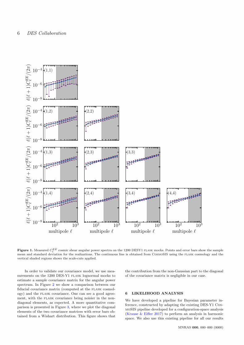
A comparison between the measured cosmic shear an-gular power spectra on the mocks and the input theory pre-diction used for its generation is shown in Figure 1. We findvery good agreement, validating the measurement pipeline(namely, the noise-subtraction method and the computationof the coupling matrix).

Scale cuts are a key factor for cosmic shear analyses(see, e.g. Doux et al. (2021b)). For the small scales, we fol-low the DES-Y1 configuration-space analysis and cut-outscales where baryonic effects introduce a significant bias inthe angular power spectra (Troxel et al. 2018). To estimatethe impact of baryon physics, the OWLS (OverWhelminglyLarge Simulations project) suite of hydrodynamic simula-tions (van Daalen et al. 2011; Schaye et al. 2010) is used forre-scaling the computed non-linear power spectrum in ourfiducial model prediction by a factor

PNL(k)→ PDM+Baryon(k)

PDM(k)× PNL(k), (19)

where ‘DM’ refers to the power spectrum from the OWLSdark-matter-only simulation, while ‘DM+Baryon’ refers tothe power spectrum from the OWLS AGN simulation (vanDaalen et al. 2011; Schaye et al. 2010). It is importantto note that the particular use of the OWLS simulations,among others for DES-Y1 analysis, is a conservative choice,as they offer some of the most significant deviations from theDM cases in the power spectrum Troxel et al. (2018). Wethen compare the predictions for the cosmic-shear angularpower spectra with and without the re-scaling for PNL(k)and impose, for our fiducial analysis, the same 2% thresholdimposed by the configuration space analysis (Troxel et al.2018). Hence we remove from our data vector all bandpowerswith a fractional contribution from baryonic effects greaterthan 2% in our fiducial model for each pair of redshift bins.

We adopt a fiducial value for the lower multipole value` > 30 and test a different value as a robustness test. Ourfinal data vector ends up having a total of 85 entries. Wenote that an improvement should be expected by includingbaryonic effects in the modelling and relaxing the proposedscale cuts. As already shown in configuration space (Huanget al. 2021; Moreira et al. 2021) such improvement can beof ∼ 20% on the recovered constraints.

5.3 Covariance matrix

The covariance matrix has Gaussian, non-Gaussian andnoise contributions and we use two different methods tocompute them. For the Gaussian contribution, we rely on theso-called improved narrow-kernel approximation (iNKA) ap-proach within the pseudo-C` framework that takes into ac-count the geometry of the finite survey area described by themask maps (Garcıa-Garcıa et al. 2019; Nicola et al. 2021).We also use the full model for the noise terms in the pseudo-spectra Gaussian covariance as given by Nicola et al. (2021)(their equation (2.29)). The non-Gaussian contribution con-sists of the so-called super-sample covariance (SSC) and theconnected part of the 4-point function. These are obtainedusing the halo model analytical computations with the Cos-moLike code (Krause & Eifler 2017) in harmonic space13.

13 DES-Y1 and Y3 analyses in configuration space use Cosmo-

Like covariance matrices as fiducial.

MNRAS 000, 000–000 (0000)

6 DES Collaboration

10−8

10−6

10−4

`(`

+1)C

EE

`/(

2π)

(1,1)

10−8

10−6

10−4

`(`

+1)C

EE

`/(

2π)

(1,2) (2,2)

10−8

10−6

10−4

`(`

+1)C

EE

`/(

2π)

(1,3) (2,3) (3,3)

102 103

multipole `

10−8

10−6

10−4

`(`

+1)C

EE

`/(

2π)

(1,4)

102 103

multipole `

(2,4)

102 103

multipole `

(3,4)

102 103

multipole `

(4,4)

Figure 1. Measured CEE` cosmic shear angular power spectra on the 1200 DESY1 flask mocks. Points and error bars show the sample

mean and standard deviation for the realizations. The continuous line is obtained from CosmoSIS using the flask cosmology and the

vertical shaded regions shows the scale-cuts applied.

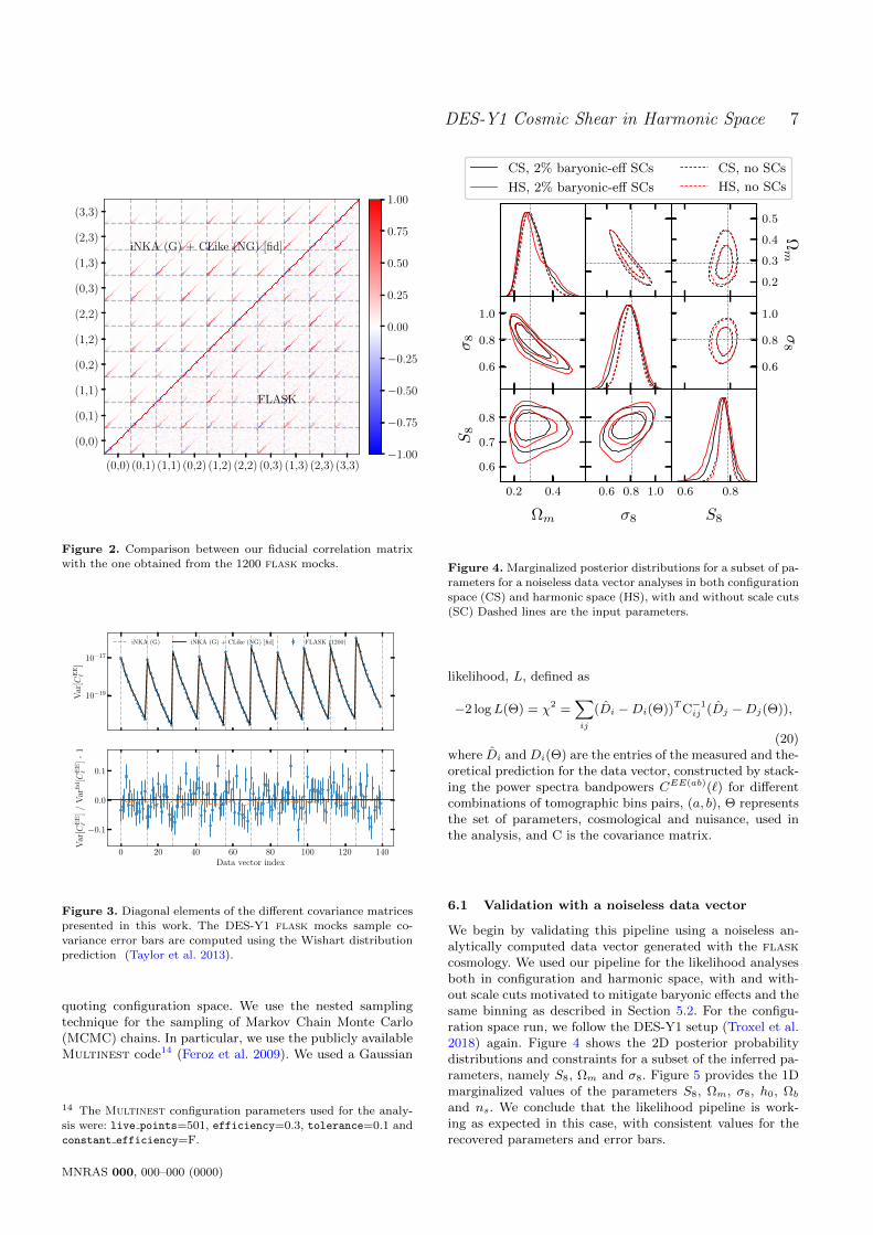
In order to validate our covariance model, we use mea-surements on the 1200 DES-Y1 flask lognormal mocks toestimate a sample covariance matrix for the angular powerspectrum. In Figure 2 we show a comparison between ourfiducial covariance matrix (computed at the flask cosmol-ogy) and the flask covariance. One can see a good agree-ment, with the flask covariance being noisier in the non-diagonal elements, as expected. A more quantitative com-parison is presented in Figure 3, where we plot the diagonalelements of the two covariance matrices with error bars ob-tained from a Wishart distribution. This figure shows that

the contribution from the non-Gaussian part to the diagonalof the covariance matrix is negligible in our case.

6 LIKELIHOOD ANALYSIS

We have developed a pipeline for Bayesian parameter in-ference, constructed by adapting the existing DES-Y1 Cos-moSIS pipeline developed for a configuration-space analysis(Krause & Eifler 2017) to perform an analysis in harmonicspace. We also use this existing pipeline for all our results

MNRAS 000, 000–000 (0000)

DES-Y1 Cosmic Shear in Harmonic Space 7

(0,0) (0,1) (1,1) (0,2) (1,2) (2,2) (0,3) (1,3) (2,3) (3,3)

(0,0)

(0,1)

(1,1)

(0,2)

(1,2)

(2,2)

(0,3)

(1,3)

(2,3)

(3,3)

iNKA (G) + CLike (NG) [fid]

FLASK

−1.00

−0.75

−0.50

−0.25

0.00

0.25

0.50

0.75

1.00

Figure 2. Comparison between our fiducial correlation matrix

with the one obtained from the 1200 flask mocks.

10−19

10−17

Var

[CE

E`

]

iNKA (G) iNKA (G) + CLike (NG) [fid] FLASK (1200)

0 20 40 60 80 100 120 140Data vector index

−0.1

0.0

0.1

Var

[CE

E`

]/

Var

fid[C

EE

`]

-1

(0,0) (0,1) (1,1) (0,2) (1,2) (2,2) (0,3) (1,3) (2,3) (3,3)

Figure 3. Diagonal elements of the different covariance matrices

presented in this work. The DES-Y1 flask mocks sample co-variance error bars are computed using the Wishart distribution

prediction (Taylor et al. 2013).

quoting configuration space. We use the nested samplingtechnique for the sampling of Markov Chain Monte Carlo(MCMC) chains. In particular, we use the publicly availableMultinest code14 (Feroz et al. 2009). We used a Gaussian

14 The Multinest configuration parameters used for the analy-sis were: live points=501, efficiency=0.3, tolerance=0.1 and

constant efficiency=F.

0.2 0.4

Ωm

0.6

0.7

0.8

S8

0.6

0.8

1.0

σ8

0.6 0.8 1.0

σ8

0.6 0.8

S8

0.2

0.3

0.4

0.5

Ωm

0.6

0.8

1.0

σ8

CS, 2% baryonic-eff SCs

HS, 2% baryonic-eff SCs

CS, no SCs

HS, no SCs

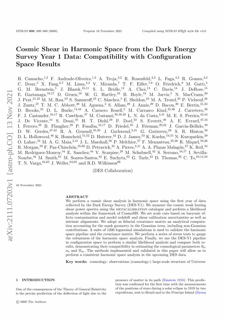
Figure 4. Marginalized posterior distributions for a subset of pa-

rameters for a noiseless data vector analyses in both configuration

space (CS) and harmonic space (HS), with and without scale cuts(SC) Dashed lines are the input parameters.

likelihood, L, defined as

−2 logL(Θ) = χ2 =∑ij

(Di −Di(Θ))TC−1ij (Dj −Dj(Θ)),

(20)where Di and Di(Θ) are the entries of the measured and the-oretical prediction for the data vector, constructed by stack-ing the power spectra bandpowers CEE(ab)(`) for differentcombinations of tomographic bins pairs, (a, b), Θ representsthe set of parameters, cosmological and nuisance, used inthe analysis, and C is the covariance matrix.

6.1 Validation with a noiseless data vector

We begin by validating this pipeline using a noiseless an-alytically computed data vector generated with the flaskcosmology. We used our pipeline for the likelihood analysesboth in configuration and harmonic space, with and with-out scale cuts motivated to mitigate baryonic effects and thesame binning as described in Section 5.2. For the configu-ration space run, we follow the DES-Y1 setup (Troxel et al.2018) again. Figure 4 shows the 2D posterior probabilitydistributions and constraints for a subset of the inferred pa-rameters, namely S8, Ωm and σ8. Figure 5 provides the 1Dmarginalized values of the parameters S8, Ωm, σ8, h0, Ωband ns. We conclude that the likelihood pipeline is work-ing as expected in this case, with consistent values for therecovered parameters and error bars.

MNRAS 000, 000–000 (0000)

8 DES Collaboration

0.75 0.80S8

CS, no SCs

CS, 2% baryonic-eff SCs

HS, no SCs

HS, 2% baryonic-eff SCs

0.25 0.30Ωm

0.7 0.8σ8

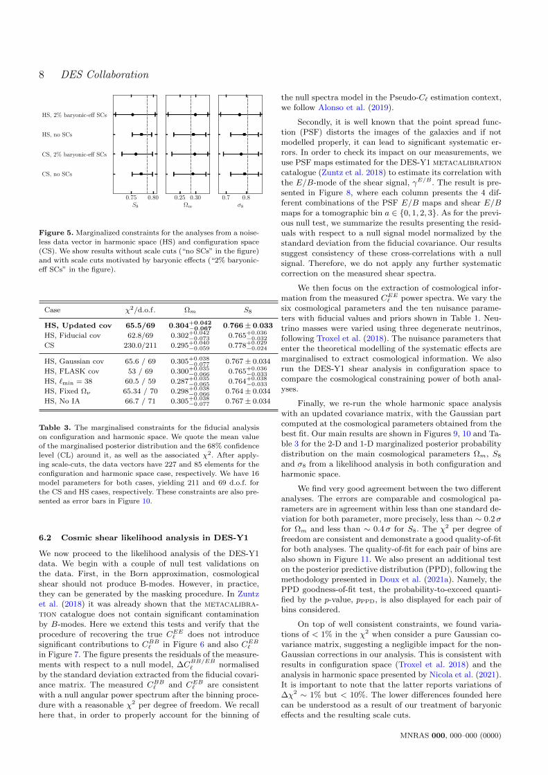
Figure 5. Marginalized constraints for the analyses from a noise-

less data vector in harmonic space (HS) and configuration space

(CS). We show results without scale cuts (“no SCs” in the figure)and with scale cuts motivated by baryonic effects (“2% baryonic-

eff SCs” in the figure).

Case χ2/d.o.f. Ωm S8

HS, Updated cov 65.5/69 0.304+0.042−0.067 0.766± 0.033

HS, Fiducial cov 62.8/69 0.302+0.042−0.073 0.765+0.036

−0.032

CS 230.0/211 0.295+0.040−0.059 0.778+0.029

−0.024

HS, Gaussian cov 65.6 / 69 0.305+0.038−0.077 0.767 ± 0.034

HS, FLASK cov 53 / 69 0.300+0.035−0.066 0.765+0.036

−0.033

HS, `min = 38 60.5 / 59 0.287+0.035−0.065 0.764+0.038

−0.033

HS, Fixed Ων 65.34 / 70 0.298+0.038−0.066 0.764 ± 0.034

HS, No IA 66.7 / 71 0.305+0.038−0.077 0.767 ± 0.034

Table 3. The marginalised constraints for the fiducial analysis

on configuration and harmonic space. We quote the mean value

of the marginalised posterior distribution and the 68% confidencelevel (CL) around it, as well as the associated χ2. After apply-

ing scale-cuts, the data vectors have 227 and 85 elements for theconfiguration and harmonic space case, respectively. We have 16

model parameters for both cases, yielding 211 and 69 d.o.f. for

the CS and HS cases, respectively. These constraints are also pre-sented as error bars in Figure 10.

6.2 Cosmic shear likelihood analysis in DES-Y1

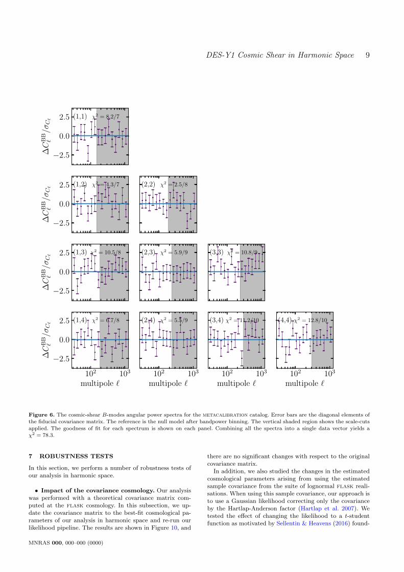
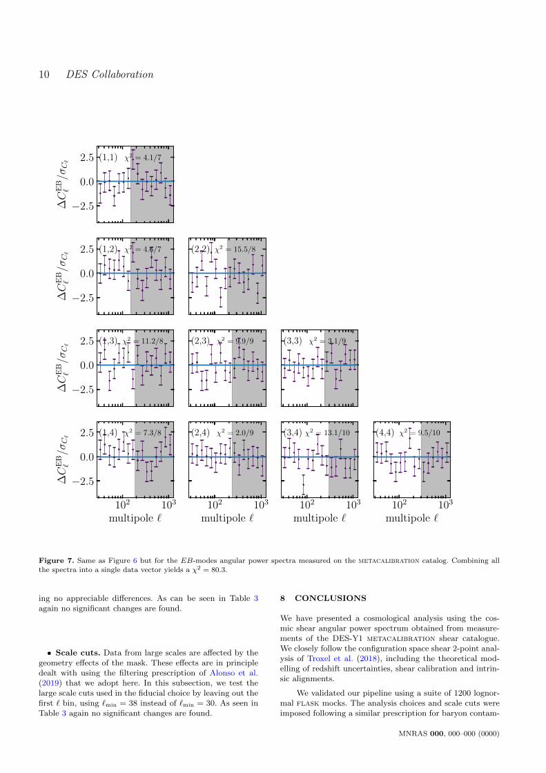
We now proceed to the likelihood analysis of the DES-Y1data. We begin with a couple of null test validations onthe data. First, in the Born approximation, cosmologicalshear should not produce B-modes. However, in practice,they can be generated by the masking procedure. In Zuntzet al. (2018) it was already shown that the metacalibra-tion catalogue does not contain significant contaminationby B-modes. Here we extend this tests and verify that theprocedure of recovering the true CEE` does not introducesignificant contributions to CBB` in Figure 6 and also CEB`in Figure 7. The figure presents the residuals of the measure-ments with respect to a null model, ∆C

BB/EB` normalised

by the standard deviation extracted from the fiducial covari-ance matrix. The measured CBB` and CEB` are consistentwith a null angular power spectrum after the binning proce-dure with a reasonable χ2 per degree of freedom. We recallhere that, in order to properly account for the binning of

the null spectra model in the Pseudo-C` estimation context,we follow Alonso et al. (2019).

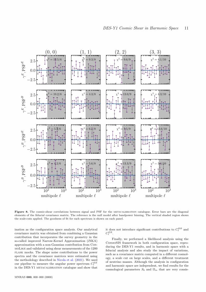
Secondly, it is well known that the point spread func-tion (PSF) distorts the images of the galaxies and if notmodelled properly, it can lead to significant systematic er-rors. In order to check its impact on our measurements, weuse PSF maps estimated for the DES-Y1 metacalibrationcatalogue (Zuntz et al. 2018) to estimate its correlation withthe E/B-mode of the shear signal, γE/B . The result is pre-sented in Figure 8, where each column presents the 4 dif-ferent combinations of the PSF E/B maps and shear E/Bmaps for a tomographic bin a ∈ 0, 1, 2, 3. As for the previ-ous null test, we summarize the results presenting the resid-uals with respect to a null signal model normalized by thestandard deviation from the fiducial covariance. Our resultssuggest consistency of these cross-correlations with a nullsignal. Therefore, we do not apply any further systematiccorrection on the measured shear spectra.

We then focus on the extraction of cosmological infor-mation from the measured CEE` power spectra. We vary thesix cosmological parameters and the ten nuisance parame-ters with fiducial values and priors shown in Table 1. Neu-trino masses were varied using three degenerate neutrinos,following Troxel et al. (2018). The nuisance parameters thatenter the theoretical modelling of the systematic effects aremarginalised to extract cosmological information. We alsorun the DES-Y1 shear analysis in configuration space tocompare the cosmological constraining power of both anal-yses.

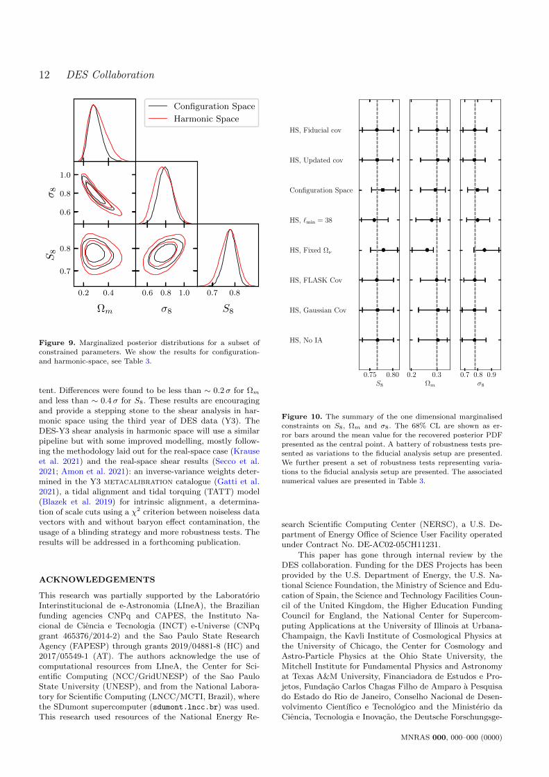
Finally, we re-run the whole harmonic space analysiswith an updated covariance matrix, with the Gaussian partcomputed at the cosmological parameters obtained from thebest fit. Our main results are shown in Figures 9, 10 and Ta-ble 3 for the 2-D and 1-D marginalized posterior probabilitydistribution on the main cosmological parameters Ωm, S8

and σ8 from a likelihood analysis in both configuration andharmonic space.

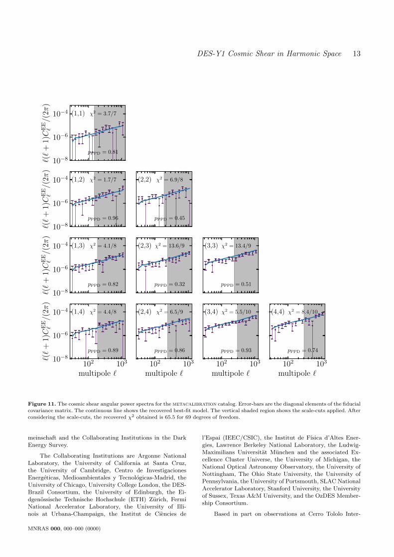
We find very good agreement between the two differentanalyses. The errors are comparable and cosmological pa-rameters are in agreement within less than one standard de-viation for both parameter, more precisely, less than ∼ 0.2σfor Ωm and less than ∼ 0.4σ for S8. The χ2 per degree offreedom are consistent and demonstrate a good quality-of-fitfor both analyses. The quality-of-fit for each pair of bins arealso shown in Figure 11. We also present an additional teston the posterior predictive distribution (PPD), following themethodology presented in Doux et al. (2021a). Namely, thePPD goodness-of-fit test, the probability-to-exceed quanti-fied by the p-value, pPPD, is also displayed for each pair ofbins considered.

On top of well consistent constraints, we found varia-tions of < 1% in the χ2 when consider a pure Gaussian co-variance matrix, suggesting a negligible impact for the non-Gaussian corrections in our analysis. This is consistent withresults in configuration space (Troxel et al. 2018) and theanalysis in harmonic space presented by Nicola et al. (2021).It is important to note that the latter reports variations of∆χ2 ∼ 1% but < 10%. The lower differences founded herecan be understood as a result of our treatment of baryoniceffects and the resulting scale cuts.

MNRAS 000, 000–000 (0000)

DES-Y1 Cosmic Shear in Harmonic Space 9

−2.5

0.0

2.5

∆C

BB

`/σ

C` (1,1) χ2 = 8.2/7

−2.5

0.0

2.5

∆C

BB

`/σ

C` (1,2) χ2 = 4.3/7 (2,2) χ2 = 2.5/8

−2.5

0.0

2.5

∆C

BB

`/σ

C` (1,3) χ2 = 10.5/8 (2,3) χ2 = 5.9/9 (3,3) χ2 = 10.8/9

102 103

multipole `

−2.5

0.0

2.5

∆C

BB

`/σ

C` (1,4) χ2 = 6.7/8

102 103

multipole `

(2,4) χ2 = 5.5/9

102 103

multipole `

(3,4) χ2 = 11.2/10

102 103

multipole `

(4,4) χ2 = 12.8/10

Figure 6. The cosmic-shear B-modes angular power spectra for the metacalibration catalog. Error bars are the diagonal elements of

the fiducial covariance matrix. The reference is the null model after bandpower binning. The vertical shaded region shows the scale-cutsapplied. The goodness of fit for each spectrum is shown on each panel. Combining all the spectra into a single data vector yields aχ2 = 78.3.

7 ROBUSTNESS TESTS

In this section, we perform a number of robustness tests ofour analysis in harmonic space.

• Impact of the covariance cosmology. Our analysiswas performed with a theoretical covariance matrix com-puted at the flask cosmology. In this subsection, we up-date the covariance matrix to the best-fit cosmological pa-rameters of our analysis in harmonic space and re-run ourlikelihood pipeline. The results are shown in Figure 10, and

there are no significant changes with respect to the originalcovariance matrix.

In addition, we also studied the changes in the estimatedcosmological parameters arising from using the estimatedsample covariance from the suite of lognormal flask reali-sations. When using this sample covariance, our approach isto use a Gaussian likelihood correcting only the covarianceby the Hartlap-Anderson factor (Hartlap et al. 2007). Wetested the effect of changing the likelihood to a t-studentfunction as motivated by Sellentin & Heavens (2016) found-

MNRAS 000, 000–000 (0000)

10 DES Collaboration

−2.5

0.0

2.5

∆C

EB

`/σ

C` (1,1) χ2 = 4.1/7

−2.5

0.0

2.5

∆C

EB

`/σ

C` (1,2) χ2 = 4.6/7 (2,2) χ2 = 15.5/8

−2.5

0.0

2.5

∆C

EB

`/σ

C` (1,3) χ2 = 11.2/8 (2,3) χ2 = 9.9/9 (3,3) χ2 = 3.1/9

102 103

multipole `

−2.5

0.0

2.5

∆C

EB

`/σ

C` (1,4) χ2 = 7.3/8

102 103

multipole `

(2,4) χ2 = 2.0/9

102 103

multipole `

(3,4) χ2 = 13.1/10

102 103

multipole `

(4,4) χ2 = 9.5/10

Figure 7. Same as Figure 6 but for the EB-modes angular power spectra measured on the metacalibration catalog. Combining all

the spectra into a single data vector yields a χ2 = 80.3.

ing no appreciable differences. As can be seen in Table 3again no significant changes are found.

• Scale cuts. Data from large scales are affected by thegeometry effects of the mask. These effects are in principledealt with using the filtering prescription of Alonso et al.(2019) that we adopt here. In this subsection, we test thelarge scale cuts used in the fiducial choice by leaving out thefirst ` bin, using `min = 38 instead of `min = 30. As seen inTable 3 again no significant changes are found.

8 CONCLUSIONS

We have presented a cosmological analysis using the cos-mic shear angular power spectrum obtained from measure-ments of the DES-Y1 metacalibration shear catalogue.We closely follow the configuration space shear 2-point anal-ysis of Troxel et al. (2018), including the theoretical mod-elling of redshift uncertainties, shear calibration and intrin-sic alignments.

We validated our pipeline using a suite of 1200 lognor-mal flask mocks. The analysis choices and scale cuts wereimposed following a similar prescription for baryon contam-

MNRAS 000, 000–000 (0000)

DES-Y1 Cosmic Shear in Harmonic Space 11

−2.5

0.0

2.5

γE,P

SFE

χ2 = 12.5/6

(0, 0)

χ2 = 9.3/8

(1, 1)

χ2 = 9.6/9

(2, 2)

χ2 = 4.1/10

(3, 3)

−2.5

0.0

2.5

γE,P

SFB

χ2 = 10.2/6 χ2 = 4.3/8 χ2 = 13.0/9 χ2 = 4.3/10

−2.5

0.0

2.5

γB,P

SFE

χ2 = 5.4/6 χ2 = 6.7/8 χ2 = 7.5/9 χ2 = 13.6/10

102 103

multipole `

−2.5

0.0

2.5

γB,P

SFB

χ2 = 4.2/6

102 103

multipole `

χ2 = 5.6/8

102 103

multipole `

χ2 = 13.3/9

102 103

multipole `

χ2 = 3.6/10

Figure 8. The cosmic-shear correlations between signal and PSF for the metacalibration catalogue. Error bars are the diagonal

elements of the fiducial covariance matrix. The reference is the null model after bandpower binning. The vertical shaded region showsthe scale-cuts applied. The goodness of fit for each spectrum is shown on each panel.

ination as the configuration space analysis. Our analyticalcovariance matrix was obtained from combining a Gaussiancontribution that incorporates the survey geometry in theso-called improved Narrow-Kernel Approximation (iNKA)approximation with a non-Gaussian contribution from Cos-moLike and validated using shear measurements of the 1200flask mocks. The shape noise contributions to the powerspectra and the covariance matrices were estimated usingthe methodology described in Nicola et al. (2021). We usedour pipeline to measure the angular power spectrum CEE`in the DES-Y1 metacalibration catalogue and show that

it does not introduce significant contributions to CBB` andCEB` .

Finally, we performed a likelihood analysis using theCosmoSIS framework in both configuration space, repro-ducing the DES-Y1 results, and in harmonic space with afiducial analysis and also study the impact of variations,such as a covariance matrix computed in a different cosmol-ogy, a scale cut on large scales, and a different treatmentof neutrino masses. Although the analysis in configurationand harmonic space are independent, we find results for thecosmological parameters S8 and Ωm that are very consis-

MNRAS 000, 000–000 (0000)

12 DES Collaboration

0.2 0.4

Ωm

0.7

0.8

S8

0.6

0.8

1.0

σ8

0.6 0.8 1.0

σ8

0.7 0.8

S8

Configuration Space

Harmonic Space

Figure 9. Marginalized posterior distributions for a subset of

constrained parameters. We show the results for configuration-and harmonic-space, see Table 3.

tent. Differences were found to be less than ∼ 0.2σ for Ωmand less than ∼ 0.4σ for S8. These results are encouragingand provide a stepping stone to the shear analysis in har-monic space using the third year of DES data (Y3). TheDES-Y3 shear analysis in harmonic space will use a similarpipeline but with some improved modelling, mostly follow-ing the methodology laid out for the real-space case (Krauseet al. 2021) and the real-space shear results (Secco et al.2021; Amon et al. 2021): an inverse-variance weights deter-mined in the Y3 metacalibration catalogue (Gatti et al.2021), a tidal alignment and tidal torquing (TATT) model(Blazek et al. 2019) for intrinsic alignment, a determina-tion of scale cuts using a χ2 criterion between noiseless datavectors with and without baryon effect contamination, theusage of a blinding strategy and more robustness tests. Theresults will be addressed in a forthcoming publication.

ACKNOWLEDGEMENTS

This research was partially supported by the LaboratorioInterinstitucional de e-Astronomia (LIneA), the Brazilianfunding agencies CNPq and CAPES, the Instituto Na-cional de Ciencia e Tecnologia (INCT) e-Universe (CNPqgrant 465376/2014-2) and the Sao Paulo State ResearchAgency (FAPESP) through grants 2019/04881-8 (HC) and2017/05549-1 (AT). The authors acknowledge the use ofcomputational resources from LIneA, the Center for Sci-entific Computing (NCC/GridUNESP) of the Sao PauloState University (UNESP), and from the National Labora-tory for Scientific Computing (LNCC/MCTI, Brazil), wherethe SDumont supercomputer (sdumont.lncc.br) was used.This research used resources of the National Energy Re-

0.75 0.80S8

HS, No IA

HS, Gaussian Cov

HS, FLASK Cov

HS, Fixed Ων

HS, `min = 38

Configuration Space

HS, Updated cov

HS, Fiducial cov

0.2 0.3Ωm

0.7 0.8 0.9σ8

Figure 10. The summary of the one dimensional marginalised

constraints on S8, Ωm and σ8. The 68% CL are shown as er-

ror bars around the mean value for the recovered posterior PDFpresented as the central point. A battery of robustness tests pre-

sented as variations to the fiducial analysis setup are presented.

We further present a set of robustness tests representing varia-tions to the fiducial analysis setup are presented. The associated

numerical values are presented in Table 3.

search Scientific Computing Center (NERSC), a U.S. De-partment of Energy Office of Science User Facility operatedunder Contract No. DE-AC02-05CH11231.

This paper has gone through internal review by theDES collaboration. Funding for the DES Projects has beenprovided by the U.S. Department of Energy, the U.S. Na-tional Science Foundation, the Ministry of Science and Edu-cation of Spain, the Science and Technology Facilities Coun-cil of the United Kingdom, the Higher Education FundingCouncil for England, the National Center for Supercom-puting Applications at the University of Illinois at Urbana-Champaign, the Kavli Institute of Cosmological Physics atthe University of Chicago, the Center for Cosmology andAstro-Particle Physics at the Ohio State University, theMitchell Institute for Fundamental Physics and Astronomyat Texas A&M University, Financiadora de Estudos e Pro-jetos, Fundacao Carlos Chagas Filho de Amparo a Pesquisado Estado do Rio de Janeiro, Conselho Nacional de Desen-volvimento Cientıfico e Tecnologico and the Ministerio daCiencia, Tecnologia e Inovacao, the Deutsche Forschungsge-

MNRAS 000, 000–000 (0000)

DES-Y1 Cosmic Shear in Harmonic Space 13

10−8

10−6

10−4

`(`

+1)C

EE

`/(

2π)

(1,1) χ2 = 3.7/7

pPPD = 0.81

10−8

10−6

10−4

`(`

+1)C

EE

`/(

2π)

(1,2) χ2 = 1.7/7

pPPD = 0.96

(2,2) χ2 = 6.9/8

pPPD = 0.45

10−8

10−6

10−4

`(`

+1)C

EE

`/(

2π)

(1,3) χ2 = 4.1/8

pPPD = 0.82

(2,3) χ2 = 13.6/9

pPPD = 0.32

(3,3) χ2 = 13.4/9

pPPD = 0.51

102 103

multipole `

10−8

10−6

10−4

`(`

+1)C

EE

`/(

2π)

(1,4) χ2 = 4.4/8

pPPD = 0.89

102 103

multipole `

(2,4) χ2 = 6.5/9

pPPD = 0.86

102 103

multipole `

(3,4) χ2 = 5.5/10

pPPD = 0.93

102 103

multipole `

(4,4) χ2 = 8.4/10

pPPD = 0.74

Figure 11. The cosmic shear angular power spectra for the metacalibration catalog. Error-bars are the diagonal elements of the fiducial

covariance matrix. The continuous line shows the recovered best-fit model. The vertical shaded region shows the scale-cuts applied. Afterconsidering the scale-cuts, the recovered χ2 obtained is 65.5 for 69 degrees of freedom.

meinschaft and the Collaborating Institutions in the DarkEnergy Survey.

The Collaborating Institutions are Argonne NationalLaboratory, the University of California at Santa Cruz,the University of Cambridge, Centro de InvestigacionesEnergeticas, Medioambientales y Tecnologicas-Madrid, theUniversity of Chicago, University College London, the DES-Brazil Consortium, the University of Edinburgh, the Ei-dgenossische Technische Hochschule (ETH) Zurich, FermiNational Accelerator Laboratory, the University of Illi-nois at Urbana-Champaign, the Institut de Ciencies de

l’Espai (IEEC/CSIC), the Institut de Fısica d’Altes Ener-gies, Lawrence Berkeley National Laboratory, the Ludwig-Maximilians Universitat Munchen and the associated Ex-cellence Cluster Universe, the University of Michigan, theNational Optical Astronomy Observatory, the University ofNottingham, The Ohio State University, the University ofPennsylvania, the University of Portsmouth, SLAC NationalAccelerator Laboratory, Stanford University, the Universityof Sussex, Texas A&M University, and the OzDES Member-ship Consortium.

Based in part on observations at Cerro Tololo Inter-

MNRAS 000, 000–000 (0000)

14 DES Collaboration

American Observatory at NSF’s NOIRLab (NOIRLab Prop.ID 2012B-0001; PI: J. Frieman), which is managed bythe Association of Universities for Research in Astronomy(AURA) under a cooperative agreement with the NationalScience Foundation.

The DES data management system is supported bythe National Science Foundation under Grant NumbersAST-1138766 and AST-1536171. The DES participants fromSpanish institutions are partially supported by MINECOunder grants AYA2015-71825, ESP2015-66861, FPA2015-68048, SEV-2016-0588, SEV-2016-0597, and MDM-2015-0509, some of which include ERDF funds from the EuropeanUnion. IFAE is partially funded by the CERCA programof the Generalitat de Catalunya. Research leading to theseresults has received funding from the European ResearchCouncil under the European Union’s Seventh FrameworkProgram (FP7/2007-2013) including ERC grant agreements240672, 291329, and 306478.

This manuscript has been authored by Fermi ResearchAlliance, LLC under Contract No. DE-AC02-07CH11359with the U.S. Department of Energy, Office of Science, Officeof High Energy Physics.

This work made use of the software packagesmatplotlib (Hunter 2007), and numpy (Harris et al. 2020).

DATA AVAILABILITY STATEMENT

The DES Y1 catalog is available in the Dark En-ergy Survey Data Management (DESDM) system atthe National Center for Supercomputing Applications(NCSA) at the University of Illinois. It can beaccessed at https://des.ncsa.illinois.edu/releases/

y1a1/key-catalogs. The pipeline used for the measurementis publicly available at https://github.com/hocamachoc/

3x2hs_measurements. Synthetic data produced by the anal-ysis presented here can be shared on request to the corre-sponding author.

REFERENCES

Alonso D., Sanchez J., Slosar A., LSST Dark Energy Science Col-

laboration 2019, MNRAS, 484, 4127

Amon A., et al., 2021, arXiv e-prints, p. arXiv:2105.13543

Andrade-Oliveira F., et al., 2021, MNRAS, 505, 5714

Asgari M., et al., 2021, A&A, 645, A104

Bartelmann M., Schneider P., 2001, Phys. Rep., 340, 291

Benıtez N., 2000, ApJ, 536, 571

Blazek J. A., MacCrann N., Troxel M. A., Fang X., 2019, Phys.

Rev. D, 100, 103506

Bridle S., King L., 2007, New Journal of Physics, 9, 444

Chang C., et al., 2018, MNRAS, 475, 3165

Chang C., et al., 2019, MNRAS, 482, 3696

DES Collaboration et al., 2021, arXiv e-prints, p.

arXiv:2107.04646

Davis C., et al., 2017, arXiv e-prints, p. arXiv:1710.02517

Dodelson S., 2017, Gravitational Lensing. Cambridge UniversityPress

Doux C., et al., 2021a, MNRAS, 503, 2688

Doux C., et al., 2021b, MNRAS, 503, 3796

Dyson F. W., Eddington A. S., Davidson C., 1920, Philosophical

Transactions of the Royal Society of London Series A, 220,

291

Einstein A., 1916, Annalen Phys., 49, 769

Feroz F., Hobson M. P., Bridges M., 2009, MNRAS, 398, 1601

Friedrich O., et al., 2018, Phys. Rev. D, 98, 023508

Friedrich O., et al., 2021, MNRAS,

Garcıa-Garcıa C., Alonso D., Bellini E., 2019, J. Cosmology As-

tropart. Phys., 2019, 043

Gatti M., et al., 2018, MNRAS, 477, 1664

Gatti M., et al., 2021, MNRAS, 504, 4312

Gorski K. M., Hivon E., Banday A. J., Wandelt B. D., Hansen

F. K., Reinecke M., Bartelmann M., 2005, ApJ, 622, 759

Hadzhiyska B., Garcıa-Garcıa C., Alonso D., Nicola A., Slosar A.,

2021, J. Cosmology Astropart. Phys., 2021, 020

Hamana T., et al., 2020, PASJ, 72, 16

Harris C. R., et al., 2020, Nature, 585, 357

Hartlap J., Simon P., Schneider P., 2007, A&A, 464, 399

Heymans C., et al., 2006, MNRAS, 368, 1323

Hikage C., et al., 2019, PASJ, 71, 43

Hildebrandt H., et al., 2017, MNRAS, 465, 1454

Hivon E., Gorski K. M., Netterfield C. B., Crill B. P., Prunet S.,Hansen F., 2002, ApJ, 567, 2

Howlett C., Lewis A., Hall A., Challinor A., 2012, J. CosmologyAstropart. Phys., 2012, 027

Hoyle B., et al., 2018, MNRAS, 478, 592

Huang H.-J., et al., 2021, MNRAS, 502, 6010

Huff E., Mandelbaum R., 2017, arXiv e-prints, p.

arXiv:1702.02600

Hunter J. D., 2007, Computing in Science and Engineering, 9, 90

Huterer D., Takada M., Bernstein G., Jain B., 2006, MNRAS,366, 101

Jee M. J., Tyson J. A., Schneider M. D., Wittman D., SchmidtS., Hilbert S., 2013, ApJ, 765, 74

Jee M. J., Tyson J. A., Hilbert S., Schneider M. D., Schmidt S.,Wittman D., 2016, ApJ, 824, 77

Joudaki S., et al., 2017, MNRAS, 465, 2033

Joudaki S., et al., 2020, A&A, 638, L1

Kirk D., Rassat A., Host O., Bridle S., 2012, MNRAS, 424, 1647

Kitching T. D., Alsing J., Heavens A. F., Jimenez R., McEwen

J. D., Verde L., 2017, MNRAS, 469, 2737

Krause E., Eifler T., 2017, MNRAS, 470, 2100

Krause E., et al., 2017, arXiv e-prints, p. arXiv:1706.09359

Krause E., et al., 2021, arXiv e-prints, p. arXiv:2105.13548

Lewis A., Challinor A., Lasenby A., 2000, ApJ, 538, 473

Limber D. N., 1953, ApJ, 117, 134

LoVerde M., Afshordi N., 2008, Phys. Rev. D, 78, 123506

Mandelbaum R., 2018, ARA&A, 56, 393

Moreira M. G., Andrade-Oliveira F., Fang X., Huang H.-J.,Krause E., Miranda V., Rosenfeld R., Simonovic M., 2021,

MNRAS, 507, 5592

Nicola A., Garcıa-Garcıa C., Alonso D., Dunkley J., Ferreira

P. G., Slosar A., Spergel D. N., 2021, J. Cosmology Astropart.Phys., 2021, 067

Schaye J., et al., 2010, MNRAS, 402, 1536

Secco L. F., et al., 2021, arXiv e-prints, p. arXiv:2105.13544

Sellentin E., Heavens A. F., 2016, MNRAS, 456, L132

Sheldon E. S., Huff E. M., 2017, ApJ, 841, 24

Smith R. E., et al., 2003, MNRAS, 341, 1311

Takahashi R., Sato M., Nishimichi T., Taruya A., Oguri M., 2012,

ApJ, 761, 152

Taylor A., Joachimi B., Kitching T., 2013, MNRAS, 432, 1928

Troxel M. A., et al., 2018, Phys. Rev. D, 98, 043528

Xavier H. S., Abdalla F. B., Joachimi B., 2016, MNRAS, 459,3693

Zuntz J., et al., 2015, Astronomy and Computing, 12, 45

Zuntz J., et al., 2018, MNRAS, 481, 1149

van Daalen M. P., Schaye J., Booth C. M., Dalla Vecchia C., 2011,MNRAS, 415, 3649

MNRAS 000, 000–000 (0000)

DES-Y1 Cosmic Shear in Harmonic Space 15

AUTHOR AFFILIATIONS

1 Instituto de Fısica Teorica, Universidade EstadualPaulista, Sao Paulo, Brazil2 Laboratorio Interinstitucional de e-Astronomia - LIneA,Rua Gal. Jose Cristino 77, Rio de Janeiro, RJ - 20921-400,Brazil3 ICTP South American Institute for Fundamental Re-searchInstituto de Fısica Teorica, Universidade Estadual Paulista,Sao Paulo, Brazil4 Departamento de Fısica Matematica, Instituto de Fısica,Universidade de Sao Paulo, CP 66318, Sao Paulo, SP,05314-970, Brazil5 Department of Physics and Astronomy, University ofPennsylvania, Philadelphia, PA 19104, USA6 Department of Astronomy, University of California,Berkeley, 501 Campbell Hall, Berkeley, CA 94720, USA7 Department of Astronomy/Steward Observatory, Uni-versity of Arizona, 933 North Cherry Avenue, Tucson, AZ85721-0065, USA8 Jet Propulsion Laboratory, California Institute of Tech-nology, 4800 Oak Grove Dr., Pasadena, CA 91109, USA9 Kavli Institute for Cosmology, University of Cambridge,Madingley Road, Cambridge CB3 0HA, UK10 Department of Physics, Northeastern University, Boston,MA 02115, USA11 Laboratory of Astrophysics, Ecole PolytechniqueFederale de Lausanne (EPFL), Observatoire de Sauverny,1290 Versoix, Switzerland12 Jodrell Bank Center for Astrophysics, School of Physicsand Astronomy, University of Manchester, Oxford Road,Manchester, M13 9PL, UK13 California Institute of Technology, 1200 East CaliforniaBlvd, MC 249-17, Pasadena, CA 91125, USA14 Kavli Institute for Particle Astrophysics & Cosmology,P. O. Box 2450, Stanford University, Stanford, CA 94305,USA15 Lawrence Berkeley National Laboratory, 1 CyclotronRoad, Berkeley, CA 94720, USA16 Institut d’Estudis Espacials de Catalunya (IEEC), 08034Barcelona, Spain17 Institute of Space Sciences (ICE, CSIC), Campus UAB,Carrer de Can Magrans, s/n, 08193 Barcelona, Spain18 Faculty of Physics, Ludwig-Maximilians-Universitat,Scheinerstr. 1, 81679 Munich, Germany19 Department of Astronomy, University of Geneva, ch.d’Ecogia 16, CH-1290 Versoix, Switzerland20 Department of Applied Mathematics and TheoreticalPhysics, University of Cambridge, Cambridge CB3 0WA,UK21 Department of Astronomy and Astrophysics, Universityof Chicago, Chicago, IL 60637, USA22 Kavli Institute for Cosmological Physics, University ofChicago, Chicago, IL 60637, USA23 Department of Physics, Carnegie Mellon University,Pittsburgh, Pennsylvania 15312, USA24 Brookhaven National Laboratory, Bldg 510, Upton, NY11973, USA25 Department of Physics, Duke University Durham, NC27708, USA26 Institut de Fısica d’Altes Energies (IFAE), The Barcelona

Institute of Science and Technology, Campus UAB, 08193Bellaterra (Barcelona) Spain27 Institute for Astronomy, University of Edinburgh, Edin-burgh EH9 3HJ, UK28 Cerro Tololo Inter-American Observatory, NSF’s Na-tional Optical-Infrared Astronomy Research Laboratory,Casilla 603, La Serena, Chile29 Fermi National Accelerator Laboratory, P. O. Box 500,Batavia, IL 60510, USA30 Institute of Cosmology and Gravitation, University ofPortsmouth, Portsmouth, PO1 3FX, UK31 CNRS, UMR 7095, Institut d’Astrophysique de Paris,F-75014, Paris, France32 Sorbonne Universites, UPMC Univ Paris 06, UMR 7095,Institut d’Astrophysique de Paris, F-75014, Paris, France33 Department of Physics & Astronomy, University CollegeLondon, Gower Street, London, WC1E 6BT, UK34 SLAC National Accelerator Laboratory, Menlo Park, CA94025, USA35 Center for Astrophysical Surveys, National Centerfor Supercomputing Applications, 1205 West Clark St.,Urbana, IL 61801, USA36 Department of Astronomy, University of Illinois atUrbana-Champaign, 1002 W. Green Street, Urbana, IL61801, USA37

38 Astronomy Unit, Department of Physics, University ofTrieste, via Tiepolo 11, I-34131 Trieste, Italy39 INAF-Osservatorio Astronomico di Trieste, via G. B.Tiepolo 11, I-34143 Trieste, Italy40 Institute for Fundamental Physics of the Universe, ViaBeirut 2, 34014 Trieste, Italy41 Observatorio Nacional, Rua Gal. Jose Cristino 77, Riode Janeiro, RJ - 20921-400, Brazil42 Department of Physics, University of Michigan, AnnArbor, MI 48109, USA43 Hamburger Sternwarte, Universitat Hamburg, Gojen-bergsweg 112, 21029 Hamburg, Germany44 Centro de Investigaciones Energeticas, Medioambientalesy Tecnologicas (CIEMAT), Madrid, Spain45 Department of Physics, IIT Hyderabad, Kandi, Telan-gana 502285, India46 Santa Cruz Institute for Particle Physics, Santa Cruz,CA 95064, USA47 Department of Astronomy, University of Michigan, AnnArbor, MI 48109, USA48 Institute of Theoretical Astrophysics, University of Oslo.P.O. Box 1029 Blindern, NO-0315 Oslo, Norway49 Instituto de Fisica Teorica UAM/CSIC, UniversidadAutonoma de Madrid, 28049 Madrid, Spain50 School of Mathematics and Physics, University ofQueensland, Brisbane, QLD 4072, Australia51 Center for Cosmology and Astro-Particle Physics, TheOhio State University, Columbus, OH 43210, USA52 Department of Physics, The Ohio State University,Columbus, OH 43210, USA53 Center for Astrophysics | Harvard & Smithsonian, 60Garden Street, Cambridge, MA 02138, USA54 Australian Astronomical Optics, Macquarie University,North Ryde, NSW 2113, Australia55 Lowell Observatory, 1400 Mars Hill Rd, Flagstaff, AZ86001, USA

MNRAS 000, 000–000 (0000)

16 DES Collaboration

56 George P. and Cynthia Woods Mitchell Institute forFundamental Physics and Astronomy, and Department ofPhysics and Astronomy, Texas A&M University, CollegeStation, TX 77843, USA57 Department of Astrophysical Sciences, Princeton Uni-versity, Peyton Hall, Princeton, NJ 08544, USA58 Institucio Catalana de Recerca i Estudis Avancats,E-08010 Barcelona, Spain59 Physics Department, 2320 Chamberlin Hall, Universityof Wisconsin-Madison, 1150 University Avenue Madison,WI 53706-139060 Institute of Astronomy, University of Cambridge, Mad-ingley Road, Cambridge CB3 0HA, UK61 School of Physics and Astronomy, University ofSouthampton, Southampton, SO17 1BJ, UK62 Computer Science and Mathematics Division, Oak RidgeNational Laboratory, Oak Ridge, TN 3783163 Department of Physics, Stanford University, 382 ViaPueblo Mall, Stanford, CA 94305, USA64 Max Planck Institute for Extraterrestrial Physics,Giessenbachstrasse, 85748 Garching, Germany65 Universitats-Sternwarte, Fakultat fur Physik, Ludwig-Maximilians Universitat Munchen, Scheinerstr. 1, 81679Munchen, Germany66 Department of Physics and Astronomy, Pevensey Build-ing, University of Sussex, Brighton, BN1 9QH, UK

MNRAS 000, 000–000 (0000)