Embed Size (px)
Citation preview

Cosinor analysis of accident risk using SPSS’s regression
procedures
Peter Watson
31st October 1997
MRC Cognition & Brain Sciences Unit

Aims & Objectives
• To help understand accident risk we investigate 3 alertness measures over time
– Two self-reported measures of sleep: Stanford Sleepiness Score (SSS) and Visual Analogue Score (VAS)
– Attention measure: Sustained Attention to Response Task (SART)

Study
• 10 healthy Peterhouse college undergrads
(5 male)
• Studied at 1am, 7am, 1pm and 7pm for four consecutive days
• How do vigilance (SART) and perceived vigilance (SSS, VAS) behave over time?
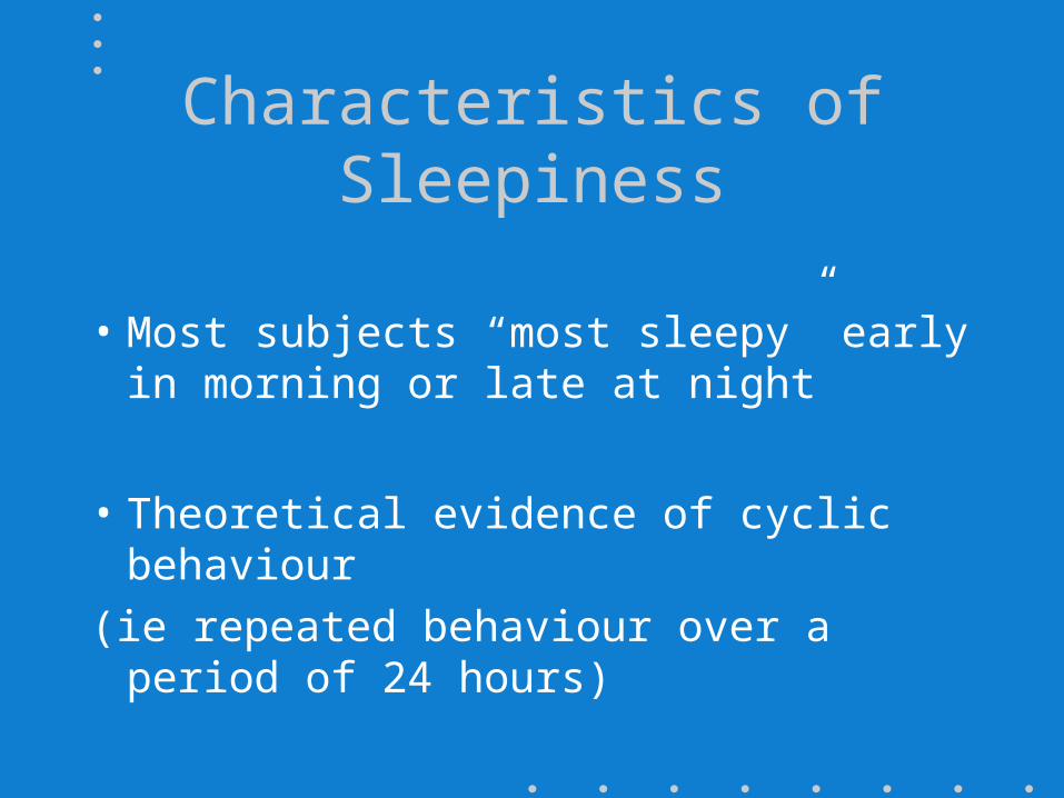
Characteristics of Sleepiness
• Most subjects “most sleepy” early in morning or late at night
• Theoretical evidence of cyclic behaviour
(ie repeated behaviour over a period of 24 hours)
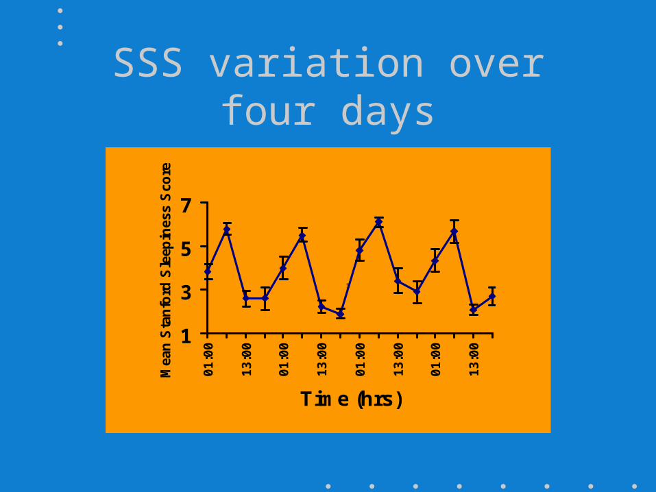
SSS variation over four days
1
3
5
70
1:0
0
13
:00
01
:00
13
:00
01
:00
13
:00
01
:00
13
:00
Time (hrs)
Mea
n S
tan
ford
Sle
epin
ess
Sco
re
1

VAS variation over four days
0
2
4
6
8
100
1:0
0
13
:00
01
:00
13
:00
01
:00
13
:00
01
:00
13
:00
Time (hrs)
Me
an
Vis
ua
l An
alo
gu
e S
lee
pin
ess
Sco
re

Aspects of cyclic behaviour
• Features considered:
• Length of a cycle (period)
• Overall value of response (mesor)
• Location of peak and nadir (acrophase)
• Half the difference between peak and nadir scores (amplitude)

Cosinor Model - cyclic behaviour
• f(t) = M + AMP.Cos(2t + ) + t
T
Parameters of Interest:
f(t) = sleepiness score;
M = intercept (Mesor);
AMP = amplitude; =phase; T=trial period (in hours) under study = 24; t = Residual

Period, T
• May be estimated
• Previous experience (as in our example)
• Constrained so that Peak and Nadir are T/2
hours apart (12 hours in our sleep example)

Periodicity
• 24 hour Periodicity upheld via absence of Time by Day interactions
• SSS : F(9,81)=0.57, p>0.8
• VAS : F(9,81)=0.63, p>0.7

Fitting using SPSS “linear” regression
For g(t)=2t/24 and since
Cos(g(t)+) = Cos()Cos(g(t))-Sin()Sin(g(t))
it follows the linear regression:
f(t) = M + A.Cos(2t/24) + B.Sin(2t/24)
is equivalent to the above single cosine function - now fittable in SPSS “linear” regression combining Cos and Sine function
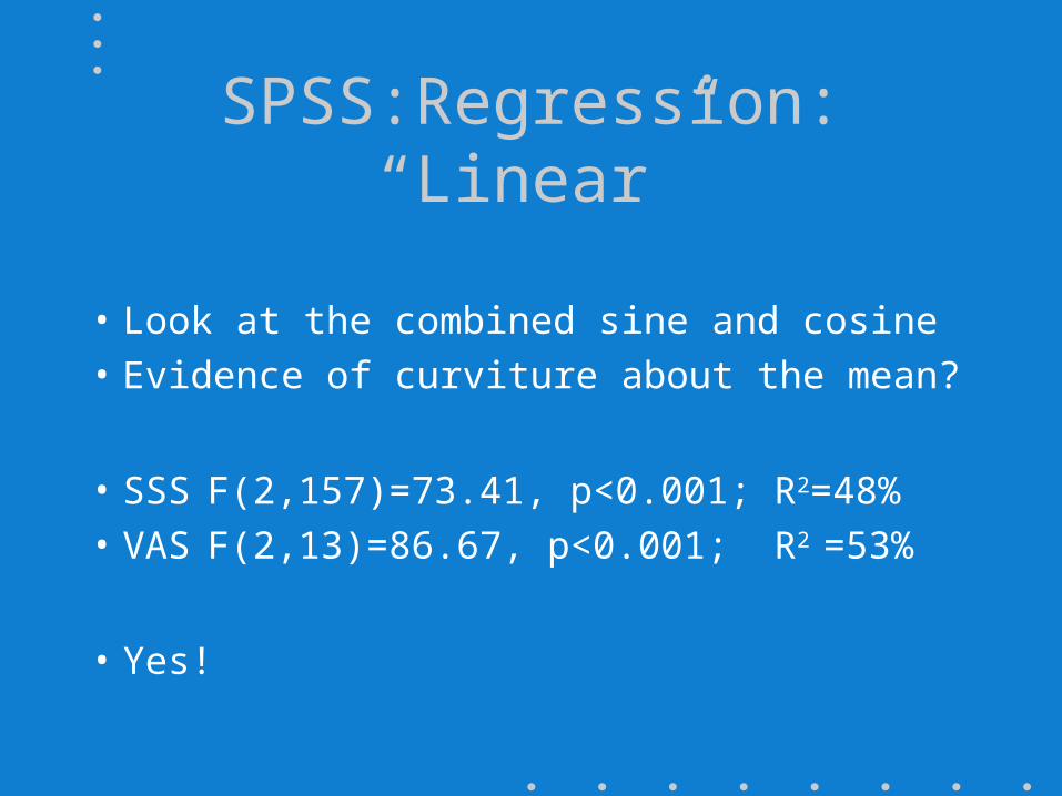
SPSS:Regression: “Linear”
• Look at the combined sine and cosine• Evidence of curviture about the mean?
• SSS F(2,157)=73.41, p<0.001; R2=48%• VAS F(2,13)=86.67, p<0.001; R2 =53%
• Yes!
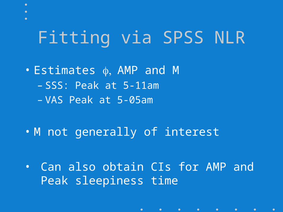
Fitting via SPSS NLR
• Estimates AMP and M– SSS: Peak at 5-11am– VAS Peak at 5-05am
• M not generally of interest
• Can also obtain CIs for AMP and Peak sleepiness time

Equivalence of NLR and “Linear” regression models
• Amplitude:
A = AMP Cos()
B = -AMP Sin()
Hence
AMP =
• Acrophase:
A = AMP Cos()
B = -AMP Sin()
Hence
ArcTan(-B/A)22 BA
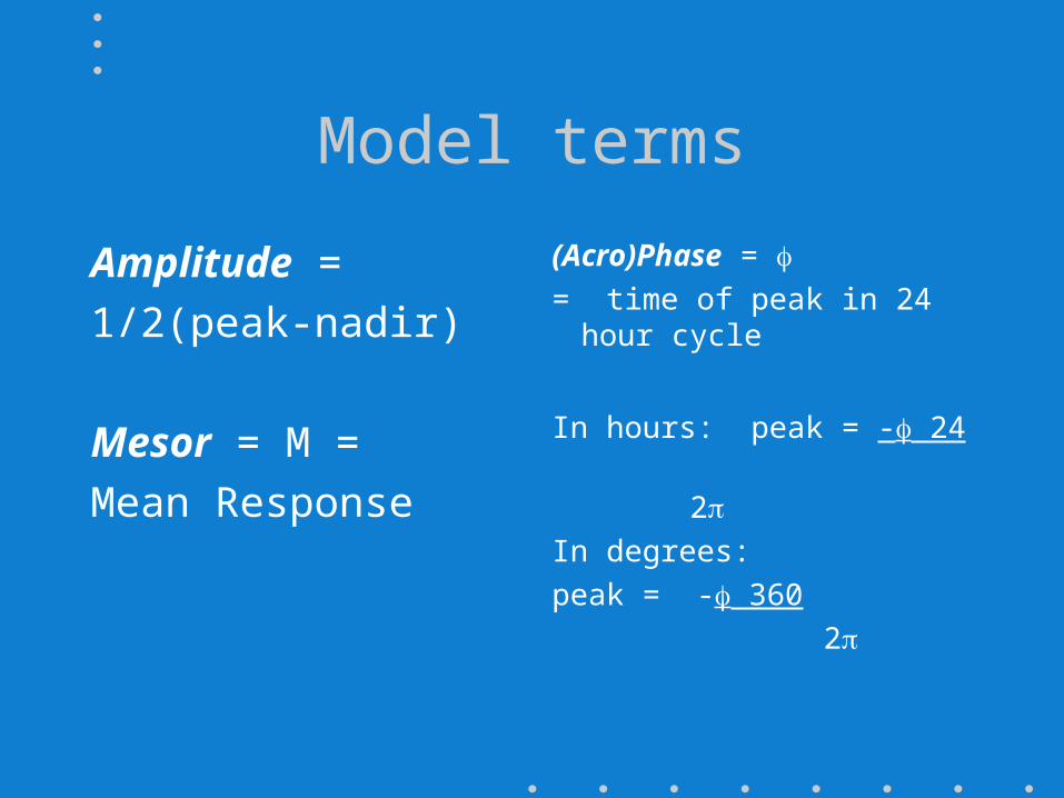
Model terms
Amplitude =
1/2(peak-nadir)
Mesor = M =
Mean Response
(Acro)Phase = = time of peak in 24 hour
cycle
In hours: peak = - 24
2
In degrees:
peak = - 360
2

Fitted Cosinor Functions (VAS in black; SSS in red)
0
1
2
3
4
5
6
7
8
9
1:00AM
7:00AM
1:00PM
7:00PM
1:00AM
Time of Day
Sle
ep
ine
ss
Sc
ore

% Amplitude
• % Amplitude = 100 x (Peak-Nadir)
overall mean
= 100 x 2 AMP
MESOR

95% Confidence interval for peak
• Use SPSS NLR - estimates acrophase directly
• acrophase ± t13,0.025 x standard error
• multiply endpoints by -3.82 (=-24/2)
• Ie
standard error(C.) = |Cx standard error()
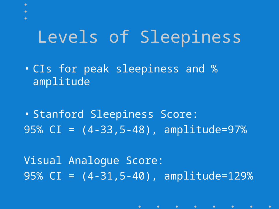
Levels of Sleepiness
• CIs for peak sleepiness and % amplitude
• Stanford Sleepiness Score:
95% CI = (4-33,5-48), amplitude=97%
Visual Analogue Score:
95% CI = (4-31,5-40), amplitude=129%
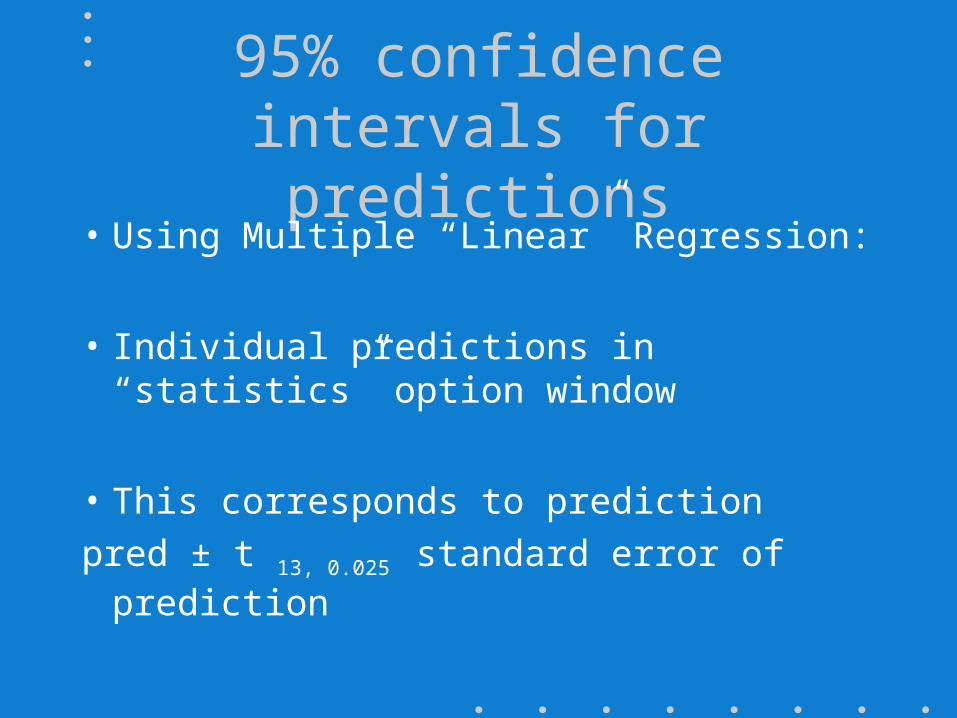
95% confidence intervals for predictions
• Using Multiple “Linear” Regression:
• Individual predictions in “statistics” option window
• This corresponds to prediction
pred ± t 13, 0.025 standard error of prediction

SSS - 95% Confidence Intervals
0
1
2
3
4
5
6
7
8
9
D A Y 1 D A Y 2 D A Y 3 D A Y 4
lowerupperpredictedmean

VAS 95% Confidence Intervals
0
2
4
6
8
10
12
14
D A Y 1 D A Y 2 D A Y 3 D A Y 4
MeanLowerUpperPredicted

Rules of Thumb for Fit
• De Prins J, Waldura J (1993)
• Acceptable Fit
95% CI phase range < 30 degrees
SSS 19 degrees (from NLR)
VAS 17 degrees (from NLR)

Conclusions
• Perceived alertness has a 24 hour cycle
• No Time by Day interaction - alertness consistent each day
• We feel most sleepy around early morning

Unperceived Vigilance
• Vigilance task (same 10 students as sleep indices)
• Proportion of correct responses to an attention task at 1am, 7am, 1pm and 7pm over 4 days
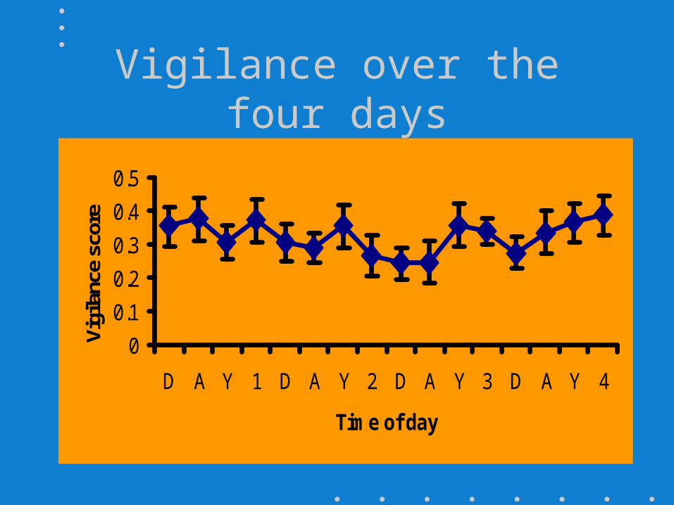
Vigilance over the four days
0
0.1
0.2
0.3
0.4
0.5
D A Y 1 D A Y 2 D A Y 3 D A Y 4
Time of day
Vigi
lanc
e sc
ore
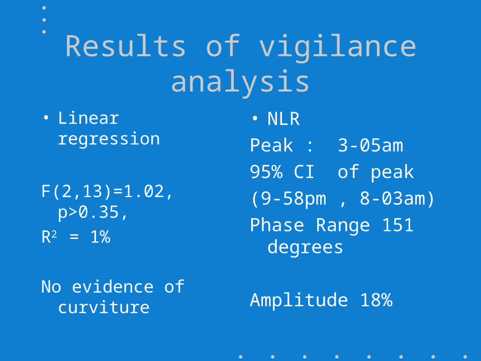
Results of vigilance analysis
• Linear regression
F(2,13)=1.02, p>0.35,
R2 = 1%
No evidence of curviture
• NLR
Peak : 3-05am
95% CI of peak
(9-58pm , 8-03am)
Phase Range 151 degrees
Amplitude 18%

Vigilance - linear over time
• Plot suggests no obvious periodicity
• Acrophase of 151 degrees > 30 degrees (badly inaccurate fit)
• Cyclic terms statistically nonsignificant, low R2
• Flat profile suggested by low % amplitude
• Vigilance, itself, may be linear with time

Polynomial Regression
• An alternative strategy is the fitting of cubic polynomials
• Similar results to cosinor functions – two turning points for perceived sleepiness– no turning points (linear) for attention measure
Conclusions
• Cosinor analysis is a natural way of modelling cyclic behaviour
• Can be fitted in SPSS using either “linear” or nonlinear regression procedures

Thanks to helpful colleagues…..
• Avijit Datta
• Geraint Lewis
• Tom Manly
• Ian Robertson


![C-MRC it gb de Ed01 2007reducta-im.hr/katalozi/zupcasti_reduktori_rc.pdfSELEZIONE RIDUTTORE - MRC 1400 [min-1] SPEED REDUCER SELECTION - MRC GETRIEBEAUSWAHL - MRC 0.09 kW (0.12 HP)](https://img.pdfslide.us/doc/110x75/6108c986e8f90f642023ce89/c-mrc-it-gb-de-ed01-2007reducta-imhrkatalozizupcastireduktorircpdf-selezione.jpg)